Author response:
The following is the authors’ response to the previous reviews
Responses to Editors:
We appreciate the editors’ concern regarding the difficulty of disentangling the contributions of tightly-coupled brain regions to the speech-gesture integration process—particularly due to the close temporal and spatial proximity of the stimulation windows and the potential for prolonged disruption. While we agree with that stimulation techniques, such as transcranial magnetic stimulation (TMS), can evoke or modulate neuronal activity both locally within the target region and in remote connected areas of the network. This complex interaction makes drawing clear conclusions about the causal relationship between stimulation and cognitive function more challenging. However, we believe that cause-and-effect relationships in cognitive neuroscience studies using non-invasive brain stimulation (NIBS) can still be robustly established if key assumptions are explicitly tested and confounding factors are rigorously controlled (Bergmann & Hartwigsen et al., 2021, J Cogn Neurosci).
In our experiment, we addressed these concerns by including a sham TMS condition, an irrelevant control task, and multiple control time points. The results showed that TMS selectively disrupted the IFG-pMTG interaction during specific time windows of the task related to gesture-speech semantic congruency, but not in the sham TMS condition or the control task (gender congruency effect) (Zhao et al., 2021, JN). This selective disruption provides strong evidence for a causal link between IFG-pMTG connectivity and gesture-speech integration in the targeted time window.
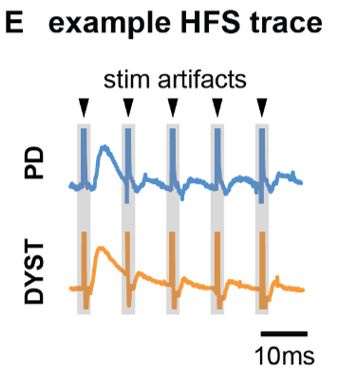
Regarding the potential for transient artifacts from TMS, we acknowledge that previous research has demonstrated that single-pulse TMS induces brief artifacts (0–10 ms) due to direct depolarization of cortical neurons, which momentarily disrupts electrical activity in the stimulated area (Romero et al., 2019, NC). However, in the case of paired-pulse TMS (ppTMS), the interaction between the first and second pulses is more complex. The first pulse increases membrane conductance in the target neurons via shunting inhibition mediated by GABAergic interneurons. This effectively lowers neuronal membrane resistance, “leaking” excitatory current and diminishing the depolarization induced by the second pulse, leading to a reduction in excitability during the paired-pulse interval. This mechanism suppresses the excitatory response to the second pulse, which is reflected in a reduced motor evoked potential (MEP) (Paulus & Rothwell, 2016, J Physiol).
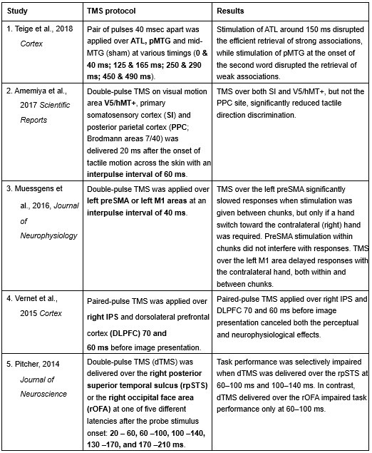
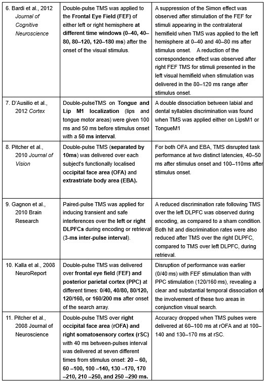
Furthermore, ppTMS has been widely used in previous studies to infer causal temporal relationships and explore the neural contributions of both structurally and functionally connected brain regions, across timescales as brief as 3–60 ms. We have reviewed several studies that employed paired-pulse TMS to investigate neural dynamics in regions such as the tongue and lip areas of the primary motor cortex (M1), as well as high-level semantic regions like the pMTG, PFC, and ATL (Table 1). These studies consistently demonstrate the methodological rigor and precision of double-pulse TMS in elucidating the temporal dynamics between different brain regions within short temporal windows.
Given these precedents and the evidence provided, we respectfully assert the validity of the methods employed in our study. We therefore kindly request the editors to reconsider the assessment that “the methods are insufficient for studying tightly-coupled brain regions over short timescales.” We hope that the editors’ concerns about the complexities of TMS-induced effects have been adequately addressed, and that our study’s design and results provide a clear and convincing causal argument for the role of IFG-pMTG in gesture-speech integration.
Author response table 1.
Double-pulse TMS studies on brain regions over 3-60 ms time interval
Reference
Teige, C., Mollo, G., Millman, R., Savill, N., Smallwood, J., Cornelissen, P. L., & Jefferies, E. (2018). Dynamic semantic cognition: Characterising coherent and controlled conceptual retrieval through time using magnetoencephalography and chronometric transcranial magnetic stimulation. Cortex, 103, 329-349.
Amemiya, T., Beck, B., Walsh, V., Gomi, H., & Haggard, P. (2017). Visual area V5/hMT+ contributes to perception of tactile motion direction: a TMS study. Scientific reports, 7(1), 40937.
Muessgens, D., Thirugnanasambandam, N., Shitara, H., Popa, T., & Hallett, M. (2016). Dissociable roles of preSMA in motor sequence chunking and hand switching—a TMS study. Journal of Neurophysiology, 116(6), 2637-2646.
Vernet, M., Brem, A. K., Farzan, F., & Pascual-Leone, A. (2015). Synchronous and opposite roles of the parietal and prefrontal cortices in bistable perception: a double-coil TMS–EEG study. Cortex, 64, 78-88.
Pitcher, D. (2014). Facial expression recognition takes longer in the posterior superior temporal sulcus than in the occipital face area. Journal of Neuroscience, 34(27), 9173-9177.
Bardi, L., Kanai, R., Mapelli, D., & Walsh, V. (2012). TMS of the FEF interferes with spatial conflict. Journal of cognitive neuroscience, 24(6), 1305-1313.
D’Ausilio, A., Bufalari, I., Salmas, P., & Fadiga, L. (2012). The role of the motor system in discriminating normal and degraded speech sounds. Cortex, 48(7), 882-887.
Pitcher, D., Duchaine, B., Walsh, V., & Kanwisher, N. (2010). TMS evidence for feedforward and feedback mechanisms of face and body perception. Journal of Vision, 10(7), 671-671.
Gagnon, G., Blanchet, S., Grondin, S., & Schneider, C. (2010). Paired-pulse transcranial magnetic stimulation over the dorsolateral prefrontal cortex interferes with episodic encoding and retrieval for both verbal and non-verbal materials. Brain Research, 1344, 148-158.
Kalla, R., Muggleton, N. G., Juan, C. H., Cowey, A., & Walsh, V. (2008). The timing of the involvement of the frontal eye fields and posterior parietal cortex in visual search. Neuroreport, 19(10), 1067-1071.
Pitcher, D., Garrido, L., Walsh, V., & Duchaine, B. C. (2008). Transcranial magnetic stimulation disrupts the perception and embodiment of facial expressions. Journal of Neuroscience, 28(36), 8929-8933.
Til Ole Bergmann, Gesa Hartwigsen; Inferring Causality from Noninvasive Brain Stimulation in Cognitive Neuroscience. J Cogn Neurosci 2021; 33 (2): 195–225. https://doi.org/10.1162/jocn_a_01591
Romero, M.C., Davare, M., Armendariz, M. et al. Neural effects of transcranial magnetic stimulation at the single-cell level. Nat Commun 10, 2642 (2019). https://doi.org/10.1038/s41467-019-10638-7
Paulus W, Rothwell JC. Membrane resistance and shunting inhibition: where biophysics meets state-dependent human neurophysiology. J Physiol. 2016 May 15;594(10):2719-28. doi: 10.1113/JP271452. PMID: 26940751; PMCID: PMC4865581.
Staat, C., Gattinger, N., & Gleich, B. (2022). PLUSPULS: A transcranial magnetic stimulator with extended pulse protocols. HardwareX, 13. https://doi.org/10.1016/j.ohx.2022.e00380
Zhao, W., Li, Y., and Du, Y. (2021). TMS reveals dynamic interaction between inferior frontal gyrus and posterior middle temporal gyrus in gesture-speech semantic integration. The Journal of Neuroscience, 10356-10364. https://doi.org/10.1523/jneurosci.1355-21.2021.
Reviewer #1 (Public review):
Summary:
The authors quantified information in gesture and speech, and investigated the neural processing of speech and gestures in pMTG and LIFG, depending on their informational content, in 8 different time-windows, and using three different methods (EEG, HD-tDCS and TMS). They found that there is a time-sensitive and staged progression of neural engagement that is correlated with the informational content of the signal (speech/gesture).
Strengths:
A strength of the paper is that the authors attempted to combine three different methods to investigate speech-gesture processing.
We sincerely thank the reviewer for recognizing our efforts in conducting three experiments to explore the neural activity linked to the amount of information processed during multisensory gesture-speech integration. In Experiment 1, we observed that the extent of inhibition in the pMTG and LIFG was closely linked to the overlapping gesture-speech responses, as quantified by mutual information. Building on the established roles of the pMTG and LIFG in our previous study (Zhao et al., 2021, JN), we then expanded our investigation to determine whether the dynamic neural engagement between the pMTG and LIFG during gesture-speech processing was also associated with the quality of the information. This hypothesis was further validated through high-temporal resolution EEG, where we examined ERP components related to varying information contents. Notably, we observed a close time alignment between the ERP components and the time windows of the TMS effects, which were associated with the same informational matrices in gesture-speech processing.
Weaknesses:
(1) One major issue is that there is a tight anatomical coupling between pMTG and LIFG. Stimulating one area could therefore also result in stimulation of the other area (see Silvanto and Pascual-Leone, 2008). I therefore think it is very difficult to tease apart the contribution of these areas to the speech-gesture integration process, especially considering that the authors stimulate these regions in time windows that are very close to each other in both time and space (and the disruption might last longer over time).
Response 1: We greatly appreciate the reviewer’s careful consideration. We trust that the explanation provided above has clarified this issue (see Response to Editors for detail).
(2) Related to this point, it is unclear to me why the HD-TDCS/TMS is delivered in set time windows for each region. How did the authors determine this, and how do the results for TMS compare to their previous work from 2018 and 2023 (which describes a similar dataset+design)? How can they ensure they are only targeting their intended region since they are so anatomically close to each other?
Response 2: The current study builds on a series of investigations that systematically examined the temporal and spatial dynamics of gesture-speech integration. In our earlier work (Zhao et al., 2018, J. Neurosci), we demonstrated that interrupting neural activity in the IFG or pMTG using TMS selectively disrupted the semantic congruency effect (reaction time costs due to semantic incongruence), without affecting the gender congruency effect (reaction time costs due to gender incongruence). These findings identified the IFG and pMTG as critical hubs for gesture-speech integration. This informed the brain regions selected for subsequent studies.
In Zhao et al. (2021, J. Neurosci), we employed a double-pulse TMS protocol, delivering stimulation within one of eight 40-ms time windows, to further examine the temporal involvement of the IFG and pMTG. The results revealed time-window-selective disruptions of the semantic congruency effect, confirming the dynamic and temporally staged roles of these regions during gesture-speech integration.
In Zhao et al. (2023, Frontiers in Psychology), we investigated the semantic predictive role of gestures relative to speech by comparing two experimental conditions: (1) gestures preceding speech by a fixed interval of 200 ms, and (2) gestures preceding speech at its semantic identification point. We observed time-window-selective disruptions of the semantic congruency effect in the IFG and pMTG only in the second condition, leading to the conclusion that gestures exert a semantic priming effect on co-occurring speech. These findings underscored the semantic advantage of gesture in facilitating speech integration, further refining our understanding of the temporal and functional interplay between these modalities.
The design of the current study—including the choice of brain regions and time windows—was directly informed by these prior findings. Experiment 1 (HD-tDCS) targeted the entire gesture-speech integration process in the IFG and pMTG to assess whether neural activity in these regions, previously identified as integration hubs, is modulated by changes in informativeness from both modalities (i.e., entropy) and their interactions (mutual information, MI). The results revealed a gradual inhibition of neural activity in both areas as MI increased, evidenced by a negative correlation between MI and the tDCS inhibition effect in both regions. Building on this, Experiments 2 and 3 employed double-pulse TMS and ERPs to further assess whether the engaged neural activity was both time-sensitive and staged. These experiments also evaluated the contributions of various sources of information, revealing correlations between information-theoretic metrics and time-locked brain activity, providing insights into the ‘gradual’ nature of gesture-speech integration.
We acknowledge that the rationale for the design of the current study was not fully articulated in the original manuscript. In the revised version, we provided a more comprehensive and coherent explanation of the logic behind the three experiments, as well as the alignment with our previous findings in Lines 75-102:
‘To investigate the neural mechanisms underlying gesture-speech integration, we conducted three experiments to assess how neural activity correlates with distributed multisensory integration, quantified using information-theoretic measures of MI. Additionally, we examined the contributions of unisensory signals in this process, quantified through unisensory entropy. Experiment 1 employed high-definition transcranial direct current stimulation (HD-tDCS) to administer Anodal, Cathodal and Sham stimulation to either the IFG or the pMTG. HD-tDCS induces membrane depolarization with anodal stimulation and membrane hyperpolarization with cathodal stimulation[26], thereby increasing or decreasing cortical excitability in the targeted brain area, respectively. This experiment aimed to determine whether the overall facilitation (Anodal-tDCS minus Sham-tDCS) and/or inhibitory (Cathodal-tDCS minus Sham-tDCS) of these integration hubs is modulated by the degree of gesture-speech integration, as measure by MI.
Given the differential involvement of the IFG and pMTG in gesture-speech integration, shaped by top-down gesture predictions and bottom-up speech processing [23], Experiment 2 was designed to further assess whether the activity of these regions was associated with relevant informational matrices. Specifically, we applied inhibitory chronometric double-pulse transcranial magnetic stimulation (TMS) to specific temporal windows associated with integration processes in these regions[23], assessing whether the inhibitory effects of TMS were correlated with unisensory entropy or the multisensory convergence index (MI).
Experiment 3 complemented these investigations by focusing on the temporal dynamics of neural responses during semantic processing, leveraging high-temporal event-related potentials (ERPs). This experiment investigated how distinct information contributors modulated specific ERP components associated with semantic processing. These components included the early sensory effects as P1 and N1–P2[27,28], the N400 semantic conflict effect[14,28,29], and the late positive component (LPC) reconstruction effect[30,31]. By integrating these ERP findings with results from Experiments 1 and 2, Experiment 3 aimed to provide a more comprehensive understanding of how gesture-speech integration is modulated by neural dynamics.’
Although the IFG and pMTG are anatomically close, the consistent differentiation of their respective roles, as evidenced by our experiment across various time windows (TWs) and supported by previous research (see Response to editors for details), reinforces the validity of the stimulation effect observed in our study.
References
Zhao, W.Y., Riggs, K., Schindler, I., and Holle, H. (2018). Transcranial magnetic stimulation over left inferior frontal and posterior temporal cortex disrupts gesture-speech integration. Journal of Neuroscience 38, 1891-1900. 10.1523/Jneurosci.1748-17.2017.
Zhao, W., Li, Y., and Du, Y. (2021). TMS reveals dynamic interaction between inferior frontal gyrus and posterior middle temporal gyrus in gesture-speech semantic integration. The Journal of Neuroscience, 10356-10364. https://doi.org/10.1523/jneurosci.1355-21.2021.
Zhao, W. (2023). TMS reveals a two-stage priming circuit of gesture-speech integration. Front Psychol 14, 1156087. 10.3389/fpsyg.2023.1156087.
Bikson, M., Inoue, M., Akiyama, H., Deans, J.K., Fox, J.E., Miyakawa, H., and Jefferys, J.G.R. (2004). Effects of uniform extracellular DC electric fields on excitability in rat hippocampal slices. J Physiol-London 557, 175-190. 10.1113/jphysiol.2003.055772.
Federmeier, K.D., Mai, H., and Kutas, M. (2005). Both sides get the point: hemispheric sensitivities to sentential constraint. Memory & Cognition 33, 871-886. 10.3758/bf03193082.
Kelly, S.D., Kravitz, C., and Hopkins, M. (2004). Neural correlates of bimodal speech and gesture comprehension. Brain and Language 89, 253-260. 10.1016/s0093-934x(03)00335-3.
Wu, Y.C., and Coulson, S. (2005). Meaningful gestures: Electrophysiological indices of iconic gesture comprehension. Psychophysiology 42, 654-667. 10.1111/j.1469-8986.2005.00356.x.
Fritz, I., Kita, S., Littlemore, J., and Krott, A. (2021). Multimodal language processing: How preceding discourse constrains gesture interpretation and affects gesture integration when gestures do not synchronise with semantic affiliates. J Mem Lang 117, 104191. 10.1016/j.jml.2020.104191.
Gunter, T.C., and Weinbrenner, J.E.D. (2017). When to take a gesture seriously: On how we use and prioritize communicative cues. J Cognitive Neurosci 29, 1355-1367. 10.1162/jocn_a_01125.
Ozyurek, A., Willems, R.M., Kita, S., and Hagoort, P. (2007). On-line integration of semantic information from speech and gesture: Insights from event-related brain potentials. J Cognitive Neurosci 19, 605-616. 10.1162/jocn.2007.19.4.605.
(3) As the EEG signal is often not normally distributed, I was wondering whether the authors checked the assumptions for their Pearson correlations. The authors could perhaps better choose to model the different variables to see whether MI/entropy could predict the neural responses. How did they correct the many correlational analyses that they have performed?
Response 3: We greatly appreciate the reviewer’s thoughtful comments.
(1) Regarding the questioning of normal distribution of EEG signals and the use of Pearson correlation, in Figure 5 of the manuscript, we have already included normal distribution curves to illustrate the relationships between average ERP amplitudes across each ROI or elicited cluster and the three information models.
Additionally, we performed the Shapiro-Wilk test, a widely accepted method for assessing bivariate normality, on both the MI/entropy and averaged ERP data. The p-values for all three combinations were greater than 0.05, indicating that the sample data from all bivariate combinations were normally distributed (Author response table 2).
Author response table 2.
Shapiro-Wilk results of bivariable normality test
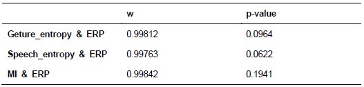
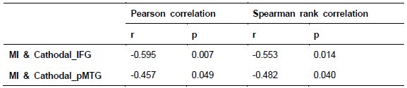
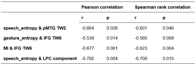
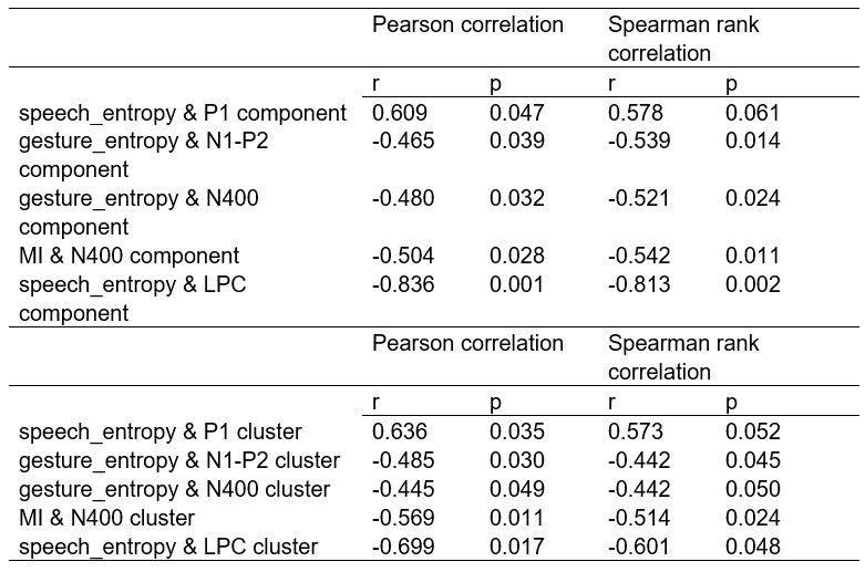
To further consolidate the relationship between entropy/MI and various ERP components, we also conducted a Spearman rank correlation analysis (Author response table 3-5). While the correlation between speech entropy and ERP amplitude in the P1 component yielded a p-value of 0.061, all other results were consistent with those obtained from the Pearson correlation analysis across the three experiments. Therefore, our conclusion that progressive neural responses reflected the degree of information remains robust. Although the Spearman rank and Pearson correlation analyses yielded similar results, we opted to report the Pearson correlation coefficients throughout the manuscript to maintain consistency.
Author response table 3.
Comparison of Pearson and Spearman results in Experiment 1
Author response table 4.
Comparison of Pearson and Spearman results in Experiment 2
Author response table 5.
Comparison of Pearson and Spearman results in Experiment 3
(2) Regarding the reviewer’s comment ‘choose to model the different variables to see whether MI/entropy could predict the neural responses’, we employed Representational Similarity Analysis (RSA) (Popal et.al, 2019) with MI and entropy as continuous variables. This analysis aimed to build a model to predict neural responses based on these feature metrics.
To capture dynamic temporal features indicative of different stages of multisensory integration, we segmented the EEG data into overlapping time windows (40 ms in duration with a 10 ms step size). The 40 ms window was chosen based on the TMS protocol used in Experiment 2, which also employed a 40 ms time window. The 10 ms step size (equivalent to 5 time points) was used to detect subtle shifts in neural responses that might not be captured by larger time windows, allowing for a more granular analysis of the temporal dynamics of neural activity.
Following segmentation, the EEG data were reshaped into a four-dimensional matrix (42 channels × 20 time points × 97 time windows × 20 features). To construct a neural similarity matrix, we averaged the EEG data across time points within each channel and each time window. The resulting matrix was then processed using the pdist function to compute pairwise distances between adjacent data points. This allowed us to calculate correlations between the neural matrix and three feature similarity matrices, which were constructed in a similar manner. These three matrices corresponded to (1) gesture entropy, (2) speech entropy, and (3) mutual information (MI). This approach enabled us to quantify how well the neural responses corresponded to the semantic dimensions of gesture and speech stimuli at each time window.
To determine the significance of the correlations between neural activity and feature matrices, we conducted 1000 permutation tests. In this procedure, we randomized the data or feature matrices and recalculated the correlations repeatedly, generating a null distribution against which the observed correlation values were compared. Statistical significance was determined if the observed correlation exceeded the null distribution threshold (p < 0.05). This permutation approach helps mitigate the risk of spurious correlations, ensuring that the relationships between the neural data and feature matrices are both robust and meaningful.
Finally, significant correlations were subjected to clustering analysis, which grouped similar neural response patterns across time windows and channels. This clustering allowed us to identify temporal and spatial patterns in the neural data that consistently aligned with the semantic features of gesture and speech stimuli, thus revealing the dynamic integration of these multisensory modalities across time. Results are as follows:
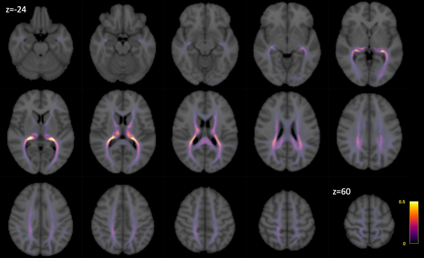
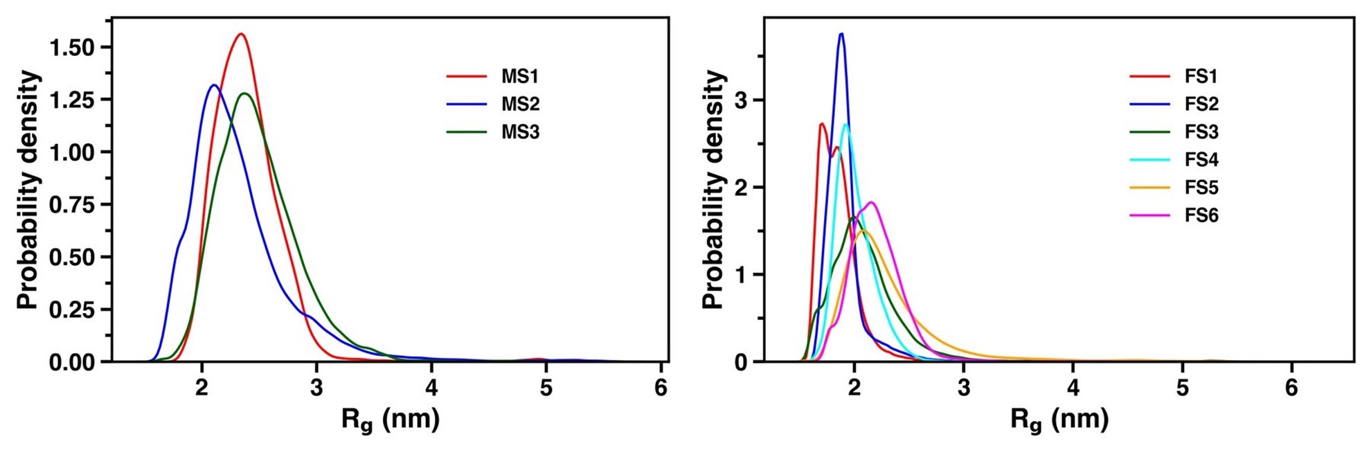
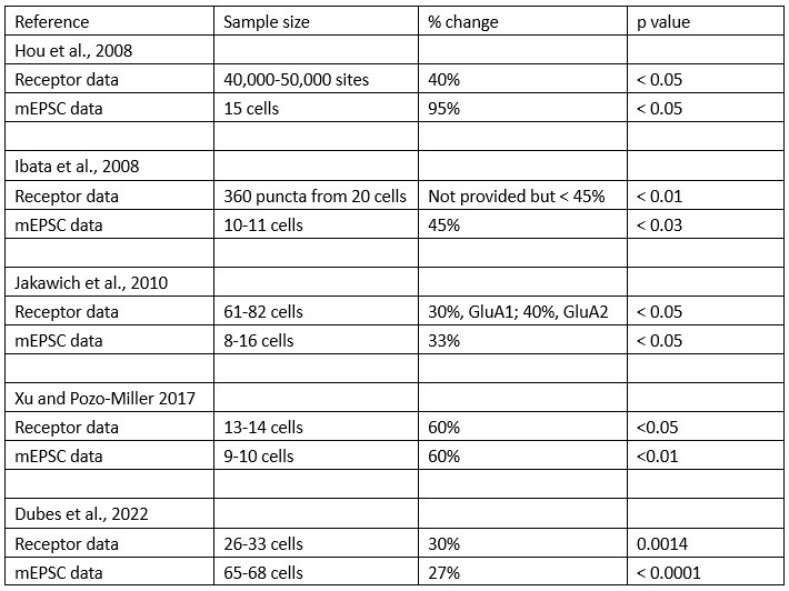
(1) Two significant clusters were identified for gesture entropy (Author response image 1 left). The first cluster was observed between 60-110 ms (channels F1 and F3), with correlation coefficients (r) ranging from 0.207 to 0.236 (p < 0.001). The second cluster was found between 210-280 ms (channel O1), with r-values ranging from 0.244 to 0.313 (p < 0.001).
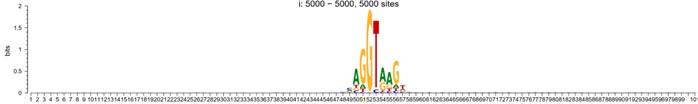
(2) For speech entropy (Author response image 1 middle), significant clusters were detected in both early and late time windows. In the early time windows, the largest significant cluster was found between 10-170 ms (channels F2, F4, F6, FC2, FC4, FC6, C4, C6, CP4, and CP6), with r-values ranging from 0.151 to 0.340 (p = 0.013), corresponding to the P1 component (0-100 ms). In the late time windows, the largest significant cluster was observed between 560-920 ms (across the whole brain, all channels), with r-values ranging from 0.152 to 0.619 (p = 0.013).
(3) For mutual information (MI) (Author response image 1 right), a significant cluster was found between 270-380 ms (channels FC1, FC2, FC3, FC5, C1, C2, C3, C5, CP1, CP2, CP3, CP5, FCz, Cz, and CPz), with r-values ranging from 0.198 to 0.372 (p = 0.001).
Author response image 1.
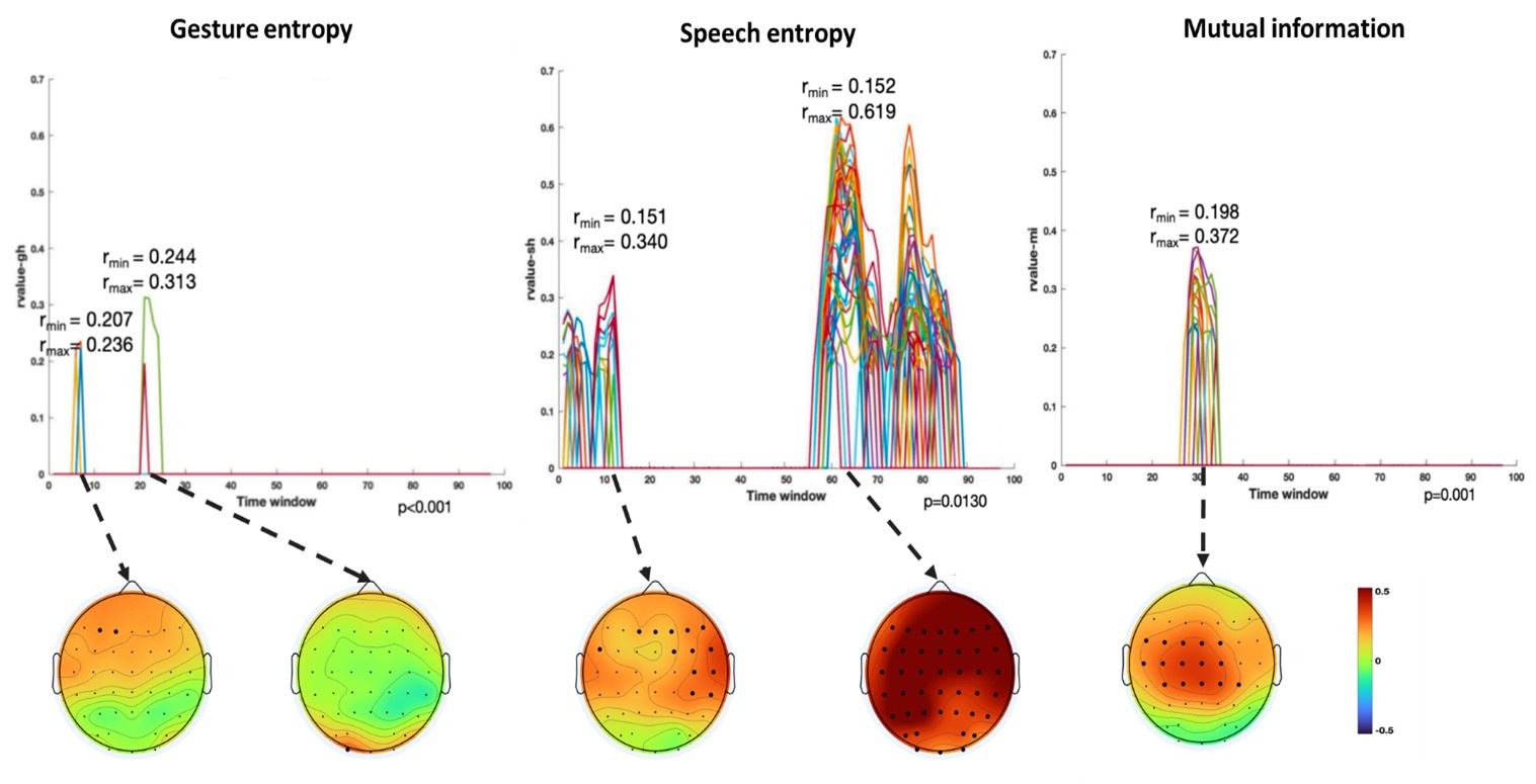
Results of RSA analysis.
These additional findings suggest that even using a different modeling approach, neural responses, as indexed by feature metrics of entropy and mutual information, are temporally aligned with distinct ERP components and ERP clusters, as reported in the current manuscript. This alignment serves to further consolidate the results, reinforcing the conclusion we draw. Considering the length of the manuscript, we did not include these results in the current manuscript.
(3) In terms of the correction of multiple comparisons, in Experiment 1, two separate participant groups were recruited for HD-tDCS applied over either the IFG or pMTG. FDR correction was performed separately for each group, resulting in six comparisons for each brain region (three information matrices × two tDCS effects: anodal-sham or cathodal-sham). In Experiment 2, six comparisons (three information matrices × two sites: IFG or pMTG) were submitted for FDR correction. In Experiment 3, FDR correction was applied to the seven regions of interest (ROIs) within each component, resulting in five comparisons.
Reference:
Wilk, M.B. (2015). The Shapiro Wilk And Related Tests For Normality.
Popal, H., Wang, Y., & Olson, I. R. (2019). A guide to representational similarity analysis for social neuroscience. Social cognitive and affective neuroscience, 14(11), 1243-1253.
(4) The authors use ROIs for their different analyses, but it is unclear why and on the basis of what these regions are defined. Why not consider all channels without making them part of an ROI, by using a method like the one described in my previous comment?
Response 4: For the EEG data, we conducted both a traditional ROI analysis and a cluster-based permutation approach. The ROIs were defined based on a well-established work (Habets et al., 2011), allowing for hypothesis-driven testing of specific regions. In addition, we employed a cluster-based permutation methods, which is data-driven and helps enhance robustness while addressing multiple comparisons. This method serves as a complement to the hypothesis-driven ROI analysis, offering an exploratory, unbiased perspective. Notably, the results from both approaches were consistent, reinforcing the reliability of our findings.
To make the methods more accessible to a broader audience, we clarified the relationship between these approaches in the revised manuscript in Lines 267-270: ‘To consolidate the data, we conducted both a traditional region-of-interest (ROI) analysis, with ROIs defined based on a well-established work40, and a cluster-based permutation approach, which utilizes data-driven permutations to enhance robustness and address multiple comparisons’
Additionally, we conducted an RSA analysis without defining specific ROIs, considering all channels in the analysis. This approach yielded consistent results, further validating the robustness of our findings across different analysis methods. See Response 3 for detail.
Reference:
Habets, B., Kita, S., Shao, Z.S., Ozyurek, A., and Hagoort, P. (2011). The Role of Synchrony and Ambiguity in Speech-Gesture Integration during Comprehension. J Cognitive Neurosci 23, 1845-1854. 10.1162/jocn.2010.21462
(5) The authors describe that they have divided their EEG data into a "lower half" and a "higher half" (lines 234-236), based on entropy scores. It is unclear why this is necessary, and I would suggest just using the entropy scores as a continuous measure.
Response 5: To identify ERP components or spatiotemporal clusters that demonstrated significant semantic differences, we split each model into higher and lower halves based on entropy scores. This division allowed us to capture distinct levels of information processing and explore how different levels of entropy or mutual information (MI) related to neural activity. Specifically, the goal was to highlight the gradual activation process of these components and clusters as they correlate with changes in information content. Remarkably, consistent results were observed between the ERP components and clusters, providing robust evidence that semantic information conveyed through gestures and speech significantly influenced the amplitude of these components or clusters. Moreover, the semantic information was shown to be highly sensitive, varying in tandem with these amplitude changes.
Reviewer #2 (Public review):
Comment:
Summary:
The study is an innovative and fundamental study that clarified important aspects of brain processes for integration of information from speech and iconic gesture (i.e., gesture that depicts action, movement, and shape), based on tDCS, TMS, and EEG experiments. They evaluated their speech and gesture stimuli in information-theoretic ways and calculated how informative speech is (i.e., entropy), how informative gesture is, and how much shared information speech and gesture encode. The tDCS and TMS studies found that the left IFG and pMTG, the two areas that were activated in fMRI studies on speech-gesture integration in the previous literature, are causally implicated in speech-gesture integration. The size of tDC and TMS effects are correlated with the entropy of the stimuli or mutual information, which indicates that the effects stem from the modulation of information decoding/integration processes. The EEG study showed that various ERP (event-related potential, e.g., N1-P2, N400, LPC) effects that have been observed in speech-gesture integration experiments in the previous literature, are modulated by the entropy of speech/gesture and mutual information. This makes it clear that these effects are related to information decoding processes. The authors propose a model of how the speech-gesture integration process unfolds in time, and how IFG and pMTG interact with each other in that process.
Strengths:
The key strength of this study is that the authors used information theoretic measures of their stimuli (i.e., entropy and mutual information between speech and gesture) in all of their analyses. This made it clear that the neuro-modulation (tDCS, TMS) affected information decoding/integration and ERP effects reflect information decoding/integration. This study used tDCS and TMS methods to demonstrate that left IFG and pMTG are causally involved in speech-gesture integration. The size of tDCS and TMS effects are correlated with information-theoretic measures of the stimuli, which indicate that the effects indeed stem from disruption/facilitation of the information decoding/integration process (rather than generic excitation/inhibition). The authors' results also showed a correlation between information-theoretic measures of stimuli with various ERP effects. This indicates that these ERP effects reflect the information decoding/integration process.
We sincerely thank the reviewer for recognizing our efforts and the innovation of employing information-theoretic measures to elucidate the brain processes underlying the multisensory integration of gesture and speech.
Weaknesses:
The "mutual information" cannot fully capture the interplay of the meaning of speech and gesture. The mutual information is calculated based on what information can be decoded from speech alone and what information can be decoded from gesture alone. However, when speech and gesture are combined, a novel meaning can emerge, which cannot be decoded from a single modality alone. When example, a person produces a gesture of writing something with a pen, while saying "He paid". The speech-gesture combination can be interpreted as "paying by signing a cheque". It is highly unlikely that this meaning is decoded when people hear speech only or see gestures only. The current study cannot address how such speech-gesture integration occurs in the brain, and what ERP effects may reflect such a process. Future studies can classify different types of speech-gesture integration and investigate neural processes that underlie each type. Another important topic for future studies is to investigate how the neural processes of speech-gesture integration change when the relative timing between the speech stimulus and the gesture stimulus changes.
We greatly appreciate Reviewer2 ’s thoughtful concern regarding whether "mutual information" adequately captures the interplay between the meanings of speech and gesture. We would like to clarify that the materials used in the present study involved gestures that were performed without actual objects, paired with verbs that precisely describe the corresponding actions. For example, a hammering gesture was paired with the verb “hammer”, and a cutting gesture was paired with the verb “cut”. In this design, all gestures conveyed redundant information relative to the co-occurring speech, creating significant overlap between the information derived from speech alone and that from gesture alone.
We understand the reviewer’s concern about cases where gestures and speech might provide complementary, rather than redundant, information. To address this, we have developed an alternative metric for quantifying information gains contributed by supplementary multisensory cues, which will be explored in a subsequent study. However, for the present study, we believe that the observed overlap in information serves as a key indicator of multisensory convergence, a central focus of our investigation.
Regarding the reviewer’s concern about how neural processes of speech-gesture integration may change with varying relative timing between speech and gesture stimuli, we would like to highlight findings from our previous study (Zhao, 2023, Frontiers in Psychology). In that study, we explored the semantic predictive role of gestures relative to speech under two timing conditions: (1) gestures preceding speech by a fixed interval of 200 ms, and (2) gestures preceding speech at its semantic identification point. Interestingly, only in the second condition did we observe time-window-selective disruptions of the semantic congruency effect in the IFG and pMTG. This led us to conclude that gestures play a semantic priming role for co-occurring speech. Building on this, we designed the present study with gestures deliberately preceding speech at its semantic identification point to reflect this semantic priming relationship. Additionally, ongoing research in our lab is exploring gesture and speech interactions in natural conversational settings to investigate whether the neural processes identified here remain consistent across varying contexts.
To address potential concerns and ensure clarity regarding the limitations of the MI measurement, we have included a discussion of tthis in the revised manuscript in Lines 543-547: ‘Furthermore, MI quantifies overlap in gesture-speech integration, primarily when gestures convey redundant meaning. Consequently, the conclusions drawn in this study are constrained to contexts in which gestures serve to reinforce the meaning of the speech. Future research should aim to explore the neural responses in cases where gestures convey supplementary, rather than redundant, semantic information.’ This is followed by a clarification of the timing relationship between gesture and speech: ‘Note that the sequential cortical involvement and ERP components discussed above are derived from a deliberate alignment of speech onset with gesture DP, creating an artificial priming effect with gesture semantically preceding speech. Caution is advised when generalizing these findings to the spontaneous gesture-speech relationships, although gestures naturally precede speech[34].’ (Lines 539-543).
Reviewer #3 (Public review):
In this useful study, Zhao et al. try to extend the evidence for their previously described two-step model of speech-gesture integration in the posterior Middle Temporal Gyrus (pMTG) and Inferior Frontal Gyrus (IFG). They repeat some of their previous experimental paradigms, but this time quantifying Information-Theoretical (IT) metrics of the stimuli in a stroop-like paradigm purported to engage speech-gesture integration. They then correlate these metrics with the disruption of what they claim to be an integration effect observable in reaction times during the tasks following brain stimulation, as well as documenting the ERP components in response to the variability in these metrics.
The integration of multiple methods, like tDCS, TMS, and ERPs to provide converging evidence renders the results solid. However, their interpretation of the results should be taken with care, as some critical confounds, like difficulty, were not accounted for, and the conceptual link between the IT metrics and what the authors claim they index is tenuous and in need of more evidence. In some cases, the difficulty making this link seems to arise from conceptual equivocation (e.g., their claims regarding 'graded' evidence), whilst in some others it might arise from the usage of unclear wording in the writing of the manuscript (e.g. the sentence 'quantitatively functional mental states defined by a specific parser unified by statistical regularities'). Having said that, the authors' aim is valuable, and addressing these issues would render the work a very useful approach to improve our understanding of integration during semantic processing, being of interest to scientists working in cognitive neuroscience and neuroimaging.
The main hurdle to achieving the aims set by the authors is the presence of the confound of difficulty in their IT metrics. Their measure of entropy, for example, being derived from the distribution of responses of the participants to the stimuli, will tend to be high for words or gestures with multiple competing candidate representations (this is what would presumptively give rise to the diversity of responses in high-entropy items). There is ample evidence implicating IFG and pMTG as key regions of the semantic control network, which is critical during difficult semantic processing when, for example, semantic processing must resolve competition between multiple candidate representations, or when there are increased selection pressures (Jackson et al., 2021). Thus, the authors' interpretation of Mutual Information (MI) as an index of integration is inextricably contaminated with difficulty arising from multiple candidate representations. This casts doubt on the claims of the role of pMTG and IFG as regions carrying out gesture-speech integration as the observed pattern of results could also be interpreted in terms of brain stimulation interrupting the semantic control network's ability to select the best candidate for a given context or respond to more demanding semantic processing.
Response 1: We sincerely thank the reviewer for pointing out the confound of difficulty. The primary aim of this study is to investigate whether the degree of activity in the established integration hubs, IFG and pMTG, is influenced by the information provided by gesture-speech modalities and/or their interactions. While we provided evidence for the differential involvement of the IFG and pMTG by delineating their dynamic engagement across distinct time windows of gesture-speech integration and associating these patterns with unisensory information and their interaction, we acknowledge that the mechanisms underlying these dynamics remain open to interpretation. Specifically, whether the observed effects stem from difficulties in semantic control processes, as suggested by the reviewer, or from resolving information uncertainty, as quantified by entropy, falls outside the scope of the current study. Importantly, we view these two interpretations as complementary rather than mutually exclusive, as both may be contributing factors. Nonetheless, we agree that addressing this question is a compelling avenue for future research.
In the revised manuscript, we have included an additional analysis to assess whether the confounding effects of lexical or semantic control difficulty—specifically, the number of available responses—affect the neural outcomes. To address this, we performed partial correlation analyses, controlling for the number of responses.
We would like to clarify an important distinction between the measure of entropy derived from the distribution of responses and the concept of response diversity. Entropy, in our analysis, is computed based on the probability distribution of each response, as captured by the information entropy formula. In contrast, response diversity refers to the simple count of different responses provided. Mutual Information (MI), by its nature, is also an entropy measure, quantifying the overlap in responses. For reference, although we observed a high correlation between the three information matrices and the number of responses (gesture entropy & gesture response number: r = 0.976, p < 0.001; speech entropy & speech response number: r = 0.961, p < 0.001; MI & total response number: r = 0.818, p < 0.001), it is crucial to emphasize that these metrics capture different aspects of the semantic information represented. In the revised manuscript, we have provided a table detailing both entropy and response numbers for each stimulus, to allow for greater transparency and clarity.
Furthermore, we have added a comprehensive description of the partial correlation analysis conducted across all three experiments in the methodology section: for Experiment 1, please refer to Lines 213–222: ‘To account for potential confounds related to multiple candidate representations, we conducted partial correlation analyses between the tDCS effects and gesture entropy, speech entropy, and MI, controlling for the number of responses provided for each gesture and speech, as well as the total number of combined responses. Given that HD-tDCS induces overall disruption at the targeted brain regions, we hypothesized that the neural activity within the left IFG and pMTG would be progressively affected by varying levels of multisensory convergence, as indexed by MI. Moreover, we hypothesized that the modulation of neural activity by MI would differ between the left IFG and pMTG, as reflected in the differential modulation of response numbers in the partial correlations, highlighting their distinct roles in semantic processing[37].’
Experiment 2: ‘To control for potential confounds, partial correlations were also performed between the TMS effects and gesture entropy, speech entropy, and MI, controlling for the number of responses for each gesture and speech, as well as the total number of combined responses. By doing this, we can determine how the time-sensitive contribution of the left IFG and pMTG to gesture–speech integration was affected by gesture and speech information distribution.’ (Lines 242–246).
Experiment 3: ‘Additionally, partial correlations were conducted, accounting for the number of responses for each respective metric’ (Lines 292–293).
As anticipated by the reviewer, we observed a consistent modulation of response numbers across both regions as well as across the four ERP components and associated clusters. The detailed results are presented below:
Experiment 1: ‘However, partial correlation analysis, controlling for the total response number, revealed that the initially significant correlation between the Cathodal-tDCS effect and MI was no longer significant (r = -0.303, p = 0.222, 95% CI = [-0.770, 0.164]). This suggests that the observed relationship between Cathodal-tDCS and MI may be confounded by semantic control difficulty, as reflected by the total number of responses. Specifically, the reduced activity in the IFG under Cathodal-tDCS may be driven by variations in the difficulty of semantic control rather than a direct modulation of MI.’ (Lines 310-316) and ‘’Importantly, the reduced activity in the pMTG under Cathodal-tDCS was not influenced by the total response number, as indicated by the non-significant correlation (r = -0.253, p = 0.295, 95% CI = [-0.735, 0.229]). This finding was further corroborated by the unchanged significance in the partial correlation between Cathodal-tDCS and MI, when controlling for the total response number (r = -0.472, p = 0.048, 95% CI = [-0.903, -0.041]). (Lines 324-328).
Experiment 2:’ Notably, inhibition of pMTG activity in TW2 was not influenced by the number of speech responses (r = -0.539, p = 0.087, 95% CI = [-1.145, 0.067]). However, the number of speech responses did affect the modulation of speech entropy on the pMTG inhibition effect in TW2. This was evidenced by the non-significant partial correlation between pMTG inhibition and speech entropy when controlling for speech response number (r = -0.218, p = 0.545, 95% CI = [-0.563, 0.127]).
In contrast, the interrupted IFG activity in TW6 appeared to be consistently influenced by the confound of semantic control difficulty. This was reflected in the significant correlation with both gesture response number (r = -0.480, p = 0.032, 95% CI = [-904, -0.056]), speech response number (r = -0.729, p = 0.011, 95% CI = [-1.221, -0.237]), and total response number (r = -0.591, p = 0.008, 95% CI = [-0.993, -0.189]). Additionally, partial correlation analyses revealed non-significant relationship between interrupted IFG activity in TW6 and gesture entropy (r = -0.369, p = 0.120, 95% CI = [-0.810, -0.072]), speech entropy (r = -0.455, p = 0.187, 95% CI = [-1.072, 0.162]), and MI (r = -0.410, p = 0.091, 95% CI = [-0.856, -0.036]) when controlling for response numbers.’ (Lines 349-363)
Experiment 3: ‘To clarify potential confounds of semantic control difficulty, partial correlation analyses were conducted to examine the relationship between the elicited ERP components and the relevant information matrices, controlling for response numbers. Results consistently indicated modulation by response numbers in the relationship of ERP components with the information matrix, as evidenced by the non-significant partial correlations between the P1 amplitude (P1 component over ML: r = -0.574, p = 0.082, 95% CI = [-1.141, -0.007]) and the P1 cluster (r = -0.503, p = 0.138, 95% CI = [-1.102, 0.096]) with speech entropy; the N1-P2 amplitude (N1-P2 component over LA: r = -0.080, p = 0.746, 95% CI = [-0.554, 0.394]) and N1-P2 cluster (r \= -0.179, p = 0.464, 95% CI = [-0.647, 0.289]) with gesture entropy; the N400 amplitude (N400 component over LA: r = 0.264, p = 0.247, 95% CI = [-0.195,0.723]) and N400 cluster (r = 0.394, p = 0.095, 95% CI = [-0.043, 0.831]) with gesture entropy; the N400 amplitude (N400 component over LA: r = -0.134, p = 0.595, 95% CI = [-0.620, 0.352]) and N400 cluster (r = -0.034, p = 0.894, 95% CI = [-0.524,0.456]) with MI; and the LPC amplitude (LPC component over LA: r \= -0.428, p = 0.217, 95% CI = [-1.054, 0.198]) and LPC cluster (r \= -0.202, p = 0.575, 95% CI = [-0.881, 0.477]) with speech entropy.’ (Lines 424-438)
Based on the above results, we conclude that there is a dynamic interplay between the difficulty of semantic representation and the control pressures that shape the resulting neural responses. Furthermore, while the role of the IFG in control processes remains consistent, the present study reveals a more segmented role for the pMTG. Specifically, although the pMTG is well-established in the processing of distributed speech information, the integration of multisensory convergence, as indexed by MI, did not elicit the same control-related modulation in pMTG activity. A comprehensive discussion of the control process in shaping neural responses, as well as the specific roles of the IFG and pMTG in this process, is provided in the Discussion section in Lines (493-511): ‘Given that control processes are intrinsically integrated with semantic processing50, a distributed semantic representation enables dynamic modulation of access to and manipulation of meaningful information, thereby facilitating flexible control over the diverse possibilities inherent in a concept. Accordingly, an increased number of candidate responses amplifies the control demands necessary to resolve competing semantic representations. This effect was observed in the present study, where the association of the information matrix with the tDCS effect in IFG, the inhibition of pMTG activity in TW2, disruption of IFG activity in TW6, and modulation of four distinct ERP components collectively demonstrated that response quantity modulated neural activity. These results underscore the intricate interplay between the difficulty of semantic representation and the control pressures that shape the resulting neural responses.
The IFG and pMTG, central components of the semantic control network, have been extensively implicated in previous research 50-52. While the role of the IFG in managing both unisensory information and multisensory convergence remains consistent, as evidenced by the confounding difficulty results across Experiments 1 and 2, the current study highlights a more context-dependent function for the pMTG. Specifically, although the pMTG is well-established in the processing of distributed speech information, the multisensory convergence, indexed by MI, did not evoke the same control-related modulation in pMTG activity. These findings suggest that, while the pMTG is critical to semantic processing, its engagement in control processes is likely modulated by the specific nature of the sensory inputs involved’
Reference:
Tesink, C.M.J.Y., Petersson, K.M., van Berkum, J.J.A., van den Brink, D., Buitelaar, J.K., and Hagoort, P. (2009). Unification of speaker and meaning in language comprehension: An fMRI study. J Cognitive Neurosci 21, 2085-2099. 10.1162/jocn.2008.21161
Jackson, R.L. (2021). The neural correlates of semantic control revisited. Neuroimage 224, 117444. 10.1016/j.neuroimage.2020.117444.
Jefferies, E. (2013). The neural basis of semantic cognition: converging evidence from neuropsychology, neuroimaging and TMS. Cortex 49, 611-625. 10.1016/j.cortex.2012.10.008.
Noonan, K.A., Jefferies, E., Visser, M., and Lambon Ralph, M.A. (2013). Going beyond inferior prefrontal involvement in semantic control: evidence for the additional contribution of dorsal angular gyrus and posterior middle temporal cortex. J Cogn Neurosci 25, 1824-1850. 10.1162/jocn_a_00442.
In terms of conceptual equivocation, the use of the term 'graded' by the authors seems to be different from the usage commonly employed in the semantic cognition literature (e.g., the 'graded hub hypothesis', Rice et al., 2015). The idea of a graded hub in the controlled semantic cognition framework (i.e., the anterior temporal lobe) refers to a progressive degree of abstraction or heteromodal information as you progress through the anatomy of the region (i.e., along the dorsal-to-ventral axis). The authors, on the other hand, seem to refer to 'graded manner' in the context of a correlation of entropy or MI and the change in the difference between Reaction Times (RTs) of semantically congruent vs incongruent gesture-speech. The issue is that the discourse through parts of the introduction and discussion seems to conflate both interpretations, and the ideas in the main text do not correspond to the references they cite. This is not overall very convincing. What is it exactly the authors are arguing about the correlation between RTs and MI indexes? As stated above, their measure of entropy captures the spread of responses, which could also be a measure of item difficulty (more diverse responses imply fewer correct responses, a classic index of difficulty). Capturing the diversity of responses means that items with high entropy scores are also likely to have multiple candidate representations, leading to increased selection pressures. Regions like pMTG and IFG have been widely implicated in difficult semantic processing and increased selection pressures (Jackson et al., 2021). How is this MI correlation evidence of integration that proceeds in a 'graded manner'? The conceptual links between these concepts must be made clearer for the interpretation to be convincing.
Response 2: Regarding the concern of conceptual equivocation, we would like to emphasize that this study represents the first attempt to focus on the relationship between information quantity and neural engagement, a question addressed in three experiments. Experiment 1 (HD-tDCS) targeted the entire gesture-speech integration process in the IFG and pMTG to assess whether neural activity in these regions, previously identified as integration hubs, is modulated by changes in informativeness from both modalities (i.e., entropy) and their interactions (MI). The results revealed a gradual inhibition of neural activity in both areas as MI increased, evidenced by a negative correlation between MI and the tDCS inhibition effect in both regions. Building on this, Experiments 2 and 3 employed double-pulse TMS and ERPs to further assess whether the engaged neural activity was both time-sensitive and staged. These experiments also evaluated the contributions of various sources of information, revealing correlations between information-theoretic metrics and time-locked brain activity, providing insights into the ‘gradual’ nature of gesture-speech integration.
Therefore, the incremental engagement of the integration hub of IFG and pMTG along with the informativeness of gesture and speech during multisensory integration is different from the "graded hub," which refers to anatomical distribution. We sincerely apologize for this oversight. In the revised manuscript, we have changed the relevant conceptual equivocation in Lines 44-60: ‘Consensus acknowledges the presence of 'convergence zones' within the temporal and inferior parietal areas [1], or the 'semantic hub' located in the anterior temporal lobe[2], pivotal for integrating, converging, or distilling multimodal inputs. Contemporary theories frame the semantic processing as a dynamic sequence of neural states[3], shaped by systems that are finely tuned to the statistical regularities inherent in sensory inputs[4]. These regularities enable the brain to evaluate, weight, and integrate multisensory information, optimizing the reliability of individual sensory signals[5]. However, sensory inputs available to the brain are often incomplete and uncertain, necessitating adaptive neural adjustments to resolve these ambiguities [6]. In this context, neuronal activity is thought to be linked to the probability density of sensory information, with higher levels of uncertainty resulting in the engagement of a broader population of neurons, thereby reflecting the brain’s adaptive capacity to handle diverse possible interpretations[7,8]. Although the role of 'convergence zones' and 'semantic hubs' in integrating multimodal inputs is well established, the precise functional patterns of neural activity in response to the distribution of unified multisensory information—along with the influence of unisensory signals—remain poorly understood.
To this end, we developed an analytic approach to directly probe the cortical engagement during multisensory gesture-speech semantic integration.’
Furthermore, in the Discussion section, we have replaced the term 'graded' with 'incremental' (Line 456,). Additionally, we have included a discussion on the progressive nature of neural engagement, as evidenced by the correlation between RTs and MI indices in Lines 483-492: ‘The varying contributions of unisensory gesture-speech information and the convergence of multisensory inputs, as reflected in the correlation between distinct ERP components and TMS time windows (TMS TWs), are consistent with recent models suggesting that multisensory processing involves parallel detection of modality-specific information and hierarchical integration across multiple neural levels[4,48]. These processes are further characterized by coordination across multiple temporal scales[49]. Building on this, the present study offers additional evidence that the multi-level nature of gesture-speech processing is statistically structured, as measured by information matrix of unisensory entropy and multisensory convergence index of MI, the input of either source would activate a distributed representation, resulting in progressively functioning neural responses.’
Reference:
Damasio, H., Grabowski, T.J., Tranel, D., Hichwa, R.D., and Damasio, A.R. (1996). A neural basis for lexical retrieval. Nature 380, 499-505. DOI 10.1038/380499a0.
Patterson, K., Nestor, P.J., and Rogers, T.T. (2007). Where do you know what you know? The representation of semantic knowledge in the human brain. Nature Reviews Neuroscience 8, 976-987. 10.1038/nrn2277.
Brennan, J.R., Stabler, E.P., Van Wagenen, S.E., Luh, W.M., and Hale, J.T. (2016). Abstract linguistic structure correlates with temporal activity during naturalistic comprehension. Brain and Language 157, 81-94. 10.1016/j.bandl.2016.04.008.
Benetti, S., Ferrari, A., and Pavani, F. (2023). Multimodal processing in face-to-face interactions: A bridging link between psycholinguistics and sensory neuroscience. Front Hum Neurosci 17, 1108354. 10.3389/fnhum.2023.1108354.
Noppeney, U. (2021). Perceptual Inference, Learning, and Attention in a Multisensory World. Annual Review of Neuroscience, Vol 44, 2021 44, 449-473. 10.1146/annurev-neuro-100120-085519.
Ma, W.J., and Jazayeri, M. (2014). Neural coding of uncertainty and probability. Annu Rev Neurosci 37, 205-220. 10.1146/annurev-neuro-071013-014017.
Fischer, B.J., and Pena, J.L. (2011). Owl's behavior and neural representation predicted by Bayesian inference. Nat Neurosci 14, 1061-1066. 10.1038/nn.2872.
Ganguli, D., and Simoncelli, E.P. (2014). Efficient sensory encoding and Bayesian inference with heterogeneous neural populations. Neural Comput 26, 2103-2134. 10.1162/NECO_a_00638.
Meijer, G.T., Mertens, P.E.C., Pennartz, C.M.A., Olcese, U., and Lansink, C.S. (2019). The circuit architecture of cortical multisensory processing: Distinct functions jointly operating within a common anatomical network. Prog Neurobiol 174, 1-15. 10.1016/j.pneurobio.2019.01.004.
Senkowski, D., and Engel, A.K. (2024). Multi-timescale neural dynamics for multisensory integration. Nat Rev Neurosci 25, 625-642. 10.1038/s41583-024-00845-7.
Reviewer #2 (Recommendations for the authors):
I have a number of small suggestions to make the paper more easy to understand.
We sincerely thank the reviewer for their careful reading and thoughtful consideration. All suggestions have been thoroughly addressed and incorporated into the revised manuscript.
(1) Lines 86-87, please clarify whether "chronometric double-pulse TMS" should lead to either excitation or inhibition of neural activities
Double-pulse TMS elicits inhibition of neural activities (see responses to editors), which has been clarified in the revised manuscript in Lines 90-93: ‘we applied inhibitory chronometric double-pulse transcranial magnetic stimulation (TMS) to specific temporal windows associated with integration processes in these regions[23], assessing whether the inhibitory effects of TMS were correlated with unisensory entropy or the multisensory convergence index (MI)’
(2) Line 106 "validated by replicating the semantic congruencey effect". Please specify what the task was in the validation study.
The description of the validation task has been added in Lines 116-119: ‘To validate the stimuli, 30 participants were recruited to replicate the multisensory index of semantic congruency effect, hypothesizing that reaction times for semantically incongruent gesture-speech pairs would be significantly longer than those for congruent pairs.’
(3) Line 112. "30 subjects". Are they Chinese speakers?
Yes, all participants in the present study, including those in the pre-tests, are native Chinese speakers.
(4) Line 122, "responses for each item" Please specify whether you mean here "the comprehensive answer" as you defined in 118-119.
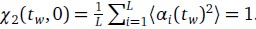
Yes, and this information has been added in Lines 136-137: ‘comprehensive responses for each item were converted into Shannon's entropy (H)’
(5) Line 163 "one of three stimulus types (Anodal, Cathodal or Sham)". Please specify whether the order of the three conditions was counterbalanced across participants. Or, whether the order was fixed for all participants.
The order of the three conditions was counterbalanced across participants, a clearer description has been added in the revised manuscript in Lines 184-189: ‘Participants were divided into two groups, with each group undergoing HD-tDCS stimulation at different target sites (IFG or pMTG). Each participant completed three experimental sessions, spaced one week apart, during which 480 gesture-speech pairs were presented across various conditions. In each session, participants received one of three types of HD-tDCS stimulation: Anodal, Cathodal, or Sham. The order of stimulation site and type was counterbalanced using a Latin square design to control for potential order effects.’
(6) Line 191-192, "difference in reaction time between semantic incongruence and semantic congruent pairs)" Here, please specify which reaction time was subtracted from which one. This information is very crucial; without it, you cannot interpret your graphs.
(17) Figure 3. Figure caption for (A). "The semantic congruence effect was calculated as the reaction time difference between...". You need to specify which condition was subtracted from what condition; otherwise, you cannot interpret this figure. "difference" is too ambiguous.
Corrections have been made in the revised manuscript in Lines 208-211: ‘Neural responses were quantified based on the effects of HD-tDCS (active tDCS minus sham tDCS) on the semantic congruency effect, defined as the difference in reaction times between semantic incongruent and congruent conditions (Rt(incongruent) - Rt(congruent))’ and Line 796-798: ‘The semantic congruency effect was calculated as the reaction time (RT) difference between semantically incongruent and semantically congruent pairs (Rt(incongruent) - Rt(congruent))’.
(7) Line 363 "progressive inhibition of IFG and pMTG by HD-tDCS as the degree of gesture-speech interaction, indexed by MI, advanced." This sentence is very hard to follow. I don't understand what part of the data in Figure 3 speaks to "inhibition of IFG". And what is "HD-tDCS"? I think it is easier to read if you talk about correlation (not "progressive" and "advanced").
High-Definition transcranial direct current stimulation (HD-tDCS) was applied to modulate the activity of pMTG and IFG, with cathodal stimulation inducing inhibitory effects and anodal stimulation facilitating neural activity. In Figure 3, we examined the relationship between the tDCS effects on pMTG and IFG and the three information matrices (entropy and MI). Our results revealed significant correlations between MI and the cathodal-tDCS effects in both regions. We acknowledge that the original phrasing may have been unclear, and in the revised manuscript, we have provided a more explicit explanation to enhance clarity in Lines 443-445: ‘Our results, for the first time, revealed that the inhibition effect of cathodal-tDCS on the pMTG and IFG correlated with the degree of gesture-speech multisensory convergence, as indexed by MI’.
(8) Lines 367-368 I don't understand why gesture is top down and speech is bottom up. Is that because gesture precedes speech (gesture is interpretable at the point of speech onset)?
Yes, since we employed a semantic priming paradigm by aligning speech onset with the gesture comprehension point, we interpret the gesture-speech integration process as an interaction between the top-down prediction from gestures and the bottom-up processing of speech. In the revised manuscript, we have provided a clearer and more coherent description that aligns with the results. Lines 445-449: ‘Moreover, the gradual neural engagement was found to be time-sensitive and staged, as evidenced by the selectively interrupted time windows (Experiment 2) and the distinct correlated ERP components (Experiment 3), which were modulated by different information contributors, including unisensory entropy or multisensory MI’
(9) Line 380 - 381. Can you spell out "TW" and "IP"?
(16) Line 448, NIBS, Please spell out "NIBS".
"TW" have been spelled out in Lines 459: ‘time windows (TW)’,"IP" in Line 460: ‘identification point (IP)’. The term "NIBS" was replaced with "HD-tDCS and TMS" to provide clearer specification of the techniques employed: ‘Consistent with this, the present study provides robust evidence, through the application of HD-tDCS and TMS, that the integration hubs for gesture and speech—the pMTG and IFG—operate in an incremental manner.’ (Lines 454-457).
(10) Line 419, The higher certainty of gesture => The higher the certainty of gesture is
(13) Line 428, "a larger MI" => "a larger MI is"
(12) Line 427-428, "the larger overlapped neural populations" => "the larger, the overlapped neural populations"
Changes have been made in Line 522 ‘The higher the certainty of gesture is’ , Line 531: ‘a larger MI is’ and Line 530 ‘the larger, overlapped neural populations’
(11) Line 423 "Greater TMS effect over the IFG" Can you describe the TMS effect?
TMS effect has been described as ‘Greater TMS inhibitory effect’ (Line 526)
(14) Line 423 "reweighting effect" What is this? Please describe (and say which experiment it is about).
Clearer description has been provided in Lines 535-538: ‘As speech entropy increases, indicating greater uncertainty in the information provided by speech, more cognitive effort is directed towards selecting the targeted semantic representation. This leads to enhanced involvement of the IFG and a corresponding reduction in LPC amplitude’.
(15) Line 437 "the graded functionality of every disturbed period is not guaranteed" (I don't understand this sentence).
Clearer description has been provided in Lines 552-557: ‘Additionally, not all influenced TWs exhibited significant associations with entropy and MI. While HD-tDCS and TMS may impact functionally and anatomically connected brain regions[55,56], whether the absence of influence in certain TWs can be attributed to compensation by other connected brain areas, such as angular gyrus[57] or anterior temporal lobe[58], warrants further investigation. Therefore, caution is needed when interpreting the causal relationship between inhibition effects of brain stimulation and information-theoretic metrics (entropy and MI).’
References:
Humphreys, G. F., Lambon Ralph, M. A., & Simons, J. S. (2021). A Unifying Account of Angular Gyrus Contributions to Episodic and Semantic Cognition. Trends in neurosciences, 44(6), 452–463. https://doi.org/10.1016/j.tins.2021.01.006
Bonner, M. F., & Price, A. R. (2013). Where is the anterior temporal lobe and what does it do?. The Journal of neuroscience : the official journal of the Society for Neuroscience, 33(10), 4213–4215. https://doi.org/10.1523/JNEUROSCI.0041-13.2013
(18) Figure 4. "TW1", "TW2", etc. are not informative. Either replace them with the actual manuscript or add manuscript information (either in the graph itself or in the figure title).
Information was added into the figure title ‘Figure 4. TMS impacts on semantic congruency effect across various time windows (TW).’ (Line 804), included a detailed description of each time window in Lines 805-807: ‘(A) Five time windows (TWs) showing selective disruption of gesture-speech integration were chosen: TW1 (-120 to -80 ms relative to speech identification point), TW2 (-80 to -40 ms), TW3 (-40 to 0 ms), TW6 (80 to 120 ms), and TW7 (120 to 160 ms).’
(19) Table 2C.
The last column is titled "p(xi, yi)". I don't understand why the authors use this label for this column.
In the formula, at the very end, there is "p(xi|yi). I wonder why it is p(xi|yi), as opposed to p(yi|xi).
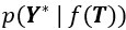
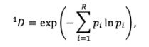
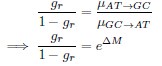
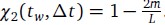
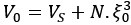
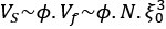
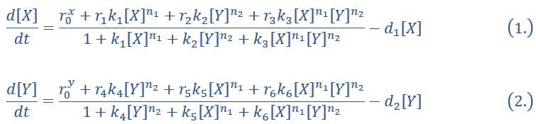
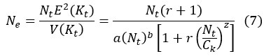
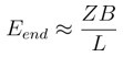
Mutual Information (MI) was calculated by subtracting the entropy of the combined gesture-speech dataset (Entropy(gesture + speech)) from the sum of the individual entropies of gesture and speech (Entropy(gesture) + Entropy(speech)). Thus, the p(xi,yi) aimed to describe the entropy of the combined dataset. We acknowledge the potential ambiguity in the original description, and in the revised manuscript, we have changed the formula of p(xi,yi) into ‘p(xi+yi)’ (Line 848) in Table 2C, and the relevant equation of MI ‘ ’. Also we provided a clear MI calculation process in Lines 143-146: ‘MI was used to measure the overlap between gesture and speech information, calculated by subtracting the entropy of the combined gesture-speech dataset (Entropy(gesture + speech)) from the sum of their individual entropies (Entropy(gesture) + Entropy(speech)) (see Appendix Table 2C)’.
Reviewer #3 (Recommendations for the authors):
(1) The authors should try and produce data showing that the confound of difficulty due to the number of lexical or semantic representations is not underlying high-entropy items if they wish to improve the credibility of their claim that the disruption of the congruency effect is due to speech-gesture integration. Additionally, they should provide more evidence either in the form of experiments or references to better justify why mutual information is an index for integration in the first place.
Response 1: An additional analysis has been conducted to assess whether the number of lexical or semantic representations affect the neural outcomes, please see details in the Responses to Reviewer 3 (public review) response 1.
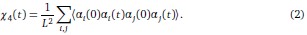
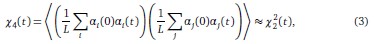
Mutual information (MI), a concept rooted in information theory, quantifies the reduction in uncertainty about one signal when the other is known, thereby capturing the statistical dependence between them. MI is calculated as the difference between the individual entropies of each signal and their joint entropy, which reflects the total uncertainty when both signals are considered together. This metric aligns with the core principle of multisensory integration: different modalities reduce uncertainty about each other by providing complementary, predictive information. Higher MI values signify that the integration of sensory signals results in a more coherent and unified representation, while lower MI values indicate less integration or greater divergence between the modalities. As such, MI serves as a robust and natural index for assessing the degree of multisensory integration.
To date, the use of MI as an index of integration has been limited, with one notable study by Tremblay et al. (2016), cited in the manuscript, using pointwise MI to quantify the extent to which two syllables mutually constrain each other. While MI has been extensively applied in natural language processing to measure the co-occurrence strength between words (e.g., Lin et al., 2012), its application as an index of multisensory convergence—particularly in the context of gesture-speech integration as employed in this study—is novel. In the revised manuscript, we have clarified the relationship between MI and multisensory convergence: ‘MI assesses share information between modalities[25],indicating multisensory convergence and acting as an index of gesture-speech integration’ (Lines 73-74).
Also, in our study, we calculated MI as per its original definition, by subtracting the entropy of summed dataset of gesture-speech from the combined entropies of gesture and speech. The detailed calculation method is provided in Lines 136-152: ‘To quantify information content, comprehensive responses for each item were converted into Shannon's entropy (H) as a measure of information richness (Figure 1A bottom). With no significant gender differences observed in both gesture (t(20) = 0.21, p = 0.84) and speech (t(20) = 0.52, p = 0.61), responses were aggregated across genders, resulting in 60 answers per item (Appendix Table 2). Here, p(xi) and p(yi) represent the distribution of 60 answers for a given gesture (Appendix Table 2B) and speech (Appendix Table 2A), respectively. High entropy indicates diverse answers, reflecting broad representation, while low entropy suggests focused lexical recognition for a specific item (Figure 2B). MI was used to measure the overlap between gesture and speech information, calculated by subtracting the entropy of the combined gesture-speech dataset (Entropy(gesture + speech)) from the sum of their individual entropies (Entropy(gesture) + Entropy(speech)) (see Appendix Table 2C). For specific gesture-speech combinations, equivalence between the combined entropy and the sum of individual entropies (gesture or speech) indicates absence of overlap in response sets. Conversely, significant overlap, denoted by a considerable number of shared responses between gesture and speech datasets, leads to a noticeable discrepancy between combined entropy and the sum of gesture and speech entropies. Elevated MI values thus signify substantial overlap, indicative of a robust mutual interaction between gesture and speech.’
Additional examples outlined in Appendix Table 2 in Lines 841-848:
This novel application of MI as a multisensory convergence index offers new insights into how different sensory modalities interact and integrate to shape semantic processing.
Reference:
Tremblay, P., Deschamps, I., Baroni, M., and Hasson, U. (2016). Neural sensitivity to syllable frequency and mutual information in speech perception and production. Neuroimage 136, 106-121. 10.1016/j.neuroimage.2016.05.018
Lin, W., Wu, Y., & Yu, L. (2012). Online Computation of Mutual Information and Word Context Entropy. International Journal of Future Computer and Communication, 167-169.
(2) Finally, if the authors wish to address the graded hub hypothesis as posited by the controlled semantic cognition framework (e.g., Rice et al., 2015), they would have to stimulate a series of ROIs progressing gradually through the anatomy of their candidate regions showing the effects grow along this spline, more than simply correlate MI with RT differences.
Response 2: We appreciate the reviewer’s thoughtful consideration. The incremental engagement of the integration hub of IFG and pMTG along with the informativeness of gesture and speech during multisensory integration is different from the concept of "graded hub," which refers to anatomical distribution. See Responses to reviewer 3 (public review) response 2 for details.
(3) The authors report significant effects with p values as close to the threshold as p=0.49 for the pMTG correlation in Experiment 1, for example. How confident are the authors these results are reliable and not merely their 'statistical luck'? Especially in view of sample sizes that hover around 22-24 participants, which have been called into question in the field of non-invasive brain stimulation (e.g., Mitra et al, 2021)?
Response 3: In Experiment 1, a total of 52 participants were assigned to two groups, each undergoing HD-tDCS stimulation over either the inferior frontal gyrus (IFG) or posterior middle temporal gyrus (pMTG), yielding 26 participants per group for correlation analysis. Power analysis, conducted using G*Power, indicated that a sample size of 26 participants per group would provide sufficient power (0.8) to detect a large effect size (0.5) at an alpha level of 0.05, justifying the chosen sample size. To control for potential statistical artifacts, we compared the results to those from the unaffected control condition.
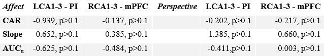
In the Experiment 1, participants were tasked with a gender categorization task, where they responded as accurately and quickly as possible to the gender of the voice they saw, while gender congruency (e.g., a male gesture paired with a male voice or a female gesture with a male voice) was manipulated. This manipulation served as direct control, enabling the investigation of automatic and implicit semantic interactions between gesture and speech. This relevant information was provided in the manuscript in Lines 167-172:‘An irrelevant factor of gender congruency (e.g., a man making a gesture combined with a female voice) was created[22,23,35]. This involved aligning the gender of the voice with the corresponding gender of the gesture in either a congruent (e.g., male voice paired with a male gesture) or incongruent (e.g., male voice paired with a female gesture) manner. This approach served as a direct control mechanism, facilitating the investigation of the automatic and implicit semantic interplay between gesture and speech[35]’. Correlation analyses were conducted to examine the TMS disruption effects on gender congruency, comparing reaction times for gender-incongruent versus congruent trials. No significant correlations were found between TMS disruption effects on either the IFG (Cathodal-tDCS effect with MI: r = 0.102, p = 0.677; Anodal-tDCS effect with MI: r = 0.178, p = 0.466) or pMTG (Cathodal-tDCS effect with MI: r \= -0.201, p = 0.410; Anodal-tDCS effect with MI: r = -0.232, p = 0.338).
Moreover, correlations between the TMS disruption effect on semantic congruency and both gesture entropy, speech entropy, and mutual information (MI) were examined. P-values of 0.290, 0.725, and 0.049 were observed, respectively.
The absence of a TMS effect on gender congruency, coupled with the lack of significance when correlated with the other information matrices, highlights the robustness of the significant finding at p = 0.049.
(4) The distributions of entropy for gestures and speech are very unequal. Whilst entropy for gestures has high variability, (.12-4.3), that of speech is very low (ceiling effect?) with low variance. Can the authors comment on whether they think this might have affected their analyses or results in any way? For example, do they think this could be a problem when calculating MI, which integrates both measures? L130-131.'
Response 4: We sincerely thank the reviewer for raising this insightful question. The core premise of the current study is that brain activity is modulated by the degree of information provided. Accordingly, the 20 entropy values for gesture and speech represent a subset of the overall entropy distribution, with the degree of entropy correlating with a distributed pattern of neural activity, regardless of the scale of variation. This hypothesis aligns with previous studies suggesting that neuronal activity is linked to the probability density of sensory information, with higher levels of uncertainty resulting in the engagement of a broader population of neurons, thereby reflecting the brain’s adaptive capacity to handle diverse possible interpretations (Fischer & Pena, 2011; Ganguli & Simoncelli, 2014).
Importantly, we conducted another EEG experiment with 30 subjects. Given the inherent differences between gesture and speech, it is important to note that speech, being more structurally distinct, tends to exhibit lower variability than gesture. To prevent an imbalance in the distribution of gesture and speech, we manipulated the information content of each modality. Specifically, we created three conditions for both gesture and speech (i.e., 0.75, 1, and 1.25 times the identification threshold), thereby ensuring comparable variance between the two modalities: gesture (mean entropy = 2.91 ± 1.01) and speech (mean entropy = 1.82 ± 0.71) (Author response table 6).
Full-factorial RSA analysis revealed an early P1 effect (0-100 ms) for gesture and a late LPC effect (734-780 ms) for speech (Author response image 2b). Crucially, the identified clusters showed significant correlations with both gesture (Author response image 2c1) and speech entropy (Author response image 2c3), respectively. These findings replicate the results of the present study, demonstrating that, irrespective of the variance in gesture and speech entropy, both modalities elicited ERP amplitude responses in a progressive manner that aligned with their respective information distributions.
Regarding the influence on MI values, since MI was calculated based on the overlapping responses between gesture and speech, a reduction in uncertainty during speech comprehension would naturally result in a smaller contribution to the MI value. However, as hypothesized above, the MI values were also assumed to represent a subset of the overall distribution, where the contributions of both gesture and speech are expected to follow a normal distribution. This hypothesis was further supported by our replication experiment. When the contributions of gesture and speech were balanced, a correlation between MI values and N400 amplitude was observed (Author response image 2c2), consistent with the results reported in the present manuscript. These findings not only support the idea that the correlation between MI and ERP components is unaffected by the subset of MI values but also confirm the replicability of our results.
Author response table 6.
Quantitative entropy for each gesture stimulus (BD: before discrimination point; DP: discrimination point; AD: after discrimination point) and speech stimulus (BI: before identification point; IP: identification point; AI: after identification point).
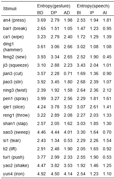
Author response image 2.
Results of group-level analysis and full-factorial RSA. a: The full-factorial representational similarity analysis (RSA) framework is illustrated schematically. Within the general linear model (GLM), the light green matrix denotes the representational dissimilarity matrix (RDM) for gesture semantic states, while light blue matrix represents speech semantic states, and the light red matrix illustrates the semantic congruency effect. The symbol ‘e’ indicates the random error term. All matrices, including the neural dissimilarity matrix, are structured as 18 * 18 matrices, corresponding to 18 conditions (comprising 3 gesture semantic states, 3 speech semantic states, and 2 congruency conditions). b: Coding strength for gesture states, speech states and congruency effect. Shaded clusters represent regions where each factor exhibited significant effects. Clusters with lower opacity correspond to areas where the grand-mean ERP amplitudes across conditions showed the highest correlation with unimodal entropy or MI. c1-c6: Topographical correlation maps illustrate the four significant RSA clusters (top), accompanied by the highest correlations between ERP amplitudes within the significant RSA clusters and the information matrices (bottom). Black dots represent electrodes exhibiting significant correlations, while black stars highlight the electrode with the highest correlation coefficient.
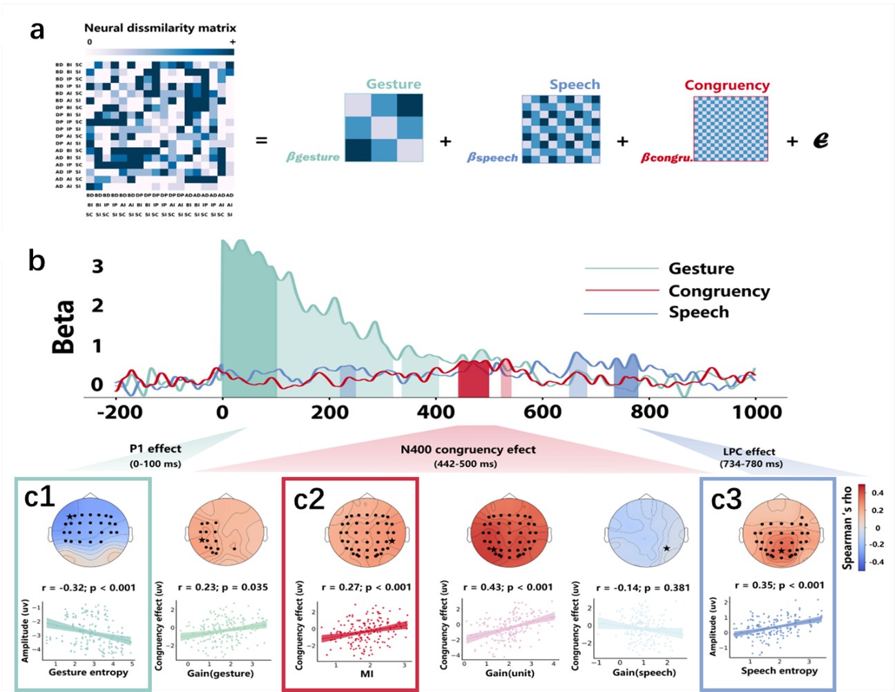
(5) L383: Why are the authors calling TW2 pre-lexical and TW6 post-lexical? I believe they must provide evidence or references justifying calling these periods pre- and post-lexical. This seems critical given the argument they're trying to make in this paragraph.
Response 5: The time windows (TWs) selected for the current study were based on our previous work (Zhao et al., 2021, J. Neurosci). In that study, we employed a double-pulse TMS protocol, delivering stimulation across eight 40-ms time windows: three windows preceding the speech identification point (TWs 1-3) and five windows following it (TWs 4-8). The pre-lexical time windows (TWs 1-3) occur before speech identification, while the post-lexical time windows (TWs 4-8) occur after this point. in the revised manuscript, we have made that clear in Lines 462-466:
“In TW2 of gesture-speech integration, which precedes the speech identification point23 and represents a pre-lexical stage, the suppression effect observed in the pMTG was correlated with speech entropy. Conversely, during TW6, which follows the speech identification point23 and represents a post-lexical stage, the IFG interruption effect was influenced by both gesture entropy, speech entropy, and their MI”
Reference:
Zhao, W., Li, Y., and Du, Y. (2021). TMS reveals dynamic interaction between inferior frontal gyrus and posterior middle temporal gyrus in gesture-speech semantic integration. The Journal of Neuroscience, 10356-10364. 10.1523/jneurosci.1355-21.2021.
(6) Below, I recommend the authors improve their description of the criteria employed to select ROIs. This is important for several reasons. For example, the lack of a control ROI presumably not implicated in integration makes the interpretation of the specificity of the results difficult. Additionally, other regions have been proposed more consistently by recent evidence as multimodal integrators, like for example, the angular gyrus (Humphreys, 2021), or the anterior temporal lobe. The inclusion of IFG as a key region for integration and the oversight of angular gyrus seems to me unjustified in the light of recent evidence.
Response 6: We appreciate the reviewer’s thoughtful consideration. The selection of IFG and pMTG as ROIs was based on a meta-analysis of multiple fMRI studies on gesture-speech integration, in which these two locations were consistently identified as activated. See Table 2 for details of the studies and coordinates of brain locations reported.
Author response table 7.
Meta-analysis of previous studies on gesture-speech integration.
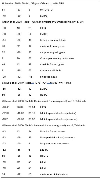
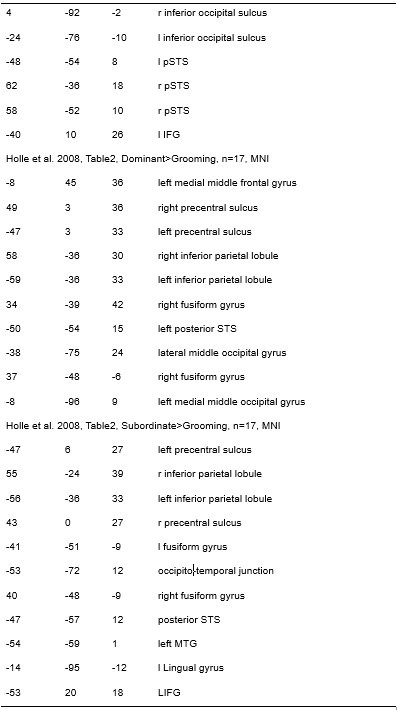
Based on the meta-analysis of previous studies, we selected the IFG and pMTG as ROIs for gesture-speech integration. The rationale for selecting these brain regions is outlined in the introduction in Lines 65-68: ‘Empirical studies have investigated the semantic integration between gesture and speech by manipulating their semantic relationship[15-18] and revealed a mutual interaction between them[19-21] as reflected by the N400 latency and amplitude[14] as well as common neural underpinnings in the left inferior frontal gyrus (IFG) and posterior middle temporal gyrus (pMTG)[15,22,23]’.
And further described in Lines 79-80: ‘_Experiment 1 employed high-definition transcranial direct current stimulation (HD-tDCS) to administer Anodal, Cathodal and Sham stimulation to either the IFG or the pMTG ’._ And Lines 87-90: ‘Given the differential involvement of the IFG and pMTG in gesture-speech integration, shaped by top-down gesture predictions and bottom-up speech processing [23], Experiment 2 was designed to assess whether the activity of these regions was associated with relevant informational matrices’.
In the Methods section, we clarified the selection of coordinates in Lines 193-199: ‘Building on a meta-analysis of prior fMRI studies examining gesture-speech integration[22], we targeted Montreal Neurological Institute (MNI) coordinates for the left IFG at (-62, 16, 22) and the pMTG at (-50, -56, 10). In the stimulation protocol for HD-tDCS, the IFG was targeted using electrode F7 as the optimal cortical projection site[36], with four return electrodes placed at AF7, FC5, F9, and FT9. For the pMTG, TP7 was selected as the cortical projection site36, with return electrodes positioned at C5, P5, T9, and P9.’
The selection of IFG or pMTG as integration hubs for gesture and speech has also been validated in our previous studies. Specifically, Zhao et al. (2018, J. Neurosci) applied TMS to both areas. Results demonstrated that disrupting neural activity in the IFG or pMTG via TMS selectively impaired the semantic congruency effect (reaction time costs due to semantic incongruence), while leaving the gender congruency effect unaffected. These findings identified the IFG and pMTG as crucial hubs for gesture-speech integration, guiding the selection of brain regions for our subsequent studies.
In addition, Zhao et al. (2021, J. Neurosci) employed a double-pulse TMS protocol across eight 40-ms time windows to explore the temporal dynamics of the IFG and pMTG. The results revealed time-window-selective disruptions of the semantic congruency effect, further supporting the dynamic and temporally staged involvement of these regions in gesture-speech integration.
While we have solid rationale for selecting the IFG and pMTG as key regions, we acknowledge the reviewer's point that the involvement of additional functionally and anatomically brain areas, cannot be excluded. We have included in the discussion as limitations in Lines 552-557: ‘Additionally, not all influenced TWs exhibited significant associations with entropy and MI. While HD-tDCS and TMS may impact functionally and anatomically connected brain regions[55,56], whether the absence of influence in certain TWs can be attributed to compensation by other connected brain areas, such as angular gyrus[57] or anterior temporal lobe[58], warrants further investigation. Therefore, caution is needed when interpreting the causal relationship between inhibition effects of brain stimulation and information-theoretic metrics (entropy and MI).’
References:
Willems, R.M., Ozyurek, A., and Hagoort, P. (2009). Differential roles for left inferior frontal and superior temporal cortex in multimodal integration of action and language. Neuroimage 47, 1992-2004. 10.1016/j.neuroimage.2009.05.066.
Drijvers, L., Jensen, O., and Spaak, E. (2021). Rapid invisible frequency tagging reveals nonlinear integration of auditory and visual information. Human Brain Mapping 42, 1138-1152. 10.1002/hbm.25282.
Drijvers, L., and Ozyurek, A. (2018). Native language status of the listener modulates the neural integration of speech and iconic gestures in clear and adverse listening conditions. Brain and Language 177, 7-17. 10.1016/j.bandl.2018.01.003.
Drijvers, L., van der Plas, M., Ozyurek, A., and Jensen, O. (2019). Native and non-native listeners show similar yet distinct oscillatory dynamics when using gestures to access speech in noise. Neuroimage 194, 55-67. 10.1016/j.neuroimage.2019.03.032.
Holle, H., and Gunter, T.C. (2007). The role of iconic gestures in speech disambiguation: ERP evidence. J Cognitive Neurosci 19, 1175-1192. 10.1162/jocn.2007.19.7.1175.
Kita, S., and Ozyurek, A. (2003). What does cross-linguistic variation in semantic coordination of speech and gesture reveal?: Evidence for an interface representation of spatial thinking and speaking. J Mem Lang 48, 16-32. 10.1016/S0749-596x(02)00505-3.
Bernardis, P., and Gentilucci, M. (2006). Speech and gesture share the same communication system. Neuropsychologia 44, 178-190. 10.1016/j.neuropsychologia.2005.05.007.
Zhao, W.Y., Riggs, K., Schindler, I., and Holle, H. (2018). Transcranial magnetic stimulation over left inferior frontal and posterior temporal cortex disrupts gesture-speech integration. Journal of Neuroscience 38, 1891-1900. 10.1523/Jneurosci.1748-17.2017.
Zhao, W., Li, Y., and Du, Y. (2021). TMS reveals dynamic interaction between inferior frontal gyrus and posterior middle temporal gyrus in gesture-speech semantic integration. The Journal of Neuroscience, 10356-10364. 10.1523/jneurosci.1355-21.2021.
Hartwigsen, G., Bzdok, D., Klein, M., Wawrzyniak, M., Stockert, A., Wrede, K., Classen, J., and Saur, D. (2017). Rapid short-term reorganization in the language network. Elife 6. 10.7554/eLife.25964.
Jackson, R.L., Hoffman, P., Pobric, G., and Ralph, M.A.L. (2016). The semantic network at work and rest: Differential connectivity of anterior temporal lobe subregions. Journal of Neuroscience 36, 1490-1501. 10.1523/JNEUROSCI.2999-15.2016.
Humphreys, G. F., Lambon Ralph, M. A., & Simons, J. S. (2021). A Unifying Account of Angular Gyrus Contributions to Episodic and Semantic Cognition. Trends in neurosciences, 44(6), 452–463. https://doi.org/10.1016/j.tins.2021.01.006
Bonner, M. F., & Price, A. R. (2013). Where is the anterior temporal lobe and what does it do?. The Journal of neuroscience : the official journal of the Society for Neuroscience, 33(10), 4213–4215. https://doi.org/10.1523/JNEUROSCI.0041-13.2013
(7) Some writing is obscure or unclear, in part due to superfluous words like 'intricate neural processes' on L74. Or the sentence in L47 - 48 about 'quantitatively functional mental states defined by a specific parser unified by statistical regularities' which, even read in context, fails to provide clarity about what a quantitatively functional mental state is, or how it is defined by specific parsers (or what these are), and what is the link to statistical regularities. In some cases, this lack of clarity leads to difficulties assessing the appropriateness of the methods, or the exact nature of the claims. For example, do they mean degree of comprehension instead of comprehensive value? I provide some more examples below:
Response 7: We appreciate the reviewer’s thoughtful consideration. The revised manuscript now includes a clear description and a detailed explanation of the association with the statistical logic, addressing the concerns raised in Lines 47-55: ‘Contemporary theories frame the semantic processing as a dynamic sequence of neural states[3], shaped by systems that are finely tuned to the statistical regularities inherent in sensory inputs[4]. These regularities enable the brain to evaluate, weight, and integrate multisensory information, optimizing the reliability of individual sensory signals [5]. However, sensory inputs available to the brain are often incomplete and uncertain, necessitating adaptive neural adjustments to resolve these ambiguities[6]. In this context, neuronal activity is thought to be linked to the probability density of sensory information, with higher levels of uncertainty resulting in the engagement of a broader population of neurons, thereby reflecting the brain’s adaptive capacity to handle diverse possible interpretations[7,8].’
References:
Brennan, J.R., Stabler, E.P., Van Wagenen, S.E., Luh, W.M., and Hale, J.T. (2016). Abstract linguistic structure correlates with temporal activity during naturalistic comprehension. Brain and Language 157, 81-94. 10.1016/j.bandl.2016.04.008.
Benetti, S., Ferrari, A., and Pavani, F. (2023). Multimodal processing in face-to-face interactions: A bridging link between psycholinguistics and sensory neuroscience. Front Hum Neurosci 17, 1108354. 10.3389/fnhum.2023.1108354.
Noppeney, U. (2021). Perceptual Inference, Learning, and Attention in a Multisensory World. Annual Review of Neuroscience, Vol 44, 2021 44, 449-473. 10.1146/annurev-neuro-100120-085519.
Ma, W.J., and Jazayeri, M. (2014). Neural coding of uncertainty and probability. Annu Rev Neurosci 37, 205-220. 10.1146/annurev-neuro-071013-014017.
Fischer, B.J., and Pena, J.L. (2011). Owl's behavior and neural representation predicted by Bayesian inference. Nat Neurosci 14, 1061-1066. 10.1038/nn.2872.
Ganguli, D., and Simoncelli, E.P. (2014). Efficient sensory encoding and Bayesian inference with heterogeneous neural populations. Neural Comput 26, 2103-2134. 10.1162/NECO_a_00638.
Comment 7.1: a) I am not too sure what they mean by 'response consistently provided by participants for four to six consecutive instances' [L117-118]. They should be clearer with the description of these 'pre-test' study methods.
Response 7.1: Thank you for this insightful question. An example of a participant's response to the gesture 'an' is provided below (Table 3). Initially, within 240 ms, the participant provided the answer "an," which could potentially be a guess. To ensure that the participant truly comprehends the gesture, we repeatedly present it until the participant’s response stabilizes, meaning the same answer is given consistently over several trials. While one might consider fixing the number of repetitions (e.g., six trials), this could lead to participants predicting the rule and providing the same answer out of habit. To mitigate this potential bias, we allow the number of repetitions to vary flexibly between four and six trials.
We understand that the initial phrase might be ambiguous, in the revised manuscript, we have changed the phrase into: ‘For each gesture or speech, the action verb consistently provided by participants across four to six consecutive repetitions—with the number of repetitions varied to mitigate learning effects—was considered the comprehensive response for the gesture or speech.’ (Lines 130-133)
Author response table 8.
Example of participant's response to the gesture 'an'
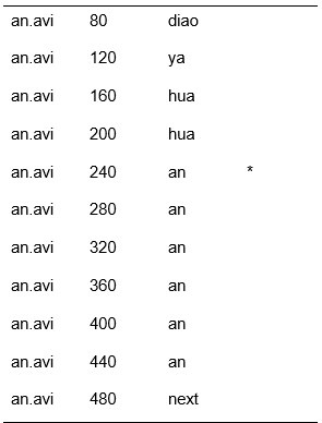
Comment 7.2: b) I do not understand the paragraph in L143 - 146. This is important to rephrase for clarification. What are 'stepped' neural changes? What is the purpose of 'aggregating' neural responses with identical entropy / MI values?
Response 7.2: It is important to note that the 20 stimuli exhibit 20 increments of gesture entropy values, 11 increments of speech entropy values, and 19 increments of mutual information values (Appendix Table 3). This discrepancy arises from the calculation of entropy and mutual information, where the distributions were derived from the comprehensive set of responses contributed by all 30 participants. As a result, these values were impacted not only by the distinct nameabilities of the stimuli but also by the entirety of responses provided. Consequently, in the context of speech entropy, 9 items demonstrate the nameability of 1, signifying unanimous comprehension among all 30 participants, resulting in an entropy of 0. Moreover, stimuli 'ning' and 'jiao' share an identical distribution, leading to an entropy of 0.63. Regarding MI, a value of 0.66 is computed for the combinations of stimuli 'sao' (gesture entropy: 4.01, speech entropy: 1.12, Author response image 32) and 'tui' (gesture entropy: 1.62, speech entropy: 0, Author response image 4). This indicates that these two sets of stimuli manifest an equivalent degree of integration.
Author response image 3.
Example of gesture answers (gesture sao), speech answers (speech sao), and mutual information (MI) for the ‘sao’ item
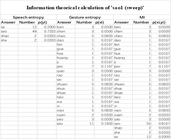
Author response image 4.
Example of gesture answers (gesture tui), speech answers (speech tui), and mutual information (MI) for the ‘tui’ item
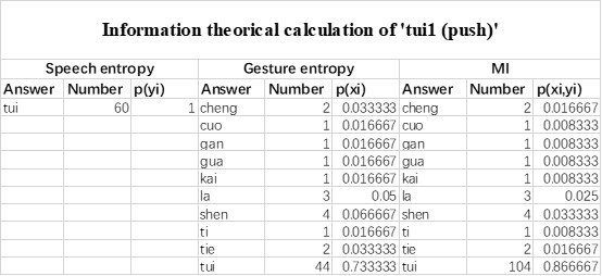
To precisely assess whether lower entropy/MI corresponds to a smaller or larger neural response, neural responses (ERP amplitude or TMS inhibition effect) with identical entropy or MI values were averaged before undergoing correlational analysis. We understand that the phrasing might be ambiguous. Clear description has been changed in the revised manuscript in Lines 157-160: ‘To determine whether entropy or MI values corresponds to distinct neural changes, the current study first aggregated neural responses (including inhibition effects of tDCS and TMS or ERP amplitudes) that shared identical entropy or MI values, prior to conducting correlational analyses.’
Comment 7.3: c) The paragraph in L160-171 is confusing. Is it an attempt to give an overview of all three experiments? If so, consider moving to the end or summarising what each experiment is at the beginning of the paragraph giving it a name (i.e., TMS). Without that, it is unclear what each experiment is counterbalancing or what 'stimulation site' refers to, for example, leading to a significant lack of clarity.
Response 7.3: We are sorry for the ambiguity, in the revised manuscript, we have moved the relevant phrasing to the beginning of each experiment.
‘Experiment 1: HD-tDCS protocol and data analysis
Participants were divided into two groups, with each group undergoing HD-tDCS stimulation at different target sites (IFG or pMTG). Each participant completed three experimental sessions, spaced one week apart, during which 480 gesture-speech pairs were presented across various conditions. In each session, participants received one of three types of HD-tDCS stimulation: Anodal, Cathodal, or Sham. The order of stimulation site and type was counterbalanced using a Latin square design to control for potential order effects’ (Lines 183-189)
‘Experiment 2: TMS protocol and data analysis
Experiment 2 involved 800 gesture-speech pairs, presented across 15 blocks over three days, with one week between sessions. Stimulation was administered at three different sites (IFG, pMTG, or Vertex). Within the time windows (TWs) spanning the gesture-speech integration period, five TWs that exhibited selective disruption of integration were selected: TW1 (-120 to -80 ms relative to the speech identification point), TW2 (-80 to -40 ms), TW3 (-40 to 0 ms), TW6 (80 to 120 ms), and TW7 (120 to 160 ms)23 (Figure 1C). The order of stimulation site and TW was counterbalanced using a Latin square design.’ (Lines 223-230)
‘Experiment 3: Electroencephalogram (EEG) recording and data analysis
Experiment 3, comprising a total of 1760 gesture-speech pairs, was completed in a single-day session.’ (Lines 249-250)
Comment 7.4: d) L402-406: This sentence is not clear. What do the authors mean by 'the state of [the neural landscape] constructs gradually as measured by entropy and MI'? How does this construct a neural landscape? The authors must rephrase this paragraph using clearer language since in its current state it is very difficult to assess whether it is supported by the evidence they present.
Response 7.4: We are sorry for the ambiguity, in the revised manuscript we have provided clear description in Lines 483-492: ‘The varying contributions of unisensory gesture-speech information and the convergence of multisensory inputs, as reflected in the correlation between distinct ERP components and TMS time windows (TMS TWs), are consistent with recent models suggesting that multisensory processing involves parallel detection of modality-specific information and hierarchical integration across multiple neural levels[4,48]. These processes are further characterized by coordination across multiple temporal scales[49]. Building on this, the present study offers additional evidence that the multi-level nature of gesture-speech processing is statistically structured, as measured by information matrix of unisensory entropy and multisensory convergence index of MI, the input of either source would activate a distributed representation, resulting in progressively functioning neural responses’
References:
Benetti, S., Ferrari, A., and Pavani, F. (2023). Multimodal processing in face-to-face interactions: A bridging link between psycholinguistics and sensory neuroscience. Front Hum Neurosci 17, 1108354. 10.3389/fnhum.2023.1108354.
Meijer, G.T., Mertens, P.E.C., Pennartz, C.M.A., Olcese, U., and Lansink, C.S. (2019). The circuit architecture of cortical multisensory processing: Distinct functions jointly operating within a common anatomical network. Prog Neurobiol 174, 1-15. 10.1016/j.pneurobio.2019.01.004.
Senkowski, D., and Engel, A.K. (2024). Multi-timescale neural dynamics for multisensory integration. Nat Rev Neurosci 25, 625-642. 10.1038/s41583-024-00845-7.
(8) Some writing suffers from conceptual equivocation. For example, the link between 'multimodal representation' and gesture as a type of multimodal extralinguistic information is not straightforward. What 'multimodal representations' usually refer to in semantic cognition is not the co-occurrence of gesture and speech, but the different sources or modalities that inform the structure of a semantic representation or concept (not the fact we use another modality vision to perceive gestures that enrich the linguistic auditory communication of said concepts). See also my comment in the public review regarding the conceptual conflation of the graded hub hypothesis.
Response 8: We aimed to clarify that the integration of gesture and speech, along with the unified representation it entails, is not merely a process whereby perceived gestures enhance speech comprehension. Rather, there exists a bidirectional influence between these two modalities, affecting both their external forms (Bernaidis et al., 2006) and their semantic content (Kita et al., 2003; Kelly et al., 2010). Given that multisensory processing is recognized as an interplay of both top-down and bottom-up mechanisms, we hypothesize that this bidirectional semantic influence between gesture and speech operates similarly. Consequently, we recorded neural responses—specifically the inhibitory effects observed through TMS/tDCS or ERP components—beginning at the onset of speech, which marks the moment when both modalities are accessible.
We prioritize gesture for two primary reasons. Firstly, from a naturalistic perspective, speech and gesture are temporally aligned; gestures typically precede their corresponding speech segments by less than one second (Morrelsamuls et al., 1992). This temporal alignment has prompted extensive research aimed at identifying the time windows during which integration occurs (Obermeier et al., 2011, 2015). Results indicate that local integration of gesture and speech occurs within a time frame extending from -200 ms to +120 ms relative to gesture-speech alignment, where -200 ms indicates that gestures occur 200 ms before speech onset, and +120 ms signifies gestures occurring after the identification point of speech.
Secondly, in our previous study (Zhao, 2023), we investigated this phenomenon by manipulating gesture-speech alignment across two conditions: (1) gestures preceding speech by a fixed interval of 200 ms, and (2) gestures preceding speech at its semantic identification point. Notably, only in the second condition did we observe time-window-selective disruptions of the semantic congruency effect in the IFG and pMTG. This led us to conclude that gestures serve a semantic priming function for co-occurring speech.
We recognize that our previous use of the term "co-occurring speech" may have led to ambiguity. Therefore, in the revised manuscript, we have replaced those sentences with a detailed description of the properties of each modality in Lines 60-62: ‘Even though gestures convey information in a global-synthetic way, while speech conveys information in a linear segmented way, there exists a bidirectional semantic influence between the two modalities[9,10]’
Conceptual conflation of the graded hub hypothesis has been clarified in the Response to Reviewer 3 (public review) response 2.
References:
Bernardis, P., & Gentilucci, M. (2006). Speech and gesture share the same communication system. Neuropsychologia, 44(2), 178-190
Kelly, S. D., Ozyurek, A., & Maris, E. (2010b). Two sides of the same coin: speech and gesture mutually interact to enhance comprehension. Psychological Science, 21(2), 260-267. doi:10.1177/0956797609357327
Kita, S., & Ozyurek, A. (2003). What does cross-linguistic variation in semantic coordination of speech and gesture reveal?: Evidence for an interface representation of spatial thinking and speaking. Journal of Memory and Language, 48(1), 16-32. doi:10.1016/s0749-596x(02)00505-3
Obermeier, C., & Gunter, T. C. (2015). Multisensory Integration: The Case of a Time Window of Gesture-Speech Integration. Journal of Cognitive Neuroscience, 27(2), 292-307. doi:10.1162/jocn_a_00688
Obermeier, C., Holle, H., & Gunter, T. C. (2011). What Iconic Gesture Fragments Reveal about Gesture-Speech Integration: When Synchrony Is Lost, Memory Can Help. Journal of Cognitive Neuroscience, 23(7), 1648-1663. doi:10.1162/jocn.2010.21498
Morrelsamuels, P., & Krauss, R. M. (1992). WORD FAMILIARITY PREDICTS TEMPORAL ASYNCHRONY OF HAND GESTURES AND SPEECH. Journal of Experimental Psychology-Learning Memory and Cognition, 18(3), 615-622. doi:10.1037/0278-7393.18.3.615
Hostetter, A., and Mainela-Arnold, E. (2015). Gestures occur with spatial and Motoric knowledge: It's more than just coincidence. Perspectives on Language Learning and Education 22, 42-49. doi:10.1044/lle22.2.42.
McNeill, D. (2005). Gesture and though (University of Chicago Press). 10.7208/chicago/9780226514642.001.0001.
Zhao, W. (2023). TMS reveals a two-stage priming circuit of gesture-speech integration. Front Psychol 14, 1156087. 10.3389/fpsyg.2023.1156087.
(9) The last paragraph of the introduction lacks a conductive thread. The authors describe three experiments without guiding the reader through a connecting thread underlying the experiments. Feels more like three disconnected studies than a targeted multi-experiment approach to solve a problem. What is each experiment contributing to? What is the 'grand question' or thread unifying these?
Response 9: The present study introduced three experiments to explore the neural activity linked to the amount of information processed during multisensory gesture-speech integration. In Experiment 1, we observed that the extent of inhibition in the pMTG and LIFG was closely linked to the overlapping gesture-speech responses, as quantified by mutual information. Building on the established roles of the pMTG and LIFG in our previous study (Zhao et al., 2021, JN), we then expanded our investigation to determine whether the dynamic neural engagement between the pMTG and LIFG during gesture-speech processing was also associated with the quality of the information. This hypothesis was further validated through high-temporal resolution EEG, where we examined ERP components related to varying information qualities. Notably, we observed a close time alignment between the ERP components and the time windows of the TMS effects, which were associated with the same informational matrices in gesture-speech processing.
Linkage of the three experiments has been clarified in the introduction in Lines 75-102: ‘
To investigate the neural mechanisms underlying gesture-speech integration, we conducted three experiments to assess how neural activity correlates with distributed multisensory integration, quantified using information-theoretic measures of MI. Additionally, we examined the contributions of unisensory signals in this process, quantified through unisensory entropy. Experiment 1 employed high-definition transcranial direct current stimulation (HD-tDCS) to administer Anodal, Cathodal and Sham stimulation to either the IFG or the pMTG. HD-tDCS induces membrane depolarization with anodal stimulation and membrane hyperpolarization with cathodal stimulation[26], thereby increasing or decreasing cortical excitability in the targeted brain area, respectively. This experiment aimed to determine whether the overall facilitation (Anodal-tDCS minus Sham-tDCS) and/or inhibitory (Cathodal-tDCS minus Sham-tDCS) of these integration hubs is modulated by the degree of gesture-speech integration, as measure by MI.
Given the differential involvement of the IFG and pMTG in gesture-speech integration, shaped by top-down gesture predictions and bottom-up speech processing [23], Experiment 2 was designed to further assess whether the activity of these regions was associated with relevant informational matrices. Specifically, we applied inhibitory chronometric double-pulse transcranial magnetic stimulation (TMS) to specific temporal windows associated with integration processes in these regions[23], assessing whether the inhibitory effects of TMS were correlated with unisensory entropy or the multisensory convergence index (MI).
Experiment 3 complemented these investigations by focusing on the temporal dynamics of neural responses during semantic processing, leveraging high-temporal event-related potentials (ERPs). This experiment investigated how distinct information contributors modulated specific ERP components associated with semantic processing. These components included the early sensory effects as P1 and N1–P2[27,28], the N400 semantic conflict effect[14,28,29], and the late positive component (LPC) reconstruction effect[30,31]. By integrating these ERP findings with results from Experiments 1 and 2, Experiment 3 aimed to provide a more comprehensive understanding of how gesture-speech integration is modulated by neural dynamics’
References:
Bikson, M., Inoue, M., Akiyama, H., Deans, J.K., Fox, J.E., Miyakawa, H., and Jefferys, J.G.R. (2004). Effects of uniform extracellular DC electric fields on excitability in rat hippocampal slices. J Physiol-London 557, 175-190. 10.1113/jphysiol.2003.055772.
Federmeier, K.D., Mai, H., and Kutas, M. (2005). Both sides get the point: hemispheric sensitivities to sentential constraint. Memory & Cognition 33, 871-886. 10.3758/bf03193082.
Kelly, S.D., Kravitz, C., and Hopkins, M. (2004). Neural correlates of bimodal speech and gesture comprehension. Brain and Language 89, 253-260. 10.1016/s0093-934x(03)00335-3.
Wu, Y.C., and Coulson, S. (2005). Meaningful gestures: Electrophysiological indices of iconic gesture comprehension. Psychophysiology 42, 654-667. 10.1111/j.1469-8986.2005.00356.x.
Fritz, I., Kita, S., Littlemore, J., and Krott, A. (2021). Multimodal language processing: How preceding discourse constrains gesture interpretation and affects gesture integration when gestures do not synchronise with semantic affiliates. J Mem Lang 117, 104191. 10.1016/j.jml.2020.104191.
Gunter, T.C., and Weinbrenner, J.E.D. (2017). When to take a gesture seriously: On how we use and prioritize communicative cues. J Cognitive Neurosci 29, 1355-1367. 10.1162/jocn_a_01125.
Ozyurek, A., Willems, R.M., Kita, S., and Hagoort, P. (2007). On-line integration of semantic information from speech and gesture: Insights from event-related brain potentials. J Cognitive Neurosci 19, 605-616. 10.1162/jocn.2007.19.4.605.
Zhao, W., Li, Y., and Du, Y. (2021). TMS reveals dynamic interaction between inferior frontal gyrus and posterior middle temporal gyrus in gesture-speech semantic integration. The Journal of Neuroscience, 10356-10364. 10.1523/jneurosci.1355-21.2021.
(10) The authors should provide a clearer figure to appreciate their paradigm, illustrating clearly the stimulus presentation (gesture and speech).
Response 10: To reduce ambiguity, unnecessary arrows were deleted from Figure 1.
Comment 11.1: (11) Required methodological clarifications to better assess the strength of the evidence presented:
a) Were the exclusion criteria only handedness and vision? Did the authors exclude based on neurological and psychiatric disorders? Psychoactive drugs? If not, do they think the lack of these exclusion criteria might have influenced their results?
Response 11.1: Upon registration, each participant is required to complete a questionnaire alongside the consent form and handedness questionnaire. This procedure is designed to exclude individuals with potential neurological or psychiatric disorders, as well as other factors that may affect their mental state or reaction times. Consequently, all participants reported in the manuscript do not have any of the aforementioned neurological or psychiatric disorders. The questionnaire is attached below:
Author response image 4.
Comment 11.2: b) Are the subjects from the pre-tests (L112-113) and the replication study (L107) a separate sample or did they take part in Experiments 1-3?
Response 11.2: The participants in each pre-test and experiment were independent, resulting in a total of 188 subjects. Since the stimuli utilized in this study were previously validated and reported (Zhao et al., 2021), the 90 subjects who participated in the three pre-tests are not included in the final count for the current study, leaving a total of 98 participants reported in the manuscript in Lines 103-104: ‘Ninety-eight young Chinese participants signed written informed consent forms and took part in the present study’.
Comment 11.3: c) L176. The authors should explain how they selected ROIs. This is very important for the reasons outlined above.
Response 11.3: Please see Response to Comment 6 for details.
Comment 11.4: d) The rationale for Experiment 1 and its analysis approach should be explicitly described. Why perform Pearson correlations? What is the conceptual explanation of the semantic congruency effect and why should it be expected to correlate with the three information-theoretic metrics? What effects could the authors expect to find and what would they mean? There is a brief description in L187-195 but it is unclear.
Response 11.4: We thank the reviewer for their rigorous consideration. The semantic congruency effect is widely used as an index of multisensory integration. Therefore, the effects of HD-tDCS on the IFG and pMTG, as measured by changes in the semantic congruency effect, serve as an indicator of altered neural responses to multisensory integration. In correlating these changes with behavioral indices of information degree, we aimed to assess whether the integration hubs (IFG and pMTG) function progressively during multisensory gesture-speech integration. The rationale for using Pearson correlations is based on the hypothesis that the 20 sets of stimuli used in this study represent a sample from a normally distributed population. Thus, even with changes in the sample (e.g., using another 20 values), the gradual relationship between neural responses and the degree of information would remain unchanged. This hypothesis is supported by the findings from another experiment (see details in Response to Comment 4).
In the revised manuscript, we have provided a clear description of the rationale for Experiment 1 in Lines 206-219: ‘To examine the relationship between the degree of information and neural responses, we conducted Pearson correlation analyses using a sample of 20 sets. Neural responses were quantified based on the effects of HD-tDCS (active tDCS minus sham tDCS) on the semantic congruency effect, defined as the difference in reaction times between semantic incongruent and congruent conditions (Rt(incongruent) - Rt(congruent)). This effect served as an index of multisensory integration[35] within the left IFG and pMTG. The variation in information was assessed using three information-theoretic metrics. To account for potential confounds related to multiple candidate representations, we conducted partial correlation analyses between the tDCS effects and gesture entropy, speech entropy, and MI, controlling for the number of responses provided for each gesture and speech, as well as the total number of combined responses. Given that HD-tDCS induces overall disruption at the targeted brain regions, we hypothesized that the neural activity within the left IFG and pMTG would be progressively affected by varying levels of multisensory convergence, as indexed by MI.’
Additionally, in the introduction, we have rephrased the relevant rationale in Lines 75-86: _‘_To investigate the neural mechanisms underlying gesture-speech integration, we conducted three experiments to assess how neural activity correlates with distributed multisensory integration, quantified using information-theoretic measures of MI. Additionally, we examined the contributions of unisensory signals in this process, quantified through unisensory entropy. Experiment 1 employed high-definition transcranial direct current stimulation (HD-tDCS) to administer Anodal, Cathodal and Sham stimulation to either the IFG or the pMTG. HD-tDCS induces membrane depolarization with anodal stimulation and membrane hyperpolarization with cathodal stimulation[26], thereby increasing or decreasing cortical excitability in the targeted brain area, respectively. This experiment aimed to determine whether the overall facilitation (Anodal-tDCS minus Sham-tDCS) and/or inhibitory (Cathodal-tDCS minus Sham-tDCS) of these integration hubs is modulated by the degree of gesture-speech integration, as measure by MI
Reference:
Kelly, S.D., Creigh, P., and Bartolotti, J. (2010). Integrating speech and iconic gestures in a Stroop-like task: Evidence for automatic processing. Journal of Cognitive Neuroscience 22, 683-694. 10.1162/jocn.2009.21254.
Comment 11.5: e) The authors do not mention in the methods if FDR correction was applied to the Pearson correlations in Experiment 1. There is a mention in the Results Figure, but it is unclear if it was applied consistently. Can the authors confirm, and explicitly state the way they carried out FDR correction for this family of tests in Experiment 1? This is especially important in the light of some of their results having a p-value of p=.049.
Response 11.5: FDR correction was applied to Experiment 1, and all reported p-values were corrected using this method. In the revised manuscript, we have included a reference to FDR correction in Lines 221-222: ‘False discovery rate (FDR) correction was applied for multiple comparisons.’
In Experiment 1, since two separate participant groups (each N = 26) were recruited for the HD-tDCS over either the IFG or pMTG, FDR correction was performed separately for each group. Therefore, for each brain region, six comparisons (three information matrices × two tDCS effects: anodal-sham or cathodal-sham) were submitted for FDR correction.
In Experiment 2, six comparisons (three information matrices × two sites: IFG or pMTG) were submitted for FDR correction. In Experiment 3, FDR correction was applied to the seven regions of interest (ROIs) within each component, resulting in five comparisons
The confidence of a p-value of 0.049 was clarified in Response to Comment 3.
Comment 11.6: f) L200. What does the abbreviation 'TW' stands for in this paragraph? When was it introduced in the main text? The description is in the Figure, but it should be moved to the main text.]
Comment 11.7: g) How were the TWs chosen? Is it the criterion in L201-203? If so, it should be moved to the start of the paragraph. What does the word 'selected' refer to in that description? Selected for what? The explanation seems to be in the Figure, but it should be in the main text. It is still not a complete explanation. What were the criteria for assigning TWs to the IFG or pMTG?
Response 11.6& 11.7: Since the two comments are related, we will provide a synthesized response. 'TW' refers to time window, the selection of which was based on our previous study (Zhao et al., 2021, J. Neurosci). In Zhao et al. (2021), we employed the same experimental protocol—using inhibitory double-pulse transcranial magnetic stimulation (TMS) over the IFG and pMTG in one of eight 40-ms time windows relative to the speech identification point (IP; the minimal length of lexical speech), with three time windows before the speech IP and five after. Based on this previous work, we believe that these time windows encompass the potential gesture-speech integration process. Results demonstrated a time-window-selective disruption of the semantic congruency effect (i.e., reaction time costs driven by semantic conflict), with no significant modulation of the gender congruency effect (i.e., reaction time costs due to gender conflict), when stimulating the left pMTG in TW1, TW2, and TW7, and when stimulating the left IFG in TW3 and TW6. Based on these findings, the present study selected the five time windows that showed a selective disruption effect during gesture-speech integration.
Note that in the present study, we applied stimulation to both the IFG and pMTG across all five time windows, and further correlated the TMS disruption effects with the three information matrices.
We recognize that the rationale for the choice of time windows was not sufficiently explained in the original manuscript. In the revised manuscript, we have added the relevant description in Lines 223-228: ‘Stimulation was administered at three different sites (IFG, pMTG, or Vertex). Within the time windows (TWs) spanning the gesture-speech integration period, five TWs that exhibited selective disruption of integration were selected: TW1 (-120 to -80 ms relative to the speech identification point), TW2 (-80 to -40 ms), TW3 (-40 to 0 ms), TW6 (80 to 120 ms), and TW7 (120 to 160 ms)[23] (Figure 1C). The order of stimulation site and TW was counterbalanced using a Latin square design.’
Comment 11.8: h) Again, the rationale for the Pearson correlations of semantic congruency with information-theoretic metrics should be explicitly outlined. What is this conceptually?
Response 11.8: Given that the rationale behind Experiment 1 and Experiment 2 is similar—both investigating the correlation between interrupted neural effects and the degree of information—we believe that the introduction of the Pearson correlation between semantic congruency and information-theoretic metrics, as presented in Experiment 1 (see Response to Comment 11.4 for details), is sufficient for both experiments.
Comment 11.9: i)What does 'gesture stoke' mean in the Figure referring to Experiment 3? Figure 1D is not clear. What are the arrows referring to?
Response 11.9: According to McNeill (1992), gesture phases differ based on whether the gesture depicts imagery. Iconic and metaphoric gestures are imagistic and typically consist of three phases: a preparation phase, a stroke phase, and a retraction phrase. Figure 4 provides an example of these three phases using the gesture ‘break’. In the preparation phase, the hand and arm move away from their resting position to a location in gesture space where the stroke begins. As illustrated in the first row of Figure 4, during the preparation phase of the ‘break’ gesture, the hands, initially in a fist and positioned downward, rise to a center-front position. In the stroke phase, the meaning of the gesture is conveyed. This phase occurs in the central gesture space and is synchronized with the linguistic segments it co-expresses. For example, in the stroke phase of the ‘break’ gesture (second row of Figure 4), the two fists move 90 degrees outward before returning to a face-down position. The retraction phase involves the return of the hand from the stroke position to the rest position. In the case of the ‘break’ gesture, this involves moving the fists from the center front back into the resting position (see third row of Figure 4).
Therefore, in studies examining gesture-speech integration, gestures are typically analyzed starting from the stroke phase (Habets et al., 2011; Kelly et al., 2010), a convention also adopted in our previous studies (Zhao et al., 2018, 2021, 2023). We acknowledge that this should be explained explicitly, and in the revised manuscript, we have added the following clarification in Lines 162-166: ‘Given that gestures induce a semantic priming effect on concurrent speech[33], this study utilized a semantic priming paradigm in which speech onset was aligned with the DP of each gesture[23,33], the point at which the gesture transitions into a lexical form[34]. The gesture itself began at the stroke phase, a critical moment when the gesture conveys its primary semantic content[34].’
Additionally, Figure 1 has been revised in the manuscript to eliminate ambiguous arrows. (see Response 10 for detail).
Author response image 5.
An illustration of the gesture phases of the 'break' gesture.
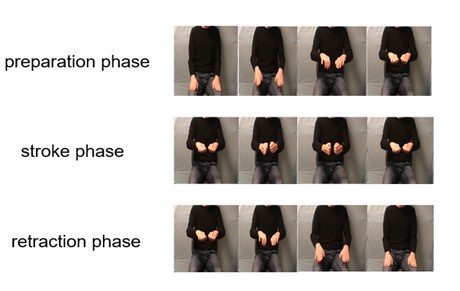
References:
Habets, B., Kita, S., Shao, Z. S., Ozyurek, A., & Hagoort, P. (2011). The Role of Synchrony and Ambiguity in Speech-Gesture Integration during Comprehension. Journal of Cognitive Neuroscience, 23(8), 1845-1854. doi:10.1162/jocn.2010.21462
Kelly, S. D., Creigh, P., & Bartolotti, J. (2010). Integrating Speech and Iconic Gestures in a Stroop-like Task: Evidence for Automatic Processing. Journal of Cognitive Neuroscience, 22(4), 683-694. doi:DOI 10.1162/jocn.2009.21254
Comment 11.10: j) L236-237: "Consequently, four ERP components were predetermined" is very confusing. Were these components predetermined? Or were they determined as a consequence of the comparison between the higher and lower halves for the IT metrics described above in the same paragraph? The description of the methods is not clear.
Response 11.10: The components selected were based on a comparison between the higher and lower halves of the information metrics. By stating that these components were predetermined, we aimed to emphasize that the components used in our study are consistent with those identified in previous research on semantic processing. We acknowledge that the phrasing may have been unclear, and in the revised manuscript, we have provided a more explicit description in Lines 267-276: ‘To consolidate the data, we conducted both a traditional region-of-interest (ROI) analysis, with ROIs defined based on a well-established work[40], and a cluster-based permutation approach, which utilizes data-driven permutations to enhance robustness and address multiple comparisons.
For the traditional ROI analysis, grand-average ERPs at electrode Cz were compared between the higher (≥50%) and lower (<50%) halves for gesture entropy (Figure 5A1), speech entropy (Figure 5B1), and MI (Figure 5C1). Consequently, four ERP components were determined: the P1 effect observed within the time window of 0-100 ms[27,28], the N1-P2 effect observed between 150-250ms[27,28], the N400 within the interval of 250-450ms[14,28,29], and the LPC spanning from 550-1000ms[30,31].’
Reference: Habets, B., Kita, S., Shao, Z.S., Ozyurek, A., and Hagoort, P. (2011). The Role of Synchrony and Ambiguity in Speech-Gesture Integration during Comprehension. J Cognitive Neurosci 23, 1845-1854. 10.1162/jocn.2010.21462.
(12) In the Results section for Experiment 2 (L292-295), it is not clear what the authors mean when they mention that a more negative TMS effect represents a stronger interruption of the integration effect. If I understand correctly, the correlation reported for pMTG was for speech entropy, which does not represent integration (that would be MI).
Response 12: Since the TMS effect was defined as active TMS minus Vertex TMS, the inhibitory TMS effect is inherently negative. A greater inhibitory TMS effect corresponds to a larger negative value, such that a more negative TMS effect indicates a stronger disruption of the integration process. We acknowledge that the previous phrasing was somewhat ambiguous. In the revised manuscript, we have rephrased the sentence as follows: ‘a larger negative TMS effect signifies a greater disruption of the integration process’ (Lines 342-343)
Multisensory integration transcends simple data amalgamation, encompassing complex interactions at various hierarchical neural levels and the parallel detection and discrimination of raw data from each modality (Benetti et al., 2023; Meijer et al., 2019). Therefore, we regard the process of gesture-speech integration as involving both unisensory processing and multisensory convergence. The correlation of gesture and speech entropy reflects contributions from unisensory processing, while the mutual information (MI) index indicates the contribution of multisensory convergence during gesture-speech integration. The distinction between these various source contributions will be the focus of Experiment 2 and Experiment 3, as described in the revised manuscript Lines 87-102: ‘Given the differential involvement of the IFG and pMTG in gesture-speech integration, shaped by top-down gesture predictions and bottom-up speech processing [23], Experiment 2 was designed to further assess whether the activity of these regions was associated with relevant informational matrices. Specifically, we applied inhibitory chronometric double-pulse transcranial magnetic stimulation (TMS) to specific temporal windows associated with integration processes in these regions[23], assessing whether the inhibitory effects of TMS were correlated with unisensory entropy or the multisensory convergence index (MI).
Experiment 3 complemented these investigations by focusing on the temporal dynamics of neural responses during semantic processing, leveraging high-temporal event-related potentials (ERPs). This experiment investigated how distinct information contributors modulated specific ERP components associated with semantic processing. These components included the early sensory effects as P1 and N1–P2[27,28], the N400 semantic conflict effect[14,28,29], and the late positive component (LPC) reconstruction effect[30,31]. By integrating these ERP findings with results from Experiments 1 and 2, Experiment 3 aimed to provide a more comprehensive understanding of how gesture-speech integration is modulated by neural dynamics’.
References:
Benetti, S., Ferrari, A., and Pavani, F. (2023). Multimodal processing in face-to-face interactions: A bridging link between psycholinguistics and sensory neuroscience. Front Hum Neurosci 17, 1108354. 10.3389/fnhum.2023.1108354.
Meijer, G.T., Mertens, P.E.C., Pennartz, C.M.A., Olcese, U., and Lansink, C.S. (2019). The circuit architecture of cortical multisensory processing: Distinct functions jointly operating within a common anatomical network. Prog Neurobiol 174, 1-15. 10.1016/j.pneurobio.2019.01.004.
(13) I find the description of the results for Experiment 3 very hard to follow. Perhaps if the authors have decided to organise the main text by describing the components from earliest to latest, the Figure organisation should follow suit (i.e., organise the Figure from the earliest to the latest component, instead of gesture entropy/speech entropy / mutual information). This might make the description of the results easier to follow.
Response 13: As suggested, we have reorganized the results of experiment 3 based on components from earliest to latest, together with an updated Figure 5.
The results are detailed in Lines 367-423: ‘Topographical maps illustrating amplitude differences between the lower and higher halves of speech entropy demonstrate a central-posterior P1 amplitude (0-100 ms, Figure 5B). Aligning with prior findings[27], the paired t-tests demonstrated a significantly larger P1 amplitude within the ML ROI (t(22) = 2.510, p = 0.020, 95% confidence interval (CI) = [1.66, 3.36]) when contrasting stimuli with higher 50% speech entropy against those with lower 50% speech entropy (Figure 5D1 left). Subsequent correlation analyses unveiled a significant increase in the P1 amplitude with the rise in speech entropy within the ML ROI (r = 0.609, p = 0.047, 95% CI = [0.039, 1.179], Figure 5D1 right). Furthermore, a cluster of neighboring time-electrode samples exhibited a significant contrast between the lower 50% and higher 50% of speech entropy, revealing a P1 effect spanning 16 to 78 ms at specific electrodes (FC2, FCz, C1, C2, Cz, and CPz, Figure 5D2 middle) (t(22) = 2.754, p = 0.004, 95% confidence interval (CI) = [1.65, 3.86], Figure 5D2 left), with a significant correlation with speech entropy (r = 0.636, p = 0.035, 95% CI = [0.081, 1.191], Figure 5D2 right).
Additionally, topographical maps comparing the lower 50% and higher 50% gesture entropy revealed a frontal N1-P2 amplitude (150-250 ms, Figure 5A). In accordance with previous findings on bilateral frontal N1-P2 amplitude[27], paired t-tests displayed a significantly larger amplitude for stimuli with lower 50% gesture entropy than with higher 50% entropy in both ROIs of LA (t(22) = 2.820, p = 0.011, 95% CI = [2.21, 3.43]) and RA (t(22) = 2.223, p = 0.038, 95% CI = [1.56, 2.89]) (Figure 5E1 left). Moreover, a negative correlation was found between N1-P2 amplitude and gesture entropy in both ROIs of LA (r = -0.465, p = 0.039, 95% CI = [-0.87, -0.06]) and RA (r = -0.465, p = 0.039, 95% CI = [-0.88, -0.05]) (Figure 5E1 right). Additionally, through a cluster-permutation test, the N1-P2 effect was identified between 184 to 202 ms at electrodes FC4, FC6, C2, C4, C6, and CP4 (Figure 5E2 middle) (t(22) = 2.638, p = 0.015, 95% CI = [1.79, 3.48], (Figure 5E2 left)), exhibiting a significant correlation with gesture entropy (r = -0.485, p = 0.030, 95% CI = [-0.91, -0.06], Figure 5E2 right).
Furthermore, in line with prior research[42], a left-frontal N400 amplitude (250-450 ms) was discerned from topographical maps of gesture entropy (Figure 5A). Specifically, stimuli with lower 50% values of gesture entropy elicited a larger N400 amplitude in the LA ROI compared to those with higher 50% values (t(22) = 2.455, p = 0.023, 95% CI = [1.95, 2.96], Figure 5F1 left). Concurrently, a negative correlation was noted between the N400 amplitude and gesture entropy (r = -0.480, p = 0.032, 95% CI = [-0.94, -0.03], Figure 5F1 right) within the LA ROI. The identified clusters showing the N400 effect for gesture entropy (282 – 318 ms at electrodes FC1, FCz, C1, and Cz, Figure 5F2 middle) (t(22) = 2.828, p = 0.010, 95% CI = [2.02, 3.64], Figure 5F2 left) also exhibited significant correlation between the N400 amplitude and gesture entropy (r = -0.445, p = 0.049, 95% CI = [-0.88, -0.01], Figure 5F2 right).
Similarly, a left-frontal N400 amplitude (250-450 ms) [42] was discerned from topographical maps for MI (Figure 5C). A larger N400 amplitude in the LA ROI was observed for stimuli with lower 50% values of MI compared to those with higher 50% values (t(22) = 3.00, p = 0.007, 95% CI = [2.54, 3.46], Figure 5G1 left). This was accompanied by a significant negative correlation between N400 amplitude and MI (r = -0.504, p = 0.028, 95% CI = [-0.97, -0.04], Figure 5G1 right) within the LA ROI. The N400 effect for MI, observed in the 294–306 ms window at electrodes F1, F3, Fz, FC1, FC3, FCz, and C1 (Figure 5G2 middle) (t(22) = 2.461, p = 0.023, 95% CI = [1.62, 3.30], Figure 5G2 left), also showed a significant negative correlation with MI (r = -0.569, p = 0.011, 95% CI = [-0.98, -0.16], Figure 5G2 right).
Finally, consistent with previous findings[30], an anterior LPC effect (550-1000 ms) was observed in topographical maps comparing stimuli with lower and higher 50% speech entropy (Figure 5B). The reduced LPC amplitude was evident in the paired t-tests conducted in ROIs of LA (t(22) = 2.614, p = 0.016, 95% CI = [1.88, 3.35]); LC (t(22) = 2.592, p = 0.017, 95% CI = [1.83, 3.35]); RA (t(22) = 2.520, p = 0.020, 95% CI = [1.84, 3.24]); and ML (t(22) = 2.267, p = 0.034, 95% CI = [1.44, 3.10]) (Figure 5H1 left). Simultaneously, a marked negative correlation with speech entropy was evidenced in ROIs of LA (r = -0.836, p = 0.001, 95% CI = [-1.26, -0.42]); LC (r = -0.762, p = 0.006, 95% CI = [-1.23, -0.30]); RA (r = -0.774, p = 0.005, 95% CI = [-1.23, -0.32]) and ML (r = -0.730, p = 0.011, 95% CI = [-1.22, -0.24]) (Figure 5H1 right). Additionally, a cluster with the LPC effect (644 - 688 ms at electrodes Cz, CPz, P1, and Pz, Figure 5H2 middle) (t(22) = 2.754, p = 0.012, 95% CI = [1.50, 4.01], Figure 5H2 left) displayed a significant correlation with speech entropy (r = -0.699, p = 0.017, 95% CI = [-1.24, -0.16], Figure 5H2 right).’
(14) In the Discussion (L394 - 395) the authors mention for the first time their task being a semantic priming paradigm. This idea of the task as a semantic priming paradigm allowing top-down prediction of gesture over speech should be presented earlier in the paper, perhaps during the final paragraph of the introduction (as part of the rationale) or during the explanation of the task. The authors mention top-down influences earlier and this is impossible to understand before this information about the paradigm is presented. It would also make the reading of the paper significantly clearer. Critically, an appropriate description of the paradigm is missing in the Methods (what are the subjects asked to do? It states that it replicates an effect in Ref 28, but this manuscript does not contain a clear description of the task). To further complicate things, the 'Experimental Procedure' section of the methods states this is a semantic priming paradigm of gestures onto speech (L148) and proceeds to provide two seemingly irrelevant references (for example, the Pitcher reference is to a study that employed faces and houses as stimuli). How is this a semantic priming paradigm? The study where I found the first mention of this paradigm seems to clearly classify it as a Stroop-like task (Kelly et al, 2010).
We appreciate the reviewer’s thorough consideration. The experimental paradigm employed in the current study differs from the Stroop-like task utilized by Kelly et al. (2010). In their study, the video presentation started with the stroke phase of the gesture, while speech occurred 200 ms after the gesture onset.
As detailed in our previous study (Zhao et al., 2023, Frontiers in Psychology), we confirmed the semantic predictive role of gestures in relation to speech by contrasting two experimental conditions: (1) gestures preceding speech by a fixed 200 ms interval, and (2) gestures preceding speech at the semantic identification point of the gesture. Our findings revealed time-window-selective disruptions in the semantic congruency effect in the IFG and pMTG, but only in the second condition, suggesting that gestures exert a semantic priming effect on concurrent speech.
This work highlighted the semantic priming role of gestures in the integration of speech found in Zhao et al. (2021, Journal of Neuroscience). In the study, a comparable approach was adopted by segmenting speech into eight 40-ms time windows based on the speech discrimination point, while manipulating the speech onset to align with the gesture identification point. The results revealed time-window-selective disruptions in the semantic congruency effect, providing support for the dynamic and temporally staged roles of the IFG and pMTG in gesture-speech integration.
Given that the present study follows the same experimental procedure as our prior work (Zhao et al., 2021, Journal of Neuroscience; Zhao et al., 2023, Frontiers in Psychology), we refer to this design as a "semantic priming" of gesture upon speech. We agree with the reviewer that a detailed description should be clarified earlier in the manuscript. To address this, we have added a more explicit description of the semantic priming paradigm in the methods section of the revised manuscript in Lines 162-166: ‘Given that gestures induce a semantic priming effect on concurrent speech[33], this study utilized a semantic priming paradigm in which speech onset was aligned with the DP of each gesture[23,33], the point at which the gesture transitions into a lexical form[34]. The gesture itself began at the stroke phase, a critical moment when the gesture conveys its primary semantic content [34].’
The task participants completed was outlined immediately following the explanation of the experimental paradigm: ‘Gesture–speech pairs were presented randomly using Presentation software (www.neurobs.com). Participants were asked to look at the screen but respond with both hands as quickly and accurately as possible merely to the gender of the voice they heard’ (Lines:177-180).
Wrongly cited references have been corrected.
(15) L413-417: How do the authors explain that they observe this earlier ERP component and TMS effect over speech and a later one over gesture in pMTG when in their task they first presented gesture and then speech? Why mention STG/S when they didn't assess this?
(19) L436-440: This paragraph yields the timing of the findings represented in Figure 6 even more confusing. If gesture precedes speech in the paradigm, why are the first TMS and ERP results observed in speech?
Response 15 &19: Since these two aspects are closely related, we offer a comprehensive explanation. Although gestures were presented before speech, the integration process occurs once both modalities are available. Consequently, ERP and TMS measurements were taken after speech onset to capture the integration of the two modalities. Neural responses were used as the dependent variable to reflect the degree of integration—specifically, gesture-speech semantic congruency in the TMS study and high-low semantic variance in the ERP study. Therefore, the observed early effect can be interpreted as an interaction between the top-down influence of gesture and the bottom-up processing of speech.
To isolate the pure effect of gesture, neural activity would need to be recorded from gesture onset. However, if one aims to associate the strength of neural activity with the degree of gesture information, recording from the visual processing areas would be more appropriate.
To avoid unnecessary ambiguity, the phrase "involved STG/S" has been removed from the manuscript.
(16) L427-428: I find it hard to believe that MI, a behavioural metric, indexes the size of overlapped neural populations activated by gesture and speech. The authors should be careful with this claim or provide evidence in favour.
Response 16: Mutual information (MI) is a behavioral metric that indexes the distribution of overlapping responses between gesture and speech (for further details, please see the Response to Comment 1). In the present study, MI was correlated with neural responses evoked by gesture and speech, with the goal of demonstrating that neural activity progressively reflects the degree of information conveyed, as indexed by MI.
(17) Why would you have easier integration (reduced N400) with larger gesture entropy in IFG (Figure 6(3))? Wouldn't you expect more difficult processing if entropy is larger?
(18) L431-432: The claim that IFG stores semantic information is controversial. The authors provide two references from the early 2000s that do not offer support for this claim (the IFG's purported involvement according to these is in semantic unification, not storage).
Response 17 &18: As outlined in the Responses to Comment 1 of the public review, we have provided a re-explanation of the IFG as a semantic control region. Additionally, we have clarified the role of the IFG in relation to the various stages of gesture-speech integration in Lines 533-538: ‘Last, the activated speech representation would disambiguate and reanalyze the semantic information and further unify into a coherent comprehension in the pMTG[12,37]. As speech entropy increases, indicating greater uncertainty in the information provided by speech, more cognitive effort is directed towards selecting the targeted semantic representation. This leads to enhanced involvement of the IFG and a corresponding reduction in LPC amplitude’
(20) Overall, the grammar makes some parts of the discussion hard to follow (e.g. the limitation in L446-447: 'While HD tDCS and TMS may impact functionally and anatomically connected brain regions, the graded functionality of every disturbed period is not guaranteed')
Response 20: Clear description has been provided in the revised manuscript in Lines 552-557: ‘Additionally, not all influenced TWs exhibited significant associations with entropy and MI. While HD-tDCS and TMS may impact functionally and anatomically connected brain regions[55,56], whether the absence of influence in certain TWs can be attributed to compensation by other connected brain areas, such as angular gyrus[57] or anterior temporal lobe[58], warrants further investigation. Therefore, caution is needed when interpreting the causal relationship between inhibition effects of brain stimulation and information-theoretic metrics (entropy and MI).’
References:
Hartwigsen, G., Bzdok, D., Klein, M., Wawrzyniak, M., Stockert, A., Wrede, K., Classen, J., and Saur, D. (2017). Rapid short-term reorganization in the language network. Elife 6. 10.7554/eLife.25964.
Jackson, R.L., Hoffman, P., Pobric, G., and Ralph, M.A.L. (2016). The semantic network at work and rest: Differential connectivity of anterior temporal lobe subregions. Journal of Neuroscience 36, 1490-1501. 10.1523/JNEUROSCI.2999-15.2016
Humphreys, G. F., Lambon Ralph, M. A., & Simons, J. S. (2021). A Unifying Account of Angular Gyrus Contributions to Episodic and Semantic Cognition. Trends in neurosciences, 44(6), 452–463. https://doi.org/10.1016/j.tins.2021.01.006
Bonner, M. F., & Price, A. R. (2013). Where is the anterior temporal lobe and what does it do?. The Journal of neuroscience : the official journal of the Society for Neuroscience, 33(10), 4213–4215. https://doi.org/10.1523/JNEUROSCI.0041-13.2013
(21) Inconsistencies between terminology employed in Figures and main text (e.g., pre-test study in text, gating study in Figure?)
Response 21: Consistence has been made by changing the ‘gating study’ into ‘pre-tests’ in Figure 1 (Lines 758).