Author response:
The following is the authors’ response to the original reviews.
In the revised version, our primary focus has been to more clearly demonstrate the unique contribution of the brain-cognitive gap (BCG) beyond what is captured by cognitive performance alone, and to show that the BCG is not trivially driven by the observed cognitive scores. Additional analyses now demonstrate that the BCG provides complementary and nuanced information regarding factors associated with cognitive resilience, above and beyond the cognitive measures themselves.
In response to the comment regarding the inclusion of a baseline predictive model, we would like to clarify that the central aim of our study is to compare predictive utility across different cognitive states (resting state, movie watching, and n-back), rather than to establish a single universally optimal prediction model. Several previous studies have already systematically compared deep learning approaches with more traditional machine learning methods for functional connectome-based prediction. In contrast, the goal of the present study is to examine how brain state modulates the ability of AI-based functional connectome models to capture individual differences in working memory and episodic memory.
Public Reviews:
Reviewer #1 (Public review):
Summary:
The authors attempted to identify whether a new deep-learning model could be applied to both resting and task state fMRI data to predict cognition and dopaminergic signaling. They found that resting state and moving watching conditions best predict episodic memory, but only movie watching predicts both episodic and working memory. A negative 'brain gap' (where the model trained on brain connectivity predicts worse performance than what is actually observed) was associated with less physical activity, poorer cardiovascular function, and lower D1R availability.
Strengths:
The paper should be of broad interest to the journal's readership, with implications for cognitive neuroscience, psychiatry, and psychology fields. The paper is very well-written and clear. The authors use two independent datasets to validate their findings, including two of the largest databases of dopamine receptor availability to link brain functional connectivity/activity with neurochemical signaling.
Weaknesses:
The deep learning findings represent a relatively small extension/enhancement of knowledge in a very crowded field.
It's unclear from these results how much utility the brain gaps provide above and beyond observed performance. It would be helpful to take a median split of the dataset on observed performance and plot aside the current Figure 3 results to see how the cardiovascular and physical activity measures differ based on actual performance. Could the authors perform additional analyses describing how much additional variance is explained in these measures by including brain gaps?
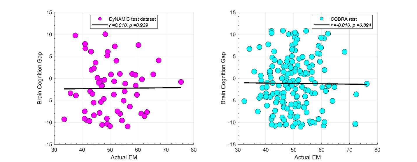
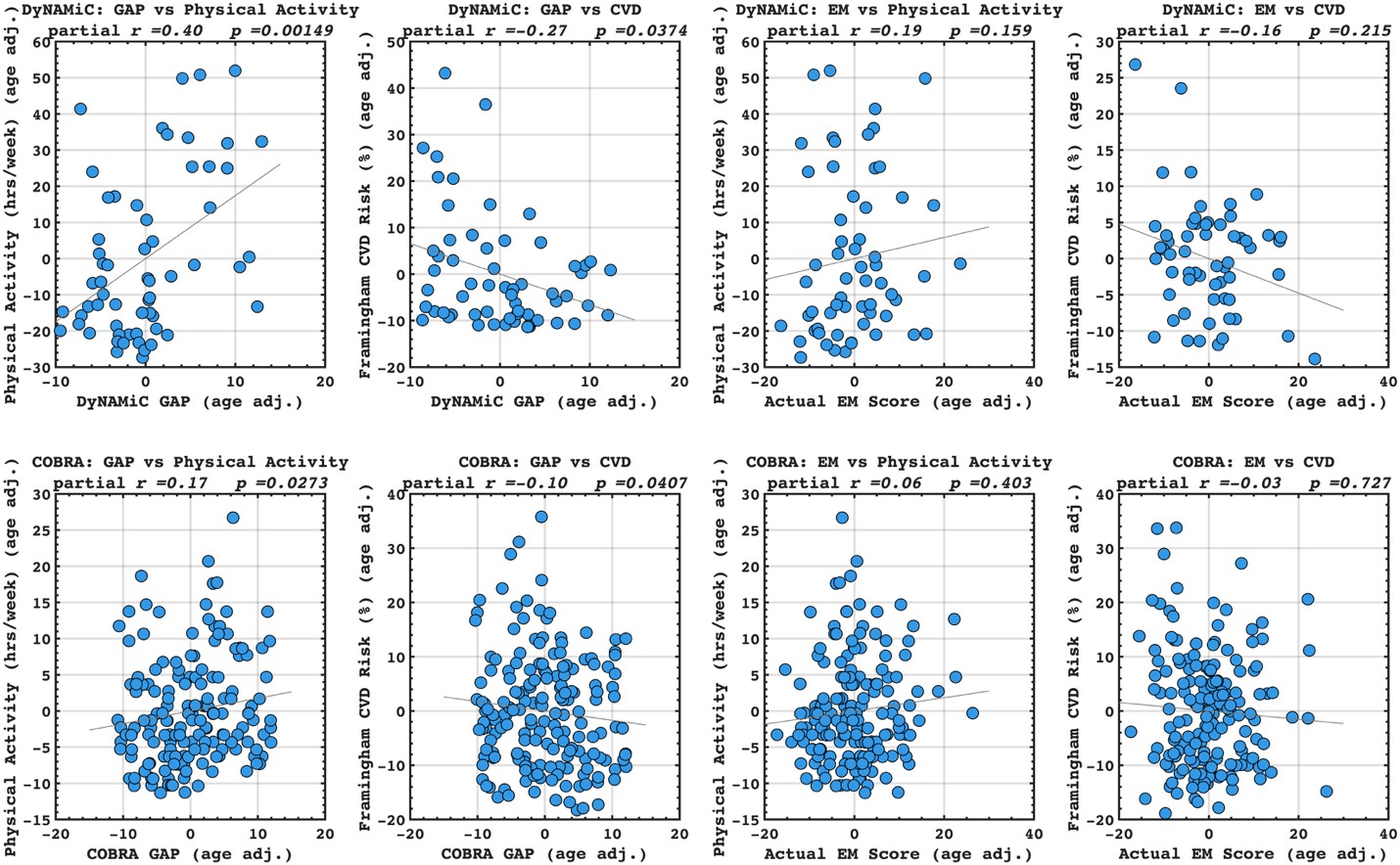
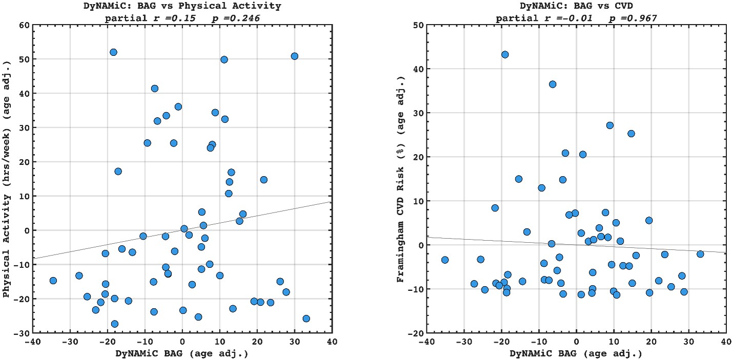
We thank the reviewer for raising this important point. In response to their request, we first examined the relationship between the BCG and the cognitive measure itself. We did not find any significant relationship in either the DyNAMiC sample (r =0.01, p =0.939) or the COBRA sample ((r =0.01, p=0.894) (see Author response image 1).
Author response image 1.
We then conducted additional analyses, splitting the sample into high and low EM performers, and compared their levels of physical activity and Framingham cardiovascular disease (CVD) risk scores. We found no significant difference in physical activity (DyNAMiC: p =0.56, 95% CI: –14.99 - 8.13; COBRA: p =0.29, 95% CI: –3.54 - 1.05) or Framingham CVD risk score (DyNAMiC: p =0.11, 95% CI: –1.08 - 10.72; COBRA: p =0.41, 95% CI: –1.86 - 4.58) between high and low EM perfprmers. Given the significant difference in physical activity and Framingham CVD risk score between positive and negative BCG groups, our results support that BCG provides unique information, beyond the observed cognitive measure (episodic memory score), regarding factors that contribute to cognitive resilience. These results have been added to Section 2.4, and Figure 3 has been updated.
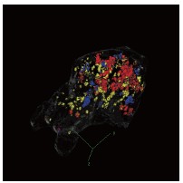
Some of the imaging findings require deeper analysis. For Figure 1f - Which default mode regions have high salience? DMN is a huge network with subregions having differing functions.
Grad-CAM provides a coarse, gradient-based attribution that reflects how the learned feature maps contribute to the model output. It is not designed to produce specific input-level interpretations, such as symmetric edge-wise importance values. Therefore, the primary interpretation remains at the network level rather than at the level of individual FC edges.
Along the same lines, were the striatal D1R findings regionally specific at all? It would be informative to test whether the three nuclei (Accumbens, Caudate, Putamen) and/or voxelwise models would show something above and beyond what is achieved from averaging D1R across the striatum. What about cortical D1R, which is highly abundant, strongly associated with cognitive (especially WM) performance, and has much unique variance beyond striatal D1R? https://www.science.org/doi/full/10.1126/sciadv.1501672. The PET findings are one of the unique strengths of this paper and are underexplored. It's also unclear if the measure of brain entropy should simply be averaged across all regions.
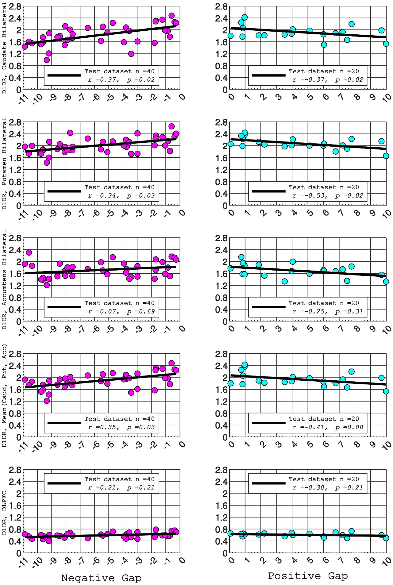
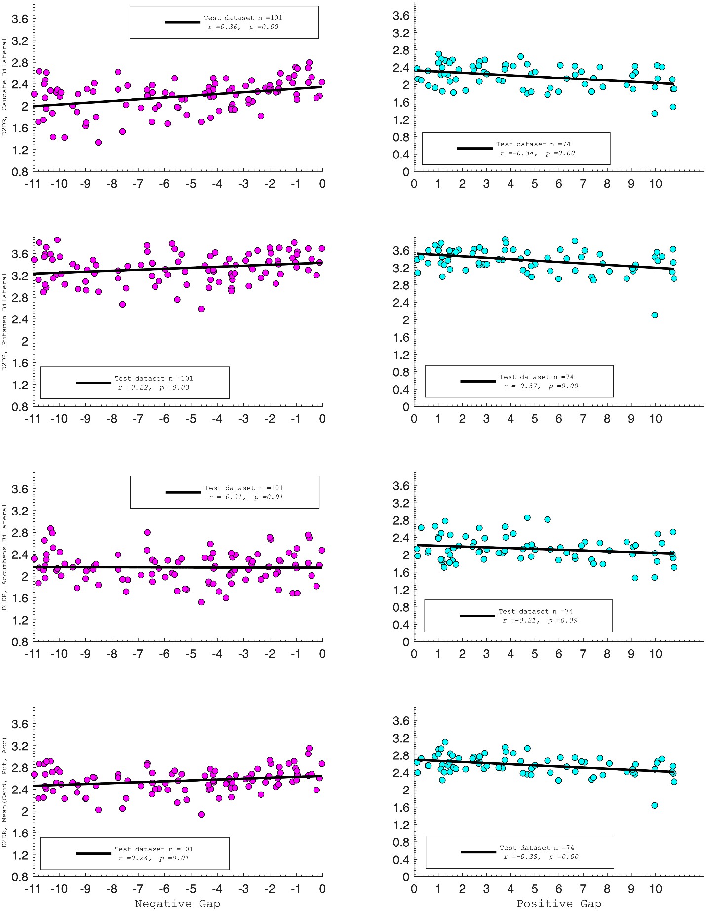
In this study, we focused on D1DR/ D2DR averaged across the caudate and putamen, which has been reported in our previous work to be more strongly associated with cognitive functions (Johansson et al., 2023, Nyberg et al., 2016), compared to the nucleus Accumbens, which tends to show lower D1DR/D2DR levels and limited association with these cognitive domains. Following the Reviewer’s suggestion, we examined regional variations and found that while both caudate and putamen D1DR showed significant associations with BCG, there were no significant associations for D1DR in the nucleus accumbens or DLPFC with BCG. For D2DR, we observed a significant association between caudate/putamen D2DR and BCG.
D1DR:
Partial correlation between:
Caudate_Bilateral vs. NegGap, (r =0.37, p =0.02
Putamen_Bilateral vs. NegGap, r =0.34, p =0.03
Accumbens_Bilateral vs. NegGap, r =0.07, p =0.69
Mean (LRCaud, LRput, LRacc) vs NegGap, r =0.35, p =0.03
DLPFC_Bilateral vs NegGap, r =0.21, p =0.21
Striatum_Bilateral (Mean (LRCaud, LRput)) vs. NegGap, r =0.40, p =0.01
Caudate_Bilateral vs. PosGap, r=–0.37, p=0.02
Putamen_Bilateral vs. PosGap, r=–0.53, p=0.02
Accumbens_Bilateral vs. PosGap, r=–0.25, p=0.31
Mean (LRCaud, LRput, LRacc) vs PosGap, r=–0.41, p=0.08
DLPFC_Bilateral vs. PosGap, r=–0.30, p=0.21
Striatum_Bilateral (Mean (LRCaud, LRput)) vs. PosGap, r=–0.49, p=0.03
Author response image 2.
D2DR:
Correlation between:
Caudate_Bilateral vs. NegGap, r=0.36, p=0.0003
Putamen_Bilateral vs. NegGap, r=0.22, p=0.03
Accumbens_Bilateral vs. NegGap, r= –0.01, p=0.91
Mean (LRCaud, LRput, LRacc) vs PosGap, r= –0.24, p=0.01
Striatum_Bilateral vs. NegGap, r=0.39, p=0.0001
Caudate_Bilateral vs. PosGap, r= –0.34, p=0.004
Putamen_Bilateral vs. PosGap, r= –0.37, p=0.002
Accumbens_Bilateral vs. PosGap, r= –0.21, p=0.09
Mean (LRCaud, LRput, LRacc) vs PosGap, r= –0.38, p=0.001
Striatum_Bilateral vs. PosGap, r= –0.49, p=0.0001
We have added the following sentence to the Results section to highlight these regional differences in D1DR/D2DR in relation to BCG.
“Both D1DR and D2DR availability in the striatum were associated with BCG, such that lower dopamine receptor availability was linked to a greater behavioral-cognitive gap. However, these associations varied by region. For D1DR, significant correlations with BCG were observed in the caudate (positive gap: r = –0.37, p =0.02; negative gap: r= 0.37, p =0.02) and putamen (positive gap: r = –0.53, p=0.02; negative gap:r=0.34, p=0.03), but not in the nucleus accumbens (positive gap: r= –0.25, p= 0.31; negative gap: r =0.07, p=0.69) or the DLPFC (positive gap: r = –0.30, p=0.21; negative gap: r =0.21, p=0.21). For D2DR, both caudate (positive gap: r = –0.34, p=0.004; negative gap: r =0.36, p=0.0003) and putamen (positive gap: r = –0.37, p=0.002; negative gap: r =0.22, p=0.03) showed significant associations with BCG.”
Author response image 3.
It is not clear from the text that the authors met the preconditions for mediation analysis (that is, demonstrating significant correlations between D1R and entropy, in addition to the correlation with brain gap. The authors should report this as well.
This is a fair question. We recalculated entropy in the striatum, given that D1DR is more strongly expressed in this region and, therefore, reduced striatal D1DR may have a more pronounced impact on local entropy (as the reviewer suggested, it may not be appropriate to compute entropy across all brain regions). Our analyses showed that lower D1DR/D2DR levels were associated with higher entropy, which in turn was related to higher BCG.
DyNAMiC; negative gap:
Partial correlation between:
Entropy and D1DR, r = –0.33, p=0.04.
Entropy and NegGap, r = –0.36, p=0.03.
DyNAMiC; positive gap:
Partial correlation between:
Entropy and D1DR, r = –0.56, p=0.01.
Entropy and PosGap, r r =0.47, p=0.04.
COBRA; negative gap:
Correlation between:
Entropy and D2DR, r = –0.22, p=0.03.
Entropy and NegGap, r = –0.27, p=0.007.
COBRA; positive gap:
Correlation between:
Entropy and D2DR, r = –0.26, p=0.03.
Entropy and PosGap, r = 0.25, p=0.03.
We have added these results under the result section 2.6. We have further updated Figure 4 in the revised manuscript, reporting these correlation results.
Was age controlled for in the mediation analysis? I would not consider this result valid unless that is the case.
We utilized the mediation package in R, and to control for a covariate age in the mediation analysis, we added age as a covariate in both the mediator model and the outcome model. The following information has been added in the method section in the revised version of the manuscript.
“To assess the statistical significance of this mediation effect, we employed the bootstrapping method as outlined by Preacher and Hayes (145) and age has been controlled for in all statistical analysis.”
The discussion section is long, but the authors would do better to replace some less helpful sections (e.g., the paragraph on methodological tweaks to parcellations and model alignment) with a couple of other important points, including:
(1) Discuss the 'sweet-spot' of movie watching for behavior prediction in the context of studies showing that task states 'quench' neural variability: https://journals.plos.org/ploscompbiol/article?id=10.1371/journal.pcbi.1007983. This may not be mutually exclusive of the discussion on dopamine and signal-to-noise ratio, but it would be helpful for the authors to discuss their potential overlap vs. unique contributions to the observed findings.
Thank you for the comment. We have now eliminated the section about methodological tweaks and extended the discussion on the sweet-spot of the task for behavioral prediction by referencing the paper that the reviewer suggested. Here comes the paragraph discussing this topic:
“Additionally, previous research showed that movie-watching alters the propagation of activity across cortical pathways (105), particularly within and between regions involved in audiovisual processing and attention. These alterations lead to a less segregated and more integrated network organization (106). Similarly, the n-back task has been associated with increased integration of task-positive cortico-cortical connectivity (104, 107) and striato-cortical connectivity (102). Our findings also suggest that certain task contexts strike an optimal balance between reducing neural variability and maintaining sufficient richness to capture individual differences. Prior work shows that task states quench neural variability, leading to a more reliable and predictable neural signal (108). In this context, movie watching may represent such a sweet spot constraining neural dynamics through shared audiovisual stimulation, while simultaneously engaging a broad range of cognitive processes that preserve individual differences.”
(2) The argument that dopamine signaling increases signal-to-noise ratio is based on some preclinical data as well as correlational data using fMRI with pharmacological challenges. It is less clear how PET-derived estimates of D1R and D2R availability equate to 'dopamine signaling' as it is thought of in this context. Presumably, based on these data, higher D1R or D2R availability would be related to greater levels of tonic dopaminergic signaling. However, in the case of the COBRA dataset with D2R estimates, those are based on raclopride -- which competes with endogenous dopamine for the D2 receptor. Therefore, someone with higher levels of endogenous dopamine signaling should theoretically have lower raclopride binding and lower D2R estimates. I'm not arguing that the authors' logic is flawed or that D1R and D2R are not good measures of dopamine signaling, but I'd ask the authors to dig into the literature and describe more direct potential links for how greater receptor availability might be associated with greater dopamine signaling (and hence lower entropy). Adding this to the discussion would be very valuable for PET research.
Thank you for raising this important point. We agree that D1R and D2R availability should not be taken as direct proxies of dopamine signaling. However, prior work has suggested meaningful associations between pre- and post-synaptic markers. For instance, a well-powered study demonstrated a significant correlation between D2R availability and dopamine synthesis capacity measured by FMT (Berry et al., 2018). This finding supports the idea that postsynaptic receptor markers may, under certain conditions, serve as an indirect proxy for dopaminergic signaling. Moreover, the number of dopamine-producing neurons innervating the striatum during development has been proposed to shape the structural maturation and arborization of dendrites (McAllister, 2000; Whitford et al., 2002), potentially providing a structural and functional basis for observed associations between pre- and post-synaptic measures.
At the same time, smaller-scale studies have yielded mixed findings, reporting either non-significant associations (Heinz et al., 2005; Kienast et al., 2008) or negative correlations (Ito et al., 2011). Importantly, the latter studies employed [18F]FDOPA to index dopamine synthesis, which has been argued to provide a less reliable estimate of synthesis capacity compared to FMT, as used in Berry et al. (2018). These inconsistencies underscore that the relationship between pre- and post-synaptic markers is not straightforward and requires further examination in larger, well-powered samples. The following paragraph has been added to the discussion.
“An important caveat is that D1DR and D2DR availability do not provide a direct measure of dopamine signaling. Instead, they reflect receptor availability, which interacts with endogenous dopamine in a complex manner. PET measures of D1R and D2R availability reflect the density of unoccupied dopamine receptors and the degree to which endogenous dopamine competes with radioligand binding. D2R binding potential is sensitive to competition from synaptic dopamine, such that higher ambient dopamine generally reduces tracer binding; D1R binding, however, is less affected by endogenous dopamine under physiological conditions, reflecting more directly receptor expression levels. Previous studies demonstrated a significant association between D2R availability and dopamine synthesis capacity measured by FMT (117, 118), suggesting that postsynaptic receptor markers may, under certain conditions, serve as a proxy for dopaminergic signaling. Developmental factors, such as the number of dopamine-producing neurons innervating the striatum, may further influence the structural and functional relationship between pre- and post-synaptic markers. By contrast, smaller studies have reported non-significant (119, 120) or negative (121) associations, although these studies relied on [18F]FDOPA, which is considered a less precise index of dopamine synthesis than FMT. Taken together, these reports indicate that the relationship between pre- and post-synaptic markers is complex and not necessarily linear. Accordingly, our observation that lower receptor availability is associated with greater neural variability should not be interpreted as direct evidence of weaker dopaminergic signaling, but rather as reflecting the interplay between receptor density and endogenous dopamine occupancy, particularly in the case of D2DR.”
Reviewer #2 (Public review):
Summary:
The authors developed a deep learning model based on a DenseNet CNN architecture to predict two cognitive functions: working memory and episodic memory, from functional connectivity matrices. These matrices were recorded under three conditions: during rest, a working memory task, and a movie, and were treated as images for the CNN algorithm. They tested their model's performance across different conditions and a separate dataset with a different age distribution (using the same MRI scanner, scanning configurations, and cognitive tests). They also calculated the "brain cognition gap" based on the model trained on resting functional connectivity to predict working memory. Extending from the commonly used index "brain age," the brain cognition gap was defined as the difference between the working memory score predicted by their model (predicted working memory) and the working memory score based on the working memory test itself (observed working memory). This brain cognition gap was found to be associated with physical activity, education, and cardiovascular risk. The authors also conducted additional mediation tests to examine whether regional functional variability mediated the relationship between PET-derived measures of dopamine and the brain cognition gap.
Strengths:
The major strength of this manuscript is the extensive effort the authors have put into creating a new 'biomarker' that links deep learning with fMRI, PET, physical activity, education, and cardiovascular risk across two studies. This effort is impressive.
Weaknesses:
There are several weaknesses in the current methods and results, making many of the claims unconvincing. These weaknesses include:
(1) The lack of baseline models to benchmark the predictive performance of their DenseNet models.
(2) The inappropriate calculation of the brain cognition gap due to the lack of control for regression-toward-the-mean and the influence of the working memory itself (a common practice in brain age studies).
(3) The lack of benchmarking of the brain cognition gap against the 'corrected' brain age gap and the direct prediction of physical activity, education, and cardiovascular risk.
(4) Minimal justification for their PET mediation analysis.
We appreciate the reviewer’s constructive comments on the strengths and weaknesses of our study. In this revised version, we’ve addressed the concerns regarding the calculation of the brain-cognitive gap, clarified the unique variance that the brain-cognitive gap contributes beyond cognition itself, and provided additional justification for the PET mediation analysis. For the lack of a baseline model, it is important to highlight that our aim has never been to compare the predictive power of different deep learning or machine learning approaches. Therefore, the text in the introduction and discussion has been amended to avoid miscommunication on this topic.
Regarding the impact of the work on the field and the utility of the methods and data to the community, I see its potential. However, addressing all the weaknesses listed above is crucial and likely to change the conclusions of the results.
It is important to note that many statements in the manuscript are overstated, making the contribution of the manuscript seem exaggerated.
We have run additional analysis based on the reviewer’s suggestions. The effect sizes and statistical values were adjusted due to the corrections; the overall conclusions remain largely consistent. The relationships between the brain-cognition gap and key factors such as physical activity, and cardiovascular risk persisted. We have updated the manuscript accordingly and revised the relevant sections to reflect these refinements and the resulting interpretations.
For instance, the abstract claims "there is a lack of objective biomarkers to accurately predict cognitive function," and the discussion states, "across various studies, the correlation between predicted and actual fluid intelligence typically hovers around 0.25 (98-100)." However, a meta-analysis by Vieira and colleagues (2022 https://doi.org/10.1016/j.intell.2022.101654) found over 37 studies up to 2020 predicting cognitive abilities from fMRI with machine learning, with 24 studies published in 2019-20 alone. Since 2020, with the rise of machine learning and AI, even more studies have likely been published on this topic, all claiming to show objective biomarkers to accurately predict cognitive function. Vieira and colleagues also found an average performance of these objective biomarkers in predicting general cognition at r = .42, similar to what was found in this manuscript. Based on this alone, it is unclear how novel or superior their method is without a proper systematic benchmark.
We appreciate the opportunity to clarify our study’s contribution relative to prior work. We have revised the introduction and discussion to highlight the contribution of other methods when it comes to biomarkers. As for the comment related to the work by Vieira and colleagues, Vieira et al. (2022) indeed present a comprehensive meta-analysis of studies predicting general and fluid intelligence using neuroimaging and machine learning. However, there are two critical differences between ours verus previous work:
Target Cognitive Domains:
Our study does not focus on general or fluid intelligence, but rather on comprehensive EM (3 tests) and WM (3 tests), two distinct cognitive domains that are critically important for aging research. These distinct abilities, in this context (measured by three independent tests to boost the reliability) are less frequently studied as predictive targets in the existing fMRI-ML literature, particularly using deep learning methods.
Critically, our study explicitly compares predictive power across different cognitive states (rest, movie watching, n-back), with the aim of identifying the states that best capture individual differences across domains. Thus, our goal was not to propose a universally superior prediction model, but rather to test how brain state influences predictive utility for WM and EM using a deep learning approach.
Our primary objective is to test how brain state influences the ability of functional connectivity to predict domain-specific cognitive performance, using a deep learning framework. As now stated explicitly in the revised manuscript, this objective is operationalized through three clearly defined aims:
(1) To compare the predictive utility of functional connectomes derived from different brain states (resting state, movie watching, and n-back task) for EM and WM;
(2) To introduce and evaluate a brain-cognition gap as a marker of individual differences beyond chronological age; and
(3) To examine the contribution of dopaminergic integrity to variability in connectome uniqueness and brain-cognition gaps.
We have revised the manuscript text to make this focus clearer and to avoid any misinterpretation of our aims. Specifically, we removed statements in the Discussion that could be read as suggesting that our deep learning approach outperforms prior machine learning methods. While we compared our model with the connectome predictive modeling (CPM) approach and observed better performance with our deep learning framework for some of the prediction models, we did not conduct a comprehensive benchmark across all available machine learning methods nor was this the aim of the present study. Accordingly, we have adjusted the text to avoid implying methodological/biomarker superiority beyond the scope of our analyses.
Modeling Approach:
While Vieira et al. show that the majority (76%) of prior studies used linear modeling approaches, including CPM and penalized regressions, these models are often vulnerable to overfitting, especially when applied to high-dimensional fMRI data. Our use of a DenseNet-based CNN architecture is motivated by the need to leverage inductive biases suited to functional connectivity data, and we evaluate this approach across multiple cognitive tasks and independent datasets.
Vieira and colleagues report that studies predicting general intelligence from fMRI (particularly from the HCP dataset) average around r =0.42, while those predicting fluid intelligence average around r =0.15. Our original claim about the correlation hovering around 0.25 is therefore not incorrect – and aligns with the Vieira meta-analysis. We have, however, nuanced this statement in the manuscript, now stating that correlations are higher for general intelligence than fluid intelligence.
Altogether, we considered the reviewer’s comments and therefore conducted a careful revision of the manuscript text to moderate and clarify statements that may have come across as overstated. We have refined the language throughout the Introduction and Discussion sections to better align with the strength of the evidence and the scope of our contributions. A few examples are:
“Our study explicitly compares predictive power across different cognitive states (rest, movie watching, n-back), with the aim of identifying the states that best capture individual differences across domains. The relative performance of deep learning and other non-linear approaches depends on multiple factors, including sample size, model architecture, feature representation, and domain-specific characteristics of the prediction target. In this context, deep learning was employed as a flexible framework capable of modeling high-dimensional functional connectivity patterns across cognitive states, rather than as a claim of inherent methodological superiority. Thus, our goal was not to propose a universally superior prediction model, but rather to test how brain state influences predictive utility for WM and EM using a deep learning approach.”
Also in page 14.
“Our study introduces a deep neural network architecture that features dense connections and incorporates an attentional mechanism. While our findings demonstrate that a deep learning framework can provide reasonable predictive accuracy, it is important to note that other machine learning approaches (e.g., tree-based models) may offer comparable predictive power, as suggested by prior benchmarking work (29, 30).”
Similarly, the authors claim superior performance of deep learning and mischaracterize machine learning algorithms: "In particular, deep neural networks (DNN) methods have been successfully applied to behavioral and disease prediction (24-26), and have been found to outperform other machine learning approaches (27-29)," and "Deep learning approaches overcome the limitation of predictive techniques that solely rely on linear associations between connectivity and behavioral phenotypes (17)." However, the superiority of deep learning is debatable. Studies show comparable performance between machine learning (such as kernel regression) and deep learning (such as fully-connected neural networks, BrainNetCNN, Graph CNN (GCNN), and temporal CNN), e.g., He and colleagues (2019) and Vieira and colleagues (2024) https://doi.org/10.1016/j.neuroimage.2019.116276 and Vieira and colleagues' https://doi.org/10.1101/2024.03.07.583858.
We agree that the performance gap between traditional machine learning models and deep learning (which is a subcategory of machine learning) in neuroimaging is debatable and task-dependent. Indeed, both He et al. (2019) and Vieira et al. (2024) offer evidence that kernel regression can achieve performance on par with deep learning models, applied to appropriate datasets.
We have therefore nuanced the statements in the revised version of the manuscript as follows:
Introduction:
“In particular, deep neural networks (DNN) methods have been successfully applied to behavioral and disease prediction (24-26), and were initially expected to outperform other machine learning approaches (27-29). However, this superiority remains debatable, as recent studies have reported comparable performance between DNNs and traditional methods (He et al.,2019; Vieira et al.,2024). Accordingly, the present study does not aim to benchmark deep learning against traditional machine learning approaches, but instead uses a consistent predictive framework to examine how brain state influences the utility of FC for cognitive prediction.”
“Deep learning approaches offer a flexible modeling framework capable of capturing complex non-linear associations in high-dimensional data with potentially less sensitivity to training on a smaller subsample (Vieira et al., 2024)”.
Discussion:
We agree that traditional methods, such as kernel-based models, tree ensembles, and non-linear SVRs, can also effectively capture such relationships. The relative performance of our model and other non-linear approaches depends on several factors, including data size, model architecture, and domain-specific considerations. We have included additional explanations in the discussion to address this.
Moreover, many non-deep learning predictive techniques are non-linear, e.g., XGBoost, CatBoost, random forest, kernel ridge, and support vector regression with non-linear kernels (such as RBF and polynomial). Thus, stating that machine learning can only model linear relationships is incorrect. Moreover, for the small amount of data the authors had, some might argue that a linear algorithm might be more appropriate to balance the bias-variance trade-off in prediction. Again, without a proper systematic benchmark, it is unclear how well their DenseNet algorithm performs compared to other algorithms.
Thank you for bring this up. We have now removed statements implying that machine learning can only model linear relationship.
Regarding the Brain Age literature, the authors also misinterpreted recent findings: "However, a recent study suggests that brain age predictions contribute minimally compared to chronological age for explaining cognitive decline (65), implying that cognitive predictions are more reliable." In this study, Tetereva and colleagues (2024) (https://doi.org/10.7554/eLife.87297.4) showed that non-deep-learning machine learning can make good predictions from MRI on both chronological age (with r up to .88) and fluid cognition (with r up to .627). Using the combination of functional connectivity matrices across rest and tasks to predict fluid cognition, they found performance at r = .565, comparable to what was found in the current manuscript with deep learning. Nonetheless, while brain age predicted chronological age well (and brain cognition predicted fluid cognition well), it was problematic to predict fluid cognition from brain age. They showed that, because brain age, by design, shared so much common variance with chronological age, brain age and chronological age captured the same variance of fluid cognition. When chronological age was controlled for in the prediction of fluid cognition, brain age no longer had high predictive ability. In the case of the current manuscript, the brain cognition gap is not appropriately controlled for cognition (to be more precise, a working memory score). I expect the performance in predicting physical activity, education, and cardiovascular risk will drop dramatically once cognition is controlled for. There are at least two ways to control cognition according to Tetereva and colleagues' study (see more in the recommendations).
We thank the reviewer for breaking down the findings in the study by Tetereva and colleagues (2024). It was not our intention to suggest that Tetereva et al. showed brain age has little predictive value in general. Our understanding of the findings reported in that study is on par with the reviewers’ clarifications. We have now revised the introductions to avoid any misunderstanding:
“A recent study demonstrated that while brain age can predict chronological age with high accuracy from MRI, its utility for predicting cognition is limited. Specifically, Tetereva and colleagues (2024) showed that brain age strongly tracks chronological age and that brain cognition (using functional connectivity) can predict fluid cognition. Yet, when used to predict cognition, brain age largely overlapped with chronological age, such that controlling for chronological age eliminated the predictive contribution of brain age. This finding suggests that brain-age models may provide little unique explanatory power for cognitive decline beyond what is already captured by chronological age. Building on this observation and extending the concept of a brain-age gap to a brain-cognition gap (BCG, defined as the discrepancy between predicted and observed cognitive performance), we propose that a BCG may serve as an informative marker of individual differences.”
In addition, in response to the first comment from Reviewer 1, we have extended our results in the manuscript. We first showed that BCG is not significantly associated with cognition itself (see Author response image 1). Moreover, we conducted additional analyses, splitting the sample into high and low EM performers, and compared their levels of physical activity and Framingham cardiovascular risk scores. We found that no significant difference in physical activity (DyNAMiC: p =0.56, 95% CI: -14.99 – 8.13; COBRA: p =0.29, 95% CI: -3.54 – 1.05) or Framingham CVD risk score (DyNAMiC: p =0.11, 95% CI: -1.08 – 10.72; COBRA: p =0.41, 95% CI: -1.86 – 4.58) between high and low EM performers. Given the significant difference in physical activity and Framingham CVD risk score between positive and negative BCG groups, our results support that BCP provides unique information, beyond cognitive measures, regarding factors that contribute to cognitive resilience. This text has been added into the result section, and Figure 3 has been updated in the manuscript.
The authors mentioned, "The third aim of the current study is to uncover the contribution of dopamine (DA) integrity to brain-cognition gaps." However, I fail to see how mediation analysis would test this. The authors also mentioned, "Insufficient DA modulation can affect neurocognitive functions detrimentally (69, 74, 76-78)." They should test if DA levels are related to working memory scores in their study, and if so, whether the relationship is mediated by the "corrected" brain-cognition gaps. Note see more on the recommendation for the calculation of the "corrected" brain-cognition gaps.
Our mediation was not designed to test whether DA predicts episodic memory performance directly, nor whether BCG mediates such a relationship. Instead, we specifically investigated whether the effect of DA on BCG operates through functional variability, the theoretical framework emphasizing the role of DA on neuronal grain and signal-to-noise ratio (see our recent work in Korkki et al., 2025). We agree that future work could extend our approach by directly examining whether BCG mediates the link between DA and cognitive outcomes. However, in the present study, our primary focus was on testing the mechanistic pathway of DA → entropy → BCG.
In line with this aim, we found that lower DA receptor availability was associated with larger BCGs (Figure 4). We then asked whether this relationship is mediated by functional signal variability, such that lower DA is linked to reduced signal-to-noise ratio (i.e., greater entropy), which in turn contributes to less reliable prediction of cognition and, consequently, larger BCGs. Our mediation analysis supports this pathway (please see also our reply to Reviewer 1, Comment 6).
Reviewer #3 (Public review):
Summary:
This paper by Esmaeili and co-authors presents a connectome prediction study to predict episodic memory and relate prediction errors to other phonotypic variables.
Strengths:
(1) A primary and external validation dataset.
(2) Novel use of prediction errors (i.e., brain-cognitive gap).
(3) A wide range of data was investigated.
Weaknesses:
(1) Lack of comparisons to other methods for prediction.
(2) Several different points are being investigated that don't allow any particular one to shine through.
(3) Some choices of analysis are not well-motivated.
(4) How do the n-back connectomes perform for prediction if the authors do not regress task activations from the n-back task?
We thank the reviewer for raising these important points. For the lack of comparisons to other methods, it is important to highlight that our aim has never been to compare the predictive power of different deep learning or machine learning approaches. Rather, our primary objective was to test how brain state influences the ability of functional connectivity to predict domain-specific cognitive performance, using a deep learning framework.Therefore, the text in the introduction and discussion has been amended to avoid miscommunication on this topic.
We chose to regress out task-evoked activations based on prior work demonstrating that failing to do so can produce spurious but systematic inflation of task functional connectivity estimates (Cole et al., 2019). In that study, as well as subsequent reports (e.g., Gao et al., 2020; Gonzalez-Castillo & Bandettini, 2018), connectomes derived without activation regression tended to capture task-evoked coactivations rather than background task functional interactions, which can artificially boost predictive performance but limit interpretability (whether it is co-activation or intrinsic connectivity during an entire goal-oriented task) and generalizability. For this reason, our analyses focused on the more conservative approach of regressing out task activations. Accordingly, we compared predictive performance only under this preprocessing strategy.
We have added the following sentence to clarify this in the method: “To avoid spurious inflation of task functional connectivity by task-evoked activations, we regressed out task activation patterns from the n-back data prior to estimating functional connectivity, following recommendations by Cole et al. (2019) and related work.”
(5) I am a little concerned about overfitting with the convolutional neural net. For example, the drop-off in prediction performance in the external sample is stark. How does the deep learning approach used here compare to something simpler, like a connectome-based predictive model or ridge regression?
(6) It may be nice to try the other models in the validation dataset. This would also provide a sense of the overfitting that may be going on with overfitting.
We thank the reviewer for raising this point. The prediction performance indeed dropped for episodic memory when models trained on the DyNAMiC sample were applied to the COBRA sample, whereas performance for working memory remained nearly identical across datasets. Moreover, our prediction power is on par with previous studies reporting reliable prediction of intelligence using deep learning approach (Vieira et al., 2021; Fan et al.,2020). While we compared our model with the connectome predictive modeling (CPM) approach and observed better performance with our deep learning framework, we did not conduct a comprehensive benchmark across all available machine learning methods nor was this the aim of the present study.
We have revised the manuscript text to make this focus clearer and to avoid any misinterpretation of our aims. Specifically, we removed statements in the Discussion that could be read as suggesting that our deep learning approach outperforms prior machine learning methods. Finally, We have added the following paragraph to the discussion:
“Our study used a deep neural network architecture that features dense connections and incorporates an attentional mechanism. While our findings demonstrate that a deep learning framework can provide reasonable predictive accuracy, it is important to note that other machine learning approaches (e.g., tree-based models) may offer comparable predictive power, as suggested by prior benchmarking work (29, 30). Our study explicitly compares predictive power across different cognitive states (rest, movie watching, n-back) to identify the states that best capture individual differences across domains. The relative performance of deep learning and other non-linear approaches depends on multiple factors, including sample size, model architecture, feature representation, and domain-specific characteristics of the prediction target. In this context, deep learning was employed as a flexible framework capable of modeling high-dimensional functional connectivity patterns across cognitive states, rather than as a claim of inherent methodological superiority. Thus, our goal was not to propose a universally superior prediction model, but rather to test how brain state influences predictive utility for WM and EM using a deep learning approach.”
(7) While predictive models increase the power over association studies, they still require large samples to prevent overfitting. Do the authors have a sense of the power their main and external validation sample sizes provide?
We thank the reviewer for this important point. Our main sample size, together with the external validation in COBRA, is moderate for deep learning applications. To reduce the risk of overfitting, we employed several strategies, including external validation, early stopping, dropout, and regularization. As noted, performance for episodic memory decreased in the external sample, which we acknowledge, but key associations such as the link between BCG and resilient factors remained significant. Importantly, prediction of working memory was maintained across datasets, reducing the likelihood that the observed findings are driven by overfitting. We have added a statement in the Discussion to reflect on the limitations of sample size and the implications for generalizability.
We added the following sentence to the discussion:
“We acknowledge that our main and validation samples are moderate in size for deep learning, which constrains statistical power and generalizability. Although external validation, early stopping, dropout, and regularization help mitigate overfitting, larger samples will be needed in future work to fully establish the robustness of these predictive models.”
(8) I am not sure that the Mann-Whitney is the correct test for comparing the distributions of prediction performances. The distributions are dependent on each other as they are each predicting the same outcomes. Using the typical degrees of freedom formula would overestimate the degrees of freedom.
We appreciate the reviewer’s comment and agree that applying statistical tests directly to bootstrapped samples can lead to inflated or misleading p-values, as the degrees of freedom are determined by the number of bootstrap iterations rather than the actual number of independent observations.
In our analysis, the Mann-Whitney U test was applied to 1000 bootstrapped correlation coefficients (r) for each model. While this number is relatively low and was chosen to limit overestimation of significance, we recognize that these bootstrapped samples are not independent, and thus the use of a Mann-Whitney U test can still be problematic. To address this concern, we have revised our statistical analysis. Rather than applying the Mann-Whitney U test to the bootstrapped r distributions, we now compute the difference in correlation coefficients (Δ r = r<sub>actual</sub> − r<sub>rest</sub>) for each bootstrap iteration. We then calculate a 95% confidence interval for Δr. If this interval does not include zero, we consider the difference statistically significant. This approach avoids artificially inflating the sample size and adheres more closely to proper statistical inference.
We have updated the Methods (the following text) and Results sections accordingly and clearly stated the limitations regarding the degrees of freedom for all tests.
“For the bootstrap-based comparison of model performance (bootstrap resampling with 1000 iterations), no test statistic with an associated degree of freedom is reported. Instead, statistical inference is based on the bootstrap distribution of the difference in correlation coefficients (Δr) and its 95% confidence interval. As bootstrap confidence-interval–based inference does not rely on an analytic sampling distribution, degrees of freedom are not defined for this procedure.” This has now been explicitly stated in the Methods section to avoid ambiguity.
In the result section, we have reported with corresponding CI.
(9) The brain cognition gap is interesting. It is very similar conceptually to the brain age gap. When associating the brain age gap with other phenotypes, typically age is regressed from the brain age gap and the other phenotype. In other words, age is typically associated with a brain age gap as individuals at the tail ages often show the largest gaps. Is the brain cognition gap correlated with episodic memory and do the group differences hold if episodic memory is controlled for?
We thank the reviewer’s comment regarding the relationship between the brain cognition gap and episodic memory.
Since this question was raised by all reviewers, we have conducted additional analyses. We did find that BCG is independent from the cognitive measure and provided additional information, beyond cognition alone, about factors contributing to resilience. Please visit our response to the first comment of Reviewer 1.
(10) I have the same question for the dopamine results. Particularly, in the correlations that are divided by brain cognition gap sign. I could see these types of patterns arise due to a correlation with a third variable.
For dopamine results, we explored whether age or cognition alone might confound the dopamine–brain cognition gap relationships. However, neither was significantly correlated with the brain cognition gap groups. The associations remained significant after controlling for age, suggesting that the observed patterns are not likely due to these potential third-variable confounder. This is also inline with our observation of significant associations between DA and GAP in an age-homogeneous COBRA sample. That said, we found that entropy, indeed, mediates the direct link between DA and BAG, suggesting that individuals with lower DA exhibit greater regional variability, and in turn larger BCG.
These results have now been embedded into the manuscript. We also highlighted that age has been controlled for in reported correlation and mediation analyses.
Recommendations for the authors:
Reviewing Editor Comment:
We particularly recommend that the authors: (a) compare the performance of their deep learning model with other baseline models, and (b) adjust for cognitive performance within the brain-cognition gap. These steps would strengthen the evidence base.
We thank the editor for their comments. As for the first comments, our study explicitly compares predictive power across different cognitive states (rest, movie watching, n-back), with the aim of identifying the states that best capture individual differences across domains. Thus, our goal was not to propose a universally superior prediction model, but rather to test how brain state influences predictive utility for WM and EM using a deep learning approach. We have revised the manuscript text to make this focus clearer and to avoid any misinterpretation of our aims. Specifically, we removed statements in the Discussion that could be read as suggesting that our deep learning approach outperforms prior machine learning methods. While we compared our model with the connectome predictive modeling (CPM) approach and observed better performance with our deep learning framework, we did not conduct a comprehensive benchmark across all available machine learning methods, nor was this the aim of the present study. Accordingly, we have adjusted the text to avoid implying methodological superiority beyond the scope of our analyses. Finally, we have added the following paragraph to the discussion:
“Our study used a deep neural network architecture that features dense connections and incorporates an attentional mechanism. While our findings demonstrate that a deep learning framework can provide reasonable predictive accuracy, it is important to note that other machine learning approaches (e.g., tree-based models) may offer comparable predictive power, as suggested by prior benchmarking work (29, 30).
Our study explicitly compares predictive power across different cognitive states (rest, movie watching, n-back) to identify the states that best capture individual differences across domains. The relative performance of deep learning and other non-linear approaches depends on multiple factors, including sample size, model architecture, feature representation, and domain-specific characteristics of the prediction target. In this context, deep learning was employed as a flexible framework capable of modeling high-dimensional functional connectivity patterns across cognitive states, rather than as a claim of inherent methodological superiority. Thus, our goal was not to propose a universally superior prediction model, but rather to test how brain state influences predictive utility for WM and EM using a deep learning approach.”
As for the second comment, we followed the instructions by Reviewer 1. In response to their request, we first examined the relationship between the Brain-Cognitive Gap (BCG) and the cognitive measure itself. Surprisingly, we did not find any significant relationship in either the DyNAMiC sample (r =0.01, p =0.939) or the COBRA sample (r =0.01, p =0.89) (see Author response image 1).
We then conducted additional analyses, splitting the sample into high and low EM performers, and compared their levels of physical activity and Framingham cardiovascular disease (CVD) risk scores. We found no significant difference in physical activity (DyNAMiC: p =0.56, 95% CI: –14.99 - 8.13; COBRA: p =0.29, 95% CI: –3.54 - 1.05) or Framingham CVD risk score (DyNAMiC: p =0.11, 95% CI: –1.08 - 10.72; COBRA: p =0.41, 95% CI: –1.86 - 4.58) between high and low EM perfprmers. Given the significant difference in physical activity and Framingham CVD risk score between positive and negative BCG groups, our results support that BCG provides unique information, beyond the observed cognitive measure (episodic memory score), regarding factors that contribute to cognitive resilience. These results have been added to Section 2.4, and Figure 3 has been updated.
Reviewer #1 (Recommendations for the authors):
(1) The top and bottom triangles of the saliency maps, particularly in Figure 2, do not look symmetrical (this is most notable in the hotspot representing the between-network correlation of DMN and FPN). What is going on here? Was the image compressed or altered in some way, or is this a visual artifact of the interpolation method?
We appreciate the reviewer’s insightful comment. Minor differences in the saliency maps between the upper and lower triangles of the FC matrix can arise due to several factors. For instance, Grad-CAM generates saliency maps at the resolution of the convolutional feature maps, which are then upsampled to match the input matrix dimensions. We initially used the default bilinear interpolation, which may have introduced slight asymmetries or blurring, resulting in interpolation artifacts. In response, we have reprocessed the saliency maps using spline interpolation in MATLAB. The updated saliency figures have been included in the revised version of the manuscript.
(2) Pages 11-12. Please make it explicit in the text that the brain gap-education association was not significant in the COBRA dataset.
Thanks for pointing this out. We added the following sentence to the discussion.
“Note that the association with education was significant only in the DyNAMiC sample and did not reach significance in the COBRA dataset.“
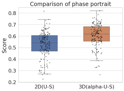
(3) Please overlay individual data points onto the boxplots in Figure 3 so that we can appropriately evaluate the data distributions.
Figure 3 has now been updated.
(4) Section 2.6: Was entropy calculated on movie-watching data, resting data, or all fMRI data? Please specify.
We thank the reviewer for pointing this out. We have updated the text (Section 2.6) to clarify that entropy was calculated from the resting-state data. We intended to examine the mediating role of regional variability in the relationship between dopamine and the BCG of the winning model for episodic memory. Because resting state and movie-watching were the winning conditions for EM prediction, but movie-watching was not available in COBRA, we focused on entropy during rest, which exists in both datasets.
(5) Was entropy during the resting state correlated with entropy during the task state, across individuals?
We agree this is an interesting question. However, investigating the correlation of entropy between rest and task states goes beyond the scope of the present study. Our aim here was to test whether regional variability mediates the effect of dopamine on the BCG. Specifically, we examined whether individuals with lower striatal D1DR show higher local variability, which in turn relates to less accurate prediction and a larger gap. We assessed both the relationship between D1DR and entropy and the association between entropy and the gap, and these results have now been added to the manuscript (see also our response to Reviewer 1’s public comment).
Reviewer #2 (Recommendation for authors):
(1) The lack of baseline models to benchmark the predictive performance of their DenseNet models makes their results hard to interpret. This problem is quite common across ML literature. For instance, many DL-based algorithms were developed for tabular data without proper benchmarking against other ML algorithms. When they were properly tested, most weren't better than many tree-based ML algorithms (e.g., https://proceedings.neurips.cc/paper_files/paper/2022/file/0378c7692da36807bdec87ab043cdadc-Paper-Datasets_and_Benchmarks.pdf). I can see that a similar problem might happen here.
For this particular manuscript, the authors made strong statements without doing a proper benchmark, e.g., from the discussion, "Indeed, the predictive power in the current study is stronger than for CPM-based predictions reported before." And "Unlike the BrainNet convolutional neural network, which focuses on staged transformations, our densely connected model promotes extensive feature reuse, possibly leading to more robust feature extraction." I hope to see the performance of the proposed algorithm against 1) other DL algorithms (e.g., fully-connected neural networks, BrainNetCNN, Graph CNN (GCNN), temporal CNN, GRU, and LSTM, see https://doi.org/10.1016/j.neuroimage.2019.116276 and https://doi.org/10.1002/hbm.26415), 2) ML algorithms (e.g., SVR with linear, RBF and polynomial kernels, Elastic Net, XGBoost, random forest, CPM), 3) data reduction algorithms (e.g., PCA regression, Partial Least Square). The results of this benchmark will substantiate the claims made by the authors.
Our goal was not to propose a universally superior prediction model, but rather to test how brain state influences predictive utility for WM and EM using a deep learning approach. We have revised the manuscript text to make this focus clearer and to avoid any misinterpretation of our aims. Specifically, we removed statements in the Discussion that could be read as suggesting that our deep learning approach outperforms prior machine learning methods. While we compared our model with the connectome predictive modeling (CPM) approach and observed better performance with our deep learning framework, we did not conduct a comprehensive benchmark across all available machine learning methods, nor was this the aim of the present study. Accordingly, we have adjusted the text to avoid implying methodological superiority beyond the scope of our analyses. Finally, we have added the following paragraph to the discussion:
“Our study used a deep neural network architecture that features dense connections and incorporates an attentional mechanism. While our findings demonstrate that a deep learning framework can provide reasonable predictive accuracy, it is important to note that other machine learning approaches (e.g., tree-based models) may offer comparable predictive power, as suggested by prior benchmarking work (29, 30). Our study explicitly compares predictive power across different cognitive states (rest, movie watching, n-back) to identify the states that best capture individual differences across domains. The relative performance of deep learning and other non-linear approaches depends on multiple factors, including sample size, model architecture, feature representation, and domain-specific characteristics of the prediction target. In this context, deep learning was employed as a flexible framework capable of modeling high-dimensional functional connectivity patterns across cognitive states, rather than as a claim of inherent methodological superiority. Thus, our goal was not to propose a universally superior prediction model, but rather to test how brain state influences predictive utility for WM and EM using a deep learning approach.”
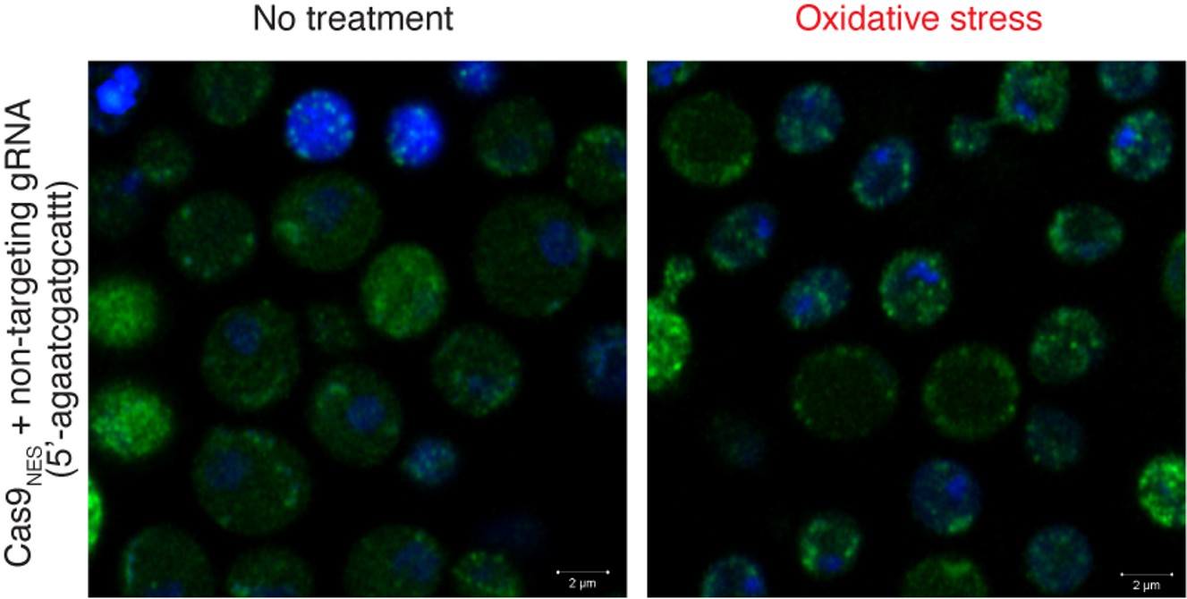
(2) From Figure 6b, it looks like the functional connectivity matrices were converted to different images, and each of the four images (in grey, blue, yellow, and red) was treated as a separate channel. What are these grey, blue, yellow, and red images?
In our study, the inputs to the deep learning models were subject-specific FC matrices of size 273×273. To augment the data, we created different versions of each FC matrix by reordering specific brain networks within the matrix. To visualize that the inputs were augmented, we used different color codings (grey, blue, yellow, and red) in Figure 6b. These colors were intended solely to represent different augmented versions of the same subject’s FC matrix. They were not treated as separate channels in the model. To avoid any confusion or misinterpretation, we have revised this part of the figure and now use only grey coloring to represent the augmented FC matrices.
(3) The differences in performance between within vs. outside studies might simply be due to the fact that the models trained from DyNAMiC captured the brain variation due to age, which is also related to cognitive abilities. I was wondering if age is controlled for, would performance be more similar across the studies? The authors should provide the performance of models that are controlled for age.
We initially conducted partial correlation between FC features and cognitive measures while controlling for age. This is further supported by the fact that the model trained on the age-heterogeneous DyNAMiC sample provided a fairly reasonable prediction in the age-homogeneous COBRA dataset, particularly for working memory (see figure 2d). Moreover, in our post hoc analyses, we additionally controlled for age when examining associations, for example, between GAP and dopamine measures.
(4) Related to point (3), from the discussion, "Validation outcomes thus affirm that the models, particularly those constructed from rest data, are robust to the particulars of the dataset." The performance dropped around half, so I am not sure if this conclusion is warranted.
We thank the reviewer for raising this point. The prediction performance indeed dropped for episodic memory when models trained on the DyNAMiC sample were applied to the COBRA sample, whereas performance for working memory remained nearly identical across datasets. Although both EM and WM are sensitive to age, the divergence in cross-dataset performance suggests that factors beyond age alone may contribute to these differences. To address this, we have revised the discussion as follows:
“Differences between the DyNAMiC and COBRA datasets make cross-dataset prediction a harder problem, as the age ranges of samples significantly vary, and prior studies highlight the importance of individual characteristics like age in predicting behavior from FC (33). In line with this, model performance decreased when predicting EM in the COBRA sample whereas prediction of WM remained largely unchanged. Thus, validation outcomes suggest that the models, particularly those predicting WM, show robustness across datasets, whereas the reduced EM performance highlights potential data-specific influences that limit generalizability.”
(5) Please report the degree of freedom in all of the statistical analyses. Was the Mann-Whitney U test done on the bootstrapped r? If so, the degree of freedom was arbitrarily set by the number of bootstrapping, and hence the p-value can be higher or lower depending on the number of bootstrapping. This could lead to misleading conclusions.
We appreciate the reviewer’s comment and agree that applying statistical tests directly to bootstrapped samples can lead to inflated or misleading p-values, as the degrees of freedom are determined by the number of bootstrap iterations rather than the actual number of independent observations.
In our analysis, the Mann-Whitney U test was applied to 1000 bootstrapped correlation coefficients (r) for each model. While this number is relatively low and was chosen to limit overestimation of significance, we recognize that these bootstrapped samples are not independent, and thus the use of a Mann-Whitney U test can still be problematic. To address this concern, we have revised our statistical analysis. Rather than applying the Mann-Whitney U test to the bootstrapped r distributions, we now compute the difference in correlation coefficients (Δr = r<sub>actual</sub> − r<sub>rest</sub>) for each bootstrap iteration. We then calculate a 95% confidence interval for Δr. If this interval does not include zero, we consider the difference statistically significant. This approach avoids artificially inflating the sample size and adheres more closely to proper statistical inference.
We have updated the Methods (the following text) and Results sections accordingly and clearly stated the limitations regarding the degrees of freedom for all tests.
“For the bootstrap-based comparison of model performance (bootstrap resampling with 1000 iterations), no test statistic with an associated degree of freedom is reported. Instead, statistical inference is based on the bootstrap distribution of the difference in correlation coefficients (Δr) and its 95% confidence interval. As bootstrap confidence-interval–based inference does not rely on an analytic sampling distribution, degrees of freedom are not defined for this procedure.” This has now been explicitly stated in the Methods section to avoid ambiguity.
In the result section, we have reported with corresponding CI.
(6) For predictive performance, the correlation was reported in the table, while R<sup>2</sup> is reported in the text. This is confusing. Also, could you clarify if the R<sup>2</sup> is calculated using the sum square definition, not Pearson r squared? If Pearson r squared was used, then R<sup>2</sup> of a negative Pearson r would be positive, which is misleading (see 10.1001/jamapsychiatry.2019.3671). Also, other performance indices apart from Pearson r and R² should be reported (e.g., MSE and MAE, again see 10.1001/jamapsychiatry.2019.3671). This will allow a better understanding of the models' performance.
We thank the reviewer for this helpful comment. We acknowledge the inconsistency in reporting predictive performance metrics and have revised the manuscript for clarity. In the text, we have reported the r value, whereas in the table, we have reported r<sup>2</sup> using the sum-of-squared definition. Specifically, we now consistently report Pearson correlation (r), mean squared error (MSE), and mean absolute error (MAE) across both the text and Tables 1 and 2.
Regarding r<sup>2</sup>, we confirm that it was calculated using the sum-of-squares definition (i.e.,
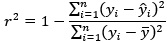
rather than as the square of the Pearson correlation coefficient. This ensures that negative correlations do not result in misleading positive R<sup>2</sup> values, as pointed out by the reviewer and discussed in Poldrack et al. (2020). All performance metrics (r, r<sup>2</sup>, MSE, and MAE) are now reported in Tables 1 and 2 to allow a more comprehensive and interpretable comparison of model performance.
We have included a description of the method under section 4.9. Statistical significance analysis.
(7) Could you clarify how data are standardized across training, validation, and tests (including Z-standardization for the cognitive tests)? This is to prevent data leakage.
Thanks for the comments. We did standardization the cognitive test from both training and test, separately.
We have added the following paragraph to the method section:
“A composite score of performances across the three tests was calculated and used as the measure of the cognitive domain in question (i.e., episodic memory, working memory). For each of the three tests, scores were summarized across the total number of trials. The three resulting sum scores were z-standardized and averaged to form one composite score for each domain. The standardization has been carried out independently for the training (DyNAMiC) and test (COBRA) samples.”
(8) There is really no ground truth to confirm that Grad-CAM provides actual feature importance used by the models. Perhaps the authors should compare that with Haufe transformation, which is commonly used in the predictive model for cognition (e.g., https://doi.org/10.1016/j.neuroimage.2021.118648 and https://doi.org/10.1016/j.neuroimage.2023.120115).
We appreciate the reviewer’s comment and the suggested references. The Haufe transformation is primarily applied in traditional machine learning models, particularly in cognitive neuroscience, to interpret linear predictive models by mapping classifier weights back to the input space. However, its direct applicability to deep learning models, especially convolutional neural networks, remains an open research area with no widely established methodologies. Furthermore, the Haufe transformation does not provide feature importance in the same manner as Grad-CAM. Grad-CAM highlights spatial regions within an image that contribute to a model’s decision, making it particularly useful for interpreting convolutional networks in vision tasks. In contrast, the Haufe method offers a weight transformation that is more suited for understanding linear models and may not be as intuitive for feature attribution in complex hierarchical representations such as those learned by deep neural networks.
While we acknowledge that Grad-CAM, like other interpretability methods, does not provide absolute ground truth validation for feature importance, it remains one of the most widely used and validated techniques for deep learning interpretability, particularly in medical imaging applications. Given its integration with frameworks such as Keras and TensorFlow and its ability to provide spatial attributions aligned with domain knowledge, we believe it is a suitable choice for our study. Future work may explore additional interpretability techniques, including adaptations of the Haufe transformation if applicable to deep learning architectures.
We have added more details on Grad-CAM implementations in the Method.
(9) Related to Grad-CAM, "These edges, indicated by a salience intensity of {greater than or equal to}.5, exert a significant influence on the model (Figure 1f)." What does 'significant' in this context mean? And how did the authors come up with the .5 threshold? Is it based on permutation or bootstrapping tests?
We appreciate the reviewer’s comment and the opportunity to clarify our approach. In this context, the term "significant" refers to the regions' relative contribution to the model’s decision, as shown by the Grad-CAM saliency map. However, to avoid implying statistical testing, we will revise the term to "highly contributing."
Regarding the 0.5 threshold, this value was selected empirically based on the normalized Grad-CAM activation values, where saliency scores range between 0 and 1. A threshold of 0.5 was used as a heuristic to highlight regions with relatively strong activation. However, this was not determined through statistical methods such as permutation or bootstrapping tests. We recognize the importance of rigorous threshold selection and will clarify this in the text. Future work could incorporate statistical methods to define thresholds more objectively.
We have included the following text in the Method section:
”Grad-CAM saliency maps were interpreted qualitatively, with a heuristic threshold (≥ 0.5) applied to highlight regions with relatively higher contribution to the model’s predictions. These values do not reflect statistical significance and should therefore be interpreted descriptively.”
(10) Still related to the saliency map, I believe the upper and lower triangles of the functional connectivity matrix are the same. If so, why are there some differences in saliency? While the difference is not prominent, this might affect the accuracy of Grad-CAM.
Minor differences in the saliency maps between the upper and lower triangles of the FC matrix can arise due to several factors. For instance, Grad-CAM generates saliency maps at the resolution of the convolutional feature maps, which are then upsampled to match the input matrix dimensions. We initially used the default bilinear interpolation, which may have introduced slight asymmetries or blurring, resulting in interpolation artifacts. In response, we have reprocessed the saliency maps using spline interpolation in MATLAB. The updated saliency figures have been included in the revised version of the manuscript.
(11) Why did the authors only report the cross-study for EM on rest, and for WM on n-back? This is a bit unexpected since COBRA has both rest and n-back. If there is no good justification, please report both.
We focused on reporting cross-study results for EM using rest because rest was the winning condition for predicting EM in the DyNAMiC sample. Importantly, n-back did not significantly predict EM in DyNAMiC, and rest did not significantly predict WM. For this reason, we highlighted only the conditions that showed meaningful predictive power in the original analyses.
(12) Are codes, trained models, and data available? To ensure transparency and reproducibility, I hope to see the code from preprocessing to modeling and statistical analyses.
The analysis code is openly available on our GitHub page https://github.com/MorEsm/AI-based-Prediction-of-Cognitive-Function. Due to ethical considerations and GDPR restrictions in the European Union, we are not permitted to publicly share the raw data. However, we can provide detailed information about preprocessing steps and analysis pipelines to facilitate reproducibility.
(13 &14) The authors did not appropriately control for regression-toward-the-mean and the influence of the working memory itself when calculating the brain cognition gap. This is commonly done to brain age (see https://doi.org/10.7554/eLife.87297.4, https://doi.org/10.1002/hbm.25533, https://doi.org/10.1016/j.nicl.2020.102229, https://doi.org/10.3389/fnagi.2018.00317). Otherwise, the brain cognition gap still depends on the cognition/working memory score itself. Based on Tetereva et al., "If, for instance, Brain Age was based on prediction models with poor performance and made a prediction that everyone was 50 years old, individual differences in Brain Age Gap would then depend solely on chronological age (i.e., 50 minus chronological age)." Because of this, Tetereva and colleagues found that the 'uncorrected' brain age gap that predicted chronological age the worst became the best index to predict fluid cognitive abilities. This shows the pitfall of the 'uncorrected' brain age gap. You can apply the same logic to the brain cognition gap.
(14) Additionally, another way to show the unique contribution of brain cognition, over and above cognition per se, is to add both brain cognition and cognition together to predict physical activity, education, and cardiovascular risk.
We thank the Reviewer for raising this important point. In response to their request and also the request from Rev. 1, we first examined the relationship between the Brain-Cognitive Gap (BCG) and the cognitive measure itself. Surprisingly, we did not find any significant relationship in either the DyNAMiC sample (r =0.01, p =0.939) or the COBRA sample (r =0.01, p =0.894) (see Author response image 1).
We then conducted additional analyses, splitting the sample into high and low EM performers, and compared their levels of physical activity and Framingham cardiovascular risk scores. We found that no significant difference in physical activity (DyNAMiC: p =0.56, CI: -14.99 – 8.13; COBRA: p =0.29, CI: -3.54 – 1.05) or Framingham CVD risk score (DyNAMiC: p =0.11, CI: -1.08 – 10.72; COBRA: p =0.41, CI: -1.86 – 4.58) between high and low EM perfprmers. Given the significant difference in physical activity and Framingham CVD risk score between positive and negative BCG groups, our results support that BCP provides unique information, beyond cognitive measure, regarding factors that contribute to cognitive resilience. These results have been added to Section 2.4, and Figure 3 has been updated.
(15) Related to the brain age gap, the brain cognition gap is actually just another way to quantify how generalizable models are to another sample, similar to MAE or MSE. If the models built from DyNAMiC don't fit well with samples from COBRA, you will get a higher (i.e., wider) brain cognition gap, which means a poor fit. The authors should discuss this interpretation - should your biomarker's performance be due to a fit of the model?
We appreciate this insightful comment. We agree that BCG can be interpreted not only as a marker of individual differences and resilience factors but also as a measure of model fit, analogous to error metrics, such as MAE or MSE. A higher gap may, in part, reflect poorer generalizability of models across samples. We have now revised the Discussion to explicitly acknowledge this alternative interpretation and to emphasize that BCG should be viewed both as a candidate biomarker and as a reflection of model performance.
We added the following paragraph in the discussion:
“An important caveat is that BCG can also be conceptualized as an error metric, similar to mean absolute error or mean square error, reflecting the extent to which models trained in one sample generalize to another. From this perspective, a larger gap may not only indicate individual differences related to resilience factors and dopaminergic function, but also reduced model fit or generalizability across datasets. Thus, BCG likely reflects a combination of meaningful biological variability and methodological variance.”
(16) It is unclear why the authors binarized the brain cognition gap when predicting physical activity, education, and cardiovascular risk, and not doing so with the striatal D1DR. It is rarely a good idea to binarize a continuous variable (see 10.1136/bmj.332.7549.1080). In this case, people who had a bigger negative brain cognition gap were treated equally to people who had a smaller negative brain cognition gap. I also do not think it is necessary to separately analyze positive and negative gaps. Perhaps the authors should correlate the corrected brain cognition gap with physical activity, education, and cardiovascular risk and provide scatter plots and effect sizes.
Following the reveiwer suggestion, we directly correlated BCG with physical activity and cardiovascular risk. Our results confirmed our initial analysis that individuals with a negative gap exhibited lower physical activity and higher Framingham CVD risk across both COBRA and DyNAMiC datasets. We have reported these results on page 10.
Author response image 5.
(17) Given that the motivation is to move away from brain age, the authors should benchmark the corrected brain cognition gap against the corrected brain age gap, as well as against the performance when directly predicting physical activity, education, and cardiovascular risk from the functional connectivity metrics.
Author response image 6.
We agree that benchmarking BCG against BAG in predicting lifestyle and vascular risk factors would be valuable. We have calculated adjusted BAG and related it to lifestyle and vascular risk factors. Interestingly, we did not find any significant association, suggesting that BCG might be more sensitive to cognitive resilience. However, this investigation was beyond the scope of the present study. Our aim was not to compare BCG with BAG, but rather to examine whether BCG provides information beyond cognition itself. We also note that introducing BAG would open a separate line of investigation, namely, which cognitive state (rest, movie-watching, n-back) best estimates biological age. While this is an interesting question in its own right, addressing it here would considerably broaden the scope and complexity of an already dense manuscript. To prevent misunderstanding, we have clarified this point in the Discussion and added a caveat noting that future work should explicitly benchmark these approaches. That said, if the Reviewer and/or the Editor incline to add these additional findings into the manuscript, we are open to doing so in a revision.
We have added the following sentence to the Discussion.
“While our focus was to investigate whether the brain–cognition gap provides information about factors contributing to cognitive resilience, we acknowledge that benchmarking BCG against the brain-age gap in predicting lifestyle and vascular risk factors would be valuable. However, addressing this question lies beyond the scope of the present study, and future work should systematically compare these approaches.”
(18) Why was only the working memory score used to create brain cognition, and not episodic memory as well? Including both could provide a more comprehensive measure.
We initially attempted to predict both episodic memory (EM) and working memory (WM). However, EM prediction was only reliable within and across samples for the resting state, whereas WM prediction generalized most strongly from the movie-watching condition. Because COBRA does not include a movie-watching paradigm, we could not evaluate WM prediction across datasets. For this reason, we focused on EM when examining the brain–cognition gap.
(19) The PET mediation analysis seemed to come out of the blue. Is there existing literature showing the relationship between striatal D1DR and cognition? If so, did the authors find a similar relationship in the current data? I also suggest rewriting this section to strengthen the justification for the PET mediation analysis.
We have previously conducted studies in which DA found to be associated with memory (Johansson et al., 2023, Nyberg et al., 2016).
The third aim of our study was to examine whether DA integrity is implicated in brain–cognition gaps (BCG), which we propose as a marker of cognitive resilience. In line with this aim, we found that lower DA receptor availability was associated with larger BCGs (Figure 4). We then asked whether this relationship is mediated by functional signal variability, such that lower DA is linked to reduced signal-to-noise ratio (i.e., greater entropy in functional connectivity), which in turn contributes to less reliable prediction of cognition and, consequently, larger BCGs. Our mediation analysis supports this pathway (see also our reply to Reviewer 1, Comment 6).
Thus, our mediation was not designed to test whether DA predicts episodic memory performance directly, nor whether BCG mediates such a relationship. Instead, we specifically investigated whether the effect of DA on BCG operates through functional variability. We agree that future work could extend our approach by directly examining whether BCG mediates the link between DA and cognitive outcomes. However, in the present study, our primary focus was on testing the mechanistic pathway of DA → entropy → BCG.
Minor recommendations:
(1) Task-based connections are not truly task-based, as they are around 70-80% related to the resting state, capturing non-task-specific functional connectivity. Task-based connections should refer to techniques that derive task-related connectivity, such as psychophysiological interaction and beta-series correlation. Perhaps use terms like "functional connectivity during tasks."
Thank you. This has been corrected throughout the manuscript.
(2) Are there really two studies? The same MRI was used with the same configurations, and participants were from the same city. The only difference is the age range. It may be more appropriate to refer to this as "across age groups" rather than "cross-datasets."
Thank you for this comment. While the two samples share some similarities, there are also several marked differences beyond age range. For example, Movie-watching was administered in DyNAMiC but not collected in COBRA. The resting-state fMRI sequence was 12 minutes in DyNAMiC but only 6 minutes in COBRA. Moreover, DyNAMiC included dopamine D1-receptor PET, whereas COBRA assessed dopamine D2-receptor availability. Even the questionnaires used to measure physical activity differed between the two studies. Given these methodological and measurement differences, we believe that referring to them as “cross-datasets” rather than “across age groups” more accurately captures the distinction.
(3) What kind of movie is "Cockpit"? Can you explain? Different movies may elicit different patterns of connectivity.
We apologize for not providing information about the movie, which has been presented in our recent work (Johansson et al., 2023).
The participants’ reactions to the content of the movie were not monitored, but the clips were selected to be as neutral in their content as possible. The content of the movie: Following his termination as a pilot and the end of his marriage, Valle embarks on a quest to secure new employment. Faced with desperation in the job market, he resorts to disguising himself as a woman with the intention of obtaining a position at a company specially seeking a female pilot.
This information is added to the method section.
“During the fMRI session, participants viewed a 12-minute segment from the Swedish comedy film Cockpit (2012). We did not monitor participants’ responses to the movie, and the chosen clips were selected to be relatively neutral in emotional content. The storyline follows Valle, a recently fired pilot whose marriage has ended, as he struggles to find new employment. In a desperate attempt to secure a job at an airline specifically recruiting a female pilot, he presents himself as a woman.”
(4) There is a typo in the equation numbering (i.e., two equations are designated as #1).
We have now corrected the typo.
(5) From the discussion: "Importantly, this prediction generalizes across conditions." This is not surprising given the similarity between conditions, with around 70-80% variance.
We agree with the reviewer that the high similarity of FC across states likely increases the chance of cross-condition generalizability. However, this generalization is not guaranteed for all models. For example, the model trained on FC during movie-watching successfully predicted episodic memory during rest, but it did not generalize to episodic memory during the n-back condition, although movie-watching and n-back FC patterns are themselves highly correlated. Thus, the observed generalization is meaningful in demonstrating that not all models transfer equally well across states.
That said, we have added the following sentence to the Discussion:
“Importantly, this prediction generalizes across conditions and datasets, suggesting that features derived from resting state FC serve as a relatively stable marker of individual differences in EM, though with reduced strength in COBRA. While such generalization is partly facilitated by the similarity of functional connectivity across states, it is not a trivial outcome. For instance, the model trained on movie-watching data generalized to EM prediction during rest but failed to do so for the n-back condition, even though movie-watching and n-back connectivity patterns are themselves highly correlated. This indicates that successful generalization depends not only on shared variance across states but also on the cognitive processes most relevant to the target behavior.”
(6) It might be helpful to include some figures for the cognitive tasks used. The description is a bit hard to follow without visual aids.
Thanks for the comment. We have had a figure describing this in the initial paper about DyNAMiC (Nordin et al., 2022). We have added the Supplementary Figure (Fig S3) in the manuscript.
Fig S3. Overview of the cognitive tests included in the DyNAMiC study. Adopted from Nordin et al. with permission.
(7) It may not be appropriate to use the term "cross-validation" here, as one dataset was used for testing and the other for training, but not vice versa (so no "cross" per se).
We thank the reviewer for pointing this out. We agree that the term “cross-validation” is not precise in this context, since we trained the model in one dataset and tested it in another without performing the reverse. We have revised the manuscript to use the term “external validation” instead of “cross-validation” to more accurately describe our cross-dataset approach.
(8) I don't have access to the supplementary materials or code/data, so all of the comments here are based on the main text.
We have added the supplementary materials and inserted the GitHub link to the code.<br />
Reviewer #3 (Recommendations for the authors):
I suggest benchmarking against other simpler algorithms and controlling for memory in the brain cognition gap analyses.
The authors might also want to simplify some aspects of the paper. There is a lot going on, which leaves less space to go into enough details for some analyses to warrant claims in the discussion. For example, the authors only compare the deep net to CPM and kernel ridge based on the literature. Direct comparisons would be needed.
Thanks for the comment. We have made an attempt to address the concerns outlined in the public recommendation. Our study explicitly compares predictive power across different cognitive states (rest, movie watching, n-back), with the aim of identifying the states that best capture individual differences across domains. Thus, our goal was not to propose a universally superior prediction model, but rather to test how brain state influences predictive utility for WM and EM using a deep learning approach. We have revised the manuscript text to make this focus clearer and to avoid any misinterpretation of our aims. Specifically, we removed statements in the Discussion that could be read as suggesting that our deep learning approach outperforms prior machine learning methods. While we compared our model with the connectome predictive modeling (CPM) approach and observed better performance with our deep learning framework, we did not conduct a comprehensive benchmark across all available machine learning methods, nor was this the aim of the present study. Accordingly, we have adjusted the text to avoid implying methodological superiority beyond the scope of our analyses. Furthermore, we have controlled for memory as suggested by the reviewer and outlined in response to reviewer 1.