Author response:
The following is the authors’ response to the original reviews
Reviewer #1 (Public review):
We truly appreciate all the effort that the reviewer put into reading and understanding our work. With a total of 37 excellent questions, this is one of the most thorough reviews that we have received in a long time.
R1.0: Summary:
In this study, the authors propose a "unifying method to evaluate inter-areal interactions in different types of neuronal recordings, timescales, and species". The method consists of computing the variance explained by a linear decoder that attempts to predict individual neural responses (firing rates) in one area based on neural responses in another area.
The authors apply the method to previously published calcium imaging data from layer 4 and layers 2/3 of 4 mice over 7 days, and simultaneously recorded Utah array spiking data from areas V1 and V4 of 1 monkey over 5 days of recording. They report distributions over "variance explained" numbers for several combinations: from mouse V1 L4 to mouse V1 L2/3, from L2/3 to L4, from monkey V1 to monkey V4, and from V4 to V1. For their monkey data, they also report the corresponding results for different temporal shifts. Overall, they find the expected results: responses in each of the two neural populations are predictive of responses in the other, more so when the stimulus is not controlled than when it is, and with sometimes different results for different stimulus classes (e.g., gratings vs. natural images).
Strengths:
(1) Use of existing data.
(2) Addresses an interesting question.
R1.1: Unfortunately, the method falls short of the state of the art: both generalized linear models (GLMs), which have been used in similar contexts for at least 20 years (see the many papers, both theoretical and applied to neural population data, by e.g. Simoncelli, Paninsky, Pillow, Schwartz, and many colleagues dating back to 2004), and the extension of Granger causality to point processes (e.g. Kim et al. PLoS CB 2011). Both approaches are substantially superior to what is proposed in the manuscript, since they enforce non-negativity for spike rates (the importance of which can be seen in Figure 2AB), and do not require unnecessary coarse-graining of the data by binning spikes (the 200 ms time bins are very long compared to the time scale on which communication between closely connected neuronal populations within an area, or between related areas, takes place).
First, a few points of clarification.
(i) We worked with two-photon calcium imaging data (mice), and with the envelope of multi-unit activity (monkeys). While both of these types of signals are strongly correlated with spikes, neither of them can be truly considered to be a point process.
(ii)The reviewer points to Figure 2AB. The signals that we worked with can be negative. The black traces are the actual signals and show clear negative bouts, especially noticeable in the middle panel in Figure 2B. Of course, this does not mean that there are negative spike rates. This has to do with the way the data are normalized and not with the specific prediction method. However, the reviewer is correct in stating that the method that we used could also yield negative values even for non-negative spike rates.
(iii) We did not bin the macaque data into 200-ms time bins, but rather 25-ms time bins (line 548, Figure 1B legend). Additionally, we have now performed additional analyses with different window sizes, showing that the conclusions still hold (see Supplemental Figure 4 and lines 139-143).
To further address the reviewer’s question, we implemented a Poisson GLM enforcing non-negativity on macaque MUAe data (without spontaneous activity subtraction, ensuring strictly positive values; lines 135-139, Supplemental Figure 1M). The model did not improve predictions over ridge regression, confirming our methodological choice. This method is not directly applicable to mouse calcium data, since the activity after baseline subtraction can be negative.
We did not use Granger or any other causality methods. The question of causality is certainly important, and there are multiple methods developed to assess causality in neural signals. We do not make any claims about causality in our study. A rigorous evaluation of causality is an interesting line of research for future work.
R1.2: In terms of analysis results, the work in the manuscript presents some expected and some less expected results. However, because the monkey data are based on only one monkey (misleadingly, the manuscript consistently uses the plural ‘monkeys’), none of the results specific to that monkey, nor the comparison of that one monkey to mice, are supported by robust data.
We have now added data from 2 additional monkeys, including:
(i) A second monkey (monkey “A”) from the same dataset (Chen et al., 2020), which includes all activity types except the lights off condition (lines 90-96, 120-132, 159, 161, 171, 183-185, 188-194, 200-203, 228-237, 254-258, 292-296, 334-342, 351-353, 358-364, 374-378, 387-393, 400-408, 414, 417-421, 539-540, 544-545, 680-681, 696-698; Supplemental figures 1-6, 8, 11, 12, and 13; Table 2).
(i) We collected new neural activity from one additional monkey (monkey “D”) in collaboration with the Ponce lab (lines 90-96, 120-130, 132-134, 163-164, 228-235, 237-243, 292-296, 351-353, 374-378, 387-389, 539-540, 553-560, 696-698; Supplemental figures 1-2, 4, 6, 9, 11, and 12; Table 2). The new data include responses to the same checkerboard and gray screen images as the original dataset, along with responses during lights-off conditions.
R1.3: One of the main results for mice (bimodality of explained variance values, mentioned in the abstract) does not appear to be quantified or supported by a statistical test.
We have now formally quantified the bimodality of the relationship between one-vs-rest correlation and inter-laminar explained variance (EV) in mice using Hartigan’s dip test, applied to neurons with EV>0.4. The test confirmed significant bimodality in two of the three mice (MP031 and MP032: p<0.001; MP033: p=0.687). These results are now included in the Results section (lines 307-311) and shown in Supplemental Figure 7A,D. In datasets that did not show bimodality by visual inspection (macaque recordings), the same test yielded non-significant results (e.g., p=0.994), confirming that the statistical analysis distinguishes between bimodal and unimodal cases.
R1.4: Moreover, the two data sets differ in too many aspects to allow for any conclusions about whether the comparisons reflect differences in species (mouse vs. monkey), anatomy (L2/3-L4 vs. V1-V4), or recording technique (calcium imaging vs. extracellular spiking).
We also agree with this comment. Our goal is not to provide any direct quantitative comparison between the two species. We emphasize (lines 494-497) that the experiments in the two species differ along multiple dimensions, including: (i) differences in recording modalities (calcium vs. electrophysiology), (ii) associated differences in temporal resolution, neuronal types, and SNR, (iii) cortical targets (layers vs. areas), (iii) sample size, (iv) stimuli, (v) task conditions. In the revised manuscript, we also emphasized that the aim of this work is to investigate inter-areal interactions within each species rather than to draw quantitative comparisons between species (lines 497-499).
Reviewer #1 (Recommendations for the authors):
R1.5 In the analysis of directionality, you stated that subsampling was done randomly. Presumably, there could be multiple subsamples that fulfill the control of split-trial r. Are you only showing results from one subsample or multiple subsamples?
We show the median from 10 subsample permutations. This is now clarified in line 621.
R1.6 About the measurement 1-vs-rest r2. Understanding the definition is important for interpreting the results, but the definition was not clearly written. In lines 195-196, could you be more clear about whether the correlation is between the predicted neuron and other neurons in the predicted population or between the predicted neuron and the mean activity of the predictor population? Also, in line 212, why do you call this self-consistency? Isn't this a correlation between a neuron and the others?
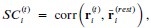
The 1-vs-rest r<sup>2</sup> value, or self-consistency, is the correlation calculated for each neuron i and does not involve other neurons. Let  indicate the response 𝑟 of neuron i during trial t (t=1,..., T where T is the total number of trials). For a given trial t, we compute the average activity of the neuron excluding this trial:
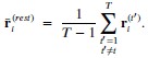
Throughout, the superscript (rest)means “all repetitions excluding repeat 𝑡”. The one-vs-rest correlation for the held-out repetition 𝑡 is:
We then average these correlations across all held-out repetitions:
We now clarify this in the text (lines 304-306 and lines 642-647).
R1.7 In Figure 6 G and I. The "all" condition contains more neurons than either of the other two. In this case, is this comparison fair or meaningful?
The reviewer is also correct here. The comparisons between the <10% and >80% groups contain the same number of predictor neurons, and those are fair comparisons. The “all” condition contains more predictor neurons, and, therefore, those comparisons are not fair. We clarified this point in lines 360-364.
We included the “all” condition here because we think that it is an instructive sanity check in terms of reporting how EV changes with more neurons, and also in terms of understanding why the EV values in the other two conditions are lower. Expanding on this point with a little bit of philosophy, ultimately, when considering a neuron in area B (e.g., V4) and the contributions from neurons in another area A (e.g., V1), one would like to have access to all the inputs (e.g., all the neurons in V1 that are monosynaptically connected to the target neuron in area V4). We do not have access to this type of information, and we do not make any claims about monosynaptic connectivity, let alone exhaustive sampling of inputs to a given neuron. The “all” condition merely provides a quantitative illustration of the fact that EV increases with the number of predictor neurons. This observation may be considered to be somewhat trivial, but it should be pointed out that the conclusion relies on the input neurons sharing information with the target neurons (e.g., perhaps one may not be able to predict V4 activity very well from the responses of millions of neurons in the cerebellum).
R1.8 I believe the results section can be improved by adding some interpretation after each finding.
We thank the reviewer for the suggestion. We generally like to separate results from interpretation. However, to honor the suggestion, we added brief interpretations throughout the results section (lines 142-143, 171-173, 272-273, 279-281, 331-333, and 361-364) and expanded on the interpretations in the Discussion section.
R1.9 Line 52 - 74: It would be better to be more specific about what kind of neuronal interactions, e.g., noise correlation, synchrony, etc.
We added a clarification on the types of interactions we study in lines 68-73.
R1.10 Line 81. Something seems to be missing after "5500". 5500 trials? Neurons?
We thank the reviewer for pointing this out. The number refers to neurons (fixed in line 87).
R1.11 Line 94. The readers would appreciate more explanation of the method.
We have expanded on the explanation, as suggested (lines 106-107).
R1.12 Line 104. The fraction of visually responsive neurons seems to be small. Is this typically for mouse V1? Would this fraction be higher if you also used the peak, as you did for macaque data in your SNR calculation (line 412)? And what is this number for the recorded L4?
The reviewer correctly points out the small number of visually responsive neurons.
We note that we now refer to the subset of neurons used for prediction analyses as visually reliable (VR) neurons (lines 115-116, 125-126, 178-179, 183-184, 211-212, 214-216, 217-226, 283-286), defined conservatively as neurons with SNR > 2 computed from the mean across all stimuli (not the peak to any one stimulus) and split-half reliability >0.8 (Methods, lines 569–590). This choice emphasizes neurons that are consistently informative over the full stimulus set.
Regarding the question of how typical the number of responsive neurons in mice is, the fraction of “responsive” neurons in mouse V1 varies widely depending on the definition and stimulus set but the fractions are substantially lower than those reported in monkeys (with different methods). For those of us more used to the macaque neurophysiology literature, this has been one of the biggest surprises coming from work in rodents. Many studies report a sizable group of non-responsive neurons in mouse V1 (e.g., as little as 37% percent of V1 neurons being responsive in at least 25% of the trials according to de Vries et al., Nat Neur, 2020). Our fraction of visually responsive neurons is small because it couples a conservative SNR metric with a high trial-reliability threshold.
As the reviewer notes, a peak-based metric based on any stimulus would be a less conservative criterion that would increase the fraction of neurons labeled responsive.
R1.13 Line 113. Why not also give an exact percentage number?
We have given the exact percentage number (lines 125-126).
R1.14 Line 128. Is this just because L2/3 has more neurons? If so, then isn't this trivial?
Our intention was to illustrate the best prediction performance we could get in either direction, which means including all L2/3 neurons. We have reworded our text to clarify (lines 149-151).
R1.15 Line 134. Isn't this expected? Since V1 have more units than V4?
The reviewer is correct. As discussed in R1.7 in mice, we sought to report the best prediction performances in either direction. We have edited our text for clarity (lines 149-151).
R1.16 Line 165-168. What's the logical connection between these two sentences? If the former is true, we should expect to see differences. Also, why the same population? Shouldn't you include non-visual neurons?
The two sentences in question are: “The difference in predictability in the absence of a stimulus could in principle change according to the directionality in inter-laminar interactions.” and, “There was no statistically significant difference in the EV fraction between laminar directions (L4→L2/3 vs. L2/3→L4) using the same control population as in Figure 3B (Figure 5A-C and Figure Supplement 2H).”. The key point here was to control for similar reliability values in order to make fair comparisons. We have added an additional comparison between directionalities focusing on nonvisual neurons (SNR<2 & r<0.8), and have also found no statistically significant difference between direction of predictability (Supplemental Figure 3A, right, lines 221-224).
R1.17 Table 2. The information of which session corresponds to which experiment can be put in the table, which would be easier to read.
We have added which sessions correspond to which experiments in Table 2.
R1.18 Figure 1, Captions for panel c and d. I don't see any colored arrows in the figure.
We removed the color descriptions (Figure 1C-D).
R1.19 Figures 3, 4, and others. The annotations of "n.s." are very hard to see.
We changed the color so that it is easier to see now (Figures 3, 4, 6, and Supplementary Figures 1-4, 6, and 8-10).
R1.20 Figure 5, panel A. The legend is too small.
We increased the legend size (Figure 5A).
R1.21 Figure S5, panel D. Why are some of the data points connected?
The paired connections are illustrated specifically in the highly predictable neurons to highlight the two separate distributions of neurons. One group, the highly predictable and highly reliable group, maintains its inter-laminar predictability after projecting out the “non-visual” activity (lines 327-330), whereas the highly predictable yet unreliable group shows a sharp decrease in inter-areal predictability, which corroborates the idea of non-visual components influencing neurons in mouse V1, as shown by Stringer et al. 2019b and consistent with our results.
R1.22 l.91 "Ope" -> open?
We fixed the typo (line 100).
R1.23 Fig. 3C+D: Why is only one session used for this?
One session was used to illustrate the distribution of split-half reliability values per area. Figure 3D contains information about all 5 stimulus sessions (see legend to Figure 3D).
R1.24 "Even without controlling for the number of predictors or their respective split-half correlation values (627-688 sites in V1, 86-115 sites in V4), we found better predictability in the V1 to V4 direction than the reverse ( 𝑝 < 0.001, Figure Supplement 2I)." -> What does "even" mean here? Isn't this simply the null result if there is no true difference and the real reason the authors controlled for size?
The reviewer’s understanding is correct. We have edited our text for clarity (lines 157-160)
R1.25 "We could predict V1 and V4 activity across all stimulus types ( 𝑝 < 0.001, paired permutation test of prediction vs. shuffled frames prediction)." -> better than chance? For all neurons on average? What does this mean? Isn't it trivial and 100% expected that neural activity in the visual cortex is above chance related to the visual input?
We stated that sites in V1 and V4 could predict each other across all stimulus types before describing the differences between them. We agree that this observation is to be expected and indicated so now in the text (lines 185-186).
R1.26 "The predictability was the highest in both directions for neuronal activity in response to a full field checkerboard images (Figure 4D). In the V1 → V4 direction, the EV fraction was higher when predicting a slow-moving small thin bar compared to a fast-moving large thick bar (Figure 4D, left), whereas the opposite was true for the V4 → V1 direction (Figure 4D, right)." -> What does this mean? Is this expected or not? Under what theories of cortical processing?
The differences between EV prediction directions (V1→V4: slow thin bars > fast thick bars; V4→V1: fast thick bars > slow thin bars) could be because V4 responses are more reliable for the slow thin bars whereas V1 responses are more reliable for the fast thick bars (Supplemental Figure 5H–I). To account for this possibility, we controlled for differences in target-related properties by regressing out covariates like SNR, split-half correlation, and variance. In monkey L, regressing out reliability/drive within direction using these covariates, the V4→V1 bar difference between slow thin bars and fast thick bars was not significant and the difference in the V1→V4 difference direction was reduced (Supplemental Figure 5K, lines 198-203). This suggests that the asymmetry primarily reflects stimulus‑dependent reliability of the target population rather than a strong directional selectivity.
To the best of our knowledge, there are no clear predictions that match these observations from existing theories of visual cortical processing, especially given the paucity of computational models that include stimulus velocity when describing the responses in area V4. There has been extensive work on theories of surround suppression, but it seems unlikely that the thick bars would elicit surround suppression given the size of the V4 receptive fields. Many current computational models that aim to fit the responses of neurons in the visual cortex use neural networks that take an image as visual input and yield activations. Most of these models do not incorporate stimulus movement, and even those that do incorporate stimulus dynamics, only indirectly map onto interlaminar stimulus transformations or even between-area stimulus transformations. We hope that the results in this manuscript will help inspire and constrain better models of visual cortical processing.
R1.27 Shouldn't all the predictability analysis be done conditioned on the stimulus in order to tell us more than the trivial "both V1 and V3, or L2/3 and L4, are driven by visual inputs"? (The spontaneous activity analyses are essentially that, for a small subset of the stimuli.)
The key goal of this study is to quantify inter-areal interactions both under visual input and without visual input. This type of analysis is important because inter-areal interactions may depend both on visual inputs but also on neuronal inputs that are not triggered by visual signals. For example, extensive work in mice has now shown that neuronal responses in V1 depend on an animal’s running speed, independently of any visual input. Even within the visual input conditions, we present analyses where we shuffle trial order (e.g., Figure 7, Supplementary Figure 11) to estimate the contribution of trial-by-trial variations that are independent of visual inputs and other analyses where we project out non-visual activity (e.g., Supplementary Figure 7).
R1.28 "In visually responsive neurons, there was a significant reduction in EV during gray screen compared to visual stimulus presentation" -> perfectly expected. But the report-worthy result here is how much is left, not whether EV is decreased!
We have changed the wording on the results to highlight the sustained predictability (lines 211-212). It is important to note that, although the reduction in EV during gray screen may be expected, this observation does not hold for all neurons. In fact, there are some neurons for which the EV during visual presentation is comparable to that during gray screen (Figure 5B,C,E: neurons that lie on the diagonal line).
R1.29 "Similar to the conclusions drawn from the mouse data, the predictability of neuronal activity was higher in response to stimulus presentation than to gray screen presentations" -> Really? Conditioned on stimulus, or explainable by the well-known fact that both V1 and V4 are visually driven?
As discussed in R1.28, in mice, there are many neurons where the EV during gray screen is comparable to that during stimulus presentation. In monkeys, most sites were visually driven. As the reviewer points out, we expected that EV during stimulus presentation would be higher than during gray screen; this observation is a reasonable sanity check. The difference between unshuffled trials and shuffled trials (Figure 7, Supplementary Figure 11) provides an estimate of the interactions that are not purely explained by visual inputs alone in monkeys.
R1.30 "Unlike the mouse, macaque correlation of visual predictability between stimulus presentation and spontaneous activity was high across all types of spontaneous conditions" -> Why? Is this simply explainable by a lower mean response in the spontaneous condition in the mouse? Are these mouse and monkey experiments truly comparable? Isn't it surprising that spontaneous activity in the monkey visual cortex compared to evoked activity is higher than in the mouse?
With respect to the question of whether spontaneous activity (or stimulus-evoked activity) in monkeys is higher than in the mouse, it is difficult to make these comparisons. We emphasize in the text the multiple differences between the experiments in both species. Our goal is not to perform any quantitative comparison across species (see R1.4). We changed the wording to remove any inference of comparison between species (lines 248-250).
R1.31 Occasionally imprecise presentation. Ex "To further examine the non-stimulus driven component, we reasoned that if the shared information between areas were strictly driven by the visual stimulus, then using the activity of a stimulus presentation repeat to one specific image could be used to predict the responses to any other stimulus repeat of the same image. On the other hand, if the shared activity does not have any stimulus-response information, then the prediction model would not work when considering responses across repeated presentations of identical stimuli in different trials. To test these two opposing ideas, we compared the inter-areal prediction EV fractions using unshuffled versus shuffled trials." -> Sets up two extreme strawmen (100% driven by stimulus vs 0% driven by stimulus). What does "model would not work" mean? EV=0? Hypotheses not ideas.
Our intent was to set up two extreme hypotheses, not to claim that neurons must fall exclusively into one or the other. The two extremes help better interpret the results.
The reviewer indicates that these are straw-man hypotheses. This may well be the case. But note the responses to R1.12, R1.27, R1.28, and R1.29. The reviewer seems to assume that all or most neurons in the visual cortex should be mostly or exclusively driven by visual stimuli.
We also replaced “ideas” with “hypotheses”, as suggested. We have expanded the discussion of these points in the manuscript (lines 480-493). Many neurons occupy intermediate positions between these two extreme hypotheses. We clarified that “model would not work” refers to prediction accuracy approaching chance (EV ≈ 0).
R1.32 "In both species and in both directions, inter-areal prediction EV fraction persisted (𝑝 < 0.001," Doesn't persist mean EV is unchanged? But the test is EV>0 or not in both cases.
We meant that EV values remained significantly above chance, not that they were unchanged. The statistical test was indeed whether EV > 0 as the reviewer indicated. We have revised the text accordingly (lines 375-380).
R1.33 "In mice, neurons showed a bimodal distribution in terms of their response predictability in shuffled and unshuffled trials" -> I don't see any bimodality in the figure, nor is there a statistical test provided for bimodality.
In Figure 7C, a group of neurons lay essentially along the horizontal axis, whereas the other group is dispersed closer to the diagonal line. Specifically, the neurons that lay on the horizontal axis are also the ones whose responses are best predicted during gray screen activity. We have changed the text to clarify this point (lines 380-382).
R1.34 "In the macaque V4 → V1 direction, there was a large proportion of neurons with peak EV when considering 25 ms to 50 ms offsets in the positive direction (i.e., V4 after V1, Figure 7I, right)." -> So what does this mean? Is this compatible with anything we know? This is the anti-causal direction so some kind of explanation would be warranted.
In the V4→V1 panel, a positive offset means we use V4 at t+Δt to predict V1 at t (and conversely in the V1→V4 panel). Therefore, the fact that the peak EV occurs at +10–20 ms indicates that V1 leads V4 by ~10–20 ms: in other words, V1’s earlier response best predicts V4’s slightly later response. This observation is not anti-causal, but rather it is consistent with the canonical largely feed-forward V1→V4 latency (e.g., Schmolesky et al., 1998 among many others). We clarified this in text (lines 400-404).
R1.35 L. 307: "In monkeys," plural!?
While this was not correct in the original version, we have now added data from two more monkeys.
R1.36 L. 313: "we observed an approximately bimodal distribution of neuronal responses, with a large subset of neurons that do not show reliable responses to visual stimuli both in L4 and L2/3" -> where?
The bimodal distribution can be appreciated in Figure 6B (1-vs-rest r2, third panel, note neurons along the y-axis, see also R1.33) and Supplementary Figure 7B (lines 307-312). Additionally, as stated in R1.3, we have now formally quantified the bimodality of the relationship between one-vs-rest correlation and inter-laminar explained variance (EV) in mice using Hartigan’s dip test (lines 310-313); see also Supplementary Figure 7A,D. In datasets that did not show bimodality by visual inspection (macaque recordings) the same test yielded non-significant results, confirming that the statistical analysis distinguishes between bimodal and unimodal cases.
R1.37 Random subsampling to control for population size done with how many subsamples? How are they combined? Variability across subsamples interpreted how?
We performed 10 permutations and used the median distributions across permutations (line 621).
Reviewer #2 (Public Review):
R2.0: “Summary:
In this work, the authors investigated the extent of shared variability in cortical population activity in the visual cortex in mice and macaques under conditions of spontaneous activity and visual stimulation. They argue that by studying the average response to repeated presentations of sensory stimuli, investigators are discounting the contribution of variable population responses that can have a significant impact at the single trial level. They hypothesized that, because these fluctuations are to some degree shared across cortical populations depending on the sources of these fluctuations and the relative connectivity between cortical populations within a network, one should be able to predict the response in one cortical population given the response of another cortical population on a single trial, and the degree of predictability should vary with factors such as retinotopic overlap, visual stimulation, and the directionality of canonical cortical circuits.”
R2.1: To test this, the authors analyzed previously collected and publicly available datasets. These include calcium imaging of the primary visual cortex in mice and electrophysiology recordings in V1 and V4 of macaques under different conditions of visual stimulation. The strength of this data is that it includes simultaneous recordings of hundreds of neurons across cortical layers or areas. However, the weaknesses of calcium dynamics (which has lower temporal resolution and misses some non-linear dynamics in cortical activity) and multi-unit envelope activity (which reflects fluctuations in population activity rather than the variance in individual unit spike trains), underestimate the variability of individual neurons. The authors deploy a regression model that is appropriate for addressing their hypothesis, and their analytic approach appears rigorous and well-controlled.
We agree with these points, and we discuss these specific limitations in capturing the variability of individual neurons in the Discussion section (lines 500-504). We have now also added analyses based on local field potentials (LFP). LFPs do not directly reflect the activity of individual neurons either.
R2.2: From their analysis, they found that there was significant predictability of activity between layer II/III and layer IV responses in mice and V1 and V4 activity in macaques, although the specific degree of predictability varied somewhat with the condition of the comparison with some minor differences between the datasets. The authors deployed a variety of analytic controls and explored a variety of comparisons that are both appropriate and convincing that there is a significant degree of predictability in population responses at the single trial level consistent with their hypothesis. This demonstrates that a significant fraction of cortical responses to stimuli is not due solely to the feedforward response to sensory input, and if we are to understand the computations that take place in the cortex, we must also understand how sensory responses interact with other sources of activity in cortical networks. However, the source of these predictive signals and their impact on function is only explored in a limited fashion, largely due to limitations in the datasets. Overall, this work highlights that, beyond the traditionally studied average evoked responses considered in systems neuroscience, there is a significant contribution of shared variability in cortical populations that may contextualize sensory representations depending on a host of factors that may be independent of the sensory signals being studied.
We agree that these datasets do not lend themselves well to directly separating and quantifying all the different sources of the predictive signals. We expand on this point in the Discussion section (lines 509-511).
R2.3: The different recording modalities and comparisons (within vs. across cortical areas) limit the interpretability of the inter-species comparisons.
We also agree with this comment. We emphasize that our goal is not to attempt a direct quantitative comparison across species (lines 497-499).
R2.4: Strengths:
This work considers a variety of conditions that may influence the relative predictability between cortical populations, including receptive field overlap, latency that may reflect feed-forward or feedback delays, and stimulus type and sensory condition. Their analytic approach is well-designed and statistically rigorous. They acknowledge the limitations of the data and do not over-interpret their findings.
Weaknesses:
The different recording modalities and comparisons (within vs. across cortical areas) limit the interpretability of the inter-species comparisons.The mechanistic contribution of known sources or correlates of shared variability (eye movements, pupil fluctuations, locomotion, whisking behaviors) were not considered, and these could be driving or a reflection of much of the predictability observed and explain differences in spontaneous and visual activity predictions.
We have expanded on the Discussion section to explicitly state the points raised by the reviewer (lines 494-509).
In mice, we have now also analyzed a separate dataset in which behavioral measurements were available, including running speed and facial motion (FaceMap SVDs). We used these to build behavioral-only and combined models to predict neural activity. We found that behavioral variables explained a modest but consistent portion of the variance across both spontaneous and stimulus conditions (Supplementary Figure 10A,C, lines 268-273).
For the macaque data, we analyzed pupil size as the only available behavioral measure in the macaque dataset. We focused specifically on the “resting state, eyes open” condition, where both neural activity and pupil measurements were available. Using ridge regression, we assessed the extent to which pupil size predicted neural activity in V1 and V4. Pupil size alone explained only a small fraction of the variance (Supplementary Figure 10E, lines 274-276).
R2.5: Previous work has explored correlations in activity between areas on various timescales, but this work only considered a narrow scope of timescales.
Without going into specifics about the numbers, it is hard to fully address this question. As the reviewer noted in R2.1, the mouse data analyzed here do not lend themselves to evaluating predictability on scales of tens of milliseconds. In the macaque data, we have now conducted additional analyses where we binned the activity across a range of bin sizes (10 ms to 200 ms). The new analyses are shown in Supplementary Figure 4, and described in lines 140-143, 160-163.
R2.6: The observation that there is some degree of predictability is not surprising, and it is unclear whether changes in observed predictability with analysis conditions are informative of a particular mechanism or just due to differences in the variance of activity under those conditions. Some of these issues could be addressed with further analysis, but some may be due to limitations in the experimental scope of the datasets and would require new experiments to resolve.
First, we note that several of the analyses and comparisons are within conditions and not across conditions, where by “condition” we mean the presence or absence of a stimulus or different stimuli (e.g., Figures 3, 5, 6, 7, Supplementary Figures 3-4, 7–13).
Second, we note that our mouse preprocessing standardized responses by spontaneous mean and SD per neuron, controlling baseline scale across conditions (lines 535-538). Because of this standardization, spontaneous traces have unit scale (mean = 0, SD = 1).
To test whether differences in variance underlie our findings, we calculated the variance for both species. For mice, we computed variance across repeats (visual) and across timepoints (lines 286-291). For the macaque moving-bar sessions, we computed variance across the concatenated held-out samples pooling timepoints, repeats, and bar identities (lines 291-292).
The V4 population showed a higher overall variance distribution compared to the V1 population (Supplementary Figure 2I-J), and L2/3 variance was also overall higher than L4 (Supplementary Figure 2D-E). We also see a modest monotonic relationship between EV fraction and this variance (mouse visual: Spearman ρ = 0.43–0.52, p < 0.001; macaque stimulus responses: ρ = 0.50–0.56, p < 0.001; macaque gray-screen responses: ρ = 0.38, p < 0.001, Figure 6A,D), indicating variance contributes to (but is not the primary driver of) EV prediction fraction. We then adjusted for variance by fitting, within each stimulus condition, a linear regression of EV on variance (excluding shuffled-control rows) and conducted all comparisons on the resulting residual EV values, thereby isolating effects not attributable to variance (see Supplementary Figure 3E-G, lines 165-171).
Reviewer #2 (Recommendations for the authors):
R2.7 Overall I found this manuscript to be very clearly written and the results compelling, although I found myself wanting a little more. I believe these datasets also include information about eye movements, pupil diameter, and maybe locomotion and whisking in the rodent work. I think it could be informative to ask the degree to which the predictability, particularly during the spontaneous activity, is attributable to these other known sources of variance in trial-by-trial measures. My concern is that during visual stimulation, the space of cortical responses is limited to a very narrow scope (observing a visual stimulus during fixation) whereas spontaneous activity includes a broader range of possibilities (different states of arousal, eye movement).
We analyzed the role of behavioral variables that could explain the neural activity in mouse V1 (including the variables suggested by the reviewer, running speed, facemap SVDs). The open dataset authors warned not to use pupil size since in the dark, the measurements were not accurate. In terms of the contribution to the predictability of mouse V1 activity, these behavioral variables showed a weak yet significant contribution (Supplementary Figure 10A,C, lines 260-270).
R2.8 By controlling for eye movements or pupil diameter during spontaneous measurements, would you improve your measure of predictability?
When predicting neural activity in the lights-off eyes open condition, combining neural data of the predictor population with information of pupil size did not result in a statistically significant increase in EV fraction when predicting the target population (Supplementary Figure 10E, lines 276-278).
R2.9 Also, there is work that shows feed-forward correlations between V1 and higher visual areas are observed in higher frequency activity, whereas feedback is associated with lower frequency activity. If you compared your predictability measure over bandpasses with different timescales, would you find the direction of V1-V4 interactions changes consistent with this previous work?
To address this question, we extended our analyses to the local field potential signals (LFPs) in monkeys, using band-limited LFP power (2–12, 12–30, 30–45, 55–95 Hz). We reran the lag sweep analyses (10-ms steps; 200-ms windows slid every 10 ms) in both directions. The Gamma band showed a feed-forward signature in the early evoked period: the V1→V4 predictability peaked at negative offsets (∼10–30ms; V1 leads), and the V4→V1 predictability peaked at positive offsets, consistent with previous findings. The results for low and beta frequency bands are also presented in the text (Supplemental Figure 13, lines 412-423).
Reviewer #3 (Public review):
R3.0: Neural activity in the visual cortex has primarily been studied in terms of responses to external visual stimuli. While the noisiness of inputs to a visual area is known to also influence visual responses, the contribution of this noisy component to overall visual responses has not been well characterized.
In this study, the authors reanalyze two previously published datasets - a Ca++ imaging study from mouse V1 and a large-scale electrophysiological study from monkey V1-V4. Using regression models, they examine how neural activity in one layer (in mice) or one cortical area (in monkeys) predicts activity in another layer or area. Their main finding is that significant predictions are possible even in the absence of visual input, highlighting the influence of non-stimulus-related downstream activity on neural responses. These findings can inform future modeling work of neural responses in the visual cortex to account for such non-visual influences.
R3.1: "A major weakness of the study is that the analysis includes data from only a single monkey. This makes it hard to interpret the data as the results could be due to experimental conditions specific to this monkey, such as the relative placement of electrode arrays in V1 and V4."
We have now added the second monkey (monkey “A”) from the same dataset (Chen et al., 2020), which includes all activity types except the lights-off condition. In addition, we collected new neural activity from one additional monkey (monkey “D”) in collaboration with the Carlos Ponce lab (monkey A: seelines 90-96, 120-132, 159, 161, 171, 183-185, 188-194, 200-203, 228-237, 254-258, 292-296, 334-342, 351-353, 358-364, 374-378, 387-393, 400-408, 414, 417-421, 539-540, 544-545, 680-681, 696-698; Supplemental Figures 1-6, 8, 11, 12, and 13; monkey D: see lines 90-96, 120-130, 132-134, 163-164, 228-235, 237-243, 292-296, 351-353, 374-378, 387-389, 539-540, 553-560, 696-698; Supplemental Figures 1-2, 4, 6, 9, 11, and 12. The conclusions for the new monkeys are qualitatively similar to the ones reported previously. The main quantitative differences are due to the very large difference in the number of predictor sites (Table 2, lines 127-134).
R3.2: The authors perform a thorough analysis comparing regression-based predictions for a wide variety of combinations of stimulus conditions and directions of influence. However, the comparison of stimulus types (Figure 4) raises a potential concern. It is not clear if the differences reported reflect an actual change in predictive influence across the two conditions or if they stem from fundamental differences in the responses of the predictor population, which could in turn affect the ability to measure predictive relationships. The authors do control for some potential confounds such as the number of neurons and self-consistency of the predictor population. However, the predictability seems to closely track the responsiveness of neurons to a particular stimulus. For instance, in the monkey data, the V1 neuronal population will likely be more responsive to checkerboards than to single bars. Moreover, neurons that don't have the bars in their RFs may remain largely silent. Could the difference in predictability be just due to this? Controlling for overall neuronal responsiveness across the two conditions would make this comparison more interpretable.
First, we note that several of the analyses and comparisons are within conditions and not across conditions, where by “condition” we mean the presence or absence of a stimulus or different stimuli (e.g., Figures 3, 5, 6, 7, Supplementary Figures 3-4, 7-13).
In Figure 4, differences in target-population responsiveness could influence predictability across stimulus types, as the reviewer points out. We therefore controlled for this by modeling EV as a function of the following neuron properties: split-half r, SNR, one-vs-rest r^2, and response variance. Regression was performed within each direction, where we then used residuals for inference_._ When comparing residuals, the predictability of checkerboard responses remained statistically higher than the predictability of the responses to moving bars (p<0.001, permutation test, Supplementary Figure 5K, lines 196-203), suggesting that the differences in predictability cannot be exclusively attributed to differences in the target population neuronal properties.