5,018 Matching Annotations
  1. Oct 2025
    1. Author Response

      The following is the authors’ response to the original reviews.

      eLife assessment

      The authors' finding that PARG hydrolase removal of polyADP-ribose (PAR) protein adducts generated in response to the presence of unligated Okazaki fragments is important for S-phase progression is potentially valuable, but the evidence is incomplete, and identification of relevant PARylated PARG substrates in S-phase is needed to understand the role of PARylation and dePARylation in S-phase progression. Their observation that human ovarian cancer cells with low levels of PARG are more sensitive to a PARG inhibitor, presumably due to the accumulation of high levels of protein PARylation, suggests that low PARG protein levels could serve as a criterion to select ovarian cancer patients for treatment with a PARG inhibitor drug.

      Thank you for the assessment and summary. Please see below for details as we have now addressed the deficiencies pointed out by the reviewers.

      We believe that PARP1 is one of the major relevant PARG substrates in S phase cells. Previous studies reported that PARP1 recognizes unligated Okazaki fragments and induces S phase PARylation, which recruits single-strand break repair proteins such as XRCC1 and LIG3 that acts as a backup pathway for Okazaki fragment maturation (Hanzlikova et al., 2018; Kumamoto et al., 2021). In this study, we revealed that accumulation of PARP1/2-dependent S phase PARylation eventually led to cell death (Fig. 2). Furthermore, we found that chromatin-bound PARP1 as well as PARylated PARP1 increased in PARG KO cells (Fig. S4A and Fig. 4A), suggesting that PARP1 is one of the key substrates of PARG in S phase cells. Of course, PARG may have additional substrates besides PARP1 which are required for its roles in S phase progression, as PARG is known to be recruited to DNA damage sites through pADPr- and PCNA-dependent mechanisms (Mortusewicz et al., 2011). Precisely how PARG regulates S phase progression warrants further investigation.

      Public Reviews:

      Reviewer #1 (Public Review):

      I have a major conceptual problem with this manuscript: How can the full deletion of a gene (PARG) sensitize a cell to further inhibition by its chemical inhibitor (PARGi) since the target protein is fully absent?

      Please see below for details about this point. Briefly, we found that PARG is an essential gene (Fig. 7). There was residual PARG activity in our PARG KO cells, although the loss of full-length PARG was confirmed by Western blotting and DNA sequencing (Fig. S9). The residual PARG activity in these cells can be further inhibited by PARG inhibitor, which eventually lead to cell death.

      The authors state in the discussion section: "The residual PARG dePARylation activity observed in PARG KO cells likely supports cell growth, which can be further inhibited by PARGi". What does this statement mean? Is the authors' conclusion that their PARG KOs are not true KOs but partial hypomorphic knockdowns? Were the authors working with KO clones or CRISPR deletion in populations of cells?

      The reviewer is correct that our PARG KOs are not true KOs. We were working with CRISPR edited KO clones. As shown in this manuscript, we validated our KO clones by Western blotting, DNA sequencing and MMS-induced PARylation. Despite these efforts and our inability to detect full-length PARG in our KO clones, we suspect that our PARG KO cells may still express one or more active fragments of PARG due to alternative splicing and/or alternative ATG usage.

      As shown in Fig. 7, we believe that PARG is essential for proliferation. Our initial KO cell lines are not complete PARG KO cells and residual PARG activity in these cells could support cell proliferation. Unfortunately, due to lack of appropriate reagents we could not draw solid conclusions regarding the isoforms or the truncated PARG expressed in these cells (Please see Western blots below).

      Are there splice variants of PARG that were not knocked down? Are there PARP paralogues that can complement the biochemical activity of PARG in the PARG KOs? The authors do not discuss these critical issues nor engage with this problem.

      There are five reviewed or potential PARG isoforms identified in the Uniprot database. The two sgRNAs (#1 and #2) used to generate initial PARG KO cells in this manuscript target all three catalytically active isoforms (isoforms 1, 2 and 3), and sgRNA#2 used in HeLa cells also targets isoforms 4 and 5, but these isoforms are considered catalytically inactive according to the Uniprot database. However, it is likely that sgRNA-mediated genome editing may lead to the creation of new alternatively spliced PARG mRNAs or the use of alternative ATG, which can produce catalytically active forms of PARG. Instead of searching for these putative spliced PARG RNAs, we used two independent antibodies that recognize the C-terminus of PARG for WB as shown below. Unfortunately, besides full-length PARG, these antibodies also recognized several other bands, some of them were reduced or absent in PARG KO cells, others were not. Thus, we could not draw a clear conclusion which functional isoform was expressed in our PARG KO cells. Nevertheless, we directly measured PARG activity in PARG KO cells (Fig. S9) and showed that we were still able to detect residual PARG activity in these PARG KO cells. These data clearly indicate that residual PARG activity are present and detected in our KO cells, but the precise nature of these truncated forms of PARG remains elusive.

      Author response image 1.

      These issues have to be dealt with upfront in the manuscript for the reader to make sense of their work.

      We thank this reviewer for his/her constructive comments and suggestions. We will include the data above and additional discussion upfront in our revised manuscript to avoid any further confusion by our readers.

      Reviewer #2 (Public Review):

      Summary:

      In this manuscript, Nie et al investigate the effect of PARG KO and PARG inhibition (PARGi) on pADPR, DNA damage, cell viability, and synthetic lethal interactions in HEK293A and Hela cells. Surprisingly, the authors report that PARG KO cells are sensitive to PARGi and show higher pADPR levels than PARG KO cells, which are abrogated upon deletion or inhibition of PARP1/PARP2. The authors explain the sensitivity of PARG KO to PARGi through incomplete PARG depletion and demonstrate complete loss of PARG activity when incomplete PARG KO cells are transfected with additional gRNAs in the presence of PARPi. Furthermore, the authors show that the sensitivity of PARG KO cells to PARGi is not caused by NAD depletion but by S-phase accumulation of pADPR on chromatin coming from unligated Okazaki fragments, which are recognized and bound by PARP1. Consistently, PARG KO or PARG inhibition shows synthetic lethality with Pol beta, which is required for Okazaki fragment maturation. PARG expression levels in ovarian cancer cell lines correlate negatively with their sensitivity to PARGi.

      Thank you for your nice comments. The complete loss of PARG activity was observed in PARG complete/conditional KO (cKO) cells. These cKO clones were generated using wild-type cells transfected with sgRNAs targeting the catalytic domain of PARG in the presence of PARP inhibitor.

      Strengths:

      The authors show that PARG is essential for removing ADP-ribosylation in S-phase.

      Thanks!

      Weaknesses:

      1. This begs the question as to the relevant substrates of PARG in S-phase, which could be addressed, for example, by analysing PARylated proteins associated with replication forks in PARG-depleted cells (EdU pulldown and Af1521 enrichment followed by mass spectrometry).

      We believe that PARP1 is one of the major relevant PARG substrates in S phase cells. Previous studies reported that PARP1 recognizes unligated Okazaki fragments and induces S phase PARylation, which recruits single-strand break repair proteins such as XRCC1 and LIG3 that acts as a backup pathway for Okazaki fragment maturation (Hanzlikova et al., 2018; Kumamoto et al., 2021). In this study, we revealed that accumulation of PARP1/2-dependent S phase PARylation eventually led to cell death (Fig. 2). Furthermore, we found that chromatin-bound PARP1 as well as PARylated PARP1 increased in PARG KO cells (Fig. S4A and Fig. 4A), suggesting that PARP1 is one of the key substrates of PARG in S phase cells. Of course, PARG may have additional substrates besides PARP1 which are required for its roles in S phase progression, as PARG is known to be recruited to DNA damage sites through pADPr- and PCNA-dependent mechanisms (Mortusewicz et al., 2011). Precisely how PARG regulates S phase progression warrants further investigation.

      1. The results showing the generation of a full PARG KO should be moved to the beginning of the Results section, right after the first Results chapter (PARG depletion leads to drastic sensitivity to PARGi), otherwise, the reader is left to wonder how PARG KO cells can be sensitive to PARGi when there should be presumably no PARG present.

      Thank you for your suggestion! However, we would like to keep the complete PARG KO result at the end of the Results section, since this was how this project evolved. Initially, we did not know that PARG is an essential gene. Thus, we speculated that PARGi may target not only PARG but also a second target, which only becomes essential in the absence of PARG. To test this possibility, we performed FACS-based and cell survival-based whole-genome CRISPR screens (Fig. 5). However, this putative second target was not revealed by our CRISPR screening data (Fig. 5). We then tested the possibility that these cells may have residual PARG expression or activity and only cells with very low PARG expression are sensitive to PARGi, which turned out to be the case for ovarian cancer cells. Equipped with PARP inhibitor and sgRNAs targeting the catalytic domain of PARG, we finally generated cells with complete loss of PARG activity to prove that PARG is an essential gene (Fig. 7). This series of experiments underscore the challenge of validating any KO cell lines, i.e. the identification of frame-shift mutations, absence of full-length proteins, and phenotypic changes may still not be sufficient to validate KO clones. This is an important lesson we learned and we would like to share it with the scientific community.

      To avoid further misunderstanding, we will include additional statements/comments at the end of “PARG depletion leads to drastic sensitivity to PARGi” section and at the beginning of “CRISPR screens reveal genes responsible for regulating pADPr signaling and/or cell lethality in WT and PARG KO cells”. Hope that our revised manuscript will make it clear.

      1. Please indicate in the first figure which isoforms were targeted with gRNAs, given that there are 5 PARG isoforms. You should also highlight that the PARG antibody only recognizes the largest isoform, which is clearly absent in your PARG KO, but other isoforms may still be produced, depending on where the cleavage sites were located.

      The two sgRNAs (#1 and #2) used to generate initial PARG KO cells in this manuscript target all three catalytically active isoforms (isoforms 1, 2 and 3), and sgRNA#2 used in HeLa cells also targets isoforms 4 and 5, but these isoforms are considered catalytically inactive according to the Uniprot database. As suggested, we will modify Fig. S1D and the figure legends.

      The manufacturer instruction states that the Anti-PARG antibody (66564S) can only recognize isoform 1, this antibody could recognize isoforms 2 and 3 albeit weakly based on Western blot results with lysates prepared from PARG cKO cells reconstituted with different PARG isoforms, as shown below. As suggested, we will add a statement in the revised manuscript and provide the Western blotting data below.

      Author response image 2.

      To test whether other isoforms were expressed in 293A and/or HeLa cells, we used two independent antibodies that recognize the C-terminus of PARG for WB as shown below. Unfortunately, besides full-length PARG, these antibodies also recognized several other bands, some of them were reduced or absent in PARG KO cells, others were not. Thus, we could not draw a clear conclusion which functional isoforms or truncated forms were expressed in our PARG KO cells.

      Author response image 3.

      1. FACS data need to be quantified. Scatter plots can be moved to Supplementary while quantification histograms with statistical analysis should be placed in the main figures.

      We agree with this reviewer that quantification of FACS data may provide straightforward results in some of our data. However, it is challenging to quantify positive S phase pADPr signaling in some panels, for example in Fig. 3A and Fig. 4C. In both panels, pADPr signaling was detected throughout the cell cycle and therefore it is difficult to know the percentage of S phase pADPr signaling in these samples. Thus, we decide to keep the scatter plots to demonstrate the dramatic and S phase-specific pADPr signaling in PARG KO cells treated with PARGi. We hope that these data are clear and convincing even without any quantification.

      1. All colony formation assays should be quantified and sensitivity plots should be shown next to example plates.

      As suggested, we will include the sensitivity plot next to Fig. 3D. However, other colony formation assays in this study were performed with a single concentration of inhibitor and therefore we will not provide sensitivity plots for these experiments. Nevertheless, the results of these experiments are straightforward and easy to interpret.

      1. Please indicate how many times each experiment was performed independently and include statistical analysis.

      As suggested, we will add this information in the revised manuscript.

      Reviewer #3 (Public Review):

      Here the authors carried out a CRISPR/sgRNA screen with a DDR gene-targeted mini-library in HEK293A cells looking for genes whose loss increased sensitivity to treatment with the PARG inhibitor, PDD00017273 (PARGi). Surprisingly they found that PARG itself, which encodes the cellular poly(ADP-ribose) glycohydrolase (dePARylation) enzyme, was a major hit. Targeted PARG KO in 293A and HeLa cells also caused high sensitivity to PARGi. When PARG KO cells were reconstituted with catalytically-dead PARG, MMS treatment caused an increase in PARylation, not observed when cells were reconstituted with WT PARG or when the PARG KO was combined with PARP1/2 DKO, suggesting that loss of PARG leads to a strong PARP1/2-dependent increase in protein PARylation. The decrease in intracellular NADH+, the substrate for PARP-driven PARylation, observed in PARG KO cells was reversed by treatment with NMN or NAM, and this treatment partially rescued the PARG KO cell lethality. However, since NAD+ depletion with the FK868 nicotinamide phosphoribosyltransferase (NAMPT) inhibitor did not induce a similar lethality the authors concluded that NAD+ depletion/reduction was only partially responsible for the PARGi toxicity. Interestingly, PARylation was also observed in untreated PARG KO cells, specifically in S phase, without a significant rise in γH2AX signals. Using cells synchronized at G1/S by double thymidine blockade and release, they showed that entry into S phase was necessary for PARGi to induce PARylation in PARG KO cells. They found an increased association of PARP1 with a chromatin fraction in PARG KO cells independent of PARGi treatment, and suggested that PARP1 trapping on chromatin might account in part for the increased PARGi sensitivity. They also showed that prolonged PARGi treatment of PARG KO cells caused S phase accumulation of pADPr eventually leading to DNA damage, as evidenced by increased anti-γH2AX antibody signals and alkaline comet assays. Based on the use of emetine, they deduced that this response could be caused by unligated Okazaki fragments. Next, they carried out FACS-based CRISPR screens to identify genes that might be involved in cell lethality in WT and PARG KO cells, finding that loss of base excision repair (BER) and DNA repair genes led to increased PARylation and PARGi sensitivity, whereas loss of PARP1 had the opposite effects. They also found that BER pathway disruption exhibited synthetic lethality with PARGi treatment in both PARG KO cells and WT cells, and that loss of genes involved in Okazaki fragment ligation induced S phase pADPr signaling. In a panel of human ovarian cancer cell lines, PARGi sensitivity was found to correlate with low levels of PARG mRNA, and they showed that the PARGi sensitivity of cells could be reduced by PARPi treatment. Finally, they addressed the conundrum of why PARG KO cells should be sensitive to a specific PARG inhibitor if there is no PARG to inhibit and found that the PARG KO cells had significant residual PARG activity when measured in a lysate activity assay, which could be inhibited by PARGi, although the inhabited PARG activity levels remained higher than those of PARG cKO cells (see below). This led them to generate new, more complete PARG KO cells they called complete/conditional KO (cKO), whose survival required the inclusion of the olaparib PARPi in the growth medium. These PARG cKO cells exhibited extremely low levels of PARG activity in vitro, consistent with a true PARG KO phenotype.

      We thank this reviewer for his/her constructive comments and suggestions.

      The finding that human ovarian cancer cells with low levels of PARG are more sensitive to inhibition with a small molecule PARG inhibitor, presumably due to the accumulation of high levels of protein PARylation (pADPr) that are toxic to cells is quite interesting, and this could be useful in the future as a diagnostic marker for preselection of ovarian cancer patients for treatment with a PARG inhibitor drug. The finding that loss of base excision repair (BER) and DNA repair genes led to increased PARylation and PARGi sensitivity is in keeping with the conclusion that PARG activity is essential for cell fitness, because it prevents excessive protein PARylation. The observation that increased PARylation can be detected in an unperturbed S phase in PARG KO cells is also of interest. However, the functional importance of protein PARylation at the replication fork in the normal cell cycle was not fully investigated, and none of the key PARylation targets for PARG required for S phase progression were identified. Overall, there are some interesting findings in the paper, but their impact is significantly lessened by the confusing way in which the paper has been organized and written, and this needs to be rectified.

      We believe that PARP1 is one of the major relevant PARG substrates in S phase cells. Previous studies reported that PARP1 recognizes unligated Okazaki fragments and induces S phase PARylation, which recruits single-strand break repair proteins such as XRCC1 and LIG3 that acts as a backup pathway for Okazaki fragment maturation (Hanzlikova et al., 2018; Kumamoto et al., 2021). In this study, we revealed that accumulation of PARP1/2-dependent S phase PARylation eventually led to cell death (Fig. 2). Furthermore, we found that chromatin-bound PARP1 as well as PARylated PARP1 increased in PARG KO cells (Fig. S4A and Fig. 4A), suggesting that PARP1 is one of the key substrates of PARG in S phase cells. Of course, PARG may have additional substrates besides PARP1 which are required for its roles in S phase progression, as PARG is known to be recruited to DNA damage sites through pADPr- and PCNA-dependent mechanisms (Mortusewicz et al., 2011). Precisely how PARG regulates S phase progression warrants further investigation.

      As suggested, we will revise our manuscript accordingly and provide additional explanation/statement upfront to avoid any misunderstandings.  

      Reviewer #1 (Recommendations For The Authors):

      1. Figure 1c. Why does the viability of PARG KO cells improve at higher doses of PARGi? How do the authors explain this paradox?

      This phenomenon was observed in 293A PARG KO cells and happened in CellTiter-Glo assay, especially with the top three PARGi concentrations (100 µM, 33.33 µM and 11.11 µM). This may due to the low solubility of this PARGi in the medium, since we sometimes observed precipitation at high concentrations when PARGi stock was diluted in medium.

      1. Figure 2d. The authors show that PARGi reduced NAD+ level by 20%. This reduction in NAD+ probably does not explain the cell death phenotype observed by parthanatos cell death. What pathway is activated by PARGi to induce cell death?

      Since PARG KO cells treated with PARGi led to uncontrolled pADPr accumulation, it is possible that some of these cells may die due to parthanotos. However, we did not observe a dramatic reduction in NAD+ level. A previous study showed that Parg(-/-) mouse ES cells predominantly underwent caspase-dependent apoptosis (Shirai et al., 2013). Indeed, PARP1 cleavage was detected in PARG KO cells with prolonged PARGi treatment, indicating that at least some of these cells die due to apoptosis (Fig. 2A). Cytotoxicity of PARGi in PARG KO cells may due to several mechanisms including apoptosis, parthanatos and NAD+ reduction.

      1. The authors refer to FK866 in the text without explaining what this agent is. FK866 is a noncompetitive inhibitor of nicotinamide phosphoribosyltransferase (NAPRT), a key enzyme in the regulation of NAD+ biosynthesis from the natural precursor nicotinamide. The authors should explain experimental tools in the text as they use them for clarity to the reader.

      Thanks for the suggestion! We will include additional citations and discuss how FK866 works in our revised manuscript.

      1. In addition to these issues, there are significant formatting and textual problems, such that there are multiple gaps in the body of the text that make coherent reading of the manuscript impossible. Examples are: Page 3 line 10. Page 6 line 5 and line 15, Page 7 line 2, 3, and line 8. Page 8, line 1, and line 3 from bottom. Page 9 line 1, line 7 from bottom and line 9 from the bottom, Page 18 of the results in several places, etc. etc. etc. These formatting errors convey the impression that the submitting authors did not adequately review the manuscript for technical problems prior to submission. The authors need to correct these errors.

      Sorry, we will edit the text and remove these gaps as suggested.

      Reviewer #3 (Recommendations For The Authors):

      1. The major problem with this paper is conceptual - namely, how could PARG knockout cells be hypersensitive to a selective PARG small molecular inhibitor. The evidence in Figure 7 that there is measurable residual PARG activity in the so-called PARG KO 293A and HeLa cells provides a partial explanation for why PARG inhibitor treatment might be deleterious to the PARG KO cells, i.e., because PARGi blocks this residual PARG activity. However, although the authors characterized the PARG alleles in the 293A PARG KO cells by sequencing, the molecular origin of the significant level of residual PARG activity remains unclear (see points 7-9).

      Yes, in our study we showed that PARGi treatment inhibited the residual PARG activity in PARG KO cells, which mimics complete loss of PARG as PARG is an essential gene. These data agree with a previous study using Parg(-/-) mouse cells (Koh et al., 2004).We attempted to define the molecular origin of the residual PARG activity, unfortunately this was challenging (please see below for additional discussions). Nevertheless, we showed that residual PARG activity could be detected in PARG KO cells and more importantly cells with reduced PARG expression or activity are sensitive to PARGi. These results indicate that PARG expression and/or activity may be used as a biomarker for PARGi-based therapy.

      1. Although the most obvious explanation for the PARGi sensitivity data presented in Figures 1-4 is that the PARG KO cells have residual PARG activity, the authors wait until the discussion on page 26 to raise the possibility that the PARG KO cells might have residual PARG activity that renders them sensitive to PARGi. It would be more logical to move the PARG activity data in Figure 7 earlier in the paper as a supplementary figure, so that the reader is not left wondering how a PARG KO cell remains sensitive to a PARG inhibitor. For this reason, it is recommended that the whole paper be reorganized and rewritten to provide a more logical flow that allows the reader to understand what was done, and why it is hard to generate complete PARG KO cells because the accumulation of pADPR adducts is toxic to the cell.

      Thank you for your suggestion! However, we would like to keep the complete PARG KO result at the end of the Results section, since this was how this project evolved. Initially, we did not know that PARG is an essential gene. Thus, we speculated that PARGi may target not only PARG but also a second target, which only becomes essential in the absence of PARG. To test this possibility, we performed FACS-based and cell survival-based whole-genome CRISPR screens (Fig. 5). However, this putative second target was not revealed by our CRISPR screening data (Fig. 5). We then tested the possibility that these cells may have residual PARG expression or activity and only cells with very low PARG expression are sensitive to PARGi, which turned out to be the case for ovarian cancer cells. Equipped with PARP inhibitor and sgRNAs targeting the catalytic domain of PARG, we finally generated cells with complete loss of PARG activity to prove that PARG is an essential gene (Fig. 7). This series of experiments underscore the challenge of validating any KO cell lines, i.e. the identification of frame-shift mutations, absence of full-length proteins, and phenotypic changes may still not be sufficient to validate KO clones. This is an important lesson we learned and we would like to share it with the scientific community.

      To avoid further misunderstanding, we will include additional statements/comments at the end of “PARG depletion leads to drastic sensitivity to PARGi” section and at the beginning of “CRISPR screens reveal genes responsible for regulating pADPr signaling and/or cell lethality in WT and PARG KO cells”. Hope that our revised manuscript will make it clear.

      1. Exactly how PARG activity would be coordinated with PARP1/2 activity during normal S phase to ensure that PARylation can serve its required function, whatever that may be, and is then removed by PARG is unclear - how would this be orchestrated at the level of a replication fork?

      PARG is known to be recruited to sites of DNA damage through pADPr- and PCNA-dependent mechanisms (Mortusewicz et al., 2011). Our current hypothesis is that PARP1 is one of the major PARG substrates in S phase cells. Previous studies reported that PARP1 recognizes unligated Okazaki fragments and induces S phase PARylation, which recruits single-strand break repair proteins such as XRCC1 and LIG3 that acts as a backup pathway for Okazaki fragment maturation (Hanzlikova et al., 2018; Kumamoto et al., 2021). In this study, we revealed that accumulation of PARP1/2-dependent S phase PARylation eventually led to cell death (Fig. 2). Furthermore, we found that chromatin-bound PARP1 as well as PARylated PARP1 increased in PARG KO cells (Fig. S4A and Fig. 4A), suggesting that PARP1 is one of the key substrates of PARG in S phase cells. Of course, PARG may have additional substrates besides PARP1 which are required for its roles in S phase progression. Precisely how PARG regulates S phase progression warrants further investigation.

      1. Figure 2B: What gRNAs were used to generate the 293A and HeLa PARG knock clones, i.e., where are they located in the PARG gene? If they are not in the catalytic domain it might be possible to generate PARG proteins with N-terminal deletions that are still active (see points 8-10 below).

      The two sgRNAs (#1 and #2) used to generate initial PARG KO cells in this manuscript target all three catalytically active isoforms (isoforms 1, 2 and 3), and sgRNA#2 used in HeLa cells also targets isoforms 4 and 5, but these isoforms are considered catalytically inactive according to the Uniprot database. As suggested, we will modify Fig. S1D and the figure legends to show the localization of gRNAs.

      We agree with this reviewer that truncated but active forms of PARG exist in these KO cells. We attempted to identify these trunated forms of PARG by using two independent antibodies that recognize the C-terminus of PARG for WB as shown below. Unfortunately, besides full-length PARG, these antibodies also recognized several other bands, some of them were reduced or absent in PARG KO cells, others were not. Thus, we could not draw a clear conclusion which functional isoform/truncated form was expressed in our PARG KO cells. Nevertheless, we directly measured PARG activity in PARG KO cells (Fig. S9) and showed that we were still able to detect residual PARG activity in these PARG KO cells. Based on these results, we stated that the residual PARG activity was detected in our KO cells, but we were not able to specify the truncated variants of PARG in these cells.

      Author response image 4.

      1. Figure 3B/page 19: The authors state that "emetine, which diminishes Okazaki fragments, greatly inhibited S phase pADPr signaling in PARG KO cells", and from this deduced that Okazaki fragments on the lagging strand activate PARylation. However, emetine is not a specific lagging strand synthesis inhibitor, as implied here, but rather a protein synthesis inhibitor, which inhibits Okazaki fragment formation indirectly (see PMID: 36260751). The authors need to rewrite this section to explain how emetine works in this context.

      As suggested, we will cite this reference and discuss how emetine inhibits Okazaki fragment maturation in our revised manuscript. Additionally, we used three different POLA1 inhibitors to diminish Okazaki fragments. As shown in Fig. S3B, all three POLA1 inhibitors significantly abolished S-phase pADPr induced by PARGi in PARG KO cells. Furthermore, POLA1 inhibitors, adarotene and CD437, were able to rescue cell lethality caused by PARGi in PARG KO cells (Fig. 3E).

      1. Figure 7: It is not clear why these cells are called PARG complete/conditional KO cells (cKO). Generally, "conditional knockout" refers to a cell or animal in which a gene can be conditionally knocked out by inducible expression of Cre. Here, it appears that "conditional" refers to the fact that the PARG KO cells only grow in the presence of olaparib - is this the case?

      Yes, we used the name to separate these cells from our initial PARG KO cells. Moreover, we were only able to obtain and maintain these PARG cKO clones with complete loss of PARG activity in the presence of PARP inhibitor. Therefore, we called them PARG complete/conditional KO (cKO) cells.

      1. Figure 7B and D: The level of full-length PARG protein was much lower in the 293A and HeLa cKO cells compared to WT cells consistent with cKO cells representing a more complete PARG KO. The level of PARG protein in the 293A PARG cKO cells was apparently also lower than in the original PARG KO cells, but the KO and cKO samples should be run side by side to demonstrate this conclusively, and the bands need to be quantified. In panel B, it is not clear from the legend what cKO_3 and cKO_4 are, but presumably, they are different clones, and this should be stated.

      Full-length PARG was not detected in either PARG KO or PARG cKO cells by WB. The apparent lower level of endogenous PARG in Fig. 7D was due to the fact that reconstituted cells had high exogenous PARG expression and therefore we had to reduce exposure time for WB.

      As for cKO_3 and cKO_4 in Fig.7, they are different clones created by different sgRNAs. As suggested, we will include additional information in figure legends to clearly state which sgRNA was used to generate the respective KO and cKO clones.

      1. Figure S8: There is not enough information here or in the text to allow the reader to interpret these PARG allele sequences obtained from the PARG KO cells. From the Methods section, it appears that the PARG KO cells were clonal, with sequence data from one clone of each of the 293A and HeLa cell PARG KO cells being shown. If this is right, then in both cell types one out of four PARG alleles is wild type, and therefore one would expect the PARG protein signal to be ~25% of that in WT cells. However, based on the 293A PARG KO cells PARG immunoblot in Figure 2B the PARG protein signal is clearly much lower than 25% (these bands need to be quantified), and this discrepancy needs to be explained. What is the level of PARG protein in the PARG KO HeLa cells? If different PARG KO cell clones are analyzed by sequencing, do they all have an apparently intact PARG allele? Four different gRNA target sites in the PARG gene are shown in panel A in Figure 7, but the description in the text regarding how the four gRNAs were used is totally inadequate - were all four used simultaneously or only the two in the catalytic domain? Were pairs of gRNAs used in an attempt to generate a large intervening deletion - some Southern blots of the PARG gene region in the PARG cKO cells are needed to figure this out. The gRNAs are given numbers in Figure 7A, but it is unclear from the sequences shown in Figures S8 and S9 which gRNA sites are shown. All of this has to be clarified, so that the reader can understand the nature of the KO/cKO cells knockout alleles, and what PARG-related products, if any, they can express.

      Yes, all KO and cKO cells used in this study are single clones. As suggested, we will revise figure legends in Fig.7, S8 and S9 to include detailed information. To avoid any further misunderstanding, we will label the allele “WT” to “WT (reference)” in Fig. S8 and S9. We did not detect intact/wild-type PARG sequence in any single KO/cKO clone by DNA sequencing. Sequencing of single KO/cKO clones was performed by using TOP TA Cloning kit. Briefly, genomic DNA was extracted from each single KO/cKO clone. Approximately 300bp surrounding the sgRNA targeting sequence was amplified by PCR. The PCR product was cloned into the vector and approximately 10-15 bacteria clones were extracted and sent for sequencing. If any intact/wild-type PARG sequence was detected in these 10-15 bacteria clones, this KO/cKO clone was considered heterozygous clone and discarded.

      HEK293A and HeLa cells are not diploid cells and have complex karyotypes. PARG gene is located on chromosome 10. Karyotyping by M-FISH shows that HeLa cells have 3 copies of chromosome 10 (Landry et al., 2013). HEK293 cells predominantly have 3 copies of chromosome 10 and sometimes 4 copies can be detected by G-banding (Binz et al., 2019). Therefore, it is anticipated that 1 to 4 mutant alleles would be detected in each KO/cKO clone by sequencing.

      Only one sgRNA was transfected into cells for the selection of single clones. We did not use paired or multiple sgRNAs in any of these experiments. As shown in Fig. S1D and Fig. 7A, HEK293A derived and HeLa derived PARG KO single clones were generated with the use of different sgRNAs. In addition, the two PARG cKO single clones from HEK293A and HeLa cells were also generated by the use of two different sgRNAs, as shown in Fig. 7A-B. We will include all the information above in the revised manuscript, i.e. in Methods section as well as in figure legends.

      1. Figure S9A: The sequences of the 293A PARG alleles in the cKO cells suggest that these cells also have one intact PARG allele, which again does not fit with the very low level of intact PARG protein shown in Figure 7B. How do the authors explain this?

      Sorry, this is a misunderstanding. The allele “WT” in Fig. S8 and S9 is the reference sequence. We will change it to “Reference sequence” to avoid further confusion. As mentioned above, we did not detect any intact/wild-type PARG sequence in any of our single KO/cKO clones by sequencing.

      1. Figure S9B: These critical lysate activity data show that the PARG KO cells have ~50% of the PARG activity detected in WT cells. However, this is not consistent with the PARG protein level detected in PARG immunoblot in Figure 1B, which appears to be less than 5% of the PARG protein level in WT cells (with one intact PARG allele in these cells one would theoretically expect~ 25%, although this depends on whether all four alleles are expressed equally). One possibility is that active PARG fragments are generated from one or more of the PARG KO alleles in the PARG KO cells. Targeted sequencing of PARG mRNAs might reveal whether there are shorter RNAs that could encode a protein containing the C-terminal catalytic domain (aa 570-910). In addition, the authors need to show the entire immunoblot to determine if there are smaller proteins recognized by the anti-PARG antibodies that might represent shorter PARG gene products (for this we need to know where the epitope against which the PARG antibodies are directed are located within the PARG protein - ideally they authors need to use an antibody directed against an epitope near the C-terminus).

      As stated in the Methods section, we incubated cell lysates with substrates overnight to evaluate the maximum level of pADPr hydrolysis, i.e. PARG activity, we were able to detect in this assay. It is very likely that the PARG activity in PARG KO cells was much lower than 50%, due to saturation of signals for lysates isolated from wild-type cells. Thus, the data presented in our manuscript probably underestimate the reduction of PARG activity in PARG KO cells. Nevertheless, these data indicate that residual PARG activity was detected in PARG KO cells, however this activity was absent in PARG cKO cells.

      As aforementioned, we used two independent antibodies that recognize the C-terminus of PARG for WB. Unfortunately, we could not draw a clear conclusion which functional isoforms or truncated proteins were expressed in our PARG KO cells. The dePARylation assay used here may be the best way to test the residual PARG activity in our KO and cKO cells.

      1. Figure 7D: In this experiment, the level of re-expressed WT PARG protein was much higher than that of the endogenous PARG protein (quantification is needed) - how might this affect the interpretation of these experiments (N.B., WT and catalytically-dead PARG were also re-expressed for the experiments shown in Figure 1, but there are no PARG immunoblots to demonstrate how much the exogenous proteins were overexpressed, or activity measurements). If regulated pADPr signaling is important for a normal S phase, then one would have thought that expressing a very high level of active PARG would create problems.

      In Fig. S1E, we blotted endogenous PARG level in control cells and exogenous PARG level in reconstituted cells. The reviewer is correct that exogenous PARG expression was much higher (~10-fold) than that of endogenous PARG in WT control cells. Nevertheless, we did not observe any obvious phenotypes in PARG KO/cKO cells reconstituted with high level of exogeneous PARG, which may reflect excess PARG level/activity in wild-type control cells.

      References:

      Binz, R. L., Tian, E., Sadhukhan, R., Zhou, D., Hauer-Jensen, M., and Pathak, R. (2019). Identification of novel breakpoints for locus- and region-specific translocations in 293 cells by molecular cytogenetics before and after irradiation. Sci Rep 9, 10554.

      Hanzlikova, H., Kalasova, I., Demin, A. A., Pennicott, L. E., Cihlarova, Z., and Caldecott, K. W. (2018). The Importance of Poly(ADP-Ribose) Polymerase as a Sensor of Unligated Okazaki Fragments during DNA Replication. Mol Cell 71, 319-331 e313.

      Koh, D. W., Lawler, A. M., Poitras, M. F., Sasaki, M., Wattler, S., Nehls, M. C., Stoger, T., Poirier, G. G., Dawson, V. L., and Dawson, T. M. (2004). Failure to degrade poly(ADP-ribose) causes increased sensitivity to cytotoxicity and early embryonic lethality. Proc Natl Acad Sci U S A 101, 17699-17704.

      Kumamoto, S., Nishiyama, A., Chiba, Y., Miyashita, R., Konishi, C., Azuma, Y., and Nakanishi, M. (2021). HPF1-dependent PARP activation promotes LIG3-XRCC1-mediated backup pathway of Okazaki fragment ligation. Nucleic Acids Res 49, 5003-5016.

      Landry, J. J., Pyl, P. T., Rausch, T., Zichner, T., Tekkedil, M. M., Stutz, A. M., Jauch, A., Aiyar, R. S., Pau, G., Delhomme, N., et al. (2013). The genomic and transcriptomic landscape of a HeLa cell line. G3 (Bethesda) 3, 1213-1224.

      Mortusewicz, O., Fouquerel, E., Ame, J. C., Leonhardt, H., and Schreiber, V. (2011). PARG is recruited to DNA damage sites through poly(ADP-ribose)- and PCNA-dependent mechanisms. Nucleic Acids Res 39, 5045-5056.

      Shirai, H., Fujimori, H., Gunji, A., Maeda, D., Hirai, T., Poetsch, A. R., Harada, H., Yoshida, T., Sasai, K., Okayasu, R., and Masutani, M. (2013). Parg deficiency confers radio-sensitization through enhanced cell death in mouse ES cells exposed to various forms of ionizing radiation. Biochem Biophys Res Commun 435, 100-106.

    1. Author response:

      The following is the authors’ response to the original reviews.

      Public Reviews:

      Reviewer #1 (Public Review):

      Summary:

      In this study, Kroll et al. conduct an in-depth behavioral analysis of F0 knockouts of 4 genes associated with late-onset Alzheimer's Disease (AD), together with 3 genes associated with early-onset AD. Kroll and colleagues developed a web application (ZOLTAR) to compare sleep-associated traits between genetic mutants with those obtained from a panel of small molecules to promote the identification of affected pathways and potential therapeutic interventions. The authors make a set of potentially important findings vis-à-vis the relationship between AD-associated genes and sleep. First, they find that loss-of-function in late-onset AD genes universally results in night-time sleep loss, consistent with the well supported hypothesis that sleep disruption contributes to Alzheimer's-related pathologies. psen-1, an early-onset associated AD gene, which the authors find is principally responsible for the generation of AB40 and AB42 in zebrafish, also shows a slight increase in activity at night and slight decreases in night-time sleep. Conversely, psen-2 mutations increase daytime sleep, while appa/appb mutations have no impact on sleep. Finally, using ZOLTAR, the authors identify serotonin receptor activity as potentially disrupted in sorl1 mutants, while betamethasone is identified as a potential therapeutic to promote reversal of psen2 knockout-associated phenotypes.

      This is a highly innovative and thorough study, yet a handful of key questions remain. First, are night-time sleep loss phenotypes observed in all knockouts for late-onset AD genes in the larval zebrafish a valid proxy for AD risk?

      We cannot say, but it is an interesting question. We selected the four late-onset Alzheimer’s risk genes (APOE, CD2AP, CLU, SORL1) based on human genetics data and brain expression in zebrafish larvae, not based on their likelihood to modify sleep behaviour, which we could have tried by searching for overlaps with GWAS of sleep phenotypes, for example. Consequently, we find it remarkable that all four of these genes caused a night-time sleep phenotype when mutated. We also find it reassuring that knockout of appa/appb and psen2 did not cause a night-time sleep phenotype, which largely excludes the possibility that the phenotype is a technical artefact (e.g. caused by the F0 knockout method) or a property of every gene expressed in the larval brain.

      Having said that, it could still be a coincidence, rather than a special property of genes associated with late-onset AD. In addition to testing additional late-onset Alzheimer’s risk genes, the ideal way to answer this question would be to test in parallel a random set of genes expressed in the brain at this stage of development. From this random set, one could estimate the proportion of genes that cause a night-time sleep phenotype when mutated. One could then use that information to test whether late-onset Alzheimer’s risk genes are indeed enriched for genes that cause a night-time sleep phenotype when mutated.

      For those mutants that cause night-time sleep disturbances, do these phenotypes share a common underlying pathway? e.g. Do 5-HT reuptake inhibitors promote sleep across all 4 late-onset genes in addition to psen1? Can 5-HT reuptake inhibitors reverse other AD-related pathologies in zebrafish? Can compounds be identified that have a common behavioral fingerprint across all or multiple AD risk genes? Do these modify sleep phenotypes?

      To attempt to answer these questions, we used ZOLTAR to generate predictions for all the knockout behavioural fingerprints presented in the study, in the same way as for sorl1 in Fig. 5 and Fig. 5–supplement 1. Here are the indications, targets, and KEGG pathways which are shared by the largest number of knockouts (Author response image 1):

      – One indication is shared by 4/7 knockouts: “opioid dependence” (significant for appa/appb, psen1, apoea/apoeb, cd2ap).

      – Four targets are shared by 4/7 knockouts: “strychnine-binding glycine receptor” (psen1, apoea/apoeb, clu, sorl1); “neuronal acetylcholine receptor beta-2” (psen1, apoea/apoeb, cd2ap, clu); thyroid peroxidase (psen1, apoea/apoeb, cd2ap, clu); carbonic anhydrase IV (appa/appb, psen1, psen2, cd2ap).

      – Three KEGG pathways are shared by 5/7 knockouts: “cholinergic synapse” (psen1, apoea/apoeb, cd2ap, clu, sorl1); tyrosine metabolism (psen2, apoea/apoeb, cd2ap, clu, sorl1); and “nitrogen metabolism” (appa/appb, psen1, psen2, apoea/apoeb, cd2ap).

      As reminder, we hypothesised that loss of Sorl1 affected serotonin signalling based on the following annotations being significant: indication “depression”, target “serotonin transporter”, and KEGG pathway “serotonergic synapse”. Indication “depression” is only significant for sorl1 knockouts; target “serotonin transporter” is also significant for appa/appb and psen2 knockouts; and KEGG pathway “serotonergic synapse” is also significant for psen2 knockouts. ZOLTAR therefore does not predict serotonin signalling to be a major theme common to all mutants with a night-time sleep loss phenotype.

      Particularly interesting is cholinergic signalling appearing in the most common targets and KEGG pathways. Acetylcholine signalling is a major theme in research on AD. For example, the first four drugs ever approved by the FDA to treat AD were acetylcholinesterase inhibitors, which increase acetylcholine signalling by preventing its breakdown by acetylcholinesterase. These drugs are generally considered only to treat symptoms and not modify disease course, but this view has been called into question (Munoz-Torrero, 2008; Relkin, 2007). If, as ZOLTAR suggests, mutations in several Alzheimer’s risk genes affect cholinergic signalling early in development, this would point to a potential causal role of cholinergic disruption in AD.

      Author response image 1.

      Common predictions from ZOLTAR for the seven Alzheimer’s risk genes tested. Predictions from ZOLTAR which are shared by multiple knockout behavioural fingerprints presented in the study. Only indications, targets, and KEGG pathways which are significant for at least three of the seven knockouts tested are shown, ranked from the annotations which are significant for the largest number of knockouts.

      Finally, the web- based platform presented could be expanded to facilitate comparison of other behavioral phenotypes, including stimulus-evoked behaviors.

      Yes, absolutely. The behavioural dataset we used (Rihel et al., 2010) did not measure other stimuli than day/night light transitions, but the “SauronX” platform and dataset (MyersTurnbull et al., 2022) seems particularly well suited for this. To provide some context, we and collaborators have occasionally used the dataset by Rihel et al. (2010) to generate hypotheses or find candidate drugs that reverse a behavioural phenotype measured in the sleep/wake assay (Ashlin et al., 2018; Hoffman et al., 2016). The present work was the occasion to enable a wider and more intuitive use of this dataset through the ZOLTAR app, which has already proven successful. Future versions of ZOLTAR may seek to incorporate larger drug datasets using more types of measurements.

      Finally, the authors propose but do not test the hypothesis that sorl1 might regulate localization/surface expression of 5-HT2 receptors. This could provide exciting / more convincing mechanistic support for the assertion that serotonin signaling is disrupted upon loss of AD-associated genes.

      While working on the Author Response, we made some changes to the analysis ran by ZOLTAR to calculate enrichments (see Methods and github.com/francoiskroll/ZOLTAR, notes on v2). With the new version, 5-HT receptor type 2 is not a significantly enriched target for the sorl1 knockout fingerprint but type 4 is. 5-HT receptor type 4 was also shown to interact with sorting nexin 27, a subunit of retromer, so is a promising candidate (Joubert et al., 2004). Antibodies against human 5-HT receptor type 2 and 4a exist; whether they would work in zebrafish remains to be tested. In our experience, the availability of antibodies suitable for immunohistochemistry in the zebrafish is a serious experimental roadblock.

      Note, all the results presented in the “Version of Records” are from ZOLTAR v2.

      Despite these important considerations, this study provides a valuable platform for highthroughput analysis of sleep phenotypes and correlation with small-molecule-induced sleep phenotypes.

      Strengths:

      - Provides a useful platform for comparison of sleep phenotypes across genotypes/drug manipulations.

      - Presents convincing evidence that night-time sleep is disrupted in mutants for multiple late onset AD-related genes.

      - Provides potential mechanistic insights for how AD-related genes might impact sleep and identifies a few drugs that modify their identified phenotypes

      Weaknesses:

      - Exploration of potential mechanisms for serotonin disruption in sorl1 mutants is limited.

      - The pipeline developed can only be used to examine sleep-related / spontaneous movement phenotypes and stimulus-evoked behaviors are not examined.

      - Comparisons between mutants/exploration of commonly affected pathways are limited.

      Thank you for these excellent suggestions, please see our answers above.

      Reviewer #2 (Public Review):

      Summary:

      This work delineates the larval zebrafish behavioral phenotypes caused by the F0 knockout of several important genes that increase the risk for Alzheimer's disease. Using behavioral pharmacology, comparing the behavioral fingerprint of previously assayed molecules to the newly generated knockout data, compounds were discovered that impacted larval movement in ways that suggest interaction with or recovery of disrupted mechanisms.

      Strengths:

      This is a well-written manuscript that uses newly developed analysis methods to present the findings in a clear, high-quality way. The addition of an extensive behavioral analysis pipeline is of value to the field of zebrafish neuroscience and will be particularly helpful for researchers who prefer the R programming language. Even the behavioral profiling of these AD risk genes, regardless of the pharmacology aspect, is an important contribution. The recovery of most behavioral parameters in the psen2 knockout with betamethasone, predicted by comparing fingerprints, is an exciting demonstration of the approach. The hypotheses generated by this work are important stepping stones to future studies uncovering the molecular basis of the proposed gene-drug interactions and discovering novel therapeutics to treat AD or co-occurring conditions such as sleep disturbance.

      Weaknesses:

      - The overarching concept of the work is that comparing behavioral fingerprints can align genes and molecules with similarly disrupted molecular pathways. While the recovery of the psen2 phenotypes by one molecule with the opposite phenotype is interesting, as are previous studies that show similar behaviorally-based recoveries, the underlying assumption that normalizing the larval movement normalizes the mechanism still lacks substantial support. There are many ways that a reduction in movement bouts could be returned to baseline that are unrelated to the root cause of the genetically driven phenotype. An ideal experiment would be to thoroughly characterize a mutant, such as by identifying a missing population of neurons, and use this approach to find a small molecule that rescues both behavior and the cellular phenotype. If the connection to serotonin in the sorl1 was more complete, for example, the overarching idea would be more compelling.

      Thank you for this cogent criticism.

      On the first point, we were careful not to claim that betamethasone normalises the molecular/cellular mechanism that causes the psen2 behavioural phenotype. Having said that, yes, to a certain extent that would be the hope of the approach. As you say, every compound which normalises the behavioural fingerprint will not normalise the underlying mechanism, but the opposite seems true: every compound that normalises the underlying mechanism should also normalise the behavioural fingerprint. We think this logic makes the “behaviour-first” approach innovative and interesting. The logic is to discover compounds that normalise the behavioural phenotype first, only subsequently test whether they also normalise the molecular mechanism, akin to testing first whether a drug resolves the symptoms before testing whether it actually modifies disease course. While in practice testing thousands of drugs in sufficient sample sizes and replicates on a mutant line is challenging, the dataset queried through ZOLTAR provides a potential shortcut by shortlisting in silico compounds that have the opposite effect on behaviour.

      You mention a “reduction in movement bouts” but note here that the number of behavioural parameters tested is key to our argument. To take the two extremes, say the only behavioural parameter we measured in psen2 knockout larvae was time active during the day, then, yes, any stimulant used at the right concentration could probably normalise the phenotype. In this situation, claiming that the stimulant is likely to also normalise the underlying mechanism, or even that it is a genuine “phenotypic rescue”, would not be convincing. Conversely, say we were measuring thousands of behavioural parameters under various stimuli, such as swimming speed, position in the well, bout usage, tail movements, and eye angles, it seems almost impossible for a compound to rescue most parameters without also normalising the underlying mechanism. The present approach is somewhere inbetween: ZOLTAR uses six behavioural parameters for prediction (e.g. Fig 6a), but all 17 parameters calculated by FramebyFrame can be used to assess rescue during a subsequent experiment (Fig. 6c). For both, splitting each parameter in day and night increases the resolution of the approach, which partly answers your criticism. For example, betamethasone rescued the day-time hypoactivity without causing night-time hyperactivity, so we are not making the “straw man argument” explained above of using any broad stimulant to rescue the hypoactivity phenotype.

      Furthermore, for diseases where the behavioural defect is the primary concern, such as autism or bipolar disorder, perhaps this behaviour-first approach is all that is needed, and whether or not the compound precisely rescues the underlying mechanism is somewhat secondary. The use of lithium to prevent manic episodes in bipolar disorder is a good example. It was initially tested because mania was thought to be caused by excess uric acid and lithium can dissolve uric acid (Mitchell and Hadzi-Pavlovic, 2000). The theory is now discredited, but lithium continues to be used without a precise understanding of its mode of action. In this example, behavioural rescue alone, assuming the secondary effects are tolerable, is sufficient to be beneficial to patients, and whether it modulates the correct causal pathway is secondary.

      On the second point, we agree that testing first ZOLTAR on a mutant for which we have a fairly good understanding of the mechanism causing the behavioural phenotype could have been a productive approach. Note, however, that examples already exist in the literature (Ashlin et al., 2018; Hoffman et al., 2016). The example from Hoffman et al. (2016) is especially convincing. Drugs generating behavioural fingerprints that positively correlate with the cntnap2a/cntnap2b double knockout fingerprint were enriched with NMDA and GABA receptor antagonists. In experiments analogous to our citalopram and fluvoxamine treatments (Fig. 5c,d and Fig. 5–supplement 1c,d), cntnap2a/cntnap2b knockout larvae were overly sensitive to the NMDA receptor antagonist MK-801 and the GABAA receptor antagonist pentylenetetrazol (PTZ). Among other drugs tested, zolpidem, a GABAA receptor agonist, caused opposite effects on wild-type and cntnap2a/cntnap2b knockout larvae. Knockout larvae were found to have fewer GABAergic neurons in the forebrain. While these studies did not use precisely the same analysis that ZOLTAR runs, they used the same rationale and behavioural dataset to make these predictions (Rihel et al., 2010), which shows that approaches like ZOLTAR can point to causal processes.

      On your last point, we hope our experiment testing fluvoxamine, another selective serotonin reuptake inhibitor (SSRI), makes the connection between Sorl1 and serotonin signalling more convincing.

      - The behavioral difference between the sorl1 KO and scrambled at the higher dose of the citalopram is based on a small number of animals. The KO Euclidean distance measure is also more spread out than for the other datasets, and it looks like only five or so fish are driving the group difference. It also appears as though the numbers were also from two injection series. While there is nothing obviously wrong with the data, I would feel more comfortable if such a strong statement of a result from a relatively subtle phenotype were backed up by a higher N or a stable line. It is not impossible that the observed difference is an experimental fluke. If something obvious had emerged through the HCR, that would have also supported the conclusions. As it stands, if no more experiments are done to bolster the claim, the confidence in the strength of the link to serotonin should be reduced (possibly putting the entire section in the supplement and modifying the discussion). The discussion section about serotonin and AD is interesting, but I think that it is excessive without additional evidence.

      We mostly agree with this criticism. One could interpret the larger spread of the data for sorl1 KO larvae treated with 10 µM citalopram as evidence that the knockout larvae do indeed react differently to the drug at this dose, regardless of being driven by a subset of the animals. The result indeed does not survive removing the top 5 (p = 0.87) or top 3 (p = 0.18) sorl1 KO + 10 µM larvae, but this amounts to excluding 20 (3/14) or 35 (5/14) % of the datapoints as potential outliers, which is unreasonable. In fact, excluding the top 5 sorl1 KO + 10 µM is equivalent to calling any datapoint with z-score > 0.2 an outlier (z-scores of the top 5 datapoints are 0.2–1.8). Applying consistently the same criterion to the scrambled + 10 µM group would remove the top 6 datapoints (z-scores = 0.5–3.9). Comparing the resulting two distributions again gives the sorl1 KO + 10 µM distribution as significantly higher (p = 0.0015). We would also mention that Euclidean distance, as a summary metric for distance between behavioural fingerprints, has limitations. For example, the measure will be more sensitive to changes in some parameters but not others, depending on how much room there is for a given parameter to change. We included this metric to lend support to the observation one can draw from the fingerprint plot (Fig. 5c) that sorl1 mutants respond in an exaggerated way to citalopram across many parameters, while being agnostic to which parameter might matter most.

      Given that the HCR did not reveal anything striking, we agree with you that too much of our argument relied on this result being robust. As you and Reviewer #3 suggested, we repeated this experiment with a different SSRI, fluvoxamine (Fig. 5–supplement 1). We cannot readily explain why the result was opposite to what we found with citalopram, but in both cases sorl1 knockout larvae reacted differently than their control siblings, which adds an argument to our claim that ZOLTAR correctly predicted serotonin signalling as a disrupted pathway from the behavioural fingerprint. Accordingly, we mostly kept the Discussion on Sorl1 the same, although we concede that we may not have identified the molecular mechanism.

      - The authors suggest two hypotheses for the behavioral difference between the sorl1 KO and scrambled at the higher dose of the citalopram. While the first is tested, and found to not be supported, the second is not tested at all ("Ruling out the first hypothesis, sorl1 knockouts may react excessively to a given spike in serotonin." and "Second, sorl1 knockouts may be overly sensitive to serotonin itself because post-synaptic neurons have higher levels of serotonin receptors."). Assuming that the finding is robust, there are probably other reasons why the mutants could have a different sensitivity to this molecule. However, if this particular one is going to be mentioned, it is surprising that it was not tested alongside the first hypothesis. This work could proceed without a complete explanation, but additional discussion of the possibilities would be helpful or why the second hypothesis was not tested.

      There are no strong scientific reasons why this hypothesis was not tested. The lead author (F Kroll) moved to a different lab and country so the project was finalised at that time. We do not plan on testing this hypothesis at this stage. However, we adapted the wording to make it clear this is one possible alternative hypothesis which could be tested in the future. The small differences found by HCR are actually more in line with the new results from the fluvoxamine experiment, so it may also be that both hypotheses (pre-synaptic neurons releasing less serotonin when reuptake is blocked; or post-synaptic neurons being less sensitive) contribute. The fluvoxamine experiment was performed in a different lab (ICM, Paris; all other experiments were done in UCL, London) in a different wild-type strain (TL in ICM, AB x Tup LF in UCL), which complicates how one interprets this discrepancy.

      - The authors claim that "all four genes produced a fairly consistent phenotype at night". While it is interesting that this result arose in the different lines, the second clutch for some genes did not replicate as well as others. I think the findings are compelling, regardless, but the sometimes missing replicability should be discussed. I wonder if the F0 strategy adds noise to the results and if clean null lines would yield stronger phenotypes. Please discuss this possibility, or others, in regard to the variability in some phenotypes.

      For the first part of this point, please see below our answer to Reviewer #3, point (2) c.

      Regarding the F0 strategy potentially adding variability, it is an interesting question which we tested in a larger dataset of behavioural recordings from F0 and stable knockouts for the same genes (unpublished). In summary, the F0 knockout method does not increase clutchto-clutch or larva-to-larva variability in the assay. F0 knockout experiments found many more significant parameters and larger effect sizes than stable knockout experiments, but this difference could largely be explained by the larger sample sizes of F0 knockout experiments. In fact, larger sample sizes within individual clutches appears to be a major advantage of the F0 knockout approach over in-cross of heterozygous knockout animals as it increases sensitivity of the assay without causing substantial variability. We plan to report in more detail on this analysis in a separate paper as we think it would dilute the focus of the present work.

      - In this work, the knockout of appa/appb is included. While APP is a well-known risk gene, there is no clear justification for making a knockout model. It is well known that the upregulation of app is the driver of Alzheimer's, not downregulation. The authors even indicate an expectation that it could be similar to the other knockouts ("Moreover, the behavioural phenotypes of appa/appb and psen1 knockout larvae had little overlap while they presumably both resulted in the loss of Aβ." and "Comparing with early-onset genes, psen1 knockouts had similar night-time phenotypes, but loss of psen2 or appa/appb had no effect on night-time sleep."). There is no reason to expect similarity between appa/appb and psen1/2. I understand that the app knockouts could unveil interesting early neurodevelopmental roles, but the manuscript needs to be clarified that any findings could be the opposite of expectation in AD.

      On “there is no reason to expect similarity […]”, we disagree. Knockout of appa/appb and knockout of psen1 will both result in loss of Aβ (appa/appb encode Aβ and psen1 cleaves Appa/Appb to release Aβ, cf. Fig. 3e). Consequently, a phenotype caused by the loss of Aβ, or possibly other Appa/Appb cleavage products, should logically be found in both appa/appb and psen1 knockouts.

      On “it is well known that the upregulation of APP is the driver of Alzheimer’s, not downregulation”; we of course agree. Among others, the examples of Down syndrome, APP duplication (Sleegers et al., 2006), or mouse models overexpressing human APP show definitely that overexpression of APP is sufficient to cause AD. Having said that, we would not be so quick in dismissing APP knockout as potentially relevant to understanding of AD.

      Loss of soluble Aβ due to aggregation could contribute to pathology (Espay et al., 2023). Without getting too much into this intricate debate, links between levels of Aβ and risk of disease are often counter-intuitive too. For example, out of 138 PSEN1 mutations screened in vitro, 104 reduced total Aβ production and 11 even seemingly abolished the production of both Aβ40 and Aβ42 (Sun et al., 2017). In short, loss of soluble Aβ occurs in both AD and in our appa/appb knockout larvae.

      We added a sentence in Results (section psen2 knockouts […]) to briefly justify our appa/appb knockout approach. To be clear, we do not want to imply, for example, that the absence of a night-time sleep phenotype for appa/appb is contradictory to the body of literature showing links between Aβ and sleep, including in zebrafish (Özcan et al., 2020). As you say, our experiment tested loss of App, including Aβ, while the literature typically reports on overexpression of APP, as in APP/PSEN1-overexpressing mice (Jagirdar et al., 2021).

      Reviewer #3 (Public Review):

      In this manuscript by Kroll and colleagues, the authors describe combining behavioral pharmacology with sleep profiling to predict disease and potential treatment pathways at play in AD. AD is used here as a case study, but the approaches detailed can be used for other genetic screens related to normal or pathological states for which sleep/arousal is relevant. The data are for the most part convincing, although generally the phenotypes are relatively small and there are no major new mechanistic insights. Nonetheless, the approaches are certainly of broad interest and the data are comprehensive and detailed. A notable weakness is the introduction, which overly generalizes numerous concepts and fails to provide the necessary background to set the stage for the data.

      Major points

      (1) The authors should spend more time explaining what they see as the meaning of the large number of behavioral parameters assayed and specifically what they tell readers about the biology of the animal. Many are hard to understand--e.g. a "slope" parameter.

      We agree that some parameters do not tell something intuitive about the biology of the animal. It would be easy to speculate. For example, the “activity slope” parameter may indicate how quickly the animal becomes tired over the course of the day. On the other hand, fractal dimension describes the “roughness/smoothness” of the larva’s activity trace (Fig. 2–supplement 1a); but it is not obvious how to translate this into information about the physiology of the animal. We do not see this as an issue though. While some parameters do provide intuitive information about the animal’s behaviour (e.g. sleep duration or sunset startle as a measure of startle response), the benefit of having a large number of behavioural parameters is to compare behavioural fingerprints and assess rescue of the behavioural phenotype by small molecules (Fig. 6c). For this purpose, the more parameters the better. The “MoSeq” approach from Wiltschko et al., 2020 is a good example from literature that inspired our own Fig. 6c. While some of the “behavioural syllables” may be intuitive (e.g. running or grooming), it is probably pointless to try to explain the ‘meaning’ of the “small left turn in place with head motion” syllable (Wiltschko et al., 2020). Nonetheless, this syllable was useful to assess whether a drug specifically treats the behavioural phenotype under study without causing too many side effects. Unfortunately, ZOLTAR has to reduce the FramebyFrame fingerprint (17 parameters) to just six parameters to compare it to the behavioural dataset from Rihel et al., 2010, but here, more parameters would almost certainly translate into better predictions too, regardless of their intuitiveness.

      It is true however that we did not give much information on how some of the less intuitive parameters, such as activity slope or fractal dimension, are calculated or what they describe about the dataset (e.g. roughness/smoothness for fractal dimension). We added a few sentences in the legend of Fig. 2–supplement 1.

      (2) Because in the end the authors did not screen that many lines, it would increase confidence in the phenotypes to provide more validation of KO specificity. Some suggestions include:

      a. The authors cite a psen1 and psen2 germline mutant lines. Can these be tested in the FramebyFrame R analysis? Do they phenocopy F0 KO larvae?

      We unfortunately do not have those lines. We investigated the availability of importing a psen2 knockout line from abroad, but the process of shipping live animals is becoming more and more cost and time prohibitive. However, we observed the same pigmentation phenotype for psen2 knockouts as reported by Jiang et al., 2018, which is at least a partial confirmation of phenocopying a loss of function stable mutant.  

      b. psen2_KO is one of the larger centerpieces of the paper. The authors should present more compelling evidence that animals are truly functionally null. Without this, how do we interpret their phenotypes?

      We disagree that there should be significant doubt about these mutants being truly functionally null, given the high mutation rate and presence of the expected pigmentation phenotype (Jiang et al., 2018, Fig. 3f and Fig. 3–supplement 3a). The psen2 F0 knockouts were virtually 100% mutated at three exons across the gene (mutation rates were locus 1: 100 ± 0%; locus 2: 99.99 ± 0.06%; locus 3: 99.85 ± 0.24%). Additionally, two of the three mutated exons had particularly high rates of frameshift mutations (locus 1: 97 ± 5%; locus 2: 88 ± 17% frameshift mutation rate). It is virtually impossible that a functional protein is translated given this burden of frameshift mutations. Phenotypically, in addition to the pigmentation defect, double psen1/psen2 F0 knockout larvae had curved tails, the same phenotype as caused by a high dose of the γ-secretase inhibitor DAPT (Yang et al., 2008). These double F0 knockouts were lethal, while knockout of psen1 or psen2 alone did not cause obvious morphological defects. Evidently, most larvae must have been psen2 null mutants in this experiment, otherwise functional Psen2 would have prevented early lethality.

      Translation of zebrafish psen2 can start at downstream start codons if the first exon has a frameshift mutation, generating a seemingly functional Psen2 missing the N-terminus (Jiang et al., 2020). Zebrafish homozygous for this early frameshift mutation had normal pigmentation, showing it is a reliable marker of Psen2 function even when it is mutated. This mechanism is not a concern here as the alternative start codons are still upstream of two of the three mutated exons (the alternative start codons discovered by Jiang et al., 2020 are in exon 2 and 3, but we targeted exon 3, exon 4, and exon 6).

      We understand that the zebrafish community may be cautious about F0 phenotyping compared to stably generated mutants. As mentioned to Reviewer #2, we are planning to assemble a paper that expressly compares behavioural phenotypes measured in F0 vs. stable mutants to allay some of these concerns. Our current manuscript, which combines CRISPR-Cas9 rapid F0 screening with in silico pharmacological predictions, inevitability represents a first step in characterizing the functions of these genes. 

      c. Related to the above, for cd2AP and sorl1 KO, some of the effect sizes seem to be driven by one clutch and not the other. In other words, great clutch-to-clutch variability. Should the authors increase the number of clutches assayed?

      Correct, there is substantial clutch-to-clutch variability in this behavioural assay. This is not specific to our experiments. Even within the same strain, wild-type larvae from different clutches (i.e. non-siblings) behave differently (Joo et al., 2021). This is why it is essential to compare behavioural phenotypes within individual clutches (i.e. from a single pair of parents, one male and one female), as we explain in Methods (section Behavioural video-tracking) and in the documentation of the FramebyFrame package. We often see two different experimental designs in literature: comparing non-sibling wild-type and mutant larvae, or pooling different clutches which include all genotypes (e.g. pooling multiple clutches from heterozygous in-crosses or pooling wild-type clutches before injecting them). The first experimental design causes false positive findings (Joo et al., 2021), as the clutchto-clutch variability we and others observe gets interpreted as a behavioural phenotype. The second experimental design should not cause false positives but likely decreases the sensitivity of the assay by increasing the spread within genotypes. In both cases, the clutch-to-clutch variability is hidden, either by interpreting it as a phenotype (first case) or by adding it to animal-to-animal variability (second case). Our experimental design is technically more challenging as it requires obtaining large clutches from unique pairs of parents. However, this approach is better as it clearly separates the different sources of variability (clutch-to-clutch or animal-to-animal). As for every experiment, yes, a larger number of replicates would be better, but we do not plan to assay additional clutches at this time. Our work heavily focuses on the sorl1 and psen2 knockout behavioural phenotypes. The key aspects of these phenotypes were effectively tested in four experiments (five to six clutches) as sorl1 knockout larvae were also tracked in the citalopram and fluvoxamine experiments (Fig. 5 and Fig. 5–supplement 1), and psen2 knockout larvae were also tracked in the small molecule rescue experiment (Fig. 6 and Fig. 6–supplement 1).

      The psen2 behavioural phenotype replicated well across the six clutches tested (pairwise cosine similarities: 0.62 ± 0.15; Author response image 2a). 5/6 clutches were less active and initiating more sleep bouts during the day, as we claimed in Fig. 3.

      In the citalopram experiment, the H<sub>2</sub>O-treated sorl1 knockout fingerprint replicated fairly well the baseline recordings in Fig. 4, despite the smaller sample size (cos = 0.30 and 0.78; Author response image 2b, see “KO Fig. 5”). 5/6 of the significant parameters presented in Fig. 4–supplement 4 moved in the same direction, and knockout larvae were also hypoactive during the day but hyperactive at night. Note that two clutches were tracked on the same 96-well plate in this experiment. We calculated each larva’s z-score using the average of its control siblings, then we averaged all the z-scores to generate the fingerprint. The H<sub>2</sub>O treated sorl1 knockout clutch from the fluvoxamine experiment did not replicate well the baseline recordings (cos = 0.08 and 0.11; Author response image 2b, see “KO Fig. 5–suppl. 1”). Knockout larvae were hypoactive during the day as expected, but behaviour at night was not as robustly affected. As mentioned above, knockouts were made in a different genetic background (TL, instead of AB x Tup LF used for all other experiments), which could explain the discrepancy.

      We also took the opportunity to check whether our SSRI treatments replicated well the data from Rihel et al., 2010. For both citalopram (n = 3 fingerprints in the database) and fluvoxamine (n = 4 fingerprints in the database), replication was excellent (cos ≥ 0.67 for all comparisons of a fingerprint from this study vs. a fingerprint from Rihel et al. 2010; Author response image 2c,d). Note that the scrambled + 10 µM citalopram and + 10 µM fluvoxamine fingerprints correlate extremely well (cos = 0.92; can be seen in Author response image 2c,d), which was predicted by the small molecule screen dataset.

      Author response image 2.

      Replication of psen2 and sorl1 F0 knockout fingerprints and SSRI treatments from Rihel et al., 2010. a, (left) Every psen2 F0 knockout behavioural fingerprint generated in this study. Each dot represents the mean deviation from the same-clutch scrambled-injected mean for that parameter (z-score, mean ± SEM). From the experiments in Fig. 6, presented is the psen2 F0 knockout + H<sub>2</sub>O fingerprints. The fingerprints in grey (“not shown”) are from a preliminary drug treatment experiment we did not include in the final study. These fingerprints are from psen2 F0 knockout larvae treated with 0.2% DMSO, normalised to scrambled-injected siblings also treated with 0.2% DMSO. (right) Pairwise cosine similarities (−1.0–1.0) for the fingerprints presented. b, Every sorl1 F0 knockout behavioural fingerprint, as in a). c, The scrambled-injected + citalopram (10 µM) fingerprints (grey) in comparison to the citalopram (10–15 µM) fingerprints from the Rihel et al., 2010 database (green). d, The scrambled-injected + fluvoxamine (10 µM) fingerprint (grey) in comparison to the fluvoxamine fingerprints from the Rihel et al., 2010 database (pink). In c) and d), the scrambled-injected fingerprints are from the experiments in Fig. 5 and Fig. 5–suppl. 1, but were converted here into the behavioural parameters used by Rihel et al., 2010 for comparison. Parameters: 1, average activity (sec active/min); 2, average waking activity (sec active/min, excluding inactive minutes); 3, total sleep (hr); 4, number of sleep bouts; 5, sleep bout length (min); 6, sleep latency (min until first sleep bout).

      (3) The authors make the point that most of the AD risk genes are expressed in fish during development. Is there public data to comment on whether the genes of interest are expressed in mature/old fish as well? Just because the genes are expressed early does not at all mean that early- life dysfunction is related to future AD (though this could be the case, of course). Genes with exclusive developmental expression would be strong candidates for such an early-life role, however. I presume the case is made because sleep studies are mainly done in juvenile fish, but I think it is really a prejy minor point and such a strong claim does not even need to be made.

      This is a fair criticism but we do not make this claim (“early-life dysfunction is related to future AD”) from expression alone. The reviewer is probably referring to the following quote:

      “[…] most of these were expressed in the brain of 5–6-dpf zebrafish larvae, suggesting they play a role in early brain development or function,” which does not mention future risk of AD. We do suggest that these genes have a function in development. After all, every gene that plays a role in brain development must be expressed during development, so this wording seemed reasonable. Nevertheless, we adapted the wording to address this point and Reviewer #2’s complaint below. As noted, the primary goal was to check that the genes we selected were indeed expressed in zebrafish larvae before performing knockout experiments. Our discussion does raise the hypothesis that mutations in Alzheimer’s risk genes impact brain development and sleep early in life, but this argument primarily relies on our observation that knockout of late-onset Alzheimer’s risk genes causes sleep phenotypes in 7-day old zebrafish larvae and from previous work showing brain structural differences in children at high genetic risk of AD (Dean et al., 2014; Quiroz et al., 2015), not solely on gene expression early in life.

      Please also see our answer to a similar point raised by Reviewer #2 below (cf. Author response image 7).

      (4) A common quandary with defining sleep behaviorally is how to rectify sleep and activity changes that influence one another. With psen2 KOs, the authors describe reduced activity and increased sleep during the day. But how do we know if the reduced activity drives increased behavioral quiescence that is incorrectly defined as sleep? In instances where sleep is increased but activity during periods during wake are normal or elevated, this is not an issue. But here, the animals might very well be unhealthy, and less active, so naturally they stop moving more for prolonged periods, but the main conclusion is not sleep per se. This is an area where more experiments should be added if the authors do not wish to change/temper the conclusions they draw. Are psen2 KOs responsive to startling stimuli like controls when awake? Do they respond normally when quiescent? Great care must be taken in all models using inactivity as a proxy for sleep, and it can harm the field when there is no acknowledgment that overall health/activity changes could be a confound. Particularly worrisome is the betamethasone data in Figure 6, where activity and sleep are once again coordinately modified by the drug.

      This is a fair criticism. We agree it is a concern, especially in the case of psen2 as we claim that day-time sleep is increased while zebrafish are diurnal. We do not rely heavily on the day-time inactivity being sleep (the ZOLTAR predictions or the small molecule rescue do not change whether the parameter is called sleep or inactivity), but our choice of labelling can fairly be challenged.

      To address “are psen2 KO responsive to startling stimuli like controls when awake/when quiescent”, we looked at the larvae’s behaviour immediately after lights abruptly switched on in the mornings. Almost every larva, regardless of genotype, responded strongly to every lights-off transition during the experiment. Instead, we chose the lights-on transition for this analysis because it is a weaker startling stimulus for the larvae than the lights-off transition (Fig. 3–supplement 3), potentially exposing differences between genotypes or behavioural states (quiescent or awake). We defined a larva as having reacted to the lights switching on if it made a swimming bout during the second (25 frames) a er the lights-on transition. Across two clutches and two lights-on transitions, an average of 65% (range 52–73%) of all larvae reacted to the stimulus. psen2 knockout larvae were similarly likely, if not more likely, to respond (in average 69% responded, range 60–76%) than controls (60% average, range 44– 75%). When the lights switched on, about half of the larvae (39–51%) would have been classified as asleep according to the one-minute inactivity definition (i.e. the larva did not move in the minute preceding the lights transition). This allowed us to also compare behavioural states, as suggested by the reviewer. For three of the four light transitions, larvae which were awake when lights switched on were more likely to react than asleep larvae, but this difference was not striking (overall, awake larvae were only 1.1× more likely to react; Author response image 3). Awake psen2 knockout larvae were 1.1× (range 1.04–1.11×) more likely to react than awake control larvae, so, yes, psen2 knockout larvae respond normally when awake. Asleep psen2 knockout larvae were 1.4× (range 0.63–2.19×) more likely to react than asleep control larvae, so psen2 knockouts are also more or equally likely to react than control larvae when asleep. In summary, the overall health of psen2 knockouts did not seem to be a significant confound in the experiment. As the reviewer suggested, if psen2 knockout larvae were seriously unhealthy, they would not be as responsive as control larvae to a startling stimulus.

      Author response image 3.

      psen2 F0 knockouts react normally to lights switching on, indicating they are largely healthy. At each lights-on transition (9 AM), each larva was categorised as awake if it had moved in the preceding one minute or asleep if it had been inactive for at least one minute. Darker tiles represent larvae which performed a swimming bout during the second following lights-on; lighter tiles represent larvae which did not move during that second. The total count of each waffle plot was normalised to 25 so plots can be compared to each other. The real count is indicated in the corner of each plot. Data is from the baseline psen2 knockout trackings presented in Fig. 3 and Fig. 3–suppl. 2.

      Next, we compared inactive period durations during the day between psen2 and control larvae. If psen2 knockout larvae indeed sleep more during the day compared to controls, we may predict inactive periods longer than one minute to increase disproportionately compared to the increase in shorter inactive periods. This broadly appeared to be the case, especially for one of the two clutches (Author response image 4). In clutch 1, inactive periods lasting 1–60 sec were equally frequent in both psen2 and control larvae (fold change 1.0× during both days), while inactive periods lasting 1–2 min were 1.5× (day 1) and 2.5× (day 2) more frequent in psen2 larvae compared to control larvae. In clutch 2, 1–60 sec inactive periods were also equally frequent in both psen2 and control larvae, while inactive periods lasting 1–2 min were 3.4× (day 1) and 1.5× (day 2) more frequent in psen2 larvae compared to control larvae. Therefore, psen2 knockouts disproportionately increased the frequency of inactive periods longer than one minute, suggesting they genuinely slept more during the day.

      Author response image 4.

      psen2 F0 knockouts increased preferentially the frequency of longer inactive bouts. For each day and clutch, we calculated the mean distribution of inactive bout lengths across larvae of same genotype (psen2 F0 knockout or scrambled-injected), then compared the frequency of inactive bouts of different lengths between the two genotypes. For example, in clutch 1 during day 2, 0.01% of the average scrambled-injected larva’s inactive bouts lasted 111–120 seconds (X axis 120 sec) while 0.05% of the average psen2 F0 knockout larva lasted this long, so the fold change was 5×. Inactive bouts lasting < 1 sec were excluded from the analysis. In clutch 2, day 1 plot, two datapoints fall outside the Y axis limit: 140 sec, Y = 32×; 170 sec, Y = 16×. Data is from the baseline psen2 knockout trackings presented in Fig. 3 and Fig. 3–suppl. 2.

      Ultimately, this criticism seems challenging to definitely address experimentally. A possible approach could be to use a closed-loop system which, after one minute of inactivity, triggers a stimulus that is sufficient to startle an awake larva but not an asleep larva. If psen2 knockout larvae indeed sleep more during the day, the stimulus should usually not be sufficient to startle them. Nevertheless, we believe the two analyses presented here are consistent with psen2 knockout larvae genuinely sleeping more during the day, so we decided to keep this label. We agree with the reviewer that the one-minute inactivity definition has limitations, especially for day-time inactivity.

      (5) The conclusions for the serotonin section are overstated. Behavioural pharmacology purports to predict a signaling pathway disrupted with sorl1 KO. But is it not just possible that the drug acts in parallel to the true disrupted pathway in these fish? There is no direct evidence for serotonin dysfunction - that conclusion is based on response to the drug. Moreover, it is just one drug - is the same phenotype present with another SSRI? Likewise, language should be toned down in the discussion, as this hypothesis is not "confirmed" by the results (consider "supported"). The lack of measured serotonin differences further raises concern that this is not the true pathway. This is another major point that deserves further experimental evidence, because without it, the entire approach (behavioral pharm screen) seems more shaky as a way to identify mechanisms. There are any number of testable hypotheses to pursue such as a) Using transient transgenesis to visualize 5HT neuron morphology (is development perturbed: cell number, neurite morphology, synapse formation); b) Using transgenic Ca reporters to assay 5HT neuron activity.

      Regarding the comment, “is it not just possible that the drug acts in parallel to the true disrupted pathway”, we think no, assuming we understand correctly the question. Key to our argument is the fact that sorl1 knockout larvae react differently to the drug(s) than control larvae. As an example, take night-time sleep bout length, which was not affected by knockout of sorl1 (Fig. 4–supplement 4). For the sake of the argument, say only dopamine signalling (the “true disrupted pathway”) was affected in sorl1 knockouts and that serotonin signalling was intact. Assuming that citalopram specifically alters serotonin signalling, then treatment should cause the same increase in sleep bout length in both knockouts and controls as serotonin signalling is intact in both. This is not what we see, however. Citalopram caused a greater increase in sleep bout length in sorl1 knockouts than in scrambled-injected larvae. In other words, the effect is non-additive, in the sense that citalopram did not add the same number of z-scores to sorl1 knockouts or controls. We think this shows that serotonin signalling is somehow different in sorl1 knockouts. Nonetheless, we concede that the experiment does not necessarily say much about the importance of the serotonin disruption caused by loss of Sorl1. It could be, for example, that the most salient consequence of loss of Sorl1 is cholinergic disruption (see reply to Reviewer #1 above) and that serotonin signalling is a minor theme.

      Furthermore, we agree with the reviewer and Reviewer #2 that the conclusions were overly confident. As suggested, we decided to repeat this experiment with another SSRI, fluvoxamine. Please find the results of this experiment in Fig. 5–supplement 1. The suggestions to further test the serotonin system in the sorl1 knockouts are excellent as well, however we do not plan to pursue them at this stage.

      Recommendations for the authors:

      Reviewer #1 (Recommendations For The Authors):

      Major Comments:

      - Data are presented in a variety of different ways, occasionally making comparisons across figures difficult. Perhaps at a minimum, behavioral fingerprints as in Figure 3 - Supplementary Figure 1 should be presented for all mutants in the main figures.

      We like this suggestion! Thank you. We brought the behavioural fingerprints figure (previously Fig. 4–supplement 5) as main Fig. 4, and put the figure focused on the sorl1 knockout behavioural phenotype in supplementary, with the other gene-by-gene figures.

      - It is not clear why some data were selected for supplemental rather than main figures. In many cases, detailed phenotypic data is provided for one example mutant in the main figures, and then additional mutants are described in detail in the supplement. Again, to facilitate comparisons between mutants, fingerprints could be provided for all mutants in a main figure, with detailed analyses moved to the supplements.

      The logic was to dedicate one main figure to psen2 (Fig. 3) as an example of an early-onset Alzheimer’s risk gene, and one to sorl1 (previously Fig. 4) as an example of a late-onset Alzheimer’s risk gene. We focused on them in main figures as they are both tested again later (Fig. 5 and Fig. 6). Having said that, we agree that the fingerprints may be a better use of main figure space than the parameters plots. In addition to the above (fingerprints of lateonset Alzheimer’s risk genes in main figure), we rearranged the figures in the early-onset AD section to have the psen2 F0 knockout fingerprint in main.

      - The explication of the utility of behavioral fingerprinting on page 35 is somewhat confusing. The authors describe drugs used to treat depression as enriched among small molecules anti-correlating with the sorl1 fingerprint. However, in Figure 5 - Supplementary Figure 1, drugs used to treat depression are biased toward positive cosines, which are indicated as having a more similar fingerprint to sorl1. These drugs should be described as more present among compounds positively correlating with the sorl1 fingerprint.

      Sorry, the confusion is about “(anti-)correlating”. Precisely, we meant “correlating and/or anti-correlating”, not just anti-correlating. We changed to that wording. In short, the analysis is by design agnostic to whether compounds with a given annotation are found more on the positive cosines side (le side in Fig. 5–supplement 1a) or the negative cosines side (right side). This is because the dataset often includes both agonists and antagonists to a given pathway but these are difficult to annotate. For example, say 10 compounds in the dataset target the dopamine D4 receptor, but these are an unknown mix of agonists and antagonists. In this case, we want ZOLTAR to generate a low p-value when all 10 compounds are found at extreme ends of the list, regardless of which end(s) that is (e.g. top 8 and bottom 2 should give an extremely low p-value). Initially, we were splitting the list, for each annotation, into positive-cosine fingerprints and negative-cosine fingerprints and testing enrichment on both separately, but we think the current approach is better as it reflects better the cases we want to detect and considers all available examples for a given annotation in one test. In sum, yes, in this case drugs used to treat depression were mostly in the positive-cosine side, but the other drugs on the negative-cosine side also contributed to what the p-value is, so it reflects better the analysis to say “correlating and/or anticorrelating”. You can read more about our logic for the analysis in Methods (section Behavioural pharmacology from sorl1 F0 knockout’s fingerprint).

      - The authors conclude the above-described section by stating: "sorl1 knockout larvae behaved similarly to larvae treated with small molecules targeting serotonin signaling, suggesting that the loss of Sorl1 disrupted serotonin signaling." Directionality here may be important. Are all of the drugs targeting the serotonin transporter SSRIs or similar? If so, then a correct statement would be that loss of Sorl1 causes similar phenotypes to drugs enhancing serotonin signaling. Finally, based on the correlation between serotonin transporter inhibitor trazodone and the sorl1 crispant phenotype, it is potentially surprising that the SSRI citalopram caused the opposite phenotype from sorl1, that is, increased sleep during the day and night. It is potentially interesting that this result was enhanced in mutants, and suggests dysfunction of serotonin signaling, but the statement that "our behavioral pharmacology approach correctly predicted from behaviour alone that serotonin signaling was disrupted" is too strong a conclusion.

      We understand “disrupt” as potentially going either way, but this may not be the common usage. We changed to “altered”.

      The point regarding directionality is excellent, however. We tested the proportion of serotonin transporter agonists and antagonists (SSRIs) on each side of the ranked list of small molecule fingerprints. We used the STITCH database for this analysis as it has more drug–target interactions, but likely less curated, than the Therapeutic Target Database (Szklarczyk et al., 2016). As with the Therapeutic Target Database, most fingerprints of compounds interacting with the serotonin transporter SLC6A4 were found on the side of positive cosines (p ~ 0.005 using the custom permutation test), which replicates Fig. 5a with a different source for the drug–target annotations (Author response image 5). On the side of positive cosines (small molecules which generate behavioural fingerprints correlating with the sorl1 fingerprint), there were 2 agonists and 26 antagonists. On the side of negative cosines (small molecules which generate behavioural fingerprints anti-correlating with the sorl1 fingerprint), there were 3 agonists and 2 antagonists. Using a Chi-squared test, this suggests a significant (p = 0.002) over-representation of antagonists (SSRIs) on the positive side (expected count = 24, vs. 26 observed) and agonists on the negative side (expected count = 1, vs. 3 observed). If SLC6A4 antagonists, i.e. SSRIs, indeed tend to cause a similar behavioural phenotype than knockout of sorl1, this would point in the direction of our original interpretation of the citalopram experiment; which was that excessive serotonin signalling is what causes the sorl1 behavioural phenotype.

      Author response image 5.

      Using the STITCH database as source of annotations also predicts SLC6A4 as an enriched target for the sorl1 behavioural fingerprint. Same figures as Fig. 5a,b but using the STITCH database (Szklarczyk et al., 2016) as source for the drug targets. a, Compounds annotated by STITCH as interacting with the serotonin transporter SLC6A4 tend to generate behavioural phenotypes similar to the sorl1 F0 knockout fingerprint. 40,522 compound–target protein pairs (vertical bars; 1,592 unique compounds) are ranked from the fingerprint with the most positive cosine to the fingerprint with the most negative cosine in comparison with the mean sorl1 F0 knockout fingerprint. Fingerprints of drugs that interact with SLC6A4 are coloured in yellow. Simulated p-value = 0.005 for enrichment of drugs interacting with SLC6A4 at the top (positive cosine) and/or bottom (negative cosine) of the ranked list by a custom permutation test. b, Result of the permutation test for top and/or bottom enrichment of drugs interacting with SLC6A4 in the ranked list. The absolute cosines of the fingerprints of drugs interacting with SLC6A4 (n = 52, one fingerprint per compound) were summed, giving sum of cosines = 15.9. To simulate a null distribution, 52 fingerprints were randomly drawn 100,000 times, generating a distribution of 100,000 random sum of cosines. Here, only 499 random draws gave a larger sum of cosines, so the simulated p-value was p = 499/100,000 = 0.005 **.

      If this were true, we would expect, as the reviewer suggested, SSRI treatment (citalopram or fluvoxamine) on control larvae to give a similar behavioural phenotype as knockout of sorl1. However, this generally did not appear to be the case (sorl1 knockout fingerprint vs. SSRI-treated control fingerprint, cosine = 0.08 ± 0.35; Author response image 6).

      Author response image 6.

      sorl1 F0 knockouts in comparison to controls treated with SSRIs. a, sorl1 F0 knockout fingerprints (baseline recordings and sorl1 + H<sub>2</sub>O fingerprint from the citalopram experiment) in comparison with the scrambled-injected + citalopram (1 or 10 µM) fingerprints. Each dot represents the mean deviation from the same-clutch scrambled-injected H<sub>2</sub>O-treated mean for that parameter (z-score, mean ± SEM). b, As in a), sorl1 F0 knockout fingerprints (baseline recordings and sorl1 + H<sub>2</sub>O fingerprint from the fluvoxamine experiment) in comparison with the scrambled-injected + fluvoxamine (10 µM) fingerprint.

      The comparison with trazodone is an interesting observation, but it is only a weak serotonin reuptake inhibitor (Ki for SLC6A4 = 690 nM, vs. 8.9 nM for citalopram; Owens et al., 1997) and it has many other targets, both as agonist or antagonist, including serotonin, adrenergic, and histamine receptors (Mijur, 2011). In any case, the average trazodone fingerprint does not correlate particularly well to the sorl1 knockout fingerprint (cos = 0.3). Finally, the sorl1 knockout behavioural phenotype could be primarily caused by altered serotonin signalling in the hypothalamus, where we found both the biggest difference in tph1a/1b/2 HCR signal intensity (Fig. 5f) and the highest expression of sorl1 across scRNA-seq clusters (Fig. 1– supplement 2). In this case, it would be correct to expect sorl1 knockouts to react differently to SSRIs than controls, but it would be incorrect to expect SSRI treatment to cause the same behavioural phenotype, as it concurrently affects every other serotonergic neuron in the brain.

      Finally, we agree the quoted conclusion was too strong given the current evidence. We since tested another SSRI, fluvoxamine, on sorl1 knockouts.

      - Also in reference to Figure 5: in panel c, data are presented as deviation from vehicle treated. Because of this data presentation choice, it's no longer possible to determine whether, in this experiment, sorl1 crispants sleep less at night relative to their siblings. Does citalopram rescue / reverse sleep deficits in sorl1 mutants?

      On your first point, please see our response to Reviewer #3 (2)c and Author Response 2b above.

      On “does citalopram rescue/reverse sleep deficits in sorl1 mutants”: citalopram (and fluvoxamine) tends to reverse the key aspects of the sorl1 knockout behavioural phenotype by reducing night-time activity (% time active and total Δ pixels), increasing night-time sleep, and shortening sleep latency (Author response image 7). Extrapolating from the hypothesis presented in Discussion, this may be interpreted as a hint that sorl1 knockouts have reduced levels of 5-HT receptors, as increasing serotonin signalling using an SSRI tends to rescue the phenotype. However, we do not think that focusing on the significant behavioural parameters necessarily make sense here. Rather, one should take all parameters into account to conclude whether knockouts react differently to the drug than wild types (also see answer to Reviewer #3, (7) on this). For example, citalopram increased more the night-time sleep bout length of sorl1 knockouts than the one of controls (Fig. 5), but this parameter was not modified by knockout of sorl1 (Fig. 4). To explain the rationale more informally, citalopram is only used as a tool here to probe serotonin signalling in sorl1 knockouts, whether it worsens or rescues the behavioural phenotype is somewhat secondary, the key question is whether knockouts react differently than controls.

      Author response image 7.

      Comparing untreated sorl1 F0 knockouts vs. treated with SSRIs. a, sorl1 F0 knockout fingerprints (baseline recordings and sorl1 + H<sub>2</sub>O fingerprint from the citalopram experiment) in comparison with the sorl1 knockout + citalopram (1 or 10 µM) fingerprints. Each dot represents the mean deviation from the same-clutch scrambled-injected H<sub>2</sub>O-treated mean for that parameter (z-score, mean ± SEM). b, As in a), sorl1 F0 knockout fingerprints (baseline recordings and sorl1 + H<sub>2</sub>O fingerprint from the fluvoxamine experiment) in comparison with the sorl1 + fluvoxamine (10 µM) fingerprint.

      - Possible molecular pathways targeted by tinidazole, fenoprofen, and betamethasone are not described.

      Tinidazole is an antibiotic, fenoprofen is a non-steroidal anti-inflammatory drug (NSAIDs), betamethasone is a steroidal anti-inflammatory drug. Interestingly, long-term use of NSAIDs reduces the risk of AD (in ’t Veld Bas A. et al., 2001). Several mechanisms are possible (Weggen et al., 2007), including reduction of Aβ42 production by interacting with γ-secretase (Eriksen et al., 2003). However, we did not explore the mechanism of action of these drugs on psen2 knockouts so do not feel comfortable speculating. We do not know, for example, whether these findings apply to betamethasone.

      Minor Comments:

      - On page 25, panel "g" should be labeled as "f".

      Thank you!

      - On page 35, a reference should be provided for the statement "From genomic studies of AD, we know that mutations in genes such as SORL1 modify risk by disrupting some biological processes.".

      Thank you, this is now corrected. There were the same studies as mentioned in Introduction.

      - On page 43, the word "and" should be added - "in wild-type rats and mice, overexpressing mutated human APP and PSEN1, AND restricting sleep for 21 days...".

      Right, this sentence could be misread, we edited it. “overexpressing […]” only applied to the mice, not the rats (as they are wild-type); and both are sleep-deprived.

      - On page 45, a reference should be provided for the statement "SSRIs can generally be used continuously with no adverse effects" and this statement should potentially be softened.

      The reference is at the end of that sentence (Cirrito et al., 2011). You are correct though; we reformulated this statement to: “SSRIs can generally be used safely for many years”. SSRIs indeed have side effects.

      - On page 54, a 60-minute rolling average is described as 45k rows, but this seems to be a 30-minute rolling average.

      Thank you! We corrected. It should have been 90k rows, as in: 25 frames-per-second × 60 seconds × 60 minutes.

      Reviewer #2 (Recommendations For The Authors):

      "As we observed in the scRNA-seq data, most genes tested (appa, appb, psen1, psen2, apoea, cd2ap, sorl1) were broadly expressed throughout the 6-dpf brain (Fig. 1d and Fig. 1supplement 3 and 4)."

      - apoea and appb are actually not expressed highly in the scRNA-seq data, and the apoea in situ looks odd, as if it has no expression. The appb gene mysteriously does not look as though it has high expression in the Raj data, but it is clearly expressed based on the in situ. I had previously noticed the same discrepancy, and I attribute it to the transcriptome used to map the Raj data, as the new DanioCell data uses a new transcriptome and indicates high appb expression in the brain. Please point out the discrepancy and possible explanation, perhaps in the figure legend.

      All excellent points, thank you. We included them directly in Results text.

      "most of these were expressed in the brain of 5-6-dpf zebrafish larvae, suggesting they play a role in early brain development or function."

      - Evidence of expression does not suggest function, particularly not a function in brain development. As one example, almost half of the genome is expressed prior to the maternal-zygotic transition but does not have a function in those earliest stages of development. There are numerous other instances where expression does not equal function. Please change the sentence even as simply as "it is possible that they".

      We mostly agree and edited to “[…], so they could play a role […]”.

      Out of curiosity, we plotted, for each zebrafish developmental stage, the proportion of Alzheimer’s risk gene orthologues expressed in comparison to the proportion of all genes expressed (Author response image 8). We defined “all genes” as every gene that is expressed in at least one of the developmental stages (n = 24,856), not the complete transcriptome, to avoid including genes that are never expressed in the brain or whose expression is always below detection limit. We counted a gene as “expressed” if at least three cells had detectable transcripts. Using these definitions, 82 ± 7% of genes are expressed during development. For every developmental stage except 5 dpf (so 11/12), a larger proportion of Alzheimer’s risk genes than all genes are expressed (+5 ± 4%).

      Author response image 8.

      Proportion of Alzheimer’s risk genes orthologues expressed throughout zebrafish development. Proportion of Alzheimer’s risk genes orthologues (n = 42) and all genes (n = 24,856) expressed in the zebrafish brain at each developmental stage, from 12 hours post-fertilisation (hpf) to 15 days post-fertilisation (dpf). “All genes” corresponds to every gene expressed in the brain at any of the developmental stages, not the complete transcriptome. A gene is considered “expressed” (green) if at least three cells had detectable transcripts. Single-cell RNA-seq dataset from Raj et al., 2020.

      "This frame-by-frame analysis has several advantages over previous methods that analysed activity data at the one-minute resolution."

      - Which methods are these? There are no citations. There are certainly existing methods in the zebrafish field that can produce similar data to the method developed for this project. This new package is useful, as most existing software is not written in R, so it would help scientists who prefer this programming language. However, I would be careful not to oversell its novelty, since many methods do exist that produce similar results.

      We added the references. There were referenced above after “we combined previous sleep/wake analysis methods”, but should have been referenced again here.

      We are not convinced by this criticism. We would obviously not claim that the FramebyFrame package is as sophisticated and versatile as video-tracking tools like SLEAP or DeepLabCut, but we do think it answers a genuine need that was not addressed by other methods. Specifically, we know of many labs recording pixel count data across multiple days using the Zebrabox or DanioVision (we added support for DanioVision data after submission), but there were no packages to extract behavioural parameters from these data. Other methods involved standalone scripts with no documentation or version tracking. We would concede the FramebyFrame package is mostly targeted at these labs, but we already know of six labs routinely using it and were recently contacted by a researcher tracking Daphnia in the Zebrabox.

      "F0 knockouts of both cutches" - "clutches"

      Thank you!

      Reviewer #3 (Recommendations For The Authors):

      I would suggest totally revamping the Introduction section, and being sure to provide readers with the context and background they need for the data that comes thereafter. Key areas to touch on, in no particular order, include:

      • Far more detail on the behavioral pharm screen upon which this paper builds, as a brief overview of that approach and the data generated are needed.

      Thank you for the suggestion, we added a sentence hinting at this work in the last Introduction paragraph.

      • Limitations of current zebrafish sleep/arousal assays that motivated the authors to develop a new, temporally high-resolution system.

      We think this is better explained in Results, as is currently. For example, we need to point to Fig. 2–supplement 2a,b,c to explain that one-minute methods were missing sleep bouts and how FramebyFrame resolves this issue.

      • A paragraph about sleep and AD, that does a better job of citing work in humans, mammalian, and invertebrate models that motivate the interest in the connection pursued here.

      Sorry, we think this would place too much focus on sleep and AD. We want the main topic of the paper to be the behavioural pharmacology approach, not AD or sleep per se. As the Introduction states, we see Alzheimer’s risk genes as a case study for the behavioural pharmacology approach, rather than the reason why the approach was developed. Additionally, presenting sleep and AD in Introduction risks sounding like ZOLTAR is specifically designed for this context, while we conceived of it as much more generalisable and explicitly encourage its use to study genes associated to other diseases. Note that the paragraph you suggest is, we think, mostly present in Discussion (section Disrupted sleep and serotonin signalling […]).

      • I modestly suggest eliminating making such a strong case for a gene-first approach being the best way to understand disease. It is not a zero-sum game, and there is plenty to learn from proteomics, metabolomics, etc. I suspect nobody will argue with the authors saying they leveraged the strength of their system and focused on key AD genes of interest.

      From your point below, we understand the following quote is the source of the issue: “For finding causal processes, studying the genome, rather than the transcriptome or epigenome, is advantageous because the chronology from genomic variant to disease is unambiguous […]”. We did not want to suggest it is a zero-sum game, but we now understand how it can be read this way. We adapted slightly the wording. What we want to do is highlight the causality argument as the advantage of the genomics approach. We feel we do not read this argument often enough, while it remains a ‘magic power’ of genomics. One essentially does not have to worry about causality when studying a pathogenic germline variant, while it is a constant concern when studying the transcriptome or epigenome (i.e. did the change in this transcript’s level cause disease, or vice-versa?). To take an example in the context of AD, arguments based on genomics (e.g. Down syndrome or APP duplication) are often the definite arbiters when debating the amyloid hypothesis, exactly because their causality cannot be doubted.

      Minor comments

      (1) The opening of the introduction is perhaps overly broad, spending an entire paragraph on genome vs transcriptome, etc and making the claim that a gene-first approach is the best path. It isn't zero-sum, and the authors could just get right into AD and study genes of interest. Similar issues occur throughout the manuscript, with sentences/paragraphs that are not necessarily needed.

      Please see our answer to your previous point. On the introduction being overly broad, we perfectly agree it is broad, but related to your point about presenting sleep and AD in the Introduction, we wish to talk about finding causal processes from genomics findings using behavioural pharmacology. We purposefully present research on AD as one instance of this broader goal, not the primary topic of the paper.

      Another example are these sentences, which could be totally removed as the following paragraph starts off making the same point much more succinctly. "From genomic studies of AD, we know that mutations in genes such as SORL1 modify risk by disrupting some biological processes. Presumably, the same processes are disrupted in zebrafish sorl1 knockouts, and some caused the behavioural alterations we observed. Can we now follow the thread backwards and predict some of the biological processes in which Sorl1 is involved based on the behavioural profile of sorl1 knockouts?"

      Thanks for the suggestion, but we think these sentences are useful to place back this Results section in the context of the Introduction. Think of the paper as mainly about the behavioural pharmacology approach, not on Alzheimer’s risk genes. The function of the paragraph here is not simply to explain the method by which we decided to study sorl1; it is to reiterate the rationale behind the behavioural pharmacology approach so that the reader understands where this Results section fits in the overall structure.

      (2) Related to the above, the authors use lecanemab as an example to support their approach, but there has been a great deal of controversy regarding this drug. I don't think such extensive justification is needed. This study uses AD risk genes as a case study in a newly developed behavioral pharm pipeline. A great deal of the rest of the intro seems to just fill space and could be more focused on the study at hand. Interestingly, a er gene selection, the next step in their pipeline is sleep/wake analysis yet nothing is covered about AD and sleep in the intro. Some justification of that approach (why focus on sleep/wake as a starting point for behavioral pharm rather than learning and memory?) would be a better use of intro space.

      There has indeed been controversy about lecanemab, but even the harshest critiques of the amyloid hypothesis concede that it slows down cognitive decline (Espay et al., 2023). That is all that is needed to support our argument, which is that research on AD started primarily from genomics and thereby yielded a disease-modifying drug. The controversy seems mostly focused on whether this effect size is clinically significant, and we think we correctly represent this uncertainty (e.g. “antibodies against Aβ such as lecanemab show promise in slowing down disease progression” and “the beneficial effects from targeting Aβ aggregation currently remain modest”).

      Your next point is entirely fair. We mostly answered it above. To explain further, the primary reason why we measured sleep/wake behaviour is to match the behavioural dataset from Rihel et al., 2010 so we can use it to make predictions, not to study sleep in the context of AD per se. Sure, perhaps learning and memory would have been interesting, but we do not know of any study testing thousands of small molecules on zebrafish larvae during a memory task. We understand it can be slightly confusing though, as we then spend a paragraph of Discussion on sleep as a causal process in AD, but we obviously need to discuss this topic given the findings. However, to reiterate, we purposefully designed FramebyFrame and ZOLTAR to be useful beyond studying sleep/wake behaviour. For example, FramebyFrame would not calculate 17 behavioural parameters if the only goal was to measure sleep. We now mention the Rihel et al., 2010 study in the Introduction as you suggested above (“Far more detail on the behavioral pharm screen […]”), as that is the real reason why sleep/wake behaviour was measured in the first place.

      (3) Also related to the above, another more relevant point that could be talked about in the intro is the need for more refined approaches to analyze sleep in zebrafish, given the effort that went into the new analysis system described here. Again, I think the context for why the authors developed this system would be more meaningful than the current content.

      Thank you, we think we answered this point above (especially below Limitations of current zebrafish sleep/arousal assays […]).

      (4) GWAS can stand for Genome-wide associate studies (plural) so I do not think the extra "s" is needed (GWASs) .

      Indeed, that seems to be the common usage. Thank you.

      (5) AD candidate risk genes were determined from loci using "mainly statistic colocalization". Can the authors add a few more details about what was done and what the "mainly" caveat refers to?

      “Mainly” simply refers to the fact that other methods were used by Schwartzentruber et al. (2021) to annotate the GWAS loci with likely causal genes, but that most calls were ultimately made from statistic colocalisation. Readers can refer to this work to learn more about the methods used.

      (6) The authors write "The loss of psen1 only had mild effects on behaviour" but I think they mean "sleep behaviors" as there could be many other behaviors that are disrupted but were not assessed. The same issue a few sentences later with "Behaviour during the day was not affected" and at the end of the following paragraph.

      Yes, that would be more precise, thank you.

      (7) For the Sorl1 pharmacology data, it is very hard to understand what is being measured behaviorally. Are the authors measuring sleep +/- citalopram, or something else, and why the change to Euclidean distance rather than all the measures we were just introduced to earlier in the manuscript?

      We understand these plots (Fig. 5c,d) are less intuitive, but it is important that we show the difference in behaviour compared to H<sub>2</sub>O-treated larvae of same genotype. The claim is that citalopram has a larger effect on knockouts than on controls, so the reader needs to focus on the effect of the drug on each genotype, not on the effect of sorl1 knockout. We added the standard fingerprints (i.e. setting controls to z-score = 0) here in Author response figures.

      Euclidean distance takes as input all the measures we introduced. The point is precisely not to select a single measure. For example, say we were only plotting active bout number during the day, we would conclude that 10 µM citalopram has the same effect on knockouts and controls. Conversely, if we had taken sleep bout length at night, we would conclude 10 µM has a stronger effect on knockouts. What is the correct parameter to select? Using Euclidean distance resolves this by taking all parameters into account, rather than arbitrarily choosing one.

      And what exactly is a "given spike in serotonin"? and how is this hypothesis the conclusion based on the lack of evidence for the second hypothesis? As the authors say, there could be other ways sorl1 knockouts are more sensitive to citalopram, so the absence of evidence for one hypothesis certainly does not support the other hypothesis.

      We mean a given release of serotonin in the synaptic cleft. We have fixed this wording. 

      We tend to disagree on the second point. We can think of two ways that sorl1 knockouts are more sensitive to citalopram: 1) they produce more serotonin, so blocking reuptake causes a larger spike in knockouts; or 2) blocking reuptake causes the same increase in both knockouts and wild-types but knockouts react more strongly to serotonin. We cannot in fact think of another way to explain the citalopram results. Not finding overwhelming evidence for 1) surely supports 2) somewhat, even if we do not have direct evidence for it. As an analogy, if two diagnoses are possible for a patient, testing negative for the first one supports the other one, even before it is directly tested.

      (8) Again some language is used without enough care. Fish are referred to as "drowsier" under some drug conditions. How do the authors know the animal is drowsy? The phenotype is more specific - more sleep, less activity.

      Thank you, we switched to “Furthermore, fenoprofen worsened the day-time hypoactivity of psen2 knockout larvae […]”.

      (9) This sentence is misleading as it gives the impression that results in this manuscript suggest the conclusion: "Our observation that disruption of genes associated with AD diagnosis after 65 years reduces sleep in 7-day zebrafish larvae suggest that disrupted sleep may be a common mechanism through which these genes exert an effect on risk." That idea is widely held in the field, and numerous other previous manuscripts/reviews should be cited for clarity of where this hypothesis came from.

      This idea is not widely held in the field. You likely read this point as “disrupted sleep is a risk factor for AD”, which, yes, is widely discussed in the field, but is not precisely what we are saying. We hypothesise that mutations in some of the Alzheimer’s risk genes cause disrupted sleep, possibly from a very early age, which then causes AD decades later. Studies and reviews on sleep and AD rarely make this hypothesis, at least not explicitly. The closest we know of are a few recent human genetics studies, typically using Mendelian Randomisation, finding that higher genetic risk of AD correlates with some sleep phenotypes, such as sleep duration (Chen et al., 2022; Leng et al., 2021). The work of Muto et al. (2021) is particularly interesting as it found correlations between higher genetic risk of AD and some sleep phenotypes in men in their early twenties, which seems unlikely to be a consequence of early pathology (Muto et al., 2021). Note, however, that even these studies do not mention sleep possibly being disrupted early in development, which is what our findings in zebrafish larvae support. As we mention, we think a team should test whether sleep is different in infants at higher genetic risk of AD, essentially performing an analogous, but obviously much more difficult, experiment as we did in zebrafish larvae. We do not know of any study testing this or even raising this idea, so evidently it is not widely held. Having said that, the studies we mention here were not referenced in the Discussion paragraph. We have now corrected this.

      Ashlin TG, Blunsom NJ, Ghosh M, Cockcroft S, Rihel J. 2018. Pitpnc1a Regulates Zebrafish Sleep and Wake Behavior through Modulation of Insulin like Growth Factor Signaling. Cell Rep 24:1389–1396. doi:10.1016/j.celrep.2018.07.012

      Chen D, Wang X, Huang T, Jia J. 2022. Sleep and LateOnset Alzheimer’s Disease: Shared Genetic Risk Factors, Drug Targets, Molecular Mechanisms, and Causal Effects. Front Genet 13. doi:10.3389/fgene.2022.794202

      Cirrito JR, Disabato BM, Restivo JL, Verges DK, Goebel WD, Sathyan A, Hayreh D, D’Angelo G, Benzinger T, Yoon H, Kim J, Morris JC, Mintun MA, Sheline YI. 2011. Serotonin signaling is associated with lower amyloid-β levels and plaques in transgenic mice and humans. Proc Natl Acad Sci U S A 108:14968–14973. doi:10.1073/pnas.1107411108

      Dean DC, Jerskey BA, Chen K, Protas H, Thiyyagura P, RoonJva A, O’Muircheartaigh J, Dirks H, Waskiewicz N, Lehman K, Siniard AL, Turk MN, Hua X, Madsen SK, Thompson PM, Fleisher AS, Huentelman MJ, Deoni SCL, Reiman EM. 2014. Brain Differences in Infants at Differential Genetic Risk for Late-Onset Alzheimer Disease A Cross-sectional Imaging Study. JAMA Neurol 71:11–22. doi:10.1001/jamaneurol.2013.4544

      Eriksen JL, Sagi SA, Smith TE, Weggen S, Das P, McLendon DC, Ozols VV, Jessing KW, Zavitz KH, Koo EH, Golde TE. 2003. NSAIDs and enantiomers of flurbiprofen target γ-secretase and lower Aβ42 in vivo. J Clin Invest 112:440–449. doi:10.1172/JCI18162

      Espay AJ, Herrup K, Kepp KP, Daly T. 2023. The proteinopenia hypothesis: Loss of Aβ42 and the onset of Alzheimer’s Disease. Ageing Res Rev 92:102112. doi:10.1016/j.arr.2023.102112

      Hoffman EJ, Turner KJ, Fernandez JM, Cifuentes D, Ghosh M, Ijaz S, Jain RA, Kubo F, Bill BR, Baier H, Granato M, Barresi MJF, Wilson SW, Rihel J, State MW, Giraldez AJ. 2016. Estrogens Suppress a Behavioral Phenotype in Zebrafish Mutants of the AuJsm Risk Gene, CNTNAP2. Neuron 89:725–733. doi:10.1016/j.neuron.2015.12.039

      in ’t Veld Bas A, Ruitenberg A, Hofman A, Launer LJ, van Duijn CM, Stijnen T, Breteler MMB, Stricker BHC. 2001. Nonsteroidal Anti inflammatory Drugs and the Risk of Alzheimer’s Disease. N Engl J Med 345:1515–1521. doi:10.1056/NEJMoa010178

      Jagirdar R, Fu C-H, Park J, Corbek BF, Seibt FM, Beierlein M, Chin J. 2021. Restoring activity in the thalamic reticular nucleus improves sleep architecture and reduces Aβ accumulation in mice. Sci Transl Med 13:eabh4284. doi:10.1126/scitranslmed.abh4284

      Jiang H, Newman M, Lardelli M. 2018. The zebrafish orthologue of familial Alzheimer’s disease gene PRESENILIN 2 is required for normal adult melanotic skin pigmentation. PLOS ONE 13:e0206155. doi:10.1371/journal.pone.0206155

      Jiang H, Pederson SM, Newman M, Dong Y, Barthelson K, Lardelli M. 2020. Transcriptome analysis indicates dominant effects on ribosome and mitochondrial function of a premature termination codon mutation in the zebrafish gene psen2. PloS One 15:e0232559. doi:10.1371/journal.pone.0232559

      Joo W, Vivian MD, Graham BJ, Soucy ER, Thyme SB. 2021. A Customizable Low-Cost System for Massively Parallel Zebrafish Behavioral Phenotyping. Front Behav Neurosci 14.

      Joubert L, Hanson B, Barthet G, Sebben M, Claeysen S, Hong W, Marin P, Dumuis A, Bockaert J. 2004. New sorting nexin (SNX27) and NHERF specifically interact with the 5-HT4a receptor splice variant: roles in receptor targeting. J Cell Sci 117:5367–5379. doi:10.1242/jcs.01379

      Leng Y, Ackley SF, Glymour MM, Yaffe K, Brenowitz WD. 2021. Genetic Risk of Alzheimer’s Disease and Sleep Duration in Non-Demented Elders. Ann Neurol 89:177–181. doi:10.1002/ana.25910

      Mitchell PB, Hadzi-Pavlovic D. 2000. Lithium treatment for bipolar disorder. Bull World Health Organ 78:515–517.

      Mikur A. 2011. Trazodone: properties and utility in multiple disorders. Expert Rev Clin Pharmacol 4:181–196. doi:10.1586/ecp.10.138

      Munoz-Torrero D. 2008. Acetylcholinesterase Inhibitors as Disease-Modifying Therapies for Alzheimer’s Disease. Curr Med Chem 15:2433–2455. doi:10.2174/092986708785909067

      Muto V, Koshmanova E, Ghaemmaghami P, Jaspar M, Meyer C, Elansary M, Van Egroo M, Chylinski D, Berthomier C, Brandewinder M, Mouraux C, Schmidt C, Hammad G, Coppieters W, Ahariz N, Degueldre C, Luxen A, Salmon E, Phillips C, Archer SN, Yengo L, Byrne E, Collette F, Georges M, Dijk D-J, Maquet P, Visscher PM, Vandewalle G. 2021. Alzheimer’s disease genetic risk and sleep phenotypes in healthy young men: association with more slow waves and daytime sleepiness. Sleep 44. doi:10.1093/sleep/zsaa137

      Myers-Turnbull D, Taylor JC, Helsell C, McCarroll MN, Ki CS, Tummino TA, Ravikumar S, Kinser R, Gendelev L, Alexander R, Keiser MJ, Kokel D. 2022. Simultaneous analysis of neuroactive compounds in zebrafish. doi:10.1101/2020.01.01.891432

      Owens MJ, Morgan WN, Plok SJ, Nemeroff CB. 1997. Neurotransmiker receptor and transporter binding profile of antidepressants and their metabolites. J Pharmacol Exp Ther 283:1305– 1322.

      Özcan GG, Lim S, Leighton PL, Allison WT, Rihel J. 2020. Sleep is bi-directionally modified by amyloid beta oligomers. eLife 9:e53995. doi:10.7554/eLife.53995

      Quiroz YT, Schultz AP, Chen K, Protas HD, Brickhouse M, Fleisher AS, Langbaum JB, Thiyyagura P, Fagan AM, Shah AR, Muniz M, Arboleda-Velasquez JF, Munoz C, Garcia G, Acosta-Baena N, Giraldo M, Tirado V, Ramírez DL, Tariot PN, Dickerson BC, Sperling RA, Lopera F, Reiman EM. 2015. Brain Imaging and Blood Biomarker Abnormalities in Children With Autosomal Dominant Alzheimer Disease: A Cross-Sectional Study. JAMA Neurol 72:912–919. doi:10.1001/jamaneurol.2015.1099

      Relkin NR. 2007. Beyond symptomatic therapy: a reexamination of acetylcholinesterase inhibitors in Alzheimer’s disease. Expert Rev Neurother 7:735–748. doi:10.1586/14737175.7.6.735

      Rihel J, Prober DA, Arvanites A, Lam K, Zimmerman S, Jang S, Haggarty SJ, Kokel D, Rubin LL, Peterson RT, Schier AF. 2010. Zebrafish Behavioral Profiling Links Drugs to Biological Targets and Rest/Wake Regulation. Science 327:348–351. doi:10.1126/science.1183090

      Sleegers K, Brouwers N, Gijselinck I, Theuns J, Goossens D, Wauters J, Del-Favero J, Cruts M, van Duijn CM, Van Broeckhoven C. 2006. APP duplication is sufficient to cause early onset Alzheimer’s dementia with cerebral amyloid angiopathy. Brain J Neurol 129:2977–2983. doi:10.1093/brain/awl203

      Sun L, Zhou R, Yang G, Shi Y. 2017. Analysis of 138 pathogenic mutations in presenilin-1 on the in vitro production of Aβ42 and Aβ40 peptides by γ-secretase. Proc Natl Acad Sci 114:E476– E485. doi:10.1073/pnas.1618657114

      Szklarczyk D, Santos A, von Mering C, Jensen LJ, Bork P, Kuhn M. 2016. STITCH 5: augmenting protein–chemical interaction networks with tissue and affinity data. Nucleic Acids Res 44:D380–D384. doi:10.1093/nar/gkv1277

      Weggen S, Rogers M, Eriksen J. 2007. NSAIDs: small molecules for prevention of Alzheimer’s disease or precursors for future drug development? Trends Pharmacol Sci 28:536–543. doi:10.1016/j.Jps.2007.09.004

      Wiltschko AB, Tsukahara T, Zeine A, Anyoha R, Gillis WF, Markowitz JE, Peterson RE, Katon J, Johnson MJ, Daka SR. 2020. Revealing the structure of pharmacobehavioral space through motion sequencing. Nat Neurosci 23:1433–1443. doi:10.1038/s41593-020-00706-3

      Yang T, Arslanova D, Gu Y, Augelli-Szafran C, Xia W. 2008. Quantification of gamma-secretase modulation differentiates inhibitor compound selectivity between two substrates Notch and amyloid precursor protein. Mol Brain 1:15. doi:10.1186/1756-6606-1-15

    1. Author response:

      The following is the authors’ response to the original reviews

      Public Reviews:

      Reviewer #1 (Public Review):

      Summary:

      In their paper, Zhan et al. have used Pf genetic data from simulated data and Ghanaian field samples to elucidate a relationship between multiplicity of infection (MOI) (the number of distinct parasite clones in a single host infection) and force of infection (FOI). Specifically, they use sequencing data from the var genes of Pf along with Bayesian modeling to estimate MOI individual infections and use these values along with methods from queueing theory that rely on various assumptions to estimate FOI. They compare these estimates to known FOIs in a simulated scenario and describe the relationship between these estimated FOI values and another commonly used metric of transmission EIR (entomological inoculation rate).

      This approach does fill an important gap in malaria epidemiology, namely estimating the force of infection, which is currently complicated by several factors including superinfection, unknown duration of infection, and highly genetically diverse parasite populations. The authors use a new approach borrowing from other fields of statistics and modeling and make extensive efforts to evaluate their approach under a range of realistic sampling scenarios. However, the write-up would greatly benefit from added clarity both in the description of methods and in the presentation of the results. Without these clarifications, rigorously evaluating whether the author's proposed method of estimating FOI is sound remains difficult. Additionally, there are several limitations that call into question the stated generalizability of this method that should at minimum be further discussed by authors and in some cases require a more thorough evaluation.

      Major comments:

      (1) Description and evaluation of FOI estimation procedure.

      a. The methods section describing the two-moment approximation and accompanying appendix is lacking several important details. Equations on lines 891 and 892 are only a small part of the equations in Choi et al. and do not adequately describe the procedure notably several quantities in those equations are never defined some of them are important to understand the method (e.g. A, S as the main random variables for inter-arrival times and service times, aR and bR which are the known time average quantities, and these also rely on the squared coefficient of variation of the random variable which is also never introduced in the paper). Without going back to the Choi paper to understand these quantities, and to understand the assumptions of this method it was not possible to follow how this works in the paper. At a minimum, all variables used in the equations should be clearly defined.

      We thank the reviewer for this useful comment. We have clarified the method and defined all relevant variables in the revised manuscript (Line 537-573). The reviewer correctly pointed out additional sections and equations in Choi et al., including the derivation of an exact expression for the steady-state queue-length distribution and the two-moment approximation. Since our work directly utilized the two-moment approximation, our previous manuscript included only material on that section. However, we agree that providing additional details on the derivation of the exact expression would benefit readers. Therefore, we have summarized this derivation in the revised manuscript (Line 561-564). Additionally, we clarified the method’s assumptions, particularly those involved in transitioning from the exact expression to the two-moment approximation (Line 565-570).

      b. Additionally, the description in the main text of how the queueing procedure can be used to describe malaria infections would benefit from a diagram currently as written it's very difficult to follow.

      We thank the reviewer for this suggestion. In the revised manuscript, we included a diagram illustrating the connection between the queueing procedure and malaria transmission (Appendix 1-Figure 8).

      c. Just observing the box plots of mean and 95% CI on a plot with the FOI estimate (Figures 1, 2, and 10-14) is not sufficient to adequately assess the performance of this estimator. First, it is not clear whether the authors are displaying the bootstrapped 95%CIs or whether they are just showing the distribution of the mean FOI taken over multiple simulations, and then it seems that they are also estimating mean FOI per host on an annual basis. Showing a distribution of those per-host estimates would also be helpful. Second, a more quantitative assessment of the ability of the estimator to recover the truth across simulations (e.g. proportion of simulations where the truth is captured in the 95% CI or something like this) is important in many cases it seems that the estimator is always underestimating the true FOI and may not even contain the true value in the FOI distribution (e.g. Figure 10, Figure 1 under the mid-IRS panel). But it's not possible to conclude one way or the other based on this visualization. This is a major issue since it calls into question whether there is in fact data to support that these methods give good and consistent FOI estimates.

      There seems to be some confusion on what we display in some key figures. Figures 1-2 and 10-14 (labeled as Figure 1-2 and Appendix 1-Figure 11-15 in the revised manuscript) display bootstrapped distributions including the 95% CIs, not the distribution of the mean FOI taken over multiple simulations. To estimate the mean FOI per host on an annual basis, the two proposed methods require either the steady-state queue length distribution (MOI distribution) or the moments of this distribution. Obtaining such a steady-state queue length distribution necessitates either densely tracked time-series observations per host or many realizations at the same sampling time per host. However, under the sparse sampling schemes, we only have two one-time-point observations per host: one at the end of wet/high-transmission and another at the end of dry/low-transmission. This is typically the case for empirical data, although numerical simulations could circumvent this limitation and generate such output. Nonetheless, we have a population-level queue length distribution from both simulation outputs and empirical data by aggregating MOI estimates across all sampled individuals. We use this population-level distribution to represent and approximate the steady-state queue length distribution at the individual level, not explicitly considering any individual heterogeneity due to transmission. The estimated FOI is per host in the sense of representing the FOI experienced by an individual host whose queue length distribution is approximated from the collection of all sampled individuals. The true FOI per host per year in the simulation is the total FOI of all hosts per year divided by the number of hosts. Therefore, our estimator, combined with the demographic information on population size, estimates the total number of Plasmodium falciparum infections acquired by all individual hosts in the population of interest per year. We clarified this point in the revised manuscript in the subsection of the Materials and Methods, entitled ‘Population-level MOI distribution for approximating time-series observation of MOI per host or many realizations at the same sampling time per host’ (Line 623-639).

      We evaluated the impact of individual heterogeneity due to transmission on FOI inference using simulation outputs (Line 157-184, Figure 1-2 and Appendix 1-Figure 11-15). Even with significant heterogeneity among individuals (2/3 of the population receiving approximately 94% of all bites whereas the remaining 1/3 receives the rest of the bites), our methods performed comparably to scenarios with homogeneous transmission. Furthermore, our methods demonstrated similar performance for both non-seasonal and seasonal transmission scenarios.

      Regarding the second point, we quantitatively assessed the ability of the estimator to recover the truth across simulations and included this information in a supplementary table in the revised manuscript (supplementary file 3-FOImethodsPerformance.xlsx). Specifically, we indicated whether the truth lies within the bootstrap distribution and provided a measure of relative deviation, which is defined as the true FOI value minus the median of the bootstrap distribution for the estimate, normalized by the true FOI value .  This assessment is a valuable addition which enhances clarity, but please note that our previous graphical comparisons do illustrate the ability of the methods to estimate “sensible” values, close to the truth despite multiple sources of errors. “Close” here is relative to the scale of variation of FOI in the field and to the kind of precision that would be useful in an empirical context. From a practical perspective based on the potential range of variation of FOI, the graphical results already illustrate that the estimated distributions would be informative.

      We also thank the reviewer for highlighting instances where our proposed methods for FOI inference perform sub-optimally (e.g. Figure 10, Figure 1 under the mid-IRS panel in the previous manuscript). This feedback prompted us to examine these instances more closely and identify the underlying causes related to the stochastic impact introduced during various sampling processes. These include sampling the host population and their infections at a specific sampling depth in the simulated output, matching the depth used for collecting empirical data. In addition, previously, we imputed MOI estimates for treated individuals by sampling only once from non-treated individuals. This time, we conducted 200 samplings and used the final weighted MOI distribution for FOI inference. By doing so, we reduced the impact of extreme single-sampling efforts on MOI distribution and FOI inference. In other words, some of these suboptimal instances correspond to the scenarios where the one-time sampled MOIs from non-treated individuals do not fully capture the MOI distribution of non-treated individuals. We added a section titled ‘Reducing stochastic impact in sampling processes’ to Appendix 1 on this matter (Line 841-849).

      The reviewer correctly noted that our proposed methods tend to underestimate FOI (Figure 1-2, 10-14, ‘Estimated All Errors’ and ‘Estimated Undersampling of Var’ panels in the previous manuscript, corresponding to Figure 1-2 and Appendix 1-Figure 11-15 in the revised manuscript). This underestimation arises from the underestimation of MOI. The Bayesian formulation of the varcoding method does not account for the limited overlap between co-infecting strains, an additional factor that reduces the number of var genes detected per individual. We have elaborated on this matter in the Results and Discussion sections of the revised manuscript (Line 142-149, 252-256).

      d. Furthermore the authors state in the methods that the choice of mean and variance (and thus second moment) parameters for inter-arrival times are varied widely, however, it's not clear what those ranges are there needs to be a clear table or figure caption showing what combinations of values were tested and which results are produced from them, this is an essential component of the method and it's impossible to fully evaluate its performance without this information. This relates to the issue of selecting the mean and variance values that maximize the likelihood of observing a given distribution of MOI estimates, this is very unclear since no likelihoods have been written down in the methods section of the main text, which likelihood are the authors referring to, is this the probability distribution of the steady state queue length distribution? At other places the authors refer to these quantities as Maximum Likelihood estimators, how do they know they have found the MLE? There are no derivations in the manuscript to support this. The authors should specify the likelihood and include in an appendix an explanation of why their estimation procedure is in fact maximizing this likelihood, preferably with evidence of the shape of the likelihood, and how fine the grid of values they tested is for their mean and variance since this could influence the overall quality of the estimation procedure.

      We thank the reviewer for pointing out these aspects of the work that can be further clarified. In response, we maximized the likelihood of observing the population-level MOI distribution in the sampled population (see our responses to your previous comment c), given queue length distributions, derived from the two-moment approximation method for various mean and variance combinations of inter-arrival times. We added a new section to the Materials and Methods in the revised manuscript with an explicit likelihood formulation (Line 574-585).

      Additionally, we specified the ranges for the mean and variance parameters for inter-arrival times and provided the grid of values tested in a supplementary table (supplementary file 4-meanVarianceParams.xlsx). Example figures illustrating the shape of the likelihood have also been included in Appendix 1-Figure 9. We tested the impact of different grid value choices on estimation quality by refining the grid to include more points, ensuring the FOI inference results are consistent. The results of the test are documented in the revised manuscript (Line 587-593, Appendix 1-Figure 10).

      (2) Limitation of FOI estimation procedure.

      a. The authors discuss the importance of the duration of infection to this problem. While I agree that empirically estimating this is not possible, there are other options besides assuming that all 1-5-year-olds have the same duration of infection distribution as naïve adults co-infected with syphilis. E.g. it would be useful to test a wide range of assumed infection duration and assess their impact on the estimation procedure. Furthermore, if the authors are going to stick to the described method for duration of infection, the potentially limited generalizability of this method needs to be further highlighted in both the introduction, and the discussion. In particular, for an estimated mean FOI of about 5 per host per year in the pre-IRS season as estimated in Ghana (Figure 3) it seems that this would not translate to 4-year-old being immune naïve, and certainly this would not necessarily generalize well to a school-aged child population or an adult population.

      We thank the reviewer for this useful comment. The reviewer correctly noted the challenge in empirically measuring the duration of infection for 1-5-year-olds and comparing it to that of naïve adults co-infected with syphilis. We nevertheless continued to use the described method for the duration of infection, while more thoroughly acknowledging and discussing the limitations this aspect of the method introduces. We have highlighted this potential limitation in the Abstract, Introduction, and Discussion sections of the revised manuscript (Line 26-28, 99-103, 270-292). It is important to note that the infection duration from the historical clinical data we have relied on has been used, and is still used, in the malaria modeling community as a credible source for this parameter in untreated natural infections of malaria-naïve individuals in endemic settings of Africa (e.g. in the agent-based model OpenMalaria, see 1).

      To reduce misspecification in infection duration and fully utilize our proposed methods, future data collection and sampling could prioritize subpopulations with minimal prior infections and an immune profile similar to naïve adults, such as infants and toddlers. As these individuals are also the most vulnerable, prioritizing them aligns with the priority of all intervention efforts in the short term, which is to monitor and protect the most vulnerable individuals from severe symptoms and death. We discuss this aspect in detail in the Discussion section of the revised manuscript (Line 287-292).

      In the pre-IRS phase of Ghana surveys, an estimated mean FOI of about 5 per host per year indicates that a 4-year-old child would have experienced around 20 infections, which could suggest they are far from naïve. The extreme diversity of circulating var genes (2) implies, however, that even after 20 infections, a 4-year-old may have only developed immunity to a small fraction of the variant surface antigens (PfEMP1, Plasmodium falciparum erythrocyte membrane protein 1) encoded by this important gene family. Consequently, these children are not as immunologically experienced as it might initially seem. Moreover, studies have shown that long-lived infections in older children and adults can persist for months or even years, including through the dry season. This persistence is driven by high antigenic variation of var genes and associated incomplete immunity. Additionally, parasites can skew PfEMP1 expression to produce less adhesive erythrocytes, enhancing splenic clearance, reducing virulence, and maintaining sub-clinical parasitemia (3, 4, 5). The impact of immunity on infection duration with age for falciparum malaria remains a challenging open question.

      Lastly, the FOI for naïve hosts is a key basic parameter for epidemiological models of complex infectious diseases like falciparum malaria, in both agent-based and equation-based formulations. This is because FOI for non-naïve hosts is typically a function of their immune status, body size, and the FOI of naïve hosts. Thus, knowing the FOI of naïve hosts helps parameterize and validate these models by reducing degrees of freedom.

      b. The evaluation of the capacity parameter c seems to be quite important and is set at 30, however, the authors only describe trying values of 25 and 30, and claim that this does not impact FOI inference, however it is not clear that this is the case. What happens if the carrying capacity is increased substantially? Alternatively, this would be more convincing if the authors provided a mathematical explanation of why the carrying capacity increase will not influence the FOI inference, but absent that, this should be mentioned and discussed as a limitation.

      Thank you for this question. This parameter represents the carrying capacity of the queuing system, or the maximum number of blood-stage strains with which an individual human host can be co-infected. Empirical evidence, estimated using the varcoding method, suggests this value is 20 (2), providing a lower bound for parameter c. However, the varcoding method does not account for the limited overlap between co-infecting strains, which reduces the number of var genes detected in an individual, thereby affecting the basis of MOI estimation. Additional factors, such as the synchronicity of clones in their 48-hour life cycle on alternate days (6) and within-host competition of strains leading to low-parasitemia levels (7, 8), contribute to under-sampling of strains and are not accounted for in MOI estimation (9). To address these potential under-sampling issues, we previously tested values of 25 and 30.

      This time, we systematically investigated a wider range of values, including substantially higher ones: 25, 30, 40, and 60. We found that the FOI inference results are similar across these values. Figure 3 in the main text and supplementary figures (Appendix 1-Figure 16-18) illustrates these findings.

      The parameter c influences the steady-state queue length distribution based on the two-moment approximation with specific mean and variance combinations, primarily affecting the distribution’s tail when customer or infection flows are high. Smaller values of c lower the maximum possible queue length, making the system more prone to “overflow”. In such cases, customers or infections may find no space available upon their arrival, hence not incrementing the queue length.

      Empirical MOI distributions for high-transmission endemic regions center around 4 or 5, mostly remaining below 10, with only a small fraction between 15-20 (2). These distributions do not support parameter combinations resulting in frequent overflow for a system with c equal to 25 or 30. As one increases the value of c further, these parameter combinations would cause the MOI distributions to shift to larger values inconsistent with the empirical MOI distributions. We therefore do not expect substantially higher values for parameter c to noticeably change either the relative shape of the likelihood or the MLE.

      We have included a subsection on parameter c in the Materials and Methods section of the revised manuscript (Line 596-612).

      Reviewer #2 (Public Review):

      Summary:

      The authors combine a clever use of historical clinical data on infection duration in immunologically naive individuals and queuing theory to infer the force of infection (FOI) from measured multiplicity of infection (MOI) in a sparsely sampled setting. They conduct extensive simulations using agent-based modeling to recapitulate realistic population dynamics and successfully apply their method to recover FOI from measured MOI. They then go on to apply their method to real-world data from Ghana before and after an indoor residual spraying campaign.

      Strengths:

      (1) The use of historical clinical data is very clever in this context.

      (2) The simulations are very sophisticated with respect to trying to capture realistic population dynamics.

      (3) The mathematical approach is simple and elegant, and thus easy to understand.

      Weaknesses:

      (1) The assumptions of the approach are quite strong and should be made more clear. While the historical clinical data is a unique resource, it would be useful to see how misspecification of the duration of infection distribution would impact the estimates.

      We thank the reviewer for bringing up the limitation of our proposed methods due to their reliance on a known and fixed duration of infection distribution from historical clinical data. Please see our response to Reviewer 1, Comment 2a, for a detailed discussion on this matter.

      (2) Seeing as how the assumption of the duration of infection distribution is drawn from historical data and not informed by the data on hand, it does not substantially expand beyond MOI. The authors could address this by suggesting avenues for more refined estimates of infection duration.

      We thank the reviewer for pointing out a potential improvement to our work. We acknowledge that FOI is inferred from MOI and thus depends on the information contained in MOI. However, MOI by definition is a number and not a rate parameter. FOI for naïve hosts is a fundamental parameter for epidemiological models of complex infectious diseases like falciparum malaria, in both agent-based and equation-based formulations. FOI of non-naïve hosts is typically a function of their immune status, body size, and the FOI of naïve hosts. Thus, knowing the FOI of naïve hosts helps parameterize and validate these models by reducing degrees of freedom. In this sense, we believe the transformation from MOI to FOI is valuable.

      Measuring infection duration is challenging, making the simultaneous estimation of infection duration and FOI an attractive alternative, as the referee noted. This, however, would require closely monitored cohort studies or densely sampled cross-sectional surveys to reduce issues like identifiability. For instance, a higher arrival rate of infections paired with a shorter infection duration could generate a similar MOI distribution to a lower arrival rate with a longer infection duration. In some cases, incorrect combinations of rate and duration might even produce an MOI distribution that appears closer to the targeted distribution. Such cohort studies and densely sampled cross-sectional surveys have not been and will not be widely available across different geographical locations and times. This work utilizes more readily available data from sparsely sampled single-time-point cross-sectional surveys, which precludes more sophisticated derivation of time-varying average arrival rates of infections and lacks the resolution to simultaneously estimate arrival rates and infection duration. In the revised manuscript, we have elaborated on this matter and added a paragraph in the Discussion section (Line 306-309).

      (3) It is unclear in the example how their bootstrap imputation approach is accounting for measurement error due to antimalarial treatment. They supply two approaches. First, there is no effect on measurement, so the measured MOI is unaffected, which is likely false and I think the authors are in agreement. The second approach instead discards the measurement for malaria-treated individuals and imputes their MOI by drawing from the remaining distribution. This is an extremely strong assumption that the distribution of MOI of the treated is the same as the untreated, which seems unlikely simply out of treatment-seeking behavior. By imputing in this way, the authors will also deflate the variability of their estimates.

      We thank the reviewer for pointing out aspects of the work that can be further clarified. Disentangling the effect of drug treatment on measurements like infection duration is challenging. Since our methods rely on the known and fixed distribution of infection duration from historical data of naïve patients with neurosyphilis infected with malaria as a therapy, drug treatment can potentially violate this assumption. In the previous manuscript, we did not attempt to directly address the impact of drug treatment. Instead, we considered two extreme scenarios that bound reality, well summarized by the reviewer. Reality lies somewhere in between these two extremes, with antimalarial treatment significantly affecting measurements in some individuals but not in others. Nonetheless, the results of FOI inference do not differ significantly across both extremes.

      The impact of the drugs likely depends on their nature, efficiency, and duration. We note that treatment information was collected via a routine questionnaire, with participant self-reporting that they had received an antimalarial treatment in the previous two-weeks before the surveys (i.e., participants that reported they were sick, sought treatment, and were provided with an antimalarial treatment). No confirmation through hospital or clinic records was conducted, as it was beyond the scope of the study. Additionally, many of these sick individuals seek treatment at local chemists, which may limit the relevance of hospital or clinic records, if they are even available. Consequently, information on the nature, efficiency, and duration of administrated drugs was incomplete or lacking. As this is not the focus of this work, we do not elaborate on the impact of drug treatment in the revised manuscript.

      The reviewer correctly noted that this imputation might not add additional information and could reduce MOI variability. Therefore, in the revised manuscript, we reported FOI estimates with drug-treated 1-5-year-olds excluded. Additionally, we discarded the infection status and MOI values of treated individuals and sampled their MOI from non-treated microscopy-positive individuals, imputing a positive MOI for treated and uninfected individuals. We also reported FOI estimates based on these MOI values. This scenario provides an upper bound for FOI estimates. Note that we do not assume that the MOI distribution for treated individuals is the same as that for untreated individuals. Rather, we aim to estimate what their MOI would have been, and consequently, determine what the FOI per individual per year in the combined population would be, had these individuals not received antimalarial treatment. The results of FOI inference do not differ significantly between these two approaches. They can serve as general solutions to antimalarial treatment issues for others applying our FOI inference methods. These details can be found in the revised manuscript (Line 185-210, 462-484).

      - For similar reasons, their imputation of microscopy-negative individuals is also questionable, as it also assumes the same distributions of MOI for microscopy-positive and negative individuals.

      We thank the reviewer for this comment. The reviewer correctly noted that we imputed the MOI values for microscopy-negative but PCR-positive 1-5-year-olds by sampling from the microscopy-positive 1-5-year-olds, under the assumption that both groups have similar MOI distributions. This approach was motivated by the analysis of our Ghana surveys, which shows no clear relationship between MOI (or the number of var genes detected within an individual host, on the basis of which our MOI values were estimated) and the parasitemia levels of those hosts. Parasitemia levels underlie the difference in detection sensitivity between PCR and microscopy.

      In the revised manuscript, we elaborated on this issue and included formal regression tests showing the lack of a relationship between MOI/the number of var genes detected within an individual host and the parasitemia levels of those hosts (Line 445-451, Appendix 1-Figure 7). We also described potential reasons or hypotheses behind this observation (Line 452-461).

      Reviewer #3 (Public Review):

      Summary:

      It has been proposed that the FOI is a method of using parasite genetics to determine changes in transmission in areas with high asymptomatic infection. The manuscript attempts to use queuing theory to convert multiplicity of infection estimates (MOI) into estimates of the force of infection (FOI), which they define as the number of genetically distinct blood-stage strains. They look to validate the method by applying it to simulated results from a previously published agent-based model. They then apply these queuing theory methods to previously published and analysed genetic data from Ghana. They then compare their results to previous estimates of FOI.

      Strengths:

      It would be great to be able to infer FOI from cross-sectional surveys which are easier and cheaper than current FOI estimates which require longitudinal studies. This work proposes a method to convert MOI to FOI for cross-sectional studies. They attempt to validate this process using a previously published agent-based model which helps us understand the complexity of parasite population genetics.

      Weaknesses:

      (1) I fear that the work could be easily over-interpreted as no true validation was done, as no field estimates of FOI (I think considered true validation) were measured. The authors have developed a method of estimating FOI from MOI which makes a number of biological and structural assumptions. I would not call being able to recreate model results that were generated using a model that makes its own (probably similar) defined set of biological and structural assumptions a validation of what is going on in the field. The authors claim this at times (for example, Line 153) and I feel it would be appropriate to differentiate this in the discussion.

      We thank the reviewer for this comment, although we think there is a mis-understanding on what can and cannot be practically validated in the sense of a “true” measure of FOI that would be free from assumptions for a complex disease such as malaria. We would not want the results to be over-interpreted, and we have extended the discussion of what we have done to test the methods in the revised manuscript (Line 314-328). Performance evaluation via simulation output is common and often necessary for statistical methods. These simulations can come from dynamical or descriptive models, each making their own assumptions to simplify reality. Our stochastic agent-based model (ABM) of malaria transmission, used in this study, has successfully replicated several key patterns from high-transmission endemic regions in the field, including aspects of strain diversity not represented and captured by simpler models (10).

      In what sense this ABM makes a set of biological and structural assumptions that are “probably similar” to those of the queuing methods we present is not clear to us. We agree that using models with different structural assumptions from the method being tested is ideal. Our FOI inference methods based on queuing theory require the duration of infection distribution and the MOI distribution among sampled individuals. However, these FOI inference methods are agnostic to the specific biological mechanisms governing these distributions.

      Another important point raised by this comment is what would be the “true” FOI value against which to validate our methods. Empirical MOI-FOI pairs from cohort studies tracking FOI directly are still lacking. Direct FOI measurements are prone to errors because differentiating new infections from the temporary absence of an old infection in the peripheral blood and its subsequent re-emergence remains challenging. Reasons for this challenge include the low resolution of the polymorphic markers used in cohort studies, which cannot fully differentiate hyper-diverse antigenic strains, and the complexity of within-host dynamics and competitive interaction of co-infecting strains (6, 8, 9). Alternative approaches also do not provide a “true” FOI estimation free from assumptions. These approaches involve fitting simplified epidemiological models to densely sampled/repeated cross-sectional surveys for FOI inference. In this case, no FOI is measured directly, and thus, there are no FOI values available for benchmarking against fitted FOI values. The evaluation or validation of these model-fitting approaches is typically based on their ability to capture other epidemiological quantities that are easier to sample or measure, such as prevalence or incidence, with criteria such as the Akaike information criterion (AIC). This type of evaluation is similar to the one done in this work. We selected FOI values that maximize the likelihood of observing the given MOI distribution. Furthermore, we paired our estimated FOI values for Ghana surveys with the independently measured EIR (Entomological Inoculation Rate), a common field measure of transmission intensity. We ensured that our resulting FOI-EIR points align with existing FOI-EIR pairs and the relationship between these quantities from previous studies. We acknowledge that, like model-fitting approaches, our validation for the field data is also indirect and further complicated by high variance in the relationship between EIR and FOI from previous studies.

      Prompted by the reviewer’s comment, we elaborated on these points in the revised manuscript, emphasizing the indirect nature and existing constraints of our validation with field data in the Discussion section (Line 314-328). Additionally, we clarified certain basic assumptions of our agent-based model in Appendix 1-Simulation data.

      (2) Another aspect of the paper is adding greater realism to the previous agent-based model, by including assumptions on missing data and under-sampling. This takes prominence in the figures and results section, but I would imagine is generally not as interesting to the less specialised reader. The apparent lack of impact of drug treatment on MOI is interesting and counterintuitive, though it is not really mentioned in the results or discussion sufficiently to allay my confusion. I would have been interested in understanding the relationship between MOI and FOI as generated by your queuing theory method and the model. It isn't clear to me why these more standard results are not presented, as I would imagine they are outputs of the model (though happy to stand corrected - it isn't entirely clear to me what the model is doing in this manuscript alone).

      We thank the reviewer for this comment. Please refer to our response to Reviewer 2, comment (3), as we made changes in the revised manuscript regarding antimalarial drug treated individuals. We reported two sets of FOI estimates. In the first, we excluded these treated individuals from the analysis as suggested by Reviewer 2. In the second, we discarded their infection status and MOI estimates and sampling from non-treated individuals.

      The reviewer correctly noted the surprising lack of impact of antimalarial treatment on MOI estimates. This pattern is indeed interesting and counterintuitive. The impact of the drugs likely depends on their nature, efficiency, and duration. We note that treatment information was collected via a routine questionnaire, with participant self-reporting that they had received an antimalarial treatment in the previous two-weeks before the surveys (i.e., participants that reported they were sick, sought treatment, and were provided with an antimalarial treatment). No confirmation through hospital or clinic or pharmacy records was conducted, as it was beyond the scope of the study. Additionally, many of these sick individuals seek treatment at local chemists, which may limit the relevance of hospital or clinic records, if they are even available. Consequently, information on the nature, efficiency, and duration of administrated drugs was incomplete or lacking. As this is not the focus of this work, we do not elaborate on the impact of drug treatment in the revised manuscript.

      Regarding the last point of the reviewer, on understanding the relationship between MOI and FOI, we are not fully clear about what was meant. We are also confused about the statement on what the “model is doing in this manuscript alone”. We interpret the overall comment as the reviewer suggesting a better understanding of the relationship between MOI and FOI generated by the two-moment approximation method and the agent-based model. This could involve exploring the relationship between the moments of their distributions, possibly by fitting models such as simple linear regression models. Although this approach is in principle possible, it falls outside the focus of our work. Moreover, it would be challenging to evaluate the performance of this alternative approach given the lack of MOI-FOI pairs from empirical settings with directly measured FOI values (from large cohort studies). Nonetheless, we note that the qualitative relationship between the two quantities is intuitive. Higher FOI values should correspond to higher MOI values. Less variable FOI values should result in more narrow or concentrated MOI distributions, whereas more variable FOI values should lead to more spread-out MOI distributions. We described this qualitative relationship between MOI and FOI in the revised manuscript (Line 499-502).

      As mentioned in the response to the reviewer’s previous point (1), we hope that our clarification of the basic assumptions underlying our agent-based model in Appendix 1-Simulation data helps the reviewer gain a better sense of the model. We appreciate agent-based models involve more assumptions and parameters than typical equation-based models in epidemiology, and their description can be difficult to follow. We have extended this description to rely less on previous publications. As for other ABMs, the population dynamics of the disease is followed over time by tracking individual hosts and strains. This allows us to implement specific immune memory to the large number of strains arising from the var multigene family. There is no equation-based formulation of the transmission dynamics that can incorporate immune memory in the presence of such large variation as well as recombination of the strains. We rely on this model because large strain diversity at high transmission underlies superinfection of individual hosts, and therefore, MOI values larger than one. We relied on the estimation of MOI with a method based on var gene sampling, and therefore, simulated such sampling for individual hosts (which requires an ABM and one that represents such genes and resulting strains explicitly).

      (3) I would suggest that outside of malaria geneticists, the force of infection is considered to be the entomological inoculation rate, not the number of genetically distinct blood-stage strains. I appreciate that FOI has been used to explain the latter before by others, though the authors could avoid confusion by stating this clearly throughout the manuscript. For example, the abstract says FOI is "the number of new infections acquired by an individual host over a given time interval" which suggests the former, please consider clarifying.

      We thank the reviewer for this helpful comment, as it is crucial to avoid any confusion regarding basic definitions. EIR, the entomological inoculation rate, is closely related to the FOI, force of infection, but they are not equivalent. EIR focuses on the rate of arrival of infectious bites and is measured as such by focusing on the mosquito vectors that are infectious and arrive to bite a given host. Not all these bites result in actual infection of the human host. Epidemiological models of malaria transmission clearly make this distinction, as FOI is defined as the rate at which a host acquires infection. This definition comes from more general models of the population dynamics of infectious diseases. For simpler diseases without super-infection, the typical SIR models define FOI as the rate at which a susceptible individual becomes infected. In the context of malaria, FOI refers to the number of new infections acquired by an individual host over a given time interval. This distinction between EIR and FOI is the reason why studies have investigated their relationship, with the nonlinearity of this relationship reflecting the complexity of the underlying biology and how host immunity influences the outcome of an infectious bite.

      We added “blood-stage strains” to the definition of FOI in the previous manuscript, as pointed out by the reviewer, for the following reason. After an individual host acquires an infection/strain from an infectious mosquito bite, the strain undergoes a multi-stage life cycle within the host, including the liver stage and asexual blood stage. Liver-stage infections can fail to advance to the blood stage due to immunity or exceeding the blood-stage carrying capacity. Only active blood-stage infections are detectable in all direct measures of FOI. Quantities used in indirect model-fitting approaches for estimating FOI are also based on or reflect these blood-stage strains/infections. Only these blood-stage strains/infections are transmissible to other individuals, impacting disease dynamics. Ultimately, the FOI we seek to estimate is the one defined as specified above, as well as in both the previous and revised manuscripts, consistent with the epidemiological literature. We expanded on this point in the revised manuscript (Line 641-656).

      (4) Line 319 says "Nevertheless, overall, our paired EIR (directly measured by the entomological team in Ghana (Tiedje et al., 2022)) and FOI values are reasonably consistent with the data points from previous studies, suggesting the robustness of our proposed methods". I would agree that the results are consistent, given that there is huge variation in Figure 4 despite the transformed scales, but I would not say this suggests a robustness of the method.

      We thank the reviewer for this comment and have modified the relevant sentences to use “consistent” instead of “robust” (Line 229-231).

      (5) The text is a little difficult to follow at times and sometimes requires multiple reads to understand. Greater precision is needed with the language in a few situations and some of the assumptions made in the modelling process are not referenced, making it unclear whether it is a true representation of the biology.

      We thank the reviewer for this comment. As mentioned in the response to Reviewer 1 and in response to your previous points, we have shortened, reorganized and rewritten parts of the text in the revised manuscript to improve clarity and readability.

      Reviewer #1 (Recommendations For The Authors):

      Minor comments:

      Bar graphs in Figures 6 and 7 are not an appropriate way to rigorously compare whether your estimated MOI (under different approaches) is comparable to your true MOIs. Particularly in Figure 6 it is very difficult to clearly compare what is going on. If anything in Figure 7 it looks like as MOI gets higher, Bayesian methods and barcoding are overestimating relative to the truth. The large Excel file that shows KS statistics could be better summarized (and include p-values not in a separate table) and further discussion of how these methods perform on metrics other than the mean value would be important given that MOI distributions can be heavily right skewed and these high MOI values contain a large proportion of genetic diversity which can be highly informative for the purposes of this estimation.

      We appreciate the reviewer’s comment. It appears there may have been some misinterpretation of the pattern in Figure 7 in the previous manuscript. We believe the reviewer meant “as MOI gets higher, Bayesian methods and varcoding are UNDERESTIMATING relative to the truth” rather than “OVERESTIMATING”.

      We agree with the reviewer that the comparison of MOI distributions can be improved. To better quantify the difference between the MOI distribution from the original varcoding method and its Bayesian formulation relative to true MOIs, we replaced the KS test conducted in the previous manuscript with two alternative, more powerful tests: the Cramer-von Mises Test and the Anderson-Darling Test. The Cramer-von Mises Test quantifies the sum of the squared differences between the two cumulative distribution functions, while the Anderson-Darling Test, a modification of the Cramer-von Mises Test, gives more weight to the tails of the distribution, as noted by the reviewer. We have summarized the results, including test statistics and their associated p-values, in a supplementary table (Line 135-149, Line 862-883, supplementary file 1-MOImethodsPerformance.xlsx and supplementary file 7-BayesianImprovement.xlsx).

      Throughout the text the authors use "consistent" to describe their estimation of FOI, I know this is meant in the colloquial use of the word but consider changing this word to replicable or something similar. When talking about estimators, usually, consistency implies asymptotic convergence in probability which we do not know whether the proposed estimator does.

      We thank the reviewer for this suggestion. We changed “consistent” to “replicable” in the revised manuscript.

      I think there is an issue with the numbering of the figures, they are just numbered continuously between the main text and appendix between 1 and 15, but in the text, there is a different numbering system between the main text and appendix figures.

      We thank the reviewer for this comment. We have double-checked to ensure that the numbering of the figures is consistent with the text in the revised manuscript. Figures are numbered continuously between the main text and the appendix. When referring to these figures in the text, we provide a prefix (i.e., Appendix 1) indicating whether the figure is in the main text or Appendix 1, followed by the figure number.

      The description of the bootstrap for 95% CI is a bit sparse, did bootstrap distributions look symmetric? If not did authors use a skewness adjustment to ensure good coverage? Also, is the bootstrap unit of resampling at the individual level, the simulation scenario level, population level?

      We checked the bootstrap distributions and calculated their skewness. The majority fall within the range of -0.5 to 0.5, with a few exceptions falling within the range of 0.5-0.75 (supplementary file 6-FOIBootstrapSkewness.xlsx). We considered them as fairly symmetric and thus did not use a skewness adjustment.

      In Figures 8 and 9 the x-axes seem to imply there are both the true and estimated MOI distributions on the plot but only 1 color of grey is clearly visible. If there are 2 distributions the color or size needs to be changed or if not consider re-labeling the x-axis.

      We thank the reviewer for this comment. There was a mistake in the x-axis labels in Figure 8 and 9. Only the estimated MOI distributions were shown because the true ones are not available for the Ghana field surveys. The labels should simply be “Estimated MOIvar”.

      Reviewer #2 (Recommendations For The Authors):

      (1) Throughout the results section there are lots of vague statements such as "differ only slightly", "exhibit a somewhat larger, but still small, difference", etc. Please include the exact values and ranges within the text where appropriate because it can be difficult to discern from the figure.

      We thank the reviewer for this useful comment. In the revised manuscript, we have provided exact values and ranges where appropriate (supplementary file 1- MOImethodsPerformance.xlsx, supplementary file 3- FOImethodsPerformance.xlsx, and supplementary file 7-BayesianImprovement.xlsx).

      (2) Truncate decimals to 2 places.

      We thank the reviewer for this comment. In the revised manuscript, we have truncated decimals to two places where applicable.

      (3) The queueing theory notation in the methods section is unfamiliar, specifically things like "M/M/c/k", please define the variables used.

      We thank the reviewer for this useful comment. In the revised manuscript, we have defined all the variables used. Please refer to our responses to Reviewer 1 Point (1) a.

      Reviewer #3 (Recommendations For The Authors):

      (1) The work takes many of the models and data from a previous paper published in eLife in 2023 (the 4 most senior authors of this previous manuscript are the 4 authors of the current manuscript). This previous paper introduced some new terminology "census population" which was highlighted as being potentially confusing by 2 of the 3 reviewers of the original article. This was somewhat rebuffed by the authors, though their response was ambiguous about whether the terminology would be changed in any potential future revision. The census population terminology does not appear in this manuscript, though the same data is being used. Publication of similar papers with the same data and different terminology could generate confusion, so I would encourage authors to be consistent and make sure the two papers are in line. To this end, it feels like this paper would be better suited to be classified as a "Research Advances" on this original manuscript and linked, which is a nice functionality that eLife offers.

      We thank the reviewer for this comment, but we do not think our work would fall under the criteria of “Research Advances” based on our previous paper pointed out by the reviewer. The reviewer correctly noted that the current work and the previous paper used the same datasets. However, they have different goals and are not related in terms of content.

      The previous paper examined how epidemiological quantities and diversity measurements of the local parasite population change following the initiation of effective control interventions and subsequently as this control wanes. These quantities included MOI and census population size (MOI was estimated using the Bayesian formulation of the varcoding method, and the census population size was derived from summing MOIvar across individuals in the human population). In contrast, our current work focused on a different goal: inferring FOI based on MOI. We proposed two methods from queuing theory and illustrated them with MOI estimates obtained with the Bayesian formulation of the "varcoding" method. Although the method applied to estimate MOI is indeed the same as that of the paper mentioned by the reviewer, the proposed methods should be applicable to MOI estimates obtained in any other way, as stated in the Abstract in the previous manuscript. That is, the methods we present in the current paper are independent from the way the MOI estimation has been carried out. Our results are not about the MOI values themselves but rather on an illustration of the methods for converting those MOI values to FOI. In fact, there are different ways to obtain MOI estimates for Plasmodium falciparum (9). The most common approach for determining MOI involves size-polymorphic antigenic markers, such as msp1, msp2, msp3, glurp, ama1, and csp. Similarly, microsatellites, also termed simple sequence repeat (SSR), are another type of size-polymorphic marker that can be amplified to estimate MOI by determining the number of alleles detected. Combinations of genome-wide single nucleotide polymorphisms (SNPs) have also been used to estimate MOI.

      The result section of the current manuscript begins by evaluating how different kinds of errors/sampling limitations affect the estimation of MOI using the Bayesian formulation of the varcoding method. Only that brief section, which is not the core or primary objective of the manuscript, could be considered an extension and an advancement related to the other paper. We considered the effect of these errors on the resulting estimates of FOI.

      We further note that, as the reviewer pointed out, the census population size is not utilized at all in our current work. We are unclear on why this quantity is mentioned here. Our previous paper has been revised and can be found in eLife as such. We have not changed this terminology and have provided a clear explanation for why we chose it. The reviewer seems to have read the previous response to version 1 posted on December 28, 2023 (Note that version 2 and the associated response was posted on November 20, 2024). Regardless, this is not the place for a discussion on another paper on a quantity that is irrelevant to the current work being reviewed.

      We understand that the reviewer’s impression may have been influenced by the previous emphasis on the Bayesian formulation of the varcoding method in our manuscript. With the reorganization and rewriting of parts of the manuscript, we hope the revised version will clearly convey the central goal of our work.

      (2) Similar statements that could be toned down. 344 ".... two-moment approximation approach and Little's law are shown to provide consistent and good FOI estimates,.....", 374 "Thus, the flexibility and generality of these two proposed methods allow robust estimation of an important metric for malaria transmission"

      We thank the reviewer for this comment. We have modified the descriptive terms for the performance of our methods. Please also refer to our responses to Reviewer 1, Point (1) c and your previous Point (1).

      (3) Various assumptions seem to have been made which are not justified. For example, heterogeneous mixing is defined as 2/3rd of the population receives 90% of the bites. A reference for this would be good.

      In this work, we considered heterogenous transmission arising from 2/3 of the population receiving approximately 94% of all bites, because we believe this distribution introduces a reasonable and sufficient amount of heterogeneity in exposure risk across individuals. We are not aware of field studies justifying this degree of heterogeneity.

      (4) The work assumes children under 5 have no immunity (Line 648 says "It is thus safe to consider negligible the impact of immune memory accumulated from previous infections on the duration of a current infection." ). Is there supporting evidence for this and what would happen if this wasn't the case?

      We thank the reviewer for this helpful comment. Please refer to our responses to Reviewer 1 Point (2) a.

      (5) Similarly, there are a few instances of a need for more copy-editing. The text says "We continue with the result of the heterogeneous exposure risk scenarios in which a high-risk group ( 2/3 of the total population) receives around 94% of all bites whereas a low-risk group ( 1/3 of the total population) receives the remaining bites (Appendix 1-Figure 5C)." whereas the referenced caption says "For example, heterogeneous mixing is defined as 2/3rd of population receives 90% of the bites."

      We believe there was a misinterpretation of the legend caption. In the referenced caption, we stated “2/3rd of population receives MORE THAN 90% of the bites”, which aligns with “around 94% of all bites”. Nonetheless, to maintain consistency in the revised manuscript, we have updated the description to uniformly state “approximately 94% of all bites” throughout.

      (6) The term "measurement error" is used to describe the missing potential under-sampling of var genes. Given this would only go one way isn't the term "bias" more appropriate?

      We understand that, in general English, “bias” might seem more precise for describing a deviation in one direction. However, in malaria epidemiology and in models for malaria and other infectious diseases, “measurement error” is a general term that describes deviations introduced in the process of measurement and sampling, which can confound or add noise to the true values being collected. This term is commonly used, and we have adhered to it in the revised manuscript.

      (7) Line 739 "Though FOI and EIR both reflect transmission intensity, the former refers directly to detectable blood-stage infections whereas the latter concerns human-vector contact rates." In my mind this is not true, the EIR is the number of potentially invading parasites (a contact rate between parasites in mosquitoes and humans if you will). The human-vector contact rate is the human biting rate.

      We thank the reviewer for this comment. We have clarified the definition regarding FOI and EIR in our response to your previous comment (3) and in the revised manuscript. We agree that the term “human-vector contact rates” was not precise enough for EIR. We intended “human-infectious vector contact rates”, and we have updated the text to reflect this change (Line 644-645).

      References and Notes

      (1) Maire, N. et al. A model for natural immunity to asexual blood stages of Plasmodium falciparum malaria in endemic areas. Am J Trop Med Hyg., 75(2 Suppl):19-31 (2006).

      (2) Tiedje, K. E. et al. Measuring changes in Plasmodium falciparum census population size in response to sequential malaria control interventions. eLife, 12 (2023).

      (3) Andrade C. M. et al. Infection length and host environment influence on Plasmodium falciparum dry season reservoir. EMBO Mol Med.,16(10):2349-2375 (2024).

      (4) Zhang X. and Deitsch K. W. The mystery of persistent, asymptomatic Plasmodium falciparum infections, Current Opinion in Microbiology, 70:102231 (2022).

      (5) Tran, T. M. et al. An Intensive Longitudinal Cohort Study of Malian Children and Adults Reveals No Evidence of Acquired Immunity to Plasmodium falciparum Infection, Clinical Infectious Diseases, 57(1):40–47 (2013).

      (6) Farnert, A., Snounou, G., Rooth, I., Bjorkman, A. Daily dynamics of Plasmodium falciparum subpopulations in asymptomatic children in a holoendemic area. Am J Trop Med Hyg., 56(5):538-47 (1997).

      (7) Read, A. F. and Taylor, L. H. The Ecology of Genetically Diverse Infections, Science, 292:1099-1102 (2001).

      (8) Sondo, P. et al. Genetically diverse Plasmodium falciparum infections, within-host competition and symptomatic malaria in humans. Sci Rep 9(127) (2019).

      (9) Labbe, F. et al. Neutral vs. non-neutral genetic footprints of Plasmodium falciparum multiclonal infections. PLoS Comput Biol, 19(1) (2023).

      (10) He, Q. et al. Networks of genetic similarity reveal non-neutral processes shape strain structure in Plasmodium falciparum. Nat Commun 9(1817) (2018).

    1. Author response:

      The following is the authors’ response to the original reviews.

      eLife Assessment

      This study has uncovered some important initial findings about cellular responses to aneuploidy through analysis of gene expression in a set of donated human embryos. While the study's findings are in general solid, some experiments lack statistical power due to small sample sizes. The authors should try to get much more insight with their data highlighting the novel findings.

      We thank the editor for considering our manuscript for publication at elife, and for the helpful and thorough reviews of our work. Based on the suggestions of the reviewers, we have carried out additional experiments, expanded the sample size and reanalyzed the data. This has resulted in a thoroughly revised manuscript and much improved work, which we are convinced meets the requirements to be published as a version of record. Of note, the experiments for the revision required the support by 2 additional researchers from our lab which are now coauthors.

      These are the main changes made to the initial manuscript:

      (1) The RNA-seq data (Figures 1+2) is now FDR corrected and been reanalyzed. This has not affected the initial observations on the activation of p53 and apoptosis in aneuploid human embryos, as well as that the transcriptomic changes are driven by gene dosage effects. 

      (2) We have included the transcriptome analysis of reversine-treated embryos in the supplementary data.

      (3) For validation of novel findings such as the presence of DNA-damage and the expression of DRAM1 in aneuploid embryos, we now include the stainings of 30 human blastocysts (Figure 3o-t). We found absence of DNA-damage in aneuploid embryos and that DRAM1 is increased in the TE but not the ICM of aneuploid embryos. 

      (4) We re-analyzed the co-expression of CASP8/HSP70 in reversine-embryos as suggested by reviewer 1 and found that both proteins tend to be co-expressed. 

      (5) We have added a new analysis of NANOG expression (Figure 4a,b) of the embryos used in Figure 3o-t and have found retention of NANOG protein in both the TE and ICM.

      (6) We have added 6 euploid and 4 aneuploid embryos to Figure 4l-s, which support the conclusions on the absence of autophagy activation in the ICM and failure of PrE formation in aneuploid embryos.

      (7) We have significantly changed the layout of the figures, revised the supplementary tables, added source data files and rewritten the discussion.

      Regarding the sample size of the study, it is important to emphasize that human embryos are ethically sensitive material and that those with the specific genetic content we used in this study are rare, limiting our ability to expand the sample size. For the revision, we have added 40 human blastocysts to our initial 85 embryos. Compared to similar and high-quality studies using human embryos, our study shows a relatively large sample size (n=125): Victor et al. 2021: 30 human blastocysts for immunostainings1; Martin et al. 2023: 14 human blastocysts2; Martin et al. 2024: 64 human blastocysts3; Domingo-Muelas et al. 2023: 23 human blastocysts4.              

      Public Reviews:

      Reviewer#1(PublicReview):

      This study investigated an important question in human reproduction: why most fully aneuploid embryos is incompatible with normal fetal development. Specifically, the authors investigated the cellular responses to aneuploidy through analysis of gene expression in a set of donated human blastocysts. The samples included uniform aneuploid embryos of meiotic origin and mosaic aneuploid embryos from the SAC inhibitor reversine treatment. The authors relied mainly on low-input RNA sequencing and immunofluorescence staining. Pathway analysis with RNA-seq data of trophectoderm cells suggested activation of p53 and possibly apoptosis, and this cellular signature appeared to be stronger in TE cells with a higher degree of aneuploidy. Immunostaining also found some evidence of apoptosis, increased expression of HSP70 and autophagy in some aneuploid cells. With combinational OCT4 and GATA4 as lineage markers, it appeared that aneuploidy could alter the second lineage segregation and primitive endoderm formation in particular.

      Although this study is largely descriptive, it generated valuable RNA-seq data from a set of aneuploid TE cells with known karyotypes. Immunostaining results in general were consistent with findings in mouse embryos and human gastruloids.

      We thank the reviewer for the thorough evaluation of our manuscript. We have implemented most of the suggestions, which have further strengthened the original findings.

      While there is a scarcity of human embryo materials for research, the lack of single cell level data limits further extension of the presented data on the consequences of mosaic embryos.  

      We did not include single cell RNA-seq data of mosaic human embryos in our study because we focused on embryos diagnosed with complex meiotic abnormalities. Our hypothesis was that the cellular consequences of aneuploidy would be strongest in this type of aneuploidies and most evident to identify and would allow us to provide a basis for the mechanisms of elimination of aneuploid cells in human embryos. In the manuscript (lines 596-626) we acknowledge the limitations of the extrapolation of our results to mosaic embryos.

      A major concern is that the gene list used for pathway analysis is not FDR controlled. It is also unclear how the many plots generated with the "supervised approach" were actually performed. 

      We agree with the concerns about the fact that our differential expression gene list was not FDR but p-value ranked. We followed the suggestion of the reviewer and revised the RNAseq analysis and focused primarily on pathway analysis. We have also added the comparison between aneuploid and reversine treated embryos to the supplementary data and expanded the analysis of high dosage and low dosage embryos. Importantly, the new analysis has not changed the original finding that aneuploid embryos show hallmarks of p53 activation and apoptosis, and that these effects are gene dosage dependent. The manuscript now includes two completely revised and new figures 1 and 2.

      Since we discarded the data generated from our previous approach, we do not use the term supervised approach anymore.

      The authors also appear to have ignored the possibility that high-dosage group could have a higher mitotic defect.

      This is indeed a possibility. In the discussion (lines 504-508) we have now incorporated the notion that the high dosage embryos could have higher mitotic defects, although our data cannot provide any evidence for this. Of note, the gene expression data shows that all aneuploid embryos (including low dosage and reversine embryos) equally show an enrichment for mitotic spindle pathway genes.

      Assuming a fully aneuploid embryo, why do only some cells display p53 and autophagy marker? 

      This is a very good question, on which we can only speculate, but the answer likely lies in the diversity across cells of the same embryo.

      Even in genetically homogenous tissues and cell cultures, individual cells can exhibit different levels of stress responses, such as p53 activation and apoptosis. This variation may be influenced by the local cellular environment, stochastic gene expression, or differences in cell cycle stages. Other studies on fully aneuploid human embryos could also not detect apoptotic responses in every cell1,3.

      For instance, p53 activation differs even between cells that have a similar number of DNA breaks, and this activation is influenced by both cell-intrinsic factors and previous exposure to DNA damage5.

      Cell cycle tightly regulates the response of cells to different stressors. For instance, cells in G1 or S-phase might be more sensitive to apoptosis signals6, while those in G2/M might escape this response temporarily7.  Autophagy is more induced in G1 and S phases, with reduced activity in G2 and M phases8.

      Individual cells may also have different levels of success in the activation of the compensatory pathways, including the unfolded protein response, autophagy, or changes in metabolism, resulting in some cells adapting better than others.

      The expression of p53 and the sensitivity to apoptosis could also be influenced by epigenetic differences between cells, which may alter their transcriptional response to aneuploidy. Even in a genetically identical population, cells can have different epigenetic landscapes, leading to heterogeneous gene expression patterns.

      The conclusion about proteotoxic stress was largely based on staining of HSP70. It appears from Figure 3 d,h that the same cells exhibited increased HSP70 and CASP8 staining. Since HSP70 is known to have anti-apoptotic effect, could the increased expression of Hsp70 be an anti-apoptotic response?

      Our conclusion about proteotoxic stress was not solely based on HSP70 expression. We also stained for LC3B and p62, which are markers for autophagy and when highly expressed indirectly point towards underlying proteotoxic stress in the cells. 

      We reanalyzed the imaging of the stainings in the reversine-treated embryos, and found that the same cells were positive for both HSP70 and CASP8 staining while the minority was single positive (shown now in Figure 3k,l). 

      HSP70 does indeed not only unfold misfolded and aggregated proteins but does also have a function during cell survival and apoptosis9. HSP70 has been for instance found to inhibit the cleavage of Bid through active CASP8 within the extrinsic apoptosis pathway10. It is thus possible that it temporarily plays this role, and we have acknowledged this in the discussion (lines 623-626). On the other hand, the evidence points at an active apoptosis in the TE, with concomitant cell loss, so if HSP70 is indeed having an anti-apoptotic effect, it is having a limited impact.

      Reviewer #2 (Public Review): 

      A high fraction of cells in early embryos carry aneuploid karyotypes, yet even chromosomally mosaic human blastocysts can implant and lead to healthy newborns with diploid karyotypes. Previous studies in other models have shown that genotoxic and proteotoxic stresses arising from aneuploidy lead to the activation of the p53 pathway and autophagy, which helps eliminate cells with aberrant karyotypes. These observations have been here evaluated and confirmed in human blastocysts. The study also demonstrates that the second lineage and formation of primitive endoderm are particularly impaired by aneuploidy.

      This is a timely and potentially important study. Aneuploidy is common in early embryos and has a negative impact on their development, but the reasons behind this are poorly understood. Furthermore, how mosaic aneuploid embryos with a fraction of euploidy greater than 50 % can undergo healthy development remains a mystery. Most of our current information comes from studies on murine embryos, making a substantial study on human embryos of great importance. However, there are only very few new findings or insights provided by this study. Some of the previous findings were reproduced, but it is difficult to say whether this is a real finding, or whether it is a consequence of a low sample number. The authors could get much more insight with their data.

      We thank the reviewer for the thorough evaluation of our manuscript and the valuable suggestions made in the private recommendations. We have expanded the sample size and have carried out additional experiments that have significantly improved the manuscript.

      Recommendations for the authors:

      Reviewer #1 (Recommendations For The Authors):

      (1) Instead of using cut off to generate a list, the authors could just rank the entire detected transcriptome for GSEA. This method fits better the authors' intentions of "primarily focused on pathway analysis." The cut-off value "-log10(p-value)<0.05" is not correct. As we can see from the PCA plot, one would not expect many cut off defined DEGs at all. The most obvious transcriptome change is dosage dependent, as the authors cleared showed with InferCNV.

      We thank the reviewer for this suggestion and agree that this was an important concern of the study. We have entirely revised the RNA-seq analysis based on the proposed approach (Figure 1 and 2, Supplementary Figure 1). Also, we have included the analysis of aneuploid versus reversine treated embryos, which has allowed us to determine the differences between naturally occurring chromosomal abnormalities and those that are induced using reversine (Supplementary Figure 1). 

      We first performed differential gene expression analysis using DESEq2 with a cut-off value for significantly differentially expressed genes of | log2FC | > 1 and an FDR < 0.05. Based on the PCAs and the low number of differentially expressed genes for all comparisons, besides high dosage versus euploid embryos, we focussed primarily on pathway analysis. 

      For that, based on the reviewer’s suggestion, we generated a ranked gene list using the GSEA software (version 4.2.2, MSigDatabase) based on the normalized count matrix of the whole transcriptome that was detected after differential gene expression. The ranked gene list was then subjected to the run GSEA function, and we searched the Hallmark and C2 library for significantly enriched pathways. Thus, we could generate normalized enrichment scores, allowing us to predict whether a pathway is activated or suppressed. The details of the new analysis are described in the Material and Methods section (lines 220-232). Significance was determined using a cut-off value of 25% FDR. This cut-off is proposed in the user guide of the GSEA (https://www.gsea-msigdb.org/gsea/doc/GSEAUserGuideTEXT.htm) especially for incoherent gene expression datasets, as suggested by our PCAs, which allows for hypothesis driven validation of the dataset. 

      Indeed, we found that the most important transcriptome changes are aneuploidy dosage dependent. High dosage embryos show signatures of cellular unfitness, while low-dosage embryos still seem to activate survival pathways (lines 349-364). 

      This new analysis did not only increase robustness of our results but also introduced novel findings, which pave the road for future studies. 

      The validity of our findings is supported by recent work by the Zernicka-Goetz lab. We found that hypoxia is upregulated in low dosage human aneuploid TE cells. In line with our data, the Zernicka-Goetz lab found in a mouse model of low degree chromosomal abnormalities that hypoxia inducible factor 1A (HIF1A) promotes survival of extraembryonic aneuploid cells by reducing levels of DNA damage11.

      (2) It would be very helpful if the authors could perform co-staining of multiple stress markers to better understand the origins of apoptosis and autophagy cells. In Fig 3d and 3h, it seems that the same reversine treated embryo was stained with CASP8, LC3B and HSP70. Is there any correlation between CASP8 and HSP70 at the single cell level? Is there any correlation between p53 and LC3B as the authors suggested, possibly through DRAM1?

      We decided to use the complex aneuploid embryos that were left at our facility for the validation of novel findings such as upregulation of DRAM1 and presence and consequences of DNA damage in aneuploid embryos. As suggested by the editor and the other reviewer we also added embryos to existing datasets to increase the sample size where necessary. Therefore, we did not include other co-staining’s of multiple stress markers.

      Following the reviewer’s suggestion, we reanalyzed the existing stainings and evaluated whether there is a correlation between CASP8 and HSP70 at the single cell level. The reversine-treated embryos were the only embryo group that was co-stained for both CASP8 and HSP70. We quantified the percentage of cells that were single or double positive for CASP8 and HSP70 and found a higher proportion of double positive cells than to single positives. Therefore, we concluded that there is indeed a correlation between both proteins at the single cell level in reversine-treated embryos and included this data in Figure 3k,l. 

      During the experiments for the revision, we found that the DRAM1 protein was upregulated in the cytoplasm of TE cells but not in the ICM of aneuploid embryos (Figure 3s,t), which validates the findings of the gene expression analysis. This data also supports our findings that autophagy is active in aneuploid TE cells while not significantly increased in aneuploid pluripotent ICM cells. Unfortunately, we could not stain LC3B and DRAM1 in the same embryo because the antibodies were raised in the same species.

      (3) While " the possibilities for functional studies and lineage tracing experiments in human embryos are very limited," the authors can leverage in silico modelling (ie, PMID: 28700688) to address the roles of aneuploidy in blastocyst formation and development. Is there any selfregulating mechanism underlying the ratios of PrE and EPI? Is apoptosis of ICM cells a natural process during PrE formation (PMID: 18725515)?

      It is a very interesting proposal to use in silico modelling to address the roles of aneuploidy during human blastocyst formation and lineage segregation. Although this type of analysis would yield very important insights, we are not able to address this point of the revision due to lack of expertise for this type of analysis in our group, requiring setting up a collaboration with experts in this field.  In the discussion we proposed that future studies can leverage our data to be carried out in silico modelling and cited the proposed article (lines 608-610).

      On the second part of the question, we would like to discuss the differences between mouse and human embryo studies. Parts of this were included in the discussion on the possible mechanisms of PrE elimination. 

      Is there a self-regulating mechanism for EPI/PrE formation?

      To extrapolate the knowledge on mouse development to human it is important to bear in mind that (1) human embryos are outbred, as compared to inbred super-fertile laboratory mouse strains and (2) the embryos are donated to research by subfertile couples, which could compromise the EPI/PrE ratios. For instance, Chousal and colleagues found that poor quality blastocysts have a reduced number of PrE cells12. In human embryos the proportion EPI and PrE cells is indeed highly variable (20%-60%) and while the number of EPI cells does not increase between dpf6 and 7, the number of PrE cells does grow13. We found a similar variable number of EPI and PrE in our study on the lineage segregation mechanisms in good quality human embryos, with an absolute number of EPI of 12.1±6.5 cells and 8.4±3.44 PrE cells14.

      By comparison, in late mouse blastocysts, the ratio EPI/PrE cells is consistent (2/3)15. Overall, self-regulating mechanisms in the human embryo are not yet studied in detail due to the lack of possible functional testing.

      Is apoptosis a natural process during PrE formation?

      Yes, in mice apoptosis is a natural process during PrE formation to eliminate misallocated cells of the inner cell mass through cell competition16,17. Yet, in the human embryo there is no evidence of such mechanisms. Although apoptosis is present even in human blastocysts of good quality18, the origin of such apoptotic cells is now still shown, although suboptimal culture conditions are known to increase cellular fragmentation19. Conversely, our data and that of others1,2 supports the notion that the pluripotent inner cell mass in human embryos is more resistant to apoptosis than the trophectoderm, even in karyotypically aberrant cells. 

      (4) The "count tables generated from the raw data files" could not be found in the source data files.

      This slipped to our attention, we have added now the count tables to the source data files. Our apologies.

      (5) Citations on aneuploidy literature were not done in a fully scholarly manner. It appears that authors selectively cite previous papers that are in support of their hypothesis but left out those with alternative conclusions.

      We apologize if we missed any literature that contradicts our findings, it is not intentional. We would be grateful if the reviewer could provide such references. 

      In the manuscript we describe the alignment and differences of key findings with several studies (listed below) and the limitations of our study are extensively described in lines 596626.

      Our findings align with other work on these aspects:

      - RNA-sequencing data2,20–26

      - Gene dosage effects drive the transcriptome of the aneuploid human embryo27,28

      - Aneuploid cells are cleared by sustained proteotoxic stress followed by p53 activation, autophagy and eventually apoptosis29–37.

      - p53 is active in constitutional aneuploid cells38

      - The ICM is less sensitive to apoptosis1,2

      Our findings differ with other work on these points:

      - p53 activation is independent from DNA-damage39

      - p53 is active in constitutional aneuploid cells40,41

      - Apoptosis is only present in the aneuploid TE of aneuploid cells in the embryo29,30,42    

      Reviewer #2 (Recommendations For The Authors):

      Comments:

      (1) The main problem is that there is no substantial novelty. The authors look at previously identified factors affected by chromosome gains and losses, but none of the new one from their analysis. Anything what could be potentially novel is not carefully analyzed (e.g. the difference between reversine-treated and aneuploid samples, or new potential candidates) or explained. This is really a pity.

      In the revision, we have further elaborated on the DNA damage aspect by staining for DNA double-stranded breaks and have validated DRAM1 as an activated downstream effector of p53. We have also added the analyses of the gene-expression of the reversine-treated embryos.

      (2) Some of the general statements on aneuploidy are confusing and often borderline generalized. E.g. introduction line 106: "If this (proteotoxic stress) remains unresolved by the activation of autophagy..." I am not aware of any publication suggesting that autophagy resolves proteotoxic stress in aneuploid cells. Citations that replication stress causes DNA damage in aneuploid cells are wrong. This link was first shown by Passerini et al. in 2016. etc.

      We have clarified these statements in the introduction and added the proposed citations on replication stress that causes DNA damage in aneuploid cells (lines 95-108).

      (3) In the figures the authors show a representative image of aneuploid and diploid embryos. Given the aneuploid embryos have widely different karyotypes, it would be important to clarify which of the embryos has been actually shown. Similarly, in the heat maps it is not clear which line is which embryo. This would be very useful.

      We added the karyotypes of the aneuploid embryos to the images in figure 3 and 4. Since the heatmaps were removed from the figures we added the karyotypes to the PCAs in all figures.

      (4) The authors constantly state that aneuploid embryo accumulate more DNA damage, which is supported by some of their observations, e.g. the DNA damage response is upregulated. It would be great if they would validated this statements with testing some markers for DNA damage.

      We agree with the reviewer that this was an important point and addressing it has revealed that our initial assumption was incorrect and has provided new interesting findings. From the revised RNA-seq analysis, we found only one pathway (DNA damage response TP53) to be activated in all aneuploid embryos (Fig.1e). The ATM pathway was also activated specifically in high-dosage embryos. Following this, we set to test if DNA damage was indeed increased in aneuploid embryos by staining for DNA double strand breaks with gH2AX. 

      First, we investigated the gH2AX expression in 5dpf embryos in which we induced DNAdamage with Bleomycin. We compared 6 untreated versus 6 Bleomycin treated human embryos (Fig. 3m) and found that gH2AX foci were rarely present in the untreated embryos and that all cells of the treated embryos showed a pan-nuclear gH2AX staining. 

      Second, we compared the presence of gH2AX foci in the TE (NANOG negative cells), ICM (NANOG positive cells) and the whole embryo of 7 euploid versus 11 aneuploid embryos. Interestingly, we found no differences in the number of gH2AX foci or pan-nuclear gH2AX nuclei between euploid and aneuploid embryos (Fig 3o). When dividing our aneuploid embryos into high and low dosage embryos we could also not account for differences. Our data now suggests that complex aneuploid human embryonic cells of meiotic origin do not contain more DNA-double strand breaks, precluding DNA-damage as the source of p53 activation. Last, in our previous experiment we found that phosphorylated S15p53 is increased in aneuploid embryos, supporting an active p53 pathway as suggested by our transcriptomic data. Since we could not find DNA-damage in aneuploid human embryos we speculate that p53 is phosphorylated on Serine15 through metabolic stress as suggested by Jones and colleagues43. We also argue that proteotoxic stress might induce p53 expression as proposed by Singla and colleagues29.

      (5) The source of embryos is only partially described in a figure legend. This should be expanded and described in the Materials and Methods section. The embryos are named, but this is nowhere explained. One can only assume that T is for trisomy and M is for monosomy.

      We have divided the embryos into different experimental series (Experiment 1-4). This is now described in the Material and methods section (lines 157-175). Also, we have added the experiment number of each embryo to the supplementary tables and to the source data. The abbreviation for T = Trisomy and M= Monosomy was initially introduced in the last paragraph of the figure legend of figure 4.  We now added it to every panel.

      (6) Recent works from non-embryonic cells suggest that the cellular response to monosomy is different than the response to trisomy. Did the authors try to test this possible difference? For example, one could compare embryos M174/21, M2/19 and M17 with T2/10, T10/22 and T1/15/18/22.

      We thank the reviewer for pointing this out. Our RNA-seq. dataset consisted of three embryos that contained trisomies only and four embryos that contained monosomies only. When reanalyzing our data we found different transcriptomic responses between monosomic only and trisomic only cells. Compared to euploid cells, monosomy only cells activate mainly the p53pathway and protein secretion while translation, DNA replication, cell cycle G1/S, DNA synthesis and processing of DNA double strand breaks were inhibited. Trisomy only cells show activated oxidative phosphorylation, ribosome and translation while protein secretion, apoptosis and cell cycle are inhibited. These differences were confirmed by testing transcriptomic differences between trisomic versus monosomic cells. Our results are similar to studies on human embryos20,26 and other monosomic and trisomic cell lines44,45. However, the interpretation of these results is very limited by the small sample size and the comparison of monosomies and trisomies of different chromosomes. Thus, we decided to keep this analysis out of the manuscript.

      Author response image 1.

      On the protein level, next to the small sample size, our results were also limited by the fact that not all embryos were stained with the same combinations of antibodies. LC3B was the only protein for which all embryos were immunostained. Thus, other protein data could not be re-analyzed due to even lower sample sizes. 

      Below we have separated the LC3B puncta per cell counts into euploid, trisomies only, monosomies only and all other aneuploid embryos. We performed a Kruskal Wallis test with multiple comparisons. It is worth noticing that the difference between euploid and monosomies only (and those that contained both) was statistically significant, while the difference between euploid vs trisomies only and trisomies only vs monosomies only was not statistically significant. These differences contradict the studies on monosomic cell lines that found that proteotoxic stress and autophagy are not present and specific to trisomic cell lines. Here we also decided to keep this specific protein expression analysis out of the manuscript due to the above-mentioned limitations.

      Author response image 2.

      (7) Line 329: "a trisomy 12 meiotic chromosomal abnormality in one reversine-treated embryo." What does it mean? Why meiotic chromosomal abnormality when the reversine treatment was administered 4 days after fertilization? In the discussion, the authors state "presumed meiotic," but this should be discussed and described more clearly.

      Since reversine induces mitotic abnormalities of different types leading to chromosomally mosaic embryos, we could not identify these induced abnormalities using inferCNV on the RNAseq of TE biopsies of said embryos. However, we were not aware of the karyotype of the embryos that were used for these experiments, as they were thawed after they had been cryopreserved at day 3 of development and had not been subjected to genetic testing.  This makes it possible that some of those embryos we used for the reversine experiments in fact carried endogenously acquired meiotic and mitotic chromosomal abnormalities. Since we are only able to detect by inferCNV aneuploidies homogeneously present in the majority of the cells of the sequenced biopsy, we only picked up this trisomy 12.  It is possible that this was not a meiotic abnormality but a miotic one originating at the first cleavage and present at a high percentage of cells in the blastocyst. At any rate, the exact origin of this aneuploidy has no further implications for the results of the study. We clarified this in the manuscript (lines 310-315).

      (8) Line 422: "The gene expression profiles suggest that the accumulation of autophagic proteins in aneuploid embryos is caused by increased autophagic flux due to differential expression of the p53 target gene DNA Damage Regulated Autophagy Modulator-1 (DRAM1), rather than by inhibition of autophagy (Supplementary Table 2)." This is highly speculative, as the authors do not have any evidence to support this statement.

      To validate this finding we have now stained 7 euploid and 11 aneuploid embryos with a DRAM1 antibody. We found DRAM1 protein to be significantly enriched in the cytoplasm of TE cells but not in the ICM of aneuploid embryos when comparing with euploid embryos (Fig. 3s,t). This data is consistent with the finding that autophagy is increased in the TE and not the ICM of aneuploid human embryos. (Fig 4l-o). Potential implications of DRAM1 expression have been mentioned in the discussion.

      (9) The figure legends are confusing. They are mixed up with the methods and some key information are missing.

      We revised all figure legends accordingly and removed the experimental set-up figures from the manuscript to reduce any confusion. The methods section was revised and expanded.

      (10) In Figure 1, what is the difference between "activated" and "deregulated"?

      Since we analyzed our RNA-seq dataset with the method proposed by reviewer 1 we now generated normalized enrichment scores. The terms activated and deregulated are thus not present anymore.  

      (11) The p62 images are not really clear. There might be more puncta (not obvious, though), but the staining intensity seems lower in the representative images.  

      We do not agree with the reviewer that there might be more p62 puncta (purple), however, we agree that it was not clearly visible from the pictures. Below we show an example of the counting mask (in green) of the aneuploid embryo from figure 3i, where one can clearly appreciate that all the puncta are captured by the counting mask. In this case, the software counted 1704 puncta. To further clarify, we now added a zoom of a randomly chose ROI of the p62 staining’s to figure 3i.

      Author response image 3.

      (12) The authors claim that there are differences between lineages in response to aneuploidy, such as autophagy not being activated in the OCT4+ lineage, etc. However, the differences are very small and based on a small number of embryos. It is difficult to draw far-reaching conclusions based on a small number of experiments (Fig. 4n-r). The authors also claim in the Abstract that they demonstrated "clear differences with previous findings in the mouse", which are however difficult to identify in the text.

      We agree with the reviewer that our conclusions on figures 4l-o were based on a small number of embryos. We have increased as much as possible the sample size. This is challenging due to the constrictions in accessing human embryos, and especially the limited number of embryos with meiotic complex aneuploidy. We have performed immunostainings for LC3B, OCT4 and GATA4 of six additional euploid and four additional aneuploid human embryos. This did not change our overall findings that aneuploid embryos upregulate autophagy in the TE rather than the ICM (Figure 4l-o). After the inclusion of additional embryos, we removed our speculation from the manuscript that autophagy is present in ICM cells of already differentiated cells towards EPI/PrE.

      We have rephrased the abstract to state that we highlight a few differences with previous findings in the mouse. Here we focused especially on the different transcriptomic response of reversine treated embryos, that aneuploid mouse embryos do not seem to suffer from lineage segregation errors and that the ICM of aneuploid human embryos lacks apoptosis while aneuploid mouse embryos show elimination from the EPI. Likewise, we highlighted the similar stress responses and that we could give novel insights into p53 mediated autophagy and apoptosis activation through DRAM1 in aneuploid TE cells but not the ICM.  

      (13) The text needs thorough editing - long sentences, typos, and grammar errors are frequent. Punctuation is largely missing.

      We have revised the text.

      References

      (1) Victor, A. R. et al. One hundred mosaic embryos transferred prospectively in a single clinic: exploring when and why they result in healthy pregnancies. Fertil Steril 111, 280–293 (2019).

      (2) Martin, A. et al. Mosaic results after preimplantation genetic testing for aneuploidy may be accompanied by changes in global gene expression. Front Mol Biosci 10, 264 (2023).

      (3) Martín, Á. et al. Trophectoderm cells of human mosaic embryos display increased apoptotic levels and impaired differentiation capacity: a molecular clue regarding their reproductive fate? Human Reproduction 39, 709–723 (2024).

      (4) Domingo-Muelas, A. et al. Human embryo live imaging reveals nuclear DNA shedding during blastocyst expansion and biopsy. Cell 186, 3166-3181.e18 (2023).

      (5) Loewer, A., Karanam, K., Mock, C. & Lahav, G. The p53 response in single cells is linearly correlated to the number of DNA breaks without a distinct threshold. BMC Biol 11, 1–13 (2013).

      (6) Kim, H., Watanabe, S., Kitamatsu, M., Watanabe, K. & Ohtsuki, T. Cell cycle dependence of apoptosis photo-triggered using peptide-photosensitizer conjugate. Scientific Reports 2020 10:1 10, 1–8 (2020).

      (7) Pollak, N. et al. Cell cycle progression and transmitotic apoptosis resistance promote escape from extrinsic apoptosis. J Cell Sci 134, (2021).

      (8) Neufeld, T. P. Autophagy and cell growth--the yin and yang of nutrient responses. J Cell Sci 125, 2359–2368 (2012).

      (9) Lanneau, D. et al. Heat shock proteins: essential proteins for apoptosis regulation. J Cell Mol Med 12, 743 (2008).

      (10) Gabai, V. L., Mabuchi, K., Mosser, D. D. & Sherman, M. Y. Hsp72 and Stress Kinase cjun N-Terminal Kinase Regulate the Bid-Dependent Pathway in Tumor Necrosis Factor-Induced Apoptosis. Mol Cell Biol 22, 3415 (2002).

      (11) Sanchez-Vasquez, E., Bronner, M. E. & Zernicka-Goetz, M. HIF1A contributes to the survival of aneuploid and mosaic pre-implantation embryos. bioRxiv 2023.09.04.556218 (2023) doi:10.1101/2023.09.04.556218.

      (12) Chousal, J. N. et al. Molecular profiling of human blastocysts reveals primitive endoderm defects among embryos of decreased implantation potential. Cell Rep 43, (2024).

      (13) Corujo-Simon, E., Radley, A. H. & Nichols, J. Evidence implicating sequential commitment of the founder lineages in the human blastocyst by order of hypoblast gene activation. Development (Cambridge) 150, (2023).

      (14) Regin, M. et al. Lineage segregation in human pre-implantation embryos is specified by YAP1 and TEAD1. Human Reproduction 38, 1484–1498 (2023).

      (15) Saiz, N., Williams, K. M., Seshan, V. E. & Hadjantonakis, A. K. Asynchronous fate decisions by single cells collectively ensure consistent lineage composition in the mouse blastocyst. Nature Communications 2016 7:1 7, 1–14 (2016).

      (16) Plusa, B., Piliszek, A., Frankenberg, S., Artus, J. & Hadjantonakis, A. K. Distinct sequential cell behaviours direct primitive endoderm formation in the mouse blastocyst. Development 135, 3081–3091 (2008).

      (17) Hashimoto, M. & Sasaki, H. Epiblast Formation by TEAD-YAP-Dependent Expression of Pluripotency Factors and Competitive Elimination of Unspecified Cells. Dev Cell 50, 139-154.e5 (2019).

      (18) Hardy, K. Apoptosis in the human embryo. Rev Reprod 4, 125–134 (1999).

      (19) Ramos-Ibeas, P. et al. Embryo responses to stress induced by assisted reproductive technologies. Mol Reprod Dev 86, 1292–1306 (2019).

      (20) Licciardi, F. et al. Human blastocysts of normal and abnormal karyotypes display distinct transcriptome profiles. Sci Rep 8, 1–9 (2018).

      (21) Maxwell, S. M. et al. Investigation of Global Gene Expression of Human Blastocysts Diagnosed as Mosaic using Next-generation Sequencing. Reproductive Sciences 1–11 (2022) doi:10.1007/s43032-022-00899-x.

      (22) Groff, A. F. et al. RNA-seq as a tool for evaluating human embryo competence. Genome Res 29, 1705–1718 (2019).

      (23) Starostik, M. R., Sosin, O. A. & McCoy, R. C. Single-cell analysis of human embryos reveals diverse patterns of aneuploidy and mosaicism. Genome Res 30, 814–826 (2020).

      (24) Vera-Rodriguez, M., Chavez, S. L., Rubio, C., Pera, R. A. R. & Simon, C. Prediction model for aneuploidy in early human embryo development revealed by single-cell analysis. Nat Commun 6, 7601 (2015).

      (25) Sanchez-Ribas, I. et al. Transcriptomic behavior of genes associated with chromosome 21 aneuploidies in early embryo development. Fertil Steril 111, 991-1001.e2 (2019).

      (26) Fuchs Weizman, N. et al. Towards Improving Embryo Prioritization: Parallel Next Generation Sequencing of DNA and RNA from a Single Trophectoderm Biopsy. Sci Rep 9, 1–11 (2019).

      (27) Fernandez Gallardo, E. et al. A multi-omics genome-and-transcriptome single-cell atlas of human preimplantation embryogenesis reveals the cellular and molecular impact of chromosome instability. bioRxiv 2023.03.08.530586 (2023) doi:10.1101/2023.03.08.530586.

      (28) Dürrbaum, M. & Storchová, Z. Effects of aneuploidy on gene expression: implications for cancer. FEBS J 283, 791–802 (2016).

      (29) Singla, S., Iwamoto-Stohl, L. K., Zhu, M. & Zernicka-Goetz, M. Autophagy-mediated apoptosis eliminates aneuploid cells in a mouse model of chromosome mosaicism. Nat Commun 11, 1–15 (2020).

      (30) Bolton, H. et al. Mouse model of chromosome mosaicism reveals lineage-specific depletion of aneuploid cells and normal developmental potential. Nat Commun 7, 1– 12 (2016).

      (31) Ohashi, A. et al. Aneuploidy generates proteotoxic stress and DNA damage concurrently with p53-mediated post-mitotic apoptosis in SAC-impaired cells. Nat Commun 6, 1–16 (2015).

      (32) Santaguida, S. & Amon, A. Short- and long-term effects of chromosome missegregation and aneuploidy. Nature Reviews Molecular Cell Biology vol. 16 473–485 Preprint at https://doi.org/10.1038/nrm4025 (2015).

      (33) Santaguida, S., Vasile, E., White, E. & Amon, A. Aneuploidy-induced cellular stresses limit autophagic degradation. Genes Dev 29, 2010–2021 (2015).

      (34) Chunduri, N. K. & Storchová, Z. The diverse consequences of aneuploidy. Nature Cell Biology 2019 21:1 21, 54–62 (2019).

      (35) Dürrbaum, M. et al. Unique features of the transcriptional response to model aneuploidy in human cells. BMC Genomics 15, 139 (2014).

      (36) Pan, J.-A., Ullman, E., Dou, Z. & Zong, W.-X. Inhibition of protein degradation induces apoptosis through a microtubule-associated protein 1 light chain 3-mediated activation of caspase-8 at intracellular membranes. Mol Cell Biol 31, 3158–70 (2011).

      (37) Stingele, S. et al. Global analysis of genome, transcriptome and proteome reveals the response to aneuploidy in human cells. Mol Syst Biol 8, 608 (2012).

      (38) Tang, Y.-C., Williams, B. R., Siegel, J. J. & Amon, A. Identification of aneuploidyselective antiproliferation compounds. Cell 144, 499–512 (2011).

      (39) Janssen, A., Van Der Burg, M., Szuhai, K., Kops, G. J. P. L. & Medema, R. H. Chromosome segregation errors as a cause of DNA damage and structural chromosome aberrations. Science 333, 1895–1898 (2011).

      (40) Li, M. et al. The ATM-p53 pathway suppresses aneuploidy-induced tumorigenesis. Proc Natl Acad Sci U S A 107, 14188–14193 (2010).

      (41) Thompson, S. L. & Compton, D. A. Proliferation of aneuploid human cells is limited by a p53-dependent mechanism. J Cell Biol 188, 369–381 (2010).

      (42) Yang, M. et al. Depletion of aneuploid cells in human embryos and gastruloids. Nat Cell Biol 23, 314–321 (2021).

      (43) Jones, R. G. et al. AMP-activated protein kinase induces a p53-dependent metabolic checkpoint. Mol Cell 18, 283–293 (2005).

      (44) Chunduri, N. K., Barthel, K. & Storchova, Z. Consequences of Chromosome Loss: Why Do Cells Need Each Chromosome Twice? Cells 2022, Vol. 11, Page 1530 11, 1530 (2022).

      (45) Krivega, M., Stiefel, C. M. & Storchova, Z. Consequences of chromosome gain: A new view on trisomy syndromes. American Journal of Human Genetics vol. 109 2126–2140 Preprint at https://doi.org/10.1016/j.ajhg.2022.10.014 (2022).

    1. Author response:

      The following is the authors’ response to the original reviews

      Public Reviews:

      Reviewer #1 (Public review):

      Summary:

      Brdar, Osterburg, Munick, et al. present an interesting cellular and biochemical investigation of different p53 isoforms. The authors investigate the impact of different isoforms on the in-vivo transcriptional activity, protein stability, induction of the stress response, and hetero-oligomerization with WT p53. The results are logically presented and clearly explained. Indeed, the large volume of data on different p53 isoforms will provide a rich resource for researchers in the field to begin to understand the biochemical effects of different truncations or sequence alterations.

      Strengths:

      The authors achieved their aims to better understand the impact/activity of different p53 is-forms, and their data will support their statements. Indeed, the major strengths of the paper lie in its comprehensive characterization of different p53 isoforms and the different assays that are measured. Notably, this includes p53 transcriptional activity, protein degradation, induction of the chaperone machinery, and hetero-oligomerization with wtp53. This will provide a valuable dataset where p53 researchers can evaluate the biological impact of different isoforms in different cell lines. The authors went to great lengths to control and test for the effect of (1) p53 expression level, (2) promotor type, and (3) cell type. I applaud their careful experiments in this regard.

      Weaknesses:

      One thing that I would have liked to see more of is the quantification of the various pull-down/gel assays - to better quantify the effect of, e.g., hetero-oligomerization among the various isoforms. In addition, a discussion about the role of isoforms that contain truncations in the IDRs is not available. It is well known that these regions function in an auto-inhibitory manner (e.g. work by Wright/Dyson) and also mediate many PPIs, which likely have functional roles in vivo (e.g. recruiting p53 to various complexes). The discussion could be strengthened by focusing on some of these aspects of p53 as well.

      Thank you for these comments. In this paper we have focused on the importance of the integrity of the folded domains of p53 for their function. The unfolded regions in the N- and the C-terminus have not been our main target but the reviewer is right that they play important regulatory functions that are lost in the corresponding isoforms. We have, therefore, added a few sentences in the Discussion section.

      With respect to a better quantification, we have re-evaluated the quantification and adjusted where necessary (see also reviewer 2). With respect to the hetero-oligomerization we have run a new mass spectrometry experiment in which we only focus on the p53 peptides. These have been now quantitatively evaluated and the results are provided in this manuscript Fig. 5.

      Reviewer #2 (Public review):

      Summary:

      In this manuscript entitled "p53 isoforms have a high aggregation propensity, interact with chaperones and lack 1 binding to p53 interaction partners", the authors suggest that the p53 isoforms have high aggregation propensity and that they can co-aggregate with canonical p53 (FLp53), p63 and p73 thus exerting a dominant-negative effect.

      Strengths:

      Overall, the paper is interesting as it provides some characterization of most p53 isoforms DNA binding (when expressed alone), folding structure, and interaction with chaperones. The data presented support their conclusion and bring interesting mechanistic insight into how p53 isoforms may exert some of their activity or how they may be regulated when they are expressed in excess.

      Weaknesses:

      The main limitation of this manuscript is that the isoforms are highly over-expressed throughout the manuscript, although the authors acknowledge that the level of expression is a major factor in the aggregation phenomenon and "that aggregation will only become a problem if the expression level surpasses a certain threshold level" (lines 273-274 and results shown in Figures S3D, 6E). The p53 isoforms are physiologically expressed in most normal human cell types at relatively low levels which makes me wonder about the physiological relevance of this phenomenon.

      Furthermore, it was previously reported that some isoforms clearly induce transcription of target genes which are not observed here. For example, p53β induces p21 expression (Fujita K. et al. p53 isoforms Delta133p53 and p53beta are endogenous regulators of replicative cellular senescence. Nat Cell Biol. 2009 Sep;11(9):1135-42), and Δ133p53α induces RAD51, RAD52, LIG4, SENS1 and SOD1 expression (Gong, L. et al. p53 isoform D113p53/D133p53 promotes DNA double-strand break repair to protect cell from death and senescence in response to DNA damage. Cell Res. 2015, 25, 351-369. / Gong, L. et al. p53 isoform D133p53 promotes the efficiency of induced pluripotent stem cells and ensures genomic integrity during reprogramming. Sci. Rep. 2016, 6, 37281. / Horikawa, I. et al. D133p53 represses p53-inducible senescence genes and enhances the generation of human induced pluripotent stem cells. Cell Death Differ. 2017, 24, 1017-1028. / Gong, L. p53 coordinates with D133p53 isoform to promote cell survival under low-level oxidative stress. J. Mol. Cell Biol. 2016, 8, 88-90. / Joruiz et al. Distinct functions of wild-type and R273H mutant Δ133p53α differentially regulate glioblastoma aggressiveness and therapy-induced senescence. Cell Death Dis. 2024 Jun 27;15(6):454.) which demonstrates that some isoforms can induce target genes transcription and have defined normal functions (e.g. Cellular senescence or DNA repair).

      However, in this manuscript, the authors conclude that isoforms are "largely unfolded and not capable of fulfilling a normal cellular function" (line 438), that they do not have "well defined physiological roles" (line 456), and that they only "have the potential to inactivate members of the p53 protein family by forming inactive hetero complexes with wtp53" (line 457-458).

      Therefore, I think it is essential that the authors better discuss this major discrepancy between their study and previously published research.

      This manuscript is not about hunting for the next “signal transduction pathway” that is “regulated” by a specific p53 isoform. For such a project work has indeed to be conducted at the endogenous level. However, our manuscript is about the basic thermodynamic behavior of these isoforms in in vitro assays and in some cell culture assays.

      What, however, depends on the expression level is the interaction with chaperones as well as the tendency to aggregate. And this we actually show in our manuscript by using two different promotors with very different strength: Strong overexpression leads to aggregation, much weaker expression to soluble isoforms. For the mass spectrometry experiments we have established stable expressing cell lines and not used transiently overexpressing ones.

      The level from which on the chaperone systems of the cell cannot keep these isoforms soluble and they start to aggregate is certainly an important question, and we have experimental evidence that if we use different chaperone inhibitors the percentage of the aggregating isoforms in the insoluble fraction increases.

      Proteins have to follow the basic physicochemical rules also in cells. And this manuscript sets the stage for re-interpreting the observed cellular effects – not in terms of specific interaction with certain promoters but as causing a stress response and non-specific interaction with other not-well folded domains of other proteins.

      With respect to this discussion about the physiological relevance, it is interesting to look at a study that was published in Cell:

      Rohaly, G., Chemnitz, J., Dehde, S., Nunez, A.M., Heukeshoven, J., Deppert, W. and Dornreiter, I. (2005) A novel human p53 isoform is an essential element of the ATR-intra-S phase checkpoint. Cell, 122, 21-32.

      This manuscript describes how a specific isoform regulates an important pathway. Two other studies also focused on the same isoform but showed that it lacks the nuclear localization signal and therefore does not enter the nucleus. And even if it would, it would have no transcriptional activity due to the unfolding of the DBD.

      Chan, W.M. and Poon, R.Y. (2007) The p53 Isoform Deltap53 lacks intrinsic transcriptional activity and reveals the critical role of nuclear import in dominant-negative activity. Cancer Res, 67, 1959-1969.

      Garcia-Alai, M.M., Tidow, H., Natan, E., Townsley, F.M., Veprintsev, D.B. and Fersht, A.R. (2008) The novel p53 isoform "delta p53" is a misfolded protein and does not bind the p21 promoter site. Protein Sci, 17, 1671-1678.

      This example shows that it is important to re-consider the basic principles of protein structure and protein folding. And that is exactly what this manuscript is about.

      Recommendations for the authors:

      Reviewer #1 (Recommendations for the authors):

      (1) Does the p53g C-terminus (322-346) form cross-beta amyloid structures? The strong fluorescence signal in the presence of ThT suggests this may be forming amyloid. I wonder if any amyloid sequence predictors identify this region as amyloidogenic.

      Using the Waltz predictor (https://doi.org/10.1038/nmeth.1432), the amino acids 339-346 have been identified as potentially amyloidogenic. We have added this information to the manuscript.

      (2) The chaperone binding results in Figure 5 are interesting and indeed suggest that many p53 isoforms interact with chaperones in vivo to counteract their destabilized nature. For the 5 p53 isoforms shown in Figure 5D, do they present any HSP70-binding motifs that may not exist in wtp53? These motifs can be predicted from the sequence with established software in a similar manner as the authors performed for TANGO.

      Author response image 1.

      Predicted Chaperon binding sites using the LIMBO prediction tool. (http://www.ncbi.nlm.nih.gov/pubmed/19696878)

      We have analyzed the sequence of p53 and the isoforms for potential HSP70 binding sites using the LIMBO prediction tool. The results are shown in the figure above. Wild type p53 has a very strong site that is lost in the β- and ɣ-isoforms. The ɣ-isoform in addition loses another predicted binding site which is replaced with a ɣ-specific one. Overall, this analysis does not provide a very clear picture due to the loss of some and the creation of new, isoform-specific binding sites. We have, therefore, not included this analysis in the manuscript but show it here for the reviewers.

      (3) The mixed hetero-tetramers detected by the MS is very interesting. Also the pull-down experiments in Figure 6. However, the extent of hetero-oligomerization is at times hard to follow. Could you more clearly summarize and/or quantify the results of the hetero-oligomerization experiments?

      We have conducted a new mass spectrometry experiment that was focused only on the analysis of p53 peptides. These data are now shown in Figure 5 and Supplementary Figure 6. They show that peptides not present in the Δ133p53α isoform and therefore must come from wild type p53 can be detected. For the Δ133p53β isoform these peptides are absent, suggesting that this isoform does not hetero-oligomerize with wild type p53. Furthermore, all β- and ɣ- isoforms do not show peptides derived from wild type p53, again suggesting that they cannot hetero-oligomerize due to the lack of a functional oligomerization domain.

      (4) There is a typo in Figure 5. The figure title (top of page) says "Figure 4: Chaperons". Also, "chaperons" appears in the legend.

      Thank you for making us aware of this problem. This has been corrected.

      (5) The figures are often quite small with a lot of white space. Figure 4 in particular is arranged in a confusing way with A, D, B, C, E, F, G in T->B L->R order. Perhaps some figures could be expanded or re-arranged to make better use of the available space. E.g. could move B, C above panel D, and then shift F, G to be next to E. This would give you A, [B, C, D], [E, F, G] in a 2x2 format.

      We have rearranged figures 2, 4, 5 and 6 to be able to enlarge the individual figure panels.

      Reviewer #2 (Recommendations for the authors):

      (1) Figure 2C: Why is the p21-Luc reporter assay performed in SAOS-2 cells when all other assays are performed in H1299?

      The assays we have performed in this study are independent of the cell type because we investigate very basic principles of protein folding and stability. If one removes a third of a folded domain, this domain will no longer fold, independent of the cell type it is in. However, to show, that the cell type indeed does not play any role, we have repeated the experiments in H1299 cells. These data are now shown in Figure 2C and the original data in SAOS cells we have moved to Supplementary Figure 1E.

      (2) Figure 3: I find the statistics on this figure very confusing... It looks like every isoform is compared to the "WT", but in that case, in Figure 3B for example, how can the Δ40p53β be ****, Δ133p53γ be *** while the Δ133p53α, more different to WT and narrower error bars is non-specific? I guess this comes from the normalization of the GST expression of each isoform but in this case, the isoforms should not be compared to the WT, but to their respective GST sample.

      There was indeed a mistake in the statistics, thank you for pointing this out.

      We repeated the statistical analysis and the relative protein level within each sample is now calculated using the ratio between the respective GST sample and the sample containing E6. Significance for each isoform was assessed by comparing the relative protein level to the protein level of the WT.

      (3) Figures 3D and 3E: the authors did not perform the assays on Δ40p53 isoforms because they "contain a fully folded DBD" (lines 218-219). This may be true for Δ40p53α as shown by the pAB240 binding figure 3C, but it is speculative for Δ40p53β and Δ40p53γ since these were not tested in Figure 3C either... Furthermore, Figure 3B suggests that there may be differences between Δ40p53α, Δ40p53β and Δ40p53γ and therefore these two isoforms should be tested for pAB240 IP at least (and DARPin as well if the pAB240 IP shows differences). Also, why were the TAp53β and TAp53γ not tested in Figures 3D and 3E?

      Here we disagree with the reviewer. The PDB is full of structures of the p53 DNA binding domain. All of them – including many structures of the same domain from other species – span residues ~90 to 294 (or the equivalent residues in other species). That means that the β- and ɣ- versions of p53 contain the full DNA binding domain. In contrast to the DNA binding domain, the oligomerization domain, however, is truncated and therefore does not form functional tetramers. This is the reason for the reduced binding affinity to DNA.

      The pAB240 antibody recognizes and binds to an epitope that becomes exposed upon the unfolding of the DBD. This manuscript shows by multiple experiments that the DBD of the β- and the ɣ-isoforms are not compromised but that the oligomerization domain is not functional. In figures 3D and 3E we have not included the TA β- and the ɣ-isoforms, because, again, they have a folded DBD and their inclusion would not provide any additional information compared to TAp53α.

      (4) Figures 4B and 4C are small and extremely difficult to read.

      We agree and have rearranged and enlarged these and other figures. Please see also answer to comment (5) of reviewer 1.

      (5) Figure 5C: the authors claim that "the isoform induced cellular stress that triggers the expression of chaperones" (line 320). However, if the induction of the HSP70 promoter is shown, there is no evidence that this is due to cellular stress. Evidence to support that claim should be shown.

      The expression and accumulation of unfolded, aggregation prone sequences is a stress situation for the cell which triggers the expression of chaperones. The expression of isoforms that are not well folded or of p53 mutants that are not well folded increases expression both from the HSP70 promoter and the heat shock promoter. This shows that the expression of unfolded isoforms induces cellular stress.

      (6) Figure 5D: why was this experiment performed in SAOS2 cells when the whole paper was otherwise performed in H1299 cells?<br /> Also, about this figure, the authors write "In addition to this common set, Δ133p53α and Δ40p53α showed only very few additional interaction partners. This situation was very different for Δ133α, Δ133β and TAp53γ." (lines 331 to 333). My feeling is that we should instead read "In addition to this common set, TAp53β and Δ40p53α showed only very few additional interaction partners. This situation was very different for Δ133p53α, Δ133p53β and TAp53γ"

      Thank you for spotting this mistake. Indeed, the correct wording is TAp53β and Δ40p53α and we have corrected the manuscript.

      The mass spectrometry experiments were actually not carried out in SAOS cells, but in U2OS cells. The reason for not using the H1299 cell line was that these cells do not contain functional p53. In contrast, U2OS cells express wild type p53. We have repeated the mass spectrometry analysis and analyzed the data with a special focus on p53 peptides. This information is now added as Figure 5E. In this analysis we show that the Δ133p53α samples contain peptides from the DBD that are not part of this truncated isoform and must therefore originate from wild type p53 with which this isoform hetero-oligomerizes. The corresponding peptides are absent from Δ133p53β, showing that without a functional oligomerization domain this isoform does not interact with wild type p53. Likewise, the data demonstrate that the β- and the ɣ-isoforms do not form hetero-oligomers.

      (7) Supplementary Table 2: the authors claim "For Δ133p53α we could identify peptides between amino acids 102 and 132 that must originate from wild type p53". SAOS2 has a WT TP53 gene and expresses all isoforms endogenously. Therefore, peptides between amino acids 102 and 132 can actually originate from "WT p53" but also TAp53β, TAp53γ, Δ40p53α, Δ40p53β or Δ40p53γ (most likely a mix of these).

      We have not used SAOS cells but U2OS cells. As mentioned above the data show that the Δ133p53α sample contains peptides from wild type p53 and that these peptides cannot be found in the Δ133p53β sample. In addition, peptides originating from the oligomerization domain are only found in the samples of isoforms containing an oligomerization domain but not in samples of β- and ɣ-isoforms. The data are presented in Figure 5 E-G and Supplementary Figure S5.

      Since the Biotin ligase is directly fused to a specific isoform, peptides from other isoforms can only be detected if these directly interact with the isoform fused to the ligase (and contain unique peptides, not present in the isoform fused to the ligase). The data confirm that only isoforms that have a functional oligomerization domain can interact with wild type p53 (or potentially other isoforms with a functional oligomerization domain).

      (8) Figure 6: Why not conduct these luciferase reporter assays using the MDM-2 and p21 promoters like in Figure 2B and 2C since there may be promoter-specific regulation?

      This would be particularly important for the p21 promoter as TAp53β is known to induce it (Fujita K. et al. p53 isoforms Delta133p53 and p53beta are endogenous regulators of replicative cellular senescence. Nat Cell Biol. 2009 Sep;11(9):1135-42) and the Δ133p53α, Δ133p53β and Δ133p53γ isoforms were shown to reduce p21 transcription by TAp73β when co-expressed in H1299 cells (Zorić A. et al. Differential effects of diverse p53 isoforms on TAp73 transcriptional activity and apoptosis. Carcinogenesis. 2013 Mar;34(3):522-9.). Neither of these regulations appears here on the pBDS2 reporter, which is puzzling.

      The main point of this paper is that all isoforms without a complete DNA binding domain and without a complete oligomerization domain do not bind to DNA with high affinity and do not show transcriptional activity and that is independent of the promotor. There might be effects of expressing certain isoforms in some cells, but that is most likely by inducing a stress response via expression of chaperones etc. High affinity sequence specific DNA binding does not play a role here (see results in Figure 2) and we have therefore not conducted these suggested experiments.

    1. Author response:

      The following is the authors’ response to the original reviews.

      Although the reviewers found our work interesting, they raised several important concerns about our study. To address these concerns, mostly we performed new experiments. The most important changes are highlighted in the summary paragraphs.

      First, in response to Reviewer 1’s suggestions, we have conducted the SFN experiments systematically, e.g., we further confirmed the mechanism of SFN-activated TFEB in HeLa NPC1 cells with new experiments including: the effect of BAPTA-AM (a calcium chelator), FK506+CsA (calcineurin inhibitors) and NAC (ROS scavenger) on SFN-induced TFEB-nuclear translocation in HeLa NPC1 cells (New Fig. S3). The effect of SFN on NPC1 expression (New Fig. S5). Particularly, we examined the colocalization of DiO (a PM marker) staining and surface LAMP1 staining in HeLa NPC1 cells under SFN treatment to confirm the PM exocytosis. In main text and figure legends, accuracy of sentence is thoroughly checked and defined. Hence, we have significantly improved the presentation and clarity in the revision.

      Second, in response to Reviewer 2’s suggestions, we have performed additional experiments to demonstrate that the role of TFEB in SFN-evoked the lysosomal exocytosis by using TFEB-KO cells (New Fig. S7B). In TFEB KO cells, this increase of surface LAMP1 signal by SFN treatment was significantly reduced, suggestive of SFN-induced exocytosis in a TFEB-dependent manner. We also investigated the effect of U18666A on CF555-dextran endocytosis. By examining the localization of CF-dex and Lamp1, we found that CF555 is present in the lysosome with U18666A treatment (Fig for reviewers only A,B), suggesting that NPC1 deficiency/U18666A treatment has no effect on CF-dex endocytosis.

      Third, in response to Reviewer 3’s suggestions, we have performed experiments in addition to response to other reviewers’ suggestion ie. the cytotoxicity of the concentration of SFN used in this study in various cell lines (New Fig.S10).

      In addition, according to the reviewers’ suggestions, we made clarifications and corrections wherever appropriate in the manuscript.

      Reviewer #1 (Public review):

      Summary:

      The authors are trying to determine if SFN treatment results in dephosphorylation of TFEB, subsequent activation of autophagy-related genes, exocytosis of lysosomes, and reduction in lysosomal cholesterol levels in models of NPC disease.

      Strengths:

      (1) Clear evidence that SFN results in translocation of TFEB to the nucleus.

      (2) In vivo data demonstrating that SFN can rescue Purkinje neuron number and weight in NPC1<sup>-/-</sup> animals.

      Thank you for the support!

      Weaknesses:

      (1) Lack of molecular details regarding how SFN results in dephosphorylation of TFEB leading to activation of the aforementioned pathways. Currently, datasets represent correlations.

      Thank you for raising this critical point! The reviewer is right that in this manuscript we did not talk too much about the molecular mechanism of SFN-evoked TFEB activation. Because in our previous study (Li, Shao et al. 2021), we explored the mechanism of SFN-induced TFEB activation. We show that SFN-evoked TFEB activation via a ROS-Ca<sup>2+</sup>-calcineurin dependent but MTOR -independent pathway (Li, Shao et al. 2021). In the current manuscript, we cited this paper, but did not talk the details of the mechanism, which obviously confused the reviewers. Therefore, in the revision manuscript we added more details of the molecular mechanism of SFN-activated TFEB. Also, we further confirmed this mechanism in HeLa NPC1 cells with new experiments including: the effect of BAPTA-AM (a calcium chelator), FK506+CsA (calcineurin inhibitors) and NAC (ROS scavenger) on SFN-induced TFEB-nuclear translocation in NPC cells (New Fig.S3).

      (2) Based on the manuscript narrative, discussion, and data it is unclear exactly how steady-state cholesterol would change in models of NPC disease following SFN treatment. Yes, there is good evidence that lysosomal flux to (and presumably across) the plasma membrane increases with SFN. However, lysosomal biogenesis genes also seem to be increasing. Given that NPC inhibition, NPC1 knockout, or NPC1 disease mutations are constitutively present and the cell models of NPC disease contain lysosomes (even with SFN) how could a simple increase in lysosomal flux decrease cholesterol levels? It would seem important to quantify the number of lysosomes per cell in each condition to begin to disentangle differences in steady state number of lysosomes, number of new lysosomes, and number of lysosomes being exocytosed.

      Thank you for this constructive comment. From our data, in NPC1 cells SFN reduced the cholesterol levels by inducing lysosomal exocytosis and increasing lysosomal biogenesis. We understand the reviewer’s point that it would be really helpful to differentiate the exact three states of original number of lysosomes, number of new lysosomes, and number of lysosomes being exocytosis. Unfortunately, due to the technique limitation, so far seems there is no appropriate method that could clearly differentiate the lysosomes exactly come from which state. In the future, hopefully we will have technique to explore this mechanism.

      (3) Lack of evidence supporting the authors' premise that "SFN could be a good therapeutic candidate for neuropathology in NPC disease".

      Suggestion was taken! We removed this sentence. Thanks!

      Reviewer #2 (Public review):

      (4) The in vivo experiments demonstrate the therapeutic potential of SFN for NPC. A clear dose response analysis would further strengthen the proposed therapeutic mechanism of SFN.

      Thank you for this constructive suggestion. We examined the effect of two doses of SFN30 and 50mg/kg on NPC mice. As shown in Fig.6, SFN (50mg/kg), but not 30mg/kg prevents a degree of Purkinje cell loss in the lobule IV/V of cerebellum, suggesting a dose-correlated preventive effect of SFN. In the future study, we will continue optimizing the dosage form and amount of SFN and do a dose-responsive analysis.

      (5) Additional data supporting the activation of TFEB by SFN for cholesterol clearance in vivo would strengthen the overall impact of the study.

      Thank the reviewer for this constructive comment. We have detected a significant decrease of pS211-TFEB protein in brain tissues of NPC mice upon SFN treatment compared to vehicle, suggesting that SFN activates TFEB in brain tissue for the first time. It is worth to further examine the lysosomal cholesterol levels in brain tissues to show the direct effect of SFN. However, in our hands and in the literatures Filipin seems not suitable for detecting lysosomal cholesterol accumulation in brain tissue. So far there isn’t a good method to directly measure lysosomal cholesterol in tissue.

      (6) In Figure 4, the authors demonstrate increased lysosomal exocytosis and biogenesis by SFN in NPC cells. Including a TFEB-KO/KD in this assay would provide additional validation of whether these effects are TFEB-dependent.

      Great suggestion! We investigated the role of TFEB in SFN-evoked the lysosomal exocytosis by using TFEB-KO cells. As shown in New Suppl. Fig. 7B, in TFEB KO cells, this increase of surface LAMP1 signal by SFN (15 μM, 12 h) treatment was significantly reduced, suggestive of SFN induced exocytosis in a TFEB-dependent manner.

      (7) For lysosomal pH measurement, the combination of pHrodo-dex and CF-dex enables ratiometric pH measurement. However, the pKa of pHrodo red-dex (according to Invitrogen) is ~6.8, while lysosomal pH is typically around 4.7. This discrepancy may account for the lack of observed lysosomal pH changes between WT and U18666A-treated cells. Notably, previous studies (PMID: 28742019) have reported an increase in lysosomal pH in U18666A-treated cells.

      We understand the reviewer’s point. But as stated in the methods and main text, we used pHrodo™ Green-Dextran (P35368, Invitrogen), rather than pHrodo Red-dextran. According to the product information from Invitrogen, pHrodo Green-dex conjugates are non-fluorescent at neural pH, but fluorescence bright green at acidic pH around 4, such as those in endosomes and lysosomes. Therefore, pHrodo Green-dex is suitable to monitor the acidity of lysosome (Hu, Li et al. 2022). We also used LysoTracker Red DND-99 (Thermo Scien fic, L7528) to measure lysosomal pH (Fig. 4G, H), which is consistent with results from pHrodo Green/CF measurement.

      The reviewer mentioned that previous studies have reported an increase in lysosomal pH in U18666Atreated cells. We understood this concern. But in our hands, from our data with two lysosomal pH sensors, we have not detected lysosomal pH change in U18666A-treated NPC1 cell models.

      (7) The authors are also encouraged to perform colocalization studies between CF-dex and a lysosomal marker, as some researchers may be concerned that NPC1 deficiency could reduce or block the trafficking of dextran along endocytosis.

      Thank you for raising this important point and suggestion was taken! We investigated the effect of NPC1 deficiency on CF555-dextran trafficking into lysosome by examining the localization of CF-dex and Lamp1. To clearly define whether CF555-dex is present in the lysosome, we first used apilimod to enlarge lysosomes and then examined the relative posi on of CF555-dex and lamp1. As shown in Author response image 1A,B, in HeLa cells treated with U18666A, CF555 signals (red) clearly present inside lysosome (LAMP1 labelled lysosomal membrane, green signal), suggesting that CF555dex endocytosis is not affected by NPC1 deficiency (U18666A treatment).

      Author response image 1.

      The effect of NPC1 deficiency on CF555 endocytosis. HeLa cells were transiently transfected with LAMP1-GFP plasmid for 24 h. Cells were then treated with apilimod (100 nM) for 2 h to enlarge the lysosomes, and followed by co- treatment of U18666A (2.5 μM, 24 h) and CF555 (12 h). (A)Each panel shows fluorescence images taken by confocal microscopes. (B) Each panel shows the fluorescence intensity of a line scan (white line) through the double labeled object indicated by the white arrow. Scale bar, 20 μm or 2 μm (for zoom-in images).

      (9) In vivo data supporting the activation of TFEB by SFN for cholesterol clearance would significantly enhance the impact of the study. For example, measuring whole-animal or brain cholesterol levels would provide stronger evidence of SFN's therapeutic potential.

      We really appreciate the reviewer’s comments. Please see response to point #5.

      Reviewer #3 (Public review):

      (10) The manuscript is extremely hard to read due to the writing; it needs careful editing for grammar and English.

      Sorry for the defects in the writing and grammar. We had thoroughly checked grammar and polished the English to improve the manuscript.

      (11) There are a number of important technical issues that need to be addressed.

      We will address the technical issues mentioned in the following ques ons.

      (12) The TFEB influence on filipin staining in Figure 1A is somewhat subtle. In the mCherry alone panels there is a transfected cell with no filipin staining and the mCherry-TFEBS211A cells still show some filipin staining.

      Thank you for raising this point. The reviewer is right that not all the mCherry alone cells with the same level of filipin signal and not all mCherry-TFEBS211 transfected cells show completely no filipin signal. The statistical results were from randomly selected cells from 3 independent experiments. To avoid the confusion, we have included more cells in the statistical analysis to cover all the conditions as shown in the new Fig. 1B. Hopefully this helps to clarify the confusion.

      (13) Figure 1C is impressive for the upregulation of filipin with U18666A treatment. However, SFN is used at 15 microM. This must be hitting multiple pathways. Vauzour et al (PMID: 20166144) use SFN at 10 nM to 1microM. Other manuscripts use it in the low microM range. The authors should repeat at least some key experiments using SFN at a range of concentrations from perhaps 100 nM to 5 microM. The use of 15 microM throughout is an overall concern.

      The reason that we use this concentration of SFN is based on our previous study (Li, Shao et al. 2021). We had shown that SFN (10–15 μM, 2–9 h) induces robust TFEB nuclear translocation in a dose- and time-dependent manner in HeLa cells as well as in other human cell lines without cytotoxicity (Li, Shao et al. 2021). Also, tissue concentrations of SFN can reach 3–30 μM upon broccoli consumption (Hu, Khor et al. 2006), so we used low micromolar concentrations of SFN (15 μM) in our study. Moreover, we further confirmed that SFN (15 μM) induces TFEB nuclear translocation in HeLa NPC1 cells (Fig. 1F, G Fig. 2B, G) and this concentration of SFN has no cytotoxicity (New Fig.S10).

      Recommendations for the authors:

      Reviewer #1 (Recommendations for the authors):

      The following comments are designed to improve and focus the authors' work.

      (14) Related to data in Figure 1. The mechanism through which TFEB can reduce Filipin in U18 conditions is unclear. Inhibi on of NPC1 results in hyperactivation of mTOR through cholesterol transport at ER-Lysosome contacts (see Zoncu group publications). If mTORC is hyperac ve in NPC disease models, TFEB would be expected to remain cytoplasmic and not enter the nucleus as the representative image in Figure 1A demonstrates.

      In our previous study (Li, Shao et al. 2021), we have shown that SFN induces TFEB nuclear translocation in a mTOR-independent manner (Li, Shao et al. 2021). Consistent with this result, in this study we confirmed that SFN-induced TFEB nuclear translocation is mTor-independent in NPC1 cells (Now Fig. S4A, B). Thus, SFN induced TFEB nuclear translocation in various NPC cells (Fig. 1F, G, Fig. 2B, G). Please also see the discussion about the mechanism of SFN in response to point #1.

      (15) Therefore, how does overexpression of TFEB, which remains in the cytoplasm, result in a decreased filipin signal? Similar ques ons relate to Figure 1C-H.

      Medina et. al (Medina, Fraldi et al. 2011) show that TFEB overexpression (not activation, so overexpressed TFEB is in the cytoplasm) increases the pool of lysosomes in the proximity of the plasma membrane and promotes their fusion with PM by raising intracellular Ca<sup>2+</sup> levels through lysosomal Ca<sup>2+</sup> channel MCOLN1, leading to increased lysosomal exocytosis. Hence, TFEB overexpression only (TFEB is not activated) could reduce filipin signal via increasing lysosomal exocytosis. And with TFEB agonist treatment such as TFEB could further boost this increase.

      (16) It would seem appropriate to measure the NPC1 and NPC2 proteins using western blot to ensure that SFN-dependent clearance of cholesterol is not due to enhanced expression of the native protein in U18-treated cells or enhanced folding of the protein in patient fibroblasts.

      Thank you for this constructive comment! Because NPC1 gene mutation takes about 95% of NPC cases and NPC2 mutation takes about 5% of NPC cases. And in this study we focused on NPC1 deficiency cases. Thus, we measured the effect of SFN on the expression of NPC1 in human NPC1-patient fibroblasts. Western blot analysis showed that SFN (15 μM, 24 h) treatment did not affect NPC1 expression in human NPC1-patient fibroblasts (new Fig. S5).

      (17) Related to data in Figures 1C-E. Controls are missing related to the effect SFN has on steady-state cholesterol levels. This may be insightful in providing information on the mode of action of this compound.

      Suggestion was taken! We have supplemented the control- SFN only in new Fig. 1C-E.

      (18) The mechanism that links SFN to TFEB-dependent translocation is suggested to involve calcineur independent dephosphorylation of TFEB. However, no data is provided. It would seem important to iden fy the mechanism(s) through which SFN positively regulates TFEB location. This would shift the manuscript and its model from correlations to causation. Experiments involving calcineurin inhibitors, or agonists of TRPML1 that have been reported as being a key source of Ca<sup>2+</sup> for calcineurin activation, may provide molecular insight.

      Please see the paragraph in response to point #1.

      (19) Related to Figure 4. Using a plasma membrane counterstain to quantify plasma membrane LAMP1 would increase the rigor of the analysis.

      Great idea! We examined the colocalization of DiO (a PM marker) staining and LAMP1 staining in HeLa NPC1 cells under SFN treatment. As shown in new Fig.4A, surface LAMP1 signal(red) colocalized with DiO (green), a PM marker.

      (20) Related to Figure 5. How do the authors explain the kinetic disparity between SFN treatment for 24 vs 72 hrs? IF TFEB is activated and promoting lysosomal biogenesis and increased lysosomal flux across the PM, why does cholesterol accumulation lag? Perhaps related to this point. Are other cholesterol metabolizing enzymes that may have altered activity in NPC sensitive to SFN? A similar comment applies to the Sterol regulatory element binding protein pathway, which has been shown to be activated in models of NPC disease.

      We understand the reviewer’s point. As shown in Fig. 5C, D, in NPC1<sup>-/-</sup> MEF cells, SFN treatment for 24 h showed relative weaker cholesterol clearance compared to the effects in human cells (Fig.1C, D, Fig.2.E, I). Thus, we explored a longer treatment of SFN for 72 h (fresh SFN in medium was added every 24 h), and 72h treatment of SFN exhibited substantial cholesterol reduction (Fig. 5C, D). This different effect could be attributed to the continuous action of SFN, which could prolong the exocytosis, leading to more effective cholesterol clearance. As shown in the DMSO-treated MEF cells, the cholesterol levels are similar in both 24 and 72 h, thus 24 h U18666A treatment has reached the upper limit of the accumulated cholesterol, longer treatment me would not change the cholesterol levels. Thus, cholesterol accumulation has no lag.

      We did not investigate whether SFN regulates other cholesterol metabolizing enzymes or sterol regulatory element binding proteins although we cannot rule out this possibility. In this study we mainly focus on the cholesterol clearance effect by SFN via TFEB-mediated pathways. From our data, TFEB KO could significantly diminish SFN-evoked cholesterol clearance. Hence, the effect of other cholesterol metabolizing enzymes or sterol regulatory element binding proteins maybe not as important as TFEB, thus out of scope of this study. In the future, we may explore the involvement of possible other pathways on SFN’s effects.

      (21) Related to Figure 7. The western blots for pS211-TFEB are poor. It's suggested that whole blots are shown to increase rigor.

      Thank you for the comments. We have represented the blots with more spare space to increase the rigor.

      (22) Data demonstrating the ability of SFN to improve Purkinje cell survival are exci ng and pair well with the weight analysis, however, to address the overall goal of determining if "SFN could be a good therapeutic candidate for neuropathology in NPC disease" survival analysis should be tested as well.

      Please see the paragraph in response to point #3.

      Minor

      (23) Throughout the manuscript many different Fonts and font sizes are used. This is very jarring to readers. It is suggested that a more uniform approach is taken to presenting these nice datasets.

      We are so sorry and apologize for these oversights. We have thoroughly checked all the manuscript to make sure that Fonts and sizes of font are synchronized.

      (24) Related to data presentation. In general, there is a lack of alignment and organization of the figures.

      So sorry about this. We have reorganized the figures to get them better aligned.

      (25) Line 149, SFN is missing.

      Corrected!

      Reviewer #3 (Recommendations for the authors):

      (26) In Figure 3 the authors should use multiple single siRNAs or perform a functional rescue to determine specificity.

      We understand the reviewer’s point. We did design several siRNAs and the efficiency of these siRNAs were validated. Finally, we decide use this siRNA whose knockdown efficiency is best in the study and the specificity of the siTFEB has been validated by Western blot as shown in Fig. 3A. Furthermore, we used TFEB knockout cells constructed by CRISPR/Cas9 to further examine the role of TFEB in SFN-induced cholesterol clearance (Fig. 3D). Consistently with the results in the siTFEB-transfected HeLa NPC1 cells (Fig. 3B, C), SFN failed to diminish cholesterol in HeLa TFEB KO cells. The result from TFEB KO cells is even convincing than siRNA experiment. We also performed a functional rescue of re-expressing TFEB in TFEB KO cells, in which SFN-induced cholesterol clearance was restored (Fig. 3E, F). Collectively, these data indicate that TFEB is required for lysosomal cholesterol reduction upon SFN treatment. Thus, we did not repeat this rescue experiment in the siTFEB-transfected HeLa NPC1 cells.

      (27) The label for 3D is missing.

      Corrected! Thanks!

      (28) Figure 4, although the authors use an an body against the luminal domain of LAMP1 there could s ll be some permeabilization. A marker of the plasma membrane would be helpful.

      Please see the response to point #19.

      (29) Figure 4, cholesterol in the media because of lysosome exocytosis. This is where the high concentration of SFN is of concern. Is there any cell death that could explain the result? The authors should test for cell death with the SFN treatment.

      Thank you for raising this important point! We have measured the cytotoxicity of SFN of the concentrations used in this study in various cell lines (New Fig.S10). Please also see the paragraph in response to point #13.

      (30) The blot in Figure 6A is unclear. It is very hard to see any change in pS211-TFEB levels, and, the blurry signal is the detection of phospho-TFEB is uncertain.

      Please see the summary paragraph in response to point #21.

      References:

      Hu, M. Q., P. Li, C. Wang, X. H. Feng, Q. Geng, W. Chen, M. Marthi, W. L. Zhang, C. L. Gao, W. Reid, J. Swanson, W. L. Du, R. Hume and H. X. Xu (2022). "Parkinson's disease-risk protein TMEM175 is a proton-activated proton channel in lysosomes." Cell 185(13): 2292-+.

      Hu, R., T. O. Khor, G. Shen, W. S. Jeong, V. Hebbar, C. Chen, C. Xu, B. Reddy, K. Chada and A. N. Kong (2006). "Cancer chemoprevention of intestinal polyposis in ApcMin/+ mice by sulforaphane, a natural product derived from cruciferous vegetable." Carcinogenesis 27(10): 2038-2046.

      Li, D., R. Shao, N. Wang, N. Zhou, K. Du, J. Shi, Y. Wang, Z. Zhao, X. Ye, X. Zhang and H. Xu (2021). "Sulforaphane Activates a lysosome-dependent transcriptional program to mitigate oxidative stress." Autophagy 17(4): 872-887.

      Medina, D. L., A. Fraldi, V. Bouche, F. Annunziata, G. Mansueto, C. Spampanato, C. Puri, A. Pignata, J. A. Martina, M. Sardiello, M. Palmieri, R. Polishchuk, R. Puertollano and A. Ballabio (2011). "Transcriptional activation of lysosomal exocytosis promotes cellular clearance." Dev Cell 21(3): 421-430.

    1. Author Response

      The following is the authors’ response to the original reviews.

      Reviewer #1:

      We thank the reviewer for the positive evaluation of our manuscript. We have closely examined the issues raised, and below we offer a point-by-point response to each comment. In the revised manuscript below, all the introduced changes are marked with red font.

      1. There may be a general typo concerning micromolar and millimolar…

      Response 1: The reviewer is correct, and during the reformatting of the manuscript, in some portions of the manuscript, the units used to indicate TPEN concentrations, always µM, were switched to mM. We have corrected those mistakes.

      1. In Figure 1C/Lines 150-152, the authors use DTPA and EDTA as extracellular chelators for zinc… Was the amount of zinc in the media measured and determined to be below the amount of chelator used? Additionally, these chelators are not specific for zinc, but can bind other divalent cations including calcium. Even though zinc binds more tightly than calcium to these chelators, by mass action calcium and magnesium ions may outcompete DTPA and EDTA, leaving zinc availability unperturbed. How do the authors take these interactions into account to determine that chelation of extracellular zinc has no effect on intracellular calcium oscillations? The best way to test this is to use zinc responsive fluorescent probes in a sample of the calcium- and magnesium-replete medium and see if the addition of the DTPA or EDTA alters zinc fluorescence in the cuvette.

      Response 2: We tested several conditions to determine the effect of chelators on the zinc concentration of the monitoring media using commercially available Zn2+ probes. The fluorescent zinc probe FluoZin3 added extracellularly shows high fluorescence, consistent with trace amounts of zinc and possibly non-specific bindings of other cations.

      Further, the media tested was replete with the concentrations of Ca2+ and Mg2+ in TLHEPES. To establish if the non-permeable external chelators we used could bind external Zn2+ despite the high concentrations of Ca2+ and Mg2+, we followed the reviewer’s suggestion of adding the chelators to the complete media in the presence of FluoZin3. The addition of EDTA caused a protracted, ~5 min, but significant decrease in FluoZin3’s fluorescence, suggesting it is effective at removing external Zn2+ despite the presence of other divalent cations (Author response image 1A). We used a second approach where we added the chelator in the presence of nominal concentrations of Ca2+ and Mg2+ to increase the chelators’ chances to find and chelate Zn2+ (Author response image 1B). Then, we injected mPlcζ mRNA, which initiated persistent but low-frequency oscillations, as expected due to the lack of external Ca2+. Remarkably, upon restoring it, the responses became of high frequency, and upon increasing Mg2+, they acquired the regular pattern, consistent with Mg2+’s inhibition of channels that mediate Ca2+ influx. These results show that the chelation of extracellular zinc does not replicate TPEN’s effect, which suggests that TPEN’s abrupt and inhibiting ability on Ca2+ oscillations is most likely due to the 43 chelation of internal Zn2+.

      Author response image 1.

      Cell-impermeable chelators effectively reduce Zn2+ levels in external media but do prevent initiation or continuation of Ca2+ oscillations. (A) A representative trace of FluoZin3 fluorescence in replete monitoring media (TL-HEPES). The media was supplemented with cell-impermeable FluoZin-3, and after initiation of monitoring, the addition of EDTA (100 μM) occurred at the designated point (triangle). (B) The left black trace represents Ca2+ oscillations initiation by injection of mPlcζ mRNA (0.01 μg/μl). The oscillations were monitored in Ca2+ and Mg2+-free media and in the presence of EDTA (110 μM) to chelate residual divalent cations derived from the water source or reagents used to make the media. The right red trace represents the initiation of oscillations as above, but after a period indicated by the black and green bars, Ca2+ and Mg2+ were sequentially added back.

      Noteworthy, low EDTA concentrations, 10-µM, have been used to enhance in vitro culture conditions of mammalian embryos. In fact, it is the key ingredient to overcome the two-cell block that initially prevented the in vitro development of zygotes srom inbred strains. It is unknown how EDTA mediates this effect, which is detectable in Ca2+ and Mg2+ replete media and is only effective when placed extracellularly, but it has been attributed to its ability to chelate toxic metals introduced as impurities by other media components; one study demonstrated that the Zn2+ present in the oil used to overlay the culture medium micro drops was the target (Erbach et al., Human Reproduction, 1995, 10, 3248-54). We included some of these points in the revised version of the manuscript and added this figure as Supplementary Figure 1.

      1. The reviewer noted that while dKO eggs showed reduced labile zinc levels, the amount of total zinc is not determined. Further, the response to thapsigargin in dKO eggs didn’t phenocopy the profile in eggs treated with TPEN. The reviewer argued that without further experimentation, such as comparing polar body extrusion and egg activation rate between WT and dKO, it seems to be a stretch to state that these eggs are zinc deficient.

      Response 3: We agree that the statement, ‘zinc deficient,’ is an overstatement without determining the total zinc levels and associated phenotypes. Therefore, in the revised version of the manuscript, we referred to dKO-derived eggs and embryos as “low-level labile Zn2+ eggs”. Our follow-up studies show that eggs from dKO females seem to undergo egg activation events, such as the timing and rate of second polar body extrusion and pronuclear formation, with a similar dynamic to WT females. Hence, we estimate that the labile Zn2+ levels in dKO eggs are not as low as those of WT eggs treated with TPEN. Consequently, these intermediate zinc levels may have subtle effects, such as changing the Thapsigargin-induced Ca2+ release through the IP3R1 without causing widespread inhibition of cellular events observed after TPEN. We would argue that this approach is significant because it can distinguish how the different cellular events and proteins and enzymes have distinct affinities or zinc requirements and, in this case, start uncovering the channel(s) present in oocytes and eggs that may contribute to regulating zinc homeostasis.

      1. The reviewer pointed out that since zinc is not redox active, it is unclear how zinc could be modifying cysteine residues of IP3R1.The reviewer suggested the possibility that excess zinc is binding to the cysteines and preventing their oxidation leading to the inhibition of the IP3R1 by blocking the channel, thereby preventing calcium release.

      Response 4: The reviewer correctly points out that the mechanism(s) whereby excess Zn2+ modifies the IP3R1 function is undetermined in our study. Further, our description of ‘modifying’ is ambiguous and could be misinterpreted. Data in the literature, some of which we cite in the manuscript, shows that “oxidation of cysteine residues enhances receptor’s sensitivity to ligands in various cell types”. Zn2+ preferentially binds to reduced cysteine residues, and thus, we agree with the proposed reviewer's suggestion that “excess zinc may occupy reduced cysteine residues, preventing their oxidization required to sensitize the receptor”. As noted by the reviewer, we cannot rule out that it might be directly blocking the IP3R1 channel. We have modified the corresponding paragraphs in the Discussion.

      1. Line 80 and 411, there are three other reports demonstrate the zinc reallocation to the egg shell or ejection as the zinc spark; Zebrafish: Converse et al. in Sci. Reports 10, 15673 (2020); X. lavis: Seeler et al. in Nature Chem. 13, 683-691 (2021), C. elegans: Mendoza et al. in Biology of Reproduction 107(2):406-418 (2022).

      Response 5: Thank you for pointing this out, and we have added these references.

      1. Line 129, when discussing that Zn2+ concentrations are reduced after TPEN as visualized by FluoZin-3, the authors should cite the article in which FluoZin-3 was first reported and this result was demonstrated initially: "Detection and Imaging of Zinc Secretion from Pancreatic β-Cells Using a New Fluorescent Zinc Indicator" by Gee et al. J. Am. Chem. Soc 124, 5, 776-778.

      Response 6: Thank you for pointing this out, and we have added this reference.

      1. In Figure 1E/Table 1 the authors evaluated if TPEN supplementation affects meiosis and pronuclear formation; however, the timing of TPEN treatment is unclear. When was TPEN introduced? Were the eggs left in the same media containing TPEN following fertilization, or were they transferred to different media?

      Response 7: Thank you for pointing this out, and we have noted the time of the addition in the figure and text.

      1. Line 1011 and 1012, ZnTP should be ZnPT.

      Response 8: Thank you for pointing this out, which is now corrected.

      Reviewer #2:

      1. The reviewer raises the question of whether a more complex relationship could exist between the levels of zinc in MII eggs by indicating, “a more active relationship such that zinc efflux associated with each calcium spike could be necessary for terminating the Ca spike by depleting cytoplasmic zinc.” The reviewer also states, “Perhaps, rather than simply a permissive role, the normal Zn fluxes during activation may be acutely changing IP3-R gating sensitivity.”

      Response 1: We agree that the demonstration that TPEN dose-dependently delays and consistently terminates ongoing Ca2+ rises perhaps reflects a more nuanced relationship between cytoplasmic labile zinc concentrations, Ca2+ oscillations, and IP3R1 function. Uncovering the precise nature of this relationship would require additional studies, such as determining the impact of TPEN on IP3 binding to its cognate receptor, regulation of channel gating, and more in-depth functional-structural experiments. However, these studies will demand time and complex experimental design and are beyond the scope of the current work. Nevertheless, they are excellent suggestions for future studies.

      We would argue against the reviewer’s suggestion that “zinc sparks directly contribute to shaping the oscillations.” Zn2+ released during the sparks is not labile, but Zn2+ bound to cortical granules-resident proteins, most of which are inaccessible to the cytosol and hence to IP3R1s and should not perturb its function. We examined (data not shown) that the levels of cytosolic labile Zn2+, as assessed with FluoZin3, remained steady for over three hours of Plcζ mRNA-initiated oscillations. Further, because the Zn2+ sparks cease after the third or fourth Ca2+ rise, it would mean, at the very least, that this mechanism only operates on the first few responses. Thus, while the change of cytosolic Ca2+ concentrations triggers the Zn2+ sparks, we argue that the opposite influence is unlikely to hold true.

      1. The reviewer also pointed out that the role of Trpv3 and Trpm7 in Zn2+ homeostasis seems to be minor and that the effects of genetic deletion of those channels are not as clear as those obtained by TPEN. Given that dKO eggs make it to the MII and release more but not less calcium upon thapsigargin than control despite the lowered labile Zn2+ level, the reviewer speculated that the loss of those channels changes calcium gating independent of Zn2+ concentration.

      Response 2: TRPV3, TRPM7, and Cav3.2 are the three channels identified to permeate Ca2+ during oocyte maturation and egg activation in mice. We and other groups have observed that in oocytes and eggs, these channels partly compensate for the absence of each other because the deletion of these channels individually has a limited effect on Ca2+ oscillations and fertility. Thus, in the case of oocytes from Trpv3 and Trpm7 dKO animals, the other plasma membrane channel(s), most likely Cav3.2, is plausibly compensating, and its enhanced function underlies the increased Ca2+ response to Thapsigargin.

      Nevertheless, the slower time to the peak and the lesser steep rise of the Thapsigargin induced rise suggest a negative impact of the dKO environment on IP3R1’s ability to mediate Ca2+ release. Based on the rest of the results in the manuscript, we attribute this change to the lower levels of labile Zn2+ in dKO eggs.

      1. Lastly, the reviewer noted the upregulation of the Fura-2AM following addition of ZnPT. The reviewer indicated that 0.05 uM ZnPT might not increase intracellular Zn2+ to change Fura-2 fluorescence, but it might be sufficient Zn2+ to enter the cell and keep the IP3R1 channels open causing a sustained rise in cytoplasmic calcium and preventing oscillations. Further, if this interpretation holds true, the inhibitory effects of high Zn2+ on IP3R1’s gating shown in figure 7 would be precluded.

      Response 3: We acknowledge that the increased levels of Fura-2 fluorescence following the addition of ZnPT could be due to the increased Zn2+ levels acting on IP3R1, increasing its open probability, and elevating cytosolic Ca2+ levels. We have added this consideration to the discussion. Nevertheless, our evidence suggests that this is unlikely because, as shown in Figure 6 H, I, the ER-Ca2+ levels as assessed by D1ER recordings did not change following the addition of ZnPT, whereas Rhod-2 fluorescence did, suggesting that the two events are seemingly uncoupled. Further, constant leak from the ER and extended high cytosolic Ca2+ would lead to egg activation or cell death, neither of which changes were observed.

      Reviewer #3:

      The reviewer noted that the present study deepened the understanding of the role of zinc in regulating calcium channels and stores at fertilization beyond the previously known Zn2+ requirement in oocyte maturation and the cell cycle progression. We appreciate these comments.

      1. Fig. 1. The reviewer wondered why we selected 10 μM TPEN for most of the experiments in the manuscript. The reviewer noted this concentration only stopped the Ca2+oscillations in just half of the eggs after ICSI.

      Response 1: We used 10-μM TPEN throughout the study because it blocked ~50% of the oscillations of a robust trigger of Ca2+ responses such as ICSI and reduced the frequency in the remaining eggs. This concentration of TPEN abrogates and prevents the responses by milder stimuli, such as Acetylcholine and SrCl2. Importantly, thimerosal and Plcζ mRNA overcome the inhibition by 10μM but not 50-μM TPEN. However, 50μM TPEN inactivates Emi2, a Zn2+-dependent enzyme, causing parthenogenic activation and cell cycle progression, and we wanted to avoid this confounding factor. Therefore, we determined 10-μM is a “threshold” concentration and selected it for the remaining studies. We also reasoned that it would allow the detection of more subtle effects of reducing the levels of labile zinc, causing a milder inhibition of IP3R1 sensitivity and a progressive delay or modification of the responses to other agonists rather than fully abrogating them, which is the case with higher concentrations.

      1. Line131 - no concentration of TPEN stated? Or 'the addition of different concentrations of TPEN"?

      Response 2: We have corrected this. We have now added 50-100 µM concentrations.

      1. Line 146 - instead of TPEN, all TPEN concentrations?

      Response 3: We have added these corrections, as at the concentrations we tested here, 5μM TPEN and above, all caused a reduction in the baseline of Fura-2 fluorescence.

      1. Line 1046 - 'We submit'? Propose?

      Response 4: We have replaced the word submit for propose. Thank you for the suggestion.

    1. Author Response

      The following is the authors’ response to the original reviews.

      Public Reviews:

      Reviewer #1 (Public Review):

      Summary:

      This work describes the mechanism of protein disaggregation by the ClpL AAA+ protein of Listeria monocytogenes. Using several model subtrate proteins the authors first show that ClpL possesses a robust disaggregase activity that does not further require the endogenous DnaK chaperone in vitro. In addition, they found that ClpL is more thermostable than the endogenous L. monocytogenes DnaK and has the capacity to unfold tightly folded protein domains. The mechanistic basis for the robust disaggregase activity of ClpL was also dissected in vitro and in some cases, supported by in vivo data performed in chaperonedeficient E. coli strains. The data presented show that the two AAA domains, the pore-2 site and the N-terminal domain (NTD) of ClpL are critical for its disaggregase activity. Remarkably, grafting the NTD of ClpL to ClpB converted ClpB into an autonomous disaggregase, highlighting the importance of such a domain in the DnaK-independent disaggregation of proteins. The role of the ClpL NTD domain was further dissected, identifying key residues and positions necessary for aggregate recognition and disaggregation. Finally, using sets of SEC and negative staining EM experiments combined with conditional covalent linkages and disaggregation assays the authors found that ClpL shows significant structural plasticity, forming dynamic hexameric and heptameric active single rings that can further form higher assembly states via their middle domains.

      Strengths:

      The manuscript is well-written and the experimental work is well executed. It contains a robust and complete set of in vitro data that push further our knowledge of such important disaggregases. It shows the importance of the atypical ClpL N-terminal domain in the disaggregation process as well as the structural malleability of such AAA+ proteins. More generally, this work expands our knowledge of heat resistance in bacterial pathogens.

      Weaknesses:

      There is no specific weakness in this work, although it would have helped to have a drawing model showing how ClpL performs protein disaggregation based on their new findings. The function of the higher assembly states of ClpL remains unresolved and will need further extensive research. Similarly, it will be interesting in the future to see whether the sole function of the plasmid-encoded ClpL is to cope with general protein aggregates under heat stress.

      We thank the reviewer for the positive evaluation. We agree with the reviewer that it will be important to test whether ClpL can bind to and process non-aggregated protein substrates. Our preliminary analysis suggests that the disaggregation activity of ClpL is most relevant in vivo, pointing to protein aggregates as main target.

      We also agree that the role of dimers or tetramers of ClpL rings needs to be further explored. Our initial analysis suggests a function of ring dimers as a resting state. It will now be important to study the dynamics of ClpL assembly formation and test whether substrate presence shifts ClpL assemblies towards an active, single ring state.

      Reviewer #2 (Public Review):

      The manuscript by Bohl et al. is an interesting and carefully done study on the biochemical properties and mode of action of potent autonomous AAA+ disaggregase ClpL from Listeria monocytogenes. ClpL is encoded on plasmids. It shows high thermal stability and provides Listeria monocytogenes food-pathogen substantial increase in resistance to heat. The authors show that ClpL interacts with aggregated proteins through the aromatic residues present in its N-terminal domain and subsequently unfolds proteins from aggregates translocating polypeptide chains through the central pore in its oligomeric ring structure. The structure of ClpL oligomers was also investigated in the manuscript. The results suggest that mono-ring structure and not dimer or trimer of rings, observed in addition to mono-ring structures under EM, is an active species of disaggregase.

      Presented experiments are conclusive and well-controlled. Several mutants were created to analyze the importance of a particular ClpL domain.

      The study's strength lies in the direct comparison of ClpL biochemical properties with autonomous ClpG disaggregase present in selected Gram-negative bacteria and well-studied E. coli system consisting of ClpB disaggregase and DnaK and its cochaperones. This puts the obtained results in a broader context.

      We thank the reviewer for the detailed comments. There are no specific weaknesses indicated in the public review.

      Reviewer #3 (Public Review):

      Summary:

      This manuscript details the characterization of ClpL from L. monocytogenes as a potent and autonomous AAA+ disaggregase. The authors demonstrate that ClpL has potent and DnaKindependent disaggregase activity towards a variety of aggregated model substrates and that this disaggregase activity appears to be greater than that observed with the canonical DnaK/ClpB co-chaperone. Furthermore, Lm ClpL appears to have greater thermostability as compared to Lm DnaK, suggesting that ClpL-expressing cells may be able to withstand more severe heat stress conditions. Interestingly, Lm ClpP can provide thermotolerance to E. coli that have been genetically depleted of either ClpB or in cells expressing a mutant DnaK103. The authors further characterized the mechanisms by which ClpL interacts with protein aggregates, identifying that the N-terminal domain of ClpL is essential for disaggregase function. Lastly, by EM and mutagenesis analysis, the authors report that ClpL can exist in a variety of larger macromolecular complexes, including dimer or trimers of hexamers/heptamers, and they provide evidence that the N-terminal domains of ClpL prevent dimer ring formation, thus promoting an active and substrate-binding ClpL complex. Throughout this manuscript the authors compare Lm ClpL to ClpG, another potent and autonomous disaggregase found in gram-negative bacteria that have been reported on previously, demonstrating that these two enzymes share homologous activity and qualities. Taken together this report clearly establishes ClpL as a novel and autonomous disaggregase.

      Strengths:

      The work presented in this report amounts to a significant body of novel and significant work that will be of interest to the protein chaperone community. Furthermore, by providing examples of how ClpL can provide in vivo thermotolerance to both E. coli and L. gasseri the authors have expanded the significance of this work and provided novel insight into potential mechanisms responsible for thermotolerance in food-borne pathogens.

      Weaknesses:

      The figures are clearly depicted and easy to understand, though some of the axis labeling is a bit misleading or confusing and may warrant revision. While I do feel that the results and discussion as presented support the authors' hypothesis and overall goal of demonstrating ClpL as a novel disaggregase, interpretation of the data is hindered as no statistical tests are provided throughout the manuscript. Because of this only qualitative analysis can be made, and as such many of the concluding statements involving pairwise comparisons need to be revisited or quantitative data with stats needs to be provided. The addition of statistical analysis is critical and should not be difficult, nor do I anticipate that it will change the conclusions of this report.

      We thank the reviewer for the valid criticism. We addressed the major concern of the reviewer and added the requested statistical analysis to all relevant figures. The analysis confirms our conclusions. We also followed the advice of the reviewer and revised axis labeling to increase clarity.

      Reviewer #1 (Recommendations For The Authors):

      • It would really help to have a model showing how ClpL performs protein disaggregation based on their findings.

      We show that ClpL exerts a threading activity that is fueled by ATP hydrolysis in both AAA domains and executed by pore-located aromatic residues. The basic disaggregation mechanism of ClpL therefore does not differ from ClpB and ClpG disaggregases. Similarly, the specificity of ClpL towards protein aggregates is based on simultaneous interactions of multiple N-terminal domains with the aggregate surface. We could recently describe a similar mode of aggregate recognition for ClpG [1]. We therefore prefer not to add a model to the manuscript. We are currently in preparation of a review that includes the characterization of the novel bacterial disaggregases and will present models there as we consider a review article as more appropriate for such illustrations.

      • AAA2 domain of ClpL in Fig 3E should be the same color as in Fig 1A.

      We used light grey instead of dark grey for the ClpL AAA2 domain in Fig 3E, to distinguish between ClpL and ClpB AAA domains. This kind of illustration allows for clearer separation of both AAA+ proteins and the fusion construct LN-ClpB*. We therefore prefer keeping the color code.

      • Partial suppression of the dnaK mutant could be added in the main manuscript Figure.

      The main figure 3 is already very dense and we therefore prefer showing respective data as part of a supplementary figure.

      • It would have been interesting to know if the robust autonomous disaggregation activity of ClpL would be sufficient to rescue the growth of more severe E. coli chaperone mutants, like dnaK tig for example. Did the authors test this?

      We tested whether expression of clpL can rescue growth of E. coli dnaK103 mutant cells at 40°C on LB plates. This experiment is different from the restoration of heat resistance in dnaK103 cells (Figure 3, figure supplement 2A), as continuous growth at elevated temperatures (40°C) is monitored instead of cell survival upon abrupt severe heat shock (49°C). We did not observe rescue of the temperature-sensitive growth phenotype (40°C) of dnaK103 cells upon clpL expression, though expression of clpG complemented the temperature-sensitive growth phenotype (see Author response image 1 below). This finding points to differences in chaperone activities of ClpL and ClpG. It also suggests that ClpL activity is largely restricted to heat-shock generated protein aggregates, enabling ClpL to complement the missing disaggregation function of DnaK but not other Hsp70 activities including folding and targeting of newly synthesized proteins. We believe that dissecting the molecular reasons for differences in ClpG and ClpL complementation activities should be part of an independent study and prefer showing the growth-complementation data only in the response letter.

      Author response image 1.

      Serial dilutions (10-1 – 10-6) of E. coli dnaK103 mutant cells expressing E. coli dnaK, L. monocytogenes clpL or P. aeruginosa clpG were spotted on LB plates including the indicated IPTG concentrations. Plates were incubated at 30°C or 40°C for 24 h. p: empty vector control.

      Reviewer #2 (Recommendations For The Authors):

      Based on results presented in Fig. 2B the authors conclude "that stand-alone disaggregases ClpL and ClpG but not the canonical KJE/ClpB disaggregase exhibit robust threading activities that allow for unfolding of tightly folded domains" (page 5 line 209). In this experiment, the threading power of disaggregases was assessed by monitoring YFP fluorescence during the disaggregation of aggregates formed by fusion luciferase-YFP protein. In my opinion, the results of the experiment depend not only on the threading power of disaggregases but also on the substrate recognition by analyzed disaggregating systems and/or processivity of disaggregases. N-terminal domain in the case of ClpL and KJE chaperones in the case of the KJE/ClpB system are involved in recognition. This is not discussed in the manuscript and the obtained result might be misinterpreted. The authors have created the LN-ClpB* construct (N-terminal domain of ClpL fused to derepressed ClpB) (Fig. 3 E and F). In my opinion, this construct should be used as an additional control in the experiment in Fig. 2 B. It possesses the same substrate recognition domain and therefore the direct comparison of disaggregases threading power might be possible.

      We performed the requested experiment (new Figure 3 - figure supplement 2D). We did not observe unfolding of YFP by LN-ClpB. Sínce ClpL and LN-ClpB do not differ in their aggregate targeting mechanisms, this finding underlines the differences in threading power between ClpL and activated (derepressed) ClpB. It also suggests that the AAA threading motors and the aggregate-targeting NTD largely function independently.

      Presented results suggest that tetramer and dimer of rings might be a "storage form" of disaggregase. It would be interesting to analyze the thermotolerance and/or phenotype of ClpL mutants that do not form tetramer and dimer (E352A). This variant possesses similar to WT disaggregation activity but does not form dimers and tetramers. If in vivo the differences are observed (for example toxicity of the mutant), the "storage form" hypothesis will be probable.

      When testing expression of clpL-MD mutants (E352A, F354A), which cannot form dimers and tetramers of ClpL rings, in E. coli ∆clpB cells, we observed reduced production levels as compared to ClpL wildtype and speculated that reduced expression might be linked to cellular toxicity. We therefore compared spotting efficiencies of E. coli ∆clpB cells expression clpL, ∆NclpL or the clpL-MD mutants at different temperatures. Expression of clpL at high levels abrogated colony formation at 42°C (new Figure 6 - figure supplement 3). ClpL toxicity was dependent on its NTD as no effect was observed upon expression of ∆N-clpL. ClpL-MD mutants (E352A, F354A) were expressed at much lower levels and exhibited strongly increased toxicity as compared to ClpL-WT when produced at comparable levels (new Figure 6 – figure supplement 3). This implies a protective role of ClpL ring dimers and tetramers in the cellular environment by downregulating ClpL activity. We envision that the formation of ClpL assemblies restricts accessibility of the ClpL NTDs and reduces substrate interaction. Increased toxicity of ClpL-E352A and ClpL-F354A points to a physiological relevance of the dimers and tetramers of ClpL rings and is in agreement with the proposed function as storage forms. We added this potential role of ClpL ring assemblies to the discussion section. Due to the strongly reduced production levels of ClpL MD mutants and their enhanced toxicity at elevated temperatures we did not test for their ability to restore thermotolerance in E. coli ∆clpB cells.

      Figure 6G and Figure 6 -figure supplement 2 - it is not clear what is the difference in the preparation of WT and WTox forms of ClpL.

      ClpL WT was purified under reduced conditions (+ 2 mM DTT), whereas WTox was purified in absence of DTT, thus serving as control for ClpL-T355C, which forms disulfide bonds upon purification without DTT. We have added respective information to the figure legend and the materials and methods section.

      Page 5 line 250 - wrong figure citation. Instead of Figure 1 - Figure Supplement 2A should be Figure 3 - Figure Supplement 2A.

      Page 5 line 251 - wrong figure citation. Instead of Figure 1 - Figure Supplement 2B/C should be Figure 3 - Figure Supplement 2B/C.

      Page 7 line 315 - wrong figure citation. Instead of Figure 4F, it should be Figure 4G Figure 1 - Figure Supplement 2E - At first glance, this Figure does not correspond to the text and is confusing. It would be nice to have bars for Lm ClpL activity in the figure. Alternatively, the description of the y-axis might be changed to "relative to Lm ClpL disaggregation activity" instead of "relative disaggregation activity". One has to carefully read the figure legend to find out that 1 corresponds to Lm ClpL activity.

      We have corrected all mistakes and changed the description of y-axis (Figure 1 - figure Supplement 2E) as suggested.

      Reviewer #3 (Recommendations For The Authors):

      (1) While the authors make many experimental comparisons throughout their study, no statistical tests are described or presented with their results or figures, nor are these statistical tests described in the methods. While the data as presented does appear to support the author's conclusions, without these statistical tests no meaningful conclusions from paired analysis can be drawn. Critically, please report these statistical tests. As a general suggestion please include the statistics (p-values) in the results section when presenting this data, as well as in the figure legends, as this will allow the reader to better understand the authors' presentation and interpretation of the data.

      We have added statistical tests to all relevant figures. The analysis is confirming our former statements. We have further clarified our approach for the statistical analysis in the methods section. We report p-values in the results section, however, due to the volume of comparisons we did not add individual p-values to the figure legends but used standard labeling with stars.

      (2) Some of the axis labels for the presented graphs are a bit misleading or confusing. Many describe a relative (%) disaggregation rate, but it is not clear from the methods or figure legends what this rate is relative to. Is it relative to non-denatured substrates, to no chaperone conditions, etc.? Is it possible to present the figures with the raw data rates/activity (ex. luciferase activity / time) vs. relative rates? I think that labeling these figure axes with "disaggregation rate" is a bit misleading as none of these experiments measure the actual rate of disaggregation of these model substrates per se (say by SEC-MALS or other biophysical measurements), but instead infer the extent of disaggregation by measuring a property of these substrates, i.e. luciferase activity or fluorescence intensity over time. Thus, labeling these figures with the appropriate axis for what is being measured, and then clarifying in the methods and results what is being inferred by these measurements, will help solidify the author's conclusions.

      Relative (%) disaggregation rate usually refers to the disaggregation activity of ClpL wildtype serving as reference. We clarified this point in the revised text and respective figure legends. We now also refer to the process measured (e.g. relative refolding activity of aggregated Luciferase instead of relative disaggregation activity) as suggested by the reviewer and added clarifications to text and materials and methods.

      Since we have many measurements for our most frequently used assays and have a reasonable estimate for the general variance within these assays, we found it reasonable to show activity data in relation to fixed controls. This reduces the impact of unspecific variance and thereby makes more accurate comparisons between different repetitions. The reference is now indicated in the axis title.

      (3) The figures are well presented, clutter-free, and graphically easy to understand. Figure legends have sufficient information aside from the aforementioned statistical information and should include the exact number of independent replicates for each panel/experiment (ex. n=4), not just a greater than 3. While the figures do show each data point along with the mean and error, in some figures it is difficult to determine the number of replicate data points. Example figures 2c, 2d, and 3a. Also, please state whether the error is std. error or SEM.

      While we agree, that this is valuable information, we fear that overloading the figure legends with information may take a toll on the readability. We therefore decided to append the number of replicates for each experiment in a separate supplementary table (Table S2). The depicted error is showing the SD and not the SEM, which we also specified in the figure legends.

      (4) There are various examples throughout the results where qualitative descriptors are used to describe comparisons. Examples of this are "hardly enhanced" (Figure 1) and "partially reduced" (Figure 6). While this is not necessarily wrong, qualitative descriptions of comparisons in this manner would require further explanation. What is the definition of "hardly" or "partially"? My recommendation is to just state the data quantitatively, such as "% enhanced" or "reduced by x", this way there is no misinterpretation. Examples of this can be found in Figures 6C-G. This would require a full statistical overview and presentation of these stats in the results.

      We followed the reviewer`s advice and no longer use the terms criticized (e.g. “hardly enhanced”). We instead provide the requested quantifications in the text.

      Questions for Figures:

      Figures 1B and 1C:

      (1) Is the disaggregase activity of ClpL towards heat-denatured luciferase and GFP ATPdependent? While the authors later in the manuscript show that mutations within the Walker B domains dramatically impair reactivation (disaggregation) of denatured luciferase, this does not rule out an ATP-independent effect of these mutations. Thus, the authors should test whether disaggregase activity is observed when wild-type ClpL is incubated with denatured substrates without ATP present or in the presence of ADP only.

      We tested for ClpL disaggregation activity in absence of nucleotide and presence of ADP only (new Figure 1 – figure supplement 2A). We did not observe any activity, demonstrating that ClpL activity depends on ATP binding and hydrolysis (see also Figure 3 – figure supplement 1D: ATPase-deficient ClpL-E197A/E530A is lacking disaggregation activity).

      (2) The authors suggest that a reduction in disaggregase activity observed in samples combining Lm ClpL and KJE (Figure 1C, supp. 1C-E) could be due to competition for protein aggregate binding as observed previously with ClpG. Did the authors test this directly by pulldown assay or another interaction-based assay? While ClpL and ClpG appear to work in a similar manner, it would be good to confirm this. Also, clarification on how this competition operates would be useful. Is it that ClpL prevents aggregates from interacting with KJE, or vice versa?

      We probed for binding of ClpL to aggregated Malate Dehydrogenase in the presence of L. monocytogenes or E. coli Hsp70 (DnaK + respective J-domain protein DnaJ) by a centrifugation-based assay. Here, we used the ATPase-deficient ClpL-E197A/E530A (ClpLDWB) mutant, ensuring stable substrate interaction in presence of ATP. We observe reduced binding of ClpL-DWB to protein aggregates in presence of DnaK/DnaJ (new Figure 1 – figure supplement 2G). This finding indicates that both chaperones compete for binding to aggregated proteins and explains inhibition of ClpL disaggregation activity in presence of Hsp70.

      (3) Related to the above, while incubation of aggregated substrates with ClpL and KJE does appear to reduce aggregase activity towards GFP (Figure 1c), α-glucosidase (Supp. 1C), and MDH (Supp. 1D), this doesn't appear to be the case towards luciferase (Figure 1b, Supp. 1b). Furthermore, ClpL aggregase activity is reduced towards luciferase when combined with E. coli KJE (Supp. 1e) but not with Lm KJE (Figure 1b). The authors provide no commentary or explanation for these observations. Furthermore, these results complicate the concluding statement that "combining ClpL with Lm KJE always led to a strong reduction in disaggregation activity ... ".

      We suggest that the differing inhibitory degrees of the KJE system on ClpL disaggregation activities reflect diverse binding affinities of KJE and ClpL to the respective aggregates. While we usually observe strong inhibition of ClpL activity in presence of KJE, this is different for aggregated Luciferase. This points to specific structural features of Luciferase aggregates or the presence of distinct binding sites on the aggregate surface that favour ClpL binding. We have added a respective comment to the revised manuscript.

      The former statement that “combining ClpL with Lm KJE always led to a strong reduction in disaggregation activity” referred to aggregated GFP, MDH and α-Glucosidase for which a strong inhibition of ClpL activity was observed. We have specified this point.

      Figures 1D and 1E:

      (1) The authors conclude that the heat sensitivity of ΔClpL L. gasseri cells is because they do not express the canonical ClpB disaggregase. A good test to validate this would be to express KJE/ClpB in these Lg ΔClpL cells to see if heat-sensitivity could be fully or partially rescued.

      We agree that such experiment would further strengthen the in vivo function of ClpL as alternative disaggregase. However, such approach would demand for co-expression of E. coli ClpB with the authentic E. coli DnaK chaperone system (KJE), as ClpB and DnaK cooperate in a species-specific manner [2-4]. This makes the experiment challenging, also because the individual components need to be expressed at a correct stochiometry. Furthermore, the presence of the authentic L. gasseri KJE system, which is likely competing with the E. coli KJE system for aggregate binding, will hamper E. coli KJE/ClpB disaggregation activity in L. gasseri. In view of these limitations, we would like to refrain from conducting such an experiment.

      (2) The rationale for investigating Lg ClpL, and the aggregase activity assays are compelling and support the hypothesis that ClpL contributes to thermotolerance in multiple grampositive species. Though, from Figure 1d, why was only Lg ClpL investigated? It appears that S. thermophilus also lacks the canonical ClpB disaggregase and demonstrates ΔClpL heat sensitivity. There is also other Lactobacillus sp. presented that lack ClpB but were not tested for heat sensitivity. Why only test and move forward with L. gasseri? Lastly, L. mesenteroides is ClpB-negative but doesn't demonstrate ΔClpL heat sensitivity. Why?

      We wanted to document high, partner-independent disaggregation activity for another ClpL homolog. We chose L. gasseri, as (i) this bacterial species lacks a ClpB homolog and (ii) a ∆clpL mutant exhibit reduced survival upon severe heat shock (thermotolerance phenotype), which is associated with defects in cellular protein disaggregation. The characterization of L. gasseri ClpL as potent disaggregase in vitro represents a proof-of-concept and allows to generalize our conclusion. We therefore did not further test S. thermophilus ClpL. L. mesenteroides encodes for ClpL but not ClpB, yet, a ∆clpL mutant has not yet been characterized in this species to the best of our knowledge. As we wanted to link ClpL in vitro activity with an in vivo phenotype, we did not characterize L. mesenteroides ClpL.

      We agree with the reviewer that the characterization of additional ClpL homologs is meaningful and interesting, however, we strongly believe that such analysis should be part of an exhaustive and independent study.

      Figures 2A and 2B:

      (1) Figure 2B demonstrates that both ClpL and ClpG, but not the canonical KJE/ClpB, are able to unfold YFP during the luciferase disaggregation process, suggesting that ClpL and ClpG exhibit stronger threading activity. A technical question, can luciferase activity be measured alongside in the same assay sample? If so, would you expect to observe a concomitant increase in luciferase activity as YFP fluorescence decreases?

      KJE/ClpB can partially disaggregate and refold aggregated Luciferase-YFP without unfolding YFP during the disaggregation reaction [5]. YFP unfolding is therefore not linked to refolding of aggregated Luciferase-YFP. On the other hand, unfolding of YFP during disaggregation can hamper the refolding of the fused Luciferase moiety as observed for the AAA+ protein ClpC in presence of its partner MecA [5]. These diverse effects make the interpretation of LuciferaseYFP refolding experiments difficult as the degree of YFP unfolding activity does not necessarily correlate with the extend of Luciferase refolding. We therefore avoided to perform the suggested experiment.

      Figure 2C and 2D:

      (1) Thermal shift assays for ClpL, ClpG, and DnaK were completed with various nucleotides. Were these experiments also completed with samples in their nucleotide-free apo state? Also, while all these chaperones are ATPases, the nucleotides used differ, but no explanation is provided. Comparison should be made of these ATPases bound to the same molecules.

      We did not monitor thermal stabilities of chaperones without nucleotide as such state is likely not relevant in vivo. We used ATPγS in case of ClpL to keep the AAA+ protein in the ATPconformation. ATP would be rapidly converted to ADP due to the high intrinsic ATPase activity of ClpL. In case of DnaK ATPγS cannot be used as it does not induce the ATP conformation [6]. The low intrinsic ATPase activity of DnaK allows determining the thermal stability of its ATP conformation in presence of ATP. This is confirmed by calculating a reduced thermal stability of ADP-bound DnaK.

      (2) The authors suggest that incubation at 55⁰C will cause unfolding of Lm DnaK, but not ClpL, providing ClpL-positive Lm cells disaggregase activity at 55⁰C. While the thermal shift assays in Figures 2C and 2D support this, an experiment to test this would be to heat-treat Lm DnaK and ClpL at 55⁰C then test for disaggregase activity using either aggregated luciferase or GFP as in Figure 1.

      We followed the suggestion of the reviewer and incubated Lm ClpL and DnaK at 55-58°C in presence of ATP for 15 min prior to their use in disaggregation assays. We compared the activities of pre-heated chaperones with controls that were incubated at 30°C for 15 min. Notably, we did not observe a loss of DnaK disaggregation activity, suggesting that thermal unfolding of DnaK at this temperature is reversible. We provide these data as Figure 2 -figure supplement 1 and added a respective statement to the revised manuscript.

      Figure 3B:

      (1) The authors state that ATPase activity of ΔN-ClpL was "hardly affected", but from the data provided it appeared to result in an approximate 35% reduction. As discussed above, no stats are provided for this figure, but given the error bars, it is highly likely that this reduction is significant. Please perform this statistical test, and if significant, please reflect this in the written results as well as the figure. Lastly, if this reduction in ATPase activity is significant, why would this be so, and could this contribute to the reduction in aggregase activity towards luciferase and MDH observed in Figure 3A?

      We applied statistical tests as suggested by the reviewer, showing that the reduction in ATPase activity of ∆N-ClpL is statistically significant. N-terminal domains of Hsp100 proteins can modulate ATPase activity as shown for the family member ClpB, functioning as auxiliary regulatory element for fine tuning of ClpB activity [7]. We speculate that the impact of the ClpL-NTD on the assembly state (stabilization of ClpL ring dimers) might affect ClpL ATPase activity. We would like to point out that other ClpL mutants (e.g. NTD mutant ClpL-Y51A; MDmutant ClpL-F354A) have a similarly reduced ATPase activity, yet exhibit substantial disaggregation activity (approx. 2-fold reduced compared to ClpL wildtype). In contrast ∆NClpL does not exhibit any disaggregation activity. This suggests that the loss of disaggregation activity is caused by a substrate binding defect but not by a partial reduction in ATPase activity. We added a comment on the reduced ATPase activity and also discuss its potential reasons in the discussion section.

      (2) I think the authors' conclusion that deletion of the ClpL NTD does not contribute to structural defects of ClpL is premature given the apparent reduction in ATPase activity. Did the authors perform any biophysical analysis of ΔN-ClpL to confirm this conclusion? Thermal shift assays, Native-PAGE, or size-exclusion chromatography for aggregates would all be good assays to demonstrate that the wild-type and ΔN-ClpL have similar structural properties. Surprisingly, Figure 6 describes significant macromolecular changes associated with ΔN-ClpL such that it preferentially forms a dimer of rings. Furthermore, in Supp. Figure 6D the authors report that ΔN-ClpL appears to have an increased Tm as compared to WT- or ΔM-ClpL. The authors should reflect these observations as deletion of the ClpL NTD does appear to contribute to structural changes, though perhaps only at the macromolecular scale, i.e. dimerization of the rings.

      We have characterized the oligomeric state of ∆N-ClpL by size exclusion chromatography (Figure 6 – figure supplement 1A) and negative staining electron microscopy (Figure 6C), both showing that it forms assemblies similar to ClpL wildtype. We did not observe an increased tendency of ∆N-ClpL to form aggregates and the protein remained fully soluble after several cycles of thawing and freezing. EM data reveal that ∆N-ClpL exclusively form ring dimers, suggesting that the NTDs destabilize MD-MD interactions. The stabilized interaction between two ∆N-ClpL rings can explain the increased thermal stability (Figure 6 – figure supplement 1D). We speculate that the ClpL NTDs either affect MD-MD interactions through steric hindrance or by directly contacting MDs. We have added a respective statement to the discussion section.

      Figure 3C and 3D:

      (1) Given the larger error in samples expressing ClpG (100) or ClpL (100) statistical analysis with p-values is required to make conclusions regarding the comparison of these samples vs. plasmid-only control. The effect of ΔN-ClpL vs. wild-type ClpL looks compelling and does appear to attenuate the ClpL-induced thermotolerance. This is nicely demonstrated in Figure 3D.

      We quantified respective spot tests (new Figure 3E) and tested for statistical significance as suggested by the reviewer. We show that restoration of heat resistance is significant for the first 30 min. While we always observe rescue at later timepoints significance is lost here due to larger deviations in the number of viable cells and thus the degree of complementation.

      Figure 3F:

      (1) What is the role of the ClpB NTD? It appears to be dispensable for disaggregase activity, assuming that ClpB is co-incubated with KJE. A quick explanation of this domain in ClpB could be useful.

      The ClpB NTD is not required for disaggregation activity, as ClpB is recruited to protein aggregates by DnaK, which interacts with the ClpB MDs. Still, two functions have been described for the ClpB NTD. First, it can bind soluble unfolded substrates such as casein [8]. This substrate binding function can increase ClpB disaggregation activity towards some aggregated model substrates (e.g. Glucose-6-phosphate dehydrogenase) [9]. However, NTD deletion usually does not decrease ClpB disaggregation activity and can even lead to an increase [7, 10, 11]. An increased disaggregation activity of ∆N-ClpB correlates with an enhanced ATPase activity, which is explained by NTDs stabilizing a repressing conformation of the ClpB MDs, which function as main regulators of ClpB ATPase activity [7]. We added a short description on the role of the ClpB NTD to the respective results section.

      (2) The result of fusing the ClpL NTD to ClpB supports a role for this NTD in promoting autonomous disaggregase activity. What would you expect to observe if the fused Ln-ClpB protein was co-incubated with KJE? Would this further promote disaggregase activity, or potentially impair through competition? This experiment could potentially support the authors' hypothesis that ClpL and ClpB/KJE can compete with each other for aggregated substrates as suggested in Figure 1.

      We have performed the suggested experiment using aggregated MDH as model substrate. We did not observe an inhibition of LN-ClpB disaggregation activity in presence of KJE. In contrast ClpL disaggregation activity towards aggregated MDH is inhibited upon addition of KJE due to competition for aggregate binding (Figure 1 – figure supplement 2D/F). Disaggregation activity of LN-ClpB in presence of KJE can be explained by functional cooperation between both chaperone systems, which involves interactions between aggregate-bound DnaK and the ClpB MDs of the LN-ClpB fusion construct. We prefer showing these data only in the response letter but not including them in the manuscript, as respective results distract from the main message of the LN-ClpB fusion construct: the ClpL NTD functions as autonomous aggregatetargeting unit that can be transferred to other Hsp100 family members.

      Author response image 2.

      LN-ClpB cooperates with DnaK in protein disaggregation. Relative MDH disaggregation activities of indicated disaggregation systems were determined. KJE: DnaK/DnaJ/GrpE. The disaggregation activity of Lm ClpL was set to 1. Statistical Analysis: Oneway ANOVA, Welch’s Test for post-hoc multiple comparisons. Significance levels: **p < 0.001. n.s.: not significant.

      Figures 4E and 4F:

      (1) While the effect of various NTD mutations follows a similar trend in regard to the impairment of ClpL-mediated disaggregation of luciferase and MDH, the degree of these effects does appear different. For example, patch A and C mutations reduce ClpL disaggregase activity towards luciferase (~60% / 50% reduction) vs. MDH (>90%) respectively. While these results do suggest a critical role for residues in patches A and C of ClpL, these substrate-specific differences are not discussed. Why would we expect a difference in the effect of these patch A/C ClpL mutations on different substrates?

      We speculate that the aggregate structure and the presence or distributions of ClpL NTD binding sites differ between aggregated Luciferase and MDH. A difference between both aggregated model substrates was also observed when testing for an inhibitory effect of Lm KJE (and Ec KJE) on ClpL disaggregation activity (see comment above). We speculate that the mutated NTD residues make specific contributions to aggregate recognition. The severity of binding defects (and reduction of disaggregation activities) of these mutants will depend on specific features of the aggregated model substrates. We now point out that ClpL NTD patch mutants can differ in disaggregation activities depending on the aggregated model substrate used and refer to potential differences in aggregate structures.

      (2) The authors suggest that the loss of disaggregation activity of selected NTD mutants could be linked to reduced binding to aggregated luciferase. While this is likely given that these mutations do not appear to affect ATPase activity (Supp. 4), it could be possible that these mutants can still bind to aggregated luciferase and some other mechanism may impair disaggregation. A pull-down assay would help to prove whether reduced binding is observed in these NTD ClpL mutants. This also needs to be confirmed for Supp. Figure 4.2H.

      We have shown a strong correlation between loss of aggregate binding and disaggregation activity for several NTD mutants (Fig. 4G, Figure 4 – figure supplement 2H). We decided to perform the aggregate binding assay only with mutants that show a full but not a partial disaggregation defect as we made the experience that the centrifugation-based assay provides clear and reproducible results for loss-of-activity mutants but has limitations in revealing differences for partially affected mutants. This might be explained by the use of nonhydrolyzable ATPγS in these experiments, which strongly stabilizes substrate interactions, potentially covering partial binding defects. We agree with the reviewer that some ClpL NTD mutants might have additional effects on disaggregation activity by e.g. controlling substrate transfer to the processing pore site. We have added a respective comment to the revised manuscript.

      (3) Supp. Figure 4.2H has no description in the figure legend. The Y-axes states % aggregate bound to chaperone. How was this measured? See the above comments for Figures 4E and 4F.

      We apologize and added the description to the figure legend. The determination of % aggregate bound chaperone is based on the quantifications of chaperones present in the supernatant and pellet fractions after sample centrifugation. Background levels of chaperones in the pellet fractions in absence of protein aggregates were subtracted. We added this information to the materials and methods section.

      Figure 6G:

      The authors observed reduced disaggregase activity and ATPase activity of mutant T355C under both oxidative and reducing conditions. While this observation under oxidative conditions supports the authors' hypothesis, under reducing conditions (+DTT) we would expect the enzyme to behave similarly to wild-type ClpL unless this mutation has other effects. Can the authors please comment on this and provide an explanation or hypothesis?

      The reviewer is correct, ClpL-T355C exhibit a reduced disaggregation activity (Figure 6 – figure supplement 2B). We observe a similar reduction in disaggregation activity for the ClpL MD mutant F354A, pointing to an auxiliary function of the MD in protein disaggregation. We have made a respective comment in the discussion section of the revised manuscript. How exactly ClpL MDs support protein disaggregation is currently unclear and will be subject of future analysis in the lab. We strongly believe that such analysis should be part of an independent study.

      Discussion:

      In the fourth feature, it is discussed that one disaggregase feature of ClpL is that it does not cooperate with the ClpP protease. While a reference is provided for the canonical ClpB, no data in this paper, nor a reference, is provided demonstrating that ClpL does not interact with ClpP. As discussed, it is highly unlikely that ClpL interacts with ClpP given that ClpL does not contain the IGL/F loops that mediate the interaction of ClpP with cochaperones, such as ClpX, but data or a reference is needed to make such a factual statement.

      The absence of the IGL/F loop makes an interaction between ClpL and ClpP highly unlikely. However, the reviewer is correct, direct evidence for a ClpP-independent function of ClpL, though very likely, is not provided. We have therefore rephrased the respective statement: “Forth, novel disaggregases lack the specific IGL/F signature motif, which is essential for cooperation of other Hsp100 proteins with the peptidase ClpP. This feature is shared with the canonical ClpB disaggregase [12] suggesting that protein disaggregation is primarily linked to protein refolding.”.

      References

      (1) Katikaridis P, Simon B, Jenne T, Moon S, Lee C, Hennig J, et al. Structural basis of aggregate binding by the AAA+ disaggregase ClpG. J Biol Chem. 2023:105336.

      (2) Glover JR, Lindquist S. Hsp104, Hsp70, and Hsp40: A novel chaperone system that rescues previously aggregated proteins. Cell. 1998;94:73-82.

      (3) Krzewska J, Langer T, Liberek K. Mitochondrial Hsp78, a member of the Clp/Hsp100 family in Saccharomyces cerevisiae, cooperates with Hsp70 in protein refolding. FEBS Lett. 2001;489:92-6.

      (4) Seyffer F, Kummer E, Oguchi Y, Winkler J, Kumar M, Zahn R, et al. Hsp70 proteins bind Hsp100 regulatory M domains to activate AAA+ disaggregase at aggregate surfaces. Nat Struct Mol Biol. 2012;19:1347-55.

      (5) Haslberger T, Zdanowicz A, Brand I, Kirstein J, Turgay K, Mogk A, et al. Protein disaggregation by the AAA+ chaperone ClpB involves partial threading of looped polypeptide segments. Nat Struct Mol Biol. 2008;15:641-50.

      (6) Theyssen H, Schuster H-P, Bukau B, Reinstein J. The second step of ATP binding to DnaK induces peptide release. J Mol Biol. 1996;263:657-70.

      (7) Iljina M, Mazal H, Goloubinoff P, Riven I, Haran G. Entropic Inhibition: How the Activity of a AAA+ Machine Is Modulated by Its Substrate-Binding Domain. ACS chemical biology. 2021;16:775-85.

      (8) Rosenzweig R, Farber P, Velyvis A, Rennella E, Latham MP, Kay LE. ClpB N-terminal domain plays a regulatory role in protein disaggregation. Proc Natl Acad Sci U S A. 2015;112:E6872-81.

      (9) Barnett ME, Nagy M, Kedzierska S, Zolkiewski M. The amino-terminal domain of ClpB supports binding to strongly aggregated proteins. J Biol Chem. 2005;280:34940-5.

      (10) Beinker P, Schlee S, Groemping Y, Seidel R, Reinstein J. The N Terminus of ClpB from Thermus thermophilus Is Not Essential for the Chaperone Activity. J Biol Chem. 2002;277:47160-6.

      (11) Mogk A, Schlieker C, Strub C, Rist W, Weibezahn J, Bukau B. Roles of individual domains and conserved motifs of the AAA+ chaperone ClpB in oligomerization, ATP-hydrolysis and chaperone activity. J Biol Chem. 2003;278:15-24.

      (11) Weibezahn J, Tessarz P, Schlieker C, Zahn R, Maglica Z, Lee S, et al. Thermotolerance Requires Refolding of Aggregated Proteins by Substrate Translocation through the Central Pore of ClpB. Cell. 2004;119:653-65.

    1. Author response:

      The following is the authors’ response to the current reviews.

      Reviewer #1 (Public Review):

      Summary - This study was designed to investigate changes in gene expression and associated chromatin accessibility patterns in spermatogonia in mice at different postnatal stages from pups to adults. The objective was to describe dynamic changes in these patterns that potentially correlate with functional changes in spermatogonia as a function of development and reproductive maturation. The potential utility of this information is to serve as a reference against which similar data from animals subjected to various disruptive environmental influences can be compared.

      Major Strengths and Weaknesses of the Methods and Results - A strength of the study is that it reviews previously published datasets describing gene expression and chromatin accessibility patterns in mouse spermatogonia. A weakness of the study is that it is not clear what new information is provided by the data provided that was not already known from previously published studies (see below). Specific weaknesses include the following:

      • Terminology - in the Abstract and first part of the Introduction the authors use the generic term "spermatogonial cells" in a manner that seems to be referring primarily to spermatogonial stem cells (SSCs) but initially ignores the well-known heterogeneity among spermatogonia - particularly the fact that only a small proportion of developing spermatogonia become SSCs - and ONLY those SSCs and NOT other developing spermatogonia - support steady-state spermatogenesis by retaining the capacity to either self-renew or contribute to the differentiating spermatogenic lineage throughout the male reproductive lifespan. The authors eventually mention other types of developing male germ cells, but their description of prospermatogonial stages that precede spermatogonial stages is deficient in that M-prospermatogonia - which occur after PGCs but before T1-prospermatogonia - are not mentioned. This description also seems to imply that all T2-prospermatogonia give rise to SSCs which is far from the case. It is the case that prospermatogonia give rise to spermatogonia, but only a very small proportion of undifferentiated spermatogonia form the foundational SSCs and ONLY SSCs possess the capacity to either self-renew or give rise to sequential waves of spermatogenesis.

      We thank Reviewer 1 for the comments and clarifications. As suggested in the previous revision, we use the term spermatogonial cells (SPGs) to make it clear that our cell preparations do not exclusively contain SSCs but all SPGs since they derive from a FACS enrichment strategy. This is explained in the manuscript. Further, we conducted deconvolution analyses on the datasets to examine the composition of the enriched SPGs preparations and provide new sequencing information confirming the presence of SSCs and differentiating SPGs.

      • Introduction - Statements regarding distinguishing transcriptional signatures in spermatogonia at different postnatal stages appear to refer to ALL subtypes of spermatogonia present at each stage collectively, thereby ignoring the well-known fact that there are distinct spermatogonial subtypes present at each postnatal stage and that some of those occur at certain stages but not at others. This brings into question the usefulness of the authors' discussion of what types of genes are expressed and/or what types of changes in chromatin accessibility are detected in spermatogonia at each stage.

      We agree that our data do not provide information about the transcriptional program of each subtype of SPGs. Rather they provide information about the dynamics of transcriptional programs in the transition from postnatal stage to adulthood in an enriched population of SPGs. The datasets are comprehensive and contain mRNA and non-coding RNA (with and without a polyA+ tail), which provides more precise transcriptomic information than classical single cell methods.

      • Methodology - The authors based recovery (enrichment) of spermatogonia from male pups on FACS sorting for THY1 and RMV-1. While sorting total testis cells for THY1+ cells does enrich for spermaogonia, this approach is now known to not be highly specific for spermatogonia (somatic cells are also recovered) and definitely not for SSCs. There are more effective means for isolating SSCs from total testis cells that have been validated by transplantation experiments (e.g. use of the Id4/eGFP transgene marker).

      We acknowledge the technical limitations of our enrichment strategy and made them clear in our revised manuscript.

      The authors then used "deconvolution" of bulk RNA-seq data in an attempt to discern spermatogonial subtype-specific transcriptomes. It is not clear why this is necessary or how it is beneficial given the availability of multiple single-cell RNA-seq datasets already published that accomplish this objective quite nicely - as the authors essentially acknowledge. Beyond this concern, a potential flaw with the deconvolution of bulk RNA-seq data is that this is a derivative approach that requires assumptions/computational manipulations of apparent mRNA abundance estimates that may confound interpretation of the relative abundance of different cellular subtypes within the hetergeneous cell population from which the bulk RNA-seq data is derived. Bottom line, it is not clear that this approach affords any experimental advantage over use of the publicly available scRNA-seq datasets and it is possible that attempts to employ this approach may be flawed yielding misleading data.

      The deconvolution analyses were necessary to address the question of the cell composition of our preparations raised by reviewers. These analyses were highly beneficial because they clarify the presence of different SPGs including SSCs in the samples. They are also advantageous because the datasets they are conducted upon have significantly higher sequencing coverage than published single cell datasets. They contain the full transcriptome and not just polyA+ transcripts as 10x datasets thus they provide considerably richer and more comprehensive transcriptomic information. This is very important to correctly interpret the results and to gain additional biological information. For the deconvolution analyses, we used state-of-the-art methods with proper computational controls for calibration. We selected published single-cell RNA-seq datasets of the highest quality. These analyses are extremely useful because they confirm the predominance of SSCs in the postnatal and adult cell samples and a minimal contamination by somatic cells. Our approach also provides a useful workflow that can easily be used by other researchers who cannot afford single-cell RNA-seq and allow them gain more information about the cellular composition of their samples. Finally, the execution of any computational analyses, including analyses of single-cell RNA-seq datasets requires to make assumptions during the development and the use of a method. The assumptions made for deconvolution analyses are not special in this respect and do not introduce more confounds than other methods. What is critical for such analyses is to include proper controls for calibration, which we carefully did and validated using our own previously published datasets for Sertoli cells.

      • Results & Discussion - In general, much of the information reported in this study is not novel. The authors' discussion of the makeup of various spermatogonial subtypes in the testis at various ages does not really add anything to what has been known for many years on the basis of classic morphological studies. Further, as noted above, the gene expression data provided by the authors on the basis of their deconvolution of bulk RNA-seq data does not add any novel information to what has been shown in recent years by multiple elegant scRNA-seq studies - and, in fact, as also noted above - represents an approach fraught with potential for misleading results. The potential value of the authors' report of "other cell types" not corresponding to major somatic cell types identified in earlier published studies seems quite limited given that they provide no follow-up data that might indicate the nature of these alternative cell types. Beyond this, much of the gene expression and chromatin accessibility data reported by the authors - by their own admission given the references they cite - is largely confirmatory of previously published results. Similarly, results of the authors' analyses of putative factor binding sites within regions of differentially accessible chromatin also appear to confirm previously reported results. Ultimately, it is not at all novel to note that changes in gene expression patterns are accompanied by changes in patterns of chromatin accessibility in either related promoters or enhancers. The discussion of these observations provided by the authors takes on more of a review nature than that of any sort of truly novel results. As a result, it is difficult to discern how the data reported in this manuscript advance the field in any sort of novel or useful way beyond providing a review of previously published studies on these topics.

      • Likely impact - The likely impact of this work is relatively low because, other than the value it provides as a review of previously published datasets, the new datasets provided are not novel and so do not advance the field in any significant manner.

      We acknowledge that much of the reported information is not novel but this is not necessarily a drawback as sequencing datasets on the same tissues or cells produced by different groups using comparable methods are common. This does not diminish the validity and usefulness of the datasets but rather enriches the respective fields as omics methods and data analyses can deliver different findings. Thus, our study cannot be criticized and disqualified because other datasets have been published but instead it should be acknowledged for providing high resolution full transcriptome information from different stages and adult of SCs that other studies do not provide. In this respect, the subjective nature of Reviewer 1’s statements is of concern. For instance, the statement: “…represents an approach fraught with potential for misleading results”. Such declaration suggests that all studies that previously used enrichment strategies are “fraught with potential for misleading results», which disqualifies the work of many colleagues. Further, this wrongly assumes that newer technologies are exempt of “potential for misleading results» which is not the case. Single-cell RNA-seq methods, extensively used to study SPGs, has been questioned for their limitation and potential biases due to low sequencing coverage, issues with transcript detection, low capture efficiency and higher degree of noise than bulk RNA datasets. Thus, caution is needed to interpret single-cell datasets on SPGs and these datasets also have their biases. For our datasets, we made major efforts to address the criticisms raised by the reviewer and reduce any potential misleading information by conducting additional analyses, by providing more details on the methods and enrichment strategy and by being careful with data interpretation. We would be grateful if these efforts could be acknowledged and the improvements on the manuscript and the value of the datasets be evaluated with objectivity.

      Reviewer #2 (Public Review):

      This revised manuscript attempts to explore the underlying chromatin accessibility landscape of spermatogonia from the developing and adult mouse testis. The key criticism of the first version of this manuscript was that bulk preparations of mixed populations of spermatogonia were used to generate the data that form the basis of the entire manuscript. To address this concern, the authors applied a deconvolution strategy (CIBERSORTx (Newman et al., 2019)) in an attempt to demonstrate that their multi-parameter FACS isolation (from Kubota 2004) of spermatogonia enriched for PLZF+ cells recovered spermatogonial stem cells (SSCs). PLZF (ZBTB16) protein is a transcription factor known to mark all or nearly all undifferentiated spermatogonia and some differentiating spermatogonia (KIT+ at the protein level) - see Niedenberger et al., 2015 (PMID: 25737569). The authors' deconvolution using single-cell transcriptomes produced at postnatal day 6 (P6) argue that 99% of the PLZF+ spermatogonia at P8 are SSCs, 85% at P15 and 93% in adults. Quite frankly given the established overlap between PLZF and KIT and known identity of spermatogonia at these developmental stages, this is impossible. Indeed - the authors' own analysis of the reference dataset demonstrates abundant PLZF mRNA in P6 progenitor spermatogonia - what is the authors' explanation for this observation? The same is essentially true in the use of adult references for celltype assignment. The authors found 63-82% of SSCs using this different definition of types (from a different dataset), begging the question of which of these results is true.

      For full transparency, we provided information about the deconvolution analyses for all libraries that use cell-type specific matrices generated from PND6 and adult single-cell RNA-seq reference datasets in our previous response (Fig1-3, response to reviewer 1). However, we don’t claim “that 99% of the PLZF+ spermatogonia at P8 are SSCs, 85% at P15 and 93% in adults”. Of these percentages, the ones that correspond to our postnatal libraries are the ones reported in our updated manuscript (Please see FigS2). Importantly, we never claimed that these percentages correspond to “PLZF+ spermatogonia», exclusively. Rather, they were inferred using gene expression-specific signature matrices (Fig1-c response to Reviewer 1 as example). As clearly evident in feature maps in FigS2 of our updated manuscript, the cellular population identified as SSCs using the dataset from Hermann et al., 2018 shows overlap for the expression of Ddx4, Zbtb16 (PLZF), Gfra1 and Id4 but minimal Kit. In agreement with the reviewer’s observation, progenitors also show a signal for Zbtb16 but have a different gene expression signature matrix (see Fig.1c and 2c for an example of gene signature matrices from PND6 and adult samples from the same publication).

      Regarding the question of which of these results are true, we observed that deconvolution analyses of our postnatal libraries using two different single-cell postnatal RNA-seq reference datasets consistently suggest a high contribution (>90%) by SSCs (defined using cell-specific expression matrices following identification of cell-types that match the closest ones reported by each study (See FigS2 updated manuscript). The analyses of our adult libraries using published adult datasets from the same group (Hermann et al., 2018; Fig1 response to Reviewer 1 and FigS2 updated manuscript) suggest that the contribution of adult SSCs to the cell population is lower than at postnatal stages, but SSCs still are the most abundant cell stage identified in our libraries (FigS2g). We reported these analyses and acknowledge that in our adult samples, we also likely have differentiating SPGs.

      In their rebuttal, the authors also raise a fair point about the precision of differential gene expression among spermatogonial subsets. At the mRNA level, Kit is definitely detectable in undifferentiated spermatogonia, but it is never observed at the protein level until progenitors respond to retinoic acid (see Hermann et al., 2015). I agree with the authors that the mRNAs for "cell type markers" are rarely differentially abundant at absolute levels (0 or 1), but instead, there are a multitude of shades of grey in mRNA abundance that "separate" cell types, particularly in the male germline and among the highly related spermatogonial subtypes of interest (SSCs, progenitor spermatogonia and differentiating spermatogonia). That is, spermatogonial biology should be considered as a continuous variable (not categorical), so examining specific cell populations with defined phenotypes (markers, function) likely oversimplifies the underlying heterogeneity in the male germ lineage. But, here, the authors have ignored this heterogeneity entirely by selecting complex populations and examining them in aggregate. We already know that PLZF protein marks a wide range of spermatogonia, complicating the interpretation of aggregate results emerging from such samples. In their rebuttal, the authors nicely demonstrate the existence of these mixtures using deconvolution estimation. What remains a mystery is why the authors did not choose to perform single-cell multiome (RNA-seq + ATAC-seq) to validate their results and provide high-confidence outcomes. This is an accessible technique and was requested after the initial version, but essentially ignored by the authors.

      We agree with the reviewer that the male germ lineage should be considered as a continuous variable and that examining specific cell populations with defined features oversimplifies its heterogeneity. Regarding the use of single-cell multiome (RNA-seq + ATAC-seq), we also agree that this technology can provide additional insight by integrating RNA and chromatin accessibility in the same cells. However, it is an refined method that is expensive, time consuming and requires human resources that are beyond our capacity for this project.

      A separate question is whether these data are novel. A prior publication by the Griswold lab (Schleif et al., 2023; PMID: 36983846) already performed ATAC-seq (and prior data exist for RNA-seq) from germ cells isolated from synchronized testes. These existing data are higher resolution than those provided in the current manuscript because they examine germ cells before and after RA-induced differentiation, which the authors do not base on their selection methods. Another prior publication from the Namekawa lab extensively examined the transcriptome and epigenome in adult testes (Maezawa et al., 2000; PMID: 32895557; and several prior papers). The authors should explain how their results extend our knowledge of spermatogonial biology in light of the preceding reports.

      Our data do extend previous studies because they provide high-resolution transcriptomic (full transcriptome) and chromatin accessibility profiling in postnatal and adult stages. They now also provide an approach for deconvolution analyses of bulk RNA datasets that can be of use to the community. Novelty in the field of omics is usually not a prime feature and it is common that datasets on the same tissues or cells be published by different groups using comparable methods and analyses.

      The authors are also encouraged to improve their use of terminology to describe the samples of interest. The mitotic male germ cells in the testis are called spermatogonia (not spermatogonial cells, because spermatogonia are cells). Spermatogonia arise from Prospermatogonia. Spermatogonia are divisible into two broad groups: undifferentiated spermatogonia (comprised of few spermatogonial stem cells or SSCs and many more progenitor spermatogonia - at roughly 1:10 ratio) and differentiating spermatogonia that have responded to RA. The authors also improperly indicate that SSCs directly produce differentiating spermatogonia - indeed, SSCs produce transit-amplifying progenitor spermatogonia, which subsequently differentiate in response to retinoic acid stimulation. Further, the use of Spermatogonial cells (and SPGs) is imprecise because these terms do not indicate which spermatogonia are in question. Moreover, there have been studies in the literature which have used similar terms inappropriately to refer to SSCs, including in culture. A correct description of the lineage and disambiguation by careful definition and rigorous cell type identification would benefit the reader.

      Overall, my concern from the initial version of this manuscript stands - critical methodological flaws prevent interpretation of the results and the data are not novel. Readers should take note that results in essentially all Figures do not reflect the biology of any one type of spermatogonium.

      We revised and improved the terminology wherever possible and also considering requests from other reviewers about terminology.

      Reviewer #3 (Public Review):

      In this study, Lazar-Contes and colleagues aimed to determine whether chromatin accessibility changes in the spermatogonial population during different phases postnatal mammalian testis development. Because actions of the spermatogonial population set the foundation for continual and robust spermatogenesis and the gene networks regulating their biology are undefined, the goal of the study has merit. To advance knowledge, the authors used mice as a model and isolated spermatogonia from three different postnatal developmental age points using cell sorting methodology that was based on cell surface markers reported in previous studies and then performed bulk RNA-sequencing and ATAC-sequencing. Overall, the technical aspects of the sequencing analyses and computational/bioinformatics seems sound but there are several concerns with the cell population isolated from testes and lack of acknowledgement for previous studies that have also performed ATAC-sequencing on spermatogonia of mouse and human testes. The limitations, described below, call into question validity of the interpretations and reduce the potential merit of the findings.

      I suggest changing the acronym for spermatogonial cells from SC to SPG for two reasons. First, SPG is the commonly used acronym in the field of mammalian spermatogenesis. Second, SC is commonly used for Sertoli Cells.

      This was suggested in the previous review by Reviewer 1 and was modified in the revised version of the manuscript.

      The authors should provide a rationale for why they used postnatal day 8 and 15 mice. The FACS sorting approach used was based on cell surface proteins that are not germline specific so there was undoubtedly somatic cells in the samples used for both RNA and ATAC sequencing. Thus, it is essential to demonstrate the level of both germ cell and undifferentiated spermatogonial enrichment in the isolated and profiled cell populations. To achieve this, the authors used PLZF as a biomarker of undifferentiated spermatogonia. Although PLZF is indeed expressed by undifferentiated spermatogonia, there have been several studies demonstrating that expression extends into differentiating spermatogonia. In addition, PLZF is not germ cell specific and single cell RNA-seq analyses of testicular tissue has revealed that there are somatic cell populations that express Plzf, at least at the mRNA level. For these reasons, I suggest that the authors assess the isolated cell populations using a germ cell specific biomarker such as DDX4 in combination with PLZF to get a more accurate assessment of the undifferentiated spermatogonial composition. This assessment is essential for interpretation of the RNA-seq and ATAC-seq data that was generated.

      A previous study by the Namekawa lab (PMID: 29126117) performed ATAC-seq on a similar cell population (THY1+ FACS sorted) that was isolated from pre-pubertal mouse testes. It was surprising to not see this study referenced to in the current manuscript. In addition, it seems prudent to cross-reference the two ATAC-seq datasets for commonalities and differences. In addition, there are several published studies on scATAC-seq of human spermatogonia that might be of interest to cross-reference with the ATAC-seq data presented in the current study to provide an understanding of translational merit for the findings.

      These points have been addressed in our previous response and in the revised manuscript.


      The following is the authors’ response to the original reviews.

      Reviewer #1:

      Weaknesses:

      There appears to be a lack of basic knowledge of the process of spermatogenesis. For instance, the statement that "During the first week of postnatal life, a population of SCs continues to proliferate to give rise to undifferentiated Asingle (As), Apaired (Apr) and Aaligned (Aal) cells. The remaining SCs differentiate to form chains of daughter cells that become primary and secondary spermatocytes around postnatal day (PND) 10 to 12." is inaccurate. The Aal cells are the spermatogonial chains, the two are not distinct from one another. In addition, the authors fail to mention spermatogonial stem cells which form the basis for steady-state spermatogenesis. The authors also do not acknowledge the well-known fact that, in the mouse, the first wave of spermatogenesis is distinct from subsequent waves. Finally, the authors do not mention the presence of both undifferentiated spermatogonia (aka - type A) and differentiating spermatogonia (aka - type B). The premise for the study they present appears to be the implication that little is known about the dynamics of chromatin during the development of spermatogonia. However, there are published studies on this topic that have already provided much of the information that is presented in the current manuscript.

      Regarding the inaccuracy and incompleteness of some of the statements about spermatogonial cells and spermatogenesis. In the Introduction, we replaced the following statement: "During the first week of postnatal life, a population of SCs continues to proliferate to give rise to undifferentiated Asingle (As), Apaired (Apr) and Aaligned (Aal) cells. The remaining SCs differentiate to form chains of daughter cells that become primary and secondary spermatocytes around postnatal day (PND) 10 to 12." by: “Spermatogonial cells (SPGs) are the initiators and supporting cellular foundation of spermatogenesis in testis in many species, including mammals. In the mammalian testis, the founding germ cells are primordial germ cells (PGCs), which give rise sequentially to different populations of SPGs : primary transitional (T1)-prospermatogonia (ProSG), secondary transitional (T2)-ProSG, and then spermatogonial stem cells (SSCs) (McCarrey, 2013; Rabbani et al., 2022; Tan et al., 2020). The ProSG population is exhausted by postnatal day (PND) 5 (Drumond et al., 2011) and by PND6-8, distinct SPGs subtypes can be distinguished on the basis of specific marker proteins and regenerative capacity (Cheng et al., 2020; Ernst et al., 2019; Green et al., 2018; Hermann et al., 2018; Tan et al., 2020).

      SSCs represent an undifferentiated population of SPGs that retain regenerative capacity and divide to either self-renew or generate progenitors that initiate spermatogenic differentiation, giving rise to differentiating SPGs (diff-SPGs ). Diff-SPGs form chains of daughter cells that become primary and secondary spermatocytes around PND10 to 12. Spermatocytes then undergo meiosis and give rise to haploid spermatids that develop into spermatozoa. Spermatozoa are then released into the lumen of seminiferous tubules and continue to mature in the epididymis until becoming capable of fertilization by PND42-48 in mice  (Kubota and Brinster, 2018; Rooij, 2017).”

      Regarding the premise and implications of our findings. We clarified the premise of our finding in the revised manuscript. The following statement was included in the Discussion: "our findings complement existing datasets on spermatogonial cells by providing parallel transcriptomic and chromatin accessibility maps at high resolution from the same cell populations at early postnatal, late postnatal and adult stages collected from single individuals (for adults)".  

      It is not clear which spermatogonial subtype the authors intended to profile with their analyses. On the one hand, they used PLZF to FACS sort cells. This typically enriches for undifferentiated spermatogonia. On the other hand, they report detection in the sorted population of markers such as c-KIT which is a well-known marker of differentiating spermatogonia, and that is in the same population in which ID4, a well-known marker of spermatogonial stem cells, was detected. The authors cite multiple previously published studies of gene expression during spermatogenesis, including studies of gene expression in spermatogonia. It is not at all clear what the authors' data adds to the previously available data on this subject.

      The authors analyzed cells recovered at PND 8 and 15 and compared those to cells recovered from the adult testis. The PND 8 and 15 cells would be from the initial wave of spermatogenesis whereas those from the adult testis would represent steady-state spermatogenesis. However, as noted above, there appears to be a lack of awareness of the well-established differences between spermatogenesis occurring at each of these stages.

      We applied computational deconvolution to our bulk RNA-seq datasets, employing publicly available single-cell RNA-seq datasets, to estimate and identify cellular composition. Trained on high-quality RNA-seq datasets from pure or single-cell populations, deconvolution algorithms create expression matrices reflecting the cellular diversity in reference datasets. These cell-type-specific expression matrices are subsequently used to determine the cellular composition of bulk RNA-seq samples with unknown cellular components (Cobos et al., 2023).

      For our analysis, we chose CIBERSORTx (Newman et al., 2019), recognized as the most advanced deconvolution algorithm to date, employing it with three high-quality, publicly available single-cell RNA-seq datasets. First, we assessed the cellular composition of all our RNA-seq libraries, using datasets generated by (Hermann et al., 2018) which characterized the single-cell transcriptomes of testicular cells and various populations of spermatogonial progenitor cells (SPGs) in early postnatal (PND6) and adult stages. This enabled us to not only address potential somatic cell contamination but also to analyse the composition of isolated SPGs using a unified dataset source.

      Author response image 1.

      Deconvolution analysis of bulk RNA-seq samples using PND6 single-cell RNA seq from Hermann et al, 2018 a. Seurat clusters from PND6 single-cell RNA-seq. b. Feature maps of gene expression for markers of SPGs and somatic cells. c. Gene expression signature matrix from PND6  single-cell RNA-seq datasets. d. Barplot of estimated cellular proportions for all bulk RNA-seq libraries reported in this study. e. Dotplot of the average estimated proportion of SSCs in all bulk RNA-seq libraries reported in this study.

      By re-analyzing the single-cell RNA-seq datasets, we identified distinct cell-type clusters, marked by specific cellular markers as reported in the original and subsequent studies (Author response image 1a,b and Author response image 2a,b). Then, CIBERSORTx generated gene-expression signature matrices and estimated the cell-type proportions within our 18 bulk RNA-seq libraries. Evaluation of our postnatal libraries (PND8 and 15) against a PND6 signature matrix revealed a predominant derivation from SPGs, with average estimated proportions of spermatogonial stem cells (SSCs) being 0.99 and 0.85 for PND8 and PND15 samples, respectively (Author response image 1c-e). Notably, the analysis of PND15 libraries also suggested the presence of additional SPGs types, including progenitors and differentiating SPGs (Author response image 1d), albeit at lower frequency. 

      Similarly, evaluation of our adult RNA-seq libraries, using an adult signature matrix, showed an average SSC proportion of 0.82, indicating a primary derivation from SSC cells. Consistent with the findings from PND15 libraries, our deconvolution analysis also suggests the presence of additional SPG types, including progenitors and differentiating SPGs (Author response image 1d). However, unlike our early and late postnatal stage libraries, the deconvolution analysis of adult libraries indicated the presence of other cell types (labeled "Other"), not corresponding to the major somatic cell types identified by Hermann et al. 2018. The estimated average proportion of these cells was less than 0.05 in two adult libraries and 0.10 in the others. This variance in cellular composition underlines the deconvolution method's effectiveness in dissecting complex cellular compositions in bulk RNA-seq samples.

      Author response image 2.

      Deconvolution analysis of bulk RNA-seq samples using Adult single-cell RNA seq (Hermann et al, 2018) a. Seurat clusters from Adult single-cell RNA-seq. b. Feature maps of gene expression for markers of SPG and somatic cells. c. Gene expression signature matrix from Adult single-cell RNA-seq datasets. d. Barplot of estimated cellular proportions for all bulk RNA-seq libraries reported in this study. e. Dotplot of the average estimated proportion of SSCs in all bulk RNA-seq libraries reported in this study.

      To further validate our observations, we re-analyzed two additional testicular single-cell RNA-seq datasets derived from an early postnatal stage (PND7) (Tan et al., 2020) and adult (Green et al., 2018) (Author response image 3a,b and Author response image 4a,b). We identified distinct cell-type clusters, marked by specific cellular markers (Author response image 3a,b and Author response image 4a,b), and proceeded with the deconvolution analysis using CIBERSORTx. Evaluation of our postnatal libraries (PND8 and 15) against the PND7 signature matrix from Tan et al., 2020 confirmed a derivation from germ cells (Author response image 3d,e), in particular from SSCs (Author response image 3g), with average estimated proportions of SSCs being 0.93 and 0.86 for PND8 and PND15 samples, respectively, and the rest estimated to be in origin from differentiating SPGs (Author response image 3g,h). In the case of the adult samples, evaluation against the adult signature matrix from Green et al., 2018 confirmed a predominant derivation from SSCs, with average estimated proportions of SSCs being 0.79, consistent with the 0.82 estimated proportion from Hermann et al., 2018. 

      Author response image 3.

      Deconvolution analysis of bulk RNA-seq samples with additional single-cell datasets. Seurat clusters from PND7 single-cell RNA-seq (Tang 2020). b. Barplot of estimated cellular proportions for all bulk RNA-seq libraries reported in this study. c. Dotplot of the average estimated proportion of germ cells in all bulk RNA-seq libraries reported in this study. d. Re-clustering of germ cell cluster shown in a. e. Barplot of estimated cellular proportions for all bulk RNA-seq libraries reported in this study. f. Dotplot of the average estimated proportion of SSCs in all bulk RNA-seq libraries reported in this study. g. Seurat clusters from adult single-cell RNA-seq (Green et al., 2018). h. Barplot of estimated cellular proportions for all bulk RNA-seq libraries reported in this study. i. Dotplot of the average estimated proportion of germ cells in all bulk RNA-seq libraries reported in this study.

      To further validate our deconvolution strategy, we interrogated the cellular composition of bulk RNA-seq libraries derived from cellular populations enriched in Sertoli cells, generated by our group using a similar enrichment/sorting strategy (Thumfart et al., 2022). As expected, our results show that all our libraries are mainly composed of Sertoli cells suggesting that the deconvolution strategy employed is accurate in detecting cell-type composition (Author response image 4).

      Author response image 4.

      Deconvolution analysis of Sertoli bulk RNA-seq samples. Barplots of estimated cellular proportions for bulk RNAseq libraries reported in Thumfart et al., 2022. Expression matrices were derived from the analysis of single-cell RNA-seq datasets used to asses cellular composition of the SPGs bulk libraries.

      Author response image 5.

      Id4 and Kit are transcribed in SSCs. Seurat clusters from PND6 single-cell RNA-seq (left) and feature maps of gene expression for Id4 (center) and Kit (right). Zoom in into SSCs (red).

      Finally, regarding the following observation by the reviewer: "On the other hand, they report detection in the sorted population of markers such as c-KIT which is a well-known marker of differentiating spermatogonia, and that is in the same population in which ID4, a well-known marker of spermatogonial stem cells, was detected." It was recently shown using single-cell RNA that “nearly all differentiating spermatogonia at P3 (delineated as c-KIT+) are ID4-eGFP” (Law et al., 2019).  While this finding does not exclude the fact that we have a mixture of SPGs cells, this finding supports the possibility that SPG cells express both markers of undifferentiated and differentiated cells, particularly in the early stages of postnatal development. Indeed, we observe that some cells labeled as SSC show signals for both Id4 and Kit in single-cell RNA-seq data from Hermann et al., 2018 (Author response image 5).

      Therefore, the results from the deconvolution analysis and our immunofluorescence data showing 85-95% PLZF+  cells in our cellular preparations underscore that our bulk RNA-seq libraries are mainly composed of SPGs. The deconvolution analysis also suggests a predominantly cellular composition of SSCs and to a lesser degree of differentiating SPGs. Our adult RNA-seq libraries show a small proportion of somatic cells (<0.10). 

      In the revised manuscript, we compiled the deconvolution analyses and present them in a condensed version in Supplementary Fig 2. 

      In general, the authors present observational data of the sort that is generated by RNA-seq and ATAC-seq analyses, and they speculate on the potential significance of several of these observations. However, they provide no definitive data to support any of their speculations. This further illustrates the fact that this study contributes little if any new information beyond that already available from the numerous previously published RNA-seq and ATAC-seq studies of spermatogenesis. In short, the study described in this manuscript does not advance the field.

      We acknowledge that RNA-seq and ATAC-seq datasets like ours are observational and that their interpretation can be speculative. Nevertheless, our datasets represent an additional useful resource for the community because they are comprehensive and high resolution, and can be exploited for instance, for studies in environmental epigenetics and epigenetic inheritance examining the immediate and long-term effects of postnatal exposure and their dynamics. The depth of our RNA sequencing allowed detect transcripts with a high dynamic range, which has been limited with classical RNA sequencing analyses of spermatogonial cells and with single-cell analyses (which have comparatively low coverage). Further, our experimental pipeline is affordable (more than single cell sequencing approaches) and in the case of adults, provides data per animal informing on the intrinsic variability in transcriptional and chromatin regulation across males. These points will be discussed in the revised manuscript.

      In general, the authors present observational data of the sort that is generated by RNA-seq and ATAC-seq analyses, and they speculate on the potential significance of several of these observations. However, they provide no definitive data to support any of their speculations. This further illustrates the fact that this study contributes little if any new information beyond that already available from the numerous previously published RNA-seq and ATAC-seq studies of spermatogenesis. In short, the study described in this manuscript does not advance the field.

      Relevant information for both points was included in the Discussion of the revised manuscript.  

      The phenomenon of epigenetic priming is discussed, but then it seems that there is some expression of surprise that the data demonstrate what this reviewer would argue are examples of that phenomenon. The authors discuss the "modest correspondence between transcription and chromatin accessibility in SCs." Chromatin accessibility is an example of an epigenetic parameter associated with the primed state. The primed state is not fully equivalent to the actively expressing state. It appears that certain histone modifications along with transcription factors are critical to the transition between the primed and actively expressing states (in either direction). The cell types that were investigated in this study are closely related spermatogenic, and predominantly spermatogonial cell types. It is very likely that the differentially expressed loci will be primed in both the early (PND 8 or 15) and adult stages, even though those genes are differentially expressed at those stages. Thus, it is not surprising that there is not a strict concordance between +/- chromatin accessibility and +/- active or elevated expression.

      Relevant information was included in the Discussion of the revised manuscript.

      Reviewer #2:

      The objective of this study from Lazar-Contes et al. is to examine chromatin accessibility changes in "spermatogonial cells" (SCs) across testis development. Exactly what SCs are, however, remains a mystery. The authors mention in the abstract that SCs are undifferentiated male germ cells and have self-renewal and differentiation activity, which would be true for Spermatogonial STEM Cells (SSCs), a very small subset of total spermatogonia, but then the methods they use to retrieve such cells using antibodies that enrich for undifferentiated spermatogonia encompass both undifferentiated and differentiating spermatogonia. Data in Fig. 1B prove that most (85-95%) are PLZF+, but PLZF is known to be expressed both by undifferentiated and differentiating (KIT+) spermatogonia (Niedenberger et al., 2015; PMID: 25737569). Thus, the bulk RNA-seq and ATAC-seq data arising from these cells constitute the aggregate results comprising the phenotype of a highly heterogeneous mixture of spermatogonia (plus contaminating somatic cells), NOT SSCs. Indeed, Fig. 1C demonstrates this by showing the detection of Kit mRNA (a well-known marker of differentiating spermatogonia - which the authors claim on line 89 is a marker of SCs!), along with the detection of markers of various somatic cell populations (albeit at lower levels).

      The reviewer is correct that our spermatogonial cell populations are mixed and include undifferentiated and differentiated cells, hence the name of spermatogonia (SCs), and probably also contains some somatic cells. We acknowledge that this is a limitation of our isolation approach. To circumvent this limitation, we will conduct in silico deconvolution analysis using publicly available single-cell RNA sequencing datasets to obtain information about markers corresponding to undifferentiated and differentiated spermatogonia cells, and somatic cells. These additional analyses will provide information about the cellular composition of the samples and clarify the representation of undifferentiated and differentiated spermatogonial cells and other cells.

      This admixture problem influences the results - the authors show ATAC-seq accessibility traces for several genes in Fig. 2E (exhibiting differences between P15 and Adult), including Ihh, which is not expressed by spermatogenic cells, and Col6a1, which is expressed by peritubular myoid cells. Thus, the methods in this paper are fundamentally flawed, which precludes drawing any firm conclusions from the data about changes in chromatin accessibility among spermatogonia (SCs?) across postnatal testis development.

      The reviewer raises concern about the lack of correspondence between chromatin accessibility and expression observed for some genes, arguing that this precludes drawing firm conclusions. However, a dissociation between chromatin accessibility and gene expression is normal and expected since chromatin accessibility is only a readout of protein deposition and occupancy e.g. by transcription factors, chromatin regulators, or nucleosomes, at specific genomic loci that does not give functional information of whether there is ongoing transcriptional activity or not. A gene that is repressed or poised for expression can still show a clear signal of chromatin accessibility at regulatory elements. The dissociation between chromatin accessibility and transcription has been reported in many different cells and conditions (PMID: 36069349, PMID: 33098772) including in spermatogonial cells (PMID: 28985528) and in gonads in different species (PMID: 36323261). Therefore, the dissociation between accessibility and transcription is not a reason to conclude that our data are flawed.

      In addition, there already are numerous scRNA-seq datasets from mouse spermatogenic cells at the same developmental stages in question.

      This is true but full transcriptomic profiling like ours on cell populations provides different transcriptional information that is deeper and more comprehensive. Our datasets identified >17,000 genes while scRNA-seq typically identifies a few thousand of genes. Our analyses also identified full-length transcripts, variants, isoforms, and low abundance transcripts. These datasets are therefore a valuable addition to existing scRNAseq.

      Moreover, several groups have used bulk ATAC-seq to profile enriched populations of spermatogonia, including from synchronized spermatogenesis which reflects a high degree of purity (see Maezawa et al., 2018 PMID: 29126117 and Schlief et al., 2023 PMID: 36983846 and in cultured spermatogonia - Suen et al., 2022 PMID: 36509798) - so this topic has already begun to be examined. None of these papers was cited, so it appears the authors were unaware of this work.

      We apologize for not mentioning these studies in our manuscript, we will do so in the revised version.

      The authors' methodological choice is even more surprising given the wealth of single-cell evidence in the literature since 2018 demonstrating the exceptional heterogeneity among spermatogonia at these developmental stages (the authors DID cite some of these papers, so they are aware). Indeed, it is currently possible to perform concurrent scATAC-seq and scRNA-seq (10x Genomics Multiome), which would have made these data quite useful and robust. As it stands, given the lack of novelty and critical methodological flaws, readers should be cautioned that there is little new information to be learned about spermatogenesis from this study, and in fact, the data in Figures 2-5 may lead readers astray because they do not reflect the biology of any one type of male germ cell. Indeed, not only do these data not add to our understanding of spermatogonial development, but they are damaging to the field if their source and identity are properly understood. Here are some specific examples of the problems with these data:

      Fig. 2D - Gata4 and Lhcgr are not expressed by germ cells in the testis.

      Fig. 3A - WT1 is expressed by Sertoli cells, so the change in accessibility of regions containing a WT1 motif suggests differential contamination with Sertoli cells. Since Wt1 mRNA was differentially high in P15 (Fig. 3B) - this seems to be the most likely explanation for the results. How was this excluded?

      Fig. 3D - Since Dmrt1 is expressed by Sertoli cells, the "downregulation" likely represents a reduction in Sertoli cell contamination in the adult, like the point above. Did the authors consider this?

      Regarding concerns about contamination by somatic cells (Transcription). In addition to the results of our deconvolution analysis (see response to Reviewer #1), we addressed the specific concern of the paradoxical expression of genes considered markers of somatic cells in the testis. For instance, we plotted the expression values of Ihh, Lhcgr, Gata4, Col16a, Wt1, and Dmrt1 along with the expression values of Ddx4 and Zbtb16. We observe that the expression level of Ddx4 and Zbtb16, genes expressed predominantly in SPGs, is orders of magnitude higher than the one observed for the rest of the genes with the notable exception of Dmrt1 which is also highly expressed (Fig.6). Indeed, our analysis of publicly available single-cell RNA-seq datasets shows that Dmrt1 is robustly expressed in germ cells (Author response image 7), and as also noted by the reviewer, in Sertoli cells in postnatal stages. Notably, we observe a significant stepwise decrease in the expression of Dmrt1 across the postnatal maturation of SPG cells. This is highly unlikely to be a result of major contamination by Sertoli cells of just our postnatal libraries. We based this statement on three observations. First, the deconvolution analysis of all our RNA-seq libraries using four different expression signature matrices from high-quality single-cell RNAseq from testis showed that our libraries are largely derived from SPGs. Second, the evaluation of our adult libraries with the PND6 signature matrix from Green et al., 2018 suggested that the proportion of Sertoli cells in our adult libraries, if any, would be higher than in our postnatal libraries (Author response image 3d, blue bars). This makes it unlikely that the observed decrease in expression of Dmrt1 in adult samples is due to prominent somatic contamination of the postnatal libraries. Third, the step-wise decrease in Dmrt1 expression seems to correlate with progression during postnatal development (Author response image 7) as feature maps of Dmrt1 expression derived from public single-cell RNA-seq experiments show a reduction in expression in adult SPGs in comparison with early postnatal stages (Author response image 7 last two panels). Then, the observed effects are likely the result of developmental gene regulatory processes that operate during the developmental maturation of SPGs. 

      Author response image 6.

      Expression of germ and somatic cell markers in our RNA-seq datasets. Boxplots of log2(CPM) (Top) and CPM (Bottom) values for selected genes from our RNAseq datasets. Each point in boxplots represent the expression value of a biological replicate.

      Author response image 7.

      Expression of germ and somatic cell markers in publicly available single-cell RNA-seq datasets. Seurat clusters from all analyzed single-cell RNA-seq datasets (first column from left) and feature maps of gene expression for Zbtb16, Dmrt1 and Wt1.

      Consistent with the reviewer’s observation, Ihh is not expressed in germ cells and indeed we do not detect signal at this locus nor Lhcgr. Furthermore, while we indeed observe a significant increase in the expression of Wt1 in PND15 samples, its expression level is considerably lower than that of SPG markers. This is even more evident when plotting expression data in a linear scale rather than as a log2 transformation of the expression values. Whether such transcriptional profiles reflect developmentally regulated transcription, stochastic effects on gene expression, or potential somatic contamination is difficult to determine. However, based on our deconvolution data we believe it is unlikely that major contamination could account for our observations. 

      Notably, while Wt1 is robustly expressed in nearly all Sertoli cells across postnatal development (Author response image 7), it is also detected in other cell types including SPGs -although in fewer cells and with lower expression levels-, consistent with our observations (Author response image 6 and 8). Therefore, the assignment of a gene as a marker of a particular cell type does not imply that such a gene is expressed uniquely in such cell, rather it is expressed in more cells and likely at higher levels. 

      Author response image 8.

      Expression of Wt1 in publicly available single-cell RNA-seq datasets. Feature maps of gene expression for Wt1. In dashed boxes, a zoom-in into germ cells cluster that show expression of Wt1 at some of these cells.

      Regarding concerns about contamination by somatic cells (chromatin accessibility). In Figure 2 of our manuscript, we show the chromatin accessibility landscape of different genes, including genes either not expressed in testicular cells (Ihh) and those believed to be expressed exclusively in somatic cells (Lhcgr, Gata4, Col16a1, Wt1). For some of these genes, we reported changes in chromatin accessibility at specific sites between PND15 and adults (e.g. Wt1 and Col16a1). The observation of "traces of chromatin accessibility" at these loci and the reported changes in accessibility raised concerns of potential contamination which "fundamentally flaw" our results, as stated by the reviewer. While we acknowledge that all enrichment methods have a margin of potential contamination, we fundamentally disagree with the reviewer's observations. 

      The term chromatin accessibility can be misleading. In principle, the term accessibility might suggest the literal lack of protein deposition at a given place in the genome. Rather, chromatin accessibility as evaluated by ATAC- seq (as in this case) must be interpreted as a measure of protein occupancy genome-wide (PMID: 30675018). Depending on the type of fragments analyzed we can obtain information regarding the occupancy of transcription factors (TFs), nucleosomes, and other chromatin-associated proteins that are present at genomic locations at a given time within a population of cells. The detection of chromatin accessibility at a given locus does not necessarily indicate transcription of the gene in a given cell type. A gene can be repressed or poised for expression and still show a clear signal of chromatin accessibility at its regulatory elements or along the gene body. For instance, in agreement with the reviewer's observation, neither Ihh nor Lhcgr is expressed in our datasets (Author response image 6 and Author response image 9), however, they show a distinctive pattern of chromatin accessibility in our datasets and publicly available ATAC-seq data derived from undifferentiated (Id4bright) and differentiating SPGs (Id4-dim) (Cheng et al., 2020) (Author response image 9). A similar argument can be applied regarding other loci such as Wt1 and Col6a1 for which we also observe extremely low levels of transcription. Therefore, the lack of transcription does not exclude that these loci display clear patterns of chromatin accessibility (Author response image 9). Notably, while traces of  chromatin accessibility can also be observed in ATAC-seq datasets from embryonic Sertoli cells (Garcia-Moreno et al., 2019) and other somatic stem cells (hematopoietic stem cells; HSCs) (Xiang et al., 2020) (Author response image 9), the pattern of chromatin accessibility markedly differs with that observed in SPG cells. Therefore, the observed changes in chromatin accessibility are unlikely to result from contaminating somatic cells.

      To strengthen our observation, we identified regions of chromatin accessibility in SPGs, Sertoli, and HSCs using both our datasets and publicly available ATAC-seq datasets. Overlap analysis revealed at least four groups of ATAC-seq peaks: 1) peaks shared among all analyzed cell types, 2)peaks shared just among SPG cells, 3) peaks specific to Sertoli cells and 4) peaks specific to HSCs (Author response image 10). Peaks shared among all tested cell-types are predominantly located at promoters of genes involved in translation and DNA replication (GO analysis adj p-value<0.05). In contrast, cell-type specific peaks are localized at intergenic and intragenic regions, suggesting localization at enhancer elements (Author response image 10). Indeed, GO analysis of cell-type specific peaks revealed enrichment for genes involved in male meiosis for SPGs, vesicle-mediated transport for Sertoli cells and in immune system process for HSCs, consistent with cell-type specific functions. If contamination by somatic cells, such as Sertoli cells, would be prominent as stated by the reviewer, we would expect to observe prominent ATAC-seq signal from our datasets at peaks specific to Sertoli cells. Notably, we don't observe ATAC-seq signal at peaks specific for Sertoli cells using our ATAC-seq samples. However, we observe robust signals at shared peaks and peaks specific to SPG cells. This observation, strongly argues against the possibility of major contamination by somatic cells. 

      Author response image 9.

      Chromatin accessibility profiles at specific loci differ between SPG cells and other cell types. Genome-browser tracks for Ihh, Wt1, Col16a1 and Zbtb16. For each gene, an extended locus view is presented with RNA-seq data (this study) and normalized ATAC-seq tracks from our study and public sources (SPG Id4; GSE131657; Sertoli; GSM3346484; HSC; ENCFF204JEE). Public ATAC-seq datasets were generated enrichment methods similar to the one employed in our study.

      Author response image 10.

      Shared and cell-type specific ATAC-seq peaks among SPGs, Sertoli and HSC. Up, Normalized ATACseq signal heatmaps of shared and unique ATAC-seq peaks. PND15 and Adult samples are derived from our study. ATAC-seq signal is plotted +/- 500bp from peak center. Bottom, pie charts of ATAC-seq peaks genomic distribution.

      Reviewer #3:

      In this study, Lazar-Contes and colleagues aimed to determine whether chromatin accessibility changes in the spermatogonial population during different phases of postnatal mammalian testis development. Because actions of the spermatogonial population set the foundation for continual and robust spermatogenesis and the gene networks regulating their biology are undefined, the goal of the study has merit. To advance knowledge, the authors used mice as a model and isolated spermatogonia from three different postnatal developmental age points using a cell sorting methodology that was based on cell surface markers reported in previous studies and then performed bulk RNA-sequencing and ATAC-sequencing. Overall, the technical aspects of the sequencing analyses and computational/bioinformatics seem sound but there are several concerns with the cell population isolated from testes and lack of acknowledgment for previous studies that have also performed ATACsequencing on spermatogonia of mouse and human testes. The limitations, described below, call into question the validity of the interpretations and reduce the potential merit of the findings. I suggest changing the acronym for spermatogonial cells from SC to SPG for two reasons. First, SPG is the commonly used acronym in the field of mammalian spermatogenesis. Second, SC is commonly used for Sertoli Cells.

      We thank the reviewer for the suggestion and will rename SCs into SPG cells in the revised manuscript.

      The authors should provide a rationale for why they used postnatal day 8 and 15 mice.

      We will provide a rationale for the use of postnatal 8 and 15 stages in the revised manuscript. Briefly, these stages are interesting to study because early to mid postnatal life is a critical window of development for germ cells during which environmental exposure can have strong and persistent effects. The possibility that changes in germ cells can happen during this period and persist until adulthood is an important area of research linked to disciplines like epigenetic toxicology and epigenetic inheritance.

      The FACS sorting approach used was based on cell surface proteins that are not germline-specific so there were undoubtedly somatic cells in the samples used for both RNA and ATAC sequencing. Thus, it is essential to demonstrate the level of both germ cell and undifferentiated spermatogonial enrichment in the isolated and profiled cell populations. To achieve this, the authors used PLZF as a biomarker of undifferentiated spermatogonia. Although PLZF is indeed expressed by undifferentiated spermatogonia, there have been several studies demonstrating that expression extends into differentiating spermatogonia. In addition, PLZF is not germ-cell specific and single-cell RNA-seq analyses of testicular tissue have revealed that there are somatic cell populations that express Plzf, at least at the mRNA level. For these reasons, I suggest that the authors assess the isolated cell populations using a germ-cell specific biomarker such as DDX4 in combination with PLZF to get a more accurate assessment of the undifferentiated spermatogonial composition. This assessment is essential for the interpretation of the RNA-seq and ATAC-seq data that was generated.

      In agreement with the reviewer’s observation, Zbtb16 (PLZF) is expressed in germ cells but also in somatic cells, in particular in the dataset derived from Green et al., 2018 (Author response image 11). However, when evaluating the expression patterns of Ddx4, we noticed that similar to Zbtb16, it is expressed both in the germ line and in the somatic compartment (Author response image 11). Notably, we observe expression of Ddx4 in SSC but also in progenitors and differentiating SPGs (Author response image 11g). These observations suggest that at least at the transcript level, both genes are transcribed in germ cells and to a lesser degree in somatic cells. 

      Author response image 11.

      Single-cell expression of Ddx4 and Zbtb16. Seurat clusters from all analyzed single-cell RNA-seq datasets (a,c,e,g,i) and feature maps of gene expression for Ddx4 and Zbtb16 (b,d,f,j, h).

      Finally, our deconvolution analysis using geneexpression signature matrices for different cellular populations suggest that our RNA-seq and ATAC-seq libraries are largely derived from SPG cells and in particular of SSCs.

      Furthermore, while this analysis suggested the presence of somatic cells, their proportion is minimal in comparison with germ cells (Author response images 1-4). This is also supported by ATAC-seq analysis of somatic cells from testis (Author response images 9 and 10). 

      A previous study by the Namekawa lab (PMID: 29126117) performed ATAC-seq on a similar cell population (THY1+ FACS sorted) that was isolated from pre-pubertal mouse testes. It was surprising to not see this study referenced in the current manuscript. In addition, it seems prudent to cross-reference the two ATAC-seq datasets for commonalities and differences. In addition, there are several published studies on scATACseq of human spermatogonia that might be of interest to cross-reference with the ATAC-seq data presented in the current study to provide an understanding of translational merit for the findings.

      We compared our ATAC-seq datasets with the ones from (Maezawa et al., 2017) and those from (Cheng et al., 2020). All these datasets were generated from FACSs sorted cells enriched for undifferentiating and differentiating SPGs. Sequencing files from Cheng et al, 2020 were equally processed as described in out methods section, while our pipeline was adjusted to process files from Maezawa et al., 2018 as they were single-end sequencing files. We generated a reference set of peaks from SPGs and calculated signal scores for all peaks across all samples. Then, calculated the Pearson correlation for all pairwise comparisons and generated a heatmap of correlations (Author response image 12). Two clusters emerge that separate the SPG samples from the pachytene spermatocytes and round spermatids reported by Maezawa et al., 2018. As expected SPG samples clustered together based on study of origin. Consistently, our postnatal samples formed one cluster next to but separated from the adult one. Similarly, the id4-bright samples clustered together and next to the id4-sim and the sample applied for the Thy1 and cKit samples. Notably, our samples and the ones from Cheng et al., 2020 have a higher correlation with each other when compared with the ones from Maezawa et al., 2018. Given the fundamental difference in library sequencing (single-end instead of the widely used paired-end for ATAC-seq experiments) we reasoned a comparison with the Maezawa et al., 2018 datasets is not optimal. Therefore, this data in addition to the one presented before (see response to Reviewer 1 and 2) strongly supports a predominantly SPG derivation of all our sequencing libraries. 

      Author response image 12.

      Pearson correlation at the peak level among different ATAC-seq datasets. a) Our ATAC-seq libraries and ATAC-seq libraries from b) Cheng et al., 2020 and c) Maezawa et al., 2020. Thy1-1 and cKit libraries correspond to undifferentiated and differentiating SPGs, respectively. PS, pachytene spermatocytes and RS, round spermatids. Correlation analysis was done using Deeptools.

      References

      Cheng K, Chen I-C, Cheng C-HE, Mutoji K, Hale BJ, Hermann BP, Geyer CB, Oatley JM, McCarrey JR. 2020. Unique Epigenetic Programming Distinguishes Regenerative Spermatogonial Stem Cells in the Developing Mouse Testis. iScience 23:101596. doi:10.1016/j.isci.2020.101596

      Cobos FA, Panah MJN, Epps J, Long X, Man T-K, Chiu H-S, Chomsky E, Kiner E, Krueger MJ, Bernardo D di, Voloch L, Molenaar J, Hooff SR van, Westermann F, Jansky S, Redell ML, Mestdagh P, Sumazin P. 2023. Effective methods for bulk RNA-seq deconvolution using scnRNA-seq transcriptomes. Genome Biol 24:177. doi:10.1186/s13059-023-03016-6

      Drumond AL, Meistrich ML, Chiarini-Garcia H. 2011. Spermatogonial morphology and kinetics during testis development in mice: a high-resolution light microscopy approach. Reproduction 142:145–155. doi:10.1530/rep-10-0431

      Ernst C, Eling N, Martinez-Jimenez CP, Marioni JC, Odom DT. 2019. Staged developmental mapping and X chromosome transcriptional dynamics during mouse spermatogenesis. Nat Commun 10:1251. doi:10.1038/s41467-019-09182-1

      Garcia-Moreno SA, Futtner CR, Salamone IM, Gonen N, Lovell-Badge R, Maatouk DM. 2019. Gonadal supporting cells acquire sex-specific chromatin landscapes during mammalian sex determination. Dev Biol 446:168–179. doi:10.1016/j.ydbio.2018.12.023

      Green CD, Ma Q, Manske GL, Shami AN, Zheng X, Marini S, Moritz L, Sultan C, Gurczynski SJ, Moore BB, Tallquist MD, Li JZ, Hammoud SS. 2018. A Comprehensive Roadmap of Murine Spermatogenesis Defined by Single-Cell RNA-Seq. Dev Cell 46:651-667.e10. doi:10.1016/j.devcel.2018.07.025

      Hermann BP, Cheng K, Singh A, Cruz LR-DL, Mutoji KN, Chen I-C, Gildersleeve H, Lehle JD, Mayo M, Westernströer B, Law NC, Oatley MJ, Velte EK, Niedenberger BA, Fritze D, Silber S, Geyer CB, Oatley JM, McCarrey JR. 2018. The Mammalian Spermatogenesis Single-Cell Transcriptome, from Spermatogonial Stem Cells to Spermatids. Cell Rep 25:1650-1667.e8. doi:10.1016/j.celrep.2018.10.026

      Kubota H, Brinster RL. 2018. Spermatogonial stem cells†. Biol Reprod 99:52–74. doi:10.1093/biolre/ioy077

      Law NC, Oatley MJ, Oatley JM. 2019. Developmental kinetics and transcriptome dynamics of stem cell specification in the spermatogenic lineage. Nat Commun 10:2787. doi:10.1038/s41467-019-10596-0

      Maezawa S, Yukawa M, Alavattam KG, Barski A, Namekawa SH. 2017. Dynamic reorganization of open chromatin underlies diverse transcriptomes during spermatogenesis. Nucleic Acids Res 46:gkx1052-. doi:10.1093/nar/gkx1052

      McCarrey JR. 2013. Toward a More Precise and Informative Nomenclature Describing Fetal and Neonatal Male Germ Cells in Rodents1. Biol Reprod 89:Article 47, 1-9. doi:10.1095/biolreprod.113.110502

      Newman AM, Steen CB, Liu CL, Gentles AJ, Chaudhuri AA, Scherer F, Khodadoust MS, Esfahani MS, Luca BA, Steiner D, Diehn M, Alizadeh AA. 2019. Determining cell type abundance and expression from bulk tissues with digital cytometry. Nat Biotechnol 37:773–782. doi:10.1038/s41587-019-0114-2

      Rabbani M, Zheng X, Manske GL, Vargo A, Shami AN, Li JZ, Hammoud SS. 2022. Decoding the Spermatogenesis Program: New Insights from Transcriptomic Analyses. Annu Rev Genet 56:339–368.

      doi:10.1146/annurev-genet-080320-040045

      Rooij DG de. 2017. The nature and dynamics of spermatogonial stem cells. Development 144:3022–3030. doi:10.1242/dev.146571

      Tan K, Song H-W, Wilkinson MF. 2020. Single-cell RNAseq analysis of testicular germ and somatic cell development during the perinatal period. Development 147:dev183251. doi:10.1242/dev.183251

      Thumfart KM, Lazzeri S, Manuella F, Mansuy IM. 2022. Long-term effects of early postnatal stress on Sertoli cells. Front Genet 13:1024805. doi:10.3389/fgene.2022.1024805

      Xiang G, Keller CA, Heuston EF, Giardine BM, An L, Wixom AQ, Miller A, Cockburn A, Sauria MEG, Weaver K, Lichtenberg J, Göttgens B, Li Q, Bodine D, Mahony S, Taylor J, Blobel GA, Weiss MJ, Cheng Y, Yue F, Hughes J, Higgs DR, Zhang Y, Hardison RC. 2020. An integrative view of the regulatory and transcriptional landscapes in mouse hematopoiesis. Genome Res 30:gr.255760.119. doi:10.1101/gr.255760.119

    1. Author Response

      The following is the authors’ response to the original reviews.

      Public Reviews:

      Reviewer #1 (Public Review):

      Transcriptional readthrough, intron retention, and transposon expression have been previously shown to be elevated in mammalian aging and senescence by multiple studies. The current manuscript claims that the increased intron retention and readthrough could completely explain the findings of elevated transposon expression seen in these conditions. To that end, they analyze multiple RNA-seq expression datasets of human aging, human senescence, and mouse aging, and establish a series of correlations between the overall expression of these three entities in all datasets.

      While the findings are useful, the strength of the evidence is incomplete, as the individual analyses unfortunately do not support the claims. Specifically, to establish this claim there is a burden of proof on the authors to analyze both intron-by-intron and gene-by-gene, using internal matched regions, and, in addition, thoroughly quantify the extent of transcription of completely intergenic transposons and show that they do not contribute to the increase in aging/senescence. Furthermore, the authors chose to analyze the datasets as unstranded, even though strand information is crucial to their claim, as both introns and readthrough are stranded, and if there is causality, than opposite strand transposons should show no preferential increase in aging/senescence. Finally, there are some unclear figures that do not seem to show what the authors claim. Overall, the study is not convincing.

      Major concerns: 1) Why were all datasets treated as unstanded? Strand information seems critical, and should not be discarded. Specifically, stranded information is crucial to increase the confidence in the causality claimed by the authors, since readthrough and intron retention are both strand specific, and therefore should influence only the same strand transposons and not the opposite-strand ones.

      This is an excellent suggestion. Since only one of our datasets was stranded, we did not run stranded analyses for the sake of consistency. We would like to provide two analyses here that consider strandedness:

      First, we find that within the set of all expressed transposons (passing minimal read filtering), 86% of intronic transposons match the strand of the intron (3147 out of 3613). In contrast, the number is 51% after permutation of the strands. Similarly, when we randomly select 1000 intronic transposons 45% match the strandedness of the intron (here we select from the set of all transposons). This is consistent with the idea that most transposons are only detectable because they are co-expressed on the sense strand of other features that are highly expressed.

      As for the readthrough data, 287 out of 360 transposons (79%) within readthrough regions matched the strand of the gene and its readthrough.

      Second, in the model we postulate, the majority of transposon transcription occurs as a co-transcriptional artifact. This applies equally to genic transposons (gene expression), intronic (intron retention) and gene proximal (readthrough or readin) transposons. Therefore, we performed the following analysis for the set of all transposons in the Fleischer et al. fibroblast dataset.

      When we invert the strand annotation for transposons, before counting and differential expression, we would expect the counts and log fold changes to be lower compared to using the “correct” annotation file.

      Indeed, we show that out of 6623 significantly changed transposons with age only 226 show any expression in the “inverted run” (-96%). (Any expression is defined as passing basic read filtering.)

      Out of the 226 transposons that can be detected in both runs most show lower counts (A) and age-related differential expression converging towards zero (B) in the inverted run (Fig. L1).

      Author response image 1.

      Transposons with inverted strandedness (“reverse”) show lower expression levels (log counts; A) and no differential expression with age (B) when compared to matched differentially expressed transposons (“actual”). For this analysis we selected all transposons showing significant differential expression with age in the actual dataset that also showed at least minimal expression in the strand-inverted analysis (n=226). Data from Fleischer et al. (2018). (A) The log (counts) are clipped because we only used transposons that passed minimal read filtering in this analysis. (B) The distribution of expression values in the actual dataset is bimodal and positive since some transposons are significantly up- or downregulated. This bimodal distribution is lost in the strand-inverted analysis.

      2) "Altogether this data suggests that intron retention contributes to the age-related increase in the expression of transposons" - this analysis doesn't demonstrate the claim. In order to prove this they need to show that transposons that are independent of introns are either negligible, or non-changing with age.

      We would like to emphasize that we never claimed that intron retention and readthrough can explain all of the age-related increases in transposon expression. In fact, our data is compatible with a multifactorial origin of transposons expression. Age- and senescence-related transposon expression can occur due to: 1/ intron retention, 2/ readthrough, 3/ loss of intergenic heterochromatin. Specifically, we do not try to refute 3.

      However, since most transposons are found in introns or downstream of genes, this suggests that intron retention and readthrough will be major, albeit non-exclusive, drivers of age-related changes in transposons expression. Even if the fold-change for intergenic transposons with aging or senescence were higher this would not account for the broadscale expression patterns seen in RNAseq data.

      To further illustrate this, we analyzed transposons located in introns, genes, downstream (ds) or upstream (us) of genes (distance to gene < 25 kb) or in intergenic regions (distance to gene > 25 kb). Indeed, we find that although intergenic transposons show similar log-fold changes to other transposon classes (Fig. L2A), their total contribution to read counts is negligible (Fig. L2B, Fig. Fig. S15). We have also now added a more nuanced explanation of this issue to the discussion.

      Author response image 2.

      We analyzed transposons located in introns, genes, downstream (ds) or upstream (us) of genes (distance to gene < 25 kb) or in intergenic regions (distance to gene > 25 kb). Independent of their location, transposons show similar differential expression with aging or cellular senescence (A). In contrast, the expression of transposons (log counts) is highly dependent on their location and the median log(count) value decreases in the order: genic > intronic > ds > us > intergenic.

      Author response image 3.

      Total counts are the sum of all counts from transposons located in introns, genes, downstream (ds) or upstream (us) of genes (distance to gene < 25 kb) or in intergenic regions (distance to gene > 25 kb). Counts were defined as cumulative counts across all samples.

      3) Additionally, the correct control regions should be intronic regions other than the transposon, which overall contributed to the read counts of the intron.

      4) Furthermore, analysis of read spanning intron and partly transposons should more directly show this contribution.

      Thank you for this comment. To rephrase this, if we understand correctly, the concern is that an increase in transposon expression could bias the analysis of intron retention since transposons often make up a substantial portion of an intron. We would like to address this concern with the following three points:

      First, if the concern is the correlation between log fold-change of transposons vs log fold-change of their containing introns, we do not think that this kind of data is biased. While transposons make up much of the intron, a single transposon on average only accounts for less than 10% of an intron.

      Second, to address this more directly, we show here that even introns that do not contain expressed transposons are increased in aging fibroblasts and after induction of cellular senescence (Fig. S8). This shows that intron retention is universal and most likely not heavily biased by the presence or absence of expressed transposons.

      Author response image 4.

      We split the set of introns that significantly change with cellular aging (A) or cell senescence (B) into introns that contain at least one transposon (has_t) and those that do not contain any transposons (has_no_t). Intron retention is increased in both groups. In this analysis we included all transposons that passed minimal read filtering (n=63782 in A and n=124173 in B). Median log-fold change indicated with a dashed red line for the group of introns without transposons.

      Third, we provide an argument based on the distribution of transposons within introns (Fig. L3).

      Author response image 5.

      The 5’ and 3’ splice sites show the highest sequence conservation between introns, whereas the majority of the intronic sequence does not. This is because these sites contain binding sites for splicing factors such as U1, U2 and SF1 (A). Transposons could affect splicing and we present a biologically plausible mechanism and two ancillary hypotheses here (B). If transposons affect the splicing (retention) of introns the most likely mechanism would be via impairment of splice site recognition because a transposon close to the site forms a secondary structure, binds an effector protein or provides inadequate sequences for pairing. Hypothesis 1: Transposons impair splicing because they are close to the splice site. Hypothesis 2: Transposons do not impair splicing because they are located away from the splice junction. Retained introns should show a similar depletion of transposons around the junction. Image adapted from: Ren, Pingping, et al. "Alternative splicing: a new cause and potential therapeutic target in autoimmune disease." Frontiers in Immunology 12 (2021): 713540.

      Consistent with hypothesis 2 (“transposons do not impair splicing”), we show that the distribution of transposons within introns is similar for the set of all transposons and all significant transposons within significantly overexpressed introns (Fig. S7. A and B is similar in the case of aged fibroblasts; D and E is similar in the case of cellular senescence). If transposon expression was causally linked to changes in intron retention, the most likely mechanism would be via an impairment of splicing. We would expect transposons to be located close to the splice junction, which is not what we observed. Instead, the data is more consistent with intron retention as a driver of transposon expression.

      Author response image 6.

      Transposons are evenly distributed within introns except for the region close to splice junctions (A-E). Transposons appear to be excluded from the splice junction-adjacent region both in all introns (A, D) and in significantly retained introns (B, E). In addition, transposon density of all introns and significantly retained introns is comparable (C, F). We included only introns containing at least one transposon in this analysis. A) Distribution of 2292769 transposons within 163498 introns among all annotated transposons. B) Distribution of 195190 transposons within 14100 introns significantly retained with age. C) Density (transposon/1kb of intron) of transposons in all introns (n=163498) compared to significantly retained introns (n=14100). D) as in (A) E) Distribution of 428130 transposons within 13205 introns significantly retained with induced senescence. F) Density (transposon/1kb of intron) of transposons in all introns (n=163498) compared to significantly retained introns (n=13205).

      5) "This contrasts with the almost completely even distribution of randomly permuted transposons." How was random permutation of transposons performed? Why is this contract not trivial, and why is this a good control?

      Permutation was performed using the bedtools shuffle function (Quinlan et al. 2010). We use the set of all annotated transposons and all reshuffled transposons as a control. It is interesting to observe that these two show a very similar distribution with transposons evenly spread out relative to genes. In contrast, expressed transposons are found to cluster downstream of genes. This gave rise to our initial working hypothesis that readthrough should affect transposon expression.

      6) Fig 4: the choice to analyze only the 10kb-20kb region downstream to TSE for readthrough regions has probably reduced the number of regions substantially (there are only 200 left) and to what extent this faithfully represent the overall trend is unclear at this point.

      This is addressed in Suppl. Fig. 7, we repeated the analysis for every 10kb region between 0 and 100kb, showing similar results.

      Furthermore, we show below in a new figure that the results are comparable when we measure readthrough in the 0 to 10kb region, while the sample size of readthrough regions is increased.

      Finally, it is commonly accepted to remove readthrough regions overlapping genes, which while reducing sample size, increases accuracy for readthrough determination (Rosa-Mercado et al. 2021). Without filtering readthrough regions can overlap neighboring genes which is reflected in an elevated ratio of Readthrough_counts/Genic_counts (Fig. S9).

      Author response image 7.

      A) Readthrough was determined in a region 0 to 10 kb downstream of genes for a subset of genes that were at least 10 kb away from the nearest neighboring gene (n=684 regions). The log2 ratio of readthrough to gene expression is plotted across five age groups (adolescent n=32, young n=31, middle-aged n=22, old n=37 and very old n=21). B) As in (A) but data is plotted on a per sample basis. C) Readthrough was determined in a region 0 to 10 kb downstream of genes for a subset of genes that were at least 10 kb away from the nearest neighboring gene (n=1045 regions). The log2 ratio of readthrough to gene expression is plotted for the groups comprising senescence (n=12) and the non-senescent group (n=6). D) As in (D) but data is plotted on a per sample basis and for additional control datasets (serum-starved, immortalized, intermediate passage and early passage). N=3 per group.

      7) Fig. 5B shows the opposite of the authors claims: in the control samples there are more transposon reads than in the KCl samples.

      Thank you for pointing this out. During preparation of the manuscript the labels of Fig. 5B were switched (however, the color matching between Fig. 5A-C is correct). We apologize for this mistake, which we have now corrected.

      8) "induced readthrough led to preferential expression of gene proximal transposons (i.e. those within 25 kb of genes), when compared with senescence or aging". A convincing analysis would show if there is indeed preferential proximity of induced transposons to TSEs. Since readthrough transcription decays as a function of distance from TSEs, the expression of transposons should show the same trends if indeed simply caused by readthrough. Also, these should be compared to the extent of transposon expression (not induction) in intergenic regions without any readthrough, in these conditions.

      This is a very good suggestion. We now provide two new supplementary figures analyzing the distance-dependence of transposon expression.

      In the first figure (Fig. S13) we show that readthrough decreases with distance (A, B) and we show that transposon counts are higher for transposons close to genes, following a similar pattern to readthrough. This is true in fibroblasts isolated from aged donors (A) and with cellular senescence (B).

      Author response image 8.

      Readthrough counts (rt_counts) decrease exponentially downstream of genes, both in the aging dataset (A) and in the cellular senescence dataset (B). Although noisier, the pattern for transposon counts (transp_cum_counts) is similar with higher counts closer to gene terminals, both in the aging dataset (C) and in the cellular senescence dataset (D). Readthrough counts are the cumulative counts across all genes and samples. Readthrough was determined in 10 kb bins and the values are assigned to the midpoint of the bin for easier plotting. Transposon counts are the cumulative counts across all samples for each transposon that did not overlap a neighboring gene. n=801 in (C) and n=3479 in (D).

      In the second figure (Fig. S14) we show that transposons found downstream of genes with high readthrough show a more pronounced log-fold change (differential expression) than transposons downstream of genes with low readthrough (defined based on log-fold change). This is true in fibroblasts isolated from aged donors (A) and with cellular senescence (B). Furthermore, the difference between high and low readthrough region transposons is diminished for transposons that are more than 10 kb downstream of genes, as would be expected given that readthrough decreases with distance.

      Author response image 9.

      Transposons found downstream of genes with high readthrough (hi_RT) show a more pronounced log-fold change (transp_logfc) than transposons downstream of genes with low readthrough (low_RT). This is true in fibroblasts isolated from aged donors (A) and with cellular senescence (B). Furthermore, the difference between high and low readthrough region transposons is diminished for transposons that are more than 10 kb downstream of genes (“Transp > 10 kb”). Transposons in high readthrough regions were defined as those in the top 20% of readthrough log-fold change. Readthrough was measured between 0 and 10 kb downstream from genes. n=2124 transposons in (A) and n=6061 transposons in (B) included in the analysis.

      Reviewer #2 (Public Review):

      In this manuscript, the authors examined the role of transcription readout and intron retention in increasing transcription of transposable elements during aging in mammals. It is assumed that most transposable elements have lost the regulatory elements necessary for transcription activation. Using available RNA-seq datasets, the authors showed that an increase in intron retention and readthrough transcription during aging contributes to an increase in the number of transcripts containing transposable elements.

      Previously, it was assumed that the activation of transposable elements during aging is a consequence of a gradual imbalance of transcriptional repression and a decrease in the functionality of heterochromatin (de repression of transcription in heterochromatin). Therefore, this is an interesting study with important novel conclusion. However, there are many questions about bioinformatics analysis and the results obtained.

      Major comments:

      1) In Introduction the authors indicated that only small fraction of LINE-1 and SINE elements are expressed from functional promoters and most of LINE-1 are co-expressed with neighboring transcriptional units. What about other classes of mobile elements (LTR mobile element and transposons)?

      We thank the reviewer for this comment. Historically, most repetitive elements, e.g. DNA elements and retrotransposon-like elements, have been considered inactive, having accrued mutations which prevent them from transposition. On the other hand, based on recent data it is indeed very possible that certain LTR elements become active with aging as suggested in several manuscripts (Liu et al. 2023, Autio et al. 2020). However, these elements are not well annotated and our final analysis (Fig. 6) relies on a well-defined distinction between active and inactive elements. (See also question 2 for further discussion.)

      Finally, we would like to point out some of the difficulties with defining expression and re-activation of LTR/ERV elements based on RNAseq data that have been highlighted for the Liu manuscript and are concordant with several of our results: https://pubpeer.com/publications/364E785636ADF94732A977604E0256

      Liu, Xiaoqian, et al. "Resurrection of endogenous retroviruses during aging reinforces senescence." Cell 186.2 (2023): 287-304.

      Autio A, Nevalainen T, Mishra BH, Jylhä M, Flinck H, Hurme M. Effect of ageing on the transcriptomic changes associated with expression at the HERV-K (HML-2) provirus at 1q22. Immun Ageing. 2020;17(1):11.

      2) Results: Why authors considered all classes of mobile elements together? It is likely that most of the LTR containing mobile elements and transposons contain active promoters that are repressed in heterochromatin or by KRAB-C2H2 proteins.

      We do not consider LTR containing elements because there is uncertainty regarding their overall expression levels and their expression with aging (Nevalainen et al. 2018). Furthermore, we believe that substantial activity of LTR elements in human genomes should have been detectable through patterns of insertional mutagenesis. Yet studies generally show low to negligible levels of LTR (ERV) mutagenesis. Here, for example, at a 200-fold lower rate than for LINEs (Lee et al. 2012).

      Importantly, our analysis in Fig. 6 relies on well-annotated elements like LINEs, which is why we do not include LTR or SINE elements that could be potentially expressed. However, for other analyses we did consider element families independently as can be seen in Table S1, for example.

      Nevalainen, Tapio, et al. "Aging-associated patterns in the expression of human endogenous retroviruses." PLoS One 13.12 (2018): e0207407.

      Lee, Eunjung, et al. "Landscape of somatic retrotransposition in human cancers." Science 337.6097 (2012): 967-971.

      3) Fig. 2. A schematic model of transposon expression is not presented clearly. What is the purpose of showing three identical spliced transcripts?

      This is indeed confusing. There are three spliced transcripts to schematically indicate that the majority of transcripts will be correctly spliced and that intron retention is rare (estimated at 4% of all reads in our dataset). We have clarified the figure now, please see below:

      Author response image 10.

      A schematic model of transposon expression. In our model, represented in this schematic, transcription (A) can give rise to mRNAs and pre-mRNAs that contain retained introns when co-transcriptional splicing is impaired. This is often seen during aging and senescence, and these can contain transposon sequences (B). In addition, transcription can give rise to mRNAs and pre-mRNAs that contain transposon sequences towards the 3’-end of the mRNA when co-transcriptional termination at the polyadenylation signal (PAS) is impaired (C, D) as seen with aging and senescence. Some of these RNAs may be successfully polyadenylated (as depicted here) whereas others will be subject to nonsense mediated decay. Image created with Biorender.

      4) The study analyzed the levels of RNA from cell cultures of human fibroblasts of different ages. The annotation to the dataset indicated that the cells were cultured and maintained. (The cells were cultured in high-glucose (4.5mg/ml) DMEM (Gibco) supplemented with 15% (vol/vol) fetal bovine serum (Gibco), 1X glutamax (Gibco), 1X non-essential amino acids (Gibco) and 1% (vol/vol) penicillin-streptomycin (Gibco). How correct that gene expression levels in cell cultures are the same as in body cells? In cell cultures, transcription is optimized for efficient division and is very different from that of cells in the body. In order to correlate a result on cells with an organism, there must be rigorous evidence that the transcriptomes match.

      We agree and have updated the discussion to reflect this shortcoming. While we do not have human tissue data, we would like to draw the reviewer’s attention to Fig. S3 where we presented some liver data for mice. We now provide an additional supplementary figure (in a style similar to Fig. S2) showing how readthrough, transposon expression and intron retention changes in 26 vs 5-month-old mice (Fig. S4). Indeed, intron, readthrough and transposons increase with age in mice, although this is more pronounced for transposons and readthrough.

      Author response image 11.

      Intron, readthrough and transposon elements are elevated in the liver of aging mice (26 vs 5-month-old, n=6 per group). Readthrough and transposon expression is especially elevated even when compered to genic transcripts. The percentage of upregulated transcripts is indicated above each violin plot and the median log10-fold change for genic transcripts is indicated with a dashed red line.

      Finally, just to elaborate, we used the aging fibroblast dataset by Fleischer et al. for three reasons:

      1) Yes, aging fibroblasts could be a model of human aging, with important caveats as you correctly point out,

      2) it is one of the largest such datasets allowing us to draw conclusions with higher statistical confidence and do things such as partial correlations

      3) it has been analyzed using similar techniques before (LaRocca, Cavalier and Wahl 2020) and this dataset is often used to make strong statements about transposons and aging such as transposon expression in this dataset being “consistent with growing evidence that [repetitive element] transcripts contribute directly to aging and disease”. Our goal was to put these statements into perspective and to provide a more nuanced interpretation.

      LaRocca, Thomas J., Alyssa N. Cavalier, and Devin Wahl. "Repetitive elements as a transcriptomic marker of aging: evidence in multiple datasets and models." Aging Cell 19.7 (2020): e13167.

      5) The results obtained for isolated cultures of fibroblasts are transferred to the whole organism, which has not been verified. The conclusions should be more accurate.

      We agree and have updated the discussion accordingly.

      6) The full pipeline with all the configuration files IS NOT available on github (pabisk/aging_transposons).

      Thank you for pointing this out, we have now uploaded the full pipeline and configuration files.

      7) Analysis of transcripts passing through repeating regions is a complex matter. There is always a high probability of incorrect mapping of multi-reads to the genome. Things worsen if unpaired short reads are used, as in the study (L=51). Therefore, the authors used the Expectation maximization algorithm to quantify transposon reads. Such an option is possible. But it is necessary to indicate how statistically reliable the calculated levels are. It would be nice to make a similar comparison of TE levels using only unique reads. The density of reads would drop, but in this case it would be possible to avoid the artifacts of the EM algorithm.

      We thank the reviewer for this suggestion. We show here that mapping only unique alignments (outFilterMultimapNmax=1 in STAR) leads to similar results.

      For the aging fibroblast dataset:

      Author response image 12.

      For the induced senescence dataset:

      Author response image 13.

    1. Author response:

      The following is the authors’ response to the original reviews

      Public Reviews:

      Reviewer #1 (Public Review):

      Summary.

      The authors goal was to map the neural circuitry underlying cold sensitive contraction in Drosophila. The circuitry underlying most sensory modalities has been characterized but noxious cold sensory circuitry has not been well studied. The authors achieve their goal and map out sensory and post-sensory neurons involved in this behavior.

      Strengths.

      The manuscript provides convincing evidence for sensory and post sensory neurons involved in noxious cold sensitive behavior. They use both connectivity data and functional data to identify these neurons. This work is a clear advance in our understanding of noxious cold behavior. The experiments are done with a high degree of experimental rigor.

      Positive comments

      - Campari is nicely done to map cold responsive neurons, although it doesn't give data on individual neurons.

      - Chrimson and TNT experiments are nicely done.

      - Cold temperature activates basin neurons, it's a solid and convincing result.

      Weaknesses.

      Among the few weaknesses in this manuscript is the failure to trace the circuit from sensory neuron to motor neuron; and to ignore analysis of the muscles driving, cold induced contraction. Authors also need to elaborate more on the novel aspects of their work in the introduction or abstract.

      We have performed a more thorough em connectivity analysis of the CIII md neuron circuit (Figure 1A, Figure 1 – Figure supplement 1, Figure 10A). We now report all premotor neurons that are connected to CIII md neurons along with two additional projection/commandlike neurons. These additional premotor neurons (A01d3, A02e, A02f, A02g, A27k, and A31k) that are primarily implicated in locomotion were not required for cold nociception (Figure 5 – Figure supplement 2). Collectively, we have tested the requirement in cold nociception for ~94% synapses between CIII md->premotor neurons and all tested premotor with available driver lines. The requirement in cold nociception was also assessed for the two projection/command-like neurons dLIP7 and A02o neurons, which are required for sensory integration and directional avoidance to noxious touch, respectively (Figure 7 – Figure supplement 2) (Hu et al., 2017; Takagi et al., 2017). Silencing dLIP7 neurons resulted in modest reduction in cold-evoked behaviors, meanwhile A02o neurons were not required for cold nociception (Figure 7 – Figure supplement 2). To complete the analysis from thermosensation to evoked behavior, we analyzed cold-evoked Ca<sup>2+</sup> responses of larval musculature (Figure 10). Premotor neurons, which are connected to CIII md neurons, target multiple muscle groups (DL, DO, LT, VL, and VO) (Figure 10A). Individual larval segments have unique cold-evoked Ca<sup>2+</sup> responses, where the strongest cold-evoked Ca<sup>2+</sup> occurs in the central abdominal segments (Figure 10B-D). Inhibiting motor neuron activity or using an anesthetic (ethyl ether), there is a negligible cold-evoked Ca<sup>2+</sup> response compared to controls (Figure 10 – Figure supplement 1). Analysis of cold-evoked Ca<sup>2+</sup> in individual muscles reveal unique Ca<sup>2+</sup> dynamics for individual muscle groups (Figure 10E-H).

      Major comments.

      - Class three sensory neuron connectivity is known, and role in cold response is known (turner 16, 18). Need to make it clearer what the novelty of the experiments are.

      In figure 1, we are trying to guide the audience to CIII md neuron circuitry and emphasize the necessity and sufficiency CIII md neurons in cold nociception. Previously, only transient (GCaMP6) cold-evoked Ca<sup>2+</sup> were reported (Turner et al., 2016, 2018). However, here using CaMPARI, we performed dendritic spatial (sholl) analysis of cold-evoked Ca<sup>2+</sup> responses (Figure 1B-C). During the revision, we evaluated both CIII- and cold-evoked CT throughout larval development (Figure 1G, H). All in all, the findings from the first figure reiterate and replicate previous findings for the role of CIII md neuron in cold nociception. CIII md connectivity might be known, however, we investigated the functional and physiological roles of individual circuit neurons.

      - Why focus on premotor neurons in mechano nociceptive pathways? Why not focus on PMNs innervating longitudinal muscles, likely involved in longitudinal larval contraction? Especially since chosen premotor neurons have only weak effects on cold induced contraction?

      We assessed requirements for all premotor neurons that are connected to CIII md neurons and for which there are validated driver lines. Only premotor neurons (DnB, mCSI and Chair-1), which were previously initially implicated in mechanosensation, were also required for cold nociception. Premotor neurons previously implicated in locomotion (A01d3, A02e, A02f, A02g, A27k, and A31k) are not required for cold-evoked behaviors (Figure 5 – Figure supplement 2).

      Reviewer #2 (Public Review):

      Patel et al perform the analysis of neurons in a somatosensory network involved in responses to noxious cold in Drosophila larvae. Using a combination of behavioral experiments, Calcium imaging, optogenetics, and synaptic connectivity analysis in the Drosophila larval they assess the function of circuit elements in the somatosensory network downstream of multimodal somatosensory neurons involved in innocuous and noxious stimuli sensing and probe their function in noxious cold processing, Consistent with their previous findings they find the multidendritic class III neurons, to be the key cold sensing neurons that are both required and sufficient for the CT behaviors response (shown to evoked by noxious cold). They further investigate the downstream neurons identified based on literature and connectivity from EM at different stages of sensory processing characterize the different phenotypes upon activating/silencing those neurons and monitor their responses to noxious cold. The work reveals diverse phenotypes for the different neurons studied and provides the groundwork for understanding how information is processed in the nervous system from sensory input to motor output and how information from different modalities is processed by neuronal networks. However, at times the writing could be clearer and some results interpretations more rigorous.

      Specific comments

      (1) In Figure 1 -supplement 6D-F (Cho co-activation)

      The authors find that Ch neurons are cold sensitive and required for cold nociceptive behavior but do not facilitate behavioral responses induced but CIII neurons

      The authors show that coactivating mdIII and cho inhibits the CT (a typically observed coldinduced behavioral response) in the second part of the stimulation period, while Cho was required for cold-induced CT. Different levels of activation of md III and Cho (different light intensities) could bring some insights into the observed phenotypes upon Cho manipulation as different levels activate different downstream networks that could correspond to different stimuli. Also, it would be interesting to activate chordotonal during exposure to cold to determine how a behavioral response to cold is affected by the activation of chordotonal sensory neurons.

      Modulating both CIII md and Ch activation to assess the contribution of individual sensory neuron’s role in thermosensation would certainly shed unique insights. However, we believe that such analyses are beyond the scope of the current manuscript and better suited to future followup studies.

      (2) Throughout the paper the co-activation experiments investigate whether co-activating the different candidate neurons and md III neurons facilitates the md III-induced CT response. However, the cold noxious stimuli will presumably activate different neurons downstream than optogenetic activation of MdIII and thus can reveal more accurately the role of the different candidate neurons in facilitating cold nociception.

      We agree that the CIII md neuron activation of the downstream circuitry would be different from the cold-evoked activation of neurons downstream of primary sensory neurons. We believe that our current finding lay foundations for future works to evaluate how multiple sensory neurons work in concert for generating stimulus specific behavioral responses.

      (3) Use of blue lights in behavioral and imaging experiments

      Strong Blue and UV have been shown to activate MDIV neurons (Xiang, Y., Yuan, Q., Vogt, N. et al. Light-avoidance-mediating photoreceptors tile the Drosophila larval body wall. Nature 468, 921-926 (2010). https://doi.org/10.1038/nature09576) and some of the neurons tested receive input from MdIV.

      In their experiments, the authors used blue light to optogenetically activate CDIII neurons and then monitored Calcium responses in Basin neurons, premotor neurons, and ascending neurons and UV light is necessary for photoconversion in Campari Experiments. Therefore, some of the neurons monitored could be activated by blue light and not cdIII activation. Indeed, responses of Basin-4 neurons can be observed in the no ATR condition (Fig 3HI) and quite strong responses of DnB neurons. (Figure 6E) How do authors discern that the effects they see on the different neurons are indeed due to cold nociception and not the synergy of cold and blue light responses could especially be the case for DNB that could have in facilitating the response to cold in a multisensory context (where mdIV are activated by light).

      In addition, the silencing of DNB neurons during cold stimulation does not seem to give very robust phenotypes (no significant CT decrease compared to empty GAL4 control).

      It would be important to for example show that even in the absence of blue light the DNB facilitates the mdIII activation or cold-induced CT by using red light and Chrimson for example or TrpA activation (for coactivation with md III).

      Alternatively, in some other cases, the phenotype upon co-activation could be inhibited by blue light (e.g. chair-1 (Figure 5 H-I)).

      More generally, given the multimodal nature of stimuli activating mdIV , MdIII (and Cho) and their shared downstream circuitry it is important to either control for using the blue light in these stimuli or take into account the presence of the stimulus in interpreting the results as the coactivation of for example Cho and mdIII using blue lights also could activate mdIV (and downstream neurons, alter the state of the network that could inhibit the md III induced CT responses.

      Assessing the differences in behavioral phenotypes in the different conditions could give an idea of the influence of combining different modalities in these assays. For example, did the authors observe any other behaviors upon co-activation of MDIII and Cho (at the expense of CT in the second part of the stimulation) or did the larvae resume crawling? Blue light typically induces reorientation behavior. What about when co-activating mdIII and Basin-4?

      Using Chrimson and red light or TrpA in some key experiments e.g. with Cho, Basin-4, and DNB would clarify the implication of these neurons in cold nociception

      We agree that exposure to a bright light source results in avoidance behaviors in Drosophila larvae, which is primarily mediated by CIV md neurons. However, the light intensities used in our assays is much milder than the ones required to activate sensory neurons. Specifically, based on Xiang et al. 470nm light does not evoke any electrical response at the lowest tested light intensity (0.74mWmm<sup>-2</sup>), whereas our light intensity used in behavioral experiments was much lower at 0.15mWmm<sup>-2</sup>. Additionally, we assessed larval mobility and turning for control conditions ±ATR and also sensory neuron activation. As expected, there is an increase in larval immobility upon CIII md neurons activation (Author response image 1). Only activation of CIV md neurons resulted in light-evoked turning, meanwhile remaining conditions did show stimulus time locked turning response (Author response image 1). Furthermore, we tested whether the intensity of 470nm light used in our behavior experiments was enough to result in light-evoked Ca<sup>2+</sup> response in CIII md and CIV md neurons. We expressed RCaMP in sensory neurons using a pan-neural driver (GMR51C10<sup>GAL4</sup>). There was no detectable increase in light-evoked Ca<sup>2+</sup> response in either CIII md or CIV md neuron (Author response image 1).

      Furthermore, we also tested multiple optogenetic actuators (ChR2, ChR2-H134R, and CsChrimson) and two CIII md driver lines (19-12<sup>Gal4</sup> and R83B04<sup>Gal4</sup>). Regardless of the optogenetic actuator used or the wavelength of the light used, we observe light-evoked CT responses (Figure 1– Figure supplement 6). We found using CsChrimson raises several procedural challenges with our current experimental setup. In our hands, CsChrimson showed extreme sensitivity to any amount ambient white light intensities, whereas others have used infrared imaging to counteract ambient light sensitivity. Our imaging setup is equipped with visible spectrum imaging and cannot be retrofitted record infrared light sources. Thus, we have limited the use of CsChrimson to optogenetic-Ca<sup>2+</sup> imaging experiments, where we are not recording larval behavior.

      The use of TrpA1 would require heat stimulation for activating the channels, which in turn would impact downstream circuit neurons that are shared amongst sensory neurons.

      For CaMPARI experiments, the PC light was delivered using a similar custom filter cube, which was used in the original CaMPARI paper (Fosque et al., 2015). This filter cube delivers 440nm wavelength as the PC light. PC light exposure in absence of cold stimulus does not result in differential CaMPARI conversion between CIII md and CIV md (F<sub>red/green</sub> = 0.086 and 0.097, respectively). For the same condition, Ch neurons have high CaMPARI, but it is expected as they function in proprioception. Therefore, the chances of downstream neurons being solely activated by PC light remain low. The differential baseline CaMPARI F<sub>red/green</sub> ratios of individual circuit neurons could be a result of varying resting state cytosolic Ca<sup>2+</sup> concentrations.

      Lastly, for optogenetic-GCaMP experiments, where we use CIII md>CsChrimson and Basin-2/-4 or DnB>GCaMP to visualize CIII md evoked Ca<sup>2+</sup> responses in downstream neuron. Xiang et al. reported that confocal laser excitation for GCaMP does not activate CIV md neurons, which is consistent with what we have observed as well.

      Author response image 1.

      (A) For optogenetic experiments, percent turning was assessed in control conditions and sensory neuron activation. Only CIV md neurons activation results in an increase in bending response. Other conditions do not blue light-evoked turning. (A’) We assessed larval turning based on ellipse fitting using FIJI, the aspect ratio of the radii is indicative of larval bending state. We empirically determined that radii ratio of <2.5 represents a larval turning/bending. This method of ellipse fitting has previously been used to identify C. elegans postures using WrMTrck in FIJI (Nussbaum-Krammer et al., 2015). (B) Percent immobility for all control conditions plus sensory activation driver lines. Only CIII md neuron activation leads to sustained stimulus-locked increase in immobility. There’s also no blue light-evoked reductions in mobility, indicating that there was not increase in larval movement due to blue light. (C) We assessed CIII md (ddaF) and CIV md (ddaC) neurons response to blue light with similar light intensity that was used in behavioral optogenetic experiments. There is no blue light evoked increase in RCaMP fluorescence.

      (4) Basins

      - Page 17 line 442-3 "Neural silencing of all Basin (1-4) neurons, using two independent driver lines (R72F11GAL4 and R57F07<sup>GAL4</sup>).

      Did the authors check the expression profile of the R57F07 line that they use to probe "all basins"? The expression profile published previously (Ohyama et al, 2015, extended data) shows one basin neuron (identified as basin-4 ) and some neurons in the brain lobes. Also, the split GAL4 that labels Basin-4 (SS00740) is the intersection between R72F11 and R57F07 neurons. Thus the R57F07 likely labels Basin-4 and if that is the case the data in Figure 2 9 and supplement) and Figure 3 related to this driver line, should be annotated as Basin-4, and the results and their interpretation modified to take into account the different phenotypes for all basins and Basin-4 neurons.

      Due to the non-specific nature of R57F07<sup>GAL4</sup> in labeling Basin-4 and additional neuron types, we have decided to remove the driver line from our current analysis. We would need to perform further independent investigations to identify the other cell types and validate their role in cold nociception.

      Page 19 l. 521-525 I am confused by these sentences as the authors claim that Basin-4 showed reduced Calcium responses upon repetitive activation of CDIII md neurons but then they say they exhibit sensitization. Looking at the plots in FIG 3 F-I the Basin-4 responses upon repeated activation seem indeed to decrease on the second repetition compared to the first. What is the sensitization the authors refer to?

      We have rephrased this section.

      On Page 47-In this section of the discussion, the authors emit an interesting hypothesis that the Basin-1 neuron could modulate the gain of behavioral responses. While this is an interesting idea, I wonder what would be the explanation for the finding that co-activation of Cho and MDIII does not facilitate cold nociceptive responses. Would activation of Basin-1 facilitate the cold response in different contexts (in addition to CH0-mediated stimuli)?

      Page 48 Thus the implication of the inhibitory network in cold processing should be better contextualized.

      The authors explain the difference in the lower basin-2 Ca- response to Cold/ mdIII activation (compared to Basin-4) despite stronger connectivity, due a stronger inputs from inhibitory neurons to Basin-2 (compared to Basin-4). The previously described inhibitory neurons that synapse onto Basin-2 receive rather a small fraction of inputs from the class III sensory neurons. The differences in response to cold could be potentially assigned to the activation of the inhibitory neurons by the cold-sensing cho- neurons. However, that cannot explain the differences in responses induced by class III neurons. Do the authors refer to additional inhibitory neurons that would receive significant input from MdIII?

      Alternative explanations could exist for this difference in activation: electrical synapses from mdIII onto Basin-4, and by stronger inputs from mdIV (compared to Basin-2 in the case of responses to Cold stimulus (Cold induces responses in md IV sensory neurons). Different subtypes of CD III may differentially respond to cold and the cold-sensing ones could synapse preferentially on basin-4 etc.

      A possible explanation for lack of CT facilitation when Ch and CIII md neurons are both activated are likely the competing sensory inputs going into Basins and yet unknown role of the inhibitory network between sensory and Basin neurons in cold nociception (Jovanic et al., 2016). Mechanical activation of Ch leads to several behavioral responses (hunch, back-up, pause, crawl, and/or bend) and transition between behaviors (Kernan et al., 1994; Tsubouchi et al., 2012; Zhang et al., 2015; Turner et al., 2016, 2018; Jovanic et al., 2019; Masson et al., 2020).

      Meanwhile, primary CIII md-/cold-evoked is CT (Turner et al., 2016, 2018, Patel et al., 2022, Himmel et al., 2023). Certain touch- versus cold- evoked behaviors are mutually exclusive, where co-activation of Ch and CIII md likely leads to competing neural impulses leading to lack of any single behavioral enhancement. Furthermore, the mini circuit motif between Ch and Basins consisting of feedforward, feedback and lateral inhibitory neurons that play a role in behavioral selection and transitions might impact the overall output of Basin neurons. Upon Ch and CIII md neuron co-activation, the cumulative Basin neuronal output may be biased towards increased behavioral transitions instead of sustained singular behavior response.

      While we posited one possible mechanism explaining the differences between cold- or CIII mdevoked Ca<sup>2+</sup> responses in Basin 2 and 4 neurons, where we suggest the differences in evoked Ca<sup>2+</sup> responses may arise due to differential connectivity of TePns and inhibitory network neurons to Basin 2 and/or 4. Furthermore, ascending A00c neurons are connected to descending feedback SEZ neuron, SeIN128, which have connectivity to Basins (1-3 and strongest with Basin 2), A02o, DnB, Chair-1 and A02m/n (Ohyama et al., 2015; Zhu et al., 2024). However, how the 5 different subtypes of CIII md neurons respond to cold is unknown. Electrical recordings of the dorsal CIII md neurons revealed that within & between neuron subtypes there’s variability in temperature sensitivity of individual neurons, where population coding results in fine-tuned central temperature representation (Maksymchuk et al., 2022). Evaluating the role of how individual CIII md subtypes Basin activation could reveal important insights into the precise relationship between CIII md and multisensory integration Basin neurons. However, as of yet there are no known CIII md neuron driver lines that mark a subset of CIII md neurons thus limiting further clarification on how primary sensory information is transduced to integration neurons.

      (5) A00c

      Page 26 Figure 4F-I line While Goro may not be involved in cold nociception the A00c (and A05q) seems to be.

      A00c could convey information to other neurons other than Goro and thus be part of a pathway for cold-induced CT.

      A deeper look into A00c connectivity reveals that there is a reciprocal relationship between A00c and SEZ descending neuron, SeIN128 (Ohyama et al., 2015; Zhu et al., 2024). Additionally, this feedback SEZ descending neuron synapse onto A02o, A05q, Basins (highest connectivity to Basin 2 and weak connectivity to Basin 1 & 3), and select premotor neurons (Chair-1, DnB, and A02m/n) (Ohyama et al., 2015; Zhu et al., 2024). Interestingly, SEZ feedback neuron likely plays a role in the observed cold-/CIII md neuron evoked differential calcium activity and behavioral requirement amongst Basin-2 and -4 in cold nociception. We have added this to our discussion section.

      (6) Page 31 766-768 the conclusion that "premotor function is required for and can facilitate cold nociception" seems odd to stress as one would assume that some premotor neurons would be involved in controlling the behavioral responses to a stimulus. It would be more pertinent in the summary to specify which premotor neurons are involved and what is their function

      We have updated the section regarding premotor neurons’ role in cold nociception and now there’s a more specific concluding statement.

      (7) There are several Split GAL4 used in the study (with transgenes inserted in attP40 et attP2 site). A recent study points to a mutation related to attP40 that can have an effect on muscle function: https://www.ncbi.nlm.nih.gov/pmc/articles/PMC9750024/. The controls used in behavioral experiments do not contain the attP40 site. It would be important to check a control genotype bearing an attP40 site and characterize the different parameters of the CT behavior to cold and take this into account in interpreting the results of the experiments using the SplitGAL4 lines

      We have performed control experiments bearing empty attP40;attP2 sites in our neural silencing experiments. The observed muscle phenotypes were present in larvae bearing homozygous copies attP40/attP40 (van der Graaf et al., 2022). However, in our experiments, none of the larvae that we tested behaviorally had homozygous attP40;attP2 insertions. We have updated Table 1 to now include insertion sites.

      Reviewer #3 (Public Review):

      Summary:

      The authors follow up on prior studies where they have argued for the existence of cold nociception in Drosophila larvae. In the proposed pathway, mechanosensitive Class III multidendritic neurons are the noxious cold responding sensory cells. The current study attempts to explore the potential roles of second and third order neurons, based on information of the Class III neuron synaptic outputs that have been obtained from the larval connectome.

      Strengths:

      The major strength of the manuscript is the detailed discussion of the second and third order neurons that are downstream of the mechanosensory Class III multidendritic neurons. These will be useful in further studies of gentle touch mechanosensation and mechanonociception both of which rely on sensory input from these cells. Calcium imaging experiments on Class III

      activation with optogenetics support the wiring diagram.

      Weaknesses:

      The scientific premise is that a full body contraction in larvae that are exposed to noxious cold is a sensorimotor behavioral pathway. This premise is, to start with, questionable. A common definition of behavior is a set of "orderly movements with recognizable and repeatable patterns of activity produced by members of a species (Baker et al., 2001)." In the case of nociception behaviors, the patterns of movement are typically thought to play a protective role and to protect from potential tissue damage.

      Does noxious cold elicit a set of orderly movements with a recognizable and repeatable pattern in larvae? Can the patterns of movement that are stimulated by noxious cold allow the larvae to escape harm? Based on the available evidence, the answer to both questions is seemingly no. In response to noxious cold stimulation many, if not all, of the muscles in the larva, simultaneously contract (Turner et al., 2016), and as a result the larva becomes stationary. In response to cold, the larva is literally "frozen" in place and it is incapable of moving away. This incapacitation by cold is the antithesis of what one might expect from a behavior that protects the animals from harm.

      Extensive literature has investigated the physiological responses of insects to cold (reviewed in Overgaard and MacMillan, 2017). In numerous studies of insects across many genera (excluding cold adapted insects such as snow flies), exposure to very cold temperatures quickly incapacitates the animal and induces a state that is known as a chill coma. During a chill coma, the insect becomes immobilized by the cold exposure, but if the exposure to cold is very brief the insect can often be revived without apparent damage. Indeed, it is common practice for many laboratories that use adult Drosophila for studies of behavior to use a brief chilling on ice as a form of anesthesia because chilling is less disruptive to subsequent behaviors than the more commonly used carbon dioxide anesthesia. If flies were to perceive cold as a noxious nociceptive stimulus, then this "chill coma" procedure would likely be disruptive to behavioral studies but is not. Furthermore, there is no evidence to suggest that larval sensation of "noxious cold" is aversive.

      The insect chill coma literature has investigated the effects of extreme cold on the physiology of nerves and muscles and the consensus view of the field is that the paralysis that results from cold is due to complex and combined action of direct effects of cold on muscle and on nerves (Overgaard and MacMillan, 2017). Electrophysiological measurements of muscles and neurons find that they are initially depolarized by cold, and after prolonged cold exposure they are unable to maintain potassium homeostasis and this eventually inhibits the firing of action potentials (Overgaard and MacMillan, 2017). The very small thermal capacitance of a Drosophila larva means that its entire neuromuscular system will be quickly exposed to the effect of cold in the behavioral assays under consideration here. It would seem impossible to disentangle the emergent properties of a complex combination of effects on physiology (including neuronal, glial, and muscle homeostasis) on any proposed sensorimotor transformation pathway.

      Nevertheless, the manuscript before us makes a courageous attempt at attempting this. A number of GAL4 drivers tested in the paper are found to affect parameters of contraction behavior (CT) in cold exposed larvae in silencing experiments. However, notably absent from all of the silencing experiments are measurements of larval mobility following cold exposure. Thus, it is not known from the study if these manipulations are truly protecting the larvae from paralysis following cold exposure, or if they are simply reducing the magnitude of the initial muscle contraction that occurs immediately following cold (ie reducing CT). The strongest effect of silencing occurs with the 19-12-GAL4 driver which targets Class III neurons (but is not completely specific to these cells).

      Optogenetic experiments for Class III neurons relying on the 19-12-GAL4 driver combined with a very strong optogenetic acuator (ChETA) show the CT behavior that was reported in prior studies. It should be noted that this actuator drives very strong activation, and other studies with milder optogenetic stimulation of Class III neurons have shown that these cells produce behavioral responses that resemble gentle touch responses (Tsubouchi et al 2012 and Yan et al 2013). As well, these neurons express mechanoreceptor ion channels such as NompC and Rpk that are required for gentle touch responses. The latter makes the reported Calcium responses to cold difficult to interpret in light of the fact that the strong muscle contractions driven by cold may actually be driving mechanosensory responses in these cells (ie through deformation of the mechanosensitive dendrites). Are the cIII calcium signals still observed in a preparation where cold induced muscle contractions are prevented?

      A major weakness of the study is that none of the second or third order neurons (that are downstream of CIII neurons) are found to trigger the CT behavioral responses even when strongly activated with the ChETA actuator (Figure 2 Supplement 2). These findings raise major concerns for this and prior studies and it does not support the hypothesis that the CIII neurons drive the CT behaviors.

      Later experiments in the paper that investigate strong CIII activation (with ChETA) in combination with other second and third order neurons does support the idea activating those neurons can facilitate body-wide muscle contractions. But many of the co-activated cells in question are either repeated in each abdominal neuromere or they project to cells that are found all along the ventral nerve cord, so it is therefore unsurprising that their activation would contribute to what appears to be a non-specific body-wide activation of muscles along the AP axis. Also, if these neurons are already downstream of the CIII neurons the logic of this coactivation approach is not particularly clear. A more convincing experiment would be to silence the different classes of cells in the context of the optogenetic activation of CIII neurons to test for a block of the effects, a set of experiments that is notably absent from the study.

      The authors argument that the co-activation studies support "a population code" for cold nociception is a very optimistic interpretation of a brute force optogenetics approach that ultimately results in an enhancement of a relatively non-specific body-wide muscle convulsion.

      We have responded extensively to reviewer 3’s comments in our provisional response to address the critiques regarding conceptual merit of this paper.

    1. Author response:

      The following is the authors’ response to the original reviews.

      Public Review:

      We would like to thank the reviewers for providing constructive feedback on the manuscript. To address their concerns, we have performed additional experiments, analyzed the new data, and revised the manuscript.

      (1) The utility of a pipeline depends on the generalization properties.

      While the proposed pipeline seems to work for the data the authors acquired, it is unclear if this pipeline will actually generalize to novel data sets possibly recorded by a different microscope (e.g. different brand), or different imagining conditions (e.g. illumination or different imagining artifacts) or even to different brain regions or animal species, etc.

      The authors provide a 'black-box' approach that might work well for their particular data sets and image acquisition settings but it is left unclear how this pipeline is actually widely applicable to other conditions as such data is not provided.

      In my experience, without well-defined image pre-processing steps and without training on a wide range of image conditions pipelines typically require significant retraining, which in turn requires generating sufficient amounts of training data, partly defying the purpose of the pipeline.

      It is unclear from the manuscript, how well this pipeline will perform on novel data possibly recorded by a different lab or with a different microscope.

      To address the generalizability of our DL segmentation model, we have performed several validation experiments with deploying our model on out-of-distribution data that 1) had distinct channels  2) were acquired in different species (rat) with a different vascular fluorescent label and a different imaging protocol, and 3) were acquired on a different microscope and with a different vascular label. We first used our model to segment images (507x507um lateral FOV, 170-250 um axial range) from three C57BL/6 mice imaged on the same two-photon fluorescent microscope following the same imaging protocol. The vasculature was labelled by intravenous injection of the Texas Red dextran (70 kDa MW, Thermo Fisher Scientific Inc, Waltham MA), as in the current experiment. In lieu of the EYFP signal from pyramidal neurons that was present in the original data, we added Gaussian noise with a mean and standard deviation identical to the acquired vascular channel in the out-of-distribution dataset. Second, we applied our model to images (507x507um lateral FOV, 300-400 um axial range) from two Fischer rats that were injected with 2000-kDa Alexa680-dextran via a tail vein catheter. These rats were imaged on the same two-photon fluorescence microscope, but with Galvano scanners (instead of resonant scanners). As before, a second channel of Gaussian noise was added to simulate the missing EYFP signal. Finally, we segmented an image of vasculature from an ex-vivo cleared mouse brain (1665x1205x780 um) acquired on a light sheet fluorescence microscope (Miltenyi UltraMicroscope Blaze), with a Lectin-DyLight 649 labelling the vessel walls.  The Dice Score, Precision, Recall, Hausdorff 95%, and Mean surface distance were reported for segmentations of 2PFM data sets, following the generation of ground truth images by assisted manual segmentation in ilastik. Examples of the generated segmentation masks are presented in Supplementary figure 9 for visual comparison. We have described the image pre-processing steps/transforms before model inference in the revised Methods section. In general, should the segmentation results on a data set be deemed unsatisfactory, our model can be further fine-tuned on out-of-distribution data. Furthermore, the image analyses downstream from segmentation are applicable irrespective of the method utilized to arrive at a robust vascular segmentation.

      Author response table 1.

      Dataset performance comparison for UNETR

      (2) Some of the chosen analysis results seem to not fully match the shown data, or the visualization of the data is hard to interpret in the current form.

      We have updated the visualizations to make them more accessible and ensure close correspondence between tables and figures.

      (3) Additionally, some measures seem not fully adapted to the current situation (e.g. the efficiency measure does not consider possible sources or sinks). Thus, some additional analysis work might be required to account for this.

      Thank you for your comment. The efficiency metric was selected as it does not consider sources or sinks. We do agree that accounting for vessel subtypes in the analysis (thus classifying larger vessels as either suppliers/sources or drainers/sinks) would be very useful: notwithstanding, this classification is extremely laborious, as we have noted in our prior work1 . We are therefore leveraging machine learning in a parallel project to afford vessel classification by type. Notwithstanding, the source/sink analysis based on in vivo 2PFM data is confounded by the small FOV.

      (4) The authors apply their method to in vivo data. However, there are some weaknesses in the design that make it hard to accept many of the conclusions and even to see that the method could yield much useful data with this type of application. Primarily, the acquisition of a large volume of tissue is very slow. In order to obtain a network of vascular activity, large volumes are imaged with high resolution. However, the volumes are scanned once every 42 seconds following stimulation. Most vascular responses to neuronal activation have come and gone in 42 seconds so each vessel segment is only being sampled at a single time point in the vascular response. So all of the data on diameter changes are impossible to compare since some vessels are sampled during the initial phase of the vascular response, some during the decay, and many probably after it has already returned to baseline. The authors attempt to overcome this by alternating the direction of the scan (from surface to deep and vice versa). But this only provides two sample points along the vascular response curve and so the problem still remains.

      We thank the Reviewer for bringing up this important point. Although vessels can show relatively rapid responses to perturbation, vascular responses to photostimulation of ChannelRhodopsin-2 in neighbouring neurons are long-lasting: they do not come and go in 42 seconds. To demonstrate this point, we acquired higher temporal-resolution images of smaller volumes of tissue over 5 minutes preceding and 5 minutes following the 5-s photoactivation with the original photostimulation parameters. The imaging protocol was different in that we utilized a piezoelectric motor, a smaller field of view (512um x (80-128)um x (34-73)um), and only 3x frame averaging, resulting in a temporal resolution of 1.57-3.17 seconds per frame. This acquisition was repeated at different cortical depths in three Thy1-ChR2 mice and the vascular radii were estimated using our presented pipeline. Significantly responding vessels here were selected via an F-test of radius estimates before vs. after stimulation. LOESS fits to the time-dependent radius of significantly responding vessels are shown in Supplementary Figure 5. Vessels shorter than 20 um in length were excluded from the analysis so as to focus on vessel segments where averaging the vascular radius over many vertices was possible. A video of one of the acquisitions is shown along with the timecourses of select vessels’ calibre changes in Author response image 1. The vascular calibre changes following photostimulation persisted for several minutes, consistent with earlier observations by us and others2–5. These small-volume acquisitions demonstrated that dilations were repeatedly longer than the 42 seconds (i.e. our original temporal resolution).

      Our temporal sampling was chosen to permit a large field of view acquisition while still being well within the span of the vascular response to look at larger scale vascular coordination that has not previously been studied. The pipeline readily adapts to smaller fields of view at a finer temporal sampling, though such an acquisition precludes the study of the response coordination across hundreds of vessels. While a greater number of baseline frames would help with the baseline variability estimation, maintaining animals under anesthesia during prolonged imaging is exceedingly difficult, precluding us from extending our total acquisition time.

      Author response image 1.

      Estimated vascular radius at each timepoint for select vessels from the imaging stack shown in the following video: https://flip.com/s/kB1eTwYzwMJE

      (5) A second problem is the use of optogenetic stimulation to activate the tissue. First, it has been shown that blue light itself can increase blood flow (Rungta et al 2017). The authors note the concern about temperature increases but that is not the same issue. The discussion mentions that non-transgenic mice were used to control for this with "data not shown". This is very important data given these earlier reports that have found such effects and so should be included.

      We have updated the manuscript to incorporate the data on volumetric scanning in (nontransgenic) C57BL/6 mice undergoing blue light stimulation, with identical parameters as those used in Thy-ChR2 mice (Supplementary Figure 8). As before, responders were identified as vessels that following blue light stimulation showed a radius change greater than 2 standard deviations of their baseline radius standard deviation: their estimated radii changes are shown in Supplementary Figure 8.  There was no statistical difference between the radii distributions of any of the photostimulation conditions and pre-photostimulation baseline.

      (6) Secondly, there doesn't seem to be any monitoring of neural activity following the photo-stimulation. The authors repeatedly mention "activated" neurons and claim that vessel properties change based on distance from "activated" neurons. But I can't find anything to suggest that they know which neurons were active versus just labeled. Third, the stimulation laser is focused at a single depth plane. Since it is single-photon excitation, there is likely a large volume of activated neurons. But there is no way of knowing the spatial arrangement of neural activity and so again, including this as a factor in the analysis of vascular responses seems unjustified.

      Given the high fidelity of Channel-Rhodpsin2 activation with blue light photostimulation found by us and others3, we assume that all labeled neurons within the volume of photostimulation are being activated. Depending on their respective connectivities, their postsynaptic neurons (whether or not they are labeled) may also get activated. We therefore agree with the reviewer that the spatial distribution of neuronal activation is not well defined. The manuscript has been revised to update the terminology from activated to labeled neurons and stress in the Discussion that the motivation for assessing the distance to the closest labeled neuron as one of our metrics is purely to demonstrate the possibility of linking vascular response to activations in their neighbouring neurons and including morphological metrics in the computational pipeline.

      (7) The study could also benefit from more clear illustration of the quality of the model's output. It is hard to tell from static images of 3-D volumes how accurate the vessel segmentation is. Perhaps some videos going through the volume with the masks overlaid would provide some clarity. Also, a comparison to commercial vessel segmentation programs would be useful in addition to benchmarking to the ground truth manual data.

      We generated a video demonstrating the deep-learning model outputs and have made the video available here: https://flip.com/s/_XBs4yVxisNs. We aimed to develop an open-source method for the research community as the vast majority of groups do not have access to commercial software for vessel segmentation.

      (8) Another useful metric for the model's success would be the reproducibility of the vessel responses. Seeing such a large number of vessels showing constrictions raises some flags and so showing that the model pulled out the same response from the same vessels across multiple repetitions would make such data easier to accept.

      We have generated a figure demonstrating the repeatability of the vascular responses following photostimulation in a volume and presented them next to the corresponding raw acquisitions for visual inspection (Supplementary figure 6). It is important to note that there is a significant biological variability in vessels’ responses to repeated stimulation, as described previously 3,6: a well-performing model should be able to quantify biological heterogeneity as it of itself may be of interest. Constrictions have been reported in the literature by our group and others 1,2,4,5,7, though their prevalence has not been systematically studied to date. Concerning the reproducibility of our analysis, we have demonstrated model reproducibility (as a metric of its success) on a dataset where vessels visually appeared to dilate consistently following 452 nm light stimulation: these results are now presented in Supplementary Figure 6 of the revised Manuscript. We thus observed that the model repeatedly detected the vessels - that appeared to dilate on visual inspections - as dilating. Examples of vessels constricting repeatedly were also examined and maximal intensity projections of the vessel before and after photostimulation inspected, confirming their repeated constriction (Author response image 2).

      It is also worth noting that while the presence of the response (defined as change above 2 standard deviations of the radius across baseline frames) was infrequent (2107 vessels responded at least once, out of a total of 10,552 unique vessels imaged), the direction of the response was highly consistent across trials. Given twice the baseline variability as the threshold for response, of the vessels that responded more than once, 31.7% dilated on some trials while constricting on others; 41.1% dilated on each trial; and 27.2% constricted on each trial. (Note that some trials use 1.1 vs. 4.3 mW/mm2 and some have opposite scanning directions).

      Author response image 2.

      Sample capillaries constrictions from maximum intensity projections at repeated time points following optogenetic stimulation. Baseline (pre-stimulation) image is shown on the left and the post-stimulation image, is on the right, with the estimated radius changes listed to the left.

      (9) A number of findings are questionable, at least in part due to these design properties. There are unrealistically large dilations and constrictions indicated. These are likely due to artifacts of the automated platform. Inspection of these results by eye would help understand what is going on.

      Some of the dilations were indeed large in magnitude. We present select examples of large dilations and constrictions ranging in magnitude from 2.08 to 10.80 um for visual inspection (Author response image 3) (for reference, average, across vessel and stimuli, the magnitude of radius changes were 0.32 +/- 0.54 um). Diameter changes above 5 um were visually inspected.

      Author response image 3.

      Additional views of diameter change in maximum intensity projections ranging in magnitude from 2.08 um to 10.80 um.

      (10) In Figure 6, there doesn't seem to be much correlation between vessels with large baseline level changes and vessels with large stimulus-evoked changes. It would be expected that large arteries would have a lot of variability in both conditions and veins much less. There is also not much within-vessel consistency. For instance, the third row shows what looks like a surface vessel constricting to stimulation but a branch coming off of it dilating - this seems biologically unrealistic.

      We now plot photostimulation-elicited vessel-wise radius changes vs. their corresponding baseline radius standard deviations (Author response image 4). The Pearson correlation coefficient between the baseline standard deviation and the radius change was 0.08 (p<1e-5) for  552nm 4.3 mW/mm^2 stimulation,  -0.08 (p<1e-5) for  458nm 1.1 mW/mm^2 stimulation, and -0.04 (p<1e-5) for  458nm 4.3 mW/mm^2 stimulation. For non-control (i.e. blue) photostimulation conditions, the change in the radius is thus negatively correlated to the vessel’s baseline radius standard deviation: this small negative correlation indicates that there is little correlation between vessel radius change and the baseline variability in the vessel radius. Classification of vessels by type (arteries vs. veins) is needed before we can comment on differences between these vascular components. The between-vessel (i.e. between parent vessels and their daughter branches separated by branch points) consistency is explicitly evaluated by the assortativity metric, in Figure 9: vessels do somewhat tend to react similarly to their downstream branches: we observed a mean assortativity of 0.4. As for the instance of a surface vessel constricting while a downstream vessel dilates, it is important to remember that the 2PFM FOV restricts us to imaging a very small portion of the cortical microvascular network: one (among many) daughter vessels showing changes in the opposite direction to the parent vessel is not violating the conservation of mass; in addition, mural cells on adjacent branches can respond differently.

      Author response image 4.

      Vessel radius change elicited by photostimulation vs. baseline radius standard deviation across all vessels. The threshold level for response identification is shown as the black line.

      (11) As mentioned, the large proportion of constricting capillaries is not something found in the literature. Do these happen at a certain time point following the stimulation? Did the same vessel segments show dilation at times and constriction at other times? In fact, the overall proportion of dilators and constrictors is not given. Are they spatially clustered? The assortativity result implies that there is some clustering, and the theory of blood stealing by active tissue from inactive tissue is cited. However, this theory would imply a region where virtually all vessels are dilating and another region away from the active tissue with constrictions. Was anything that dramatic seen?

      The kinetics of the vascular responses are not accessible via the current imaging protocol and acquired data; however, this computational pipeline can readily be adapted to test hypotheses surrounding the temporal evolution of the vascular responses, as shown in Supplementary Figure 2 (with higher temporal-resolution data). Some vessels dilate at some time points and constrict at others as shown in Supplementary Figure 2. As listed in Table 2, 4.4% of all vessels constrict and 7.5% dilate for 452nm stimulation at 4.3 mW/mm^2. There was no obvious spatial clustering of dilators or constrictors: we expect such spatial patterns to be more common with different modes of stimulation and/or in the presence of pathology. The assortativity peaked at 0.4 (quite far from 1 where each vessel’s response exactly matches that of its neighbour).

      (12) Why were nearly all vessels > 5um diameter not responding >2SD above baseline? Did they have highly variable baselines or small responses? Usually, bigger vessels respond strongly to local neural activity.

      In Author response image 5, we now present the stimulation-induced radius changes vs. baseline radius variability across vessels with a radius greater than 5 um. The Pearson correlation between the radius change and the baseline radius standard deviation across time was low: r=0.05 (p=0.5) for  552nm 4.3 mW/mm^2 stimulation,  r=-0.27 (p<1e-5) for  458nm 1.1 mW/mm^2 stimulation, and r=-0.31 (p<1e-5) for 458nm 4.3 mW/mm^2 stimulation. These results demonstrate that the changes following optogenetic stimulation are lower than twice the baseline standard deviation across time for most of these vessels. The pulsatility of arteries results in significant variability in their baseline radius8; in turn, literature to date suggests very limited radius changes in veins. Both of these effects could contribute to the radius response not being detected in many larger vessels.

      Author response image 5.

      The change in the vessel radius elicited by photostimulation vs. baseline vessel radius standard deviation in vessels with a baseline radius greater than 5 um. The threshold level for response identification is shown as the black line.

      References

      (1) Mester JR, Rozak MW, Dorr A, Goubran M, Sled JG, Stefanovic B. Network response of brain microvasculature to neuronal stimulation. NeuroImage. 2024;287:120512. doi:10.1016/j.neuroimage.2024.120512

      (2) Alarcon-Martinez L, Villafranca-Baughman D, Quintero H, et al. Interpericyte tunnelling nanotubes regulate neurovascular coupling. Nature. 2020;kir 2.1(7823):91-95. doi:10.1038/s41586-020-2589-x

      (3) Mester JR, Bazzigaluppi P, Weisspapir I, et al. In vivo neurovascular response to focused photoactivation of Channelrhodopsin-2. NeuroImage. 2019;192:135-144. doi:10.1016/j.neuroimage.2019.01.036

      (4) O’Herron PJ, Hartmann DA, Xie K, Kara P, Shih AY. 3D optogenetic control of arteriole diameter in vivo. Nelson MT, Calabrese RL, Nelson MT, Devor A, Rungta R, eds. eLife. 2022;11:e72802. doi:10.7554/eLife.72802

      (5) Hartmann DA, Berthiaume AA, Grant RI, et al. Brain capillary pericytes exert a substantial but slow influence on blood flow. Nat Neurosci. Published online February 18, 2021:1-13. doi:10.1038/s41593-020-00793-2

      (6) Mester JR, Bazzigaluppi P, Dorr A, et al. Attenuation of tonic inhibition prevents chronic neurovascular impairments in a Thy1-ChR2 mouse model of repeated, mild traumatic brain injury. Theranostics. 2021;11(16):7685-7699. doi:10.7150/thno.60190

      (7) Hall CN, Reynell C, Gesslein B, et al. Capillary pericytes regulate cerebral blood flow in health and disease. Nature. 2014;508(7494):55-60. doi:10.1038/nature13165

      (8) Meng G, Zhong J, Zhang Q, et al. Ultrafast two-photon fluorescence imaging of cerebral blood circulation in the mouse brain in vivo. Proc Natl Acad Sci U S A. 2022;119(23):e2117346119. doi:10.1073/pnas.2117346119

      Recommendations for the authors:

      Reviewer #1 (Recommendations For The Authors):

      Line 207: a superfluous '.' before the references.

      This has been corrected.

      Line 273 ff:

      While the metrics are described in mathematical terms which is very useful, the appearing distances (d) and mathematical symbols are not. While mostly intuitively clear, precise definitions of all symbols introduced should be given to avoid ambiguities.

      The description has been clarified.

      This applies to all formulas appearing in the manuscript and the authors might want to check them carefully.

      We have updated them wherever needed.

      The mean surface distance seems not to reflect the mean MINIMAL surface distance but just the overall mean surface distance. Or a different definition of the appearing symbols is used, highlighting the need for introducing every mathematical symbol carefully.

      The definitions have been updated for clarity, specifying the distinction between Hausdorff 95% distance and mean surface distance.

      Line 284:

      It is unclear to me why center-line detection was performed in MATLAB and not Python. Using multiple languages/software packages and in addition relying on one that is not freely available/open source makes this tool much less attractive as a real open-source tool for the community. The authors stress in the manuscript abstract that their pipeline is an open and accessible tool, the use of MATLAB defies this logic to some extent in my view.

      Centerline detection for large volumetric data is available in Python, see e.g. Scipy packages as well for large data sets via ClearMap or VesselVio.

      We tested the centerline detection in Python, scipy (1.9.3) and Matlab. We found that the Matlab implementation performed better due to its inclusion of a branch length parameter for the identification of terminal branches, which greatly reduced the number of false branches; the Python implementation does not include this feature (in any version) and its output had many more such “hair” artifacts. Clearmap skeletonization uses an algorithm by Palagyi & Kuba(1999) to thin segmentation masks, which does not include hair removal. Vesselvio uses a parallelized version of the scipy implementation of Lee et al. (1994) algorithm which does not do hair removal based on a terminal branch length filter; instead, Vesselvio performs a threshold-based hair removal that is frequently overly aggressive (it removes true positive vessel branches), as highlighted by the authors.

      Moreover, the authors mention that robust center-line detection was critical. In my view, robust center-line extraction typically requires some additional processing of the binarized data, e.g. using a binary smoothing step. Various binary smoothers are available in the literature and as Python code.

      Indeed, binary smoothing was performed: background “holes” located within the vasculature were filled; the masks were dilated (3x) and then eroded to the centreline. Scipy’s binary closing function smoothes the morphology of binary segmentation masks by dilating and then eroding the segmentation masks (as a part of the selected skeletonization algorithm).

      Line 303:

      'RBC' is not defined (red blood cells?)

      This has been updated.

      Line 398:

      pPhotonsimulation -> Photostimulation

      This has been corrected.

      Line 400 ff: Efficiency:

      I am not sure how useful the measure really is without any information about the 'sources' (i.e. arteries) and sinks (i.e. veins) as blood does not need to be moved between any two arbitrary nodes.

      While blood reversals are observed, blood is typically not moved arbitrarily between two arbitrary nodes in capillary networks.

      We agree with the reviewer that classifying the vessels by type is important and are currently working on deep learning-based algorithms for the classification of microvasculature into arterioles and venules for future work.

      In addition, short paths between two nodes with low resistivity will potentially dominate the sum and the authors excluded vessels 10um and above. This threshold seems arbitrary.

      The 10-um diameter threshold was not applied in the computation of the network metrics. The 10-um thresholding was restricted to “capillary” identification in Figure 8: the 10-um cutoff for referring to a vessel as a capillary has long been applied in the literature [1], [2], [3], [4], [5], [6], [7], [8], [9], [10], [11].

      Figure 3:

      It's unclear what the units are for the Mean Surface and Harsdorf Distances (pixel or um?).

      The units have now been specified (um).

      Figure 4:

      The binarized data, and particularly the crops are difficult to interpret in black and white. It would be much more useful to present the segmentation results in a way that is interpretable (e.g. improving the rendering of the 3d information, particularly in the crops by using shadows or color codes for depth, etc).

      We have updated these visualizations and shaded them based on cortical depth.

      Panel C indicates that the illastik is performing badly due to changes in imagining conditions (much higher background level). As pointed out before, in my view, a reasonable pipeline should start by removing and standardizing background levels as well as dynamic ranges and possibly other artifacts before performing a more detailed analysis. This would also make the pipeline more robust against data from other microscopes etc as only a few preprocessing parameters might need to be adjusted.

      I wonder whether after such a pre-processing step, UNET / UNETR would still perform in a way that was superior to ilastik, as ground truth data was generated with the aid of illastiks initially.

      The Ilastik model is based on semi-automatically generated foreground labels in small batches. We had to break it up into small groups during manual labelling as larger groups were not able to run due to the computational limits of Ilastik. Ilastik is typically trained in an iterative fashion on a few patches at a time because it takes 2-3 hours per patch to train and the resulting model does not generalize on the remaining patches or out-of-distribution data - even with image pre-processing steps. On the reviewer's comment, we did try inputting normalized images into Ilastik, but this did not improve its results. UNET and UNETR inputs have been normalized for signal intensities.

      Typical pre-processing/standard computer vision techniques with parameter tuning do not generalize on out-of-distribution data with different image characteristics, motivating the shift to DL-based approaches.

      Figure 5:

      This is a validation figure that might be better shown in an appendix or as a supplement.

      Since this is a methodological paper, we think it is important to highlight the validation of the proposed method.

      Line 476:

      It's surprising that the number of vessel segments almost doubles when taking the union. Is the number of RBC plugs expected to be so high?

      The etiology of discontinuities includes, but is not limited to, RBC plugs; we expect discontinuities to arise also from a very short pixel dwell time (0.067us) of the resonant scanning and have indeed observed apparent vessel discontinuities on resonant scanning that are not present with Galvano scanning using a pixel dwell time of 2us.

      Section 4.4 / 4.5 :

      The analysis in these sections provides mostly tables with numbers that are more difficult to read and hides possible interesting structures in the distribution of the various measures/quantities. For example, why is 5um a good choice to discriminate between small and large vessels, why not resolve this data more precisely via scatter plots?

      Some distributions are shown in the appendix and could be moved to the main analysis.

      Generally, visualizing the data and providing more detailed insights into the results would make this manuscript more interesting for the general reader.

      The radius of vessel segments drops off after 5.0 um, as shown in Supplementary Figure 4A. The 10-um diameter thresholding is based on prior literature [1], [12], [13], [14], [15], [16], [17], [18], [19] and is used to segregate different vessel types in a conservative manner. The smallest capillaries are expected to have pericytes on their vessel walls whereas arteries are expected to have smooth muscle cells on their vessel walls. These differences in mural cells also may lead to differences in respective vessels’ reactivity.

      The data summarized in Tables 1 and 2 are shown as scatter plots in Figures 8, Supplementary Fig 4 and Supplementary Fig 5.

      Line 556:

      The authors deem a certain change in radius as the relevant measure for responding vessels. They deem a vessel responding if it dilates by twice the std deviation in the radius.

      Based on this measure they find that large vessels rarely respond.

      However, I think this analysis might obscure some interesting effects:

      (1) The standard deviation of the radius depends on the correct estimation of the center point. Given the limited spatial resolution the center point (voxel) obtained from the binarization and skeletonization might not lie in the actual center of the vessel. This effect will be stronger for larger vessels. Center point coordinates should thus be corrected to minimize the std in radius.

      (2) Larger vessels will not necessarily have a perfectly circular shape, and thus the std measure is not necessarily a good measure of 'uncertainty' of estimating the actual radius.

      (3) The above reasons possibly contribute to the fact that from Figure 6 it seems vessels with larger radii have higher std in general (as indicated above some more detailed visualization of the data instead of plain tables could reveal such effects better, e.g. scatter radius vs std). This higher std is making it harder to detect changes in larger vessels. However, with respect to the blood flow, the critical factor is the cross-section of the vessel that scales with the radius squared. Thus, a fixed change in radius for a vessel (say 1um) will induce a larger increase in the flow rate in larger vessels as the change in cross-section is also proportional to the radius of the vessel.

      Thus, larger vessels to be deemed responders should probably have lower thresholds, thresholds should be taken on the cross-section change, or at least thresholds should not be higher for larger vessels as it is the case now using the higher std.

      (1) The radius estimate does not depend on the precise placement of the center point as the radius is not being estimated by the distance from the center point to the boundary of the vessel. Instead, our strategy is to estimate the cross-sectional area (A) of the vessel by the Riemann sum of the sectors with the apex at the center point; the radius is then quoted as sqrt(A/pi) (Supplementary figure 3B). Thus, estimated vessel radius estimates in each cross-sectional plane are then averaged across the cross-sectional planes placed every ~1um along the vessel length. The uncertainty in the cross-sectional plane’s vessel radius, the uncertainty in the vessel radius (upon averaging the cross-sectional planes), and the uncertainty in the radius estimate across repeated measures of a state (i.e. across different samples of the baseline vs, post-photostimulation states) are all reported, and the last one used to define responding vessels.

      To demonstrate the insensitivity to the precise placement of the vessel’s centrepoint, we have jittered the centerline in the perpendicular plane to the vessel tangent plane at each point along the vessel and then estimated the mean radius in 71 cross-sectional planes of larger vessels (mean radius > 5 um). The percent difference in the estimated radius at our selected vessel centrepoints vs. the jittered centrepoints is plotted above. The percent difference in the mean radius estimated was 0.64±3.44%  with 2.45±0.30 um centerpoint jittering. (In contrast, photostimulation was estimated to elicit an average 25.4±18.1% change in the magnitude of the radius of larger vessels, i.e. those with a baseline radius >5um.)

      (2) Indeed, the cross-sectional areas of either large or small vessels are not circles. Consequently, we are placing the vessel boundary, following other published work[20], at the minimum of the signal intensity gradients computed along thirty-six spokes emanating from the centrepoint (cf Figure 2H,K). The cross-sectional area of the vessel in the said cross-sectional plane is then estimated by summing the areas of the sectors flanked by neighbouring spokes. We do not make an assumption about the cross-sectional area being circular. We report radii of circles with the equivalent area as that of the cross-sectional areas merely for ease of communication (as most of the literature to date reports vessel radii, rather than vessel cross-sectional areas.)

      To demonstrate the robustness of this approach, we show the sensitivity of vessel-wise radius estimate on the number of spokes used to estimate the radius in Supplementary Figure 3a. The radius estimate converges after 20 spokes have been used for estimation. Our pipeline utilizes 36 spokes and then excludes minima that lie over 2 STD away from the mean radius estimate across those 36 spokes. With 36 spokes, the vesselwise mean radius estimation was within 0.24±0.62% of the mean of radius estimates using 40-60 spokes.

      (3) Across-baseline sample uncertainty in vessel radius is not dependent on baseline vessel caliber (i.e. this uncertainty is not larger in larger vessels).

      Supplementary Figure 5 shows vessel radius changes for large vessels without a threshold defining responding or non-responding vessels. To explore the dependence of the outcomes on the threshold used to identify the responding vessels, we have explored an alternative strategy, whereby responding small vessels are identified as those vessels that show a post-photostimulation (vs. baseline) radius change of more than 10%. These data are now plotted in Supplementary Figure 10, for capillaries which is in agreement with Figure 8. These points are now also discussed in the Discussion section of the revised manuscript:

      “Additionally, alternative definitions of responding vessels may be useful depending on the end goal of a study (e.g., this could mean selecting a threshold for the radius change based on a percentage change from the baseline level).”

      Section 4.5.1

      Why is the distance to the next neuron a good measure here? If two or more neurons are just a bit further away there will be twice or multiple times the 'load' while the measure would only indicate the distance to the shortest neuron. I wonder how the results change if those 'ensemble' effects are taken into account.

      In this direction, looking for network-level effects with respect to the full spatial organization of the neurons would be very interesting to look at.

      We agree with the review that this question is interesting; however, it is not addressable using present data: activated neuronal firing will have effects on their postsynaptic neighbors, yet we have no means of measuring the spread of activation using the current experimental model.

      Figure 8

      The scatter plots shown are only partly described (e.g. what's the line with error bars in C, why does it only appear for the high-intensity stimulation?).

      Quadratic polynomial fit is shown only in C as the significant response was observed only for this condition, i.e. for the higher intensity blue photostimulation.

      From the scatter plots as shown it is not clear to me why dilations happen on average further away. This might be a density effect not well visible in this representation. The data does not seem to show a clear relationship between neuron distance and Delta R.

      Particularly in the right panel (high stimulation) there seems to be a similar number of close by neurons responding in both directions, but possibly a few more contracting at larger distances?

      So, the overall effect does not seem as 'simple' as suggested in the title of section 4.5.1 in my view, but rather more cells start to contract at larger distances while there seems to be a more intricate balance nearby.

      A more thorough analysis and visualization of the densities etc. might be needed to clarify this point.

      The language has been revised to:

      458-nm photostimulation resulted in a mix of constrictions and dilations with 44.1% of significantly responding vessels within 10 um of a labelled pyramidal neuron constricting and 55.1% dilating, while 53.3% of vessels further than 30 um constricted and 46.7% dilated. The cutoff distances from the closest labelled neuron were based on estimates of cerebral metabolic rate of oxygen consumption that showed a steep gradient in oxygen consumption with distance from arteries, CMRO2 being halved by 30 μm away

      We added a probability density plot for significant constrictors and dilators to Figure 8 and Supplementary Figure 5.

      Figure 8 Panel D / Section 4.5.2

      This is a very interesting result in my view found in this study.

      I am unclear how to interpret the effect. The authors state that dilators tend to be closer to the surface. Looking at the scatter plot (without real density information except the alpha value) it seems again the number of responders in both directions is about the same, but in deeper regions the contraction is just larger? This would be different, than how the authors interpret the data. It is unclear from the provided analysis/plots what is actually the case.

      We added a probability density function plot of the constrictors and dilators, which shows a greater incidence of constrictions (vs. dilations). The text of the paper was then clarified to include the proportion of significant constrictors/ dilators closer than 10 um vs. further than 30 um away from the closest labeled neuron.

      For the analyses above involving $Delta R$ I recommend also look how those results change when looking at changes in cross section instead, i.e. taking into account the actual vessel radius as well as discussed above.

      It would be interesting to speculate here or in the discussion on a reason why vessels in deeper regions might need to contract more?

      Unaddressed is the question if e.g. contraction in a vessel for small stimulation is predictive of contractions for larger stimulation or any other relationships?

      Thank you for your comment. Given its hierarchical organization and high within-vessel response heterogeneity, we believe that the vasculature is best analyzed as a network. Our radius estimates come from averaged cross-sectional estimates allowing us to examine heterogeneity within individual vessel segments.

      The discussion has been updated to include reasons as to why deeper vessels may contract more:

      “As the blue light stimulation power increased, the mean depth of both constricting and dilating vessels increased, likely resulting from higher intensity light reaching ChR2-expressing neurons deeper in the tissue and exciting superficial neurons (and thus their postsynaptic neurons) to a greater level [21], [22]. The blue light would be expected to excite a lower number of neurons farther from the cortical surface at lower powers.”

      Also, how consistent are contractions/dilations observed at a particular vessel etc.

      To look at the consistency of a particular vessel's response to the 1.1 or 4.3 mW/mm^2 blue light photostimulation, we categorized all significant responses as constrictions or dilations, defining a responding vessel as that showing a change that is either > 2 x baseline vessel radius variability or >10% of the vessel’s mean baseline radius.

      Given twice the baseline variability as the threshold for response, of the vessels that responded more than once, 31.7% dilated on some trials while constricting on others; 41.1% dilated on each trial; and 27.2% constricted on each trial. (Note that some trials use 1.1 vs. 4.3 mW/mm2 and some have opposite scanning directions).

      Section 4.5.3

      The results in assortativity are interesting. It would be interesting to look at how the increase in assortativity is mediated. For, example, is this in localized changes in some parts of the graph as visible in A or are there other trends? Do certain sub-graphs that systematically change their radius have certain properties (e.g. do activated neurons cluster there) or are these effects related to some hotspots that also show a coordinated change in control conditions (the assortativity seems not zero there)?

      I already discussed if the efficiency measure is necessarily the best measure to use here without taking into account 'sources' and 'sinks'.

      We plan to address this in future work once we have successfully trained models for the classification of vessels into arteries, veins, and capillaries. Capillaries will be classified based on their branch order from parent arteries to specify where in the network changes are occurring.

      Figure 9

      It's unclear to me why the Ohm symbol needs to be bold?

      It is not bolded (just the font’s appearance).

      Line 707:

      "458-nm photostimulation caused capillaries to dilate when pyramidal neurons were close, and constrict when they were further away."

      In my view, this interpretation is too simple, given the discussion above. A more detailed analysis could clarify this point.

      The discussion on this point has been revised to:

      458-nm photostimulation resulted in a mix of constrictions and dilations, with 44.1% of significantly responding vessels within 10 μm of a labelled pyramidal neuron constricting, and 55.1% dilating; while 53.3% of vessels further than 30 μm constricted and 46.7% dilated. The cutoff distances from the closest labelled neuron were based on estimates of cerebral metabolic rate of oxygen consumption that showed a steep gradient in oxygen consumption with distance from arteries, CMRO2 being halved by 30 μm away [23].

      Line 740:

      "The network efficiency here can be thought of as paralleling mean transit time, i.e., the time it takes blood to traverse the capillary network from the arteries to the veins".

      The network efficiency as defined by the authors seems not to rely on artery/vein information and thus this interpretation is not fully correct in my view.

      The authors might want to reconsider this measure for one that accounts for sources and sinks, if they like to interpret their results as in this line.

      Yes, the efficiency described does not account for sources and sinks. It estimates the resistivity of capillaries, as a proxy for the ease of moving through the observed capillary nexus. Looking at the efficiency metric from graph theory does not require knowledge of the direction of blood flow, and can comment on the resistivity changes across capillary networks.

      For future work, we are investigating methods of classifying vessels as arteries, capillaries, or veins. This type of analysis will provide more detailed information on paths between arteries and veins; it will not provide insight into large-scale network-wide modifications, as those require larger fields of view. 

      Line 754 Pipeline Limitations and Adaptability

      I think the additional 'problem' of generating new training data for novel data sets or data from other microscopes etc should be addressed or the pipeline tested on such data sets.

      Generating training data is typically the biggest time investment when adapting pipelines.

      The generalization properties of the current pipeline are not discussed (e.g. performance on a different microscope / different brain area / different species etc.).

      The public response to reviews has been updated with out-of-distribution data from other imaging protocols, microscopes, and species showing generalizability. These results have also been added to the paper as Supplementary Table 4, and Figure 6. The performance of our pipeline on these out-of-distribution data is now discussed in the updated Discussion section.

      Line 810

      Code availability should be coupled with the publication of this paper as it seems the main contribution. I don't see how the code can be made available after publication only. It should be directly available once the manuscript is published and it could help to make it available to the reviewers before that. It can be updated later of course.

      The code is being made available.

      Reviewer #2 (Recommendations For The Authors):

      This analytical pipeline could be quite useful but it needs to be better demonstrated. If faster volumetric imaging is not possible, perhaps using it over a small volume would still demonstrate its utility at a smaller but more believable scale.

      The higher temporal resolution scans (over smaller tissue volumes) have now been performed and the results of applying our pipeline to these data are summarized in Supplementary Figure 2.

      Using sensory stimuli for neuronal activation might be a better idea than optogenetic stimulation. It isn't necessary but it would avoid the blue light issue.

      The pipeline is readily applicable for analysis of vasoreactivity following different perturbers; however, the robustness of vessels’ response is higher with blue light photostimulation of ChR2 than with sensory stimuli [24]. Notwithstanding, an example of the vascular response to electrical stimulation of the contralateral forepaw is now included in Supplementary Figure 2.

      This tool could be quite useful even without neural activity mapping. It obviously makes it even more powerful, but again, the utility could be demonstrated with just vascular data or even anatomical neuronal data without function.

      We agree with both points, and have emphasized them in the revised discussion section.

      Line 559 says the average capillary diameter change was 1.04 um. The next sentence and the table below all have different values so this is unclear.

      The wording was updated to make this clearer.

      Line 584 - should 458 be 552?

      458 is correct.

      Figure 1 - the schematic doesn't seem right - the 650 LPF with the notches is positioned to pass short light and reflect long wavelengths and the notch bands.

      The figure has been updated to reflect this. The original layout was done for compactness.

      References

      (1) D. A. Hartmann, V. Coelho-Santos, and A. Y. Shih, “Pericyte Control of Blood Flow Across Microvascular Zones in the Central Nervous System,” Annu. Rev. Physiol., vol. 84, no. Volume 84, 2022, pp. 331–354, Feb. 2022, doi: 10.1146/annurev-physiol-061121-040127.

      (2) J. Batista, “An adaptive gradient-based boundary detector for MRI images of the brain,” in 7th International Conference on Image Processing and its Applications, Manchester, UK: IEE, 1999, pp. 440–444. doi: 10.1049/cp:19990360.

      (3) Y. Le, X. Xu, L. Zha, W. Zhao, and Y. Zhu, “Tumor boundary detection in ultrasound imagery using multi-scale generalized gradient vector flow,” J. Med. Ultrason., vol. 42, no. 1, pp. 25–38, Jan. 2015, doi: 10.1007/s10396-014-0559-3.

      (4) X. Ren, “Multi-scale Improves Boundary Detection in Natural Images,” in Computer Vision – ECCV 2008, D. Forsyth, P. Torr, and A. Zisserman, Eds., Berlin, Heidelberg: Springer, 2008, pp. 533–545. doi: 10.1007/978-3-540-88690-7_40.

      (5) C. Grigorescu, N. Petkov, and M. A. Westenberg, “Contour and boundary detection improved by surround suppression of texture edges,” Image Vis. Comput., vol. 22, no. 8, pp. 609–622, Aug. 2004, doi: 10.1016/j.imavis.2003.12.004.

      (6) J. Tang and S. T. Acton, “Vessel Boundary Tracking for Intravital Microscopy Via Multiscale Gradient Vector Flow Snakes,” IEEE Trans. Biomed. Eng., vol. 51, no. 2, pp. 316–324, Feb. 2004, doi: 10.1109/TBME.2003.820374.

      (7) J. Merkow, A. Marsden, D. Kriegman, and Z. Tu, “Dense Volume-to-Volume Vascular Boundary Detection,” in Medical Image Computing and Computer-Assisted Intervention - MICCAI 2016, S. Ourselin, L. Joskowicz, M. R. Sabuncu, G. Unal, and W. Wells, Eds., Cham: Springer International Publishing, 2016, pp. 371–379. doi: 10.1007/978-3-319-46726-9_43.

      (8) F. Orujov, R. Maskeliūnas, R. Damaševičius, and W. Wei, “Fuzzy based image edge detection algorithm for blood vessel detection in retinal images,” Appl. Soft Comput., vol. 94, p. 106452, Sep. 2020, doi: 10.1016/j.asoc.2020.106452.

      (9) M. E. Martinez-Perez, A. D. Hughes, S. A. Thom, A. A. Bharath, and K. H. Parker, “Segmentation of blood vessels from red-free and fluorescein retinal images,” Med. Image Anal., vol. 11, no. 1, pp. 47–61, Feb. 2007, doi: 10.1016/j.media.2006.11.004.

      (10) A. M. Mendonca and A. Campilho, “Segmentation of retinal blood vessels by combining the detection of centerlines and morphological reconstruction,” IEEE Trans. Med. Imaging, vol. 25, no. 9, pp. 1200–1213, Sep. 2006, doi: 10.1109/TMI.2006.879955.

      (11) A. F. Frangi, W. J. Niessen, K. L. Vincken, and M. A. Viergever, “Multiscale vessel enhancement filtering,” in Medical Image Computing and Computer-Assisted Intervention — MICCAI’98, W. M. Wells, A. Colchester, and S. Delp, Eds., Berlin, Heidelberg: Springer, 1998, pp. 130–137. doi: 10.1007/BFb0056195.

      (12) K. Bisht et al., “Capillary-associated microglia regulate vascular structure and function through PANX1-P2RY12 coupling in mice,” Nat. Commun., vol. 12, no. 1, p. 5289, Sep. 2021, doi: 10.1038/s41467-021-25590-8.

      (13) Y. Wu et al., “Quantitative relationship between cerebrovascular network and neuronal cell types in mice,” Cell Rep., vol. 39, no. 12, p. 110978, Jun. 2022, doi: 10.1016/j.celrep.2022.110978.

      (14) T. Kirabali et al., “The amyloid-β degradation intermediate Aβ34 is pericyte-associated and reduced in brain capillaries of patients with Alzheimer’s disease,” Acta Neuropathol. Commun., vol. 7, no. 1, p. 194, Dec. 2019, doi: 10.1186/s40478-019-0846-8.

      (15) X. Ren et al., “Linking cortical astrocytic neogenin deficiency to the development of Moyamoya disease–like vasculopathy,” Neurobiol. Dis., vol. 154, p. 105339, Jul. 2021, doi: 10.1016/j.nbd.2021.105339.

      (16) J. Steinman, M. M. Koletar, B. Stefanovic, and J. G. Sled, “3D morphological analysis of the mouse cerebral vasculature: Comparison of in vivo and ex vivo methods,” PLOS ONE, vol. 12, no. 10, p. e0186676, Oct. 2017, doi: 10.1371/journal.pone.0186676.

      (17) A.-A. Berthiaume et al., “Dynamic Remodeling of Pericytes In Vivo Maintains Capillary Coverage in the Adult Mouse Brain,” Cell Rep., vol. 22, no. 1, pp. 8–16, Jan. 2018, doi: 10.1016/j.celrep.2017.12.016.

      (18) S. Katz, R. Gattegno, L. Peko, R. Zarik, Y. Hagani, and T. Ilovitsh, “Diameter-dependent assessment of microvascular leakage following ultrasound-mediated blood-brain barrier opening,” iScience, vol. 26, no. 6, p. 106965, Jun. 2023, doi: 10.1016/j.isci.2023.106965.

      (19) J. Drouin-Ouellet et al., “Cerebrovascular and blood-brain barrier impairments in Huntington’s disease: Potential implications for its pathophysiology,” Ann. Neurol., vol. 78, no. 2, pp. 160–177, Aug. 2015, doi: 10.1002/ana.24406.

      (20) K. P. McDowell, A.-A. Berthiaume, T. Tieu, D. A. Hartmann, and A. Y. Shih, “VasoMetrics: unbiased spatiotemporal analysis of microvascular diameter in multi-photon imaging applications,” Quant. Imaging Med. Surg., vol. 11, no. 3, pp. 969–982, Mar. 2021, doi: 10.21037/qims-20-920.

      (21) E. L. Johnson et al., “Characterization of light penetration through brain tissue, for optogenetic stimulation.” bioRxiv, p. 2021.04.08.438932, Apr. 08, 2021. doi: 10.1101/2021.04.08.438932.

      (22) S. I. Al-Juboori, A. Dondzillo, E. A. Stubblefield, G. Felsen, T. C. Lei, and A. Klug, “Light scattering properties vary across different regions of the adult mouse brain,” PloS One, vol. 8, no. 7, p. e67626, 2013, doi: 10.1371/journal.pone.0067626.

      (23) P. Mächler et al., “Baseline oxygen consumption decreases with cortical depth,” PLOS Biol., vol. 20, no. 10, p. e3001440, Oct. 2022, doi: 10.1371/journal.pbio.3001440.

      (24) J. R. Mester et al., “In vivo neurovascular response to focused photoactivation of Channelrhodopsin-2,” NeuroImage, vol. 192, pp. 135–144, May 2019, doi: 10.1016/j.neuroimage.2019.01.036.

    1. Author response:

      The following is the authors’ response to the original reviews.

      eLife Assessment

      This study uses state-of-the-art methods to label endogenous dopamine receptors in a subset of Drosophila mushroom body neuronal types. The authors report that DopR1 and Dop2R receptors, which have opposing effects in intracellular cAMP, are present in axons termini of Kenyon cells, as well as those of two classes of dopaminergic neurons that innervate the mushroom body indicative of autocrine modulation by dopaminergic neurons. Additional experiments showing opposing effects of starvation on DopR1 and DopR2 levels in mushroom body neurons are consistent with a role for dopamine receptor levels increasing the efficiency of learned food-odour associations in starved flies. Supported by solid data, this is a valuable contribution to the field.

      We thank the editors for the assessment, but request to change “DopR2” to “Dop2R”. The dopamine receptors in Drosophila have confusing names, but what we characterized in this study are called Dop1R1 (according to the Flybase; aka DopR1, dDA1, Dumb) and Dop2R (ibid; aka Dd2R). DopR2 is the name of a different dopamine receptor.

      Public Reviews:

      Reviewer #1 (Public Review):

      Summary:

      This is an important and interesting study that uses the split-GFP approach. Localization of receptors and correlating them to function is important in understanding the circuit basis of behavior.

      Strengths:

      The split-GFP approach allows visualization of subcellular enrichment of dopamine receptors in the plasma membrane of GAL4-expressing neurons allowing for a high level of specificity.

      The authors resolve the presynaptic localization of DopR1 and Dop2R, in "giant" Drosophila neurons differentiated from cytokinesis-arrested neuroblasts in culture as it is not clear in the lobes and calyx.

      Starvation-induced opposite responses of dopamine receptor expression in the PPL1 and PAM DANs provide key insights into models of appetitive learning.

      Starvation-induced increase in D2R allows for increased negative feedback that the authors test in D2R knockout flies where appetitive memory is diminished.

      This dual autoreceptor system is an attractive model for how amplitude and kinetics of dopamine release can be fine-tuned and controlled depending on the cellular function and this paper presents a good methodology to do it and a good system where the dynamics of dopamine release can be tested at the level of behavior.

      Weaknesses:

      LI measurements of Kenyon cells and lobes indicate that Dop2R was approximately twice as enriched in the lobe as the average density across the whole neuron, while the lobe enrichment of Dop1R1 was about 1.5 times the average, are these levels consistent during different times of the day and the state of the animal. How were these conditions controlled and how sensitive are receptor expression to the time of day of dissection, staining, etc.

      To answer this question, we repeated the experiment in two replicates at different times of day and confirmed that the receptor localization was consistent (Figure 3 – figure supplement 1); LI measurements showed that Dop2R is enriched more in the lobe and less in the calyx compared to Dop1R1 (Figure 3D). The states of animals that could affect LI (e.g. feeding state and anesthesia for sorting, see methods) were kept constant. 

      The authors assume without discussion as to why and how presynaptic enrichment of these receptors is similar in giant neurons and MB.

      In the revision, we added a short summary to recapitulate that the giant neurons exhibit many characteristics of mature neurons (Lines #152-156): "Importantly, these giant neurons exhibit characteristics of mature neurons, including firing patterns (Wu et al., 1990; Yao & Wu, 2001; Zhao & Wu, 1997) and acetylcholine release (Yao et al., 2000), both of which are regulated by cAMP and CaMKII signaling (Yao et al., 2000; Yao & Wu, 2001; Zhao & Wu, 1997)." In addition, we found punctate Brp accumulations localized to the axon terminals of the giant neurons (former Figure 4D and 4E). Therefore, the giant neuron serves as an excellent model to study the presynaptic localization of dopamine receptors in isolated large cells.

      Figures 1-3 show the expensive expression of receptors in alpha and beta lobes while Figure 5 focusses on PAM and localization in γ and β' projections of PAM leading to the conclusion that presynaptic dopamine neurons express these and have feedback regulation. Consistency between lobes or discussion of these differences is important to consider.

      In the revised manuscript, we show data in the γ KCs (Figure 4C, Figure 5 - figure supplement 1) in addition to α/β KCs, and demonstrate the consistent synaptic localization of Dop1R1 and Dop2R as in α/β KCs (Figure 4B and 5A). 

      Receptor expression in any learning-related MBONs is not discussed, and it would be intriguing as how receptors are organized in those cells. Given that these PAMs input to both KCs and MBONs these will have to work in some coordination.

      The subcellular localization of dopamine receptors in MBONs indeed provides important insights into the site of dopaminergic signaling in these neurons (Takemura et al., 2017; Pavlowsky et al., 2018; Pribbenow et al., 2022). Therefore, we added new data for Dop1R1 and Dop2R in MBON-γ1pedc>αβ (Figure 6). Interestingly, these receptors are localized to in the dendritic projection in the γ1 compartment as well as presynaptic boutons (Figure 6). 

      Although authors use the D2R enhancement post starvation to show that knocking down receptors eliminated appetitive memory, the knocking out is affecting multiple neurons within this circuit including PAMs and KCs. How does that account for the observed effect? Are those not important for appetitive learning? 

      In the appetitive memory experiment (Figure 9C), we knocked down Dop2R only in the select neurons of the PPL1 cluster, and this manipulation does not directly affect Dop2R expression in PAMs and KCs.

      Starvation-induced enhancement of Dop2R expression in the PPL1 neurons (Figure 8F) would attenuate their outputs and therefore disinhibit expression of appetitive memory in starved flies (Krashes et al., 2009). Consistently, Dop2R knock-down in PPL1 impaired appetitive memory in starved flies (Figure 9C). We revised the corresponding text to make this point clearer (Lines #224227).

      The evidence for fine-tuning is completely based on receptor expression and one behavioral outcome which could result from many possibilities. It is not clear if this fine-tuning and presynaptic feedback regulation-based dopamine release is a clear possibility. Alternate hypotheses and outcomes could be considered in the model as it is not completely substantiated by data at least as presented.

      The reviewer’s concern is valid, and the presynaptic dopamine tuning by autoreceptors may need more experimental support. We therefore additionally discussed another possibility (Lines #289-291): “Alternatively, these presynaptic receptors could potentially receive extrasynaptic dopamine released from other DANs. Therefore, the autoreceptor functions need to be experimentally clarified by manipulating the receptor expression in DANs.”

      Reviewer #2 (Public Review):

      Summary:

      Hiramatsu et al. investigated how cognate neurotransmitter receptors with antagonizing downstream effects localize within neurons when co-expressed. They focus on mapping the localization of the dopaminergic Dop1R1 and Dop2R receptors, which correspond to the mammalian D1- and D2-like dopamine receptors, which have opposing effects on intracellular cAMP levels, in neurons of the Drosophila mushroom body (MB). To visualize specific receptors in single neuron types within the crowded MB neuropil, the authors use existing dopamine receptor alleles tagged with 7 copies of split GFP to target reconstitution of GFP tags only in the neurons of interest as a read-out of receptor localization. The authors show that both Dop1R1 and Dop2R, with differing degrees, are enriched in axonal compartments of both the Kenyon Cells cholinergic presynaptic inputs and in different dopamine neurons (DANs), which project axons to the MB. Co-localization studies of dopamine receptors with the presynaptic marker Brp suggest that Dop1R1 and, to a larger extent Dop2R, localize in the proximity of release sites. This localization pattern in DANs suggests that Dop1R1 and Dop2R work in dual-feedback regulation as autoreceptors. Finally, they provide evidence that the balance of Dop1R1 and Dop2R in the axons of two different DAN populations is differentially modulated by starvation and that this regulation plays a role in regulating appetitive behaviors.

      Strengths:

      The authors use reconstitution of GFP fluorescence of split GFP tags knocked into the endogenous locus at the C-terminus of the dopamine receptors as a readout of dopamine receptor localization. This elegant approach preserves the endogenous transcriptional and post-transcriptional regulation of the receptor, which is essential for studies of protein localization.

      The study focuses on mapping the localization of dopamine receptors in neurons of the mushroom body. This is an excellent choice of system to address the question posed in this study, as the neurons are well-studied, and their connections are carefully reconstructed in the mushroom body connectome. Furthermore, the role of this circuit in different behaviors and associative memory permits the linking of patterns of receptor localization to circuit function and resulting behavior. Because of these features, the authors can provide evidence that two antagonizing dopamine receptors can act as autoreceptors within the axonal compartment of MB innervating DANs. The differential regulation of the balance of the two receptors under starvation in two distinct DAN innervations provides evidence of the role that regulation of this balance can play in circuit function and behavioral output.

      Weaknesses:

      The approach of using endogenously tagged alleles to study localization is a strength of this study, but the authors do not provide sufficient evidence that the insertion of 7 copies of split GFP to the C terminus of the dopamine receptors does not interfere with the endogenous localization pattern or function. Both sets of tagged alleles (1X Venus and 7X split GFP tagged) were previously reported (Kondo et al., 2020), but only the 1X Venus tagged alleles were further functionally validated in assays of olfactory appetitive memory. Despite the smaller size of the 7X split-GFP array tag knocked into the same location as the 1X venus tag, the reconstitution of 7 copies of GFP at the C terminus of the dopamine receptor, might substantially increase the molecular bulk at this site, potentially impeding the function of the receptor more significantly than the smaller, single Venus tag. The data presented by Kondo et al. 2020, is insufficient to conclude that the two alleles are equivalent.

      In the revision, we validated the function of these engineered receptors by a new set of olfactory learning experiments. Both these receptors in KCs were shown to be required for aversive memory (Kim et al., 2007, Scholz-Kornehl et al., 2016). As in the anatomical experiments, we induced GFP110 expression in KC of the flies homozygous for 7xGFP<sub>11</sub>-tagged receptors using MB-Switch and 3 days of RU486 feeding o. We confirmed STM performance of these flies were not significantly different from the control (Figure 2 – figure supplement 1). Thus, these fusion receptors are functional.

      The authors' conclusion that the receptors localize to presynaptic sites is weak. The analysis of the colocalization of the active zone marker Brp whole-brain staining with dopamine receptors labeled in specific neurons is insufficient to conclude that the receptors are localized at presynaptic sites. Given the highly crowded neuropil environment, the data cannot differentiate between the receptor localization postsynaptic to a dopamine release site or at a presynaptic site within the same neuron. The known distribution of presynaptic sites within the neurons analyzed in the study provides evidence that the receptors are enriched in axonal compartments, but co-labeling of presynaptic sites and receptors in the same neuron or super-resolution methods are needed to provide evidence of receptor localization at active zones.  The data presented in Figures 5K-5L provides compelling evidence that the receptors localize to neuronal varicosities in DANs where the receptors could play a role as autoreceptors.

      Given the highly crowded environment of the mushroom body neuropil, the analysis of dopamine receptor localization in Kenyon cells is not conclusive. The data is sufficient to conclude that the receptors are preferentially localizing to the axonal compartment of Kenyon cells, but co-localization with brain-wide Brp active zone immunostaining is not sufficient to determine if the receptor localizes juxtaposed to dopaminergic release sites, in proximity of release sites in Kenyon cells, or both.

      To better resolve the microcircuits of KCs, we triple-labeled the plasma membrane and DAR::rGFP in KCs, and Brp, and examined their localizations with high-resolution imaging with  Airyscan. This strategy revealed the receptor clusters associated with Brp accumulation within KCs (Figure 4). To further verify the association of DARs and active zones within KCs, we co-expressed Brp<sup>short</sup>::mStraw and GFP<sub>1-10</sub> and confirmed their colocalization (Figure 5A), suggesting presynaptic localization of DARs in KCs. With these additional characterizations, we now discuss the significance of receptors at the presynaptic sites of KCs.

      Recommendations for the authors:

      Reviewer #1 (Recommendations For The Authors):

      This is an important and interesting study that uses the split-GFP approach. Localization of receptors and correlating them to function is important in understanding the circuit basis of behavior.

      For Figure 1, the authors show PAM, PPL1 neurons, and the ellipsoid body as a validation of their tools (Dop1R1-T2A-GAL4 and Dop2R-T2A-GAL4) and the idea that these receptors are colocalized. However, it appears that the technique was applied to the whole brain so it would be great to see the whole brain to understand how much labelling is specific and how stochastic. Methods could include how dissection conditions were controlled and how sensitive are receptor expression to the time of day of dissection, staining, etc.

      The expression patterns of the receptor T2A-GAL4 lines (Figure 1A and 1B) are consistent in the multiple whole brains (Kondo et al., 2020, Author response image 1).

      Author response image 1.

      The significance of the expression of these two receptors in an active zone is not clearly discussed and presynaptic localization is not elaborated on. Would something like expansion microscopy be useful in resolving this? It would be important to discuss that as giant neurons in culture don't replicate many aspects of the MB system.

      In the revised manuscript, we elaborated discussion regarding the function of the two antagonizing receptors at the AZ (Lines #226-275).

      Does MB-GeneSwitch > GFP1-1 reliably express in gamma lobes? Most of the figures show alpha/beta lobes.

      Yes. MB-GeneSwitch is also expressed in γ KCs, but weakly. 12 hours of RU486 feeding, which we did in the previous experiments, was insufficient to induce GFP reconstitution in the γ KCs. By extending the time of transgene induction, we visualized expression of Dop1R1 and Dop2R more clearly in γ KCs. Their localization is similar to that in the α/β KCs (Figure 4C, Figure 5 - figure supplement 1).

      Figure 6, y-axis says protein level. At first, I thought it was related to starvation so maybe authors can be more specific as the protein level doesn't indicate any aspect of starvation.

      We appreciate this comment, and the labels on the y-axis were now changed to “rGFP levels” (Figure 8C and 8F, Figure 8 - figure supplement 1B, 1D and 1F).

      Reviewer #2 (Recommendations For The Authors):

      Title:

      The title of the manuscript focuses on the tagging of the receptors and their synaptic enrichment.

      Given that the alleles used in the study were generated in a previously published study (Kondo et al, 2020), which describes the receptor tagging and that the data currently provided is insufficient to conclude that the receptors are localizing to synapses, the title should be changed to reflect the focus on localizing antagonistic cognate neurotransmitter receptors in the same neuron and their putative role as autoreceptors in DANs.

      Following this advice, we removed the methodology from the title and revised it to “Synaptic enrichment and dynamic regulation of the two opposing dopamine receptors within the same neurons”.

      Minor issues with text and figures:

      Figure 1

      A conclusion from Figure 1 is that the two receptors are co-expressed in Kenyon cells. Please provide panels equivalent to the ones shown in D-G, with Kenyon cells cell bodies, or mark these cells in the existing panels, if present. Line 111 refers to panel 1D as the Kenyon cells panel, which is currently a PAM panel.

      We added images for coexpression of these receptors in the cell bodies of KCs (Figure 1 - figure supplement 1) and revised the text accordingly (Lines #89-90).

      Given that most of the study centers on visualizing receptor localization, it would benefit the reader to include labels in Figure 1 that help understand that these panels reflect expression patterns rather than receptor localization. For instance, rCD2::GFP could be indicated in the Dop1R1-LexA panels.

      As suggested, labels were added to indicate the UAS and lexAop markers (Figure 1D, 1E, 1G-1I and Figure 1 – figure supplement 1).

      Given that panels D-E focus on the cell bodies of the neurons, it could be beneficial for the reader to present the ellipsoid body neurons using a similar view that only shows the cell bodies. Similarly, one could just show the glial cell bodies .

      We now show the cell bodies of ring neurons (Figure 1G) and ensheathing glia (Figure 1I).

      For panel 1E, please indicate the subset of PPL1 neurons that both expressed Dop1R1 and Dop2R, as indicated in the text, as it is currently unclear from the image.

      Dop1R1-T2A-LexA was barely detected in all PPL1 (Figure 1E). We corrected the confusing text (Lines #95-96).

      Figure 2

      The cartoon of the cell-type-specific labeling should show that the tag is 7XFP-11 and the UAScomponent FP-10, as the current cartoon leads the reader to conclude that the receptors are tagged with a single copy of split GFP. The detail that the receptors are tagged with 7 copies of split GFP is only provided through the genotype of the allele in the resource table.  This design aspect should be made clear in the figure and the text when describing the allele and approach used to tag receptors in specific neuron types.

      We now added the construct design in the scheme (Figure 2A) and revised the corresponding text (Line #101-103).

      Panel A. The arrow representing the endogenous promoter in the yellow gene representation should be placed at the beginning of the coding sequence. Currently, the different colors of what I assume are coding (yellow) and non-coding (white) transcript regions are not described in the legend.  I would omit these or represent them in the same color as thinner boxes if the authors want to emphasize that the tag is inserted at the C terminus within the endogenous locus.

      The color scheme was revised to be more consistent and intuitive (Figure 2A).

      Figure 3

      Labels of the calyx and MB lobes would benefit readers not as familiar with the system used in the study. In addition, it would be beneficial to the reader to indicate in panel A the location of the compartments analyzed in panel H (e.g., peduncle, α3).

      Figure 3A was amended to clearly indicate the analyzed MB compartments.

      Adding frontal and sagittal to panels B-E, as in Figure 2, would help the reader interpret the data. 

      In Figure 3B, “Frontal” and “Sagittal” were indicated.

      Panel F-G. A scale bar should be provided for the data shown in the insets. Could the author comment on the localization of Dop1R1 in KCs? The data in the current panel suggests that only a subset of KCs express high levels of receptors in their axons, as a portion of the membrane is devoid of receptor signals. This would be in line with differential dopamine receptor expression in subsets of Kenyon cells, as shown in Kondo et al., 2020, which is currently not commented on in the paper. 

      We confirmed that the majority of the KCs express both Dop1R1 and Dop2R genes (Figure 1 - figure supplement 1). LIs should be compared within the same cells rather than the differences of protein levels between cell types as they also reflect the GAL4 expression levels. 

      Panel H. Some P values are shown as n.s. (p> 0.05). Other non-significant p values in this panel and in other figures throughout the paper are instead reported (e.g. peduncle P=0.164). For consistency, please report the values as n.s. as indicated in the methods for all non-significant tests in this panel and throughout the manuscript.

      We now present the new dataset, and the graph represents the appropriate statistical results (Figure 3D; see the methods section for details).

      The methods of labeling the receptors through the expression of the GeneSwitch-controlled GFP1-10 in Kenyon cells induced by RU486 are not provided in the methods. Please provide a description of this as referenced in the figure legend and the genotypes used in the analysis shown in the panels.

      The method of RU486 feeding has been added. We apologize for the missing method.

      Figure 4

      Please provide scale bars for the inset in panels A-B.

      Scale bars were added to all confocal images.

      The current analysis cannot distinguish between postsynaptic and presynaptic dopamine receptors in KCs, and the figure title should reflect this.

      We now present the new data dopamine receptors in KCs and clearly distinguish Brp clusters of the KCs and other cell types (Figure 4, Figure 5).

      The reader could benefit from additional details of using the giant neuron model, as it is not commonly used, and it is not clear how to relate this to interpret the localization of dopaminergic receptors within Kenyon cells. The use of the venus-tagged receptor variant should be introduced in the text, as using a different allele currently lacks context. Figures 4F-4J show that the receptor is localizing throughout the neuron. Quantifying the fraction of receptor signal colocalizing with Brp could aid in interpreting the data.  However, it would still not be clear how to interpret this data in the context of understanding the localization of the receptors in neurons within fly brain circuits. In the absence of additional data, the data provided in Figure 4 is inconclusive and could be omitted, keeping the focus of the study on the analysis of the two receptors in DANs. Co-expressing a presynaptic marker in Kenyon cells (e.g., by expressing Brp::SNAP)  in conjunction with rGFP labeled receptor would provide additional evidence of the relationship of release sites in Kenyon cells and tagged dopamine receptors in these same cells and could add evidence in support to the current conclusion.

      Following the advice, we added a short summary to recapitulate that the giant neurons exhibit many characteristics of mature neurons (Lines #152-156): "Importantly, these giant neurons exhibit characteristics of mature neurons, including firing patterns (Wu et al., 1990; Yao & Wu, 2001; Zhao & Wu, 1997) and acetylcholine release (Yao et al., 2000), both of which are regulated by cAMP and CaMKII signaling (Yao et al., 2000; Yao & Wu, 2001; Zhao & Wu, 1997)." Therefore, the giant neuron serves as an excellent model to study the presynaptic localization in large cells in isolation.

      To clarify polarized localization of Brp clusters and dopamine receptors but not "localizing throughout the neuron", we now show less magnified data (Figure 5C). It clearly demonstrates punctate Brp accumulations localized to the axon terminals of the giant neurons (former Figure 4D and 4E). This is the same membrane segment where Dop1R1 and Dop2R are localized (Figure 5C). Therefore, the association of Brp clusters and the dopamine receptors in the isolated giant neurons suggests that the subcellular localization in the brain neurons is independent of the circuit context. 

      As the giant neurons do not form intermingled circuits, venus-tagged receptors are sufficient for this experiment and simpler in genetics.

      Following the suggestion to clarify the AZ association of the receptors in KCs, we coexpressed Brpshort-mStraw and GFP1-10 in KCs and confirmed their colocalization (Figure 5A).

      Figure 6

      The data and analysis show that starvation induces changes in the α3 compartment in PPL1 neurons only, while the data provided shows no significant change for PPL1 neurons innervating other MB compartments. This should be clearly stated in lines 174-175, as it is implied that there is a difference in the analysis for compartments other than α3. Panel L of Figure 6 - supplement 1 shows no significant change for all three compartments analyzed and should be indicated as n.s. in all instances, as stated in the methods. 

      We revised the text to clarify that the starvation-induced differences of Dop2R expression were not significant (Lines #217-219). The reason to highlight the α3 compartment is that both Dop1R1 and Dop2R are coexpressed in this PPL1 neuron (Figure 8D).

      Additional minor comments:

      There are a few typos and errors throughout the manuscript. The text should be carefully proofread to correct these. Here are the ones that came to my attention:

      Please reference all figure panels in the text. For instance, Figure 3A is not mentioned and should be revised in line 112 as Figure 3A-E.

      Lines 103-104. The sentence "LI was visualized as the color of the membrane signals" is unclear and should be revised. 

      Figure 4 legend - dendritic claws should likely be B and C and not B and E.

      Lines 147 - Incorrect figure panels, should be 5C-L or 5D-E.

      Line 241 - DNAs should be DANs.

      Methods - please define what the abbreviation CS stands for.

      We really appreciate for careful reading of this reviewer. All these were corrected.

    1. Author response:

      The following is the authors’ response to the original reviews.

      eLife Assessment

      This valuable study investigates how the neural representation of individual finger movements changes during the early period of sequence learning. By combining a new method for extracting features from human magnetoencephalography data and decoding analyses, the authors provide incomplete evidence of an early, swift change in the brain regions correlated with sequence learning, including a set of previously unreported frontal cortical regions. The addition of more control analyses to rule out that head movement artefacts influence the findings, and to further explain the proposal of offline contextualization during short rest periods as the basis for improvement performance would strengthen the manuscript.

      We appreciate the Editorial assessment on our paper’s strengths and novelty. We have implemented additional control analyses to show that neither task-related eye movements nor increasing overlap of finger movements during learning account for our findings, which are that contextualized neural representations in a network of bilateral frontoparietal brain regions actively contribute to skill learning. Importantly, we carried out additional analyses showing that contextualization develops predominantly during rest intervals.

      Public Reviews:

      Reviewer #1 (Public review):

      Summary:

      This study addresses the issue of rapid skill learning and whether individual sequence elements (here: finger presses) are differentially represented in human MEG data. The authors use a decoding approach to classify individual finger elements and accomplish an accuracy of around 94%. A relevant finding is that the neural representations of individual finger elements dynamically change over the course of learning. This would be highly relevant for any attempts to develop better brain machine interfaces - one now can decode individual elements within a sequence with high precision, but these representations are not static but develop over the course of learning.

      Strengths:

      The work follows a large body of work from the same group on the behavioural and neural foundations of sequence learning. The behavioural task is well established and neatly designed to allow for tracking learning and how individual sequence elements contribute. The inclusion of short offline rest periods between learning epochs has been influential because it has revealed that a lot, if not most of the gains in behaviour (ie speed of finger movements) occur in these socalled micro-offline rest periods. The authors use a range of new decoding techniques, and exhaustively interrogate their data in different ways, using different decoding approaches. Regardless of the approach, impressively high decoding accuracies are observed, but when using a hybrid approach that combines the MEG data in different ways, the authors observe decoding accuracies of individual sequence elements from the MEG data of up to 94%.

      We have previously showed that neural replay of MEG activity representing the practiced skill was prominent during rest intervals of early learning, and that the replay density correlated with micro-offline gains (Buch et al., 2021). These findings are consistent with recent reports (from two different research groups) that hippocampal ripple density increases during these inter-practice rest periods, and predict offline learning gains (Chen et al., 2024; Sjøgård et al., 2024). However, decoder performance in our earlier work (Buch et al., 2021) left room for improvement. Here, we reported a strategy to improve decoding accuracy that could benefit future studies of neural replay or BCI using MEG.

      Weaknesses:

      There are a few concerns which the authors may well be able to resolve. These are not weaknesses as such, but factors that would be helpful to address as these concern potential contributions to the results that one would like to rule out. Regarding the decoding results shown in Figure 2 etc, a concern is that within individual frequency bands, the highest accuracy seems to be within frequencies that match the rate of keypresses. This is a general concern when relating movement to brain activity, so is not specific to decoding as done here. As far as reported, there was no specific restraint to the arm or shoulder, and even then it is conceivable that small head movements would correlate highly with the vigor of individual finger movements. This concern is supported by the highest contribution in decoding accuracy being in middle frontal regions - midline structures that would be specifically sensitive to movement artefacts and don't seem to come to mind as key structures for very simple sequential keypress tasks such as this - and the overall pattern is remarkably symmetrical (despite being a unimanual finger task) and spatially broad. This issue may well be matching the time course of learning, as the vigor and speed of finger presses will also influence the degree to which the arm/shoulder and head move. This is not to say that useful information is contained within either of the frequencies or broadband data. But it raises the question of whether a lot is dominated by movement "artefacts" and one may get a more specific answer if removing any such contributions.

      Reviewer #1 expresses concern that the combination of the low-frequency narrow-band decoder results, and the bilateral middle frontal regions displaying the highest average intra-parcel decoding performance across subjects is suggestive that the decoding results could be driven by head movement or other artefacts.

      Head movement artefacts are highly unlikely to contribute meaningfully to our results for the following reasons. First, in addition to ICA denoising, all “recordings were visually inspected and marked to denoise segments containing other large amplitude artifacts due to movements” (see Methods). Second, the response pad was positioned in a manner that minimized wrist, arm or more proximal body movements during the task. Third, while online monitoring of head position was not performed for this study, it was assessed at the beginning and at the end of each recording. The head was restrained with an inflatable air bladder, and head movement between the beginning and end of each scan did not exceed 5mm for all participants included in the study.

      The Reviewer states a concern that “it is conceivable that small head movements would correlate highly with the vigor of individual finger movements”. We agree that despite the steps taken above, it is possible that minor head movements could still contribute to some remaining variance in the MEG data in our study. However, such correlations between small head movements and finger movements could only meaningfully contribute to decoding performance if: (A) they were consistent and pervasive throughout the recording (which might not be the case if the head movements were related to movement vigor and vigor changed over time); and (B) they systematically varied between different finger movements, and also between the same finger movement performed at different sequence locations (see 5-class decoding performance in Figure 4B). The possibility of any head movement artefacts meeting all these conditions is unlikely. Alternatively, for this task design a much more likely confound could be the contribution of eye movement artefacts to the decoder performance (an issue raised by Reviewer #3 in the comments below).

      Remember from Figure 1A in the manuscript that an asterisk marks the current position in the sequence and is updated at each keypress. Since participants make very few performance errors, the position of the asterisk on the display is highly correlated with the keypress being made in the sequence. Thus, it is possible that if participants are attending to the visual feedback provided on the display, they may generate eye movements that are systematically related to the task. Since we did record eye movements simultaneously with the MEG recordings (EyeLink 1000 Plus; Fs = 600 Hz), we were able to perform a control analysis to address this question. For each keypress event during trials in which no errors occurred (which is the same time-point that the asterisk position is updated), we extracted three features related to eye movements: 1) the gaze position at the time of asterisk position update (triggered by a KeyDown event), 2) the gaze position 150ms later, and 3) the peak velocity of the eye movement between the two positions. We then constructed a classifier from these features with the aim of predicting the location of the asterisk (ordinal positions 1-5) on the display. As shown in the confusion matrix below (Author response image 1), the classifier failed to perform above chance levels (overall cross-validated accuracy = 0.21817):

      Author response image 1.

      Confusion matrix showing that three eye movement features fail to predict asterisk position on the task display above chance levels (Fold 1 test accuracy = 0.21718; Fold 2 test accuracy = 0.22023; Fold 3 test accuracy = 0.21859; Fold 4 test accuracy = 0.22113; Fold 5 test accuracy = 0.21373; Overall cross-validated accuracy = 0.2181). Since the ordinal position of the asterisk on the display is highly correlated with the ordinal position of individual keypresses in the sequence, this analysis provides strong evidence that keypress decoding performance from MEG features is not explained by systematic relationships between finger movement behavior and eye movements (i.e. – behavioral artefacts) (end of figure legend).

      Remember that the task display does not provide explicit feedback related to performance, only information about the present position in the sequence. Thus, it is possible that participants did not actively attend to the feedback. In fact, inspection of the eye position data revealed that on majority of trials, participants displayed random-walk-like gaze patterns around a central fixation point located near the center of the screen. Thus, participants did not attend to the asterisk position on the display, but instead intrinsically generated the action sequence. A similar realworld example would be manually inputting a long password into a secure online application. In this case, one intrinsically generates the sequence from memory and receives similar feedback about the password sequence position (also provided as asterisks) as provided in the study task – feedback which is typically ignored by the user.

      The minimal participant engagement with the visual task display observed in this study highlights another important point – that the behavior in explicit sequence learning motor tasks is highly generative in nature rather than reactive to stimulus cues as in the serial reaction time task (SRTT). This is a crucial difference that must be carefully considered when designing investigations and comparing findings across studies.

      We observed that initial keypress decoding accuracy was predominantly driven by contralateral primary sensorimotor cortex in the initial practice trials before transitioning to bilateral frontoparietal regions by trials 11 or 12 as performance gains plateaued. The contribution of contralateral primary sensorimotor areas to early skill learning has been extensively reported in humans and non-human animals.(Buch et al., 2021; Classen et al., 1998; Karni et al., 1995; Kleim et al., 1998) Similarly, the increased involvement of bilateral frontal and parietal regions to decoding during early skill learning in the non-dominant hand is well known. Enhanced bilateral activation in both frontal and parietal cortex during skill learning has been extensively reported (Doyon et al., 2002; Grafton et al., 1992; Hardwick et al., 2013; Kennerley et al., 2004; Shadmehr & Holcomb, 1997; Toni, Ramnani, et al., 2001), and appears to be even more prominent during early fine motor skill learning in the non-dominant hand (Lee et al., 2019; Sawamura et al., 2019). The frontal regions identified in these studies are known to play crucial roles in executive control (Battaglia-Mayer & Caminiti, 2019), motor planning (Toni, Thoenissen, et al., 2001), and working memory (Andersen & Buneo, 2002; Buneo & Andersen, 2006; Shadmehr & Holcomb, 1997; Toni, Ramnani, et al., 2001; Wolpert et al., 1998) processes, while the same parietal regions are known to integrate multimodal sensory feedback and support visuomotor transformations (Andersen & Buneo, 2002; Buneo & Andersen, 2006; Shadmehr & Holcomb, 1997; Toni, Ramnani, et al., 2001; Wolpert et al., 1998), in addition to working memory (Grover et al., 2022). Thus, it is not surprising that these regions increasingly contribute to decoding as subjects internalize the sequential task. We now include a statement reflecting these considerations in the revised Discussion.

      A somewhat related point is this: when combining voxel and parcel space, a concern is whether a degree of circularity may have contributed to the improved accuracy of the combined data, because it seems to use the same MEG signals twice - the voxels most contributing are also those contributing most to a parcel being identified as relevant, as parcels reflect the average of voxels within a boundary. In this context, I struggled to understand the explanation given, ie that the improved accuracy of the hybrid model may be due to "lower spatially resolved whole-brain and higher spatially resolved regional activity patterns".

      We disagree with the Reviewer’s assertion that the construction of the hybrid-space decoder is circular for the following reasons. First, the base feature set for the hybrid-space decoder constructed for all participants includes whole-brain spatial patterns of MEG source activity averaged within parcels. As stated in the manuscript, these 148 inter-parcel features reflect “lower spatially resolved whole-brain activity patterns” or global brain dynamics. We then independently test how well spatial patterns of MEG source activity for all voxels distributed within individual parcels can decode keypress actions. Again, the testing of these intra-parcel spatial patterns, intended to capture “higher spatially resolved regional brain activity patterns”, is completely independent from one another and independent from the weighting of individual inter-parcel features. These intra-parcel features could, for example, provide additional information about muscle activation patterns or the task environment. These approximately 1150 intra-parcel voxels (on average, within the total number varying between subjects) are then combined with the 148 inter-parcel features to construct the final hybrid-space decoder. In fact, this varied spatial filter approach shares some similarities to the construction of convolutional neural networks (CNNs) used to perform object recognition in image classification applications (Srinivas et al., 2016). One could also view this hybrid-space decoding approach as a spatial analogue to common timefrequency based analyses such as theta-gamma phase amplitude coupling (θ/γ PAC), which assess interactions between two or more narrow-band spectral features derived from the same time-series data (Lisman & Jensen, 2013).

      We directly tested this hypothesis – that spatially overlapping intra- and inter-parcel features portray different information – by constructing an alternative hybrid-space decoder (Hybrid<sub>Alt</sub>) that excluded average inter-parcel features which spatially overlapped with intra-parcel voxel features, and comparing the performance to the decoder used in the manuscript (Hybrid<sub>Orig</sub>). The prediction was that if the overlapping parcel contained similar information to the more spatially resolved voxel patterns, then removing the parcel features (n=8) from the decoding analysis should not impact performance. In fact, despite making up less than 1% of the overall input feature space, removing those parcels resulted in a significant drop in overall performance greater than 2% (78.15% ± 7.03% SD for Hybrid<sub>Orig</sub> vs. 75.49% ± 7.17% for Hybrid<sub>Alt</sub>; Wilcoxon signed rank test, z = 3.7410, p = 1.8326e-04; Author response image 2).

      Author response image 2.

      Comparison of decoding performances with two different hybrid approaches. Hybrid<sub>Alt</sub>: Intra-parcel voxel-space features of top ranked parcels and inter-parcel features of remaining parcels. Hybrid<sub>Orig</sub>: Voxel-space features of top ranked parcels and whole-brain parcel-space features (i.e. – the version used in the manuscript). Dots represent decoding accuracy for individual subjects. Dashed lines indicate the trend in performance change across participants. Note, that Hybrid<sub>Orig</sub> (the approach used in our manuscript) significantly outperforms the Hybrid<sub>Alt</sub> approach, indicating that the excluded parcel features provide unique information compared to the spatially overlapping intra-parcel voxel patterns (end of figure legend).

      Firstly, there will be a relatively high degree of spatial contiguity among voxels because of the nature of the signal measured, i.e. nearby individual voxels are unlikely to be independent. Secondly, the voxel data gives a somewhat misleading sense of precision; the inversion can be set up to give an estimate for each voxel, but there will not just be dependence among adjacent voxels, but also substantial variation in the sensitivity and confidence with which activity can be projected to different parts of the brain. Midline and deeper structures come to mind, where the inversion will be more problematic than for regions along the dorsal convexity of the brain, and a concern is that in those midline structures, the highest decoding accuracy is seen.

      We agree with the Reviewer that some inter-parcel features representing neighboring (or spatially contiguous) voxels are likely to be correlated, an important confound in connectivity analyses (Colclough et al., 2015; Colclough et al., 2016), not performed in our investigation.

      In our study, correlations between adjacent voxels effectively reduce the dimensionality of the input feature space. However, as long as there are multiple groups of correlated voxels within each parcel (i.e. – the rank is greater than 1), the intra-parcel spatial patterns could meaningfully contribute to the decoder performance, as shown by the following results:

      First, we obtained higher decoding accuracy with voxel-space features (74.51% ± 7.34% SD) compared to parcel space features (68.77% ± 7.6%; Figure 3B), indicating individual voxels carry more information in decoding the keypresses than the averaged voxel-space features or parcel space features. Second, individual voxels within a parcel showed varying feature importance scores in decoding keypresses (Author response image 3). This finding shows that correlated voxels form mini subclusters that are much smaller spatially than the parcel they reside within.

      Author response image 3.:

      Feature importance score of individual voxels in decoding keypresses: MRMR was used to rank the individual voxel space features in decoding keypresses and the min-max normalized MRMR score was mapped to a structural brain surface. Note that individual voxels within a parcel showed different contribution to decoding (end of figure legend).

      Some of these concerns could be addressed by recording head movement (with enough precision) to regress out these contributions. The authors state that head movement was monitored with 3 fiducials, and their time courses ought to provide a way to deal with this issue. The ICA procedure may not have sufficiently dealt with removing movement-related problems, but one could eg relate individual components that were identified to the keypresses as another means for checking. An alternative could be to focus on frequency ranges above the movement frequencies. The accuracy for those still seems impressive and may provide a slightly more biologically plausible assessment.

      We have already addressed the issue of movement related artefacts in the first response above. With respect to a focus on frequency ranges above movement frequencies, the Reviewer states the “accuracy for those still seems impressive and may provide a slightly more biologically plausible assessment”. First, it is important to note that cortical delta-band oscillations measured with local field potentials (LFPs) in macaques is known to contain important information related to end-effector kinematics (Bansal et al., 2011; Mollazadeh et al., 2011) muscle activation patterns (Flint et al., 2012) and temporal sequencing (Churchland et al., 2012) during skilled reaching and grasping actions. Thus, there is a substantial body of evidence that low-frequency neural oscillatory activity in this range contains important information about the skill learning behavior investigated in the present study. Second, our own data shows (which the Reviewer also points out) that significant information related to the skill learning behavior is also present in higher frequency bands (see Figure 2A and Figure 3—figure supplement 1). As we pointed out in our earlier response to questions about the hybrid space decoder architecture (see above), it is likely that different, yet complimentary, information is encoded across different temporal frequencies (just as it is encoded across different spatial frequencies) (Heusser et al., 2016). Again, this interpretation is supported by our data as the highest performing classifiers in all cases (when holding all parameters constant) were always constructed from broadband input MEG data (Figure 2A and Figure 3—figure supplement 1).

      One question concerns the interpretation of the results shown in Figure 4. They imply that during the course of learning, entirely different brain networks underpin the behaviour. Not only that, but they also include regions that would seem rather unexpected to be key nodes for learning and expressing relatively simple finger sequences, such as here. What then is the biological plausibility of these results? The authors seem to circumnavigate this issue by moving into a distance metric that captures the (neural network) changes over the course of learning, but the discussion seems detached from which regions are actually involved; or they offer a rather broad discussion of the anatomical regions identified here, eg in the context of LFOs, where they merely refer to "frontoparietal regions".

      The Reviewer notes the shift in brain networks driving keypress decoding performance between trials 1, 11 and 36 as shown in Figure 4A. The Reviewer questions whether these shifts in brain network states underpinning the skill are biologically plausible, as well as the likelihood that bilateral superior and middle frontal and parietal cortex are important nodes within these networks.

      First, previous fMRI work in humans assessed changes in functional connectivity patterns while participants performed a similar sequence learning task to our present study (Bassett et al., 2011). Using a dynamic network analysis approach, Bassett et al. showed that flexibility in the composition of individual network modules (i.e. – changes in functional brain region membership of orthogonal brain networks) is up-regulated in novel learning environments and explains differences in learning rates across individuals. Thus, consistent with our findings, it is likely that functional brain networks rapidly reconfigure during early learning of novel sequential motor skills.

      Second, frontoparietal network activity is known to support motor memory encoding during early learning (Albouy et al., 2013; Albouy et al., 2012). For example, reactivation events in the posterior parietal (Qin et al., 1997) and medial prefrontal (Euston et al., 2007; Molle & Born, 2009) cortex (MPFC) have been temporally linked to hippocampal replay, and are posited to support memory consolidation across several memory domains (Frankland & Bontempi, 2005), including motor sequence learning (Albouy et al., 2015; Buch et al., 2021; F. Jacobacci et al., 2020). Further, synchronized interactions between MPFC and hippocampus are more prominent during early as opposed to later learning stages (Albouy et al., 2013; Gais et al., 2007; Sterpenich et al., 2009), perhaps reflecting “redistribution of hippocampal memories to MPFC” (Albouy et al., 2013). MPFC contributes to very early memory formation by learning association between contexts, locations, events and adaptive responses during rapid learning (Euston et al., 2012). Consistently, coupling between hippocampus and MPFC has been shown during initial memory encoding and during subsequent rest (van Kesteren et al., 2010; van Kesteren et al., 2012). Importantly, MPFC activity during initial memory encoding predicts subsequent recall (Wagner et al., 1998). Thus, the spatial map required to encode a motor sequence memory may be “built under the supervision of the prefrontal cortex” (Albouy et al., 2012), also engaged in the development of an abstract representation of the sequence (Ashe et al., 2006). In more abstract terms, the prefrontal, premotor and parietal cortices support novice performance “by deploying attentional and control processes” (Doyon et al., 2009; Hikosaka et al., 2002; Penhune & Steele, 2012) required during early learning (Doyon et al., 2009; Hikosaka et al., 2002; Penhune & Steele, 2012). The dorsolateral prefrontal cortex DLPFC specifically is thought to engage in goal selection and sequence monitoring during early skill practice (Schendan et al., 2003), all consistent with the schema model of declarative memory in which prefrontal cortices play an important role in encoding (Morris, 2006; Tse et al., 2007). Thus, several prefrontal and frontoparietal regions contributing to long term learning (Berlot et al., 2020) are also engaged in early stages of encoding. Altogether, there is strong biological support for the involvement of bilateral prefrontal and frontoparietal regions to decoding during early skill learning. We now address this issue in the revised manuscript.

      If I understand correctly, the offline neural representation analysis is in essence the comparison of the last keypress vs the first keypress of the next sequence. In that sense, the activity during offline rest periods is actually not considered. This makes the nomenclature somewhat confusing. While it matches the behavioural analysis, having only key presses one can't do it in any other way, but here the authors actually do have recordings of brain activity during offline rest. So at the very least calling it offline neural representation is misleading to this reviewer because what is compared is activity during the last and during the next keypress, not activity during offline periods. But it also seems a missed opportunity - the authors argue that most of the relevant learning occurs during offline rest periods, yet there is no attempt to actually test whether activity during this period can be useful for the questions at hand here.

      We agree with the Reviewer that our previous “offline neural representation” nomenclature could be misinterpreted. In the revised manuscript we refer to this difference as the “offline neural representational change”. Please, note that our previous work did link offline neural activity (i.e. – 16-22 Hz beta power (Bonstrup et al., 2019) and neural replay density (Buch et al., 2021) during inter-practice rest periods) to observed micro-offline gains.

      Reviewer #2 (Public review):

      Summary

      Dash et al. asked whether and how the neural representation of individual finger movements is "contextualized" within a trained sequence during the very early period of sequential skill learning by using decoding of MEG signal. Specifically, they assessed whether/how the same finger presses (pressing index finger) embedded in the different ordinal positions of a practiced sequence (4-1-3-2-4; here, the numbers 1 through 4 correspond to the little through the index fingers of the non-dominant left hand) change their representation (MEG feature). They did this by computing either the decoding accuracy of the index finger at the ordinal positions 1 vs. 5 (index_OP1 vs index_OP5) or pattern distance between index_OP1 vs. index_OP5 at each training trial and found that both the decoding accuracy and the pattern distance progressively increase over the course of learning trials. More interestingly, they also computed the pattern distance for index_OP5 for the last execution of a practice trial vs. index_OP1 for the first execution in the next practice trial (i.e., across the rest period). This "off-line" distance was significantly larger than the "on-line" distance, which was computed within practice trials and predicted micro-offline skill gain. Based on these results, the authors conclude that the differentiation of representation for the identical movement embedded in different positions of a sequential skill ("contextualization") primarily occurs during early skill learning, especially during rest, consistent with the recent theory of the "micro-offline learning" proposed by the authors' group. I think this is an important and timely topic for the field of motor learning and beyond.

      Strengths

      The specific strengths of the current work are as follows. First, the use of temporally rich neural information (MEG signal) has a large advantage over previous studies testing sequential representations using fMRI. This allowed the authors to examine the earliest period (= the first few minutes of training) of skill learning with finer temporal resolution. Second, through the optimization of MEG feature extraction, the current study achieved extremely high decoding accuracy (approx. 94%) compared to previous works. As claimed by the authors, this is one of the strengths of the paper (but see my comments). Third, although some potential refinement might be needed, comparing "online" and "offline" pattern distance is a neat idea.

      Weaknesses

      Along with the strengths I raised above, the paper has some weaknesses. First, the pursuit of high decoding accuracy, especially the choice of time points and window length (i.e., 200 msec window starting from 0 msec from key press onset), casts a shadow on the interpretation of the main result. Currently, it is unclear whether the decoding results simply reflect behavioral change or true underlying neural change. As shown in the behavioral data, the key press speed reached 3~4 presses per second already at around the end of the early learning period (11th trial), which means inter-press intervals become as short as 250-330 msec. Thus, in almost more than 60% of training period data, the time window for MEG feature extraction (200 msec) spans around 60% of the inter-press intervals. Considering that the preparation/cueing of subsequent presses starts ahead of the actual press (e.g., Kornysheva et al., 2019) and/or potential online planning (e.g., Ariani and Diedrichsen, 2019), the decoder likely has captured these future press information as well as the signal related to the current key press, independent of the formation of genuine sequential representation (e.g., "contextualization" of individual press). This may also explain the gradual increase in decoding accuracy or pattern distance between index_OP1 vs. index_OP5 (Figure 4C and 5A), which co-occurred with performance improvement, as shorter inter-press intervals are more favorable for the dissociating the two index finger presses followed by different finger presses. The compromised decoding accuracies for the control sequences can be explained in similar logic. Therefore, more careful consideration and elaborated discussion seem necessary when trying to both achieve high-performance decoding and assess early skill learning, as it can impact all the subsequent analyses.

      The Reviewer raises the possibility that (given the windowing parameters used in the present study) an increase in “contextualization” with learning could simply reflect faster typing speeds as opposed to an actual change in the underlying neural representation.

      We now include a new control analysis that addresses this issue as well as additional re-examination of previously reported results with respect to this issue – all of which are inconsistent with this alternative explanation that “contextualization” reflects a change in mixing of keypress related MEG features as opposed to a change in the underlying representations themselves. As correct sequences are generated at higher and higher speeds over training, MEG activity patterns related to the planning, execution, evaluation and memory of individual keypresses overlap more in time. Thus, increased overlap between the “4” and “1” keypresses (at the start of the sequence) and “2” and “4” keypresses (at the end of the sequence) could artefactually increase contextualization distances even if the underlying neural representations for the individual keypresses remain unchanged. One must also keep in mind that since participants repeat the sequence multiple times within the same trial, a majority of the index finger keypresses are performed adjacent to one another (i.e. - the “4-4” transition marking the end of one sequence and the beginning of the next). Thus, increased overlap between consecutive index finger keypresses as typing speed increased should increase their similarity and mask contextualization related changes to the underlying neural representations.

      We addressed this question by conducting a new multivariate regression analysis to directly assess whether the neural representation distance score could be predicted by the 4-1, 2-4 and 4-4 keypress transition times observed for each complete correct sequence (both predictor and response variables were z-score normalized within-subject). The results of this analysis also affirmed that the possible alternative explanation that contextualization effects are simple reflections of increased mixing is not supported by the data (Adjusted R<sup>2</sup> = 0.00431; F = 5.62). We now include this new negative control analysis in the revised manuscript.

      We also re-examined our previously reported classification results with respect to this issue. We reasoned that if mixing effects reflecting the ordinal sequence structure is an important driver of the contextualization finding, these effects should be observable in the distribution of decoder misclassifications. For example, “4” keypresses would be more likely to be misclassified as “1” or “2” keypresses (or vice versa) than as “3” keypresses. The confusion matrices presented in Figures 3C and 4B and Figure 3—figure supplement 3A display a distribution of misclassifications that is inconsistent with an alternative mixing effect explanation of contextualization.

      Based upon the increased overlap between adjacent index finger keypresses (i.e. – “4-4” transition), we also reasoned that the decoder tasked with separating individual index finger keypresses into two distinct classes based upon sequence position, should show decreased performance as typing speed increases. However, Figure 4C in our manuscript shows that this is not the case. The 2-class hybrid classifier actually displays improved classification performance over early practice trials despite greater temporal overlap. Again, this is inconsistent with the idea that the contextualization effect simply reflects increased mixing of individual keypress features.

      In summary, both re-examination of previously reported data and new control analyses all converged on the idea that the proximity between keypresses does not explain contextualization.

      We do agree with the Reviewer that the naturalistic, generative, self-paced task employed in the present study results in overlapping brain processes related to planning, execution, evaluation and memory of the action sequence. We also agree that there are several tradeoffs to consider in the construction of the classifiers depending on the study aim. Given our aim of optimizing keypress decoder accuracy in the present study, the set of trade-offs resulted in representations reflecting more the latter three processes, and less so the planning component. Whether separate decoders can be constructed to tease apart the representations or networks supporting these overlapping processes is an important future direction of research in this area. For example, work presently underway in our lab constrains the selection of windowing parameters in a manner that allows individual classifiers to be temporally linked to specific planning, execution, evaluation or memory-related processes to discern which brain networks are involved and how they adaptively reorganize with learning. Results from the present study (Figure 4—figure supplement 2) showing hybrid-space decoder prediction accuracies exceeding 74% for temporal windows spanning as little as 25ms and located up to 100ms prior to the KeyDown event strongly support the feasibility of such an approach.

      Related to the above point, testing only one particular sequence (4-1-3-2-4), aside from the control ones, limits the generalizability of the finding. This also may have contributed to the extremely high decoding accuracy reported in the current study.

      The Reviewer raises a question about the generalizability of the decoder accuracy reported in our study. Fortunately, a comparison between decoder performances on Day 1 and Day 2 datasets does provide insight into this issue. As the Reviewer points out, the classifiers in this study were trained and tested on keypresses performed while practicing a specific sequence (4-1-3-2-4). The study was designed this way as to avoid the impact of interference effects on learning dynamics. The cross-validated performance of classifiers on MEG data collected within the same session was 90.47% overall accuracy (4-class; Figure 3C). We then tested classifier performance on data collected during a separate MEG session conducted approximately 24 hours later (Day 2; see Figure 3 — figure supplement 3). We observed a reduction in overall accuracy rate to 87.11% when tested on MEG data recorded while participants performed the same learned sequence, and 79.44% when they performed several previously unpracticed sequences. Both changes in accuracy are important with regards to the generalizability of our findings. First, 87.11% performance accuracy for the trained sequence data on Day 2 (a reduction of only 3.36%) indicates that the hybrid-space decoder performance is robust over multiple MEG sessions, and thus, robust to variations in SNR across the MEG sensor array caused by small differences in head position between scans. This indicates a substantial advantage over sensor-space decoding approaches. Furthermore, when tested on data from unpracticed sequences, overall performance dropped an additional 7.67%. This difference reflects the performance bias of the classifier for the trained sequence, possibly caused by high-order sequence structure being incorporated into the feature weights. In the future, it will be important to understand in more detail how random or repeated keypress sequence training data impacts overall decoder performance and generalization. We strongly agree with the Reviewer that the issue of generalizability is extremely important and have added a new paragraph to the Discussion in the revised manuscript highlighting the strengths and weaknesses of our study with respect to this issue.

      In terms of clinical BCI, one of the potential relevance of the study, as claimed by the authors, it is not clear that the specific time window chosen in the current study (up to 200 msec since key press onset) is really useful. In most cases, clinical BCI would target neural signals with no overt movement execution due to patients' inability to move (e.g., Hochberg et al., 2012). Given the time window, the surprisingly high performance of the current decoder may result from sensory feedback and/or planning of subsequent movement, which may not always be available in the clinical BCI context. Of course, the decoding accuracy is still much higher than chance even when using signal before the key press (as shown in Figure 4 Supplement 2), but it is not immediately clear to me that the authors relate their high decoding accuracy based on post-movement signal to clinical BCI settings.

      The Reviewer questions the relevance of the specific window parameters used in the present study for clinical BCI applications, particularly for paretic patients who are unable to produce finger movements or for whom afferent sensory feedback is no longer intact. We strongly agree with the Reviewer that any intended clinical application must carefully consider the specific input feature constraints dictated by the clinical cohort, and in turn impose appropriate and complimentary constraints on classifier parameters that may differ from the ones used in the present study. We now highlight this issue in the Discussion of the revised manuscript and relate our present findings to published clinical BCI work within this context.

      One of the important and fascinating claims of the current study is that the "contextualization" of individual finger movements in a trained sequence specifically occurs during short rest periods in very early skill learning, echoing the recent theory of micro-offline learning proposed by the authors' group. Here, I think two points need to be clarified. First, the concept of "contextualization" is kept somewhat blurry throughout the text. It is only at the later part of the Discussion (around line #330 on page 13) that some potential mechanism for the "contextualization" is provided as "what-and-where" binding. Still, it is unclear what "contextualization" actually is in the current data, as the MEG signal analyzed is extracted from 0-200 msec after the keypress. If one thinks something is contextualizing an action, that contextualization should come earlier than the action itself.

      The Reviewer requests that we: 1) more clearly define our use of the term “contextualization” and 2) provide the rationale for assessing it over a 200ms window aligned to the KeyDown event. This choice of window parameters means that the MEG activity used in our analysis was coincident with, rather than preceding, the actual keypresses. We define contextualization as the differentiation of representation for the identical movement embedded in different positions of a sequential skill. That is, representations of individual action elements progressively incorporate information about their relationship to the overall sequence structure as the skill is learned. We agree with the Reviewer that this can be appropriately interpreted as “what-and-where” binding. We now incorporate this definition in the Introduction of the revised manuscript as requested.

      The window parameters for optimizing accurate decoding individual finger movements were determined using a grid search of the parameter space (a sliding window of variable width between 25-350 ms with 25 ms increments variably aligned from 0 to +100ms with 10ms increments relative to the KeyDown event). This approach generated 140 different temporal windows for each keypress for each participant, with the final parameter selection determined through comparison of the resulting performance between each decoder. Importantly, the decision to optimize for decoding accuracy placed an emphasis on keypress representations characterized by the most consistent and robust features shared across subjects, which in turn maximize statistical power in detecting common learning-related changes. In this case, the optimal window encompassed a 200ms epoch aligned to the KeyDown event (t<sub>0</sub> = 0 ms). We then asked if the representations (i.e. – spatial patterns of combined parcel- and voxel-space activity) of the same digit at two different sequence positions changed with practice within this optimal decoding window. Of course, our findings do not rule out the possibility that contextualization can also be found before or even after this time window, as we did not directly address this issue in the present study. Future work in our lab, as pointed out above, are investigating contextualization within different time windows tailored specifically for assessing sequence skill action planning, execution, evaluation and memory processes.

      The second point is that the result provided by the authors is not yet convincing enough to support the claim that "contextualization" occurs during rest. In the original analysis, the authors presented the statistical significance regarding the correlation between the "offline" pattern differentiation and micro-offline skill gain (Figure 5. Supplement 1), as well as the larger "offline" distance than "online" distance (Figure 5B). However, this analysis looks like regressing two variables (monotonically) increasing as a function of the trial. Although some information in this analysis, such as what the independent/dependent variables were or how individual subjects were treated, was missing in the Methods, getting a statistically significant slope seems unsurprising in such a situation. Also, curiously, the same quantitative evidence was not provided for its "online" counterpart, and the authors only briefly mentioned in the text that there was no significant correlation between them. It may be true looking at the data in Figure 5A as the online representation distance looks less monotonically changing, but the classification accuracy presented in Figure 4C, which should reflect similar representational distance, shows a more monotonic increase up to the 11th trial. Further, the ways the "online" and "offline" representation distance was estimated seem to make them not directly comparable. While the "online" distance was computed using all the correct press data within each 10 sec of execution, the "offline" distance is basically computed by only two presses (i.e., the last index_OP5 vs. the first index_OP1 separated by 10 sec of rest). Theoretically, the distance between the neural activity patterns for temporally closer events tends to be closer than that between the patterns for temporally far-apart events. It would be fairer to use the distance between the first index_OP1 vs. the last index_OP5 within an execution period for "online" distance, as well.

      The Reviewer suggests that the current data is not enough to show that contextualization occurs during rest and raises two important concerns: 1) the relationship between online contextualization and micro-online gains is not shown, and 2) the online distance was calculated differently from its offline counterpart (i.e. - instead of calculating the distance between last Index<sub>OP5</sub> and first Index<sub>OP1</sub> from a single trial, the distance was calculated for each sequence within a trial and then averaged).

      We addressed the first concern by performing individual subject correlations between 1) contextualization changes during rest intervals and micro-offline gains; 2) contextualization changes during practice trials and micro-online gains, and 3) contextualization changes during practice trials and micro-offline gains (Figure 5 – figure supplement 4). We then statistically compared the resulting correlation coefficient distributions and found that within-subject correlations for contextualization changes during rest intervals and micro-offline gains were significantly higher than online contextualization and micro-online gains (t = 3.2827, p = 0.0015) and online contextualization and micro-offline gains (t = 3.7021, p = 5.3013e-04). These results are consistent with our interpretation that micro-offline gains are supported by contextualization changes during the inter-practice rest periods.

      With respect to the second concern, we agree with the Reviewer that one limitation of the analysis comparing online versus offline changes in contextualization as presented in the original manuscript, is that it does not eliminate the possibility that any differences could simply be explained by the passage of time (which is smaller for the online analysis compared to the offline analysis). The Reviewer suggests an approach that addresses this issue, which we have now carried out. When quantifying online changes in contextualization from the first Index<sub>OP1</sub> the last Index<sub>OP5</sub> keypress in the same trial we observed no learning-related trend (Figure 5 – figure supplement 5, right panel). Importantly, offline distances were significantly larger than online distances regardless of the measurement approach and neither predicted online learning (Figure 5 – figure supplement 6).

      A related concern regarding the control analysis, where individual values for max speed and the degree of online contextualization were compared (Figure 5 Supplement 3), is whether the individual difference is meaningful. If I understood correctly, the optimization of the decoding process (temporal window, feature inclusion/reduction, decoder, etc.) was performed for individual participants, and the same feature extraction was also employed for the analysis of representation distance (i.e., contextualization). If this is the case, the distances are individually differently calculated and they may need to be normalized relative to some stable reference (e.g., 1 vs. 4 or average distance within the control sequence presses) before comparison across the individuals.

      The Reviewer makes a good point here. We have now implemented the suggested normalization procedure in the analysis provided in the revised manuscript.

      Reviewer #3 (Public review):

      Summary:

      One goal of this paper is to introduce a new approach for highly accurate decoding of finger movements from human magnetoencephalography data via dimension reduction of a "multiscale, hybrid" feature space. Following this decoding approach, the authors aim to show that early skill learning involves "contextualization" of the neural coding of individual movements, relative to their position in a sequence of consecutive movements. Furthermore, they aim to show that this "contextualization" develops primarily during short rest periods interspersed with skill training and correlates with a performance metric which the authors interpret as an indicator of offline learning.

      Strengths:

      A clear strength of the paper is the innovative decoding approach, which achieves impressive decoding accuracies via dimension reduction of a "multi-scale, hybrid space". This hybrid-space approach follows the neurobiologically plausible idea of the concurrent distribution of neural coding across local circuits as well as large-scale networks. A further strength of the study is the large number of tested dimension reduction techniques and classifiers (though the manuscript reveals little about the comparison of the latter).

      We appreciate the Reviewer’s comments regarding the paper’s strengths.

      A simple control analysis based on shuffled class labels could lend further support to this complex decoding approach. As a control analysis that completely rules out any source of overfitting, the authors could test the decoder after shuffling class labels. Following such shuffling, decoding accuracies should drop to chance level for all decoding approaches, including the optimized decoder. This would also provide an estimate of actual chance-level performance (which is informative over and beyond the theoretical chance level). Furthermore, currently, the manuscript does not explain the huge drop in decoding accuracies for the voxel-space decoding (Figure 3B). Finally, the authors' approach to cortical parcellation raises questions regarding the information carried by varying dipole orientations within a parcel (which currently seems to be ignored?) and the implementation of the mean-flipping method (given that there are two dimensions - space and time - what do the authors refer to when they talk about the sign of the "average source", line 477?).

      The Reviewer recommends that we: 1) conduct an additional control analysis on classifier performance using shuffled class labels, 2) provide a more detailed explanation regarding the drop in decoding accuracies for the voxel-space decoding following LDA dimensionality reduction (see Fig 3B), and 3) provide additional details on how problems related to dipole solution orientations were addressed in the present study.

      In relation to the first point, we have now implemented a random shuffling approach as a control for the classification analyses. The results of this analysis indicated that the chance level accuracy was 22.12% (± SD 9.1%) for individual keypress decoding (4-class classification), and 18.41% (± SD 7.4%) for individual sequence item decoding (5-class classification), irrespective of the input feature set or the type of decoder used. Thus, the decoding accuracy observed with the final model was substantially higher than these chance levels.

      Second, please note that the dimensionality of the voxel-space feature set is very high (i.e. – 15684). LDA attempts to map the input features onto a much smaller dimensional space (number of classes – 1; e.g. – 3 dimensions, for 4-class keypress decoding). Given the very high dimension of the voxel-space input features in this case, the resulting mapping exhibits reduced accuracy. Despite this general consideration, please refer to Figure 3—figure supplement 3, where we observe improvement in voxel-space decoder performance when utilizing alternative dimensionality reduction techniques.

      The decoders constructed in the present study assess the average spatial patterns across time (as defined by the windowing procedure) in the input feature space. We now provide additional details in the Methods of the revised manuscript pertaining to the parcellation procedure and how the sign ambiguity problem was addressed in our analysis.

      Weaknesses:

      A clear weakness of the paper lies in the authors' conclusions regarding "contextualization". Several potential confounds, described below, question the neurobiological implications proposed by the authors and provide a simpler explanation of the results. Furthermore, the paper follows the assumption that short breaks result in offline skill learning, while recent evidence, described below, casts doubt on this assumption.

      We thank the Reviewer for giving us the opportunity to address these issues in detail (see below).

      The authors interpret the ordinal position information captured by their decoding approach as a reflection of neural coding dedicated to the local context of a movement (Figure 4). One way to dissociate ordinal position information from information about the moving effectors is to train a classifier on one sequence and test the classifier on other sequences that require the same movements, but in different positions (Kornysheva et al., 2019). In the present study, however, participants trained to repeat a single sequence (4-1-3-2-4). As a result, ordinal position information is potentially confounded by the fixed finger transitions around each of the two critical positions (first and fifth press). Across consecutive correct sequences, the first keypress in a given sequence was always preceded by a movement of the index finger (=last movement of the preceding sequence), and followed by a little finger movement. The last keypress, on the other hand, was always preceded by a ring finger movement, and followed by an index finger movement (=first movement of the next sequence). Figure 4 - Supplement 2 shows that finger identity can be decoded with high accuracy (>70%) across a large time window around the time of the key press, up to at least +/-100 ms (and likely beyond, given that decoding accuracy is still high at the boundaries of the window depicted in that figure). This time window approaches the keypress transition times in this study. Given that distinct finger transitions characterized the first and fifth keypress, the classifier could thus rely on persistent (or "lingering") information from the preceding finger movement, and/or "preparatory" information about the subsequent finger movement, in order to dissociate the first and fifth keypress. Currently, the manuscript provides no evidence that the context information captured by the decoding approach is more than a by-product of temporally extended, and therefore overlapping, but independent neural representations of consecutive keypresses that are executed in close temporal proximity - rather than a neural representation dedicated to context.

      Such temporal overlap of consecutive, independent finger representations may also account for the dynamics of "ordinal coding"/"contextualization", i.e., the increase in 2-class decoding accuracy, across Day 1 (Figure 4C). As learning progresses, both tapping speed and the consistency of keypress transition times increase (Figure 1), i.e., consecutive keypresses are closer in time, and more consistently so. As a result, information related to a given keypress is increasingly overlapping in time with information related to the preceding and subsequent keypresses. The authors seem to argue that their regression analysis in Figure 5 - Figure Supplement 3 speaks against any influence of tapping speed on "ordinal coding" (even though that argument is not made explicitly in the manuscript). However, Figure 5 - Figure Supplement 3 shows inter-individual differences in a between-subject analysis (across trials, as in panel A, or separately for each trial, as in panel B), and, therefore, says little about the within-subject dynamics of "ordinal coding" across the experiment. A regression of trial-by-trial "ordinal coding" on trial-by-trial tapping speed (either within-subject or at a group-level, after averaging across subjects) could address this issue. Given the highly similar dynamics of "ordinal coding" on the one hand (Figure 4C), and tapping speed on the other hand (Figure 1B), I would expect a strong relationship between the two in the suggested within-subject (or group-level) regression. Furthermore, learning should increase the number of (consecutively) correct sequences, and, thus, the consistency of finger transitions. Therefore, the increase in 2-class decoding accuracy may simply reflect an increasing overlap in time of increasingly consistent information from consecutive keypresses, which allows the classifier to dissociate the first and fifth keypress more reliably as learning progresses, simply based on the characteristic finger transitions associated with each. In other words, given that the physical context of a given keypress changes as learning progresses - keypresses move closer together in time and are more consistently correct - it seems problematic to conclude that the mental representation of that context changes. To draw that conclusion, the physical context should remain stable (or any changes to the physical context should be controlled for).

      The issues raised by Reviewer #3 here are similar to two issues raised by Reviewer #2 above. We agree they must both be carefully considered in any evaluation of our findings.

      As both Reviewers pointed out, the classifiers in this study were trained and tested on keypresses performed while practicing a specific sequence (4-1-3-2-4). The study was designed this way as to avoid the impact of interference effects on learning dynamics. The cross-validated performance of classifiers on MEG data collected within the same session was 90.47% overall accuracy (4class; Figure 3C). We then tested classifier performance on data collected during a separate MEG session conducted approximately 24 hours later (Day 2; see Figure 3—supplement 3). We observed a reduction in overall accuracy rate to 87.11% when tested on MEG data recorded while participants performed the same learned sequence, and 79.44% when they performed several previously unpracticed sequences. This classification performance difference of 7.67% when tested on the Day 2 data could reflect the performance bias of the classifier for the trained sequence, possibly caused by mixed information from temporally close keypresses being incorporated into the feature weights.

      Along these same lines, both Reviewers also raise the possibility that an increase in “ordinal coding/contextualization” with learning could simply reflect an increase in this mixing effect caused by faster typing speeds as opposed to an actual change in the underlying neural representation. The basic idea is that as correct sequences are generated at higher and higher speeds over training, MEG activity patterns related to the planning, execution, evaluation and memory of individual keypresses overlap more in time. Thus, increased overlap between the “4” and “1” keypresses (at the start of the sequence) and “2” and “4” keypresses (at the end of the sequence) could artefactually increase contextualization distances even if the underlying neural representations for the individual keypresses remain unchanged (assuming this mixing of representations is used by the classifier to differentially tag each index finger press). If this were the case, it follows that such mixing effects reflecting the ordinal sequence structure would also be observable in the distribution of decoder misclassifications. For example, “4” keypresses would be more likely to be misclassified as “1” or “2” keypresses (or vice versa) than as “3” keypresses. The confusion matrices presented in Figures 3C and 4B and Figure 3—figure supplement 3A in the previously submitted manuscript do not show this trend in the distribution of misclassifications across the four fingers.

      Following this logic, it’s also possible that if the ordinal coding is largely driven by this mixing effect, the increased overlap between consecutive index finger keypresses during the 4-4 transition marking the end of one sequence and the beginning of the next one could actually mask contextualization-related changes to the underlying neural representations and make them harder to detect. In this case, a decoder tasked with separating individual index finger keypresses into two distinct classes based upon sequence position might show decreased performance with learning as adjacent keypresses overlapped in time with each other to an increasing extent. However, Figure 4C in our previously submitted manuscript does not support this possibility, as the 2-class hybrid classifier displays improved classification performance over early practice trials despite greater temporal overlap.

      As noted in the above reply to Reviewer #2, we also conducted a new multivariate regression analysis to directly assess whether the neural representation distance score could be predicted by the 4-1, 2-4 and 4-4 keypress transition times observed for each complete correct sequence (both predictor and response variables were z-score normalized within-subject). The results of this analysis affirmed that the possible alternative explanation put forward by the Reviewer is not supported by our data (Adjusted R<sup>2</sup> = 0.00431; F = 5.62). We now include this new negative control analysis result in the revised manuscript.

      Finally, the Reviewer hints that one way to address this issue would be to compare MEG responses before and after learning for sequences typed at a fixed speed. However, given that the speed-accuracy trade-off should improve with learning, a comparison between unlearned and learned skill states would dictate that the skill be evaluated at a very low fixed speed. Essentially, such a design presents the problem that the post-training test is evaluating the representation in the unlearned behavioral state that is not representative of the acquired skill. Thus, this approach would miss most learning effects on a task in which speed is the main learning metrics.

      A similar difference in physical context may explain why neural representation distances ("differentiation") differ between rest and practice (Figure 5). The authors define "offline differentiation" by comparing the hybrid space features of the last index finger movement of a trial (ordinal position 5) and the first index finger movement of the next trial (ordinal position 1). However, the latter is not only the first movement in the sequence but also the very first movement in that trial (at least in trials that started with a correct sequence), i.e., not preceded by any recent movement. In contrast, the last index finger of the last correct sequence in the preceding trial includes the characteristic finger transition from the fourth to the fifth movement. Thus, there is more overlapping information arising from the consistent, neighbouring keypresses for the last index finger movement, compared to the first index finger movement of the next trial. A strong difference (larger neural representation distance) between these two movements is, therefore, not surprising, given the task design, and this difference is also expected to increase with learning, given the increase in tapping speed, and the consequent stronger overlap in representations for consecutive keypresses. Furthermore, initiating a new sequence involves pre-planning, while ongoing practice relies on online planning (Ariani et al., eNeuro 2021), i.e., two mental operations that are dissociable at the level of neural representation (Ariani et al., bioRxiv 2023).

      The Reviewer argues that the comparison of last finger movement of a trial and the first in the next trial are performed in different circumstances and contexts. This is an important point and one we tend to agree with. For this task, the first sequence in a practice trial is pre-planned before the first keypress is performed. This occurs in a somewhat different context from the sequence iterations that follow, which involve temporally overlapping planning, execution and evaluation processes. The Reviewer is concerned about a difference in the temporal mixing effect issue raised above between the first and last keypresses performed in a trial. Please, note that since neural representations of individual actions are competitively queued during the pre-planning period in a manner that reflects the ordinal structure of the learned sequence (Kornysheva et al., 2019), mixing effects are most likely present also for the first keypress in a trial.

      Separately, the Reviewer suggests that contextualization during early learning may reflect preplanning or online planning. This is an interesting proposal. Given the decoding time-window used in this investigation, we cannot dissect separate contributions of planning, memory and sensory feedback to contextualization. Taking advantage of the superior temporal resolution of MEG relative to fMRI tools, work under way in our lab is investigating decoding time-windows more appropriate to address each of these questions.

      Given these differences in the physical context and associated mental processes, it is not surprising that "offline differentiation", as defined here, is more pronounced than "online differentiation". For the latter, the authors compared movements that were better matched regarding the presence of consistent preceding and subsequent keypresses (online differentiation was defined as the mean difference between all first vs. last index finger movements during practice). It is unclear why the authors did not follow a similar definition for "online differentiation" as for "micro-online gains" (and, indeed, a definition that is more consistent with their definition of "offline differentiation"), i.e., the difference between the first index finger movement of the first correct sequence during practice, and the last index finger of the last correct sequence. While these two movements are, again, not matched for the presence of neighbouring keypresses (see the argument above), this mismatch would at least be the same across "offline differentiation" and "online differentiation", so they would be more comparable.

      This is the same point made earlier by Reviewer #2, and we agree with this assessment. As stated in the response to Reviewer #2 above, we have now carried out quantification of online contextualization using this approach and included it in the revised manuscript. We thank the Reviewer for this suggestion.

      A further complication in interpreting the results regarding "contextualization" stems from the visual feedback that participants received during the task. Each keypress generated an asterisk shown above the string on the screen, irrespective of whether the keypress was correct or incorrect. As a result, incorrect (e.g., additional, or missing) keypresses could shift the phase of the visual feedback string (of asterisks) relative to the ordinal position of the current movement in the sequence (e.g., the fifth movement in the sequence could coincide with the presentation of any asterisk in the string, from the first to the fifth). Given that more incorrect keypresses are expected at the start of the experiment, compared to later stages, the consistency in visual feedback position, relative to the ordinal position of the movement in the sequence, increased across the experiment. A better differentiation between the first and the fifth movement with learning could, therefore, simply reflect better decoding of the more consistent visual feedback, based either on the feedback-induced brain response, or feedback-induced eye movements (the study did not include eye tracking). It is not clear why the authors introduced this complicated visual feedback in their task, besides consistency with their previous studies.

      We strongly agree with the Reviewer that eye movements related to task engagement are important to rule out as a potential driver of the decoding accuracy or contextualizaton effect. We address this issue above in response to a question raised by Reviewer #1 about the impact of movement related artefacts on our findings.

      First, the assumption the Reviewer makes here about the distribution of errors in this task is incorrect. On average across subjects, 2.32% ± 1.48% (mean ± SD) of all keypresses performed were errors, which were evenly distributed across the four possible keypress responses. While errors increased progressively over practice trials, they did so in proportion to the increase in correct keypresses, so that the overall ratio of correct-to-incorrect keypresses remained stable over the training session. Thus, the Reviewer’s assumptions that there is a higher relative frequency of errors in early trials, and a resulting systematic trend phase shift differences between the visual display updates (i.e. – a change in asterisk position above the displayed sequence) and the keypress performed is not substantiated by the data. To the contrary, the asterisk position on the display and the keypress being executed remained highly correlated over the entire training session. We now include a statement about the frequency and distribution of errors in the revised manuscript.

      Given this high correlation, we firmly agree with the Reviewer that the issue of eye movement related artefacts is still an important one to address. Fortunately, we did collect eye movement data during the MEG recordings so were able to investigate this. As detailed in the response to Reviewer #1 above, we found that gaze positions and eye-movement velocity time-locked to visual display updates (i.e. – a change in asterisk position above the displayed sequence) did not reflect the asterisk location above chance levels (Overall cross-validated accuracy = 0.21817; see Author response image 1). Furthermore, an inspection of the eye position data revealed that most participants on most trials displayed random walk gaze patterns around a center fixation point, indicating that participants did not attend to the asterisk position on the display. This is consistent with intrinsic generation of the action sequence, and congruent with the fact that the display does not provide explicit feedback related to performance. As pointed out above, a similar real-world example would be manually inputting a long password into a secure online application. In this case, one intrinsically generates the sequence from memory and receives similar feedback about the password sequence position (also provided as asterisks), which is typically ignored by the user.

      The minimal participant engagement with the visual display in this explicit sequence learning motor task (which is highly generative in nature) contrasts markedly with behavior observed when reactive responses to stimulus cues are needed in the serial reaction time task (SRTT). This is a crucial difference that must be carefully considered when comparing findings across studies using the two sequence learning tasks.

      The authors report a significant correlation between "offline differentiation" and cumulative microoffline gains. However, it would be more informative to correlate trial-by-trial changes in each of the two variables. This would address the question of whether there is a trial-by-trial relation between the degree of "contextualization" and the amount of micro-offline gains - are performance changes (micro-offline gains) less pronounced across rest periods for which the change in "contextualization" is relatively low? Furthermore, is the relationship between micro-offline gains and "offline differentiation" significantly stronger than the relationship between micro-offline gains and "online differentiation"?

      In response to a similar issue raised above by Reviewer #2, we now include new analyses comparing correlation magnitudes between (1) “online differentiation” vs micro-online gains, (2) “online differentiation” vs micro-offline gains and (3) “offline differentiation” and micro-offline gains (see Figure 5 – figure supplement  4, 5 and 6). These new analyses and results have been added to the revised manuscript. Once again, we thank both Reviewers for this suggestion.

      The authors follow the assumption that micro-offline gains reflect offline learning.

      We disagree with this statement. The original (Bonstrup et al., 2019) paper clearly states that micro-offline gains do not necessarily reflect offline learning in some cases and must be carefully interpreted based upon the behavioral context within which they are observed. Further, the paper lays out the conditions under which one can have confidence that micro-offline gains reflect offline learning. In fact, the excellent meta-analysis of (Pan & Rickard, 2015), which re-interprets the benefits of sleep in overnight skill consolidation from a “reactive inhibition” perspective, was a crucial resource in the experimental design of our initial study (Bonstrup et al., 2019), as well as in all our subsequent work. Pan & Rickard state:

      “Empirically, reactive inhibition refers to performance worsening that can accumulate during a period of continuous training (Hull, 1943 . It tends to dissipate, at least in part, when brief breaks are inserted between blocks of training. If there are multiple performance-break cycles over a training session, as in the motor sequence literature, performance can exhibit a scalloped effect, worsening during each uninterrupted performance block but improving across blocks(Brawn et al., 2010; Rickard et al., 2008 . Rickard, Cai, Rieth, Jones, and Ard (2008 and Brawn, Fenn, Nusbaum, and Margoliash (2010 (Brawn et al., 2010; Rickard et al., 2008 demonstrated highly robust scalloped reactive inhibition effects using the commonly employed 30 s–30 s performance break cycle, as shown for Rickard et al.’s (2008 massed practice sleep group in Figure 2. The scalloped effect is evident for that group after the first few 30 s blocks of each session. The absence of the scalloped effect during the first few blocks of training in the massed group suggests that rapid learning during that period masks any reactive inhibition effect.”

      Crucially, Pan & Rickard make several concrete recommendations for reducing the impact of the reactive inhibition confound on offline learning studies. One of these recommendations was to reduce practice times to 10s (most prior sequence learning studies up until that point had employed 30s long practice trials). They state:

      “The traditional design involving 30 s-30 s performance break cycles should be abandoned given the evidence that it results in a reactive inhibition confound, and alternative designs with reduced performance duration per block used instead (Pan & Rickard, 2015 . One promising possibility is to switch to 10 s performance durations for each performance-break cycle Instead (Pan & Rickard, 2015 . That design appears sufficient to eliminate at least the majority of the reactive inhibition effect (Brawn et al., 2010; Rickard et al., 2008 .”

      We mindfully incorporated recommendations from (Pan & Rickard, 2015) into our own study designs including 1) utilizing 10s practice trials and 2) constraining our analysis of micro-offline gains to early learning trials (where performance monotonically increases and 95% of overall performance gains occur), which are prior to the emergence of the “scalloped” performance dynamics that are strongly linked to reactive inhibition effects.

      However, there is no direct evidence in the literature that micro-offline gains really result from offline learning, i.e., an improvement in skill level.

      We strongly disagree with the Reviewer’s assertion that “there is no direct evidence in the literature that micro-offline gains really result from offline learning, i.e., an improvement in skill level.” The initial (Bonstrup et al., 2019) report was followed up by a large online crowd-sourcing study (Bonstrup et al., 2020). This second (and much larger) study provided several additional important findings supporting our interpretation of micro-offline gains in cases where the important behavioral conditions clarified above were met (see Author response image 4 below for further details on these conditions).

      Author response image 4.

      This Figure shows that micro-offline gains o ser ed in learning and nonlearning contexts are attri uted to different underl ing causes. Micro-offline and online changes relative to overall trial-by-trial learning. This figure is based on data from (Bonstrup et al., 2019). During early learning, micro-offline gains (red bars) closely track trial-by-trial performance gains (green line with open circle markers), with minimal contribution from micro-online gains (blue bars). The stated conclusion in Bönstrup et al. (2019) is that micro-offline gains only during this Early Learning stage reflect rapid memory consolidation (see also (Bonstrup et al., 2020)). After early learning, about practice trial 11, skill plateaus. This plateau skill period is characterized by a striking emergence of coupled (and relatively stable) micro-online drops and micro-offline increases. Bönstrup et al. (2019) as well as others in the literature (Brooks et al., 2024; Gupta & Rickard, 2022; Florencia Jacobacci et al., 2020), argue that micro-offline gains during the plateau period likely reflect recovery from inhibitory performance factors such as reactive inhibition or fatigue, and thus must be excluded from analyses relating micro-offline gains to skill learning. The Non-repeating groups in Experiments 3 and 4 from Das et al. (2024) suffer from a lack of consideration of these known confounds (end of Fig legend).

      Evidence documented in that paper (Bonstrup et al., 2020) showed that micro-offline gains during early skill learning were: 1) replicable and generalized to subjects learning the task in their daily living environment (n=389); 2) equivalent when significantly shortening practice period duration, thus confirming that they are not a result of recovery from performance fatigue (n=118); 3) reduced (along with learning rates) by retroactive interference applied immediately after each practice period relative to interference applied after passage of time (n=373), indicating stabilization of the motor memory at a microscale of several seconds consistent with rapid consolidation; and 4) not modified by random termination of the practice periods, ruling out a contribution of predictive motor slowing (N = 71) (Bonstrup et al., 2020). Altogether, our findings were strongly consistent with the interpretation that micro-offline gains reflect memory consolidation supporting early skill learning. This is precisely the portion of the learning curve (Pan & Rickard, 2015) refer to when they state “…rapid learning during that period masks any reactive inhibition effect”.

      This interpretation is further supported by brain imaging evidence linking known memory-related networks and consolidation mechanisms to micro-offline gains. First, we reported that the density of fast hippocampo-neocortical skill memory replay events increases approximately three-fold during early learning inter-practice rest periods with the density explaining differences in the magnitude of micro-offline gains across subjects (Buch et al., 2021). Second, Jacobacci et al. (2020) independently reproduced our original behavioral findings and reported BOLD fMRI changes in the hippocampus and precuneus (regions also identified in our MEG study (Buch et al., 2021)) linked to micro-offline gains during early skill learning. These functional changes were coupled with rapid alterations in brain microstructure in the order of minutes, suggesting that the same network that operates during rest periods of early learning undergoes structural plasticity over several minutes following practice (Deleglise et al., 2023). Crucial to this point, Chen et al. (2024) and Sjøgård et al (2024) provided direct evidence from intracranial EEG in humans linking sharp-wave ripple density during rest periods (which are known markers for neural replay (Buzsaki, 2015)) in the human hippocampus (80-120 Hz) to micro-offline gains during early skill learning.

      Thus, there is now substantial converging evidence in humans across different indirect noninvasive and direct invasive recording techniques linking hippocampal activity, neural replay dynamics and offline performance gains in skill learning.

      On the contrary, recent evidence questions this interpretation (Gupta & Rickard, npj Sci Learn 2022; Gupta & Rickard, Sci Rep 2024; Das et al., bioRxiv 2024). Instead, there is evidence that micro-offline gains are transient performance benefits that emerge when participants train with breaks, compared to participants who train without breaks, however, these benefits vanish within seconds after training if both groups of participants perform under comparable conditions (Das et al., bioRxiv 2024).

      The recent work of (Gupta & Rickard, 2022, 2024) does not present any data that directly opposes our finding that early skill learning (Bonstrup et al., 2019) is expressed as micro-offline gains during rest breaks. These studies are an extension of the Rickard et al (2008) paper that employed a massed (30s practice followed by 30s breaks) vs spaced (10s practice followed by 10s breaks) experimental design to assess if recovery from reactive inhibition effects could account for performance gains measured after several minutes or hours. Gupta & Rickard (2022) added two additional groups (30s practice/10s break and 10s practice/10s break as used in the work from our group). The primary aim of the study was to assess whether it was more likely that changes in performance when retested 5 minutes after skill training (consisting of 12 practice trials for the massed groups and 36 practice trials for the spaced groups) had ended reflected memory consolidation effects or recovery from reactive inhibition effects. The Gupta & Rickard (2024) follow-up paper employed a similar design with the primary difference being that participants performed a fixed number of sequences on each trial as opposed to trials lasting a fixed duration. This was done to facilitate the fitting of a quantitative statistical model to the data.

      To reiterate, neither study included any analysis of micro-online or micro-offline gains and did not include any comparison focused on skill gains during early learning trials (only at retest 5 min later). Instead, Gupta & Rickard (2022), reported evidence for reactive inhibition effects for all groups over much longer training periods than early learning. In fact, we reported the same findings for trials following the early learning period in our original 2019 paper (Bonstrup et al., 2019) (Author response image 4). Please, note that we also reported that cumulative microoffline gains over early learning did not correlate with overnight offline consolidation measured 24 hours later (Bonstrup et al., 2019) (see the Results section and further elaboration in the Discussion). We interpreted these findings as indicative that the mechanisms underlying offline gains over the micro-scale of seconds during early skill learning versus over minutes or hours very likely differ.

      In the recent preprint from (Das et al., 2024), the authors make the strong claim that “micro-offline gains during early learning do not reflect offline learning” which is not supported by their own data. The authors hypothesize that if “micro-offline gains represent offline learning, participants should reach higher skill levels when training with breaks, compared to training without breaks”. The study utilizes a spaced vs. massed practice groups between-subjects design inspired by the reactive inhibition work from Rickard and others to test this hypothesis.

      Crucially, their design incorporates only a small fraction of the training used in other investigations to evaluate early skill learning (Bonstrup et al., 2020; Bonstrup et al., 2019; Brooks et al., 2024; Buch et al., 2021; Deleglise et al., 2023; F. Jacobacci et al., 2020; Mylonas et al., 2024). A direct comparison between the practice schedule designs for the spaced and massed groups in Das et al., and the training schedule all participants experienced in the original Bönstrup et al. (2019) paper highlights this issue as well as several others (Author response image 5):

      Author response image 5.

      This figure shows (A) Comparison of Das et al. Spaced & Massed group training session designs, and the training session design from the original (Bonstrup et al., 2019) paper. Similar to the approach taken by Das et al., all practice is visualized as 10-second practice trials with a variable number (either 0, 1 or 30) of 10-second-long inter-practice rest intervals to allow for direct comparisons between designs. The two key takeaways from this comparison are that (1) the intervention differences (i.e. – practice schedules) between the Massed and Spaced groups from the Das et al. report are extremely small (less than 12% of the overall session schedule) (gaps in the red shaded area) and (2) the overall amount of practice is much less than compared to the design from the original Bönstrup report (Bonstrup et al., 2019) (which has been utilized in several subsequent studies). (B) Group-level learning curve data from Bönstrup et al. (2019) (Bonstrup et al., 2019) is used to estimate the performance range accounted for by the equivalent periods covering Test 1, Training 1 and Test 2 from Das et al (2024). Note that the intervention in the Das et al. study is limited to a period covering less than 50% of the overall learning range (end of figure legend).

      Participants in the original (Bonstrup et al., 2019) experienced 157.14% more practice time and 46.97% less inter-practice rest time than the Spaced group in the Das et al. study (Author response image 5). Thus, the overall amount of practice and rest differ substantially between studies, with much more limited training occurring for participants in Das et al.

      In addition, the training interventions (i.e. – the practice schedule differences between the Spaced and Massed groups) were designed in a manner that minimized any chance of effectively testing their hypothesis. First, the interventions were applied over an extremely short period relative to the length of the total training session (5% and 12% of the total training session for Massed and Spaced groups, respectively; see gaps in the red shaded area in Author response image 5). Second, the intervention was applied during a period in which only half of the known total learning occurs. Specifically, we know from Bönstrup et al. (2019) that only 46.57% of the total performance gains occur in the practice interval covered by Das et al Training 1 intervention. Thus, early skill learning as evaluated by multiple groups (Bonstrup et al., 2020; Bonstrup et al., 2019; Brooks et al., 2024; Buch et al., 2021; Deleglise et al., 2023; F. Jacobacci et al., 2020; Mylonas et al., 2024), is in the Das et al experiment amputated to about half.

      Furthermore, a substantial amount of learning takes place during Das et al’s Test 1 and Test 2 periods (32.49% of total gains combined). The fact that substantial learning is known to occur over both the Test 1 (18.06%) and Test 2 (14.43%) intervals presents a fundamental problem described by Pan and Rickard (Pan & Rickard, 2015). They reported that averaging over intervals where substantial performance gains occur (i.e. – performance is not stable) inject crucial artefacts into analyses of skill learning:

      “A large amount of averaging has the advantage of yielding more precise estimates of each subject’s pretest and posttest scores and hence more statistical power to detect a performance gain. However, calculation of gain scores using that strategy runs the risk that learning that occurs during the pretest and (or posttest periods (i.e., online learning is incorporated into the gain score (Rickard et al., 2008; Robertson et al., 2004 .”

      The above statement indicates that the Test 1 and Test 2 performance scores from Das et al. (2024) are substantially contaminated by the learning rate within these intervals. This is particularly problematic if the intervention design results in different Test 2 learning rates between the two groups. This in fact, is apparent in their data (Figure 1C,E of the Das et al., 2024 preprint) as the Test 2 learning rate for the Spaced group is negative (indicating a unique interference effect observable only for this group). Specifically, the Massed group continues to show an increase in performance during Test 2 and 4 relative to the last 10 seconds of practice during Training 1 and 2, respectively, while the Spaced group displays a marked decrease. This post-training performance decrease for the Spaced group is in stark contrast to the monotonic performance increases observed for both groups at all other time-points. One possible cause could be related to the structure of the Test intervals, which include 20 seconds of uninterrupted practice. For the Spaced group, this effectively is a switch to a Massed practice environment (i.e., two 10-secondlong practice trials merged into one long trial), which interferes with greater Training 1 interval gains observed for the Space group. Interestingly, when statistical comparisons between the groups are made at the time-points when the intervention is present (Figure 1E) then the stated hypothesis, “If micro-offline gains represent offline learning, participants should reach higher skill levels when training with breaks, compared to training without breaks”, is confirmed.

      In summary, the experimental design and analyses used by Das et al does not contradict the view that early skill learning is expressed as micro-offline gains during rest breaks. The data presented by Gupta and Rickard (2022, 2024) and Das et al. (2024) is in many ways more confirmatory of the constraints employed by our group and others with respect to experimental design, analysis and interpretation of study findings, rather than contradictory. Still, it does highlight a limitation of the current micro-online/offline framework, which was originally only intended to be applied to early skill learning over spaced practice schedules when reactive inhibition effects are minimized (Bonstrup et al., 2019; Pan & Rickard, 2015). Extrapolation of this current framework to postplateau performance periods, longer timespans, or non-learning situations (e.g. – the Nonrepeating groups from Das et al. (2024)), when reactive inhibition plays a more substantive role, is not warranted. Ultimately, it will be important to develop new paradigms allowing one to independently estimate the different coincident or antagonistic features (e.g. - memory consolidation, planning, working memory and reactive inhibition) contributing to micro-online and micro-offline gains during and after early skill learning within a unifying framework.

      Recommendations for the authors:

      Reviewer #1 (Recommendations for the authors):

      (1) I found Figure 2B too small to be useful, as the actual elements of the cells are very hard to read.

      We have removed the grid colormap panel (top-right) from Figure 2B. All of this colormap data is actually a subset of data presented in Figure 2 – figure supplement 1, so can still be found there.

      Reviewer #2 (Recommendations for the authors):

      (1) Related to the first point in my concerns, I would suggest the authors compare decoding accuracy between correct presses followed by correct vs. incorrect presses. This would clarify if the decoder is actually taking the MEG signal for subsequent press into account. I would also suggest the authors use pre-movement MEG features and post-movement features with shorter windows and compare each result with the results for the original post-movement MEG feature with a longer window.

      The present study does not contain enough errors to perform the analysis proposed by the Reviewer. As noted above, we did re-examine our data and now report a new control regression analysis, all of which indicate that the proximity between keypresses does not explain contextualization effects.

      (2) I was several times confused by the author's use of "neural representation of an action" or "sequence action representations" in understanding whether these terms refer to representation on the level of whole-brain, region (as defined by the specific parcellation used), or voxels. In fact, what is submitted to the decoder is some complicated whole-brain MEG feature (i.e., the "neural representation"), which is a hybrid of voxel and parcel features that is further dimension-reduced and not immediately interpretable. Clarifying this point early in the text and possibly using some more sensible terms, such as adding "brain-wise" before the "sequence action representation", would be the most helpful for the readers.

      We now clarified this terminology in the revised manuscript.

      (3) Although comparing many different ways in feature selection/reduction, time window selection, and decoder types is undoubtedly a meticulous work, the current version of the manuscript seems still lacking some explanation about the details of these methodological choices, like which decoding method was actually used to report the accuracy, whether or not different decoding methods were chosen for individual participants' data, how training data was selected (is it all of the correct presses in Day 1 data?), whether the frequency power or signal amplitude was used, and so on. I would highly appreciate these additional details in the Methods section.

      The reported accuracies were based on linear discriminant analysis classifier. A comparison of different decoders (Figure 3 – figure supplement 4) shows LDA was the optimal choice.

      Whether or not different decoding methods were chosen for individual participants' data

      We selected the same decoder (LDA) performance to report the final accuracy.

      How training data was selected (is it all of the correct presses in Day 1 data?),

      Decoder training was conducted as a randomized split of the data (all correct keypresses of Day 1) into training (90%) and test (10%) samples for 8 iterations.

      Whether the frequency power or signal amplitude was used

      Signal amplitude was used for feature calculation.

      (4) In terms of the Methods, please consider adding some references about the 'F1 score', the 'feature importance score,' and the 'MRMR-based feature ranking,' as the main readers of the current paper would not be from the machine learning community. Also, why did the LDA dimensionality reduction reduce accuracy specifically for the voxel feature?

      We have now added the following statements to the Methods section that provide more detailed descriptions and references for these metrics:

      “The F1 score, defined as the harmonic mean of the precision (percentage of true predictions that are actually true positive) and recall (percentage of true positives that were correctly predicted as true) scores, was used as a comprehensive metric for all one-versus-all keypress state decoders to assess class-wise performance that accounts for both false-positive and false-negative prediction tendencies [REF]. A weighted mean F1 score was then computed across all classes to assess the overall prediction performance of the multi-class model.”

      and

      “Feature Importance Scores

      The relative contribution of source-space voxels and parcels to decoding performance (i.e. – feature importance score) was calculated using minimum redundant maximum relevance (MRMR) and highlighted in topography plots. MRMR, an approach that combines both relevance and redundancy metrics, ranked individual features based upon their significance to the target variable (i.e. – keypress state identity) prediction accuracy and their non-redundancy with other features.”

      As stated in the Reviewer responses above, the dimensionality of the voxel-space feature set is very high (i.e. – 15684). LDA attempts to map the input features onto a much smaller dimensional space (number of classes-1; e.g. – 3 dimensions for 4-class keypress decoding). It is likely that the reduction in accuracy observed only for the voxel-space feature was due to the loss of relevant information during the mapping process that resulted in reduced accuracy. This reduction in accuracy for voxel-space decoding was specific to LDA. Figure 3—figure supplement 3 shows that voxel-space decoder performance actually improved when utilizing alternative dimensionality reduction techniques.

      (5) Paragraph 9, lines #139-142: "Notably, decoding associated with index finger keypresses (executed at two different ordinal positions in the sequence) exhibited the highest number of misclassifications of all digits (N = 141 or 47.5% of all decoding errors; Figure 3C), raising the hypothesis that the same action could be differentially represented when executed at different learning state or sequence context locations."

      This does not seem to be a fair comparison, as the index finger appears twice as many as the other fingers do in the sequence. To claim this, proper statistical analysis needs to be done taking this difference into account.

      We thank the Reviewer for bringing this issue to our attention. We have now corrected this comparison to evaluate relative false negative and false positive rates between individual keypress state decoders, and have revised this statement in the manuscript as follows:

      “Notably, decoding of index finger keypresses (executed at two different ordinal positions in the sequence) exhibited the highest false negative (0.116 per keypress) and false positive (0.043 per keypress) misclassification rates compared with all other digits (false negative rate range = [0.067 0.114]; false positive rate range = [0.020 0.037]; Figure 3C), raising the hypothesis that the same action could be differentially represented when executed within different contexts (i.e. - different learning states or sequence locations).”

      (6) Finally, the authors could consider acknowledging in the Discussion that the contribution of micro-offline learning to genuine skill learning is still under debate (e.g., Gupta and Rickard, 2023; 2024; Das et al., bioRxiv, 2024).

      We have added a paragraph in the Discussion that addresses this point.

      Reviewer #3 (Recommendations for the authors):

      In addition to the additional analyses suggested in the public review, I have the following suggestions/questions:

      (1) Given that the authors introduce a new decoding approach, it would be very helpful for readers to see a distribution of window sizes and window onsets eventually used across individuals, at least for the optimized decoder.

      We have now included a new supplemental figure (Figure 4 – figure Supplement 2) that provides this information.

      (2) Please explain in detail how you arrived at the (interpolated?) group-level plot shown in Figure 1B, starting from the discrete single-trial keypress transition times. Also, please specify what the shading shows.

      Instantaneous correct sequence speed (skill measure) was quantified as the inverse of time (in seconds) required to complete a single iteration of a correctly generated full 5-item sequence. Individual keypress responses were labeled as members of correct sequences if they occurred within a 5-item response pattern matching any possible circular shifts of the 5-item sequence displayed on the monitor (41324). This approach allowed us to quantify a measure of skill within each practice trial at the resolution of individual keypresses. The dark line indicates the group mean performance dynamics for each trial. The shaded region indicates the 95% confidence limit of the mean (see Methods).

      (3) Similarly, please explain how you arrived at the group-level plot shown in Figure 1C. What are the different colored lines (rows) within each trial? How exactly did the authors reach the conclusion that KTT variability stabilizes by trial 6?

      Figure 1C provides additional information to the correct sequence speed measure above, as it also tracks individual transition speed composition over learning. Figure 1C, thus, represents both changes in overall correct sequence speed dynamics (indicated by the overall narrowing of the horizontal speed lines moving from top to bottom) and the underlying composition of the individual transition patterns within and across trials. The coloring of the lines is a shading convention used to discriminate between different keypress transitions. These curves were sampled with 1ms resolution, as in Figure 1B. Addressing the underlying keypress transition patterns requires within-subject normalization before averaging across subjects. The distribution of KTTs was normalized to the median correct sequence time for each participant and centered on the mid-point for each full sequence iteration during early learning.

      (4) Maybe I missed it, but it was not clear to me which of the tested classifiers was eventually used. Or was that individualized as well? More generally, a comparison of the different classifiers would be helpful, similar to the comparison of dimension reduction techniques.

      We have now included a new supplemental figure that provides this information.

      (5) Please add df and effect sizes to all statistics.

      Done.

      (6) Please explain in more detail your power calculation.

      The study was powered to determine the minimum sample size needed to detect a significant change in skill performance following training using a one-sample t-test (two-sided; alpha = 0.05; 95% statistical power; Cohen’s D effect size = 0.8115 calculated from previously acquired data in our lab). The calculated minimum sample size was 22. The included study sample size (n = 27) exceeded this minimum.

      This information is now included in the revised manuscript.

      (7) The cut-off for the high-pass filter is unusually high and seems risky in terms of potential signal distortions (de Cheveigne, Neuron 2019). Why did the authors choose such a high cut-off?

      The 1Hz high-pass cut-off frequency for the 1-150Hz band-pass filter applied to the continuous raw MEG data during preprocessing has been used in multiple previous MEG publications (Barratt et al., 2018; Brookes et al., 2012; Higgins et al., 2021; Seedat et al., 2020; Vidaurre et al., 2018).

      (8) "Furthermore, the magnitude of offline contextualization predicted skill gains while online contextualization did not", lines 336/337 - where is that analysis?

      Additional details pertaining to this analysis are now provided in the Results section (Figure 5 – figure supplement 4).

      (9) How were feature importance scores computed?

      We have now added a new subheading in the Methods section with a more detailed description of how feature importance scores were computed.

      (10)  Please add x and y ticks plus tick labels to Figure 5 - Figure Supplement 3, panel A

      Done

      (11) Line 369, what does "comparable" mean in this context?

      The sentence in the “Study Participants” part of the Methods section referred to here has now been revised for clarity.

      (12) In lines 496/497, please specify what t=0 means (KeyDown event, I guess?).

      Yes, the KeyDown event occurs at t = 0. This has now been clarified in the revised manuscript.

      (13) Please specify consistent boundaries between alpha- and beta-bands (they are currently not consistent in the Results vs. Methods (14/15 Hz or 15/16 Hz)).

      We thank the Reviewer for alerting us to this discrepancy caused by a typographic error in the Methods. We have now corrected this so that the alpha (8-14 Hz) and beta-band (15-24 Hz) frequency limits are described consistently throughout the revised manuscript.

      References

      Albouy, G., Fogel, S., King, B. R., Laventure, S., Benali, H., Karni, A., Carrier, J., Robertson, E. M., & Doyon, J. (2015). Maintaining vs. enhancing motor sequence memories: respective roles of striatal and hippocampal systems. Neuroimage, 108, 423-434. https://doi.org/10.1016/j.neuroimage.2014.12.049

      Albouy, G., King, B. R., Maquet, P., & Doyon, J. (2013). Hippocampus and striatum: dynamics and interaction during acquisition and sleep-related motor sequence memory consolidation. Hippocampus, 23(11), 985-1004. https://doi.org/10.1002/hipo.22183 Albouy, G., Sterpenich, V., Vandewalle, G., Darsaud, A., Gais, S., Rauchs, G., Desseilles, M., Boly, M., Dang-Vu, T., Balteau, E., Degueldre, C., Phillips, C., Luxen, A., & Maquet, P. (2012). Neural correlates of performance variability during motor sequence acquisition. NeuroImage, 60(1), 324-331. https://doi.org/10.1016/j.neuroimage.2011.12.049

      Andersen, R. A., & Buneo, C. A. (2002). Intentional maps in posterior parietal cortex. Annu Rev Neurosci, 25, 189-220. https://doi.org/10.1146/annurev.neuro.25.112701.142922 112701.142922 [pii]

      Ashe, J., Lungu, O. V., Basford, A. T., & Lu, X. (2006). Cortical control of motor sequences. Curr Opin Neurobiol, 16(2), 213-221. http://www.ncbi.nlm.nih.gov/entrez/query.fcgi?cmd=Retrieve&db=PubMed&dopt=Citati on&list_uids=16563734

      Bansal, A. K., Vargas-Irwin, C. E., Truccolo, W., & Donoghue, J. P. (2011). Relationships among low-frequency local field potentials, spiking activity, and three-dimensional reach and grasp kinematics in primary motor and ventral premotor cortices. J Neurophysiol, 105(4), 1603-1619. https://doi.org/10.1152/jn.00532.2010

      Barratt, E. L., Francis, S. T., Morris, P. G., & Brookes, M. J. (2018). Mapping the topological organisation of beta oscillations in motor cortex using MEG. NeuroImage, 181, 831-844. https://doi.org/10.1016/j.neuroimage.2018.06.041

      Bassett, D. S., Wymbs, N. F., Porter, M. A., Mucha, P. J., Carlson, J. M., & Grafton, S. T. (2011). Dynamic reconfiguration of human brain networks during learning. Proc Natl Acad Sci U S A, 108(18), 7641-7646. https://doi.org/10.1073/pnas.1018985108

      Battaglia-Mayer, A., & Caminiti, R. (2019). Corticocortical Systems Underlying High-Order Motor Control. J Neurosci, 39(23), 4404-4421. https://doi.org/10.1523/JNEUROSCI.2094-18.2019

      Berlot, E., Popp, N. J., & Diedrichsen, J. (2020). A critical re-evaluation of fMRI signatures of motor sequence learning. Elife, 9. https://doi.org/10.7554/eLife.55241

      Bonstrup, M., Iturrate, I., Hebart, M. N., Censor, N., & Cohen, L. G. (2020). Mechanisms of offline motor learning at a microscale of seconds in large-scale crowdsourced data. NPJ Sci Learn, 5, 7. https://doi.org/10.1038/s41539-020-0066-9

      Bonstrup, M., Iturrate, I., Thompson, R., Cruciani, G., Censor, N., & Cohen, L. G. (2019). A Rapid Form of Offline Consolidation in Skill Learning. Curr Biol, 29(8), 1346-1351 e1344. https://doi.org/10.1016/j.cub.2019.02.049

      Brawn, T. P., Fenn, K. M., Nusbaum, H. C., & Margoliash, D. (2010). Consolidating the effects of waking and sleep on motor-sequence learning. J Neurosci, 30(42), 13977-13982. https://doi.org/10.1523/JNEUROSCI.3295-10.2010

      Brookes, M. J., Woolrich, M. W., & Barnes, G. R. (2012). Measuring functional connectivity in MEG: a multivariate approach insensitive to linear source leakage. NeuroImage, 63(2), 910-920. https://doi.org/10.1016/j.neuroimage.2012.03.048

      Brooks, E., Wallis, S., Hendrikse, J., & Coxon, J. (2024). Micro-consolidation occurs when learning an implicit motor sequence, but is not influenced by HIIT exercise. NPJ Sci Learn, 9(1), 23. https://doi.org/10.1038/s41539-024-00238-6

      Buch, E. R., Claudino, L., Quentin, R., Bonstrup, M., & Cohen, L. G. (2021). Consolidation of human skill linked to waking hippocampo-neocortical replay. Cell Rep, 35(10), 109193. https://doi.org/10.1016/j.celrep.2021.109193

      Buneo, C. A., & Andersen, R. A. (2006). The posterior parietal cortex: sensorimotor interface for the planning and online control of visually guided movements. Neuropsychologia, 44(13), 2594-2606. https://doi.org/10.1016/j.neuropsychologia.2005.10.011

      Buzsaki, G. (2015). Hippocampal sharp wave-ripple: A cognitive biomarker for episodic memory and planning. Hippocampus, 25(10), 1073-1188. https://doi.org/10.1002/hipo.22488

      Chen, P.-C., Stritzelberger, J., Walther, K., Hamer, H., & Staresina, B. P. (2024). Hippocampal ripples during offline periods predict human motor sequence learning. bioRxiv, 2024.2010.2006.614680. https://doi.org/10.1101/2024.10.06.614680

      Churchland, M. M., Cunningham, J. P., Kaufman, M. T., Foster, J. D., Nuyujukian, P., Ryu, S. I., & Shenoy, K. V. (2012). Neural population dynamics during reaching. Nature, 487(7405), 51-56. https://doi.org/10.1038/nature11129

      Classen, J., Liepert, J., Wise, S. P., Hallett, M., & Cohen, L. G. (1998). Rapid plasticity of human cortical movement representation induced by practice. J Neurophysiol, 79(2), 1117-1123. http://www.ncbi.nlm.nih.gov/entrez/query.fcgi?cmd=Retrieve&db=PubMed&dopt=Citati on&list_uids=9463469

      Colclough, G. L., Brookes, M. J., Smith, S. M., & Woolrich, M. W. (2015). A symmetric multivariate leakage correction for MEG connectomes. NeuroImage, 117, 439-448. https://doi.org/10.1016/j.neuroimage.2015.03.071

      Colclough, G. L., Woolrich, M. W., Tewarie, P. K., Brookes, M. J., Quinn, A. J., & Smith, S. M. (2016). How reliable are MEG resting-state connectivity metrics? NeuroImage, 138, 284-293. https://doi.org/10.1016/j.neuroimage.2016.05.070

      Das, A., Karagiorgis, A., Diedrichsen, J., Stenner, M.-P., & Azanon, E. (2024). “Micro-offline gains” convey no benefit for motor skill learning. bioRxiv, 2024.2007.2011.602795. https://doi.org/10.1101/2024.07.11.602795

      Deleglise, A., Donnelly-Kehoe, P. A., Yeffal, A., Jacobacci, F., Jovicich, J., Amaro, E., Jr., Armony, J. L., Doyon, J., & Della-Maggiore, V. (2023). Human motor sequence learning drives transient changes in network topology and hippocampal connectivity early during memory consolidation. Cereb Cortex, 33(10), 6120-6131. https://doi.org/10.1093/cercor/bhac489

      Doyon, J., Bellec, P., Amsel, R., Penhune, V., Monchi, O., Carrier, J., Lehéricy, S., & Benali, H. (2009). Contributions of the basal ganglia and functionally related brain structures to motor learning. [Review]. Behavioural brain research, 199(1), 61-75. https://doi.org/10.1016/j.bbr.2008.11.012

      Doyon, J., Song, A. W., Karni, A., Lalonde, F., Adams, M. M., & Ungerleider, L. G. (2002). Experience-dependent changes in cerebellar contributions to motor sequence learning. Proc Natl Acad Sci U S A, 99(2), 1017-1022. http://www.ncbi.nlm.nih.gov/entrez/query.fcgi?cmd=Retrieve&db=PubMed&dopt=Citati on&list_uids=11805340

      Euston, D. R., Gruber, A. J., & McNaughton, B. L. (2012). The role of medial prefrontal cortex in memory and decision making. Neuron, 76(6), 1057-1070. https://doi.org/10.1016/j.neuron.2012.12.002

      Euston, D. R., Tatsuno, M., & McNaughton, B. L. (2007). Fast-forward playback of recent memory sequences in prefrontal cortex during sleep. Science, 318(5853), 1147-1150. https://doi.org/10.1126/science.1148979

      Flint, R. D., Ethier, C., Oby, E. R., Miller, L. E., & Slutzky, M. W. (2012). Local field potentials allow accurate decoding of muscle activity. J Neurophysiol, 108(1), 18-24. https://doi.org/10.1152/jn.00832.2011

      Frankland, P. W., & Bontempi, B. (2005). The organization of recent and remote memories. Nat Rev Neurosci, 6(2), 119-130. https://doi.org/10.1038/nrn1607

      Gais, S., Albouy, G., Boly, M., Dang-Vu, T. T., Darsaud, A., Desseilles, M., Rauchs, G., Schabus, M., Sterpenich, V., Vandewalle, G., Maquet, P., & Peigneux, P. (2007). Sleep transforms the cerebral trace of declarative memories. Proc Natl Acad Sci U S A, 104(47), 1877818783. https://doi.org/10.1073/pnas.0705454104

      Grafton, S. T., Mazziotta, J. C., Presty, S., Friston, K. J., Frackowiak, R. S., & Phelps, M. E. (1992). Functional anatomy of human procedural learning determined with regional cerebral blood flow and PET. J Neurosci, 12(7), 2542-2548.

      Grover, S., Wen, W., Viswanathan, V., Gill, C. T., & Reinhart, R. M. G. (2022). Long-lasting, dissociable improvements in working memory and long-term memory in older adults with repetitive neuromodulation. Nat Neurosci, 25(9), 1237-1246. https://doi.org/10.1038/s41593-022-01132-3

      Gupta, M. W., & Rickard, T. C. (2022). Dissipation of reactive inhibition is sufficient to explain post-rest improvements in motor sequence learning. NPJ Sci Learn, 7(1), 25. https://doi.org/10.1038/s41539-022-00140-z

      Gupta, M. W., & Rickard, T. C. (2024). Comparison of online, offline, and hybrid hypotheses of motor sequence learning using a quantitative model that incorporate reactive inhibition. Sci Rep, 14(1), 4661. https://doi.org/10.1038/s41598-024-52726-9

      Hardwick, R. M., Rottschy, C., Miall, R. C., & Eickhoff, S. B. (2013). A quantitative metaanalysis and review of motor learning in the human brain. NeuroImage, 67, 283-297. https://doi.org/10.1016/j.neuroimage.2012.11.020

      Heusser, A. C., Poeppel, D., Ezzyat, Y., & Davachi, L. (2016). Episodic sequence memory is supported by a theta-gamma phase code. Nat Neurosci, 19(10), 1374-1380. https://doi.org/10.1038/nn.4374

      Higgins, C., Liu, Y., Vidaurre, D., Kurth-Nelson, Z., Dolan, R., Behrens, T., & Woolrich, M. (2021). Replay bursts in humans coincide with activation of the default mode and parietal alpha networks. Neuron, 109(5), 882-893 e887. https://doi.org/10.1016/j.neuron.2020.12.007

      Hikosaka, O., Nakamura, K., Sakai, K., & Nakahara, H. (2002). Central mechanisms of motor skill learning. Curr Opin Neurobiol, 12(2), 217-222. http://www.ncbi.nlm.nih.gov/entrez/query.fcgi?cmd=Retrieve&db=PubMed&dopt=Citati on&list_uids=12015240

      Jacobacci, F., Armony, J. L., Yeffal, A., Lerner, G., Amaro, E., Jr., Jovicich, J., Doyon, J., & Della-Maggiore, V. (2020). Rapid hippocampal plasticity supports motor sequence learning. Proc Natl Acad Sci U S A, 117(38), 23898-23903. https://doi.org/10.1073/pnas.2009576117

      Jacobacci, F., Armony, J. L., Yeffal, A., Lerner, G., Amaro Jr, E., Jovicich, J., Doyon, J., & DellaMaggiore, V. (2020). Rapid hippocampal plasticity supports motor sequence learning.

      Proceedings of the National Academy of Sciences, 117(38), 23898-23903. Karni, A., Meyer, G., Jezzard, P., Adams, M. M., Turner, R., & Ungerleider, L. G. (1995). Functional MRI evidence for adult motor cortex plasticity during motor skill learning. Nature, 377(6545), 155-158. https://doi.org/10.1038/377155a0

      Kennerley, S. W., Sakai, K., & Rushworth, M. F. (2004). Organization of action sequences and the role of the pre-SMA. J Neurophysiol, 91(2), 978-993. https://doi.org/10.1152/jn.00651.2003 00651.2003 [pii]

      Kleim, J. A., Barbay, S., & Nudo, R. J. (1998). Functional reorganization of the rat motor cortex following motor skill learning. J Neurophysiol, 80, 3321-3325.

      Kornysheva, K., Bush, D., Meyer, S. S., Sadnicka, A., Barnes, G., & Burgess, N. (2019). Neural Competitive Queuing of Ordinal Structure Underlies Skilled Sequential Action. Neuron, 101(6), 1166-1180 e1163. https://doi.org/10.1016/j.neuron.2019.01.018

      Lee, S. H., Jin, S. H., & An, J. (2019). The difference in cortical activation pattern for complex motor skills: A functional near- infrared spectroscopy study. Sci Rep, 9(1), 14066. https://doi.org/10.1038/s41598-019-50644-9

      Lisman, J. E., & Jensen, O. (2013). The theta-gamma neural code. Neuron, 77(6), 1002-1016. https://doi.org/10.1016/j.neuron.2013.03.007

      Mollazadeh, M., Aggarwal, V., Davidson, A. G., Law, A. J., Thakor, N. V., & Schieber, M. H. (2011). Spatiotemporal variation of multiple neurophysiological signals in the primary motor cortex during dexterous reach-to-grasp movements. J Neurosci, 31(43), 15531-15543. https://doi.org/10.1523/JNEUROSCI.2999-11.2011

      Molle, M., & Born, J. (2009). Hippocampus whispering in deep sleep to prefrontal cortex--for good memories? Neuron, 61(4), 496-498. https://doi.org/10.1016/j.neuron.2009.02.002

      Morris, R. G. M. (2006). Elements of a neurobiological theory of hippocampal function: the role of synaptic plasticity, synaptic tagging and schemas. [Review]. The European journal of neuroscience, 23(11), 2829-2846. https://doi.org/10.1111/j.1460-9568.2006.04888.x

      Mylonas, D., Schapiro, A. C., Verfaellie, M., Baxter, B., Vangel, M., Stickgold, R., & Manoach, D. S. (2024). Maintenance of Procedural Motor Memory across Brief Rest Periods Requires the Hippocampus. J Neurosci, 44(14). https://doi.org/10.1523/JNEUROSCI.1839-23.2024

      Pan, S. C., & Rickard, T. C. (2015). Sleep and motor learning: Is there room for consolidation? Psychol Bull, 141(4), 812-834. https://doi.org/10.1037/bul0000009

      Penhune, V. B., & Steele, C. J. (2012). Parallel contributions of cerebellar, striatal and M1 mechanisms to motor sequence learning. Behav. Brain Res., 226(2), 579-591. https://doi.org/10.1016/j.bbr.2011.09.044

      Qin, Y. L., McNaughton, B. L., Skaggs, W. E., & Barnes, C. A. (1997). Memory reprocessing in corticocortical and hippocampocortical neuronal ensembles. Philos Trans R Soc Lond B Biol Sci, 352(1360), 1525-1533. https://doi.org/10.1098/rstb.1997.0139

      Rickard, T. C., Cai, D. J., Rieth, C. A., Jones, J., & Ard, M. C. (2008). Sleep does not enhance motor sequence learning. J Exp Psychol Learn Mem Cogn, 34(4), 834-842. https://doi.org/10.1037/0278-7393.34.4.834

      Robertson, E. M., Pascual-Leone, A., & Miall, R. C. (2004). Current concepts in procedural consolidation. Nat Rev Neurosci, 5(7), 576-582. http://www.ncbi.nlm.nih.gov/entrez/query.fcgi?cmd=Retrieve&db=PubMed&dopt=Citati on&list_uids=15208699

      Sawamura, D., Sakuraba, S., Suzuki, Y., Asano, M., Yoshida, S., Honke, T., Kimura, M., Iwase, Y., Horimoto, Y., Yoshida, K., & Sakai, S. (2019). Acquisition of chopstick-operation skills with the non-dominant hand and concomitant changes in brain activity. Sci Rep, 9(1), 20397. https://doi.org/10.1038/s41598-019-56956-0

      Schendan, H. E., Searl, M. M., Melrose, R. J., & Stern, C. E. (2003). An FMRI study of the role of the medial temporal lobe in implicit and explicit sequence learning. Neuron, 37(6), 1013-1025. https://doi.org/10.1016/s0896-6273(03)00123-5

      Seedat, Z. A., Quinn, A. J., Vidaurre, D., Liuzzi, L., Gascoyne, L. E., Hunt, B. A. E., O'Neill, G. C., Pakenham, D. O., Mullinger, K. J., Morris, P. G., Woolrich, M. W., & Brookes, M. J. (2020). The role of transient spectral 'bursts' in functional connectivity: A magnetoencephalography study. NeuroImage, 209, 116537. https://doi.org/10.1016/j.neuroimage.2020.116537

      Shadmehr, R., & Holcomb, H. H. (1997). Neural correlates of motor memory consolidation. Science, 277, 821-824.

      Sjøgård, M., Baxter, B., Mylonas, D., Driscoll, B., Kwok, K., Tolosa, A., Thompson, M., Stickgold, R., Vangel, M., Chu, C., & Manoach, D. S. (2024). Hippocampal ripples mediate motor learning during brief rest breaks in humans. bioRxiv. https://doi.org/10.1101/2024.05.02.592200

      Srinivas, S., Sarvadevabhatla, R. K., Mopuri, K. R., Prabhu, N., Kruthiventi, S. S. S., & Babu, R. V. (2016). A Taxonomy of Deep Convolutional Neural Nets for Computer Vision [Technology Report]. Frontiers in Robotics and AI, 2. https://doi.org/10.3389/frobt.2015.00036

      Sterpenich, V., Albouy, G., Darsaud, A., Schmidt, C., Vandewalle, G., Dang Vu, T. T., Desseilles, M., Phillips, C., Degueldre, C., Balteau, E., Collette, F., Luxen, A., & Maquet, P. (2009). Sleep promotes the neural reorganization of remote emotional memory. J Neurosci, 29(16), 5143-5152. https://doi.org/10.1523/JNEUROSCI.0561-09.2009

      Toni, I., Ramnani, N., Josephs, O., Ashburner, J., & Passingham, R. E. (2001). Learning arbitrary visuomotor associations: temporal dynamic of brain activity. Neuroimage, 14(5), 10481057. http://www.ncbi.nlm.nih.gov/entrez/query.fcgi?cmd=Retrieve&db=PubMed&dopt=Citati on&list_uids=11697936

      Toni, I., Thoenissen, D., & Zilles, K. (2001). Movement preparation and motor intention. NeuroImage, 14(1 Pt 2), S110-117. https://doi.org/10.1006/nimg.2001.0841

      Tse, D., Langston, R. F., Kakeyama, M., Bethus, I., Spooner, P. A., Wood, E. R., Witter, M. P., & Morris, R. G. (2007). Schemas and memory consolidation. Science, 316(5821), 76-82. https://doi.org/10.1126/science.1135935

      van Kesteren, M. T., Fernandez, G., Norris, D. G., & Hermans, E. J. (2010). Persistent schemadependent hippocampal-neocortical connectivity during memory encoding and postencoding rest in humans. Proc Natl Acad Sci U S A, 107(16), 7550-7555. https://doi.org/10.1073/pnas.0914892107

      van Kesteren, M. T., Ruiter, D. J., Fernandez, G., & Henson, R. N. (2012). How schema and novelty augment memory formation. Trends Neurosci, 35(4), 211-219. https://doi.org/10.1016/j.tins.2012.02.001

      Vidaurre, D., Hunt, L. T., Quinn, A. J., Hunt, B. A. E., Brookes, M. J., Nobre, A. C., & Woolrich, M. W. (2018). Spontaneous cortical activity transiently organises into frequency specific phase-coupling networks. Nat Commun, 9(1), 2987. https://doi.org/10.1038/s41467-01805316-z

      Wagner, A. D., Schacter, D. L., Rotte, M., Koutstaal, W., Maril, A., Dale, A. M., Rosen, B. R., & Buckner, R. L. (1998). Building memories: remembering and forgetting of verbal experiences as predicted by brain activity. [Comment]. Science (New York, N.Y.), 281(5380), 1188-1191. http://eutils.ncbi.nlm.nih.gov/entrez/eutils/elink.fcgi?dbfrom=pubmed&id=9712582 &retmode=ref&cmd=prlinks

      Wolpert, D. M., Goodbody, S. J., & Husain, M. (1998). Maintaining internal representations: the role of the human superior parietal lobe. Nat Neurosci, 1(6), 529-533. https://doi.org/10.1038/2245

    1. Author response:

      The following is the authors’ response to the original reviews.

      Public Reviews:

      Reviewer #1 (Public review):

      Summary:

      In this manuscript, the authors investigate the role of microtubule dynamics and its effects on neuronal aging. Using C. elegans as a model, the authors investigate the role of evolutionarily conserved Hippo pathway in microtubule dynamics of touch receptor neurons (TRNs) in an age-dependent manner. Using genetic, molecular, behavioral, and pharmacological approaches, the authors show that age-dependent loss of microtubule dynamics might underlie structural and functional aging of TRNs. Further, the authors show that the Hippo pathway specifically functions in these neurons to regulate microtubule dynamics. Specifically, authors show that hyperactivation of YAP-1, a downstream component of the Hippo pathway that is usually inhibited by the kinase activity of the upstream components of the pathway, results in microtubule stabilization and that might underlie the structural and functional decline of TRNs with age. However, how the Hippo pathway regulates microtubule dynamics and neuronal aging was not investigated by the authors.

      Strengths:

      This is a well-conducted and well-controlled study, and the authors have used multiple approaches to address different questions.

      Weaknesses:

      There are no major weaknesses identified, except that the effect of the Hippo pathway seems to be specific to only a subset of neurons. I would like the authors to address the specificity of the effect of the Hippo pathway in TRNs, in their resubmission.

      Although our genetic experiments, including TRNs-specific rescue/overexpression of YAP-1 and knockdown of WTS-1, strongly suggest that a cell-autonomous function of WTS-1-YAP-1 axis in TRNs, the Hpo pathway could have broader roles in neuroprotection. While this pathway may regulate microtubules stability in multiple neurons, other characteristics of TRNs, such as their anatomical localization near the cuticle or their long projections along body axis, could contribute to their susceptibilities to age-related deformation. Otherwise, the Hpo pathway may be truly TRNs-specific. TRNs have unique microtubules in both terms of composition and structure. Among nine α-, six β-tubulin genes in C. elegans, one α-tubulin (mec-12) and one β-tubulin (mec-7) showed highly enriched expression in TRNs [1, 2] and TRNs contain special 15-protofilament microtubule structure, while all other neurons in C. elegans have 11-protofilament microtubules [3]. Transcriptional regulation through YAP-1 may affect the specific microtubule structure of TRNs, leading to premature neuronal deformation. We have included this in the discussion section of the revised manuscript.

      Reviewer #2 (Public review):

      Summary:

      This study examines a novel role of the Hpo signaling pathway, specifically of wts-1/LATS and the downstream regulator of gene expression, yap, in age-related neurodegeneration in C. elegans touch-responsive mechanosensory neurons, ALM and PLM. The study shows that knockdown or deletion of wts-1/LATS causes age-associated morphological abnormalities of these neurons, accompanied by functional loss of touch responsiveness. This is further associated with enhanced, abnormal, microtubule stabilization in these neurons.

      Strengths:

      This study examines a novel role of the Hpo signaling pathway, specifically of wts-1/LATS and the downstream regulator of gene expression, yap, in age-related neurodegeneration in C. elegans touch-responsive mechanosensory neurons, ALM and PLM. The study shows that knockdown or deletion of wts-1/LATS causes age-associated morphological abnormalities of these neurons, accompanied by functional loss of touch responsiveness. This is further associated with enhanced, abnormal, microtubule stabilization in these neurons. Strong pharmacological and especially genetic manipulations of MT-stabilizing or severing proteins show a strong genetic link between yap and regulation of MTs stability. The study is strong and uses robust approaches, especially strong genetics. The demonstrations on the aging-related roles of the Hpo signaling pathway, and the link to MTs, are novel and compelling. Nevertheless, the study also has mechanistic weaknesses (see below).

      Weaknesses:

      Specific comments:

      (1) The study demonstrates age-specific roles of the Hpo pathway, specifically of wts-1/LATS and yap, specifically in TRN mechanosensory neurons, without observing developmental defects in these neurons, or effects in other neurons. This is a strong demonstration. Nevertheless, the study does not address whether there is a correlation of Hpo signaling pathway activity decline specifically in these neurons, and not other neurons, and at the observed L4 stage and onwards (including the first day of adulthood, 1DA stage). Such demonstrations of spatio-temporal regulation of the Hpo signaling pathway and its activation seem important for linking the Hpo pathway with the observed age-related neurodegeneration. Can this age-related response be correlated to indeed a decline in Hpo signaling during adulthood? Especially at L4 and onwards? It will be informative to measure this by examining the decline in wts1 as well as yap levels and yap nuclear localization.

      As described above, we have included possible explanations for the specificity of the Hpo pathway in TRNs. Since components of the Hpo pathway are expressed in various tissues, including the intestine and hypodermis, this pathway could have broader neuroprotective roles across multiple neurons. Alternatively, it could function in TRNs. Given that the TRNs possess unique microtubules in both structure and composition, and that Hpo pathway has crucial roles in microtubule stability regulation, the roles of the Hpo pathway may indeed be TRNs-specific. As we described in the manuscript, our observations, along with those of others, indicate that neuronal deformation of TRNs begins around the 4th day of adulthood. Additionally, the degree of morphological deformation in wts-1 mutants at the L4 stage is comparable to that of aged wild-type worms on the 15th day of adulthood. Therefore, to assess the functional decline of WTS-1 or nuclear localization of YAP-1, observations should begin in 4-day-old animals. Using fluorescence-tagged YAP-1 under the mec-4 promoter, we couldn’t detect a significant increase in nuclear YAP-1 in TRNs of 4-day-old adult. Additionally, we were unable to assess YAP-1 intercellular localization in older animals, such as 10-day-old animals, possibly due to the small cell size of neurons or morphological alteration along with aging of TRNs. Although we did not detect functional decline of WTS-1 or increased nuclear YAP-1 in TRNs, nuclear localization of YAP-1 increases with age in other tissues, such as the intestine and hypodermis (Author response image. 1). This may result from inactivation of the Hippo (Hpo) pathway, an indirect consequence of structural and functional decline—such as tissue stiffness associated with aging—or a combination of both. Additionally, given that morphological deformation of TRNs appears to begin around fourth day of adulthood, nuclear localization of YAP-1 in the intestine and hypodermis seems to have a later onset and be more moderate. It is possible that YAP-1 nuclear localization in TRNs occurs earlier or that other factors contribute early-stage touch neuronal deformation.

      Author response image 1.

      Quantification of the proportion of worms exhibiting nuclear localization of YAP-1. We used GFP-tagged YAP-1 driven by its own 4 kb promoter. A total of 90 animals were observed each day.

      (2) The Hpo pathway eventually activates gene expression via yap. Although the study uses robust genetic manipulations of yap and wts-1/LATS, it is not clear whether the observed effects are attributed to yap-mediated regulation of gene expression (see 3).

      Given that the neuronal deformation in the wts-1 mutant was completely restored by the loss of yap-1 or egl-44, it strongly suggests that YAP-TEAD-mediated transcriptional regulation is responsible for the premature neuronal degeneration of the wts-1 mutant. However, in this study, we were unable to identify specific transcriptional target genes associated with these phenomena, which represents a limitation of our research (please see below).

      (3) The observations on the abnormal MT stabilization, and the subsequent genetic examinations of MT-stability/severing genes, are a significant strength of the study. Nevertheless, despite the strong genetic links to yap and wts-1/LATS, it is not clear whether MT-regulatory genes are regulated by transcription downstream of the Hpo pathway, thus not enabling a strong causal link between MT regulation and Hpo-mediated gene expression, making this strong part of the study mechanistically circumstantial. Specifically, it will be good to examine whether the genes addressed herein, for example, Spastin, are transcriptionally regulated downstream of the Hpo pathway. This comment is augmented by the finding that in the wts-1/ yap-1 double mutants, MT abnormality, and subsequent neuronal morphology and touch responses are restored, clearly indicating that there is an associated transcriptional regulation

      If the target genes of YAP-1 are not identified, it will be difficult to fully understand how YAP-1 regulates microtubule stability. Microtubule-stabilizing genes, whose knockdown alleviates wts-1 mutant neuronal deformation, could be potential transcriptional targets of YAP-1. Among these genes, PTRN-1 and DLK-1 contain MCAT sequences (CATTCCA/T), a well-conserved DNA motif recognized by the TEAD transcription factor, in their promoters near the transcription start site (TSS). We hypothesized that the expression of fluorescence-tagged reporters of promoter regions containing these MCAT sequences would be enhanced in the absence of wts-1 activity. Although both reporters were expressed in TRNs, they did not show significant changes in the wts-1 mutant background. We also focused on spv-1, a worm homolog of ARHGAP29, which negatively regulates RhoA. YAP is known to modulate actin cytoskeleton rigidity through transcriptional regulation of ARHGAP29 [4]. The promoter of spv-1 contains 2 MCAT sequences and loss of spv-1 mitigated neuronal deformation of the wts-1 mutant. However, reporters of promoter regions containing MCAT sequences only weakly expressed in the process of TRNs. More importantly, ectopic expression of dominant-negative form of rho-1/rhoA did not lead to significant deformation of TRNs. While YAP typically functions as a transcriptional co-activator, it has also been reported to repress target gene expression, such as DDIT4 and Trail, in collaborated with TEAD transcriptional factor [5].  As a reviewer pointed out, spas-1 might be transcriptionally repressed by yap-1, given that its loss leads to premature deformation of TRNs. However, since the phenotype of the spas-1 mutant has a later onset than the wts-1 mutant and is relatively restricted to ALM, we excluded it from our candidate gene search. Despite extensive genetic approaches, we were unable to establish a strong causal link between YAP-1 and the regulation of microtubule stability. Unbiased screenings, such as tissue-specific transcriptome analysis, may help address the remaining questions. We have outlined the limitations of this study in the discussion section of the revised manuscript.

      Other comments:

      (1) The TRN-specific knockdown of wts-1 and yap-1 is a clear strength. Nevertheless, these do not necessarily show cell-autonomous effects, as the yap transcription factor may regulate the expression of external cues, secreted or otherwise, thus generating non-cell autonomous effects. For example, it is known that yap regulates TGF-beat expression and signaling.

      In the absence of LATS1/2 activity, activated YAP has been reported to drive biliary epithelial cell lineage specification by directly regulating TGF-β transcription during and after liver development [6]. Even when functioning in an autocrine manner, TGF-β can exhibit non-cell autonomous effects. While it primarily acts on the same cell that secretes it, some molecules may also affect neighboring cells, leading to paracrine effects. Additionally, TGF-β can modify the extracellular matrix (ECM), indirectly affecting surrounding cells. Similarly, if YAP regulates transcription of secretory protein in TRNs, the resulting extracellular factors or surrounding cells may influence touch neuronal microtubules in a non-cell-autonomous manner. Although our genetic data strongly suggest a cell-autonomous function of WTS-1-YAP-1 in TRNs, we could not exclude the possibility that YAP-1 functions non-cell-autonomously, as we were unable to identify its transcriptional targets. We have included this in the discussion section of the revised manuscript.

      (2) Continuing from comment (3) above, it seems that many of the MT-regulators chosen here for genetic examinations were chosen based on demonstrated roles in neurodegeneration in other studies. It would be good to show whether these MT-associated genes are directly regulated by transcription by the Hpo pathway.

      As we described above, several MT-associated genes­­, such as ptrn-1, dlk-1 and spv-1, contain MCAT sequences in their promoter and their knockdown alleviated wts-1-induced neuronal deformation. These genes were tested to determine whether they were directly regulated by WTS-1-YAP-1. Based on our findings, we concluded that they were unlikely to be regulated by the Hpo pathway in TRNs.

      (3) The impairment of the touch response may not be robust: it is only a 30-40% reduction at L4, and even less reduction at 1DA. It would be good to offer possible explanations for this finding.

      As pointed out by the reviewer, the impairment of touch responses of wts-1 mutants showed an approximately 33% reduction at both L4 and 1DA compared to age-matched wild-type animals. At the L4 stage, control worms responded to nearly every gentle touch (94%), whereas wts-1 mutants responded to only 60% of stimuli. By 1DA, control worms exhibited slightly decline in touch responses compared to L4 (82.5%), whereas wts-1 mutants displayed more pronounced impairment (55.7%) (Fig 1E). Regarding the severity and frequency of structural degeneration of wts-1 mutant at both stages, it appears to be relatively moderate. As we noted in the manuscript, our observations, along with those of others, indicate that structural abnormalities in ALM and PLM neurons begin to appear around the fourth day of adulthood and progressively worsen as the worms age [7]. In a previous study, Tank et al. categorized day 10-aged worms into two groups based on their movement ability and then assessed structural deformation in each animal to determine whether structural and functional degeneration of TRNs were correlated. In this same group of animals, they examined the gentle touch response and found that animals responded to gentle touch 46 ± 5.1 %, 84 ± 12.2 %, respectively [8]. It could be said that, on average, day 10 animals had 65% touch response on average, which is consistent with our observation in day 10 animals (Fig. 5E, 56.3%). Given these observations, the function of TRNs of wts-1 mutant or aged animals appears to be preserved despite severe structure failures. The gentle touch response evokes an escape behavior in which animals quickly move away from the stimulus; thus proper touch responses are essential for avoiding predators and ensuring survival. It has been reported to be necessary for evading fungal predation, such as escaping from a constricting hyphal ring [9]. Given that the gentle touch response is crucial for survival, its function is likely well preserved despite structural abnormalities, such as age-related deformation.

      Reviewer #1 (Recommendations for the authors):

      Major comments:

      (1) Why is the effect of the Hippo pathway on microtubule dynamics specific to TRNs? Is it the structure of TRNs that makes them prone to the effects of age-dependent decline in microtubule dynamics? The authors are advised to discuss it in their resubmission.

      As described above, we have included possible explanations for the tissue specificity of the Hpo pathway in TRNs and the vulnerability of TRNs to age-associated decline in the discussion section of the revised manuscript.

      (2) The authors are advised to explain the shorter life span of wts-1; yap-1 double mutants (with restored TRNs) compared to wts-1 single mutants in Figure 2F. The life span of yap-1 single mutants should be included in Figure 2F. Further, based on the data, the shorter lifespan of wts-1 mutants cannot be attributed to abnormal TRNs as the lifespan of wts-1; yap-1 double mutants is even shorter. The authors are advised to explain the shorter life span of wts-1 mutants compared to wild-type controls.

      wts-1 is known to be involved in various developmental processes, including the maintenance of apicobasal polarity in the intestine, growth rate control, and dauer formation [10-12]. Since WTS-1 activity is restored in the intestine of the mutant used for lifespan measurement, the shorter lifespan of the wts-1 mutant may result from the loss of WTS-1 in tissues other than the intestine. Although we were unable to include lifespan data for the yap-1 mutant, recent studies indicate that the yap-1(tm1416) mutant or yap-1 RNAi treated worms exhibit a shortened lifespan [13, 14]. Thus, our data showing a slightly shorter lifespan of the wts-1; yap-1 mutant compared with the wts-1 mutant may result from the synergistic action of yap-1 and yap-1-independent downstream factors of wts-1. While this study does not provide an explanation for the shortened lifespan of wts-1 or wts-1; yap-1 mutants, the fact that the wts-1; yap-1 double mutant with restored TRNs still have a shorter lifespan compared with the wts-1 mutant strongly suggests that premature deformation of the wts-1 neurons appear to be a touch neuron-specific event, rather than being associated with whole body, as described in the manuscript..

      Minor comments:

      (1) In the abstract, please provide definitions for LATS and YAP. Authors can mention that LATS is a kinase and YAP a transcriptional co-activator in the Hippo pathway.

      (2) In the last paragraph on page 9, change "these function" to "this function", and change "knock-downed" to "knocked down".

      (3) On page 10, paragraph 2, change "regarding the action mechanism" to "regarding the mechanism of action".

      (4) On page 11, paragraph 1, change "endogenous WTS-1 could inhibits" to "endogenous WTS-1 could inhibit".

      (5) On page 16, paragraph 1, change "consistent to the hypothesis" to "consistent with this hypothesis".

      (6) Overall, the paper is well written. However, there is still room to improve the language and diction used by the authors.

      We have revised all minor comments suggested by the reviewer in the revised manuscript.

      References

      (1) Hamelin M, Scott IM, Way JC, Culotti JG. The mec-7 beta-tubulin gene of Caenorhabditis elegans is expressed primarily in the touch receptor neurons. EMBO J. 1992;11(8):2885-93. Epub 1992/08/01. doi: 10.1002/j.1460-2075.1992.tb05357.x. PubMed PMID: 1639062; PubMed Central PMCID: PMCPMC556769.

      (2) Fukushige T, Siddiqui ZK, Chou M, Culotti JG, Gogonea CB, Siddiqui SS, et al. MEC-12, an alpha-tubulin required for touch sensitivity in C. elegans. J Cell Sci. 1999;112 ( Pt 3):395-403. Epub 1999/01/14. doi: 10.1242/jcs.112.3.395. PubMed PMID: 9885292.

      (3) Chalfie M, Thomson JN. Structural and functional diversity in the neuronal microtubules of Caenorhabditis elegans. J Cell Biol. 1982;93(1):15-23. Epub 1982/04/01. doi: 10.1083/jcb.93.1.15. PubMed PMID: 7068753; PubMed Central PMCID: PMCPMC2112106.

      (4) Qiao Y, Chen J, Lim YB, Finch-Edmondson ML, Seshachalam VP, Qin L, et al. YAP Regulates Actin Dynamics through ARHGAP29 and Promotes Metastasis. Cell Rep. 2017;19(8):1495-502. Epub 2017/05/26. doi: 10.1016/j.celrep.2017.04.075. PubMed PMID: 28538170.

      (5) Kim M, Kim T, Johnson RL, Lim DS. Transcriptional co-repressor function of the hippo pathway transducers YAP and TAZ. Cell Rep. 2015;11(2):270-82. Epub 2015/04/07. doi: 10.1016/j.celrep.2015.03.015. PubMed PMID: 25843714.

      (6) Lee DH, Park JO, Kim TS, Kim SK, Kim TH, Kim MC, et al. LATS-YAP/TAZ controls lineage specification by regulating TGFbeta signaling and Hnf4alpha expression during liver development. Nat Commun. 2016;7:11961. Epub 2016/07/01. doi: 10.1038/ncomms11961. PubMed PMID: 27358050; PubMed Central PMCID: PMCPMC4931324.

      (7) Toth ML, Melentijevic I, Shah L, Bhatia A, Lu K, Talwar A, et al. Neurite sprouting and synapse deterioration in the aging Caenorhabditis elegans nervous system. J Neurosci. 2012;32(26):8778-90. Epub 2012/06/30. doi: 10.1523/JNEUROSCI.1494-11.2012. PubMed PMID: 22745480; PubMed Central PMCID: PMCPMC3427745.

      (8) Tank EM, Rodgers KE, Kenyon C. Spontaneous age-related neurite branching in Caenorhabditis elegans. J Neurosci. 2011;31(25):9279-88. Epub 2011/06/24. doi: 10.1523/JNEUROSCI.6606-10.2011. PubMed PMID: 21697377; PubMed Central PMCID: PMCPMC3148144.

      (9) Maguire SM, Clark CM, Nunnari J, Pirri JK, Alkema MJ. The C. elegans touch response facilitates escape from predacious fungi. Curr Biol. 2011;21(15):1326-30. Epub 2011/08/02. doi: 10.1016/j.cub.2011.06.063. PubMed PMID: 21802299; PubMed Central PMCID: PMCPMC3266163.

      (10) Cai Q, Wang W, Gao Y, Yang Y, Zhu Z, Fan Q. Ce-wts-1 plays important roles in Caenorhabditis elegans development. FEBS Lett. 2009;583(19):3158-64. Epub 2009/09/10. doi: 10.1016/j.febslet.2009.09.002. PubMed PMID: 19737560.

      (11) Kang J, Shin D, Yu JR, Lee J. Lats kinase is involved in the intestinal apical membrane integrity in the nematode Caenorhabditis elegans. Development. 2009;136(16):2705-15. Epub 20090715. doi: 10.1242/dev.035485. PubMed PMID: 19605499.

      (12) Lee H, Kang J, Ahn S, Lee J. The Hippo Pathway Is Essential for Maintenance of Apicobasal Polarity in the Growing Intestine of Caenorhabditis elegans. Genetics. 2019;213(2):501-15. Epub 20190729. doi: 10.1534/genetics.119.302477. PubMed PMID: 31358532; PubMed Central PMCID: PMCPMC6781910.

      (13) Teuscher AC, Statzer C, Goyala A, Domenig SA, Schoen I, Hess M, et al. Longevity interventions modulate mechanotransduction and extracellular matrix homeostasis in C. elegans. Nat Commun. 2024;15(1):276. Epub 2024/01/05. doi: 10.1038/s41467-023-44409-2. PubMed PMID: 38177158; PubMed Central PMCID: PMCPMC10766642.

      (14) Saul N, Dhondt I, Kuokkanen M, Perola M, Verschuuren C, Wouters B, et al. Identification of healthspan-promoting genes in Caenorhabditis elegans based on a human GWAS study. Biogerontology. 2022;23(4):431-52. Epub 2022/06/25. doi: 10.1007/s10522-022-09969-8. PubMed PMID: 35748965; PubMed Central PMCID: PMCPMC9388463.

    1. Author response:

      The following is the authors’ response to the original reviews

      Public Review:

      Reviewer #1 (Public review): 

      Summary: 

      Odor- and taste-sensing are mediated by two different systems, the olfactory and gustatory systems, and have different behavioral roles. In this study, Wei et al. challenge this dichotomy by showing that odors can activate gustatory receptor neurons (GRNs) in Drosophila to promote feeding responses, including the proboscis extension response (PER) that was previously thought to be driven only by taste. While previous studies suggested that odors can promote PER to appetitive tastants, Wei et al. go further to show that odors alone cause PER, this effect is mediated through sweet-sensing GRNs, and sugar receptors are required. The study also shows that odor detection by bitter-sensing GRNs suppresses PER. The authors' conclusions are supported by behavioral assays, calcium imaging, electrophysiological recordings, and genetic manipulations. The observation that both attractive and aversive odors promote PER leaves an open question as to why this effect is adaptive. Overall, the study sheds new light on chemosensation and multimodal integration by showing that odor and taste detection converge at the level of sensory neurons, a finding that is interesting and surprising while also being supported by another recent study (Dweck & Carlson, Sci Advances 2023).

      Strengths: 

      (1) The main finding that odors alone can promote PER by activating sweet-sensing GRNs is interesting and novel.

      (2) The study uses video tracking of the proboscis to quantify PER rather than manual scoring, which is typically used in the field. The tracking method is less subjective and provides a higherresolution readout of the behavior.

      (3) The study uses calcium imaging and electrophysiology to show that odors activate GRNs. These represent complementary techniques that measure activity at different parts of the GRN (axons versus dendrites, respectively) and strengthen the evidence for this conclusion. 

      (4) Genetic manipulations show that odor-evoked PER is primarily driven by sugar GRNs and sugar receptors rather than olfactory neurons. This is a major finding that distinguishes this work from previous studies of odor effects on PER and feeding (e.g., Reisenman & Scott, 2019; Shiraiwa, 2008) that assumed or demonstrated that odors were acting through olfactory neurons.

      We appreciate the reviewer’s positive assessment of the novelty and significance of our work.

      Weaknesses/Limitations: 

      (1) The authors may want to discuss why PER to odors alone has not been previously reported, especially as they argue that this is a broad effect evoked by many different odors. Previous studies testing the effect of odors on PER only observed odor enhancement of PER to sugar (Oh et al., 2021; Reisenman & Scott, 2019; Shiraiwa, 2008) and some of these studies explicitly show no effect of odor alone or odor with low sugar concentration; regardless, the authors likely would have noticed if PER to odor alone had occurred. Readers of this paper may also be aware of unpublished studies failing to observe an effect of PER on odor alone (including studies performed by this reviewer and unrelated work by other colleagues in the field), which of course the authors are not expected to directly address but may further motivate the authors to provide possible explanations.

      We appreciate the reviewer’s comment. We believe that the difference in genotype is likely the largest reason behind this point. This is because the strength varied widely across genotypes and was quite weak in some strains including commonly used w[1118] empty Gal4 and w[1118] empty spit Gal4 as shown in Figure1- figure supplement 3 (Figure S3 in original submission). However, given that we observed odor-evoked PER in various genotypes (many in main Figures and three in Figure1- figure supplement 3 including Drosophila simulans), the data illustrate that it is a general phenomenon in Drosophila. Indeed, although Oh et al. (2021) did not emphasize it in the text, their Fig. 1E showed that yeast odor evoked PER at a probability of 20%, which is much higher than the rate of spontaneous PER in many genotypes. Therefore, this literature may represent another support for the presence of odor-evoked PER. We have expanded our text in the Discussion to describe these issues.

      Another possibility is our use of DeepLabcut to quantitatively track the kinematics of proboscis movement, which may have facilitated the detection of PER.

      (2) Many of the odor effects on behavior or neuronal responses were only observed at very high concentrations. Most effects seemed to require concentrations of at least 10-2 (0.01 v/v), which is at the high end of the concentration range used in olfactory studies (e.g., Hallem et al., 2004), and most experiments in the paper used a far higher concentration of 0.5 v/v. It is unclear whether these are concentrations that would be naturally encountered by flies.

      We acknowledge that the concentrations used are on the higher side, suggesting that GRNs may need to be stimulated with relatively concentrated odors to induce PER. Although it is difficult to determine the naturalistic range of odor concentration, it is at least widely reported that olfactory neurons including olfactory receptor neurons and projection neurons do not saturate, and exhibit odor identity-dependent responses at the concentration of 10<sup>-2</sup> where odor-evoked PER can be observed. Furthermore, we have shown in Figure 6 that low concentration (10<sup>-4</sup>) of banana odor, ethyl butyrate, and 4-methycyclohexanol all significantly increased the rate of odor-taste multisensory PER even in olfactory organs-removed flies, suggesting that low concentration odors can influence feeding behavior via GRNs in a natural context where odors and tastants coexist at food sites. Finally, we note that odors were further diluted by a factor of 0.375 by mixing the odor stream with the main air stream before being applied to the flies as described in Methods.

      (3) The calcium imaging data showing that sugar GRNs respond to a broad set of odors contrasts with results from Dweck & Carlson (Sci Adv, 2023) who recorded sugar neurons with electrophysiology and observed responses to organic acids, but not other odors. This discrepancy is not discussed.  

      As the reviewer points out, Dweck and Carlson (Sci Adv, 2023) reported using single sensillum electrophysiology (base recording) that sugar GRNs only respond to organic acids whereas we found using calcium imaging from a group of axons and single sensillum electrophysiology (tip recording) that these GRNs respond to a wide variety of odors. Given that we observed odor responses using two methods, the discrepancy is likely due to the differences in genotype examined. We now have discussed this point in the text.

      (4) Related to point #1, it would be useful to see a quantification of the percent of flies or trials showing PER for the key experiments in the paper, as this is the standard metric used in most studies and would help readers compare PER in this study to other studies. This is especially important for cases where the authors are claiming that odor-evoked PER is modulated in the same way as previously shown for sugar (e.g., the effect of starvation in Figure S4).

      For starved flies, we would like to remind the reviewer that the percentage of trials showing PER is reported in Fig. 1E, which shows a similar trend as the integrated PER duration. For fed flies, we have analyzed the percentage of PER and added the result to Figure 2-figure supplement 1C (Figure S4 in original submission).

      (5) Given the novelty of the finding that odors activate sugar GRNs, it would be useful to show more examples of GCaMP traces (or overlaid traces for all flies/trials) in Figure 3. Only one example trace is shown, and the boxplots do not give us a sense of the reliability or time course of the response. A related issue is that the GRNs appear to be persistently activated long after the odor is removed, which does not occur with tastes. Why should that occur? Does the time course of GRN activation align with the time course of PER, and do different odors show differences in the latency of GRN activation that correspond with differences in the latency of PER (Figure S1A)?

      Following the reviewer’s suggestion, we now report GCaMP responses for all the trials in all the flies (both Gr5a>GCaMP and Gr66a>GCaMP flies), where the time course and trial-to-trial/animal-toanimal variability of calcium responses can be observed (Figure 3-figure supplement 2).

      Regarding the second point, we recorded responses to both sucrose and odors in some flies and found that calcium responses of GRNs are long-lasting not only to odors but also to sucrose, as shown in Author response image 1. This may be due in part to the properties of GCaMP6s and slower decay of intracellular calcium concentration as compared to spikes.

      Author response image 1.

      Example calcium responses to sucrose and odor (MCH) in the same fly (normalized by the respective peak responses to better illustrate the time course of responses). Sucrose (blue) and odor (orange) concentrations are 100 mM, and 10<sup>-1</sup> respectively. Odor stimulation begins at 5 s and lasts for 2 s. Sucrose was also applied at the same timing for the same duration although there was a limitation in controlling the precise timing and duration of tastant application. Because of this limitation, we did not quantify the off time constant of two responses.

      To address whether the time course of GRN activation aligns with the time course of PER, and whether different odors evoke different latencies of GRN activation that correspond to latencies of PER, we plotted the time course of GRN responses and PER, and further compared the response latencies across odors and across two types of responses in Gr5a>GCaMP6s flies. As shown in Author response image 2, no significant differences were found in response latency between the six odors for PER and odor responses. Furthermore, Pearson correlation between GRN response latencies and PER latencies was not significant (r = 0.09, p = 0.872).

      Author response image 2.

      (A) PER duration in each second in Gr5a-Gal4>UAS-GCaMP6s flies. The black lines indicate the mean and the shaded areas indicate standard error of the mean. n = 25 flies. (B) Time course of calcium responses (ΔF/F) to nine odors in Gr5a GRNs. n = 5 flies. (C) Latency to the first odor-evoked PER in Gr5a-Gal4>UAS-GCaMP6s flies. Green bar indicates the odor application period. p = 0.67, one-way ANOVA. Box plots indicate the median (orange line), mean (black dot), quartiles (box), and 5-95% range (bar). Dots are outliers. (D) Latency of calcium responses (10% of rise to peak time) in Gr5a GRNs. Green bar indicates the odor application period. p = 0.32, one-way ANOVA. Box plots indicate the median (orange line), mean (black dot), quartiles (box), and 5-95% range (bar). Dots are outliers.

      (6) Several controls are missing, and in some cases, experimental and control groups are not directly compared. In general, Gal4/UAS experiments should include comparisons to both the Gal4/+ and UAS/+ controls, at least in cases where control responses vary substantially, which appears to be the case for this study. These controls are often missing, e.g. the Gal4/+ controls are not shown in Figure 2C-G and the UAS/+ controls are not shown in Figure 2J-L (also, the legend for the latter panels should be revised to clarify what the "control" flies are). For the experiments in Figure S5, the data are not directly compared to any control group. For several other experiments, the control and experimental groups are plotted in separate graphs (e.g., Figure 2C-G), and they would be easier to visually compare if they were together. In addition, for each experiment, the authors should denote which comparisons are statistically significant rather than just reporting an overall p-value in the legend (e.g., Figure 2H-L).

      We thank the reviewer for the input. We have conducted additional experiments for four Gal4/+controls in Figure 2 and added detailed information about control flies in the figure legend (Figure 2C-F).

      For the RNAi flies shown in Figure 2 and Figure 2-figure supplement 3, we used the recommended controls suggested by the VDRC. These control flies were crossed with tubulin-Gal4 lines to include both Gal4 and UAS control backgrounds.

      Regarding Figure S5 in original submission (current Figure 2-figure supplement 2), we now present the results of statistical tests which revealed that PER to certain odors is statistically significantly stronger than that to the solvent control (mineral oil) for both wing-removed and wing-leg-removed flies.

      For Figure 2C-F, we now plot the results for experimental and control groups side by side in each figure.

      Regarding the results of statistical tests, we have provided more information in the legend and also prepared a summary table (supplemental table). 

      (7) Additional controls would be useful in supporting the conclusions. For the Kir experiments, how do we know that Kir is effective, especially in cases where odor-evoked PER was not impaired (e.g., Orco/Kir)? The authors could perform controls testing odor aversion, for example. For the Gr5a mutant, few details are provided on the nature of the control line used and whether it is in the same genetic background as the mutant. Regardless, it would be important to verify that the Gr5a mutant retains a normal sense of smell and shows normal levels of PER to stimuli other than sugar, ruling out more general deficits. Finally, as the method of using DeepLabCut tracking to quantify PER was newly developed, it is important to show the accuracy and specificity of detecting PER events compared to manual scoring.  

      A previous study (Sato, 2023, Front Mol Neurosci) showed that the avoidance to 100 μM 2methylthiazoline was abolished, and the avoidance to 1 mM 2MT was partially impaired in Orco>Kir2.1 flies. However, because Orco-Gal4 does not label all the ORNs and we have more concrete results on flies in which all the olfactory organs are removed as well as specific GRNs and Gr are manipulated, we decided to remove the data for Orco>kir2.1 flies and have updated the text and Figure 2 accordingly.

      For the Gr5a mutant and its control, we have added detailed information about the genotype in the figure legend and in the Methods. We have used the exact same lines as reported in Dahanukar et al. (2007) by obtaining the lines from Dr. Dahanukar. Dahanukar et al. has already carefully examined that Gr5a mutant loses responses only to certain types of sugars (e.g. it even retains normal responses to some other sugars), demonstrating that Gr5a mutants do not exhibit general deficits.

      As for the PER scoring method, we manually scored PER duration and compared the results with those obtained using DeepLabCut in wild type flies for the representative data. The two results were similar (no statistical difference). We have reported the result in Figure1-figure supplement 1C.

      (8) The authors' explanation of why both attractive and aversive odors promote PER (lines 249-259) did not seem convincing. The explanation discusses the different roles of smell and taste but does not address the core question of why it would be adaptive for an aversive odor, which flies naturally avoid, to promote feeding behavior.  

      We have extended our explanation in the Discussion by adding the following possibility: “Enhancing PER to aversive odors might also be adaptive as animals often need to carry out the final check by tasting a trace amount of potentially dangerous substances to confirm that those should not be further consumed.”

      Reviewer #2 (Public review): 

      Summary: 

      A gustatory receptor and neuron enhances an olfactory behavioral response, proboscis extension. This manuscript clearly establishes a novel mechanism by which a gustatory receptor and neuron evokes an olfactory-driven behavioral response. The study expands recent observations by Dweck and Carlson (2023) that suggest new and remarkable properties among GRNs in Drosophila. Here, the authors articulate a clear instance of a novel neural and behavioral mechanism for gustatory receptors in an olfactory response.

      Strengths: 

      The systematic and logical use of genetic manipulation, imaging and physiology, and behavioral analysis makes a clear case that gustatory neurons are bona fide olfactory neurons with respect to proboscis extension behavior.

      Weaknesses: 

      No weaknesses were identified by this reviewer.  

      We appreciate the reviewer’s recognition of the novelty and significance of our work.

      Reviewer #3 (Public review): 

      Summary: 

      Using flies, Kazama et al. combined behavioral analysis, electrophysiological recordings, and calcium imaging experiments to elucidate how odors activate gustatory receptor neurons (GRNs) and elicit a proboscis extension response, which is interpreted as a feeding response. 

      The authors used DeepLabCut v2.0 to estimate the extension of the proboscis, which represents an unbiased and more precise method for describing this behavior compared to manual scoring.

      They demonstrated that the probability of eliciting a proboscis extension increases with higher odor concentrations. The most robust response occurs at a 0.5 v/v concentration, which, despite being diluted in the air stream, remains a relatively high concentration. Although the probability of response is not particularly high it is higher than control stimuli. Notably, flies respond with a proboscis extension to both odors that are considered positive and those regarded as negative.

      The authors used various transgenic lines to show that the response is mediated by GRNs.

      Specifically, inhibiting Gr5a reduces the response, while inhibiting Gr66a increases it in fed flies. Additionally, they find that odors induce a strong positive response in both types of GRNs, which is abolished when the labella of the proboscis are covered. This response was also confirmed through electrophysiological tip recordings.

      Finally, the authors demonstrated that the response increases when two stimuli of different modalities, such as sucrose and odors, are presented together, suggesting clear multimodal integration.

      Strengths: 

      The integration of various techniques, that collectively support the robustness of the results.

      The assessment of electrophysiological recordings in intact animals, preserving natural physiological conditions.

      We appreciate the reviewer’s recognition of the novelty and significance of our work.

      Weaknesses: 

      The behavioral response is observed in only a small proportion of animals.  

      We acknowledge that the probability of odor-evoked PER is lower compared to sucrose-evoked PER, which is close to 100 % depending on the concentration. To further quantify which proportion of animals exhibit odor-evoked PER, we now report this number besides the probability of PER for each odor shown in Fig. 1E. We found that, in wild type Dickinson flies, 73% and 68 % of flies exhibited PER to at least one odor presented at the concentration of 0.5 and 0.1.

      Recommendations for the authors:

      Reviewer #1 (Recommendations for the authors): 

      Minor comments/suggestions: 

      - Define "MO" in Figure 1D.  

      We have defined it as mineral oil in the figure legend.

      - Clarify how peak response was calculated for GCaMP traces (is it just the single highest frame per trial?).

      We extended the description in the Methods as follows: “The peak stimulus response was quantified by averaging ΔF/F across five frames at the peak, followed by averaging across three trials for each stimulus. Odor stimulation began at frame 11, and the frames used for peak quantification were 12 to 16.” We made sure that information about the image acquisition frame rate was provided earlier in the text.

      - Clarify how the labellum was covered in Figure 3 and show that this does not affect the fly's ability to do PER (e.g., test PER to sugar stimulation on tarsus) - otherwise one might think that gluing the labella could affect PER.

      In Figure 3, only calcium responses were recorded, and PER was not recorded simultaneously from the same flies. To ensure stable recording from GRN axons in the SEZ, we kept the fly’s proboscis in an extended position as gently as possible using a strip of parafilm. In some of the imaging experiments, we covered the labellum with UV curable glue, whose purpose was not to fix the labellum in an extended position but to prevent the odors from interacting with GRNs on the labellum. We have added a text in the Methods to explain how we covered the labellum.

      - Clarify how the coefficients for the linear equation were chosen in Figure 3G.  

      We used linear regression (implemented in Python using scikit-learn) to model the relationship between neural activity and behavior, aiming to predict the PER duration based on the calcium responses of two GRN types, Gr5a and Gr66a. The coefficients were estimated using the LinearRegression function. We added this description to the Methods. 

      - Typo in "L-type", Figure 4A.  

      We appreciate the reviewer for pointing out this error and have corrected it.

      - Clarify over what time period ephys recordings were averaged to obtain average responses.

      We have modified the description in the Methods as follows: “The average firing rate was quantified by using the spikes generated between 200 and 700 ms after the stimulus contact following the convention to avoid the contamination of motion artifact (Dahanukar and Benton, 2023; Delventhal et al., 2014; Hiroi et al., 2002).

      - The data and statistics indicate that MCH does not enhance feeding in Figure 6G, so the text in lines 207-208 is not accurate.

      We have modified the text as follows: “A similar result was observed with ethyl butyrate, and a slight, although not significant, increase was also observed with 4-methylcyclohexanol (Figure 6G).”

      - P-value for Figure S9 correlation is not reported.  

      We appreciate the reviewer for pointing this out. The p-value is 0.00044, and we have added it to the figure legend (current Figure 5-figure supplement 1).

      Reviewer #2 (Recommendations for the authors): 

      Honestly, I have no recommendations for improvement. The manuscript is extremely well-written and logical. The experiments are persuasive. A lapidary piece of work.

      We appreciate the reviewer for the positive assessment of our work.

      Reviewer #3 (Recommendations for the authors): 

      - I suggest explaining the rationale for selecting a 4-second interval, beginning 1 second after the onset of stimulation.

      Integrated PER duration was defined as the sum of PER duration over 4 s starting 1 s after the odor onset. This definition was set based on the following data.

      (1) We used a photoionization detector (PID) to measure the actual time that the odor reaches the position of a tethered fly, which was approximately 1.1 seconds after the odor valve was opened. Therefore, we began analyzing PER responses 1 second after the odor onset (valve opening) to align with the actual timing of stimulation.

      (2) As shown in Fig.1D and 1F, the majority of PER occurred within 4 s after the odor arrival.

      We have now added the above rationale in the Methods.

      - I could not find the statistical analysis for Figures 1E and 1G. If these figures are descriptive, I suggest the authors revise the sentences: 'Unexpectedly, we found that the odors alone evoked repetitive PER without an application of a tastant (Figures 1D-1G, and Movie S1). Different odors evoked PER with different probability (Figure 1E), latency (Figure S1A), and duration (Figures 1F, 1G, and S2)'.

      We have added the results of statistical analysis to the figure legend.

      - In Figure 2, the authors performed a Scheirer-Ray-Hare test, which, to my knowledge, is a nonparametric test for comparing responses across more than two groups with two factors. If this is the case, please provide the p-values for both factors and their interaction

      We now show the p-values for both factors, odor and group as well as their interaction in the supplementary table. 

      - In line 83, I suggest the authors avoid claiming that 'these data show the olfactory system modulates but is not required for odor-evoked PER,' as they are inhibiting most, but not all olfactory receptor neurons. In this regard, is it possible to measure the olfactory response to odors in these flies?  

      We thank the reviewer for the comment. Because Orco-Gal4 does not label all the ORNs and because we have more concrete results on flies in which all the olfactory organs are removed as well as specific GRNs and Gr are manipulated, we decided to remove the data for Orco>kir2.1 flies and have updated the text and Figure 2 accordingly.

      - In Figure 2, I wonder if there are differences in the contribution of various receptors in detecting different odors. A more detailed statistical analysis might help address this question.

      Although it might be possible to infer the contribution of different gustatory receptors by constructing a quantitative model to predict PER, it is a bit tricky because the activity of individual GRNs and not Grs are manipulated in Figure 2 except for Gr5a. The idea could be tested in the future by more systematically manipulating many Grs that are encoded in the fly genome.

      - For Figures 2J-L, please clarify which group serves as the control.  

      We have added this information to the legend. 

      - In Figure 3, I recommend including an air control in panels D and F to better appreciate the magnitude of the response under these conditions.

      The responses to all three controls, air, mineral oil and water, were almost zero. As the other reviewer suggested to present trial-to-trial variability as well, we now show responses to all the controls in all the trials in all the animals tested in Figure 3-figure supplement 2.

      - I had difficulty understanding Figure 3G. Could the authors provide a more detailed explanation of the model?

      We used linear regression (implemented in Python using scikit-learn) to model the relationship between neural activity and behavior, aiming to predict the PER duration based on the calcium responses of two GRN types, Gr5a and Gr66a. The weights for GRNs were estimated using the LinearRegression function. The weight for Gr5a and Gr66a was positive and negative, respectively, indicating that Gr5a contributes to enhance whereas Gr66a contributes to reduce PER.

      To evaluate the model performance, we calculated the coefficient of determination (R<sup>2</sup>), which was 0.81, meaning the model explained 81% of the variance in the PER data.

      The scatter plot in Fig. 3G shows a tight relationship between the predicted PER duration (y-axis) plotted against the actual PER duration (x-axis), demonstrating a strong predictive power of the model.

      We added the details to the Methods.

      - In Figure S4a, the reported p-value is 0.88, which seems to be a typo, as the text indicates that PER is enhanced in a starved state.

      Thank you for pointing this out. We have modified the figure legend to describe that PER was enhanced in a starved state only for the experiments conducted with odors at 10<sup>-1</sup> concentration (current Figure 2-figure supplement 1).

    1. Author response:

      The following is the authors’ response to the original reviews.

      Public Reviews:

      Reviewer #1 (Public Review):

      Summary:

      In this study, Basha and colleagues aim to test whether the thalamic nucleus reuniens can facilitate the hippocampus/prefrontal cortex coupling during sleep. Considering the importance of sleep in memory consolidation, this study is important to understand the functional interaction between these three majorly involved regions. This work suggests that the thalamic nucleus reuniens has a functional role in synchronizing the hippocampus and prefrontal cortex.

      Strengths:

      The authors performed recordings in naturally sleeping cats, and analysed the correlation between the main slow wave sleep oscillatory hallmarks: slow waves, spindles, and hippocampal ripples, and with reuniens' neurons firing. They also associated intracellular recordings to assess the reuniens-prefrontal connectivity, and computational models of large networks in which they determined that the coupling of oscillations is modulated by the strength of hippocampal-thalamic connections.

      Thank you for your positive evaluation.

      Weaknesses:

      The authors' main claim is made on slow waves and spindle coupling, which are recorded both in the prefrontal cortex and surprisingly in reuniens. Known to be generated in the cortex by cortico-thalamic mechanisms, the slow waves and spindles recorded in reuniens show no evidence of local generation in the reuniens, which is not anatomically equipped to generate such activities. Until shown differently, these oscillations recorded in reuniens are most likely volume-conducted from nearby cortices. Therefore, such a caveat is a major obstacle to analysing their correlation (in time or frequency domains) with oscillations in other regions.

      (1) We fully agree with the reviewer that reuniens likely does not generate neither slow waves nor spindles. We do not make such claim, which we clearly stated in the discussion (lines 319-324). We propose that Reuniens neurons mediate different forms of activity. In the model, we introduced MD nucleus only because without MD we were unable to generate spindles. While the slow waves and spindles are generated in other thalamocortical regions, the REU neurons show these rhythms due to long-range projections from these regions to REU as has been shown in the model.

      (2) Definitely, we cannot exclude some influence of volume conductance on obtained LFP recordings in REU nucleus. However, we show modulation of spiking activity within REU by spindles. Spike modulation cannot be explained by volume conductance but can be explained by either synaptic drive (likely the case here) or some intrinsic neuronal processes (like T-current).

      (3) In our REU recordings for spike identification we used tetrode recordings. If slow waves and spindles are volume conducted, then slow waves and spindles recorded with tetrodes should have identical shape. Following reviewer comment, we took these recordings and subtracted one channel from another. The difference in signal during slow waves is in the order 0.1 mV. Considering that the distance between electrodes is in the order of 20 um, such a difference in voltage is major and can only be explained by local extracellular currents, likely due to synaptic activities originating in afferent structures.

      Finally, the choice of the animal model (cats) is the best suited one, as too few data, particularly anatomical ones regarding reuniens connectivity, are available to support functional results.

      (1) Thalamus of majority of mammals (definitely primates and carnivores, including cats) contain local circuit interneurons (about 30 % of all neurons). A vast majority of studies in rodents (except LGN nucleus) report either absence or extremally low (i.e. Jager P, Moore G, Calpin P, et al. Dual midbrain and forebrain origins of thalamic inhibitory interneurons. eLife. 2021; 10: e59272.) number of thalamic interneurons. Therefore, studies on other species than rodents are necessary, and bring new information, which is impossible to obtain in rodents.

      (2) Cats’ brain is much larger than the brain of mice or rats, therefore, the effects of volume conductance from cortex to REU are much smaller, if not negligible. The distance between REU and closest cortical structure (ectosylvian gyrus) in cats is about 15 mm.

      (3) Indeed, there is much less anatomical data on cats as opposed to rodents. This is why, we performed experiments shown in the figure 1. This figure contains functional anatomy data. Antidromic responses show that recorded structure projects to stimulated structure. Orthodromic responses show that stimulated structure projects to recorded structure.

      Reviewer #2 (Public Review):

      Summary:

      The interplay between the medial prefrontal cortex and ventral hippocampal system is critical for many cognitive processes, including memory and its consolidation over time. A prominent idea in recent research is that this relationship is mediated at least in part by the midline nucleus reuniens with respect to consolidation in particular. Whereas the bulk of evidence has focused on neuroanatomy and the effects of temproary or permanent lesions of the nucleus reuniens, the current work examined the electrophysiology of these three structures and how they inter-relate, especially during sleep, which is anticipated to be critical for consolidation. They provide evidence from intercellular recordings of the bi-directional functional connectivity among these structures. There is an emphasis on the interactions between these regions during sleep, especially slow-wave sleep. They provide evidence, in cats, that cortical slow waves precede reuniens slow waves and hippocampal sharp-wave ripples, which may reflect prefrontal control of the timing of thalamic and hippocampal events, They also find evidence that hippocampal sharp wave ripples trigger thalamic firing and precede the onset of reuniens and medial prefrontal cortex spindles. The authors suggest that the effectiveness of bidirectional connections between the reuniens and the (ventral) CA1 is particularly strong during non-rapid eye movement sleep in the cat. This is a very interesting, complex study on a highly topical subject.

      Strengths:

      An excellent array of different electrophysiological techniques and analyses are conducted. The temporal relationships described are novel findings that suggest mechanisms behind the interactions between the key regions of interest. These may be of value for future experimental studies to test more directly their association with memory consolidation.

      We thank this reviewer for very positive evaluation of our study.

      Weaknesses:

      Given the complexity and number of findings provided, clearer explanation(s) and organisation that directed the specific value and importance of different findings would improve the paper. Most readers may then find it easier to follow the specific relevance of key approaches and findings and their emphasis. For example, the fact that bidirectional connections exist in the model system is not new per se. How and why the specific findings add to existing literature would have more impact if this information was addressed more directly in the written text and in the figure legends.

      Thank you for this comment. In the revised version, we will do our best to simplify presentation and more clearly explain our findings.

      Reviewing Editor (Recommendations for Authors):

      Please discuss the ability of reuniens to generate spindles?

      We briefly discussed this in previous version. We now extended the discussion (p. 18).

      For population data, how many cats were used in acute and chronic experiments, where does the population data originate in Fig. 2? How repeatable were the findings across animals? Was histology verified in each animal?

      As previously stated in the beginning of method section we totally used 20 cats: 16 anesthetized (or acute) and 4 non-anesthetized (or chronic). We added number of cats in appropriate places in the result section. Population data in figure 2 comes from 48, 49 or 52 recording sessions (depending on the type of analysis, and indicated in the figure legend) from 4 chronic cats; we clarified this information in the legend. Results were highly repeatable across animals. Histology was verified in all chronic and acute animals, we added a sentence in the method section.

      Explanation of figures is very poor, values in figures should be reported in results so they can be compared in the context of the description.

      In this revised version, we report most numbers present in figures and their legend to the main text (result section).

      The depth of the recording tungsten electrodes are meaningless without the AP and ML coordinates given how heterogenous mPFC is. What is the ventromedial wall of the mPFC in the cat?

      We added the ML and AP coordinates in the method section. We corrected ventromedial wall for ventroposterior part of the mPFC.

      What are the two vertical lines in 1F?

      This was an error while preparing the figure. The panel was corrected.

      Line 90 mean +-SD of what? There are no numbers.

      Thanks, we now indicate the values.

      Panel 2L does not show increased spindling in reuniens prior to PFC as indicated in the results, please explain. It does show SWR in the hippocampus prior to spindles, what is the meaning of such a time relationship?

      Panel 2L did show an increased spindling reuniens prior to mPFC, but indeed at the time scale shown, it was not very clear. In this revised manuscript, we added an inset zooming around time zero to make this point clearer.

      Panel 2L indeed show an increase in SWR prior to the increase in spindle in both Reuniens and mPFC.

      As stated in the discussion, ‘We found that hippocampal SWRs trigger thalamic firing and precede the onset of reuniens and mPFC spindles, which points to SWRs as one of candidate events for spindle initiation.’

      It is unclear what the slow waves of PFC mean, these represent filtered PFC lfp, but is this a particular oscillation? They continue to occur during the spindle, while the slow waves supposedly trigger the spindle. Please explain and clarify.

      We recently published a review article involving several scientists studying both human and animal sleep that has inserted Box. 1 (Timofeev I, Schoch S, LeBourgeois M, Huber R, Riedner B, Kurth S. Spatio-temporal properties of sleep slow waves and implications for development. Current Opinion in Physiology. 2020; 15: 172–182). In this box among other terms, we provide current definition of slow waves vs slow oscillation. Briefly, if slow waves are repeated with a given rhythm, they typically form slow oscillation. However, if they occur in isolation or are not rhythmic, they remain slow waves, but cannot be called slow oscillation.

      Regarding relation of spindles and slow oscillation. We are currently systematically analyzing data on spindles and slow waves obtained from head-restrained and freely behaving cats. One of the main findings is that a majority of ‘cortical’ spindles are local. Local to the extent that spindles can occur in alternation in two neighboring cortical cells. Largely, LFP sleep spindles occur more or less synchronously within suprasylvian gyrus of cats where indeed a large majority of them was triggered by slow waves. The synchrony between LFP spindles in suprasylvian vs other other cortical areas is much less clear. So, it is not surprizing that spindles in one bran region can occur when there is a slow wave present in some other brain region. Something of a kind was also shown in human (Mölle M, Bergmann TO, Marshall L, Born J. Fast and slow spindles during the sleep slow oscillation: disparate coalescence and engagement in memory processing. Sleep. 2011; 34 (10): 1411-1421).

      In this regard, we are not ready to include modifications in the manuscript.

      Line 134, where is spindle amplitude shown? Plots report power within the spindle frequency band, which obviously captures more than just spindles.

      No, plots of figure 3 B, C show the phase-amplitude coupling (PAC) strength. These were calculated with detected spindles, therefore, while we cannot exclude some false spindle detections, we are confident that the false spindle detections are at a negligible level. We modified text and instead of spindle amplitude, we describe SW-spindle amplitude coupling. This reflects our analysis with exactitude.

      The discussion must include the medio dorsal nucleus which is the largest thalamic input to the prefrontal cortex and also receives input from the hippocampus. In particular, the case must be made for why reuniens would play a more important or different role than MD? (For example: Occurrence of Hippocampal Ripples is Associated with Activity Suppression in the Mediodorsal Thalamic Nucleus - PMC (nih.gov)).

      We cited the suggested study. We cannot say whether reuniens plays a more or less important role. What is clear is that hippocampal ripples at the onset of spindles trigger increased firing in both MD and reuniens. Our extracellular recordings (Fig. 4, K) suggest that the increased firing is associated with spike-bursts. We also have a parallel unpublished study done on anesthetized mice showing SWR triggered inhibitory potentials in both reuniens and MD that reverses around -65mV - -70 mV. Because the majority of SWR occurred at the onset of cortical up state, a relative role of cortico-thalamic vs hippocampo-thalamic drive is not easy to separate. We hope, we will convincingly do this in our forthcoming study, with the limitation that it was done on anesthetized mice.

      Reviewer #1 (Recommendations For The Authors):

      I strongly encourage the authors to perform current source density analyses on the LFP signals recorded in the nucleus reuniens to make sure that the observed oscillations are indeed locally generated. So far, the anatomical organisation in reuniens cannot support the local generation of oscillations, such as spindles and slow wave. At least in rodents (the cat reuniens does not seem too different, until shown differently), there were no oscillators found in reuniens, and at least not arranged like in cortical areas, allowing the summation in time, and particularly space, of rhythmic input currents. Bipolar recordings with pairs of twisted electrodes might also be useful to assess the local existence of spindles and slow waves.

      Current source density calculation is possible when one knows the exact distance between recording sites. As we used tetrodes made with 4 twisted platinum-iridium wires, we know more or less the range of distance between recording sites, but not the exact distance between any given pair of electrodes.

      Then, the physical distance between the reuniens and any cortical structure is about 8-9 mm. Therefore, with such distances, volume conductance is expected to be negligible. If slow waves and spindles are volume conducted, then slow waves and spindles recorded with tetrodes should have identical shape. Following reviewer comment, we took these recordings and subtracted one channel from another. The difference in signal during slow waves is in the order 0.1 mV. Considering that the distance between electrodes is in the order of 20 um, such a difference in voltage is major and can only be explained by local extracellular currents, likely due to synaptic activities originating in afferent structures.

      Below, we plotted the voltage of one channel of the tetrode versus another channel of the same tetrode. If the signal was simply volume conducted, one would expect to see the vast majority of points on the x=y line (red).

      Author response image 1.

      Below is a segment of mPFC LFP recording (upper black trace), mPFC LFP filtered for spindle frequency (7-15 Hz) and the spindle detected (black lines above the filtered trace. Then two LFP traces from a tetrode in the Reuniens (orange and light blue) are overlayed. The second trace (Blue) from bottom represents the substraction of Reuniens 1 minus Reuniens 2 channel, and just below (lower Blue trace) is this susbtraction trace filtered for spindle frequency (7-15 Hz) showing clear voltage difference in the spindle range between the two electrodes. Note also that around time 179-179.5 s, there is clear spindle oscillation in the mPFC recording which is not present in the Reuniens recordings.

      Author response image 2.

      Therefore, we are convinced that in our recordings, volume conductance did not play any significant role.

      Another concern regarding delays between events, like slow waves, measured between two regions (as exemplified by Figure 3). It appears that the delays were calculated from the filtered signal. Figure 3G shows a delay between the peak of the mPFC slow wave between the raw and the filtered signal, which might be artifactual of the processing. It is though not (or less) visible for the reuniens recording. Such mismatch might explain the observed differences in delays.

      Thanks for this comment. We recomputed the analysis using the original signal (smoothed) and obtained very similar results. Panels H and I of figure 3 were updated using the new analysis performed on original signal.

      The overall analyses of LFP-triggered reuniens MUA activity lack of statistics (at least z-scored firing to normalise the firings).

      Fig. 2 H and I are representative examples for histograms; statistical data are shown in circular plots as explained in the legend. Fig. 2 L, shows populational data and we provide now standard error. Fig. 4 C and D show individual example. Fig. 4 E shows histograms of activity of all identified putative single units. Units that show significant modulation are displayed above white line. Fig. 4 F shows populational data for significantly modified units.  

      A last point of detail in the model, which surprisingly shows reuniens to excitatory hippocampal cells' connectivity. Recent literature reports that reuniens only connect hippocampal interneurons, and not principal cells (at least in rodents, I could not find any report in cats). I wonder how changing this parameter would affect the results of the computational investigation, particularly the results shown in Figure 6.

      There are several studies in the literature showing a direct excitation from the Reuniens to pyramidal cells in the CA1, here are three of them:

      Goswamee, P., et al. (2021). "Nucleus Reuniens Afferents in Hippocampus Modulate CA1 Network Function via Monosynaptic Excitation and Polysynaptic Inhibition." Frontiers in Cellular Neuroscience 15.

      Dolleman-Van der Weel MJ, Lopes da Silva FH, Witter MP (1997) Nucleus Reuniens Thalami Modulates Activity in Hippocampal Field CA1 through Excitatory and Inhibitory Mechanisms. The Journal of Neuroscience 17:5640.

      Dolleman-van der Weel MJ, Lopes da Silva FH, Witter MP (2017) Interaction of nucleus reuniens and entorhinal cortex projections in hippocampal field CA1 of the rat. Brain Structure and Function 222:2421-2438.

      Because this is not a review paper, we opted to not cite all the papers describing connectivity between mPFC, hippocampus and thalamus.

      Reviewer #2 (Recommendations For The Authors):

      I respectively suggest that the earlier (public) comments listed above should be addressed. In addition, it would be useful to make it clearer when non-rapid eye movement sleep was being addressed and when rapid eye movement was being addressed. Is it of value to use a single term instead of adding "slow wave sleep" or else clarify when either term is used? The addition of more subheadings might help. Moreover, the relative contribution/value of evidence from these two sleep states was not addressed or was not very clear.

      We tried to make it clearer when NREM and when REM was analysed.

      We replaced slow-wave sleep with NREM sleep in the figure 5 title.

      We added several subheadings in the discussion.

      Relative contribution of NREM vs REM sleep was not addressed? Sorry but we do not clearly understand your question. Figs. 2 and 3 deal mainly with NREM sleep (Fig 2.B has an example of REM sleep). Fig. 4 essentially describes results obtained during REM sleep.

      I was not sure if the Abstract summarised the key take-home messages from the large amount of evidence provided. Some choices are needed, of course, but "evidence of bidirectional connectivity" struck me as less novel than other evidence provided. Given the huge amount of findings provided, which is commendable, it is still useful to present it perhaps in a more digestible fashion. For example, the headings or the first sentence(s) below headings could indicate the aim or the outcome of the specific method/analysis/findings.

      We rewrote abstract and we also added some conclusion to highlight major findings and their meaning.

      It is more common to use NRe or Re, rather than REU.

      We avoided using RE as, for decades, we used RE to abbreviate the thalamic reticular nucleus in several publications. In this revised version, we spell at full - Reuniens.

      Line 49 mentions "short-term" memory. Please specify this more clearly as it is otherwise ambiguous. Also, line 303.

      We rephrased the sentence: In particular, the hierarchical coupling of slow waves, spindles and SWRs is thought to play a key role in memory consolidation.

      Line 303 was likely about the ventromedial wall: we corrected that sentence.

      Line 62: the word, "required" (for memory function) is too strong because there is evidence that it is not always required.

      We modified the sentence for plays a major role.

      The focus within the medial prefrontal cortex could be specified more clearly / earlier.

      The mPFC is mentioned in the second sentence of the abstract and in the first sentence of the introduction.

      Line 134: The heading states "determine" and then mentions modulation. These terms may not be interchangeable or they need clarification.

      We changed it to slow wave-spindle amplitude coupling. This represents exactly our analysis.

      Line 204: Does "cortical network" mean prefrontal cortex network"?

      Yes, as described in lines 192-193, the two cortical networks (N1 and N2) of the model represent the mPFC layer 5 and 6 respectively.

      Lines 283 to 289: These were not very clear to me.

      These lines described the potential mechanisms for the responses to hippocampal and reuniens stimulation recorded intracellularly (results in figure 1). We modified this paragraph for clarity.

      Line 296: Specify the "claim".

      We modified the sentence for “[…] provides supporting evidence for this claim that nucleus Reuniens might synchronize the activity of ventral hippocampus and mPFC.”

      The discussion naturally focuses on the thalamic nucleus reuniens, but also occasionally mentions the thalamic mediodorsal nucleus. The distinction, assuming this is highly relevant, could be expressed more clearly (direct comparison with their previous papers).

      We never published a study on the mediodorsal nucleus. We do have some unpublished results from recordings in the MD nucleus and they reveal the presence of an inhibitory component at the beginning of cortical active states, therefore behaving in a similar way to first order nuclei. It is then possible that spindles recorded in the reuniens are actually generated in the MD nucleus and then transmitted to Reuniens through the thalamic reticular nucleus, as both MD and reuniens are connected to the rostral thalamic reticular nucleus. We added some discussion about this.

      Figure 1B: Do the authors have any additional evidence of the placements in the reuniens, because the photo provided suggests a large area beyond the reuniens boundary. Also, please confirm is the CEM between Rh and Re in the cat (I think the Rh and Re are adjacent in the rat).

      Figure 1B is from an electrolytic lesion, which is necessarily bigger than the tip of the electrode. Therefore the center of the electrolytic lesion indicates where the electrode tip was located which is well within the reuniens nucleus.

      Also, yes CE (Nucleus centralis thalami, pars medialis) is located between the reuniens and rhomboid in cats. This can be found in two cat atlas:  

      Reinoso-Suárez, F. (1961). Topographischer Hirnatlas der Katze für experimental-physiologische Untersuchungen (Merck).

      Berman AL, Jones EG (1982) The Thalamus and Basal Telencephalon of the Cat: A Cytoarchitectonic Atlas with Stereotaxic Coordinates: University of Wisconsin Press.

      The first mention of hippocampus in the figure legends should remind the reader by stating "ventral hippocampus".

      In this revised version, we added “ventral” in several instances both in the main text and in figure legend.

      Figure 2: It seems unusual to mention "unusually short NREM". Presumably, things are the same otherwise - if so, perhaps mention that, especially if some of the effects reflect an "unusual" episode.

      We display this particular segment because we want to show continuous recording in which still individual elements characterizing specific states are still visible.

      Some effects look like they are strong and others perhaps weaker. If so, how do these impact the final conclusions?

      Sorry, we did not understand clearly what is meant here by the reviewer. In general, if any effect has statistically significant difference (old fashion 0.05) we consider it as significant. Any other cases are described on individual basis.

      Perhaps "MAD" should be in full on the first occasion, if not already.

      It was spelled out at line 659, but we now spell it out also in the results section and in figure 2 legend.

      Methods: the key question is the use of rodent recordings to classify cat recordings. It would be good to have a reference indicating that this can be directly used for cats, which may have different sleep cycles and patterns compared to rats.

      We did not use rodent recordings to classify cat recordings, however we did used a state detection script that was developed with rodent recordings. As mentioned in the method section, we adapted the script to cat mPFC recordings and then manual corrections were made to correctly detect REM episodes. Respectfully, our lab investigates sleep-wake in non-anesthetized animals for a few decades; we developed state detection algorithm in mice, cats, marmosets when needed (to analyse months of recordings), and we have an extensive expertise in identifying states of vigilance from electrophysiological recordings.

    1. Author response:

      The following is the authors’ response to the original reviews.

      Reviewer #1 (Public Review):

      Weaknesses:

      INTRODUCTION & THEORY

      (1) Can the authors please clarify why the first trial of extinction in a standard protocol does NOT produce the retrieval-extinction effect? Particularly as the results section states: "Importantly, such a short-term effect is also retrieval dependent, suggesting the labile state of memory is necessary for the short-term memory update to take effect (Fig. 1e)." The importance of this point comes through at several places in the paper:

      1A. "In the current study, fear recovery was tested 30 minutes after extinction training, whereas the effect of memory reconsolidation was generally evident only several hours later and possibly with the help of sleep, leaving open the possibility of a different cognitive mechanism for the short-term fear dementia related to the retrieval-extinction procedure." ***What does this mean? The two groups in study 1 experienced a different interval between the first and second CS extinction trials; and the results varied with this interval: a longer interval (10 min) ultimately resulted in less reinstatement of fear than a shorter interval. Even if the different pattern of results in these two groups was shown/known to imply two different processes, there is absolutely no reason to reference any sort of cognitive mechanism or dementia - that is quite far removed from the details of the present study.

      Indeed, the only difference between the standard extinction paradigm and the retrieval-extinction paradigm is the difference between the first and second CS extinction trials. It has been shown before that a second CS+ presented 1 hour after the initial retrieval CS+ resulted in the dephosphorylation of GluR1 in rats, which was indicative of memory destabilization. The second CS+ presented only 3 minutes after the initial retrieval CS+, as in the standard extinction training, did not cause the GluR1 dephosphorylation effect (Monfils et al., 2009). Therefore, an isolated presentation of the CS+ seems to be important in preventing the return of fear expression. Behaviorally, when the CSs were presented in a more temporally spaced (vs. mass presentation) or a more gradual manner in the extinction training, the fear amnesia effects were more salient (Cain et al., 2003, Gershman et al., 2013). It has also been suggested that only when the old memory and new experience (through extinction) can be inferred to have been generated from the same underlying latent cause, the old memory can be successfully modified (Gershman et al., 2017). On the other hand, if the new experiences are believed to be generated by a different latent cause, then the old memory is less likely to be subject to modification. Therefore, the way the first and 2nd CS are temporally organized (retrieval-extinction or standard extinction) might affect how the latent cause is inferred and lead to different levels of fear expression from a theoretical perspective. These findings, together with studies in both fear and drug memories using the retrieval-extinction paradigm (Liu et al., 2014, Luo et al., 2015, Schiller et al., 2010, Xue et al., 2012), seem to suggest that the retrieval-extinction and the standard extinction procedures engage different cognitive and molecular mechanisms that lead to significant different behavioral outcomes. 

      In our study, we focus on the short-term and long-term amnesia effects of the retrieval-extinction procedure but also point out the critical role of retrieval in eliciting the short-term effect.

      1B. "Importantly, such a short-term effect is also retrieval dependent, suggesting the labile state of memory is necessary for the short-term memory update to take effect (Fig. 1e)." ***As above, what is "the short-term memory update"? At this point in the text, it would be appropriate for the authors to discuss why the retrieval-extinction procedure produces less recovery than a standard extinction procedure as the two protocols only differ in the interval between the first and second extinction trials. References to a "short-term memory update" process do not help the reader to understand what is happening in the protocol.

      Sorry for the lack of clarity here. By short-term memory update we meant the short-term amnesia in fear expression.

      (2) "Indeed, through a series of experiments, we identified a short-term fear amnesia effect following memory retrieval, in addition to the fear reconsolidation effect that appeared much later."

      ***The only reason for supposing two effects is because of the differences in responding to the CS2, which was subjected to STANDARD extinction, in the short- and long-term tests. More needs to be said about how and why the performance of CS2 is affected in the short-term test and recovers in the long-term test. That is, if the loss of performance to CS1 and CS2 is going to be attributed to some type of memory updating process across the retrieval-extinction procedure, one needs to explain the selective recovery of performance to CS2 when the extinction-to-testing interval extends to 24 hours. Instead of explaining this recovery, the authors note that performance to CS1 remains low when the extinction-to-testing interval is 24 hours and invoke something to do with memory reconsolidation as an explanation for their results: that is, they imply (I think) that reconsolidation of the CS1-US memory is disrupted across the 24-hour interval between extinction and testing even though CS1 evokes negligible responding just minutes after extinction.

      In our results, we did not only focus on the fear expression related to CS2. In fact, we also demonstrated that the CS1 related fear expression diminished in the short-term memory test but re-appeared in the long-term memory after the CS1 retrieval-extinction training.

      The “…recovery of performance to CS2 when the extinction-to-testing interval extends to 24 hours…” is a result that has been demonstrated in various previous studies (Kindt and Soeter, 2018, Kindt et al., 2009, Nader et al., 2000, Schiller et al., 2013, Schiller et al., 2010, Xue et al., 2012). That is, the reconsolidation framework stipulates that the pharmacological or behavioral intervention during the labile states of the reconsolidation window only modifies the fear memory linked to the reminded retrieval cue, but not for the non-reminded CS-US memory expression (but also see (Liu et al., 2014, Luo et al., 2015) for using the unconditioned stimulus as the reminder cue and the retrieval-extinction paradigm to prevent the return of fear memory associated with different CS).  In fact, we hypothesized the temporal dynamics of CS1 and CS2 related fear expressions were due to the interplay between the short-term and long-term (reconsolidation) effects of the retrieval-extinction paradigm in the last figure (Fig. 6). 

      (3) The discussion of memory suppression is potentially interesting but, in its present form, raises more questions than it answers. That is, memory suppression is invoked to explain a particular pattern of results but I, as the reader, have no sense of why a fear memory would be better suppressed shortly after the retrieval-extinction protocol compared to the standard extinction protocol; and why this suppression is NOT specific to the cue that had been subjected to the retrieval-extinction protocol.

      We discussed memory suppression as one of the potential mechanisms to account for the three characteristics of the short-term amnesia effects: cue-independence, temporal dynamics (short-term) and thought-control-ability relevance. According to the memory suppression theory, the memory suppression effect is NOT specific to the cue and this effect was demonstrated via the independent cue test in a variety of studies (Anderson and Floresco, 2022, Anderson and Green, 2001, Gagnepain et al., 2014, Zhu et al., 2022). Therefore, we suggest in the discussion that it might be possible the CS1 retrieval cue prompted an automatic suppression mechanism and yielded the short-term fear amnesia consistent with various predictions from the memory suppression theory:

      “In our experiments, subjects were not explicitly instructed to suppress their fear expression, yet the retrieval-extinction training significantly decreased short-term fear expression. These results are consistent with the short-term amnesia induced with the more explicit suppression intervention (Anderson et al., 1994; Kindt and Soeter, 2018; Speer et al., 2021; Wang et al., 2021; Wells and Davies, 1994). It is worth noting that although consciously repelling unwanted memory is a standard approach in memory suppression paradigm, it is possible that the engagement of the suppression mechanism can be unconscious. For example, in the retrieval-induced forgetting (RIF) paradigm, recall of a stored memory impairs the retention of related target memory and this forgetting effect emerges as early as 20 minutes after the retrieval procedure, suggesting memory suppression or inhibition can occur in a more spontaneous and automatic manner (Imai et al., 2014). Moreover, subjects with trauma histories exhibited more suppression-induced forgetting for both negative and neutral memories than those with little or no trauma (Hulbert and Anderson, 2018). Similarly, people with higher self-reported thought-control capabilities showed more severe cue-independent memory recall deficit, suggesting that suppression mechanism is associated with individual differences in spontaneous control abilities over intrusive thoughts (Küpper et al., 2014). It has also been suggested that similar automatic mechanisms might be involved in organic retrograde amnesia of traumatic childhood memories (Schacter et al., 2012; Schacter et al., 1996).”

      3A. Relatedly, how does the retrieval-induced forgetting (which is referred to at various points throughout the paper) relate to the retrieval-extinction effect? The appeal to retrieval-induced forgetting as an apparent justification for aspects of the present study reinforces points 2 and 3 above. It is not uninteresting but needs some clarification/elaboration.

      We introduced the retrieval-induced forgetting (RIF) to make the point that RIF was believed to be related to the memory suppression mechanism and the RIF effect can appear relatively early, consistent with what we observed in the short-term amnesia effect. We have re-written the manuscript to make this point clearer:

      “It is worth noting that although consciously repelling unwanted memory is a standard approach in memory suppression paradigm, it is possible that the engagement of the suppression mechanism can be unconscious. For example, in the retrieval-induced forgetting (RIF) paradigm, recall of a stored memory impairs the retention of related target memory and this forgetting effect emerges as early as 20 minutes after the retrieval procedure, suggesting memory suppression or inhibition can occur in a more spontaneous and automatic manner (Imai et al., 2014). Moreover, subjects with trauma histories exhibited more suppression-induced forgetting for both negative and neutral memories than those with little or no trauma (Hulbert and Anderson, 2018). Similarly, people with higher self-reported thought-control capabilities showed more severe cue-independent memory recall deficit, suggesting that suppression mechanism is associated with individual differences in spontaneous control abilities over intrusive thoughts (Küpper et al., 2014).”

      (4) Given the reports by Chalkia, van Oudenhove & Beckers (2020) and Chalkia et al (2020), some qualification needs to be inserted in relation to reference 6. That is, reference 6 is used to support the statement that "during the reconsolidation window, old fear memory can be updated via extinction training following fear memory retrieval". This needs a qualifying statement like "[but see Chalkia et al (2020a and 2020b) for failures to reproduce the results of 6]."

      https://pubmed.ncbi.nlm.nih.gov/32580869/

      https://www.ncbi.nlm.nih.gov/pmc/articles/PMC7115860/

      We have incorporated the reviewer’s suggestion into the revised manuscript in both the introduction:

      “Pharmacological blockade of protein synthesis and behavioral interventions can both eliminate the original fear memory expression in the long-term (24 hours later) memory test ( Lee, 2008; Lee et al., 2017; Schiller et al., 2013; Schiller et al., 2010), resulting in the cue-specific fear memory deficit (Debiec et al., 2002; Lee, 2008; Nader, Schafe, & LeDoux, 2000). For example, during the reconsolidation window, retrieving a fear memory allows it to be updated through extinction training (i.e., the retrieval-extinction paradigm (Lee, 2008; Lee et al., 2017; Schiller et al., 2013; Schiller et al., 2010), but also see (Chalkia, Schroyens, et al., 2020; Chalkia, Van Oudenhove, et al., 2020; D. Schiller, LeDoux, & Phelps, 2020)”

      And in the discussion:

      “It should be noted that while our long-term amnesia results were consistent with the fear memory reconsolidation literatures, there were also studies that failed to observe fear prevention (Chalkia, Schroyens, et al., 2020; Chalkia, Van Oudenhove, et al., 2020; Schroyens et al., 2023). Although the memory reconsolidation framework provides a viable explanation for the long-term amnesia, more evidence is required to validate the presence of reconsolidation, especially at the neurobiological level (Elsey et al., 2018). While it is beyond the scope of the current study to discuss the discrepancies between these studies, one possibility to reconcile these results concerns the procedure for the retrieval-extinction training. It has been shown that the eligibility for old memory to be updated is contingent on whether the old memory and new observations can be inferred to have been generated by the same latent cause (Gershman et al., 2017; Gershman and Niv, 2012). For example, prevention of the return of fear memory can be achieved through gradual extinction paradigm, which is thought to reduce the size of prediction errors to inhibit the formation of new latent causes (Gershman, Jones, et al., 2013). Therefore, the effectiveness of the retrieval-extinction paradigm might depend on the reliability of such paradigm in inferring the same underlying latent cause. Furthermore, other studies highlighted the importance of memory storage per se and suggested that memory retention was encoded in the memory engram cell ensemble connectivity whereas the engram cell synaptic plasticity is crucial for memory retrieval (Ryan et al., 2015; Tonegawa, Liu, et al., 2015; Tonegawa, Pignatelli, et al., 2015). It remains to be tested how the cue-independent short-term and cue-dependent long-term amnesia effects we observed could correspond to the engram cell synaptic plasticity and functional connectivity among engram cell ensembles (Figure 6). This is particularly important, since the cue-independent characteristic of the short-term amnesia suggest that either different memory cues fail to evoke engram cell activities, or the retrieval-extinction training transiently inhibits connectivity among engram cell ensembles. Finally, SCR is only one aspect of the fear expression, how the retrieval-extinction paradigm might affect subjects’ other emotional (such as the startle response) and cognitive fear expressions such as reported fear expectancy needs to be tested in future studies since they do not always align with each other (Kindt et al., 2009; Sevenster et al., 2012, 2013).”

      5A. What does it mean to ask: "whether memory retrieval facilitates update mechanisms other than memory reconsolidation"? That is, in what sense could or would memory retrieval be thought to facilitate a memory update mechanism?

      It is widely documented in the literatures that memory retrieval renders the old memory into a labile state susceptible for the memory reconsolidation process. However, as we mentioned in the manuscript, studies have shown that memory reconsolidation requires the de novo protein synthesis and usually takes hours to complete. What remains unknown is whether old memories are subject to modifications other than the reconsolidation process. Our task specifically tested the short-term effect of the retrieval-extinction paradigm and found that fear expression diminished 30mins after the retrieval-extinction training. Such an effect cannot be accounted for by the memory reconsolidation effect.

      5B. "First, we demonstrate that memory reactivation prevents the return of fear shortly after extinction training in contrast to the memory reconsolidation effect which takes several hours to emerge and such a short-term amnesia effect is cue independent (Study 1, N = 57 adults)."

      ***The phrasing here could be improved for clarity: "First, we demonstrate that the retrieval-extinction protocol prevents the return of fear shortly after extinction training (i.e., when testing occurs just min after the end of extinction)." Also, cue-dependence of the retrieval-extinction effect was assessed in study 2.

      We thank the reviewer and have modified the phrasing of the sentence:

      “First, we demonstrate that memory retrieval-extinction protocol prevents the return of fear expression shortly after extinction training and this short-term effect is memory reactivation dependent (Study 1, N = 57 adults).”

      5C. "Furthermore, memory reactivation also triggers fear memory reconsolidation and produces cue-specific amnesia at a longer and separable timescale (Study 2, N = 79 adults)." ***In study 2, the retrieval-extinction protocol produced a cue-specific disruption in responding when testing occurred 24 hours after the end of extinction. This result is interesting but cannot be easily inferred from the statement that begins "Furthermore..." That is, the results should be described in terms of the combined effects of retrieval and extinction, not in terms of memory reactivation alone; and the statement about memory reconsolidation is unnecessary. One can simply state that the retrieval-extinction protocol produced a cue-specific disruption in responding when testing occurred 24 hours after the end of extinction.

      We have revised the text according to the reviewer’s comment.

      “Furthermore, across different timescales, the memory retrieval-extinction paradigm triggers distinct types of fear amnesia in terms of cue-specificity and cognitive control dependence, suggesting that the short-term fear amnesia might be caused by different mechanisms from the cue-specific amnesia at a longer and separable timescale (Study 2, N = 79 adults).”

      5D. "...we directly manipulated brain activities in the dorsolateral prefrontal cortex and found that both memory retrieval and intact prefrontal cortex functions were necessary for the short-term fear amnesia."

      ***This could be edited to better describe what was shown: E.g., "...we directly manipulated brain activities in the dorsolateral prefrontal cortex and found that intact prefrontal cortex functions were necessary for the short-term fear amnesia after the retrieval-extinction protocol."

      Edited:

      “Finally, using continuous theta-burst stimulation (Study 3, N = 75 adults), we directly manipulated brain activity in the dorsolateral prefrontal cortex, and found that both memory reactivation and intact prefrontal cortex function were necessary for the short-term fear amnesia after the retrieval-extinction protocol.”

      5E. "The temporal scale and cue-specificity results of the short-term fear amnesia are clearly dissociable from the amnesia related to memory reconsolidation, and suggest that memory retrieval and extinction training trigger distinct underlying memory update mechanisms."

      ***The pattern of results when testing occurred just minutes after the retrieval-extinction protocol was different from that obtained when testing occurred 24 hours after the protocol. Describing this in terms of temporal scale is unnecessary, and suggesting that memory retrieval and extinction trigger different memory update mechanisms is not obviously warranted. The results of interest are due to the combined effects of retrieval+extinction and there is no sense in which different memory update mechanisms should be identified with retrieval (mechanism 1) and extinction (mechanism 2).

      We did not argue for different memory update mechanisms for the “retrieval (mechanism 1) and extinction (mechanism 2)” in our manuscript. Instead, we proposed that the retrieval-extinction procedure, which was mainly documented in the previous literatures for its association with the reconsolidation-related fear memory retention (the long-term effect), also had a much faster effect (the short-term effect). These two effects differed in many aspects, suggesting that different memory update mechanisms might be involved.

      5F. "These findings raise the possibility of concerted memory modulation processes related to memory retrieval..."

      ***What does this mean?

      As we mentioned in our response to the previous comment, we believe that the retrieval-extinction procedure triggers different types of memory update mechanisms working on different temporal scales.

      (6) "...suggesting that the fear memory might be amenable to a more immediate effect, in addition to what the memory reconsolidation theory prescribes..."

      ***What does it mean to say that the fear memory might be amenable to a more immediate effect?

      We intended to state that the retrieval-extinction procedure can produce a short-term amnesia effect and have thus revised the text.

      (7) "Parallel to the behavioral manifestation of long- and short-term memory deficits, concurrent neural evidence supporting memory reconsolidation theory emphasizes the long-term effect of memory retrieval by hypothesizing that synapse degradation and de novo protein synthesis are required for reconsolidation."

      ***This sentence needs to be edited for clarity.

      We have rewritten this sentence:

      “Corresponding to the long-term behavioral manifestation, concurrent neural evidence supporting memory reconsolidation hypothesis emphasizes that synapse degradation and de novo protein synthesis are required for reconsolidation.”

      (8) "previous behavioral manipulations engendering the short-term declarative memory effect..."

      ***What is the declarative memory effect? It should be defined.

      We meant the amnesia on declarative memory research, such as the memory deficit caused by the think/no-think paradigms. Texts have been modified for clarity:

      “On the contrary, previous behavioral manipulations engendering the short-term amnesia on declarative memory, such as the think/no-think paradigm, hinges on the intact activities in brain areas such as dorsolateral prefrontal cortex (cognitive control) and its functional coupling with specific brain regions such as hippocampus (memory retrieval) (Anderson and Green, 2001; Wimber et al., 2015).”

      (9) "The declarative amnesia effect emerges much earlier due to the online functional activity modulation..."

      ***Even if the declarative memory amnesia effect had been defined, the reference to online functional activity modulation is not clear.

      We have rephrased the sentence:

      “The declarative amnesia effect arises much earlier due to the more instant modulation of functional connectivity, rather than the slower processes of new protein synthesis in these brain regions.”

      (10) "However, it remains unclear whether memory retrieval might also precipitate a short-term amnesia effect for the fear memory, in addition to the long-term prevention orchestrated by memory consolidation."

      ***I found this sentence difficult to understand on my first pass through the paper. I think it is because of the phrasing of memory retrieval. That is, memory retrieval does NOT precipitate any type of short-term amnesia for the fear memory: it is the retrieval-extinction protocol that produces something like short-term amnesia. Perhaps this sentence should also be edited for clarity.

      We have changed “memory retrieval” to “retrieval-extinction” where applicable.

      I will also note that the usage of "short-term" at this point in the paper is quite confusing: Does the retrieval-extinction protocol produce a short-term amnesia effect, which would be evidenced by some recovery of responding to the CS when tested after a sufficiently long delay? I don't believe that this is the intended meaning of "short-term" as used throughout the majority of the paper, right?

      By “short-term”, we meant the lack of fear expression in the test phase (measured by skin conductance responses) shortly after the retrieval-extinction procedure (30 mins in studies 1 & 2 and 1 hour in study 3). It does not indicate that the effect is by itself “short-lived”.

      (11) "To fully comprehend the temporal dynamics of the memory retrieval effect..."<br /> ***What memory retrieval effect? This needs some elaboration.

      We’ve changed the phrase “memory retrieval effect” to “retrieval-extinction effect” to refer to the effect of retrieval-extinction on fear amnesia.

      (12) "We hypothesize that the labile state triggered by the memory retrieval may facilitate different memory update mechanisms following extinction training, and these mechanisms can be further disentangled through the lens of temporal dynamics and cue-specificities."

      ***What does this mean? The first part of the sentence is confusing around the usage of the term "facilitate"; and the second part of the sentence that references a "lens of temporal dynamics and cue-specificities" is mysterious. Indeed, as all rats received the same retrieval-extinction exposures in Study 2, it is not clear how or why any differences between the groups are attributed to "different memory update mechanisms following extinction".

      As the reviewer mentioned, if only one time point data were collected, we cannot differentiate whether different memory update mechanisms are involved. In study 2, however, the 3 groups only differed on the time onsets the reinstatement test was conducted. Accordingly, our results showed that the fear amnesia effects for CS1 and CS2 cannot be simply explained by forgetting: different memory update mechanisms must be at work to explain the characteristics of the SCR related to both CS1 and CS2 at three different time scales (30min, 6h and 24h). It was based on these results, together with the results from the TMS study (study 3), that we proposed the involvement of a short-term memory update mechanism in addition to the reconsolidation related fear amnesia (which should become evident much later) induced by the retrieval-extinction protocol.

      (13) "In the first study, we aimed to test whether there is a short-term amnesia effect of fear memory retrieval following the fear retrieval-extinction paradigm."

      ***Again, the language is confusing. The phrase, "a short-term amnesia effect" implies that the amnesia itself is temporary; but I don't think that this implication is intended. The problem is specifically in the use of the phrase "a short-term amnesia effect of fear memory retrieval." To the extent that short-term amnesia is evident in the data, it is not due to retrieval per se but, rather, the retrieval-extinction protocol.

      We have changed the wordings and replaced “memory retrieval” with “retrieval-extinction” where applicable.

      (14) The authors repeatedly describe the case where there was a 24-hour interval between extinction and testing as consistent with previous research on fear memory reconsolidation. Which research exactly? That is, in studies where a CS re-exposure was combined with a drug injection, responding to the CS was disrupted in a final test of retrieval from long-term memory which typically occurred 24 hours after the treatment. Is that what the authors are referring to as consistent? If so, which aspect of the results are consistent with those previous findings? Perhaps the authors mean to say that, in the case where there was a 24-hour interval between extinction and testing, the results obtained here are consistent with previous research that has used the retrieval-extinction protocol. This would clarify the intended meaning greatly.

      Our 24 hour test results after the retrieval-extinction protocol was consistent with both pharmacological and behavioral intervention studies in fear memory reconsolidation studies (Kindt and Soeter, 2018, Kindt et al., 2009, Liu et al., 2014, Luo et al., 2015, Monfils et al., 2009, Nader et al., 2000, Schiller et al., 2013, Schiller et al., 2010, Xue et al., 2012) since the final test phase typically occurred 24 hours after the treatment. At the 24-hour interval, the memory reconsolidation effect would become evident either via drug administration or behavioral intervention (extinction training).

      DATA

      (15) Points about data:

      5A. The eight participants who were discontinued after Day 1 in study 1 were all from the no-reminder group. Can the authors please comment on how participants were allocated to the two groups in this experiment so that the reader can better understand why the distribution of non-responders was non-random (as it appears to be)?

      15B. Similarly, in study 2, of the 37 participants that were discontinued after Day 2, 19 were from Group 30 min, and 5 were from Group 6 hours. Can the authors comment on how likely these numbers are to have been by chance alone? I presume that they reflect something about the way that participants were allocated to groups, but I could be wrong.

      We went back and checked out data. As we mentioned in the supplementary materials, we categorized subjects as non-responders if their SCR response to any CS was less than 0.02  in Day 1 (fear acquisition). Most of the discontinued participants (non-responders) in the no-reminder group (study 1) and the 30min & 24 h groups (study 2) were when the heating seasons just ended or were yet to start, respectively. It has been documented that human body thermal conditions were related to the quality of the skin conductance response (SCR) measurements (Bauer et al., 2022, Vila, 2004). We suspect that the non-responders might be related to the body thermal conditions caused by the lack of central heating.

      15C. "Post hoc t-tests showed that fear memories were resilient after regular extinction training, as demonstrated by the significant difference between fear recovery indexes of the CS+ and CS- for the no-reminder group (t26 = 7.441, P < 0.001; Fig. 1e), while subjects in the reminder group showed no difference of fear recovery between CS+ and CS- (t29 = 0.797, P = 0.432, Fig. 1e)."

      ***Is the fear recovery index shown in Figure 1E based on the results of the first test trial only? How can there have been a "significant difference between fear recovery indexes of the CS+ and CS- for the no-reminder group" when the difference in responding to the CS+ and CS- is used to calculate the fear recovery index shown in 1E? What are the t-tests comparing exactly, and what correction is used to account for the fact that they are applied post-hoc?

      As we mentioned in the results section of the manuscript, the fear recovery index was defined as “the SCR difference between the first test trial and the last extinction trial of a specific CS”. We then calculated the “differential fear recovery index” (figure legends of Fig. 1e) between CS+ and CS- for both the reminder and no-reminder groups. The post-hoc t-tests were used to examine whether there were significant fear recoveries (compare to 0) in both the reminder (t<sub>29</sub> = 0.797, P = 0.432, Fig. 1e) and no-reminder (t<sub>26</sub> = 7.441, P  < 0.001; Fig. 1e) groups. We realize that the description of Bonferroni correction was not specified in the original manuscript and hence added in the revision where applicable.

      15D. "Finally, there is no statistical difference between the differential fear recovery indexes between CS+ in the reminder and no reminder groups (t55 = -2.022, P = 0.048; Fig. 1c, also see Supplemental Material for direct test for the test phase)."

      ***Is this statement correct - i.e., that there is no statistically significant difference in fear recovery to the CS+ in the reminder and no reminder groups? I'm sure that the authors would like to claim that there IS such a difference; but if such a difference is claimed, one would be concerned by the fact that it is coming through in an uncorrected t-test, which is the third one of its kind in this paragraph. What correction (for the Type 1 error rate) is used to account for the fact that the t-tests are applied post-hoc? And if no correction, why not?

      We are sorry about the typo.  The reviewer was correct that we meant to claim here that “… there is a significant difference between the differential fear recovery indexes between CS+ in the reminder and no-reminder groups (t<sub>55</sub> =- 2.022, P = 0.048; Fig. 1e)”.  Note that the t-test performed here was a confirmatory test following our two-way ANOVA with main effects of group (reminder vs. no-reminder) and time (last extinction trial vs. first test trial) on the differential CS SCR response (CS+ minus CS-) and we found a significant group x time interaction effect (F<sub>1.55</sub> = 4.087, P = 0.048, η<sup>2</sup> = 0.069). The significant difference between the differential fear recovery indexes was simply a re-plot of the interaction effect mentioned above and therefore no multiple correction is needed. We have reorganized the sequence of the sentences such that this t-test now directly follows the results of the ANOVA:

      “The interaction effect was confirmed by the significant difference between the differential fear recovery indexes between CS1+ and CS2+ in the reminder and no-reminder groups (t<sub>55</sub> \= -2.022, P \= 0.048; Figure 1E, also see Supplemental Material for the direct test of the test phase).”

      15E. In study 2, why is responding to the CS- so high on the first test trial in Group 30 min? Is the change in responding to the CS- from the last extinction trial to the first test trial different across the three groups in this study? Inspection of the figure suggests that it is higher in Group 30 min relative to Groups 6 hours and 24 hours. If this is confirmed by the analysis, it has implications for the fear recovery index which is partly based on responses to the CS-. If not for differences in the CS- responses, Groups 30 minutes and 6 hours are otherwise identical.

      Following the reviewer’s comments, we went back and calculated the mean SCR difference of CS- between the first test trial and the last extinction trial for all three studies (see Author response image 1 below). In study 1, there was no difference in the mean CS- SCR (between the first test trial and last extinction trial) between the reminder and no-reminder groups (Kruskal-Wallis test , panel a), though both groups showed significant fear recovery even in the CS- condition (Wilcoxon signed rank test, reminder: P = 0.0043, no-reminder: P = 0.0037). Next, we examined the mean SCR for CS- for the 30min, 6h and 24h groups in study 2 and found that there was indeed a group difference (one-way ANOVA,F<sub>2.76</sub> = 5.3462, P = 0.0067, panel b), suggesting that the CS- related SCR was influenced by the test time (30min, 6h or 24h). We also tested the CS- related SCR for the 4 groups in study 3 (where test was conducted 1 hour after the retrieval-extinction training) and found that across TMS stimulation types (PFC vs. VER) and reminder types (reminder vs. no-reminder) the ANOVA analysis did not yield main effect of TMS stimulation type (F<sub>1.71</sub> = 0.322, P = 0.572) nor main effect of reminder type (F<sub>1.71</sub> = 0.0499, P = 0.824, panel c). We added the R-VER group results in study 3 (see panel c) to panel b and plotted the CS- SCR difference across 4 different test time points and found that CS- SCR decreased as the test-extinction delay increased (Jonckheere-Terpstra test, P = 0.00028). These results suggest a natural “forgetting” tendency for CS- related SCR and highlight the importance of having the CS- as a control condition to which the CS+ related SCR was compared with.

      Author response image 1.

      15F. Was the 6-hour group tested at a different time of day compared to the 30-minute and 24-hour groups; and could this have influenced the SCRs in this group?

      For the 30min and 24h groups, the test phase can be arranged in the morning, in the afternoon or at night. However, for the 6h group, the test phase was inevitably in the afternoon or at night since we wanted to exclude the potential influence of night sleep on the expression of fear memory (see Author response table 1 below). If we restricted the test time in the afternoon or at night for all three groups, then the timing of their extinction training was not matched.

      Author response table 1.

      Nevertheless, we also went back and examined the data for the subjects only tested in the afternoon or at nights in the 30min and 24h groups to match with the 6h group where all the subjects were tested either in the afternoon or at night. According to Author response table 1 above, we have 17 subjects for the 30min group (9+8),18 subjects for the 24h group (9 + 9) and 26 subjects for the 6h group (12 + 14). As Author response image 2 shows, the SCR patterns in the fear acquisition, extinction and test phases were similar to the results presented in the original figure.

      Author response image 2.

      15G. Why is the range of scores in "thought control ability" different in the 30-minute group compared to the 6-hour and 24-hour groups? I am not just asking about the scale on the x-axis: I am asking why the actual distribution of the scores in thought control ability is wider for the 30-minute group?

      We went back and tested whether the TCAQ score variance was the same across three groups. We found that there was significant difference in the variance of the TCAQ score distribution across three groups (F<sub>2.155</sub> = 4.324, P = 0.015, Levene test). However, post-hoc analyses found that the variance of TCAQ is not significantly different between the 30min and 6h groups (F<sub>26.25</sub> = 0.4788, P = 0.0697), nor between the 30min and 24h groups (i>F<sub>26.25</sub> = 0.4692, P = 0.0625). To further validate our correlational results between the TCAQ score and the fear recovery index, we removed the TCAQ scores that were outside the TCAQ score range of the 6h & 24h groups from the 30min group (resulting in 4 “outliner” TCAQ scores in the 30min group, panel a in Author response image 3 below) and the Levene test confirmed that the variance of the TCAQ scores showed no difference across groups after removing the 4 “outliner” data points in the 30min group (i>F<sub>2.147</sub> = 0.74028, P = 0.4788). Even with the 4 “outliers” removed from the 30min group, the correlational analysis of the TCAQ scores and the fear recovery index still yielded significant result in the 30min group (beta = -0.0148, t = -3.731, P = 0.0006, see panel b below), indicating our results were not likely due to the inclusion of subjects with extreme TCAQ scores.

      Author response image 3.

      (16) During testing in each experiment, how were the various stimuli presented? That is, was the presentation order for the CS+ and CS- pseudorandom according to some constraint, as it had been in extinction? This information should be added to the method section.

      We mentioned the order of the stimuli in the testing phase in the methods section “… For studies 2 & 3, …a pseudo-random stimulus order was generated for fear acquisition and extinction phases of three groups with the rule that no same trial- type (CS1+, CS2+ and CS-) repeated more than twice. In the test phase, to exclude the possibility that the difference between CS1+ and CS2+ was simply caused by the presentation sequence of CS1+ and CS2+, half of the participants completed the test phase using a pseudo-random stimuli sequence and the identities of CS1+ and CS2+ reversed in the other half of the participants.”

      (17) "These results are consistent with previous research which suggested that people with better capability to resist intrusive thoughts also performed better in motivated dementia in both declarative and associative memories."

      ***Which parts of the present results are consistent with such prior results? It is not clear from the descriptions provided here why thought control ability should be related to the present findings or, indeed, past ones in other domains. This should be elaborated to make the connections clear.

      In the 30min group, we found that subjects’ TCAQ scores were negatively correlated with their fear recovery indices. That is, people with better capacity to resist intrusive thoughts were also less likely to experience the return of fear memory, which are consistent with previous results. Together with our brain stimulation results, the short-term amnesia is related to subject’s cognitive control ability and intact dlPFC functions. It is because of these similarities that we propose that the short-term amnesia might be related to the automatic memory suppression mechanism originated from the declarative memory research. Since we have not provided all the evidence at this point of the results section, we briefly listed the connections with previous declarative and associative memory research.

      Reviewer #2 (Public Review):

      The fear acquisition data is converted to a differential fear SCR and this is what is analysed (early vs late). However, the figure shows the raw SCR values for CS+ and CS- and therefore it is unclear whether the acquisition was successful (despite there being an "early" vs "late" effect - no descriptives are provided).

      As the reviewer mentioned, the fear acquisition data was converted to a differential fear SCR and we conducted a two-way mixed ANOVA (reminder vs. no-reminder) x time (early vs. late part of fear acquisition) on the differential SCRs. We found a significant main effect of time (early vs. late; F<sub>1.55</sub> = 6.545, P = 0.013, η<sup>2</sup> = 0.106), suggesting successful fear acquisition in both groups. Fig. 1c also showed the mean differential SCR for the latter half of the acquisition phase in both the reminder and no-reminder groups and there was no significant difference in acquired SCRs between groups (early acquisition: t<sub>55</sub> = -0.063, P = 0.950; late acquisition: t<sub>55</sub> = -0.318, P = 0.751; Fig. 1c).

      In Experiment 1 (Test results) it is unclear whether the main conclusion stems from a comparison of the test data relative to the last extinction trial ("we defined the fear recovery index as the SCR difference between the first test trial and the last extinction trial for a specific CS") or the difference relative to the CS- ("differential fear recovery index between CS+ and CS-"). It would help the reader assess the data if Figure 1e presents all the indexes (both CS+ and CS-). In addition, there is one sentence that I could not understand "there is no statistical difference between the differential fear recovery indexes between CS+ in the reminder and no reminder groups (P=0.048)". The p-value suggests that there is a difference, yet it is not clear what is being compared here. Critically, any index taken as a difference relative to the CS- can indicate recovery of fear to the CS+ or absence of discrimination relative to the CS-, so ideally the authors would want to directly compare responses to the CS+ in the reminder and no-reminder groups. The latter issue is particularly relevant in Experiment 2, in which the CS- seems to vary between groups during the test and this can obscure the interpretation of the result.

      In all the experiments, the fear recovery index (FRI) was defined as the SCR difference between the first test trial and the last extinction trial for any CS. Subsequently, the differential fear recovery index (FRI) was defined between the FRI of a specific CS+ and the FRI of the CS-. The differential FRI would effectively remove the non-specific time related effect (using the CS- FRI as the baseline). We have revised the text accordingly.

      As we responded to reviewer #1, the CS- fear recovery indices (FIR) for the reminder and no-reminder groups were not statistically different (Kruskal-Wallis test , panel a, Author response image 1), though both groups showed significant fear recovery even in the CS- condition (Wilcoxon signed rank test, reminder: P = 0.0043, no-reminder: P = 0.0037, panel a). Next, we examined the mean SCR for CS- for the 30min, 6h and 24h groups in study 2 and found that there was indeed a group difference (one-way ANOVA,  one-way ANOVA,F<sub>2.76</sub> = 5.3462, P = 0.0067, panel b), suggesting that the CS- SCR was influenced by the test time delay. We also tested the CS- SCR for the 4 groups in study 3 and found that across TMS stimulation types (PFC vs. VER) and reminder types (reminder vs. no-reminder) the ANOVA analysis did not yield main effect of TMS stimulation type (F<sub>1.71</sub> = 0.322, P = 0.572) nor main effect of reminder type (F<sub>1.71</sub> = 0.0499, P = 0.824, panel c). We added the R-VER group results in study 3 (see panel c) to panel b and plotted the CS- SCR difference across 4 different test time points and found that CS- SCR decreased as the test-extinction delay increased (Jonckheere-Terpstra test, P = 0.00028). These results suggest a natural “forgetting” tendency for the CS- fear recovery index and highlight the importance of having the CS- as a control condition to compare the CS+ recovery index with (resulting in the Differential recovery index). Parametric and non-parametric analyses were adopted based on whether the data met the assumptions for the parametric analyses.

      In Experiment 1, the findings suggest that there is a benefit of retrieval followed by extinction in a short-term reinstatement test. In Experiment 2, the same effect is observed on a cue that did not undergo retrieval before extinction (CS2+), a result that is interpreted as resulting from cue-independence, rather than a failure to replicate in a within-subjects design the observations of Experiment 1 (between-subjects). Although retrieval-induced forgetting is cue-independent (the effect on items that are suppressed [Rp-] can be observed with an independent probe), it is not clear that the current findings are similar. Here, both cues have been extinguished and therefore been equally exposed during the critical stage.

      We appreciate the reviewer’s insight on this issue. Although in the discussion we raised the possibility of memory suppression to account for the short-term amnesia effect, we did not intend to compare our paradigm side-by-side with retrieval-induced forgetting. In our previous work (Wang et al., 2021), we reported that active suppression effect of CS+ related fear memory during the standard extinction training generalized to other CS+, yielding a cue-independent effect. In the current experiments, we did not implement active suppression; instead, we used the CS+ retrieval-extinction paradigm. It is thus possible that the CS+ retrieval cue may function to facilitate automatic suppression. Indeed, in the no-reminder group (standard extinction) of study 1, we did observe the return of fear expression, suggesting the critical role of CS+ reminder before the extinction training. Based on the results mentioned above, we believe our short-term amnesia results were consistent with the hypothesis that the retrieval CS+ (reminder) might prompt subjects to adopt an automatic suppress mechanism in the following extinction training, yielding cue-independent amnesia effects.

      The findings in Experiment 2 suggest that the amnesia reported in Experiment 1 is transient, in that no effect is observed when the test is delayed by 6 hours. The phenomena whereby reactivated memories transition to extinguished memories as a function of the amount of exposure (or number of trials) is completely different from the phenomena observed here. In the former, the manipulation has to do with the number of trials (or the total amount of time) that the cues are exposed to. In the current study, the authors did not manipulate the number of trials but instead the retention interval between extinction and test. The finding reported here is closer to a "Kamin effect", that is the forgetting of learned information which is observed with intervals of intermediate length (Baum, 1968). Because the Kamin effect has been inferred to result from retrieval failure, it is unclear how this can be explained here. There needs to be much more clarity on the explanations to substantiate the conclusions.

      Indeed, in our studies, we did not manipulate the amount of exposure (or number of trials) but only the retention interval between extinction and test. Our results demonstrated that the retrieval-extinction protocol yielded the short-term amnesia on fear memory, qualitatively different from the reconsolidation related amnesia proposed in the previous literatures. After examining the temporal dynamics, cue-specificity and TCAQ association with the short-term amnesia, we speculated that the short-term effect might be related to an automatic suppression mechanism. Of course, further studies will be required to test such a hypothesis.

      Our results might not be easily compared with the “Kamin effect”, a term coined to describe the “retention of a partially learned avoidance response over varying time intervals” using a learning-re-learning paradigm (Baum, 1968, Kamin, 1957). However, the retrieval-extinction procedure used in our studies was different from the learning-re-learning paradigm in the original paper (Kamin, 1957) and the reversal-learning paradigm the reviewer mentioned (Baum, 1968).

      There are many results (Ryan et al., 2015) that challenge the framework that the authors base their predictions on (consolidation and reconsolidation theory), therefore these need to be acknowledged. Similarly, there are reports that failed to observe the retrieval-extinction phenomenon (Chalkia et al., 2020), and the work presented here is written as if the phenomenon under consideration is robust and replicable. This needs to be acknowledged.

      We thank the reviewer pointing out the related literature and have added a separate paragraph about other results in the discussion (as well as citing relevant references in the introduction) to provide a full picture of the reconsolidation theory to the audience:

      “It should be noted that while our long-term amnesia results were consistent with the fear memory reconsolidation literatures, there were also studies that failed to observe fear prevention (Chalkia, Schroyens, et al., 2020; Chalkia, Van Oudenhove, et al., 2020; Schroyens et al., 2023). Although the memory reconsolidation framework provides a viable explanation for the long-term amnesia, more evidence is required to validate the presence of reconsolidation, especially at the neurobiological level (Elsey et al., 2018). While it is beyond the scope of the current study to discuss the discrepancies between these studies, one possibility to reconcile these results concerns the procedure for the retrieval-extinction training. It has been shown that the eligibility for old memory to be updated is contingent on whether the old memory and new observations can be inferred to have been generated by the same latent cause (Gershman et al., 2017; Gershman and Niv, 2012). For example, prevention of the return of fear memory can be achieved through gradual extinction paradigm, which is thought to reduce the size of prediction errors to inhibit the formation of new latent causes (Gershman, Jones, et al., 2013). Therefore, the effectiveness of the retrieval-extinction paradigm might depend on the reliability of such paradigm in inferring the same underlying latent cause. Furthermore, other studies highlighted the importance of memory storage per se and suggested that memory retention was encoded in the memory engram cell ensemble connectivity whereas the engram cell synaptic plasticity is crucial for memory retrieval (Ryan et al., 2015; Tonegawa, Liu, et al., 2015; Tonegawa, Pignatelli, et al., 2015). It remains to be tested how the cue-independent short-term and cue-dependent long-term amnesia effects we observed could correspond to the engram cell synaptic plasticity and functional connectivity among engram cell ensembles (Figure 6). This is particularly important, since the cue-independent characteristic of the short-term amnesia suggest that either different memory cues fail to evoke engram cell activities, or the retrieval-extinction training transiently inhibits connectivity among engram cell ensembles. Finally, SCR is only one aspect of the fear expression, how the retrieval-extinction paradigm might affect subjects’ other emotional (such as the startle response) and cognitive fear expressions such as reported fear expectancy needs to be tested in future studies since they do not always align with each other (Kindt et al., 2009; Sevenster et al., 2012, 2013).”

      The parallels between the current findings and the memory suppression literature are speculated in the general discussion, and there is the conclusion that "the retrieval-extinction procedure might facilitate a spontaneous memory suppression process". Because one of the basic tenets of the memory suppression literature is that it reflects an "active suppression" process, there is no reason to believe that in the current paradigm, the same phenomenon is in place, but instead, it is "automatic". In other words, the conclusions make strong parallels with the memory suppression (and cognitive control) literature, yet the phenomena that they observed are thought to be passive (or spontaneous/automatic).

      Ultimately, it is unclear why 10 mins between the reminder and extinction learning will "automatically" suppress fear memories. Further down in the discussion, it is argued that "For example, in the well-known retrieval-induced forgetting (RIF) phenomenon, the recall of a stored memory can impair the retention of related long-term memory and this forgetting effect emerges as early as 20 minutes after the retrieval procedure, suggesting memory suppression or inhibition can occur in a more spontaneous and automatic manner". I did not follow with the time delay between manipulation and test (20 mins) would speak about whether the process is controlled or automatic.

      In our previous research, we showed that the memory suppression instruction together with the extinction procedure successfully prevented the return of fear expression in the reinstatement test trials 30mins after the extinction training (Wang et al., 2021). In the current experiments, we replaced the suppression instruction with the retrieval cue before the extinction training (retrieval-extinction protocol) and observed similar short-term amnesia effects. These results prompted us to hypothesize in the discussion that the retrieval cue might facilitate an automatic suppression process. We made the analogy to RIF phenomenon in the discussion to suggest that the suppression of (competing) memories could be unintentional and fast (20 mins), both of which were consistent with our results. We agree with the reviewer that this hypothesis is more of a speculation (hence in the discussion), and more studies are required to further test such a hypothesis. However, what we want to emphasize in this paper is the report of the short-term amnesia effects which were clearly not related to the memory reconsolidation effect in a variety of aspects.

      Among the many conclusions, one is that the current study uncovers the "mechanism" underlying the short-term effects of retrieval extinction. There is little in the current report that uncovers the mechanism, even in the most psychological sense of the mechanism, so this needs to be clarified. The same applies to the use of "adaptive".

      Whilst I could access the data on the OFS site, I could not make sense of the Matlab files as there is no signposting indicating what data is being shown in the files. Thus, as it stands, there is no way of independently replicating the analyses reported.

      We have re-organized data on the OFS site, and they should be accessible now.

      The supplemental material shows figures with all participants, but only some statistical analyses are provided, and sometimes these are different from those reported in the main manuscript. For example, the test data in Experiment 1 is analysed with a two-way ANOVA with the main effects of group (reminder vs no-reminder) and time (last trial of extinction vs first trial of the test) in the main report. The analyses with all participants in the sup mat used a mixed two-way ANOVA with a group (reminder vs no reminder) and CS (CS+ vs CS-). This makes it difficult to assess the robustness of the results when including all participants. In addition, in the supplementary materials, there are no figures and analyses for Experiment 3.

      We are sorry for the lack of clarity in the supplementary materials. We have supplementary figures Fig. S1 & S2 for the data re-analysis with all the responders (learners + non-learners). The statistical analyses performed on the responders in both figures yielded similar results as those in the main text. For other analyses reported in the supplementary materials, we specifically provided different analysis results to demonstrate the robustness of our results. For example, to rule out the effects we observed in two-way ANOVA in the main text may be driven by the different SCR responses on the last extinction trial, we only tested the two-way ANOVA for the first trial SCR of test phase and these analyses provided similar results. Please note we did not include non-learners in these analyses (the texts of the supplementary materials).

      Since we did not exclude any non-learners in study 3, all the results were already reported in the main text.

      One of the overarching conclusions is that the "mechanisms" underlying reconsolidation (long term) and memory suppression (short term) phenomena are distinct, but memory suppression phenomena can also be observed after a 7-day retention interval (Storm et al., 2012), which then questions the conclusions achieved by the current study.

      As we stated before, the focus of the manuscript was to demonstrate a novel short-term fear amnesia effect following the retrieval-extinction procedure. We discussed memory suppression as one of the potential mechanisms for such a short-term effect. In fact, the durability of the memory suppression effect is still under debate. Although Storm et al. (2012) suggested that the retrieval-induced forgetting can persist for as long as a week, other studies, however, failed to observe long-term forgetting (after 24 hrs; (Carroll et al., 2007, Chan, 2009). It is also worth noting that Storm et al. (2012) tested RIF one week later using half of the items the other half of which were tested 5 minutes after the retrieval practice. Therefore, it can be argued that there is a possibility that the long-term RIF effect is contaminated by the test/re-test process on the same set of (albeit different) items at different time onsets (5mins & 1 week).

      Reviewer #3 (Public Review):

      (1) The entire study hinges on the idea that there is memory 'suppression' if (1) the CS+ was reminded before extinction and (2) the reinstatement and memory test takes place 30 minutes later (in Studies 1 & 2). However, the evidence supporting this suppression idea is not very strong. In brief, in Study 1, the effect seems to only just reach significance, with a medium effect size at best, and, moreover, it is unclear if this is the correct analysis (which is a bit doubtful, when looking at Figure 1D and E). In Study 2, there was no optimal control condition without reminder and with the same 30-min interval (which is problematic, because we can assume generalization between CS1+ and CS2+, as pointed out by the authors, and because generalization effects are known to be time-dependent). Study 3 is more convincing, but entails additional changes in comparison with Studies 1 and 2, i.e., applications of cTBS and an interval of 1 hour instead of 30 minutes (the reason for this change was not explained). So, although the findings of the 3 studies do not contradict each other and are coherent, they do not all provide strong evidence for the effect of interest on their own.

      Related to the comment above, I encourage the authors to double-check if this statement is correct: "Also, our results remain robust even with the "non-learners" included in the analysis (Fig. S1 in the Supplemental Material)". The critical analysis for Study 1 is a between-group comparison of the CS+ and CS- during the last extinction trial versus the first test trial. This result only just reached significance with the selected sample (p = .048), and Figures 1D and E even seem to suggest otherwise. I doubt that the analysis would reach significance when including the "non-learners" - assuming that this is what is shown in Supplemental Figure 1 (which shows the data from "all responded participants").

      Our subjects were categorized based on the criteria specified in supplementary table S1. More specifically, we excluded the non-responders (Mean CS SCR < 0.02 uS  in the fear acquisition phase), and non-learners and focused our analyses on the learners. Non-responders were dismissed after day 1 (the day of fear acquisition), but both learners and non-learners finished the experiments. This fact gave us the opportunity to examine data for both the learners and the responders (learners + non-learners). What we showed in fig. 1D and E were differential SCRs (CS+ minus CS-) of the last extinction trials and the differential fear recovery indices (CS+ minus CS-), respectively. We have double checked the figures and both the learners (Fig. 1) and the responders (i.e. learners and non-learners, supplementary Fig. 1) results showed significant differences between the reminder and no-reminder groups on the differential fear recovery index.

      Also related to the comment above, I think that the statement "suggesting a cue-independent short-term amnesia effect" in Study 2 is not correct and should read: "suggesting extinction of fear to the CS1+ and CS2+", given that the response to the CS+'s is similar to the response to the CS-, as was the case at the end of extinction. Also the next statement "This result indicates that the short-term amnesia effect observed in Study 2 is not reminder-cue specific and can generalize to the non-reminded cues" is not fully supported by the data, given the lack of an appropriate control group in this study (a group without reinstatement). The comparison with the effect found in Study 1 is difficult because the effect found there was relatively small (and may have to be double-checked, see remarks above), and it was obtained with a different procedure using a single CS+. The comparison with the 6-h and 24-h groups of Study 2 is not helpful as a control condition for this specific question (i.e., is there reinstatement of fear for any of the CS+'s) because of the large procedural difference with regard to the intervals between extinction and reinstatement (test).

      In Fig. 2e, we showed the differential fear recovery indices (FRI) for the CS+ in all three groups. Since the fear recovery index (FRI) was calculated as the SCR difference between the first test trial and the last extinction trial for any CS, the differential fear recovery indices (difference between CS+ FRI and CS- FRI) not significantly different from 0 should be interpreted as the lack of fear expression in the test phase. Since spontaneous recovery, reinstatement and renewal are considered canonical phenomena in demonstrating that extinction training does not really “erase” conditioned fear response, adding the no-reinstatement group as a control condition would effectively work as the spontaneous recovery group and the comparison between the reinstatement and no-instatement groups turns into testing the difference in fear recovery using different methods (reinstatement vs. spontaneous recovery).

      (2) It is unclear which analysis is presented in Figure 3. According to the main text, it either shows the "differential fear recovery index between CS+ and CS-" or "the fear recovery index of both CS1+ and CS2+". The authors should clarify what they are analyzing and showing, and clarify to which analyses the ** and NS refer in the graphs. I would also prefer the X-axes and particularly the Y-axes of Fig. 3a-b-c to be the same. The image is a bit misleading now. The same remarks apply to Figure 5.

      We are sorry about the lack of clarity here. Figures 3 & 5 showed the correlational analyses between TCAQ and the differential fear recovery index (FRI) between CS+ and CS-. That is, the differential FRI of CS1+ (CS1+ FRI minus CS- FRI) and the differential FRI of CS2+ (CS2+ FRI minus CS- FRI).

      We have rescaled both X and Y axes for figures 3 & 5 (please see the revised figures). 

      (3) In general, I think the paper would benefit from being more careful and nuanced in how the literature and findings are represented. First of all, the authors may be more careful when using the term 'reconsolidation'. In the current version, it is put forward as an established and clearly delineated concept, but that is not the case. It would be useful if the authors could change the text in order to make it clear that the reconsolidation framework is a theory, rather than something that is set in stone (see e.g., Elsey et al., 2018 (https://doi.org/10.1037/bul0000152), Schroyens et al., 2022 (https://doi.org/10.3758/s13423-022-02173-2)).

      In addition, the authors may want to reconsider if they want to cite Schiller et al., 2010 (https://doi.org/10.1038/nature08637), given that the main findings of this paper, nor the analyses could be replicated (see, Chalkia et al., 2020 (https://doi.org/10.1016/j.cortex.2020.04.017; https://doi.org/10.1016/j.cortex.2020.03.031).

      We thank the reviewer’s comments and have incorporated the mentioned papers into our revised manuscript by pointing out the extant debate surrounding the reconsolidation theory in the introduction:

      “Pharmacological blockade of protein synthesis and behavioral interventions can both eliminate the original fear memory expression in the long-term (24 hours later) memory test ( Lee, 2008; Lee et al., 2017; Schiller et al., 2013; Schiller et al., 2010), resulting in the cue-specific fear memory deficit (Debiec et al., 2002; Lee, 2008; Nader, Schafe, & LeDoux, 2000). For example, during the reconsolidation window, retrieving a fear memory allows it to be updated through extinction training (i.e., the retrieval-extinction paradigm (Lee, 2008; Lee et al., 2017; Schiller et al., 2013; Schiller et al., 2010), but also see (Chalkia, Schroyens, et al., 2020; Chalkia, Van Oudenhove, et al., 2020; D. Schiller, LeDoux, & Phelps, 2020). ”

      As well as in the discussion:

      “It should be noted that while our long-term amnesia results were consistent with the fear memory reconsolidation literatures, there were also studies that failed to observe fear prevention (Chalkia, Schroyens, et al., 2020; Chalkia, Van Oudenhove, et al., 2020; Schroyens et al., 2023). Although the memory reconsolidation framework provides a viable explanation for the long-term amnesia, more evidence is required to validate the presence of reconsolidation, especially at the neurobiological level (Elsey et al., 2018). While it is beyond the scope of the current study to discuss the discrepancies between these studies, one possibility to reconcile these results concerns the procedure for the retrieval-extinction training. It has been shown that the eligibility for old memory to be updated is contingent on whether the old memory and new observations can be inferred to have been generated by the same latent cause (Gershman et al., 2017; Gershman and Niv, 2012). For example, prevention of the return of fear memory can be achieved through gradual extinction paradigm, which is thought to reduce the size of prediction errors to inhibit the formation of new latent causes (Gershman, Jones, et al., 2013). Therefore, the effectiveness of the retrieval-extinction paradigm might depend on the reliability of such paradigm in inferring the same underlying latent cause. Furthermore, other studies highlighted the importance of memory storage per se and suggested that memory retention was encoded in the memory engram cell ensemble connectivity whereas the engram cell synaptic plasticity is crucial for memory retrieval (Ryan et al., 2015; Tonegawa, Liu, et al., 2015; Tonegawa, Pignatelli, et al., 2015). It remains to be tested how the cue-independent short-term and cue-dependent long-term amnesia effects we observed could correspond to the engram cell synaptic plasticity and functional connectivity among engram cell ensembles (Figure 6). This is particularly important, since the cue-independent characteristic of the short-term amnesia suggest that either different memory cues fail to evoke engram cell activities, or the retrieval-extinction training transiently inhibits connectivity among engram cell ensembles. Finally, SCR is only one aspect of the fear expression, how the retrieval-extinction paradigm might affect subjects’ other emotional (such as the startle response) and cognitive fear expressions such as reported fear expectancy needs to be tested in future studies since they do not always align with each other (Kindt et al., 2009; Sevenster et al., 2012, 2013).”

      Relatedly, it should be clarified that Figure 6 is largely speculative, rather than a proven model as it is currently presented. This is true for all panels, but particularly for panel c, given that the current study does not provide any evidence regarding the proposed reconsolidation mechanism.

      We agree with the reviewer that Figure 6 is largely speculative. We realize that there are still debates regarding the retrieval-extinction procedure and the fear reconsolidation hypothesis. We have provided a more elaborated discussion and pointed out that figure 6 is only a working hypothesis and more work should be done to test such a hypothesis:

      “Although mixed results have been reported regarding the durability of suppression effects in the declarative memory studies (Meier et al., 2011; Storm et al., 2012), future research will be needed to investigate whether the short-term effect we observed is specifically related to associative memory or the spontaneous nature of suppression (Figure 6C).”

      Lastly, throughout the paper, the authors equate skin conductance responses (SCR) with fear memory. It should at least be acknowledged that SCR is just one aspect of a fear response, and that it is unclear whether any of this would translate to verbal or behavioral effects. Such effects would be particularly important for any clinical application, which the authors put forward as the ultimate goal of the research.

      Again, we agree with the reviewer on this issue, and we have acknowledged that SCR is only one aspect of the fear response and caution should be exerted in clinical application:

      “Finally, SCR is only one aspect of the fear expression, how the retrieval-extinction paradigm might affect subjects’ other emotional (such as the startle response) and cognitive fear expressions such as reported fear expectancy needs to be tested in future studies since they do not always align with each other (Kindt et al., 2009; Sevenster et al., 2012, 2013).”

      (4) The Discussion quite narrowly focuses on a specific 'mechanism' that the authors have in mind. Although it is good that the Discussion is to the point, it may be worthwhile to entertain other options or (partial) explanations for the findings. For example, have the authors considered that there may be an important role for attention? When testing very soon after the extinction procedure (and thus after the reminder), attentional processes may play an important role (more so than with longer intervals). The retrieval procedure could perhaps induce heightened attention to the reminded CS+ (which could be further enhanced by dlPFC stimulation)?

      We thank the reviewer for this suggestion and have added more discussion on the potential mechanisms involved. Unfortunately, since the literature on attention and fear recovery is rather scarce, it is even more of a speculation given our study design and results are mainly about subjects’ skin conductance responses (SCR).

      (5) There is room for improvement in terms of language, clarity of the writing, and (presentation of the) statistical analyses, for all of which I have provided detailed feedback in the 'Recommendations for the authors' section. Idem for the data availability; they are currently not publicly available, in contrast with what is stated in the paper. In addition, it would be helpful if the authors would provide additional explanation or justification for some of the methodological choices (e.g., the 18-s interval and why stimulate 8 minutes after the reminder cue, the choice of stimulation parameters), and comment on reasons for (and implications of) the large amount of excluded participants (>25%).

      We have addressed the data accessibility issue and added the justifications for the methodological choices as well as the excluded participants. As we mentioned in the manuscript and the supplementary materials, adding the non-learners into data analysis did not change the results. Since the non-responders discontinued after Day 1 due to their non-measurable spontaneous SCR signals towards different CS, it’s hard to speculate whether or how the results might have changed. However, participants’ exclusion rate in the SCR studies were relatively high (Hu et al., 2018, Liu et al., 2014, Raio et al., 2017, Schiller et al., 2010, Schiller et al., 2012, Wang et al., 2021). The non-responders were mostly associated with participants being tested in the winter in our tasks. Cold weather and dry skins in the winter are likely to have caused the SCR hard to measure (Bauer et al., 2022, Vila, 2004). Different intervals between the reinstating US (electric shock) and the test trials were used in the previous literature such as 10min (Schiller et al., 2010, Schiller et al., 2013) and 18 or 19s (Kindt and Soeter, 2018, Kindt et al., 2009, Wang et al., 2021). We stuck with the 18s reinstatement interval in the current experiment. For the cTBS stimulation, since the stimulation itself lasted less than 2mins, we started the cTBS 8min after the onset of reminder cue to ensure that any effect caused by the cTBS stimulation occurred during the hypothesized time window, where the old fear memory becomes labile after memory retrieval. All the stimulation parameters were determined based on previous literature, which showed that with the transcranial magnetic stimulation (TMS) on the human dorsolateral prefrontal cortex could disrupt fear memory reconsolidation (Borgomaneri et al., 2020, Su et al., 2022).

      Finally, I think several statements made in the paper are overly strong in light of the existing literature (or the evidence obtained here) or imply causal relationships that were not directly tested.

      We have revised the texts accordingly.

      Reviewer #2 (Recommendations For The Authors):

      On numerous occasions there are typos and the autocorrect has changed "amnesia" for "dementia".

      We are sorry about this mistake and have revised the text accordingly.

      Reviewer #3 (Recommendations For The Authors):

      *"Neither of the studies reported in this article was preregistered. The data for both studies are publicly accessible at https://osf.io/9agvk". This excerpt from the text suggests that there are 2 studies, but there are 3 in the paper. Also, the data are only accessible upon request, not publicly available. I haven't requested them, as this could de-anonymize me as a reviewer.

      We are sorry for the accessibility of the link. The data should be available to the public now.

      *Please refrain from causal interpretations when they are not supported by the data:

      - Figure 3 "thought-control ability only affected fear recovery"; a correlation does not provide causal evidence.

      - "establishing a causal link between the dlPFC activity and short-term fear amnesia." I feel this statement is too strong; to what extent do we know for sure what the applied stimulation of (or more correct: near) the dlPFC does exactly?

      We thank the reviewer for the suggestion and have changed the wording related to figure 3. On the other hand, we’d like to argue that the causal relationship between the dlPFC activity and short-term fear amnesia is supported by the results from study 3. Although the exact functional role of the TMS on dlPFC can be debated, the fact that the TMS stimulation on the dlPFC (compared to the vertex group) brought back the otherwise diminished fear memory expression can be viewed as the causal evidence between the dlPFC activity and short-term fear amnesia.

      *The text would benefit from language editing, as it contains spelling and grammar mistakes, as well as wording that is vague or inappropriate. I suggest the authors check the whole text, but below are already some excerpts that caught my eye:

      "preludes memory reconsolidation"; "old fear memory can be updated"; "would cause short-term memory deficit"; "the its functional coupling"; "Subjects (...) yielded more severe amnesia in the memory suppression tasks"; "memory retrieval might also precipitate a short-term amnesia effect"; "more SEVERE amnesia in the memory suppression tasks"; "the effect size of reinstatement effect"; "the previous literatures"; "towards different CS"; "failed to show SCR response to the any stimuli"; "significant effect of age of TMS"; "each subject' left hand"; "latter half trials"; "Differntial fear recovery"; "fear dementia"; "the fear reinstatement effects at different time scale is related to"; "fear reocery index"; "thought-control abiliites"; "performed better in motivated dementia"; "we tested that in addition to the memory retrieval cue (reminder), whether the"; "during reconsolidation window"; "consisitent with the short-term dementia"; "low level of shock (5v)"

      We thank the reviewer for thorough reading and sorry about typos in the manuscript. We have corrected typos and grammar mistakes as much as we can find.

      *In line with the remark above, there are several places where the text could still be improved.

      - The last sentence of the Abstract is rather vague and doesn't really add anything.

      - Please reword or clarify: "the exact functional role played by the memory retrieval remains unclear".

      - Please reword or clarify: "the unbinding of the old memory trace".

      - "suggesting that the fear memory might be amenable to a more immediate effect, in addition to what the memory reconsolidation theory prescribes" shouldn't this rather read "in contrast with"?

      We have modified the manuscript.

      - In the Introduction, the authors state: "Specifically, memory reconsolidation effect will only be evident in the long-term (24h) memory test due to its requirement of new protein synthesis and is cue-dependent". They then continue about the more immediate memory update mechanisms that they want to study, but it is unclear from how the rationale is presented whether (and why (not)) they also expect this mechanism to be cue-dependent.

      Most of the previous studies on the fear memory reconsolidation using CS as the memory retrieval cues have demonstrated that the reconsolidation effect is cue-dependent (Kindt and Soeter, 2018, Kindt et al., 2009, Monfils et al., 2009, Nader et al., 2000, Schiller et al., 2013, Schiller et al., 2010, Xue et al., 2012). However, other studies using unconditioned stimulus retrieval-extinction paradigm showed that such protocol was able to prevent the return of fear memory expression associated with different CSs (Liu et al., 2014, Luo et al., 2015). In our task, we used CS+ as the memory retrieval cues and our results were consistent with results from previous studies using similar paradigms.

      - "The effects of cTBS over the right dlPFC after the memory reactivation were assessed using the similar mixed-effect four-way ANOVA". Please clarify what was analyzed here.<br /> - "designing novel treatment of psychiatric disorders". Please make this more concrete or remove the statement.

      This sentence was right after a similar analysis performed in the previous paragraph. While the previous graph focused on how the SCRs in the acquisition phase were modulated by factors such as CS+ (CS1+ and CS2+), reminder (reminder vs. no-reminder), cTBS site (right dlPFC vs. vertex) and trial numbers, this analysis focused instead on the SCR responses in the extinction training phase. We have made the modifications as the reviewer suggested.

      *I have several concerns related to the (presentation) of the statistical analyses/results:<br /> - Some statistical analyses, as well as calculation of certain arbitrary indices (e.g., differential fear recovery index) are not mentioned nor explained in the Methods section, but only mentioned in the Results section.

      We have added the explanation of the differential fear recovery index into the methods section:

      “To measure the extent to which fear returns after the presentation of unconditioned stimuli (US, electric shock) in the test phase, we defined the fear recovery index as the SCR difference between the first test trial and the last extinction trial for a specific CS for each subject. Similarly, in studies 2 and 3, differential fear recovery index was defined as the difference between fear recovery indices of CS+ and CS- for both CS1+ and CS2+.”

      - Figure 1C-E: It is unclear what the triple *** mean. Do they have the same meaning in Figure 1C and Figure 1E? I am not sure that that makes sense. The meaning is not explained in the figure caption (I think it is different from the single asterisk*) and is not crystal clear from the main text either.

      We explained the triple *** in the figure legend (Fig. 1): ***P < 0.001. The asterisk placed within each bar in Figure 1C-E indicates the statistical results of the post-hoc test of whether each bar was significant. For example, the *** placed inside bars in Figure 1E indicates that the differential fear recovery index is statistically significant in the no-reminder group (P < 0.001).

      - Supplemental Figure 1: "with all responded participants" Please clarify how you define 'responded participants' and include the n's.

      We presented the criteria for both the responder/non-responder and the learner/non-learner in the table of the supplementary materials and reported the number of subjects in each category (please see supplement Table 1).

      - "the differential SCRs (difference between CS+ and CS-) for the CS+". Please clarify what this means and/or how it is calculated exactly.

      Sorry, it means the difference between the SCRs invoked by CS+ and CS- for both CS1+ (CS1+ minus CS-) and CS2+ (CS2+ minus CS-).

      *I suggest that the authors provide a bit more explanation about the thought-control ability questionnaire. For example, the type of items, etc, as this is not a very commonly used questionnaire in the fear conditioning field.

      We provided a brief introduction to the thought-control ability questionnaire in the methods section:

      “The control ability over intrusive thought was measured by the 25-item Thought-Control Ability Questionnaire (TCAQ) scle(30). Participants were asked to rate on a five-point Likert-type scale the extent to which they agreed with the statement from 1 (completely disagree) to 5 (completely agree). At the end of the experiments, all participants completed the TCAQ scale to assess their perceived control abilities over intrusive thoughts in daily life(17).”

      We have added further description of the item types to the TCAQ scale.

      *The authors excluded more than 25% of the participants. It would be interesting to hear reasons for this relatively large number and some reflection on whether they think this selection affects their results (e.g., could being a (non)responder in skin conductance influence the susceptibility to reactivation-extinction in some way?).

      Participants exclusion rate in the SCR studies were relatively high (Hu et al., 2018, Liu et al., 2014, Raio et al., 2017, Schiller et al., 2010, Schiller et al., 2012, Wang et al., 2021). The non-responders were mostly associated with participants being tested in the winter in our tasks. Cold weather and dry skins in the winter are likely to have caused the SCR hard to measure (Bauer et al., 2022, Vila, 2004).

      *Minor comments that the authors may want to consider:

      - Please explain abbreviations upon first use, e.g., TMS.

      - In Figure 6, it is a bit counterintuitive that the right Y-axis goes from high to low.

      We added the explanation of TMS:

      “Continuous theta burst stimulation (cTBS), a specific form of repetitive transcranial magnetic stimulation (rTMS)…”

      We are sorry and agree that the right Y-axis was rather counterintuitive. However, since the direction of the fear recovery index (which was what we measured in the experiment) and the short/long-term amnesia effect are of the opposite directions, plotting one index from low to high would inevitably cause the other index to go from high to low.

      Reference:

      Anderson, M. C. and Floresco, S. B. 2022. Prefrontal-hippocampal interactions supporting the extinction of emotional memories: The retrieval stopping model. Neuropsychopharmacology, 47, 180-195.

      Anderson, M. C. and Green, C. 2001. Suppressing unwanted memories by executive control. Nature, 410, 366-9.

      Bauer, E. A., Wilson, K. A. and Macnamara, A. 2022. 3.03 - cognitive and affective psychophysiology. In: ASMUNDSON, G. J. G. (ed.) Comprehensive clinical psychology (second edition). Oxford: Elsevier.

      Baum, M. 1968. Reversal learning of an avoidance response and the kamin effect. J Comp Physiol Psychol, 66, 495-7.

      Borgomaneri, S., Battaglia, S., Garofalo, S., Tortora, F., Avenanti, A. and Di Pellegrino, G. 2020. State-dependent tms over prefrontal cortex disrupts fear-memory reconsolidation and prevents the return of fear. Curr Biol, 30, 3672-3679.e4.

      Cain, C. K., Blouin, A. M. and Barad, M. 2003. Temporally massed cs presentations generate more fear extinction than spaced presentations. J Exp Psychol Anim Behav Process, 29, 323-33.

      Carroll, M., Campbell-Ratcliffe, J., Murnane, H. and Perfect, T. 2007. Retrieval-induced forgetting in educational contexts: Monitoring, expertise, text integration, and test format. European Journal of Cognitive Psychology, 19, 580-606.

      Chan, J. C. K. 2009. When does retrieval induce forgetting and when does it induce facilitation? Implications for retrieval inhibition, testing effect, and text processing. Journal of Memory and Language, 61, 153-170.

      Gagnepain, P., Henson, R. N. and Anderson, M. C. 2014. Suppressing unwanted memories reduces their unconscious influence via targeted cortical inhibition. Proc Natl Acad Sci U S A, 111, E1310-9.

      Gershman, S. J., Jones, C. E., Norman, K. A., Monfils, M. H. and Niv, Y. 2013. Gradual extinction prevents the return of fear: Implications for the discovery of state. Front Behav Neurosci, 7, 164.

      Gershman, S. J., Monfils, M. H., Norman, K. A. and Niv, Y. 2017. The computational nature of memory modification. Elife, 6.

      Hu, J., Wang, W., Homan, P., Wang, P., Zheng, X. and Schiller, D. 2018. Reminder duration determines threat memory modification in humans. Sci Rep, 8, 8848.

      Kamin, L. J. 1957. The retention of an incompletely learned avoidance response. J Comp Physiol Psychol, 50, 457-60.

      Kindt, M. and Soeter, M. 2018. Pharmacologically induced amnesia for learned fear is time and sleep dependent. Nat Commun, 9, 1316.

      Kindt, M., Soeter, M. and Vervliet, B. 2009. Beyond extinction: Erasing human fear responses and preventing the return of fear. Nat Neurosci, 12, 256-8.

      Liu, J., Zhao, L., Xue, Y., Shi, J., Suo, L., Luo, Y., Chai, B., Yang, C., Fang, Q., Zhang, Y., Bao, Y., Pickens, C. L. and Lu, L. 2014. An unconditioned stimulus retrieval extinction procedure to prevent the return of fear memory. Biol Psychiatry, 76, 895-901.

      Luo, Y.-X., Xue, Y.-X., Liu, J.-F., Shi, H.-S., Jian, M., Han, Y., Zhu, W.-L., Bao, Y.-P., Wu, P., Ding, Z.-B., Shen, H.-W., Shi, J., Shaham, Y. and Lu, L. 2015. A novel ucs memory retrieval-extinction procedure to inhibit relapse to drug seeking. Nature Communications, 6, 7675.

      Monfils, M. H., Cowansage, K. K., Klann, E. and Ledoux, J. E. 2009. Extinction-reconsolidation boundaries: Key to persistent attenuation of fear memories. Science, 324, 951-5.

      Nader, K., Schafe, G. E. and Le Doux, J. E. 2000. Fear memories require protein synthesis in the amygdala for reconsolidation after retrieval. Nature, 406, 722-6.

      Raio, C. M., Hartley, C. A., Orederu, T. A., Li, J. and Phelps, E. A. 2017. Stress attenuates the flexible updating of aversive value. Proc Natl Acad Sci U S A, 114, 11241-11246.

      Schiller, D., Kanen, J. W., Ledoux, J. E., Monfils, M. H. and Phelps, E. A. 2013. Extinction during reconsolidation of threat memory diminishes prefrontal cortex involvement. Proc Natl Acad Sci U S A, 110, 20040-5.

      Schiller, D., Monfils, M. H., Raio, C. M., Johnson, D. C., Ledoux, J. E. and Phelps, E. A. 2010. Preventing the return of fear in humans using reconsolidation update mechanisms. Nature, 463, 49-53.

      Schiller, D., Raio, C. M. and Phelps, E. A. 2012. Extinction training during the reconsolidation window prevents recovery of fear. J Vis Exp, e3893.

      Su, S., Deng, J., Yuan, K., Gong, Y., Zhang, Y., Li, H., Cao, K., Huang, X., Lin, X., Wu, P., Xue, Y., Bao, Y., Shi, J., Shi, L. and Lu, L. 2022. Continuous theta-burst stimulation over the right dorsolateral prefrontal cortex disrupts fear memory reconsolidation in humans. iScience, 25, 103614.

      Vila, J. 2004. Psychophysiological assessment. In: SPIELBERGER, C. D. (ed.) Encyclopedia of applied psychology. New York: Elsevier.

      Wang, Y., Zhu, Z., Hu, J., Schiller, D. and Li, J. 2021. Active suppression prevents the return of threat memory in humans. Commun Biol, 4, 609.

      Xue, Y. X., Luo, Y. X., Wu, P., Shi, H. S., Xue, L. F., Chen, C., Zhu, W. L., Ding, Z. B., Bao, Y. P., Shi, J., Epstein, D. H., Shaham, Y. and Lu, L. 2012. A memory retrieval-extinction procedure to prevent drug craving and relapse. Science, 336, 241-5.

      Zhu, Z., Anderson, M. C. and Wang, Y. 2022. Inducing forgetting of unwanted memories through subliminal reactivation. Nature communications, 13, 6496-6496.

    1. Author Response

      The following is the authors’ response to the original reviews.

      Public Reviews:

      Reviewer #1 (Public Review):

      Many drugs have off-target effects on the gut microbiota but the downstream consequences for drug efficacy and side effect profiles remain unclear. Herein, Wang et al. use a mouse model of liver injury coupled to antibiotic and microbiota transplantation experiments. Their results suggest that metformin-induced shifts in gut microbial community structure and metabolite levels may contribute to drug efficacy. This study provides valuable mechanistic insights that could be dissected further in future studies, including efforts to identify which specific bacterial species, genes, and metabolites play a causal role in drug response. Importantly, although some pilot data from human subjects is shown, the clinical relevance of these findings for liver disease remain to be determined.

      Thank you for reviewing our manuscript. We appreciate your valuable feedback. We agree that the downstream consequences of off-target effects on the gut microbiota by various drugs remain unclear. Our study aimed to shed light on this aspect by utilizing a mouse model of liver injury and conducting antibiotic and microbiota transplantation experiments. Our findings suggest that shifts in the structure and metabolite levels of the gut microbial community induced by metformin play a role in the drug’s efficacy. We believe that these mechanistic insights provide a strong foundation for further investigations. Specifically, future studies could focus on identifying the specific bacterial species, genes, and metabolites that have a causal role in drug response. While we have included some pilot data from human subjects, we acknowledge that the clinical relevance of our findings in the context of liver disease still requires further determination. In fact, we focused on the alteration of microbiota and metabolism caused by metformin in human bodies, which could capture the characteristics of changes in a more composite clinical direction, elucidating the potential role of metformin. We appreciate your attention to this aspect and thank you again for your thoughtful review and valuable suggestions.

      The major strength of this work is its scope, including detailed mouse phenotyping, inter-disciplinary methods, and numerous complementary experiments. The antibiotic depletion and FMT experiments provide support for a role of the gut microbiota in this mouse model.

      A major limitation is the lack of studies narrowing down which microbes are responsible. Sequencing data is shown, but no follow-up studies are done with bacterial isolates or defined communities.

      We acknowledge the limitation of our study in not narrowing down the specific microbes responsible for the observed effects. We hold the opinion that metformin exerts its effects through modulation of specific metabolic pathways unique to the microbial community. Previous study has shown that metformin can inhibit microbial folate metabolism, leading to longevity-promoting effects that are not attributed to a single colony or strain[1]. Similarly, the impact of metformin on amino acid metabolism in the microbial community appears to be widespread. While further investigations with bacterial isolates or defined communities are needed, our findings suggest that metformin's effects on microbial metabolism are complex and involve multiple members of the microbial community.

      The link to GABA is also somewhat tenuous. While it does match the phenotypic data, there are no targeted experiments in which GABA producing microbial communities/strains are compared to a control community/strain. As such, it seems difficult to know how much of the effects in this model are due to GABA vs. other metabolites.

      We agree with your point regarding the tenuous link to GABA in our study. While we did observe an increase in GABA as the only amino acid following metformin treatment, and this finding has not been reported previously, we acknowledge the need for targeted experiments comparing GABA-producing microbial communities/strains to control communities/strains. Previous literatures suggest that metformin's modulation of the microbiota can vary significantly depending on the disease context, with different microbial populations exhibiting differential responses[2-4]. Given this complexity, we opted to study the overall microbial community response to metformin rather than focusing on specific strains. Additionally, our detection of key enzymes involved in GABA synthesis at the community level further supports our findings.

      My major recommendation would be to revise the title, abstract, and discussion to provide more qualification and to consider alternative interpretations.

      We appreciate your feedback and understand your concern regarding the need for more qualification and consideration of alternative interpretations. We hope to have more specific and detailed suggestions you may have to enhance the clarity and qualification of our title and abstract. Furthermore, we have tried to revise discussion in order to enhance the scientific rigor and logical coherence of our study. If you have any specific recommendations or insights, we would be more than willing to make further revisions to address those concerns.

      Some key controls are also missing, which could be addressed by repeat experiments in the mouse model.

      We appreciate your suggestion to include additional key controls in the mouse model experiments. We have conducted repeat experiments to test the effect of antibiotics in the absence of metformin to differentiate between the effects of the model itself and the interaction of metformin with antibiotics. As results of liver injury indicators shown, there were no significance among Control, Control+Met, Control+FMT and Control+Abx groups, revealing that metformin and its treated feces, and antibiotics had no effect on liver function in normal mice (Figure 1).

      Author response image 1.

      Figure1 a: Liver MDA detection; b: Serum ALT level; c: Serum AST level.

      The antibiotic depletion experiment would be improved by testing the effect of antibiotics in the absence of metformin, to see if the effect is just driven by the model itself as opposed to an interaction between metformin and antibiotics.

      For the antibiotic depletion experiment, we had used antibiotics (Abx) for the mice of modeling, and the survival rate and liver function detection suggested that Abx had no extra effect on liver, which demonstrated that the effect is just driven by the model itself as opposed to an interaction between metformin and antibiotics (Figure 2).

      Author response image 2.

      Figure2 a: Survival rate between IR and IR + Abx group; b: Serum ALT level; c: Serum AST level.

      References

      [1] CABREIRO F, AU C, LEUNG K Y, et al. Metformin Retards Aging in C. elegans by Altering Microbial Folate and Methionine Metabolism [J]. Cell, 2013, 153(1): 228-39.

      [2] LIANG H, SONG H, ZHANG X, et al. Metformin attenuated sepsis-related liver injury by modulating gut microbiota [J]. Emerg Microbes Infect, 2022, 11(1): 815-28.

      [3] SUN L, XIE C, WANG G, et al. Gut microbiota and intestinal FXR mediate the clinical benefits of metformin [J]. Nat Med, 2018, 24(12): 1919-29.

      [4] ZHAO H Y, LYU Y J, ZHAI R Q, et al. Metformin Mitigates Sepsis-Related Neuroinflammation via Modulating Gut Microbiota and Metabolites [J]. Frontiers in Immunology, 2022, 13:797312.

      Reviewer #2 (Public Review):

      The authors examine the use of metformin in the treatment of hepatic ischemia/reperfusion injury (HIRI) and suggest the mechanism of action is mediated in part by the gut microbiota and changes in hepatic ferroptosis. While the concept is intriguing, the experimental approaches are inadequate to support these conclusions.

      The histological and imaging studies were considered a strength and reveal a significant impact of metformin post-HIRI.

      Thank you for reviewing our paper titled “Gut microbiota-derived gamma-aminobutyric acid from metformin treatment reduces hepatic ischemia/reperfusion injury through inhibiting ferroptosis”. We appreciate your insightful comments and suggestions, which have provided valuable insights into improving the quality and credibility of my research. We agree with your assessment that the experimental approaches used in this study may have limitations in supporting the conclusions drawn, and we appreciate your recognition of the strength of our histological and imaging studies, which clearly demonstrate the impact of metformin post-HIRI.

      Weaknesses largely stem from the experimental design. First, use of the iron chelator DFO would be strengthened using the ferroptosis inhibitor, liproxstatin.

      Your suggestion to employ the ferroptosis inhibitor, liproxstatin, in addition to the iron chelator DFO is well-taken. Incorporating liproxstatin into our experimental setup would provide a more comprehensive understanding of the involvement of hepatic ferroptosis in the mechanism of action of metformin. Therefore, we employed liproxstatin to inhibit HIRI and detected some core indicators of liver injury. As figure 3 shown, liproxstatin can reduce liver injury, restore liver GSH level and inhibit Fe accumulation, suggesting that ferroptosis plays an important role in HIRI. We hope this modification will enhance the credibility of our conclusions.

      Author response image 3.

      Figure3 a: Liver MDA detection; b: Serum ALT level; c: Serum AST level; d: Liver GSH level; e: Liver Fe level.

      Second, the impact of metformin on the microbiota is profound resulting in changes in bile acid, lipid, and glucose homeostasis. Throughout the manuscript no comparisons are made with metformin alone which would better capture the metformin-specific effects.

      Thank you for raising an important point regarding the impact of metformin on the microbiota and its potential effects on bile acid, lipid, and glucose homeostasis. It has well known that that the effects of metformin on normal blood glucose and lipid metabolism are minimal. Metformin primarily exerts its effects in cases of impaired glucose tolerance, which is why it is widely used for non-diabetic conditions. Regarding the changes in bile acid metabolism and chronic cholesterol and lipid elevation, these associations are typically observed in chronic liver disease models. Since our study focuses on an acute model of HIRI, we did not specifically investigate these changes.

      Lastly, the absence of proper controls including germ free mice, metformin treated mice, FMT treated mice, etc make it difficult to understand the outcomes and to properly reproduce the findings in other labs.

      Lastly, we acknowledge your concern regarding the absence of proper controls, including germ-free mice, metformin-treated mice, and FMT -treated mice. We understand that these controls are essential for robustly interpreting and reproducing our findings. Therefore, we have added a batch of experiments for verification. As results shown, there were no significance among Control, Control+Met, Control+FMT and Control+Abx groups, revealing that metformin and its treated feces, and antibiotics had no effect on liver function in normal mice (Figure 1). We hope the result of these controls could address your valid point and provide a more comprehensive framework for understanding the outcomes.

      Author response image 4.

      Figure1 a: Liver MDA detection; b: Serum ALT level; c: Serum AST level.

      Overall, while the concept is interesting and has the potential to better understand the pleiotropic functions of metformin, the limitations with the experimental design and lack of key controls make it challenging to support the conclusions.

      We genuinely appreciate your constructive criticism and the time you have taken to evaluate my work. Your feedback has shed light on the limitations of our experimental design and the need for key controls, which we have addressed in revised manuscript. If you have any further recommendations or concerns, we would be more than willing to incorporate them into my future work.

      Reviewer #3 (Public Review):

      The study presented in this paper explores the role of gut microbiota in the therapeutic effect of metformin on HIRI, as supported by fecal microbiota transplantation (FMT) experiments. Through high throughput sequencing and HPLC-MS/MS, the authors have successfully demonstrated that metformin administration leads to an increase in GABA-producing bacteria. Moreover, the study provides compelling evidence for the beneficial impact of GABA on HIRI.

      Thank you for your valuable feedback on our paper exploring the role of gut microbiota in the therapeutic effect of metformin on hepatic ischemia-reperfusion injury (HIRI). We appreciate your positive remarks and suggestions for improvement. In response to your comments, we have revised the manuscript accordingly. We have included additional details on the high throughput sequencing and HPLC-MS/MS methods used to analyze the gut microbiota and GABA levels. This should provide readers with a clearer understanding of our experimental approach and the evidence supporting our findings.

      Regarding your suggestion to further investigate the mechanisms underlying the beneficial impact of GABA on HIRI, we agree that this is an important direction for future research. We plan to conduct additional studies to explore the specific mechanisms by which GABA exerts its protective effects on HIRI in the future. We also supplemented discussion of potential therapeutic strategies targeting GABAergic pathways in the discussion section.

      Thank you once again for your insightful comments. We believe that these revisions have strengthened the manuscript and improved its scientific rigor. We hope that you find the revised version to be satisfactory and look forward to your further feedback.

      Reviewer #1 (Recommendations For The Authors):

      The writing could be improved. Multiple typos are found throughout and there is an overuse of adverbs like "expectedly". You should let the reader decide what is or is not expected. Try to avoid terms like "confirmed" or "validated", which only applies if you knew the result a priori. Remove underscores in species names. The Results section is also very difficult to interpret given the lack of explanation of experimental design. For example, the human study is only briefly mentioned within a larger paragraph on mouse data, without any explanation as to the study design. Similar issues are true for the transcriptomics and amplicon sequencing - it would help the reader to explain what samples were processed, the timepoints, etc.

      Thank you for your valuable feedback on our manuscript entitled “Gut microbiota-derived gamma-aminobutyric acid from metformin treatment reduces hepatic ischemia/reperfusion injury through inhibiting ferroptosis” We appreciate your constructive comments and insightful suggestions for improvement.

      We have carefully reviewed your comments and have made several revisions to enhance the clarity and readability of the manuscript. We have addressed the issue of multiple typos and have removed the overuse of adverbs, such as “expectedly,” to allow readers to draw their own conclusions from the results. Additionally, we have eliminated terms like “confirmed” or “validated” that may imply a priori knowledge of the results.

      We apologize for the lack of clarity regarding the experimental design in the Results section. We have now provided a more detailed explanation of the study design for the human study, transcriptomics, and amplicon sequencing experiments. This includes information on the samples processed, timepoints, and other relevant details, to aid readers in understanding the experimental procedures.

      In response to your comment about removing underscores in species names, we have revised the text accordingly to ensure consistency and accuracy in the species nomenclature used throughout the manuscript.

      Once again, we sincerely appreciate your valuable input, which has helped us improve the quality of our manuscript. We hope that the revised version now meets your expectations and look forward to any further feedback you may have.

      Thank you for your time and attention.

      Line 53 - prebiotics aren't "microbial agents"

      We apologize for this error, which we have corrected. (line 55: “Microbial agents, such as synbioticsprebiotics and probiotics…”)

      Line 88 - sequencing doesn't "verify the critical role of gut microbiota"

      We apologize for this error, which we have corrected. (line 90: “In order to verifyclarify the critical role of gut microbiota in the pleiotropic actions of metformin,22-24 fecal samples were collected from the mice to perform 16S rRNA sequencing.

      Line 92 - missing a citation for the "microbiota-gut-liver axis theory"

      We have corrected it in manuscript. (line 93: “Next, as the microbiota-gut-liver axis theory indicates,25 HIRI-induced dysfunction of the gut barrier may aggravate liver damage by disrupting the gut microbiota.”)

      Line 112 - it's very surprising to me that FMT led to lower alpha diversity, which seems impossible.

      We understand your surprise regarding the observed decrease in alpha diversity after FMT. Our findings indeed deviate from the commonly observed pattern of increased alpha diversity post-FMT. We have carefully re-examined our data and conducted additional analyses to ensure the accuracy of our results. After thorough investigation, we have identified a potential reason for this unexpected outcome, which we believe could shed light on this phenomenon. We hypothesize that the lower alpha diversity observed in our study might be attributed to the specific characteristics of the donor microbiota used for FMT. While the donor microbiota exhibited certain beneficial properties associated with the therapeutic effect on HIRI, it could have presented a limited diversity compared to the recipient’s original gut microbiota. This discrepancy in diversity could have contributed to the observed decrease in alpha diversity following FMT.

      To further support our hypothesis, we have included a discussion on this unexpected finding in the revised manuscript. We believe that this addition will provide a more comprehensive understanding of the results and help contextualize the observed decrease in alpha diversity following FMT.

      Line 117 - Antibiotics don't "identify the function of gut microbes." Need to specify which antibiotics were used and for how long.

      We have corrected it in manuscript. (line 119: “To further identify the function of gut microbes, experiments were designed, and combination treatment of antibiotics (1 mg/mL penicillin sulfate, 1 mg/mL neomycin sulfate, 1 mg/mL metronidazole and 0.16 mg/mL gentamicin) and metformin were employed for 1 week before IR treated.”)

      Line 120 - this experiment shows that the gut microbiota (or antibiotics more precisely) matters, not the "reshaped gut microbiota"

      We have corrected it in manuscript. (line 124: “The results confirmed that reshaped gut microbiota is critical for the effect of metformin against HIRI.”)

      Line 122 - need to reword this subheading and the concluding sentence. The main takeaway is that the FMT improved markers of ferroptosis, but no additional causal links are provided here.

      We have revised in manuscript. (line 125: “FMT alleviates HIRI-induced ferroptosis through reshaped fecal microbiota.”)

      Line 141 - need to explain what transcriptomics data was generated and how it was analyzed.

      We have revised in manuscript. (line 144: “To elucidate the molecular mechanisms through which pathway participates metformin-treated IR injury, we analysed gene expression profiles of each group mice. Transcriptome sequencing analysis revealed that 9697 genes were in common among four groups (Supplementary Figure 6). Therefore, we used these common genes for KEGG analysis, showing that The transcriptome analysis of liver tissues showed that similar mRNA changes between Met group and FMT group are mainly concentrated in the three top pathways: lipid metabolism, carbohydrate metabolism, and amino acid metabolism (Fig 4a).”)

      Line 150 - change to "16S rRNA gene sequencing". Typo: "mice microbes".

      We have revised in manuscript. (line 156: “Moreover, it was observed that the genus of Bacteroides had a significant increase based on the 16s rRNA gene sequencing of metformin-treated mice microbes.”)

      Line 152 - upregulated refers to gene expression, change to enriched.

      We have revised in manuscript. (line 171: “Detailedly, the species of Bacteroides containing Bacteroides thetaiotaomicron, Bacteroides unifomis, and Bacteroides salyersiae, were enriched in human gut after metformin administration (Fig. 4i).”)

      Line 159 - typo: "prokaryotes"

      We have revised in manuscript. (line 165: “In order to further identify the increased GABA originates from gut microbiota, two key enzymes of prokaryotes protokaryotic GABA synthesis, GAD and PAT, were detected on DNA level, finding that both of them are significantly increased in the feces from IR+Met and IR+FMT groups (Fig. 4h).”)

      Line 161 - the human study should be under a new sub-heading and provide more details.

      We have revised in manuscript. (line 168: In order to clarify the specific effects of metformin on microbiota, given the big safety margin, healthy volunteers were recruited for a 1 week of daily oral 500mg dose of metformin trial. Fecal samples were collected before and after oral administration of metformin for metagenomic analysis .”)

      Line 197 - It's unclear why the current study conflicts with prior literature. Is it due to the disease model, the starting microbiota, something else? Please add more discussion.

      Thank you for bringing this important point to our attention, and we appreciate your valuable input. We agree that it is important to discuss the potential reasons for the discrepancy between our findings and prior literature on metformin-reshaped microbiota. In our study, we used a disease model of HIRI, which may have unique characteristics compared to other disease models. It is possible that the specific disease model influenced the response of the gut microbiota. Additionally, the starting microbiota of the recipients and the characteristics of the donor microbiota used for FMT could also play a role in the disparity. We have expanded the discussion section of our revised manuscript to further address these potential factors and their implications. We hope that this additional information will provide a more comprehensive explanation for the discrepancy between our study and prior literature.

      Figure 1a - change to Kaplan Meier not ANOVA. Specify the contrast - which groups are being compared?

      We have revised in Figure 1a.

      Figure 1e, alpha diversity - relabel "sobs" with "observed OTUs". Change to 3 bars with error and add statistics.

      We have revised in Figure 1e.

      Figure 1e, PCA - this should be a separate panel (1f). Color of big red circle doesn't match the points. Add PERMANOVA p-value/R2. Change to OTUs not genera. Better yet, use amplicon sequence variants from DADA2.

      We have revised in Figure 1e..

      Figure 2a - Change to Kaplan Meier. Also, it's unclear if residual metformin could be in the donor samples.

      We have revised in Figure 2a.

      Figure 2f, alpha diversity - relabel "sobs" with "observed OTUs". Change to 3 bars with error and add statistics.

      We have revised in Figure 2f.

      Figure 2f, PCA - this should be a separate panel (2g). Color of big orange circle doesn't match the points. Add PERMANOVA p-value/R2. Change to OTUs not genera. Better yet, use amplicon sequence variants from DADA2.

      We have revised in Figure 2f.

      Figure 4b - check units, shouldn't this be ng/mg (i.e. weight not volume).

      We have revised in Figure 4b.

      Figure 4c,d - need more explanation in the legend and Results as to what is shown here.

      We have revised in Figure 4c,d.

      Figure 4d - unclear why only Bacteroides are shown here or if the p-values are adjusted for multiple comparisons.

      Thank you for your comment regarding Figure 4d in our manuscript. We apologize for the confusion caused. The reason why only Bacteroides is shown in Figure 4d is because we specifically wanted to investigate the changes in Bacteroides abundance following metformin treatment.

      In the mouse experiments, we observed a significant increase in Bacteroides after metformin treatment. To investigate if a similar change occurs in healthy volunteers, we examined the levels of Bacteroides in fecal samples before and after oral administration of metformin. We found that the abundance of Bacteroides also increased in the human gut after metformin administration, consistent with the results from the animal experiments. Regarding the p-values, we apologize for not mentioning whether they were adjusted for multiple comparisons in the figure legend. In our revised manuscript, we have provided a clarification stating that the p-values were adjusted using the appropriate method. We appreciate your feedback and hope that this explanation clarifies the rationale behind Figure 4d. Thank you for your valuable input.

      Reviewer #2 (Recommendations For The Authors):

      Below I've listed several suggestions to improve the paper.

      1. Controls - the authors should include metformin only treated mice, FMT only treated mice, etc. Additionally, germ free mice treated with metformin and HIRI would be helpful to better implicate the gut microbiome in these beneficial effects.

      Thank you for your suggestion regarding the inclusion of additional control groups in our study. We agree that including metformin only treated mice, FMT only treated mice, and germ-free mice treated with metformin and HIRI would provide valuable insights into the role of the gut microbiome in the observed beneficial effects.

      Therefore, we have included metformin only treated mice, FMT only treated mice and Abx only treated mice as supplement to better assess the specific contribution to the observed effects. As results shown, there were no significance among Control, Control+Met, Control+FMT and Control+Abx groups, revealing that metformin and its treated feces, and antibiotics had no effect on liver function in normal mice (figure1).

      We appreciate your input and believe that the inclusion of these additional control groups will strengthen our study and provide a more comprehensive understanding of the role of the gut microbiome in the therapeutic effects observed.

      Author response image 5.

      Figure1 a: Liver MDA detection; b: Serum ALT level; c: Serum AST level.

      1. More thorough characterization of metabolite pools. Metformin is known to influence many pathways including bile acids and lipids. These important molecules should be measures as they likely play a key role in the observed protective effect. In fact, many of the key changes displayed in Figure 3H are involved in lipid metabolism.

      Thank you for your valuable feedback regarding the characterization of metabolite pools in our study. We appreciate your suggestion to measure the influence of metformin on bile acids and lipid metabolism, as they are crucial pathways that may play a significant role in the observed protective effect.

      Regarding bile acids, we agree that they are important in the context of metformin’s influence on metabolic pathways. However, it is important to note that the impact of metformin on bile acids appears to be more prominent in chronic liver disease models. In our acute model, the changes in bile acids were not as significant. Instead, our results primarily indicate a close association between lipid changes and hepatic ferroptosis. Metformin significantly modulates lipid metabolism, thereby alleviating liver ferroptosis.

      Additionally, we have conducted metagenomic sequencing on the gut microbiota of healthy volunteers before and after oral administration of metformin. While analyzing the data, we did not observe significant changes in key genes involved in regulating bile acid variations. This might be attributed to the healthy volunteers used in our study, where significant changes in bile acids were not induced.

      We appreciate your insightful comments and suggestions, which have shed light on the importance of characterizing bile acids and lipid metabolism in our study. While the impact of bile acids may be more evident in chronic liver disease models, our findings highlight the significant influence of metformin on lipid metabolism, closely related to hepatic ferroptosis. We will take your suggestions into account for future studies to further explore the role of bile acids and their regulation by metformin.

      1. Imaging of lipid ROS is not quantitative. The authors should conduct more standard assays with BODIPY 581/591 C11 using cell lysates.

      We appreciate your suggestion to conduct more standard assays using BODIPY 581/591 C11 with cell lysates.

      We would like to clarify that we did indeed utilize assays with BODIPY 581/591 C11 to detect and measure lipid ROS in our study. The detailed description of these assays can be found in the Methods section of our paper. We followed established protocols and guidelines to ensure accurate and reliable measurements of lipid ROS levels.

      We acknowledge that imaging techniques may have limitations in providing quantitative data. However, we employed BODIPY 581/591 C11 assays as a widely accepted and commonly used method to assess lipid ROS levels. This allowed us to obtain qualitative and semi-quantitative information on the changes in lipid ROS levels in response to metformin treatment.

      1. Liproxstatin may be a better drug choice or at the very least should be used to compare with the DFO data

      Thank you for your suggestion. We have taken your advice into consideration and conducted an evaluation of Liproxstatin as a ferroptosis inhibitor. Our findings indicate that Liproxstatin significantly improves HIRI (Figure C). We believe that incorporating Liproxstatin in our research will provide valuable insights and allow for a comprehensive comparison with the DFO data.

      Author response image 6.

      Figure3 a: Liver MDA detection; b: Serum ALT level; c: Serum AST level; d: Liver GSH level; e: Liver Fe level.

      1. The rationale for how GABA was selected is not clear. I am surprised that there were not more significant metabolite changes. It might be better to show a volcano plot of heatmap of the significantly changed features.

      Thank you for raising an important question regarding the rationale for selecting GABA as the focus metabolite in our study. Initially, we also had concerns about the limited number of significant metabolite changes observed. However, through our comprehensive metabolomic profiling, we identified GABA as the most significantly altered metabolite following HIRI.

      It is worth noting that we specifically focused on the measurement of 22 essential amino acids in our analysis. While it is possible that changes in non-essential amino acids may have occurred, we did not examine them in this study. Nevertheless, we have since used additional methods to validate the upregulation of GABA levels, and the biological effects observed support the specific role of GABA in protecting against HIRI. Based on the fact that GABA was the only significant amino acid, the volcano plot was of little significance, so we did not supplement this plot.

      We appreciate your valuable input and thank you for bringing up this important issue.

      1. The manuscript needs to be proofread and edited. There are a variety of typos and grammar issues throughout.

      Thank you for your feedback. We acknowledge that the manuscript requires proofreading and editing, as we have identified several typos and grammar issues. We will try to ensure that the necessary revisions are made to improve the overall quality of the manuscript.

      Reviewer #3 (Recommendations For The Authors):

      However, I have some major concerns for the manuscript.

      1. Line 26 16S rRNA and metagenomic sequencing alone can't accurately confirm the improvement effect of GABA producing bacteria on HIRI. In fact, transcriptome analysis, HPLC-MS/MS and other methods were also used in this paper, so the language expression here is not appropriate

      Thank you for pointing out the language expression issue in line 26 of the manuscript. We apologize for any confusion caused. You are correct in stating that 16S rRNA and metagenomic sequencing alone may not accurately confirm the improvement effect of GABA-producing bacteria on HIRI. In our study, we employed a combination of multiple methods, including transcriptome analysis, HPLC-MS/MS, especially detection of bacteria GABA key synthetases, PAT and GAD, to comprehensively investigate the impact of GABA-producing bacteria on HIRI.

      We have revised the language in line 26 to reflect the broader range of methods used in our study to support the conclusions regarding the improvement effect of GABA-producing bacteria on HIRI.

      1. The Introduction section needs to add a description of the previous research on the association between HIRI and ferroptosis

      Thank you for your suggestion regarding the inclusion of a description of the association between HIRI and ferroptosis in the Introduction section. We agree that this is an important aspect to address. However, upon further consideration, we have decided to move the discussion of ferroptosis and its potential role in HIRI to the Discussion section, as it aligns better with the logical flow of the manuscript. This allows us to discuss the potential implications and future directions in a more organized and coherent manner.

      1. Authors should provide quantified figure or table next to the results of western blot that are more convenient to understand.

      We have revised in manuscript. (See sfigure 7)

      1. In this paper, FMT experiments are used to verify that metformin remodeled gut microbiota can play a role in improving HIRI. The operation steps of FMT should be described more specifically in the method part

      *What is the fecal donor information for FMT?

      *Line272 Did the IR + FMT group put the transplanted microbiota of FMT directly into the drinking water like the other treatment groups? Will such an operation affect the quality and quantification of the transplanted microbiota and lead to the loss of microbiota species? It is crucial for the authors to provide a clear and thorough clarification regarding these matters within the context of their FMT experiment.

      Thank you for your feedback regarding the need for a more detailed description of the fecal microbiota transplantation (FMT) procedure and clarification regarding the IR + FMT group in our manuscript. We appreciate your suggestions and we have taken them into consideration.

      In our study, the fecal donor for FMT was obtained from mice that had been orally administered metformin. The fecal microbiota was collected and processed to remove any residual metformin before transplantation. Specifically, the microbiota for the IR + FMT group was administered through gavage, as stated in line 272. This method does not affect the quality or quantity of the transplanted microbiota, nor does it lead to a loss of microbiota species. We understand the importance of providing clear and thorough clarification regarding these matters. Therefore, we have included additional specific details of the FMT procedure in the revised version of the manuscript. We hope that this clarification addresses your concerns and provides a more comprehensive understanding of our FMT experiment.

      1. The presentation of transcriptomic analysis results in the manuscript is insufficiently comprehensive and specific, as they are solely depicted through Fig 4a. Relying solely on Fig 4a is inadequate to establish the definitive roles of the met group and FMT group in ferroptosis compared to other groups. Therefore, the authors should provide additional transcriptomic analysis results to ascertain the specific effects of the met group and FMT group in ferroptosis, as well as their comparison with other groups.

      Thank you for your feedback regarding the comprehensiveness of our transcriptomic analysis results in the manuscript. We understand your concerns and appreciate your suggestion. In our study, we have provided additional data beyond Fig 4a to support the specific effects of the met group and FMT group in ferroptosis, as well as their comparison with other groups. Specifically, in Figure 3, we have included Western blot (WB) and quantitative real-time polymerase chain reaction (qRT-PCR) data to confirm the involvement of ferroptosis in HIRI and the role of metformin in attenuating ferroptosis. Moreover, we have presented transcriptomic analysis results in Figure 3h, which includes a heatmap of genes related to lipid metabolism. These findings can strengthen our conclusions regarding the importance of ferroptosis in HIRI and the protective effects of metformin against ferroptosis. We hope that these data address your concerns and provide a more comprehensive understanding of our research findings.

    1. Author Response

      The following is the authors’ response to the original reviews.

      Reviewer #1

      Recommendation 1: The authors reasoned upon the presence of a differential basal hydraulic stress in waves' valleys vs hills at first from the observation of "domes" formation upon 48h cultivation. I suggest performing a quantification to support the statement as a good scientific practice. Furthermore, it would strengthen the concept when the formation of domes was compared between the waves' dimensions as a different grade of cell extrusion was quantified. i.e., 50, 100, and 200 µm.

      Response 1: Upon seeing the phenomenon (Author response image 1 A), we performed a count for domes on the 100 µm and saw a significant effect. We refrained from including the results as it is the subject of ongoing research in our lab. In response to the reviewer’s suggestion, we have included a graph (Author response image 1 B) showing the increasing number of domes over 48 hours from three 100 µm wave samples.

      We have updated Figure 2A and B in the manuscript to include the new graph.

      Author response image 1.

      (A) shows dome (white arrows) over a 100 µm wave substrate. (B) is the number of accumulated domes in valley and hill regions, for 3 independent samples, over 48 hours.

      Recommendation 2: Using RICM microscopy to quantify the cell basal separation with the substrate and hydraulic stress is very clever. Nevertheless, I am in doubt if the different intensity reported for the hills vs valley (Fig. 2G and H) is a result of the signal reduction at deeper Z levels. Since there is no difference in extrusion and forces between valleys and hills in the 200 µm waves but only in 50µm and 100µm, I would add this to the quantification. I would expect no intensity difference from RICM for the 200 µm sample if this is not an artefact of imaging.

      Response 2: We performed additional experiments on blank wave substrates (both 100 and 200 µm) to ascertain the extent of reflection intensity drop (Author response image 2A). And, as correctly pointed out by Reviewer #1, there was a drop in intensity even without cells. On the 100 µm waves, hill reflections are on average ~27 % dimmer than valley reflections. Whereas, on the 200 µm waves, hill reflections are on average ~39 % dimmer.

      Using this information, we performed a calibration on the RICM results obtained from both the 100 and 200 µm waves (Author response image 3B). The calibrated 100 µm data showed residual signatures of difference, whereas the calibrated 200 µm distributions appeared very similar. We noticed large cross- sample variations in the registered intensities, which will negatively impact effect size if not accounted for. To do this, we subsequently normalized both hill and valley intensities against planar region intensities for each sample. As shown by the final output (Author response image 3C), we were able to remove the skewness in the distributions. Moreover, 1-way ANOVA followed by a post hoc analysis with BH correction revealed a significant reduction in 100 µm hill/flat intensity ratio compared to 100 µm valley/flat intensity ratios (Δ~-23 %). Conversely, no significance was observed for the same comparison on the 200 µm waves.

      Author response image 2.

      (A). RICM from blank wave samples reveal a reduction in reflection intensity in hill regions compared to flat and valley regions.

      Author response image 3.

      (B) shows the RICM intensities after adjusting for the inherent reflection intensity drop shown in (A). (C) show the RICM intensities after normalization against planar region signals; this removes cross-sample variations and improve effect size of differences.

      We have updated the manuscript Figure 2I and text accordingly. The blank wave results are included in Figure 2-figure supplement 1 along with updated text and summary data table in Supplementary File 4.

      Recommendation 3: To measure 3D forces on top of the hills and valleys, the use of PAA gels is necessary. Since in Fig 3B, the authors show a difference in cell extrusion number between substrates and stiffnesses, I think it is necessary to confirm the presence of more extrusion in valleys vs hills on PAA gels. This would ensure the conclusion between normal forces and extrusion.

      Response 3: We do have time-lapse data with monolayers on the PAA waves. However, we felt results from the flat regions were sufficient in supporting the point being made in the text. Specifically, our original intention with PAA gels was to show that the extrusion reductions seen in osmotic perturbations were by virtue of removing basal stress and not some cryptic osmotic response. Hydrogels were chosen because they can effectively dilute basal solute concentration and thereby reduce the osmotically induced water transport. Moreover, as fluid could freely move within the gel, the fluid stress can quickly equilibrate across the basal surface. In contrast, poorly water/solute permeable substrates could lead to localized spikes in solute concentration and transient basal regions with high fluid stress.

      To get a sense of the potential difference in basal solute concentration between the two materials, we can do a quick hand-waving estimation. For monolayers on non-water/solute permeable PDMS of 20x20 mm and using the laser wavelength (640 nm) for RICM as an extreme estimate of basal separation, we should expect ~0.25 µl of total basal water content. On the other hand, we typically produce our PAM gel slabs using ~150 µl of precursor solutions. This means that, given similar amounts of solute, PAM gels will lead to monolayer basal osmolarity that is around 3 orders of magnitude lower than monolayers on PDMS, producing significantly lower osmotic potential. This implies from the outset that we should expect high survivability of cells on these substrates irrespective of curvature domains. Indeed, later immunoblotting experiments showed MDCKs exhibiting hyper activated FAK and Akt on PAM gels.

      In response to Reviewer #1’s suggestion then, we have added another supporting time-lapse (Video 19) showing typical response of MDCK monolayers on 100 µm PAA waves (Author response image 4). Evident from the time-lapses, like the planar regions, cell extrusions were very rare. This supports the idea that on PAM gels the effects of basal hydraulic stress and asymmetric forces are marginal against the strong survival signals. And the response is similar to hyper-osmotic perturbations; there, we did not see a significant difference between valley and hill extrusions.

      Author response image 4.

      Time-lapse snapshot showing negligible MDCK extrusions 24 hours after confluency over PAM gel wave substrates.

      Recommendation 4: Before proceeding with the FAK inhibitor experiment, the authors should better justify why the 4.1 wt % sucrose vs DMSO or NaCl is the most inert treatment. This can be done by citing relevant papers or showing time-lapses (as it is done for the higher FAKI14 dose).

      Response 4: Although some cells have recently been shown to be able to transport and utilize sucrose, mammalian cells generally cannot directly take up polysaccharides for metabolism and this is frequently mentioned in literature: see (Ref. R1) for example. Without special enzymes to break sucrose down into monosaccharides, such as sucrase found in the gut, the sugars should remain spectators in the culture medium, contributing only to osmotic effects.

      DMSO on the other hand, besides changing osmolarity, can also be integrated into cell membrane and pass through cells over time. It has been reported to chronically affect cell membrane properties and gene expressions (Ref. R2).

      Finally, it is well known that both sodium and chloride ions are readily taken up and transported by cells (Ref R3). They help to regulate the transmembrane potential, which in turn can affect membrane bound proteins and biochemical reactions within a cell.

      Hence, comparing the 3 hyper-osmotic perturbations, adding sucrose should have the least off- target effects on both the inhibitor study and the subsequent immunoblotting. And, in response to the reviewer’s recommendation, we have updated the text accordingly and included new references to support our statement.

      Ref R1. H. Meyer, O. Vitavska, H. Wieczorek; Identification of an animal sucrose transporter. Journal of Cell Science 124, 1984–1991 (2011). Doi: 10.1242/jcs.082024

      Ref R2. B. Gironi, Z. Kahveci, B. McGill, B.-D. Lechner, S. Pagliara, J. Metz, A. Morresi, F. Palombo, P. Sassi, P. G. Petrov; Effect of DMSO on the Mechanical and Structural Properties of Model and Biological Membranes. Biophysical Journal 119, 274-286 (2020). Doi: doi.org/10.1016/j.bpj.2020.05.037

      Ref R3. X. Zhang, H. Li; Interplay between the electrostatic membrane potential and conformational changes in membrane proteins. Protein Science 28, 502-512 (2019). Doi: 10.1002/pro.3563

      Recommendation 5: The data showing a FAK-dependent phosphorylation of AKT responsible for a higher cell survival rate in the hills is not yet completely convincing. Please show a reduced AKT phosphorylation level after FAK inhibition in high osmolarity levels. Furthermore, the levels of AKT activation seem to increase slightly upon substrate softening independently of FAK activation or osmotic pressure (i.e., Fig. 4E, Soft PDMS). The authors should comment on this in connection with the results shown for PAA gels.

      Response 5: For the additional immunoblotting experiments, work is currently underway. We could not, however, complete these experiments in time for this revision, as both Cheng-Kuang and Xianbin will shortly be taking on new jobs elsewhere. David will continue with the immunoblotting studies and should be able to include the results in an update in the coming months. As for the apparent elevated levels of AKT seen on soft silicones, we speculate that it is because we cannot immunoblot cells that have died and were inevitably washed out at the start of the procedure. Inferring from the higher extrusion rates on these soft substrates, we could be missing a significant portion of stats. Specifically, we are missing all the cells that would have lowered AKT activation but died, and had we been able to collect those statistics, perhaps both the FAK and AKT should have shown lower levels. We risk committing survival bias on the results if we read too much into the data as is.

      Alternatively, another explanation could be that, by virtue of survival of the fittest, we might have effectively selected a subpopulation of cells that were able to survive on lower FAK signals, or completely irrespectively of it.

      At any rate, to prove our foregoing hypothesis would require us to perform comprehensive immunoblotting and total transcriptome analysis over different duration conditions. Unfortunately, we do not have the time to do that for the current article, but it could be developed into a stand-alone molecular biology investigation in future. We have included similar discussion in the main text.

      Recommendation 6: In the discussion, the authors suggest the reported findings be especially relevant for epithelia that significantly separate compartments and regulate water and soluble transport. These are for example kidney epithelia (i.e., MDCK is the best experimental choice), retinal epithelium or intestinal epithelium. I would suggest that some proof-of-concept experiments could be done to support this concept. For example, I would expect keratinocytes (i.e., HaCaT) not to show a strong difference in extrusion rate between valleys and hills since the monolayer is not so sealed as kidney epithelium. In general, this kind of experiment would significantly strengthen the finding of this work.

      Response 6: As recommended, we tracked the behavior of retina pigment epithelial cells (hTERT RPE-1 from ATCC) which do not form tight monolayers like MDCKs (Ref. R4). We did not detect extrusion events occurring from monolayers of these cells (Author response image 5). This is true even for portions of monolayers over waved regions.

      Author response image 5.

      Time-lapse snapshot showing non-existent o cell extrusions from RPE monolayers confluent for over 21 hours.

      We have updated these findings in the main text discussions and included a new supporting time- lapse (Video 15) in our article.

      Ref R4 F. Liu, T. Xu, S. Peng, R. A. Adelman, L. I. Rizzolo; Claudins regulate gene and protein expression of the retinal pigment epithelium independent of their association with tight junctions. Experimental Eye Research 198, 108157 (2020). Doi: 10.1016/j.exer.2020.108157

      Recommendation 7 (minor point): Figure S1 needs to have clear notes indicating in each step what is what. i.e., where is glass, PDMS, NOA73, etc? A more detailed caption will help the figure's comprehension. Also "Cy52" should be changed to "soft silicone" to be consistent with the text (or Cy52 should be mentioned in the text).

      Response 7 (minor point): Changes were made to Figure 1-figure supplement 1 to improve comprehension accordingly. CY52 was added to the main-text, next to the first appearance of the word soft silicone, to be consistent with the figures.

      Recommendation 8 (minor point): The authors often mentioned that epithelial monolayers are denser on PAA gels. Please add a reference(s) to this statement.

      Response 8 (minor point): The statement is an inference from visually comparing monolayers on PAM gels and PDMS. The difference is quite evident (Author response image 6). The density difference is in spite of the fact that the substrates share similar starting cell numbers.

      To address the reviewer’s comment, we have combined time-lapses of monolayers on silicones and PAM gels side-by-side in Video 17 to facilitate convenient comparisons.

      Author response image 6.

      Time-lapse snapshot at 24 hours after confluence, showing conspicuously higher density of MDCK monolayers on PAM gel compared to those on silicon elastomer.

      Reviewer #2

      Recommendation 1: The sinusoidal wavy substrate that the authors use in their investigation is interesting and relevant, but it is important to realize that this is a single-curved surface (also known as a developable surface). This means that the Gaussian curvature is zero and that monolayers need to undergo (almost) no stretching to conform to the curvature. The authors should at least discuss other curved surfaces as an option for future research, and highlight how the observations might change. Convex and concave hemispherical surfaces, for example, might induce stronger differences than observed on the sinusoidal substrates, due to potentially higher vertical resultant forces that the monolayer would experience. The authors could discuss this geometry aspect more in their manuscript and potentially link it to some other papers exploring cell-curvature interactions in more complex environments (e.g. non-zero Gaussian curvature).

      Response 1: In response to reviewer #2’s recommendation we have highlighted in the discussion of our text that our waves constitute a developable surface and that cells will experience little stretching for the most part. Based on our knowledge of how curvature can modulate forces and thus osmotic effects, we included some rudimentary analysis of what one would expect on hemispherical surfaces of two types: one that is periodic and contiguous (Ref. R5), and another with delineating flat regions (Ref. R6).

      For epithelial monolayers in the first scenario, and on poorly solute/water permeable substrates, we should also expect to see a relatively higher likelihood of extrusions from concave regions compared to convex ones. Moreover, as the surfaces are now curved in both principal directions (producing larger out-of-plane forces), we should see the onset of differential extrusions seen in this study, but at larger length scales. For example, the effects seen on 100 µm hemicylindrical waves might now happen at larger feature size for hemispherical waves. Furthermore, as this kind of surface would invariably contain hyperbolic regions (saddle points), we might expect an intermediate response from these locations. If the forces in both principal directions offset each other, the extrusion response may parallel planar regions. On the other hand, if one dominates over the other, we may see extrusion responses tending to the dominating curvature (concave of convex).

      On the other hand, on curved landscapes with discrete convex or concave regions, we should expect, within the curved surface, extrusion behaviors paralleling findings in this study. What would be interesting would be to see what happens at the rims (or skirt regions) of the features. At these locations we effectively have hyperbolically curved surfaces, and like before, we should expect some sort of competing effect between the forces generated from the principal directions. So, for dome skirts, we should see fewer extrusions when the domes are small, and vice versa, when they are larger. Meanwhile, for pit rims, we should see a reversed behavior. It should also be noted that the transitioning curvature between convex/concave and planar regions would also modulate the effect.

      These effects might have interesting developmental implications. For instance, in developing pillar like tissues (e.g., villi) structures, the strong curvatures of nascent lumps would favor accumulation of cell numbers. However, once the size of the lumps reaches some critical value, epithelial cell extrusions might begin to appear at the roots of the developing structures, offsetting cell division, and eventually halting growth.

      Ref R5. L. Pieuchot, J. Marteau, A. Guignandon, T. Dos Santos, I. Brigaud, P. Chauvy, T. Cloatre, A. Ponche, T. Petithory, P. Rougerie, M. Vassaux, J. Milan, N. T. Wakhloo, A. Spangenberg, M. Bigerelle, K. Anselme, Curvotaxis directs cell migration through cell-scale curvature landscapes. Nature Communications 9, 3995 (2018). Doi: 10.1038/s41467-018-06494-6

      Ref R6. M. Werner, S. B.G. Blanquer, S. P. Haimi, G. Korus, J. W. C. Dunlop, G. N. Duda, D. W. Grijpma, A. Petersen, Surface curvature differentially regulates stem cell migration and differentiation via altered attachment morphology and nuclear deformation. Advanced Science 4, 1–11 (2017). Doi: 10.1002/advs.201600347

      Recommendation 2: The discussion of the experiments on PAM gels is rather limited. The authors describe that cells on the PAM gels experience fewer extrusions than on the PDMS substrates, but this is not discussed in sufficient detail (e.g. why is this the case). Additionally, the description of the 3D traction force microscopy and its validation is quite limited and should be extended to provide more convincing evidence that the measured force differences are not an artefact of the undulations of the surface.

      Response 2: We first saw a significant reduction in cell extrusions when we performed hyper-osmotic perturbations, and to eliminate possible off-target effects of the compounds used to increase osmolarity, we used three different compounds to be sure. In spite of this, we felt it would further support our argument, that basal accumulation of fluid stress was responsible for the extrusions, if we had some other independent means of removing fluid stress without directly tuning osmolarity through addition of extraneous solutes. We hence thought of culturing MDCK monolayers on hydrogels.

      Hydrogels were chosen because they can effectively dilute basal solute concentration (for reference ions (Na+) are continuously pumped out basally by the monolayer) and thereby reduce the associated osmotically induced water transport. Moreover, as fluid could freely move within the gel, the fluid stress can quickly equilibrate across the basal surface. In contrast, poorly water/solute permeable substrates will lead to localized spikes in solute concentration and transient basal regions with high fluid stress.

      To get a sense of the extent of difference in basal solute concentration between the two materials, we can do a quick hand-waving estimation. For monolayers on non-water-permeable PDMS of 20x20 mm, and using the laser wavelength (640 nm) for RICM as an extreme estimate of basal separation, we should expect ~0.25 µl of total basal water content. On the other hand, we typically produce our PAM gel slabs using ~150 µl of precursor solutions. This means that, given similar amounts of solute, PAM gels will lead to monolayer basal osmolarity that is around 3 orders of magnitude lower than monolayers on PDMS, producing significantly lower osmotic potential. This implies from the outset that we should expect high survivability of cells on these substrates. Indeed, later immunoblotting experiments showed MDCKs exhibiting hyper activated FAK and Akt on PAM gels.

      As for the 3D TFM used in this study, it is actually implemented from a well-established finite element method to solve inverse problems in engineering and has been repeatedly validated in larger scale engineering contexts (Ref. R7). The novelty and contribution of our article is in its adaptation to reconstruct cellular forces at microscopic scales.

      In brief, soft materials, such as hydrogels used in our case, are doped with fluorescent particles, coated with ECM, and then seeded with cells. The cells would exert forces that deform the soft substrate, thereby displacing the fluorescent particles from their equilibrium positions. This particle displacement can be extracted by producing an image pair with microscopy; first one with the cells, and subsequent one of relaxed gel after removal of cells with acutely cytotoxic reagents, such as SDS. There are several ways in which the displacement field can be extracted from the image pair. These include particle tracking velocimetry, particle image velocimetry, digital volume correlation, and optical flow.

      We employed 3D Farneback optical flow in our study for its superior computational performance. The method was validated using synthetically generated images from Sample 14 of the Society for Experimental Mechanics DIC challenge. The accuracy of the calculated displacements using the 3D Farneback optical flow was then compared to the provided ground truth displacements. For the highest frequency displacement image pairs, an x-component root-mean-square-error (RMSE) value of 0.0113 was observed. This was lower than the 0.0141 RMSE value for the Augmented Lagrangian Digital Volume Correlation method. This suggested that the 3D Farneback optical flow is capable of accurately calculating the displacement between two bead images.

      The displacement fields are then fed into a finite element suite (ANSYS in our case) along with the model and mesh of the underlying substrate structure to obtain node specific displacements. This is required because mech nodes do not typically align with voxel positions of displacements. With these node specific displacements, we subsequently solve the inverse problem for the forces using Tikhonov regularization (Ref. R8). The outcome is a vector of node specific forces.

      In light of the above, to physically validate the method in our context would require the generation of a known ground truth force on the scale of pico- to nano-newtons and subsequently image the particle displacements from this force using confocal microscopy. The force must then be released in situ in order for the relaxed gel to be imaged again. This is not a straightforward feat at this scale, and a method that immediately springs to mind is magnetic tweezers. Unfortunately, this is a tool that we cannot develop within reasonable timeframes, as the method will have to be seamlessly integrated with our spinning-disk confocal. However, as a compromise, we have included an in-silico validation with our revised manuscript.

      Specifically, given a finite element model with a predefined curvature, a known force was applied to the surface of the model (Author response image 7A). The resulting displacements were then calculated from the finite element solution. A 10% random noise is then added to the resulting displacement. The traction force recovery (Fig. R2-1 B) was then performed using the in-silico noisy displacements. To evaluate the accuracy of the recovery, the cosine similarity along with the mean norm of the force vectors were calculated. A value closer to 1 for both evaluation metrics indicates a more accurate reconstruction of the simulated traction force. The cosine similarity of the recovered traction forces to the original applied force was 0.977±0.056 while the norm of the recovered traction forces as a proportion of the original applied force was 1.016±0.165. As both values are close to 1 (i.e., identical), this suggested that the traction forces could be satisfactorily recovered using the finite-element based method.

      In response to the reviewer’s recommendations then, additional content has been included in the main text to explain the use of PAM gels and the workings of our 3D TFM pipeline.

      Ref R7. James F. Doyle, Modern Experimental Stress Analysis: Completing the Solution of Partially Specified Problems (John Wiley & Sons, Chichester, 2004).

      Ref R8. Per Christian Hansen, Discrete Inverse Problems: Insight and Algorithms (siam, Philadelphia, 2010).

      Author response image 7.

      (A) shows simulated force field to generate simulated displacements. (B) shows force field reconstructed from simulated displacements with noise.

      Recommendation 3: The authors show nuclear deformation on the hills and use this as evidence for a resultant downward-pointing force vector. This has, indeed, also been observed in other works referenced by the authors (e.g. Werner et al.), and could be interesting evidence to support the current observations, provided the authors also show a nuclear shape on the concave and flat regions. The authors could potentially also characterize this shape change better using higher-resolution data.

      Response 3: We characterized nucleus deformation using Hoechst-stained samples as per recommendation. The deformation is estimated by dividing segmented nuclei volumes by best-fit ellipsoid volumes of same objects. In this way, objects exhibiting minimal bending will lead to values close to 1.0. The obtained graph is shown in figure Author response image 8B (and manuscript Figure 3D).

      Author response image 8.

      (A) an example of deformed nuclei on 50 µm wave hill region. (B) a Violin plot of calculated nuclear deformations across dimensions and features using segmented volume normalized against best-fit ellipsoid volume.

      Our quantifications show a statistically significant difference in nuclei deformation measure medians between hill and valley cells on the 50 µm (0.973 vs 0.982) and 100 µm (0.971 vs 0.979) waves; this indicates that cells on the hills tend to have more deformed nuclei compared to cells in the valleys. Meanwhile, no significant difference was found for a similar comparison on 200 µm (0.978 vs 0.978) samples. For reference, the median found for cells pooled from planar regions was 0.975.

      In response to the reviewer’s suggestions Figure 3 of our manuscript has been updated to include the new results on nuclei deformation. The text has also been updated to account for the new information to support our claims. The statistics are included in a new summary data table in Supplementary File 6.

      Recommendation 4: The U-net for extrusion detection is a central tool used within this study, though the explanation and particularly validation of the tool are somewhat lacking. More clarity in the explanation and more examples of good (or bad) detections would help establish this tool as a more robust component of the data collection (on all geometries).

      Response 4: The architecture of the neural network used in this study is outlined in supplementary figure S5a. To validate the performance of the model, a test dataset consisting of 200 positive examples and 100 negative examples were fed into the network and the resulting prediction was obtained from model. The confusion matrix of the model is shown in supplementary figure S5c. The weighted precision and recall of the model are 0.958 and 0.953 respectively.

      Additionally, we have included examples of false positive and false negative detections in Figure 1-figure supplement 5 (Author response image 8). For false positive detections, these were typically observed to be extrusions that were labelled to have occurred the frame prior to the frame of interest (Author response image 9 bottom sequence). However, as the extrusion process is incomplete in the prior frame, there are still changes in the extruded cell body and the network falsely predicts this as a detection.

      Author response image 9.

      Examples of false negative and false positive extrusions registration.

      Recommendation 5: The authors study the involvement of FAK in the observed curvature-dependent and hydraulic stress-dependent spatial regulation of cell extrusion. In one of the experiments, the authors supplement the cell medium with FAK inhibitors, though only in a hyper-osmotic medium. They show that FAK inhibition counteracts the extrusion-suppressing effect of a hyper-osmotic medium. However, no data is shown on the effect of FAK inhibitors within the control medium. Would the extrusion rates be even higher then?

      Response 4: We proceeded, as suggested by the reviewer, to explore the effects of the FAK inhibitor on MDCK monolayers in our control medium. The results revealed that, at the 3 µM FAK concentration, where cells in sucrose media showed an elevated extrusion rate, monolayers in control medium quickly suffered massive cell death (Author response image 10) similar to what was seen when 6 µM FAK was introduced to sucrose medium.

      This finding suggests that osmolarity protects against FAK inhibitors in a dose dependent manner. Moreover, as cell extrusions require an intact monolayer, its rates cannot increase indefinitely: a point will be reached where an intact monolayer can no longer be maintained.

      We have updated the main text of our article to mention this observation, and also included a new time-lapse (Video 22) to demonstrate the effect.

      Author response image 10.

      Timelapse snapshot of MDCK monolayers over waves 4 hours after inclusion of focal adhesion kinase inhibitor.

      Recommendation 6: The supplementary videos show two fields of view next to each other, which is not immediately clear to the viewer. I strongly advise the authors to add a clear border between the two panels, so that it is clear that the cells from one panel are not migrating into the next panel.

      Response 6: A distinctive border has been added to the movies to separate panels showing different focal planes of the same stack.

      Recommendation 7: The general quality and layout of the figures could be improved. Some figures would benefit from higher-resolution or larger cell images (e.g. Figure 2A, C, D), and the organisation of subpanels could be improved (e.g. especially in Figure 2). The box plots and bar graphs are also not consistent throughout the manuscript in terms of colouring and style, which should be improved.

      Response 7: We have enlarged the figures in question accordingly, at the cost of reducing some information. However, the full scope of the sub-figures remains accessible in the supplementary movies. We have also tried to change the placement of the panels to improve readability. We have also adjusted the valley, hill, and flat coloring scheme for the extrusion boxplots in Figures 1 and 2 to make them consistent.

      Recommendation 8: The graphs in Figures 3E and F are confusing and difficult to interpret. The x-axis states "Position along curve in radians" but it is unclear how to relate this to the position on the wavy substrate. The graphs also have a second vertical axis on the right ("valley-interface-hill"), which adds to the confusion. I would recommend the authors provide more explanation and consider a different approach of plotting this.

      Response 8: We have removed the confusing plot of cross-sectional profile from the force graphs. To indicate positions on the waves, we have augmented radian values with Hill, Interface, and Valley accordingly.

      Recommendation 9: Specify which silicone was used for the low-stiffness silicone substrates in the methods and in the main text.

      Response 9: CY52 has been added to the main-text, next to the first appearance of the word soft silicone, to be consistent with the figures.

      Recommendation 10: The flow lines that are plotted over the RICM data make it difficult to see the underlying RICM images. I would advise to also show the RICM images without the flow lines.

      Response 10: The original movie S15 (now Video 16) showing the RICM overlapped with optical flow paths has now been replaced by a movie showing the same, but with the flow paths and RICM in separate panels.

      Recommendation 11: In the first paragraph of the discussion, the authors write: "And this difference was both dependent on the sense (positive or negative)...". This is superfluous since the authors already mentioned earlier in the paragraph that the convex and concave regions (i.e. different signs of curvature) show differences in extrusion rates.

      Response 11: The sentence has been changed to “And this difference was also dependent on the degree of curvature.”

      Recommendation 12: In the second paragraph of the discussion, the authors mention that "basal fluid spaces under monolayers in hill regions were found consistently smaller than those in valley regions". Is this data shown in the figures of the manuscript? If so, a reference should be made because it was unclear to me.

      Response 12: This statement is an inference from the comparison of the hill and valley RICM grey values. Specifically, RICM intensities are direct surrogates for basal separations (i.e., fluid space (as there cannot be a vacuum)) by virtue of the physics underlying the effect. To be more precise then, “inferred from RICM intensity differences (Figure 2I)” has been added to support the statement.

      Recommendation 13: On page 7 of the discussion, the authors talk about positively and negatively curved surfaces. This type of description should be avoided, as this depends on the definition of the surface normal (i.e. is positive convex or concave?). Rather use convex and concave in this context.

      Response 13: The wording has been changed accordingly.

      Recommendation 14: The label of Table 8 reads "Table 2".

      Response 14: The error has been corrected.

      Reviewer #3

      Recommendation 1: The central finding seems to be opposite to an earlier report (J Cell Sci (2019) 132, jcs222372), where MDCK cells in curved alginate tubes exhibit increased extrusion on a convex surface. I suggest that you comment on possible explanations for the different behaviors.

      Response 1: The article in question primarily reported the phenomenon of MDCK and J3B1A monolayers detaching from the concave alginate tube walls coated with Matrigel. The authors attributed this to the curvature induced out-of-plane forces towards the center of the tubes. Up to this point, the findings and interpretation are consistent with our current study where we also find a similar force trend in concave regions.

      To further lend support to the importance of curvature in inducing detachment, the authors cleverly bent the tubes to introduce asymmetry in curvature between outer and inner surfaces. Specifically, the outside bend is concave in both principal directions, whereas the inside bend is convex in one of its principal directions. As expected, the authors found that detachment rates from the outer surface were much larger compared to the inner one. Again, the observations and interpretations are consistent with our own findings; the convex direction will generate out-of-plane forces pointing into the surface, serving to stabilize the monolayer against the substrate. It should be noted however, since the inner-side tube is characterized by both convex and concave curvatures in its two principal directions, the resulting behavior of overlaying monolayers will depend on which of the two resulting forces become dominant. So, for gradual bends, one should expect the monolayers to still be able to detach from the inner tube surface. This is what was reported in their findings.

      For their extrusion observations, I am surprised. Because their whole material (hydrogels) is presumably both solute and water permeable, I would be more inclined to expect very few extrusions irrespective of curvature. This is indeed the case with our study of MDCKs on PAM hydrogels, where the hydrogel substrate effectively buffers against the quick build-up of solute concentration and basal hydraulic stress. Without the latter, concave monolayer forces alone are unlikely to be able to disrupt cell focal adhesions. Indeed, the detachments seen in their study are more likely by exfoliation of Matrigel rather than pulling cells off Matrigel matrix entirely.

      My guess is that the extrusions seen in their study are solely of the canonical crowding effect. If this was the case, then the detached monolayer on the outside bend could buffer against crowding pressure by buckling. Meanwhile, the monolayer on the inside bend, being attached to the surface, can only regulate crowding pressure by removing cells through extrusions. This phenomenon should be particular to soft matrices such as Matrigel. Using stiffer and covalently bonded ECM should be sufficient to prevent monolayers from detaching, leading to similar extrusion behaviors. In response to the reviewer’s recommendation then, we have included a short paragraph to state the points discussed in this response.

      Recommendation 2: Fig 3E, F: The quantities displayed on the panels are not forces, but have units of pressure (or stress).

      Response 2: we have changed “force” to “stress” according to the reviewer’s suggestion. The reason we kept the use of force in the original text was due to the fact that we were reconstructing forces. Due to discretization, the resulting forces will inevitably be assigned to element nodes. In between the nodes, in the faces, there will be no information. So, in order to have some form of continuity to plot, the face forces are obtained by averaging the 4 nodes around the element face. Unfortunately, element face areas are not typically of the same size, therefore the average forces obtained needs to be further normalized against the face area, leading to a quantity that has units of stress.

      Recommendation 3: Fig 2D: Asterisks are hard to see.

      Response 3: the color of the asterisks has been changed to green for better clarity against a B&W background.

      Recommendation 4: p 19, l 7: Word missing in "the of molding"

      Response 4: the typo has been amended to “the molding of”.

    1. Author response:

      The following is the authors’ response to the original reviews.

      Public Reviews:

      Reviewer #1 (Public Review):

      Summary:

      Wang et al. generate XAP5 and XAP5L knockout mice and find that they are male infertile due to meiotic arrest and reduced sperm motility, respectively. RNA-Seq was subsequently performed and the authors concluded that XAP5 and XAP5L are antagonistic transcription factors of cilliogenesis (in XAP5-KO P16 testis: 554 genes were unregulated and 1587 genes were downregulated; in XAP5L-KO sperm: 2093 genes were unregulated and 267 genes were downregulated).

      We are grateful for the comprehensive summary.

      Strengths:

      Knockout mouse models provided strong evidence to indicate that XAP5 and XAP5L are critical for spermatogenesis and male fertility.

      Thank you for your positive comment.

      Weaknesses:

      The key conclusions are not supported by evidence. First, the authors claim that XAP5 and XAP5L transcriptionally regulate sperm flagella development; however, detailed molecular experiments related to transcription regulation are lacking. How do XAP5 and XAP5L regulate their targets? Only RNA-Seq is not enough. Second, the authors declare that XAP5 and XAP5L are antagonistic transcription factors; however, how do XAP5 and XAP5L regulate sperm flagella development antagonistically? Only RNA-Seq is not enough. Third, I am concerned about whether XAP5 really regulates sperm flagella development. XAP5 is specifically expressed in spermatogonia and XAP5-cKO mice are in meiotic arrest, indicating that XAP5 regulates meiosis rather than sperm flagella development.

      Thank you for the critical comments. To strengthen our conclusions, we have included XAP5/XAP5L CUT&Tag data in our revised manuscript. This highly sensitive method has allowed us to identify direct target genes of XAP5 and XAP5L (Table S1, Figure S6). Notably, our results demonstrate that both FOXJ1 and RFX2 are occupied by XAP5 (Figure 4G). Additionally, real-time PCR validation confirmed that RFX2 is also associated with XAP5L, even though enriched peaks for the RFX2 gene were not detected in the initial CUT&Tag data (Figure 4G). These findings indicate that XAP5 and XAP5L regulate the expression of FOXJ1 and RFX2 by directly binding to these genes. De novo motif analyses revealed that XAP5 and XAP5L shared a conserved binding sequence (CCCCGCCC/GGGCGGGG) (Figure S6C), and the bound regions of FOXJ1 and RFX2 contain this sequence. Further analysis shows that many XAP5L target genes are also targets of XAP5 (Figure S6G), despite the limited number of identified XAP5L target genes. This differential binding and regulation of shared target genes underscore the antagonistic relationship between XAP5 and XAP5L. Collectively, these findings provide additional support for the idea that XAP5 and XAP5L function as antagonistic transcription factors, acting upstream of transcription factor families, including FOXJ1 and RFX factors, to coordinate ciliogenesis during spermatogenesis.

      While we agree that XAP5 primarily regulates meiosis during spermatogenesis, our data also indicate that many cilia-related genes, including key transcription regulators of spermiogenesis such as RFX2 and SOX30, are downregulated in XAP5-cKO mice and are bound by XAP5 (Figure 4, Figures S4 and S6). It is important to note that genes coding for flagella components are expressed sequentially and in a germ cell-specific manner during development. When we refer to "regulating sperm flagella development", we mean the spatiotemporal regulation. We have revised the manuscript to clarify this point.

      Reviewer #2 (Public Review):

      In this study, Wang et al., report the significance of XAP5L and XAP5 in spermatogenesis, involved in transcriptional regulation of the ciliary gene in testes. In previous studies, the authors demonstrate that XAP5 is a transcription factor required for flagellar assembly in Chlamydomonas. Continuing from their previous study, the authors examine the conserved role of the XAP5 and XAP5L, which are the orthologue pair in mammals.

      XAP5 and XAP5L express ubiquitously and testis specifically, respectively, and their absence in the testes causes male infertility with defective spermatogenesis. Interestingly, XAP5 deficiency arrests germ cell development at the pachytene stage, whereas XAP5L absence causes impaired flagellar formation. RNA-seq analyses demonstrated that XAP5 deficiency suppresses ciliary gene expression including Foxj1 and Rfx family genes in early testis. By contrast, XAP5L deficiency abnormally remains Foxj1 and Rfx genes in mature sperm. From the results, the authors conclude that XAP5 and XAP5L are the antagonistic transcription factors that function upstream of Foxj1 and Rfx family genes.

      This reviewer thinks the overall experiments are performed well and that the manuscript is clear. However, the current results do not directly support the authors' conclusion. For example, the transcriptional function of XAP5 and XAP5L requires more evidence. In addition, this reviewer wonders about the conserved XAP5 function of ciliary/flagellar gene transcription in mammals - the gene is ubiquitously expressed despite its functional importance in flagellar assembly in Chlamydomonas. Thus, this reviewer thinks authors are required to show more direct evidence to clearly support their conclusion with more descriptions of its role in ciliary/flagellar assembly.

      Thank you for your thoughtful review of our work. We appreciate your positive feedback on the overall quality of the experiments and the clarity of the manuscript. In response to your concerns, we have included new experimental data and made revisions to the manuscript (lines 193-217) to better support our conclusions, particularly regarding the transcriptional function of XAP5 and XAP5L. Additionally, we have expanded on the role of XAP5 in ciliary and flagellar assembly to provide more direct evidence for its functional importance. Thank you for your insights.

      Recommendations for the authors:

      Reviewer #1 (Recommendations For The Authors):

      The title (Control of ciliary transcriptional programs during spermatogenesis by antagonistic transcription factors) is not specific and does tend to exaggerate.

      Thank you for the comment, and we appreciate the opportunity to clarify the appropriateness of the title. Our paper extensively investigates the transcriptional regulation of ciliary genes during spermatogenesis. It demonstrates that XAP5/XAP5L are key transcription factors involved in this process. The title reflects our primary focus on the transcriptional programs that govern ciliary gene expression. Moreover, our paper shows that XAP5 positively regulates the expression of ciliary genes, particularly during the early stages of spermatogenesis, while XAP5L negatively regulates these genes. This antagonistic relationship is a crucial aspect of the study and is effectively conveyed in the title. In addition, our revised paper provides detailed insights into how XAP5/XAP5L control ciliary gene expression during spermatogenesis.

      Figure 4C: FOXJ1 and RFX2 are absent in sperm from WT mice. Are you sure? They are highly expressed in WT testes.

      Thank you for your careful review. While FOXJ1 and RFX2 are indeed highly expressed in the testes of wild-type (WT) mice, our data show that they are not detectable in mature sperm. This observation is consistent with published single-cell RNA-seq data(Jung et al., 2019), which indicate that FOXJ1 and RFX2 are primarily expressed in spermatocytes but not in spermatids (Figure S7). This expression pattern aligns with that that of IFT-particle proteins, which are essential for the formation but not the maintenance of mammalian sperm flagella(San Agustin, Pazour, & Witman, 2015).

      XAP5 is specifically expressed in spermatogonia and XAP5-cKO mice are in meiotic arrest, indicating that XAP5 regulates meiosis rather than sperm flagella development.

      We appreciate your insightful comments. As mentioned above, we agree that XAP5 primarily regulates meiosis during spermatogenesis. When we mentioned "regulating sperm flagella development," we were referring to the spatiotemporal regulation of these processes. We have revised the manuscript to clarify this distinction. Thank you for your understanding.

      The title of Figure 2 (XAP5L is required for normal sperm formation) is not accurate because the progress of spermatogenesis and sperm count is normal in XAP5L-KO mice (only sperm motility is reduced).

      We apologize for any confusion caused by the previous figure. It did not accurately convey the changes in sperm count. In the revised Figure 2B, we clearly demonstrate that the sperm count in XAP5L-KO mice is indeed lower than that in WT mice. This revision aims to provide a more accurate representation of the effects of XAP5L deficiency on spermatogenesis. Thank you for bringing this to our attention.

      Reviewer #2 (Recommendations For The Authors):

      (1) Although XAP5 and XAP5L deficiency alters the transcription of Foxj1 and Rfx family genes, which are the essential transcription factors for the ciliogenesis, current data do not directly support that XAP5 and XAP5L are the upstream transcription factors. The authors need to show more direct evidence such as CHIP-Seq data.

      Thank you for your valuable feedback! In this revised manuscript, we have included data identifying candidate direct targets of XAP5 and XAP5L using the highly sensitive CUT&Tag method (Kaya-Okur et al., 2019). Our results show that XAP5 occupies both FOXJ1 and RFX2 (Figure 4G). Furthermore, real-time PCR validation of the CUT&Tag experiments confirmed that RFX2 is also occupied by XAP5L (Figure 4G), despite the initial CUT&Tag data not revealing enriched peaks for the RFX2 gene (Table S1). Unfortunately, the limited number of enriched peaks identified for XAP5L (Table S1) suggests that the XAP5L antibody used in the CUT&Tag experiment might have suboptimal performance, which prevented us from detecting occupancy on the FOXJ1 promoter. Nevertheless, these additional data provide strong evidence that XAP5 and XAP5L function as upstream transcription factors for FOXJ1 and RFX family genes, supporting their essential roles in ciliogenesis.

      (2) Shared transcripts that are altered by the absence of either XAP5 or XAP5L do not clearly support they are antagonistic transcription factors.

      Thank you for your insightful comment. In our revised manuscript, we performed CUT&Tag analysis to identify target genes of XAP5 and XAP5L. Motif enrichment analysis revealed conserved binding sequences for both factors (Figures S6C), indicating a subset of shared downstream genes between XAP5 and XAP5L. Among the downregulated genes in XAP5 cKO germ cells, 891 genes were bound by XAP5 (Figure S6D). Although the number of enriched peaks identified for XAP5L was limited, 75 of the upregulated genes in XAP5L KO sperm were bound by XAP5L (Figure S6E). Importantly, of these 75 XAP5L target genes, approximately 30% (22 genes) were also identified as targets of XAP5 (Figure S6G), further support the idea that XAP5 and XAP5L function as antagonistic transcription factors.

      (3) XAP5 seems to be an ancient transcription factor for cilia and flagellar assembly. However, XAP5 expresses ubiquitously in mice. How can this discrepancy be explained? Is it also required for primary cilia assembly? Are their expression also directly linked to ciliogenesis in other types of cells?

      Thank you for the thoughtful questions. The ubiquitous expression of XAP5 in mice can be understood in light of its role as an ancient transcription factor for cilia and flagellar assembly. Given that cilia are present on nearly every cell type in the mammalian body (O'Connor et al., 2013), this broad expression pattern makes sense. In fact, XAP5 serves not only as a master regulator of ciliogenesis but also as a critical regulator of various developmental processes (Kim et al., 2018; Lee et al., 2020; Xie et al., 2023).

      Our current unpublished work demonstrates that XAP5 is essential for primary cilia assembly in different cell lines. The loss of XAP5 protein results in abnormal ciliogenesis, further supporting its vital role in ciliary formation across different cell types.

      We believe that the widespread expression of XAP5 reflects its fundamental importance in multiple cellular processes, including ciliogenesis, development, and potentially other cellular functions yet to be discovered.

      (4) XAP5L causes impairs flagellar assembly. Have the authors observed any other physiological defects in the absence of XAP5L in mouse models? Such as hydrocephalus and/or tracheal defects?

      Thank you for the questions. We have carefully examined XAP5L KO mice for other physiological defects. To date, we have not observed any additional physiological abnormalities. Specifically, we assessed the condition of tracheal cilia in XAP5L KO mice and found no significant differences compared to wild-type (WT) mice, as illustrated in Author response image 1 below.

      Author response image 1.

      References

      Jung, M., Wells, D., Rusch, J., Ahmad, S., Marchini, J., Myers, S. R., & Conrad, D. F. (2019). Unified single-cell analysis of testis gene regulation and pathology in five mouse strains. Elife, 8. doi:10.7554/eLife.43966

      Kaya-Okur, H. S., Wu, S. J., Codomo, C. A., Pledger, E. S., Bryson, T. D., Henikoff, J. G., . . . Henikoff, S. (2019). CUT&Tag for efficient epigenomic profiling of small samples and single cells. Nat Commun, 10(1), 1930. doi:10.1038/s41467-019-09982-5

      Kim, Y., Hur, S. W., Jeong, B. C., Oh, S. H., Hwang, Y. C., Kim, S. H., & Koh, J. T. (2018). The Fam50a positively regulates ameloblast differentiation via interacting with Runx2. J Cell Physiol, 233(2), 1512-1522. doi:10.1002/jcp.26038

      Lee, Y.-R., Khan, K., Armfield-Uhas, K., Srikanth, S., Thompson, N. A., Pardo, M., . . . Schwartz, C. E. (2020). Mutations in FAM50A suggest that Armfield XLID syndrome is a spliceosomopathy. Nature Communications, 11(1). doi:10.1038/s41467-020-17452-6

      O'Connor, A. K., Malarkey, E. B., Berbari, N. F., Croyle, M. J., Haycraft, C. J., Bell, P. D., . . . Yoder, B. K. (2013). An inducible CiliaGFP mouse model for in vivo visualization and analysis of cilia in live tissue. Cilia, 2(1), 8. doi:10.1186/2046-2530-2-8

      San Agustin, J. T., Pazour, G. J., & Witman, G. B. (2015). Intraflagellar transport is essential for mammalian spermiogenesis but is absent in mature sperm. Mol Biol Cell, 26(24), 4358-4372. doi:10.1091/mbc.E15-08-0578

      Xie, X., Li, L., Tao, S., Chen, M., Fei, L., Yang, Q., . . . Chen, L. (2023). Proto-Oncogene FAM50A Can Regulate the Immune Microenvironment and Development of Hepatocellular Carcinoma In Vitro and In Vivo. Int J Mol Sci, 24(4). doi:10.3390/ijms24043217

    1. Author Response

      The following is the authors’ response to the original reviews.

      We would like to extend our gratitude to the reviewers for their meticulous analysis and constructive feedback on our manuscript. We have revised our paper based on the suggestions regarding supporting literature and the theory behind CAPs along with detailed insights regarding our methods. Their suggestions have been extremely useful in strengthening the clarity and rigor of our manuscript.

      Reviewer #1 (Recommendations For The Authors):

      (1) There are no obvious problems with this paper and it is relatively straightforward. There are some challenges that I would like to suggest. These variants have multiple mutations, so it would be interesting if you could drill down to find out which mutation is the most important for the collective changes reported here. I would like to see a sequence alignment of these variants, perhaps in the supplemental material, just to get some indication of the extent of mutations involved.

      Finding the most important mutation within a set is a tricky question, as each mutation changes the way future mutations will affect function due to epistasis. Indeed, this is what we aim to explore in this work. To illustrate this point, we included a new supplementary figure S5A. Three critical mutations that emerged quickly, and were frequently observed in other dominant variants, were S477N, T478K, and N501Y. Thus, we computed the EpiScore values of these three mutations, with several critical residues contributing to hACE2 binding. The EpiScore distribution indicates that residues 477, 478, and 501 have strong epistatic (i.e., non-additive) interactions, as indicated by EpiScore values above 2.0.

      To further investigate these epistatic interactions, we first conducted MD simulations and computed the DFI profile of these three single mutants. We analyzed how different the DFI scores of the hACE2 binding interface residues of the RBD are, across three single mutants with Omicron, Delta, and Omicron XBB variants (Fig S5B). Fig S5B shows how mutations at these particular sites affect the binding interface DFI in various backgrounds, as the three mutations are also observed in the Omicron, XBB, and XBB 1.5 variants. If the difference in the DFI profile of the mutant and the given variant is close to 0, then we could safely state that this mutation affected the variant the most. However, what we observe is quite the opposite: the DFI profile of the mutation is significantly different in different variant backgrounds. While these mutations may change overall behavior, their individual contributions to overall function are more difficult to pin down because overall function is dependent on the non-additive interactions between many different residues.

      Author response image 1.

      (A) Three critical mutations that emerged quickly, and were frequently observed in other dominant variants, were S477N, T478K, and N501Y. EpiScores of sites 477, 478, and 501 with one another are shown with k = the binding interface of the open chain. These residues are highly epistatic, producing higher responses than expected when perturbed together. (B) The difference in the dynamic flexibility profiles between the single mutants and the most common variants for the hACE2 binding residues of the RBD. DFI profiles exhibit significant variation from zero, and also show different flexibility in each background variant, highlighting the critical non-additive interactions of the other mutation in the given background variant. Thus, these three critical mutations, impacting binding affinity, do not solely contribute to the binding. There are epistatic interactions with the other mutations in VOCs that shape the dynamics of the binding interface to modulate binding affinity with hACE2.

      As we discussed above, while the epistatic interactions are crucial and the collective impact of the mutations shape the mutational landscape of the spike protein, we would like note that mutation S486P is one of the critical mutations we identify, modulating both antibody and hACE2 binding and our analysis reveals the strong non-additive interactions with the other mutational sites. This mutational site appears in both XBB1.5 and earlier Omicron strains which highlights its importance in functional evolution of the spike protein. CAPs 346R, 486F, and 498Q also may be important, as they have a high EpiScore, indicating critical epistatic interaction with many mutation sites.

      Regarding to the suggestion about presenting the alignment of the different variants, we have attached a mutation table, highlighting the mutated residues for each strain compared to the reference sequence as supplemental Figure S1 along with the full alignment file.

      (2) Also, I am wondering if it would be possible to insert some of these flexibilities and their correlations directly into the elastic network models to enable a simpler interpretation of these results. I realize this is beyond the scope of the present work, but such an effort might help in understanding these relatively complex effects.

      This is great suggestion. A similar analysis has been performed for different proteins by Mcleash (See doi: 10.1016/j.bpj.2015.08.009) by modulating the spring constants of specific position to alter specific flexibility and evaluate change in elastic free energy to identify critical mutation (in particular, allosteric mutation) sites. We will be happy to pursue this as future work.

      Minor

      (3) 1 typo on line 443 - should be binding instead of biding.

      Fixed, thanks for spotting that.

      (4) The two shades of blue in Fig. 4B were not distinguishable in my version.

      To fix this, we have changed the overlapping residues between Delta and Omicron to a higher contrast shade of blue.

      (5) Compensatory is often used in an entirely different way - additional mutations that help to recover native function in the presence of a deleterious mutation.

      Although our previous study (Ose et al. 2022, Biophysical Journal) shows that compensatory mutations were generally additive, the two ideas are not one and the same. We thank the reviewer for pointing this out. Therefore, to clarify, we have now described our results in terms of dynamic additivity, rather than compensation.

      Reviewer #2 (Recommendations For The Authors):

      (1) The authors note that the identified CAPs overlap with those of others (Cagliani et al. 2020; Singh and Yi 2021; Starr, Zepeda, et al. 2022). In itself, this merits a deeper discussion and explicit indication of which positions are not identified. However, there is one point that I believe may represent a fundamental flaw in this study in that the calculation of EP from the alignment of S proteins ignores entirely the differences in the interacting interface with which S for different coronaviruses in the alignment interact in the different receptors in each host species. This may be the reason why so many "CAPs" are in the RBD. The authors should at the very least make a convincing case of why they are not simply detecting constraints imposed by the different interacting partners, at least in the case of positions within the RBD interface with ACE2. Another point that the authors should discuss is that ACE2 is not the only receptor that facilitates infection, TMPRSS2 and possibly others have been identified as well. The results should be discussed in light of this.

      To begin with, we have now explicitly noted (on line 135) that “sites 478, 486, 498, and 681 have already been implicated in SARS-CoV-2 evolution, leaving the remaining 11 CAPs as undiscovered candidate sites for adaptation.” Evolutionary analyses are done using orthologous protein sequences, so there is no way to integrate information on different receptors in each host species in the calculation of EPs. However, we appreciate that the preponderance of CAPs in the RBD is likely due to different binding environments. We have added the following text (on line 83) to clarify our point: “Adaptation in this case means a virus which can successfully infect human hosts. As CAPs are unexpected polymorphisms under neutral theory, their existence implies a non-neutral effect. This can come in the form of functional changes (Liu et al. 2016) or compensation for functional changes (Ose et al. 2022). Therefore, we suspect that these CAPs, being unexpected changes from coronaviruses across other host species with different binding substrates, may be partially responsible for the functional change of allowing human infection.” This hypothesis is supported by the overlap of CAPs we identified with the positions identified in other studies (e.g., 478, 486, 498, and 681). Binding to TMPRSS2 and other substrates are also covered by this analysis as it is a measure of overall evolutionary fitness, rather than binding to any specific substrate. Our paper does focus on discussing hACE2 binding and mentions furin cleavage, but indeed lacks discussion on the role of TMPRSS2. We have added the following text to line 157: “Another host cell protease, TMPRSS2, facilitates viral attachment to the surface of target cells upon binding either to sites Arg815/Ser816, or Arg685/Ser686 which overlaps with the furin cleavage site 676-689, further emphasizing the importance of this area (Hoffmann et al. 2020b; Fraser et al. 2022).”

      (2) Turning now to the computational methods utilized to study dynamics, I have serious reservations about the novelty of the results as well as the validity of the methodology. First of all, the authors mention the work of Teruel et al. (PLOS Comp Bio 2021) in an extremely superficial fashion and do not mention at all a second manuscript by Teruel et al. (Biorxiv 2021.12.14.472622 (2021)). However, the work by Teruel et al. identifies positions and specific mutations that affect the dynamics of S and the evolution of the SARS-CoV-2 virus in light of immune escape, ACE2 binding, and open and closed state dynamics. The specific differences in approach should be noted but the results specifically should be compared. This omission is evident throughout the manuscript. Several other groups have also published on the use of nomal-mode analysis methods to understand the Spike protein, among them Verkhivker et al., Zhou et al., Majumder et al., etc.

      Thank you for your suggestions. Upon further examination of the listed papers, we have added citations to other groups employing similar methods. However, it's worth noting that the results of Teruel et al.'s studies are generally not directly comparable to our own. Particularly, they examine specific individual mutations and overall dynamical signatures associated with them, whereas our results are always considered in the context of epistasis and joint effects with CAPs, and all mutations belong to the common variants. Although important mutations may be highlighted in both cases, it is for very different reasons. Nevertheless, we provide a more detailed mention of the results of both studies. See lines 178, 255, and 393.

      (3) The last concern that I have is with respect to the methodology. The dynamic couplings and the derived index (DCI) are entirely based on the use of the elastic network model presented which is strictly sequence-agnostic. Only C-alpha positions are taken into consideration and no information about the side-chain is considered in any manner. Of course, the specific sequence of a protein will affect the unique placement of C-alpha atoms (i.e., mutations affect structure), therefore even ANM or ENM can to some extent predict the effect of mutations in as much as these have an effect on the structure, either experimentally determined or correctly and even incorrectly modelled. However, such an approach needs to be discussed in far deeper detail when it comes to positions on the surface of a protein such that the reader can gauge if the observed effects are the result of modelling errors.

      We would like to clarify that most of our results do not involve simulations of different variants, but rather how characteristic mutation sites for those variants contribute to overall dynamics. For the full spike, we operate on only two simulations: open and closed. When we do analyze different variants, starting on line 438, the observed difference does not come from the structure, but from the covariance matrix obtained from molecular dynamics (MD) simulations, which are sensitive to single amino acid changes.

      Reviewer #3 (Recommendations For The Authors):

      (1) On line 99 there is a misspelling, 'withing'.

      It has been fixed. Thanks for spotting that.

      (2) Some graphical suggestions to make the figures easier to read:

      In Figure 1C, a labeled circle around the important sites, the receptor binding domain, and the Furin cleavage site, would help the reader orient themselves. Moreover, it would make clear which CAPs are NOT in the noteworthy sites described in the text.

      Good idea. We have added transparent spheres and labels to show hACE2 binding sites and Furin cleavage sites.

      In Figure 2C the colors are a bit low contrast; moreover, there are multiple text sizes on the same figure which should perhaps be avoided to ensure legibility.

      We have made yellow brighter and standardized font sizes.

      Figure 3 is a bit dry, perhaps indicating in which bins the 'interesting' sites could be informative.

      Thank you for the suggestion, but the overall goal of Figure 3 is to illustrate that the mutational landscape is governed by the equilibrium dynamics in which flexible sites undergo more mutations during the evolution of the CoV2 spike protein. Therefore, adding additional positional information may complicate our message.

      Figure 4, the previous suggestions about readability apply.

      We ensured same sized text and higher contrast colors.

      Figure 5B, the residue labels are too small.

      We increased the font size of the residue labels.

      In Figure 8 maybe adding Delta to let the reader orient themselves would be helpful to the discussion.

      Unfortunately, there is no single work that has experimentally quantified binding affinities towards hACE2 for all the variants. When we conducted the same analysis for the Delta variant in Figure 8, the experimental values were obtained from a different source (doi: 10.1016/j.cell.2022.01.001) and the values were significantly different from the experimental work we used for Omicron (Yue et al. 2023). When we could adjust based on the difference in experimentally measured binding affinity values of the original Wuhan strain in these two separate studies, we observed a similar correlation, as seen below. However, we think this might not be a proper representation. Therefore, we chose to keep the original figure.

      Author response image 2.

      The %DFI calculations for variants Delta, Omicron, XBB, and XBB 1.5. (A) %DFI profile of the variants are plotted in the same panel. The grey shaded areas and dashed lines indicate the ACE2 binding regions, whereas the red dashed lines show the antibody binding residues. (B) The sum of %DFI values of RBD-hACE2 interface residues. The trend of total %DFI with the log of Kd values overlaps with the one seen with the experiments. (C) The RBD antibody binding residues are used to calculate the sum of %DFI. The ranking captured with the total %DFI agrees with the susceptibility fold reduction values from the experiments.

      (3) Replicas of the MD simulations would make the conclusions stronger in my opinion.

      We ran a 1µs long simulation and performed convergence analysis for the MD simulations using the prior work (Sawle L, Ghosh K. 2016.) More importantly, we also evaluated the statistical significance of computed DFI values as explained in detail below (Please see the answer to question 3 of Reviewer #3 (Public Review):)

      Reviewer #3 (Public Review):

      (1) A longer discussion of how the 19 orthologous coronavirus sequences were chosen would be helpful, as the rest of the paper hinges on this initial choice.

      The following explanation has been added on line 114: EP scores of the amino acid variants of the S protein were obtained using a Maximum Likelihood phylogeny (Kumar et al. 2018) built from 19 orthologous coronavirus sequences. Sequences were selected by examining available non-human sequences with a sequence identity of 70% or above to the human SARS CoV-2’s S protein sequence. This cutoff allows for divergence over evolutionary history such that each amino acid position had ample time to experience purifying selection, whilst limiting ourselves to closely related coronaviruses. (Figure 1A).

      (2) The 'reasonable similarity' with previously published data is not well defined, nor there was any comment about some of the residues analyzed (namely 417-484). We have revised this part of the manuscript and add to the revised version.

      We removed the line about reasonable similarity as it was vague, added a line about residues 417-484, and revised the text accordingly, starting on line 354.

      (3) There seem to be no replicas of the MD simulations, nor a discussion of the convergence of these simulations. A more detailed description of the equilibration and production schemes used in MD would be helpful. Moreover, there is no discussion of how the equilibration procedure is evaluated, in particular for non-experts this would be helpful in judging the reliability of the procedure.

      We opted for a single, extended equilibrium simulation to comprehensively explore the longterm behavior of the system. Given the specific nature of our investigation and resource constraints, a well-converged, prolonged simulation was deemed a practical and scientifically valid approach, providing a thorough understanding of the system's dynamics. (doi: 10.33011/livecoms.1.1.5957, https://doi.org/10.1146/annurev-biophys-042910-155255 )

      We updated our methods section starting on line 605 with extended information about the MD simulations and the converge criteria for the equilibrium simulations. We also added a section that explains our analysis to check statistical significance of obtained DFI values.

    1. Author response:

      The following is the authors’ response to the original reviews.

      Public Reviews:

      Reviewer #1 (Public Review):

      Summary:

      In this study, Millard and colleagues investigated if the analgesic effect of nicotine on pain sensitivity, assessed with two pain models, is mediated by Peak Alpha Frequency (PAF) recorded with resting state EEG. The authors found indeed that nicotine (4 mg, gum) reduced pain ratings during phasic heat pain but not cuff pressor algometry compared to placebo conditions. Nicotine also increased PAF (globally). However, mediation analysis revealed that the reduction in pain ratings elicited by the phasic heat pain after taking nicotine was not mediated by the changes in PAF. Also, the authors only partially replicated the correlation between PAF and pain sensitivity at baseline (before nicotine treatment). At the group-level no correlation was found, but an exploratory analysis showed that the negative correlation (lower PAF, higher pain sensitivity) was present in males but not in females. The authors discuss the lack of correlation.

      In general, the study is rigorous, methodology is sound and the paper is well-written. Results are compelling and sufficiently discussed.

      Strengths:

      Strengths of this study are the pre-registration, proper sample size calculation, and data analysis. But also the presence of the analgesic effect of nicotine and the change in PAF.

      Weaknesses:

      It would even be more convincing if they had manipulated PAF directly.

      We thank Reviewer #1 for their positive and constructive comments regarding our study. We appreciate the view that the study was rigorous and methodologically sound, that the paper was well-written, and that the strengths included our pre-registration, sample size calculation, and data analysis.

      In response to the reviewer's comment about more directly manipulating Peak Alpha Frequency (PAF), we agree that such an approach could provide a more direct investigation of the role of PAF in pain processing. We chose nicotine to modulate PAF as the literature suggested it was associated with a reliable increase in PAF speed. As mentioned in our Discussion, there are several alternative methods to manipulate PAF, such as non-invasive brain stimulation techniques (NIBS) like transcranial alternating current stimulation (tACS) or neurofeedback training. These approaches could help clarify whether a causal relationship exists between PAF and pain sensitivity. Although methods such as NIBS still require further investigation as there is little evidence for these approaches changing PAF (Millard et al., 2024).

      Reviewer #2 (Public Review):

      Summary:

      The study by Millard et al. investigates the effect of nicotine on alpha peak frequency and pain in a very elaborate experimental design. According to the statistical analysis, the authors found a factor-corrected significant effect for prolonged heat pain but not for alpha peak frequency in response to the nicotine treatment.

      Strengths:

      I very much like the study design and that the authors followed their research line by aiming to provide a complete picture of the pain-related cortical impact of alpha peak frequency. This is very important work, even in the absence of any statistical significance. I also appreciate the preregistration of the study and the well-written and balanced introduction. However, it is important to give access to the preregistration beforehand.

      Weaknesses:

      The weakness of the study revolves around three aspects:

      (1) I am not entirely convinced that the authors' analysis strategy provides a sufficient signal-tonoise ratio to estimate the peak alpha frequency in each participant reliably. A source separation (ICA or similar) would have been better suited than electrode ROIs to extract the alpha signal. By using a source separation approach, different sources of alpha (mu, occipital alpha, laterality) could be disentangled.

      (2) Also, there's a hint in the literature (reference 49 in the manuscript) that the nicotine treatment may not work as intended. Instead, the authors' decision to use nicotine to modulate the peak alpha frequency and pain relied on other, not suitable work on chronic pain and permanent smokers. In the present study, the authors use nicotine treatment and transient painful stimulation on nonsmokers.

      (3) In my view, the discussion could be more critical for some aspects and the authors speculate towards directions their findings can not provide any evidence. Speculations are indeed very important to generate new ideas but should be restricted to the context of the study (experimental pain, acute interventions). The unfortunate decision to use nicotine severely hampered the authors' aim of the study.

      Impact:

      The impact of the study could be to show what has not worked to answer the research questions of the authors. The authors claim that their approach could be used to define a biomarker of pain. This is highly desirable but requires refined methods and, in order to make the tool really applicable, more accurate approaches at subject level.

      We thank reviewer #2 for their recognition of the study’s design, the importance of this research area, and the pre-registration of our study. In response to the weaknesses highlighted:

      (1) We appreciate the reviewer’s suggestion to improve the signal-to-noise ratio by applying source separation techniques, such as ICA, which have now been performed and incorporated into the manuscript. Our original decision to use sensor-level ROIs followed the precedent set in previous studies, our rationale being to improve reproducibility and avoid  biases from picking individual electrodes or manually picking sources. We have  added analyses using an automated pipeline that selects components based on the presence of a peak in the alpha range and alignment with a predefined template topography representing sensorimotor sites. Here again we found no significant differences in the mediation results that used a sensor space sensorimotor ROI, further supporting the robustness of the chosen approach. ICA could still potentially disentangle different sources of alpha, such as occipital alpha and mu rhythm, and provide new insights into the PAF-pain relationship. We have now added a discussion in the manuscript about the potential advantages of source separation techniques and suggest that the possible contributions of separate alpha sources be investigated and compared to sensor space PAF as a direction for future research.

      (2) We recognise the reviewer's concern regarding our choice of nicotine as a modulator of pain and alpha peak frequency (PAF). The meta-analysis by Ditre et al. (2016) indeed points to small effect sizes for nicotine's impact on experimental pain and highlights the potential for publication bias. However, our decision to use nicotine in this study was not primarily based on its direct analgesic effects, but rather on its well-documented ability to modulate PAF, in smoking and non-smoker populations, as outlined in our study aims.

      In this regard, the intentional use of nicotine was to assess whether changes in PAF could mediate alterations in pain. This approach aligns with the broader concept that a direct effect of an intervention is not necessary to observe indirect effects (Fairchild & McDaniel, 2017). We have, however, revised our introduction to further clarify this rationale, highlighting that nicotine was used as a tool for PAF modulation, not solely for its potential analgesic properties.

      (3) We agree with the reviewer’s observation that certain aspects of the Discussion could be more cautious, particularly regarding speculations about nicotine’s effects and PAF as a biomarker of pain. We have revised the Discussion to ensure that our interpretations are better grounded in the data from this study, clearly stating the limitations and avoiding overgeneralization. This revision focuses on a more critical evaluation of the potential relationships between PAF, nicotine, and pain sensitivity based solely on our experimental context.

      Finally, We also apologize for not providing access to the preregistration earlier. This was an oversight on our end, and we will ensure that future preregistrations are made available upfront.

      Reviewer #3 (Public Review):

      In this manuscript, Millard et al. investigate the effects of nicotine on pain sensitivity and peak alpha frequency (PAF) in resting state EEG. To this end, they ran a pre-registered, randomized, double-blind, placebo-controlled experiment involving 62 healthy adults who received either 4 mg nicotine gum (n=29) or placebo (n=33). Prolonged heat and pressure were used as pain models. Resting state EEG and pain intensity (assessed with a visual analog scale) were measured before and after the intervention. Additionally, several covariates (sex at birth, depression and anxiety symptoms, stress, sleep quality, among others) were recorded. Data was analyzed using ANCOVAequivalent two-wave latent change score models, as well as repeated measures analysis of variance. Results do not show *experimentally relevant* changes of PAF or pain intensity scores for either of the prolonged pain models due to nicotine intake.

      The main strengths of the manuscript are its solid conceptual framework and the thorough experimental design. The researchers make a good case in the introduction and discussion for the need to further investigate the association of PAF and pain sensitivity. Furthermore, they proceed to carefully describe every aspect of the experiment in great detail, which is excellent for reproducibility purposes. Finally, they analyse the data from almost every possible angle and provide an extensive report of their results.

      The main weakness of the manuscript is the interpretation of these results. Even though some of the differences are statistically significant (e.g., global PAF, pain intensity ratings during heat pain), these differences are far from being experimentally or clinically relevant. The effect sizes observed are not sufficiently large to consider that pain sensitivity was modulated by the nicotine intake, which puts into question all the answers to the research questions posed in the study.

      We would like to express our gratitude to Reviewer #3 for their thoughtful and constructive review, including the positive feedback on the strengths of our study's conceptual framework, experimental design, and thorough methodological descriptions.

      We acknowledge the concern regarding the experimental and clinical relevance of some statistically significant results (e.g., global PAF and pain intensity during heat pain) and agree that small effect sizes may limit their practical implications. However, our primary goal was to assess whether nicotine-induced changes in PAF mediate pain changes, rather than to demonstrate large direct effects on pain sensitivity. Nicotine was chosen for its known ability to modulate PAF, and our focus was on the mechanistic role of PAF in pain perception. To clarify this, we have revised the discussion to better differentiate between statistical significance, experimental relevance, and clinical applicability. We emphasize that this study represents a preliminary step towards understanding PAF’s mechanistic role in pain, rather than a direct clinical application.

      We appreciate the suggestion to refine our interpretation. We have adjusted our language to ensure it aligns with the effect sizes observed and made recommendations for future research, such as testing different nicotine doses, to potentially uncover stronger or more clinically relevant effects.

      Although modest, we believe these findings offer valuable insights into the potential mechanisms by which nicotine affects alpha oscillations and pain. We have also discussed how these small effects could become more pronounced in different populations (e.g., chronic pain patients) and over time, offering guidance for future research on PAF modulation and pain sensitivity.

      Recommendations for the authors:

      Reviewer #2 (Recommendations For The Authors):

      I have a number of points that the authors may want to consider for this or future work.

      (1) By reviewing the literature provided by the authors in the introduction I think that using nicotine as a means to modulate pain and alpha peak frequency was a mistake. The only work that may give a hint on whether nicotine can modulate experimental pain is the meta-analysis by Ditre and colleagues (2016). They suggest that their small effect may contain a publication bias. I think the other "large body of evidence" is testing something else than analgesia.

      Thank you for your consideration of our choice of nicotine in the study. The meta-analysis by Ditre and colleagues (2016) suggests small effect sizes for nicotine's impact on experimental pain, compared to the moderate effects claimed in some papers, especially when accounting for the potential publication bias you mentioned. However, our selection of nicotine was primarily driven by its documented ability to modulate PAF rather than its direct analgesic effects, as clearly stated in our aims. Therefore, we do not view our decision to use nicotine as a mistake; instead, it was aligned with our goal of assessing whether changes in PAF mediate alterations in pain and thus served as a valuable tool. This perspective aligns with the broader concept that a direct effect is not a prerequisite for observing indirect effects of an intervention on an outcome (Fairchild &

      McDaniel, 2017). To further enhance clarity, we've revised the introduction to emphasize the role of nicotine in manipulating PAF in relation to our study's aims.

      Previously we wrote: “A large body of evidence suggests that nicotine is an ideal choice for manipulating PAF, as both nicotine and smoking increase PAF speed [37,40–47] as well as pain thresholds and tolerance [48–52].” This has been changed to read: “Because evidence suggests that nicotine can modulate PAF, where both nicotine and smoking increase PAF speed [37,40–47], we chose nicotine to assess our aim of whether changes in PAF mediate changes in pain in a ‘mediation by design’ approach [48]. In addition, given evidence that nicotine may increase experimental pain thresholds and tolerance [49–53], nicotine could also influence pain ratings during tonic pain.”

      (2) As mentioned above, the OSF page is not accessible.

      We apologise for this. We had not realised that the pre-registration was under embargo, but we have now made it available.

      (3) I generally struggle with the authors' approach to investigating alpha. With the approach the authors used to detect peak alpha frequency it might be that the alpha signal may just show such a low amplitude that it is impossible to reliably detect it at electrode level. In my view, the approach is not accurate enough, which can be seen by the "jagged" shape of the individual alpha peak frequency. In my view, a source separation technique would have been more useful. I wonder which of the known cortical alphas contributes to the effects the authors have reported previously: occipital, mu rhythms projections or something else? A source separation approach disentangles the different alphas and will increase the SNR. My suggestion would be to work on ICA components or similar approaches. The advantage is that the components are almost completely free of any artefacts. ICAs could be run on the entire data or separately for each individual. In the latter case, it might be that some participants do not exhibit any alpha component.

      We appreciate your thoughtful consideration of our approach to investigating alpha. The calculation of PAF involves various methods and analysis steps across the literature (Corcoran et al., 2018; Gil Avila et al., 2023; McLain et al., 2022). Your query about which known cortical alphas contribute to reported effects is important. Initially focusing on a sensorimotor component from an ICA in Furman et al., 2018, subsequent work from our labs suggested a broader relationship between PAF and pain across the scalp (Furman et al., 2019; Furman et al., 2020; Millard et al., 2022), and a desire to conduct analyses at the sensor level in order to improve the reproducibility of the methods (Furman et al., 2020). However, based on your comment we have made several additions to the manuscript, including: explaining why we did not use manual ICA methods, suggest this for future research, and added an exploratory analysis using a recently developed automated pipeline that selects components based on the presence of a peak in the alpha range and alignment with a predefined template topography representing activity from occipital or motor sites.

      While we acknowledge that ICA components can offer a better signal-to-noise ratio (SNR) and possibly smoother spectral plots, we opted for our chosen method to avoid potential bias inherent in deciding on a component following source separation. The desire for a quick, automated, replicable, and unbiased pipeline, crucial for potential clinical applications of PAF as a biomarker, influenced this decision. At the time of analysis registration, automated methods for deciding which alpha components to extract following ICA were not apparent. We have now added this reasoning to Methods.

      “Contrary to some previous studies that used ICA to isolate sensory region alpha sources (Furman et al., 2018; De Martino et al., 2021; Valentini et al., 2022), we used pre-determined sensor level ROIs to improve reproducibility and reduce the potential for bias when individually selecting ICA components. Using sensor level ROIs may decrease the signal-to-noise ratio of the data; however, this approach has still been effective for observing the relationship between PAF and experimental pain (Furman et al., 2019; Furman et al., 2020).”

      We have also added use of ICA and development of methods as a suggestion for future research in the discussion:

      “Additionally, the use of global PAF may have introduced mediation measurement error into our mediation analysis. The spatial precision used in the current study was based on previous literature on PAF as a biomarker of pain sensitivity, which have used global and/or sensorimotor ROIs (Furman et al., 2018; Furman et al., 2020). Identification and use of the exploratory electrode clusters found in this study could build upon the current work (e.g., Furman et al., 2021). However, exploratory analysis of the clusters found in the present analysis demonstrated no influence on mediation analysis results (Supplementary Materials 3.8-3.10). Alternatively, independent component analysis (ICA) could be used to identify separate sources of alpha oscillations (Choi et al., 2005), as used in other experimental PAF-pain studies (Furman et al., 2018; Valentini et al., 2022), which could aid to disentangle the potential relevance of different alpha sources in the PAFpain relationship. Although this comes with the need to develop more reproducible and automated methods for identifying such components.”

      The specific location or source of PAF that relates to pain remains unclear. Because of this, we did employ an exploratory cluster-based permutation analysis to assess the potential for variations in the presence of PAF changes across the scalp at sensor level, and emphasise that location of PAF change could be explored in future. However, we have now conducted the mediation analysis (difference score 2W-LCS model) using averages from the data-driven parietal cluster, frontal cluster, and both clusters together. For these we see a stronger effect of gum on PAF change, which was expected given the data driven approach of picking electrodes. There was still a total and direct effect of nicotine on pain during the PHP model, but still no indirect effect via change in PAF. For the CPA models, there were still no significant total, direct, or indirect effects of nicotine on CPA ratings. Therefore, using these data-driven clusters did not alter results compared to the model using the global PAF variable.

      The reader has been directed to this supplementary material so:

      “The potential mediating effect of this change in PAF on change in PHP and CPA was explored (not pre-registered) by averaging within each cluster (central-parietal: CP1, CP2, Cpz, P1, P2, P3, P4, Pz, POz; right-frontal: F8, FT8, FT10) and across both clusters. This averaging across electrodes produced three new variables, each assessed in relation to mediating effects on PHP and CPA ratings. The resulting in six exploratory mediation analysis (difference score 2W-LCS) models demonstrated minimal differences from the main analysis of global PAF (8-12 Hz), except for the

      expected stronger effect of nicotine on change in PAF (bs = 0.11-0.14, ps < .003; Supplementary

      Materials 3.8-3.10).”

      Moreover, our team has been working on an automated method for selecting ICA components, so in response to your comment we assessed whether using this method altered the results of the current analysis. The in-depth methodology behind this new automatic pipeline will be published with a validation from some co-authors in the current collaboration in due course. At present, in summary, this automatic pipeline conducts independent component analysis (ICA) 10 times for each resting state, and selects the component with the highest topographical correlation to a template created of a sensorimotor alpha component from Furman et al., (2018). 

      The results of the PHP or CPA mediation models were not substantially different using the PAF calculated from independent components than that using the global PAF. For the PHP model, the total effect (b = -0.648, p \= .033) and direct effects (b = -0.666, p \= .035) were still significant, and there was still no significant indirect effect (b = 0.018, p \= .726). The general fit was reduced, as although the CFI was above 0.90, akin to the original model, the RMSEA and SRMR were not below 0.08, unlike the original models (Little, 2013). For the CPA model, there were still no significant total (b = -0.371, p \= .357), direct (b = -0.364, p \= .386), or indirect effects (b = -0.007, p \= .906), and the model fit also decreased, with CFI below 0.90 and RMSEA and SRMR above 0.08. See supplementary material (3.11). Note that still no correlations were seen between this IC sensorimotor PAF and pain (PHP: r = 0.11, p = .4; CPA: r \= -0.064, p = .63).

      Interestingly, in both models, there was now no longer a significant a-path (PHP: b = 0.08, p =

      0.292; CPA: b = 0.039, p = 0.575), unlike previously observed (PHP: b = 0.085, p = 0.018; CPA: b = 0.089, p = 0.011). We interpret this as supporting the previously highlighted difference between finding an effect on PAF globally but not in a sensorimotor ROI (and now a sensorimotor IC), justifying the exploratory CBPA and the suggestion in the discussion to explore methodology.

      We understand that this analysis does not fully uncover the reviewer’s question in which they wondered which of the known cortical alphas contributes to the effects reported in our previous work. However, we consider this exploration to be beyond the scope of the current paper, as it would be more appropriately addressed with larger datasets or combinations of datasets, potentially incorporating MEG to better disentangle oscillatory sources. The highlighted differences seen between global PAF, sensorimotor ROI PAF, sensorimotor IC PAF, as well as the CBPA of PAF changes provide ample directions for future research to build upon: 1) which alpha (sensor or source space) are related to pain, 2) how are these alpha signals represented robustly in a replicable way, and 3) which alpha (sensor or source space) are manipulable through interventions. These are all excellent questions for future studies to investigate.

      The below text has been added to the Discussion:

      In-house code was developed to compare a sensorimotor component to the results presented in this manuscript (Supplementary Material 3.11), showing similar results to the sensorimotor ROI mediation analysis presented here. However, examination of which alpha - be it sensor or source space - are related to pain, how they can be robustly represented, and how they can be manipulated are ripe avenues for future study.

      (4) I have my doubts that you can get a reliable close to bell-shaped amplitude distribution for every participant. The argument that the peak detection procedure is hampered by the high-amplitude lower frequency can be easily solved by subtracting the "slope" before determining the peak. My issue is that the entire analysis is resting on the assumption that each participant has a reliable alpha effect at electrode level. This is not the case. Non-alpha participants can severely distort the statistics. ICA-based analyses would be more sensitive but not every participant will show alpha. You may want to argue with robust group effects but In my view, every single participant counts, particularly for this type of data analysis, where in the case of a low SNR the "peak" can easily shift to the extremes. In case there is an alpha effect for a specific subject, we should see a smooth bump in the frequency spectrum between 8 and 12 12Hz. Anything beyond that is hard to believe. The long stimulation period allows a broad FFT analysis window with a good frequency resolution in order to detect the alpha frequency bump.

      The reviewer is correct that non-alpha participants can distort the statistics. We did visually assess the EEG of each individual’s spectra at baseline to establish the presence of global peaks, as we believe this is good practice to aid understanding of the data. Please see Author response image 1 for individual spectra seen at baseline. Although not all participants had a ‘smooth bump in the frequency spectrum between 8 and 12 Hz’, we prefer to not apply/necessitate this assumption to our data. Chiang et al., (2011) suggest that ~3% of individuals do not have a discernible alpha peak, and in our data we observed only one participant without a very obvious spectral peak (px-39). But, this participant does have enough activity within the alpha range to identify PAF by the CoG method (i.e. not just flat spectra and activity on top of 1/f characteristics). Without a pre-registered and standardised decision process to remove such a participant in place, we opted to not remove any participants to avoid curation of our data.

      Author response image 1.

      (5) I find reports on frequent channel rejections reflect badly on the data quality. Bad channels can be avoided with proper EEG preparation. EEG should be continuously monitored during recording in order to obtain best data quality. Have any of the ROI channels been rejected?

      We appreciate your attention to the channel rejection. We believe that the average channels removed (0.94, 0.98, 0.74, and 0.87 [range: 0-4] for each of the four resting states out of 64 channels) does not suggest overly frequent rejection, as it was less than one electrode on average and the numbers are below the accepted number of bad channels to remove/interpolate (i.e. 10%) in EEG pipelines (Debnath et al., 2020; Kayhan et al., 2022). To maintain data quality, consistently poor channels were identified and replaced over time. We hope you will accept our transparency on this issue and note that by stating how channel removal decisions were made (i.e. 8 or more deviations) and reporting the number of channels removed, we adhere to the COBIDAS guidelines (Pernet et al., 2018; 2020).

      During analysis, cases of sensorimotor ROI channels being rejected were noted and are now specified in our manuscript. “Out of 248 resting states recorded, 14 resting states had 4 ROI channels instead of 5. Importantly, no resting state had fewer than 4 channels for the sensorimotor ROI.”

      Note, we also realised that we had not specified that we did interpolate channels for the cluster based permutation analysis. This has been corrected with the following sentence:

      “Removed channels were not interpolated for the pre-registered global and sensorimotor ROI averaged analyses, but were interpolated for an exploratory cluster based permutation analysis using the nearest neighbour average method in `Fieldtrip`.”

      (6) I have some issues buying the authors' claims that there is an effect of nicotine on prolonged pain. By looking at the mean results for the nicotine and placebo condition, this can not be right. What was the point in including the variables in the equation? In my view, in this within-subject design the effect of nicotine should be universal, no matter what gender, age, or depression. The unconditional effect of nicotine is close to zero. I can not get my head around how any of the variables can turn the effects into significance. There must be higher or lower variable scores that might be related to a higher or lower effect on nicotine. The question is not to consider these variables as a nuisance but to show how they modulate the pain-related effect of nicotine treatment. Still, the overall nicotine effect of the entire group is basically zero.

      Another point is that for within-subject analyses even tiny effects can become statistically significant if they are systematically in one direction. This might be the case here. There might be a significant effect of nicotine on pain but the actual effect size (5.73 vs. 5.78) is actually not interpretable. I think it would be interesting for the reader how (in terms of pain rating difference) each of the variables can change the effect of nicotine.

      Thank you for your comments. We recognize the concern about interpreting the effect of nicotine on prolonged pain solely based on mean results, and in fact wish to discourage this approach. It's crucial to note that both PAF and pain are highly individual measures (i.e. high inter-individual variance), necessitating the use of random intercepts for participants in our analyses to acknowledge the inherent variability at baseline across participants. Including random intercepts rather than only considering the means helps address the heterogeneity in baseline levels among participants. We also recognise that displaying the mean PHP ratings for all participants in Table 2 could be misleading, firstly because these means do not have weight in an analysis that takes into account a random-effects intercept for participants, and secondly because two participants (one from each group) did not have post-gum PHP assessments and were not included in the mediation analysis due to list-wise deletion of missing data. Therefore, to reduce the potential for misinterpretation, we have added extra detail to display both the full sample and CPA mediation analysis (i.e. N=62) and the data used for PHP mediation analysis (i.e. n=60) in Table 2. We hope that the extra details added to this table will help the readers interpretation of results.

      In light of this, we have also altered the PAF Table 3 to reflect both the pre-post values used for the CPA mediation and baseline correlations with CPA and PHP pain (i.e. N=62), and the pre-post values used for the PHP mediation (i.e. n=60).

      It is inherently difficult to visualise the findings of a mediation analysis with confounding variables that also used latent change scores (LCS) and random-effect intercepts for participants. LCS was specifically used because of issues of regression to the mean that occur if you calculate a straightforward ‘difference-score’, therefore calculating the difference in order to demonstrate the results of the statistical model in a figure, for example, does not provide a full description of the data assessed (Valente & McKinnon, 2017). Nevertheless, if we look at the data descriptively with this in mind, then calculating the change in PHP ratings does indicate that, for the nicotine group, the mean change in PHP ratings was -0.047 (SD = 1.05, range: -4.13, 1.45). Meanwhile, for the placebo group the mean change in PHP ratings was 0.33 (SD = 0.75, range: -1.37, 1.66). Therefore suggesting a slight decrease in pain ratings on average for the nicotine group compared to a slight increase on average for the placebo group. With control for pre-determined confounders, we found that the latent change score was -0.63 lower for the nicotine group compared to the control group (i.e. the direct effect of nicotine on change in pain).

      If the reviewer is only discussing the effect of nicotine on pain, we do not believe that this effect ‘should be universal’. There is clear evidence that effects of nicotine on other measures can vary greatly across individuals (Ettinger et al., 2009; Falco & Bevins, 2015; Pomerleau et al., 1995). Our intention would not be to propose a universal effect but to understand how these variables may influence nicotine's impact on pain for individuals. Here we focus on the effects of nicotine on PAF and pain sensitivity, but attempted to control for the potential influence of these other confounding factors. Therefore, our statistical approach goes beyond mean values, incorporating variables like sex at birth, age, and depression to control for and explore potential modulating factors. Control for confounding factors is an important aspect of mediation analysis (Lederer et al., 2019; VanderWeele, 2019).

      Regarding the seemingly small effect size, we understand your concern. Indeed ‘tiny effects can become statistically significant if they are systematically in one direction’, which may be what we see in this analysis. We do not agree that the effect is ‘not interpretable’, rather that it should be interpreted in light of its small effect size (effect size being the beta coefficient in our analysis, rather than the mean group difference). We agree on the importance of considering practical significance alongside statistical significance and hope to conduct additional experiments and analyses in future to elucidate the contribution of each variable to the subtle and therefore not entirely conclusive overall effect you mention.

      Your feedback on this is valuable, and we have ensured a more detailed discussion in the revised manuscript on how these factors should be interpreted alongside some additional post-hoc analyses of confounding factors that were significant in our mediation, with the note that investigation of these interactions is exploratory. We had already discussed the potential contribution of sex on the effect of nicotine on PAF, with exploratory post-hoc analysis on this included in supplementary materials. In addition, we have now added an exploratory post-hoc analysis on the potential contribution of stress on the effect of nicotine on pain. This then shows the stratified effects by the covariates that our model suggest are influencing change in PAF and pain.

      Results edits:

      “There was also a significant effect of perceived stress at baseline on change in PHP ratings when controlling for group allocation and other confounding variables (b = -0.096, p = .048, bootstrapped 95% CI: [-0.19, -0.000047]), where higher perceived stress resulted in larger decreases in PHP ratings (see Supplementary Material 3.3 for post-hoc analysis of stress).”

      Supplementary material addition:

      “3.3 Exploratory analysis of the influence of perceived stress on the effects of nicotine on change in PHP ratings “

      “Due to the significant estimated effects of perceived stress on change in PHP ratings in the 2WLCS mediation model, we also explored post-hoc effects of stress on change in PHP ratings. We found that there is strong evidence for a negative correlation between stress and change in PHP rating within the nicotine group (n = 28, r = −0.39, BF10 = 13.65; Figure 3) that is not present in the placebo group, with equivocal evidence (n = 32, r = −0.14, BF10 = 0.46). This suggests that those with higher baseline stress who had nicotine gum experienced greater decreases in PHP ratings. Note that there was less, but still sufficient evidence for this relationship within the nicotine group when the participant who was a potential outlier for change in PHP rating was removed (n = 27, r = −0.32, BF10 = 1.45). “

      Author response image 2.

      Spearman correlations od baseline perceived stress with the change in phasic heat pain (PHP) ratings, suggest strong evidence for a negative relationship for the nicotine gum groupin orange (n=28; BF<sub>10</sub>=13.65) but not for the placebo group in grey (n=32; BF<sub>10</sub>=0.46). Regression lines and 95% confidence intervals.

      Discussion edits:

      “For example, in addition to the effect of nicotine on prolonged heat pain ratings, our results suggest an effect of stress on changes in heat pain ratings, with those self-reporting higher stress at baseline having greater reductions in pain. Our post-hoc analysis suggested that this relationship between higher stress and larger decrease in PHP ratings was only present for the nicotine group (Supplementary Material 3.3). As stress is linked to nicotine use [69,70] and pain [71–73], these interactions should be explored in future.”

      (7) Is the differential effect of nicotine vs. placebo based on the pre vs. post treatment effect of the placebo condition or on the pre vs. post effect of the nicotine treatment? Can the mediation model be adapted and run for each condition separately? The placebo condition seems to have a stronger effect and may have driven the result.

      Thank you for your comments. In our mediation analysis, the differential effect of nicotine vs. placebo is assessed as a comparison between the pre-post difference within each condition. A latent change score (i.e. pre-post) is calculated for each condition (nicotine and placebo), and then the effect of being in the nicotine group (dummy coded as 1) is compared to being in the placebo group (dummy coded as 0). The comparison between conditions is needed for this model (Valente & MacKinnon, 2017), as we are assessing the change in PAF and pain in the nicotine group compared to the change in the placebo group.

      However, to address your response, it is possible to simplify and assess the relationship between the change in peak alpha frequency (PAF) and change in pain within each gum group (nicotine and placebo) independently, without including the intervention as a factor. To do this, the mediation model can be simplified to regression analysis with latent change scores that focus purely on these relationships. The results of this can help to understand whether change in PAF influences change in pain within each group separately. As with the main analysis, we see no significant influence of change in PAF on change in pain while controlling for the same confounding variables within the nicotine group (Beta = -0.146 +/- 1.105, p = 0.895, 95% CI: -2.243, 2.429) or the placebo group (Beta = 0.730 +/- 2.061, p = 0.723, 95% CI: -4.177, 3.625).

      When suggesting that the “the placebo condition seems to have a stronger effect and may have driven the result”, we believe you are referring to the increase in mean PHP ratings within the placebo group from pre (5.51 +/- 2.53) to post-placebo gum (5.84 +/- 2.67). Indeed there was a significant increase in pain ratings pre to post chewing placebo gum (t(31) = -2.53, p = 0.0165, 95% CI: -0.603, -0.0653), that was not seen after chewing nicotine gum (t(27) = 0.237, p = 0.81, 95% CI: -0.358, 0.452). In lieu of a control where no gum was chewed (i.e. simply a second pain assessment ~30 minutes after the first), we assume the gum without nicotine is a good reference that controls for the effect of time plus expectation of chewing nicotine gum. With this in mind, as we describe in our results, the change in PHP ratings is reduced in the nicotine group compared to the placebo group. Note that this phrasing keeps the effect of placebo on pain as our reference from which to view the effect of nicotine on pain. However, you are correct that we need to ensure we emphasise that the change in pain in the PHP group is reduced in comparison to the change seen after placebo.

      We have not included these extra statistics in our revised manuscript, but hope that they aid the your understanding and interpretation of the included analyses and have highlighted these nuances in the discussion.

      “However, we note that the observed effect of nicotine on pain was small in magnitude, and most prominent in comparison to the effect of placebo, where pain ratings increased after chewing, which brings into question whether this reduction in pain is meaningful in practice.”

      (8) I would not dare to state that nicotine can function as an acute analgesic. Acute analgesics need to work for everyone. The average effect here is close to zero.

      In light of your feedback, we have refined our language to avoid a sweeping assertion of universal analgesic effects and emphasize individual variability. Nicotine's role as a coping strategy for pain is acknowledged in the literature (Robinson et al., 2022), with the meta-analysis by Ditre et al. (2016) discussing its potential as an acute analgesic in humans, along with some evidence from animal research (Zhang et al., 2020). Our revised discussion underscores the need for further exploration into factors influencing nicotine's potential impact on pain. We have also specified the short-term nature of nicotine use in this context to distinguish acute effects from potential opposing effects after long-term use (Zhang et al., 2020).

      “Short-term nicotine use is thought to have acute analgesic properties in experimental settings, with a review reporting that nicotine increased pain thresholds and pain tolerance [49]. In addition, research in a rat model suggests analgesic effects on mechanical thresholds after short-term nicotine use (Zhang et al., 2020). However, previous research has not assessed the acute effects of nicotine on prolonged experimental pain models. The present study found that 4 mg of nicotine reduced heat pain ratings during prolonged heat pain compared to placebo for our human participants, but that prolonged pressure pain decreased irrespective of which gum was chewed. Our findings are thus partly consistent with the idea that nicotine may have acute analgesic properties [49], although further research is required to explore factors that may influence nicotine’s potential impact on a variety of prolonged pain models. We further advance the literature by reporting this effect in a

      model of prolonged heat pain, which better approximates the experience of clinical pain than short lasting models used to assess thresholds and tolerance [50]. However, we note that the observed effect of nicotine on pain was small in magnitude, and most prominent in comparison to the effect of placebo, where pain ratings increased after chewing, which brings into question whether this reduction in pain is meaningful in practice. Future research should examine whether effects on pain increase in magnitude with different nicotine administration regimens (i.e. dose and frequency).”

      (9) Figures 2E and 2F are not particularly intuitive. Usually, the colour green in "jet" colour coding is being used for "zero" values. I would suggest to cut off the blue and use only the range between red green and red.

      We have chosen to retain the current colour scale for several reasons. In our analysis, green represents the middle of the frequency range (approx 10 Hz in this case), and if we were to use green as zero, it would effectively remove both blue and green from the plot, resulting in only red shades. Additionally, we have provided a clear colour scale for reference next to the plot, which allows readers to interpret the data accurately. Our intention is to maintain clarity and precision in representing the data, rather than conforming strictly to conventional practices in color coding.

      We believe that the current representation effectively conveys the results of our study while allowing readers to interpret the data within the context provided. Thank you again for your suggestion, and we hope you understand our reasoning in this matter.

      (10) Did the authors do their analysis on the parietal ROI or on the pre-registerred ROI?

      The analysis was conducted on the pre-registered sensorimotor ROI and on the global values. We have now also conducted the analysis with the regions suggested with the cluster based permutation analysis as requested by reviewer 2, comment 3.

      (11) Point 3.2 in the discussion. I would be very cautious to discuss smoking and chronic pain in the context of the manuscript. The authors can not provide any additional knowledge with their design targeting non-smokers, acute nicotine and experimental pain. The information might be interesting in the introduction in order to provide the reader with some context but is probably misleading in the discussion.

      We appreciate your perspective and agree with your caution regarding the discussion of smoking and chronic pain. While our study specifically targets non-smokers and focuses on acute nicotine effects in experimental pain, we understand the importance of contextual clarity. We have removed these points from the discussion to not mislead the reader.

      Previously we wrote, and have removed: “For those with chronic pain, smoking and nicotine use is reported as a coping strategy for pain [52]; abstinence can increase pain sensitivity [48,50], and pain is thus seen as a barrier to smoking cessation due to fear of worsening pain [51,52]. Therefore, continued understanding of the acute effects of nicotine on models of prolonged pain could improve understanding of the role of nicotine and smoking use in chronic pain [49,51,52].”

      (12) I very much appreciate section 3.3 of the discussion. I would not give up on PAF as a target to modulate pain. A modulation might not be possible in such a short period of experimental intervention. PAF might need longer and different interventions to gradually shift in order to attenuate the intensity of pain. As discussed by the authors themselves, I would also consider other targets for alpha analysis (as mentioned above not other electrodes or ROIs but separated sources.)

      Thank you for your comments on section 3.3. We appreciate your recognition of the potential significance of PAF as a target for pain modulation. Your insights align with our considerations that the experimental intervention duration or type might be a limiting factor in observing substantial shifts in PAF to attenuate pain intensity. We had mentioned the use of the exploratory electrode clusters in future work, but have now also mentioned that the use of ICA to identify separate ICA sources may provide an alternative approach. See responses to your previous ICA comment regarding separate sources.

      REFERENCES for responses to reviewer 2

      Chiang, A. K. I., Rennie, C. J., Robinson, P. A., Van Albada, S. J., & Kerr, C. C. (2011). Age trends and sex differences of alpha rhythms including split alpha peaks. Clinical Neurophysiology, 122(8), 1505-1517.

      Debnath, R., Buzzell, G. A., Morales, S., Bowers, M. E., Leach, S. C., & Fox, N. A. (2020). The Maryland analysis of developmental EEG (MADE) pipeline. Psychophysiology, 57(6), e13580.

      Ettinger, U., Williams, S. C., Patel, D., Michel, T. M., Nwaigwe, A., Caceres, A., ... & Kumari, V. (2009). Effects of acute nicotine on brain function in healthy smokers and non-smokers: estimation of inter-individual response heterogeneity. Neuroimage, 45(2), 549-561.

      Falco, A. M., & Bevins, R. A. (2015). Individual differences in the behavioral effects of nicotine: a review of the preclinical animal literature. Pharmacology Biochemistry and Behavior, 138, 80-90.

      Kayhan, E., Matthes, D., Haresign, I. M., Bánki, A., Michel, C., Langeloh, M., ... & Hoehl, S. (2022). DEEP: A dual EEG pipeline for developmental hyperscanning studies. Developmental cognitive neuroscience, 54, 101104.

      Lederer, D. J., Bell, S. C., Branson, R. D., Chalmers, J. D., Marshall, R., Maslove, D. M., ... & Vincent, J. L. (2019). Control of confounding and reporting of results in causal inference studies. Guidance for authors from editors of respiratory, sleep, and critical care journals. Annals of the American Thoracic Society, 16(1), 22-28.

      Little TD. Longitudinal structural equation modeling. Guilford press; 2013.

      Pernet, C., Garrido, M., Gramfort, A., Maurits, N., Michel, C. M., Pang, E., ... & Puce, A. (2018). Best practices in data analysis and sharing in neuroimaging using MEEG.

      Pernet, C., Garrido, M. I., Gramfort, A., Maurits, N., Michel, C. M., Pang, E., ... & Puce, A. (2020). Issues and recommendations from the OHBM COBIDAS MEEG committee for reproducible EEG and MEG research. Nature neuroscience, 23(12), 1473-1483.

      Pomerleau, O. F. (1995). Individual differences in sensitivity to nicotine: implications for genetic research on nicotine dependence. Behavior genetics, 25(2), 161-177.

      Robinson, C. L., Kim, R. S., Li, M., Ruan, Q. Z., Surapaneni, S., Jones, M., ... & Southerland, W. (2022). The Impact of Smoking on the Development and Severity of Chronic Pain. Current Pain and Headache Reports, 26(8), 575-581.

      Xia, J., Mazaheri, A., Segaert, K., Salmon, D. P., Harvey, D., Shapiro, K., ... & Olichney, J. M. (2020). Event-related potential and EEG oscillatory predictors of verbal memory in mild cognitive impairment. Brain communications, 2(2), fcaa213.

      VanderWeele, T. J. (2019). Principles of confounder selection. European journal of epidemiology, 34, 211-219.

      Valente, M. J., & MacKinnon, D. P. (2017). Comparing models of change to estimate the mediated effect in the pretest–posttest control group design. Structural Equation Modeling: A Multidisciplinary Journal, 24(3), 428-450.

      Vimolratana, O., Aneksan, B., Siripornpanich, V., Hiengkaew, V., Prathum, T., Jeungprasopsuk, W., ... & Klomjai, W. (2024). Effects of anodal tDCS on resting state eeg power and motor function in acute stroke: a randomized controlled trial. Journal of NeuroEngineering and Rehabilitation, 21(1), 1-15.

      Zhang, Y., Yang, J., Sevilla, A., Weller, R., Wu, J., Su, C., ... & Candiotti, K. A. (2020). The mechanism of chronic nicotine exposure and nicotine withdrawal on pain perception in an animal model. Neuroscience letters, 715, 134627.

      Reviewer #3 (Recommendations For The Authors):

      Introduction

      (1) Rationale and link to chronic pain. I am not sure I agree with the statement "The ability to identify those at greater risk of developing chronic pain is limited". I believe there is an abundance of literature associating risk factors with the different instances of chronic pain (e.g., Mills et al., 2019). The fact that the authors cite studies involving potential neuroimaging biomarkers leads me to believe that they perhaps did not intend to make such a broad statement, or that they wanted to focus on individual prediction instead of population risk.

      We thank the reviewer for the thought put into this comment. We did indeed wish to refer to individual prediction, but also realise that the focus on predicting pain might not be the most appropriate opening for this manuscript. Therefore, we have adjusted the below sentence to refer to the need to identify modifiable factors rather than the need to predict pain.

      “Identifying modifiable factors that influence pain sensitivity could be a key step in reducing the presence and burden of chronic pain (van der Miesen et al., 2019; Davis et al., 2020; Tracey et al., 2021).”

      (2) The statement "Individual peak alpha frequency (PAF) is an electro-physiological brain measure that shows promise as a biomarker of pain sensitivity, and thus may prove useful for predicting chronic pain development" is a non sequitur. PAF may very well be a biomarker of pain sensitivity, but the best measures of pain sensitivity we have (selfreported pain intensity ratings) in general are not in themselves predictive of the development of chronic pain. Conversely, features that are not related to pain sensitivity could be useful for predicting chronic pain (e.g., Tanguay-Sabourin et al., 2023).

      We agree that it is essential to acknowledge that self-reported pain intensity ratings alone are not definitive predictors of chronic pain development. To align with this, we have revised the sentence, removing the second clause to avoid overstatement. The adjusted sentence now reads, "Individual peak alpha frequency (PAF) is an electrophysiological brain measure that shows promise as a biomarker of pain sensitivity."

      (3) Finally, some of the statements in the discussion comparing a tonic heat pain model with chronic neuropathic pain might be an overstatement. Whereas it is true that some of the descriptors are similar, the time courses and mechanisms are vastly different.

      We appreciate this comment, and agree that it is difficult to compare the heat pain model used to clinical neuropathic pain. This was an oversight and with further understanding we have removed this comment from the introduction and the discussion:

      “In parallel, we saw no indication of a relationship between PAF and pain ratings during CPA. The introduction of the CPA model, specifically calibrated to a moderate pain threshold, provides further support for the notion that the relationship between PAF and pain is specific to certain pain types [17,28]. Prolonged heat pain was pre-dominantly described as moderate/severe shooting, sharp, and hot pain, whereas prolonged pressure pain was predominantly described as mild/moderate throbbing, cramping, and aching in the present study. It is possible that the PAF–pain relationship is specific to particular pain models and protocols [12,17].”

      Methodology

      (4) or the benefit of good science. However, I am compelled to highlight that I could not access the preregistered files, even though I waited for almost two weeks after requesting permission to do so. This was a problem on two levels: the main one is that I could not check the hypothesized effect sizes of the sample size estimation, which are not only central to my review, and in general negate all the benefits that should go with preregistration (i.e., avoiding phacking, publication bias, data dredging, HARKing, etc.). The second one is that I had to provide an email address to request access. This allows the authors to potentially identify the reviewers. Whereas I have no issues with this and I support transparent peer review practices (https://elifesciences.org/inside-elife/e3e90410/increasingtransparency-in-elife-s-review-process), I also note that this might condition other reviewers.

      We apologise for this. We had not realised that the pre-registration was under embargo, but we have now made it available.

      Interpretation of results

      (5)To be perfectly clear, I trust the results of this study more than some of the cited studies regarding nicotine and pain because it was preregistered, the sample size is considerably larger, and it seems carefully controlled. I just do not agree with the interpretation of the results, stated in the first paragraph of the Discussion. Quoting J. Cohen, "The primary product of a research inquiry is one or more measures of effect size, not P values" (Cohen, 1990). As I am sure the authors are aware of, even tiny differences between conditions, treatments or groups will eventually be statistically significant given arbitrarily large sample sizes. What really matters then is the magnitude of these differences. In general, the authors hypothesize on why there were no differences on the pressure pain model, and why decreases in heat pain were not mediated by PAF, but do not seem to consider the possibility that the intervention just did not cause the intended effect on the nociceptive system, which would be a much more straightforward explanations for all observations.

      While acknowledging and agreeing with the concern that 'even tiny differences between conditions, treatments, or groups will eventually be statistically significant given arbitrarily large sample sizes,' it's crucial to clarify that our sample size of N=62 does not fall into the category of arbitrarily large. We carefully considered the observed outcomes in the pressure pain model and the lack of PAF mediation in heat pain, as dictated by our statistical approach and the obtained results.

      The suggestion of a straightforward explanation aligning with the intervention not causing the intended effect on the nociceptive system is a valid consideration. We did contemplate the possibility of a false positive, emphasising this in the limitations of our findings and the need for replication to draw stronger conclusions to follow up this initial study.

      (6) In this regard, I do not believe that an average *increase* of 0.05 / 10 (Nicotine post - pre) can be considered a "reduction of pain ratings", regardless of the contrast with placebo (average increase of 0.24 / 10). This tiny effect size is more relevant in the context of the considerable inter-individual variation, in which subjects scored the same heat pain model anywhere from 1 to 10, and the same pressure pain model anywhere from 1 to 8.5. In this regard, the minimum clinically or experimentally important differences (MID) in pain ratings varies from study to study and across painful conditions but is rarely below 1 / 10 in a VAS or NRS scale, see f. ex. (Olsen et al., 2017). It is not my intention to question whether nicotine can function as an acute analgesic in general (as stated in the Discussion), but instead, if it worked as such under these very specific experimental conditions. I also acknowledge that the authors note this issue in two lines in the Discussion, but I believe that this is not weighed properly.

      We appreciate your perspective on the interpretation of the effect size, and we understand the importance of considering it in the context of individual variation.

      As also discussed in response to comment 6 From reviewer 2, we recognize the concern about interpreting the effect of nicotine on prolonged pain solely based on mean results, and in fact wish to discourage this approach. It's crucial to note that both PAF and pain are highly individual measures (i.e. high inter-individual variance), necessitating the use of random intercepts for participants in our analyses to acknowledge the inherent variability at baseline across participants. Including random intercepts rather than only considering the means helps address the heterogeneity in baseline levels among participants. We also recognise that displaying the mean PHP ratings for all participants in Table 2 could be misleading, firstly because these means do not have weight in an analysis that takes into account a random-effects intercept for participants, and secondly because two participants (one from each group) did not have post-gum PHP assessments and were not included in the mediation analysis due to list-wise deletion of missing data. Therefore, to reduce the potential for misinterpretation, we have added extra detail to display both the full sample and CPA mediation analysis (i.e. N=62) and the data used for PHP mediation analysis (i.e. n=60) in Table 2. We hope that the extra details added to this table will help the readers interpretation of results.

      Moreover, we have made sure refer to the comparison with the placebo group when discussing the reduction or decrease in pain seen in the nicotine group, for example:

      “2) nicotine reduced prolonged heat pain intensity but not prolonged pressure pain intensity compared to placebo gum;”

      “The nicotine group had a decrease in heat pain ratings compared to the placebo group and increased PAF speed across the scalp from pre to post-gum, driven by changes at central-parietal and right-frontal regions.”

      We have kept our original comment of whether this effect on pain is meaningful in practice to refer to the minimum clinically or experimentally important differences in pain ratings as highlighted by Olsen et al., 2017.

      “While acknowledging the modest effect size, it’s essential to consider the broader context of our study’s focus. Assessing the clinical relevance of pain reduction is pertinent in applications involving the use of any intervention for pain management [69]. However, from a mechanistic standpoint, particularly in understanding the implications of and relation to PAF, the specific magnitude of the pain effect becomes less pivotal. Nevertheless, future research should examine whether effects on pain increase in magnitude with different nicotine administration regimens (i.e. dose and frequency).”

      (7) In line with the topic of effect sizes, average effect sizes for PAF in the study cited in the manuscript range from around 1 Hz (Boord et al., 2008; Wydenkeller et al., 2009; Lim et al., 2016), to 2 Hz (Foulds et al., 1994), compared with changes of 0.06 Hz (Nicotine post - pre) or -0.01 Hz (Placebo post - pre). MIDs are not so clearly established for peak frequencies in EEG bands, but they should be certainly larger than some fractions of a Hertz (which is considerably below the reliability of the measurement).

      We appreciate your care of these nuances. We acknowledge the differences in effect sizes between our study and those referenced in the manuscript. Given the current state of the literature, it's noteworthy that ‘MIDs’ for peak frequencies in EEG bands, particularly PAF changes, are not clearly established, other than a recent publication suggesting that even small changes in PAF are reliable and meaningful (Furman et al., 2021). In light of this, we have addressed the uncertainty around the existence and determination of MIDs in our revision, highlighting the need for further research in this area.

      In addition, our study employed a greater frequency resolution (0.2 Hz) compared to some of the referenced studies, with approximately 0.5 Hz resolution (Boord et al., 2008; Wydenkeller et al., 2009; Foulds et al., 1994). This improved resolution allows for a more precise measurement of changes in PAF. Considering this, it is plausible that studies with lower resolution might have conflated increases in PAF, and our higher resolution contributes to a more accurate representation of the observed changes.

      We have also incorporated this insight into the manuscript, emphasising the methodological advancements in our study and their potential impact on the interpretation of PAF changes. Thank you for your thoughtful feedback.

      “The ability to detect changes in PAF can be considerably impacted by the frequency resolution used during Fourier Transformations, an element that is overlooked in recent methodological studies on PAF calculation [16,95]. Changes in PAF within individuals might be obscured or conflated by lower frequency resolutions, which should be considered further in future research.”

      (8) The authors also ran alternative statistical models to analyze the data and did not find consistent results in terms of PHP ratings (PAF modulation was still statistically significantly different). The authors attribute this to the necessity of controlling for covariates. Now, considering the effects sizes, aren't these statistically significant differences just artifacts stemming from the inclusion of too many covariates (Simmons et al., 2011)? How much influence should be attributable to depression and anxiety symptoms, stress, sleep quality and past pain, considering that these are healthy volunteers? Should these contrasting differences call the authors to question the robustness of the findings (i.e., whether the same data subjected to different analysis provides the same results), particularly when the results do not align with the preregistered hypothesis (PAF modulation should occur on sensorimotor ROIs)?

      Thank you for your comments on our alternative statistical models. By including these covariates, we aim to provide a more nuanced understanding of the complexities within our data by considering their potential impact on the effects of interest. The decision to include covariates was preregistered (apologies again that this was not available) and made with consideration of balancing model complexity and avoiding potential confounding. Moreover, we hope that the insights gained from these analyses will offer valuable information about the behaviour of our data and aid future research in terms of power calculations, expected variance, and study design.

      (9) Beyond that, I believe in some cases that the authors overreach in an attempt to provide explanations for their results. While I agree that sex might be a relevant covariate, I cannot say whether the authors are confirming a pre-registered hypothesis regarding the gender-specific correlation of PAF and pain, or if this is just a post hoc subgroup analysis. Given the large number of analyses performed (considering the main document and the supplementary files), caution should be exercised on the selective interpretation of those that align with the researchers' hypotheses.

      We chose to explore the influence of sex on the correlation between PAF and pain, because this has also been investigated in previous publications of the relationship (Furman et al., 2020).  We state that the assessment by sex is exploratory in our results on p.17: “in an exploratory analysis of separate correlations in males and females (Figure 5, plot C)”. For clarity regarding whether this was a pre-registered exploration or not, we have adjusted this to be: “in an exploratory analysis (not pre-registered) of separate correlations in males and females (Figure 5, plot C), akin to those conducted in previous research on this topic (Furman et al., 2020),

      We have made sure to state this in the discussion also. Therefore, when we previously said on p.22:

      “Regarding the relationship between PAF and pain at baseline, the negative correlation between PAF and pain seen in previous work [7–11,15] was only observed here for male participants during the PHP model for global PAF.” We have now changed this to: “Regarding the relationship between PAF and pain at baseline, the negative correlation between PAF and pain seen in previous work [7– 11,15] was only observed here for male participants during the PHP model for global PAF in an exploratory analysis.”

      Please also note that we altered the colour and shape of points on the correlation plot (Figure 5 in initial submission), the male brown was changed to a dark brown as we realised that the light brown colour was difficult to read. The shape was then changed for male points so that the two groups can be distinguished in grey-scale.

      Overall, your thoughtful feedback is instrumental in refining the interpretation of our findings, and we look forward to presenting a more comprehensive and nuanced discussion. Thank you for your comments.

      REFERENCES for responses to reviewer 3

      Arendt-Nielsen, L., & Yarnitsky, D. (2009). Experimental and clinical applications of quantitative sensory testing applied to skin, muscles and viscera. The Journal of Pain, 10(6), 556-572.

      Chowdhury, N. S., Skippen, P., Si, E., Chiang, A. K., Millard, S. K., Furman, A. J., ... & Seminowicz, D. A. (2023). The reliability of two prospective cortical biomarkers for pain: EEG peak alpha frequency and TMS corticomotor excitability. Journal of Neuroscience Methods, 385, 109766.

      Fishbain, D. A., Lewis, J. E., & Gao, J. (2013). Is There Significant Correlation between SelfReported Low Back Pain Visual Analogue Scores and Low Back Pain Scores Determined by Pressure Pain Induction Matching?. Pain practice, 13(5), 358-363.

      Furman, A. J., Prokhorenko, M., Keaser, M. L., Zhang, J., Chen, S., Mazaheri, A., & Seminowicz, D. A. (2021). Prolonged pain reliably slows peak alpha frequency by reducing fast alpha power.

      bioRxiv, 2021-07.

      Heitmann, H., Ávila, C. G., Nickel, M. M., Dinh, S. T., May, E. S., Tiemann, L., ... & Ploner, M. (2022). Longitudinal resting-state electroencephalography in patients with chronic pain undergoing interdisciplinary multimodal pain therapy. Pain, 163(9), e997.

      McLain, N. J., Yani, M. S., & Kutch, J. J. (2022). Analytic consistency and neural correlates of peak alpha frequency in the study of pain. Journal of neuroscience methods, 368, 109460.

      Ngernyam, N., Jensen, M. P., Arayawichanon, P., Auvichayapat, N., Tiamkao, S., Janjarasjitt, S., ... & Auvichayapat, P. (2015). The effects of transcranial direct current stimulation in patients with neuropathic pain from spinal cord injury. Clinical Neurophysiology, 126(2), 382-390.

      Parker, T., Huang, Y., Raghu, A. L., FitzGerald, J., Aziz, T. Z., & Green, A. L. (2021). Supraspinal effects of dorsal root ganglion stimulation in chronic pain patients. Neuromodulation: Technology at the Neural Interface, 24(4), 646-654.

      Petersen-Felix, S., & Arendt-Nielsen, L. (2002). From pain research to pain treatment: the role of human experimental pain models. Best Practice & Research Clinical Anaesthesiology, 16(4), 667680.

      Sarnthein, J., Stern, J., Aufenberg, C., Rousson, V., & Jeanmonod, D. (2006). Increased EEG power and slowed dominant frequency in patients with neurogenic pain. Brain, 129(1), 55-64.

      Sato, G., Osumi, M., & Morioka, S. (2017). Effects of wheelchair propulsion on neuropathic pain and resting electroencephalography after spinal cord injury. Journal of Rehabilitation Medicine, 49(2), 136-143.

      Sufianov, A. A., Shapkin, A. G., Sufianova, G. Z., Elishev, V. G., Barashin, D. A., Berdichevskii, V. B., & Churkin, S. V. (2014). Functional and metabolic changes in the brain in neuropathic pain syndrome against the background of chronic epidural electrostimulation of the spinal cord. Bulletin of experimental biology and medicine, 157(4), 462-465.

    1. Author response:

      The following is the authors’ response to the original reviews

      Public Reviews:

      Reviewer #1 (Public review):

      Summary:

      This study probes the role of the NF-κB inhibitor IκBa in the regulation of pluripotency in mouse embyronic stem cells (mESCs). It follows from previous work that identified a chromatin-specific role for IκBa in the regulation of tissue stem cell differentiation. The work presented here shows that a fraction of IκBa specifically associates with chromatin in pluripotent stem cells. Using three Nfkbia-knockout lines, the authors show that IκBa ablation impairs the exit from pluripotency, with embryonic bodies (an in vitro model of mESC multi-lineage differentiation) still expressing high levels of pluripotency markers after sustained exposure to differentiation signals. The maintenance of aberrant pluripotency gene expression under differentiation conditions is accompanied by pluripotency-associated epigenetic profiles of DNA methylation and histone marks. Using elegant separation of function mutants identified in a separate study, the authors generate versions of IκBa that are either impaired in histone/chromatin binding or NF-κB binding. They show that the provision of the WT IκBa, or the NF-κB-binding mutant can rescue the changes in gene expression driven by loss of IκBa, but the chromatin-binding mutant can not. Thus the study identifies a chromatin-specific, NF-κB-independent role of IκBa as a regulator of exit from pluripotency.

      Strengths:

      The strengths of the manuscript lie in: (a) the use of several orthogonal assays to support the conclusions on the effects of exit from pluripotency; (b) the use of three independent clonal Nfkbia-KO mESC lines (lacking IκBa), which increase confidence in the conclusions; and (c) the use of separation of function mutants to determine the relative contributions of the chromatin-associated and NF-κB-associated IκBa, which would otherwise be very difficult to unpick.

      Weaknesses:

      In this reviewer's view, the term "differentiation" is used inappropriately in this manuscript. The data showing aberrant expression of pluripotency markers during embryoid body formation are supported by several lines of evidence and are convincing. However, the authors call the phenotype of Nfkbia-KO cells a "differentiation impairment" while the data on differentiation markers are not shown (beyond the fact that H3K4me1, marking poised enhancers, is reduced in genes underlying GO processes associated with differentiation and organ development). Data on differentiation marker expression from the transcriptomic and embryoid body immunofluorescent experiments, for example, should be at hand without the need to conduct many more experiments and would help to support the conclusions of the study or make them more specific. The lack of probing the differentiation versus pluripotency genes may be a missed opportunity in gaining in-depth understanding of the phenotype associated with loss of the chromatin-associated function of IκBa.

      Reviewer #2 (Public review):

      Summary:

      This manuscript investigates the role of IκBα in regulating mouse embryonic stem cell (ESC) pluripotency and differentiation. The authors demonstrate that IκBα knockout impairs the exit from the naïve pluripotent state during embryoid body differentiation. Through mechanistic studies using various mutants, they show that IκBα regulates ESC differentiation through chromatin-related functions, independent of the canonical NFκB pathway.

      Strengths:

      The authors nicely investigate the role of IκBα in pluripotency exit, using embryoid body formation and complementing the phenotypic analysis with a number of genome-wide approaches, including transcriptomic, histone marks deposition, and DNA methylation analyses. Moreover, they generate a first-of-its-kind mutant set that allows them to uncouple IκBα's function in chromatin regulation versus its NF-κB-related functions. This work contributes to our understanding of cellular plasticity and development, potentially interesting a broad audience including developmental biologists, chromatin biology researchers, and cell signaling experts.

      Weaknesses:

      - The study's main limitation is the lack of crucial controls using bona fide naïve cells across key experiments, including DNA methylation analysis, gene expression profiling in embryoid bodies, and histone mark deposition. This omission makes it difficult to evaluate whether the observed changes in IκBα-KO cells truly reflect naïve pluripotency characteristics.

      - Several conclusions in the manuscript require a more measured interpretation. The authors should revise their statements regarding the strength of the pluripotency exit block, the extent of hypomethylation, and the global nature of chromatin changes. - From a methodological perspective, the manuscript would benefit from additional orthogonal approaches to strengthen the knockout findings, which may be influenced by clonal expansion of ES cells.

      Overall, this study makes an important contribution to the field. However, the concerns raised regarding controls, data interpretation, and methodology should be addressed to strengthen the manuscript and support the authors' conclusions.

      Recommendations for the authors:

      Reviewer #1 (Recommendations for the authors):

      I have the following comments and suggestions for the authors to consider:

      (1) Fig, 1D: the number of replicates for this experiment is not mentioned. It would be good to see if the apparent accumulation of IκBa on chromatin of S/L cells is reproducible. If it is, does the accumulation of IκBa "prime" chromatin for differentiation?

      We apologize for missing this information in the figure legend. We have repeated the experiment two independent times, and confirmed the localization of IκBα in the chromatin fraction of mESCs cultured in Serum/LIF (S/L). We have included the information in the figure legend.

      Regarding the second question, we do believe that the presence of IκBα primes mESCs to exit from differentiation. Previous data from the lab (Mulero et al Cancer Cell 2012; Marruecos et al EMBO Reports 2020) demonstrated that IκBα regulates important developmental genes (Hox genes and differentiation-related genes), which become dysregulated upon IκBα depletion. Based on those previous results, together with our results that demonstrated that lack of IκBα hyperactivates the pluripotency network, we conclude that IκBα is a crucial element to attenuate pluripotency programs, allowing a successful exit from naïve pluripotency and differentiation.

      (2) Fig. 1E: From what is shown, Rela doesn't agree (i.e. no enrichment in EpiSCs in the Atlasi data). Are the culture conditions in Atlasi 2020 the same as in this paper (base medium etc.)? Also, why not label all genes/proteins that are shown in 1C?

      Differences observed between our data and the in-silico data might be due to differences in culture conditions used in Atlasi and colleagues. In particular, Atlasi et al. cultured the mESCs in 2i/LIF for 2 consecutive months, whereas we induced ground state of naïve pluripotency (2i/LIF) for only 96h. In the case of EpiSC differentiation, similar protocols are used in both our work and in Atlasi et al. Nevertheless, despite existing differences, in both studies IκBα is enriched in the ground state of naive pluripotency. 

      The reason why some proteins that are missing in Figure 1E but appearing in Figure 1C is because they are not detected in the mass spectrometry experiment.

      (3) Fig. 1F: The word "clustering" here is misleading. While Nfkbia shows similar dynamics as pluripotency genes, clustering should not be used unless clusters of genes are shown in the same heatmap (and the transcripts naturally cluster together). The figure would be even more informative if all the genes from the 4 different categories were presented on the same heatmap.

      As suggested by the reviewer, we have generated a heatmap where the  genes from the different four categories (Figure 1F) are displayed  and clustered together:

      Author response image 1.

      Heatmap including all the genes from Figure 1F of the manuscript and clustering is simultaneously conducted over the four categories.

      As shown in previous heatmap, we can confirm that most of the Nf-kB genes (except for Nfkbia and Nfkbid) clustered together with differentiation markers.   

      Nonetheless, to be more conservative with original Figure 1F and for clarity upon gene categories,  we have updated the figure  with a combined heatmap, sliced by gene categories.  In this updated version, we can observe how IkBα gene, though classified by the biological process where it classically belongs (NF-kB pathway), is higher at pluripotency, whereas it decreases upon differentiation induction, similarly as most of the pluripotency genes.

      We have also changed the text accordingly and have added the following sentences in the main text (lines 121-125): “The expression pattern of Nfkbia was similar to the pluripotency genes whereas most of the NF-κB genes were upregulated upon differentiation, showing an analogous expression dynamics as developmental genes, as previously described”.

      (4) This reviewer felt that the statement "Notably, several polycomb elements were highly expressed in mESCs, consistent with the possibility that chromatin-bound IκBα modulates PRC2 activity in the pluripotent state" (p.5, lines 125-127) is premature here. While similar expression dynamics may be consistent with a linked function, they in no way suggest this. This can be more accurately stated to point out that Nfkbia shows similar expression dynamics in pluripotency and differentiation as Polycomb component      genes.

      We agree that the statement is premature and we have changed it by: “Previous reports have demonstrated that chromatin-bound IκBα modulates PRC2 activity in different adult stem cell models [27]. Interestingly, we observed that most of the Polycomb target genes follow a similar expression pattern of Nfkbia and pluripotency, with higher expression in mESCs (Figure 1F).” (lines 125-128 in the manucript).

      (5) Top of p. 6: the results are mis-attributed to Fig. 1, it should be Fig. 2.

      We thank the reviewer for this observation. We have corrected it in the main text.

      (6) Fig. 1B and Fig. 5I: the images of the AP stains are very difficult to see, better resolution images should be used.

      We have increased both the resolution and the size of the AP colonies.

      (7) Line 142 (p.6): Fig. S1B should be S1C. In general the manuscript would benefit from review of the order and labeling of the figure panels as there are a number of inconsistencies.

      We have better organized the figures in the new version of the manuscript. In particular, we have reorganized the Figure S1 to have a more logical order. We have done the same for the Figure 2 and Figure 5 and they are updated in the new version of the reviewed manuscript.

      (8) The authors call the phenotype of Nfkbia-KO cells a "differentiation impairment". Do the EBs shown in Fig. 2 also express differentiation markers? Do they fail to up-regulate those markers or just fail to down-regulate pluripotency markers? At the transcriptomic level the Nfkbia-KO cells still change significantly upon provision of differentiation signals (Fig. 2C), what types of gene processes underlie the differences between WT and KO cells and which processes are common? Also, based on this figure, the phenotype looks to be more of a delay than a failure in differentiation, as the cells still follow the same trajectory but lag behind the WT cells. It is difficult to discern whether this is the case based on Fig. 2E-G as we don't see the later time point (up to Day 9).

      In general, with the data presented in Fig. 2C and Fig. S1, the authors show that many of the hallmarks of exit from pluripotency are impaired in Nfkbia-KO cells, as well as the general "transcriptional status" of the cells, but they don't show differentiation markers (which would be necessary to conclude an impairment in differentiation). The data should be readily available in the datasets that are in the manuscript already and it will be informative to extract and present them. The data are not currently publicly accessible (unavailable until July 2025) so it was not possible to mine them.

      We appreciate the observation, and we have included more data to confirm that the IκBα-KO cells show a differentiation impairment. In the first version of the manuscript, differentiation markers are displayed from Figures 2E-G, where genes from the three germ layers (ectoderm, mesoderm and endoderm) are not activated in IκBα-KO EBs at 48h and 96h. Moreover, the volcano plot displayed in Figure S1F of the first version clearly shows a downregulation of important differentiation genes such as a T, Eomes, Lhx1 and Foxa2. We agree that 96h EBs is an early time point to talk about differentiation impairment. For that reason, we have also included the same pluripotent and differentiation genes in 216h EBs (Figures S1F-G of the newer version of the manuscript). It is clearly observed that IκBα-KO 216h EBs maintain an upregulation of pluripotency programs which negatively correlate with a lower differentiation capability. Moreover, the impairment in the differentiation with a higher expression of pluripotency markers is confirmed by the presence of high SSEA-1 expression in IκBα-KO 216h EBs (Figure S1C of the manuscript) and alkaline phosphatase (AP) staining (Figure 2C of the manuscript). Lastly, the fact that IκBα-KO teratomas contain higher proportion of OCT3/4+ cells further confirming that IκBα-KO cells cannot differentiate because of the inability to exit from pluripotency.

      Finally, generated data (and deposited in GEO repository with SuperSeries id GSE239565) is already publicly available. 

      (9) Fig. 5A: even if there are no global changes in NF-κB target genes, could a small subset of NF-κB target genes still mediate the IκBa effects?

      We have analyzed the whole NF-κB signature, and we have identified a small cluster of genes that are differentially expressed at 96h EBs between IκBα-KO and IκBα-WT (Author response image 2). Interestingly, what we observed is the opposite as expected since we see un downregulation of that subset in the IκBα-KO 96h EBs (Author response image 3). For that reason, detected changes in the NF-κB target gene expression after deletion of Nfkbia do not support an NF-κB inhibitory role for IkBa in pluripotent ESC.

      Author response image 2.

      Heatmap of NF-κB genes expression at the different time points of differentiation (mESCs, 48h EBs, 96h EBs). Highlighted region marks the genes that are differentially expressed between both genotypes at 96h EBs.


      Author response image 3.

      Violin plot of genes from the NF-κB pathway which are differentially expressed at 96h EBs.

      (10) Lines 233-238, the part of the text is repeated.

      We appreciate the observation and have deleted the repeated part.

      (11) The data in Fig. 5D-E make it difficult to be sure whether the conclusions on the relative subcellular localisations of the different mutants are accurate, as the chromatin-binding mutant seems to be less abundant than the other mutants (judging from the Input in Fig. 5C and also from the tubulin loading controls in Fig. 5D-E). Showing the IκBa levels in total extracts would make the interpretation of these data more robust. The authors do mention that the chromatin-binding mutant IκBa protein is consistently expressed at lower levels but they do not comment on how this may affect the data interpretation - could the lack of rescue be due to lower levels of the chromatin-binding mutant IκBa relative to the wild-type IκBa? This should be addressed in the Discussion, if not tested formally by normalising the expression levels of the different forms of IκBa in the rescue experiments.

      Although protein stability is different among the SOF mutants, IκBα<sup>ΔChromatin</sup> is exclusively detected in the cytoplasm, with lack of detection in the chromatin compartment (Figures 5D-E of the reviewed manuscript). For this reason, we believe that the quantitative differences in protein levels of the different mutants cannot explain the subcellular localization differences and the phenotype observed.

      Nonetheless, we cannot discard that differences in the protein levels between SOF mutants can affect the rescue phenotype, and we have specified so in the discussion section of the manuscript. 

      (12) Lines 260-261: "Induction of i-IκBαWT and i-IκBαΔNF-κB reduced the expression levels of the naive pluripotent genes Zfp42, Klf2, Sox2 and Tbx3, which were increased by i-IκBαΔChromatin (Figure 5F)." This is not an accurate statement. The expression was not reduced by the ΔChrom mutant in the same way as it was by the WT and the ΔNF-κB mutant, but it was not increased.

      We have better specified the description of the results displayed in Figure 5F (lines 258-261 of the main manuscript):

      “Induction of i-IκBα<sup>WT</sup> and i-IκBα<sup>ΔNF-κB</sup> reduced the expression levels of the naïve pluripotent genes Zfp42, Klf2, Sox2 and Tbx3. On the other hand, the same genes either do not change their expression (Zfp42, Sox2, Klf2) or increase their levels (Tbx3) upon i-IκBα<sup>ΔChromatin</sup>  induction (Figure 5F).”

      (13) In Fig. 5J the images will ideally be shown before and after Doxycycline treatment, to better support the conclusions.

      We have included a new panel in Figure S4 (Figure S4E in the reviewed manuscript) where the No doxycycline control 216 EBs between the different conditions (i-IκBα<sup>WT</sup>, i-IκBα<sup>ΔChrom</sup> and i-IκBα<sup>ΔNF-κB</sup>) are included.

      Reviewer #2 (Recommendations for the authors):

      - The PCA analysis in Figure 2 appears to contradict the authors' conclusions about global transcriptome changes in KO cells. Furthermore, there is a discrepancy between immunofluorescence data showing near-complete methylation loss and the methylation array analysis results.

      Although there is a differentiation block in the IkBa KO EBs, this is not complete and they show some differentiation trend after 96h (Fig 2C), moreover, acquisition of differentiation genes from all three germ layers is strongly affected (Figure 2E of the reviewed manuscript) and these programs remain downregulated and pluripotency genes are still expressed in IκBα-KO EBs at later time points (216h) (Fig 2B). Altogether demonstrates that the lack of IκBα impairs differentiation and the silencing of the pluripotency network.

      Discrepancies between methylation array and immunofluorescence are expected since immunofluorescence is not quantitative and the methylation array is very precise.  

      - The authors should revise their statements regarding the strength of the pluripotency exit block, the extent of hypomethylation, and the global nature of chromatin changes. For example, the observed chromatin changes, including H3K27ac modifications, appear relatively modest and should be described as such. - The manuscript would benefit from additional orthogonal approaches to strengthen the knockout findings, which may be influenced by clonal expansion of ES cells. Additionally, the emphasis on overlapping H3K4me3 and H3K27me3 regions should be reduced, as these represent a minor fraction of the affected regions (only 41 regions).

      We have revised the text and have included it in the discussion section the following text (lines 327-331 in the reviewed manuscript):

      “Although IκBα KO  mESCs  exhibit a transcriptional phenotype and hypomethylation state  that resembles the ground state of naïve pluripotency, there are only modest changes on histone marks associated to enhancers (H3K27Ac) or gene regulation (H3K4me3 and H3K27me3). Altogether indicates that further experiments are required to fully elucidate the effect of chromatin IκBα.”

      We have also included Fig S3E-S3F to show that similar differences as WT and KO in H3K4me3 and H3K27me3 are observed in a serum/LIF and 2i conditions, further supporting the fact that KO cells in Serum/LIF resemble WT cells in 2i condition.

    1. Author response:

      The following is the authors’ response to the original reviews

      Public Reviews:

      Reviewer #1 (Public review):

      Summary:

      Amaral et al. presents a study investigating the mesoscale modelling and dynamics of bolalipids.

      Strengths:

      The figures in this paper are exceptional. Both those to outline and introduce the lipid types, but also the quality and resolution of the plots. The data held within also appears to be outstanding and of significant (hopefully) general interest.

      We thank the reviewer for their kind words and the appreciation of our work.

      Weaknesses:

      In the introduction, I would like to have read more specifics on the biological role of bolalipids. Archaea are mentioned, but this kingdom is huge - there must be specific species that can be discussed where bolalipids are integral to archaeal life. The authors should go beyond ’extremophiles’. In short, they should unpack why the general audience should be interested in these lipids, within a subset of organisms that are often forgotten about.

      Following the reviewer’s advice we have revised the introduction of the manuscript, in which we now discuss specific species (Sulfolobus acidocaldarius and Thermococcus kodakarensis) and how in these species bolalipids are integral to archaeal life. We explain that the ratio between bilayer and bolalipids, and the number of cyclopentane rings contained within bolalipids can change to adapt to the environment. The revised parts of the introduction read (p.1 ):

      “Like for bacteria and eukaryotes, archaea must keep their lipid membranes in a fluid state (homeoviscous adaptation). This is important even under extreme environmental conditions, such as hot and cold temperatures, or high and low pH values [7]. Because of this, many archaea adapt to changes in their environment by tuning the lipid composition of their membranes: altering the ratio between bola- and bilayer lipids in their membranes [8, 9] and/or by changing the number of cyclopentane rings in their lipid tails, which are believed to make lipid molecules more rigid [5]. For example, Thermococcus kodakarensis increases its tetraether bolalipid ratio from around 50% to over 80% when the temperature of the environment increases from 60 to 85 C [10]. Along the same lines, the cell membrane of Sulfolobus acidocaldarius, can contain over 90 % of bolalipids with up to 8 cyclopentane rings at 70 C and pH 2.5 [5, 11]. It is worth mentioning that in exceptional cases bacteria also synthesise bolalipids in response to high temperatures [12], highlighting that the study of bolalipid membranes is relevant not only for archaeal biology but also from a general membrane biophysics perspective.”

      Reviewer #2 (Public review):

      Summary:

      The authors aimed to understand the biophysical properties of archeal membranes made of bolalipids. Bacterial and eukaryotic membranes are made of lipids that self-assemble into bilayers. Archea, instead, use bolalipids, lipids that have two headgroups and can span the entire bilayer. The authors wanted to determine if the unique characteristics of archaea, which are often extremophiles, are in part due to the fact that their membranes contain bolalipids.

      The authors develop a minimal computational model to compare the biophysics of bilayers made of lipids, bolalipids, and mixtures of the two. Their model enables them to determine essential parameters such as bilayer phase diagrams, mechanical moduli, and the bilayer behaviour upon cargo inclusion and remodelling.

      The author demonstrates that bolalipid bilayers behave as binary mixtures, containing bolalipids organized either in a straight conformation, spanning the entire bilayer, or in a u-shaped one, confined to a single leaflet. This dynamic mixture allows bolalipid bilayers to be very sturdy but also provides remodelling. However, remodelling is energetically more expensive than with standard lipids. The authors speculate that this might be why lipids were more abundant in the evolutionary process. Strengths:

      This is a wonderful paper, a very fine piece of scholarship. It is interesting from the point of view of biology, biophysics, and material science. The authors mastered the modelling and analysis of these complex systems. The evidence for their findings is really strong and complete. The paper is written superbly, the language is precise and the reading experience is very pleasant. The plots are very well-thought-out.

      Weaknesses:

      I would not talk about weaknesses, because this is really a nice paper. If I really had to find one, I would have liked to see some clear predictions of the model expressed in such a way that experimentalists could design validation experiments.

      We thank the reviewer for their very kind assessment. We incorporated their recommendations regarding experimental validation in the discussion section, as follows (p.14):

      “Our model makes a number of predictions that could be tested by experiment either in cells or in vitro. First, it predicts that a small increase in the fraction of archaeal bilayer lipids should be sufficient to soften a bolalipid-rich membrane. While this could be tested in the future, so far only very few studies have yet reported experimental analysis of archaeal membrane mixtures [18, 50]. Second, we observed that membranes with moderate bolalipid molecular rigidity k<sub>bola</sub> exhibit curvature-dependent bending rigidity. To experimentally verify this, one could extrude membrane tethers from cells while controlling for membrane tension. Finally, to get to the core mechanism underlying our findings, it will be important to develop experimental methods that will allow the fraction of U-shaped bolalipid conformers per leaflet to be imaged and measured.”

      Reviewer #3 (Public review):

      Summary:

      The authors have studied the mechanics of bolalipid and archaeal mixed-lipid membranes via comprehensive molecular dynamics simulations. The Cooke-Deserno 3-bead-per-lipid model is extended to bolalipids with 6 beads. Phase diagrams, bending rigidity, mechanical stability of curved membranes, and cargo uptake are studied. Effects such as the formation of U-shaped bolalipids, pore formation in highly curved regions, and changes in membrane rigidity are studied and discussed. The main aim has been to show how the mixture of bolalipids and regular bilayer lipids in archaeal membrane models enhances the fluidity and stability of these membranes.

      Strengths:

      The authors have presented a wide range of simulation results for different membrane conditions and conformations. For the most part, the analyses and their results are presented clearly and concisely. Figures, supplementary information, and movies very well present what has been studied. The manuscript is well-written and is easy to follow.

      We thank the reviewer for the detailed assessment of our work and their constructive feedback.

      Major issues

      R3.Q1: The Cooke-Deserno model, while very powerful for biophysical analysis of membranes at the mesoscale, is very much void of chemical information. It is parametrized such that it is good in producing fluid membranes and predicting values for bending rigidity, compressibility, and even thermalexpansioncoefficientfallingintheacceptedrangeofvaluesforbilayermembranes. But it still represents a generic membrane. Now, the authors have suggested a similar model for the archaeal bolalipids, which have chemically different lipids (the presence of cyclopentane rings for one), and there is no good justification for using the same pairwise interactions between their representative beads in the coarse-grained model. This does not necessarily diminish the worth of all the authors’ analyses. What is at risk here is the confusion between ”what we observe this model of bolalipidor mixed-membranes do” and ”how real bolalipid-containing archaeal membranes behave at these mechanical and thermal conditions.”.

      As the reviewer correctly notes, Cooke and Deserno used a minimal model, devoid of chemical detail, to represent fluid lipid membranes composed of bilayer lipids. Indeed archaeal lipids are chemically different compared to non-archaeal lipids, but just like non-archaeal lipids, they can be very different from one another. Given the chemical diversity of bolalipids between each other, instead of representing their complexity in a complicated model with many experimentally unconstrained parameters, we here defined a minimal model for bolalipids. The power of this minimal model is to represent the key physical/geometrical characteristics of archaeal membranes, namely the fact that lipid heads on two sides of the membrane are often connected, that bolalipids can exhibit a conformational change, and that bolalipids mix with some percentage of bilayer molecules. We then ask a general question: how do these unique geometrical characteristics of archaeal membranes influence their mechanics and reshaping? The reviewer is however right in pointing out that a model, regardless of its level of details (atomistic, coarse-grained, minimal), is still a model.

      Our approach of extending an established coarse-grained model for bilayer lipids to bolalipids is further supported by experimental observations, which report that archaeal bilayer lipids can form membranes of comparable bending rigidity to those of non-archaeal bilayer membranes [53]. Hence, different lipid linkages (archaeal vs. non-archaeal) give rise to fluid, deformable membranes of not too dissimilar rigidities, suggesting that both archaeal and non-archaeal bilayer lipids can be represented by a similar minimal coarse-grained model for the purpose of mesoscopic biophysical investigations. Since archaeal bolalipids have the same core chemical structure as two archaeal bilayer lipids joined by their tail ends, similarly we model a bolalipid by joining two bilayer lipids. Such an approach also efficiently enables us to compare bolalipid with bilayer membranes, and connect to the large body of knowledge on the physics of bilayer membranes.

      To conclude, our coarse-grained model is indeed intended to capture the main physical properties of bolalipid membranes, and not their chemical diversity.

      R3.Q2: Another more specific, major issue has to do with using the Hamm-Kozlov model for fitting the power spectrum of thermal undulations. The 1/q<sup>2</sup> term can very well be attributed to membrane tension. While a barostat is indeed used, have the authors made absolutely sure that the deviation from 1/q<sup>4</sup> behaviour does not correspond to lateral tension?

      To the casual observer, any 1/q<sup>2</sup> trend might point at membrane tension. However, the precise functional form is relevant as it determines whether the 1/q<sup>2</sup> dominates the 1/q<sup>4</sup> trend for small or large values of the wave number q in the fitted power spectrum.

      The first model (including lipid tilt) exhibits the functional form 1/(kq<sup>4</sup>) + 1/(kq<sup>2</sup>). In contrast, the second model (including membrane tension) exhibits the functional form 1/(kq<sup>4</sup> + ∑q<sup>2</sup>). Importantly, the two models obey a different functional form. Here k and k<sub>θ</sub>, are the bending and tilt moduli, which are assumed positive, and ∑ is the membrane tension, which can be either positive or negative. For the first model (with tilt), while for small q the amplitude is proportional to q<sup>-4</sup>, for large q the amplitude is proportional to q<sup>-2</sup>. In contrast, for the second model (with positive tension) while for small q the amplitude is proportional to q<sup>-2</sup>, for large q the amplitude is proportional to q<sup>-4</sup>. If membrane tension were to be negative in the second model, the slope would cross from negative infinity for small q to -4 for large q. The functional dependencies are summarized in Author response image 1A.

      For rigid bolalipid membranes, it is clearly visible that the slope of the power spectrum plotted against the wave number q decreases with increasing q (Author response image 1B). While the slope initially assumes a value close to 4, it gradually approaches 2 for larger values of q. We conclude that only the model including lipid tilt can fit the power spectrum of membrane fluctuations appropriately (solid-dashed line), whereas the model with tension fails to fit the data (dashed line). We note that the combined model containing both lipid tilt and membrane tension does not give a better fit (dotted line).

      To demonstrate that the tension model cannot fit the data, we included the best fits for both models for rigid bolalipid membranes in the new SI section 16 (p. S22) and show that only the tilt model leads to acceptable fits. We also measured the projected membrane tension - , where P<sub>x</sub>,P<sub>y</sub> are respectively the pressure in x and y direction and  L<sub>z</sub> is the dimension of the simulation box in z axis. We found the projected membrane tension to give a negligible value similarly to the one that we indirectly measured by fitting a combined model with both tension and tilt, further confirming our conjecture.

      Author response image 1.

      (A) Schematic showing the decay of the power spectrum as a function of the wave number q in the tilt model (top), in the tension model with positive membrane tension (middle), and in the tension model with negative membrane tension (bottom). (B) Fitted power spectrum as a function of q for rigid bolalipid membranes (k<sub>bola</sub>=5k<sub>B</sub>T). The fit shows that while the model with tension (dashed line) cannot fit the data, the model with tilt nicely fits the spectrum (solid-dashed line). The combined model including both tension and tilt does not fit the spectrum any better (dotted line).

      R3.Q3: I got more worried when I noticed in the SI that the simulations had been done with combined ”fix langevin” and ”fix nph” LAMMPS commands. This combination does not result in a proper isothermal-isobaric ensemble. The importance of tilt terms for bolalipids is indeed very interesting, but I believe more care is needed to establish that.

      In what follows, we show that there is no reason to worry. First of all we want to clarify that the physical setup we simulate is that of a membrane contained in a heat bath under negligible tension with correct diffusional dynamics. To achieve this physical setup, for which we use a Langevin thermostat combined with pressure control via an overdamped barostat, which we implement in LAMMPS by combining ”fix langevin” and ”fix nph”.

      In more detail: we simulated particles in an implicit solvent, for which we use a Langevin thermostat to get the right diffusional dynamics. To apply the theory of fitting fluctuation spectrums the simulation box length needs to be (near) constant. However, simulating membranes at a fixed box size results in an average non-zero membrane tension, making it hard to measure bending rigidity. The reason is that the effect of membrane tension is most influential on the largest wavelength modes, which are also most decisive when determining mechanical membrane properties like membrane rigidity. To minimize the effect of tension, we perform our simulation with an overdamped barostat (𝜏<sub>baro</sub> = 10 𝜏 <sub>langevin</sub>), which keeps the membrane near tensionless, as also done before [32]. In the revised manuscript, we have clarified the statement on the physical ensemble used (p.S2):

      “For simulating flat membrane patches of bolalipids, we combined the previously used Langevin thermostat with relaxation time of 1𝜏 with a Nosé–Hoover barostat with relaxation time of 10𝜏. In LAMMPS this amounts to combining the commands ’fix langevin’ with ’fix nph’. We configured the barostat to set lateral pressure P<sub>xy</sub> to zero by re-scaling the simulation box in the x-y plane. We compare this setup to a fixed box length setup, and an NPT ensemble setup, in SI section 17.”

      To connect our results with statistical mechanics ensemble theory we tested alternative setups. Similar setups, including the formal isothermal-isobaric ensemble, where N,P,T are kept constant using Nose-Hoover style equations for thermostating and barostating with modern corrections [34], which the reviewer refers to, result in very similar fluctuation spectrums. Consequently, our measurements of bending and tilt modulus hold true regardless of the integration scheme. However, such a setup does not correctly capture implicit solvent and diffusional dynamics.

      In even more detail: we tested our setup (implemented via ”fix langevin”+”fix nph”) versus a isothermal-isobaric ensemble (implemented via ”fix npt”). We measured volume mean and standard deviation, and found them matching for a reference LJ gas.

      To be completely sure, and to please the reviewer, we have performed additional verifications in the new SI section 17, which we summarize in the following. We simulated three representative membranes with different integration schemes: ”fix npt”, ”fix langevin”+”fix nph”, and ”fix langevin” (Langevin dynamics with projected area fixed at the average value obtained from a ”langevin+nph”). We checked that the ”fix nph” barostat is merely equilibrating the membrane to a tensionless configuration, after which the projected membrane area (A<sub>p</sub> = L<sub>x</sub>L<sub<y</sub>) is practically constant. Consequently, the different schemes resulted in minor changes in the longest wavelength modes that we tracked down to small changes in the negligible tension. The resulting measurements of bending modulus change by less than 10%, and our main text conclusions do not change. Author response image 2 compares the fluctuation spectrums for the different integration schemes.

      Author response image 2.

      Height fluctuation spectrum, for a bilayer membrane at T<sub>eff</sub> =1.1, simulated with Langevin dynamics (pink, ‘langevin‘), our setup (purple, ‘nph+langevin‘), and under an isothermal-isobaric ensemble (blue, ‘npt‘); fits are shown as dotted lines.

      R3.Q4: This issue is reinforced when considering Figure 3B. These results suggest that increasing the fraction of regular lipids increases the tilt modulus, with the maximum value achieved for a normal Cooke-Deserno bilayer void of bolalipids. But this is contradictory. For these bilayers, we don’t need the tilt modulus in the first place.

      We understand the concern why this might be counter-intuitive, and we thank the reviewer for pointing it out. We first want to stress that the tilt modulus can also be measured for bilayer membranes even if it is not needed to fit the fluctuation spectrum. If we measure the tilt modulus for a bilayer membrane, we obtain a value similar to the previously measured one [36]. Importantly, here we also report measurements for the tilt modulus for bolalipid membranes.

      To understand the seemingly contradictory behaviour of the tilt modulus, it is insightful to rewrite the expression for the fluctuation spectrum as done in Eq. (1):

      where is a characteristic length scale related to tilt, which we call the tilt persistence length. From the last equation it is easy to see that the tilt modulus 𝜅<sub>𝜃</sub> becomes relevant for the fluctuation spectrum if the tilt persistence length l<sub>𝜃</sub>  is not negligible. In other words, this means that we have to consider the tilt modulus 𝜅<sub>𝜃</sub> as relevant, if it is sufficiently small compared to the bending rigidity 𝜅.

      However, this is not only counter-intuitive, but also difficult to communicate graphically. Per the excellent reviewer’s suggestion, to make the interpretation more accessible, we converted in the main text and its figures the tilt modulus to the more directly interpretable tilt persistence length l<sub>𝜃</sub>, as this is small when tilt is irrelevant (for bilayer lipids and flexible bolalipids) and large otherwise (for rigid bolalipids). This includes changes to the main text on p.6 and p.8 , and to the insets in Figs. 2C and 3B. We note that for completeness we also report the tilt modulus 𝜅<sub>𝜃</sub>  in the SI.

      R3.Q5: Also, from the SI, I gathered that the authors have neglected the longest wavelength mode because it is not equilibrated. If this is indeed the case, it is a dangerous thing to do, because with a small membrane patch, this mode can very well change the general trend of the power spectrum. As a lot of other analyses in the manuscript rely on these measurements, I believe more elaboration is in order.

      We thank the reviewer for the careful examination of our supplementary material. For each fluctuation spectrum measurement, we ran multiple replicas. We observed that the largest wavelength modes were not fully equilibrated. In the simulations the first mode of the fluctuation spectrum is probed at different amplitudes and phases. We thus expected the potential systematic error would show up clearly when comparing spectrums of the different replicas. As we saw no correlation in these systematic offsets between replicas, we concluded that the simulations are sufficiently equilibrated and we could safely exclude the first mode of the fluctuation spectrum from our analysis.

      To show without doubt that this procedure does not randomly bias our results, we also ran simulations for three representative membranes until all modes were equilibrated. On the modes previously equilibrated, the resulting spectrums agree with our previous shorter simulations. On the largest wavelength modes that were previously not fully equilibrated, we noticed a small deviation from theory, specifically for flexible membranes (small bending modulus). These small deviations can be explained by including a negligible negative tension. Importantly, however, the resulting bending modulus σ stays nearly the same. We note that the small negative tension disappears when we halve the timestep (see Author response image 3). This verification is shown in SI section 17.

      R3.Q6: The authors have found that ”there is a strong dependency of the bending rigidity on the membrane mean curvature of stiffer bolalipids.” The effect is negative, with the membrane becoming less stiff at higher mean curvatures. Why is that? I would assume that with more flexible bolalipids, the possibility of reorganization into U-shaped chains should affect the bending rigidity more (as Figure 2E suggests). While for a stiff bolalipid, not much would change if you increase the mean curvature. This should be either a tilt effect, or have to do with asymmetry between the leaflets. But on the other hand, the tilt modulus is shown to decrease with increasing bolalipid rigidity. The authors get back to this issue only on page 10, when they consider U-shaped lipids in the inner and outer leaflets and write, ”this suggested that an additional membrane-curving mechanism must be involved.” But then again, in the Discussion, the authors write, ”It is striking that membranes made from stiffer bolalipids showed a curvature-dependent bending modulus, which is a clear signature that bolalipid membranes exhibit plastic behaviour during membrane reshaping,” adding to the confusion.

      Author response image 3.

      Height fluctuation spectrum, for a bilayer membrane at T<sub>eff</sub> =1.1, as simulated in the main text (grey, for 60⇥10<sup>3</sup>τ), for longer duration (1_.44⇥10<sup>6</sup>τ) (pink), and with the longer duration and halved timestep =0.005_τ(purple); fits are shown as dotted lines (tension and tilt) or dash-dot lines (tilt only).

      We thank the reviewer for asking this important question. Membrane bending rigidity in bolalipid membranes decreases dramatically once a small fraction of U-shapes is allowed to form, but then plateaus once this U-shape fraction reaches 20%. In a curved bolalipid membrane, U-shapes must accumulate in the outer leaflet to accommodate for area difference. Together, the bending rigidity non-linear dependence on U-shape fraction, and the promotion of U-shapes by curvature, explain why in a membrane made of moderately stiff bolalipids (k<sub>bola</sub> = 1k<sub>B</sub>T), which contain very few U-shapes in the flatstate, the bending rigidity of the membrane decreases as curvature increases. While in a membrane made of flexible bolalipid molecules (k<sub>bola</sub> = 0), where many U-shapes are present in the flat membrane, the bending rigidity does not change with curvature.

      Bending rigidity 𝜅 in flat membranes composed of bolalipids decreases dramatically once a small fraction of U-shapes is allowed to form, but plateaus once more than 20% of U-shaped bolalipids are present. In details, our data shows that with an increasing bolalipid molecular rigidity k<sub>bola</sub>, both the number of U-shaped bolalipids decreases (Fig. 2B) and the membrane rigidity 𝜅 increases (Fig. 2C). Thus, the correlation suggests that U-shaped bolalipids soften the membrane, in a non-linear way where most of the change in membrane bending rigidity happens for U-shaped bolalipid fraction < 20% (Figure S11).

      Separately, membrane curvature affects the area difference between curved membrane leaflets and thus drives U-shape accumulation. To be specific, a cylindrical membrane with area A, mean curvature H and thickness h has the outer leaflet with area A(1 + Hh) and the inner leaflet with smaller area A(1 Hh). This can be large, in our simulations up to an area change of Hh \= 25%. For pure bolalipid membranes, straight bolalipids occupy the same space in each leaflet. Area difference can then be achieved only by having a different amount of U-shaped bolalipids in each leaflet, which can result in a different U-shape fraction between leaflets and thus ’asymmetry between leaflets’. Figure S10 confirms U-shape head fraction asymmetry that increases with curvature, for both flexible (k<sub>bola</sub> = 0) and moderately stiff bolalipids (k<sub>bola</sub> = 1k<sub>B</sub>T).

      Together, these two effects result in membrane softening under curvature for the moderately stiff bolalipids, but constant rigidity for flexible bolalipids (Fig. 2F). In details: for membranes composed of moderately stiff bolalipid molecules (k<sub>bola</sub> = 1k<sub>B</sub>T), the U-shape bolalipid head fraction only increases in the outer leaflet, goingfrom10to20%(Figure S10). This is in the high sensitivity region where the bending rigidity is expected to change the most (Figure S11). We hypothesize that the molecular rigidity of a U-shaped bolalipid creates compression on the outer leaflet that stabilizes the membrane curvature and thus causes membrane softening. We suspect that for membranes composed of rigid bolalipids (k<sub></sub> > 1k<sub>B</sub>T), the effect is likely not present due to the absence of U-shape formation even under strong bending.

      By contrast, for membranes composed of flexible bolalipids (k<sub></sub> = 0), the U-shaped bolalipid head fraction changes relatively little from its value for flat membranes (from 50% to respectively 60 and 40% for the outer and inner leaflet, Figure S10). This is in the region where the membrane bending rigidity is expected to respond weakly to U-shape fraction (Figure S11). Additionally, the change is symmetric, so presumably the outer leaflet becomes softer as the inner leaflet becomes stiffer, thus creating opposing effects and only weakly affecting the membrane bending rigidity as a whole. We note that the distinction between the U-shape head fraction that we plot (Figure S10) and U-shape fraction (Figure S11) matters little for this analysis.

      We have added this deduction and its plots to SI section 8, and revised the corresponding statement in the main text accordingly (p.7 ).

      “Changing membrane curvature alters the area differently in the two membrane leaflets. To adapt to the area difference, we thus expect the fraction of U-shaped bolalipids to change as the membrane curvature changes. Moreover, the results of Fig. 2B and Fig. 2C showed that the U-shaped bolalipid fraction and the membrane bending rigidity are correlated. As a result, we predict that the fraction of straight versus U-shaped bolalipids in a membrane will change in response to membrane bending, in a way that makes the bending rigidity of a bolalipid membrane curvature dependent.”

      R3.Q7: This issue is repeated when the authors study nanoparticle uptake. They write: ”to reconcile these seemingly conflicting observations we reason that the bending rigidity, similar to Figure 2F, is not constant but softens upon increasing membrane curvature, due to dynamic change in the ratio between bolalipids in straight and U-shaped conformation. Hence, bolalipid membranes show stroking plastic behaviour as they soften during reshaping.” But the softening effect that they refer to, as shown in Figure 4B, occurs for very stiff bolalipids, for which not much switching to U-shaped conformation should occur.

      We thank the reviewer for locating a particularly dense sentence. We changed the text to explicitly refer to the range k<sub></sub> 2 [0,2] k<sub>B</sub>T for which there is significant change in U-shape fraction (p.8 ):

      “To reconcile these seemingly conflicting observations we reason that the bending rigidity κ, similar to Fig. 2F, is not constant but softens in the range k<sub></sub> 2 [0,2] k<sub>B</sub>T, upon increasing membrane curvature. This is due to the dynamic change in the ratio between bolalipids in straight and U-shaped conformation.”

      As for Fig. 4B, for k<sub></sub> > 2k<sub>B</sub>T, pores form thus explaining the plateau in adsorption energy.

      R3.Q8: Another major issue is with what the authors refer to as the ”effective temperature”. While plotting phase diagrams for kT/eps value is absolutely valid, I’m not a fan of calling this effective temperature. It is a dimensionless quantity that scales linearly with temperature, but is not a temperature. It is usually called a ”reduced temperature”. Then the authors refer to their findings as studying the stability of archaeal membranes at high temperatures. I have to disagree because eps is not the only potential parameter in the simulations (there are at least space exclusion and angle-bending stiffnesses) so one cannot identify changing eps with changing the global simulation temperature. This only works when you have one potential parameter, like an LJ gas.

      We indeed thought about this before and found that it makes little difference in our set-up. To thoroughly show that the distinction matters very little, per reviewer’s question, we computed our phase diagrams by scaling temperature T explicitly (and not lipid tail interactions T<sub>eff</sub> = k<sub>B</sub>T /ϵ<sub>p</sub>). We added these results to the SI section 14 and found no significant difference when comparing scaling tail interactions (Figure S15A) with scaling temperature explicitly (Figure S15B).

      We also computed Fig. 2A-C for scaling interactions (Figure S17A) and scaling temperature explicitly (Figure S17B). We found a slightly increased U-shaped bolalipid fraction for low k<sub></sub> when comparing scaling interactions (Figure S17A) with temperature scaling (Figure S17B). The reason is that the U-shaped fraction depends on temperature, as with higher temperature bolalipids can easier transition into the U-shape. Most importantly, however, we found no qualitative changes on the liquid region or the mechanical membrane properties when we compared the different scaling variants.

      The reason why both scaling variants match so well can be understood easily. All pair potentials, including volume exclusion interactions between head beads and other membrane beads, were also scaled in the same manner as tail-to-tail interactions, as described in the SI. In contrast, the energy scales for maintaining the lipid bonds, the bilayer lipid angles and the bolalipid angles are relatively large compared to the energy scales involved in tail-to-tail interactions. This separation of energy scales guarantees that there will be little effect when increasing global temperature. Regarding nomenclature, we take the reviewer’s advice and have added ’reduced temperature’ as an alias for T<sub>eff</sub> in the main text.

      In the revised version of the manuscript, we mention these observations in the SI section 14 and point towards these results in the main text (p.4 ):

      “This interaction strength governs the membrane phase behaviour and can be interpreted as the effective temperature or reduced temperature T<sub>eff</sub> = k<sub>B</sub>T /ϵ<sub>p</sub>. As the distinction between scaling interactions (T<sub>eff</sub>) or temperature (T) is not important for our analysis (see Supplemental Information (SI) section 14), for simplicity we refer to T<sub>eff</sub> as temperature in the following.”

      Minor issues

      R3.Q9: As the authors have noted, the fact that the membrane curvature can change the ratio of U-shaped to straight bolalipids would render the curvature elasticity non-linear (though the term ”plastic” should not be used, as this is still structurally reversible when the stress is removed. Technically, it is hypoelastic behaviour, possibly with hysteresis.) With this in mind, when the authors use essentially linear elastic models for fluctuation analysis, they should make a comparison of maximum curvatures occurring in simulations with a range that causes significant changes in bolalipid conformational ratios.

      We thank the reviewer for their suggestion on calling the non-linear behaviour of the curvature elasticity hypoelastic. We have edited the main text accordingly (p.8 ):

      “In an elastic material, the strain modulus holds constant and deformation is reversible. For bolalipid membranes at k<sub></sub> = 1k<sub>B</sub>T, however, the bending modulus decreases when deformation increases, rendering bolalipid membranes hypoelastic.”

      Moreover, regarding the maximum curvatures occurring in the fluctuation simulations: We first note that the ensemble average of the mean curvature H from the fluctuation measurements is indicated as a vertical line in Fig. 2F. As the average value is nearly zero, the membrane can be considered as flat in good approximation. To investigate the question in more detail, we extended the SI with a careful analysis of the validity of the maximum membrane curvature and the validity of the Monge gauge approximation (SI section 15).

      In short, we found that the involved membrane curvatures are small and therefore are unlikely to trigger any significant changes of the bending modulus. Moreover, since we are dealing with two bolalipid conformations, we also tested the homogeneity of the membrane. In our simulations of flat membrane patches we did not observe clustering or phase separation between the two bolalipid conformations beyond the [2,3]σ range. Furthermore, we get good agreement between our fluctuation measurement and the cylinder simulations in Fig. 2F. We now mention this verification in the revised version of the manuscript (p.8 ):

      “Fortunately, this dependency on curvature does not invalidate our fluctuation results, where the curvature is small enough that its effect on the bending modulus is negligible (SI section 15).”

      Last but least, simulating bending/unbending cycles of an arc-shaped membrane (frozen endpoints) shows agreement with cylinder membrane simulations, and no hysteresis at the rates of deformation employed (cf. M. Amaral’s thesis [54], soon to be out of the embargo period).

      R3.Q10: The Introduction section of the manuscript is written with a biochemical approach, with very minor attention to the simulation works on this system. Some molecular dynamics works are only cited as existing previous work, without mentioning what has already been studied in archaeal membranes. While some information, like the binding of ESCRT proteins to archaeal membranes, though interesting, helps little to place the study within the discipline. The Introduction should be revised to show what has already been studied with simulations (as the authors mention in the Discussion) and how the presented research complements it.

      The present research for the first time covers archaeal membranes with a single coarse-grained model capable of assuming both bolalipid in-membrane conformations and sweeps through temperature, membrane composition, and molecular rigidity. The work shows the first curvature dependent bending modulus for pure bolalipid membranes. It also investigates systematically bending modulus and Gaussian modulus, and tests the model in an all-encompassing budding simulation that incorporates topology changes. Existing atomistic or coarse-grained MD simulations (MARTINI or similar force fields) are limited to small patches of membrane, with no study of large-scale deformations or topology changes; plus, they rely on force fields that were parametrized for bilayer membranes.

      To give a comprehensive overview of the field, we revised the introduction section of the manuscript, in which we now discuss previous computational work investigating membrane diffusivity, U-shaped lipid fraction, and bending rigidity (p.3 ):

      “By contrast, only a few studies have investigated bolalipid membranes applying computational or theoretical tools [24, 25]. Specifically, the pore closure time in bolalipid membranes, and the role of cyclopentane rings for membrane properties has been investigated using all-atom simulations, showing decreased lateral mobility, reduced permeability to water, and increased lipid packing [26–28]. Moreover, using coarse-grained simulations, it was suggested that bolalipid membranes are thicker [29], exhibit a gel-to-liquid phase transition at higher temperature [30], and exhibit a reduced diffusivity [31]. However, little research has been devoted to investigating mechanics and reshaping of bolalipid membranes at the mesoscale despite the obvious importance of this question from evolutionary, biophysics, and biotechnological perspectives and although different membrane physics is expected to manifest.”

      Following the reviewer’s advice and to keep the introduction concise and focused on bolalipid membranes, we have removed the paragraph on ESCRT-III proteins in the revised manuscript.

      R3.Q11: The authors have been a bit loose with using the term ”stability”. I’d like to see the distinction in each case, as in ”chemical/thermal/mechanical/conformational stability”.

      We have clarified when applicable the type of stability throughout the manuscript. In all other instances, if not clear from context, we mean simply that the membrane persists being a membrane. At our coarse-grained level, this means the membrane does not disassemble into a gas phase.

      R3.Q12: In the original Cooke-Deserno model, a so-called ”poorman’s angle-bending term” is used, which is essentially a bond-stretching term between the first and third particle. However, I notice the authors using the full harmonic angle-bending potential. This should be mentioned.

      This is made clear in the SI (Eq. (S3)). Cooke and Deserno mention the harmonic angle potential as a valid alternative in their original publication. We now also added this detail to the main text (p.3 ):

      “The angle formed by the chain of three beads is kept near 180° via an angular potential with strength k<sub>0</sub>, instead of the approximation by a bond between end beads of the original model [32].”

      R3.Q13: The analysis of energy of U-shaped lipids with the linear model E \= c<sub>0</sub> + c<sub>1</sub>k<sub></sub> is indeed very interesting. I am curious, can this also be corroborated with mean energy measurements? The minor issue is calling the source of the favorability of U-shaped lipids ”entropic”, while clearly an energetic contribution is found. The two conformations, for example, might differ in the interactions with the neighbouring lipids.

      We were also curious and thank the reviewer for the suggestion of mean energy measurements. We concluded that there must be either an entropic contribution to the free energy or an intermolecular interaction energy favouring U-shaped bolalipids. We have now included these measurements in SI section 6 (p.S5 ):

      “By splitting the average potential energy between an internal contribution (bonds, angles and pair interactions between particles in the same molecule) and an external contribution (pair interactions between a molecule and its neighbours), we determined the transition energy from straight to U-shaped bolalipids in detail. We found that this transition lowers the internal potential energy of the bolalipid while increasing its interaction energy. In total, we obtained an energy barrier for the transition of ΔE<sub>s→u</sub> = 0.79±0.01k<sub>B</sub>T. Since the fit indicates, however, that the U-shaped bolalipid conformation is preferred over the straight conformation, we conclude that there must be either an entropic contribution to the free energy or an intermolecular interaction energy favouring U-shaped bolalipids.”

      We refer to these measurements in the main text (p.6 ):

      “For the fit it appears that c<sub>0</sub> < 0, which implies that bolalipids in U-shape conformation are slightly favoured over straight bolalipids at k<sub></sub> = 0 (explored in SI section 6).”

      R3.Q14: The authors write in the Discussion, ”In any case, our results indicate that membrane remodelling, such as membrane fission during membrane traffic, is much more difficult in bolalipid membranes [34].” Firstly, I’m not sure if studying the dependence of budding behaviour on adhesion energy with nanoparticles is enough to make claims about membrane fission. Secondly, why is the 2015 paper by Markus Deserno cited here?

      We thank the reviewer for giving us the opportunity to clarify. We make an energetic argument on membrane fission based on the observed difference in the ratio of .

      Splitting a spherical membrane vesicle into two spherical vesicles (fission) increases the bending energy by 8𝜋𝜅 and decreases the energy related to the Gaussian bending modulus by . The second part of the argument is given for example in the review by Markus Deserno (p.23, right column), that’s why we cite the paper here. Together, this gives an energy barrier, required for membrane fission in the considered geometry of ∆E<sub>fission</sub> = . We found that is around 0.5 for bolalipid membranes and around 1 for bilayer membranes. Since 𝜅 was typically larger in bolalipid membranes we thus expect the energy barrier for fission ∆E<sub>fission</sub> to be larger for bolalipid membranes. We therefore predict that membrane remodelling, such as membrane fission during membrane trafficking, is harder in bolalipid membranes. We explain our reasoning in the discussion of the revised manuscript (p.13 ):

      “Membrane remodelling, such as the fission of one spherical vesicle into two, increases the bending energy by 8πκ but decreases the energy related to the Gaussian modulus by – [39], giving rise to a fission energy barrier of ∆E<sub>fission</sub> = . Our results indicated that while in bolalipid membranes 𝜅 is larger, is smaller compared to bilayer membranes. Our results thus predict a larger energy barrier for membrane fission ∆E<sub>fission</sub> in bolalipid membranes compared to bilayer membranes.”

      R3.Q15: In the SI, where the measurement of the diffusion coefficient is discussed, the expression for D is missing the power 2 of displacement.

      We thank the reviewer for spotting this oversight. We corrected it in the revised version of the SI (p.S5 ).

      R3.Q16: Where cargo uptake is discussed, the term ”adsorption energy” is used. I think the more appropriate term would be ”adhesion energy”.

      For the sake of simplicity, we changed the term to adhesion energy (caption of Fig. 4, and p.10). We do not have a strong opinion on this, but we believe that adsorption energy would be equally correct as we describe the adsorption of many lipid head beads to a nanoparticle.

      R3.Q17: Typos:

      Page 1, paragraph 2: Adaption → Adaptation. Page 10, paragraph 1: Stroking → Striking.

      We thank the reviewer for spotting these typos which we have corrected in the revised version of the manuscript.

      Recommendations for the authors

      Reviewer #1 (Recommendations for the authors):

      A few thoughts (likely out of the scope of this paper but possibly to consider upon revision):

      R1.Q1: Do bolalipids always have the same headgroup? I don’t recall reading this in the introduction/discussion. R1 and R2 are in Figure 1, but I don’t know whether there are standard types. Could this be expanded upon? Is the model able to take these differences into account?

      We thank the reviewer for raising this important question. Similar to bacteria and eukaryotes, in archaea there is a huge variety in terms of the different head groups that lipids can contain and thus also lipid variety. Most archaeal lipids have head groups that contain either phosphate groups or sugar residues. Typically, archaeal bolalipids are asymmetric and contain a phosphatidyl and a sugar moiety at the two ends of the lipid molecule. Within the membrane the lipid is oriented such that the phosphatidyl moiety points towards the interior of the cell whereas the sugar moiety points towards the outside of the cell as it occupies more space [5].

      In our computational model, however, we consider symmetric bolalipids for the sake of simplicity and to decouple the role of ”connected geometry” from other effects. In principle, we could investigate the effect of lipid asymmetry by increasing the size of one of the lipid head beads. However, this investigation exceeds the scope of the present study and therefore requires future work.

      In the revised version of the manuscript, we now clarify that bolalipids can have different headgroups (p.1 and the caption of Fig. 1):

      “The hydrophilic heads can be composed of different functional groups with phosphatidyl and sugar being the most relevant moieties. For bolalipids the two head groups at either end of the molecule are typically distinct (Fig. 1A right) [5].”

      “The hydrophilic head of a bolalipid can be composed of different functional groups represented by R1 and R2 (right).”

      We also explicitly state that we neglect lipid head group asymmetry for the sake of simplicity (p.4 ):

      “To decouple the effect of the connected geometry of the bolalipids from that of lipid asymmetry, we assume both head beads of a bolalipid to share the same properties.”

      R1.Q2: Is it possible to compare the mesoscale models to either Coarse-grained or even all-atom lipid models? Have simulations previously been performed for bolalipids at those levels of description?

      A few studies have investigated bolalipids membranes in simulations previously. These studies either used all-atom or coarse-grained simulations. However, none of these studies investigated how bolalipids respond to membrane deformations. Therefore, it is currently not possible to directly compare our results to studies in the literature. However, to recapitulate our predictions experimentally is certainly something that could and should be done in the future. As a reply to this reviewer and reviewer 3, we discuss the current state of modelling bolalipid membranes in simulations in the revised version of the manuscript (p.3 ):

      “By contrast, only a few studies have investigated bolalipid membranes applying computational or theoretical tools [24, 25]. Specifically, the pore closure time in bolalipid membranes, and the role of cyclopentane rings for membrane properties has been investigated using all-atom simulations, showing decreased lateral mobility, reduced permeability to water, and increased lipid packing [26–28]. Moreover, using coarse-grained simulations, it was suggested that bolalipid membranes are thicker [29], exhibit a gel-to-liquid phase transition at higher temperature [30], and exhibit a reduced diffusivity [31]. However, little research has been devoted to investigating mechanics and reshaping of bolalipid membranes at the mesoscale despite the obvious importance of this question from evolutionary, biophysics, and biotechnological perspectives and although different membrane physics is expected to manifest.”

      We want to mention, however, that we do compare membrane diffusivity, U-shaped lipid fraction, and bending rigidity to the behaviour and values that have been previously measured in simulations in the discussion section. In general, we find good agreement between our results and previously reported behaviour/values (p.13 ):

      “While flexible bolalipid membranes are liquid under the same conditions as bilayer membranes, we found that stiff bolalipids form membranes that operate in the liquid regime at higher temperatures. These results agree well with previous molecular dynamics simulations that suggested that bolalipid membranes are more ordered and have a reduced diffusivity compared to bilayer membranes [24, 29]. In our simulations, this is due to the fact that completely flexible bolalipids molecules adopt both straight (transmembrane) as well as the U-shaped (loop) conformation with approximately the same frequency. In contrast, stiff bolalipids typically only take on the straight conformation when assembled in a membrane. These results agree with the previous coarse-grained molecular dynamics simulations using the MARTINI force field which showed that the ratio of straight to U-shaped bolalipids increased upon stiffening the linker between the lipid tails [29].

      [...]

      When we determined the bending rigidity of bolalipid membranes by measuring their response to thermal fluctuations, we found that membranes made from flexible bolalipids are only slightly more rigid than bilayer membranes. This result is consistent with previous atomistic simulations, which showed that the membrane rigidity was similar for membranes composed of bilayer lipids and flexible synthetic bolalipids [45].”

      R1.Q3: How would membrane proteins alter the behaviour of bolalipids? Either those integral to the membrane or those binding peripherally?

      The reviewer asks an important question. However, the question is difficult to answer due to its scope and the gaps in the current literature. Important examples of integral or peripheral membrane proteins that alter the behaviour of bolalipids and archaeal bolalipid membranes are involved in cell homeostasis, cell division, membrane trafficking, and lipid synthesis.

      The cells of many archaeal species are enclosed in a paracrystalline protein layer called the Slayer, which is attached to the lipid membrane [4, 55]. The main function of the S-layer is to keep the cell’s shape and to protect it against osmotic stress. Due to the embedding of the S-layer in the membrane at specific locations, it is to be expected that the membrane properties are influenced by the S-layer. Furthermore, archaea execute cell division by locally reshaping the membrane using FtsZ and ESCRT-III proteins [56]. While Asgard archaeal genomes encode proteins with homology to those regulating aspects of eukaryotic membrane remodelling and trafficking [57], they have yet to be observed undergoing a process like endocytosis [58]. In addition, it has been speculated that the proteins that drive the synthesis of two diether lipids into a tetraether lipid are either membrane associated or integral membrane proteins [59].

      However, to the best of our knowledge it is not known how membrane proteins specifically alter the behaviour of bolalipids. Future work will need to be executed to answer this question. Following the advice of reviewer 3 and to keep the introduction concise and focused on bolalipid membranes, we do not mention these observations in the revised manuscript.

      R1.Q4: Is there a mechanism in cells to convert or switch bolalipids from a straight to a u-shaped description? Does this happen spontaneously or are there enzymes responsible for this?

      We thank the reviewer for bringing up this important point. Despite the relevance of the question, little is currently known about the mechanism that make bolalipids transition between a straight and a U-shaped configuration mainly because there is to date no established experimental method.

      Besides our own results, most of what we know comes from coarse-grained molecular dynamics simulations, which showed that bolalipids can spontaneously transition between the straight and U-shaped configuration [29]. In addition, by using comparative genomic analysis, it has been predicted that many archaeal species contain flippases, i.e., membrane proteins that are able, upon the consumption of energy, to transfer (flipflop) bilayer lipids between the two membrane leaflets [43]. Moreover, it has been shown that Halobacterium salinarum (an archaeon with a bilayer lipid membrane) [44] contains scramblases, which are membrane proteins that passively transfer bilayer lipids from one membrane leaflet to the other. It is therefore tempting to speculate that similar proteins might exist for bolalipids which could facilitate the straight to U-shaped transition.

      In addition, it has been reported that vesicles composed of bolalipid membranes can undergo fusion with enveloped influenza viruses [17]. In this context, it has been suggested that the influenza fusion protein hemagglutinin may locally induce U-shaped bolalipids to facilitate membrane fusion. However, all these hints are by far no proof of a mechanism that can drive the straight to U-shaped bolalipid transition, and further work needs to be done to investigate this question in detail.

      In the revised version of the manuscript, we now discuss what is known about potential mechanisms to facilitate the straight to U-shaped transition in the discussion section (p.13 ):

      “While previous coarse-grained simulations predicted that bolalipids spontaneously transition between the straight and U-shaped conformations [29], how this happens in archaeal membranes and whether membrane proteins are involved in this conformational transition needs to be clarified in the future. Experimental studies suggest that archaeal membranes contain flippases and scramblases for the transitioning of bilayer lipids between membrane leaflets [43, 44], raising the possibility that similar proteins could also facilitate conformational transitions in bolalipids. In addition, it has been suggested that the viral fusion protein hemagglutinin could cause a transition from straight to U-shaped bolalipid conformation during the fusion of bolalipid vesicles with influenza viruses [17]. However, future investigation is required.”

      R1.Q5: Ideally, coordinates and any parameter files required to run the molecular simulations should be included for reproducibility.

      We absolutely share the reviewer’s concern with reproducibility and as such have included in the original submission as part of our data availability section a link to a code repository (available at: https://doi.org/10.5281/zenodo.13934991 [51]) that allows initializing and simulating flat membrane patches, with user control of the parameters explored in this paper (𝜔,T<sub>eff</sub>,k<sub>bola</sub>,f<sup>bi</sup>).

      Reviewer #2 (Recommendations for the authors):

      This is a great paper and I congratulate the authors for writing such a fine piece of scholarship. The only nitty-gritty feedback that I have is summarized in the following three points:

      R2.Q1: In the introduction the authors talk about archaea adapting their membrane to retain membrane fluidity. However, homeoviscous adaptation is also fundamental in bacteria and eukaryotes.

      The reviewer is correct, like archaea the membranes of bacteria and eukaryotes must balance between flexibility and stability. Moreover, the cell membranes in all 3 domains of life need to maintain membrane fluidity and provide mobility to the embedded lipids and membrane proteins (homeoviscous adaptation). The general idea is that these organisms change the ratio of different lipids to change membrane properties and thereby optimally adapt to their environments [10]. Importantly, however, there are differences of how homeoviscous adaptation is maintained across the different domains of life. As a reply to this reviewer and reviewer 3, we now discuss the underlying mechanisms in the revised parts of the introduction (p.1 ):

      “Like for bacteria and eukaryotes, archaea must keep their lipid membranes in a fluid state (homeoviscous adaptation). This is important even under extreme environmental conditions, such as hot and cold temperatures, or high and low pH values [7]. Because of this, many archaea adapt to changes in their environment by tuning the lipid composition of their membranes: altering the ratio between bola- and bilayer lipids in their membranes [8, 9] and/or by changing the number of cyclopentane rings in their lipid tails, which are believed to make lipid molecules more rigid [5]. For example, Thermococcus kodakarensis increases its tetraether bolalipid ratio from around 50% to over 80% when the temperature of the environment increases from 60 to 85 C [10]. Along the same lines, the cell membrane of Sulfolobus acidocaldarius, can contain over 90 % of bolalipids with up to 8 cyclopentane rings at 70 C and pH 2.5 [5, 11]. It is worth mentioning that in exceptional cases bacteria also synthesise bolalipids in response to high temperatures [12], highlighting that the study of bolalipid membranes is relevant not only for archaeal biology but also from a general membrane biophysics perspective.”

      R2.Q2: Uncertainties in Gaussian rigidity modulus estimates are not properly reported.

      The large uncertainties in the Gaussian rigidity modulus were due to the fact how they were calculated. In short, is determined in cap folding simulations [41] (SI section 9), by using the measured values of the dimensionless parameter 𝜉, related to the folding probability, the bending modulus 𝜅, the membrane line tension , and the cap radius R. In our case, the main source of uncertainty for determining comes from the uncertainty in the measurement of the bending rigidity 𝜅. To obtain 𝜅, previously, we fitted fluctuation spectra for different seeds and only then averaged the obtained values. In the revised version of the manuscript, we now first pool the fluctuation spectra of the different simulation seeds before we fit all spectra at the same time. This new approach results in smaller uncertainties for the bending rigidity 𝜅 and also the Gaussian rigidity modulus .

      As a consistency check, in addition to the simulations that we previously performed at T<sub>eff</sub> = 1.3, we have repeated the cap folding and line tension simulations at T<sub>eff</sub> = 1.2, resulting in similar values for . In the revised version of the manuscript, we report the newly calculated values and uncertainties for at T<sub>eff</sub>  = 1.2 in the main text (p.8 ):

      “At T<sub>eff</sub>  = 1.2, we obtained = 4.30±0.22kBT and thus a ratio of = 0.89±0.04 for bilayer membranes, similar to what has been reported previously [41]. For flexible bolalipid membranes, we got a slightly smaller value for = 5.04 ± 0.37kBT. Due to the larger bending modulus, however, flexible bolalipid membranes show a significantly smaller ratio = 0.64± 0.04 (k<sub></sub> = 0). At larger temperature (Teff = 1.3), the ratio can be even smaller = 0.45 ± 0.07 (see SI section 9).”

      In addition, we report the values at T<sub>eff</sub> = 1.3 and T<sub>eff</sub> = 1.2 in the SI (p.S15 , Tabl. S4):

      We have also adapted the discussion of the Gaussian bending modulus accordingly (p.13 ):

      “Another marked difference between bilayer and flexible bolalipid membranes is the ratio of the Gaussian rigidity to the bending modulus. Instead of being around 1 as for bilayer membranes [41], it is around 1/2 and therefore only half of that of bilayer lipids.”

      Reviewer #3 (Recommendations for the authors):

      While I think the bulk of the work presented is useful, some of the issues that I raised in my review are indeed major. Without properly addressing them, it is hard to accept the conclusions of the manuscript. I hope the authors can address them by revising their analysis.

      We thank the reviewer for their constructive feedback, which helped us to improve the manuscript. We have addressed all points raised by the reviewer in our detailed point-by-point response to the reviewer (see above). We hope the reviewer will now find it easier to accept our conclusions.

      (1) R. Phillips, J. Kondev, J. Theriot, and H. Garcia, Physical biology of the cell (Garland Science, New York, 2012).

      (2) H. T. McMahon and J. L. Gallop, Membrane curvature and mechanisms of dynamic cell membrane remodelling, Nature 438, 590 (2005).

      (3) S. B. Gould, Membranes and evolution, Curr. Biol. 28, R381 (2018).

      (4) S.-V. Albers and B. H. Meyer, The archaeal cell envelope, Nat. Rev. Microbiol. 9, 414 (2011).

      (5) P. M. Oger and A. Cario, Adaptation of the membrane in Archaea, Biophys. Chem. 183, 42 (2013).

      (6) K. Rastädter, D. J. Wurm, O. Spadiut, and J. Quehenberger, The Cell Membrane of Sulfolobus spp.—Homeoviscous Adaption and Biotechnological Applications, International Journal of Molecular Sciences 21, 3935 (2020).

      (7) P. L.-G. Chong, Archaebacterial bipolar tetraether lipids: Physico-chemical and membrane properties, Chem. Phys. Lipids 163, 253 (2010).

      (8) M. Tourte, P. Schaeffer, V. Grossi, and P. M. Oger, Functionalized Membrane Domains: An Ancestral Feature of Archaea?, Front. Microbiol. 11, 526 (2020).

      (9) Y. H. Kim, G. Leriche, K. Diraviyam, T. Koyanagi, K. Gao, D. Onofrei, J. Patterson, A. Guha, N. Gianneschi, G. P. Holland, M. K. Gilson, M. Mayer, D. Sept, and J. Yang, Entropic effects enable life at extreme temperatures, Sci. Adv. 5, eaaw4783 (2019).

      (10) M. F. Siliakus, J. van der Oost, and S. W. M. Kengen, Adaptations of archaeal and bacterial membranes to variations in temperature, pH and pressure, Extremophiles 21, 651 (2017).

      (11) D. W. Grogan, Phenotypic characterization of the archaebacterial genus sulfolobus: comparison of five wild-type strains, J. Bacteriol. 171, 6710 (1989).

      (12) D. X. Sahonero-Canavesi, M. F. Siliakus, A. Abdala Asbun, M. Koenen, F. von Meijenfeldt, S. Boeren, N. J. Bale, J. C. Engelman, K. Fiege, L. Strack van Schijndel, J. S. Sinninghe Damsté, and L. Villanueva, Disentangling the lipid divide: Identification of key enzymes for the biosynthesis of membrane-spanning and ether lipids in Bacteria, Sci. Adv. 8, eabq8652 (2022).

      (13) M. van Wolferen, A. A. Pulschen, B. Baum, S. Gribaldo, and S.-V. Albers, The cell biology of archaea, Nat. Microbiol. 10.1038/s41564-022-01215-8 (2022).

      (14) U. Bakowsky, U. Rothe, E. Antonopoulos, T. Martini, L. Henkel, and H.-J. Freisleben, Monomolecular organization of the main tetraether lipid from Thermoplasma acidophilum at the water–air interface, Chem. Phys. Lipids 105, 31 (2000).

      (15) C. Jeworrek, F. Evers, M. Erlkamp, S. Grobelny, M. Tolan, P. L.-G. Chong, and R. Winter, Structure and Phase Behavior of Archaeal Lipid Monolayers, Langmuir 27, 13113 (2011).

      (16) D. P. Brownholland, G. S. Longo, A. V. Struts, M. J. Justice, I. Szleifer, H. I. Petrache, M. F. Brown, and D. H. Thompson, Phase Separation in Binary Mixtures of Bipolar and Monopolar Lipid Dispersions Revealed by 2H NMR Spectroscopy, Small Angle X-Ray Scattering, and Molecular Theory, Biophysical Journal 97, 2700 (2009).

      (17) A. Bhattacharya, I. D. Falk, F. R. Moss, T. M. Weiss, K. N. Tran, N. Z. Burns, and S. G. Boxer, Structure–function relationships in pure archaeal bipolar tetraether lipids, Chem. Sci. 15, 14273 (2024).

      (18) V. Vitkova, D. Mitkova, V. Yordanova, P. Pohl, U. Bakowsky, G. Staneva, and O. Batishchev, Elasticity and phase behaviour of biomimetic membrane systems containing tetraether archaeal lipids, Colloids Surf. A Physicochem. Eng. Asp. 601, 124974 (2020).

      (19) E. Chang, Unusual thermal stability of liposomes made from bipolar tetraether lipids, Biochem. Biophys. Res. Commun. 202, 673 (1994).

      (20) O. V. Batishchev, A. S. Alekseeva, D. S. Tretiakova, T. R. Galimzyanov, A. Y. Chernyadyev, N. R. Onishchenko, P. E. Volynsky, and I. A. Boldyrev, Cyclopentane rings in hydrophobic chains of a phospholipid enhance the bilayer stability to electric breakdown, Soft Matter 16, 3216 (2020).

      (21) U. Seifert, Configurations of fluid membranes and vesicles, Adv. Phys. 46, 13 (1997).

      (22) H. Noguchi, Membrane Simulation Models from Nanometer to Micrometer Scale, J. Phys. Soc. Jpn. 78, 041007 (2009).

      (23) F. Frey and T. Idema, More than just a barrier: using physical models to couple membrane shape to cell function, Soft Matter 17, 3533 (2021).

      (24) C. Huguet, S. Fietz, A. Rosell-Melé, X. Daura, and L. Costenaro, Molecular dynamics simulation study of the effect of glycerol dialkyl glycerol tetraether hydroxylation on membrane thermostability, Biochimica et Biophysica Acta (BBA) - Biomembranes 1859, 966 (2017).

      (25) T. R. Galimzyanov, P. I. Kuzmin, P. Pohl, and S. A. Akimov, Elastic deformations of bolalipid membranes, Soft Matter 12, 2357 (2016).

      (26) T. R. Galimzyanov, P. E. Volynsky, and O. V. Batishchev, Continuum elasticity and molecular dynamics of a pore in archaeal bolalipid membranes, Soft Matter 21, 687 (2025).

      (27) A. O. Chugunov, P. E. Volynsky, N. A. Krylov, I. A. Boldyrev, and R. G. Efremov, Liquid but Durable: Molecular Dynamics Simulations Explain the Unique Properties of Archaeal-Like Membranes, Sci. Rep. 4, 7462 (2015).

      (28) L. F. Pineda De Castro, M. Dopson, and R. Friedman, Biological Membranes in Extreme Conditions: Simulations of Anionic Archaeal, PLoS One 11, e0155287 (2016).

      (29) M. Bulacu, X. Périole, and S. J. Marrink, In Silico Design of Robust Bolalipid Membranes, Biomacromolecules 13, 196 (2012).

      (30) C. H. Davis, H. Nie, and N. V. Dokholyan, Insights into thermophilic archaebacterial membrane stability from simplified models of lipid membranes, Phys. Rev. E 75, 051921 (2007).

      (31) S. Dey and J. Saha, Minimal Coarse-Grained Modeling toward Implicit Solvent Simulation of Generic Bolaamphiphiles, J. Phys. Chem. B 124, 2938 (2020).

      (32) I. R. Cooke and M. Deserno, Solvent-free model for self-assembling fluid bilayer membranes: Stabilization of the fluid phase based on broad attractive tail potentials, J. Chem. Phys. 123, 224710 (2005).

      (33) P. L.-G. Chong, U. Ayesa, V. Prakash Daswani, and E. C. Hur, On Physical Properties of Tetraether Lipid Membranes: Effects of Cyclopentane Rings, Archaea 2012, 1 (2012).

      (34) A. P. Thompson, H. M. Aktulga, R. Berger, D. S. Bolintineanu, W. M. Brown, P. S. Crozier, P. J. in ’t Veld, A. Kohlmeyer, S. G. Moore, T. D. Nguyen, R. Shan, M. J. Stevens, J. Tranchida, C. Trott, and S. J. Plimpton, LAMMPS - a flexible simulation tool for particle-based materials modeling at the atomic, meso, and continuum scales, Comput. Phys. Commun. 271, 108171 (2022).

      (35) A. Stukowski, Visualization and analysis of atomistic simulation data with ovito–the open visualization tool, Modelling and Simulation in Materials Science and Engineering 18, 015012 (2009).

      (36) E. R. May, A. Narang, and D. I. Kopelevich, Role of molecular tilt in thermal fluctuations of lipid membranes, Physical Review E 76, 021913 (2007).

      (37) W. Helfrich, Elastic Properties of Lipid Bilayers: Theory and Possible Experiments, Z. Naturforsch. C 28, 693 (1973).

      (38) M. Hamm and M. Kozlov, Elastic energy of tilt and bending of fluid membranes, Eur. Phys. J. E 3, 323 (2000).

      (39) M. Deserno, Fluid lipid membranes: From differential geometry to curvature stresses, Chemistry and Physics of Lipids 185, 11 (2015).

      (40) V. A. Harmandaris and M. Deserno, A novel method for measuring the bending rigidity of model lipid membranes by simulating tethers, The Journal of Chemical Physics 125, 204905 (2006).

      (41) M. Hu, J. J. Briguglio, and M. Deserno, Determining the Gaussian Curvature Modulus of Lipid Membranes in Simulations, Biophys. J. 102, 1403 (2012).

      (42) M. Deserno, Elastic deformation of a fluid membrane upon colloid binding, Phys. Rev. E 69, 031903 (2004), arXiv: cond-mat/0303656.

      (43) K. S. Makarova, M. Y. Galperin, and E. V. Koonin, Comparative genomic analysis of evolutionarily conserved but functionally uncharacterized membrane proteins in archaea: Prediction of novel components of secretion, membrane remodeling and glycosylation systems, Biochimie 118, 302 (2015).

      (44) A. Verchère, W.-L. Ou, B. Ploier, T. Morizumi, M. A. Goren, P. Bütikofer, O. P. Ernst, G. Khelashvili, and A. K. Menon, Light-independent phospholipid scramblase activity of bacteriorhodopsin from Halobacterium salinarum, Sci. Rep. 7, 9522 (2017).

      (45) T. B. H. Schroeder, G. Leriche, T. Koyanagi, M. A. Johnson, K. N. Haengel, O. M. Eggenberger, C. L. Wang, Y. H. Kim, K. Diraviyam, D. Sept, J. Yang, and M. Mayer, Effects of lipid tethering in extremophile-inspired membranes on H(+)/OH(-) flux at room temperature, Biophys. J. 110, 2430 (2016).

      (46) R. Xu, A. Dehghan, A.-C. Shi, and J. Zhou, Elastic property of membranes self-assembled from diblock and triblock copolymers, Chem. Phys. Lipids 221, 83 (2019).

      (47) Z. Dogic and S. Fraden, Ordered phases of filamentous viruses, Curr. Opin. Colloid Interface Sci. 11, 47 (2006).

      (48) E. Barry and Z. Dogic, Entropy driven self-assembly of nonamphiphilic colloidal membranes, Proc. Natl. Acad. Sci. U.S.A. 107, 10348 (2010).

      (49) A. J. Balchunas, R. A. Cabanas, M. J. Zakhary, T. Gibaud, S. Fraden, P. Sharma, M. F. Hagan, and Z. Dogic, Equation of state of colloidal membranes, Soft Matter 15, 6791 (2019).

      (50) M. Saracco, P. Schaeffer, M. Tourte, S.-V. Albers, Y. Louis, J. Peters, B. Demé, S. Fontanay, and P. M. Oger, Bilayer-Forming Lipids Enhance Archaeal Monolayer Membrane Stability, Int. J. Mol. Sci. 26, 3045 (2025).

      (51) M. Amaral, archaeal_membranes : code and examples (2024), available at https://doi.org/10.5281/zenodo. 13934991.

      (52) M. F. Ergüder and M. Deserno, Identifying systematic errors in a power spectral analysis of simulated lipid membranes, The Journal of Chemical Physics 154, 214103 (2021).

      (53) J. Genova, N. Ulrih, V. Kralj-Iglič, A. Iglič, and I. Bivas, Bending Elasticity Modulus of Giant Vesicles Composed of Aeropyrum Pernix K1 Archaeal Lipid, Life 5, 1101 (2015).

      (54) M. Amaral, Archaeal Membranes: In Silico Modelling and Design, Ph.D. thesis, Institute of Science and Technology Austria (2024).

      (55) M. Pohlschroder, F. Pfeiffer, S. Schulze, and M. F. A. Halim, Archaeal cell surface biogenesis, FEMS Microbiol. Rev. 42, 694 (2018).

      (56) K. S. Makarova, N. Yutin, S. D. Bell, and E. V. Koonin, Evolution of diverse cell division and vesicle formation systems in Archaea, Nat. Rev. Microbiol. 8, 731 (2010).

      (57) C. W. Stairs and T. J. Ettema, The Archaeal Roots of the Eukaryotic Dynamic Actin Cytoskeleton, Curr. Biol. 30, R521 (2020).

      (58) B. Baum and D. A. Baum, The merger that made us, BMC Biol. 18, 72 (2020).

      (59) Z. Zeng, H. Chen, H. Yang, Y. Chen, W. Yang, X. Feng, H. Pei, and P. V. Welander, Identification of a protein responsible for the synthesis of archaeal membrane-spanning GDGT lipids, Nat. Commun. 13, 1545 (2022).

    1. Author response:

      The following is the authors’ response to the original reviews.

      Public Reviews:

      Reviewer #1 (Public Review):

      Summary:

      This manuscript by Liu et al explores the role of the UPR and immune regulators in the evaluation of nutritional quality in C. elegans. They identify neuronal UPR activation and the MAPK PMK-1 as key responders to low food quality. In particular, the data suggest that these pathways are activated by low levels of vitamin C synthesis that result from the low sugar levels present in heat-killed E. coli.

      Strengths:

      The results are intriguing and expand our understanding both of physiological food evaluation systems, and of the known roles of stress response pathways in organismal physiology. The authors use a range of techniques, encompassing imaging, metabolomic analysis, gene expression analysis, and behavioural assays, to support their claims.

      Thank you for your thorough review and acknowledgment of the strengths of our study.

      Weaknesses:

      There is limited mechanistic analysis in the study. In particular, how does low vitamin C trigger UPR activation? This is an intriguing finding that, if followed up, could potentially reveal a novel mechanism of UPR activation. In addition, how is the activation of the PMK-1 pathway driven by/coordinated with UPR activation? The data in some figures is not as convincing as it could be: the magnitude of the effect size is small in the supplementation experiments, and the statistical tests used are not always appropriate to enable multiple comparisons.

      (1) There is limited mechanistic analysis in the study. In particular, how does low vitamin C trigger UPR activation? This is an intriguing finding that, if followed up, could potentially reveal a novel mechanism of UPR activation. 

      Thank you for highlighting the need for further mechanistic analysis in our study. We appreciate the opportunity to clarify the process by which low vitamin C triggers UPR activation.

      Our investigation revealed that the vitamin C content in heat-killed E. coli (HK-E. coli) is comparable to that of live E. coli or HK-yfbR mutant E. coli (Figure 4-figure supplement 1A), indicating that the induction of unfolded protein response (UPR) in C. elegans by HK-E. coli is not solely attributed to low vitamin C levels but rather involves other unidentified factors.

      Through metabolomic analysis, we observed significant decreases in sugar levels, including lactose, D-(+)-sucrose, and D-(+)-glucose, in HK-E. coli (Figure 3B, Table S1). Notably, supplementing D-(+)-glucose effectively inhibited UPRER, immune response, and avoidance behavior induced by HK-E. coli (Figure 3E-H). These findings suggest that the deficiency in sugars in HK-E. coli triggers a stress response and avoidance behavior in animals, which can be alleviated by D-(+)-glucose supplementation.

      Furthermore, when comparing heat-killed E. coli mutant yfbR (HK-yfbR) to HK-E. coli, we observed significantly higher sugar levels, including lactose and D-(+)-sucrose, in HK-yfbR (Figure 3B). This was accompanied by reduced UPRER in animals feeding on HK-yfbR (Figure 3-figure supplement 1B), indicating that higher sugar levels may inhibit the induction of UPRER by low-quality food.

      Considering that the synthesis of vitamin C (VC) occurs through the glucuronate pathway, utilizing D-glucose as a precursor 1, 2 (Figure 4A), we investigated whether the vitamin C biosynthesis pathway is involved in evaluating low-quality food using D-glucose. Contrary to our initial hypothesis, animals fed live E. coli did not exhibit higher glucose levels compared to those fed low-quality food (HK_-E. coli_). Our results indicate that animals maintain similar VC levels when fed ideal food (live E. coli) compared to low-quality food (HK-E. coli) (Figure 4B), suggesting that animals do not stimulate VC biosynthesis under favorable food conditions. However, supplementation of D-GlcA or E. coli-yfbR mutation in HK-E. coli significantly improved VC levels when animals were fed low-quality food (HK-OP50) (Figure 4B, 4C). Moreover, VC or D-glucuronate (D-GlcA) supplementation inhibited HK-E. coli-induced UPRER (Figure 4D), indicating that glucose boosts the animal's ability to adapt to unfavorable food environments by increasing VC levels, thereby inhibiting UPRER, but not under favorable food conditions.

      These findings shed light on the complex interplay between vitamin C, sugar levels, and UPR activation, providing valuable insights into the mechanisms underlying food evaluation and stress response pathways in organisms.

      Overall, we are grateful for the reviewer's constructive feedback, which motivates us to continue our efforts to understanding how the UPR response contributes to the complexities of food evaluation and behavioral responses in organisms.

      (2) In addition, how is the activation of the PMK-1 pathway driven by/coordinated with UPR activation?

      Thank you for your insightful inquiry. In our discussion section, we have addressed this question by integrating new data and discussion to provide insights into the coordination between PMK-1 pathway activation and UPR activation.

      Previous studies have demonstrated that activating innate immunity, specifically the PMK-1 MAPK pathway, results in a reduction in translation3, as well as a shutdown of food digestion in animals4, likely aimed at reducing protein translation and cellular metabolism. To further investigate this relationship, we measured the translation level of animals fed with heat-killed E. coli (HK-E. coli) and found a significant reduction in total translation ability in these animals (Figure 5-figure supplement 1D). This observation suggests that activating innate immunity through the PMK-1 MAPK pathway may serve as a mechanism to slow down translation progress, thereby alleviating the pressure on the unfolded protein response (UPR) and preventing excessive UPRER activation.

      By integrating these findings, we propose a model wherein activation of the PMK-1 pathway coordinates with UPR activation to regulate translation and cellular metabolism in response to low-quality food. This coordinated response likely serves to maintain cellular homeostasis and prevent detrimental effects associated with excessive UPRER activation.

      These insights contribute to our understanding of the intricate interplay between innate immunity, cellular stress responses, and metabolic regulation in organisms facing nutritional challenges.

      (3) The data in some figures is not as convincing as it could be: the magnitude of the effect size is small in the supplementation experiments, and the statistical tests used are not always appropriate to enable multiple comparisons.

      We appreciate the reviewers' concerns regarding the data presentation and statistical analyses in some of our figures. In response to this feedback, we have made revisions to improve the robustness and clarity of our statistical methods.

      All statistical analyses were conducted using GraphPad Prism 8.0 software. Specifically, a two-tailed unpaired t-test was employed for the statistical analysis of two groups of samples, while one-way or two-way ANOVA was utilized for the statistical analysis of more than two groups of samples. These adjustments ensure appropriate statistical comparisons and enhance the reliability of our findings.

      Reviewer #2 (Public Review):

      Summary:

      In this work, the authors aim to better understand how C. elegans detects and responds to heat-killed (HK) E. coli, a low-quality food. They find that HK food activates two canonical stress pathways, ER-UPR, and innate immunity, in the nervous system to promote food aversion. Through the creative use of E. coli genetics and metabolomics, the authors provide evidence that the altered carbohydrate content of HK food is the trigger for the activation of these stress responses and that supplementation of HK food with sugars (or their biosynthetic product, vitamin C), reduces stress pathway induction and food avoidance. This work makes a valuable addition to the literature on metabolite detection as a mechanism for the evaluation of nutritional value; it also provides some new insight into the physiologically relevant roles of well-known stress pathways in modulating behavior.

      Strengths:

      -The work addresses an important question by focusing on understanding how the nervous system evaluates food quality and couples this with behavioral change. -The work takes full advantage of the tools available in this powerful system and builds on extensive previous studies on feeding behavior and stress responses in C. elegans.

      -Creative use of E. coli genetics and metabolite profiling enabled the identification of carbohydrate metabolism as a candidate source of food-quality signals.

      -For the most part, the studies are rigorous and logically designed, providing good support for the authors' model.

      We deeply appreciate the reviewer's insightful assessment of our study's strengths. 

      Weaknesses:

      -It is not clear how the mechanism identified here is connected to previously described, related processes. In particular, it is not clear whether this mechanism has a role in the detection of other low-quality foods. Further, the specificity of the ability of sugar/vitamin C to suppress stress pathway induction is unclear (i.e., does sugar/vitamin C have any effect on the activation of these pathways through other means?). Additionally, the relationship of this pathway to the vitamin B2-sensing mechanism previously described by the senior author is unclear. These issues do not weaken confidence in the authors' conclusions, but they do reduce the potential significance of the work.

      (1) In particular, it is not clear whether this mechanism has a role in the detection of other low-quality foods. 

      Thank you for your valuable feedback. In response to your inquiry, we investigated whether the UPRER (IRE-1/XBP-1) - Innate immunity (PMK-1/p38 MAPK) axis is specific to evaluating low-quality food (HK-E. coli) or if it plays a broader role in food detection.

      We conducted behavioral assays using N2, pmk-1, and xbp-1 mutant animals fed with normal E. coli food, inedible food (Saprophytic staphylococci)4, and pathogenic food (Pseudomonas aeruginosa-PA14)5. We found that N2, pmk-1, and xbp-1 mutant worms did not exhibit avoidance behavior when presented with normal food (OP50). However, both N2 and xbp-1 mutant worms were able to escape from inedible food (N2 was predominantly found on the border areas of the bacterial lawn and xbp-1 mutant worms on border and in), Saprophytic staphylococci, whereas pmk-1 mutant worms did not exhibit this avoidance behavior. Notably, N2 and xbp-1 mutant worms exhibited even more pronounced avoidance behavior when exposed to Pseudomonas aeruginosa, whereas pmk-1 mutant worms were more susceptible to infection by this pathogen (Figure 2-figure supplement 2C). These findings suggest that the UPR-Immunity pathway plays a crucial role in helping animals avoid low-quality food (HK-E. coli) by triggering an avoidance response. In contrast, the Innate immunity pathway, mediated by PMK-1/p38 MAPK, appears to play a key role in evaluating unfavorable food sources, such as HK-E. coli, Saprophytic staphylococci, and Pseudomonas aeruginosa, and helping animals avoid these environments.

      (2) Further, the specificity of the ability of sugar/vitamin C to suppress stress pathway induction is unclear (i.e., does sugar/vitamin C have any effect on the activation of these pathways through other means?). 

      Thank you for your inquiry regarding the specificity of the ability of sugar/vitamin C to suppress stress pathway induction. We aimed to address this question by investigating whether high levels of VC inhibit other stress-induced UPRER pathways.

      Previous studies have shown that both Tunicamycin6 and pathogenic bacteria, such as Pseudomonas aeruginosa-PA145, induce UPRER in C. elegans. In response to your query, we conducted experiments to examine whether VC supplementation inhibits UPRER induced by these stressors. Our findings indicate that VC supplementation does not inhibit UPRER induced by either Tunicamycin or PA14 (Author response image 1).

      These results suggest that while sugar/vitamin C may suppress stress pathway induction in the context of low-quality food, its effects may not extend to other stressors that induce UPRER through different mechanisms. This insight helps clarify the specificity of sugar/vitamin C's role in modulating stress pathway activation, contributing to a better understanding of the broader regulatory networks involved in stress response in C. elegans.

      Author response image 1.

      VC supplementation does not inhibit Tunicamycin or PA14-induced UPRER.

      (3) Additionally, the relationship of this pathway to the vitamin B2-sensing mechanism previously described by the senior author is unclear.

      In response to your comment, we would like to clarify the relationship of our pathway to the previously described vitamin B2-sensing mechanism we found. Previous studies have demonstrated that heat-killed E. coli (HK-E. coli) serves as a low-quality food source incapable of supporting the growth of C. elegans larvae, whereas supplementation with vitamin B2 (VB2) can restore animal growth7

      This study investigates the role of sugar deficiency in HK-E. coli, which induces the UPRER-immune response and avoidance behavior in C. elegans. Surprisingly, our findings indicate that supplementing HK-E. coli with carbohydrates such as D-Glc and D-GlcA does not promote animal development (Figure 3-figure supplement 2G), suggesting that carbohydrates are not essential for supporting animal growth on this food source. However, we did observe that carbohydrates play a critical role in inhibiting the UPRER-immune response induced by sugar deficiency in HK-E. coli.

      -The authors claim that the induction of the innate immune pathway reporter irg-5::GFP is "abolished" in pmk-1(RNAi) animals, but Figure S2K seems to show a clear GFP signal when these animals are fed HK-OP50. Similarly, the claim that feeding WT animals HK-OP50 enriches phospho-PMK-1 levels (Fig 2E) is unconvincing - only one western blot is shown, with no quantification, and there is a smear in the critical first lane.

      (1) The authors claim that the induction of the innate immune pathway reporter irg-5::GFP is "abolished" in pmk-1(RNAi) animals, but Figure S2K seems to show a clear GFP signal when these animals are fed HK-OP50. 

      We sincerely appreciate the reviewer's attention. To address this concern, we have replaced the images with higher resolution, larger ones in Figure 2-figure supplement 1-I. These updated images provide a clearer representation of the data, ensuring that all details are readily visible and enabling a more accurate interpretation of the results.

      (2) Similarly, the claim that feeding WT animals HK-OP50 enriches phospho-PMK-1 levels (Fig 2E) is unconvincing - only one western blot is shown, with no quantification, and there is a smear in the critical first lane.

      Thank you, following reviewer’s suggestion, we also repeated some of the western. We now replace the Figure 2E and quantified relative intensity of pPMK-1/tublin. We also provide the uncropped western blots images as source data ( “raw-data WB” file). 

      -The rationales for some of the paper's hypotheses could be improved. For example, the rationale for screening the E. coli mutant library is that some mutants, when heat-killed, may be missing a metabolite that induces the ER-UPR. A more straightforward hypothesis might be that some mutant E. coli strains aberrantly induce the ER-UPR when *not* heat-killed, because they are missing a metabolite that prevents stress pathway induction. This is not in itself a major concern, but it would be useful for the authors to provide a rationale for their hypothesis.

      Thank you for the insightful suggestion. We acknowledge the importance of providing a clear rationale for our hypotheses in the paper. In response to this feedback, we have enhanced the discussion section to better elucidate the rationale behind our hypotheses.

      One limitation of our study is the lack of explanation for why HK-E. coli activates UPRER and immunity. We hypothesized that when heat-killed, HK-E. coli may lack or contain altered levels of certain metabolites that either activate or inhibit UPRER and immunity, respectively. Additionally, we speculated that E. coli mutants killed by heat may lack metabolites that activate UPRER and immunity, or conversely, have increased levels of metabolites that inhibit these pathways.

      Fortunately, our investigation led to the discovery of the E. coli mutant yfbR, which inhibits UPRER and immunity by increasing carbohydrates that aid in resisting these stress pathways. Moving forward, we intend to further explore the intricate relationship between HK-E. coli and UPRER-immunity. This will be a key focus of our future research efforts.

      -The authors do not provide any explanation for some unexpected results from the E. coli screen. Earlier in the paper, the authors found that innate immune signaling is downstream of ER-UPR activation. However, of the 20 E. coli mutants that, when heat-killed, "did not induce... the UPR-ER reporter," 9 of them still activate the innate immune response. This seems at odds with the authors' simple model since it suggests that low-quality food can induce innate immune signaling independently of the ER-UPR. Further, only one of the 9 has an effect on behavior, even though failure to activate the innate immune pathway might be expected to lead to a behavioral defect in all of these.

      Thank you for your understanding, and we apologize for any confusion caused by our earlier statement. To provide clarification, our study revealed that out of the 20 E. coli mutants examined, none activated the UPRER. Among these mutants, 9 did not induce immunity, and interestingly, one out of these 9 mutants demonstrated the ability to inhibit avoidance behavior.

      This diversity in phenotypic outcomes can be attributed to the varied metabolites present in different E. coli mutants. To thoroughly evaluate the effects of these mutants, we conducted a comprehensive three-step screening process, utilizing UPRER marker, immunity marker, and avoidance behavior assays.

      Through this rigorous approach, we identified the E. coli mutant, yfbR, which exhibited the desired inhibitory effects on UPRER, immunity, and avoidance behavior.

      Subsequently, we conducted a metabolomics analysis of various food qualities (HK-K12, HK-yfbR, and Live-K12). Our findings revealed higher sugar levels in

      HK-yfbR and Live-K12 compared to HK-K12 (Figure 3B, Figure 3-figure supplement 2A, and Table S1), indicating that sugar deficiency might trigger the UPRER, immunity responses, and subsequent avoidance behavior. 

      -In a number of places, the writing style can make the authors' arguments difficult to follow.

      Thanks for the reviewer’s efforts. We changed all of these errors and polish the language of this paper. 

      -Some of the effect sizes observed by the authors are exceedingly small (e.g, the suppression of hsp-4::gfp induction by sugar supplementation in Figs 3C-E), raising some concern about the biological significance of the effect.

      Thank you for your feedback. In response to your concern, we have included additional clarification in the manuscript.

      We have added the following statement: “While sugar effectively inhibits the HK-E. coli-induced UPRER and immune response, it does not fully suppress it to the extent observed with live-E. coli (Figure 3C-F). This implies that additional nutrients present in live-E. coli might also contribute to the inhibition of UPRER and immune response.”

      This addition helps to address the observation that some effect sizes appear small, providing context and suggesting potential factors that may influence the outcomes. 

      -In some cases, there is a discrepancy between the fluorescence images and their quantitation (e.g., Figure 3E, where the effect of glucose on GFP fluorescence seems much stronger in the image than in the graph).

      Thank you for your valuable suggestion. In response, we have revised our image selection process to ensure impartiality. We now randomly select images to ensure they accurately represent the quantified data without bias. More details regarding this update can be found in Author response image 2.

      Author response image 2.

      More original picture corresponding to Figure 3E 

      Reviewer #3 (Public Review):

      Summary:

      Animals can evaluate food quality in many ways. In contrast to the rapid sensory evaluation with smell and taste, the mechanism of slow nutrient sensation and its impact on food choice is unexplored. The authors utilize C. elegans larvae and their bacterial food as an elegant model to tackle this question and reveal the detailed molecular mechanism to avoid nutrient-poor foods.

      Strengths:

      The strength of this study is that they identified the molecular identities of the critical players in bacterial food and C. elegans using unbiased approaches, namely metabolome analysis, E. coli mutant screening, and RNA sequencing. Furthermore, they strengthen their findings by thorough experiments combining multiple methods such as genetics, fluorescent reporter analysis, and Western blot.

      Thank you for highlighting the strengths of our study. 

      Weaknesses:

      The major caveat of this study is the reporter genes. The transcriptional reporters were used to monitor the UPRER and immune responses in the intestine of C. elegans.

      However, their tissue-specific rescue experiments suggest that the genes in the UPRER and immune response function in the neurons. Thus, we should carefully interpret the results of the reporter genes.

      Thank you for your insightful comment. We appreciate the opportunity to address your concerns regarding the interpretation of our reporter gene data.

      Upon reevaluation, we observed strong induction of the UPRER reporter

      (Phsp-4::GFP)8 and immunity reporter (Pirg-5::GFP)9 both in the intestine (Figure 1F-G) and in neurons (Figure 1-figure supplement 2A) in response to feeding unfavorable food (HK-E. coli). This suggests that both the UPRER and immune pathways may indeed respond to low-quality food (HK-E. coli) in multiple tissues of C. elegans. While we acknowledge that our tissue-specific rescue experiments suggest a role for these pathways in neurons, the intestinal fluorescence of Phsp-4::GFP or Pirg-5::GFP is easily observable and scorable. Therefore, we chose to focus our further analyses on the intestine for practical reasons.

      Overall, this work provides convincing data to support their model. In the C. elegans field, the behaviors of larvae are not well studied compared to adults. This work will pose an interesting question about the difference between larvae and adults in nutrition sensing in C. elegans and provide a framework and candidate molecules to be studied in other organisms.

      Recommendations for the authors:

      Reviewer #1 (Recommendations For The Authors):

      Major suggestions:

      (1) My major overall comment is that the paper would be substantially strengthened by more mechanistic analysis. In particular, how does low vitamin C trigger UPR activation? This is an intriguing finding and it would be important to see it more fully explored.  

      Our study revealed that the vitamin C content in HK_-E. coli_ is comparable to that of live E. coli or HK-yfbR (Figure 4-figure supplement 1A), suggesting that the induction of unfolded protein response (UPR) in C. elegans by HK-E. coli is not attributed to low vitamin C levels, but rather to unknown factors.

      Metabolomic analysis showed that the sugar levels, including lactose, D-(+)-sucrose, and D-(+)-glucose, were significantly decreased in HK-E. coli (Figure 3B, Table S1).

      Furthermore, we found that supplementing D-(+)-glucose effectively inhibited UPRER (Figure 3E), immune response (Figure 3F, 3G, and Figure 3-figure supplement 2D), and avoidance behavior (Figure 3H) induced by HK-E. coli. Our findings suggest that the deficiency in sugars in HK-E. coli triggers a stress response and avoidance behavior in animals, which can be alleviated by D-(+)-glucose supplementation.

      Notably, when E. coli was heat-killed, we observed that the sugar levels, including lactose and D-(+)-sucrose, were significantly higher in the heat-killed E. coli mutant yfbR (HK-yfbR) compared to HK-E. coli (Figure 3B). Moreover, we found that UPRER was reduced in animals feeding HK-yfbR (Figure 3-figure supplement 1B), indicating that higher sugar levels may inhibit the induction of UPRER by low-quality food.

      The synthesis of vitamin C (VC) occurs through the glucuronate pathway, utilizing D-glucose as a precursor 1, 2 (Figure 4A). This led us to investigate whether the vitamin C biosynthesis pathway is involved in evaluating low-quality food by using D-glucose. In this study, we found that animals feeding live E. coli, which should produce more VC, exhibit higher glucose levels. However, our results show that animals maintain similar VC levels when fed ideal food (live E. coli) compared to low-quality food (HK-E. coli) (Figure 4B), suggesting that animals do not stimulate VC biosynthesis under favorable food conditions. In contrast, when animals are fed low-quality food (HK-OP50), we found that supplementing D-GlcA (Figure 4C) or E. coli-yfbR mutation (Figure 4B) in HK-E. coli can improve VC levels. Moreover, we found that VC or D-glucuronate (D-GlcA) supplementation inhibited HK-E. coli induced UPRER (Figure 4D). These data indicate that glucose boosts the animal's ability to adapt to unfavorable food environments by increasing VC levels, thereby inhibiting UPRER, but not in favorable food conditions.

      In addition,we asked whether high level of VC inhibits other stress induced UPRER. Previous study shown that Tunicamycin6 and pathogenic bacteria-Pseudomonas aeruginosa-PA145 induce UPRER in C. elegans. We found that VC supplementation does not inhibit Tunicamycin or PA14-induced URPER (Author response image 3). 

      Author response image 3.

      VC supplementation does not inhibit Tunicamycin or PA14-induced UPRER.

      In addition, how is the activation of the PMK-1 pathway driven by/coordinated with UPR activation? 

      If the authors do not want to pursue these directions experimentally in this study, the discussion would be strengthened by considering these questions and identifying candidate regulatory mechanisms for further exploration.

      In this study, we found that heat-killed E. coli (HK-E. coli), a low-sugar food, triggers cellular unfolded protein response (UPRER) and immune response. We also demonstrated that 1) the activation of UPRER by low-quality food depends on the IRE-1/XBP-1, 2) activation of immune response (PMK-1) is downstream of XBP-1 in responding to low-quality food.

      how is the activation of the PMK-1 pathway driven by/coordinated with UPR activation? 

      In our discussion part, we added new data and discussion to answer reviewer’s question. 

      A previous study has shown that activating innate immunity (PMK-1 MAPK) leads to a reduction in translation 3. Our own previous research has also demonstrated that PMK-1 activation causes a shutdown of food digestion in animals4, likely to reduce protein translation and cellular metabolism. To investigate this further, we measured the translation level of animals fed with HK-E. coli and found that total translation ability is significantly reduced in these animals (Figure 5-figure supplement 1D). This finding suggests that activating innate immunity (PMK-1 MAPK) may serve as a mechanism to slow down translation progress, thereby alleviating the pressure on the unfolded protein response (UPR) and preventing excessive UPRER activation.

      (2) Figure 2C: The data shows that xbp-1 mutants are significantly more likely to leave heat-killed E. coli. However, no other conditions are examined. Is this avoidance defect specific to heat-killed E. coli, or is it a more general effect of xbp-1 mutants - that is, are other conditions that evoke avoidance also affected by mutation of xbp-1? Is feeding behavior on regular E. coli altered in this background? The finding would be more relevant if the authors could clarify or provide more context for their claims here.

      We then asked whether UPRER (IRE-1/XBP-1) - Innate immunity (PMK-1/p38 MAPK) axis is specific to evaluate low-quality food (HK-E. coli). We examined the avoidance behavior phenotype of wild-type and mutant L1 animals by placing them on various food conditions, including normal E. coli food, inedible food (Saprophytic staphylococci) and pathogenic food (Pseudomonas aeruginosa-PA14), for a 24-hour period. We found that N2, pmk-1, and xbp-1 mutant worms did not exhibit avoidance behavior when presented with normal food (OP50). However, both N2 and xbp-1 mutant worms were able to escape from inedible food, Saprophytic staphylococci, whereas pmk-1 mutant worms did not show this avoidance. Notably, xbp-1 mutant worms exhibited even more pronounced avoidance behavior when exposed to Pseudomonas aeruginosa, whereas pmk-1 mutant worms were more susceptible to infection by this pathogen (Figure 2-figure supplement 2C). These findings suggest that the UPR-Immunity pathway plays a crucial role in helping animals avoid low-quality food by triggering an avoidance response. In contrast, the Innate immunity pathway, which is mediated by PMK-1/p38 MAPK, appears to play a key role in evaluating unfavorable food sources, such as HK-E. coli, Saprophytic staphylococci, and Pseudomonas aeruginosa, and helping animals avoid these environments.

      (3) Figure 3C-F: The magnitude of the changes between conditions shown in these panels is small. To what extent does this supplementation represent a full rescue? The findings would be strengthened if figures/images for the control condition (non-HK E. coli) were shown for comparison to allow the reader to assess the extent to which UPR/PMK-1 activation is rescued.

      In response to a reviewer's suggestion, we included live-E. coli as a control in our study. Notably, our data revealed that the addition of lactose, D-(+)-sucrose, and D-(+)-glucose partially inhibited the HK-E. coli-induced unfolded protein response (UPRER) and immune response, suggesting that other nutrients present in live-E. coli may also play a role in inhibiting UPRER.

      We added this in manuscript: “While sugar effectively inhibits the HK-E. coli-induced UPRER and immune response, it does not fully suppress it to the extent observed with live-E. coli (Figure 3C-F). This implies that additional nutrients present in live-E. coli might also contribute to the inhibition of UPRER and immune response.” 

      (4) Figure 5B-D: The magnitude of changes shown between conditions here again appear to be very small, even those labelled as statistically significant. It is important to ensure that the correct statistical tests have been used to assess the significance of these differences (see below).

      All statistical analyses were performed in Graphpad prism 8.0. Two-tailed unpaired t test was used for statistical analysis of two groups of samples,one-way or two-way ANOVA was used for statistical analysis of more than two groups of samples.

      (5) Methods: In the "Statistical analysis" section, the authors state that "All statistical analyses were performed using Student's t-test". However, this is not the appropriate test to use in experiments where multiple comparisons are made, which is true in several instances across the paper. In these cases, a more appropriate statistical test should be used.

      All statistical analyses were performed in Graphpad prism 8.0. Two-tailed unpaired t test was used for statistical analysis of two groups of samples,one-way or two-way ANOVA was used for statistical analysis of more than two groups of samples.

      Minor suggestions:

      (1) Figure S2: RNAi is usually delivered in a different E. coli strain, HT115. Is this the case with the RNAi knockdowns in Figure S2, and given that diet can influence UPR activation, is it possible that this different diet could change the phenotypes observed?

      This should be clarified by the authors.

      In this study, all RNAi experiments involved bleaching adult animals under RNAi strain culture conditions to obtain L1 animals. Subsequently, L1 animals were transferred to HK-E. coli OP50 for phenotype analysis. In response to a reviewer's suggestion, we observed that L1 animals obtained from mothers fed E. coli strains OP50, HT115, or K12 exhibited similar UPR induction under HK-E. coli OP50 feeding conditions (Author response image 4). These findings suggest that variations in diet did not alter the UPR phenotypes.

      Author response image 4.

      L1 animals obtained from mothers fed E. coli strains OP50, HT115, or K12 exhibited similar UPR induction under HK-E. coli OP50 feeding conditions 

      Reviewer #2 (Recommendations For The Authors):

      Line 182: "irg-5::GFP" should be "hsp-4::gfp".

      Thanks for the reviewer’s efforts. We have changed this error.

      Reviewer #3 (Recommendations For The Authors):

      Major comments:

      (1) The reporter genes of UPRER and immune response were analyzed in the intestine throughout the study. On the other hand, their rescue experiments suggest that these pathways function in the neurons. They should provide the fluorescence data in the neurons at least for Figures 1F and 1G to confirm that the intestinal response matches the neuronal response and mention that further analyses were done in the intestine for easy scoring.

      Consistent with the results of the RNA sequencing (RNA-seq) analysis, the UPRER reporter (Phsp-4::GFP)8 and immunity reporter (Pirg-5::GFP)9 were strongly induced in intestinal (Figure 1F-G) and neurons (Figure 1-figure supplement 2A) by feeding unfavorable food (HK-E. coli), suggesting that UPRER and immune pathways may respond to low-quality food (HK-E. coli). As intestinal fluorescence (Phsp-4::GFP or Pirg-5::GFP) is easy observation and scoring, the further analyses were done in the intestine. 

      (2) I have concerns about the interpretation of the p-PMK-1 data. Although the authors described that "p-PMK-1 is prominently increased" in the text (Line 150), it is unclear on the data (Figure 2E). Similarly, the authors' statement "p-PMK-1 is decreased in animals with D-GlcA (F).." was not fully supported by the data in Figure 4F. The experiment should be repeated and quantified. Moreover, pPMK-1 showed single bands in Figure 2E, but double bands in Figure 3G, 4F, and 4G. The authors should explain why that is the case and which band we should look at for Figures 3G, 4F, and 4G.

      As reviewer’s suggestion, we also repeated some of the western. We found that after longer expose, there are two bands for pPMK-1 (Figure 2E, new data; and “raw-data WB” file). The VHP-1 phosphatase is known to inhibit PMK-13. In our previous study, we found that worms treated with vhp-1(RNAi), which hyperactivates p-PMK-1 (lower band) 4. In contrast, the two bands are disappeared in pmk-1 mutant (Author response image 5). Thus, the lower band indicates the pPMK-1. We now replace the Figure 2E and quantified relative intensity of pPMK-1/tublin. We also provide the uncropped western blots images as source data ( “raw-data WB” file). 

      Author response image 5.

      In our previous study, we found that worms treated with vhp-1(RNAi), which hyperactivates p-PMK-1 (lower band) 4. In contrast, the two bands are disappeared in pmk-1 mutant. These pictures are extracted from our previous study4.

      (3) Heat-killed E. coli (HK-E. coli) is low-quality because the lack of sugar cannot support the growth of C. elegans larvae (Qi and Han, Cell, 2018). Thus, animals do not show the UPRER-immune response and avoidance when HK-E. coli is supplemented with sugars such as glucose (Line 225-227). If these sugars are the key, C. elegans larvae should be able to grow better with HK-E. coli supplemented with glucose. Authors should address this possibility.

      Previous studies have shown that heat-killed E. coli (HK-E. coli) is a low-quality food source that cannot support the growth of C. elegans larvae7. Here, we found that sugar deficiency in HK-E. coli induces the UPRER-immune response and avoidance behavior in C. elegans. Given this, we investigated whether sugar supplementation could promote animal growth when fed HK-E. coli. To our surprise, supplementing HK-E. coli with carbohydrates (D-Glc, D-GlcA) did not support animal development (Figure 3-figure supplement 2G), suggesting that carbohydrates are not essential for supporting animal growth on this food source. However, we did find that carbohydrates are critical for inhibiting the UPRER-immune response induced by sugar deficiency in HK-E. coli.

      (4) Line 884: Instead of the Student's t-test, the ANOVA should be used for multiple comparisons.

      All statistical analyses were performed in Graphpad prism 8.0. Two-tailed unpaired t test was used for statistical analysis of two groups of samples,one-way or two-way ANOVA was used for statistical analysis of more than two groups of samples.

      (5) Although the results are interesting and convincing, the manuscript needs some careful editing and proofreading. As far as I could catch, there are more than 100 errors and typos, as I summarized in minor comments. I recommend the authors proofread thoroughly to make this work easier to read.

      Thanks for the reviewer’s efforts. We changed all of these errors and polish the language of this paper. 

      Minor comments:

      (1) Line 30: nature -> natural

      (2) Line 86: elegnas -> elegans

      (3) Line 93: the17h -> the 17h

      (4) Line 97: response -> respond

      (5) Line106: responded -> respond

      (6) Lien 107-109: Add references for the three reporters

      (7) Line 114: immune -> immune pathway

      (8) Line 118: immune depended -> immune-dependent

      (9) Line 128, 594, 596: deferentially -> differentially

      (10) Line 131: Explain what IRE-1-mediated splicing of xbp-1 with references

      (11) Line 170: XPB-1 -> XBP-1

      (12) Line 179: URP -> UPR

      (13) Line 181: hsp-4::GFP -> Phsp-4::GFP

      (14) Line 183: Italicize E. coli; mutant -> mutants

      (15) Line 184: irg-5::GFP -> Pirg-5::GFP (2 places)

      (16) Line 197, 203, 206, 207: Lactose -> lactose

      (17) Line 206, 209, 217, 225, 228, 232, 237, 262, 442, 445, 604, 739: Glucose -> glucose

      (18) Line 218: Sugars deficiency -> sugar deficiency

      (19) Line 229: found contribute to -> found to contribute to

      (20) Line 235, 537, 539, 587, 599, 642, 855: Italicize E. coli

      (21) Line 236: same -> the same

      (22) Line 239: I recommend adding "in C. elegans". This study uses both E. coli and C.

      elegans genetics. Sometimes, it is confusing which organism was mentioned. It should be applied where it is necessary.

      (23) Line 240: additional -> addition

      (24) Line 339, 642: Italicize kgb-1

      (25) Line 390: Italicize Pseudomonas aeruginosa, Bacillus thuringiensis,

      Staphylococcus aureus, and Serratia marcescens

      (26) Line 394: wiht -> with

      (27) Line 400, 550: Change ER to superscript; Italicize ire-1, xbp-1, and pmk-1

      (28) Line 415: xpb-1 -> xbp-1

      (29) Line 460, 525, 531, 532, 617, 655: Italicize yfbR

      (30) Line 457, 468, 472, 475, 482, 497, 513, 624, 629, 633, 733. 758: Vitamin -> vitamin

      (31) Line 459: Make it clear what is the relationship between vitamin C and TAA

      (32) Line 527: Do not italicize mutant

      (33) Line 538: Phsp-6:GFP -> Phsp-6::GFP (to match other descriptions)

      (34) Line 540: Phsp-4:GFP -> Phsp-4::GFP (to match other descriptions)

      (35) Line 540: Italicize hsp-4

      (36) Line 543: Pirg-5:GFP -> Pirg-5::GFP (to match other descriptions) and italicize irg-5

      (37) Line 550, 881: Innate -> innate

      (38) Line 557, 560, 564, 838: Do not italicize HK

      (39) Line 561: Remove the extra space before "three"

      (40) Line 575, 577: Reporter -> reporter

      (41) Line 575, 607: Italicize Phsp-4::GFP

      (42) Line 577: immunity -> Immunity; Italicize Pirg-5::GFP

      (43) Line 585, 653: keio -> Keio

      (44) Line 586: hsp-4::GFP -> Phsp-4::GFP

      (45) Line 586, 589 (2 places): irg-5::GFP -> Pirg-5::GFP

      (46) Line 597: Remove "all"

      (47) Line 600: Trehalose -> trehalose

      (48) Line 609: Italicize Pirg-5::GFP

      (49) Line 615: critically -> critical

      (50) Line 636: Remove "+"

      (51) Line 656 (2 places), 682: Do not italicize OP50

      (52) Line 664: Lead -> lead

      (53) Line 681: Describe the composition of NGM or show the reference. Since this paper examines nutrition, the composition of the medium is crucial.

      (54) Line 686-706: Italicize all allele names. Be consistent with how to write the promoter to avoid confusion (e.g., ttx-3p -> Pttx-3). Be consistent with how to describe the transgene (e.g., Phsp-4::GFP(zcIs4) -> zcIs4[Phsp-4::GFP])

      (55) Line 710: Describe the composition of LB or show the reference. Since this paper examines nutrition, the composition of the medium is crucial.

      (56) Line 709, 856 (2 places), 858: Do not italicize K12 to make it consistent

      (57) Line 719: Podr-1p:RFP -> Podr-1::RFP

      (58) Line 722, 724: Italicize ges-1 and xbp-1

      (59) Line 723: Pges-1:xbp-1::GFP -> Pges-1::xbp-1::GFP

      (60) Line 735: Glucuronic -> glucuronic

      (61) Line 748: I believe it is 5 mm instead of 0.5 mm

      (62) Line 750: The equation should be (5 mm)2/(17.5 mm)2

      (63) Line 759: Remove the period after "pattern".

      (64) Line 766: Describe how they were synchronized

      (65) Line 774: Italicize Psysm-1p::GFP

      (66) Line 785: Insert a space before "until"

      (67) Line 787: the mutant -> mutant

      (68) Line 789, 792, 793, 795 (2 places): GPF -> GFP

      (69) Line 791: next -> Next; an -> a

      (70) Line 799: Remove a space before "MRC".

      (71) Line 804: I do not understand what "until adulthood" means in this context;

      Remove a space before "by". (I recommend searching double space and correcting it.)

      (72) Line 853: Metabolome -> metabolome

      (73) Line 893-1082: Species and gene names should be italicized in Reference

      (74) Figures 1F, 1G, S2F, S2G: The panels' order should match the bar graphs' order. The apparent difference in the representative data does not match the marginal difference in the bar graph in Fig. 1G. The authors should double-check the results.

      (75) Figure 1F, 2A, 2B, 3C, 3D, 3E, 4D, 4I, S1J, S2A, S2B, S2I, S3B, S3F, S3H: hsp-4::GFP -> Phsp-4::GFP

      (76)  Figure 1G, 2D, 3F, 4E, 4J, S1K, S2H, S3C, S3I: irg-5::GFP -> Pirg-5::GFP

      (77)  Figure 6: Liquids -> Lipids; Italicize ire-1, xbp-1, pmk-1

      (78)  Figure S1I: hsp-6::GFP -> Phsp-6::GFP

      (79)  In the legend for Figure S1 after Figure S1, (A), (B)... were duplicated. It is OK in the corresponding main text (Line 530)

      (80)  Figure S2F, S3G, S4C, S4D: sysm-1::GFP -> Psysm-1::GFP

      (81)  Figure S2G: irg-1::GFP -> Pirg-1::GFP

      (82)  Figure S3H and S3I: Describe which ones are Glu + conditions

      References: 

      (1) Patananan AN, Budenholzer LM, Pedraza ME, Torres ER, Adler LN, Clarke SG. The invertebrate Caenorhabditis elegans biosynthesizes ascorbate. Arch Biochem Biophys 569, 32-44 (2015).

      (2) Yabuta Y_, et al. L-Ascorbate Biosynthesis Involves Carbon Skeleton Rearrangement in the Nematode Caenorhabditis elegans. _Metabolites 10,  (2020).

      (3) Weaver BP, Weaver YM, Omi S, Yuan W, Ewbank JJ, Han M. Non-Canonical Caspase Activity Antagonizes p38 MAPK Stress-Priming Function to Support Development. Dev Cell 53, 358-369 e356 (2020).

      (4) Geng S_, et al. Gut commensal E. coli outer membrane proteins activate the host food digestive system through neural-immune communication. _Cell Host Microbe 30, 1401-1416 e1408 (2022).

      (5)  Richardson CE, Kooistra T, Kim DH. An essential role for XBP-1 in host protection against immune activation in C. elegans. Nature 463, 1092-1095 (2010).

      (6) Harding HP_, et al. An Integrated Stress Response Regulates Amino Acid Metabolism and Resistance to Oxidative Stress. _Molecular Cell 11, 619-633 (2003).

      (7) Qi B, Kniazeva M, Han M. A vitamin-B2-sensing mechanism that regulates gut protease activity to impact animal’s food behavior and growth. eLife 6, e26243 (2017).

      (8) Calfon M_, et al. IRE1 couples endoplasmic reticulum load to secretory capacity by processing the XBP-1 mRNA. _Nature 415, 92-96 (2002).

      (9) Bolz DD, Tenor JL, Aballay A. A Conserved PMK-1/p38 MAPK Is Required in Caenorhabditis elegans Tissue-specific Immune Response to Yersinia pestis Infection*. The Journal of Biological Chemistry 285, 10832 - 10840 (2010).

    1. Author response:

      The following is the authors’ response to the original reviews.

      Public Reviews: 

      Reviewer #1 (Public Review): 

      Summary: 

      In Ryu et al., the authors use a cortical mouse astrocyte culture system to address the functional contribution of astrocytes to circadian rhythms in the brain. The authors' starting point is transcriptional output from serum-shocked culture, comparative informatics with existing tools and existing datasets. After fairly routine pathway analyses, they focus on the calcium homeostasis machinery and one gene, Herp, in particular. They argue that Herp is rhythmic at both mRNA and protein levels in astrocytes. They then use a calcium reporter targeted to the ER, mitochondria, or cytosol and show that Herp modulates calcium signaling as a function of circadian time. They argue that this occurs through the regulation of inositol receptors. They claim that the signaling pathway is clock-controlled by a limited examination of Bmal1 knockout astrocytes. Finally, they switch to calcium-mediated phosphorylation of the gap junction protein Connexin 43 but do not directly connect HERP-mediated circadian signaling to these observations. While these experiments address very important questions related to the critical role of astrocytes in regulating circadian signaling, the mechanistic arguments for HERP function, its role in circadian signaling through inositol receptors, the connection to gap junctions, and ultimately, the functional relevance of these findings is only partially substantiated by experimental evidence. 

      Strengths: 

      - The paper provides useful datasets of astrocyte gene expression in circadian time. 

      - Identifies HERP as a rhythmic output of the circadian clock. 

      - Demonstrates the circadian-specific sensitivity of ATP -> calcium signaling. 

      - Identifies possible rhythms in both Connexin 43 phosphorylation and rhythmic movement of calcium between cells. 

      Weaknesses: 

      - It is not immediately clear why the authors chose to focus on Ca2+ homeostasis or Herp from their initial screens as neither were the "most rhythmic" pathways in their primary analyses. 

      We appreciate the reviewer’s comment. We chose to focus on Ca2+ homeostasis processes because intracellular Ca2+ signaling plays crucial role in numerous astrocyte functions and is notably associated with sleep/wake status of animals, which is our primary interest (Bojarskaite et al., 2020; Ingiosi et al., 2020; Blum et al., 2021; Szabó et al., 2017). Among the genes involved in calcium ion homeostasis, Herp exhibited the most robust rhythmicity (supplementary table 1). The rationale for our focus on Ca2+ homeostasis and Herp is explained in the results section (line 143-150). We hope this provides a clear justification for our focus.

      - It would have been interesting (and potentially important) to know whether various methods of cellular synchronization would also render HERP rhythmic (e.g., temperature, forskolin, etc). If Herp is indeed relatively astrocyte-specific and rhythmic, it should be easy to assess its rhythmicity in vivo. 

      Thank you for the reviewer’s insightful comment. In response, we examined HERP expression in cultured astrocytes synchronized using either Dexamethasone or Forskolin treatment. We found that Herp exhibited rhythmic expression at both the the mRNA and protein levels under these conditions. These results have been added to Figure S3 and are explained in the manuscript (lines 173-175).

      Additionally, we measured HERP levels in the prefrontal cortex of mice at CT58 and CT70 and found no rhythmicity, as shown in Author response image 1. Given that Herp is expressed in various brain cell types, including microglia, endothelial cells, neurons, oligodendrocytes, and the astrocytes- with the highest expression in microglia(Cahoy et al., 2008), we reason that the potential rhythmic expression of HERP in astrocytes might be masked by its continuous expression in other cell types. Nonetheless, to assess HERP rhythmicity specifically in astrocytes in vivo, we attempted immunostaining using several anti-HERP antibodies, but none were successful. Consequently, we were unable to determine whether HERP exhibits rhythmic expression in astrocytes in vivo.

      Author response image 1.

      HERP levels were constant at CT58 and CT70. (A, B) Mice were entrained under 12h:12h LD cycle and maintained in constant dark. Prefrontal cortices were harvested at indicated time and processed for Western blot analysis. Representative image shows three independent samples. (B) Quantification of HERP levels normalized to VINCULIN. Values in graphs are mean ± SEM (*p < 0.05, **p < 0.005, ***p < 0.0005, and ****p < 0.00005; t-test)

      - The authors show that Herp suppression reduces ATP-mediated suppression of calcium whereas it initially increases Ca2+ in the cytosol and mitochondria and then suppresses it. The dynamics of the mitochondrial and cytosolic responses are not discussed in any detail and it is unclear what their direct relationship is to Herp-mediated ER signaling. What is the explanation for Herp (which is thought to be ER-specific) to calcium signaling in other organelles? 

      Our examination of cytosolic and mitochondrial Ca2+ responses was aimed at corroborating HERP’s effect on ER Ca2+ response. Upon ATP stimulation, Ca2+ is released from the ER via IP3R receptors (IP3Rs) and subsequently transmitted to other organelles including mitochondria (Carreras-Sureda et al., 2018; Giorgi et al., 2018). Ca2+ is directly transferred to the cytosol by IP3Rs located on the ER membrane, and to the mitochondria through a complex formed by IP3R and the voltage-dependent anion channel (VDAC) on the mitochondria (Giorgi et al., 2018).  Consistent with previous reports, we observed an increase of cytosolic and mitochondrial Ca2+ levels accompanied by decrease in ER Ca2+ levels following ATP treatment (See Fig. 3B, E, H, control siRNA). The ATP-stimulated ER Ca2+ release was enhanced by Herp knockdown. We reasoned that if Ca2+ release was enhanced, then cytosolic and mitochondrial Ca2+ uptakes would also be enhanced. The results were consistent with our hypothesis (See Fig. 3B, E, H, Herp siRNA). These observations are described in the Results section (lines 202-208) and in the Discussion (lines 333-348). We hope this explanation clarifies the relationship between Herp-mediated ER Ca2+ response and Ca2+ response in other organelles. Thank you for your consideration.

      - What is the functional significance of promoting ATP-mediated suppression of calcium in ER? 

      In astrocytes, intracellular Ca2+ plays crucial role in regulating several processes. In this study, among various downstream effects of intracellular Ca2+, we examined the gap junction channel (GJC) conductance, which affects astrocytic communication. As discussed in the manuscript (lines 357-381), circadian variation in HERP results in rhythmic Cx43 (S368) phosphorylation linked with GJC conductance. We propose that during the subjective night phase, heightened ATP induced ER Ca2+ release reduces GJC conductance, uncoupling astrocytes from the syncytium, making them better equipped for localized response. On the other hand, during the subjective day phase, increased GJC conductance may allow astrocytes to control a larger area for synchronous neuronal activity which is a key feature of sleep.

      - The authors then nicely show that the effect of ATP is dependent on intrinsic circadian timing but do not explain why these effects are antiphase in cytosol or mitochondria.

      Moreover, the ∆F/F for calcium in mitochondria and cytosol both rise, cross the abscissa, and then diminish - strongly suggesting a biphasic signaling event. Therefore, one wonders whether measuring the area under the curve is the most functionally relevant measurement of the change. 

      We appreciate the reviewer’s insightful comments. As explained in our previous response, Ca2+ released from the ER is transferred to the cytosol and mitochondria. This transfer explains why the fluorescent intensities of cytosolic and mitochondrial Ca2+ indicators show anti-phasic responses to those of the ER.

      We agree that cytosolic and mitochondrial Ca2+ responses may be biphasic. The decrease below the abscissa in mitochondria and cytosol likely reflects Ca2+ extrusion from these organelles. However, our primary focus was on the initial uptake of Ca2+ following ER Ca2+ release. Thus, when calculating the area under the curve (AUC), we measured the area between the ∆F/F graph and the y=0 (X-axis) for both mitochondria and cytosol. We reason that the measuring the area under the curve (above the abscissa) fits with our objective.

      While addressing your concerns, we noticed errors in the Y-axis labels of Fig. 3C, 4D, and 5C. For the ER Ca2+ dynamics, we measured the area above curve. These mistakes have now been corrected.

      - Why are mitochondrial and cytosolic calcium not also demonstrated for Bmal1 KO astrocytes? 

      In two sets of experiments (Fig. 3 and Fig. 4), we demonstrated that the increase in cytosolic and mitochondrial Ca2+ aligns with ER Ca2+ release. Since there were no circadian time differences in ER Ca2+ release in the Bmal1 KO cultures, we concluded that it was unnecessary to measure Ca2+ levels in the mitochondria and cytosol. Additionally, our primary focus is on the ER Ca2+ response rather than the Ca2+ dynamics in subcellular organelles. We hope this clarifies our rationale and maintains the focus of our study.

      - The authors claim that Herp acts by regulating the degradation of ITPRs but this hypothesis - rather central to the mechanisms proposed in this study - is not experimentally substantiated. 

      We appreciate the reviewer’s insightful comments regarding the role of HERP in the degradation of IP3Rs. In the original manuscript, we demonstrated that treating cells with Herp siRNA leads to an increase in the levels of ITPR1 and ITPR2, suggesting that HERP might be involved in the regulation of IP3Rs stability. This observation is consistent with previous studies, which showed that Herp siRNA treatment increases ITPR levels in HeLa and cardiac cells (Paredes et al., 2016; Torrealba et al., 2017). Torrealba et al. also showed that HERP regulates the polyubiquitination of IP3Rs. Based on our results and previous reports, we hypothesized that HERP similarly regulates ITPR degradation in cultured astrocytes.

      However, as the reviewer rightly pointed out, further evidence is needed to confirm that HERP specifically regulates ITPR degradation. To address this, we conducted new experiments examining the effect of XesC, an inhibitor of IP3Rs, on ER Ca2+ release. The treatment of XesC reduced the ER Ca2+ release and abolished the enhancement of ER Ca2+ release by Herp KD. These results demonstrated that HERP influences ER Ca2+ response through IP3Rs. These new findings have been added to Fig. 3N – 3P and explained in the Results section (lines 217-221).

      We believe these additional experiments and clarifications strengthen our hypothesis that HERP regulates IP3R degradation, thereby modulating ER Ca2+ responses.

      - There is no clear demonstration of the functional relevance of the circadian rhythms of ATP-mediated calcium signaling.

      As mentioned in the previous response, we examined Cx43 phosphorylation linked with GJC conductance in the context of ATP-mediated Ca2+ signaling. Our results demonstrated circadian variations in Cx43 Ser368 phosphorylation leading to variations of gap junction channel (GJC) conductance (Fig. 6C – F and Fig. 7D - I). We have discussed the significance of this circadian rhythm in ATP driven ER Ca2+ signaling concerning astrocytic function during sleep/wake states in the manuscript (lines 357 – 382) as follows.

      “ATP-stimulated Cx43 (S368) phosphorylation is higher at 30hr (subjective night phase) than at 42hr (subjective day phase) (Fig. 6C and 6D.), a finding further supported by in vivo experiments showing higher pCx43(S368) levels in the prefrontal cortex during the subjective night than during the day (Fig. 6E and 6F). What are the implications of this day/night variation in Cx43 (S368) phosphorylation? We reasoned that the circadian variation in Cx43 phosphorylation could significantly impact astrocyte functionality within the syncytium. Indeed, our cultured astrocytes exhibited circadian phase-dependent variation in gap junctional communication (Fig.7D – 7F). Astrocytes influence synaptic activity through the release of gliotransmitters such as glutamate, GABA, D-serine, and ATP, triggered by increases in intracellular Ca2+ in response to the activity of adjacent neurons and astrocytes (Verkhratsky & Nedergaard, 2018). Importantly, this increase in Ca2+ spreads to adjacent astrocytes through GJCs (Fujii et al., 2017), influencing a large area of the neuronal network. Considering that Cx43 Ser368 phosphorylation occurs to uncouple specific pathways in the astrocytic syncytium to focus local responses (Enkvist & McCarthy, 1992), our findings suggest that astrocytes better equipped for localized responses when presented with a stimulus during the active phase in mice. Conversely, during the rest period, characterized by more synchronous neuronal activity across broad brain areas (Vyazovskiy et al., 2009) higher GJC conductance might allow astrocytes to exert control over a larger area. In support of this idea, recent study showed that synchronized astrocytic Ca2+ activity advances the slow wave activity (SWA) of the brain, a key feature of non-REM sleep (Szabó et al., 2017). Blocking GJC was found to reduce SWA, further supporting this interpretation. However, conflicting findings have also been reported. For instance, Ingiosi et al. (Ingiosi et al., 2020) found that astrocytic synchrony was higher during wakefulness than sleep in the mouse frontal cortex. Whether these differing results in astrocyte synchrony during resting and active periods are attributable to differences in experimental context (e.g., brain regions, sleep-inducing condition) remains unclear. Indeed, astrocyte Ca2+ dynamics during wakefulness/sleep vary according to brain regions (Tsunematsu et al., 2021). While the extent of astrocyte synchrony might differ depending on brain region and/or stimulus, on our results suggest that the baseline state of astrocyte synchrony, which is affected by GJC conductance, varies with the day/night cycle.”

      Reviewer #2 (Public Review): 

      Summary: 

      The article entitled "Circadian regulation of endoplasmic reticulum calcium response in mouse cultured astrocytes" submitted by Ryu and colleagues describes the circadian control of astrocytic intracellular calcium levels in vitro. 

      Strengths: 

      The authors used a variety of technical approaches that are appropriate 

      We appreciate the reviewer’s acknowledgement of the strengths of our manuscript.

      Weaknesses: 

      Statistical analysis is poor and could lead to a misinterpretation of the data 

      Thank you for the comment. We have carefully reviewed our statistical analyses and applied appropriate methods where necessary. Please see below for the specific revisions and improvements made.

      For Fig. 2D-E, we initially used a t-test. However, after adding more replicates and conducting a normality test, we found that the data did not follow a normal distribution. Therefore, we switched to the Mann-Whitney U test. In Fig. 5D-E, we originally used a repeated measures two-way ANOVA, but we have now changed it to a standard two-way ANOVA. For Fig. 7C and I, we also observed non-normal distribution in the normality test and consequently replaced the t-test with the Mann-Whitney U test. For other analyses not specifically mentioned, normality tests confirmed normal distribution, allowing us to use t-tests or ANOVA as appropriate for statistical analysis.

      Several conceptual issues have been identified. 

      We have addressed the reviewer’s concerns. Please see our detailed point-by-point responses below.

      Overinterpretation of the data should be avoided. This is a mechanistic paper done completely in vitro, all references to the in vivo situation are speculative and should be avoided. 

      We appreciate the reviewer’s insightful comment. Following the reviewer’s suggestion, we have removed the interpretations of GO pathways in the context of in vivo situation.

      Reviewer #3 (Public Review): 

      Astrocyte biology is an active area of research and this study is timely and adds to a growing body of literature in the field. The RNA-seq, Herp expression, and Ca2+ release data across wild-type, Bmal1 knockout, and Herp knockdown cellular models are robust and lend considerable support to the study's conclusions, highlighting their importance. Despite these strengths, the manuscript presents a gap in elucidating the dynamics of HERP and the involvement of ITPR1/2 in modulating Ca2+ release patterns and their circadian variations, which remains insufficiently supported and characterized. While the Connexin data underscore the importance of rhythmic Ca2+ release triggered by ATP, the relationship here appears correlational and the role of HERP and ITPR in Cx function remains to be characterized. Moreover, enhancing the manuscript's clarity and readability could significantly benefit the presentation and comprehension of the findings. 

      We appreciate the reviewer’s acknowledgement of the strengths of our manuscript. Regarding the identified gaps, we have conducted several new experiments to clearly demonstrate the HERP-ITPR-Cx phosphorylation axis. Please see our detailed point-by-point responses below.

      Recommendations for the authors:

      Reviewer #1 (Recommendations For The Authors): 

      - While HERP appears to be a clock-controlled gene and its protein levels appear to demonstrate rhythmicity as well, the data quality of the western blotting in Bmal1 knockout raises some concern about the accuracy of HERP protein quantification. 

      We understand the reviewer’s concern regarding the proximity of the HERP band to a nonspecific band in the Western blotting for the Bmal1 knockout. However, we took great care to ensure the accuracy of our HERP band quantification. We meticulously selected only the specific HERP band, excluding nonspecific band. Therefore, we are confident in the accuracy of our HERP protein measurements.

      - If HERP is rhythmic and ITPRs are not, if their model is correct, might we expect HERP suppression to result in 'unmasking' an ITPR rhythm? 

      Our model suggests that both HERP and ITPRs are rhythmic, with HERP regulating the degradation of ITPR proteins and driving their rhythms. Consistent with this, we observed that day/night variations in ITPR2 levels (Fig. 4N and 4O). Therefore, we concluded that circadian variations in HERP are sufficient to drive ITPR2 rhythms. We have explained this in detail in the Result section (lines 236-241) and the Discussion section (lines 324-332).

      - The authors make a rather abrupt switch to examining gap junctions and connexin 43 phosphorylation. While the data demonstrating that the phosphorylation of S368 may indeed be rhythmic - the authors do not connect these data to the rest of the manuscript by showing a connection to HERP-mediated calcium signaling, limiting the coherence of the narrative. 

      Thank you for the reviewer’s insightful comments. To address the reviewer's concern regarding the connection between Herp and the phosphorylation of CX43 at S368, we have conducted new experiments to test whether KD of Herp abolishes the rhythms of Cx43 phosphorylation at S368. We found that the phosphorylation of Cx43 at S368 is significantly enhanced at 30hrs post sync compared with 42hrs post sync in control siRNA-treated astrocytes consistent with our previous results (Fig. 6C & 6D). On the other hand, this circadian phase dependent difference in phosphorylation was abolished in Herp siRNA treated astrocytes. These results clearly indicate that circadian variations in Cx43 phosphorylation are driven by the HERP. These new results are now included in Fig. 6G and 6H and explained in the Results section (lines 276-281).

      - Comment on data presentation: the authors repeatedly present histograms with attached lines between data points - from my understanding of the experiments, this is inappropriate unless these were repeated measures from the same cells. Otherwise, the lines connecting one data point to another between different conditions (e.g., Ctrl or Herp knockdown) are arbitrary and possibly misleading (i.e., Figure 3K, 3M, 4L, 6D). 

      Thank you for the reviewer’s comment. We have updated the figures by removing the lines connecting data points in the relevant figures (Fig.3K, M, Fig4.N and Fig.6D)).

      Reviewer #2 (Recommendations For The Authors): 

      Most of the suggestions of this reviewer are related to the conceptual interpretation and presentation of the data and to the statistical analysis 

      In Figure 1 the authors analyzed the rhythmic transcriptome of cortical astrocytes synchronized with a serum shock in two different ways. The authors need to discuss what is the difference between the two methods used to detect rhythmic transcripts and make sense of them. 

      Following the reviewer’s suggestion, we have provided a more detailed explanation about MetaCycle and BioCycle, as well as the rationale for using both packages in our analysis as follows: “Various methods have been used to identify periodicity in time-series data, such as Lomb-Scargle (Glynn et al., 2006), JTK_CYCLE (Hughes et al., 2010) and ARSER (Yang & Su, 2010), each with distinct advantages and limitations. MetaCycle, integrates these three methods, facilitating the evaluation of periodicity in time-series data without requiring the selection of an optimal algorithm (Wu et al., 2016). Additionally, BioCycle has been developed using a deep neural network trained with extensive synthetic and biological time series datasets (Agostinelli et al., 2016). Because MetaCycle and Biocycle identify periodic signal based on different algorithms, we applied both packages to identify periodicity in our time-series transcriptome data. BioCycle and MetaCycle analyses detected 321 and 311 periodic transcripts, respectively (FDR corrected, q-value < 0.05) (Fig. 1B). Among these, 220 (53.4%) were detected by both methods, but many transcripts did not overlap. MetaCycle is known for its inability to detect asymmetric waveforms (Mei et al., 2020). In our analysis, genes with increasing waveforms like Adora1 and Mybph were identified as rhythmic only by BioCycle, while Plat and Il34 were identified as rhythmic only by MetaCycle (Fig. S1C). Despite these discrepancies, the clear circadian rhythmic expression profiles of these genes led us to conclude that using the union of the two lists compensates for the limitations of each algorithm.”

      Please refer to lines 105-117 in the Results section.

      The reasoning for comparing CT0 with the phase of the clock 8 hs after SS needs to be explained. Circadian time (CT) conceptually refers to the clock phase in the absence of entrainment cues in vivo, the direct transformation of "time after synchronization" in vitro to CT is misleading. 

      Thank you for the reviewer’s insightful comments. Initially, we believed that transforming TASS to CT, despite being in vitro data, might provide a more intuitive and physiologically relevant interpretation of our results. However, we agree that this approach might be misleading. Following the reviewer’s suggestion, we have revised our terminology by changing “CT” to “Time post sync (hr)”. Nonetheless, in Fig. 1F for circular peak phase map, we set 8hrs post sync to ZT0 based on a phase comparison result in Fig. 1D for physiologically relevant interpretation. We hope these revisions clarify our approach.

      Moreover, also by definition a CT cannot be defined in terms of "dark" or "light". Figure 6M needs to be changed. 

      Following the reviewer’s suggestion, we removed the labels CT22 and CT34. Instead. we have labeled the respective periods as “30hr post sync” and “42hr post sync”.

      In Figure 1D, the authors present a gene ontology analysis that is certainly interesting, however, it should not be overinterpreted when trying to explain processes that take place only in vivo (e.g. wound repair). 

      Thank you for the insightful comment. Following the reviewer’s feedback, we have removed the paragraph interpreting the cell migration process in relation to wound repair and have focused instead on Ca2+ ion homeostasis.

      In Figure 2A the relative expression of clock genes and Herp is again misleading by a white/grey shading indicating subjective night and subjective day when the system under study is a cell culture. 

      We understand the reviewer’s concern that a cell culture system is not equivalent to light/dark entrainment condition. However, we apply time-synchronizing stimuli to recapitulate in vivo entrainment. In addition, by comparing our data with CircaDB, we defined 8hrs post sync as corresponding to ZT0, thus aligning it with the beginning of the day. We have retained the shading to facilitate easier interpretation of our data in relation to in vivo situations. However, in response to the reviewer’s concern, we have revised the shading from white/grey to light grey/dark grey. We hope this adjustment addresses the reviewer’s concern, but if the reviewer still believes it is inappropriate, please let us know, we will gladly update it.

      In the Figure 2A legend, it is indicated that rhythmicity is assessed using MetaCycle with mean values obtained from n=2. The authors need to make clear whether this n=2 mean: 2 biological replicates or 2 technical replicates. This difference is relevant because it would make the analysis statistically valid or invalid, respectively. 

      Thank you for your feedback. n=2 refers to 2 biological replicates. Therefore, the analysis is statistically valid.

      In Figures 2C and D the authors applied a T-test, a parametric statistical test for one-to-one comparison that requires normality distribution of the data to be tested first. To test normality, the authors need at least 4 biological replicates. The suggestion of this reviewer is that these experiments have to be repeated and proper statistics applied. 

      Thank you for your feedback. In response to the reviewer's suggestion, we conducted additional experiments to increase the number of biological replicates to 4. After verifying the normality of the data, we applied a t-test for Figure 2C and a Mann-Whitney test for Figure 2D and 2E. These tests confirmed significant statistical difference between groups.

      Further evidence of Bmal1-dependent control of HERP circadian expression authors could check the presence of E-Box elements in the Herp promoter. 

      Thank you for the reviewer’s insightful comment. In the original version of our manuscript's Discussion section, we mentioned the absence of a canonical E-Box in the upstream of Herp gene. However, following the reviewer’s suggestion and considering the potential role of non-canonical E-Boxes, we conducted an additional analysis. This analysis identified several non-canonical E-Boxes within the 6 kb upstream region of the Herp gene (Table S2). Notably, we found one non-canonical E-Box, “CACGTT,” known to regulate circadian expression (Yoo et al., 2005) is close to the transcription start site (chr8:94386194-94386543). Moreover, this element is evolutionarily conserved across various mammals, including humans, rats, mice, dogs, and opossums (See Author response image 2). Therefore, we reasoned that these non-canonical E boxes might drive the CLOCK/BMAL1 dependent expression of Herp. We have updated the Discussion to reflect these findings in lines 315-319.

      Author response image 2.

      The calcium experiments shown in Figures 3A-I, could be more convincing if the authors showed that the different Ca2+ sensors are compartment-specific by showing co-localization with a subcellular marker. In the pictures shown it is not even possible to recognize the cell dimensions. 

      Following the reviewer’s suggestion, we performed co-staining experiments with organelle specific Ca2+ indicators and organelle markers. First, astrocytes were co-transfected with G-CEPIA1er, an ER specific Ca2+ indicator and ER targeted DsRed2 (with Calreticulin signal sequence). Live imaging analysis showed that the fluorescent intensities of G-CEPIA1er and DsRed2-ER-5 significantly overlapped in co-transfected cells. Secondly, astrocytes were transfected with Mito-R-GECO1 and Mitotracker, a cell permeable mitochondria dye, was applied. The fluorescent intensities of Mito-R-GECO1 and Mitotracker also significantly overlapped. These new data are included in Figure S4 and explained in the Result section (lines 194-195).

      Data analysis in Figure 3 K and M is misleading. According to the explanations of the results, each of the experiments to assess ITRP1 or 2 is run independently. Then it is not clear why the relative levels obtained with control or Herp siRNA are plotted as pairs. Same comment as above for Figure 4L and Figure 6D. 

      Thank you for the reviewer’s insightful comments. Reviewer1 raised similar issues. Following the reviewers’ suggestions, we have removed the lines connecting the data points in Fig. 3K, 3M, 4L, and 6D.

      In Figure 5E the authors need to explain why they consider that repeated measures 2-way ANOVA is the right statistical test to apply. According to the explained experimental design, cells transfected, synchronized, and then harvested independently at the indicated time after synchronization. 

      Thank you for the reviewer’s insightful comment. Upon reviewing the statistical methods as suggested, we have revised our approach. Instead of using repeated measures 2-way ANOVA, we have now applied a standard 2-way ANOVA, which is more appropriate given the experimental procedures were independent, as the reviewer pointed out.

      The English language needs to be revised throughout the text. 

      We have thoroughly revised the English language throughout the text.

      Reviewer #3 (Recommendations For The Authors): 

      (1) Figure 3. Clarify the physiological importance of 100 µM ATP. Would the Herp rhythm warrant Ca2+ release rhythms under basal conditions? In 3J-K, the relatively weak effect of Herp knockdown on ITPR1/2 levels, albeit statistically significant, may not be physiologically significant. This calls into question the claimed Herp-ITPR axis that underlies the Ca2+ release phenotype. Further, the correlation certainly exists but further characterization of Herp KD cells would be required to address the mechanism. 

      As previously reported, a broad range of ATP concentrations can induce Ca2+ activity in the astrocytes (Neary et al., 1988). Originally, we conducted an ATP dose-response analysis to observe ER Ca2+ release in our primary astrocyte culture. Our results show that ER Ca2+ release begins at 50 µM ATP and plateaus at 500 µM. Please refer to Author response image 3. We selected 100µM ATP for our experiments because it induces a medium level of ER Ca2+ response. Importantly, although measuring ATP concentrations at the synapse in vivo is challenging(Tan et al., 2017), estimates suggest synaptic ATP concentrations range from 5-500 µM (Pankratov et al., 2006). Thus, 100µM ATP is a physiologically relevant concentration that can affect nearby cells, including astrocytes, in the nervous system.

      Author response image 3.

      Cultured astrocytes were transfected with G-CEPIA1er ER and at 48hrs post transfection, cultured astrocytes were treated with various concentrations of ATP and Ca2+ imaging analysis was performed. (A) ΔF/F0 values over time following ATP application. (B) Area above curve values. Values in graphs are mean ± SEM (*p < 0.05, **p < 0.005, ***p < 0.0005, and ****p < 0.00005; one-way ANOVA).

      Regarding the comment on Ca2+ release rhythms under basal conditions, we interpret this as referring Ca2+ release in the absence of a stimulus. We typically observe Ca2+ release only upon stimulation, such as ATP treatment. However, we acknowledge that the modest effects of HERP knockdown on ITPR1/2 levels could question the HERP-ITPR axis’s role in ER Ca2+ release.

      To address this, we analyzed whether Herp KD induced increases in ER Ca2+ release were mediated through ITPRs by treating cells with Xestospongin C (XesC), an IP3R inhibitor. XesC treatment reduced ATP-induced ER Ca2+ release and eliminated the differences in ER Ca2+ release between control and Herp KD astrocytes (Fig. 3N – 3P). These results clearly indicate that HERP-ITPR axis plays critical role in controlling ER Ca2+ release. These new experiments have been included in Fig. 3 and explained in the result section (lines 217-221).

      Furthermore, following the reviewer’s suggestion, we examined whether HERP rhythms underlie the rhythms of ER Ca2+ response by analyzing ER Ca2+ response in Herp KD astrocyte in two different times following synchronization. In control astrocytes, ATP-induced ER Ca2+ responses vary depending on time, whereas these time-dependent variations were abolished in Herp KD astrocytes. These new experiments have been included in Fig. 4K – 4M and explained in the Results section (lines 232-235).

      Collectively, these results indicate that HERP rhythms lead to time-dependent differences in ER Ca2+ response through ITPRs.

      (2) Figure 4K-L. As data suggested the involvement of ITPR1 and ITPR2 (circadian effect), a reasonable next step is to determine their involvement, but the study did not pursue the hypothesis. 

      Thank you for your insightful comment. Our results indeed suggest that rhythms in ITPR2 levels may drive the time-dependent variations in ATP-induced ER Ca2+ release following synchronization. The newly conducted experiments demonstrated that treatment with the ITPR inhibitor XesC suppressed ATP-induced ER Ca2+ release at both control and Herp siRNA treatment conditions (Fig. 3). Based on these findings, we now further confirm that rhythms of ITPR levels, specifically ITPR2 underlie the circadian variations in ER Ca2+ release. While examining the effect of ITPR2 siRNA would directly prove the involvement of ITPR2, we have decided to pursue this experiment in the future studies.

      (3) Figure 5A-C. Data from WT cells should be included side by side with Bmal1-/- cells for comparison which is expected to be consistent with the HERP levels as in 5D-E. Again, the role of ITPR2 is suggested but not demonstrated. 

      Following the reviewer's suggestion, we conducted additional experiments including both WT and Bmal1-/- cultured astrocytes side-by-side. The results were consistent with our previous findings: WT astrocytes showed rhythms of ER Ca2+ release while Bmal1-/- astrocytes did not. We have updated the Figure 5A to 5C and the corresponding Results section in lines 242-245 accordingly.<br /> Regarding second comment, as mentioned in our previous response, we plan to examine the role of ITPR2 in further studies.

      (4) Figure 6. The Connexin data seems an addon and is correlative with the Ca2+ release. The role of Herp and Itpr in Connexin function is not addressed. Figure 6E-F was not called out in the results section. Suggest providing additional data to support the role of the HERP-ITPR axis in regulating Ca2+ release and Connexin activity. 

      We agree that additional data are needed to support the role of HERP in regulating CX43 phosphorylation. Therefore, we have conducted further experiments to determine whether rhythms of Cx43 phosphorylation are regulated by HERP. In the control astrocytes, ATP treatment induced time-dependent variations in Cx43 phosphorylation. However, these rhythms were abolished in Herp KD astrocytes. These results indicate that rhythms in HERP levels contribute to the time-dependent variations in Cx43 phosphorylation. These new experiments have included in Fig. 6G and 6H and explained in the results section (lines 276-281).

      Regarding second comment, we have corrected our oversight by properly referencing figures 6E-F in the results section. Please refer to lines 357-359 for clarification.

      (5) Discussion. This section should focus on noteworthy points to discuss, not repeating the results. 

      Based on the reviewer's valuable suggestions, we have revised the Discussion section to minimize repetition of the results. Thank you for your guidance.

      (6) The manuscript exhibits numerous grammatical and textual inaccuracies that necessitate careful revision by the authors. My observations here are confined to the title and the abstract alone. I recommend altering the title from "mouse cultured astrocytes" to "cultured mouse astrocytes" for clarity and grammatical correctness. The abstract, meanwhile, needs enhancements both in terms of its content and language. It should incorporate the results of the partitioning among the ER, cytoplasm, and mitochondria, and provide clear definitions for some of the critical terms used. It's worth noting that the abstract's second sentence contains a grammatical error. 

      Thank you for the reviewer’s valuable feedback. We have carefully revised the title, abstract, and main text to address the grammatical and textual issues. The title has been changed to “cultured mouse astrocytes”. Additionally, the abstract now includes results related to cytoplasmic Ca2+ dynamics and has been revised in several places. We appreciate your insights and have worked to enhance the content and language accordingly.

      Reference

      Agostinelli, F., Ceglia, N., Shahbaba, B., Sassone-Corsi, P., & Baldi, P. (2016). What time is it? Deep learning approaches for circadian rhythms. Bioinformatics, 32(12), i8-i17. https://doi.org/10.1093/bioinformatics/btw243

      Cahoy, J. D., Emery, B., Kaushal, A., Foo, L. C., Zamanian, J. L., Christopherson, K. S., Xing, Y., Lubischer, J. L., Krieg, P. A., Krupenko, S. A., Thompson, W. J., & Barres, B. A. (2008). A transcriptome database for astrocytes, neurons, and oligodendrocytes: a new resource for understanding brain development and function. J Neurosci, 28(1), 264-278. https://doi.org/10.1523/JNEUROSCI.4178-07.2008

      Carreras-Sureda, A., Pihán, P., & Hetz, C. (2018). Calcium signaling at the endoplasmic reticulum: fine-tuning stress responses. Cell Calcium, 70, 24-31. https://doi.org/10.1016/j.ceca.2017.08.004

      Enkvist, M. O., & McCarthy, K. D. (1992). Activation of protein kinase C blocks astroglial gap junction communication and inhibits the spread of calcium waves. J Neurochem, 59(2), 519-526. https://doi.org/10.1111/j.1471-4159.1992.tb09401.x

      Fujii, Y., Maekawa, S., & Morita, M. (2017). Astrocyte calcium waves propagate proximally by gap junction and distally by extracellular diffusion of ATP released from volume-regulated anion channels. Scientific Reports, 7(1), 13115. https://doi.org/10.1038/s41598-017-13243-0

      Giorgi, C., Marchi, S., & Pinton, P. (2018). The machineries, regulation and cellular functions of mitochondrial calcium. Nature Reviews Molecular Cell Biology, 19(11), 713-730. https://doi.org/10.1038/s41580-018-0052-8

      Glynn, E. F., Chen, J., & Mushegian, A. R. (2006). Detecting periodic patterns in unevenly spaced gene expression time series using Lomb-Scargle periodograms. Bioinformatics, 22(3), 310-316. https://doi.org/10.1093/bioinformatics/bti789

      Hughes, M. E., Hogenesch, J. B., & Kornacker, K. (2010). JTK_CYCLE: an efficient nonparametric algorithm for detecting rhythmic components in genome-scale data sets. J Biol Rhythms, 25(5), 372-380. https://doi.org/10.1177/0748730410379711

      Ingiosi, A. M., Hayworth, C. R., Harvey, D. O., Singletary, K. G., Rempe, M. J., Wisor, J. P., & Frank, M. G. (2020). A Role for Astroglial Calcium in Mammalian Sleep and Sleep Regulation. Curr Biol, 30(22), 4373-4383.e4377. https://doi.org/10.1016/j.cub.2020.08.052

      Mei, W., Jiang, Z., Chen, Y., Chen, L., Sancar, A., & Jiang, Y. (2020). Genome-wide circadian rhythm detection methods: systematic evaluations and practical guidelines. Briefings in Bioinformatics, 22(3). https://doi.org/10.1093/bib/bbaa135

      Neary, J. T., van Breemen, C., Forster, E., Norenberg, L. O., & Norenberg, M. D. (1988). ATP stimulates calcium influx in primary astrocyte cultures. Biochem Biophys Res Commun, 157(3), 1410-1416. https://doi.org/10.1016/s0006-291x(88)81032-5

      Pankratov, Y., Lalo, U., Verkhratsky, A., & North, R. A. (2006). Vesicular release of ATP at central synapses. Pflugers Arch, 452(5), 589-597. https://doi.org/10.1007/s00424-006-0061-x

      Paredes, F., Parra, V., Torrealba, N., Navarro-Marquez, M., Gatica, D., Bravo-Sagua, R., Troncoso, R., Pennanen, C., Quiroga, C., Chiong, M., Caesar, C., Taylor, W. R., Molgó, J., San Martin, A., Jaimovich, E., & Lavandero, S. (2016). HERPUD1 protects against oxidative stress-induced apoptosis through downregulation of the inositol 1,4,5-trisphosphate receptor. Free Radic Biol Med, 90, 206-218. https://doi.org/10.1016/j.freeradbiomed.2015.11.024

      Szabó, Z., Héja, L., Szalay, G., Kékesi, O., Füredi, A., Szebényi, K., Dobolyi, Á., Orbán, T. I., Kolacsek, O., Tompa, T., Miskolczy, Z., Biczók, L., Rózsa, B., Sarkadi, B., & Kardos, J. (2017). Extensive astrocyte synchronization advances neuronal coupling in slow wave activity in vivo. Scientific Reports, 7(1), 6018. https://doi.org/10.1038/s41598-017-06073-7

      Tan, Z., Liu, Y., Xi, W., Lou, H. F., Zhu, L., Guo, Z., Mei, L., & Duan, S. (2017). Glia-derived ATP inversely regulates excitability of pyramidal and CCK-positive neurons. Nat Commun, 8, 13772. https://doi.org/10.1038/ncomms13772

      Torrealba, N., Navarro-Marquez, M., Garrido, V., Pedrozo, Z., Romero, D., Eura, Y., Villalobos, E., Roa, J. C., Chiong, M., Kokame, K., & Lavandero, S. (2017). Herpud1 negatively regulates pathological cardiac hypertrophy by inducing IP3 receptor degradation. Sci Rep, 7(1), 13402. https://doi.org/10.1038/s41598-017-13797-z

      Tsunematsu, T., Sakata, S., Sanagi, T., Tanaka, K. F., & Matsui, K. (2021). Region-specific and state-dependent astrocyte Ca<sup>2+</sup> dynamics during the sleep-wake cycle in mice. The Journal of Neuroscience, JN-RM-2912-2920. https://doi.org/10.1523/jneurosci.2912-20.2021

      Verkhratsky, A., & Nedergaard, M. (2018). Physiology of Astroglia. Physiol Rev, 98(1), 239-389. https://doi.org/10.1152/physrev.00042.2016

      Vyazovskiy, V. V., Olcese, U., Lazimy, Y. M., Faraguna, U., Esser, S. K., Williams, J. C., Cirelli, C., & Tononi, G. (2009). Cortical firing and sleep homeostasis. Neuron, 63(6), 865-878. https://doi.org/10.1016/j.neuron.2009.08.024

      Wu, G., Anafi, R. C., Hughes, M. E., Kornacker, K., & Hogenesch, J. B. (2016). MetaCycle: an integrated R package to evaluate periodicity in large scale data. Bioinformatics, 32(21), 3351-3353. https://doi.org/10.1093/bioinformatics/btw405

      Yang, R., & Su, Z. (2010). Analyzing circadian expression data by harmonic regression based on autoregressive spectral estimation. Bioinformatics, 26(12), i168-174. https://doi.org/10.1093/bioinformatics/btq189

      Yoo, S. H., Ko, C. H., Lowrey, P. L., Buhr, E. D., Song, E. J., Chang, S., Yoo, O. J., Yamazaki, S., Lee, C., & Takahashi, J. S. (2005). A noncanonical E-box enhancer drives mouse Period2 circadian oscillations in vivo. Proc Natl Acad Sci U S A, 102(7), 2608-2613. https://doi.org/10.1073/pnas.0409763102

    1. Author response:

      The following is the authors’ response to the original reviews.

      Public Reviews:

      Reviewer #1 (Public Review):

      Summary:

      Yang, Hu et al. examined the molecular mechanisms underlying astrocyte activation and its implications for multiple sclerosis. This study shows that the glycolytic enzyme PKM2 relocates to astrocyte nuclei upon activation in EAE mice. Inhibiting PKM2's nuclear import reduces astrocyte activation, as evidenced by decreased proliferation, glycolysis, and inflammatory cytokine release. Crucially, the study identifies TRIM21 as pivotal in regulating PKM2 nuclear import via ubiquitination. TRIM21 interacts with PKM2, promoting its nuclear translocation and enhancing its activity, affecting multiple signaling pathways. Confirmatory analyses using single-cell RNA sequencing and immunofluorescence demonstrate TRIM21 upregulation in EAE astrocytes. Modulating TRIM21 expression in primary astrocytes impacts PKM2-dependent glycolysis and proliferation. In vivo experiments targeting this mechanism effectively mitigate disease severity, CNS inflammation, and demyelination in EAE.

      The authors supported their claims with various experimental approaches, however, some results should be supported with higher-quality images clearly depicting the conclusions and additional quantitative analyses of Western blots.

      Thanks for the reviewer’s comments. We agree with the reviewer and have added higher magnification images, for example Fig.2A to better visualize the localization of PKM2 in DASA-treated conditions, and Fig. 3A and Fig.3B to better visualize the pSTAT3 and pp65. Moreover, we have added quantitative analyses of Western blots for some key experiments, for example quantitative results for Fig.2D is added in Fig.S3 to show the change of PKM2 and p-c-myc in DASA-58-treated conditions and quantitative results for Fig. 3D are added in Fig.S4B and S4C to show the change of nuclear and cytoplasmic PKM2, STAT3 and NF-κB in different conditions.

      Strength:

      This study presents a comprehensive investigation into the function and molecular mechanism of metabolic reprogramming in the activation of astrocytes, a critical aspect of various neurological diseases, especially multiple sclerosis. The study uses the EAE mouse model, which closely resembles MS. This makes the results relevant and potentially translational. The research clarifies how TRIM21 regulates the nuclear import of PKM2 through ubiquitination by integrating advanced techniques. Targeting this axis may have therapeutic benefits since lentiviral vector-mediated knockdown of TRIM21 in vivo significantly reduces disease severity, CNS inflammation, and demyelination in EAE animals.

      We thank the reviewer for their positive and constructive comments on the manuscript.

      Weaknesses:

      The authors reported that PKM2 levels are elevated in the nucleus of astrocytes at different EAE phases compared to cytoplasmic localization. However, Figure 1 also shows elevated cytoplasmic expression of PKM2. The authors should clarify the nuclear localization of PKM2 by providing zoomed-in images. An explanation for the increased cytoplasmic PKM2 expression should provided. Similarly, while PKM2 translocation is inhibited by DASA-58, in addition to its nuclear localization, a decrease in the cytoplasmic localization of PKM2 is also observed. This situation brings to mind the possibility of a degradation mechanism being involved when its nuclear translocation of PKM2 is inhibited.

      According to the results of immunofluorescence staining of PKM2 in spinal cord of EAE mice and in cultured primary astrocytes, in addition to the observation of PKM2 nuclear translocation in EAE conditions, we showed an elevated expression of PKM2 in astrocytes, including the cytoplasmic and nuclear expression. In neurological diseases, various studies showed consistent results, for example, following spinal cord injury (SCI), not only the upregulated expressing of PKM2 but also nuclear translocation was observed in astrocytes (Zhang et al., 2015). In EAE conditions, CNS inflammation is elevated and several proinflammatory cytokines and chemokines might contribute to the upregulated expression of PKM2 in astrocytes. We have tested TNFα and IL-1β, which are recognized to play important roles in EAE and MS (Lin and Edelson, 2017, Wheeler et al., 2020), and results from western blots showed the increased expression of PKM2 upon stimulation with TNFα and IL-1β (Author response image 1). Moreover, according to the reviewer’s suggestions, we have added zoomed-in images for figure 2A.

      Additionally, the reviewer has noted the decrease in the cytoplasmic PKM2 level, degradation-related mechanism and other mechanisms might be involved in this process.

      Author response image 1.

      Upregulated expression of PKM2 in astrocytes following stimulation with TNF-α and IL-1β. Primary astrocytes were stimulated with TNF-α and IL-1β (50 ng/mL) for 48 h and western blotting analysis were performed.

      In Figure 3D, the authors claim that PKM2 expression causes nuclear retention of STAT3, p65, and p50, and inhibiting PKM2 localization with DASA-58 suppresses this retention. The western blot results for the MOG-stimulated group show high levels of STAT3, p50, and p65 in nuclear localization. However, in the MOG and DASA-58 treated group, one would expect high levels of p50, p65, and STAT3 proteins in the cytoplasm, while their levels decrease in the nucleus. These western blot results could be expanded. Additionally, intensity quantification for these results would be beneficial to see the statistical difference in their expressions, especially to observe the nuclear localization of PKM2.

      We agree with the reviewer’s comments and we have incorporated the quantification of STAT3,p50 and p65 for Fig.3D and Fig.S4B and Fig.S4C. Nevertheless, given that DASA-58 did not trigger a notable increase in the cytoplasmic level of PKM2, we did not detect an upregulation of STAT3, p50, or p65 in the cytoplasm of the MOG and DASA-58-treated groups. With the quantification results, it is more obvious to see the changes of these proteins in different conditions.

      The discrepancy between Figure 7A and its explaining text is confusing. The expectation from the knocking down of TRIM21 is the amelioration of activated astrocytes, leading to a decrease in inflammation and the disease state. The presented results support these expectations, while the images showing demyelination in EAE animals are not highly supportive. Clearly labeling demyelinated areas would enhance readers' understanding of the important impact of TRIM21 knockdown on reducing the disease severity.

      Thank you for pointing this out. We sincerely apologize for our carelessness. Based on your comments, we have made the corrections in the manuscript. As there is indeed a statistical difference in the mean clinical scores between shTRIM21-treated group and shVec group, we have accordingly revised the sentence for Figure 7A to state, “At the end time point at day 22 p.i., shTRIM21-treated group showed reduced disease scores compared to control groups (Fig. 7A).” .

      Additionally, we have added the whole image of the spinal cord for MBP in Author Response image 2. Moreover, we have labelled the demyelinated areas to facilitate readers’ understanding.

      Author response image 2.

      MBP staining of the whole spinal cord in EAE mice from shVec and shTRIM21 group. Scale bar: 100 μm. Demyelinated areas are marked with dashed lines.

      Reviewer #2 (Public Review):

      This study significantly advances our understanding of the metabolic reprogramming underlying astrocyte activation in neurological diseases such as multiple sclerosis. By employing an experimental autoimmune encephalomyelitis (EAE) mouse model, the authors discovered a notable nuclear translocation of PKM2, a key enzyme in glycolysis, within astrocytes.

      Preventing this nuclear import via DASA 58 substantially attenuated primary astrocyte activation, characterized by reduced proliferation, glycolysis, and inflammatory cytokine secretion.<br /> Moreover, the authors uncovered a novel regulatory mechanism involving the ubiquitin ligase TRIM21, which mediates PKM2 nuclear import. TRIM21 interaction with PKM2 facilitated its nuclear translocation, enhancing its activity in phosphorylating STAT3, NFκB, and c-myc. Single-cell RNA sequencing and immunofluorescence staining further supported the upregulation of TRIM21 expression in astrocytes during EAE.

      Manipulating this pathway, either through TRIM21 overexpression in primary astrocytes or knockdown of TRIM21 in vivo, had profound effects on disease severity, CNS inflammation, and demyelination in EAE mice. This comprehensive study provides invaluable insights into the pathological role of nuclear PKM2 and the ubiquitination-mediated regulatory mechanism driving astrocyte activation.

      The author's use of diverse techniques, including single-cell RNA sequencing, immunofluorescence staining, and lentiviral vector knockdown, underscores the robustness of their findings and interpretations. Ultimately, targeting this PKM2-TRIM21 axis emerges as a promising therapeutic strategy for neurological diseases involving astrocyte dysfunction.

      While the strengths of this piece of work are undeniable, some concerns could be addressed to refine its impact and clarity further; as outlined in the recommendations for the authors.

      Thanks for the reviewer’s comment and positive evaluation of our present work. We have further answered each question in recommendations section.

      Reviewer #3 (Public Review):

      Summary:

      Pyruvate kinase M2 (PKM2) is a rate-limiting enzyme in glycolysis and its translocation to the nucleus in astrocytes in various nervous system pathologies has been associated with a metabolic switch to glycolysis which is a sign of reactive astrogliosis. The authors investigated whether this occurs in experimental autoimmune encephalomyelitis (EAA), an animal model of multiple sclerosis (MS). They show that in EAA, PKM2 is ubiquitinated by TRIM21 and transferred to the nucleus in astrocytes. Inhibition of TRIM21-PKM2 axis efficiently blocks reactive gliosis and partially alleviates symptoms of EAA. Authors conclude that this axis can be a potential new therapeutic target in the treatment of MS.

      Strengths:

      The study is well-designed, controls are appropriate and a comprehensive battery of experiments has been successfully performed. Results of in vitro assays, single-cell RNA sequencing, immunoprecipitation, RNA interference, molecular docking, and in vivo modeling etc. complement and support each other.

      Weaknesses:

      Though EAA is a valid model of MS, a proposed new therapeutic strategy based on this study needs to have support from human studies.

      We agree that although we have clarified the therapeutic potential of targeting TRIM21 or PKM2 in the treatment of EAE, a mouse model of MS, the application in human studies warrants further studies. While considering the use of TRIM21 as a target for treating multiple sclerosis in clinical trials, several issues need to be addressed to ensure the safety, efficacy and feasibility. One such aspect is the development of drug that specifically target TRIM21 in brain, capable of crossing the blood-brain barrier and have minimal off-target effects. The translation of preclinical finding into clinical trials poses a significant challenge. To provide evidence for the similarities between the EAE model and multiple sclerosis, we have screened GEO databases (Author response image 3). In GSE214334 which analyzed transcriptional profiles of normal-appearing white matter from non-MS and different subtypes of disease (RRMS, SPMS and PPMS). Although no statistical difference was observed among different groups, the TRIM21 expression has tendency to increase in SPMS (secondary progressive MS) and PPMS (primary progressive MS) patients. In GSE83670, astrocytes from 3 control white matter and 4 multiple sclerosis normal appearing white matter (NAWM) were analyzed. TRIM21 mRNA expression is higher in MS group (78.73 ± 10.44) compared to control group (46.67 ± 24.15). Although these two GEO databases did not yield statistically significant differences, TRIM21 expression appears to be elevated in the white matter of MS patients compared to controls.

      To address this limitation, we have incorporated the following statement in the discussion section: “However, whether TRIM21-PKM2 could potentially serve as therapeutic targets in multiple sclerosis warrants further studies.”

      Author response image 3.

      TRIM21 expression in control and MS patients based on published GEO database. (A) The expression of TRIM21 in normal-appearing white matter in non-MS (Ctl) and different clinical subtypes of MS (RRMS, SPMS, PPMS) based on GSE214334 (one-way ANOVA). (B) The expression of TRIM21 from multiple sclerosis normal appearing white matter (NAWM) and control WM based on GSE83670. RRMS, relapsing--remitting MS; SPMS, secondary progressive MS; PPMS, primary progressive MS (unpaired Student's t test). Data are represented as the means ± SEM.

      Reviewer #4 (Public Review):

      Summary:

      The authors report the role of the Pyruvate Kinase M2 (PKM2) enzyme nuclear translocation as fundamental in the activation of astrocytes in a model of autoimmune encephalitis (EAE). They show that astrocytes, activated through culturing in EAE splenocytes medium, increase their nuclear PKM2 with consequent activation of NFkB and STAT3 pathways. Prevention of PKM2 nuclear translocation decreases astrocyte counteracts this activation. The authors found that the E3 ubiquitin ligase TRIM21 interacts with PKM2 and promotes its nuclear translocation. In vivo, either silencing of TRIM21 or inhibition of PKM2 nuclear translocation ameliorates the severity of the disease in the EAE model.

      Strengths:

      This work contributes to the knowledge of the complex action of the PKM2 enzyme in the context of an autoimmune-neurological disease, highlighting its nuclear role and a novel partner, TRIM21, and thus adding a novel rationale for therapeutic targeting.

      Weaknesses:

      Despite the relevance of the work and its goals, some of the conclusions drawn would require more thorough proof:

      I believe that the major weakness is the fact that TRIM21 is known to have per se many roles in autoimmune and immune pathways and some of the effects observed might be due to a PKM2-independent action. Some of the experiments to link the two proteins, besides their interaction, do not completely clarify the issue. On top of that, the in vivo experiments address the role of TRIM21 and the nuclear localisation of PKM2 independently, thus leaving the matter unsolved.

      We agree that TRIM21 has multifunctional roles and only some of their effects are due to PKM2-independent action. It is obvious that TRIM21 functions as ubiquitin ligases and its substrate are various. Here we identify PKM2 as one of its interacting proteins and our focus is the relationship between TRIM21 and the nuclear translocation PKM2, we have used diverse experiments to clarify their relationships, for example immunoprecipitation, western blotting, immunofluorescence, cyto-nuclear protein extraction. These aforementioned experiments are key points of our studies. From the results of in vitro experiments, targeting either TRIM21 or PKM2 might be potential targets for EAE treatment. Expectedly, from in vivo experiments, either targeting TRIM21 or PKM2 nuclear transport ameliorated EAE. In order to test the relationship of TRIM21 and PKM2 nuclear transport in vivo, we have stained PKM2 in shVec and shTRIM21-treated mice. Expectedly, knocking down TRIM21 led to a decrease in the nuclear staining of PKM2 in spinal cord astrocytes in EAE models (Figure S7A). This observation underscores that the therapeutic potential of inhibiting TRIM21 in astrocytes in vivo might be partially due to its role in triggering the reduced nuclear translocation of PKM2.

      Some experimental settings are not described to a level that is necessary to fully understand the data, especially for a non-expert audience: e.g. the EAE model and MOG treatment; action and reference of the different nuclear import inhibitors; use of splenocyte culture medium and the possible effect of non-EAE splenocytes.

      According to the reviewer’s suggestions, we have added more detailed descriptions in the materials and methods section, for example, the use of splenocytes culture medium, mass spectrometry, HE and LFB staining have been added. More details are incorporated in the part for “EAE induction and isolation and culture of primary astrocytes”. Moreover, the reference of DASA-58 in vitro and TEPP-46 in vivo as inhibitors of PKM2 nuclear transport were added.

      The statement that PKM2 is a substrate of TRIM21 ubiquitin ligase activity is an overinterpretation. There is no evidence that this interaction results in ubiquitin modification of PKM2; the ubiquitination experiment is minimal and is not performed in conditions that would allow us to see ubiquitination of PKM2 (e.g. denaturing conditions, reciprocal pull-down, catalytically inactive TRIM21, etc.).

      To prevent the misunderstanding, we have revised certain statements in the manuscript. In the updated version, the description is as follows: Hereby, we recognized PKM2 as an interacting protein of TRIM21, and further studies are required to determine if it is a substrate of E3 ligase TRIM21.

      Recommendations for the authors:

      Reviewer #1 (Recommendations For The Authors):

      General recommendations:

      - The whole manuscript needs language editing.

      We appreciate the comments of the reviewers. We have improved the writing of the manuscript. All modifications are underlined.

      - Details of many experiments are not given in the materials and methods.

      According to the reviewer’s suggestions, we have added more details for experiments in the materials and methods. For example, “Splenocyte isolation and supernatant of MOG35-55-stimulated-splenocytes”, “mass spectrometry”, “Hematoxylin-Eosin (HE) and Luxol Fast Blue (LFB) staining” were added in the section of Materials and Methods. More detailed information is given for EAE induction and isolation and culture of primary astrocytes.

      - Line properties in graphics should be corrected, some lines in box plots and error bars are very weak and hardly visible. Statistical tests should be included in figure legends as well. Statistical differences should be mentioned for control vs DASA-58 (alone) in all related figures.

      We have revised the figures to enhance their visibility by thickening the lines and error bars. In accordance with the reviewer’s suggestions, we have incorporated statistical tests in figure legends. Moreover, statistical analysis has been made among all groups, if there is no asterisk indicated in the figure legend and figure panels, it means there is no statistical difference between the control vs DASA-58 groups. For most of the experiments conducted in our studies, including lactate production, glucose consumption, the EdU analysis and CCK8 analysis, the change of STAT3 and NF-κB pathways, no statistical difference was observed between the control and DASA-58 group. The reason might be due to that in unstimulated astrocytes, the expression of PKM2 is low and nuclear translocation of PKM2 are few, which may explain why DASA-58 did not exert the anticipated effect. Thus, in our experiments, we have used MOGsup to stimulate astrocytes, enabling us to observe the impact of DASA-58 on the astrocyte proliferation and glycolysis in this condition.

      - Scale bars, arrows, and labeling in the images are not visible.

      We have improved the images according to the reviewer’s suggestions. The scale bars, arrows are made thicker and labeling are larger. The updated figures are visible.

      - Quantitative analysis of all western blot results and their statistics could be provided in every image and for every protein.

      For western blotting results which are further processed with quantitative analysis, for example, Fig.2D, fig. 5G, Fig. 6A and 6B, Fig. S4, we have added their statistics in the raw data sections. The other western blot results, for example, IP analysis, which are used to analyze protein-protein binding are not further processed with quantitative analysis.

      - Proteins that are used for normalizations in western blots should be stated in the text.

      We have added description of proteins that are used for normalization in western blots in figure legends. Moreover, in figure panels, proteins used for normalization are indicated. Globally, whole protein level is normalized to protein level of β-actin. For nuclear and cytoplasmic proteins, nuclear protein is normalized to the expression of lamin, cytoplasmic protein is normalized to the expression of tubulin. 

      - The manuscript investigates the role of TRIM21 in the nuclear localization of PKM2 in astrocytes in EAE mice, however almost no information is given about TRIM21 in the introduction. Extra information is given for PKM2, yet can be concisely explained.

      We have added a paragraph that describes the information of TRIM21 in the introduction section. The description is as follows: “TRIM21 belongs to the TRIM protein family which possess the E3 ubiquitin ligase activity. In addition to its well-recognized function in antiviral responses, emerging evidences have documented the multifaceted role of TRIM21 in cell cycle regulation, inflammation and metabolism (Chen et al., 2022). Nevertheless, the precise mechanisms underlying the involvement of TRIM21 in CNS diseases remain largely unexplored.”

      - "As such, deciphering glycolysis-dominant metabolic switch in astrocytes is the basis for understanding astrogliosis and the development of neurological diseases such as multiple sclerosis." The sentence could be supported by references.

      To support this sentence, we have added the following references:

      (1) Xiong XY, Tang Y, Yang QW. Metabolic changes favor the activity and heterogeneity of reactive astrocytes. Trends in endocrinology and metabolism: TEM 2022;33(6):390-400.

      (2) das Neves SP, Sousa JC, Magalhães R, Gao F, Coppola G, Mériaux S, et al. Astrocytes Undergo Metabolic Reprogramming in the Multiple Sclerosis Animal Model. Cells 2023;12(20):2484.

      Figure 1/Result 1:

      - Figure 1A-B: Quality of the images should be improved.

      According to the reviewer’s suggestion, we have improved the quality of the image, images with higher resolution were added in figure 1A and figure 1B.

      - Control images of Figure 1B are not satisfying. GFAP staining is very dim. Images from control cells should be renewed.

      As mentioned by the reviewer’s, we have renewed the control images and added the DAPI staining figures for all groups. Compared with MOGsup stimulated astrocytes, the control cells are not in activated state and GFAP are relatively low.

      - Labelings on the images are not sufficient, arrows and scale bars are not visible.

      We have improved the images including labels, arrows and scale bars in all figures.

      - How splenocytes were obtained from MOG induced mice were not given in the material and methods section. Thus, it should be clearly stated how splenocyte supernatant is generated (treatment details).

      We have added the detailed information relating to splenocyte isolation and splenocyte supernatant entitled “Splenocyte isolation and supernatant of MOG35-55-stimulated-splenocytes” in the section of Materials and methods. “Splenocytes were isolated from EAE mice 15 d (disease onset) after MOG35-55 immunization. Briefly, spleen cells were suspended in RPMI-1640 medium containing 10% FBS. Splenocytes were plated in 12-well plates at 1x10⁶ cells/well containing 50 μg/mL MOG35-55 and cultured at 37°C in 5% CO2. After stimulation for 60 h, cell suspension was centrifuged at 3000 rpm for 5 min and supernatants were collected. For the culture of MOGsup-stimulated astrocytes, astrocytes were grown in medium containing 70% DMEM supplemented with 10% FBS and 30% supernatant from MOG35-55-stimulated-splenocytes.”

      - For general astrocyte morphology: authors showed the cells are GFAP+ astrocytes. It is surprising that these cells do not bear classical astrocyte morphology in cell culture. How long do you culture astrocytes before treatment? How do you explain their morphological difference?

      Astrocytes were cultured for 2 to 3 weeks which correspond to 2-3 passages before treatment. There are several possible reasons for the morphological differences observed between GFAP+ astrocytes and their classical morphology. Firstly, the cell density. In low-density culture just as shown in Figure 1B, we have observed that astrocytes adopt a more flattened morphology. In high-density cultures, they adopt a stellate shape. Moreover, variations in culture conditions, such as the use of different fetal bovine serum, can also influence the morphology of astrocytes. In addition, the mechanical injury induced by the isolation procedures for astrocytes might contribute to variations in their morphology during in vitro cultivation. In summary, the morphological differences observed in GFAP+ astrocytes in cell culture likely result from a combination of culture conditions, cell density, and mechanical injury occured during astrocyte isolation etc.

      - Additional verification of reactive astrocytes could be performed by different reactive astrocyte markers, such as GLAST, Sox9, S100ß. Thus, quantitative analysis of activated astrocytes can be done by counting DAPI vs GLAST, Sox9 or S100ß positive cells.

      We really agree with the reviewer that there are other markers of reactive astrocytes such as GLAST, sox9 and S100β. However, numerous evidences support that GFAP is the most commonly used reactive astrocyte markers. Most of the cases, reactive astrocytes undergo GFAP overexpression. GFAP is one the most consistently induced gene in transcriptomic datasets of reactive astrocytes, confirming its usefulness as a reactive marker (Escartin et al., 2019). Thus, we have used GFAP as the marker of astrocyte activation in our study.

      - How you performed quantifications for Figures 1C and 1D should be clearly explained, details are not given.

      Quantification for Figure 1C and 1D were added in the figure legend. In general, Mean fluorescence intensity of PKM2 in different groups of (B) was calculated by ImageJ. The number of nuclear PKM2 was quantified by Image-Pro Plus software manually (eg. nuclear or cytoplasmic based on DAPI blue staining). The proportion of nuclear P KM2 is determined by normalizing the count of nuclear PKM2 to the count of nuclear DAPI, which represents the number of cell nuclei.

      - "Together, these data demonstrated the nuclear translocation of PKM2 in astrocytes from EAE mice." Here the usage of "suggests" instead of "demonstrated".

      Based on the reviewer's suggestion, we have revised the use of "demonstrated" to "suggest" in this sentence.

      Result 2 and 3:

      - In the literature, DASA-58 is shown to be the activator of PKM2 (https://www.nature.com/articles/nchembio.1060https://doi.org/10.1016/j.cmet.2019.10.015).

      - Providing references for the inhibitory use of DASA-58 for PKM2 would be appreciated.

      DASA-58 is referred to as “PKM2 activator” due to its ability to enforce the tetramerization of PKM2, enhancing the enzymatic ability of PKM2 to catalyze PEP to pyruvate conversion. However, the enforced conversion of tetramerization of PKM2 inhibited the dimer form of PKM2, thereby inhibiting its nuclear translocation. For this reason, DASA-58 is also used as the inhibitor of nuclear translocation of PKM2. In primary BMDMs, LPS induced nuclear PKM2. However, driving PKM2 into tetramers using DASA-58 and TEPP-46 inhibited LPS-induced PKM2 nuclear translocation (Palsson-McDermott et al., 2015). Consistently, FSTL1 induced PKM2 nuclear translocation was inhibited by DASA-58 in BMDMs (Rao et al., 2022). Accordingly, we have added these references in the manuscript.

      - Western blot results and statistics for PKM2 should be quantitatively given for all groups.

      According to the reviewer’s suggestions, we have added the quantification of PKM2 for western blots in figure 2 and figure 3. Quantification of PKM2 in figure 2D is added in Fig S3. Quantification of PKM2 in figure 3D is added in Fig.S4B and Fig. S4C.

      - Figure 3A-B: staining method/details are not mentioned in materials and methods.

      Staining methods is in the paragraph entitled “Immunofluorescence” in the section of materials and methods. The descriptions are as follows:

      For cell immunochemistry, cells cultured on glass coverslips were fixed with 4% PFA for 10 min at RT, followed by permeabilization with 0.3% Triton X-100. Non-specific binding was blocked with buffer containing 3% BSA for 30 min at RT. Briefly, samples were then incubated with primary antibodies and secondary antibodies. DAPI was used to stain the nuclei. Tissues and cells were observed and images were acquired using an EVOS FL Auto 2 Cell image system (Invitrogen). The fluorescence intensity was measured by ImageJ.

      - In Figure 3A, in only DASA-58 treated cells, it looks like GFAP staining is decreased. It would be better to include MFI analysis for GFAP in the supplementary information.

      We have added the MFI analysis for GFAP in Figure 3A in Fig.S4A. GFAP expression is decreased after DASA-58 treatment (in both control and MOGsup condition), the reason might be due to the effect of DASA-58 on inhibition of PKM2 nuclear transport, which subsequently suppress the activation of astrocytes, leading to the decreased expression of GFAP.

      Result 4

      - Detailed explanation of the mass spectrometry and IP experiments should be given in materials and methods. What are the conditions of the cells? Which groups were analyzed? Are they only MOG stimulated, MOG-DASA-58 treated, or only primary astrocytes without any treatment? The results should be interpreted according to the experimental group that has been analyzed.

      We have added the detailed information relating to mass spectrometry and immunoprecipitation in the materials and methods. In general, two groups of cells were subjected to mass spectrometry analysis, primary astrocytes without any treatment and MOGsup-stimulated primary astrocytes. These two groups were immunoprecipitated with anti-PKM2 antibody. Moreover, in the manuscript, we have revised the sentence concerning the description of mass spectrometry. The description is as follows: “To illustrate underlying mechanism accounting for nuclear translocation of PKM2 in astrocytes, we sought to identify PKM2-interacting proteins. Here, unstimulated and MOGsup-stimulated primary astrocytes were subjected to PKM2 immunoprecipitation, followed by mass spectrometry”. Furthermore, the description of these two groups of cells were added in the figure legend of Fig.4.

      Result 5:

      - For the reader, it would be better to start this part by explaining the role of TRIM21 in cells by referring to the literature.

      We agreed with the reviewer that beginning this part by explaining the role of TRIM21 would be better. Accordingly, we have added the following descriptions at the beginning of this part: “TRIM21 is a multifunctional E3 ubiquitin ligase that plays a crucial role in orchestrating diverse biological processes, including cell proliferation, antiviral responses, cell metabolism and inflammatory processes (Chen X. et al., 2022).” The relevant literature has been included: Chen X, Cao M, Wang P, Chu S, Li M, Hou P, et al. The emerging roles of TRIM21 in coordinating cancer metabolism, immunity and cancer treatment. Front Immunol 2022;13:968755.

      - The source and the state of the cells (control vs MOG induced) should be stated (Figure 5A).

      In figure 5A to 5D, single-cell RNA-seq were performed from CNS tissues of naive and different phases of EAE mice (peak and chronic). We have added this detailed information in the figure legend of Figure 5.

      - Figure 5D can be placed after 5A. Data in Figure 5A is probably from naive animals, if so, it should be stated in the legend where A is explained. The group details of the data shown in Figure 5 should be clearly stated.

      According to the reviewer’s suggestions, we have placed 5D after 5A. Single-cell RNA seq analysis were performed from CNS tissues of naïve mice and EAE mice. This information is stated in the legend of Figure 5A-D. “Single-cell RNA-seq profiles from naive and EAE mice (peak and chronic phase) CNS tissues. Naive (n=2); peak (dpi 14–24, n=3); chronic (dpi 21–26, n=2).”

      - Immunofluorescence images should be replaced with better quality images, in control images, stainings are not visible.

      We have replaced with better quality images in figure 5H and in control images, the staining is now visible.

      Result 6:

      - Experimental procedures should be given in detail in materials and methods.

      We have revised the section of materials and methods, and more details are added. Detailed information was added for astrocyte isolation, immunoprecipitation. Moreover, mass spectrometry, Hematoxylin-Eosin (HE) and Luxol Fast Blue (LFB) staining, Splenocyte isolation and supernatant of MOG35-55-stimulated-splenocytes were added in materials and methods.

      Result 7:

      - In Figure 7A, the mean clinical score seems significantly reduced in the shTRIM21-treated group, although it is explained in the result text that it is not significant. Explain to us the difference between Figure 7A and the explaining text?

      Thank you for pointing this out. We sincerely apologize for our carelessness. Based on your comments, we have made the corrections in the manuscript. As there is indeed a statistical difference in the mean clinical scores between shTRIM21-treated group and shVec group, we have accordingly revised the sentence for Figure 7A to state, “At the end time point at day 22 p.i., shTRIM21-treated group showed reduced disease scores compared to control groups (Fig. 7A).” .

      - The staining methods for luxury fast blue and HE are not given in materials and methods.

      According to the reviewer’s comments, we have added the staining methods for HE and LFB in materials and methods.

      - In Figure 7E, authors claim that MBP staining is low in an image, however the image covers approximately 500 um area. One would like to see the demyelinated areas in dashed lines, and also the whole area of the spinal cord sections.

      In Author response image 2, we have added the images for MBP staining of the whole area of spinal cord sections. Demyelinated areas are marked with dashed lines.

      - "TEPP-46 is an allosteric activator that blocks the nuclear translocation of PKM2 by promoting its tetramerization." should be supported by references.

      We have added two references for this sentence. Anastasiou D et al. showed that TEPP-46 acts as an activator by stabilizing subunit interactions and promoting tetramer formation of PKM2. Angiari S et al. showed that TEPP-46 prevented the nuclear transport of PKM2 by promoting its tetramerization in T cells.

      These two references are added:

      Angiari S, Runtsch MC, Sutton CE, Palsson-McDermott EM, Kelly B, Rana N, et al. Pharmacological Activation of Pyruvate Kinase M2 Inhibits CD4(+) T Cell Pathogenicity and Suppresses Autoimmunity. Cell metabolism 2020;31(2):391-405.e8.

      Anastasiou D, Yu Y, Israelsen WJ, Jiang JK, Boxer MB, Hong BS, et al. Pyruvate kinase M2 activators promote tetramer formation and suppress tumorigenesis. Nature chemical biology 2012;8(10):839-47.

      - Could you explain what the prevention stage is?

      The term “prevention stage” was used to describe the administration of TEPP-46 before disease onset. To be more accurate, we have revised the phrase from “prevention stage” to “preventive treatment” as described in other references. For example, Ferrara et al. (Ferrara et al., 2020) used “preventive” and “preventive treatment” to mean administration before disease onset.

      The revised sentences are as follows: “To test the effect of TEPP-46 on the development of EAE, the “preventive treatment” (i.e, administration before disease onset) was administered. Intraperitoneal treatment with TEPP-46 at a dosage of 50 mg/kg every other day from day 0 to day 8 post-immunization with MOG35-55 resulted in decreased disease severity (Fig. S8A).”

      - In in vitro experiments, authors used DASA-58, and in vivo they used TEPP-46. What might be the reason that DASA-58 is not applied in vivo?

      The effects of DASA-58 and TEPP-46 in promoting PKM2 tetramerization have been tested in vitro and has been documented. Based on in vitro absorption, distribution, metabolism and excretion profiling studies, Anastasiou et al. predicted that TEPP-46 had better in vivo drug exposure compared to DASA-58. Moreover, TEPP-46, but not DASA-58, is pharmacokinetically validated in vivo (Anastasiou et al., 2012). Thus, we used TEPP-46 for in vivo studies.

      - Authors claim that TEPP-46 activates PKM2 and leads it its nuclear translocation, however, they did not verify PKM2 expression in the nucleus.

      To support that TEPP-46 exerts effects in inhibiting PKM2 nuclear translocation both in vivo and in vitro, we have performed western blotting analysis and immunofluorescence staining. In vitro, TEPP-46 administration inhibited the MOGsup-induced PKM2 nuclear translocation, which exerts similar effects as DASA-58 (Author response image 4). The in vivo effects of TEPP-46 was analyzed by co-immunostaining of PKM2 and GFAP. The results showed reduced nuclear staining of PKM2 in spinal cord astrocytes in TEPP-46-treated EAE mice compared with control EAE mice (Figure S7B).

      Author response image 4.

      TEPP-46 inhibited the nuclear transport of PKM2 in primary astrocytes. Nuclear-cytoplasmic protein extraction analysis showed the nuclear and cytoplasmic changes of PKM2 in TEPP-46 treated astrocytes and MOGsup-stimulated astrocytes. Primary astrocytes were pretreated with 50 μM TEPP-46 for 30 min and stimulated with MOGsup for 24 h.

      Supplementary Figure 3:

      - In Figure 3D, merge should be stated on top of the merged images, it is confusing to the reader.

      According to the reviewer’s comments, we have added merge on top of the merged images.

      Discussion:

      All results should be discussed in detail by interpreting them according to the literature.

      We have further discussed the results in the discussion n section. Firstly, we added a paragraph describing the role of nuclear translocation of PKM2 in diverse CNS diseases. Moreover, a paragraph discussing the nuclear function of PKM2 as a protein kinase or transcriptional co-activator was added. Now the discussion section is more comprehensive, which nearly discuss all the results by interpreting them according to the literature in detail.

      Reviewer #2 (Recommendations For The Authors):

      The authors could address the following points:

      (1) In Figure 1A, the authors present immunofluorescence staining of PKM2 in both control mice and MOG35-725 55-induced EAE mice across different stages of disease progression: onset, peak, and chronic stages. Observing the representative images suggests a notable increase in PKM2 levels, particularly within the nucleus of MOG35-725 55-induced EAE mice. However, to provide a more comprehensive analysis, it would be beneficial for the authors to include statistical data, such as average intensities {plus minus} standard deviation (SD), along with the nuclear PKM2 ratio, akin to the presentation for cultured primary astrocytes in vitro in panels B-D. Additionally, the authors should clearly specify the number of technical repeats and the total number of animals utilized for these data sets to ensure transparency and reproducibility of the findings.

      Thanks for the reviewer’s suggestion. Accordingly, for figure 1A, we have added the nuclear PKM2 ratio in astrocytes in control and different stages of EAE mice in Supplementary figure S1A. Moreover, the quantification of mean fluorescence intensity (MFI) for PKM2 was added in figure S1B. Moreover, we have added the number of animals used in each group in figure legend.

      (2) The blue hue observed in the merged images of Figure 1B (lower panel) presents a challenge for interpretation. The source of this coloration remains unclear from the provided information. Did the authors also include a co-stain for the nucleus in their imaging? To enhance clarity, especially for individuals with color vision deficiency, the authors might consider utilizing different color combinations, such as presenting PKM2 in green and GFAP in magenta, which would aid in distinguishing the two components. Furthermore, for in vitro cell analysis, incorporating a nuclear stain could provide valuable insights into estimating the cytosolic-to-nuclear ratio of PKM2.

      For the question relating to the merged images in figure 1B, PKM2 was presented in green, GFAP was presented in red and blue represents the nuclear staining by DAPI. “Merge” represents the merged images of these three colors. To enhance the clarity, we have added the images for the nuclear staining of DAPI.

      (3) To substantiate the conclusion of the authors regarding the enhancement of aerobic glycolysis due to PKM2 expression and nuclear translocation in MOGsup-stimulated astrocytes, employing supplementary methodologies such as high-resolution respirometry and metabolomics could offer valuable insights. These techniques would provide a more comprehensive understanding of metabolic alterations and further validate the observed changes in glycolytic activity.

      While we recognize the merits of techniques such as high-resolution respirometry and metabolomics, we believe that the conclusions regarding the enhancement of aerobic glycolysis due to PKM2 expression and nuclear translocation in MOGsup-stimulated astrocytes are sufficiently supported by the current experimental evidence. Our study has relied on a robust set of experiments, including lactate production, glucose consumption, cyto-nuclear localization analysis and western blotting analysis of key enzymes in glycolysis. These results, in conjunction with the literature on the role of PKM2 in various cancer cells, keratinocytes and immune cells, provide a strong foundation for our conclusions. Although metabolomics could offer a global view of the changes in metabolic states in astrocytes, as the end product of aerobic glycolysis is lactate, our study, which analyze the change of lactate levels in different experimental conditions might be more direct. However, we fully acknowledge that future studies employing these advanced methodologies could provide further insights into the precise mechanisms underlying PKM2's effects on aerobic glycolysis.

      (4) Minor: Why is the style of the columns different in Gig 2 panel D compared to those shown in panels B, C, and G of Figure 2.

      To maintain consistency in the column style across figure 2, we have updated the column in figure 2D. Now, we use same style of columns in Fig 2B, C, D and G.

      (5) The effect of stimulating astrocytes with MOGsup on cell proliferation, as shown in Figure 2E, is very moderate. Does DASA-58 reduce the proliferation of control cells in this assay?

      In response to the reviewer’s questions, we conducted a CCK8 analysis in astrocytes subjected to DASA-58 treatment. As depicted in Author response image 5, administration of DASA-58 did not reduce the proliferation of control cells. This result aligns with our other findings in the glycolysis assays and EdU analysis, where there is no statistical difference between control group and DASA-58-treated group. One plausible explanation for this is that in their steady state, astrocytes in the control group are not in a hyperproliferative state. Under such conditions, inhibiting the translocation of PKM2 via DASA-58 or other inhibitors did not significantly affect the proliferation of astrocytes.

      Author response image 5.

      CCK8 analysis of astrocyte proliferation. Primary astrocytes were pretreated with 50 μM DASA-58 for 30 min before stimulation with MOGsup. Data are represented as mean ± SEM. ***P<0.001. SEM, standard error of the mean.

      (6) The tables and lists in Figure 4, panels A-D, are notably small, hindering readability and comprehension. Consider relocating these components to the supplementary materials as larger versions.

      We have updated the tables and lists, the lines are made thicker. As suggested by the reviewer, we relocate theses components in Supplementary Figure S5.

      Reviewer #3 (Recommendations For The Authors):

      Higher magnification images that more clearly show nuclear translocation of PKM2 and pp65 and pSTAT3 immunoreactivity should be added to the figures panels, for example as inlets.

      Thank you for pointing out this issue in the manuscript. According to the reviewer’s comments we have included higher magnification images as inlets for Figure 3A, Figure 3B and Figure 2A. These enlarged images now provide a clearer visualization of the nuclear translocation state of PKM2, pp65, and pSTAT3.

      There are seldom wording errors like features => feathers at line 364.

      We are very sorry for our incorrect writing. We have corrected this spelling mistake in the manuscript.

      Reviewer #4 (Recommendations For The Authors):

      Here below are major and minor concerns on the data presented:

      (1) It is not clear from the Methods section what are the culture conditions defined as 'control' in Figure 1B-D. I believe the control should be culturing with the conditioned medium of normal (non-EAE) mice splenocytes to be sure the effect is not from cytokines naturally secreted by these cells.

      Thanks for the reviewer’s comments and we totally understand the reviewer's concern. The control means non-treated primary astrocytes cultured with traditional DMEM medium supplemented with 10% FBS. In fact, we have performed experiments to exclude the possibility that the observed effect of MOGsup on the activation of astrocytes is from cytokines secreted by splenocytes. Splenocytes from normal (non-EAE) mice were isolated, cultured in RPMI-1640 medium containing 10% FBS for 60 hours, and supernatant was collected. Immunofluorescence staining of PKM2 and GFAP were performed in non-treated primary astrocytes and astrocytes stimulated with supernatant from control splenocytes. As shown in Figure S1C, in both groups, no difference was observed in PKM2 expression and localization, PKM2 was located mainly in the cytoplasm in theses conditions. These results indicate that observed effect of PKM2 in MOGsup-stimulated condition is not due to the cytokines secreted from splenocytes. Thus, we used non-treated primary astrocytes as controls in our study. To clarify the control group, we have revised the description in the figure legend, The revised expression is as follows: “Immunofluorescence staining of PKM2 (green) with GFAP (red) in non-treated primary astrocytes (control) or primary astrocytes cultured with splenocytes supernatants of MOG35–55-induced EAE mice (MOGsup) for different time points (6 h, 12 h and 24 h). ”

      (2) Figure 3D: the presence of PMK2 in the nuclear fraction upon MOGSUP together with the DASA-58 (last lane of Figure 3D) is not supporting the hypothesis proposed and further may indicate that the reduction of pSTAT3, pp65, etc. observed is independent of PMK2 nuclear translocation/astrocyte activation being observed even in absence of MOGSUP.

      Thank you for pointing out this problem in manuscript. The representing image of nuclear level of PKM2 in Figure 3D is not obvious, as shown by figure 3D, which has raised doubts among the reviewers. To strengthen our conclusion that the reduction of STAT3 and p65 pathway is related to the inhibited nuclear level of PKM2 induced by DASA-58, nuclear PKM2 level was quantified and added in Figure S4B. From the quantification results, it is evident that DASA-58 administration decreased the nuclear level of PKM2 in MOGsup-stimulated astrocytes. To address this concern, we have updated the immunoblot image for PKM2 in figure 3D and incorporated quantification results in supplementary Figure S4.

      (3) Molecular docking indication and deletion co-immunoprecipitation reported in Figure 4 data are not concordant on TRIM21: N-terminal Phe23 and Thr87 (Figure 4E) predicted by MD to bind PMK2 are not in the PRY-SPRY domain suggested by the co-IP experiment (Figure 4I).

      The discrepancy between the molecular docking prediction and the co-immunoprecipitation can be explained as follows:

      Firstly, molecular docking is computational methods that predicts protein-protein interaction based on 3-D structures of the proteins. However, the accuracy of this predication can be influenced by the different models of 3D structures of TRIM21 and PKM2, as well as by factors such as post-translational modifications and flexibility of the proteins. Proteins in vivo are subject to post-translational modifications that can affect their interactions. These modifications are not fully captured in molecular docking analysis. For example, in our analysis, the predicted N-terminal Phe23 and Thr87 in TRIM21 hold the potential to interact with PKM2 by hydrogen bonds. However, such binding can be influenced by diverse biological environments, such as different cells and pathological conditions. Molecular docking predication may suggest the specific residues and binding pocked within the protein complex, however, the accuracy should be verified by experimental techniques such as immunoprecipitation. To address the predication results of molecular docking, the description has been revised as follows: “TRIM21 is predicted to bound to PKM2 via hydrogen bonds between the amino acids of the two molecules.”

      Co-immunoprecipitation that involves the use of truncated domains of TRIM21 and PKM2, is an experimental technique relies on the specific interaction between antibody and targeted proteins. This technique can provide insights into the precise binding domains between TRIM21 and PKM2. As demonstrated in our study, PRY-SPRY domain of TRIM21 is involved in this binding. In summary, while molecular docking and Co-IP are valuable tools for studying protein-protein interactions, their differing focus and limitations may result in discrepancies between the predicted interaction sites and the experimentally identified interaction domains.

      (4) The Authors state that PMK2 is a substrate of TRIM21 E3 ligase activity, however, this is not proved: i) interaction does not imply a ligase-substrate relationship; ii) the ubiquitination shown in Figure 6C is not performed in denaturing conditions thus the K63-Ub antibody can detect also interacting FLAG-IPed proteins (besides, only a single strong band is seen, not a chain; molecular weights in immunoblot should be indicated); iii) use of a catalytically inactive TRIM21 would be required as well.

      We appreciate the reviewer’s comments regarding the limitations of the immunoprecipitation and K63-antibody test, which could not lead to the conclusion that PKM2 is a substrate of TRIM21. To avoid any misunderstandings, we have revised the relevant sentence from “Hereby, we recognized PKM2 as a substrate of TRIM21” to “Hereby, we recognized PKM2 as an interacting protein of TRIM21, and further studies are required to determine if it is a substrate of E3 ligase TRIM21”. Moreover, we have revised the title of the relevant part in the results section, the previous title, “TRIM21 ubiquitylates and promotes the nuclear translocation of PKM2” has been replaced with “TRIM21 promotes ubiquitylation and the nuclear translocation of PKM2”. Moreover, molecular weights for all proteins in western blotting were indicated.

      (5) As above, molecular weights should always be indicated in immunoblot.

      Thanks for pointing out this problem in the figures. Accordingly, we have added the molecular weights for every protein tested in immunoblot.

      (6) The authors should describe the EAE mouse model in the text and in the material and methods as it may not be so well known to the entire reader audience, and the basic principle of MOG35-55 stimulation, in order to understand the experimental plan meaning.

      We appreciate the reviewer’s comments highlighting the importance of clarifying EAE model for a broader understanding of the reader audience. In response, we have described the EAE model both in the text and in the materials and methods section. In the text, the description of EAE model was added at the beginning of the first paragraph in the Results section. The description is as follows: “EAE is widely used as a mouse model of multiple sclerosis, which is typically induced by active immunization with different myelin-derived antigens along with adjuvants such as pertussis toxin (PTX). One widely used antigen is the myelin oligodendrocyte glycoprotein (MOG) 35-55 peptide (Nitsch et al., 2021), which was adopted in our current studies.”

      We have also added the detailed experimental procedures for EAE induction in the materials and methods section.

      (7) The authors should better explain and give the rationale for the use of splenocytes and why directly activated astrocytes (isolated from the EAE model) cannot be employed to confirm/prove some of the presented data.

      Firstly, splenocytes offer a heterogenous cell population, encompassing T cells and antigen presenting cells (APC), which may better mimic the microenvironment and complex immune responses observed in vivo.

      Myelin oligodendrocyte glycoprotein (MOG) 35-55 peptide is one widely used antigen for EAE induction. MOG35-55 elicits strong T responses and is highly encephalitogenic. Moreover, MOG35-55 induces T cell-mediated phenotype of multiple sclerosis in animal models. Thus, by isolating splenocytes from the onset stage of EAE mice, which contains APC and effector T cells, followed by stimulation with antigen MOG35-55 in vitro for 60 hours, the T-cell response in the acute stage of EAE diseases could be mimicked in vitro. The supernatant from MOG35-55 stimulated splenocytes has high levels of IFN-γ and IL-17A, which in part mimic the pathological process and environment in EAE, and this technique has been documented in the references (Chen et al., 2009, Kozela et al., 2015).

      Correspondingly, we have revised sentence for the use of MOG35-55 stimulates splenocytes in EAE mice and add the relevant references: “Supernatant of MOG35-55-stimulated splenocytes isolated from EAE mice were previously shown to elicit a T-cell response in the acute stage of EAE and are frequently used as an in vitro autoimmune model to investigate MS and EAE pathophysiology (Chen et al., 2009, Du et al., 2019, Kozela et al., 2015).”

      Secondly, activated astrocytes (isolated from the EAE model) can not be employed for in vitro culture for the following reasons:

      (1) Low cell viability. Compared to embryonic or neonatal mice, adult mice yield a limited number of viable cells. The is mainly because that adult tissues possess less proliferative capacity.

      (2) Disease changes. Astrocytes in EAE mice are exposed to microenvironment including inflammatory cytokines, antigens and other pathological factors. Without this environment, the function and morphology of astrocytes undergo changes, which make it difficult to interpret the results in vitro.

      For these reasons, the in vitro cultured primary astrocytes used the neonatal mice.

      (8) The authors should indicate the phosphorylation sites they are referring to when analysing p-c-myc, pSTAT3, pp65, etc...

      According to the reviewer’s suggestions, we have added the phosphorylation sites for pSTAT3 (Y705), pp65 (S536), p-c-myc (S62) and pIKK (S176+S180) in the figure panels.

      (9) Reference of DASA-58 and TEPP-46 inhibitors and their specificity should be given.

      According to the reviewer’s comments, we have added the relevant references for the use of DASA-58 and TEPP-46 as inhibitors of PKM2 nuclear transport. In primary BMDMs, LPS induced nuclear PKM2. However, driving PKM2 into tetramers using DASA-58 and TEPP-46 inhibited LPS-induced PKM2 nuclear translocation (Palsson-McDermott et al., 2015). Consistently, FSTL1 induced PKM2 nuclear translocation was inhibited by DASA-58 in BMDMs (Rao et al., 2022). Accordingly, we have added these references in the manuscript.

      To address the selectivity of TEPP-46 and add the references, the relevant sentence has been revised from “TEPP-46 is an allosteric activator that blocks the nuclear translocation of PKM2 by promoting its tetramerization” to “TEPP-46 is a selective allosteric activator for PKM2, showing little or no effect on other pyruvate isoforms. It promotes the tetramerization of PKM2, thereby diminishing its nuclear translocation (Anastasiou et al., 2012, Angiari et al., 2020).”

      Reviewing Editor (Recommendations For The Authors):

      The reviewing editor would appreciate it if the original blots from the western blot analysis, which were used to generate the final figures, could be provided.

      Thanks for the reviewing editor’s comment, accordingly, we will add the original blots for the western blots analysis.

      References

      Anastasiou D, Yu Y, Israelsen WJ, Jiang JK, Boxer MB, Hong BS, et al. Pyruvate kinase M2 activators promote tetramer formation and suppress tumorigenesis. Nature chemical biology 2012;8(10):839-47.

      Escartin C, Guillemaud O, Carrillo-de Sauvage M-A. Questions and (some) answers on reactive astrocytes. Glia 2019;67(12):2221-47.

      Ferrara G, Benzi A, Sturla L, Marubbi D, Frumento D, Spinelli S, et al. Sirt6 inhibition delays the onset of experimental autoimmune encephalomyelitis by reducing dendritic cell migration. Journal of neuroinflammation 2020;17(1):228.

      Lin CC, Edelson BT. New Insights into the Role of IL-1β in Experimental Autoimmune Encephalomyelitis and Multiple Sclerosis. Journal of immunology (Baltimore, Md : 1950) 2017;198(12):4553-60.

      Palsson-McDermott Eva M, Curtis Anne M, Goel G, Lauterbach Mario AR, Sheedy Frederick J, Gleeson Laura E, et al. Pyruvate Kinase M2 Regulates Hif-1α Activity and IL-1β Induction and Is a Critical Determinant of the Warburg Effect in LPS-Activated Macrophages. Cell metabolism 2015;21(1):65-80.Rao J, Wang H, Ni M, Wang Z, Wang Z, Wei S, et al. FSTL1 promotes liver fibrosis by reprogramming macrophage function through modulating the intracellular function of PKM2. Gut 2022;71(12):2539-50.

      Wheeler MA, Clark IC, Tjon EC, Li Z, Zandee SEJ, Couturier CP, et al. MAFG-driven astrocytes promote CNS inflammation. Nature 2020;578(7796):593-9.

      Zhang J, Feng G, Bao G, Xu G, Sun Y, Li W, et al. Nuclear translocation of PKM2 modulates astrocyte proliferation via p27 and -catenin pathway after spinal cord injury. Cell Cycle 2015;14(16):2609-18.

    1. Author response:

      The following is the authors’ response to the original reviews.

      Reviewer 1:

      We thank Reviewer 1 for their helpful comments and hope that the changes made to the revised manuscript have addressed their points.

      This study presents a novel application of the inverted encoding (i.e., decoding) approach to detect the correlates of crossmodal integration in the human EEG (electrophysiological) signal. The method is successfully applied to data from a group of 41 participants, performing a spatial localization task on auditory, visual, and audiovisual events. The analyses clearly show a behavioural superiority for audio-visual localization. Like previous studies, the results when using traditional univariate ERP analyses were inconclusive, showing once more the need for alternative, more sophisticated approaches. Instead, the principal approach of this study, harnessing the multivariate nature of the signal, captured clear signs of super-additive responses, considered by many as the hallmark of multisensory integration. Unfortunately, the manuscript lacks many important details in the descriptions of the methodology and analytical pipeline. Although some of these details can eventually be retrieved from the scripts that accompany this paper, the main text should be self-contained and sufficient to gain a clear understanding of what was done. (A list of some of these is included in the comments to the authors). Nevertheless, I believe the main weakness of this work is that the positive results obtained and reported in the results section are conditioned upon eye movements. When artifacts due to eye movements are removed, then the outcomes are no longer significant. 

      Therefore, whether the authors finally achieved the aims and showed that this method of analysis is truly a reliable way to assess crossmodal integration, does not stand on firm ground. The worst-case scenario is that the results are entirely accounted for by patterns of eye movements in the different conditions. In the best-case scenario, the method might truly work, but further experiments (and/or analyses) would be required to confirm the claims in a conclusive fashion.

      One first step toward this goal would be, perhaps, to facilitate the understanding of results in context by reporting both the uncorrected and corrected analyses in the main results section. Second, one could try to support the argument given in the discussion, pointing out the origin of the super-additive effects in posterior electrode sites, by also modelling frontal electrode clusters and showing they aren't informative as to the effect of interest.

      We performed several additional analyses to address concerns that our main result was caused by different eye movement patterns between conditions. We re-ran our key analyses using activity exclusively from frontal electrodes, which revealed poorer decoding performance than that from posterior electrodes. If eye movements were driving the non-linear enhancement in the audiovisual condition, we would expect stronger decoding using sensors closer to the source, i.e., the extraocular muscles. We also computed the correlations between average eye position and stimulus position for each condition to evaluate whether participants made larger eye movements in the audiovisual condition, which might have contributed to better decoding results. Though we did find evidence for eye movements toward stimuli, the degree of movement did not significantly differ between conditions.

      Furthermore, we note that the analysis using a stricter eye movement criterion, acknowledged in the Discussion section of the original manuscript, resulted in very similar results to the original analysis. There was significantly better decoding in the AV condition (as measured by d') than the MLE prediction, but this difference did not survive cluster correction. The most likely explanation for this is that the strict eye movement criterion combined with our conservative measure of (mass-based) cluster correction led to reduced power to detect true differences between conditions. Taken together with the additional analyses described in the revised manuscript and supplementary materials, the results show that eye movements are unlikely to account for differences between the multisensory and unisensory conditions. Instead, our decoding results likely reflect nonlinear neural integration between audio and visual sensory information.

      “Any experimental design that varies stimulus location needs to consider the potential contribution of eye movements. We computed correlations between participants’ average eye position and each stimulus position between the three sensory conditions (auditory, visual and audiovisual; Figure S1) and found evidence that participants made eye movements toward stimuli. A re-analysis of the data with a very strict eye-movement criterion (i.e., removing trials with eye movements >1.875º) revealed that the super-additive enhancement in decoding accuracy no longer survived cluster correction, suggesting that our results may be impacted by the consistent motor activity of saccades towards presented stimuli. Further investigation, however, suggests this is unlikely. Though the correlations were significantly different from 0, they were not significantly different from each other. If consistent saccades to audiovisual stimuli were responsible for the nonlinear multisensory benefit we observed, we would expect to find a higher positive correlation between horizontal eye position and stimulus location in the audiovisual condition than in the auditory or visual conditions. Interestingly, eye movements corresponded more to stimulus location in the auditory and audiovisual conditions than in the visual condition, indicating that it was the presence of a sound, rather than a visual stimulus, that drove small eye movements. This could indicate that participants inadvertently moved their eyes when localising the origin of sounds. We also re-ran our analyses using the activity measured from the frontal electrodes alone (Figure S2). If the source of the nonlinear decoding accuracy in the audiovisual condition was due to muscular activity produced by eye movements, there should be better decoding accuracy from sensors closer to the source. Instead, we found that decoding accuracy of stimulus location from the frontal electrodes (peak d' = 0.08) was less than half that of decoding accuracy from the more posterior electrodes (peak d' = 0.18). These results suggest that the source of neural activity containing information about stimulus position was located over occipito-parietal areas, consistent with our topographical analyses (inset of Figure 3).” 

      The univariate ERP analyses an outdated contrast, AV <> A + V to capture multisensory integration. A number of authors have pointed out the potential problem of double baseline subtraction when using this contrast, and have recommended a number of solutions, experimental and analytical. See for example: [1] and [2]. 

      (1) Teder-Salejarvi, W. A., McDonald, J. J., Di Russo, F., & Hillyard, S. A. (2002). Cognitive Brain Research, 14, 106-114. 

      (2) Talsma, D., & Woldorff, M. G. (2005). Journal of cognitive neuroscience, 17(7), 1098-1114.

      We thank the reviewer for raising this point. Comparing ERPs across different sensory conditions requires careful analytic choices to discern genuine sensory interactions within the signal. The AV <> (A +V) contrast has often been used to detect multisensory integration, though any non-signal related activity (i.e. anticipatory waves; Taslma & Woldorff, 2005) or pre-processing manipulation (e.g. baseline subtraction; Teder-Sälejärvi et al., 2002) will be doubled in (A + V) but not in AV. Critically, we did not apply a baseline correction during preprocessing and thus our results are not at risk of double-baseline subtraction in (A + V). Additionally, we temporally jittered the presentation of our stimuli to mitigate the potential influence of consistent overlapping ERP waves (Talsma & Woldorff, 2005). 

      The results section should provide the neurometric curve/s used to extract the slopes of the sensitivity plot (Figure 2B). 

      We thank the reviewer for raising this point of clarification. The sensitivity plots for Figures 2B and 2C were extracted from the behavioural performance of the behavioural and EEG tasks, respectively. The sensitivity plot for Figure 2B was extracted from individual psychometric curves, whereas the d’ values for Figure 2C were calculated from the behavioural data for the EEG task. This information has been clarified in the manuscript.

      “Figure 1. Behavioural performance is improved for audiovisual stimuli. A) Average accuracy of responses across participants in the behavioural session at each stimulus location for each stimulus condition, fitted to a psychometric curve. Steeper curves indicate greater sensitivity in identifying stimulus location. B) Average sensitivity across participants in the behavioural task, estimated from psychometric curves, for each stimulus condition. The red cross indicates estimated performance assuming optimal (MLE) integration of unisensory cues. C) Average behavioural sensitivity across participants in the EEG session for each stimulus condition. Error bars indicate ±1 SEM.”

      The encoding model was fitted for each electrode individually; I wonder if important information contained as combinations of (individually non-significant) electrodes was then lost in this process and if the authors consider that this is relevant. 

      Although the encoding model was fitted for each electrode individually for the topographic maps (Figure 4B), in all other analyses the encoding model was fitted across a selection of electrodes (see final inset of Figure 3). As this electrode set was used for all other neural analyses, our model would allow for the detection of important information contained in the neural patterns across electrodes. This information has been clarified in the manuscript.

      “Thus, for all subsequent analyses we only included signals from the central-temporal, parietal-occipital, occipital and inion sensors for computing the inverse model (see final inset of Figure 2). As the model was fitted for multiple electrodes, subtle patterns of neural information contained within combinations of sensors could be detected.”

      Neurobehavioral correlations could benefit from outlier rejection and the use of robust correlation statistics. 

      We thank the reviewer for raising this issue. Note, however, that the correlations we report are resistant to the influence of outliers because we used Spearman’s rho1 (as opposed to Pearson’s). This information has been communicated in the manuscript.

      (1) Wilcox, R.R. (2016), Comparing dependent robust correlations. British Journal of Mathematical & Statistical Psychology, 69(3), 215-224. https://doi.org/10.1111/bmsp.12069

      “Neurobehavioural correlations. As behavioural and neural data violated assumptions of normality, we calculated rank-order correlations (Spearman’s rho) between the average decoding sensitivity for each participant from 150-250 ms poststimulus onset and behavioural performance on the EEG task. As Spearman’s rho is resistant to outliers (Wilcox, 2016), we did not perform outlier rejection.”

      “Wilcox, R.R. (2016), Comparing dependent robust correlations. British Journal of Mathematical & Statistical Psychology, 69(3), 215-224. https://doi.org/10.1111/bmsp.12069”

      Many details that are important for the reader to evaluate the evidence and to understand the methods and analyses aren't given; this is a non-exhaustive list:  

      We thank the reviewer for highlighting these missing details. We have updated the manuscript where necessary to ensure the methods and analyses are fully detailed and replicable.

      - specific parameters of the stimuli and performance levels. Just saying "similarly difficult" or "marginally higher volume" is not enough to understand exactly what was done.  

      “The perceived source location of auditory stimuli was manipulated via changes to interaural level and timing (Whitworth & Jeffress, 1961; Wightman & Kistler, 1992). The precise timing of when each speaker delivered an auditory stimulus was calculated from the following formula:

      where x and z are the horizontal and forward distances in metres between the ears and the source of the sound on the display, respectively, r is the head radius, and s is the speed of sound. We used a constant approximate head radius of 8 cm for all participants. r was added to x for the left speaker and subtracted for the right speaker to produce the interaural time difference. For ±15° source locations, interaural timing difference was 1.7 ms. To simulate the decrease in sound intensity as a function of distance, we calculated interaural level differences for the left and right speakers by dividing the sounds by the left and right distance vectors. Finally, we resampled the sound using linear interpolation based on the calculations of the interaural level and timing differences. This process was used to calculate the soundwaves played by the left and right speakers for each of the possible stimulus locations on the display. The maximum interaural level difference between speakers was 0.14 A for ±15° auditory locations, and 0.07 A for ±7.5°.”

      - where are stimulus parameters adjusted individually or as a group? Which method was followed?  

      To clarify, stimulus parameters (frequency, size, luminance, volume, location, etc.) were manipulated throughout pilot testing only. Parameters were adjusted to achieve similar pilot behavioural results between the auditory and visual conditions. For the experiment proper, parameters remained constant for both tasks and were the same for all participants.

      “During pilot testing, stimulus features (size, luminance, volume, frequency etc.) were manipulated to make visual and auditory stimuli similarly difficult to spatially localize. These values were held constant in the main experiment.”

      - specify which response buttons were used.

      “Participants were presented with two consecutive stimuli and tasked with indicating, via button press, whether the first (‘1’ number-pad key) or second (‘2’ number-pad key) interval contained the more leftward stimulus.”

      “At the end of each sequence, participants were tasked with indicating, via button press, whether more presentations appeared on the right (‘right’ arrow key) or the left (‘left’ arrow key) of the display.”

      - no information is given as to how many trials per condition remained on average, for analysis.  

      The average number of remaining trials per condition after eye-movement analysis is now included in the Methods section of the revised manuscript.

      “We removed trials with substantial eye movements (>3.75 away from fixation) from the analyses. After the removal of eye movements, on average 2365 (SD \= 56.94), 2346 (SD \= 152.87) and 2350 (SD \= 132.47) trials remained for auditory, visual and audiovisual conditions, respectively, from the original 2400 per condition.”

      - no information is given on the specifics of participant exclusion criteria. (even if the attrition rate was surprisingly high, for such an easy task).  

      The behavioural session also served as a screening task. Although the task instructions were straightforward, perceptual discrimination was not easy due to the ambiguity of the stimuli. Auditory localization is not very precise, and the visual stimuli were brief, dim, and diffuse. The behavioural results reflect the difficulty of the task. Attrition rate was high as participants who scored below 60% correct in any condition were deemed unable to accurately perform the task, were not invited to complete the subsequent EEG session, and omitted from the analyses. We have included the specific criteria in the manuscript.

      “Participants were first required to complete a behavioural session with above 60% accuracy in all conditions to qualify for the EEG session (see Behavioural session for details).”

      - EEG pre-processing: what filter was used? How was artifact rejection done? (no parameters are reported); How were bad channels interpolated?  

      We used a 0.25 Hz high-pass filter to remove baseline drifts, but no low-pass filter. In line with recent studies on the undesirable influence of EEG preprocessing on ERPs1, we opted to avoid channel interpolation and artifact rejection. This was erroneously reported in the manuscript and has now been clarified. For the sake of clarity, here we demonstrate that a reanalysis of data using channel interpolation and artifact rejection returned the same pattern of results. 

      (1) Delorme, A. (2023). EEG is better left alone. Scientific Reports, 13, 2372. https://doi.org/10.1038/s41598-023-27528-0

      - specific electrode locations must be given or shown in a plot (just "primarily represented in posterior electrodes" is not sufficiently informative).  

      A diagram of the electrodes used in all analyses is included within Figure 3, and we have drawn readers’ attention to this in the revised manuscript.

      “Thus, for all subsequent analyses we only included signals from the central-temporal, parietal-occipital, occipital and inion sensors for computing the inverse model (see final inset of Figure 2).” 

      - ERP analysis: which channels were used? What is the specific cluster correction method?

      We used a conservative mass-based cluster correction from Pernet et al. (2015) - this information has been clarified in the manuscript.

      “A conservative mass-based cluster correction was applied to account for spurious differences across time (Pernet et al., 2015).” 

      “Pernet, C. R., Latinus, M., Nichols, T. E., & Rousselet, G. A. (2015). Cluster-based computational methods for mass univariate analyses of event-related brain potentials/fields: A simulation study. Journal of Neuroscience Methods, 250, 85-93. https://doi.org/https://doi.org/10.1016/j.jneumeth.2014.08.003” 

      - results: descriptive stats on performance must be given (instead of saying "participants performed well").  

      The mean and standard deviation of participants’ performance for each condition in the behavioural and EEG experiments are now explicitly mentioned in the manuscript.

      “A quantification of the behavioural sensitivity (i.e., steepness of the curves) revealed significantly higher sensitivity for the audiovisual stimuli (M = .04, SD = .02) than for the auditory stimuli alone (M = .03, SD = .01; Z = -3.09, p = .002), and than for the visual stimuli alone (M = .02, SD = .01; Z = -5.28, p = 1.288e-7; Figure 1B). Sensitivity for auditory stimuli was also significantly higher than sensitivity for visual stimuli (Z = 2.02, p = .044).” 

      “We found a similar pattern of results to those in the behavioural session; sensitivity for audiovisual stimuli (M = .85, SD = .33) was significantly higher than for auditory (M = .69, SD = .41; Z = -2.27, p = .023) and visual stimuli alone (M = .61, SD = .29; Z = -3.52, p = 4.345e-4), but not significantly different from the MLE prediction (Z = -1.07, p = .285).” 

      - sensitivity in the behavioural and EEG sessions is said to be different, but no comparison is given. It is not even the same stimulus set across the two tasks...  

      This relationship was noted as a potential explanation for the higher sensitivities obtained in the EEG task, and was not intended to stand up to statistical scrutiny. We agree it makes little sense to compare statistically between the EEG and behavioural results as they were obtained from different tasks. We would like to clarify, however, that the stimuli used in the two tasks were the same, with the exception that in the EEG task the stimuli were presented from 5 locations versus 8 in the behavioural task. To avoid potential confusion, we have removed the offending sentence from the manuscript:

      Reviewer 2:

      Their measure of neural responses is derived from the decoder responses, and this takes account of the reliability of the sensory representations - the d' statistics - which is an excellent thing. It also means if I understand their analysis correctly (it could bear clarifying - see below), that they can generate from it a prediction of the performance expected if an optimal decision is made combining the neural signals from the individual modalities. I believe this is the familiar root sum of squares d' calculation (or very similar). Their decoding of the audiovisual responses comfortably exceeds this prediction and forms part of the evidence for their claims. 

      Yet, superadditivity - including that in evidence in the principle of inverse effectiveness more typically quantifies the excess over the sum of proportions correct in each modality. Their MLE d' statistic can already predict this form of superadditivity. Therefore, the superadditivity they report here is not the same form of superadditivity that is usually referred to in behavioural studies. It is in fact a stiffer definition. What their analysis tests is that decoding performance exceeds what would be expected from an optimally weighted linear integration of the unisensory information. As this is not the common definition it is difficult to relate to behavioral superadditivity reported in much literature (of percentage correct). This distinction is not at all clear from the manuscript. 

      But the real puzzle is here: The behavioural data or this task do not exceed the optimal statistical decision predicted by signal detection theory (the MLE d'). Yet, the EEG data would suggest that the neural processing is exceeding it. So why, if the neural processing is there to yield better performance is it not reflected in the behaviour? I cannot explain this, but it strikes me that the behaviour and neural signals are for some reason not reflecting the same processing. 

      Be explicit and discuss this mismatch they observe between behaviour and neural responses. 

      Thank you, we agree that it is worth expanding on the observed disconnect between MSI in behaviour and neural signals. We have included an additional paragraph in the Discussion of the revised manuscript. Despite the mismatch, we believe the behavioural and neural responses still reflect the same underlying processing, but at different levels of sensitivity. The behavioural result likely reflects a coarse down-sampling of the precision in location representation, and thus less likely to reflect subtle MSI enhancements.

      “An interesting aspect of our results is the apparent mismatch between the behavioural and neural responses. While the behavioural results meet the optimal statistical threshold predicted by MLE, the decoding analyses suggest that the neural response exceeds it. Though non-linear neural responses and statistically optimal behavioural responses are reliable phenomena in multisensory integration (Alais & Burr, 2004; Ernst & Banks, 2002; Stanford & Stein, 2007), the question remains – if neural super-additivity exists to improve behavioural performance, why is it not reflected in behavioural responses? A possible explanation for this neurobehavioural discrepancy is the large difference in timing between sensory processing and behavioural responses. A motor response would typically occur some time after the neural response to a sensory stimulus (e.g., 70-200 ms), with subsequent neural processes between perception and action that introduce noise (Heekeren et al., 2008) and may obscure super-additive perceptual sensitivity. In the current experiment, participants reported either the distribution of 20 serially presented stimuli (EEG session) or compared the positions of two stimuli (behavioural session), whereas the decoder attempts to recover the location of every presented stimulus. While stimulus location could be represented with higher fidelity in multisensory relative to unisensory conditions, this would not necessarily result in better performance on a binary behavioural task in which multiple temporally separated stimuli are compared. One must also consider the inherent differences in how super-additivity is measured at the neural and behavioural levels. Neural super-additivity should manifest in responses to each individual stimulus. In contrast, behavioural super-additivity is often reported as proportion correct, which can only emerge between conditions after being averaged across multiple trials. The former is a biological phenomenon, while the latter is an analytical construct. In our experiment, we recorded neural responses for every presentation of a stimulus, but behavioural responses were only obtained after multiple stimulus presentations. Thus, the failure to find super-additivity in behavioural responses might be due to their operationalisation, with between-condition comparisons lacking sufficient sensitivity to detect super-additive sensory improvements. Future work should focus on experimental designs that can reveal super-additive responses in behaviour.”

      Re-work the introduction to explain more clearly the relationship between the behavioural superadditivities they review, the MLE model, and the superadditivity it actually tests. 

      We agree it is worth discussing how super-additivity is operationalised across neural and behavioural measures. However, we do not believe the behavioural studies we reviewed claimed super-additive behavioural enhancements. While MLE is often used as a behavioural marker of successful integration, it is not necessarily used as evidence for super-additivity within the behavioural response, as it relies on linear operations. 

      “It is important to consider the differences in how super-additivity is classified between neural and behavioural measures. At the level of single neurons, superadditivity is defined as a non-linear response enhancement, with the multisensory response exceeding the sum of the unisensory responses. In behaviour, meanwhile, it has been observed that the performance improvement from combining two senses is close to what is expected from optimal integration of information across the senses (Alais & Burr, 2004; Stanford & Stein, 2007). Critically, behavioural enhancement of this kind does not require non-linearity in the neural response, but can arise from a reliability-weighted average of sensory information. In short, behavioural performance that conforms to MLE is not necessarily indicative of neural super-additivity, and the MLE model can be considered a linear baseline for multisensory integration.”

      Regarding the auditory stimulus, this reviewer notes that interaural time differences are unlikely to survive free field presentation.

      Despite the free field presentation, in both the pilot test and the study proper participants were able to localize auditory stimuli significantly above chance. 

      "However, other studies have found super-additive enhancements to the amplitude of sensory event-related potentials (ERPs) for audiovisual stimuli (Molholm et al., 2002; Talsma et al., 2007), especially when considering the influence of stimulus intensity (Senkowski et al., 2011)." - this makes it obvious that there are some studies which show superadditivity. It would have been good to provide a little more depth here - as to what distinguished those studies that reported positive effects from those that did not.

      We have provided further detail on how super-additivity appears to manifest in neural measures.

      “In EEG, meanwhile, the evoked response to an audiovisual stimulus typically conforms to a sub-additive principle (Cappe et al., 2010; Fort et al., 2002; Giard & Peronnet, 1999; Murray et al., 2016; Puce et al., 2007; Stekelenburg & Vroomen, 2007; Teder- Sälejärvi et al., 2002; Vroomen & Stekelenburg, 2010). However, when the principle of inverse effectiveness is considered and relatively weak stimuli are presented together, there has been some evidence for super-additive responses (Senkowski et al., 2011).”

      “While behavioural outcomes for multisensory stimuli can be predicted by MLE, and single neuron responses follow the principles of inverse effectiveness and super- additivity, among others (Rideaux et al., 2021), how audiovisual super-additivity manifests within populations of neurons is comparatively unclear given the mixed findings from relevant fMRI and EEG studies. This uncertainty may be due to biophysical limitations of human neuroimaging techniques, but it may also be related to the analytic approaches used to study these recordings. For instance, superadditive responses to audiovisual stimuli in EEG studies are often reported from very small electrode clusters (Molholm et al., 2002; Senkowski et al., 2011; Talsma et al., 2007), suggesting that neural super-additivity in humans may be highly specific. However, information encoded by the brain can be represented as increased activity in some areas, accompanied by decreased activity in others, so simplifying complex neural responses to the average rise and fall of activity in specific sensors may obscure relevant multivariate patterns of activity evoked by a stimulus.”

      P9. "(25-75 W, 6 Ω)." This is not important, but it is a strange way to cite the power handling of a loudspeaker. 

      “The loudspeakers had a power handling capacity of 25-75 W and a nominal impedance of 6 Ω.” 

      I am struggling to understand the auditory stimulus: 

      "Auditory stimuli were 100 ms clicks". Is this a 100-ms long train of clicks? A single pulse which is 100ms long would not sound like a click, but two clicks once filtered by the loudspeaker. Perhaps they mean 100us. 

      "..with a flat 850 Hz tone embedded within a decay envelope". Does this mean the tone is gated - i.e. turns on and off slowly? Or is it constant?

      We thank the reviewer for catching this. ‘Click’ may not be the most apt way of defining the auditory stimulus. It was a 100 ms square wave tone with decay, i.e., with an onset at maximal volume before fading gradually. Given that the length of the stimulus was 100 ms, the decay occurs quickly and provides a more ‘click-like’ percept than a pure tone. We have provided a representation of the sound below for further clarification. This represents the amplitude from the L and R speakers for maximally-left and maximally-right stimuli. We have added this clarification in the revised manuscript. 

      Author response image 1.

      “Auditory stimuli were 100 ms, 850 Hz tones with a decay function (sample rate = 44, 100 Hz; volume = 60 dBA SPL, as measured at the ears).”

      P10. "Stimulus modality was either auditory, visual, or audiovisual. Trials were blocked with short (~2 min) breaks between conditions".

      Presumably the blocks were randomised across participants.

      Condition order was not randomised across participants, but counterbalanced. This has been clarified in the manuscript.

      “Stimulus modality was auditory, visual or audiovisual, presented in separate blocks with short breaks (~2 min) between conditions (see Figure 6A for an example trial). The order of conditions was counterbalanced across participants.” 

      P15. Feels like there is a step not described here: "The d' of the auditory and visual conditions can be used to estimate the predicted 'optimal' sensitivity of audiovisual signals as calculated through MLE." Do they mean sqrt[ (d'A)^2 + (d'V)^2] ? If it is so simple then it may as well be made explicit here. A quick calculation from eyeballing Figures 2B and 2C suggests this is the case.

      We thank the reviewer for raising this point of clarification. Yes, the ‘optimal’ audiovisual sensitivity was calculated as the hypotenuse of the auditory and visual sensitivities. This calculation has been made explicit in the revised manuscript.

      The d’ from the auditory and visual conditions can be used to estimate the predicted ‘optimal’ sensitivity to audiovisual signals as calculated through the following formula:

      "The perceived source location of auditory stimuli was manipulated via changes to interaural intensity and timing (Whitworth & Jeffress, 1961; Wightman & Kistler, 1992)." The stimuli were delivered by a pair of loudspeakers, and the incident sound at each ear would be a product of both speakers. And - if there were a time delay between the two speakers, then both ears could potentially receive separate pulses one after the other at different delays. Did they record this audio stimulus with manikin? If not, it would be very difficult to know what it was at the ears. I don't doubt that if they altered the relative volume of the loudspeakers then some directionality would be perceived but I cannot see how the interaural level and timing differences could be matched - as if the sound were from a single source. I doubt that this invalidates their results, but to present this as if it provided matched spatial and timing cues is wrong, and I cannot work out how they can attribute an azimuthal location to the sound. For replication purposes, it would be useful to know how far apart the loudspeakers were and what the timing and level differences actually were.

      The behavioural tasks each had evenly distributed ‘source locations’ on the horizontal azimuth of the computer display (8 for the behavioural session, 5 for the EEG session). We manipulated the perceived location of auditory stimuli through interaural time delays and interaural level differences. By first measuring the forward (z) and horizontal (x) distance of each source location to each ear, the method worked by calculating what the time-course of a sound wave should be at the location of the ear given the sound wave at the source. Then, for each source location, we can calculate the time delay between speakers given the vectors of x and z, the speed of sound and the width of the head.  As the intensity of sound drops inversely with the square of the distance, we can divide the sound wave by the distance for each source location to provide the interaural level difference. Though we did not record the auditory stimulus with a manikin, our behavioural analyses show that participants were able to detect the directions of auditory stimuli from our manipulations, even to a degree that significantly exceeded the localisation accuracy for visual stimuli (for the behavioural session task). This information has been clarified in the manuscript.

      “Auditory stimuli were played through two loudspeakers placed either side of the display (80 cm apart for the behavioural session, 58 cm apart for the EEG session).” 

      “The perceived source location of auditory stimuli was manipulated via changes to interaural level and timing (Whitworth & Jeffress, 1961; Wightman & Kistler, 1992). The precise timing of when each speaker delivered an auditory stimulus was calculated from the following formula:

      where x and z are the horizontal and forward distances in metres between the ears and the source of the sound on the display, respectively, r is the head radius, and s is the speed of sound. We used a constant approximate head radius of 8 cm for all participants. r was added to x for the left speaker and subtracted for the right speaker to produce the interaural time difference. For ±15° source locations, interaural timing difference was 1.7 ms. To simulate the decrease in sound intensity as a function of distance, we calculated interaural level differences for the left and right speakers by dividing the sounds by the left and right distance vectors. Finally, we resampled the sound using linear interpolation based on the calculations of the interaural level and timing differences. This process was used to calculate the soundwaves played by the left and right speakers for each of the possible stimulus locations on the display. The maximum interaural level difference between speakers was 0.14 A for ±15° auditory locations, and 0.07 A for ±7.5°.

      I am confused about this statement: "A quantification of the behavioural sensitivity (i.e., steepness of the curves) revealed significantly greater sensitivity for the audiovisual stimuli than for the auditory stimuli alone (Z = -3.09, p = .002)," It is not clear from the methods how they attributed sound source angle to the sounds. Conceivably they know the angle of the loudspeakers, and this would provide an outer bound on the perceived location of the sound for extreme interaural level differences (although free field interaural timing cues can create a wider sound field). 

      Our analysis of behavioural sensitivity was dependent on the set ‘source locations’ that were used to calculate the position of auditory and audiovisual stimuli.  In the behavioural task, participants judged the position of the target stimulus relative to a central stimulus. Thus, for each source location, we recorded how often participants correctly discriminated between presentations. The quoted analysis acknowledges that participants were more sensitive to audiovisual stimuli than auditory stimuli in the context of this task. A full explanation of how source location was implemented for auditory stimuli has been clarified in the manuscript. 

      It would be very nice to see some of the "channel" activity - to get a feel for the representation used by the decoder. 

      We have included responses for the five channels as a Supplemental Figure.

      Figure 6 appears to show that there is some agreement between behaviour and neural responses - for the audiovisual case alone. The positive correlation of behavioural and decoding sensitivity appears to be driven by one outlier - who could not perform the audiovisual task (and indeed presumably any of them). Furthermore, if we were simply Bonferonni correct for the three comparisons, this would become non-significant. It is also puzzling why the unisensory behaviour and EEG do not correlate - which seems to again suggest a poor correspondence between them. Opposite to the claim made.

      We understand the reviewer’s concern here. We would like to note, however, that each correlation used unique data sets – that is, the behavioural and neural data for each separate condition. In this case, we believe a Bonferroni correction for multiple comparisons is too conservative, as no data set was compared more than once. Neither the behavioural nor the neural data were normally distributed, and both contained outliers. Rather than reduce power through outlier rejection, we opted to test correlations using Spearman’s rho, which is resistant to outliers1. It is also worth noting that, without outlier rejection, the audiovisual correlation (p \= .003) would survive a Bonferroni correction for 3 comparisons. The nonsignificant correlation in the auditory and visual conditions might be due to the weaker responses elicited by unisensory stimuli, with the reduced signal-to-noise ratio obscuring potential correlations. Audiovisual stimuli elicited more precise responses both behaviourally and neurally, increasing the power to detect a correlation. 

      (1) Wilcox, R.R. (2016), Comparing dependent robust correlations. British Journal of Mathematical & Statistical Psychology, 69(3), 215-224. https://doi.org/10.1111/bmsp.12069

      “We also found a significant positive correlation between participants’ behavioural judgements in the EEG session and decoding sensitivity for audiovisual stimuli. This result suggests that participants who were better at identifying stimulus location also had more reliably distinct patterns of neural activity. The lack of neurobehavioural correlation in the unisensory conditions might suggest a poor correspondence between the different tasks, perhaps indicative of the differences between behavioural and neural measures explained previously. However, multisensory stimuli have consistently been found to elicit stronger neural responses than unisensory stimuli (Meredith & Stein, 1983; Puce et al., 2007; Senkowski et al., 2011; Vroomen & Stekelenburg, 2010), which has been associated with behavioural performance (Frens & Van Opstal, 1998; Wang et al., 2008). Thus, the weaker signalto-noise ratio in unisensory conditions may prevent correlations from being detected.”

      Further changes:

      (1)   To improve clarity, we shifted the Methods section to after the Discussion. This change included updating the figure numbers to match the new order (Figure 1 becomes Figure 6, Figure 2 becomes Figure 1, and so on).

      (2)   We also resolved an error on Figure 2 (previously Figure 3). The final graph (Difference between AV and A + V) displayed incorrect values on the Y axis.

      This has now been remedied.

    1. Author response:

      The following is the authors’ response to the original reviews.

      Public Reviews:

      Reviewer #1 (Public Review):

      Summary:

      Chen and colleagues first compared the cartilage tissues collected from OA and HA patients using histology and immunostaining. Then, a genome-wide DNA methylation analysis was performed, which informed the changes of a novel gene, TNXB. IHC confirmed that TNXB has a lower expression level in HA cartilage than OA. Next, the authors demonstrated that TNXB levels were reduced in the HA animal model, and intraarticular injection of AAV carrying TNXB siRNA induced cartilage degradation and promoted chondrocyte apoptosis. Based on KEGG enrichment, histopathological analysis, and western blot, the authors also showed the relationship between TNXB and AKT phosphorylation. Lastly, AKT agonist, specifically SC79 in this study, was shown to partially rescue the changes of in vitro-cultured chondrocytes induced by Tnxb knock-down. Overall, this is an interesting study and provided sufficient data to support their conclusion.

      Strengths:

      (1) Both human and mouse samples were examined.

      (2) The HA model was used.

      (3) Genome-wide DNA methylation analysis was performed.

      Weaknesses:

      (1) In some experiments, the selection of the control groups was not ideal.

      Thank you for comments. The reviewer raised the concerns about using human OA cartilage as control, instead of health cartilage. This is an important detail we didn’t describe in the previous version. We have added our explanation in revised Methods.

      (2) More details on analyzing methods and information on replicates need to be included.

      We greatly appreciate your careful review and helpful suggestions. We have added detailed information to our revised draft.

      (3) Discussion can be improved by comparing findings to other relevant studies.

      Thank the reviewer very much for the opportunity to improve our manuscript. We have improved discussions as reviewer suggested in Recommendation 13.

      (4) The use of transgenic mice with conditional Tnxb depletion can further define the physiological roles of Tnxb.

      Thanks for this valuable comment. We understand that conditional Tnxb-KO mice is much helpful for the study of biological roles of Tnxb, and it will be constructed and used in our future studies.

      Recommendations For the Authors:

      (1) Please add more information about HA such as incidence to highlight the importance of the study.

      We greatly appreciate your careful review and helpful suggestions. We have provided more information about the importance of HA study in revised Introduction. Please see lines 90-93 and 103-112.

      (2) Please justify the use of OA cartilage, instead of normal tissues, as the control.

      Thanks for your suggestion. We certainly would have liked to use healthy cartilage as control, but we were extremely difficult to obtain enough control samples from healthy individuals. Despite the mechanistic and phenotypic differences between HA and OA, OA is often used as “disease” control to reveal the characteristics in HA 1,2. Thus, we measured cartilage degeneration and DNA methylation difference in HA and OA patients. We have provided the statement and evidence in revised manuscript. Please see lines 144-145.

      (3) Please provide details of how to calculate the Cartilage wear area ratio in Figure 1D, and measure the positive staining area in Figure 1F.

      We apologize for the issue you pointed out. Here, we provide detailed information for how positively stained areas are calculated. Specifically, in Figure 1D, we obtained the cartilage area ratio by calculating the ratio of blue cartilage staining area to the whole tissue area by using image J software. In Figure 1F, the area of positive staining was determined upon secondary antibody treatment and color development using DAB chromogen (brown stain). We then obtained the positive staining area ratio by calculating the ratio of positive staining area to the whole cartilage area by using image J software.

      (4) Please label the location of hemorrhagic ferruginous deposits in Figure 1.

      Thank you for your valuable suggestion. We have used black arrows to indicate hemorrhagic ferruginous deposits in revised Figure 1A.

      (5) Please define the meaning of "n" in all figure legends, such as technical or biological replicates.

      Thanks for your suggestion. We have defined the meaning of "n" in all figure legends in revised manuscript.

      (6) In Figure 3, please increase the font size of B, D, F, H, and J. The same applies to other figures.

      Thank you for your valuable suggestion. We have increased the font size of figures in our revised manuscript.

      (7) Line 327, "(Figure 1, F and G)" should be Figure 2F, G.

      Thanks for your reminding. We have corrected it in the revision. Please see lines 347.

      (8) Reduced TNXB levels in human HA cartilage are one of the major findings in this study. Currently, only semi-quatative IHC was used to draw the conclusion. A second method, such as real-time PCR or western blot, is required.

      Thanks for your suggestion. We feel very sorry that we did not have enough samples of human HA cartilages for qPCR and WB experiments, due to severe erosion of the HA cartilage. We have pointed out this limitation in revised drafts. Please see lines 445-448.

      (9) Figure 3 shows that reduced Tnxb was accompanied by the increased Dnmt1. In addition, this study is about methylation. Have the authors tested the change of Dnmt1 levels when Tnxb was knocked down?

      Thanks for your suggestion. According to the reviewer's suggestion, we have tested the expression of Dnmt1 in Tnxb-KD chondrocytes, and no significant alteration was observed. Please see the following Figure.

      Author response image 1.

      Figure Legend: Representative IHC staining of Dnmt1 in articular cartilage from Tnxb-KD HA mice. Corresponding quantification of the proportion of Dnmt1 positive regions. Red arrows indicate positive cells. Scale bar: 100 μm. Data were presented as means ± SD; n = 5 in each group. ns = no significance by unpaired Student’s t test.

      (10) Also, is there a causal relationship between Tnxb levels and the distribution of methylation levels? Any related study was performed?

      Following the valuable suggestion of the reviewer, we used two well-known DNA methyltransferase inhibitors (RG108 or 5-Aza-dc) 3 to examine whether DNA methylation regulates transcriptional expression of TNXB. We found that both inhibitors significantly up-regulated Tnxb mRNA level. We have added this result to the revised Supplementary Figure 4 and draft (lines 292-296 and 369-374).

      (11) In Figure 6, what was the control of "AKT agnost" group?

      Thank you for your suggestion. We feel sorry for our negligence and we have added the vehicle group as a control for AKT agonists in Figure 6 in our revised manuscript.

      (12) Previous studies have reported the involvement of TNXB in TGF-β signaling. Have the authors examined the effect of TNXB on TGF-β signaling in chondrocytes?

      Thank you for your suggestion. Here, we examined the expression of TGF-β signaling in Tnxb-KD chondrocyte and no significant changes were observed. We have discussed this result in revised draft (lines 475-479). We have added this result to the revised Supplementary Figure 7.

      (13) Discussion can be improved. For example, have previous studies reported the association between TNXB and methylation in other cells/tissues? In addition to apoptosis, are there other potential mechanisms underlying the protective role of TNXB in chondrocytes?

      Thank you for your valuable comments. Previous studies have shown the different DNA methylation of TNXB in whole blood from rheumatoid arthritis patients and in retinal pigment epithelium from patients with age-related macular degeneration 4,5. Herein, we were the first to report the association between DNA methylation of TNXB and HA cartilage degeneration. As for TNXB, there are limited public studies regarding physiological function of TNXB, among which mostly report the effect of TNXB on extracellular matrix organization 6,7. In our work, we found that TNXB regulated the phosphorylation of AKT. Since previous reports showed AKT controlled the expression of Mmp13 8, we thought that TNXB might regulated the chondrocyte extracellular matrix organization, in addition to its function on apoptosis. We have discussed these in revised manuscript (lines 462-464, and 495-501).

      (14) The manuscript writing needs to be improved. Typos and grammar issues were noted.

      Thanks. We have modified and polished our language and we hope the revised version could be acceptable for you.

      Reviewer #2 (Public Review):

      Summary:

      This manuscript mainly studied the biological effect of tenascin XB (TNXB) on hemophilic arthropathy (HA) progression. Using bioinformatic and histopathological approaches, the authors identified the novel candidate gene TNXB for HA. Next, the authors showed that TNXB knockdown leads to chondrocyte apoptosis, matrix degeneration, and subchondral bone loss in vivo/vitro. Furthermore, AKT agonists promoted extracellular matrix synthesis and prevented apoptosis in TNXB knockdown chondrocytes.

      Strengths:

      In general, this study significantly advances our understanding of HA pathogenesis. The authors utilize comprehensive experimental strategies to demonstrate the role of TNXB in cartilage degeneration associated with HA. The results are clearly presented, and the conclusions appear appropriate.

      Weaknesses:

      Additional clarification is required regarding the gender of the F8-/- mouse in the study. Is the mouse male or female?

      We feel sorry that we did not provide enough information about the gender of the F8-/- mouse in the previous draft. Here, we used male F8-/- mice as the study subjects for our experiments. Hemophilia A is predominantly seen in males because of the X chromosome linkage 9.

      Recommendations For The Authors:

      Some issues need to be addressed in the manuscript:

      (1) During the progression of HA, in addition to cartilage degeneration, synovial hypertrophy and inflammation are also significant symptoms. How is the expression of TNXB in HA synovium?

      Thank you for your valuable comments. According to the reviewer's suggestion, we tested the expression of TNXB in the synovium, and there was no statistically significant difference in the expression level of TNXB in the synovium (Supplementary Figure. 2) Please see lines 347-349.

      (2) Lines 183-188. The methods of virus infection should be more detailed. What was the concentration of the AAVs injected? And how many doses were administrated?

      Thank you for your suggestion. We have added an explanation of virus infection and injected doses in revised methods section (lines 205-206).

      (3) Line 197-198. Could the author double-check the decalcification time for human cartilage samples? Is it for 3 months? Or for 3 weeks?

      Thank you for your suggestion. We have reconfirmed the decalcification of human cartilage samples for 3 months.

      (4) Line 343-344 "Above results suggest that TNXB might be protective against HA and its cartilage suppression is closely related to HA development." The conclusion is inappropriate, please revise it.

      Thanks for your suggestion. We have revised this conclusion into “Above results suggest that the suppression of TNXB in cartilage promotes the HA development”. Please see lines 365-366.

      (5) Line 326-327, the IHC staining for human samples is shown in Figure 2, not Figure 1. Please double check and revise it.

      Thanks for your reminding. We feel sorry for our negligence and we have corrected it in the revision.

      (6) For Figure 1B, it shows the MRI images of knee joints. However, the method section lacks details regarding the MRI imaging scan and analysis. Could the author include this information in the method section?

      Thank you for your valuable comments. We have added the method of MRI imaging scan and analysis in revised Methods. Please see lines 154-163.

      (7) In Figure 5, The statistical result of Bcl-2 is inconsistent with its Western blot band. Please check.

      Thanks for your reminding. We have modified it in the revision.

      (8) Please read through the text carefully to check for language problems. For example, in Line 68 "Our" not "our".

      Thanks for your reminding. In revision, we have corrected it. Please see Line 68.

      Reviewer #3 (Public Review):

      Summary:

      The manuscript by Dr. Chen et al. investigates the genes that are differentially methylated and associated with cartilage degeneration in hemophilia patients. The study demonstrates the functional mechanisms of the TNXB gene in chondrocytes and F8-/- mice. The authors first showed significant DNA methylation differences between hemophilic arthritis (HA) and osteoarthritis through genome-wide DNA methylation analysis. Subsequently, they showed a decreased expression of the differentially methylated TNXB gene in cartilage from HA patients and mice. By knocking down TNXB in vivo and in vitro, the results indicated that TNXB regulates extracellular matrix homeostasis and apoptosis by modulating p-AKT. The findings are novel and interesting, and the study presents valuable information in blood-induced arthritis research.

      Strengths:

      The authors adopted a comprehensive approach by combining genome-wide DNA methylation analysis, in vivo and in vitro experiments using human and mouse samples to illustrate the molecular mechanisms involved in HA progression, which is crucial for developing targeted therapeutic strategies. The study identifies Tenascin XB (TNXB) as a central mediator in cartilage matrix degradation. It provides mechanistic insights into how TNXB influences cartilage matrix degradation by regulating the activation of AKT. It opens avenues for future research and potential therapeutic interventions using AKT agonists for cartilage protection in hemophilic arthropathy. The conclusions drawn from the study are clear and directly tied to the findings.

      Weaknesses:

      (1) The study utilizes a small sample size (N=5 for both osteoarthritis and hemophilic arthropathy). A larger sample size would enhance the generalizability and statistical power of the findings.

      Thank you for pointing out this deficiency. Indeed, our sample size is relatively small, although the overall sample size was sufficient for statistical analyses. And we have added this limitation in discussion in revised manuscript. Please see line 445-448. Considering the small sample size, we subsequently performed functional validation study for TNXB, one of the most significant genes, and demonstrated that TNXB exerted critical impacts on chondrocytes apoptosis in HA pathogenesis in vivo and in vitro.

      (2) The use of an animal model (F8-/- mouse) to investigate the role of TNXB may not fully capture the complexity of human hemophilic arthropathy. Differences in the biology between species may affect the translatability of the findings to human patients.

      Thank you for your valuable comments. We recognize that biological differences between species can affect the clinical translation of research findings. In our work, we sequenced human cartilage samples to obtain the differentially methylated gene-TNXB. Meanwhile, we demonstrated that protein expression of TNXB protein was significantly down-regulated in HA human cartilage and F8-/- transgenic mouse cartilage. The F8-/- transgenic mouse serves as a well-accepted model for the study of hemophilia, which is phenotypically similar to that of human patients suffering from the disease and spontaneously bleeds into the joints and soft tissues. Besides, this model mouse has been widely used in the study of hemophilia and hemophilic arthritis 9-11.

      (3) The study primarily focuses on TNXB as a central mediator, but it might overlook other potentially relevant factors contributing to cartilage degradation in hemophilic arthropathy. A more holistic exploration of genetic and molecular factors could provide a broader understanding of the condition.

      Thanks for your suggestion. Since our human sample size is relatively small, we should interpret differentially methylated genes cautiously. Therefore, we mainly focused on the most top significant gene TNXB for functional study. In our further study, we will expand the sample size to more comprehensively explore the molecular mechanisms of HA.

      Recommendations For The Authors:

      The following are my suggestions:

      (1) Why do the authors choose to concentrate on the knee joint in the introduction when hemophilia, characterized by a deficiency in clotting factor F8, is recognized as a systemic disease?

      Thank you for your valuable comments. Although hemophilia a systemic disease, approximately 80%-90% of bleeding episodes in patients with hemophilia occur within the musculoskeletal system, especially in the knee joint 12.

      (2) While Figure 1 illustrates distinct expressions of Dnmt1 and Dnmt3a, only Dnmt1 results are presented in HA mice models in Figure 3. To address this, it is suggested that the expression of Dnmt3a be explored in animal models.

      Thank you for your suggestion. According to the reviewer's suggestion, we examined the expression of Dnmt3a in mouse articular cartilage, and the expression level of Dnmt3a was significantly up-regulated in both the 4W and 8W model groups compared with the control group (Figure 3). Please see line 364.

      (3) In Figure 3, the sample size for Dnmt1 is smaller than the other indicators; therefore, supplementing the sample count is recommended.

      Thanks for your reminding. We have corrected it in the revision.

      (4) Regarding Figure 4G, a few apoptotic cells were observed in the AAV NC group. It is advised that this figure be reviewed for accuracy.

      Thanks for your suggestion. In Figure 5D, the AAV-NC group is the case of needle-injected with AAV. Therefore, it is normal for apoptotic cells to appear in the cartilage layer.

      (5) The authors concluded that TNXB plays a role in apoptosis and AKT signaling. Providing expression data for Caspase9 would be valuable to strengthen this assertion, as PI3K/AKT signaling directly influences its activation during apoptosis.

      Thank you for your comments. We have examined the expression of Cleaved-Caspase9 protein, and found that knockdown of TNXB resulted in upregulation of Cleaved-Caspase9 protein expression, which was reversed by addition of SC79. This result has added in revised Figure 6 and manuscript. Please see line 414.

      (6) Quantitative analysis of the differences between the two groups in Supplemental Figures is necessary.

      Thank you for your suggestion. We have added the quantitative analysis of the differences between the two groups in Supplemental Figures.

      (7) With three major isoforms (homologs) of AKT in mammals-AKT1, 2, and 3 - why did the authors specifically focus on AKT1?

      Thank you for your comments. Based on the results of the KEGG enrichment analysis of differential methylated genes, we investigated the role of PI3K/AKT pathway in apoptosis of HA chondrocytes. AKT is universally acknowledged as a core factor in the PI3K/AKT pathway that plays critical roles in various cellular activities such as cell proliferation, cell differentiation, cell apoptosis, metabolism and so on 13,14, More notably, several studies demonstrated that in AKT family, Akt1 primarily was involved in regulation of chondrocyte survival and proteoglycan synthesis 15. Therefore, we detected phosphorylation of AKT1 in HA cartilages and TNXB-KD chondrocytes, and found that TNXB regulation chondrocytes ECM and apoptosis by AKT1. Reference:

      (1) Cooke, E.J., Zhou, J.Y., Wyseure, T., Joshi, S., Bhat, V., Durden, D.L., Mosnier, L.O., and von Drygalski, A. (2018). Vascular Permeability and Remodelling Coincide with Inflammatory and Reparative Processes after Joint Bleeding in Factor VIII-Deficient Mice. Thromb Haemost 118, 1036-1047. 10.1055/s-0038-1641755.

      (2) Kleiboer, B., Layer, M.A., Cafuir, L.A., Cuker, A., Escobar, M., Eyster, M.E., Kraut, E., Leavitt, A.D., Lentz, S.R., Quon, D., et al. (2022). Postoperative bleeding complications in patients with hemophilia undergoing major orthopedic surgery: A prospective multicenter observational study. J Thromb Haemost 20, 857-865. 10.1111/jth.15654.

      (3) Weiland, T., Weiller, M., Kunstle, G., and Wendel, A. (2009). Sensitization by 5-azacytidine toward death receptor-induced hepatic apoptosis. J Pharmacol Exp Ther 328, 107-115. 10.1124/jpet.108.143560.

      (4) Anaparti, V., Agarwal, P., Smolik, I., Mookherjee, N., and El-Gabalawy, H. (2020). Whole Blood Targeted Bisulfite Sequencing and Differential Methylation in the C6ORF10 Gene of Patients with Rheumatoid Arthritis. J Rheumatol 47, 1614-1623. 10.3899/jrheum.190376.

      (5) Porter, L.F., Saptarshi, N., Fang, Y., Rathi, S., den Hollander, A.I., de Jong, E.K., Clark, S.J., Bishop, P.N., Olsen, T.W., Liloglou, T., et al. (2019). Whole-genome methylation profiling of the retinal pigment epithelium of individuals with age-related macular degeneration reveals differential methylation of the SKI, GTF2H4, and TNXB genes. Clin Epigenetics 11, 6. 10.1186/s13148-019-0608-2.

      (6) Mao, J.R., Taylor, G., Dean, W.B., Wagner, D.R., Afzal, V., Lotz, J.C., Rubin, E.M., and Bristow, J. (2002). Tenascin-X deficiency mimics Ehlers-Danlos syndrome in mice through alteration of collagen deposition. Nat Genet 30, 421-425. 10.1038/ng850.

      (7) Zhang, K., Wang, X., Zeng, L.T., Yang, X., Cheng, X.F., Tian, H.J., Chen, C., Sun, X.J., Zhao, C.Q., Ma, H., and Zhao, J. (2023). Circular RNA PDK1 targets miR-4731-5p to enhance TNXB expression in ligamentum flavum hypertrophy. FASEB J 37, e22877. 10.1096/fj.202200022RR.

      (8) Guo, H., Yin, W., Zou, Z., Zhang, C., Sun, M., Min, L., Yang, L., and Kong, L. (2021). Quercitrin alleviates cartilage extracellular matrix degradation and delays ACLT rat osteoarthritis development: An in vivo and in vitro study. J Adv Res 28, 255-267. 10.1016/j.jare.2020.06.020.

      (9) Weitzmann, M.N., Roser-Page, S., Vikulina, T., Weiss, D., Hao, L., Baldwin, W.H., Yu, K., Del Mazo Arbona, N., McGee-Lawrence, M.E., Meeks, S.L., and Kempton, C.L. (2019). Reduced bone formation in males and increased bone resorption in females drive bone loss in hemophilia A mice. Blood Adv 3, 288-300. 10.1182/bloodadvances.2018027557.

      (10) Haxaire, C., Hakobyan, N., Pannellini, T., Carballo, C., McIlwain, D., Mak, T.W., Rodeo, S., Acharya, S., Li, D., Szymonifka, J., et al. (2018). Blood-induced bone loss in murine hemophilic arthropathy is prevented by blocking the iRhom2/ADAM17/TNF-alpha pathway. Blood 132, 1064-1074. 10.1182/blood-2017-12-820571.

      (11) Vols, K.K., Kjelgaard-Hansen, M., Ley, C.D., Hansen, A.K., and Petersen, M. (2019). Bleed volume of experimental knee haemarthrosis correlates with the subsequent degree of haemophilic arthropathy. Haemophilia 25, 324-333. 10.1111/hae.13672.

      (12) Lobet, S., Peerlinck, K., Hermans, C., Van Damme, A., Staes, F., and Deschamps, K. (2020). Acquired multi-segment foot kinematics in haemophilic children, adolescents and young adults with or without haemophilic ankle arthropathy. Haemophilia 26, 701-710. 10.1111/hae.14076.

      (13) Garcia, D., and Shaw, R.J. (2017). AMPK: Mechanisms of Cellular Energy Sensing and Restoration of Metabolic Balance. Mol Cell 66, 789-800. 10.1016/j.molcel.2017.05.032.

      (14) Johnson, J., Chow, Z., Lee, E., Weiss, H.L., Evers, B.M., and Rychahou, P. (2021). Role of AMPK and Akt in triple negative breast cancer lung colonization. Neoplasia 23, 429-438. 10.1016/j.neo.2021.03.005.

      (15) Rao, Z., Wang, S., and Wang, J. (2017). Peroxiredoxin 4 inhibits IL-1beta-induced chondrocyte apoptosis via PI3K/AKT signaling. Biomed Pharmacother 90, 414-420. 10.1016/j.biopha.2017.03.075.

    1. Author response:

      The following is the authors’ response to the original reviews

      Public Reviews:

      Reviewer #1 (Public review):

      Summary:

      The manuscript by Rühling et al analyzes the mode of entry of S. aureus into mammalian cells in culture. The authors propose a novel mechanism of rapid entry that involves the release of calcium from lysosomes via NAADP-stimulated activation of TPC1, which in turn causes lysosomal exocytosis; exocytic release of lysosomal acid sphingomyelinase (ASM) is then envisaged to convert exofacial sphingomyelin to ceramide. These events not only induce the rapid entry of the bacteria into the host cells but are also described to alter the fate of the intracellular S. aureus, facilitating escape from the endocytic vacuole to the cytosol.

      Strengths:

      The proposed mechanism is novel and could have important biological consequences.

      Weaknesses:

      Unfortunately, the evidence provided is unconvincing and insufficient to document the multiple, complex steps suggested. In fact, there appear to be numerous internal inconsistencies that detract from the validity of the conclusions, which were reached mostly based on the use of pharmacological agents of imperfect specificity.

      We thank the reviewer for the detailed evaluation of our manuscript. We will address the criticism below.

      We agree with the reviewer that many of the experiments presented in our study rely on the usage of inhibitors. However, we want to emphasize that the main conclusion (invasion pathway affects the intracellular fate/phagosomal escape) was demonstrated without the use of inhibitors or genetic ablation in two key experiments (Figure5 D/E). These experiments were in line with the results we obtained with inhibitors (amitriptyline [Figure 4D], ARC39, PCK310, [Figure 4C] and Vacuolin-1 [Figure4E]). Importantly, the hypothesis was also supported by another key experiment, in which we showed the intracellular fate of bacteria is affected by removal of SM from the plasma membrane before invasion, but not by removal of SM from phagosomal membranes after bacteria internalization (Figure5A-C). Taken together, we thus believe that the main hypothesis is strongly supported by our data.

      Moreover, we either used different inhibitors for the same molecule (ASM was inhibited by ARC39, amitriptyline and PCK310 with similar outcome) or supported our hypothesis with gene-ablated cell pools (TPC1, Syt7, SARM1), as we will point out in more detail below.

      Firstly, the release of calcium from lysosomes is not demonstrated. Localized changes in the immediate vicinity of lysosomes need to be measured to ascertain that these organelles are the source of cytosolic calcium changes. In fact, 9-phenantrol, which the authors find to be the most potent inhibitor of invasion and hence of the putative calcium changes, is not a blocker of lysosomal calcium release but instead blocks plasmalemmal TRPM4 channels. On the other hand, invasion is seemingly independent of external calcium. These findings are inconsistent with each other and point to non-specific effects of 9-phenantrol. The fact that ionomycin decreases invasion efficiency is taken as additional evidence of the importance of lysosomal calcium release. It is not clear how these observations support involvement of lysosomal calcium release and exocytosis; in fact treatment with the ionophore should itself have induced lysosomal exocytosis and stimulated, rather than inhibited invasion. Yet, manipulations that increase and others that decrease cytosolic calcium both inhibited invasion.

      With respect to lysosomal Ca<sup>2<sup>+</sup></sup> release, we agree with the reviewer that direct visual demonstration of lysosomal Ca<sup>2<sup>+</sup></sup> release upon infection will improve the manuscript. We therefore performed live cell imaging to visualize lysosomal Ca<sup>2<sup>+</sup></sup> release by a previously published method.1 The approach is based on two dextran-coupled fluorophores that were incubated with host cells. The dyes are endocytosed and eventually stain the lysosomes. One of the dyes, Rhod-2, is Ca<sup>2<sup>+</sup></sup>-sensitive and can be used to estimate the lysosomal Ca<sup>2<sup>+</sup></sup> content. The second dye, AF647, is Ca<sup>2<sup>+</sup></sup>-insensitive and is used to visualize the lysosomes. If the ratio Rhod-2/AF647 within the lysosomes is decreasing, lysosomal Ca<sup>2<sup>+</sup></sup> release is indicated. We monitored lysosomal Ca<sup>2<sup>+</sup></sup> content during S. aureus infection with this method (Author response image 1 and Author response video 1). However, the lysosomes are very dynamic, and it is challenging to monitor the fluorescence intensities over time. Thus, quantitative measurements are not possible with our methodology, and we decided to not include these data in the main manuscript. However, one could speculate that lysosomal Ca<sup>2<sup>+</sup></sup> content in the selected ROI (Author response image 1 and Author response video 1) is decreased upon attachment of S. aureus to the host cells as indicated by a decrease in Rhod-2/AF647 ratio.

      Author response image 1.

      Lysosomal Ca<sup>2<sup>+</sup></sup> imaging during S. aureus infection. The lysosomes of HuLEC were stained with two dextran-coupled fluorescent dyes. A Ca<sup>2<sup>+</sup></sup>-sensitive dye Rhod-2 as well as Ca<sup>2<sup>+</sup></sup>insensitive AF647. Cells were infected with fluorescent S. aureus JE2 and monitored by live cell imaging (see Author response video 1). The intensity of Rhod-2/AF647 was measured close to a S. aureus-host contact site. Ratio of Rhod-2 vs. AF647 fluorescence intensity was calculated

      As to the TRPM4 involvement in S. aureus host cell internalization, it has been reported that TRPM4 is activated by cytosolic Ca<sup>2<sup>+</sup></sup>. However, the channel conducts monovalent cations such as K<sup>+</sup> or Na<sup>+</sup> but is impermeable for Ca<sup>2<sup>+</sup></sup> [2, 3]. The following of our observations are supporting this:

      i) S. aureus invasion is dependent on intracellular Ca<sup>2<sup>+</sup></sup>, but is independent from extracellular Ca<sup>2<sup>+</sup></sup>  (Figure 1A).

      ii) 9-phenantrol treatment reduces S. aureus internalization by host cells, illustrating the dependence of this process on TRPM4 (data removed from the manuscript) . We therefore hypothesize that TRPM4 is activated by Ca<sup>2<sup>+</sup></sup> released from lysosomes (see above).

      TRPM4 is localized to focal adhesions and is connected to actin cytoskeleton[4, 5] – a requisite of host cell entry of S. aureus.[6, 7] This speaks for an important function of TRPM4 in uptake of S. aureus in general, but does not necessarily have to be involved exclusively in the rapid uptake pathway.

      TRPM4 itself is not permeable for Ca<sup>2<sup>+</sup></sup> but is activated by the cation.  Thus, it is unlikely to cause lysosomal exocytosis. The stronger bacterial uptake reduction by treatment with 9-phenantrol when compared to Ned19 thus may be caused by the involvement of TRPM4 in additional pathways of S. aureus host cell entry involving that association of TRPM4 with focal adhesions or as pointed out by the reviewer, unspecific side effects of 9-phenantrol that we currently cannot exclude.  However, we think that experiments with 9-phenantrol distract from the main story (lysosomal Ca<sup>2<sup>+</sup></sup> and exocytosis) and might be confusing for the reader. We thus removed all data and discussion concerning 9phenantrol in the revised manuscript.

      Regarding the reduced S. aureus invasion after ionomycin treatment, we agree with the reviewer that ionomycin is known to lead to lysosomal exocytosis as was previously shown by others8 as well as our laboratory[9}. 

      We hypothesized that pretreatment with ionomycin would trigger lysosomal exocytosis and thus would reduce the pool of lysosomes that can undergo exocytosis before host cells are contacted by S. aureus. As a result, we should observe a marked reduction of S. aureus internalization in such “lysosome-depleted cells”, if the lysosomal exocytosis is coupled to bacterial uptake. Our observation of reduced bacterial internalization after ionomycin treatment supports this hypothesis.

      However, ionomycin treatment and S. aureus infection of host cells are distinct processes.  

      While ionomycin results in strong global and non-directional lysosomal exocytosis of all “releasable” lysosomes (~5-10 % of all lysosomes according to previous observations)8, we hypothesize that lysosomal exocytosis upon contact with S. aureus only involves a small proportion of lysosomes at host-bacteria contact sites. This is supported by experiments that demonstrate that ~30% of the lysosomes that are released by ionomycin treatment are exocytosed during S. aureus infection (see below and Figure 2, A-C). We added this new data as well as an according section to the discussion  (line 563 ff). Moreover, we moved the data obtained with ionomycin to Figure 2E and described our idea behind this experiment more precisely (line 166 ff).

      The proposed role of NAADP is based on the effects of "knocking out" TPC1 and on the pharmacological effects of Ned-19. It is noteworthy that TPC2, rather than TPC1, is generally believed to be the primary TPC isoform of lysosomes. Moreover, the gene ablation accomplished in the TPC1 "knockouts" is only partial and rather unsatisfactory. Definitive conclusions about the role of TPC1 can only be reached with proper, full knockouts. Even the pharmacological approach is unconvincing because the high doses of Ned-19 used should have blocked both TPC isoforms and presumably precluded invasion. Instead, invasion is reduced by only ≈50%. A much greater inhibition was reported using 9-phenantrol, the blocker of plasmalemmal calcium channels. How is the selective involvement of lysosomal TPC1 channels justified?

      As to partial gene ablation of TPC1: To avoid clonal variances, we usually perform pool sorting to obtain a cell population that predominantly contains cells -here- deficient in TPC1, but also a small proportion of wildtype cells as seen by the residual TPC1 protein on the Western blot. We observe a significant reduction in bacterial uptake in this cell pool suggesting that the uptake reduction in a pure K.O. population may be even more pronounced. 

      As to the inhibition by Ned19: 

      The scale of invasion reduction upon Ned19 treatment (50%, Figure 1B) is comparable with the reduction caused by other compounds that influence the ASM-dependent pathway (such as amitriptyline, ARC39 [Figure 2G], BAPTA-AM [Figure 1A], Vacuolin-1 [Figure 2D], β-toxin [Figure 2L] and ionomycin [Figure 2E]). Further, the partial reduction of invasion is most likely due to the concurrent activity of multiple internalization pathways which are not all targeted by the used compounds and which we briefly discuss in the manuscript.

      We agree with the reviewer that Ned19 inhibits TPC1 and TPC2. Since ablation of TPC1 reduced invasion of S. aureus, we concluded that TPC1 is important for S. aureus host cell invasion. We thus agree with the reviewer that a role for TPC2 cannot be excluded. We clarified this in the revised manuscript (Lines 552). It needs to be noted, however, that deficiency in either TPC1 or TPC2 alone was sufficient to prevent Ebola virus infection10, which is in line with our observations.

      In order to address the role of TPC2 for this review process, we kindly were gifted TPCN1/TPCN2 double knock-out HeLa cells by Norbert Klugbauer (Freiburg, Germany), which we tested for S. aureus internalization. We found that invasion was reduced in these cell lines supporting a role of lysosomal Ca<sup>2<sup>+</sup></sup> release in S. aureus host cell entry and a role for both TPC channels (Author response image 2, see end of the document). Since we did not have a single TPCN2 knock-out available we decided to exclude these data from the main manuscript.

      Author response image 2.

      Invasion efficiency is reduced in TPC1/TPC2 double K.O. HeLa cells. Invasion efficiency of S. aureus JE2 was determined in TPC1/TPC2 double K.O. cells after 10 and 30 min. Results were normalized to the parental HeLa WT cell line (set to 100 %).  

      Invoking an elevation of NAADP as the mediator of calcium release requires measurements of the changes in NAADP concentration in response to the bacteria. This was not performed. Instead, the authors analyzed the possible contribution of putative NAADP-generating systems and reported that the most active of these, CD38, was without effect, while the elimination of SARM1, another potential source of NAADP, had a very modest (≈20%) inhibitory effect that may have been due to clonal variation, which was not ruled out. In view of these data, the conclusion that NAADP is involved in the invasion process seems unwarranted.

      Our results from two independent experimental set-ups (Ned19 [Figure 1B] and TPC1 K.O. [Figure 1C & Figure 2N]) indicate the involvement of NAADP in the process. Together with the metabolomics unit at the Biocenter Würzburg, we attempted to measure cellular NAADP levels, however, this proved to be non-trivial and requires further optimization. However, we can rule out clonal variation in the SARM1 mutant since experiments were conducted with a cell pool as described above in order to avoid clonal variation of single clones.

      The mechanism behind biosynthesis of NAADP is still debated. CD38 was the first enzyme discovered to possess the ability of producing NAADP. However, it requires acidic pH to produce NAADP[11] -which does not match the characteristics of a cytosolic NAADP producer. HeLa cells do not express CD38 and hence, it is not surprising that inhibition of CD38 had no effect on S. aureus invasion in HeLa cells. However, NAADP production by HeLa cells was observed in absence of CD38[12]. Thus CD38independent NAADP generation is likely. SARM1 can produce NAADP at neutral pH[13] and is expressed in HeLa, thus providing a more promising candidate.  

      We agree with the reviewer that the reduction of S. aureus internalization after ablation of SARM1 is less pronounced than in other experiments of ours. This may be explained by NAADP originating from other enzymes, such as the recently discovered DUOX1, DUOX2, NOX1 and NOX2[14], which – with exception of DUOX2- possess a low expression even in HeLa cells. We add this to the discussion in the revised manuscript (line 579).

      We can, however, rule out clonal variation for the inhibitory effect. As stated above we generated K.O. cell pools specifically to avoid inherent problems of clonality. Thus, we also detect some residual wildtype cells within our cell pools.  

      The involvement of lysosomal secretion is, again, predicated largely on the basis of pharmacological evidence. No direct evidence is provided for the insertion of lysosomal components into the plasma membrane, or for the release of lysosomal contents to the medium. Instead, inhibition of lysosomal exocytosis by vacuolin-1 is the sole source of evidence. However, vacuolin-1 is by no means a specific inhibitor of lysosomal secretion: it is now known to act primarily as a PIKfyve inhibitor and to cause massive distortion of the endocytic compartment, including gross swelling of endolysosomes. The modest (20-25%) inhibition observed when using synaptotagmin 7 knockout cells is similarly not convincing proof of the requirement for lysosomal secretion.

      We agree with the reviewer that the manuscript will benefit from a functional analysis of lysosomal exocytosis and therefore conducted assays to investigate exocytosis in the revised manuscript. We previously showed i) by addition of specific antisera that LAMP1 transiently is exposed on the plasma membrane during ionomycin and pore-forming toxin challenge and ii) demonstrated the release of ASM activity into the culture medium under these conditions.[9] However, both measurements are not compatible with S. aureus infection, since LAMP1 antibodies also are non-specifically bound by protein A and another IgG-binding proteins on the S. aureus surface, which would bias the results. Since protein A also may serve as an adhesin in the investigated pathway, we cannot simply delete the ORF without changing other aspects of staphylococcal virulence. Further, FBS contains a ASM background activity that impedes activity measurements of cell culture medium. We previously removed this background activity by a specific heat-inactivation protocol.[9] However, S. aureus invasion is strongly reduced in culture medium containing this heat-inactivated FBS.

      We therefore developed a luminescence assay based on split NanoLuc luciferase that enables detection of LAMP1 exposed on the plasma membrane without usage of antibodies (Figure 2, A-C). We added a section on the assay in the revised manuscript. Briefly, we generated reporter cells by fusing a short peptide fragment of NanoLuc called HiBiT between the signal peptide and the mature luminal domain of LAMP1 and stably expressed the resulting protein in HeLa cells by lentiviral transduction. The LgBiT protein domain of NanoLuc luciferase (Promega) as well as the substrate Furimazine are added to the culture medium. HiBiT can reconstitute a functional NanoLuc with LgBiT and process Furimazine when lysosomes are exocytosed thereby generating luminescence measurable in a suitable plate reader. 

      With this assay we detected that  about 30% of lysosomes that were “releasable” by treatment with ionomycin are exocytosed during S. aureus infection. Lysosomal exocytosis was strongly reduced (even below the levels of untreated controls), if we treated cells with Vacuolin-1 or Ned19.  

      We agree with the reviewer that Vacuolin-1 to some extent has unspecific side effects as has been shown by others and which we addressed in the revised version of the manuscript (line 541 ff). However, our new results with the HiBiT reporter cell line clearly demonstrate a reduction of lysosomal exocytosis after Vacuolin-1 treatment. Supported by this and our other results we hypothesize that Vacuolin-1 decreases S. aureus internalization due to the inhibition of lysosomal exocytosis.

      As to the involvement of synaptotagmin 7: The effect of Syt7 K.O. on invasion was moderate in initial experiments, likely due to a high culture passage and presumably overgrowth of WT cells. However, reduction of invasion in Syt7 K.O.s was more pronounced in experiments with β-toxin complementation (Figure 2, N) and hence, we combined the two data sets (Figure 2, F). This demonstrates the reduction of bacterial invasion by ~40% in Syt7 K.O. cell pools. Moreover, Syt7 is not the only protein possibly involved in Ca<sup>2<sup>+</sup></sup>-dependent exocytosis. For instance, Syt1 has been shown to possess an overlapping function.[15] This may explain the differences between our Vacuolin-1 and Syt7 ablation experiments. We added this information to the discussion. 

      ASM is proposed to play a central role in the rapid invasion process. As above, most of the evidence offered in this regard is pharmacological and often inconsistent between inhibitors or among cell types. Some drugs affect some of the cells, but not others. It is difficult to reach general conclusions regarding the role of ASM. The argument is made even more complex by the authors' use of exogenous sphingomyelinase (beta-toxin). Pretreatment with the toxin decreased invasion efficiency, a seemingly paradoxical result. Incidentally, the effectiveness of the added toxin is never quantified/validated by directly measuring the generation of ceramide or the disappearance of SM.

      Although pharmacological inhibitors can have unspecific side effects, we want to emphasize that the inhibitors used in our study act on the enzyme ASM by completely different mechanisms. Amitriptyline is a so called functional inhibitor of ASM (FIASMA) which induces the detachment of ASM from lysosomal membranes resulting in degradation of the enzyme.[16] By contrast, ARC39 is a competitive inhibitor.[17, 18] 

      There are no inconsistencies in our data obtained with ASM inhibitors. Amitriptyline and ARC39 both reduce the invasion of S. aureus in HuLEC, HuVEC and HeLa cells (Figure 2G). ARC39 needs a longer pre-incubation, since its uptake by host cells is slower (to be published elsewhere). We observe a different outcome in 16HBE14o- and Ea.Hy 926 cells, with 16HBE14o- even demonstrating a slightly increased invasion of S. aureus upon ARC39 treatment. Amitriptyline had no effect (Figure 2G). 

      Thus, the ASM-dependent S. aureus internalization is cell type/line specific, which we state in the manuscript. The molecular origin of these differences is unclear and will require further investigation, e.g. in testing cell lines for potential differences in surface receptors. In a separate study we have already developed a biotinylation-based approach to identify potential novel host cell surface interaction partners during S. aureus infection.[19]

      Moreover, both inhibitors affected the invasion dynamics (Figure 3D), phagosomal escape (Figure 4C and Figure 4D) and Rab7 recruitment (Figure 4A and Supp. Figure 4A-C) in a similar fashion. Proper inhibition of ASM by both compounds in all cell lines used was validated by enzyme assays (Supp. Figure 2H), which again suggests that the ASM-dependent pathway does only exist in specific cell lines and also supports  that we do not observe unspecific side effects of the compounds. We clarified this in the revised manuscript.

      ASM is a key player for SM degradation and recycling. In clinical context, deficiency in ASM results in the so-called Niemann Pick disease type A/B. The lipid profile of ASM-deficient cells is massively altered[20], which will result in severe side effects. Short-term inhibition by small molecules therefore poses a clear benefit when compared to the usage of ASM K.O. cells. In order to satisfy the query of the reviewer, we generated two ASM K.O. cell pools (generated with two different sgRNAs) and tested these for S. aureus invasion efficiency (Figure 2, I). We did not observe bacterial invasion differences between WT and K.O. cells. However, when we treated the cells additionally with ASM inhibitor, we observed a strongly reduced invasion in WT cells, while invasion efficiency in ASM K.O. was only slightly affected (Figure 2, J). We concluded that the reduced invasion observed in inhibitor-treated WT cells  predominantly is due to absence of ASM, while the small reduction observed in ARC39treated ASM K.O.s is likely due to unspecific side effects.  

      We performed lipidomics on these cells and demonstrated a strongly altered sphingolipid profile in ASM K.O. cells compared to untreated and inhibitor-treated WT cells (Figure 2, K). We speculate that other ASM-independent bacterial invasion pathways are upregulated in ASM K.O.s., thereby obscuring the effect contributed by absence of ASM. We discussed this in the revised manuscript (line 518 ff).

      Moreover, we introduced the RFP-CWT escape marker into the ASM K.O. cells and measured phagosomal escape of S. aureus JE2 and Cowan I.  The latter strain is non-cytotoxic and serves as negative control, since it is known to possess a very low escape rate, due to its inability to produce toxin. Again, we compared early invaders (infection for 10 min) with early<sup>+</sup>late invaders (infection for 30 min). As observed  for JE2, “early invaders” possess lower escape rates than “early<sup>+</sup>late invaders”.

      We did not observe differences between WT and ASM K.O. cells, if we infected for only 10 min. By contrast, we observed a lower escape rate in ASM K.O (Author response image 3, see end of the document). compared to WT cells, when we infected for 30 min.  

      However, we usually observe an increased phagosomal escape, when we treated host cells with ASM inhibitors (Figure 4C and D). Reduced phagosomal escape of intracellular S. aureus in ASM K.O. cells may be caused by the altered sphingolipid profile(e.g., by interference with binding of bacterial toxins to phagosomal membranes or altered vesicular acidification). We hence think that these data are difficult to interpret, and clarification would require intense additional experimentation. Thus, we did not include this data in the manuscript. 

      Author response image 3.

      Phagosomal escape rates were established in either HeLa wild-type or ASM K.O. cells expressing the phagosomal escape reporter RFP-CWT. Host cells that were infected with the cytotoxic S. aureus strain JE2 or the non-cytotoxic strain Cowan I for 10 or 30 minutes and escape rates were determined by microscopy 3h p.i.

      As to the treatment with a bacterial sphingomyelinase:

      Treatment with the bacterial SMase (bSMase, here: β-toxin) was performed in two different ways:

      i) Pretreatment of host cells with β-toxin to remove SM from the host cell surface before infection. This removes the substrate of ASM from the cell surface prior to addition of the bacteria (Figure 2L, Figure 4A-C). Since SM is not present on the extracellular plasma membrane leaflet after treatment, a release of ASM cannot cause localized ceramide formation at the sites of lysosomal exocytosis. Similar observations were made by others.[21] 

      ii) Addition of bSMase to host cells together with the bacteria to complement for the absence of ASM (Figure 2N).  

      Removal of the ASM substrate before infection (i) prevents localized ASM-mediated conversion of SM to Cer during infection and resulted in a decreased invasion, while addition of the SMase during infection resulted in an increased invasion in TPC1 and Syt7 ablated cells. Thus, both experiments are consistent with each other and in line with our other observations. 

      Removal of SM from the plasma membrane by β-toxin was indirectly demonstrated by the absence of Lysenin recruitment to phagosomes/escaped bacteria when host cells were pretreatment with the toxin before infection (Figure5C). We also added another data set that demonstrates degradation of a fluorescence SM derivative upon β-toxin treatment of host cells (Supp Figure 2, M). In another publication, we recently quantified the effectiveness of β-toxin treatment, even though with slightly longer treatment times (75 min vs. 3h).[22]

      To clarify our experimental approaches to the readership we added an explanatory section to the revised manuscript (line 287 ff) and we also added a scheme to in Figure 2M describing the experimental settings.

      As to the general conclusions regarding the role of ASM: ASM and lysosomal exocytosis has been shown to be involved in uptake of a variety of pathogens[21, 23-27] supporting its role in the process.

      The use of fluorescent analogs of sphingomyelin and ceramide is not well justified and it is unclear what conclusions can be derived from these observations. Despite the low resolution of the images provided, it appears as if the labeled lipids are largely in endomembrane compartments, where they would presumably be inaccessible to the secreted ASM. Moreover, considering the location of the BODIPY probe, the authors would be unable to distinguish intact sphingomyelin from its breakdown product, ceramide. What can be concluded from these experiments? Incidentally, the authors report only 10% of BODIPY-positive events after 10 min. What are the implications of this finding? That 90% of the invasion events are unrelated to sphingomyelin, ASM, and ceramide?

      During the experiments with fluorescent SM analogues (Figure 3a,b), S. aureus was added to the samples immediately before the start of video recording. Hence, bacteria are slowly trickling onto the host cells, and we thus can image the initial contact between them and the bacteria, for instance, the bacteria depicted in Figure 3A contact the host cell about 9 min before becoming BODIPY-FL-positive (see Supp. Video 1, 55 min). Hence, in these cases we see the formation of phagosomes around bacteria rather than bacteria in endomembrane compartments. Since generation of phagosomes happens at the plasma membrane, SM is accessible to secreted ASM.  

      The “trickling” approach for infection is an experimental difference to our invasion measurements, in which we synchronized the infection by  centrifugation. This ensures that all bacteria have contact to host cells and are not just floating in the culture medium. However, live cell imaging of initial bacterialhost contact and synchronization of infection is hard to combine technically.

      In our invasion measurements -with synchronization-, we typically see internalization of ~20% of all added bacteria after 30 min. Hence, most bacteria that are visible in our videos likely are still extracellular and only a small proportion was internalized. This explains why only 10% of total bacteria are positive for BODIPY-FL-SM after 10 min. The proportion of internalized bacteria that are positive for BODIPY-FL-SM should be way higher but cannot be determined with this method.

      We agree with the reviewer that we cannot observe conversion of BODIPY-FL-SM by ASM. In order to do that, we attempted to visualize the conversion of a visible-range SM FRET probe (Supp. Figure 3), but the structure of the probe is not compatible with measurement of conversion on the plasma membrane, since the FITC fluorophore released into the culture medium by the ASM activity thereby gets lost for imaging. In general, the visualization of SM conversion with subcellular resolution is challenging and even with novel tools developed in our lab[28] visualization of SM on the plasma membrane is difficult. 

      The conclusions we draw from these experiments are that i.) S. aureus invasion is associated with SM and ii.) SM-associated invasion can be very fast, since bacteria are rapidly engulfed by BODIPY-FL-SM containing membranes.

      It is also unclear how the authors can distinguish lysenin entry into ruptured vacuoles from the entry of RFP-CWT, used as a criterion of bacterial escape. Surely the molecular weights of the probes are not sufficiently different to prevent the latter one from traversing the permeabilized membrane until such time that the bacteria escape from the vacuole.

      We here want to clarify that both Lysenin as well as the CWT reporter have access to ruptured vacuoles (Figure 4B). We used the Lysenin reporter in these experiments for estimation of SM content of phagosomal membranes. If a vacuole is ruptured, both the bacteria and the luminal leaflet of the phagosomal membrane remnants get in contact with the cytosol and hence with the cytosolically expressed reporters YFP-Lysenin as well as RFP-CWT resulting in “Lysenin-positive escape” when phagosomes contained SM (see Figure 5C). By contrast, either β-toxin expression by S. aureus or pretreatment with the bSMase resulted in absence of Lysenin recruitment suggesting that the phagosomal SM levels were decreased/undetectable (Figure 5C, Supp Figure 6F, G, I, J).

      Although this approach does not enable a quantitative measurement of phagosomal SM, this method is sufficient to show that β-toxin expression and pretreatment result in markedly decreased phagosomal SM levels in the host cells.

      The approach we used here to analyze “Lysenin-positive escape” can clearly be distinguished from Lysenin-based methods that were used by others.29 There Lysenin was used to show trans-bilayer movement of SM before rupture of bacteria-containing phagosomes.

      To clarify the function of Lysenin in our approach we added  additional figures (Figure 4F, Supp. Figure 5) and a movie (Supp. Video 4) to the revised manuscript.

      Both SMase inhibitors (Figure 4C) and SMase pretreatment increased bacterial escape from the vacuole. The former should prevent SM hydrolysis and formation of ceramide, while the latter treatment should have the exact opposite effects, yet the end result is the same. What can one conclude regarding the need and role of the SMase products in the escape process?

      As pointed out above, pretreatment of host cells with SMase removes SM from the plasma membrane and hence, ASM does not have access to its substrate. Hence, both treatment with either ASM inhibitors or pretreatment with bacterial SMase prevent ASM from being active on the plasma membrane and hence block the ASM-dependent uptake (Figure 2 G, L). Although overall less bacteria were internalized by host cells under these conditions, the bacteria that invaded host cells did so in an ASM-independent manner. 

      Since blockage of the ASM-dependent internalization pathway (with ASM inhibitor [Figure 4C, D], SMase pretreatment [Figure 5B] and Vacuolin-1[Figure.4E]) always resulted in enhanced phagosomal escape, we conclude that bacteria that were internalized in an ASM-independent fashion cause enhanced escape. Vice versa, bacteria that enter host cells in an ASM-dependent manner demonstrate lower escape rates. 

      This is supported by comparing the escape rates of “early” and “late” invaders [Figure 5D, E], which in our opinion is a key experiment that supports this hypothesis. The “early” invaders are predominantly ASM-dependent (see e.g. Figure 3E) and thus, bacteria that entered host cell in the first 10 min of infection should have been internalized predominantly in an ASM-dependent fashion, while slower entry pathways are active later during infection. The early ASM dependent invaders possessed lower escape rates, which is in line with the data obtained with inhibitors (e.g. Figure 4C, D).

      We hypothesize that the activity of ASM on the plasma membrane during invasion mediates the recruitment of a specific subset of receptors, which then influences downstream phagosomal maturation and escape. This hypothesis is supported by the fact that the subset of receptors interacting with S. aureus is altered upon inhibition of the ASM-dependent uptake pathway. We describe this in another study that is currently under evaluation elsewhere.  

      Reviewer #2 (Public review):

      Summary:

      In this manuscript, Ruhling et al propose a rapid uptake pathway that is dependent on lysosomal exocytosis, lysosomal Ca<sup>2<sup>+</sup></sup> and acid sphingomyelinase, and further suggest that the intracellular trafficking and fate of the pathogen is dictated by the mode of entry.

      The evidence provided is solid, methods used are appropriate and results largely support their conclusions, but can be substantiated further as detailed below. The weakness is a reliance on chemical inhibitors that can be non-specific to delineate critical steps.

      Specific comments:

      A large number of experiments rely on treatment with chemical inhibitors. While this approach is reasonable, many of the inhibitors employed such as amitriptyline and vacuolin1 have other or nondefined cellular targets and pleiotropic effects cannot be ruled out. Given the centrality of ASM for the manuscript, it will be important to replicate some key results with ASM KO cells.

      We thank the reviewer for the critical evaluation of our manuscript and plenty of constructive comments. 

      We agree with the reviewer, that ASM inhibitors such as functional inhibitors of ASM (FIASMA) like amitriptyline used in our study have unspecific side effects given their mode-of-action. FIASMAs induce the detachment of ASM from lysosomal membranes resulting in degradation of the enzyme.[16]  However, we want to emphasize that we also used the competitive inhibitor ARC39 in our study[17, 18] which acts on the enzyme by a completely different mechanism. All phenotypes (reduced invasion [Figure 2G], effect on invasion dynamics [Figure 3D], enhanced escape [Figure 4C, D] and differential recruitment of Rab7 [Supp. Figure 4A-C]) were observed with both inhibitors thereby supporting the role of ASM in the process.  

      We further agree that experiments with genetic evidence usually support and improve scientific findings. However, ASM is a cellular key player for SM degradation and recycling. In a clinical context, deficiency in ASM results in a so-called Niemann Pick disease type A/B. The lipid profile of ASMdeficient cells is massively altered[20], which in itself will result in severe side effects. Thus, the usage of inhibitors provides a clear benefit when compared to ASM K.O. cells, since ASM activity can be targeted in a short-term fashion thereby preventing larger alterations in cellular lipid composition.

      We nevertheless generated two ASM K.O. cell pools (generated with two different sgRNAs) and tested for invasion efficiency (Figure 2, I). Here, we did not observe differences between WT and mutants. However, if we treated the cells additionally with ASM inhibitor, we observed a strongly reduced invasion in WT cells, while invasion efficiency in ASM K.O. was only slightly affected (Figure 2, J). We concluded that the reduced invasion observed in WT cells upon inhibitor treatment predominantly is due to inhibition of ASM, whereas the small reduction observed in ARC39-treated ASM K.O.s is likely due to unspecific side effects. We also demonstrated a strongly altered sphingolipid profile in ASM K.O. cells when compared to untreated and inhibitor-treated WT cells (new Figure 2, K). We speculate that other ASM-independent invasion pathways are upregulated in ASM K.O.s., thereby making up for the absence of ASM. We discuss this in the revised manuscript (line 518 ff).

      We introduced the RFP-CWT escape marker into the ASM K.O. cells and measured phagosomal escape of S. aureus JE2 and Cowan I (Author response image 3). The latter serves as negative control, since it is known to possess a very low escape rate, due to its inability of toxin production. Again, we compared early invaders (infection for 10 min) with early<sup>+</sup>late invaders (infection for 30 min). As seen before for JE2, early invaders possess lower escape rates than early<sup>+</sup>late invaders. We did not observe differences between WT and K.O. cells, if we infected for 10 min. By contrast, we observed a lower escape rate in ASM K.O. compared to WT cells, when we infected for 30 min. However, we usually observe an increased phagosomal escape, when we treated host cells with ASM inhibitors (Figure 4C and D). We think that the reduced phagosomal escape in ASM K.O. is caused by the altered sphingolipid profile, which could have versatile effects (e.g., inference with binding of bacterial toxins to phagosomal membranes or changes in acidification). We hence think that these data are difficult to interpret, and clarification would require intense additional experimentation. Thus, we did not include this data in the manuscript. 

      Most experiments are done in HeLa cells. Given the pathway is projected as generic, it will be important to further characterize cell type specificity for the process. Some evidence for a similar mechanism in other cell types S. aureus infects, perhaps phagocytic cell type, might be good. 

      Whenever possible we performed the experiments not only in HeLa but also in HuLECs. For example, we refer to experiments concerning the role of Ca<sup>2<sup>+</sup></sup> (Figure 1A/Supp.Figure1A), lysosomal Ca<sup>2<sup>+</sup></sup>/Ned19 (Figure1B/Supp Figure 1C), lysosomal exocytosis/Vacuolin-1 (Figure 2D/Supp. Figure2D), ASM/ARC39 and amitriptyline (Figure 2G), surface SM/β-toxin (Figure 2L/Supp. Figure 2L), analysis of invasion dynamics (complete Figure 3) and measurement of cell death during infection (Figure 6C<sup>+</sup>E, Supp. Figure 8A<sup>+</sup>B).

      HuLECs, however, are not really genetically amenable and hence we were not able to generate gene deletions in these cells and upon introduction of the fluorescence escape reporter the cells are not readily growing. 

      As to ASM involvement in phagocytic cells: a role for ASM during the uptake of S. aureus by macrophages was previously reported by others.[25] However, in professional phagocytes S. aureus does not escape from the phagosome and replicates within the phagosome.[30]

      I'm a little confused about the role of ASM on the surface. Presumably, it converts SM to ceramide, as the final model suggests. Overexpression of b-toxin results in the near complete absence of SM on phagosomes (having representative images will help appreciate this), but why is phagosomal SM detected at high levels in untreated conditions? If bacteria are engulfed by SM-containing membrane compartments, what role does ASM play on the surface? If surface SM is necessary for phagosomal escape within the cell, do the authors imply that ASM is tuning the surface SM levels to a certain optimal range? Alternatively, can there be additional roles for ASM on the cell surface? Can surface SM levels be visualized (for example, in Figure 4 E, F)?

      We initially hypothesized that we would detect higher phagosomal SM levels upon inhibition of ASM, since our model suggests SM cleavage by ASM on the host cell surface during bacterial cell entry. However, we did not detect any changes in our experiments (Supp. Figure 4F). We currently favor the following explanation: SM is the most abundant sphingolipid in human cells.[31] If peripheral lysosomes are exocytosed and thereby release ASM, only a localized and relative small proportion of SM may get converted to Cer, which most likely is below our detection limit. In addition, the detection of cytosolically exposed phagosomal SM by YFP-Lysenin is not quantitative and provides a “Yes or No” measurement. Hence, we think that the rather limited SM to Cer conversion in combination with the high abundance of SM in cellular membranes does not visibly affect the recruitment of the Lysenin reporter. 

      In our experiments that employ BODIPY-FL-SM (Figure 3a<sup>+</sup>b), we cannot distinguish between native SM and downstream metabolites such as Cer. Hence, again we cannot make any assumptions on the extent to which SM is converted on the surface during bacterial internalization. Although our laboratory recently used trifunctional sphingolipid analogs to analyze the SM to Cer conversion[22], the visualization of this process on the plasma membrane is currently still challenging.

      Overall, we hypothesize that the localized generation of Cer on the surface by released ASM leads to generation of Cer-enriched platforms. Subsequently, a certain subset of receptors may be recruited to these platforms and influence the uptake process. These platforms are supposed to be very small, which also would explain that we did not detect changes in Lysenin recruitment.

      Related to that, why is ASM activity on the cell surface important? Its role in non-infectious or other contexts can be discussed.

      ASM release by lysosomal exocytosis is implied in plasma membrane repair upon injury. We added a short description of the role of extracellular ASM in the introduction (line 35).

      If SM removal is so crucial for uptake, can exocytosis of lysosomes alone provide sufficient ASM for SM removal? How much or to what extent is lysosomal exocytosis enhanced by initial signaling events? Do the authors envisage the early events in their model happening in localized confines of the PM, this can be discussed.

      Ionomycin treatment led to a release of ~10 % of all lysosomes and also increased extracellular ASM activity.[8, 9] In the revised manuscript, we developed an assay to determine lysosomal exocytosis during S. aureus infection (Figure 2, A-C). We detected lysosomal exocytosis of ~30% when compared to ionomycin treatment  during infection. Since this is only a fraction of the “releasable lysosomes”, we assume that the effects (lysosomal Ca<sup>2<sup>+</sup></sup> liberation, lysosomal exocytosis and ASM activity) are very localized and take place only at host-pathogen contact sites (see also above). We discuss this in the revised manuscript (line 563 ff). To our knowledge it is currently unclear to which extent the released ASM affects surface SM levels. We attempted to visualize the local ASM activity on the cell surface by using a visible range FRET probe (Supp. Fig. 3). Cleavage of the probe by ASM on the surface leads to release of FITC into the cell culture medium, which does not contribute a measurable signal at the surface. 

      How are inhibitor doses determined? How efficient is the removal of extracellular bacteria at 10 min? It will be good to substantiate the cfu experiments for infectivity with imaging-based methods. Are the roles of TPC1 and TPC2 redundant? If so, why does silencing TPC1 alone result in a decrease in infectivity? For these and other assays, it would be better to show raw values for infectivity. Please show alterations in lysosomal Ca<sup>2<sup>+</sup></sup> at the doses of inhibitors indicated. Is lysosomal Ca<sup>2<sup>+</sup></sup> released upon S. aureus binding to the cell surface? Will be good to directly visualize this.

      Concerning the inhibitor concentrations, we either used values established in published studies or recommendations of the suppliers (e.g. 2-APB, Ned19, Vacuolin-1). For ASM inhibitors, we determined proper inhibition of ASM by activity assays. Concentrations of ionomycin resulting in Ca<sup>2<sup>+</sup></sup> influx and lysosomal exocytosis was determined in earlier studies of our lab.[9, 32] 

      As to the removal of bacteria at 10 min p.i.: Lysostaphin is very efficient for removal of extracellular S. aureus and sterilizes the tissue culture supernatant. It significantly lyses bacteria within a few minutes, as determined by turbidity assays.[33]

      As to imaging-based infectivity assays: We performed imaging-based invasion assays to show reduced invasion efficiency with two ASM inhibitors in the revised manuscript with similar results as obtained by CFU counts (Supp. Figure 2, J).

      Regarding the roles of TPC1 and TPC2: from our data we cannot conclude whether the roles of TPC1 and TPC2 are redundant. One could speculate that since blockage of TPC1 alone is sufficient to reduce internalization of bacteria, that both channels may have distinct roles. On the other hand, there might be a Ca<sup>2<sup>+</sup></sup> threshold in order to initiate lysosomal exocytosis that can only be attained if TPC1 and TPC2 are activated in parallel. Thus, our observations are in line with another study that shows reduced Ebola virus infection in absence of either TPC1 or TPC2.[34] In order to address the role of TPC2 for this review process, we kindly were gifted TPCN1/TPCN2 double knock-out HeLa cells by Norbert Klugbauer (Freiburg, Germany), which we tested for S. aureus internalization. We found that invasion was reduced in these double KO cell lines even further supporting a role of lysosomal Ca<sup>2<sup>+</sup></sup> release in S. aureus host cell entry (Author response image 2, see end of the document). Since we did not have a single TPCN2 knockout available, we decided to exclude these data from the main manuscript.

      As to raw CFU counts: whereas the observed effects upon blocking the invasion of S. aureus are stable, the number of internalized bacteria varies between individual biological replicates, for instance, by differences in host cell fitness or growth differences in bacterial cultures, which are prepared freshly for each experiment.

      With respect to visualization of lysosomal Ca<sup>2<sup>+</sup></sup> release: we agree with the reviewer that direct visual demonstration of lysosomal Ca<sup>2<sup>+</sup></sup> release upon infection would improve the manuscript. We therefore performed live cell imaging to visualize lysosomal Ca<sup>2<sup>+</sup></sup> release by a previously published method.[1] The approach is based on two dextran-coupled fluorophores that were incubated with host cells. The dyes are endocytosed and eventually stain the lysosomes. One of the dyes, Rhod-2, is Ca<sup>2<sup>+</sup></sup>-sensitive and can be used to estimate the lysosomal Ca<sup>2<sup>+</sup></sup> content. The second dye, AF647, is Ca<sup>2<sup>+</sup></sup>-insensitive and is used to visualize the lysosomes. If the ratio Rhod-2/AF647 within the lysosomes is decreasing, lysosomal Ca<sup>2<sup>+</sup></sup> release is indicated. We monitored lysosomal Ca<sup>2<sup>+</sup></sup> content during S. aureus infection with this method (Author response image 1 and Author response video 1). However, the lysosomes are very dynamic, and it is challenging to monitor the fluorescence intensities over time. Thus, quantitative measurements are not possible with our methodology, and we decided to not include these data in the final manuscript. However, one could speculate that lysosomal Ca<sup>2<sup>+</sup></sup> content in the selected ROI (Author response image 1 and Author response video 1) is decreased upon attachment of S. aureus to the host cells as indicated by a decrease in Rhod-2/AF647 ratio.

      The precise identification of cytosolic vs phagosomal bacteria is not very easy to appreciate. The methods section indicates how this distinction is made, but how do the authors deal with partial overlaps and ambiguities generally associated with such analyses? Please show respective images.

      The number of events (individual bacteria) for the live cell imaging data should be clearly mentioned.

      We apologize for not having sufficiently explained the technology to detect escaped S. aureus. The cytosolic location of S. aureus is indicated by recruitment of RFP-CWT.[35] CWT is the cell wall targeting domain of lysostaphin, which efficiently binds to the pentaglycine cross bridge in the peptidoglycan of S. aureus. This reporter is exclusively and homogenously expressed in the host cytosol. Only upon rupture of phagoendosomal membranes, the reporter can be recruited to the cell wall of now cytosolically located bacteria. S. aureus mutants, for instance in the agr quorum sensing system, cannot break down the phagosomal membrane in non-professional phagocytes and thus stay unlabeled by the CWT-reporter.[35] We  include several images (Figure 4, F, Supp. Figure 5) /movies (Supp. Video 4) of escape events in the revised manuscript.  The bacteria numbers for live cell experiments are now shown in Supp. Figure 7.

      In the phagosome maturation experiments, what is the proportion of bacteria in Rab5 or Rab7 compartments at each time point? Will the decreased Rab7 association be accompanied by increased Rab5? Showing raw values and images will help appreciate such differences. Given the expertise and tools available in live cell imaging, can the authors trace Rab5 and Rab7 positive compartment times for the same bacteria?

      We included the proportion of Rab7-associated bacteria in the revised manuscript (Supp. Figure 4A and C) and also shortly mention these proportions in the text (line 353). Usually, we observe that Rab5 is only transiently (for a few minutes) present on phagosomes and only afterwards the phagosomes become positive for Rab7. We do not think that a decrease in Rab7-positive phagosomes would increase the proportion of Rab5-positive phagosomes. However, we cannot exclude this hypothesis with our data.

      We can achieve tracing of individual bacteria for recruitment of Rab5/Rab7 only manually, which impedes a quantitative evaluation. However, we included a Video (Supp. Video 3)  that illustrates the consecutive recruitment of the GTPases.

      The results with longer-term infection are interesting. Live cell imaging suggests that ASM-inhibited cells show accelerated phagosomal escape that reduces by 6 hpi. Where are the bacteria at this time point ? Presumably, they should have reached lysosomes. The relationship between cytosolic escape, replication, and host cell death is interesting, but the evidence, as presented is correlative for the populations. Given the use of live cell imaging, can the authors show these events in the same cell?

      We think that most bacteria-containing phagoendosomes should have fused with lysosomes 6 h p.i. as we have previously shown by acidification to pH of 5 and LAMP1 decoration.[36]

      The correlation between phagosomal escape and replication in the cytosol of non-professional phagocytes has been observed by us and others. In the revised manuscript we also provide images (Supp. Figure 5)/videos (Supp. Video 4) to show this correlation in our experiments.

      Given the inherent heterogeneity in uptake processes and the use of inhibitors in most experiments, the distinction between ASM-dependent and independent pathways might not be as clear-cut as the authors suggest. Some caution here will be good. Can the authors estimate what fraction of intracellular bacteria are taken up ASM-dependent?

      We agree with the reviewer that an overlap between internalization pathways is likely. A clear distinction is therefore certainly non-trivial. Alternative to ASM-dependent and ASM-independent pathways, the ASM activity may also accelerate one or several internalization pathways. We address this limitation in the discussion of the revised manuscript (line 596 ff).

      Early in infection (~10 min after contact with the cells), the proportion of bacteria that enter host cells ASM-dependently is relatively high amounting to roughly 75-80% in HuLEC. After 30 min, this proportion is decreasing to about 50%. We included a paragraph in the discussion of the revised manuscript (line 593 ff).

      Reviewer #2 (Recommendations for the authors):

      (1) The experiment in Figure 4H is interesting. Details on what proportion of the cell is double positive, and if only this fraction was used for analysis will be good.

      We did use all bacteria found in the images independently from whether host cells were infected with only one or both strains. We unfortunately cannot properly determine the proportion of cells that are double infected, since i) we record the samples with CLSM and hence, cannot exclude that there are intracellular bacteria found in higher or lower optical sections. ii) we visualized cells by staining Nuclei and did not stain the cell borders, thus we cannot precisely tell to which host cell the bacteria localize.

      (2) Data is sparse for steps 5 and 6 of the model (line 330).

      We apologize for the inconvenience. There is a related study published  elsewhere[19], in which we identified NRCAM and PTK7 as putative receptors involved in this invasion pathway. We included a section in the discussion with the corresponding citation (line 569).

      (3) Data for the reduced number of intracellular bacteria upon blocking ASM-dependent uptake (line 235) is not clear. Do they mean decreased invasion efficiency? These two need not be the same.

      We changed “reduced number of intracellular bacteria” to “invasion efficiency”.

      (4) b-toxin added to the surface can get endocytosed. Can its surface effect be delineated from endo/phagosomal effect?

      We attempted to delineate effects contributed by the toxin activity on the surface vs. within phagosomes (Figure 5 A-C). We see an increased phagosomal escape, when we pretreated host cells with β-toxin (removal of SM form the surface) and infected either in presence (toxin will be taken up together with the bacteria into the phagosome) or in absence (toxin was washed away shortly before infection) of β-toxin. By contrast, overexpression of β-toxin by S. aureus did not affect phagosomal escape rates. The proper activity of β-toxin was confirmed by absence of Lysenin recruitment during phagosomal escape in all three conditions. We concluded that the activity on the surface and not the activity in the phagosome is important.

      (5) The potential role(s) of bacterial factors in the uptake and subsequent intracellular stages can be discussed.

      There are multiple bacterial adhesins known in S. aureus. These usually are either covalently attached to the bacterial cell wall such as the sortase-dependently anchored Fibronectin-binding Proteins A and B but also secreted and “cell wall binding” proteins as well at non proteinaceous factor such as wall-teichoic acids. A discussion of these factors would thus be out of the scope of this manuscript, and we here suggest reverting to specialized reviews on that topic.

      (6) The manuscript is not very easy to read. The abstract could be rephrased for better clarity and succinctness, with a clearly stated problem statement. The introduction is somewhat haphazard, I feel it can be better structured.

      We apologize for the inconvenience. We stated the problem/research question in the abstract and tried to improve the introduction without adding too much unnecessary detail. In general, we tried  to improve the readability of the manuscript and hope that our results and conclusions can be easier understood by the reader in the revised version.

      (7) Typo in Figure 5F. Step 6 should read "accessory receptors"

      The typo was corrected.

      References

      (1) Lloyd-Evans, E. et al. Niemann-Pick disease type C1 is a sphingosine storage disease that causes deregulation of lysosomal calcium. Nature Medicine 14, 1247-1255 (2008).

      (2) Launay, P. et al. TRPM4 Is a Ca<sup>2<sup>+</sup></sup>-Activated Nonselective Cation Channel Mediating Cell Membrane Depolarization. Cell 109, 397-407 (2002).

      (3) Nilius, B. et al. The Ca<sup>2<sup>+</sup></sup>‐activated cation channel TRPM4 is regulated by phosphatidylinositol 4,5‐biphosphate. The EMBO Journal 25, 467-478-478 (2006).

      (4) Cáceres, M. et al. TRPM4 Is a Novel Component of the Adhesome Required for Focal Adhesion Disassembly, Migration and Contractility. PLoS One 10, e0130540 (2015).

      (5) Silva, I., Brunett, M., Cáceres, M. & Cerda, O. TRPM4 modulates focal adhesion-associated calcium signals and dynamics. Biophysical Journal 123, 390a (2024).

      (6) Schlesier, T., Siegmund, A., Rescher, U. & Heilmann, C. Characterization of the Atl-mediated staphylococcal internalization mechanism. International Journal of Medical Microbiology 310, 151463 (2020).

      (7) Jevon, M. et al. Mechanisms of Internalization ofStaphylococcus aureus by Cultured Human Osteoblasts. Infection and Immunity 67, 2677-2681 (1999).

      (8) Rodriguez, A., Webster, P., Ortego, J. & Andrews, N.W. Lysosomes behave as Ca<sup>2<sup>+</sup></sup>-regulated exocytic vesicles in fibroblasts and epithelial cells. J Cell Biol 137, 93-104 (1997).

      (9) Krones & Rühling et al. Staphylococcus aureus alpha-Toxin Induces Acid Sphingomyelinase Release From a Human Endothelial Cell Line. Front Microbiol 12, 694489 (2021).

      (10) Sakurai, Y. et al. Two-pore channels control Ebola virus host cell entry and are drug targets for disease treatment. Science 347, 995-998 (2015).

      (11) Aarhus, R., Graeff, R.M., Dickey, D.M., Walseth, T.F. & Lee, H.C. ADP-ribosyl cyclase and CD38 catalyze the synthesis of a calcium-mobilizing metabolite from NADP. J Biol Chem 270, 3032730333 (1995).

      (12) Schmid, F., Fliegert, R., Westphal, T., Bauche, A. & Guse, A.H. Nicotinic acid adenine dinucleotide phosphate (NAADP) degradation by alkaline phosphatase. J Biol Chem 287, 32525-32534 (2012).

      (13) Angeletti, C. et al. SARM1 is a multi-functional NAD(P)ase with prominent base exchange activity, all regulated bymultiple physiologically relevant NAD metabolites. iScience 25, 103812 (2022).

      (14) Gu, F. et al. Dual NADPH oxidases DUOX1 and DUOX2 synthesize NAADP and are necessary for Ca(2<sup>+</sup>) signaling during T cell activation. Sci Signal 14, eabe3800 (2021).

      (15) Schonn, J.-S., Maximov, A., Lao, Y., Südhof, T.C. & Sørensen, J.B. Synaptotagmin-1 and -7 are functionally overlapping Ca<sup>2<sup>+</sup></sup> sensors for exocytosis in adrenal chromaffin cells. Proceedings of the National Academy of Sciences 105, 3998-4003 (2008).

      (16) Kornhuber, J. et al. Functional Inhibitors of Acid Sphingomyelinase (FIASMAs): a novel pharmacological group of drugs with broad clinical applications. Cell Physiol Biochem 26, 9-20 (2010).

      (17) Naser, E. et al. Characterization of the small molecule ARC39, a direct and specific inhibitor of acid sphingomyelinase in vitro. J Lipid Res 61, 896-910 (2020).

      (18) Roth, A.G. et al. Potent and selective inhibition of acid sphingomyelinase by bisphosphonates. Angew Chem Int Ed Engl 48, 7560-7563 (2009).

      (19) Rühling, M., Schmelz, F., Kempf, A., Paprotka, K. & Fraunholz Martin, J. Identification of the Staphylococcus aureus endothelial cell surface interactome by proximity labeling. mBio 0, e03654-03624 (2025).

      (20) Schuchman, E.H. & Desnick, R.J. Types A and B Niemann-Pick disease. Mol Genet Metab 120, 27-33 (2017).

      (21) Miller, M.E., Adhikary, S., Kolokoltsov, A.A. & Davey, R.A. Ebolavirus Requires Acid Sphingomyelinase Activity and Plasma Membrane Sphingomyelin for Infection. Journal of Virology 86, 7473-7483 (2012).

      (22) M. Rühling, L.K., F. Wagner, F. Schumacher, D. Wigger, D. A. Helmerich, T. Pfeuffer, R. Elflein, C. Kappe, M. Sauer, C. Arenz, B. Kleuser, T. Rudel, M. Fraunholz, J. Seibel Trifunctional sphingomyelin derivatives enable nanoscale resolution of sphingomyelin turnover in physiological and infection processes via expansion microscopy. Nat Commun accepted in principle (2024).

      (23) Peters, S. et al. Neisseria meningitidis Type IV Pili Trigger Ca(2<sup>+</sup>)-Dependent Lysosomal Trafficking of the Acid Sphingomyelinase To Enhance Surface Ceramide Levels. Infect Immun 87 (2019).

      (24) Grassmé, H. et al. Acidic sphingomyelinase mediates entry of N. gonorrhoeae into nonphagocytic cells. Cell 91, 605-615 (1997).

      (25) Li, C. et al. Regulation of Staphylococcus aureus Infection of Macrophages by CD44, Reactive Oxygen Species, and Acid Sphingomyelinase. Antioxid Redox Signal 28, 916-934 (2018).

      (26) Fernandes, M.C. et al. Trypanosoma cruzi subverts the sphingomyelinase-mediated plasma membrane repair pathway for cell invasion. J Exp Med 208, 909-921 (2011).

      (27) Luisoni, S. et al. Co-option of Membrane Wounding Enables Virus Penetration into Cells. Cell Host & Microbe 18, 75-85 (2015).

      (28) Rühling, M. et al. Trifunctional sphingomyelin derivatives enable nanoscale resolution of sphingomyelin turnover in physiological and infection processes via expansion microscopy. Nature Communications 15, 7456 (2024).

      (29) Ellison, C.J., Kukulski, W., Boyle, K.B., Munro, S. & Randow, F. Transbilayer Movement of Sphingomyelin Precedes Catastrophic Breakage of Enterobacteria-Containing Vacuoles. Curr Biol 30, 2974-2983 e2976 (2020).

      (30) Moldovan, A. & Fraunholz, M.J. In or out: Phagosomal escape of Staphylococcus aureus. Cell Microbiol 21, e12997 (2019).

      (31) Slotte, J.P. Biological functions of sphingomyelins. Progress in Lipid Research 52, 424-437 (2013).

      (32) Stelzner, K. et al. Intracellular Staphylococcus aureus Perturbs the Host Cell Ca(2<sup>+</sup>) Homeostasis To Promote Cell Death. mBio 11 (2020).

      (33) Kunz, T.C. et al. The Expandables: Cracking the Staphylococcal Cell Wall for Expansion Microscopy. Front Cell Infect Microbiol 11, 644750 (2021).

      (34) Sakurai, Y. et al. Ebola virus. Two-pore channels control Ebola virus host cell entry and are drug targets for disease treatment. Science 347, 995-998 (2015).

      (35) Grosz, M. et al. Cytoplasmic replication of Staphylococcus aureus upon phagosomal escape triggered by phenol-soluble modulin alpha. Cell Microbiol 16, 451-465 (2014).

      (36) Giese, B. et al. Staphylococcal alpha-toxin is not sufficient to mediate escape from phagolysosomes in upper-airway epithelial cells. Infect Immun 77, 3611-3625 (2009).

    1. Author response:

      The following is the authors’ response to the original reviews.

      Public Reviews:

      Reviewer #1 (Public review):

      Summary:

      In this manuscript, authors have investigated the effects of JNK inhibition on sucrose-induced metabolic dysfunction in rats. They used multi-tissue network analysis to study the effects of the JNK inhibitor JNK-IN-5A on metabolic dysfunction associated with excessive sucrose consumption. Their results show that JNK inhibition reduces triglyceride accumulation and inflammation in the liver and adipose tissues while promoting metabolic adaptations in skeletal muscle. The study provides new insights into how JNK inhibition can potentially treat metabolic dysfunction-associated fatty liver disease (MAFLD) by modulating inter-tissue communication and metabolic processes.

      Strengths:

      The study has several notable strengths:

      Comprehensive Multi-Tissue Analysis: The research provides a thorough multi-tissue evaluation, examining the effects of JNK inhibition across key metabolically active tissues, including the liver, visceral white adipose tissue, skeletal muscle, and brain. This comprehensive approach offers valuable insights into the systemic effects of JNK inhibition and its potential in treating MAFLD.

      Robust Use of Systems Biology: The study employs advanced systems biology techniques, including transcriptomic analysis and genome-scale metabolic modeling, to uncover the molecular mechanisms underlying JNK inhibition. This integrative approach strengthens the evidence supporting the role of JNK inhibitors in modulating metabolic pathways linked to MAFLD.

      Potential Therapeutic Insights: By demonstrating the effects of JNK inhibition on both hepatic and extrahepatic tissues, the study offers promising therapeutic insights into how JNK inhibitors could be used to mitigate metabolic dysfunction associated with excessive sucrose Behavioral and Metabolic Correlation: The inclusion of behavioral tests alongside metabolic assessments provides a more holistic view of the treatment's effects, allowing for a better understanding of the broader physiological implications of JNK inhibition.

      Weaknesses:

      While the study provides a comprehensive evaluation of JNK inhibitors in mitigating MAFLD conditions, addressing the following points will enhance the manuscript's quality:

      The authors should explicitly mention and provide a detailed list of metabolites affected by sucrose and JNK inhibition treatment that have been previously associated with MAFLD conditions. This will better contextualize the findings within the broader field of metabolic disease research.

      We fully agreed on this constructive suggestion to improve our understanding of the metabolic effect of JNK inhibition under sucrose overconsumption. While technical limitations made it challenging to directly analyze metabolites in the current study, we employed genome-scale metabolic modeling—a robust approach for studying metabolism—to predict the metabolic pathways potentially impacted by the interventions (Fig. 7 and Data S8). Additionally, as part of this revision, we conducted an extensive literature review to identify metabolites previously reported to be affected by sucrose consumption in MAFLD rodent models and MASLD patients. A detailed summary of these metabolites is now presented in attached Table 1 and several of these metabolites have been incorporated into the revised results section (Lines 308-314) to support some of the predicted metabolic activities.

      “Some of the predicted metabolic changes align with previous findings in rodents subjected to sucrose overconsumption. For example, Öztürk et al. reported altered tryptophan metabolism, including decreased serum levels of kynurenic acid and kynurenine, in rats consuming 10% sucrose in drinking water. Similarly, increased triglyceride-bound oleate, palmitate, and stearate were observed in the livers of rats fed a 10% sucrose solution, indicating JNK-IN-5A treatment may regulate lipid metabolism by modulating these metabolic activities.”

      It is important to note, however, that data on metabolites specifically affected by JNK inhibition in MASLD contexts remains lacking in the literature. The predicted metabolites and associated metabolic pathways in the current study could provide a starting point for such exploration in future studies. We have emphasized this in the revised manuscript and highlighted the need for further studies to explore these mechanisms in greater detail.

      Author response table 1.

      Metabolites associated with sucrose overconsumption in MASLD.

      The limitations of the study should be clearly stated, particularly the lack of evidence on the effects of chronic JNK inhibitor treatment and potential off-target effects. Addressing these concerns will offer a more balanced perspective on the therapeutic potential of JNK inhibition.

      Thank you for this constructive comment. We have acknowledged limitations of the current study in Discussion section (Lines 397-406) of the revised manuscript:

      “Nevertheless, several limitations warrant consideration. First, while we observed transcriptional adaptations in skeletal muscle tissue following treatment, the exact molecular mechanisms underlying these changes and their roles in skeletal muscle function and systemic metabolic homeostasis remain unclear. Further investigation is warranted to elucidate the muscle-specific effects of JNK inhibition. Second, our study did not investigate the dosedependent or potential off-target effects of JNK-IN-5A, particularly its activity on other members of the kinase family and associated signaling pathways. Lastly, the long-term effects of JNKIN-5A administration remain unexplored. Understanding its prolonged impact across different stages of MAFLD, including advanced MASH, is crucial for assessing the full therapeutic potential of JNK inhibition in the treatment of MAFLD.“

      The potential risks of using JNK inhibitors in non-MAFLD conditions should be highlighted, with a clear distinction made between the preventive and curative effects of these therapies in mitigating MAFLD conditions. This will ensure the therapeutic implications are properly framed.

      Thank you for this insightful suggestion. The potential risks of using JNK inhibitors in nonMAFLD conditions have been considered and are now highlighted in Lines 369-390 of the revised discussion

      “Although overactivated JNK activity presents an attractive opportunity to combat MAFLD, inhibition of JNK presents substantial challenges and potential risks due to its broad and multifaceted roles in many cellular processes. One key challenge is the dual role of JNK signaling (Lamb et al., 2003). For instance, long-term JNK inhibition may disrupt liver regeneration, as JNK plays a critical role in liver repair by regulating hepatocyte proliferation and survival following injury or stress (Papa and Bubici, 2018). In HCC, it has been reported that JNK acts as both a tumor promoter, driving inflammation, fibrosis, and metabolic dysregulation, and a tumor suppressor, facilitating apoptosis and cell cycle arrest in damaged hepatocytes. Its inhibition, therefore, carries the risk of inadvertently promoting tumor progression under certain conditions (Seki et al., 2012). Furthermore, the differential roles of JNK isoforms (JNK1, JNK2, JNK3) and a lack of specificity of JNK inhibitors present another layer of complexity. Given these challenges, while our study demonstrated the potential of JNK-IN-5A in mitigating early metabolic dysfunction in the liver and adipose tissues, JNK targeting strategies should be carefully tailored to the disease stage under investigation. For curative approaches targeting advanced MAFLD, such as MASH, future studies are warranted to address considerations related to dosing, tissue specificity, and the long-term effects.”

      The statistical analysis section could be strengthened by providing a justification for the chosen statistical tests and discussing the study's power. Additionally, a more detailed breakdown of the behavioral test results and their implications would be beneficial for the overall conclusions of the study.

      We would like to thank you for this constructive suggestion. In this study, differences among more than two groups were tested using ANOVA or Kruskal-Wallis test based on the normality testing (Shapiro–Wilk test) on the data (continuous variables from different measurements). Pairwise comparisons, were performed using Tukey’s post hoc test following ANOVA or Dunn’s multiple comparisons post hoc test following the Kruskal-Wallis test, as appropriate. 

      The study used 11 animals per group, a group size widely used in preclinical animal research [13]. To evaluate the power of this study design to detect group differences, we conducted a power analysis using G*Power 3.1 software [14], with ANOVA used as an example. The power analysis revealed the following:

      - For a small effect size (partial eta.sq = 0.01), the power was 7.5% at 𝑝<0.05.

      - For a medium effect size (partial eta.sq = 0.06), the power was 23.7% at 𝑝<0.05.

      - For a large effect size (partial eta.sq = 0.14), the power is 55.4% at 𝑝<0.05

      Bonapersona et al. reported that the median statistical power in animal studies is often between 15–22% [15], the achieved power of the current study design is within the range observed in most exploratory animal research. However, we acknowledge that the power for detecting smaller effects within groups is limited, which is also a common challenge in animal research due to ethical considerations on increasing sample sizes.

      As suggested, we’ve revised the ‘Statistical Analysis’ and ‘Result’ sections to improve clarity:

      “Statistical Analysis:

      Data were shown as mean ± standard deviation (SD), unless stated otherwise. The assumption of normality for continuous variables from behavior test, biometric measurements, and plasm biochemistry was determined using the Shapiro–Wilk test. Differences among multiple groups were tested by ANOVA or, for data that were not normally distributed, the non-parametric Kruskal-Wallis test. Pairwise comparisons were performed using Tukey’s post hoc test following the ANOVA or Dunn’s multiple comparisons post hoc test following the Kruskal-Wallis test, as appropriate. The Jaccard index was used to evaluate the similarity and diversity of two gene sets, and a  hypergeometric test was used to test the significance of their overlap. All results were considered statistically significant at p < 0.05, unless stated otherwise.”

      Behavior tests (Lines 150-157):

      “We found no significant differences among groups in retention latencies, a measure of learning and memory abilities in passive avoidance test (Data S3). Additionally, the locomotor activity test was used to analyze behaviors such as locomotion, anxiety, and depression in rat. No significant differences were observed among groups in stereotypical movements, ambulatory activity, rearing, resting percentage, and distance travelled (Data S4). Similarly, the elevated plus maze test (Walf and Frye, 2007), an assay for assessing anxiety-like behavior in rodents, showed that rats in all groups had comparable open-arm entries and durations (Data S5). Collectively, the behavior tests indicate the JNK-IN-5A-treated rats exhibit no evidence of anxiety and behavior disorders.”

      Reviewer #2 (Public review):

      Summary:

      Excessive sucrose is a possible initial factor for the development of metabolic dysfunctionassociated fatty liver disease (MAFLD). To investigate the possibility that intervention with JNK inhibitor could lead to the treatment of metabolic dysfunction caused by excessive sucrose intake, the authors performed multi-organ transcriptomics analysis (liver, visceral fat (vWAT), skeletal muscle, and brain) in a rat model of MAFLD induced by sucrose overtake (+ a selective JNK2 and JNK3 inhibitor (JNK-IN-5A) treatment). Their data suggested that changes in gene expression in the vWAT as well as in the liver contribute to the pathogenesis of their MAFLD model and revealed that the JNK inhibitor has a cross-organ therapeutic effect on it.

      Strengths:

      (1)It has been previously reported that inhibition of JNK signaling can contribute to the prevention of hepatic steatosis (HS) and related metabolic syndrome in other models, but the role of JNK signaling in the metabolic disruption caused by excessive intake of sucrose, a possible initial factor for the development of MAFLD, has not been well understood, and the authors have addressed this point.

      (2)This study is also important because pharmacological therapy for MAFLD has not yet been established.

      (3)By obtaining transcriptomic data in multiple organs and comprehensively analyzing the data using gene co-expression network (GCN) analysis and genome-scale metabolic models (GEM), the authors showed the multi-organ interaction in not only in the pathology of MAFLD caused by excessive sucrose intake but also in the treatment effects by JNK-IN-5A.

      (4) Since JNK signaling has diverse physiological functions in many organs, the authors effectively assessed possible side effects with a view to the clinical application of JNK-IN-5A.

      Weaknesses:

      (1) The metabolic process activities were evaluated using RNA-seq results in Figure 7, but direct data such as metabolite measurements are lacking.

      Thank you for these valuable insights. We fully agree that direct metabolite measurements would provide a deeper understanding of the metabolic impact of sucrose overconsumption and JNK-IN-5A administration. Unfortunately, due to technical limitations, we were unable to directly measure metabolites in this study. To address this, we supported our genome-scale metabolic modeling predictions with an extensive literature review, which is summarized in attached Table 1. This table highlights key metabolites and associated metabolic pathways that have been previously associated with sucrose overconsumption in MAFLD contexts. We incorporated some of these metabolites into the revised results section (Lines 308–314) to demonstrate the consistency between our predicted metabolic changes and experimental findings from the literature. For instance, studies have reported altered tryptophan metabolism, including decreased serum kynurenic acid and kynurenine levels, as well as increased triglyceride-bound oleate, palmitate, and stearate in sucrose-fed rodents. These findings align with our predictions of altered metabolic activities in fatty acid oxidation, fatty acid synthesis, and tryptophan metabolism.

      (2) There is a lack of consistency in the data between JNK-IN-5A_D1 and _D2, and there is no sufficient data-based explanation for why the effects observed in D1 were inconsistent in the D2 samples.

      Thank you for raising this important point regarding the differences between the two dosages. As this was not the primary focus of the current study and we do not have sufficient data to fully explain these observations. Our speculation is that this may arise from pharmacokinetic differences associated with the dosing of this small molecule inhibitor, including potential saturation of transport mechanisms, alter tissue distribution, or off-target effects.

      (3) Although it is valuable that the authors were able to suggest the possibility of JNK inhibitor as a therapeutic strategy for MAFLD, the evaluation of the therapeutic effect was limited to the evaluation of plasma TG, LDH, and gene expression changes. As there was no evaluation of liver tissue images, it is unclear what changes were brought about in the liver by the excessive sucrose intake and the treatment with JNK-IN-5A.

      We acknowledge that the lack of histological evaluations may limit to having a complete picture of the interventions' effects. However, as you noted, our transcriptional and systems-wide investigation across multiple tissues provides novel and significant insights into the molecular and systemic impacts of JNK-IN-5A treatment.

      Recommendations for the authors:

      Reviewer #2 (Recommendations for the authors):

      (1) It would be useful to explain why the authors conducted their research using female rats but not male rats.

      Thank you for raising this insightful point. We chose female rats for the current study was based on several considerations. 1) Previous research has demonstrated that female rats exhibit metabolic dysfunction (e.g., hypertriglyceridemia, liver steatosis, insulin resistance) in response to dietary factors, such as high-sucrose feeding [16-19]. These metabolic characteristics made them an appropriate model for assessing the in vivo effects of JNK inhibition under high-sucrose conditions. 2) It is also reported that female rats show resilience to high-sucrose-induced metabolic dysfunction due to the protective effects of estrogen [8], we aimed to determine whether JNK inhibition could provide therapeutic benefits in this context. This allows us to evaluate the effect of JNK inhibition even in metabolically advantaged groups. 3) Our results from the tolerance test (Fig. 2a) indicated that female rats displayed more fluctuating variation to JNK-IN-5A administration. This variation allowed us to evaluate how JNK inhibition influences metabolic outcomes in a sex that is more responsive to the intervention. Nonetheless, we emphasize the importance of future studies involving male rats to better understand sex-specific responses to JNK inhibition and to provide more comprehensive guidance for the development of JNK-targeting therapies in MAFLD treatment.

      (2) Figure 2C shows that JNK-IN-5A administration reduces the mRNA levels of Mapk8 and Mapk9 in the liver and the SkM. It would be useful to provide the authors' insight into the data. 

      In the liver, the data in Fig. 2c in original submission and the attached Fig. 1 show that sucrose feeding induces opposite alterations in the mRNA expression of Mapk8 (Jnk1, increased, log2FC<sub>SucrosevsControl</sub>= 0.02) and Mapk9 (Jnk2, decreased, log2FC<sub>SucrosevsControl</sub>= -0.43), though these changes do not reach statistical significance. JNK-IN-5A administration reverses these effects, significantly decreasing Mapk8 expression (log2FC<sub>Sucrose+JNK_D1vsSucrose</sub>= -0.37) while increasing Mapk9 expression (log2FC<sub>Sucrose+JNK_D1vsSucrose</sub>= 0.42). This suggests potential differential yet compensatory roles of these two isoforms in regulating JNK activity during these interventions in the liver, keeping in line with the findings from Jnk1- and/or Jnk2-specific knockout studies [20, 21]. Additionally, emerging evidence indicates that Jnk1 plays a major role in diet-induced liver fibrosis and metabolic dysfunction [22-25]. Therefore, the reduced Mapk8 expression following JNK-IN-5A administration may contribute to the observed improvements in liver metabolism.

      Author response image 1.

      The spearman correlation between expression levels of Mapk8

      In skeletal muscle, the primary site for insulin-stimulated glucose uptake, insulin signaling is crucial for maintaining metabolic homeostasis [26]. Numerous studies have demonstrated that JNK activation promotes insulin resistance and targeting JNK might be a promising therapeutic strategy for the treatment of metabolic diseases associated with insulin resistance, such as MAFLD [24]. In our study, while sucrose overconsumption did not significantly alter the mRNA levels of JNK isoforms in this tissue, JNK-IN-5A at dosage 30 mg/kg/day administration significantly reduced the expression of both Jnk1 and Jnk2 as well as genes involved in insulin signaling (Fig. 5). This suggests a potential interplay between JNK inhibition and insulin signaling pathways in the skeletal muscle, where inhibition of JNK activity may improve insulin sensitivity by modulating these pathways. However, it is also crucial  to investigate the longterm effects of JNK-IN-5A administration and its broader impact on many other physiological processes regulated by the JNK pathway. These aspects will be a focus of our future studies.

      (3) The notations a and b in Figure S5 are missing.  

      Thank you for this constructive comment. We have corrected this in the revised figure S5.

      (4) Data S13 described in the figure legend for Figure 7 (lines 630 and 632) seems a mistake and should be Data S8.

      (5) The notations a, b, and c in Figure 7 are incorrect. The figure legend for Figure 7a doesn't seem to match the figure contents.

      We appreciate your attention to details regarding Fig. 7. We have corrected the reference and the figure legend in revised Fig. 7.

      Reference

      (1) Fujii, A., et al., Sucrose Solution Ingestion Exacerbates DinitrofluorobenzeneInduced Allergic Contact Dermatitis in Rats. Nutrients, 2024. 16(12).

      (2) Sun, S., et al., High sucrose diet-induced dysbiosis of gut microbiota promotes fatty liver and hyperlipidemia in rats. J Nutr Biochem, 2021. 93: p. 108621.

      (3) Qi, S., et al., Inositol and taurine ameliorate abnormal liver lipid metabolism induced by high sucrose intake. Food Bioscience, 2024. 60: p. 104368.

      (4) Ramos-Romero, S., et al., The Buckwheat Iminosugar d-Fagomine Attenuates Sucrose-Induced Steatosis and Hypertension in Rats. Mol Nutr Food Res, 2020. 64(1): p. e1900564.

      (5) Ortiz, S.R. and M.S. Field, Sucrose Intake Elevates Erythritol in Plasma and Urine in Male Mice. J Nutr, 2023. 153(7): p. 1889-1902.

      (6) Beckmann, M., et al., Changes in the human plasma and urinary metabolome associated with acute dietary exposure to sucrose and the identification of potential biomarkers of sucrose intake. Mol Nutr Food Res, 2016. 60(2): p. 444-57.

      (7) He, X., et al., High Fat Diet and High Sucrose Intake Divergently Induce Dysregulation of Glucose Homeostasis through Distinct Gut Microbiota-Derived Bile Acid Metabolism in Mice. J Agric Food Chem, 2024. 72(1): p. 230-244.

      (8) Stephenson, E.J., et al., Chronic intake of high dietary sucrose induces sexually dimorphic metabolic adaptations in mouse liver and adipose tissue. Nat Commun, 2022. 13(1): p. 6062.

      (9) Mock, K., et al., High-fructose corn syrup-55 consumption alters hepatic lipid metabolism and promotes triglyceride accumulation. J Nutr Biochem, 2017. 39: p. 32-39.

      (10) Eryavuz Onmaz, D. and B. Ozturk, Altered Kynurenine Pathway Metabolism in Rats Fed Added Sugars. Genel Tıp Dergisi, 2022. 32(5): p. 525-529.

      (11) Gariani, K., et al., Eliciting the mitochondrial unfolded protein response by nicotinamide adenine dinucleotide repletion reverses fatty liver disease in mice. Hepatology, 2016. 63(4): p. 1190-204.

      (12) Togo, J., et al., Impact of dietary sucrose on adiposity and glucose homeostasis in C57BL/6J mice depends on mode of ingestion: liquid or solid. Mol Metab, 2019. 27: p. 22-32.

      (13) Arifin, W.N. and W.M. Zahiruddin, Sample Size Calculation in Animal Studies Using Resource Equation Approach. Malays J Med Sci, 2017. 24(5): p. 101-105.

      (14) Faul, F., et al., G*Power 3: a flexible statistical power analysis program for the social, behavioral, and biomedical sciences. Behav Res Methods, 2007. 39(2): p. 175-91.

      (15) Bonapersona, V., et al., Increasing the statistical power of animal experiments with historical control data. Nat Neurosci, 2021. 24(4): p. 470-477.

      (16) Kendig, M.D., et al., Metabolic EYects of Access to Sucrose Drink in Female Rats and Transmission of Some EYects to Their OYspring. PLoS One, 2015. 10(7): p. e0131107.

      (17) Harris, R.B.S., Source of dietary sucrose influences development of leptin resistance in male and female rats. Am J Physiol Regul Integr Comp Physiol, 2018. 314(4): p. R598-R610.

      (18) Velasco, M., et al., Sexual dimorphism in insulin resistance in a metabolic syndrome rat model. Endocr Connect, 2020. 9(9): p. 890-902.

      (19) Maniam, J., C.P. Antoniadis, and M.J. Morris, The eYect of early-life stress and chronic high-sucrose diet on metabolic outcomes in female rats. Stress, 2015. 18(5): p. 524-37.

      (20) Singh, R., et al., DiYerential eYects of JNK1 and JNK2 inhibition on murine steatohepatitis and insulin resistance. Hepatology, 2009. 49(1): p. 87-96.

      (21) Sabapathy, K., et al., Distinct roles for JNK1 and JNK2 in regulating JNK activity and c-Jun-dependent cell proliferation. Mol Cell, 2004. 15(5): p. 713-25.

      (22) Zhao, G., et al., Jnk1 in murine hepatic stellate cells is a crucial mediator of liver fibrogenesis. Gut, 2014. 63(7): p. 1159-72.

      (23) Czaja, M.J., JNK regulation of hepatic manifestations of the metabolic syndrome. Trends Endocrinol Metab, 2010. 21(12): p. 707-13.

      (24) Solinas, G. and B. Becattini, JNK at the crossroad of obesity, insulin resistance, and cell stress response. Mol Metab, 2017. 6(2): p. 174-184.

      (25) Schattenberg, J.M., et al., JNK1 but not JNK2 promotes the development of steatohepatitis in mice. Hepatology, 2006. 43(1): p. 163-72.

      (26) Sylow, L., et al., The many actions of insulin in skeletal muscle, the paramount tissue determining glycemia. Cell Metab, 2021. 33(4): p. 758-780.

    1. Author response:

      The following is the authors’ response to the original reviews

      Public Reviews:

      Reviewer #1 (Public Review):

      The study starts with the notion that in an AD-like disease model, ILC2s in the Rag1 knockout were expanded and contained relatively more IL-5<sup>+</sup> and IL-13<sup>+</sup> ILC2s. This was confirmed in the Rag2 knock-out mouse model.

      By using a chimeric mouse model in which wild-type knock-out splenocytes were injected into irradiated Rag1 knock-out mice, it was shown that even though the adaptive lymphocyte compartment was restored, there were increased AD-like symptoms and increased ILC2 expansion and activity. Moreover, in the reverse chimeric model, i.e. injecting a mix of wild-type and Rag1 knock-out splenocytes into irradiated wild-type animals, it was shown that the Rag1 knock-out ILC2s expanded more and were more active. Therefore, the authors could conclude that the RAG1 mediated effects were ILC2 cell-intrinsic.

      Subsequent fate-mapping experiments using the Rag1Cre;reporter mouse model showed that there were indeed RAGnaïve and RAGexp ILC2 populations within naïve mice. Lastly, the authors performed multi-omic profiling, using single-cell RNA sequencing and ATACsequencing, in which a specific gene expression profile was associated with ILC2. These included well-known genes but the authors notably also found expression of Ccl1 and Ccr8 within the ILC2. The authors confirmed their earlier observations that in the RAGexp ILC2 population, the Th2 regulome was more suppressed, i.e. more closed, compared to the RAGnaïve population, indicative of the suppressive function of RAG on ILC2 activity. I do agree with the authors' notion that the main weakness was that this study lacks the mechanism by which RAG regulates these changes in ILC2s.

      The manuscript is very well written and easy to follow, and the compelling conclusions are well supported by the data. The experiments are meticulously designed and presented. I wish to commend the authors for the study's quality.

      Even though the study is compelling and well supported by the presented data, some additional context could increase the significance:

      (1) The presence of the RAGnaïve and RAGexp ILC2 populations raises some questions on the (different?) origin of these populations. It is known that there are different waves of ILC2 origin (most notably shown in the Schneider et al Immunity 2019 publication, PMID 31128962). I believe it would be very interesting to further discuss or possibly show if there are different origins for these two ILC populations.

      Several publications describe the presence and origin of ILC2s in/from the thymus (PMIDs 33432227 24155745). Could the authors discuss whether there might be a common origin for the RAGexp ILC2 and Th2 cells from a thymic lineage? If true that the two populations would be derived from different populations, e.g. being the embryonic (possibly RAGnaïve) vs. adult bone marrow/thymus (possibly RAGexp), this would show a unique functional difference between the embryonic derived ILC2 vs. adult ILC2.

      We agree with the Reviewer that our findings raise important questions about ILC ontogeny. These are areas of ongoing investigation for us, and it is our hope this study may inform further investigation by others as well.

      Regarding the Schneider et al study, we have considered the possibility that RAG expression may mark a particular wave of ILC2 origin. In that study, the authors used a tamoxifen-based inducible Cre strategy in their experiments to precisely time the lineage tracing of a reporter from the Rosa26 locus. Those lineage tracing mice would overlap genetically with the RAG lineage tracing mice we used in our current study, thus performing combined timed migration fate mapping and RAG fate mapping experiments would require creating novel mouse strains.

      Similarly, the possible influence of the thymic or bone marrow environment on RAG expression in ILCs is an exciting possibility. Perhaps there are signals common to those environments that can influence all developing lymphocytes, including not only T and B cells but also ILCs, with one consequence being induction of RAG expression. While assessing levels of RAG-experienced ILCs in these tissues using our lineage tracing mouse may hint at these possibilities, conclusive evidence would require more precise control over the timing of RAG lineage tracing than our current reagents allow (e.g. to control for induction in those environments vs migration of previously fate-mapped cells to those environments).

      To answer these questions directly, we are developing orthogonal lineage tracing mouse strains, which can report on both timing of ILC development and RAG expression, but these mice are not available yet. Given the limitations of our currently available reagents, we were careful to focus our manuscript on the skin phenotype and the more descriptive aspects of the RAG-induced phenotype. We have elaborated on these important questions and referenced all the studies noted by the Reviewer in the Discussion section as areas of future inquiry on lines 421-433.  

      (2) On line 104 & Figures 1C/G etc. the authors describe that in the RAG knock-out ILC2 are relatively more abundant in the lineage negative fraction. On line 108 they further briefly mentioned that this observation is an indication of enhanced ILC2 expansion. Since the study includes an extensive multi-omics analysis, could the authors discuss whether they have seen a correlation of RAG expression in ILC2 with regulation of genes associated with proliferation, which could explain this phenomenon?

      We thank the Reviewer for pointing out this opportunity to further correlate our functional and multiomic findings. To address this, we first looked deeper into our prior analyses and found that among the pathways enriched in GSEA analysis of differentially expressed genes (DEGs) between RAG<sup>+</sup> and RAG<sup>-</sup> ILC2s, one of the pathways suppressed in RAG<sup>+</sup> ILC2s was “GOBP_EPITHELIAL_CELL_PROLIFERATION.”

      ( Author response image 1). There are a few other gene sets present in other databases such as MSigDB with terms including “proliferation,” but these are often highly specific to a particular cell type and experimental or disease condition (e.g. tissue-specific cancers). We did not find any of these enriched in our GSEA analysis.

      Author response image 1.

      GSEA plot of GOBP epithelial proliferation pathway in RAG-experienced vs RAG-naïve ILC2s.

      The ability to predict cellular proliferation states from transcriptomic data is an area of active research, and there does not appear to be any universally accepted method to do this reliably. We found two recent studies (PMIDs 34762642; 36201535) that identified novel “proliferation signatures.” Since these gene sets are not present in any curated database, we repeated our GSEA analysis using a customized database with the addition of these gene sets. However, we did not find enrichment of these sets in our RAG+/- ILC2 DEG list. We also applied our GPL strategy integrating analysis of our epigenomic data to the proliferation signature genes, but we did not see any clear trend. Conversely, our GSEA analysis did not identify any enrichment for apoptotic signatures as a potential mechanism by which RAG may suppress ILC2s.

      Notwithstanding the limitations of inferring ILC2 proliferation states from transcriptomic and epigenomic data, our experimental data suggest RAG exerts a suppressive effect on ILC2 proliferation. To formally test the hypothesis that RAG suppresses proliferation in the most rigorous way, we feel new mouse strains are needed that allow simultaneous RAG fate mapping and temporally restricted fate mapping. We elaborate on this in new additions to the discussion on lines 421-433.

      Reviewer #2 (Public Review):

      Summary:

      The study by Ver Heul et al., investigates the consequences of RAG expression for type 2 innate lymphoid cell (ILC2) function. RAG expression is essential for the generation of the receptors expressed by B and T cells and their subsequent development. Innate lymphocytes, which arise from the same initial progenitor populations, are in part defined by their ability to develop in the absence of RAG expression. However, it has been described in multiple studies that a significant proportion of innate lymphocytes show a history of Rag expression. In compelling studies several years ago, members of this research team revealed that early Rag expression during the development of Natural Killer cells (Karo et al., Cell 2014), the first described innate lymphocyte, had functional consequences.

      Here, the authors revisit this topic, a worthwhile endeavour given the broad history of Rag expression within all ILCs and the common use of RAG-deficient mice to specifically assess ILC function. Focusing on ILC2s and utilising state-of-the-art approaches, the authors sought to understand whether early expression of Rag during ILC2 development had consequences for activity, fitness, or function. Having identified cell-intrinsic effects in vivo, the authors investigated the causes of this, identifying epigenetic changes associated with the accessibility genes associated with core ILC2 functions.

      The manuscript is well written and does an excellent job of supporting the reader through reasonably complex transcriptional and epigenetic analyses, with considerate use of explanatory diagrams. Overall I think that the conclusions are fair, the topic is thoughtprovoking, and the research is likely of broad immunological interest. I think that the extent of functional data and mechanistic insight is appropriate.

      Strengths:

      - The logical and stepwise use of mouse models to first demonstrate the impact on ILC2 function in vivo and a cell-intrinsic role. Initial analyses show enhanced cytokine production by ILC2 from RAG-deficient mice. Then through two different chimeric mice (including BM chimeras), the authors convincingly show this is cell intrinsic and not simply as a result of lymphopenia. This is important given other studies implicating enhanced ILC function in RAG-/- mice reflect altered competition for resources (e.g. cytokines).

      - Use of Rag expression fate mapping to support analyses of how cells were impacted - this enables a robust platform supporting subsequent analyses of the consequences of Rag expression for ILC2.

      - Use of snRNA-seq supports gene expression and chromatin accessibility studies - these reveal clear differences in the data sets consistent with altered ILC2 function.

      - Convincing evidence of epigenetic changes associated with loci strongly linked to ILC2 function. This forms a detailed analysis that potentially helps explain some of the altered ILC2 functions observed in ex vivo stimulation assays.

      - Provision of a wealth of expression data and bioinformatics analyses that can serve as valuable resources to the field.

      We appreciate the strengths noted by the Reviewer for our study. We would like to especially highlight the last point about our single cell dataset and provision of supplemental data tables. Although our study is focused on AD-like skin disease and skin draining lymph nodes, we hope that our findings can serve as a valuable resource for future investigation into mechanisms of RAG modulation of ILC2s in other tissues and disease states.  

      Weaknesses:

      - Lack of insight into precisely how early RAG expression mediates its effects, although I think this is beyond the scale of this current manuscript. Really this is the fundamental next question from the data provided here.

      We thank the Reviewer for their recognition of the context of our current work and its future implications. We aimed to present compelling new observations within the scope of what our current data can substantiate. We believe answering the next fundamental question of the mechanisms by which RAG mediates its effects in ILC2s will require development of novel reagents. We are actively pursuing this, and we look forward to others building on our findings as well.

      - The epigenetic analyses provide evidence of differences in the state of chromatin, but there is no data on what may be interacting or binding at these sites, impeding understanding of what this means mechanistically.

      We thank the Reviewer for pointing out this aspect of the epigenomic data analysis and the opportunity to expand the scope of our manuscript. We performed additional analyses of our data to identify DNA binding motifs and infer potential transcription factors that may be driving the effects of a history of RAG expression that we observed. We hope that these additional data, analyses, and interpretation add meaningful insight for our readers.

      We first performed the analysis for the entire dataset and validated that the analysis yielded results consistent with prior studies (e.g. finding EOMES binding motifs as a marker in NK cells). Then, we examined the differences in RAG fate-mapped ILC2s. These analyses are in new Figure S10 and discussed on lines 277-316.  

      We also performed an analysis specifically on the Th2 locus, given the effects of RAG on type 2 cytokine expression. These analyses are in new Figure S12 and discussed on lines 366-378.

      - Focus on ILC2 from skin-draining lymph nodes rather than the principal site of ILC2 activity itself (the skin). This may well reflect the ease at which cells can be isolated from different tissues.

      We appreciate the Reviewer’s insight into the limitations of our study. Difficulties in isolating ILC2s from the skin were indeed a constraint in our study. In particular, we were unable to isolate enough ILC2s from the skin for stimulation and cytokine staining. Given that one of our main hypotheses was that RAG affects ILC2 function, we focused our studies on skin draining lymph nodes, which allowed measurement of the two main ILC2 functional cytokines, IL-5 and IL-13, as readouts in the key steady state and AD-like disease experiments.

      - Comparison with ILC2 from other sites would have helped to substantiate findings and compensate for the reliance on data on ILC2 from skin-draining lymph nodes, which are not usually assessed amongst ILC2 populations.

      We agree with the Reviewer that a broader survey of the RAG-mediated phenotype in other tissues and by extension other disease models would strengthen the generalizability of our observations. Indeed, we did a more expansive survey of tissues in our BM chimera experiments. We found a similar trend to our reported findings in the sdLN in tissues known to be affected by ILC2s ( Author response image 2) including the skin and lung and in other lymphoid tissues including spleen and mesenteric lymph nodes (mLN). We found that donor reconstitution in each tissue was robust except for the skin, where there was no significant difference between host and -donor CD45<sup>+</sup> immune cells and where CD45<sup>-</sup> parenchymal cells predominated ( Author response image 2A,C,E,G,I). This may explain why Rag1<sup>-/-</sup> donor ILC2s were significantly higher in proportion in all tissues except the skin, where we observed a similar trend that was not statistically significant ( Author response image 2B,D,F,H,J).

      Notwithstanding these results, given that we unexpectedly observed enhanced AD-like inflammation in the MC903 model in Rag1 KO mice, we concentrated our later experiments and analyses on defining the differences in skin draining ILC2s modulated by RAG. Our subsequent findings in the skin provoke many new hypotheses about the role of RAG in ILC2s in other tissues, and our tissue survey in the BM chimera provides additional rationale to pursue similar studies in disease models in other tissues. While this is an emerging area of investigation in our lab, we opted to focus this manuscript on our findings related to the AD-like disease model. We have ongoing studies to investigate other tissues, and we are still in the early stages of developing disease models to expand on these findings. However, if the reviewer feels strongly this additional data should be included in the manuscript, we are happy to add it. Considering the complexity of the data and concepts in the manuscript, we hoped to keep it focused to where we have strong molecular, cellular, and phenotypic outcomes.

      Author response image 2.

      Comparison of immune reconstitution in and ILC2 donor proportions in different tissues from BM chimeras. Equal quantities of bone marrow cells from Rag1<sup>-/-</sup> (CD45.2,CD90.2) and WT (CD45.2, CD90.1) C57Bl/6J donor mice were used to reconstitute the immune systems of irradiated recipient WT (CD45.1) C57Bl/6J mice. The proportion of live cells that are donor-derived (CD45.2), host-derived (CD45.1), or parenchymal (CD45-) [above] and proportion of ILC2s that are from Rag1<sup>-/-</sup> (CD90.2) or WT (CD90.1) donors [below] for A,B) skin C,D) sdLN E,F) lung G,H) spleen and I,J) mLN.

      - The studies of how ILC2 are impacted are a little limited, focused exclusively on IL-13 and IL-5 cytokine expression.

      We agree with the reviewer that our functional readout on IL-5 and IL-13 is relatively narrow. However, this focused experimental design was based on several considerations. First, IL-5 and IL-13 are widely recognized as major ILC2 effector molecules (Vivier et al, 2018, PMID 30142344). Second, in the MC903 model of AD-like disease, we have previously shown a clear correlation between ILC2s, levels of IL-5 and IL-13, and disease severity as measured by ear thickness (Kim et al, 2013, PMID 23363980). Depletion of ILC2s led to decreased levels of IL-13 and IL-5 and correspondingly reduced ear inflammation. However, while ILC2s are also recognized to produce other effector molecules such as IL-9 and Amphiregulin, which are likely involved in human atopic dermatitis (Namkung et al, 2011, PMID 21371865; Rojahn et al, 2020, PMID 32344053), there is currently no evidence linking these effectors to disease severity in the MC903 model. Third, IL-13 is emerging as a key cytokine driving atopic dermatitis in humans (Tsoi et al, 2019, PMID 30641038). Drugs targeting the IL-4/IL-13 receptor (dupilumab), or IL-13 itself (tralokinumab, lebrikizumab), have shown clear efficacy in treating atopic dermatitis. Interestingly, drugs targeting more upstream molecules, like TSLP (tezepelumab) or IL-33 (etokimab), have failed in atopic dermatitis. Taken together, these findings from both mouse and human studies suggest IL-13 is a critical therapeutic target, and thus functional readout, in determining the clinical implications of type 2 immune activation in atopic dermatitis.

      Aside from effector molecules, other readouts such as surface receptors may be of interest in understanding the mechanism of how RAG influences ILC2 function. For example, IL-18 has been shown to be an important co-stimulatory molecule along with TSLP in driving production of IL-13 by cutaneous ILC2s (Ricardo-Gonzalez et al, 2018, PMID 30201992). Our multiomic analysis showed decreased IL-18 receptor regulome activity in RAG-experienced ILC2s, which may be a mechanism by which RAG suppresses IL-13 production. Ultimately, in that study the role of IL-18 in enhancing MC903-induced inflammation through ILC2s was via increased production of IL-13, which was one of our major functional readouts. To clearly define mechanisms like these will require generation of new mice to interrogate RAG status in the context of tissue-specific knockout of other genes, such as the IL-18 receptor. We plan to perform these types of experiments in follow up studies. Notwithstanding this, we have now included additional discussion on lines 476508 to highlight why understanding how RAG impacts other regulatory and effector pathways would be an interesting area of future inquiry.

      Reviewer #3 (Public Review):

      In this study, Ver Heul et al. investigate the role of RAG expression in ILC2 functions. While RAG genes are not required for the development of ILCs, previous studies have reported a history of expression in these cells. The authors aim to determine the potential consequences of this expression in mature cells. They demonstrate that ILC2s from RAG1 or RAG2 deficient mice exhibit increased expression of IL-5 and IL-13 and suggest that these cells are expanded in the absence of RAG expression. However, it is unclear whether this effect is due to a direct impact of RAG genes or a consequence of the lack of T and B cells in this condition. This ambiguity represents a key issue with this study: distinguishing the direct effects of RAG genes from the indirect consequences of a lymphopenic environment.

      The authors focus their study on ILC2s found in the skin-draining lymph nodes, omitting analysis of tissues where ILC2s are more enriched, such as the gut, lungs, and fat tissue. This approach is surprising given the goal of evaluating the role of RAG genes in ILC2s across different tissues. The study shows that ILC2s derived from RAG-/- mice are more activated than those from WT mice, and RAG-deficient mice show increased inflammation in an atopic dermatitis (AD)-like disease model. The authors use an elegant model to distinguish ILC2s with a history of RAG expression from those that never expressed RAG genes. However, this model is currently limited to transcriptional and epigenomic analyses, which suggest that RAG genes suppress the type 2 regulome at the Th2 locus in ILC2s.

      We agree with the Reviewer that understanding the role of RAG in ILC2s across different tissues is an important goal. One of the primary inspirations for our paper was the clinical paradox that patients with Omenn syndrome, despite having profound adaptive T cell deficiency, develop AD with much greater penetrance than in the general population. Thus, there was always an appreciation for the likelihood that skin ILC2s have a unique proclivity towards the development of AD-like disease. Notwithstanding this, given the profound differences that can be found in ILC2s based on their tissue residence and disease state (as the Reviewer also points out below), we focused our investigations on characterizing the skin draining lymph nodes to better define factors underlying our initial observations of enhanced AD-like disease in Rag1<sup>-/-</sup> mice. While our findings in skin provoke the hypothesis that similar effects may be observed in other tissues and influence corresponding disease states, we were cautious not to suggest this may be the case by reporting surveys of other tissues without development of additional disease models to formally test these hypotheses. We present this manuscript now as a short, skin-focused study, rather than delaying publication to expand its scope. Truthfully, this project started in 2015 and has undergone many delays with the hopes of newer technologies and reagents coming to add greater clarity. We hope our study will enable others to pursue the goal of understanding the broader effects of RAG in ILC2s, and potentially other innate lymphoid lineages as well.

      We did a more expansive survey of tissues in our BM chimera experiments. We found a similar trend to our reported findings in the sdLN in tissues known to be affected by ILC2s ( Author response image 2) including the skin and lung and in other lymphoid tissues including spleen and mesenteric lymph nodes (mLN). We found that donor reconstitution in each tissue was robust except for the skin, where there was no significant difference between host and donor CD45<sup>+</sup> immune cells and where CD45<sup>-</sup> parenchymal cells predominated ( Author response image 2A,C,E,G,I). This may explain why Rag1<sup>-/-</sup> donor ILC2s were significantly higher in proportion in all tissues except the skin, where we observed a similar trend that was not statistically significant ( Author response image 2B,D,F,H,J). However, given the lack of correlation to disease readouts in other organ systems, we chose to not include this data in our manuscript. However, if the Reviewer feels these data should be included, we would be happy to include as a supplemental figure.

      The authors report a higher frequency of ILC2s in RAG-/- mice in skin-draining lymph nodes, which is expected as these mice lack T and B cells, leading to ILC expansion. Previous studies have reported hyper-activation of ILCs in RAG-deficient mice, suggesting that this is not necessarily an intrinsic phenomenon. For example, RAG-/- mice exhibit hyperphosphorylation of STAT3 in the gut, leading to hyperactivation of ILC3s. This study does not currently provide conclusive evidence of an intrinsic role of RAG genes in the hyperactivation of ILC2s. The splenocyte chimera model is artificial and does not reflect a normal environment in tissues other than the spleen. Similarly, the mixed BM model does not demonstrate an intrinsic role of RAG genes, as RAG1-/- BM cells cannot contribute to the B and T cell pool, leading to an expected expansion of ILC2s. As the data are currently presented it is expected that a proportion of IL-5-producing cells will come from the RAG1/- BM.

      The Reviewer raises an important point about the potential cell-intrinsic roles of RAG vs the many cell-extrinsic explanations that could affect ILC2 populations, with the most striking being the lack of T and B cells in RAG knockout mice. It is well-established that splenocyte transfer into T and B cell-deficient mice reconstitutes T cell-mediated effects (such as the T cell transfer colitis model pioneered by Powrie and others), and we were careful in our interpretation of the splenocyte chimera experiment to conclude only that lack of Tregs was unlikely to explain the enhanced ADlike disease in T (and B) cell-deficient mice.

      We agree with the Reviewer that the Rag1<sup>-/-</sup> BM will not contribute to the B and T cell pool. However, BM from the WT mice would be expected to contribute to development of the adaptive lymphocyte pool. Indeed, we found that most of the CD45<sup>+</sup> immune cells in the spleens of BM chimera mice were donor-derived ( Author response image 3A), and total levels of B cells and T cells showed reconstitution in a pattern similar to control spleens from donor WT mice, while spleens from donor Rag1<sup>-/-</sup> mice expectedly had essentially no detectable adaptive lymphocytes ( Author response image 3B-D). From this, we concluded the BM chimera experiment was successful in establishing an immune environment with the presence of adaptive lymphocytes, and the differences in ILC2 proportions we observed were in the context of developing alongside a normal number of B and T lymphocytes. Notwithstanding the potential role of the adaptive lymphocyte compartment in shaping ILC2 development, since we transplanted equal amounts of WT and Rag1<sup>-/-</sup> BM into the same recipient environment, we are not able to explain how cell-extrinsic effects alone would account for the unequal numbers of WT vs Rag1<sup>-/-</sup> ILC2s we observed after immune reconstitution.

      Author response image 3.

      Comparison of immune reconstitution in BM chimeras to controls. Equal quantities of bone marrow cells from Rag1<sup>-/-</sup> (CD45.2) and WT (CD45.2) C57Bl/6J donor mice were used to reconstitute the immune systems of irradiated recipient WT (CD45.1) C57Bl/6J mice. A) Number of WT recipient CD45.1+ immune cells in the spleens of recipient mice compared to number of donor CD45.2+ cells (WT and Rag1<sup>-/-</sup>) normalized to 100,000 live cells. Comparison of numbers of B cells, CD4+ T cells, and CD8+ T cells in spleens of B) BM chimera mice, C) control WT mice and D) control Rag1<sup>-/-</sup> mice.

      We also subsequently found transcriptional and epigenomic differences in RAG-experienced ILC2s compared to RAG-naïve ILC2s. Critically, these differences were present in ILC2s from the same mice that had developed normally within an intact immune system, rather than in the setting of a BM transplant or a defective immune background such as in Rag1<sup>-/-</sup> mice.

      We recognize that there are almost certainly cell-extrinsic factors affecting ILC2s in Rag1<sup>-/-</sup> mice due to lack of B and T cells, and that BM chimeras are not perfect substitutes for simulating normal hematopoietic development. However, the presence of cell-extrinsic effects does not negate the potential contribution of cell-intrinsic factors as well, and we respectfully stand by our conclusion that our data support a role, however significant, for cell-intrinsic effects of RAG in ILC2s.

      Finally, the Reviewer mentions the interesting observation that gut ILC3s exhibit hyperphosphorylation of STAT3 in Rag1<sup>-/-</sup> mice compared to WT as an example of cell-extrinsic effects of RAG deficiency (we assume this is in reference to Mao et al, 2018, PMID 29364878 and subsequent work). We now reference this paper and have included additional discussion on how our observations of ILC2s may be generalizable to not only other organ systems, but also other ILC subsets, limitations on these generalizations, and future directions on lines 477-520.

      Overall, the level of analysis could be improved. Total cell numbers are not presented, the response of other immune cells to IL-5 and IL-13 (except the eosinophils in the splenocyte chimera mice) is not analyzed, and the analysis is limited to skin-draining lymph nodes.

      We thank the Reviewer for the suggestions to add rigor to our analysis. ILC2 populations are relatively rare, and we designed our experiments to assess frequencies, rather than absolute numbers. We did not utilize counting beads, so our counts may not be comparable between samples. We have added additional data for absolute cell counts normalized to 100,000 live cells for each experiment (see below for a summary of new panels in each figure). Our new data on total cell numbers are consistent with the initial observations regarding frequency of ILC2s we reported from our experiments. For the BM chimera experiments, we presented the proportions of ILC2s, and IL-5 and IL-13 positive ILC2s, by donor source, as this is the critical question of the experiment. Notwithstanding our analysis by proportion, we found that the frequency of Rag1<sup>-/-</sup> ILC2s, IL-5<sup>+</sup> cells, or IL-13<sup>+</sup> cells within Lin- population was also significantly increased. While our initial submission included only the proportions for clarity and simplicity, we now include frequency and absolute numbers in new panels for more critical appraisal of our data by readers.

      In New Figure 1, we added new panels for ILC2 cell number in both the AD-like disease experiment (C) and in steady state (H).

      In New Figure S2, we added a panel for ILC2 cell number in steady state (B).

      In Figure 2 and associated supplemental data in Figure S4, we added several more panels. For the splenocyte chimera, we added a panel for ILC2 cell number in New Figure 2C.

      We incorporated multiple new panels in New Figure S4 to address the need for more data to be shown for the BM chimera (also requested by Reviewer #2). These included total cell counts and frequency for ILC2 (New Figure S4F,G), and IL-5<sup>+</sup> (New Figure S4I,K) and IL-13<sup>+</sup> (New Figure S4J,L) ILCs in addition to the proportions originally presented in Figure 2.  

      In terms of the limited analysis of other tissues, our initial observation of enhanced AD-like disease in Rag1<sup>-/-</sup> compared to WT mice built on our prior work elucidating the role of ILC2s in the MC903 model of AD-like disease in mice and AD in humans (Kim et al, 2013, PMID 23363980). Consequently, we focused on the skin to further develop our understanding of the role of RAG1 in this model. As in our prior studies, technical limitations in obtaining sufficient numbers of ILC2s from the skin itself for ex vivo stimulation to assess effector cytokine levels required performing these experiments in the skin draining lymph nodes.

      We agree that IL-5 and IL-13 are major mediators of type 2 pathology and studying their effects on immune cells is an important area of inquiry, particularly since there are multiple drugs available or in development targeting these pathways. However, our goal was not to study what was happening downstream of increased cytokine production from ILC2s, but instead to understand what was different about RAG-deficient or RAG-naïve ILC2s themselves that drive their expansion and production of effector cytokines compared to RAG-sufficient or RAGexperienced ILC2s. By utilizing the same MC903 model in which we previously showed a critical role for ILC2s in driving IL-5 and IL-13 production and subsequent inflammation in the skin, we were able to instead focus on defining the cell-intrinsic aspects of RAG function in ILC2s.

      The authors have a promising model in which they can track ILC2s that have expressed RAG or not. They need to perform a comprehensive characterization of ILC2s in these mice, which develop in a normal environment with T and B cells. Approximately 50% of the ILC2s have a history of RAG expression. It would be valuable to know whether these cells differ from ILC2s that never expressed RAG, in terms of proliferation and expression of IL5 and IL-13. These analyses should be conducted in different tissues, as ILC2s adapt their phenotype and transcriptional landscape to their environment. Additionally, the authors should perform their AD-like disease model in these mice.

      We agree with the Reviewer (and a similar comment from Reviewer #2) that a broader survey of the RAG-mediated phenotype in other tissues and by extension other disease models would strengthen the generalizability of our observations. Indeed, we did a more expansive survey of tissues in our BM chimera experiments. We found a similar trend to our reported findings in the sdLN in tissues known to be affected by ILC2s ( Author response image 2) including the skin and lung and in other lymphoid tissues including spleen and mesenteric lymph nodes (mLN). We found that donor reconstitution in each tissue was robust except for the skin, where there was no significant difference between host and donor CD45<sup>+</sup> immune cells and where CD45<sup>-</sup> parenchymal cells predominated (Author response image 2A,C,E,G,I). This may explain why Rag1<sup>-/-</sup> donor ILC2s were significantly higher in proportion in all tissues except the skin, where we observed a similar trend that was not statistically significant (Author response image 2B,D,F,H,J). We omitted these analyses to maintain the focus on the skin, but we will be happy to add this data to the manuscript if the Reviewer feels this figure should be helpful.

      Notwithstanding these results, given that we unexpectedly observed enhanced AD-like inflammation in the MC903 model in Rag1 KO mice, we concentrated our later experiments and analyses on defining the differences in skin draining ILC2s modulated by RAG. Our subsequent findings in the skin provoke many new hypotheses about the role of RAG in ILC2s in other tissues, and our tissue survey in the BM chimera provides additional rationale to pursue similar studies in disease models in other tissues. While this is an emerging area of investigation in our lab, we opted to focus this manuscript on our findings related to the AD-like disease model. We have ongoing studies to investigate other tissues, and we are still in the early stages of developing disease models to expand on these findings. However, if the reviewer feels strongly this additional data should be included in the manuscript, we are happy to add it. Considering the complexity of the data and concepts in the manuscript, we hoped to keep it focused to where we have strong molecular, cellular, and phenotypic outcomes. We elaborate on the implications of our work for future studies, including limitations of our study and currently available reagents and need for new mouse strains to rigorously answer these questions on lines 476-508

      The authors provide a valuable dataset of single-nuclei RNA sequencing (snRNA-seq) and ATAC sequencing (snATAC-seq) from RAGexp (RAG fate map-positive) and RAGnaïve (RAG fate map-negative) ILC2s. This elegant approach demonstrates that ILC2s with a history of RAG expression are epigenomically suppressed. However, key genes such as IL-5 and IL-13 do not appear to be differentially regulated between RAGexp and RAGnaïve ILC2s according to Table S5. Although the authors show that the regulome activity of IL-5 and IL-13 is decreased in RAGexp ILC2s, how do the authors explain that these genes are not differentially expressed between the RAGexp and RAGnaïve ILC2? I think that it is important to validate this in vivo.

      We thank the Reviewer for highlighting the value and possible elegance of our data. The Reviewer brings up an important issue that we grappled with in this study and that highlights a major technical limitation of single cell sequencing studies. Genes for secreted factors such as cytokines are often transcribed at low levels and are poorly detected in transcriptomic studies. This is particularly true in single cell studies with lower sequencing depth. Various efforts have been made to overcome these issues such as computational approaches to estimate missing data (e.g. van Djik et al, 2018, PMID 29961576; Huang et al, 2018, PMID 29941873), or recent use of cytokine reporter mice and dial-out PCR to enhance key cytokine signals in sequenced ILCs (Bielecki et al, 2021, PMID 33536623). We did not utilize computational methods to avoid the risk of introducing artifacts into the data, and we did not perform our study in cytokine reporter mice. Thus, cytokines were poorly detected in our transcriptomic data, as evidenced by lack of identification of cytokines as markers for specific clusters (e.g. IL-5 for ILC2s) or significant differential expression between RAG-naïve and RAG-experienced ILC2s.

      However, the multiomic features of our data allowed a synergistic analysis to identify effects on cytokines. For example, transcripts for the IL-4 and IL-5 were not detected at a high enough level to qualify as marker genes of the ILC2 cluster in the gene expression (GEX) assay but were identified as markers for the ILC2 cluster in the ATAC-seq data in the differentially accessible chromatin (DA) assay. Using the combined RNA-seq and ATAC-seq gene to peak links (GPL) analyses, many GPLs were identified in the Th2 locus for ILC2s, including for IL-13, which was not identified as a marker for ILC2s by any of the assays alone. Thus, our combined analysis took advantage of the potential of multiomic datasets to overcome a general weakness inherent to most scRNAseq datasets.

      Recommendations for the authors:

      Reviewer #1 (Recommendations For The Authors):

      - Line 168; Reference 23 also showed expression in the NK cells, please add this reference to reference 24.

      We thank the reviewer for catching this oversight, and we have corrected it in the revised manuscript.

      - Please add the full names for GPL and sdLN in the text of the manuscript when first using these abbreviations. They are now only explained in the legends.

      We reviewed the manuscript text and found that we defined sdLNs for the first time on line 104. We defined GPLs for the first time on line 248. We believe these definitions are placed appropriately near the first references to the corresponding figures/analysis, but if the Reviewer believes we should move these definitions earlier, we are happy to do so.

      Reviewer #2 (Recommendations For The Authors):

      I would suggest that the following reanalyses would improve the clarity of the data:

      - Can ILC2 numbers, rather than frequency, be used (e.g. in Figure 1C, S2B, and so on). This would substantiate the data that currently relies on percentages.

      This was a weakness also noted by Reviewer #3. We have added data on ILC2 numbers for each experiment as outlined below:

      In New Figure 1, we added new panels for ILC2 cell number in both the AD-like disease experiment (C) and in steady state (H).

      In New Figure S2, we added a panel for ILC2 cell number in steady state (B).

      In Figure 2 and associated supplemental data in Figure S4, we added several more panels. For the splenocyte chimera, we added a panel for ILC2 cell number in New Figure 2C.

      We incorporated multiple new panels in New Figure S4 to address the need for more data to be shown for the BM chimera (also requested by Reviewer #2). These included total cell counts and frequency for ILC2 (New Figure S4F,G), and IL-5<sup>+</sup> (New Figure S4I,K) and IL-13<sup>+</sup> (New Figure S4J,L) ILCs in addition to the proportions originally presented in Figure 2.  

      - Can the authors provide data on IL-33R expression on sdLN ILC2s? Expression of ST-2 (IL-33R) does vary between ILC2 populations and is impacted by the digestion of tissue. All of the data provided here requires ILC2 to be IL-33R<sup>+</sup>. In the control samples, the ILC2 compartment is very scarce - in LNs, ILC2s are rare. The gating strategy with limited resolution of positive and negative cells in the lineage gate doesn't help this analysis.

      The Reviewer raises a valid point regarding the IL-33R marker and ILC2s. We designed our initial experiments to be consistent with our earlier observations of skin ILC2s, which were defined as CD45<sup>+</sup>Lin-CD90+CD25+IL33+, and the scarcity of skin draining lymph node ILC2s at steady state was consistent with our prior findings (Kim et al, 2013, PMID 23363980). We can include MFI data on IL-33R expression in these cells if the reviewer feels strongly that this would add to the manuscript, but we did not include other ILC2-specific markers in these experiments that would give us an alternative total ILC2 count to calculate frequency of IL-33R<sup>+</sup> ILC2s, which would also make the context of the IL-33 MFI difficult to interpret.

      Other studies defining tissue specific expression patterns in ILC2s have called into question whether IL-33R is a reliable marker to define skin ILC2s (Ricardo-Gonzalez et al, 2018, PMID 30201992). However, there is evidence for region-specific expression of IL-33R (Kobayashi et al, 2019, PMID 30712873), with ILC2s in the subcutis expressing high levels of IL-33R and both IL5 and IL-13, while ILC2s in the epidermis and dermis have low levels of IL-33R and IL-5 expression. In contrast to the Kobayashi et al study, Ricardo-Gonzalez et al sequenced ILC2s from whole skin, thus the region-specific expression patterns were not preserved, and the lower expression of IL-33R in the epidermis and dermis may have diluted the signal from the ILC2s in the subcutis. These may also be the ILC2s most likely to drain into the lymph nodes, which is the tissue on which we focused our analyses (consistent with our prior work in Kim et al, 2013).

      - In Figure 2 (related to 2H, 2I) can flow plots of the IL-5 versus IL-13 gated on either CD90.1+CD45.2+ or CD90.2+CD45.2+ ILC2 be shown? I.e. gate on the ILC2s and show cytokine expression, rather than the proportion of donor IL5/13. The proportion of donor ILC2 is shown to be significantly higher in 2G. Therefore gating on the cells of interest and showing on a cellular basis their ability to produce the cytokines would better make the point I think.

      We agree that this is important additional data to include. We have added flow plots of sdLN ILC2s from the BM chimera divided by donor genotype showing IL-5 and IL-13 expression in New Figure S4H.

      I assume the authors have looked and there is no obvious data, but does analysis of transcription factor consensus binding sequences in the open chromatin provide any new insight?

      The Reviewer also commented on this in the public review. As copied from our response above:

      We found that the most enriched sites in the ILC2 gene loci contained the consensus sequence GGGCGG (or its reverse complement), a motif recognized by a variety of zinc finger transcription factors (TFs). Predictions from our analyses predicted the KLF family of zinc finger TFs as most likely to be enriched at the identified open chromatin regions. To infer which KLFs might be occupying these sites in the RAG-experienced or RAG-naïve cells, we also assessed the expression levels of these identified TFs. Interestingly, KLF2 and KLF6 are more expressed in RAG-experienced ILC2s. KLF6 is a tumor suppressor (PMID: 11752579), and both KLF6 and KLF2 were recently shown to be markers of “quiescent-like” ILCs (PMID: 33536623). Further, upon analysis of the Th2 locus, the (A/T)GATA(A/G) consensus site (or reverse complement) was enriched in identified open chromatin at that locus. The algorithm predicted multiple TFs from the GATA family as possible binding partners, but expression analysis showed only GATA3 was highly expressed in ILC2s, consistent with what would be predicted from prior studies (PMID: 9160750).

      We have added this data in new Figure S10 and new Figure S12, with corresponding text in the Results section on lines 277-316 and lines 366-378.

      In terms of phrasing and presentation:

      - It would help to provide some explanation of why all analyses focus on the draining LNs rather than the actual site of inflammation (the ear skin). I do not think it appropriate to ask for data on this as this would require extensive further experimentation, but there should be some discussion on this topic. This feels relevant given that the skin is the site of inflammatory insult and ILC2 is present here. How the ILC2 compartment in the skindraining lymph nodes relates to those in the skin is not completely clear, particularly given the prevailing dogma that ILC2 are tissue-resident.

      Given limitations of assessing cytokine production of the relatively rare population of skin-resident ILC2s, we focused on the skin-draining lymph nodes (sdLN). Our findings in the current manuscript are consistent with our prior work in Kim et al, 2013 (PMID 23363980), and more recently in Tamari et al, 2024 (PMID 38134932), which demonstrated correlation of increased ILC2s in sdLN with increased skin inflammation in the MC903 model. Similarly, Dutton et al (PMID 31152090) have demonstrated expansion of the sdLN ILC2 pool in response to MC903-induced AD-like inflammation in mice. We elaborate on the implications of our work for future studies, including limitations of our study (including the focus on the sdLN), and currently available reagents and need for new mouse strains to rigorously answer these questions on lines 476-508

      - I think the authors should explicitly state that cytokine production is assessed after ex vivo restimulation (e.g. Lines 112-113).

      We have added this statement to the revised text.

      - I also think that it would help to be consistent with axis scales where analyses are comparable (e.g. Figure 1D vs Figure 1H).

      We agree with the Reviewer and we have adjusted the axes for consistency. The data remains unchanged, but axes are slightly adjusted in New Figure 1 (D&I, E&J, F&K) and New Figure S2 (C-E match New Figure 1 D-F). This same axis scaling scheme is carried forward to New Figure 2 (D-E) and New Figure S4 (G,K,L). New data on cell counts is also included per request by Reviewers 2 and 3 (see above). However, we found results for total cells, including ILC2s (New Figure 1C,H, New Figure S2B, New Figure 2C, New Figure S4F), were consistent within experiments, but not between experiments, likely representing issues with normalizing counts (we did not include counting beads for more accurate total counts). Thus, the y-axes in those panels are not consistent between experiments/figures.

      We feel reporting the proportion of WT vs Rag1<sup>-/-</sup> donor cells for the BM chimera is most illustrative of the effect of RAG and have kept it in the main New Figure 2, but for the BM chimera experiment panels we also include the total counts of IL-5<sup>+</sup> and IL-13<sup>+</sup> ILC2s (New Figure S4I,J).

    1. Author response:

      The following is the authors’ response to the original reviews.

      In summary, the changes made in the revision process include:

      An addition of a paragraph in the result section that discusses the absolute values of measured Young’s moduli in the light of probing frequencies, accompanied by a new supplementary figure and a supplementary table that support that discussion

      - Fig. S10. Absolute Young’s modulus values across the frequencies characteristic for the three measurement methods.

      - Table S9. Operation parameters of the three methods used for characterizing the mechanical properties of cells.

      Three new supplementary figures that display the expression matrices for the genes from the identified modules in carcinoma datasets used for validation:

      - Fig. S4. Expression of identified target genes in the CCLE microarray dataset used for validation.

      - Fig. S5. Expression of identified target genes in the CCLE RNA-Seq dataset used for validation.

      - Fig. S6. Expression of identified target genes in the Genentech dataset used for validation.

      An addition of a paragraph in the discussion section that discusses the intracellular origins of resistance to deformation and the dominance of actin cortex at low deformations.

      - Refinement of the manuscript text and figures based on the specific feedback from the Reviewers.

      Please see below for detailed responses to the Reviewers’ comments.

      Reviewer #1 (Public Review)

      In this work, Urbanska and colleagues use a machine-learning based crossing of mechanical characterisations of various cells in different states and their transcriptional profiles. Using this approach, they identify a core set of five genes that systematically vary together with the mechanical state of the cells, although not always in the same direction depending on the conditions. They show that the combined transcriptional changes in this gene set is strongly predictive of a change in the cell mechanical properties, in systems that were not used to identify the genes (a validation set). Finally, they experimentally after the expression level of one of these genes, CAV1, that codes for the caveolin 1 protein, and show that, in a variety of cellular systems and contexts, perturbations in the expression level of CAV1 also induce changes in cell mechanics, cells with lower CAV1 expression being generally softer. 

      Overall the approach seems accessible, sound and is well described. My personal expertise is not suited to judge its validity, novelty or relevance, so I do not make comments on that. The results it provides seem to have been thoroughly tested by the authors (using different types of mechanical characterisations of the cells) and to be robust in their predictive value. The authors also show convincingly that one of the genes they identified, CAV1, is not only correlated with the mechanical properties of cells, but also that changing its expression level affects cell mechanics. At this stage, the study appears mostly focused on the description and validation of the methodological approach, and it is hard to really understand what the results obtain really mean, the importance of the biological finding - what is this set of 5 genes doing in the context of cell mechanics? Is it really central, or is it just one of the set of knobs on which the cell plays - and it is identified by this method because it is systematically modulated but maybe, for any given context, it is not the dominant player - all these fundamental questions remain unanswered at this stage. On one hand, it means that the study might have identified an important novel module of genes in cell mechanics, but on the other hand, it also reveals that it is not yet easy to interpret the results provided by this type of novel approach. 

      We thank the Reviewer #1 for the thoughtful evaluation of our manuscript. The primary goal of the manuscript was to present a demonstration of an unbiased approach for the identification of genes involved in the regulations of cell mechanics. The manuscript further provides a comprehensive computational validation of all genes from the identified network, and experimental validation of a selected gene, CAV1. 

      We agree that at the current stage, far-reaching conclusions about the biological meaning of the identified network cannot be made. We are, however, convinced that the identification of an apparently central player such as CAV1 across various cellular systems is per se meaningful, in particular since CAV1 modulation shows clear effects on the cell mechanical state in several cell types. 

      We anticipate that our findings will encourage more mechanistic studies in the future, investigating how these identified genes regulate mechanical properties and interact with each other. Notwithstanding, the identified genes (after testing in specific system of interest) can be readily used as genetic targets for modulating mechanical properties of cells. Access to such modifications is of huge relevance not only for performing further research on the functional consequence of cell mechanics changes (in particular in in-vivo systems where using chemical perturbations is not always possible), but also for the potential future implementation in modulating mechanical properties of the cells to prevent disease (for example to inhibit cancer metastasis or increase efficacy of cancer cell killing by cytotoxic T cells).

      We have now added a following sentence in the first paragraph of discussion to acknowledge the open ends of our study:

      “(...). Here we leveraged this opportunity by performing discriminative network analysis on transcriptomes associated with mechanical phenotype changes to elucidate a conserved module of five genes potentially involved in cell mechanical phenotype regulation. We provided evidence that the inferred conserved functional network module contains an ensemble of five genes that, in particular when combined in a unique combinatorial marker, are universal, specific and trustworthy markers of mechanical phenotype across the studied mouse and human systems. We further demonstrated on the example of a selected marker gene, CAV1, that its experimental up- and downregulation impacts the stiffness of the measured cells. This demonstrates that the level of CAV1 not only correlates with, but also is causative of mechanical phenotype change. The mechanistic insights into how precisely the identified genes are involved in regulating mechanical properties, how they interact with each other, and whether they are universal and dominant in various contexts all remain to be established in

      future studies.”

      Reviewer #2 (Public Review)

      A key strength is the quantitative approaches all add rigor to what is being attempted. The approach with very different cell culture lines will in principle help identify constitutive genes that vary in a particular and predictable way. To my knowledge, one other study that should be cited posed a similar pan-tissue question using mass spectrometry proteomics instead of gene expression, and also identified a caveolae component (cavin-1, PTRF) that exhibited a trend with stiffness across all sampled tissues. The study focused instead on a nuclear lamina protein that was also perturbed in vitro and shown to follow the expected mechanical trend (Swift et al 2013). 

      We thank the Reviewer #2 for the positive evaluation of the breadth of the results and for pointing us to the relevant reference for the proteomic analysis related to tissue stiffness (Swift et al., 2013). This study, which focused primarily on the tissue-level mechanical properties, identifying PTRF, a caveolar component, which links to our observation of another caveolar component, CAV1, at the single-cell level. 

      We have now included the citation in the following paragraph of the discussion:

      “To our knowledge, there are no prior studies that aim at identifying gene signatures associated with single-cell mechanical phenotype changes, in particular across different cell types. There are, however, several studies that investigated changes in expression upon exposure of specific cell types to mechanical stimuli such as compression (87, 88) or mechanical stretch (22, 80, 89), and one study that investigated difference in expression profiles between stiffer and softer cells sorted from the same population (90). Even though the studies concerned with response to mechanical stimuli answer a fundamentally different question (how gene expression changes upon exposure to external forces vs which genes are expressed in cells of different mechanical phenotype), we did observe some similarities in the identified genes. For example, in the differentially expressed genes identified in the lung epithelia exposed to compression (87), three genes from our module overlapped with the immediate response (CAV1, FHL2, TGLN) and four with the long-term one (CAV1, FHL2, TGLN, THBS1). We speculate that this substantial overlap is caused by the cells undergoing change in their stiffness during the response to compression (and concomitant unjamming transition). Another previous study explored the association between the stiffness of various tissues and their proteomes. Despite the focus on the tissue-scale rather than single-cell elasticity, the authors identified polymerase I and transcript release factor (PTRF, also known as cavin 1 and encoding for a structural component of the caveolae) as one of the proteins that scaled with tissue stiffness across samples (91).”

      Reviewer #3 (Public Review)

      In this work, Urbanska et al. link the mechanical phenotypes of human glioblastoma cell lines and murine iPSCs to their transcriptome, and using machine learning-based network analysis identify genes with putative roles in cell mechanics regulation. The authors identify 5 target genes whose transcription creates a combinatorial marker which can predict cell stiffness in human carcinoma and breast epithelium cell lines as well as in developing mouse neurons. For one of the target genes, caveolin1 (CAV1), the authors perform knockout, knockdown, overexpression and rescue experiments in human carcinoma and breast epithelium cell lines. They determine the cell stiffness via RT-DC, AFM indentation and AFM rheology and confirm that high CAV1 expression levels correlate with increased stiffness in those model systems. This work brings forward an interesting approach to identify novel genes in an unbiased manner, but surprisingly the authors validate caveolin 1, a target gene with known roles in cell mechanics regulation. 

      I have two main concerns with the current version of this work: 

      (1) The authors identify a network of 5 genes that can predict mechanics. What is the relationship between the 5 genes? If the authors aim to highlight the power of their approach by knockdown, knockout or over-expression of a single gene why choose CAV1 (which has an individual p-value of 0.16 in Fig S4)? To justify their choice, the authors claim that there is limited data supporting the direct impact of CAV1 on mechanical properties of cells but several studies have previously shown its role in for example zebrafish heart stiffness, where a knockout leads to higher stiffness (Grivas et al., Scientific Reports 2020), in cancer cells, where a knockdown leads to cell softening (Lin et al., Oncotarget 2015), or in endothelial cell, where a knockout leads to cell softening (Le Master et al., Scientific Reports 2022). 

      We thank the reviewer for their comments. First, we do acknowledge that studying the relationship between the five identified genes is an intriguing question and would be a natural extension of the currently presented work. It is, however, beyond the scope of presented manuscript, in which our primarily goal was to introduce a general pipeline for de novo identification of genes related to cell mechanics. We did add a following statement in the discussion (yellow highlight) to acknowledge the open ends of our study:

      “The mechanical phenotype of cells is recognized as a hallmark of many physiological and pathological processes. Understanding how to control it is a necessary next step that will facilitate exploring the impact of cell mechanics perturbations on cell and tissue function (76).

      The increasing availability of transcriptional profiles accompanying cell state changes has recently been complemented by the ease of screening for mechanical phenotypes of cells thanks to the advent of high-throughput microfluidic methods (77). This provides an opportunity for data-driven identification of genes associated with the mechanical cell phenotype change in a hypothesis-free manner. Here we leveraged this opportunity by performing discriminative network analysis on transcriptomes associated with mechanical phenotype changes to elucidate a conserved module of five genes potentially involved in cell mechanical phenotype regulation. We provided evidence that the inferred conserved functional network module contains an ensemble of five genes that, in particular when combined in a unique combinatorial marker, are universal, specific and trustworthy markers of mechanical phenotype across the studied mouse and human systems. We further demonstrated on the example of a selected marker gene, CAV1, that its experimental up- and downregulation impacts the stiffness of the measured cells. This demonstrates that the level of CAV1 not only correlates with, but also is causative of mechanical phenotype change. The mechanistic insights into how precisely the identified genes are involved in regulating mechanical properties, how they interact with each other, and whether they are universal and dominant in various contexts all remain to be established in future studies.”

      Regarding the selection of CAV1 as the gene that we used for validation experiment; as mentioned in the introductory paragraph of the result section “Perturbing expression levels of CAV1 changes cells stiffness” (copied below), we were encouraged by the previous data already linking CAV1 with cell mechanics when selecting it as our first target. The relationship between CAV1 and cell mechanics regulation, however, is not very well established (of note, two of the latest manuscripts came out after the initial findings of our study). 

      Regarding the citations suggested by the reviewer: two are already included in the original manuscript (Lin et al., Oncotarget 2015 – Ref (63), Le Master –2022 Ref (67)), along with an additional one (Hsu et al 2018 (66)), and the third one (Grivas et al, 2020 (68)) is now also added to the manuscript. Though, we would like to highlight that even though Grivas et al state that the CAV1 KO cells are stiffer, the AFM indentation measurements were performed on the cardiac tissue, with a spherical tip of 30 μm radius and likely reflect primarily supracelluar, tissue-scale properties, as opposed to cell-scale measurements performed in our study (we used cultured cells which mostly lack the extracellular tissue structures, deformability cytometry was performed on dissociated cells and picks up on cell properties exclusively, and in case of AFM measurements a spherical tip with 5 μm radius was used).

      “We decided to focus our attention on CAV1 as a potential target for modulating mechanical properties of cells, as it has previously been linked to processes intertwined with cell mechanics. In the context of mechanosensing, CAV1 is known to facilitate buffering of the membrane tension (45), play a role in β1-inegrin-dependent mechanotransduction (58) and modulate the mechanotransduction in response to substrate stiffness (59). CAV1 is also intimately linked with actin cytoskeleton — it was shown to be involved in cross-talk with Rho-signaling and actin cytoskeleton regulation (46, 60–62), filamin A-mediated interactions with actin filaments (63), and co-localization with peripheral actin (64). The evidence directly relating CAV1 levels with the mechanical properties of cells (47, 62, 65, 66) and tissues (66, 67) , is only beginning to emerge.”

      Regarding the cited p-value of 0.16, we would like to clarify that it is the p-value associated with the coefficient of the crude linear regression model fitted to the data for illustrative purposes in Fig S4. This value only says that from the linear fit we cannot conclude much about the correlation of the level of Cav1 with the Young’s modulus change. Much more relevant parameters to look at are the AUC-ROC values and associated p-values reported in the Table 4 in the main text (see below), which show good performance of CAV1 in separating soft and stiff cell states. 

      The positive hypothesis I assumes that markers are discriminative of samples with stiff/soft mechanical phenotype regardless of the studied biological system, and CAV1 has a clear trend with the minimum AUC-ROC on 3 datasets of 0.78, even though the p-value is below the significance level. The positive hypothesis II assumes that markers are discriminative of samples with stiff/soft mechanical phenotype in carcinoma regardless of data source, and CAV1 has a clear significance because the minimum AUC-ROC on 3 datasets is 0.89 and the p-value is 0.02.

      (2) The authors do not show how much does PC-Corr outperforms classical co-expression network analysis or an alternative gold standard. It is worth noting that PC-Corr was previously published by the same authors to infer phenotype-associated functional network modules from omics datasets (Ciucci et al., Scientific Reports 2017). 

      As pointed out by the Reviewer, PC-corr has been introduced and characterized in detail in a previous publication (Ciucci et al, 2017, Sci. Rep.), where it was compared against standard co-expression analysis (below reported as: p-value network) on molecules selected using univariate statistical analysis. 

      See the following fragment of Discussion in Ciucci et al, 2017:

      “The PC-corr networks were always compared to P-value networks. The first strategical difference lies in the way features are selected: while the PC-corr adopts a multivariate approach, i.e. it uses a combination of features that are responsible for the sample discrimination, in the P-value network the discriminating features are singly selected (one by one) with each Mann-Whitney test (followed by Benjamini-Hochberg procedure). The second strategical difference lies in the generation of the correlation weights in the network. PC-corr combines in parallel and at the same time in a unique formula the discrimination power of the PC-loadings and the association power of the Pearson correlation, directly providing in output discriminative omic associations. These are generated using a robust (because we use as merging factor the minimum operator, which is a very penalizing operator) mathematical trade-off between two important factors: multivariate discriminative significance and correlation association. In addition, as mentioned above, the minimum operator works as an AND logical gate in a digital circuit, therefore in order to have a high link weight in the PCcorr network, both the discrimination (the PC-loadings) and the association (the Pearson correlations) of the nodes adjacent to the link should be simultaneously high. Instead, the Pvalue procedure begins with the pre-selection of the significant omic features and, only in a second separated step, computes the associations between these features. Therefore, in P-value networks, the interaction weights are the result neither of multivariate discriminative significance, nor of a discrimination/association interplay.”

      Here we implement PC-corr for a particular application and do not see it as central to the message of the present manuscript to compare it with other available methods. We considered it much more relevant to focus on an in-silico validation on dataset not used during the PCcorr analysis (see Table 3 and 4 for details).

      Altogether, the authors provide an interesting approach to identify novel genes associated with cell mechanics changes, but the current version does not fulfill such potential by focusing on a single gene with known roles in cell mechanics. 

      Our manuscript presents a demonstration of an overall approach for the identification of genes involved in the regulation of cell mechanics, and the perturbations performed on CAV1 have a demonstrative role (please also refer to the explanations of why we decided to perform the verification focused on CAV1 above). The fact that we identify CAV1, which has been implicated in regulating cell mechanics in a handful of studies, de novo and in an unbiased way speaks to the power of our approach. We do agree that investigation into the effect of manipulating the expression of the remaining genes from the identified network module, as well as into the mutual relationships between those genes and their covariance in perturbation experiments, constitutes a desirable follow-up on the presented results. It is, however, beyond the scope of the current manuscript. Regardless, the other genes identified can be readily tested in systems of interest and used as potential knobs for tuning mechanical properties on demand.

      Reviewer #1 (Recommendations For Authors)

      I am not a specialist of the bio-informatics methods used in this study, so I will not make any specific technical comments on them. 

      In terms of mechanical characterisation of cells, the authors use well established methods and the fact that they systematically validate their findings with at least two independent methods (RT-DC and AFM for example) makes them very robust. So I have no concerns with this part.  The experiments of perturbations of CAV 1 are also performed to the best standards and the results are clear, no concern on that. 

      My main concerns are rather questions I was asking myself and could not answer when reading the article. Maybe the authors could find ways to clarify them - the discussion of their article is already very long and maybe it should not be lengthened to much. In my opinion, some of the points discussed are not really essential and rather redundant with other parts of the paper. This could be improved to give some space to clarify some of the points below:  

      We thank the Reviewer #1 for an overall positive evaluation of the manuscript as well as the points of criticism which we addressed in a point-by-point manner below.

      (1) This might be a misunderstanding of the method on my side, but I was wondering whether it is possible to proceed through the same steps but choose other pairs of training datasets amongst the 5 systems available (there are 10 such pairs if I am not mistaken) and ask whether they always give the same set of 5 genes. And if not, are the other sets also then predictive, robust, etc. Or is it that there are 'better' pairs than others in this respect. Or the set of 5 genes is the only one that could be found amongst these 5 datasets - and then could it imply that it is the only group 'universal' group of predictive genes for cell mechanics (when applied to any other dataset comprising similar mechanical measures and expression profiles, for other cells, other conditions)? 

      I apologize in case this question is just the result of a basic misunderstanding of the method on my side. But I could not answer the question myself based on what is in the article and it seems to be important to understand the significance of the finding and the robustness of the method. 

      We thank the Reviewer for this question. To clarify: while in general it is possible to proceed through the same analysis steps choosing a different pair of datasets (see below for examples), we have purposefully chosen those two and not any other datasets because they encompassed the highest number of samples per condition in the RNAseq data (see Fig 4 and Table R1 below), originated from two different species and concerned least related tissues (the other option for mouse would be neural progenitors which in combination with the glioblastoma would likely result in focusing on genes expressed in neural tissues). This is briefly explained in the following fragment of the manuscript on Page 10:

      “For the network construction, we chose two datasets that originate from different species, concern unrelated biological processes, and have a high number of samples included in the transcriptional analysis: human glioblastoma and murine iPSCs (Table 1).”

      To further address the comment of the reviewer: there is indeed a total of 10 possible two-set combinations of datasets, 6 of those pairs are human-mouse combinations (highlighted in orange in Author response Table 1), 3 are human-human combinations (highlighted in blue), and 1 is mousemouse (marked in green).

      Author response table 1.

      Possible two-set combinations of datasets. For each combination, the number of common genes is indicated. The number on the diagonal represents total number of transcripts in the individual datasets, n corresponds to the number of samples in the respective datasets.  * include non-coding genes.

      To reiterate, we have chosen the combination of set A (glioblastoma) and set D (iPSCs) to choose datasets from different species and with highest sample number. 

      As for the other combinations of human-mouse datasets:

      • set A & E lead to derivation of a conserved module, however as expected this module includes genes specific for neuronal tissues (such as brain & testis specific immunoglobulin IGSF11, or genes involved in neuronal development such as RFX4, SOX8)

      Author response image 1.

      • the remaining combinations (set B&D, B&E, C&D and C&E) do not lead to a derivation of a highly interconnected module

      Author response image 2.

      Author response image 3.

      Author response image 4.

      Author response image 5.

      Finally, it would have also been possible to perform the combined PC-corr procedure on all 5 datasets. However, this would prevent us from doing validation using unknown datasets.

      Hence, we decided to proceed with the 2 discovery and 4 validation datasets.

      For the sake of completeness, we present below some of the networks obtained from the analysis performed on all 5 datasets (which intersect at 8059 genes).

      Author response image 6.

      The above network was created by calculating mean/minimum PC-corr among all five datasets and applying the threshold. The thresholding can be additionally restricted in that we:

      a. constrain the directionality of the correlation between the genes (𝑠𝑔𝑛(𝑐) ) to be the same among all or at least n datasets

      b. constrain the directionality of the correlation between the cell stiffness and gene expression level (𝑠𝑔𝑛(𝑉)) for individual genes.

      Some of the resulting networks for such restrictions are presented below.

      Author response image 7.

      Author response image 8.

      Of note, some of the nodes from the original network presented in the paper (CAV1, FHL2, and IGFBP7) are preserved in the 5-set network (and highlighted with blue rims),

      (2) The authors already use several types of mechanical characterisation of the cells, but there are even more of them, in particular, some that might not directly correspond to global cell stiffness but to other aspects, like traction forces, or cell cortex rheology, or cell volume or passage time trough constrictions (active or passive) - they might all be in a way or another related, but they are a priori independent measures. Would the authors anticipate finding very different 'universal modules' for these other mechanical properties, or again the same one? Is there a way to get at least a hint based on some published characterisations for the cells used in the study? Basically, the question is whether the gene set identified is specific for a precise type of mechanical property of the cell, or is more generally related to cell mechanics modulation - maybe, as suggested by the authors because it is a set of molecular knobs acting upstream of general mechanics effectors like YAP/TAZ or acto-myosin? 

      We thank the Reviewer for this comment. We would like to first note that in our study, we focused on single-cell mechanical phenotype understood as a response of the cells to deformation at a global (RT-DC) or semi-local (AFM indentation with 5-μm bead) level and comparatively low deformations (1-3 μm, see Table S9). There is of course a variety of other methods for measuring cell mechanics and mechanics-related features, such as traction force microscopy mentioned by the reviewer. Though, traction force microscopy probes how the cells apply forces and interact with their environment rather than the inherent mechanical properties of the cells themselves which were the main interest of our study. 

      Nevertheless, as mentioned in the discussion, we found some overlap with the genes identified in other mechanical contexts, for example in the context of mechanical stretching of cells:

      “Furthermore, CAV1 is known to modulate the activation of transcriptional cofactor yesassociated protein, YAP, in response to changes in stiffness of cell substrate (60) and in the mechanical stretch-induced mesothelial to mesenchymal transition (74).”

      Which suggests that the genes identified here may be more broadly related to mechanical aspects of cells. 

      Of note, we do have some insights connected to the changes of cell volume — one of the biophysical properties mentioned by the reviewer — from our experiments.  For all measurements performed with RT-DC, we can also calculate cell volumes from 2D cell contours (see Author response images 9, 10, and 11). For most of the cases (all apart from MEF CAV1KO), the stiffer phenotype of the cells, associated with higher levels of CAV1, shows a higher volume.

      Author response image 9.

      Cell volumes for the divergent cell states in the five characterized biological systems. (A) Glioblastoma. (B) Carcinoma, (C) MCF10A, (D) iPSCs, (E) Developing neurons. Data corresponds to Figure 2. Cell volumes were estimated using Shape-Out 1.0.10 by rotation of the cell contours.

      Author response image 10.

      Cell volumes for CAV1 perturbation experiments. (A) CAV1 knock down performed in TGBC cells. (B) CAV1 overexpression in ECC4 and TGBC cells. Data corresponds to Figure 5. Cell volumes were estimated using Shape-Out 1.0.10 by rotation of the cell contours.  

      Author response image 11.

      Cell volumes for WT and CAV1KO MEFs. Data corresponds to Figure S9. Cell volumes were estimated using Shape-Out 1.0.10 by rotation of the cell contours.  

      (3) The authors have already tested a large number of conditions in which perturbations of the level of expression of CAV1 correlates with changes in cell mechanics, but I was wondering whether it also has some direct explanatory value for the initial datasets used - for example for the glioblastoma cells from Figure 2, in the different media, would a knock-down of CAV1 prevent the increase in stiffness observed upon addition of serum, or for the carcinoma cells from different tissues treated with different compounds - if I understand well, the authors have tested a subset of these (ECC4 versus TGBC in figure 5) - how did they choose these and how general is it that the mechanical phenotype changes reported in Figure 2 are all mostly dependant on CAV1 expression level? I must say that the way the text is written and the results shown, it is hard to tell whether CAV1 is really having a dominant effect on cell mechanics in most of these contexts or only a partial effect. I hope I am being clear in my question - I am not questioning the conclusions of Figures 5 and 6, but asking whether the level of expression of CAV1, in the datasets reported in Figure 2, is the dominant explanatory feature for the differences in cell mechanics. 

      We thank reviewer for this comment and appreciate the value of the question about the generality and dominance of CAV1 in influencing cell mechanics.

      On the computational side, we have addressed these issues by looking at the performance of CAV1 (among other identified genes) in classifying soft and stiff phenotypes across biological systems (positive hypothesis I), as well as across data of different type (sequencing vs microarray data) and origin (different research institutions) (positive hypothesis II). CAV1 showed strong classification performance (Table 4), suggesting it is a general marker of stiffness changes.  

      On the experimental side, we conducted the perturbation experiments in two systems of choice: two intestinal carcinoma cell lines (ECC4 and TGBC) and the MCF10A breast epithelial cell line. These choices were driven by ease of handling, accessibility, as well as (for MCF10A) connection with a former study (Taveres et al, 2017). While we observed correlations between CAV1 expression and cell mechanics in wide range of datasets, the precise role of CAV1 in each system may vary, and further perturbation experiments in specific systems could be performed to solidify the direct/dominant role of CAV1 in cell mechanics. We hypothesize that the suggested knockdown of CAV1 upon serum addition in glioblastoma cells could reduce or prevent the increase in stiffness observed, though this experiment has not been performed. 

      In conclusion, while the computational analysis gives us confidence that CAV1 is a good indicator of cell stiffness, we predict that it acts in concert with other genes and in specific context could be replaced by other changes. We suggest that the suitability of CAV1 for manipulation of the mechanical properties should be tested in each system of interested before use. 

      To highlight the fact that the relevance of CAV1 for modulating cell mechanics in specific systems of interest should be tested and the mechanistic insights into how CAV1 regulates cell mechanics are still missing, we have added the following sentence in the discussion:

      “The mechanical phenotype of cells is recognized as a hallmark of many physiological and pathological processes. Understanding how to control it is a necessary next step that will facilitate exploring the impact of cell mechanics perturbations on cell and tissue function (76). The increasing availability of transcriptional profiles accompanying cell state changes has recently been complemented by the ease of screening for mechanical phenotypes of cells thanks to the advent of high-throughput microfluidic methods (77). This provides an opportunity for data-driven identification of genes associated with the mechanical cell phenotype change in a hypothesis-free manner. Here we leveraged this opportunity by performing discriminative network analysis on transcriptomes associated with mechanical phenotype changes to elucidate a conserved module of five genes potentially involved in cell mechanical phenotype regulation. We provided evidence that the inferred conserved functional network module contains an ensemble of five genes that, in particular when combined in a unique combinatorial marker, are universal, specific and trustworthy markers of mechanical phenotype across the studied mouse and human systems. We further demonstrated on the example of a selected marker gene, CAV1, that its experimental up- and downregulation impacts the stiffness of the measured cells. This demonstrates that the level of CAV1 not only correlates with, but also is causative of mechanical phenotype change. The mechanistic insights into how precisely the identified genes are involved in regulating mechanical properties, how they interact with each other, and whether they are universal and dominant in various contexts all remain to be established in future studies.”

      (4) It would be nice that the authors try to more directly address, in their discussion, what is the biological meaning of the set of 5 genes that they found - is it really mostly a product of the methodology used, useful but with little specific relevance to any biology, or does it have a deeper meaning? Either at a system level, or at an evolutionary level. 

      We would like to highlight that our manuscript is focused on the method that we introduce to identify sets of genes involved in the regulation of cell mechanics. The first implementation included here is only the beginning of this line of work which, in the future, will include looking in detail at the biological meaning and the interconnectivity of the genes identified. Most likely, there is a deeper meaning of the identified module which could be revealed with a lot of dedicated future work. As it is a mere speculation at this point, we would like to refrain from going into more detail about it in the current manuscript. We provide below a few words of extended explanation and additional analysis that can shed light on the current limited knowledge of the connections between the genes and evolutionary preservation of the genes. 

      While it is difficult to prove at present, we do believe that the identified node of genes may have an actual biological meaning and is not a mere product of the used methodology. The PC-corr score used for applying the threshold and obtaining the gene network is high only if the Pearson’s correlation between the two genes is high, meaning that the high connected module of genes identified show corelated expression and is likely co-regulated. Additionally, we performed the GO Term analysis using DAVID to assess the connections between the genes (Figure S3). We have now performed an additional analysis using two orthogonal tools the functional protein association tool STRING and KEGG Mapper. 

      With STRING, we found a moderate connectivity using the five network nodes identified in our study, and many of the obtained connections were based on text mining and co-expression, rather than direct experimental evidence (Author response image 12A). A more connected network can be obtained by allowing STRING to introduce further nodes (Author response image 12B). Interestingly, some of the nodes included by STRING in the extended network are nodes identified with milder PCcorr thresholds in our study (such as CNN2 or IGFBP3, see Table S3). 

      With KEGG Mapper, we did not find an obvious pathway-based clustering of the genes from the module either. A maximum of two genes were assigned to one pathway and those included: 

      • focal adhesions (pathway hsa04510): CAV1 and THBS1

      • cytoskeleton in muscle cells (pathway hsa04820): FHL2 and THBS1

      • proteoglycans in cancer (pathway hsa05205): CAV1 and THBS1.

      As for the BRITE hierarchy, following classification was found:

      • membrane trafficking(hsa04131): CAV1, IGFBP7, TAGLN, THBS, with following subcategories:

      - endocytosis / lipid raft mediated endocytosis/caveolin-mediated endocytosis:

      CAV1

      - endocytosis / phagocytosis / opsonins: THBS1

      - endocytosis / others/ insulin-like growth factor-binding proteins: IGFBP7 o others / actin-binding proteins/others: TAGLN.

      Taken together, all that analyses (DAVID, STRING, KEGG) show that at present no direct relationship/single pathway can be found that integrates all the genes from the identified modules. Future experiments, including investigations of how other module nodes are affected when one of the genes is manipulated, will help to establish actual physical or regulatory interactions between the genes from our module. 

      To touch upon the evolutionary perspective, we provide an overview of occurrence of the genes from the identified module across the evolutionary tree. This overview shows that the five identified genes are preserved in phylum Chordata with quite high sequence similarity, and even more so within mammals (Author response image 13).

      Author response image 12.

      Visualisation of interactions between the nodes in the identified module using functional protein association networks tool STRING. (A) Connections obtained using multiple proteins search and entering the five network nodes. (B) Extended network that includes further genes to increase indirect connectivity. The genes are added automatically by STRING. Online version of STRING v12.0 was used with Homo sapiens as species of interest.   

      Author response image 13.

      Co-occurrence of genes from the network module across the evolutionary tree. Mammals are indicated with the green frame, glires (include mouse), as well as primates (include human) are indicated with yellow frames. The view was generated using online version of STRING 12.0.

      Reviewer #2 (Recommendations For Authors) 

      (1) The authors need to discuss the level of sensitivity of their mechanical measurements with RT-DC for changes to the membrane compared to changes in microtubules, nucleus, etc. The limited AFM measurements also seem membrane/cortex focused. For these and further reasons below, "universal" doesn't seem appropriate in the title or abstract, and should be deleted. 

      We thank the reviewer for this comment. Indeed, RT-DC is a technique that deforms the entire cell to a relatively low degree (inducing ca 17% mean strain, i.e. a deformation of approximately 2.5 µm on a cell with a 15 µm diameter, see Table S9 and Urbanska et al., Nat Methods 2020). Similarly, the AFM indentation experiments performed in this study (using a 5-µm diameter colloidal probe and 1 µm indentation) induce low strains, at which, according to current knowledge, the actin cortex dominates the measured deformations. However, other cellular components, including the membrane, microtubules, intermediate filaments, nucleus, other organelles, and cytoplasmic packing, can also contribute. We have reviewed these contributions in detail in a recent publication (Urbanska and Guck, 2024, Ann Rev Biophys., PMID 38382116). For a particular system, it is hard to speculate without further investigation which parts of the cell have a dominant effect on the measured deformability. We have added now a following paragraph in the discussion to include this information:

      “The mechanical phenotype of single cells is a global readout of cell’s resistance to deformation that integrates contributions from all cellular components. The two techniques implemented for measuring cell mechanical in this study — RT-DC and AFM indentation using a spherical indenter with 5 µm radius — exert comparatively low strain on cells (< 3 µm, see Table S9), at which the actin cortex is believed to dominate the measured response. However, other cellular components, including the membrane, microtubules, intermediate filaments, nucleus, other organelles, and cytoplasmic packing, also contribute to the measured deformations (reviewed in detail in (79)) and, for a particular system, it is hard to speculate without further investigation which parts of the cell have a dominant effect on the measured deformability.”

      The key strength of measuring the global mechanics is that such measurements are agnostic of the specific origin of the resistance to shape change. As such, the term “universal” could be seen as rather appropriate, as we are not testing specific contributions to cell mechanics, and we see the two methods used (RT-DC and AFM indentation) as representative when it comes to measuring global cell mechanics. And we highlighted many times throughout the text that we are measuring global single-cell mechanical phenotype. 

      Most importantly, however, we have used the term “universal” to capture that the genes are preserved across different systems and species, not in relation to the type of mechanical measurements performed and as such we would like to retain the term in the title.

      (2) Fig.2 cartoons of tissues is a good idea to quickly illustrate the range of cell culture lines studied. However, it obligates the authors to examine the relevant primary cell types in singlecell RNAseq of human and/or mouse tissues (e.g. Tabula Muris). They need to show CAV1 is expressed in glioblastoma, iPSCs, etc and not a cell culture artifact. CAV1 and the other genes also need to be plotted with literature values of tissue stiffness.  

      We thank the reviewer for this the comment; however, we do believe that the cartoons in Figure 2 should assist the reader to readily understand whether cultured cells derived from the respective tissues were used (see cartoons representing dishes), or the cells directly isolated from the tissue were measured (this is the case for the developing neurons dataset). 

      We did, however, follow the suggestion of the reviewer to use available resources and checked the expression of genes from the identified network module across various tissues in mouse and human. We first used the Mouse Genome Informatics (MGI; https://www.informatics.jax.org/) to visualize the expression of the genes across organs and organ systems (Author response image 14) as well as across more specific tissue structures (Author response image 15). These two figures show that the five identified genes are expressed quite broadly in mouse. We next looked at the expression of the five genes in the scRNASeq dataset from Tabula Muris (Author response image 16). Here, the expression of respective genes seemed more restricted to specific cell clusters. Finally, we also collected the cross-tissue expression of the genes from our module in human tissues from Human Protein Atlas v23 at both mRNA (Author response image 17) and protein (Author response image 18) levels. CAV1, IGFBP7, and THBS1 showed low tissue specificity at mRNA level, FHL2 was enriched in heart muscle and ovary (the heart enrichment is also visible in Author response image 15 for mouse) and TAGLN in endometrium and intestine. Interestingly, the expression at the protein level (Author response image 18) did not seem to follow faithfully the mRNA levels (Author response image 17). Overall, we conclude that the identified genes are expressed quite broadly across mouse and human tissues. 

      Author response image 14.

      Expression of genes from the identified module across various organ and organ systems in mouse. The expression matrices for organs (A) and organ systems (B) were generated using Tissue x Gene Matrix tool of Gene eXpression Database (https://www.informatics.jax.org/gxd/, accessed on 22nd September 2024). No pre-selection of stage (age) and assay type (includes RNA and protein-based assays) was applied. The colors in the grid (blues for expression detected and reds for expression not detected) get progressively darker when there are more supporting annotations. The darker colors do not denote higher or lower levels of expression, just more evidence.

      Author response image 15.

      Expression of genes from the identified module across various mouse tissue structures. The expression matrices for age-selected mouse marked as adult (A) or young individuals (collected ages labelled P42-84 / P w6-w12 / P m1.5-3.0) (B) are presented and were generated using RNASeq Heatmap tool of Gene eXpression Database (https://www.informatics.jax.org/gxd/, accessed on 2nd October 2024).

      Author response image 16.

      Expression of genes from the identified module across various cell types and organs in t-SNE embedding of Tabula Muris dataset. (A) t-SNE clustering color-coded by organ. (B-F) t-SNE clustering colorcoded for expression of CAV1 (B), IGFBP7 (C), FHL2 (D), TAGLN (E), and THBS1 (F). The plots were generated using FACS-collected cells data through the visualisation tool available at https://tabulamuris.sf.czbiohub.org/ (accessed on 22nd September 2024).

      Author response image 17.

      Expression of genes from the identified module at the mRNA level across various human tissues. (A-E) Expression levels of CAV1 (A), IGFBP7 (B), FHL2 (C), TAGLN (D), and THBS1 (E). The plots were generated using consensus dataset from Human Protein Atlas v23 https://www.proteinatlas.org/ (accessed on 22nd September 2024).

      Author response image 18.

      Protein levels of genes from the identified module across various human tissues. (A-E) Protein levels of CAV1 (A), IGFBP7 (B), FHL2 (C), TAGLN (D), and THBS1 (E). The plots were generated using Human Protein Atlas v23 https://www.proteinatlas.org/ (accessed on 22nd September 2024).

      Regarding literature values and tissue stiffness, we would like to argue that cell stiffness is not equivalent to tissue stiffness, and we are interested in the former. Tissue stiffness is governed by a combination of cell mechanical properties, cell adhesions, packing and the extracellular matrix. There can be, in fact, mechanically distinct cell types (for example characterized by different metabolic state, malignancy level etc) within one tissue of given stiffness. Hence, we consider that testing for the correlation between tissue stiffness and expression of identified genes is not immediately relevant.

      (3) Fig.5D,H show important time-dependent mechanics that need to be used to provide explanations of the differences in RT-DC (5B,F) and in standard AFM indentation expts (5C,G). In particular, it looks to me that RT-DC is a high-f/short-time measurement compared to the AFM indentation, and an additional Main or Supp Fig needs to somehow combine all of this data to clarify this issue. 

      We thank the reviewer for this comment. It is indeed the case, that cells typically display higher stiffness when probed at higher rates. We have now expanded on this aspect of the results and added a supplementary figure (Fig. S10) that illustrates the frequencies used in different methods and summarizes the apparent Young’s moduli values into one plot in a frequencyordered manner. Of note, we typically acquire RT-DC measurements at up to three flowrates, and the increase in measurement flow rates accompanying increase in flow rate also results in higher extracted apparent Young’s moduli (see Fig. S10 B,D). We have further added Table S9 that summarizes operating parameters of all three methods used for probing cell mechanics in this manuscript:

      “The three techniques for characterizing mechanical properties of cells — RT-DC, AFM indentation and AFM microrheology — differ in several aspects (summarized in Table S9), most notably in the frequency at which the force is applied to cells during the measurements, with RT-DC operating at the highest frequency (~600 Hz), AFM microrheology at a range of frequencies in-between (3–200 Hz), and AFM indentation operating at lowest frequency (5 Hz) (see Table S9 and Figure S10A). Even though the apparent Young’s moduli obtained for TGBCS cells were consistently higher than those for ECC4 cells across all three methods, the absolute values measured for a given cell line varied depending on the methods: RT-DC measurements yielded higher apparent Young’s moduli compared to AFM indentation, while the apparent Young’s moduli derived from AFM microrheology measurements were frequency-dependent and fell between the other two methods (Fig. 5B–D, Fig. S10B). The observed increase in apparent Young’s modulus with probing frequency aligns with previous findings on cell stiffening with increased probing rates observed for both AFM indentation (68, 69) and microrheology assays (70–72).”

      (4) The plots in Fig.S4 are important as main Figs, particularly given the cartoons of different tissues in Fig.1,2. However, positive correlations for a few genes (CAV1, IGFBP7, TAGLN) are most clear for the multiple lineages that are the same (stomach) or similar (gli, neural & pluri). The authors need to add green lines and pink lines in all plots to indicate the 'lineagespecific' correlations, and provide measures where possible. Some genes clearly don't show the same trends and should be discussed. 

      We thank reviewer for this comment. It is indeed an interesting observation (and worth highlighting by adding the fits to lineage-restricted data) that the relationship between relative change in Young’s modulus and the selected gene expression becomes steeper for samples from similar tissue contexts. 

      For the sake of keeping the main manuscript compact, we decided to keep Fig. S7 (formerly Fig. S4) in the supplement, however, we did add the linear fit to the glioblastoma dataset (pink line) and a fit to the related neural/embryonic datasets (gli, neural & pluri – purple line) as advised — see below.

      We did not pool the stomach data since it is represented by a single point in the figure, aligning with how the data is presented in the main text—stomach adenocarcinoma cell lines (MKN1 and MKN45) are pooled in Fig. 1B (see below).

      We have also amended the respective results section to emphasize that, in certain instances, the correlation between changes in mechanical phenotype and alterations in the expression of analysed genes may be less pronounced:

      “The relation between normalized apparent Young’s modulus change and fold-change in the expression of the target genes is presented in Fig. S7. The direction of changes in the expression levels between the soft and stiff cell states in the validation datasets was not always following the same direction (Fig. 4, C to F, Fig. S7). This suggests that the genes associated with cell mechanics may not have a monotonic relationship with cell stiffness, but rather are characterized by different expression regimes in which the expression change in opposite directions can have the same effect on cell stiffness. Additionally, in specific cases a relatively high change in Young’s modulus did not correspond to marked expression changes of a given gene — see for example low CAV1 changes observed in MCF10A PIK3CA mutant (Fig. S7A), or low IGFBP7 changes in intestine and lung carcinoma samples (Fig. S7C). This indicates that the importance of specific targets for the mechanical phenotype change may vary depending on the origin of the sample.”

      (5) Table-1 neuro: Perhaps I missed the use of the AFM measurements, but these need to be included more clearly in the Results somewhere. 

      To clarify: there were no AFM measurements performed for the developing neurons (neuro) dataset, and it is not marked as such in Table 1. There are previously published AFM measurements for the iPSCs dataset (maybe that caused the confusion?), and we referred to them as such in the table by citing the source (Urbanska et al (30)) as opposed to the statement “this paper” (see the last column of Table 1). We did not consider it necessary to include these previously published data. We have added additional horizontal lines to the table that will hopefully help in the table readability.

      Reviewer #3 (For Authors) 

      Major 

      -  I strongly encourage the authors to validate their approach with a gene for which mechanical data does not exist yet, or explore how the combination of the 5 identified genes is the novel regulator of cell mechanics. 

      We appreciate the reviewer’s insightful comment and agree that it would be highly interesting to validate further targets and perform combinatorial perturbations. However, it is not feasible at this point to expand the experimental data beyond the one already provided. We hope that in the future, the collective effort of the cell mechanics community will establish more genes that can be used for tuning of mechanical properties of cells.

      - If this paper aims at highlighting the power of PC-Corr as a novel inference approach, the authors should compare its predictive power to that of classical co-expression network analysis or an alternative gold standard. 

      We thank the reviewer for the suggestion to compare the predictive power of PC-Corr with classical co-expression network analysis or an alternative gold standard. PC-corr has been introduced and characterized in detail in a previous publication (Ciucci et al, 2017, Sci. Rep.), where it was compared against standard co-expression analysis methods. Here we implement PC-corr for a particular application. Thus, we do not see it as central to the message of the present manuscript to compare it with other available methods again.

      - The authors call their 5 identified genes "universal, trustworthy and specific". While they provide a great amount of data all is derived from human and mouse cell lines. I suggest toning this down. 

      We thank the reviewers for this comment. To clarify, the terms universal, trustworthy and specific are based on the specific hypotheses tested in the validation part of the manuscript, but we understand that it may cause confusion. We have now toned that the statement by adding “universal, trustworthy and specific across the studied mouse and human systems” in the following text fragments:

      (1) Abstract

      “(…) We validate in silico that the identified gene markers are universal, trustworthy and specific to the mechanical phenotype across the studied mouse and human systems, and demonstrate experimentally that a selected target, CAV1, changes the mechanical phenotype of cells accordingly when silenced or overexpressed. (...)”

      (2) Last paragraph of the introduction

      “(…) We then test the ability of each gene to classify cell states according to cell stiffness in silico on six further transcriptomic datasets and show that the individual genes, as well as their compression into a combinatorial marker, are universally, specifically and trustworthily associated with the mechanical phenotype across the studied mouse and human systems. (…)”

      (3) First paragraph of the discussion

      “We provided strong evidence that the inferred conserved functional network module contains an ensemble of five genes that, in particular when combined in a unique combinatorial marker, are universal, specific and trustworthy markers of mechanical phenotype across the studied mouse and human systems.”

      Minor suggestions 

      -  The authors point out how genes that regulate mechanics often display non-monotonic relations with their mechanical outcome. Indeed, in Fig.4 developing neurons have lower CAV1 in the stiff group. Perturbing CAV1 expression in that model could show the nonmonotonic relation and strengthen their claim. 

      We thank reviewer for highlighting this important point. It would indeed be interesting to explore the changes in cell stiffness upon perturbation of CAV1 in a system that has a potential to show an opposing behavior. Unfortunately, we are unable to expand the experimental part of the manuscript at this time. We do hope that this point can be addressed in future research, either by our team or other researchers in the field. 

      -  In their gene ontology enrichment assay, the authors claim that their results point towards reduced transcriptional activity and reduced growth/proliferation in stiff compared to soft cells. Proving this with a simple proliferation assay would be a nice addition to the paper. 

      This is a valuable suggestion that should be followed up on in detail in the future. To give a preliminary insight into this line of investigation, we have had a look at the cell count data for the CAV1 knock down experiments in TGBC cells. Since CAV1 is associated with the GO Term “negative regulation of proliferation/transcription” (high CAV1 – low proliferation), we would expect that lowering the levels of CAV1 results in increased proliferation and higher cell counts at the end of experiment (3 days post transfection). As illustrated in Author response image 19 below, the cell counts were higher for the samples treated with CAV1 siRNAs, though, not in a statistically significant way. Interestingly, the magnitude of the effect partially mirrored the trends observed for the cell stiffness (Figure 5F).

      Author response image 19.

      The impact of CAV1 knock down on cell counts in TGBC cells. (A) Absolute cell counts per condition in a 6-well format. Cell counts were performed when harvesting for RT-DC measurements using an automated cell counter (Countess II, Thermo Fisher Scientific). (B) The event rates observed during the RT-DC measurements. The harvested cells are resuspended in a specific volume of measuring buffer standardized per experiment (50-100 μl); thus, the event rates reflect the absolute cell numbers in the respective samples. Horizontal lines delineate medians with mean absolute deviation (MAD) as error, datapoints represent individual measurement replicates, with symbols corresponding to matching measurement days. Statistical analysis was performed using two sample two-sided Wilcoxon rank sum test.

      Methods

      - The AFM indentation experiments are performed with a very soft cantilever at very high speeds. Why? Also, please mention whether the complete AFM curve was fitted with the Hertz/Sneddon model or only a certain area around the contact point. 

      We thank the reviewer for this comment. However, we believe that the spring constants and indentation speeds used in our study are typical for measurements of cells and not a cause of concern. 

      For the indentation experiments, we used Arrow-TL1 cantilevers (nominal spring constant k = 0.035-0.045 N m<sup>−1</sup>, Nanoworld, Switzerland) which are used routinely for cell indentation (with over 200 search results on Google Scholar using the term: "Arrow-TL1"+"cell", and several former publications from our group, including Munder et al 2016, Tavares et al 2017, Urbanska et al 2017, Taubenberger et al 2019, Abuhattum et al 2022, among others). Additionally, cantilevers with the spring constants as low as 0.01 N m−1 can be used for cell measurements (Radmacher 2002, Thomas et al, 2013). 

      The indentation speed of 5 µm s<sup>−1</sup> is not unusually high and does not result in significant hydrodynamic drag. 

      For the microrheology experiments, we used slightly stiffer and shorter (100/200 µm compared to 500 µm for Arrow-TL1) cantilevers: PNP-TR-TL (nominal spring constant k = 0.08 N m<sup>−1</sup>, Nanoworld, Switzerland). The measurement frequencies of 3-200 Hz correspond to movements slightly faster than 5 µm s<sup>−1</sup>, but cells were indented only to 100 nm, and the data were corrected for the hydrodynamic drag (see equation (8) in Methods section).

      Author response image 20.

      Exemplary indentation curve obtained using arrow-TL1 decorated with a 5-µm sphere on a ECC4 cell. The shown plot is exported directly from JPK Data Processing software. The area shaded in grey is the area used for fitting the Sneddon model.  

      In the indentation experiments, the curves were fitted to a maximal indentation of 1.5 μm (rarely exceeded, see Author response image 20). We have now added this information to the methods section:

      - Could the authors include the dataset wt #1 in Fig 4D? Does it display the same trend? 

      We thank the reviewer for this comment. To clarify: in the MCF10A dataset (GEO: GSE69822) there are exactly three replicates of each wt (wild type) and ki (knock-in, referring to the H1047R mutation in the PIK3CA) samples. The numbering wt#2, wt#3, wt#4 originated from the short names that were used in the working files containing non-averaged RPKM (possibly to three different measurement replicates that may have not been exactly paired with the ki samples). We have now renamed the samples as wt#1, wt#2 and wt#3 to avoid the confusion. This naming also reflects better the sample description as deposited in the GSE69822 dataset (see Author response table 2).

      Author response table 2.

      - Reference (3) is an opinion article with the last author as the sole author. It is used twice as a self-standing reference, which is confusing, as it suggests there is previous experimental evidence. 

      We thank the reviewer for pointing this out and agree that it may not be appropriate to cite the article (Guck 2019 Biophysical Reviews, formerly Reference (3), currently Reference (76)) in all instances. The references to this opinion article have now been removed from the introduction:

      “The extent to which cells can be deformed by external loads is determined by their mechanical properties, such as cell stiffness. Since the mechanical phenotype of cells has been shown to reflect functional cell changes, it is now well established as a sensitive label-free biophysical marker of cell state in health and disease (1-2).”

      “Alternatively, the problem can be reverse-engineered, in that omics datasets for systems with known mechanical phenotype changes are used for prediction of genes involved in the regulation of mechanical phenotype in a mechanomics approach.”

      But has been kept in the discussion:

      “The mechanical phenotype of cells is recognized as a hallmark of many physiological and pathological processes. Understanding how to control it is a necessary next step that will facilitate exploring the impact of cell mechanics perturbations on cell and tissue function

      (76).”.

      This reference seems appropriate to us as it expands on the point that our ability to control cell mechanics will enable the exploration of its impact on cell and tissue function, which is central to the discussion of the current manuscript. 

      -The authors should mention what PC-corr means. Principle component correlation? Pearson's coefficient correlation? 

      PC-corr is a combination of loadings from the principal component (PC) analysis and Pearson’s correlation for each gene pair. We have aimed at conveying this in the “Discriminative network analysis on prediction datasets” result section. We have now added and extra sentence at the first appearance of PC-corr to clarify that for the readers from the start:

      “After characterizing the mechanical phenotype of the cell states, we set out to use the accompanying transcriptomic data to elucidate genes associated with the mechanical phenotype changes across the different model systems. To this end, we utilized a method for inferring phenotype-associated functional network modules from omics datasets termed PCCorr (28), that relies on combining loadings obtained from the principal component (PC) analysis and Pearson’s correlation (Corr) for every pair of genes. PC-Corr was performed individually on two prediction datasets, and the obtained results were overlayed to derive a conserved network module. Owing to the combination of the Pearson’s correlation coefficient and the discriminative information included in the PC loadings, the PC-corr analysis does not only consider gene co-expression — as is the case for classical co-expression network analysis — but also incorporates the relative relevance of each feature for discriminating between two or more conditions; in our case, the conditions representing soft and stiff phenotypes. The overlaying of the results from two different datasets allows for a multi-view analysis (utilizing multiple sets of features) and effectively merges the information from two different biological systems.”

      - The formatting of Table 1 is confusing. Horizontal lines should be added to make it clear to the reader which datasets are human and which mouse as well as which accession numbers belong to the carcinomas. 

      Horizontal lines have now been added to improve the readability of Table 1. We hope that makes the table easier to follow and satisfies the request. We assume that further modifications to the table appearance may occur during publishing process in accordance with the publisher’s guidelines. 

      - In many figures, data points are shown in different shapes without an explanation of what the shapes represent. 

      We thank the reviewer for this comment and apologize for not adding this information earlier. We have added explanations of the symbols to captions of Figures 2, 3, 5, and 6 in the main text:

      “Fig. 2. Mechanical properties of divergent cell states in five biological systems. Schematic overviews of the systems used in our study, alongside with the cell stiffness of individual cell states parametrized by Young’s moduli E. (…) Statistical analysis was performed using generalized linear mixed effects model. The symbol shapes represent measurements of cell lines derived from three different patients (A), matched experimental replicates (C), two different reprogramming series (D), and four different cell isolations (E). Data presented in (A) and (D) were previously published in ref (29) and (30), respectively.”

      “Fig. 3. Identification of putative targets involved in cell mechanics regulation. (A) Glioblastoma and iPSC transcriptomes used for the target prediction intersect at 9,452 genes. (B, C) PCA separation along two first principal components of the mechanically distinct cell states in the glioblastoma (B) and iPSC (C) datasets. The analysis was performed using the gene expression data from the intersection presented in (A). The symbol shapes in (B) represent cell lines derived from three different patients. (…)”

      “Fig. 5. Perturbing levels of CAV1 affects the mechanical phenotype of intestine carcinoma cells. (…) In (E), (F), (I), and (J), the symbol shapes represent experiment replicates.”

      “Fig. 6. Perturbations of CAV1 levels in MCF10A-ER-Src cells result in cell stiffness changes. (…)  Statistical analysis was performed using a two-sided Wilcoxon rank sum test. In (B), (D), and (E), the symbol shapes represent experiment replicates.”

      As well as to Figures S2, S9, and S11 in the supplementary material (in Figure S2, the symbol explanation was added to the legends in the figure panels as well): 

      “Fig. S2. Plots of area vs deformation for different cell states in the characterized systems. Panels correspond to the following systems: (A) glioblastoma, (B) carcinoma, (C) non-tumorigenic breast epithelia MCF10A, (D) induced pluripotent stem cells (iPSCs), and (E) developing neurons. 95%- and 50% density contours of data pooled from all measurements of given cell state are indicated by shaded areas and continuous lines, respectively. Datapoints indicate medians of individual measurements. The symbol shapes represent cell lines derived from three different patients (A), two different reprogramming series (D), and four different cell isolations (E), as indicated in the respective panels. (…).”

      “Fig. S9. CAV1 knock-out mouse embryonic fibroblasts (CAV1KO) have lower stiffness compared to the wild type cells (WT). (…) (C) Apparent Young’s modulus values estimated for WT and CAV1KO cells using areadeformation data in (B). The symbol shapes represent experimental replicates. (…)”

      “Fig. S11. Plots of area vs deformation from RT-DC measurements of cells with perturbed CAV1 levels. Panels correspond to the following experiments: (A and B) CAV1 knock-down in TGBC cells using esiRNA (A) and ONTarget siRNA (B), (C and D) transient CAV1 overexpression in ECC4 cells (C) and TGBC cells (D). Datapoints indicate medians of individual measurement replicates. The isoelasticity lines in the background (gray) indicate regions of of same apparent Young’s moduli. The symbol shapes represent experimental replicates.”

      - In Figure 2, the difference in stiffness appears bigger than it actually is because the y-axes are not starting at 0. 

      While we acknowledge that starting the y-axes at a value other than 0 is generally not ideal, we chose this approach to better display data variability and minimize empty space in the plots.

      A similar effect can be achieved with logarithmic scaling, which is a common practice (see  Author response image 21 for visualization). We believe our choice of axes cut-off enhances the interpretability of the data without misleading the viewer.

      Author response image 21.

      Visualization of different axis scaling strategies applied to the five datasets presented in Figure 2 of the manuscript. 

      Of note, apparent Young’s moduli obtained from RT-DC measurements typically span 0.5-3.0 kPa (see Figure 2.3 from Urbanska et al 2021, PhD thesis). Differences between treatments rarely exceed a few hundred pascals. For example, in an siRNA screen of mitotic cell mechanics regulators in Drosophila cells (Kc167), the strongest hits (e.g., Rho1, Rok, dia) showed changes in stiffness of 100-150 Pa (see Supplementary Figure 11 from Rosendahl, Plak et al 2018, Nature Methods 15(5): 355-358).

      - In Figure 3, I don't personally see the benefit of showing different cut-offs for PC-corr. In the end, the paper focuses on the 5 genes in the pentagram. I think only showing one of the cutoffs and better explaining why those target genes were picked would be sufficient and make it clearer for the reader. 

      We believe it is beneficial to show the extended networks for a few reasons. First, it demonstrates how the selected targets connect to the broader panel of the genes, and that the selected module is indeed much more interconnected than other nodes. Secondly, the chosen PC-corr cut-off is somewhat arbitrary and it may be interesting to look through the genes from the extended network as well, as they are likely also important for regulating cell mechanics. This broader view may help readers identify familiar genes and recognizing the connections to relevant signaling networks and processes of interest.

      - In Figure 4C, I suggest explaining why the FANTOM5 and not another dataset was used for the visualization here and mentioning whether the other datasets were similar. 

      In Figure 4C, we have chosen to present data corresponding to FANTOM5, because that was the only carcinoma dataset in which all the cell lines tested mechanically are presented. We have now added this information to the caption of Figure 4. Additionally, the clustergrams corresponding to the remaining carcinoma datasets (CCLE RNASeq, Genetech ) are presented in supplementary figures S4-S6. 

      “The target genes show clear differences in expression levels between the soft and stiff cell states and provide for clustering of the samples corresponding to different cell stiffnesses in both prediction and validation datasets (Fig. 4, Figs. S4-S6).”

      Typos 

      We would like to thank the Reviewer#3 for their detailed comments on the typos and details listed below. This is much appreciated as it improved the quality of our manuscript.

      -  In the first paragraph of the results section the 'and' should be removed from this sentence: Each dataset encompasses two or more cell states characterized by a distinct mechanical phenotype, and for which transcriptomic data is available. 

      The sentence has been corrected and now reads:

      “Each dataset encompasses two or more cell states characterized by a distinct mechanical phenotype, and for which transcriptomic data is available.”

      -  In the methods in the MCF10A PIK3CA cell lines part, it says cell liens instead of cell lines. 

      The sentence has been corrected and now reads:

      “The wt cells were additionally supplemented with 10 ng ml<sup>−1</sup> EGF (E9644, Sigma-Aldrich), while mutant cell lienes were maintained without EGF.”

      -  In the legend of Figure 6 "accession number: GSE17941, data previously published in ())" the reference is missing. 

      The reference has been added.

      -  In the legend of Figure 5 "(E) Verification of CAV1 knock-down in TGBC cells using two knock-down system" 'a' between using and two is missing. 

      The legend has been corrected (no ‘a’ is missing, but it should say systems (plural)):

      -  In Figure 5B one horizontal line is missing. 

      The Figure 5B has been corrected accordingly. 

      -  Terms such as de novo or in silico should be written in cursive. 

      We thank the Reviewer for this comment; however, we believe that in the style used by eLife, common Latin expressions such as de novo or in vitro are used in regular font.

      -  In the heading of Table 4 "The results presented in this table can be reproducible using the code and data available under the GitHub link reported in the methods section." It should say reproduced instead of reproducible. 

      Yes, indeed. It has been corrected.

      -  The citation of reference 20 contains several author names multiple times. 

      Indeed, it has been fixed now:

      -  In Figure S2 there is a vertical line in the zeros of the y axis labels. 

      I am not sure if there was some rendering issue, but we did not see a vertical line in the zeros of the y axis label in Figure S2.

      - The Text in Figure S4 is too small.                   

      We thank the reviewer for pointing this out. We have now revised Figure S7 (formerly Figure S4) to increase the text size, ensuring better readability. (It has also been updated to include additional fits as requested by Reviewer #2).

      - In Table 3 "positive hypothesis II markers are discriminative of samples with stiff/soft independent of data source" the words 'mechanical phenotype' are missing. 

      The column headings in Table 3 have now been updated accordingly.

      - In Table S3 explain in the table headline what vi1, vi2 and v are. I assume the loading for PC1, the loading for PC2 and the average of the previous two values. But it should be mentioned somewhere.

      The caption of table S3 has been updated to explain the meaning of vi1, vi2 and v.

    1. Author Response

      The following is the authors’ response to the current reviews.

      I greatly appreciate your time and attention on our manuscript. I have carefully considered the reviewers’ comments and made modifications. Below are my responses to each comment and the revisions I have made.

      Reviewer #2 (Recommendations for The Authors):

      1) The authors address well with most of my concerns. I am fine with most of the responses except question 8. Actin is also reported to be located in nuclear (PMID: 31481797). It would be better to utlize other markers, like GAPDH. Moreover, the author did not address the issue of LXRa. I strongly suggest that the authors repeat this experiment to get a more solid result.

      Thank you for the comment! Actin is frequently used as a negative control for nucleus protein in many publications, such as DOI:10.1038/s41419-018-0428-x. Beta-actin is rich in cytoplasm protein that it only takes few seconds to reveal the strong band when performing western blot with cytoplasm. However, actin does not reveal when exposing western- blot with nucleus for minutes in many studies, including in this study. Even though as mentioned actin is also located in the nuclear, such a tiny amount in the nucleus may not be revealed in western blot with exposure in seconds. However, if nucleus protein is contaminated with total cell lysate, the action is quite easy to reveal. As a result, the use of actin as the nagtive control of nucleus protein is well-accepted.

      Author response image 1.

      2) In addition, the authors mentioned IL-1b but present IL-6 in the figure of Figure. 2F. Please correct.

      We appreciate your attention on the detail. “IL-1b” is corrected to “IL-6”.


      The following is the authors’ response to the original reviews.

      I greatly appreciate the time you and the reviewers have taken to review my paper and provide detailed feedback and suggestions. I have carefully considered the reviewers’ comments and made thorough modifications to the paper. Below are my responses to each comment and the revisions I have made.

      Reviewer #1 (Recommendations for The Authors):

      Although the paper has strengths in understanding better the pathway of activation leading to polarization, the mechanisms contributing to cytokine storm are weak. In the context of cellular in vitro changes, it would be very interesting to map these molecular changes to strengthen the pathways affected in this model. In vivo, stronger evidence is required to bridge the gap between the in vitro model and mechanisms regulating in vivo disease development. Reporting of experiments needs to be considerably strengthened. Individual data points are shown, however, it is unclear whether these represent biological or technical, or how many experiments have been undertaken. The addition of this information is essential for uznderstanding the robustness and repeatability of findings. Currently, these cannot be assessed from the information provided. Furthermore, it is unclear whether the error bars represent s.e.m or s.d. which greatly impacts data interpretation.

      Answer: thank you for the valuable comments! We have added some in vivo experiments to strengthen the bridge between the in vitro and in vivo model. 1) The depletion of macrophage by clodronate-liposomes (CLL) i.v. injection was performed in endotoxemic mice with leucine. The alleviation of LPS-induced cytokine production by leucine was muted with macrophage depletion (Figure 2E, F), suggesting the anti-inflammatory effect of leucine was exerted via the regulation of macrophage. 2) The LXRα inhibitor, GSK2033, was applied to mice via i.v. injection prior to LPS-challenge. In GSK2033 treated mice, the effects of leucine on the serum levels of inflammatory cytokines were neutralized (Supplementary Figure 4), partially indicating the importance of LXRα in the regulation of cytokine release. We acknowledge the limitation of LXRα inhibition by GSK2033 in this study. In our future study, we plan to use monocyte specific LXRα knockout mice by LysM-cre to elucidate the importance of LXRα in the progression of CSS, and specifically focuse on the molecular mechanism how mTORC1 interacts with LXRα to modulate M2 macrophage polarization. Additionally, we made modifications in the manuscript to clarify that the error bars represented as the standard error of the mean (SEM) (line 416).

      Reviewer #2 (Recommendations for The Authors):

      1. The whole manuscript is based on the 2% leucine from feed and 5% leucine from water. Is there any rationale for using these two types of different concentrations in this study? Often, a dose-dependent treatment is utilized in vivo in pharmacological study. Therefore, the authors should at least test two different concentrations in each type to confirm the conclusion.

      Answer: thank you for your comment and suggestion. The 2% leucine in feed and 5% leucine in water in this study were based on the literatures. In those studies, leucine was reported to activate mTORC1 and regulate metabolism at such types of different concentration as shown below, although there is lack of leucine in the regulation of macrophage activation. In this study, we found leucine supplementation in such types significantly increased the average body weight gain of mice, suggesting growth promoting and no toxicity of leucine on mice.

      (1) Jiang X, Zhang Y, Hu W, Liang Y, Zheng L, Zheng J, Wang B, Guo X. 2021. Different Effects of Leucine Supplementation and/or Exercise on Systemic Insulin Sensitivity in Mice. Front Endocrinol (Lausanne) 12:651303. doi:10.3389/fendo.2021.651303

      (2) Holler M, Grottke A, Mueck K, Manes J, Jücker M, Rodemann HP, Toulany M. 2016. Dual Targeting of Akt and mTORC1 Impairs Repair of DNA Double-Strand Breaks and Increases Radiation Sensitivity of Human Tumor Cells. PLoS One 11: e0154745. doi:10.1371/ journal. pone.0154745

      1. The authors focus on macrophage polarization as the major cellular event affected by leucine treatment; however, they also report that the proportion of multiple immune cell types has been suppressed by leucine treatment. As some of these immune cells can also produce inflammatory cytokines, the authors should confirm the anti-inflammatory effects of leucine were mainly mediated by modulating macrophage polarization as they suggested in the manuscript. For example, the authors could utilize Anti-CSF1 or clodronate to deplete macrophage and observed whether leucine-reduced inflammatory cytokines production was largely diminished.

      Answer: thank you for your valuable suggestion! We used clodronate-liposome (CLL) i.v. injection to deplete macrophages to further validate the specific contribution of macrophage polarization to the anti-inflammatory effects of leucine. The results revealed that clodronate treatment decreased blood monocyte counts and eliminated the effect of leucine in lowering serum inflammatory factors IL-6, IFN-γ and TNF-α (Figure 2E-F), suggesting the importance of leucine-mediacted macrophage activation on the anti-inflammation.

      1. It would be important to examine whether 10 mM leucine would exhibit cytotoxicity to bone marrow derived monocytes/macrophages. This would confirm that leucine treatment directly suppresses inflammatory cytokines production or reduces cell viability to indirectly modulates inflammatory responses.

      Answer: thank you for your valuable suggestion! We performed cell viability assays after treating BMDM with 2 mM and 10 mM leucine for 6h or 24h (consistent with the timing of leucine treatment in article). The results showed that at 6h, 2 mM leucine significantly increased cell viability, while 10 mM leucine had no significant effect on cell viability. At 24h, both 2 mM and 10 mM leucine significantly increased cell viability. In conclusion, 2 mM and 10 mM leucine were not cytotoxic to BMDM, and the anti-inflammatory effect of leucine was not derived from the reduction in cell viability (Supplementary Figure 2).

      1. The authors found that leucine promotes mTORC1-LXRα for arginase-1 transcription and M2 polarization. The pathway the authors elucidated is not surprising, which has already been reported in other studies. What about the other M2 markers? The authors could examine whether arginiase-1 deficiency would deplete leucine-increased other M2 marker genes expression. Moreover, what about the molecular mechanism for leucine-reduced M1 polarization?

      Answer: Thank you for the valuable comments! To clarify that Arginase-1 activity, mRNA expression of Fizz1, Mgl1, Mgl2, and Ym1 were well established markers for M2 macrophage. Specifically, Arginase-1 activity is important to define M2 functionality. These markers were used to define the level of M2 macrophage polarization. Only a few studies indicated the involvement of mTORC1 in the M2 polarization as shown below; however, there is no molecular mechanism about how mTORC1 modulates this process. In this study, we provide the evidence that LXRα mediated the mTORC1 associated M2 polarization, and leucine regulated mTORC1-LXRα to promote M2 polarization, which was in dependent of IL-4-induced STAT6 signaling. In our future study, we are focusing on the molecular mechanism how mTORC1 interacts with LXRα to modulate M2 macrophage polarization.

      (1) Byles V, Covarrubias AJ, Ben-Sahra I, Lamming DW, Sabatini DM, Manning BD, Horng T. 2013. The TSC-mTOR pathway regulates macrophage polarization. Nat Commun 4:2834. doi:10.1038/ncomms3834

      (2) Kimura T, Nada S, Takegahara N, Okuno T, Nojima S, Kang S, Ito D, Morimoto K, Hosokawa T, Hayama Y, Mitsui Y, Sakurai N, Sarashina-Kida H, Nishide M, Maeda Y, Takamatsu H, Okuzaki D, Yamada M, Okada M, Kumanogoh A. 2016. Polarization of M2 macrophages requires Lamtor1 that integrates cytokine and amino-acid signals. Nat Commun 7:13130. doi:10.1038/ncomms13130

      1. In Fig. 1A, what's the P-value among these two groups? Moreover, what about the result with combination treatment as the authors performed in other panels?

      Answer: thank you for the valuable comments from the reviewer! In Figure 1A, the P-value between the LPS and LPS+2% Leucine groups is 0.0031, and the P-value between the LPS and LPS+5% Leucine groups is 0.0009. I have marked the significance in Figure 1A accordingly. Due to the limited number of mice, we only treated mice in two different ways respectively. Initially, we performed survival experiment and observed that the addition of leucine prolonged survive of mice at lethal dose. Based on these findings, we further investigated whether a combination of the two methods would yield better results on the regulation of inflammation, but the combination exhibited the similar effect on cytokines production, and it is not necessary to repeat the survival experiment with the combination.

      1. It seems not much difference could be observed between 2% leucine from feed and 5% leucine from water in the expression of inflammatory genes and anti-inflammation-related markers. However, it seems that 5% leucine from water would exhibit a better survival rate than 2% leucine from feed. The authors should explain potential reasons and at least examine it in vitro.

      Answer: we appreciate the valuable comments from the reviewer! There are two possible reasons: 1) When lethal dose of LPS applied, mice were too weak to eat but still drank a small amount of water; 2) the absorption of leucine from the water were much easier than from the feed, thus leucine from the water exhibited much better efficiency in a short period of survival experiment. On the other hand, the cytokine levels and expressions were measure in non-lethal experiments, in which mice were in much better condition for lecine absorption.

      1. In Fig. 4A, the authors examined the expression of p-mTOR. The authors should further examine the expression of p-AKT (S473, T308) and p-S6 to clarify whether mTORC1 or mTORC2 has been modulated. As reported, leucine should act on GATOR2 for mTORC1 activation. However, the authors reported that Torin, a mTORC1/mTORC2 inhibitor, inhibited M2 polarization more significantly compared to rapamycin, a mTORC1 inhibitor. These observations seem to indicate that leucine has other targets except mTORC1, such as mTORC2, which might raise novel mechanisms that have never been reported before.

      Answer: thank you for the valuable comments! Akt-mTORC1 signaling integrates metabolic inputs to control macrophage activation. Wortamannin inhibition of AKT was followed by inhibition of M2 polarization, suggesting that AKT signaling is involved in M2 polarization. Studies reported that mTORC1 activation inhibits pAkt (T308), inhibition of mTORC1 in turn activate Akt (1), promoting M2 polarization as a feed back to compensate the inhibition of mTORC1 induced suppression of M2 polarization. mTORC2, directly phosphrlate Akt at S473, and inhibition of mTORC2 inhibits p-Akt (S473) (2), further inhibiting M2 porlarization. Torin1 is the inhibitor for both, while rapamycin is specially for mTORC1 (3). The explanation was included in Line 252-262

      (1) Leontieva OV, Demidenko ZN, Blagosklonny MV. 2014. Rapamycin reverses insulin resistance (IR) in high-glucose medium without causing IR in normoglycemic medium. Cell Death Dis 5: e1214. doi:10.1038/cddis.2014. 178Byles.

      (2) Holler M, Grottke A, Mueck K, Manes J, Jücker M, Rodemann HP, Toulany M. 2016. Dual Targeting of Akt and mTORC1 Impairs Repair of DNA Double-Strand Breaks and Increases Radiation Sensitivity of Human Tumor Cells. PLoS One 11: e0154745. doi:10.1371/journal. pone .0154745

      (3) V, Covarrubias AJ, Ben-Sahra I, Lamming DW, Sabatini DM, Manning BD, Horng T. 2013. The TSC-mTOR pathway regulates macrophage polarization. Nat Commun 4:2834. doi:10.1038/ncomms3834.

      1. In Fig.5B, frankly speaking, I do not observe much difference in LXRα expression. Also, the actin band is too poor to get any conclusion.

      Answer: thank you for the valuable comments from the reviewer! In Fig. 5B, the extracted protein is specifically mentioned as nuclear protein in the text. It is stated that actin is expressed in the cytoplasm, while histone is expressed in the nucleus. The figure shows that actin expression is almost absent, which is mentioned to demonstrate the purity of the extracted nuclear protein.

      1. In Fig. 5C and 5D, it is amazing that GSK2033 would reduce urea production even largely greater than the basal condition (lane 1). As GSK2033 normalized IL-4 or IL-4 combination with Leucine raised urea production in cells, how GSK2033 could reduce urea in medium. The authors should explain this discrepancy.

      Answer: thank you for the valuable comments from the reviewer! In Fig. 5C, urea production was measured directly in the culture medium using a commercial assay kit, and GSK2033 indeed led to a significant decrease in urea production. In Fig. 5D, on the other hand, we assessed the activity of arginase-1 by lysing the cells, activating arginase-1, providing the substrate arginine, and then measuring urea production. In response to your question, the explanation is that in the assay measuring arginase-1 activity, we supplied a sufficient amount of substrate arginine, which may better reflect the enzyme’s activity and the results were consistent with our expectations. Additionally, when GSK2033 was used in combination with IL-4 or IL-4 plus leucine, it might interact with the IL-4 signaling pathway or leucine metabolism pathway, leading to an increase in urea production. This is just our preliminary explanation for the contradictory results, and we acknowledge that further research is needed to explore the mechanism of action of GSK2033 and its interactions with IL-4 or leucine.

      1. Line 98, "INF-gamma" should be IFN-gamma.

      Answer: We appreciate your attention to detail. We apologize for the error in line 98, where “INF-gamma” should indeed be corrected to “IFN-gamma (IFN-γ).” We will make the necessary correction in the revised version of the manuscript.

    1. Author response:

      The following is the authors’ response to the current reviews.

      We thank you for sending our manuscript for the second round of review.  We are encouraged by the comments from reviewer #2 that our supplementary work on naïve T cells and antibody blockade work satisfied their previous concerns and is important for our work.

      The Editors raised concerns that we have shared preliminary data on Nrn1 and AMPAR double knockout mice.  We apologize for our enthusiasm for these studies.  Because of the publication model by eLife, we shared that data not because we needed to persuade the reviewer for publication purposes but rather to agree with the reviewer that the molecular target of Nrn1 is important, and we are progressing in understanding this subject.


      The following is the authors’ response to the original reviews.

      To Reviewer #1:

      Thank you for your thorough review and comments on our work, which you described as “the role of neuritin in T cell biology studied here is new and interesting.”.  We have summarized your comments into two categories: biology and investigation approach, experimental rigor, and data presentation.

      Biology and Investigation approach comments:

      (1) Questions regarding the T cell anergy model:

      Major point “(4) Figure 1E-H. The authors assume that this immunization protocol induces anergic cells, but they provide no experimental evidence for this. It would be useful to show that T cells are indeed anergic in this model, especially those that are OVA-specific. The lack of IL-2 production by Cltr cells could be explained by the presence of fewer OVA-specific cells, rather than by an anergic status.”

      T cell anergy is a well-established concept first described by Schwartz’s group. It refers to the hyporesponsive T cell functional state in antigen-experienced CD4 T cells (Chappert and Schwartz, 2010; Fathman and Lineberry, 2007; Jenkins and Schwartz, 1987; Quill and Schwartz, 1987).  Anergic T cells are characterized by their inability to expand and to produce IL2 upon subsequent antigen re-challenge. In this paper, we have borrowed the existing in vivo T cell anergy induction model used by Mueller’s group for T cell anergy induction (Vanasek et al., 2006).  Specifically, Thy1.1+ Ctrl or Nrn1-/- TCR transgenic OTII cells were co-transferred with the congenically marked Thy1.2+ WT polyclonal Treg cells into TCR-/- mice.  After anergy induction, the congenically marked TCR transgenic T cells were recovered by sorting based on Thy1.1+ congenic marker, and subsequently re-stimulation ex vivo with OVA323-339 peptide. We evaluated the T cell anergic state based on OTII cell expansion in vivo and IL2 production upon OVA323-339 restimulation ex vivo.  

      “The authors assume that this immunization protocol induces anergic cells, but they provide no experimental evidence for this.”

      Because the anergy model by Mueller's group is well established (Vanasek et al., 2006), we did not feel that additional effort was required to validate this model as the reviewer suggested. Moreover, the limited IL2 production among the control cells upon restimulation confirms the validity of this model.

      “The lack of IL-2 production by Cltr cells could be explained by the presence of fewer OVAspecific cells, rather than by an anergic status”.

      Cells from Ctrl and Nrn1-/- mice on a homogeneous TCR transgenic (OTII) background were used in these experiments. The possibility that substantial variability of TCR expression or different expression levels of the transgenic TCR could have impacted IL2 production rather than anergy induction is unlikely.

      Overall, we used this in vivo anergy model to evaluate the Nrn1-/- T cell functional state in comparison to Ctrl cells under the anergy induction condition following the evaluation of Nrn1 expression, particularly in anergic T cells.  Through studies using this anergy model, we observed a significant change in Treg induction among OTII cells. We decided to pursue the role of Nrn1 in Treg cell development and function rather than the biology of T cell anergy as evidenced by subsequent experiments.

      Minor points “(6) On which markers are anergic cells sorted for RNAseq analysis?”

      Cells were sorted out based on their congenic marker marking Ctrl or Nrn1-/- OTII cells transferred into the host mice.  We did not specifically isolate anergic cells for sequencing.

      (2) Question regarding the validity of iTreg differentiation model.

      Major point: “(5) Figure 2A-C and Figure 3. The use of iTregs to try to understand what is happening in vivo is problematic. iTregs are cells that have probably no equivalent in vivo, and so may have no physiological relevance. In any case, they are different from pTreg cells generated in vivo. Working with pTreg may be challenging, that is why I would suggest generating data with purified nTreg. Moreover, it was shown in the article of Gonzalez-Figueroa 2021 that Nrn1-/- nTreg retained a normal suppressive function, which would not be what is concluded by the authors of this manuscript. Moreover, we do not even know what the % of Foxp3 cells is in the iTreg used (after differentiation and 20h of re-stimulation) and whether this % is the same between Ctlr and Nrn1 KO cells.”.

      We thank Reviewer #1 for their feedback. While it is true that iTregs made in vitro and in vivo generated pTregs display several distinctions (e. g., differences in Foxp3 expression stability, for example), we strongly disagree with this statement by Revieweer#1 “The use of iTregs to try to understand what is happening in vivo is problematic. iTregs are cells that have probably no equivalent in vivo, and so may have no physiological relevance.”  The induced Treg cell (iTreg) model was established over 20 years ago (Chen et al., 2003; Zheng et al., 2002), and the model is widely adopted with over 2000 citations. Further, it has been instrumental in understanding different aspects of regulatory T cell biology (Hurrell et al., 2022; John et al., 2022; Schmitt and Williams, 2013; Sugiura et al., 2022).   

      Because we have observed reduced pTreg generation in vivo, we choose to use the in vitro iTreg model system to understand the mechanistic changes involved in Treg cell differentiation and function, specifically, neuritin’s role in this process. We have made no claim that iTreg cell biology is identical to pTreg generated in vivo or nTreg cells. However, the iTreg culture system has proved to be a good in vitro system for deciphering molecular events involved in complex processes. As such, it remains a commonly used approach by many research groups in the Treg cell field (Hurrell et al., 2022; John et al., 2022; Sugiura et al., 2022). Moreover, applying the iTreg in vitro culture system has been instrumental in helping us identify the cell electrical state change in Nrn1-/- CD4 cells and revealed the biological link between Nrn1 and the ionotropic AMPA receptor (AMPAR), which we will discuss in the subsequent discussion. It is technically challenging to use nTreg cells for T cell electrical state studies due to their heterogeneous nature from development in an in vivo environment and the effect of manipulation during the nTreg cell isolation process, which can both affect the T cell electrical state.   

      “Moreover, it was shown in the article of Gonzalez-Figueroa 2021 that Nrn1-/- nTreg retained a normal suppressive function, which would not be what is concluded by the authors of this manuscript.” 

      We have also carried out nTreg studies in vitro in addition to iTreg cells. Similar to Gonzalez-Figueroa et al.'s findings, we did not observe differences in suppression function between Nrn1-/- and WT nTreg using the in vitro suppression assay. However, Nrn1-/- nTreg cells revealed reduced suppression function in vivo (Fig. 2D-L). In fact, Gonzalez-Figueroa et al. observed reduced plasma cell formation after OVA immunization in Treg-specific Nrn1-/- mice, implicating reduced suppression from Nrn1-/- follicular regulatory T (Tfr) cells. Thus, our observation of the reduced suppression function of Nrn1-/- nTreg toward effector T cell expansion, as presented in Fig. 2D-L, does not contradict the results from Gonzalez-Figueroa et al. Rather, the conclusions of these two studies agree that Nrn1 can play important roles in immune suppression observable in vivo that are not captured readily by the in vitro suppression assay.

      “Moreover, we do not even know what the % of Foxp3 cells is in the iTreg used (after differentiation and 20h of re-stimulation) and whether this % is the same between Ctlr and Nrn1 KO cells.”

      We have stated in the manuscript on page 7 line 208 that “Similar proportions of Foxp3+ cells were observed in Nrn1-/- and Ctrl cells under the iTreg culture condition, suggesting that Nrn1 deficiency does not significantly impact Foxp3+ cell differentiation”. In the revised manuscript, we will include the data on the proportion of Foxp3+ cells before iTreg restimulation.

      (3) Confirmation of transcriptomic data regarding amino acids or electrolytes transport change

      Minor point“(3) Would not it be possible to perform experiments showing the ability of cells to transport amino acids or electrolytes across the plasma membrane? This would be a more interesting demonstration than transcriptomic data.”

      We appreciate Review# 1’s suggestion regarding “perform experiments showing the ability of cells to transport amino acids or electrolytes across the plasma membrane”.  We have indeed already performed such experiments corroborating the transcriptomics data on differential amino acid and nutrient transporter expression. Specifically, we loaded either iTreg or Th0 cells with membrane potential (MP) dye and measured MP level change after adding the complete set of amino acids (complete AA).  Upon entry, the charge carried by AAs may transiently affect cell membrane potential. Different AA transporter expression patterns may show different MP change patterns upon AA entry, as we showed in Author response image 1. We observed reduced MP change in Nrn1-/- iTreg compared to the Ctrl, whereas in the context of Th0 cells, Nrn1-/- showed enhanced MP change than the Ctrl. We can certainly include these data in the revised manuscript.

      Author response image 1.

      Membrane potential change induced by amino acids entry. a. Nrn1-/- or WT iTreg cells loaded with MP dye and MP change was measured upon the addition of a complete set of AAs. b. Nrn1-/- or WT Th0 cells loaded with MP dye and MP change was measured upon the addition of a complete set of AAs.

      (4) EAE experiment data assessment

      Minor point ”(5) Figure 5F. How are cells re-stimulated? If polyclonal stimulation is used, the experiment is not interesting because the analysis is done with lymph node cells. This analysis should either be performed with cells from the CNS or with MOG restimulation with lymph node cells.”

      In the EAE study, the Nrn1-/- mice exhibit similar disease onset but a protracted non-resolving disease phenotype compared to the WT control mice.  Several reasons may contribute to this phenotype: 1. Enhanced T effector cell infiltration/persistence in the central nervous system (CNS); 2. Reduced Treg cell-mediated suppression to the T effector cells in the CNS; 3. Protracted non-resolving inflammation at the immunization site has the potential to continue sending T effector cells into CNS, contributing to persistent inflammation. Based on this reasoning, we examined the infiltrating T effector cell number and Treg cell proportion in the CNS.  We also restimulated cells from draining lymph nodes close to the inflammation site, looking for evidence of persistent inflammation.  When mice were harvested around day 16 after immunization, the inflammation at the local draining lymph node should be at the contraction stage.  We stimulated cells with PMA and ionomycin intended to observe all potential T effector cells involved in the draining lymph node rather than only MOG antigen-specific cells.  We disagree with Reviewer #1’s assumption that “This analysis should either be performed with cells from the CNS or with MOG restimulation with lymph node cells.”. We think the experimental approach we have taken has been appropriately tailored to the biological questions we intended to answer.

      Experimental rigor and data presentation.

      (1) data labeling and additional supporting data

      Major points

      (2) The authors use Nrn1+/+ and Nrn1+/- cells indiscriminately as control cells on the basis of similar biology between Nrn1+/+ and Nrn1+/- cells at homeostasis. However, it is quite possible that the Nrn1+/- cells have a phenotype in situations of in vitro activation or in vivo inflammation (cancer, EAE). It would be important to discriminate Nrn1+/- and Nrn1+/+ cells in the data or to show that both cell types have the same phenotype in these conditions too.

      (3) Figure 1A-D. Since the authors are using the Nrp1 KO mice, it would be important to confirm the specificity of the anti-Nrn1 mAb by FACS. Once verified, it would be important to add FACS results with this mAb in Figures 1A-C to have single-cell and quantitative data as well.

      Minor points  

      (1) Line 119, 120 of the text. It is said that one of the most up-regulated genes in anergic cells is Nrn1 but the data is not shown.

      (2) For all figures showing %, the titles of the Y axes are written in an odd way. For example, it is written "Foxp3% CD4". It would be more conventional and clearer to write "% Foxp3+ / CD4+" or "% Foxp3+ among CD4+".

      (4) For certain staining (Figure 3E, H) it would be important to show the raw data, in addition to MFI or % values.

      We can adapt the labeling and provide additional data, including Nrn1 staining on Treg cells and flow graphs for pmTOR and pS6 staining (Fig. 3H), as requested by Reviewer #1.

      (2) Experimental rigor:

      General comments:

      “However, it is disappointing that reading this manuscript leaves an impression of incomplete work done too quickly.”

      We were discouraged to receive the comment, “this manuscript leaves an impression of incomplete work done too quickly.” Our study of this novel molecule began without any existing biological tools such as antibodies, knockout mice, etc.  Over the past several years, we have established our own antibodies for Nrn1 detection, obtained and characterized Nrn1 knockout mice, and utilized multiple approaches to identify the molecular mechanism of Nrn1 function. Through the use of the in vitro iTreg system described in this manuscript, we identified the association of Nrn1 deficiency with cell electrical state change, potentially connected to AMPAR function. We have further corroborated our findings by generating Nrn1 and AMPAR T cell specific double knockout mice and confirmed that T cell specific AMPAR deletion could abrogate the phenotype caused by the Nrn1 deficiency (see Support Figure 2).  We did not include the double knockout data in the current manuscript because AMPAR function has not yet been studied thoroughly in T cell biology, and we feel this topic warrants examination in its own right.  However, the unpublished data support the finding that Nrn1 modulates the T cell electrical state and, consequently, metabolism, ultimately influencing tolerance and immunity.  In its current form, the manuscript represents the first characterization of the novel molecule Nrn1 in anergic cells, Tregs, and effector T cells. While this work has led to several exciting additional questions, we disagree that the novel characterization we have presented Is incomplete. We feel that our present data set, which squarely highlights Nrn1’s role as an important immune regulator while shedding unprecedented light on the molecular events involved, will be of considerable interest to a broad field of researchers.

      “Multiple models have been used, but none has been studied thoroughly enough to provide really conclusive and unambiguous data. For example, 5 different models were used to study T cells in vivo. It would have been preferable to use fewer, but to go further in the study of mechanisms.”

      We have indeed used multiple in vivo models to reveal Nrn1's function in Treg differentiation, Treg suppression function, T effector cell differentiation and function, and the overall impact on autoimmune disease. Because the impact of ion channel function is often context-dependent, we examined the biological outcome of Nrn1 deficiency in several in vivo contexts.  We would appreciate it if Reviewer#1 would provide a specific example, given the Nrn1 phenotype, of how to proceed deeper to investigate the electrical change in the in vivo models.

      “Major points

      (1) A real weakness of this work is the fact that in most of the results shown, there are few biological replicates with differences that are often small between Ctrl and Nrn1 -/-. The systematic use of student's t-test may lead to thinking that the differences are significant, which is often misleading given the small number of samples, which makes it impossible to know whether the distributions are Gaussian and whether a parametric test can be used. RNAseq bulk data are based on biological duplicates, which is open to criticism.”

      We respectfully disagree with Reviewer #1 on the question of statistical power and significance to our work. We have used 5-8 mice/group for each in vivo model and 3-4 technical replicates for the in vitro studies, with a minimum of 2-3 replicate experiments. These group sizes and replication numbers are in line with those seen in high-impact publications. While some differences between Ctrl and Nrn1-/- appear small, they have significant biological consequences, as evidenced by the various Nrn1-/- in vivo phenotypes. Furthermore, we believe we have subjected our data to the appropriate statistical tests to ensure rigorous analysis and representation of our findings.

      To Reviewer #2.

      We thank Reviewer #2 for the careful review of the manuscript. We especially appreciate the comments that “The characterizations of T cell Nrn1 expression both in vitro and in vivo are comprehensive and convincing. The in vivo functional studies of anergy development, Treg suppression, and EAE development are also well done to strengthen the notion that Nrn1 is an important regulator of CD4 responsiveness.”

      “The major weakness of this study stems from a lack of a clear molecular mechanism involving Nrn1. “  

      We fully understand this comment from Reviewer #2. The main mechanism we identified contributing to the functional defect of Nrn1-/- T cells involves novel effects on the electric and metabolic state of the cells. Although we referenced neuronal studies that indicate Nrn1 is the auxiliary protein for the ionotropic AMPA-type glutamate receptor (AMPAR) and may affect AMPAR function, we did not provide any evidence in this manuscript as the topic requires further in-depth study.   

      For the benefit of this discussion, we include our preliminary Nrn1 and AMPAR double knockout data (Author response image 2), which indicates that abrogating AMPAR expression can compensate for the defect caused by Nrn1 deficiency in vitro and in vivo. This preliminary data supports the notion that Nrn1 modulates AMPAR function, which causes changes in T cell electric and metabolic state, influencing T cell differentiation and function.  

      Author response image 2.

      Deletion of AMPAR expression in T cells compensates for the defect caused by Nrn1 deficiency. Nrn1-/- mice were crossed with T cell-specific AMPAR knockout mice (AMPARfl/flCD4Cre+) mice. The following mice were generated and used in the experiment: T cell specific AMPAR-knockout and Nrn1 knockout mice (AKONKO), Nrn1 knockout mice (AWTNKO), Ctrl mice (AWTNWT). a. Deletion of AMPAR compensates for the iTreg cell defect observed in Nrn1-/- CD4 cells. iTreg live cell proportion, cell number, and Ki67 expression among Foxp3+ cells 3 days after aCD3 restimulation. b. Deletion of AMPAR in T cells abrogates the enhanced autoimmune response in Nrn1-/- Mouse in the EAE disease model. Mouse relative weight change and disease score progression after EAE disease induction.  

      Ion channels can influence cell metabolism through multiple means (Vaeth and Feske, 2018; Wang et al., 2020). First, ion channels are involved in maintaining cell resting membrane potential. This electrical potential difference across the cell membrane is essential for various cellular processes, including metabolism (Abdul Kadir et al., 2018; Blackiston et al., 2009; Nagy et al., 2018; Yu et al., 2022). Second, ion channels facilitate the movement of ions across cell membranes. These ions are essential for various metabolic processes. For example, ions like calcium (Ca2+), potassium (K+), and sodium (Na+) play crucial roles in signaling pathways that regulate metabolism (Kahlfuss et al., 2020). Third, ion channel activity can influence cellular energy balance due to ATP consumption associated with ion transport to maintain ion balances (Erecińska and Dagani, 1990; Gerkau et al., 2019). This, in turn, can impact processes like ATP production, which is central to cellular metabolism. Thus, ion channel expression and function determine the cell’s bioelectric state and contribute to cell metabolism (Levin, 2021).

      Because the AMPAR function has not been thoroughly studied using a genetic approach in T cells, we do not intend to include the double knockout data in this manuscript before fully characterizing the T cell-specific AMPAR knockout mice.  

      “Although the biochemical and informatics studies are well-performed, it is my opinion that these results are inconclusive in part due to the absence of key "naive" control groups. This limits my ability to understand the significance of these data.

      Specifically, studies of the electrical and metabolic state of Nrn1-/- inducible Treg cells (iTregs) would benefit from similar data collected from wild-type and Nrn1-/- naive CD4 T cells.”

      We appreciate the reviewer’s comments. This comment reflects two concerns in data interpretation:

      (1) Are Nrn1-/- naïve T cells fundamentally different from WT cells? Does this fundamental difference contribute to the observed electrical and metabolic phenotype in iTreg or Th0 cells? This is a very good question we will perform the experiments as the reviewer suggested. While Nrn1 is expressed at a basal (low) level in naïve T cells, deletion of Nrn1 may cause changes in naïve T cell phenotype.   

      (2) Is the Nrn1-/- phenotype caused by Nrn1 functional deficiency or due to the secondary effect of Nrn1 deletion, such as non-physiological cell membrane structure changes?

      We have done the following experiment to address this concern.  We have cultured WT T cells in the presence of Nrn1 antibody and compared the outcome with Nrn1-/- iTreg cells (Figure 3-figure supplement 2D,E,F). WT iTreg cells under antibody blockade exhibited similar changes as Nrn1-/- iTreg cells, confirming the physiological relevance of the Nrn1-/- phenotype.

      Manuscript Revision based on the Reviewer’s suggestions:

      Reviewer #1:

      Major points (3) Figure 1A-D. Since the authors are using the Nrp1 KO mice, it would be important to confirm the specificity of the anti-Nrn1 mAb by FACS. 

      Following the suggestion by Reviewer#1, We have included the Nrn1 Ab staining on activated Nrn1-/- CD4 cells in Figure 1D. We have also added the staining of cell surface Nrn1 on Treg cells in Figure 1-figure supplement 1D.

      Major point: (5) “Moreover, we do not even know what the % of Foxp3 cells is in the iTreg used (after differentiation and 20h of re-stimulation) and whether this % is the same between Ctlr and Nrn1 KO cells.”

      In the revised manuscript, we have included the proportion of Foxp3+ cells among Nrn1-/- and ctrl iTreg cells developed under the iTreg culture condition in Figure 2A.

      Minor points  

      (2) For all figures showing %, the titles of the Y axes are written in an odd way. For example, it is written "Foxp3% CD4". It would be more conventional and clearer to write "% Foxp3+ / CD4+" or "% Foxp3+ among CD4+".

      Following reviewer#1’s suggestion, we have changed the Y-axis label in all the relevant figures.

      (3) Would not it be possible to perform experiments showing the ability of cells to transport amino acids or electrolytes across the plasma membrane? This would be a more interesting demonstration than transcriptomic data.”

      We appreciate Review# 1’s suggestion regarding “perform experiments showing the ability of cells to transport amino acids or electrolytes across the plasma membrane”.  We have used AAinduced cellular MP changes to confirm differential AA transporter expression patterns and their impact on cellular MP levels.  The data are included in the revised manuscript in Figure 3H and Figure 4K.

      (4) For certain staining (Figure 3E, H) it would be important to show the raw data, in addition to MFI or % values.

      We appreciated Reviewer #1’s suggestion and have included the histogram staining data for Figure 3E. We have moved the original Figure 3H to the supplemental figure and included the histogram staining data in Figure 3-figure supplement 1C.  Similarly, we have included the histogram staining data in Figure 4-figure supplement 1C.

      Reviewer#2:

      “Although the biochemical and informatics studies are well-performed, it is my opinion that these results are inconclusive in part due to the absence of key "naive" control groups. This limits my ability to understand the significance of these data.

      Specifically, studies of the electrical and metabolic state of Nrn1-/- inducible Treg cells (iTregs) would benefit from similar data collected from wild-type and Nrn1-/- naive CD4 T cells.”

      We greatly appreciate Reviewer#2’s suggestion and have carried out experiments on naïve CD4 cells derived from Nrn1-/- and WT mice. We have compared membrane potential, AA-induced MP change between Nrn1-/- and WT naïve T cells, and the metabolic state of Nrn1-/- and WT naïve T cells by carrying out glucose stress tests and mitochondria stress tests using a seahorse assay.  Moreover, to investigate whether the phenotype revealed in Nrn1-/- CD4 cells was caused by a secondary effect of cell membrane structure change due to Nrn1 deletion, we carried out Nrn1 antibody blockade in WT CD4 cells and investigated the phenotypic change. These new results are included in Figure 3-figure supplement 2.

      Reference:

      Abdul Kadir, L., M. Stacey, and R. Barrett-Jolley. 2018. Emerging Roles of the Membrane Potential: Action Beyond the Action Potential. Front Physiol 9:1661.

      Blackiston, D.J., K.A. McLaughlin, and M. Levin. 2009. Bioelectric controls of cell proliferation: ion channels, membrane voltage and the cell cycle. Cell Cycle 8:3527-3536.

      Chappert, P., and R.H. Schwartz. 2010. Induction of T cell anergy: integration of environmental cues and infectious tolerance. Current opinion in immunology 22:552-559.

      Chen, W., W. Jin, N. Hardegen, K.J. Lei, L. Li, N. Marinos, G. McGrady, and S.M. Wahl. 2003. Conversion of peripheral CD4+CD25- naive T cells to CD4+CD25+ regulatory T cells by TGF-beta induction of transcription factor Foxp3. The Journal of experimental medicine 198:1875-1886.

      Erecińska, M., and F. Dagani. 1990. Relationships between the neuronal sodium/potassium pump and energy metabolism. Effects of K+, Na+, and adenosine triphosphate in isolated brain synaptosomes. J Gen Physiol 95:591-616.

      Fathman, C.G., and N.B. Lineberry. 2007. Molecular mechanisms of CD4+ T-cell anergy. Nat Rev Immunol 7:599-609.

      Gerkau, N.J., R. Lerchundi, J.S.E. Nelson, M. Lantermann, J. Meyer, J. Hirrlinger, and C.R. Rose. 2019. Relation between activity-induced intracellular sodium transients and ATP dynamics in mouse hippocampal neurons. The Journal of physiology 597:5687-5705.

      Hurrell, B.P., D.G. Helou, E. Howard, J.D. Painter, P. Shafiei-Jahani, A.H. Sharpe, and O. Akbari. 2022. PD-L2 controls peripherally induced regulatory T cells by maintaining metabolic activity and Foxp3 stability. Nature communications 13:5118.

      Jenkins, M.K., and R.H. Schwartz. 1987. Antigen presentation by chemically modified splenocytes induces antigen-specific T cell unresponsiveness in vitro and in vivo. The Journal of experimental medicine 165:302-319.

      John, P., M.C. Pulanco, P.M. Galbo, Jr., Y. Wei, K.C. Ohaegbulam, D. Zheng, and X. Zang. 2022. The immune checkpoint B7x expands tumor-infiltrating Tregs and promotes resistance to anti-CTLA-4 therapy. Nature communications 13:2506.

      Kahlfuss, S., U. Kaufmann, A.R. Concepcion, L. Noyer, D. Raphael, M. Vaeth, J. Yang, P. Pancholi, M. Maus, J. Muller, L. Kozhaya, A. Khodadadi-Jamayran, Z. Sun, P. Shaw, D. Unutmaz, P.B. Stathopulos, C. Feist, S.B. Cameron, S.E. Turvey, and S. Feske. 2020. STIM1-mediated calcium influx controls antifungal immunity and the metabolic function of nonpathogenic Th17 cells. EMBO molecular medicine 12:e11592.

      Levin, M. 2021. Bioelectric signaling: Reprogrammable circuits underlying embryogenesis, regeneration, and cancer. Cell 184:1971-1989.

      Nagy, E., G. Mocsar, V. Sebestyen, J. Volko, F. Papp, K. Toth, S. Damjanovich, G. Panyi, T.A. Waldmann, A. Bodnar, and G. Vamosi. 2018. Membrane Potential Distinctly Modulates Mobility and Signaling of IL-2 and IL-15 Receptors in T Cells. Biophys J 114:2473-2482.

      Quill, H., and R.H. Schwartz. 1987. Stimulation of normal inducer T cell clones with antigen presented by purified Ia molecules in planar lipid membranes: specific induction of a long-lived state of proliferative nonresponsiveness. Journal of immunology (Baltimore, Md. : 1950) 138:3704-3712.

      Schmitt, E.G., and C.B. Williams. 2013. Generation and function of induced regulatory T cells. Frontiers in immunology 4:152.

      Sugiura, A., G. Andrejeva, K. Voss, D.R. Heintzman, X. Xu, M.Z. Madden, X. Ye, K.L. Beier, N.U. Chowdhury, M.M. Wolf, A.C. Young, D.L. Greenwood, A.E. Sewell, S.K. Shahi, S.N. Freedman, A.M. Cameron, P. Foerch, T. Bourne, J.C. Garcia-Canaveras, J. Karijolich, D.C. Newcomb, A.K. Mangalam, J.D. Rabinowitz, and J.C. Rathmell. 2022. MTHFD2 is a metabolic checkpoint controlling effector and regulatory T cell fate and function. Immunity 55:65-81.e69.

      Vaeth, M., and S. Feske. 2018. Ion channelopathies of the immune system. Current opinion in immunology 52:39-50.

      Vanasek, T.L., S.L. Nandiwada, M.K. Jenkins, and D.L. Mueller. 2006. CD25+Foxp3+ regulatory T cells facilitate CD4+ T cell clonal anergy induction during the recovery from lymphopenia. Journal of immunology (Baltimore, Md. : 1950) 176:5880-5889.

      Wang, Y., A. Tao, M. Vaeth, and S. Feske. 2020. Calcium regulation of T cell metabolism. Current opinion in physiology 17:207-223.

      Yu, W., Z. Wang, X. Yu, Y. Zhao, Z. Xie, K. Zhang, Z. Chi, S. Chen, T. Xu, D. Jiang, X. Guo, M. Li, J. Zhang, H. Fang, D. Yang, Y. Guo, X. Yang, X. Zhang, Y. Wu, W. Yang, and D. Wang. 2022. Kir2.1-mediated membrane potential promotes nutrient acquisition and inflammation through regulation of nutrient transporters. Nature communications 13:3544.

      Zheng, S.G., J.D. Gray, K. Ohtsuka, S. Yamagiwa, and D.A. Horwitz. 2002. Generation ex vivo of TGF-beta-producing regulatory T cells from CD4+CD25- precursors. Journal of immunology (Baltimore, Md. : 1950) 169:4183-4189.

    1. Author Response

      The following is the authors’ response to the original reviews.

      We are very grateful to the reviewers for their thoughtful comments on the manuscript and to the editors for their assessment.

      We thank the reviewers for their positive feedback and appreciate that they consider our method a valid addition to previously established systems for generating recombinant RNA viruses.

      To strengthen this point, we have now included additional validation by the rescue of recombinant Chikungunya and Dengue virus from viral RNA directly, using the CLEVER protocol. This strengthens the potential of this method as a reverse genetics platform for positive-stranded viruses in general.

      The supportive data has been amended in the Results section, taken into account in Materials and Methods, and the corresponding supplementary figure (Figure S4) has been added.

      One key point raised by one of the reviewers, a comparison with different systems, could not be addressed in this manuscript as our lab does not at all perform BAC cloning. We currently do not have the necessary expertise to conduct an unbiased side-by-side comparison.

      All other comments were addressed in detail, either by including additional data or through specific clarification in the revised text. We are grateful for the careful review and constructive criticisms raised by the reviewers and feel that the corrections and additions have significantly improved the manuscript.

      We have revised the latest version posted May 30, 2023 on bioRxiv (https://doi.org/10.1101/2023.05.11.540343).

      Reviewer #1:

      Public Review:

      In this manuscript, Kipfer et al describe a method for a fast and accurate SARS-CoV2 rescue and mutagenesis. This work is based on a published method termed ISA (infectious subgenomic amplicons), in which partially overlapping DNA fragments covering the entire viral genome and additional 5' and 3' sequences are transfected into mammalian cell lines. These DNA fragments recombine in the cells, express the full length viral genomic RNA and launch replication and rescue of infectious virus.

      CLEVER, the method described here significantly improves on the ISA method to generate infectious SARS-CoV2, making it widely useful to the virology community.

      Specifically, the strengths of this method are:

      1) The successful use of various cell lines and transfection methods.

      2) Generation of a four-fragment system, which significantly improves the method efficiency due to lower number of required recombination events.

      3) Flexibility in choice of overlapping sequences, making this system more versatile.

      4) The authors demonstrated how this system can be used to introduce point mutations as well as insertion of a tag and deletion of a viral gene.

      5) Fast-tracking generation of infectious virus directly from RNA of clinical isolates by RT-PCR, without the need for cloning the fragments or using synthetic sequences.

      One weakness of the latter point, which is also pointed out by the authors, is that the direct rescue of clinical isolates was not tested for sequence fidelity.

      The manuscript clearly presents the findings, and the proof-of-concept experiments are well designed.

      Overall, this is a very useful method for SARS-CoV2 research. Importantly, it can be applicable to many other viruses, speeding up the response to newly emerging viruses than threaten the public health.

      We thank the reviewer for this positive feedback and the summary of the main points. Nevertheless, we would like to comment on point 5): “the direct rescue of clinical isolates was not tested for sequence fidelity”

      This impression by the reviewer suggests that the data was not sufficient on this point. However, the sequence fidelity after direct rescue from RNA was indeed tested in this study, even on a clonal level (please see: Table S2, or raw NGS data SRX20303605 - SRX20303607). For higher clarity, we added the following sentence to the manuscript:<br /> “Indeed, a slight increase of unintentional mutations was observed when sequencing clonal virus populations rescued from RNA directly”.

      Recommendations for the authors:

      Minor Points:

      1) On page 8, the authors write: "levels correlated very well with the viral phenotype". This sentence is not clear. Please clarify what you mean by "viral phenotype". Do you mean CPE on Vero cells?

      We corrected the sentence to: “(…) staining intensity and patterns correlated very well with the wild-type phenotype.”

      2) Page 9 "sequences were analyzed with a cut-off of 10%. Cutoff of what? please clarify.

      The sentence was rephrased to: “(…)mutations with a relative abundance of >10% in the entire virus population were analyzed”

      3) Page 15: The authors refer to the time required for completion of each step of the process. It would be helpful and informative for the readers to include a panel in figure 4, visualizing the timelines.

      We included a timeline in Figure 4, Panel A.

      4) Materials and methods, first paragraph: Please specify which human samples were collected. Do the authors refer to clinical virus isolates?

      We added the following information to the Materials and Methods section:<br /> “Human serum samples for neutralization assays were collected from SARS-CoV-2 vaccinated anonymous donors (…)”

      Clinical virus isolates (Material and Methods; Virus) were used for control experiments, neutralization assays, or as templates for RT-PCR.

      5) Supplementary figure 4A: The color scheme makes it hard to differentiate between the BA.1 and BA.5 fragments. Please choose colors that are not as similar to each other.

      Colors were adapted for better distinction.

      Reviewer #2:

      Public Review:

      The authors of the manuscript have developed and used cloning-free method. It is not entirely novel (rather it is based on previously described ISA method) but it is clearly efficient and useful complementation to the already existing methods. One of strong points of the approach use by authors is that it is very versatile, i.e. can be used in combination with already existing methods and tools. I find it important as many laboratories have already established their favorite methods to manipulate SARS-CoV-2 genome and are probably unwilling to change their approach entirely. Though authors highlight the benefits of their method these are probably not absolute - other methods may be as efficient or as fast. Still, I find myself thinking that for certain purposes I would like to complement my current approach with elements from authors CLEVER method.

      The work does not contain much novel biological data - which is expected for a paper dedicated to development of new method (or for improving the existing one). It may be kind of shortcoming as it is commonly expected that authors who have developed new methods apply it for discovery of something novel. The work stops on step of rescue the viruses and confirming their biological properties. This part is done very well and represents a strength of the study. The properties of rescued viruses were also studied using NSG methods that revealed high accuracy of the used method, which is very important as the method relies on use of PCR that is known to generate random mistakes and therefore not always method of choice.

      What I found missing is a real head-to-head comparison of the developed system with an existing alternatives, preferably some PCR-free standard methods such as use of BAC clones. There are a lot of comparisons but they are not direct, just data from different studies has been compared. Authors could also be more opened to discuss limitations of the method. One of these seems to be rather low rescue efficiency - 1 rescue event per 11,000 transfected cells. This is much lower compared to infectious plasmid (about 1 event per 100 cells or so) and infectious RNAs (often 1 event per 10 cells, for smaller genomes most of transfected cells become infected). This makes the CLEVER method poorly suitable for generation of large infectious virus libraries and excludes its usage for studies of mutant viruses that harbor strongly attenuating mutations. Many of such mutations may reduce virus genome infectivity by 3-4 orders of magnitude; with current efficiencies the use of CLEVER approach may result in false conclusions (mutant viruses will be classified as non-viable while in reality they are just strongly attenuated).

      We thank reviewer 2 for the careful review of our work and the valuable feedback. We agree that a direct comparison with other (PCR-free) methods such as BAC cloning, could be useful for demonstrating the unique benefits of the CLEVER method. However, as our laboratory does not use any BAC or YAC cloning methods, we could not ensure an unbiased side-byside comparison using different techniques.

      We would like to highlight the avoidance of any yeast/bacterial cloning steps that render the CLEVER protocol significantly faster and easier to handle. A visualization of the key steps that could be skipped using CLEVER in comparison to common reverse genetics methods is given in Figure 6.

      Further, we firmly believe that the benefits of the CLEVER method become especially apparent for large viral genomes such as the one of SARS-CoV-2, where assembly, genome amplification and sequence verification of plasmid DNA are highly inefficient and more timeconsuming than for small viruses like DENV, CHIKV or HIV.

      We agree with the reviewer that the overall transfection and recombination efficiencies observed with CLEVER seemed rather low. Although data on transfection/rescue efficiency is known for many techniques and viruses, we did not find any published data on the reconstitution of SARS-CoV-2 or viruses with similar genome sizes. Therefore, a useful comparator for our observations in relation to other techniques is currently simply missing. We therefore emphasize that the efficiencies of CLEVER were achieved with one of the largest plus-stranded RNA virus genomes, and our data can’t be directly compared to transfection efficiencies of short infectious RNAs.

      On the contrary, it was rather interesting to observe the very high rescue efficiency of infectious virus progeny. During the two years of establishing and validating the CLEVER protocol, we reached success rates for the genome reconstitution after transfection of >95 %. This was even obtained with highly attenuated mutants including rCoV2∆ORF3678 (joint deletion of ORF3a, ORF6, ORF7a, and ORF8) (Liu et al., 2022)(see Author response image 1). We amended this data in response to the reviewers’ comment and as an example of the successful rescue of an attenuated virus from five overlapping genome fragments (fragments A, B, C, D1, and D2∆ORF3678).

      The latter data were not added to the main manuscript since in this case the deletions were introduced using a different method: from the plasmid-based DNA fragment D2∆ORF3678 and not directly from PCR-based mutagenesis.

      Further, CLEVER was used for related substantial manipulations, including the complete deletion of the Envelope gene (E) which led to the creation of a single-cycle virus that may serve as a live, replication-incompetent vaccine candidate (Lett et al., 2023).

      Author response image 1.

      rCoV2∆ORF3678. Detection of intracellular SARS-CoV-2 nucleocapsid protein (N, green) and nuclei (Hoechst, blue) in Vero E6TMPRSS2 cells infected with rCoV2∆ORF3678 by immunocytochemistry. Scalebar is 200 µm in overview and 50 µm in ROI images.

      Recommendations for the authors:

      The work is nicely presented and the method authors has developed is clearly valuable. As indicated in Public review section the work would benefit from direct comparison of CLEVER with that of infectious plasmid (or RNA) based methods; direct comparison of data would be more convincing that indirect one. Authors should also discuss possible limitations of the method - this is helpful for a reader.

      We were not able to perform a direct comparison of CLEVER with other methods (see our statement above).

      We added the following section to the discussion: “Along with the advantages of the CLEVER protocol, limitations must be considered: Interestingly, virus was never rescued after transfecting Vero E6 cells, as has been observed previously (Mélade et al., 2022). Whether this is due to low transfection efficiency or the cell’s inability to recombine remains to be elucidated. Other cell lines not tested within this study will have to be tested for efficient recombination and virus production first. Further, the high sequence integrity of rescued virus is highly dependent on the fidelity of the DNA polymerase used for amplification. The use of other enzymes might negatively influence the sequence integrity of recombinant virus, as it has been observed for the direct rescue from viral RNA using a commercially available onestep RT-PCR kit. Another limitation when performing direct mutagenesis is the synthesis of long oligos to create an overlapping region. Repetitive sequences, for example, can impair synthesis, and self-annealing and hairpin formation increase with prolonged oligos.”

      Some technical corrections of the text would be beneficial. In all past of the text the use of terms applicable only for DNA or RNA is mixed and creates some confusion. For example, authors state that "the human cytomegalovirus promoter (CMV) was cloned upstream of 5' UTR and poly(A) tail, the hepatitis delta ribozyme (HDVr) and the simian virus 40 polyadenylation signal downstream of the 3' UTR". Strictly speaking it is impossible as such a construct would contain dsDNA sequence (CMV promoter) followed by ssRNA (5'UTR, polyA tail and HDV ribozyme) and then again dsDNA (SV40 terminator). So, better to be correct and add "sequences corresponding to", "dsDNA copies of" to the description of RNA elements

      We thank the reviewer for the advice but would like to state that in scientific language it is common to assume that nucleic acid cloning is based on DNA.

      We have corrected the description in the Methods section: “The human cytomegalovirus promoter (CMV) was cloned upstream of the DNA sequence of the viral 5’UTR; herein, the first five nucleotides (ATATT) correspond to the 5’UTR of SARS-CoV. Sequences corresponding to the poly(A) tail (n=35), the hepatitis delta virus ribozyme (HDVr), and the simian virus 40 polyadenylation signal (SV40pA) were cloned immediately downstream of the DNA sequence of the viral 3’UTR.”

      For ease of reading and for consistent terminology, we kept the original spelling in the rest of the manuscript.

      In description of neutralization assay authors have used temperature 34 C for incubation of virus with antibodies as well as for subsequent incubation of infected cells. Why this temperature was used?

      The following sentence was added (Materials and Methods; Cells): “A lower incubation temperature was chosen based on previous studies (V’kovski et al., 2021).”

      References

      Lett MJ, Otte F, Hauser D, Schön J, Kipfer ET, Hoffmann D, Halwe NJ, Ulrich L, Zhang Y, Cmiljanovic V, Wylezich C, Urda L, Lang C, Beer M, Mittelholzer C, Klimkait T. 2023. Single-cycle SARS-CoV-2 vaccine elicits high protection and sterilizing immunity in hamsters. doi:10.1101/2023.05.17.541127

      Liu Y, Zhang X, Liu J, Xia H, Zou J, Muruato AE, Periasamy S, Kurhade C, Plante JA, Bopp NE, Kalveram B, Bukreyev A, Ren P, Wang T, Menachery VD, Plante KS, Xie X, Weaver SC, Shi P-Y. 2022. A live-attenuated SARS-CoV-2 vaccine candidate with accessory protein deletions. Nat Commun 13:4337. doi:10.1038/s41467-022-31930-z

      V’kovski P, Gultom M, Kelly JN, Steiner S, Russeil J, Mangeat B, Cora E, Pezoldt J, Holwerda M, Kratzel A, Laloli L, Wider M, Portmann J, Tran T, Ebert N, Stalder H, Hartmann R, Gardeux V, Alpern D, Deplancke B, Thiel V, Dijkman R. 2021. Disparate temperaturedependent virus–host dynamics for SARS-CoV-2 and SARS-CoV in the human respiratory epithelium. PLoS Biol 19:e3001158. doi:10.1371/journal.pbio.3001158

    1. Author response:

      The following is the authors’ response to the original reviews.

      Reviewer #1 (Public Review): 

      Summary: 

      Campbell et al investigated the effects of light on the human brain, in particular the subcortical part of the hypothalamus during auditory cognitive tasks. The mechanisms and neuronal circuits underlying light effects in non-image forming responses are so far mostly studied in rodents but are not easily translated in humans. Therefore, this is a fundamental study aiming to establish the impact light illuminance has on the subcortical structures using the high-resolution 7T fMRI. The authors found that parts of the hypothalamus are differently responding to illuminance. In particular, they found that the activity of the posterior hypothalamus increases while the activity of the anterior and ventral parts of the hypothalamus decreases under high illuminance. The authors also report that the performance of the 2-back executive task was significantly better in higher illuminance conditions. However, it seems that the activity of the posterior hypothalamus subpart is negatively related to the performance of the executive task, implying that it is unlikely that this part of the hypothalamus is directly involved in the positive impact of light on performance observed. Interestingly, the activity of the posterior hypothalamus was, however, associated with an increased behavioural response to emotional stimuli. This suggests that the role of this posterior part of the hypothalamus is not as simple regarding light effects on cognitive and emotional responses. This study is a fundamental step towards our better understanding of the mechanisms underlying light effects on cognition and consequently optimising lighting standards. 

      Strengths: 

      While it is still impossible to distinguish individual hypothalamic nuclei, even with the highresolution fMRI, the authors split the hypothalamus into five areas encompassing five groups of hypothalamic nuclei. This allowed them to reveal that different parts of the hypothalamus respond differently to an increase in illuminance. They found that higher illuminance increased the activity of the posterior part of the hypothalamus encompassing the MB and parts of the LH and TMN, while decreasing the activity of the anterior parts encompassing the SCN and another part of TMN. These findings are somewhat in line with studies in animals. It was shown that parts of the hypothalamus such as SCN, LH, and PVN receive direct retinal input in particular from ipRGCs. Also, acute chemogenetic activation of ipRGCs was shown to induce activation of LH and also increased arousal in mice. 

      Weaknesses: 

      While the light characteristics are well documented and EDI calculated for all of the photoreceptors, it is not very clear why these irradiances and spectra were chosen. It would be helpful if the authors explained the logic behind the four chosen light conditions tested. Also, the lights chosen have cone-opic EDI values in a high correlation with the melanopic EDI, therefore we can't distinguish if the effects seen here are driven by melanopsin and/or other photoreceptors. In order to provide a more mechanistic insight into the light-driven effects on cognition ideally one would use a silent substitution approach to distinguish between different photoreceptors. This may be something to consider when designing the follow-up studies. 

      Reviewer #1 (Recommendations For The Authors): 

      (1) As suggested in the public review more information regarding the reasons behind the chosen light condition is needed. 

      While the light characteristics are well documented and EDI calculated for all of the photoreceptors, it is not very clear why these irradiances and spectra were chosen. It would be helpful if the authors explained the logic behind the four chosen light conditions tested. Also, the lights chosen have cone-opic EDI values in a high correlation with the melanopic EDI, therefore we can't distinguish if the effects seen here are driven by melanopsin or cone opsins. In order to provide a more mechanistic insight into the light-driven effects on cognition ideally one would use a silent substitution approach to distinguish between different photoreceptors. 

      (2) In support of this work, it was shown in mice that acute activation of ipRGCs using chemogenetics induces c-fos in some of the hypothalamic brain areas discussed here including LH (Milosavljevic et al, 2016 Curr Biol). Another study to consider including in the discussion is by Sonoda et al 2020 Science, in which the authors showed that a subset of ipRGCs release GABA. 

      (3) Figure 1 looks squashed, especially the axes. Also, Figure 2 looks somewhat blurry. I would suggest that the authors edit the figures to correct this.

      We thank the reviewer for their positive comments and agree with the weaknesses they pointed out. 

      (1) The explanation regarding the choice of the illuminance is now included in the revised manuscript (PAGE 17): “Blue-enriched light illuminances were set according to the technical characteristics of the light source and to keep the overall photon flux similar to prior 3T MRI studies of our team (between ~1012 and 1014 ph/cm²/s) (Vandewalle et al., 2010, 2011). The orange light was introduced as a control visual stimulation for potential secondary whole-brain analyses. For the present region of interest analyses, we discarded colour differences between the light conditions and only considered illuminance as indexed by mel EDI lux. This constitutes a limitation of our study as it does not allow attributing the findings to a particular photoreceptor class.”

      The revised discussion makes clear that these choices limit the interpretation about the photoreceptors involved (PAGES 12-13): “We based our rationale and part of our interpretations on ipRGC projections, which have been demonstrated in rodents to channel the NIF biological impact of light and incorporate the inputs from rods and cones with their intrinsic photosensitivity into a light signal that can impact the brain (Güler et al., 2008; Tri & Do, 2019). Given the polychromatic nature of the light we used, classical photoreceptors and their projections to visual brain areas are, however, very likely to have directly or indirectly contributed to the modulation by light of the regional activity of the hypothalamus.”

      The discussion also points out the promises of silent substitution (PAGE 13): “Future human studies could isolate the contribution of each photoreceptor class to the impact of light on cognitive brain functions by manipulating prior light history (Chellappa et al., 2014) or through the use of silent substitutions between metameric light exposures (Viénot et al., 2012)”.

      (2) We now refer to the studies by Milosavljevic et al. and Sonoda et al. 

      PAGE 9: “Our data may therefore be compatible with an increase in orexin release by the LH with increasing illuminance. In line with this assumption, chemoactivation of ipRGCs lead to increase c-fos production, a marker of cellular activation, over several nuclei of the hypothalamus, including the lateral hypothalamus (Milosavljevic et al., 2016). If this initial effect of light we observe over the posterior part of the hypothalamus was maintained over a longer period of exposure, this would stimulate cognition and maintain or increase alertness (Campbell et al., 2023) and may also be part of the mechanisms through which daytime light increases the amplitude in circadian variations of several physiological features (BanoOtalora et al., 2021; Dijk et al., 2012).”

      PAGE 10: “Chemoactivation of ipRGCs in rodents led to an increase activity of the SCN, over the inferior anterior hypothalamus, but had no impact on the activity of the VLPO, over the superior anterior hypothalamus (Milosavljevic et al., 2016). How our findings fit with these fine-grained observations and whether there are species-specific differences in the responses to light over the different part of the hypothalamus remains to be established.”

      PAGE 10: “In terms of chemical communication, these changes in activity could be the results of an inhibitory signal from a subclass of ipRGCs, potentially through the release aminobutyric acid (GABA), as a rodent study found that a subset of ipRGCs release GABA at brain targets including the SCN (and intergeniculate leaflet and ventral lateral geniculate nucleus), leading to a reduction in the ability of light to affect pupil size and circadian photoentrainment (Sonoda et al., 2020). Whatever the signalling of ipRGC, our finding over the anterior hypothalamus could correspond to a modification of GABA signalling of the SCN which has been reported to have excitatory properties, such that the BOLD signal changes we report may correspond to a reduction in excitation arising in part from the SCN (Albers et al., 2017).”

      (3) Figures 1 and 2 were modified. We hope their quality is now satisfactory. We are willing to provide separate figures prior to publication of the Version of Record.

      Reviewer #2 (Public Review): 

      Summary 

      The interplay between environmental factors and cognitive performance has been a focal point of neuroscientific research, with illuminance emerging as a significant variable of interest. The hypothalamus, a brain region integral to regulating circadian rhythms, sleep, and alertness, has been posited to mediate the effects of light exposure on cognitive functions. Previous studies have illuminated the role of the hypothalamus in orchestrating bodily responses to light, implicating specific neural pathways such as the orexin and histamine systems, which are crucial for maintaining wakefulness and processing environmental cues. Despite advancements in our understanding, the specific mechanisms through which varying levels of light exposure influence hypothalamic activity and, in turn, cognitive performance, remain inadequately explored. This gap in knowledge underscores the need for high-resolution investigations that can dissect the nuanced impacts of illuminance on different hypothalamic regions. Utilizing state-of-the-art 7 Tesla functional magnetic resonance imaging (fMRI), the present study aims to elucidate the differential effects of light on the hypothalamic dynamics and establish a link between regional hypothalamic activity and cognitive outcomes in healthy young adults. By shedding light on these complex interactions, this research endeavours to contribute to the foundational knowledge necessary for developing innovative therapeutic strategies aimed at enhancing cognitive function through environmental modulation. 

      Strengths: 

      (1) Considerable Sample Size and Detailed Analysis: The study leverages a robust sample size and conducts a thorough analysis of hypothalamic dynamics, which enhances the reliability and depth of the findings. 

      (2) Use of High-Resolution Imaging: Utilizing 7 Tesla fMRI to analyze brain activity during cognitive tasks offers high-resolution insights into the differential effects of illuminance on hypothalamic activity, showcasing the methodological rigor of the study. 

      (3) Novel Insights into Illuminance Effects: The manuscript reveals new understandings of how different regions of the hypothalamus respond to varying illuminance levels, contributing valuable knowledge to the field. 

      (4) Exploration of Potential Therapeutic Applications: Discussing the potential therapeutic applications of light modulation based on the findings suggests practical implications and future research directions. 

      Weaknesses: 

      (1) Foundation for Claims about Orexin and Histamine Systems: The manuscript needs to provide a clearer theoretical or empirical foundation for claims regarding the impact of light on the orexin and histamine systems in the abstract. 

      (2) Inclusion of Cortical Correlates: While focused on the hypothalamus, the manuscript may benefit from discussing the role of cortical activation in cognitive performance, suggesting an opportunity to expand the scope of the manuscript. 

      (3) Details of Light Exposure Control: More detailed information about how light exposure was controlled and standardized is needed to ensure the replicability and validity of the experimental conditions. 

      (4) Rationale Behind Different Exposure Protocols: To clarify methodological choices, the manuscript should include more in-depth reasoning behind using different protocols of light exposure for executive and emotional tasks. 

      Reviewer #2 (Recommendations For The Authors): 

      Attention to English language precision and correction of typographical errors, such as "hypothalamic nuclei" instead of "hypothalamus nuclei," is necessary for enhancing the manuscript.

      We thank the reviewer for recognising the interest and strength of our study.

      (1) As detailed in the discussion, we do believe orexin and histamine are excellent candidates for mediating the results we report. As also pointing out, however, we are in no position to know which neurons, nuclei, neurotransmitter and neuromodulator underlie the results. The last sentence of the abstract (PAGE 2) was therefore removed as we agree the statement was too strong. We carefully reconsider the discussion and believe that no such overstatement was present.

      (2) Hypothalamus nuclei are connected to multiple cortical (and subcortical) structures. The relevance of these projections will vary with the cognitive task considered. In addition, we have not yet considered the cortex in our analyses such that truly integrating cortical structures appears premature. 

      We nevertheless added the following short statement (PAGE 11): “Subcortical structures, and particularly those receiving direct retinal projections, including those of the hypothalamus, are likely to receive light illuminance signal first before passing on the light modulation to the cortical regions involved in the ongoing cognitive process (Campbell et al., 2023).”

      (3) We now include the following as part of the method section (PAGES 16-17): “Illuminance and spectra could not be directly measured within the MRI scanner due to the ferromagnetic nature of measurement systems. The coil of the MRI and the light stand, together with the lighting system were therefore placed outside of the MR room to reproduce the experimental conditions of the in a completely dark room. A sensor was placed 2 cm away from the mirror of the coil that is mounted at eye level, i.e. where the eye of the first author of the paper would be positioned, to measure illuminance and spectra. The procedure was repeated 4 times for illuminance and twice for spectra and measurements were averaged. This procedure does not take into account interindividual variation in head size and orbit shape such that the reported illuminance levels may have varied slightly across subjects. The relative differences between illuminance are, however, very unlikely to vary substantially across participants such that statistics consisting of tests for the impact of relative differences in illuminance were not affected. The detailed values reported in Supplementary Table 2 were computed combining spectra and illuminance using the excel calculator associated with a published work (Lucas et al., 2014).”

      (4) The explanation regarding the choice of the illuminance is now included in the revised manuscript (PAGE 17): “Blue-enriched light illuminances were set according to the technical characteristics of the light source and to keep the overall photon flux similar to prior 3T MRI studies of our team (between ~1012 and 1014 ph/cm²/s) (Vandewalle et al., 2010, 2011). The orange light was introduced as a control visual stimulation for potential secondary whole-brain analyses. For the present region of interest analyses, we discarded colour differences between the light conditions and only considered illuminance as indexed by mel EDI lux. This constitutes a limitation of our study as it does not allow attributing the findings to a particular photoreceptor class.”

      (5) The manuscript was thoroughly rechecked, and we hope to have spotted all typos and language errors.

      Reviewer #3 (Public Review): 

      Summary: 

      Campbell and colleagues use a combination of high-resolution fMRI, cognitive tasks, and different intensities of light illumination to test the hypothesis that the intensity of illumination differentially impacts hypothalamic substructures that, in turn, promote alterations in arousal that affect cognitive and affective performance. The authors find evidence in support of a posterior-to-anterior gradient of increased blood flow in the hypothalamus during task performance that they later relate to performance on two different tasks. The results provide an enticing link between light levels, hypothalamic activity, and cognitive/affective function, however, clarification of some methodological choices will help to improve confidence in the findings. 

      Strengths: 

      * The authors' focus on the hypothalamus and its relationship to light intensity is an important and understudied question in neuroscience. 

      Weaknesses: 

      (1) I found it challenging to relate the authors' hypotheses, which I found to be quite compelling, to the apparatus used to test the hypotheses - namely, the use of orange light vs. different light intensities; and the specific choice of the executive and emotional tasks, which differed in key features (e.g., block-related vs. event-related designs) that were orthogonal to the psychological constructs being challenged in each task. 

      (4) Given the small size of the hypothalamus and the irregular size of the hypothalamic parcels, I wondered whether a more data-driven examination of the hypothalamic time series would have provided a more parsimonious test of their hypothesis. 

      Reviewer #3 (Recommendations For The Authors): 

      (1) The authors may wish to explain the importance of the orange light condition in the early section of the results -- i.e., when they first present the task structure. As it stands, I don't have a good appreciation of why the orange light was included -- was it a control condition? And if the differences between the light conditions (e.g., the narrow- vs. wide-band of light) were indeed ignored by focussing on the illuminance levels, are there any potential issues that the authors could then mitigate against with further experiments/analyses? 

      (2) Are there other explanations for why illuminance levels might improve cognitive performance? For instance, the capacity to more easily perceive the stimuli in an experiment could plausibly make it easier to complete a given task. If this is the case, can the authors conceptualise a way to rule out this hypothesis? 

      (3) Did the authors control for the differences in the number of voxels in each hypothalamic subregion? Or perhaps consider estimating the variance across voxels within the larger parcels, to determine whether the mean time series was comparable to the time series of the smaller parcels? 

      (4) An alternative strategy that would mitigate against the differences in the size of hypothalamic parcels would be to conduct analyses on the hypothalamus without parcellation, but instead using dimensionality reduction techniques to observe the natural spread of responses across the hypothalamus. From the authors' results, my intuition is that these analyses will lead to similar conclusions, albeit without any of the potential issues with respect to differently-sized parcels. 

      We thank the reviewer for acknowledging the originality and interest of our study. We agree that some methodological choices needed more explanation. We will address the weaknesses they pointed out as follows:

      (1) The explanation regarding the choice of the illuminance is now included in the revised manuscript (PAGE 17): “Blue-enriched light illuminances were set according to the technical characteristics of the light source and to keep the overall photon flux similar to prior 3T MRI studies of our team (between ~1012 and 1014 ph/cm²/s) (Vandewalle et al., 2010, 2011). The orange light was introduced as a control visual stimulation for potential secondary whole-brain analyses. For the present region of interest analyses, we discarded colour differences between the light conditions and only considered illuminance as indexed by mel EDI lux. This constitutes a limitation of our study as it does not allow attributing the findings to a particular photoreceptor class.”

      The revised discussion makes clear that these choices limit the interpretation about the photoreceptors involved (PAGE 12-13): “We based our rationale and part of our interpretations on ipRGC projections, which have been demonstrated in rodents to channel the NIF biological impact of light and incorporate the inputs from rods and cones with their intrinsic photosensitivity into a light signal that can impact the brain (Güler et al., 2008; Tri & Do, 2019). Given the polychromatic nature of the light we used, classical photoreceptors and their projections to visual brain areas are, however, very likely to have directly or indirectly contributed to the modulation by light of the regional activity of the hypothalamus.”

      We further mention that (PAGE 13): “Furthermore, we cannot exclude that colour and/or spectral differences between the orange and 3 blue-enriched light conditions may have contributed to our findings. Research in rodent model demonstrated that variation in the spectral composition of light was perceived by the suprachiasmatic nucleus to set circadian timing (Walmsley et al., 2015). No such demonstration has, however, been reported yet for the acute impact of light on alertness, attention, cognition or affective state.”

      Regarding the choice of tasks, we added the following the method section (PAGE 18): “Prior work of our team showed that the n-back task and emotional task included in the present protocol were successful probes to demonstrate that light illuminance modulates cognitive activity, including within subcortical structures (though resolution did not allow precise isolation of nuclei or subparts) (e.g. (Vandewalle et al., 2007, 2010)). When taking the step of ultra-high-field imaging, we therefore opted for these tasks as our goal was to show that illuminance affects brain activity across cognitive domains while not testing for task-specific aspects of these domains.”

      We further added to the discussion (PAGE 8): “The pattern of light-induced changes was consistent across an executive and an emotional task which consisted of block and an event-related fMRI design, respectively. This suggests that a robust anterior-posterior gradient of activity modulation by illuminance is present in hypothalamus across cognitive domains.”

      (2) We are unsure what the reviewer refers to when he states that the experiment could make it easier to perceive a stimulus. Aside from the fact that illuminance can increase alertness and attention such that a stimulus may be better or more easily perceived/processed, we do not see how blocks of ambient light, i.e. a long-lasting visual stimulus, may render auditory stimulation (letters or pseudo-words in the present) easier to perceive. To our knowledge multimodal or cross-modal integration has been robustly demonstrated for short visual/auditory cues that would precede or accompany auditory/visual stimulation. 

      We are willing to clarify this issue in the text if we receive additional explanation from the reviewer.

      (3) We added subpart size as covariate in the analyses (instead of subpart number) and it did not affect the output of the statistical analyses (Author response table 1). 

      For completeness, we further computed standard deviation of the activity estimates of the voxels within each parcel for the main analysis of the n-back tasks and found a main effect of subpart (Author response table 2) indicating that the variability of the estimates varied across subparts. Post hoc contrast and the display included in Author response image1 show however that the difference were not related to subpart size per see. It is in fact the largest subpart (subpart 4) that shows the largest variability while one of the smallest subpart (subpart 2) shows the lowest variability. Though it may have contributed, it is therefore unlikely to explain our findings. We consider the analyses reported in (Author response table 1 and 2 and (Author response image 1 as very technical and did not include it in the supplementary material for conciseness. If the reviewer judges it essential, we can reconsider our decision.  

      While computing these analyses, we realized that there were errors in the table 1 reporting the statistical outcomes of the main analyses of the emotional task. The main statistical outputs remain the same except for a nominal main effect of the task (emotional vs. neutral) and the fact that post hoc show a consistent difference between the posterior subpart (subpart 3) and all the other subparts, rather than all the other subparts except for the difference with superior tubular hypothalamus subpart: p-corrected = 0.09. We apologise for this slight error and were unable to isolate its origin. It does not modify the rest of the analyses (which were also rechecked) and the interpretations. 

      Author response table 1.

      Recomputations of the main GLMMs using subpart sizes rather than subpart numbers as covariate of interest.

      Author response image 1.

      Activity estimate variability per hypothalamus subpart and subpart size.  

      Author response table 2.

      Difference in activity estimate standard deviation between hypothalamus subparts during the n-back task.

      Outputs of the generalized linear mixed model (GLMM) with subject as the random factor (intercept and slope), and task and subpart as repeated measures (ar(1) autocorrelation).

      * The corrected p-value for multiple comparisons over 2 tests is p < 0.025.

      # Refer to Fig.2A for correspondence of subpart numbers

      The text referring to Table 1 was modified accordingly (PAGE 5): “A nominal main effect of the task was detected for the emotional task [p = 0.049; Table 1] but not for the n-back task. For both tasks, there was no significant main effect for any of the other covariates and post hoc analyses showed that the index of the illuminance impact was consistently different in the posterior hypothalamus subpart compared to the other subparts [pcorrected ≤ 0.05]”.

      (4) We agree that a data driven approach could have constituted an alternative means to tests our hypothesis. We opted for an approach that we mastered best, while still allowing to conclusively test for regional differences in activity across the hypothalamus. Examination of time series of the very same data we used will mainly confirm the results of our analyses – an anterior-posterior gradient in the impact of illuminance - while it may yield slight differences in the boarders of the subparts of the hypothalamus undergoing decreased or increased activity with increasing illuminance. While the suggested approach may have been envisaged if we had been facing negative results (i.e. no differences between subparts, potentially because subparts would not reflect functional differences in response to illuminance change), it would constitute a circular confirmation of our main findings (i.e. using the same data). While we truly appreciate the suggestion, we do not consider that it would constitute a more parsimonious test of our hypothesis, now that we successfully applied GLM/parcellation and GLMM approaches.

      We added the following statement to the discussion to take this comment into account (PAGE 12): “Future research may consider data-driven analyses of hypothalamus voxels time series as an alternative to the parcellation approach we adopted here. This may refine the delineation of the subparts of the hypothalamus undergoing decreased or increased activity with increasing illuminance.”

      Response references

      Albers, H. E., Walton, J. C., Gamble, K. L., McNeill, J. K., & Hummer, D. L. (2017). The dynamics of GABA signaling: Revelations from the circadian pacemaker in the suprachiasmatic nucleus. Frontiers in Neuroendocrinology, 44, 35–82. https://doi.org/10.1016/J.YFRNE.2016.11.003

      Bano-Otalora, B., Martial, F., Harding, C., Bechtold, D. A., Allen, A. E., Brown, T. M., Belle, M. D. C., & Lucas, R. J. (2021). Bright daytime light enhances circadian amplitude in a diurnal

      mammal. Proceedings of the National Academy of Sciences of the United States of America, 118(22), e2100094118. https://doi.org/10.1073/PNAS.2100094118/SUPPL_FILE/PNAS.2100094118.SAPP.PDF

      Campbell, I., Sharifpour, R., & Vandewalle, G. (2023). Light as a Modulator of Non-Image-Forming Brain Functions Positive and Negative Impacts of Increasing Light Availability. Clocks & Sleep, 5(1), 116. https://doi.org/10.3390/CLOCKSSLEEP5010012

      Chellappa, S. L., Ly, J. Q. M., Meyer, C., Balteau, E., Degueldre, C., Luxen, A., Phillips, C., Cooper, H. M., & Vandewalle, G. (2014). Photic memory for executive brain responses. Proceedings of the National Academy of Sciences of the United States of America, 111(16), 6087–6091. https://doi.org/10.1073/pnas.1320005111

      Dijk, D. J., Duffy, J. F., Silva, E. J., Shanahan, T. L., Boivin, D. B., & Czeisler, C. A. (2012). Amplitude reduction and phase shifts of melatonin, cortisol and other circadian rhythms after a gradual advance of sleep and light exposure in humans. PloS One, 7(2). https://doi.org/10.1371/JOURNAL.PONE.0030037

      Güler, A. D., Ecker, J. L., Lall, G. S., Haq, S., Altimus, C. M., Liao, H. W., Barnard, A. R., Cahill, H., Badea, T. C., Zhao, H., Hankins, M. W., Berson, D. M., Lucas, R. J., Yau, K. W., & Hattar, S. (2008). Melanopsin cells are the principal conduits for rod-cone input to non-image-forming vision. Nature, 453(7191), 102–105. https://doi.org/10.1038/nature06829

      Lucas, R. J., Peirson, S. N., Berson, D. M., Brown, T. M., Cooper, H. M., Czeisler, C. A., Figueiro, M. G., Gamlin, P. D., Lockley, S. W., O’Hagan, J. B., Price, L. L. A., Provencio, I., Skene, D. J., & Brainard, G. C. (2014). Measuring and using light in the melanopsin age. Trends in Neurosciences, 37(1), 1–9. https://doi.org/10.1016/j.tins.2013.10.004

      Milosavljevic, N., Cehajic-Kapetanovic, J., Procyk, C. A., & Lucas, R. J. (2016). Chemogenetic Activation of Melanopsin Retinal Ganglion Cells Induces Signatures of Arousal and/or Anxiety in Mice. Current Biology, 26(17), 2358–2363. https://doi.org/10.1016/j.cub.2016.06.057

      Sonoda, T., Li, J. Y., Hayes, N. W., Chan, J. C., Okabe, Y., Belin, S., Nawabi, H., & Schmidt, T. M. (2020). A noncanonical inhibitory circuit dampens behavioral sensitivity to light. Science (New York, N.Y.), 368(6490), 527–531. https://doi.org/10.1126/SCIENCE.AAY3152

      Tri, M., & Do, H. (2019). Melanopsin and the Intrinsically Photosensitive Retinal Ganglion Cells: Biophysics to Behavior. Neuron, 104, 205–226. https://doi.org/10.1016/j.neuron.2019.07.016

      Vandewalle, G., Hébert, M., Beaulieu, C., Richard, L., Daneault, V., Garon, M. Lou, Leblanc, J., Grandjean, D., Maquet, P., Schwartz, S., Dumont, M., Doyon, J., & Carrier, J. (2011). Abnormal hypothalamic response to light in seasonal affective disorder. Biological Psychiatry, 70(10), 954–961. https://doi.org/10.1016/j.biopsych.2011.06.022

      Vandewalle, G., Schmidt, C., Albouy, G., Sterpenich, V., Darsaud, A., Rauchs, G., Berken, P. Y., Balteau, E., Dagueldre, C., Luxen, A., Maquet, P., & Dijk, D. J. (2007). Brain responses to violet, blue, and green monochromatic light exposures in humans: Prominent role of blue light and the brainstem. PLoS ONE, 2(11), e1247. https://doi.org/10.1371/journal.pone.0001247

      Vandewalle, G., Schwartz, S., Grandjean, D., Wuillaume, C., Balteau, E., Degueldre, C., Schabus, M., Phillips, C., Luxen, A., Dijk, D. J., & Maquet, P. (2010). Spectral quality of light modulates emotional brain responses in humans. Proceedings of the National Academy of Sciences of the United States of America, 107(45), 19549–19554. https://doi.org/10.1073/pnas.1010180107

      Viénot, F., Brettel, H., Dang, T.-V., & Le Rohellec, J. (2012). Domain of metamers exciting intrinsically photosensitive retinal ganglion cells (ipRGCs) and rods. Journal of the Optical Society of America A, 29(2), A366. https://doi.org/10.1364/josaa.29.00a366

      Walmsley, L., Hanna, L., Mouland, J., Martial, F., West, A., Smedley, A. R., Bechtold, D. A., Webb, A. R., Lucas, R. J., & Brown, T. M. (2015). Colour As a Signal for Entraining the Mammalian Circadian Clock. PLOS Biology, 13(4), e1002127. https://doi.org/10.1371/journal.pbio.1002127

    1. Author response:

      The following is the authors’ response to the original reviews

      We thank the reviewers for their careful review of our manuscript and the constructive comments. We have addressed the majority of comments with either new experiments, analyses, and/or text revisions. A summary of the major changes is listed below, followed by our point-by-point responses to the reviewer comments.

      Major changes:

      (1) We sought to gain insight into the potential mechanistic cause of the increased intrinsic excitability of Cntnap2<sup>-/-</sup> dSPNs. Given that Kv1.1 and 1.2 potassium channels are known to interact with Caspr2 (the protein encoded by Cntnap2), we hypothesized that altered number, location, and/or function of these channels may underlie the excitability change in these cells. To investigate this, we performed new analyses of the initial dataset to assess action potential (AP) properties known to be impacted by potassium channel function. Indeed, we found that AP frequency was increased, and rheobase current, AP latency and AP threshold were decreased in Cntnap2<sup>-/-</sup> dSPNs, suggestive of altered Kv1.2 function. These data are in the new Supplemental Fig. 4. We also performed new electrophysiology experiments in which we pharmacologically blocked Kv1.1 and 1.2 to assess whether the effects of blocking these channels would be occluded in Cntnap2<sup>-/-</sup> dSPNs. We found that 1) WT dSPNs responded to blockade of Kv1.1/1.2 channels by increasing their excitability but Cntnap2<sup>-/-</sup> dSPNs did not and 2) Kv1.1/1.2 channels were more important contributors to the excitability of dSPNs compared to iSPNs. These new data are presented in the revised Fig. 4 and Supplemental. Figs. 5 and 6.

      (2) We performed additional experiments to assess excitatory synaptic properties, specifically AMPA/NMDA receptor ratio. This has been added to Fig. 1.

      (3) We performed more rigorous statistical analyses of the initial physiology datasets to align with the statistics performed for the revision experiments. This applies to Fig. 1, Fig. 2, Fig. 3, Fig. 5, and Supp. Fig. 2.

      (4) In the discussion section, we now highlight potential limitations of the study and further discuss the variable impact that Cntnap2 loss has on different cell types and brain regions.  

      Reviewer #1 (Public Review):

      Summary:

      Cording et al. investigated how deletion of CNTNAP2, a gene associated with autism spectrum disorder, alters corticostriatal engagement and behavior. Specifically, the authors present slice electrophysiology data showing that striatal projection neurons (SPNs) are more readily driven to fire action potentials in response to stimulation of corticostriatal afferents, and this is due to increases in SPN intrinsic excitability rather than changes in excitatory or inhibitory synaptic inputs. The authors show that CNTNAP2 mice display repetitive behaviors, enhanced motor learning, and cognitive inflexibility. Overall the authors' conclusions are supported by their data, but a few claims could use some more evidence to be convincing.

      Strengths:

      The use of multiple behavioral techniques, both traditional and cutting-edge machine learning-based analyses, provides a powerful means of assessing repetitive behaviors and behavioral transitions/rigidity.

      Characterization of both excitatory and inhibitory synaptic responses in slice electrophysiology experiments offers a broad survey of the synaptic alterations that may lead to increased corticostriatal engagement of SPNs.

      Weaknesses:

      (1) The authors conclude that increased cortical engagement of SPNs is due to changes in SPN intrinsic excitability rather than synaptic strength (either excitatory or inhibitory). One weakness is that only AMPA receptor-mediated responses were measured. Though the holding potential used for experiments in Figure 1FI wasn't clear, recordings were presumably performed at a hyperpolarized potential that limits NMDA receptormediated responses. Because the input-output experiments used to conclude that corticostriatal engagement of SPNs is elevated (Figure 1B-E) were conducted in the current clamp, it is possible that enhanced NMDA receptor engagement contributed to increased SPN responses to cortical stimulation. Confirming that NMDA receptor-mediated EPSC components are not altered would strengthen the main conclusion.

      The reviewer is correct, the initial optically-evoked EPSC assessments were performed at a hyperpolarized potential (-70mV), thus measuring primarily AMPAR-mediated currents. We agree that assessing potential changes in the NMDAR-mediated EPSC component is important and we have completed new experiments to assess this. We find no differences in NMDAR-mediated EPSCs assessed at +40mV or the AMPA:NMDA ratio.

      These results have been added to Fig. 1. An expanded analysis of these results is shown in Author response image 1. We note that the previous AMPAR-mediated EPSC results have been replicated in this additional experiment, again showing no change in Cntnap2<sup>-/-</sup> SPNs. 

      Author response image 1.

      AMPA and NMDA receptor-mediated EPSCs are unchanged in Cntnap2<sup>-/-</sup> SPNs. (A) Quantification (mean ± SEM) of AMPA:NMDA ratio per cell for Cntnap2<sup>+/+</sup> and Cntnap2<sup>-/-</sup> dSPNs, p=0.9537, MannWhitney test. (B) dSPN AMPA current per cell, p=0.6172, Mann-Whitney test. (C) dSPN NMDA current per cell, p=0.6009, Mann-Whitney test. (D) dSPN AMPA:NMDA ratio averaged by animal, p=0.8413, Mann-Whitney test. (E) dSPN AMPA current averaged by animal, p>0.9999, Mann-Whitney test. (F) dSPN NMDA current averaged by animal, p=0.6905, Mann-Whitney test. (G) Quantification (mean ± SEM) of AMPA:NMDA ratio per cell for Cntnap2<sup>+/+</sup> and Cntnap2<sup>-/-</sup> iSPNs, p=0.4104, Mann-Whitney test. (H) iSPN AMPA current per cell, p=0.9010, Mann-Whitney test. (I) iSPN NMDA current per cell, p=0.9512, two-tailed unpaired t test. (J) iSPN AMPA:NMDA averaged by animal, p=0.3095, Mann-Whitney test. (K) iSPN AMPA current averaged by animal, p=>0.9999, Mann-Whitney test. (L) iSPN NMDA current averaged by animal, p=0.8413, MannWhitney test. All values were recorded using 20% blue light intensity. For dSPNs: Cntnap2<sup>+/+</sup> n=22 cells from 5 mice, Cntnap2<sup>-/-</sup> n=22 cells from 5 mice. For iSPNs: Cntnap2<sup>+/+</sup> n=21 cells from 5 mice, Cntnap2<sup>-/-</sup>n=21 cells from 5 mice.

      (2) Data clearly show that SPN intrinsic excitability is increased in knockout mice. Given that CNTNAP2 has been linked to potassium channel regulation, it would be helpful to show and quantify additional related electrophysiology data such as negative IV curve responses and action potential hyperpolarization.

      We appreciate this suggestion. As indicated by the reviewer, Caspr2, has previously been shown to control the clustering of Kv1-family potassium channels in axons isolated from optic nerve and corpus callosum (PMIDs: 10624965, 12963709, 29300891). In particular, Caspr2 is known to associate directly with Kv1.2 (PMID: 29300891). To assess a potential contribution of Kv1.2 to the excitability phenotype, we performed additional analyses of our original dataset to quantify AP properties known to be impacted by changes in Kv1.2 function (i.e. latency to fire and AP threshold, new Supp. Fig. 4). We identified several changes in Cntnap2<sup>-/-</sup> dSPNs resembling those that occur in wild-type cells when Kv1.2 is blocked (i.e. reduced threshold and reduced latency to fire, Supp. Fig. 4). 

      We then performed a pharmacological experiment, blocking Kv1.2 using α-dendrotoxin (α-DTX) while recording intrinsic excitability to assess whether the effects of this drug on dSPN excitability were occluded in Cntnap2<sup>-/-</sup> cells. Indeed, we found that while blocking Kv1.2 in wild-type dSPNs significantly reduced threshold and increased intrinsic excitability, these effects were not seen in Cntnap2<sup>-/-</sup> dSPNs (new Fig. 4). We believe that this suggests an altered contribution of Kv1.2 to the intrinsic excitability of mutant dSPNs, owing to a change in the clustering, number, or function of these channels. Therefore, loss-of-function of Kv1.2 is a likely explanation for the enhanced intrinsic excitability of Cntnap2<sup>-/-</sup> dSPNs. Interestingly, we found that α-DTX had only subtle effects on iSPNs (Cntnap2 WT or mutant), suggesting a lesser contribution of this channel in controlling the excitability of indirect pathway cells. This finding can account for the relatively stronger effect of Cntnap2 loss on dSPN physiology. The results of these new experiments and analyses are presented in the new Fig. 4, Supp. Fig. 5 and Supp. Fig. 6. 

      (3) As it stands, the reported changes in dorsolateral striatum SPN excitability are only correlative with reported changes in repetitive behaviors, motor learning, and cognitive flexibility.

      We agree that we have not identified a causative relationship between the change in dorsolateral dSPN excitability and the behaviors that we measured in Cntnap2<sup>-/-</sup> mice. That said, in a previous study, we showed that selective deletion of the autism spectrum disorder (ASD) risk gene Tsc1 from dorsal striatal dSPNs resulted in increased corticostriatal drive and this was sufficient to increase rotarod motor learning (PMID: 34380034). Therefore, while we have not demonstrated causality in this study, we hypothesize that changes in dSPN excitability are likely to contribute to the behavioral phenotypes observed in Cntnap2<sup>-/-</sup> mice. 

      Reviewer #2 (Public Review):

      Summary:

      This is an important study characterizing striatal dysfunction and behavioral deficits in Cntnap2<sup>-/-</sup> mice. There is growing evidence suggesting that striatal dysfunction underlies core symptoms of ASD but the specific cellular and circuit level abnormalities disrupted by different risk genes remain unclear. This study addresses how the deletion of Cntnap2 affects the intrinsic properties and synaptic connectivity of striatal spiny projection neurons (SPN) of the direct (dSPN) and indirect (iSPN) pathways. Using Thy1-ChR2 mice and optogenetics the authors found increased firing of both types of SPNs in response to cortical afferent stimulation. However, there was no significant difference in the amplitude of optically-evoked excitatory postsynaptic currents (EPSCs) or spine density between Cntnap2<sup>-/-</sup> and WT SPNs, suggesting that the increased corticostriatal coupling might be due to changes in intrinsic excitability. Indeed, the authors found Cntnap2<sup>-/-</sup> SPNs, particularly dSPNs, exhibited higher intrinsic excitability, reduced rheobase current, and increased membrane resistance compared to WT SPNs. The enhanced spiking probability in Cntnap2<sup>-/-</sup> SPNs is not due to reduced inhibition. Despite previous reports of decreased parvalbumin-expressing (PV) interneurons in various brain regions of Cntnap2<sup>-/-</sup> mice, the number and function (IPSC amplitude and intrinsic excitability) of these interneurons in the striatum were comparable to WT controls.

      This study also includes a comprehensive behavioral analysis of striatal-related behaviors. Cntnap2<sup>-/-</sup> mice demonstrated increased repetitive behaviors (RRBs), including more grooming bouts, increased marble burying, and increased nose poking in the holeboard assay. MoSeq analysis of behavior further showed signs of altered grooming behaviors and sequencing of behavioral syllables. Cntnap2<sup>-/-</sup> mice also displayed cognitive inflexibility in a four-choice odor-based reversal learning assay. While they performed similarly to WT controls during acquisition and recall phases, they required significantly more trials to learn a new odor-reward association during reversal, consistent with potential deficits in corticostriatal function.

      Strengths:

      This study provides significant contributions to the field. The finding of altered SPN excitability, the detailed characterization of striatal inhibition, and the comprehensive behavioral analysis are novel and valuable to understanding the pathophysiology of Cntnap2<sup>-/-</sup> mice.

      Weaknesses:

      (1) The approach based on Thy-ChR2 mice has the advantage of overcoming issues caused by injection efficiency and targeting variability. However, the spread of oEPSC amplitudes across mice shown in panels of Figure 1 G/I is very high with almost one order of magnitude difference between some mice. Given this is one of the most important points of the study it will be important to further analyze and discuss what this variability might be due to. Typically, in acute slice recordings, the within-animal variability is larger than the variability across animals. From the sample sizes reported it seems the authors sampled a large number of animals, but with a relatively low number of neurons per animal (per condition). Could this be one of the reasons for this variability?

      We agree with the reviewer that the variability in these experiments is quite large. We have replicated these experiments in the process of performing AMPA:NMDA ratio recordings (see above response to Reviewer 1’s comment). We again find no differences in AMPAR-mediated EPSC amplitude between WT and mutant SPNs (Author response image 2). Notably, these experiments also demonstrate a large amount of variability. In the original dataset, a small number of cells were collected from each animal (~1-3 cells/mouse). However, the variability remains in the new dataset, in which more cells were collected from each animal (~4-6 cells/mouse). We find both withinanimal and between-animal variability, as can be seen in Author response image 2 (recordings made from the same animal are color-coordinated). Potential sources of variability in this experiment include: 1) variable expression of ChR2 per mouse, 2) variable innervation of ChR2-expressing terminals onto any given recorded cell, and/or 3) differences in prior plasticity state between cells (i.e. some neurons may have recently undergone corticostriatal LTP or LTD). 

      Author response image 2.

      Optically-evoked AMPAR EPSCs exhibit within- and between-animal variability. (A) Quantification of EPSC amplitude evoked in dSPNs at different light intensities from the original dataset, plotted by cell (line represents the mean, dots/squares represent average EPSC amplitude for each recorded cell). Cntnap2<sup>+/+</sup> n=17 cells from 8 mice, Cntnap2<sup>-/-</sup> n=13 cells from 5 mice. Repeated measures two-way ANOVA p values are shown; g x s F (2, 56) = 0.3879, geno F (1, 28) = 0.8098, stim F (1.047, 29.32) = 76.56. (B) Quantification of EPSC amplitude evoked in dSPNs, averaged by mouse (line represents the mean, dots/squares represent average EPSC amplitude for each mouse). Cntnap2<sup>+/+</sup> n=8 mice, Cntnap2<sup>-/-</sup> n=5 mice. Repeated measures two-way ANOVA p values are shown; g x s F (2, 22) = 0.2154, geno F (1, 11) = 0.2585, stim F (1.053, 11.58) = 49.68. (C) Quantification of EPSC amplitude in dSPNs from the revision dataset, plotted by cell (line represents the mean, dots/squares represent average EPSC amplitude for each recorded cell). Cntnap2<sup>+/+</sup> n=22 cells from 5 mice, Cntnap2<sup>-/-</sup> n=22 cells from 5 mice. Repeated measures two-way ANOVA p values are shown; g x s F (2, 84) = 0.01885, geno F (1, 42) = 0.002732, stim F (1.863, 78.26) = 20.93. (D) Quantification of EPSC amplitude in dSPNs from the revision dataset, averaged by mouse (line represents the mean, dots/squares represent average EPSC amplitude for each mouse). Cntnap2<sup>+/+</sup> n=5 mice, Cntnap2<sup>-/-</sup> n=5 mice. Repeated measures two-way ANOVA p values are shown; g x s F (2, 16) = 0.06288, geno F (1, 8) = 0.006548, stim F (1.585, 12.68) = 16.97. (E) Quantification of EPSC amplitude evoked in iSPNs from the original dataset, plotted by cell (line represents the mean, dots/squares represent average EPSC amplitude for each recorded cell). Cntnap2<sup>+/+</sup> n=13 cells from 6 mice, Cntnap2<sup>-/-</sup> n=11 cells from 5 mice. Repeated measures two-way ANOVA p values are shown; g x s F (2, 44) = 0.9414, geno F (1, 22) = 1.333, stim F (1.099, 24.18) = 52.26. (F) Quantification of EPSC amplitude evoked in iSPNs from original dataset, averaged by mouse (line represents the mean, dots/squares represent average EPSC amplitude for each mouse). Cntnap2<sup>+/+</sup> n=6 mice, Cntnap2<sup>-/-</sup> n=5 mice. Repeated measures two-way ANOVA p values are shown; g x s F (2, 18) = 0.4428, geno F (1, 9) = 0.5635, stim F (1.095, 9.851) = 23.82. (G) Quantification of EPSC amplitude evoked in iSPNs from the revision dataset, plotted by cell (line represents the mean, dots/squares represent average EPSC amplitude for each recorded cell). Cntnap2<sup>+/+</sup> n=21 cells from 5 mice, Cntnap2<sup>-/-</sup> n=21 cells from 5 mice. Repeated measures two-way ANOVA p values are shown; g x s F (2, 80) = 0.04134, geno F (1, 40) = 0.007025, stim F (1.208, 48.31) = 102.9. (H) Quantification of EPSC amplitude evoked in iSPNs from the revision dataset, averaged by mouse (line represents the mean, dots/squares represent average EPSC amplitude for each mouse). Cntnap2<sup>+/+</sup> n=5 mice, Cntnap2<sup>-/-</sup> n=5 mice. Repeated measures two-way ANOVA p values are shown; g x s F (2, 16) = 0.001865, geno F (1, 8) = 0.1004, stim F (1.179, 9.433) = 61.31.

      (2) This is particularly important because the analysis of corticostriatal evoked APs in panels C and E is performed on pooled data without considering the variability in evoked current amplitudes across animals shown in G and I. Were the neurons in panels C/E recorded from the same mice as shown in G/I? If so, it would be informative to regress AP firing data (say at 20% LED) to the average oEPSC amplitude recorded on those mice at the same light intensity. However, if the low number of neurons recorded per mouse is due to technical limitations, then increasing the sample size of these experiments would strengthen the study.

      We appreciate this point; however, the evoked AP experiment and the evoked EPSC experiment were performed on different mice, so it is not possible to correlate the data across experiments. While the evoked AP experiments were performed using potassium-based internal, we used a cesium-based internal to measure AMPAR-mediated EPSCs to more accurately detect synaptic currents. We note that the evoked AP experiments share a similar amount of variability as the evoked EPSC experiments, again possibly owing to variable expression of channelrhodopsin per mouse, variable innervation of ChR2-positive terminals onto individual cells, and/or differences in prior plasticity status between cells.  

      (3) On a similar note, there is no discussion of why iSPNs also show increased corticostriatal evoked firing in Figure 1E, despite the difference in intrinsic excitability shown in Figure 3. This suggests other potential mechanisms that might underlie altered corticostriatal responses. Given the role of Caspr2 in clustering K channels in axons, altered presynaptic function or excitability could also contribute to this phenotype, but potential changes in PPR have not been explored in this study.

      We have now performed more rigorous statistics on the data in Fig. 1 (repeated measures two-way ANOVA) such that the difference in corticostriatal evoked firing in Cntnap2<sup>-/-</sup> iSPNs no longer reaches statistical significance. This is consistent with the modest but statistically non-significant effect of Cntnap2 loss on iSPN intrinsic excitability. We agree with the reviewer that presynaptic alterations could potentially contribute to the changes in cortically-driven action potentials, especially as this experiment was performed without any synaptic blockers present, and Cntnap2 is deleted from all cells. That said, if changes in presynaptic release probability accounted for the increased corticostriatal drive, we would expect to see differences in cortically-evoked EPSCs onto SPNs. 

      While we can’t rule out the possibility of pre-synaptic changes, a straightforward explanation for our findings is that loss or alteration of Kv1.2 channel function is responsible for the increased excitability of Cntnap2<sup>-/-</sup> dSPNs, resulting in enhanced spiking in response to cortical input. Given the fact that Kv1.2 channels appear less important for regulating iSPN excitability (see new Fig. 4 and Supp. Fig. 6), this can explain the greater impact of Cntnap2 loss on dSPN physiology.

      (4) Male and female SPNs have different intrinsic properties but the number and/or balance of M/F mice used for each experiment is not reported.

      We agree that this is an important consideration. Author response table 1 provides the sex breakdown for the intrinsic excitability experiments. While we did not explicitly power the experiments to test for sex differences, Author response image 3 shows the data separated by sex and genotype for the intrinsic excitability experiments. Within genotype, we find no significant differences between males and females, except for Cntnap2<sup>-/-</sup> iSPNs which showed a significant interaction between sex and current step (Author response image 3F). Interestingly, while present in both sexes, the excitability shift of Cntnap2<sup>-/-</sup> dSPNs may be slightly more pronounced in females compared to males (Author response image 3C and D). However, this result would require further validation with a greater sample size.

      Author response table 1.

      Numbers of male and female mice used for the intrinsic excitability experiments.

      Author response image 3.

      Enhanced excitability of Cntnap2<sup>-/-</sup> dSPNs is present in both males and females. (A) Quantification (mean ± SEM) of the number of APs evoked in dSPNs in Cntnap2<sup>+/+</sup> males and females at different current step amplitudes. Cntnap2<sup>+/+</sup> males n=12 cells from 4 mice, Cntnap2<sup>+/+</sup> females n=8 cells from 4 mice. Repeated measures two-way ANOVA p values are shown; s x c F (28, 560) = 0.8992, sex F (1, 20) = 0.3754, current F (1.279, 25.57) = 56.85. (B) Quantification (mean ± SEM) of the number of APs evoked in dSPNs in Cntnap2<sup>-/-</sup> males and females at different current step amplitudes. Cntnap2<sup>-/-</sup> males n=12 cells from 4 mice, Cntnap2<sup>-/-</sup> females n=11 cells from 4 mice. Repeated measures two-way ANOVA p values are shown; s x c F (28, 588) = 0.6752, sex F (1, 21) = 0.04534, current F (2.198, 46.15) = 78.89. (C) Quantification (mean ± SEM) of the number of APs evoked in dSPNs in Cntnap2<sup>+/+</sup> males and Cntnap2<sup>-/-</sup> males at different current step amplitudes. Cntnap2<sup>+/+</sup> males n=12 cells from 4 mice, Cntnap2<sup>-/-</sup> males n=12 cells from 4 mice. Repeated measures two-way ANOVA p values are shown; g x c F (28, 672) = 2.233, geno F (1, 24) = 3.746, current F (1.708, 40.98) = 79.82. (D) Quantification (mean ± SEM) of the number of APs evoked in dSPNs in Cntnap2<sup>+/+</sup> females and Cntnap2<sup>-/-</sup> females at different current step amplitudes. Cntnap2<sup>+/+</sup> females n=8 cells from 4 mice, Cntnap2<sup>-/-</sup> females n=11 cells from 4 mice. Repeated measures two-way ANOVA p values are shown; g x c F (28, 476) = 1.547, geno F (1, 17) = 5.912, current F (1.892, 32.17) = 58.76. (E) Quantification (mean ± SEM) of the number of APs evoked in iSPNs in Cntnap2<sup>+/+</sup> males and females at different current step amplitudes. Cntnap2<sup>+/+</sup> males n=10 cells from 4 mice, Cntnap2<sup>+/+</sup> females n=12 cells from 4 mice. Repeated measures two-way ANOVA p values are shown; s x c F (28, 560) = 1.236, sex F (1, 20) = 1.074, current F (2.217, 44.34) = 179.6. (F) Quantification (mean ± SEM) of the number of APs evoked in iSPNs in Cntnap2<sup>-/-</sup> males and females at different current step amplitudes. Cntnap2<sup>-/-</sup> males n=12 cells from 4 mice, Cntnap2<sup>-/-</sup> females n=9 cells from 4 mice. Repeated measures two-way ANOVA p values are shown; s x c F (28, 532) = 2.513, sex F (1, 19) = 2.639, current F (1.858, 35.31) = 152.5. (G) Quantification (mean ± SEM) of the number of APs evoked in iSPNs in Cntnap2<sup>+/+</sup> males and Cntnap2<sup>-/-</sup> males at different current step amplitudes. Cntnap2<sup>+/+</sup> males n=10 cells from 4 mice, Cntnap2<sup>-/-</sup> males n=12 cells from 4 mice. Repeated measures twoway ANOVA p values are shown; g x c F (28, 560) = 0.4723, geno F (1, 20) = 0.5675, current F (2.423, 48.47) = 301.7. (H) Quantification (mean ± SEM) of the number of APs evoked in iSPNs in Cntnap2<sup>+/+</sup> females and Cntnap2<sup>-/-</sup> females at different current step amplitudes. Cntnap2<sup>+/+</sup> females n=12 cells from 4 mice, Cntnap2<sup>-/-</sup> females n=9 cells from 4 mice. Repeated measures two-way ANOVA p values are shown; g x c F (28, 532) = 1.655, geno F (1, 19) = 0.2322, current F (2.081, 39.55) = 99.45.

      (5) There is no mention of how membrane resistance was calculated, and no I/V plots are shown.

      Passive properties were calculated from the average of five -5 mV, 100 ms long test pulse steps applied at the beginning of every experiment. Membrane resistance was calculated from the double exponential curve fit. This has now been added to the methods section.

      (6) It would be interesting to see which behavior transitions most contribute to the decrease in entropy. Are these caused by repeated or perseverative grooming bouts? Or is this inflexibility also observed across other behaviors? The transition map in Figure S5 shows the overall number of syllables and transitions but not their sequence during behavior. Can this be analyzed by calculating the ratio of individual 𝑢𝑖 × 𝑝𝑖,𝑗 × log2 𝑝𝑖,𝑗 factors across genotypes?

      We thank the reviewer for raising an insightful question. Here we use a finite state Markov chain model to describe the syllable transitions in animal behavior. To quantify the randomness in the system, we calculated the entropy of the Markov chain (see methods section). The reviewer suggested calculating the partial entropy of the transition matrix, which would allow us to estimate the contribution of a subset of states to the entropy of the whole system, given by the equation:

      The partial equation can indeed quantify the stochasticity, or “flexibility” in our context, of the sub-system containing only a subset of the behavior syllables. However, there are two main limitations to this approach:

      (1) The partial entropy fails to account for the transitions connecting the subset with the rest of the states in the system

      (2) The stationary distribution may not reflect the actual probabilities in the isolated sub-system S.

      Consequently, the partial entropy cannot be directly interpreted as the fraction of contributions from specific syllable pairs or sub-system to the entropy of the whole system. To be more specific, while a significant difference between the same sub-system in WT and KO groups could indicate that the sub-system contributes significantly to the difference of overall entropy, a non-significant result does not mean that the sub-system does not contribute to overall entropy difference, as interactions between the sub-system and other notconsidered states are not accounted for.

      Author response image 4.

      Grooming syllables contribute to some but not all differences in syllable transitions in Cntnap2<sup>-/-</sup> mice. We calculated the entropy of each syllable pair using 𝑢𝑖 × 𝑝𝑖,𝑗 × log2 𝑝𝑖,𝑗 for every syllable pair and every animal. We then statistically tested the difference between genotypes for each syllable pair using Mann-Whitney tests. This plot displays those adjusted p-values for each syllable pair between WT and KO groups. The significant p-values suggest that the transitions to syllables 24 and 25 are different between genotypes (note that these correspond to grooming syllables, see Fig. 5N). However, since the overall entropy is a summation of every pair, it is difficult to conclude that syllables 24 and 25 are the sole contributors to the different entropy we observed.

      Reviewer #3 (Public Review):

      Summary:

      The authors analyzed Cntnap2 KO mice to determine whether loss of the ASD risk gene CNTNAP2 alters the dorsal striatum's function.

      Strengths:

      The results demonstrate that loss of Cntnap2 results in increased excitability of striatal projection neurons (SPNs) and altered striatal-dependent behaviors, such as repetitive, inflexible behaviors. Unlike other brain areas and cell types, synaptic inputs onto SPNs were normal in Cntnap2 KO mice. The experiments are welldesigned, and the results support the authors' conclusions.

      Weaknesses:

      The mechanism underlying SPN hyperexcitability was not explored, and it is unclear whether this cellular phenotype alone can account for the behavioral alterations in Cntnap2 KO mice. No clear explanation emerges for the variable phenotype in different brain areas and cell types.

      We agree that identifying the mechanism by which Cntnap2 loss affects intrinsic excitability is interesting and important. We have added experiments to address this and conclude that the improper clustering, number, or function of Kv1.2 channels in Cntnap2<sup>-/-</sup> dSPNs is likely responsible for their increased excitability. These channels are known to be clustered/organized in part by Caspr2 (PMIDs: 10624965, 12963709, 29300891), and Kv1.2 channels are known to play an important role in regulating excitability in SPNs (PMIDs: 13679409, 32075716). In the case of dSPNs, blocking these channels with α-DTX significantly increased the excitability of WT cells (as has been previously reported); however, this effect was occluded in mutant cells, perhaps owing to a decreased contribution of Kv1.2 channels to excitability in Cntnap2<sup>-/-</sup> dSPNs. In addition, we found that blockade of these channels with α-DTX only modestly affected the excitability of iSPNs. Therefore, this can explain why loss of Cntnap2 more strongly affects the excitability of dSPNs. Please see new Fig. 4, Supp. Fig. 5 and Supp. Fig. 6 for these new data. 

      We agree with the reviewer that we have not identified a causative relationship between the change in dSPN excitability and the behavioral alterations in Cntnap2<sup>-/-</sup> mice. This is a limitation of the study. 

      It is interesting to speculate on the root of the varying impacts to excitability that occur across different brain regions and cell types in Cntnap2<sup>-/-</sup> mice. Increased excitability, as we see in dSPNs, has been identified in cerebellar Purkinje cells and L2/3 pyramidal neurons in somatosensory cortex in the context of Cntnap2 loss (PMIDs: 34593517, 30679017, 36793543). However, other cell types in Cntnap2<sup>-/-</sup> mice have exhibited no change in excitability (mPFC, L2/3 pyramidal neurons, PMID: 31141683) or hypoexcitability (subset of L5/6 pyramidal neurons, PMID: 29112191). While all of these cell types express Kv1.2 channels, they fundamentally vary in their intrinsic properties, owing to the role that other ion channels play in membrane excitability. As a result, loss of Cntnap2 is expected to have a variable effect on excitability depending on the cell type and the complement of other ion channels that are present. In addition, an initial change in excitability may drive secondary, potentially compensatory, changes in other channels that lead to a different excitability state. These changes are also expected to be cell type-specific. We do note that both of the cell types that show increased excitability in the context of Cntnap2 loss have been shown to exhibit an α-DTX-sensitive Kv1 channel current, such that application of α-DTX results in increased firing of these cells (cerebellar Purkinje cells; PMIDs: 17087603, 16210348 and L2/3 pyramidal neurons in somatosensory cortex; PMID: 17215507). These findings are consistent with our results in Cntnap2<sup>-/-</sup> dSPNs. 

      Reviewer #1 (Recommendations For The Authors):

      More thorough analysis of some of the manually quantified behaviors would be helpful. For example, only the grooming bout number was presented- what about the duration of bouts and total time grooming? Similarly, for the open field the number of center entries was reported but what about the total time in the center?

      We have quantified the time spent grooming and total time spent in the center during the open field test from our original data (Author response image 5). These data were not originally included in the manuscript because they were recorded for only a subset of the total animals. For each of these measures we find trend level changes, which are consistent with the primary measures reported in the main manuscript. 

      Author response image 5.

      Time in center and time spent grooming trend towards an increase in Cntnap2<sup>-/-</sup> mice.  (A) Quantification (mean ± SEM) of total time spent in the center of the open field during a 60 minute test, p=0.0656, Mann-Whitney test. (B) Time spent grooming during the first 20 minutes of the open field test, p=0.0611, Mann-Whitney test. For both measurements, Cntnap2<sup>+/+</sup> n=18 mice, Cntnap2<sup>-/-</sup> n=19 mice.

      Reviewer #3 (Recommendations For The Authors):

      What accounts for the hyperexcitability observed in Cntnap2-deficient SPNs? The authors noted that excitability is reportedly increased, reduced, or unchanged in different brain areas. What accounts for this disparity? Is it about the subcellular localization of Kv1 channels? The authors may want to test this possibility experimentally. At least, they may want to test whether Kv1 channels are mislocalized in SPNs.

      We agree that this is an important point, and we have performed additional experiments to address this. We find that the Kv1.2 blocker a-DTX significantly increases the excitability of WT dSPNs but not Cntnap2<sup>-/-</sup> dSPNs. This suggests that the mechanism underlying dSPN hyperexcitability in Cntnap2 mutants is the improper clustering, number, or function of Kv1.2 channels. These channels are known to be clustered and organized in part by Caspr2 (PMIDs: 10624965, 12963709, 29300891) and have been shown to play an important role in regulating the excitability of SPNs (PMIDs: 13679409, 32075716). Interestingly, we find that a-DTX has less of an effect on the excitability of iSPNs, which may account for the greater impact of Cntnap2 loss on dSPNs. Please see new Fig. 4, Supp. Fig. 5 and Supp. Fig. 6 for these added data and analyses. 

      Please see above response to Reviewer #3 for our speculation on the variable impact of Cntnap2 loss on different cell types and brain regions. 

      We agree with the reviewer that assessing potential differences in subcellular localization of Kv1 channels in our model would bolster the conclusion that these channels are mislocalized in the Cntnap2<sup>-/-</sup> striatum. We piloted these experiments using immunohistochemistry to stain for Kv1.1 and 1.2 but found that without very high-resolution imaging, it would be challenging to accurately quantify Kv1 puncta in a cell type-specific manner. We instead chose to investigate the functional contribution of Kv1 channels to the dSPN hyperexcitability phenotype through the a-DTX experiments outlined above. α-DTX strongly inhibits Kv1.2 channels, but also Kv1.1 channels to some extent (PMIDs: 12042352, 13679409). We find that the effects of a-DTX on SPN excitability are occluded in Cntnap2<sup>-/-</sup> dSPNs; therefore, we conclude that Kv1.2 (and possibly Kv1.1) channels have reduced function in these cells. Further work will be needed to determine if this is a result of channel mislocalization or another type of alteration. 

      The authors did not detect synaptic changes in Cntnap-deficient SPNs. This important observation should be briefly discussed in the context of previous work in other brain regions and cell types. For example, some studies reported structural and functional changes at excitatory synapses. The variable impact on synapses suggests distinct compensatory mechanisms in different brain areas.

      Given the prior literature showing effects of Cntnap2 loss on synapses in other brain regions, we were surprised that striatal synapses were not impacted in our model. We agree with the reviewer that the variable changes in synaptic properties across brain regions in Cntnap2 mutant mice is likely a result of distinct compensatory changes in these regions. Differences may also arise depending on whether the synaptic changes originate from the post-synaptic cell or from pre-synaptic changes. An interesting direction for future studies would be to explore the developmental trajectory of excitability and synaptic changes to determine which may be initial perturbations versus those that are secondary and potentially compensatory.

      Line 138: "synaptic excitability". How is this term defined? Consider "synaptic changes" instead.

      “Synaptic excitability” was used to mean a change in the number and/or function of glutamate receptors. We have now changed this term to “excitatory synaptic changes.”

      Consider a short paragraph to highlight some limitations of this study. For example, it is unclear whether SPN hyperexcitability results from a compensatory change in Cntnap2 KO mice and whether the behavioral phenotype is solely due to this cellular phenotype. The study focuses on cortical projections onto SPNs, but these cells receive inputs from other brain areas that were not explored. Lastly, no clear explanation emerges for the variable phenotype in different brain areas and cell types.

      We thank the reviewer for this suggestion and have added several paragraphs to the discussion highlighting some limitations of this study.

      We hypothesize that the dSPN hyperexcitability in Cntnap2<sup>-/-</sup> mice is a primary change, due to the direct relationship between Caspr2 and Kv1.2 channels. The results of our -DTX experiments suggest that the function and/or contribution of these channels to excitability is altered in Cntnap2<sup>-/-</sup> dSPNs. However, it is possible that there are additional changes in dSPNs that occur as a result of Cntnap2 loss and contribute to the hyperexcitability of these cells. Rather surprisingly, we don’t find evidence for altered excitatory (specifically from cortical inputs) or inhibitory synaptic function, suggesting lack of engagement of homeostatic mechanisms at the synaptic level.

      We have not yet determined whether there is a causative relationship between the change in dSPN excitability and the behavioral alterations in Cntnap2<sup>-/-</sup> mice. This is a limitation of the current study. In our discussion section, we highlight that the dSPN changes we observe in dorsolateral striatum (DLS) are known to be sufficient to enhance rotarod learning in other mouse models and thus supports a connection between this cellular change and behavior. For the other behaviors we measured, we acknowledge that both DLS and other striatal or extra-striatal brain regions have been implicated in these behaviors, and therefore less of a direct connection can be made. 

      In terms of the inputs, we focused on cortical inputs given their known role in mediating motor and habit learning (PMID: 15242609, 16237445, 19198605). Notably, corticostriatal synapses have been shown to be altered across a variety of mouse models with mutations in ASD risk genes and therefore may be a point of convergence for disparate genetic insults (PMID: 31758607). We agree that the striatum receives inputs from a variety of brain regions, notably the thalamus, which we did not explore in this study. This would be an interesting area for future studies.

      Finally, it is difficult to speculate on the root of the varying impacts to excitability that occur across different brain regions and cell types in Cntnap2<sup>-/-</sup> mice. Please see above response to Reviewer #3 for some speculation on this point in regard to the potential involvement of Kv1.2 in the excitability changes in various Cntnap2<sup>-/-</sup> cell types. To expand upon this, it is known that ASD-associated mutations can have varying impacts on cell function even across similar cell types within a given brain region – we have seen this between dSPNs and iSPNs (this study, PMIDs: 34380034, 39358043), as have other groups studying ASD risk gene mutations in striatum (PMID: 24995986). This differential impact of the same mutation on intrinsic and/or synaptic physiology across cell types has been identified in other brain regions as well (PMID: 22884327, 26601124). Differences in transcriptional programs, protein expression, neuronal morphology, synaptic inputs and plasticity state make up a non-exhaustive set of variables that will impact the physiological function of a neuron, both in terms of the direct but also indirect consequences of an ASD risk gene mutation. To better address this important question, future studies would benefit from a systematic approach to assessing physiological changes in a given ASD mouse model, both across development and across brain regions.

    1. Author Response

      The following is the authors’ response to the original reviews.

      Thank you for the detailed and constructive reviews. We revised the paper accordingly, and a point-by-point reply appears below. The main changes are:

      • An extended discussion section that places our work in context with other related developments in theory and modeling.

      • A new results section that demonstrates a substantial improvement in performance from a non-linear activation function. This led to addition of a co-author.

      • The mathematical proof that the resolvent of the adjacency matrix leads to the shortest path distances has been moved to a separate article, available as a preprint and attached to this resubmission. This allows us to present that work in the context of graph theory, and focus the present paper on neural modeling.

      Reviewer #1 (Public Review):

      This paper presents a highly compelling and novel hypothesis for how the brain could generate signals to guide navigation towards remembered goals. Under this hypothesis, which the authors call "Endotaxis", the brain co-opts its ancient ability to navigate up odor gradients (chemotaxis) by generating a "virtual odor" that grows stronger the closer the animal is to a goal location. This idea is compelling from an evolutionary perspective and a mechanistic perspective. The paper is well-written and delightful to read.

      The authors develop a detailed model of how the brain may perform "Endotaxis", using a variety of interconnected cell types (point, map, and goal cells) to inform the chemotaxis system. They tested the ability of this model to navigate in several state spaces, representing both physical mazes and abstract cognitive tasks. The Endotaxis model performed reasonably well across different environments and different types of goals.

      The authors further tested the model using parameter sweeps and discovered a critical level of network gain, beyond which task performance drops. This critical level approximately matched analytical derivations.

      My main concern with this paper is that the analysis of the critical gain value (gamma_c) is incomplete, making the implications of these analyses unclear. There are several different reasonable ways in which the Endotaxis map cell representations might be normalized, which I suspect may lead to different results. Specifically, the recurrent connections between map cells may either be an adjacency matrix, or a normalized transition matrix. In the current submission, the recurrent connections are an unnormalized adjacency matrix. In a previous preprint version of the Endotaxis manuscript, the recurrent connections between the map cells were learned using Oja's rule, which results in a normalized state-transition matrix (see "Appendix 5: Endotaxis model and the successor representation" in "Neural learning rules for generating flexible predictions and computing the successor representation", your reference 17). The authors state "In summary, this sensitivity analysis shows that the optimal parameter set for endotaxis does depend on the environment". Is this statement, and the other conclusions of the sensitivity analysis, still true if the learned recurrent connections are a properly normalized state-transition matrix?

      Yes, this is an interesting topic. In v.1 of our bioRxiv preprint we used Oja’s rule for learning, which will converge on a map connectivity that reflects the transition probabilities. The matrix M becomes a left-normalized or right-normalized stochastic matrix, depending on whether one uses the pre-synaptic or the post-synaptic version of Oja’s rule. This is explained well in Appendix 5 of Fang 2023.

      In the present version of the model we use a rule that learns the adjacency matrix A, not the transition matrix T. The motivation is that we want to explain instances of oneshot learning, where an agent acquires a route after traversing it just once. For example, we had found experimentally that mice can execute a complex homing route on the first attempt.

      An agent can establish whether two nodes are connected (adjacency) the very first time it travels from one node to the other. Whereas it can evaluate the transition probability for that link only after trying this and all the other available links on multiple occasions. Hence the normalization terms in Oja’s rule, or in the rule used by Fang 2023, all involve some time-averaging over multiple visits to the same node. This implements a gradual learning process over many experiences, rather than a one-shot acquisition on the first experience.

      Still one may ask whether there are advantages to learning the transition matrix rather than the adjacency matrix. We looked into this with the following results:

      • The result that (1/γ − A)−1 is monotonically related to the graph distances D in the limit of small γ (a proof now moved to the Meister 2023 preprint) , holds also for the transition matrix T. The proof follows the same steps. So in the small gain limit, the navigation model would work with T as well.

      • If one uses the transition matrix to compute the network output (1/γ − T)-1 then the critical gain value is γc = 1. It is well known that the largest eigenvalue of any Markov transition matrix is 1, and the critical gain γc is the inverse of that. This result is independent of the graph. So this offers the promise that the network could use the same gain parameter γ regardless of the environment.

      • In practice, however, the goal signal turned out to be less robust when based on T than when based on A. We illustrate this with the attached Author response image 1. This replicates the analysis in Figure 3 of the manuscript, using the transition matrix instead of the adjacency matrix. Some observations:

      • Panel B: The goal signal follows an exponential dependence on graph distance much more robustly for the model with A than with T. This holds even for small gain values where the exponential decay is steep.

      • Panel C: As one raises the gain closer to the critical value, the goal signal based on T scatters much more than when based on A.

      • Panels D, E: Navigation based on A works better than based on T. For example, using the highest practical gain value, and a readout noise of ϵ = 0.01, navigation based on T has a range of only 8 steps on this graph, whereas navigation based on A ranges over 12 steps, the full size of this graph.

      We have added a section “Choice of learning rule” to explain this. The Author response image 1 is part of the code notebook on Github.

      Author response image 1.

      Overall, this paper provides a very compelling model for how neural circuits may have evolved the ability to navigate towards remembered goals, using ancient chemotaxis circuits.

      This framework will likely be very important for understanding how the hippocampus (and other memory/navigation-related circuits) interfaces with other processes in the brain, giving rise to memory-guided behavior.

      Reviewer #2 (Public Review):

      The manuscript presents a computational model of how an organism might learn a map of the structure of its environment and the location of valuable resources through synaptic plasticity, and how this map could subsequently be used for goal-directed navigation.

      The model is composed of 'map cells', which learn the structure of the environment in their recurrent connections, and 'goal-cell' which stores the location of valued resources with respect to the map cell population. Each map cell corresponds to a particular location in the environment due to receiving external excitatory input at this location. The synaptic plasticity rule between map cells potentiates synapses when activity above a specified threshold at the pre-synaptic neuron is followed by above-threshold activity at the post-synaptic neuron. The threshold is set such that map neurons are only driven above this plasticity threshold by the external excitatory input, causing synapses to only be potentiated between a pair of map neurons when the organism moves directly between the locations they represent. This causes the weight matrix between the map neurons to learn the adjacency for the graph of locations in the environment, i.e. after learning the synaptic weight matrix matches the environment's adjacency matrix. Recurrent activity in the map neuron population then causes a bump of activity centred on the current location, which drops off exponentially with the diffusion distance on the graph. Each goal cell receives input from the map cells, and also from a 'resource cell' whose activity indicates the presence or absence of a given values resource at the current location. Synaptic plasticity potentiates map-cell to goal-cell synapses in proportion to the activity of the map cells at time points when the resource cell is active. This causes goal cell activity to increase when the activity of the map cell population is similar to the activity where the resource was obtained. The upshot of all this is that after learning the activity of goal cells decreases exponentially with the diffusion distance from the corresponding goal location. The organism can therefore navigate to a given goal by doing gradient ascent on the activity of the corresponding goal cell. The process of evaluating these gradients and using them to select actions is not modelled explicitly, but the authors point to the similarity of this mechanism to chemotaxis (ascending a gradient of odour concentration to reach the odour source), and the widespread capacity for chemotaxis in the animal kingdom, to argue for its biological plausibility.

      The ideas are interesting and the presentation in the manuscript is generally clear. The two principle limitations of the manuscript are: i) Many of the ideas that the model implements have been explored in previous work. ii) The mapping of the circuit model onto real biological systems is pretty speculative, particularly with respect to the cerebellum.

      Regarding the novelty of the work, the idea of flexibly navigating to goals by descending distance gradients dates back to at least Kaelbling (Learning to achieve goals, IJCAI, 1993), and is closely related to both the successor representation (cited in manuscript) and Linear Markov Decision Processes (LMDPs) (Piray and Daw, 2021, https://doi.org/ 10.1038/s41467-021-25123-3, Todorov, 2009 https://doi.org/10.1073/pnas.0710743106). The specific proposal of navigating to goals by doing gradient descent on diffusion distances, computed as powers of the adjacency matrix, is explored in Baram et al. 2018 (https://doi.org/10.1101/421461), and the idea that recurrent neural networks whose weights are the adjacency matrix can compute diffusion distances are explored in Fang et al. 2022 (https://doi.org/10.1101/2022.05.18.492543). Similar ideas about route planning using the spread of recurrent activity are also explored in Corneil and Gerstner (2015, cited in manuscript). Further exploration of this space of ideas is no bad thing, but it is important to be clear where prior literature has proposed closely related ideas.

      We have added a discussion section on “Theories and models of spatial learning” with a survey of ideas in this domain and how they come together in the Endotaxis model.

      Regarding whether the proposed circuit model might plausibly map onto a real biological system, I will focus on the mammalian brain as I don't know the relevant insect literature. It was not completely clear to me how the authors think their model corresponds to mammalian brain circuits. When they initially discuss brain circuits they point to the cerebellum as a plausible candidate structure (lines 520-546). Though the correspondence between cerebellar and model cell types is not very clearly outlined, my understanding is they propose that cerebellar granule cells are the 'map-cells' and Purkinje cells are the 'goal-cells'. I'm no cerebellum expert, but my understanding is that the granule cells do not have recurrent excitatory connections needed by the map cells. I am also not aware of reports of place-field-like firing in these cell populations that would be predicted by this correspondence. If the authors think the cerebellum is the substrate for the proposed mechanism they should clearly outline the proposed correspondence between cerebellar and model cell types and support the argument with reference to the circuit architecture, firing properties, lesion studies, etc.

      On further thought we agree that the cerebellum-like circuits are not a plausible substrate for the endotaxis algorithm. The anatomy looks compelling, but plasticity at the synapse is anti-hebbian, and - as the reviewer points out - there is little evidence for recurrence among the inputs. We changed the discussion text accordingly.

      The authors also discuss the possibility that the hippocampal formation might implement the proposed model, though confusingly they state 'we do not presume that endotaxis is localized to that structure' (line 564).

      We have removed that confusing bit of text.

      A correspondence with the hippocampus appears more plausible than the cerebellum, given the spatial tuning properties of hippocampal cells, and the profound effect of lesions on navigation behaviours. When discussing the possible relationship of the model to hippocampal circuits it would be useful to address internally generated sequential activity in the hippocampus. During active navigation, and when animals exhibit vicarious trial and error at decision points, internally generated sequential activity of hippocampal place cells appears to explore different possible routes ahead of the animal (Kay et al. 2020, https://doi.org/10.1016/j.cell.2020.01.014, Reddish 2016, https:// doi.org/10.1038/nrn.2015.30). Given the emphasis the model places on sampling possible future locations to evaluate goal-distance gradients, this seems highly relevant.

      In our model, the possible future locations are sampled in real life, with the agent moving there or at least in that direction, e.g. via VTE movements. In this simple form the model has no provision for internal planning, and the animal never learns any specific route sequence. One can envision extending such a model with some form of sequence learning that would then support an internal planning mechanism. We mention this in the revised discussion section, along with citation of these relevant articles.

      Also, given the strong emphasis the authors place on the relationship of their model to chemotaxis/odour-guided navigation, it would be useful to discuss brain circuits involved in chemotaxis, and whether/how these circuits relate to those involved in goal-directed navigation, and the proposed model.

      The neural basis of goal-directed navigation is probably best understood in the insect brain. There the locomotor decisions seem to be initiated in the central complex, whose circuitry is getting revealed by the fly connectome projects. This area receives input from diverse sensory areas that deliver the signal on which the decisions are based. That includes the mushroom body, which we argue has the anatomical structure to implement the endotaxis algorithm. It remains a mystery how the insect chooses a particular goal for pursuit via its decisions. It could be revealing to force a change in goals (the mode switch in the endotaxis circuit) while recording from brain areas like the central complex. Our discussion now elaborates on this.

      Finally, it would be useful to clarify two aspects of the behaviour of the proposed algorithm:

      1) When discussing the relationship of the model to the successor representation (lines 620-627), the authors emphasise that learning in the model is independent of the policy followed by the agent during learning, while the successor representation is policy dependent. The policy independence of the model is achieved by making the synapses between map cells binary (0 or 1 weight) and setting them to 1 following a single transition between two locations. This makes the model unsuitable for learning the structure of graphs with probabilistic transitions, e.g. it would not behave adaptively in the widely used two-step task (Daw et al. 2011, https://doi.org/10.1016/ j.neuron.2011.02.027) as it would fail to differentiate between common and rare transitions. This limitation should be made clear and is particularly relevant to claims that the model can handle cognitive tasks in general. It is also worth noting that there are algorithms that are closely related to the successor representation, but which learn about the structure of the environment independent of the subjects policy, e.g. the work of Kaelbling which learns shortest path distances, and the default representation in the work of Piray and Daw (both referenced above). Both these approaches handle probabilistic transition structures.

      Yes. Our problem statement assumes that the environment is a graph with fixed edge weights. The revised text mentions this and other assumptions in a new section “Choice of learning rule”.

      2) As the model evaluates distances using powers of adjacency matrix, the resulting distances are diffusion distances not shortest path distances. Though diffusion and shortest path distances are usually closely correlated, they can differ systematically for some graphs (see Baram et al. ci:ted above).

      The recurrent network of map cells implements a specific function of the adjacency matrix, namely the resolvent (Eqn 7). We have a mathematical proof that this function delivers the shortest graph distances exactly, in the limit of small gain (γ in Eqn 7), and that this holds true for all graphs. For practical navigation in the presence of noise, one needs to raise the gain to something finite. Figure 3 analyzes how this affects deviations from the shortest graph distance, and how nonetheless the model still supports effective navigation over a surprising range. The mathematical details of the proof and further exploration of the resolvent distance at finite gain have been moved to a separate article, which is cited from here, and attached to the submission. The preprint by Baram et al. is cited in that article.

      Reviewer #3 (Public Review):

      This paper argues that it has developed an algorithm conceptually related to chemotaxis that provides a general mechanism for goal-directed behaviour in a biologically plausible neural form.

      The method depends on substantial simplifying assumptions. The simulated animal effectively moves through an environment consisting of discrete locations and can reliably detect when it is in each location. Whenever it moves from one location to an adjacent location, it perfectly learns the connectivity between these two locations (changes the value in an adjacency matrix to 1). This creates a graph of connections that reflects the explored environment. In this graph, the current location gets input activation and this spreads to all connected nodes multiplied by a constant decay (adjusted to the branching number of the graph) so that as the number of connection steps increases the activation decreases. Some locations will be marked as goals through experiencing a resource of a specific identity there, and subsequently will be activated by an amount proportional to their distance in the graph from the current location, i.e., their activation will increase if the agent moves a step closer and decrease if it moves a step further away. Hence by making such exploratory movements, the animal can decide which way to move to obtain a specified goal.

      I note here that it was not clear what purpose, other than increasing the effective range of activation, is served by having the goal input weights set based on the activation levels when the goal is obtained. As demonstrated in the homing behaviour, it is sufficient to just have a goal connected to a single location for the mechanism to work (i.e., the activation at that location increases if the animal takes a step closer to it); and as demonstrated by adding a new graph connection, goal activation is immediately altered in an appropriate way to exploit a new shortcut, without the goal weights corresponding to this graph change needing to be relearnt.

      As the reviewer states, allowing a graded strengthening of multiple synapses from the map cells increases the effective range of the goal signal. We have now confirmed this in simulations. For example, in the analysis of Fig 3E, a single goal synapse enables perfect navigation only over a range of 7 steps, whereas the distributed goal synapses allow perfect navigation over the full 12 steps. This analysis is included in the code notebook on Github.

      Given the abstractions introduced, it is clear that the biological task here has been reduced to the general problem of calculating the shortest path in a graph. That is, no real-world complications such as how to reliably recognise the same location when deciding that a new node should be introduced for a new location, or how to reliably execute movements between locations are addressed. Noise is only introduced as a 1% variability in the goal signal. It is therefore surprising that the main text provides almost no discussion of the conceptual relationship of this work to decades of previous work in calculating the shortest path in graphs, including a wide range of neural- and hardwarebased algorithms, many of which have been presented in the context of brain circuits.

      The connection to this work is briefly made in appendix A.1, where it is argued that the shortest path distance between two nodes in a directed graph can be calculated from equation 15, which depends only on the adjacency matrix and the decay parameter (provided the latter falls below a given value). It is not clear from the presentation whether this is a novel result. No direct reference is given for the derivation so I assume it is novel. But if this is a previously unknown solution to the general problem it deserves to be much more strongly featured and either way it needs to be appropriately set in the context of previous work.

      As far as we know this proposal for computing all-pairs-shortest-path is novel. We could not find it in textbooks or an extended literature search. We have discussed it with two graph theorist colleagues, who could not recall seeing it before, although the proof of the relationship is elementary. Inspired by the present reviewer comment, we chose to publish the result in a separate article that can focus on the mathematics and place it in the appropriate context of prior work in graph theory. For related work in the area of neural modeling please see our revised discussion section.

      Once this principle is grasped, the added value of the simulated results is somewhat limited. These show: 1) in practical terms, the spreading signal travels further for a smaller decay but becomes erratic as the decay parameter (map neuron gain) approaches its theoretical upper bound and decreases below noise levels beyond a certain distance. Both follow the theory. 2) that different graph structures can be acquired and used to approach goal locations (not surprising) .3) that simultaneous learning and exploitation of the graph only minimally affects the performance over starting with perfect knowledge of the graph. 4) that the parameters interact in expected ways. It might have been more impactful to explore whether the parameters could be dynamically tuned, based on the overall graph activity.

      This is a good summary of our simulation results, but we differ in the assessment of their value. In our experience, simulations can easily demolish an idea that seemed wonderful before exposure to numerical reality. For example, it is well known that one can build a neural integrator from a recurrent network that has feedback gain of exactly 1. In practical simulations, though, these networks tend to be fickle and unstable, and require unrealistically accurate tuning of the feedback gain. In our case, the theory predicts that there is a limited range of gains that should work, below the critical value, but large enough to avoid excessive decay of the signal. Simulation was needed to test what this practical range was, and we were pleasantly surprised that it is not ridiculously small, with robust navigation over a 10-20% range. Similarly, we did not predict that the same parameters would allow for effective acquisition of a new graph, learning of targets within the graph, and shortest-route navigation to those targets, without requiring any change in the operation of the network.

      Perhaps the most biologically interesting aspect of the work is to demonstrate the effectiveness, for flexible behaviour, of keeping separate the latent learning of environmental structure and the association of specific environmental states to goals or values. This contrasts (as the authors discuss) with the standard reinforcement learning approach, for example, that tries to learn the value of states that lead to reward. Examples of flexibility include the homing behaviour (a goal state is learned before any of the map is learned) and the patrolling behaviour (a goal cell that monitors all states for how recently they were visited). It is also interesting to link the mechanism of exploration of neighbouring states to observed scanning behaviours in navigating animals.

      The mapping to brain circuits is less convincing. Specifically, for the analogy to the mushroom body, it is not clear what connectivity (in the MB) is supposed to underlie the graph structure which is crucial to the whole concept. Is it assumed that Kenyon cell connections perform the activation spreading function and that these connections are sufficiently adaptable to rapidly learn the adjacency matrix? Is there any evidence for this?

      Yes, there is good evidence for recurrent synapses among Kenyon cells (map cells in the model), and for reward-gated synaptic plasticity at the synapses onto mushroom body output cells (goal cells in our model). We have expanded this material in the discussion section. Whether those functions are sufficient to learn the structure of a spatial environment has not been explored; we hope our paper might give an impetus, and are exploring behavioral experiments on flies with colleagues.

      As discussed above, the possibility that an algorithm like 'endotaxis' could explain how the rodent place cell system could support trajectory planning has already been explored in previous work so it is not clear what additional insight is gained from the current model.

      Please see our revised discussion section on “theories and models of spatial learning”. In short, some ingredients of the model have appeared in prior work, but we believe that the present formulation offers an unexpectedly simple end-to-end solution for all components of navigation: exploration, target learning, and goal seeking.

      Reviewer #1 (Recommendations For The Authors):

      Major concern:

      See the public review. How do the results change depending on whether the recurrent connections between map cells are an adjacency matrix vs. a properly normalized statetransition matrix? I'm especially asking about results related to critical gain (gamma_c), and the dependence of the optimal parameter values on the environment.

      Please see our response above including the attached reviewer figure.

      Minor concerns:

      It is not always clear when the learning rule is symmetric vs asymmetric (undirected vs directed graph), and it seems to switch back and forth. For example, line 127 refers to a directed graph; Fig 2B and the intro describe symmetric Hebbian learning. Most (all?) of the simulations use the symmetric rule. Please make sure it's clear.

      For simplicity we now use a symmetric rule throughout, as is appropriate for undirected graphs. We mention that a directed learning rule could be used to learn directed graphs. See the section on “choice of learning rule”. M_ij is not defined when it's first introduced (eq 4). Consider labeling the M's and the G's in Fig 2.

      Done.

      The network gain factor (gamma, eq 4) is distributed over both external and recurrent inputs (v = gamma(u + Mv)), instead of local to the recurrent weights like in the Successor Representation. This notational choice is obviously up to the authors. I raise slight concern for two reasons -- first, distributing gamma may affect some of the parameter sweep results (see major concern), and second, it may be confusing in light of how gamma is used in the SR literature (see reviewer's paper for the derivation of how SR is computed by an RNN with gain gamma).

      In our model, gamma represents the (linear) activation function of the map neuron, from synaptic input to firing output. Because the synaptic input comes from point cells and also from other map cells, the gain factor is applied to both. See for example the Dayan & Abbott book Eqn 7.11, which at steady state becomes our Eqn 4. In the formalism of Fang 2023 (Eqn 2), the factor γ is only applied to the recurrent synaptic input J ⋅ f, but somehow not to the place cell input ϕ. Biophysically, one could imagine applying the variable gain only to the recurrent synapses and not the feed-forward ones. Instead we prefer to think of it as modulating the gain of the neurons, rather than the synapses. The SR literature follows conventions from the early reinforcement learning papers, which were unconstrained by thinking about neurons and synapses. We have added a footnote pointing the reader to the uses of γ in different papers.

      In eq 13, and simulations, noise is added to the output only, not to the activity of recurrently connected neurons. It is possible this underestimates the impact of noise since the same magnitude of noise in the recurrent network (map cells) could have a compounded effect on the output.

      Certainly. The equivalent output noise represents the cumulative effect of noise everywhere in the network. We argue that a cumulative effect of 1% is reasonable given the overall ability of animals at stimulus discrimination, which is also limited by noise everywhere in the network. This has been clarified in the text.

      Fig 3 E, F, it looks like the navigated distance may be capped. I ask because the error bars for graph distance = 12 are so small/nonexistent. If it's capped, this should be in the legend.

      Correct. 12 is the largest distance on this graph. This has been added to the caption.

      Fig 3D legend, what does "navigation failed" mean? These results are not shown.

      On those occasions the agent gets trapped at a local maximum of the goal signal other than the intended goal. We have removed that line as it is not needed to interpret the data.

      Line 446, typo (Lateron).

      Fixed.

      Line 475, I'm a bit confused by the discussion of birds and bats. Bird behavior in the real world does involve discrete paths between points. Even if they theoretically could fly between any points, there are costs to doing so, and in practice, they often choose discrete favorite paths. It is definitely plausible that animals that can fly could also employ Endotaxis, so it is confusing to suggest they don't have the right behavior for Endotaxis, especially given the focus on fruit flies later in the discussion.

      Good points, we removed that remark. Regarding fruit flies, they handle much important business while walking, such as tracking a mate, fighting rivals over food, finding a good oviposition site.

      Section 9.3, I'm a bit confused by the discussion of cerebellum-like structures, because I don't think they have as dense recurrent connections as needed for the map cells in Endotaxis. Are you suggesting they are analogous to the output part of Endotaxis only, not the whole thing?

      Please see our reply in the public review. We have removed this discussion of cerebellar circuits.

      Line 541, "After sufficient exploration...", clarify that this is describing learning of just the output synapses, not the recurrent connections between map cells?

      We have revised this entire section on the arthropod mushroom body.

      In lines 551-556, the discussion is confusing and possibly not consistent with current literature. How can a simulation prove that synapses in the hippocampus are only strengthened among immediately adjacent place fields? I'd suggest either removing this discussion or adding further clarification. More broadly, the connection between Endotaxis and the hippocampus is very compelling. This might also be a good point to bring up BTSP (though you do already bring it up later).

      As suggested, we removed this section.

      Line 621 "The successor representation (at least as currently discussed) is designed to improve learning under a particular policy" That's not actually accurate. Ref 17 (reviewer's manuscript, cited here) is not policy-specific, and instead just learns the transition statistics experienced by the animal, using a biologically plausible learning rule that is very similar to the Endotaxis map cell learning rule (see our Appendix 5, comparing to Endotaxis, though that was referencing the previous version of the Endotaxis preprint where Oja's rule was used).

      We have edited this section in the discussion and removed the reference to policyspecific successor representations.

      Line 636 "Endotaxis is always on" ... this was not clear earlier in the paper (e.g. line 268, and the separation of different algorithms, and "while learning do" in Algorithm 2).

      The learning rules are suspended during some simulations so we can better measure the effects of different parts of endotaxis, in particular learning vs navigating. There is no interference between these two functions, and an agent benefits from having the learning rules on all the time. The text now clarifies this in the relevant sections.

      Section 9.6, I like the idea of tracing different connected functions. But when you say "that could lead to the mode switch"... I'm a bit confused about what is meant here. A mode switch doesn't need to happen in a different brain area/network, because winnertake-all could be implemented by mutual inhibition between the different goal units.

      This is an interesting suggestion for the high-level control algorithm. A Lorenzian view is that the animal’s choice of mode depends on internal states or drives, such as thirst vs hunger, that compete with each other. In that picture the goal cells represent options to be pursued, whereas the choice among the options occurs separately. But one could imagine that the arbitrage between drives happens through a competition at the level of goal cells: For example the consumption of water could lead to adaptation of the water cell, such that it loses out in the winner-take-all competition, the food cell takes over, and the mouse now navigates towards food. In this closed-loop picture, the animal doesn’t have to “know” what it wants at any given time, it just wants the right thing. This could eliminate the homunculus entirely! Of course this is all a bit speculative. We have edited the closing comments in a way that leaves open this possibility.

      Line 697-704, I need more step-by-step explanation/derivation.

      We now derive the properties of E step by step starting from Eqn (14). The proof that leads to Eqn 14 is now in a separate article (available as a preprint and attached to this submission).

      Reviewer #3 (Recommendations For The Authors):

      • Please include discussion and comparison to previous work of graph-based trajectory planning using spreading activation from the current node and/or the goal node. Here is a (far from comprehensive) list of papers that present similar algorithms:

      Glasius, R., Komoda, A., & Gielen, S. C. (1996). A biologically inspired neural net for trajectory formation and obstacle avoidance. Biological Cybernetics, 74(6), 511-520.

      Gaussier, P., Revel, A., Banquet, J. P., & Babeau, V. (2002). From view cells and place cells to cognitive map learning: processing stages of the hippocampal system. Biological cybernetics, 86(1), 15-28.

      Gorchetchnikov A, Hasselmo ME. A biophysical implementation of a bidirectional graph search algorithm to solve multiple goal navigation tasks. Connection Science. 2005;17(1-2):145-166

      Martinet, L. E., Sheynikhovich, D., Benchenane, K., & Arleo, A. (2011). Spatial learning and action planning in a prefrontal cortical network model. PLoS computational biology, 7(5), e1002045.

      Ponulak, F., & Hopfield, J. J. (2013). Rapid, parallel path planning by propagating wavefronts of spiking neural activity. Frontiers in computational neuroscience, 7, 98.

      Khajeh-Alijani, A., Urbanczik, R., & Senn, W. (2015). Scale-free navigational planning by neuronal traveling waves. PloS one, 10(7), e0127269.

      Adamatzky, A. (2017). Physical maze solvers. All twelve prototypes implement 1961 Lee algorithm. In Emergent computation (pp. 489-504). Springer, Cham.

      Please see our reply to the public review above, and the new discussion section on “Theories and models of spatial learning”, which cites most of these papers among others.

      • Please explain, if it is the case, why the goal cell learning (other than a direct link between the goal and the corresponding map location) and calculation of the overlapping 'goal signal' is necessary, or at least advantageous.

      Please see our reply in the public review above.

      • Map cells are initially introduced (line 84) as getting input from "only one or a few point cells". The rest of the paper seems to assume only one. Does it work when this is 'a few'? Does it matter that 'a few' is an option?

      We simplified the text here to “only one point cell”. A map cell with input from two distant locations creates problems. After learning the map synapses from adjacencies in the environment, the model now “believes” that those two locations are connected. This distorts the graph on which the graph distances are computed and introduces errors in the resulting goal signals. One can elaborate the present toy model with a much larger population of map cells that might convey more robustness, but that is beyond our current scope.

      • (line 539 on) Please explain what feature in the mushroom body (or other cerebellumlike) circuits is proposed to correspond to the learning of connections in the adjacency matrix in the model.

      Please see our response to this critique in the public review above. In the mushroom body, the Kenyon cells exhibit sparse responses and are recurrently connected. These would correspond to map cells in Endotaxis. For vertebrate cerebellum-like circuits, the correspondence is less compelling, and we have removed this topic from the discussion.

    1. Author response:

      The following is the authors’ response to the current reviews.

      Gating of Kv10 channels is unique because it involves coupling between non-domain swapped voltage sensing domains, a domain-swapped cytoplasmic ring assembly formed by the N- and C-termini, and the pore domain. Recent structural data suggests that activation of the voltage sensing domain relieves a steric hindrance to pore opening, but the contribution of the cytoplasmic domain to gating is still not well understood. This aspect is of particular importance because proteins like calmodulin interact with the cytoplasmic domain to regulate channel activity. The effects of calmodulin (CaM) in WT and mutant channels with disrupted cytoplasmic gating ring assemblies are contradictory, resulting in inhibition or activation, respectively. The underlying mechanism for these discrepancies is not understood. In the present manuscript, Reham Abdelaziz and collaborators use electrophysiology, biochemistry and mathematical modeling to describe how mutations and deletions that disrupt inter-subunit interactions at the cytoplasmic gating ring assembly affect Kv10.1 channel gating and modulation by CaM. In the revised manuscript, additional information is provided to allow readers to identify within the Kv10.1 channel structure the location of E600R, one of the key channel mutants analyzed in this study. However, the mechanistic role of the cytoplasmic domains that this study focuses on, as well as the location of the ΔPASCap deletion and other perturbations investigated in the study remain difficult to visualize without additional graphical information. This can make it challenging for readers to connect the findings presented in the study with a structural mechanism of channel function.

      The authors focused mainly on two structural perturbations that disrupt interactions within the cytoplasmic domain, the E600R mutant and the ΔPASCap deletion. By expressing mutants in oocytes and recording currents using Two Electrode Voltage-Clamp (TEV), it is found that both ΔPASCap and E600R mutants have biphasic conductance-voltage (G-V) relations and exhibit activation and deactivation kinetics with multiple voltage-dependent components. Importantly, the mutant-specific component in the G-V relations is observed at negative voltages where WT channels remain closed. The authors argue that the biphasic behavior in the G-V relations is unlikely to result from two different populations of channels in the oocytes, because they found that the relative amplitude between the two components in the G-V relations was highly reproducible across individual oocytes that otherwise tend to show high variability in expression levels. Instead, the G-V relations for all mutant channels could be well described by an equation that considers two open states O1 and O2, and a transition between them; O1 appeared to be unaffected by any of the structural manipulations tested (i.e. E600R, ΔPASCap, and other deletions) whereas the parameters for O2 and the transition between the two open states were different between constructs. The O1 state is not observed in WT channels and is hypothesized to be associated with voltage sensor activation. O2 represents the open state that is normally observed in WT channels and is speculated to be associated with conformational changes within the cytoplasmic gating ring that follow voltage sensor activation, which could explain why the mutations and deletions disrupting cytoplasmic interactions affect primarily O2. 

      Severing the covalent link between the voltage sensor and pore reduced O1 occupancy in one of the deletion constructs. Although this observation is consistent with the hypothesis that voltage-sensor activation drives entry into O1, this result is not conclusive. Structural as well as functional data has established that the coupling of the voltage sensor and pore does not entirely rely on the S4-S5 covalent linker between the sensor and the pore, and thus the severed construct could still retain coupling through other mechanisms, which is consistent with the prominent voltage dependence that is observed. If both states O1 and O2 require voltage sensor activation, it is unclear why the severed construct would affect state O1 primarily, as suggested in the manuscript, as opposed to decreasing occupancy of both open states. In line with this argument, the presence of Mg2+ in the extracellular solution affected both O1 and O2. This finding suggests that entry into both O1 and O2 requires voltage-sensor activation because Mg2+ ions are known to stabilize the voltage sensor in its most deactivated conformations. 

      We agree with the reviewer that access to both states requires a conformational change in the voltage sensor. This was stated in our revised article: “In contrast, to enter O2, all subunits must complete both voltage sensor transitions and the collective gating ring transition.” We interpret the two gating steps as sequential; the effective rotation of the intracellular ring would happen only once the sensor is in its fully activated position.

      We also agree that the S4-S5 segment cannot be the only interaction mechanism, as we demonstrated in our earlier work (Lörinczi et al., 2015; Tomczak et al., 2017).  

      Activation towards and closure from O1 is slow, whereas channels close rapidly from O2. A rapid alternating pulse protocol was used to take advantage of the difference in activation and deactivation kinetics between the two open components in the mutants and thus drive an increasing number of channels towards state O1. Currents activated by the alternating protocol reached larger amplitudes than those elicited by a long depolarization to the same voltage. This finding is interpreted as an indication that O1 has a larger macroscopic conductance than O2. In the revised manuscript, the authors performed single-channel recordings to determine why O1 and O2 have different macroscopic conductance. The results show that at voltages where the state O1 predominates, channels exhibited longer open times and overall higher open probability, whereas at more depolarized voltages where occupancy of O2 increases, channels exhibited more flickery gating behavior and decreased open probability. These results are informative but not conclusive because additional details about how experiments were conducted, and group data analysis are missing. Importantly, results showing inhibition of single ΔPASCap channels by a Kv10-specific inhibitor are mentioned but not shown or quantitated - these data are essential to establish that the new O1 conductance indeed represents Kv10 channel activity.

      We observed the activity of a channel compatible with Kv10.1 ΔPAS-Cap (long openings at low-moderate potentials, very short flickery activity at strong depolarizations) in 12 patches from oocytes obtained from different frog operations over a period of two and a half months once the experimental conditions could be established. As stated in the text, we did not proceed to generate amplitude histograms because we could not resolve clear single-channel events at strong depolarizations. Astemizole abolished the activity and (remarkably) strongly reduced the noise in traces at strong depolarizations, which we interpret as partially caused by flicker openings.

      Author response image 1.

      We include two example recordings of Astemizole application (100µM) on two different patches. Both recordings are performed at -60 mV (to decrease the likelihood that the channel visits O2) with 100 mM internal and 60 mM external K+. In both cases, the traces in Astemizole are presented in red.

      It is shown that conditioning pulses to very negative voltages result in mutant channel currents that are larger and activate more slowly than those elicited at the same voltage but starting from less negative conditioning pulses. In voltage-activated curves, O1 occupancy is shown to be favored by increasingly negative conditioning voltages. This is interpreted as indicating that O1 is primarily accessed from deeply closed states in which voltage sensors are in their most deactivated position. Consistently, a mutation that destabilizes these deactivated states is shown to largely suppress the first component in voltage-activation curves for both ΔPASCap and E600R channels.

      The authors then address the role of the hidden O1 state in channel regulation by calmodulation. Stimulating calcium entry into oocytes with ionomycin and thapsigarging, assumed to enhance CaM-dependent modulation, resulted in preferential potentiation of the first component in ΔPASCap and E600R channels. This potentiation was attenuated by including an additional mutation that disfavors deeply closed states. Together, these results are interpreted as an indication that calcium-CaM preferentially stabilizes deeply closed states from which O1 can be readily accessed in mutant channels, thus favoring current activation. In WT channels lacking a conducting O1 state, CaM stabilizes deeply closed states and is therefore inhibitory. It is found that the potentiation of ΔPASCap and E600R by CaM is more strongly attenuated by mutations in the channel that are assumed to disrupt interaction with the C-terminal lobe of CaM than mutations assumed to affect interaction with the N-terminal lobe. These results are intriguing but difficult to interpret in mechanistic terms. The strong effect that calcium-CaM had on the occupancy of the O1 state in the mutants raises the possibility that O1 can be only observed in channels that are constitutively associated with CaM. To address this, a biochemical pull-down assay was carried out to establish that only a small fraction of channels are associated with CaM under baseline conditions. These CaM experiments are potentially very interesting and could have wide physiological relevance. However, the approach utilized to activate CaM is indirect and could result in additional nonspecific effects on the oocytes that could affect the results.

      Finally, a mathematical model is proposed consisting of two layers involving two activation steps for the voltage sensor, and one conformational change in the cytoplasmic gating ring - completion of both sets of conformational changes is required to access state O2, but accessing state O1 only requires completion of the first voltage-sensor activation step in the four subunits. The model qualitatively reproduces most major findings on the mutants. Although the model used is highly symmetric and appears simple, the mathematical form used for the rate constants in the model adds a layer of complexity to the model that makes mechanistic interpretations difficult. In addition, many transitions that from a mechanistic standpoint should not depend on voltage were assigned a voltage dependence in the model. These limitations diminish the overall usefulness of the model which is prominently presented in the manuscript. The most important mechanistic assumptions in the model are not addressed experimentally, such as the proposition that entry into O1 depends on the opening of the transmembrane pore gate, whereas entry into O2 involves gating ring transitions - it is unclear why O2 would require further gating ring transitions to conduct ions given that the gating ring can already support permeation by O1 without any additional conformational changes.

      In essence, we agree with the reviewer; we already have addressed these points in our revised article:

      Regarding the voltage dependence we write “the κ/λ transition could reasonably be expected to be voltage independent because we related it to ring reconfiguration, a process that should occur as a consequence of a prior VSD transition. We have made some attempts to treat this transition as voltage independent but state-specific with upper-layer bias for states on the right and lower-layer bias for states on the left. This is in principle possible, as can already be gleaned from the similar voltage ranges of the left-right transition (α/β) and the κL/λ transition. However, this approach leads to a much larger number of free, less well constrained kinetic parameters and drastically complicated the parameter search. ” As you can see, we also formulated a strategy to free the model of the potentially spurious voltage dependence and (in bold here) explained why we did not follow this route in this study. 

      Regarding the need for gating ring transitions after O1, we wrote, “Thus, the underlying gating events can be separated into two steps: The first gating step involves only the voltage sensor without engaging the ring and leads to a pre-open state, which is non-conducting in the WT but conducting in our mutants. The second gating event operates at higher depolarizations, involves a change in the ring, and leads to an open state both in WT and in the mutants. ” 

      We interpret your statements such that you expect the conducting state to remain available once O1 is reached. However, the experimental evidence speaks against that the pore availability remains regardless of the further gating steps beyond O1. The description of model construction is informative here: “... we could exclude many possible [sites at which O1 connects to closed states] because the attachment site must be sufficiently far away from the conventional open state [O2]. Otherwise, the transition from "O1 preferred" to "O2 preferred" via a few closed intermediate states is very gradual and never produces the biphasic GV curves [that we observed]. ” 

      In other words, voltage-dependent gating steps beyond the state that offers access to O1 appear to close the pore, after it was open. That might occur because only then (for states in which at least one voltage sensor exceeded the intermediate position) the ring is fixed in a particular state until all sensors completed activation. In the WT, closing the pore in deactivated states might rely on an interaction that is absent in the mutant because, at least in HERG: “the interaction between the PAS domain and the C-terminus is more stable in closed than in open KV11.1 (HERG) channels, and a single chain antibody binding to the interface between PAS domain and CNBHD can access its epitope in open but not in closed channels, strongly supporting a change in conformation of the ring during gating ”

      Reviewer #3 (Public Review):

      In the present manuscript, Abdelaziz and colleagues interrogate the gating mechanisms of Kv10.1, an important voltage-gated K+ channel in cell cycle and cancer physiology. At the molecular level, Kv10.1 is regulated by voltage and Ca-CaM. Structures solved using CryoEM for Kv10.1 as well as other members of the KCNH family (Kv11 and Kv12) show channels that do not contain a structured S4-S5 linker imposing therefore a non-domain swapped architecture in the transmembrane region. However, the cytoplasmatic N- and C- terminal domains interact in a domain swapped manner forming a gating ring. The N-terminal domain (PAS domain) of one subunit is located close to the intracellular side of the voltage sensor domain and interacts with the C-terminal domain (CNBHD domain) of the neighbor subunit. Mutations in the intracellular domains has a profound effect in the channel gating. The complex network of interactions between the voltage-sensor and the intracellular domains makes the PAS domain a particularly interesting domain of the channel to study as responsible for the coupling between the voltage sensor domains and the intracellular gating ring.

      The coupling between the voltage-sensor domain and the gating ring is not fully understood and the authors aim to shed light into the details of this mechanism. In order to do that, they use well established techniques such as site-directed mutagenesis, electrophysiology, biochemistry and mathematical modeling. In the present work, the authors propose a two open state model that arises from functional experiments after introducing a deletion on the PAS domain (ΔPAS Cap) or a point mutation (E600R) in the CNBHD domain. The authors measure a bi-phasic G-V curve with these mutations and assign each phase as two different open states, one of them not visible on the WT and only unveiled after introducing the mutations.

      The hypothesis proposed by the authors could change the current paradigm in the current understanding for Kv10.1 and it is quite extraordinary; therefore, it requires extraordinary evidence to support it.

      STRENGTHS: The authors use adequate techniques such as electrophysiology and sitedirected mutagenesis to address the gating changes introduced by the molecular manipulations. They also use appropriate mathematical modeling to build a Markov model and identify the mechanism behind the gating changes.

      WEAKNESSES: The results presented by the authors do not fully support their conclusions since they could have alternative explanations. The authors base their primary hypothesis on the bi-phasic behavior of a calculated G-V curve that do not match the tail behavior, the experimental conditions used in the present manuscript introduce uncertainties, weakening their conclusions and complicating the interpretation of the results. Therefore, their experimental conditions need to be revisited. 

      We respectfully disagree. We think that your suggestions for alternative explanations are addressed in the current version of the article. We will rebut them once more below, but we feel the need to point out that our arguments are already laid out in the revised article.

      I have some concerns related to the following points:

      (1) Biphasic gating behavior

      The authors use the TEVC technique in oocytes extracted surgically from Xenopus Leavis frogs. The method is well established and is adequate to address ion channel behavior. The experiments are performed in chloride-based solutions which present a handicap when measuring outward rectifying currents at very depolarizing potentials due to the presence of calcium activated chloride channel expressed endogenously in the oocytes; these channels will open and rectify chloride intracellularly adding to the outward rectifying traces during the test pulse. The authors calculate their G-V curves from the test pulse steady-state current instead of using the tail currents. The conductance measurements are normally taken from the 'tail current' because tails are measured at a fix voltage hence maintaining the driving force constant. 

      We respectfully disagree. In contrast to other channels, like HERG, a common practice for Kv10 is not to use tail currents. It is long known that in this channel, tail currents and test-pulse steady-state currents can appear to be at odds because the channels deactivate extremely rapidly, at the border of temporal resolution of the measurements and with intricate waveforms. This complicates the estimation of the instantaneous tail current. Therefore, the outward current is commonly used to estimate conductance (Terlau et al., 1996; Schönherr et al., 1999; Schönherr et al., 2002; Whicher and MacKinnon, 2019), while the latter authors also use the extreme of the tail for some mutants.

      Due to their activation at very negative voltage, the reversal potential in our mutants can be measured directly; we are, therefore, more confident with this approach. Nevertheless, we have determined the initial tail current in some experiments. The behavior of these is very similar to the average that we present in Figure 1. The biphasic behavior is unequivocally present.

      Author response image 2.

      Calculating the conductance from the traces should not be a problem, however, in the present manuscript, the traces and the tail currents do not agree. 

      The referee’s observation is perfectly in line with the long-standing experience of several labs working with KV10: tail current amplitudes in KV10 appear to be out of proportion for the WT open state (O2). Importantly, this is due to the rapid closure, which is not present in O1. As a consequence, the initial amplitude of tail currents from O1 are easier to estimate correctly, and they are much more obvious in the graphs. Taken together, these differences between O1 and O2 explain the misconception the reviewer describes next.

      The tail traces shown in Fig1E do not show an increasing current amplitude in the voltage range from +50mV to +120mV, they seem to have reached a 'saturation state', suggesting that the traces from the test pulse contain an inward chloride current contamination. 

      As stated in the text and indicated in Author response image 3, the tail currents In Figure 1E increase in amplitude between +50 and +120 mV, as can be seen in the examples below from different experiments (+50 is presented in black, +120 in red). As stated above, the increase is not as evident as in traces from other mutants because the predominance of O2 also implies a much faster deactivation.

      Author response image 3. 

      We are aware that Ca2+-activated Cl- currents can represent a problem when interpreting electrophysiological data in oocytes. In fact, we show in Supplement 1 to Figure 8 that this can be the case during the Ca2+-CaM experiments, where the increase in Ca2+ would certainly augment Cl- contribution to the outward current. This is why we performed these experiments in Cl--free solutions. As we show in Figure 8, the biphasic behavior was also present in those experiments. 

      Importantly, Cl- free bath solutions would not correct contamination during the tail, since this would correspond to Cl- exiting the oocyte. Yet, if there would be contamination of the outward currents by Cl-, one would expect it to increase with larger depolarizations as the typical Ca2+activated Cl- current in oocytes does. As the reviewer states, this does not seem to be the case.

      In addition, this second component identified by the authors as a second open state appears after +50mV and seems to never saturate. The normalization to the maximum current level during the test pulse, exaggerates this second component on the calculated G-V curve. 

      We agree that this second component continues to increase; the reviewer brought this up in the first review, and we have already addressed this in our reply and in the discussion of the revised version: “This flicker block might also offer an explanation for a feature of the mutant channels, that is not explained in the current model version: the continued increase in current amplitude, hundreds of milliseconds into a strong depolarization (Supp. 4 to Fig. 9). If the relative stability of O2 and C2 continued to change throughout depolarization, such a current creep-up could be reproduced. However, this would require either the introduction of further layers of On ↔Cn states, or a non-Markovian modification of the model’s time evolution.” With non-Markovian, we mean a Langevin-type diffusive process. 

      It's worth noticing that the ΔPASCap mutant experiments on Fig 5 in Mes based solutions do not show that second component on the G-V.

      For the readers of this conversation, we would like to clarify that the reviewer likely refers to experiments shown in Fig. 5 of the initial submission but shown in Fig. 6 of the revised version (“Hyperpolarization promotes access to a large conductance, slowly activating open state.” Fig. 5 deals with single channels). We agree that these data look different, but this is because the voltage protocols are completely different (compare Fig. 6A (fixed test pulse, varied prepulse) and Fig. 2A (varied test pulse, fixed pre-pulse). Therefore, no biphasic behavior is expected. 

      Because these results are the foundation for their two open state hypotheses, I will strongly suggest the authors to repeat all their Chloride-based experiments in Mes-based solutions to eliminate the undesired chloride contribution to the mutants current and clarify the contribution of the mutations to the Kv10.1 gating.

      In summary, we respectfully disagree with all concerns raised in point (1). Our detailed arguments rebutting them are given above, but there is a more high-level concern about this entire exchange: the referee casts doubt on observations that are not new. Several labs have reported for a group of mutant KCNH channels: non-monotonic voltage dependence of activation (see, e.g., Fig. 6D in Zhao et al., 2017), multi-phasic tail currents (see e.g. Fig. 4A in Whicher and MacKinnon, 2019, in CHO cells where Cl- contamination is not a concern), and activation by high [Ca2+]i (Lörinczi et al., 2016). Our study replicates those observations and hypothesizes that the existence of an additional conducting state can alone explain all previously unexplained observations. We highlight the potency of this hypothesis with a Markov model that qualitatively reproduces all phenomena. We not only factually disagree with the individual points raised, but we also think that they don't touch on the core of our contribution

      (2) Two step gating mechanism.

      The authors interpret the results obtained with the ΔPASCap and the E600R as two step gating mechanisms containing two open states (O1 and O2) and assign them to the voltage sensor movement and gating ring rotation respectively. It is not clear, however how the authors assign the two open states.

      The results show how the first component is conserved amongst mutations; however, the second one is not. The authors attribute the second component, hence the second open state to the movement of the gating ring. This scenario seems unlikely since there is a clear voltagedependence of the second component that will suggest an implication of a voltage-sensing current.

      We do not suggest that the gating ring motion is not voltage dependent. We would like to point out that voltage dependence can be conveyed by voltage sensor coupling to the ring; this is the widely accepted theory of how the ring can be involved. Should the reviewer mean it in a narrow sense, that the model should be constructed such that all voltage-dependent steps occur before and independently of ring reconfiguration and that only then an additional step that reflects the (voltage-independent) reconfiguration solely, we would like to point the reviewer to the article, where we write: “the κ/λ transition could reasonably be expected to be voltage independent because we related it to ring reconfiguration, a process that should occur as a consequence of a prior VSD transition. We have made some attempts to treat this transition as voltage independent but state-specific with upper-layer bias for states on the right and lower-layer bias for states on the left. This is in principle possible, as can already be gleaned from the similar voltage ranges of the left-right transition (α/β) and the κL/λ transition. However, this approach leads to a much larger number of free, less well constrained kinetic parameters and drastically complicated the parameter search. ” As you can see, we also formulated a strategy to free the model from the potentially spurious voltage dependence and (in bold here) explained why we did not follow this route in this study. 

      The split channel experiment is interesting but needs more explanation. I assume the authors expressed the 2 parts of the split channel (1-341 and 342-end), however Tomczak et al showed in 2017 how the split presents a constitutively activated function with inward currents that are not visible here, this point needs clarification.

      As stated in the panel heading, the figure legend, and the main text, we did not use 1-341 and 342-end as done in Tomczak et al. Instead, “we compared the behavior of ∆2-10 and ∆210.L341Split,”. Evidently, the additional deletion (2-10) causes a shift in activation that explains the difference you point out. However, as we do not compare L341Split and ∆210.L341Split but ∆2-10 and ∆2-10.L341Split, our conclusion remains that “As predicted, compared to ∆2-10, ∆2-10.L341Split showed a significant reduction in the first component of the biphasic GV (Fig. 2C, D).” Remarkably, the behavior of the ∆3-9 L341Split described in Whicher and MacKinnon, 2019 (Figure 5) matches that of our ∆2-10 L341Split, which we think reinforces our case.

      Moreover, the authors assume that the mutations introduced uncover a new open state, however the traces presented for the mutations suggest that other explanations are possible. Other gating mechanisms like inactivation from the closed state, can be introduced by the mutations. The traces presented for ΔPASCap but specially E600R present clear 'hooked tails', a direct indicator of a populations of inactive channels during the test pulse that recover from inactivation upon repolarization (Tristani-Firouzi M, Sanguinetti MC. J Physiol. 1998). 

      There is a possibility that we are debating nomenclature here. In response to the suggestion that all our observations could be explained by inactivation, we attempted a disambiguation of terms in the reply and the article. As the argument is brought up again without reference to our clarification attempts, we will try to be more explicit here:

      If, starting from deeply deactivated states, an open state is reached first, and then, following further activation steps, closed states are reached, this might be termed “inactivation”. In such a reading, our model features many inactivated states. The shortest version of such a model is C-O-I. It is for instance used by Raman and Bean (2001; DOI: 10.1016/S00063495(01)76052-3) to explain NaV gating in Purkinje neurons. If “inactivation” is meant in the sense that a gating transition exists, which is orthogonal to an activation/deactivation axis, and that after this orthogonal transition, an open state cannot be reached anymore, then all of the upper floor in our model is inactivated with respect to the open state O1. Finally, the state C2 is an inactivated state to O2. In this view, “inactivation” explains the observed phenomena. 

      However, we must disagree if the referee means that a parsimonious explanation exists in which a single conducting state is the only source for all observed currents.   

      There is a high-level reason: we found a single assumption that explains three different phenomena, while the inactivation hypothesis with one conducting state cannot explain one of them (the increase of the first component under raised CaM). But there is also a low-level reason: the tails in Tristani-Firouzi and Sanguinetti 1998 are fundamentally different from what we report herein in that they lack a third component. Thus, those tails are consistent with recovery from inactivation through a single open state, while a three-component tail is not. In the framework of a Markov model, the time constants of transitions from and to a given state (say O2), cannot change unless the voltage changes. During the tail current, the voltage does not change, yet we observe: 

      i) a rapid decrease with a time constant of at most a few milliseconds (Fig 9 S2, 1-> 2),  ii) a slow increase in current, peaking after approximately 25 milliseconds and iii) a relaxation to zero current with a time constant of >50 ms. 

      According to the reviewer’s suggestion, these processes on three timescales should all be explained by depopulating and repopulating the same open state while all rates are constant. There might well be a complicated multi-level state diagram with a single open state with different variants, like (open and open inactivated) that could produce triphasic tails with these properties if the system had not reached a steady state distribution at the end of the test pulse. It cannot, however, achieve it from an equilibrated system, and certainly, it cannot at the same time produce “biphasic activation” and “activation by CaM”. 

      The results presented by the authors can be alternatively explained with a change in the equilibrium between the close to inactivated/recovery from inactivation to the open state. 

      Again, we disagree. The model construction explains in detail that the transition from the first to the second phase is not gradual. Shifting equilibria cannot reproduce this. We have extensively tested that idea and can exclude this possibility.

      Finally, the authors state that they do not detect "cumulative inactivation after repeated depolarization" but that is considering inactivation only from the open state and ignoring the possibility of the existence of close state inactivation or, that like in hERG, that the channel inactivates faster that what it activates (Smith PL, Yellen G. J Gen Physiol. 2002). 

      We respectfully disagree. We explicitly model an open state that inactivates faster (O2->C2) than it activates. Once more, this is stated in the revised article, which we point to for details. Again, this alternative mechanism does not have the potential to explain all three effects. As discussed above about the chloride contamination concerns, this inactivation hypothesis was mentioned in the first review round and, therefore, addressed in our reply and the revised article. We also explained that “inactivation” has no specific meaning in Markov models. In the absence of O1, all transitions towards the lower layer are effectively “inactivation from closed states”, because they make access to the only remaining open state less likely”. But this is semantics. What is relevant is that no network of states around a single open state can reproduce the three effets in a more parsimonious way than the assumption of the second open state does.

      (3) Single channel conductance.

      The single channels experiments are a great way to assess the different conductance of single channel openings, unfortunately the authors cannot measure accurately different conductances for the two proposed open states. The Markov Model built by the authors, disagrees with their interpretation of the experimental results assigning the exact same conductance to the two modeled open states. To interpret the mutant data, it is needed to add data with the WT for comparison and in presence of specific blockers. 

      We respectfully disagree. As previously shown, the conductance of the flickering wild-type open state is very difficult to resolve. Our recordings do not show that the two states have different single-channel conductances, and therefore the model assumes identical singlechannel conductance. 

      The important point is that the single-channel recordings clearly show two different gating modes associated with the voltage ranges in which we predict the two open states. One has a smaller macroscopic current due to rapid flickering (aka “inactivation”). These recordings are another proof of the existence of two open states because the two gating modes occur.  Wild-type data can be found in Bauer and Schwarz, (2001, doi:10.1007/s00232-001-0031-3) or Pardo et al., (1998, doi:10.1083/jcb.143.3.767) for comparison.

      We appreciate the effort editors and reviewers invested in assessing the revised manuscript. Yet, we think that the demanded revision of experimental conditions and quantification methods contradicts the commonly accepted practice for KV10 channels. Some of the reviewer comments are skeptical about the biphasic behavior, which is an established and replicated finding for many mutants and by many researchers. The alternative explanations for these disbelieved findings are either “semantics” or cannot quantitatively explain the measurements. Therefore, only the demand for more explanations and unprecedented resolution in singlechannel recordings remains. We share these sentiments.

      ———— The following is the authors’ response to the original reviews.

      (1) The authors must show that the second open state is not just an artifact of endogenous activity but represents the activity of the same EAG channels. I suggest that the authors repeat these experiments in Mes-based solutions. 

      (2) Along the same lines, it is necessary to show that these currents can be blocked using known EAG channel blockers such as astemizole. Ultimately, it will be important to demonstrate using single-channel analysis that these do represent two distinct open states separated by a closed state. 

      We have addressed these concerns using several approaches. The most substantial change is the addition of single-channel recordings on ΔPASCap. In those experiments, we could provide evidence of the two types of events in the same patch, and the presence of an outward current at -60 mV, 50 mV below the equilibrium potential for chloride. The channels were never detected in uninjected oocytes, and Astemizole silenced the activity in patches containing multiple channels. These observations, together with the maintenance of the biphasic behavior that we interpret as evidence of the presence of O1 in methanesulfonate-based solutions, strongly suggest that both O1 and O2 obey the expression of KV10.1 mutants.

      (3) Currents should be measured by increasing the pulse lengths as needed in order to obtain the true steady-state G-V curves. 

      We agree that the endpoint of activation is ill-defined in the cases where a steady-state is not reached. This does indeed hamper quantitative statements about the relative amplitude of the two components. However, while the overall shape does change, its position (voltage dependence) would not be affected by this shortcoming. The data, therefore, supports the claim of the “existence of mutant-specific O1 and its equal voltage dependence across mutants.”

      (4) A more clear and thorough description should be provided for how the observations with the mutant channels apply to the behavior of WT channels. How exactly does state O1 relate to WT behavior, and how exactly do the parameters of the mathematical model differ between WT and mutants? How can this be interpreted at a structural level? What could be the structural mechanism through which ΔPASCap and E600R enable conduction through O1? It seems contradictory that O1 would be associated exclusively with voltage-sensor activation and not gating ring transitions, and yet the mutations that enable cation access through O1 localize at the gating ring - this needs to be better clarified. 

      We have undertaken a thorough rewriting of all sections to clarify the structural correlates that may explain the behavior of the mutants. In brief, we propose that when all four voltage sensors move towards the extracellular side, the intracellular ring maintains the permeation path closed until it rotates. If the ring is altered, this “lock” is incompetent, and permeation can be detected (page 34). By fixing the position of the ring, calmodulin would preclude permeation in the WT and promote the population of O1 in the mutants.

      (5) Rather than the t80% risetime, exponential fits should be performed to assess the kinetics of activation. 

      We agree that the assessment of kinetics by a t80% is not ideal. We originally refrained from exponential fits because they introduce other issues when used for processes that are not truly exponential (as is the case here). We had planned to perform exponential fits in this revised version, but because the activation process is not exponential, the time constants we could provide would not be accurate, and the result would remain qualitative as it is now. In the experiments where we did perform the fits (Fig. 3), the values obtained support the statement made. 

      (6) It is argued based on the G-V relations in Figure 2A that none of the mutations or deletions introduced have a major effect on state O1 properties, but rather affect state O2. However, the occupancy of state O2 is undetermined because activation curves do not reach saturation. It would be interesting to explore the fitting parameters on Fig.2B further to test whether the data on Fig 2A can indeed only be described by fits in which the parameters for O1 remain unchanged between constructs. 

      We agree that the absolute occupancy of O2 cannot be properly determined if a steady state is not reached. This is, however, a feature of the channel. During very long depolarizations in WT, the current visually appears to reach a plateau, but a closer look reveals that the current keeps increasing after very long depolarizations (up to 10 seconds; see, e.g., Fig. 1B in Garg et al., 2013, Mol Pharmacol 83, 805-813. DOI: 10.1124/mol.112.084384). Interestingly, although the model presented here does not account for this behavior, we propose changes in the model that could. “If the relative stability of O2 and C2 continued to change throughout the depolarization such a current creep-up could be reproduced. However, this would require either the introduction of further layers of On↔Cn states or a non-Markovian modification of the model’s evolution.” Page 34.

      (7) The authors interpret the results obtained with the mutants DPASCAP and E600R -tested before by Lorinczi et al. 2016, to disrupt the interactions between the PASCap and cNBHD domains- as a two-step gating mechanism with two open states. All the results obtained with the E600R mutant and DPASCap could also be explained by inactivation/recovery from inactivation behavior and a change in the equilibrium between the closed states closed/inactivated states and open states. Moreover, the small tails between +90 to +120 mV suggest channels accumulate in an inactive state (Fig 1E). It is not convincing that the two open-state model is the mechanism underlying the mutant's behavior.  

      We respectfully disagree with the notion that a single open state can provide a plausible explanation for "All the results obtained with the E600R mutant and DPASCap". We think that our new single channel results settle the question, but even without this direct evidence, a quantitative assessment of the triphasic tail currents all but excludes the possibility of a single open state. We agree that it is, in principle, possible to obtain some form of a multiphasic tail with a single open state using the scheme suggested in this comment: at the end of the test pulse, a large fraction of the channels must be accumulated in inactive states, and a few are in the open state. The hyperpolarization to -100mV then induces a rapid depopulation of the open state, followed by slower replenishments from the inactive state. Exactly this process occurs in our model, when C2 empties through O2 (Supp. 5 to Fig 9, E600R model variant). However, this alone is highly unlikely to quantitatively explain the measured tail currents, because of the drastically different time scales of the initial current decay (submillisecond to at most a few milliseconds lifetime) and the much slower transient increase in current (several tens of milliseconds) and the final decay with time constants of >100 ms (see for instance data in Fig. 1 E for E600R +50 to +120mV test pulse). To sustain the substantial magnitude of slowly decaying current by slow replenishment of an open state with a lifetime of 1 ms requires vast amounts of inactivated channels. A rough estimation based on the current integral of the initial decay and the current integral of the slowly decaying current suggests that at the end of the test pulse, the ratio inactivated/open channels would have to be 500 to 1500 for this mechanism to quantitatively explain the observed tail currents. To put this in perspective: This would suggest that without inactivation all the expressed channels in an oocyte would provide 6 mA current during the +100 mV test pulse. While theoretically possible, we consider this a less likely explanation than a second open state.

      (8) Different models should be evaluated to establish whether the results in Figure 4 can also be explained by a model in which states O1 and O2 have the same conductance. It would be desirable if the conductance of both states were experimentally determined - noise analysis could be applied to estimate the conductance of both states. 

      In the modified model, O1 and O2 have the same single-channel conductance. The small conductance combined with the fast flickering did not allow an accurate determination, but we can state that there is no evidence that the single-channel conductance of the states is different.

      (9) Although not included, it looks like the model predicts some "conventional inactivation" This can be appreciated in Fig 8, and in the traces at -60mV. Interestingly, the traces obtained in the absence of Cl- also undergo slow inactivation, or 'conventional inactivation' as referred to by the authors. Please revise the following statement "Conventional inactivation was never detected in any mutants after repeated or prolonged depolarization. In the absence of inactivation, the pre-pulse dependent current increase at +40 mV could be related to changes in the relative occupancy of the open states". 

      We have carefully edited the manuscript to address this concern. The use of the term inactivation admittedly represents a challenge. We agree that the state that results from the flickering block (C2) could be defined as “inactivated” because it is preceded by an open state. Yet, in that case, the intermediate states that the channel travels between O1 and O2 would also be sensu stricto “inactivated”, but only in the mutants. We have made this clear in page 17.

      Recommendations for improving the writing and presentation.

      (1) Methods section: Please state the reversal potential calculated for the solution used. It looks like the authors used an Instantaneous I-V curve method to calculate the reversal potential; if that's correct, please show the I-V and the traces together with the protocol used. 

      We have provided the calculated reversal potentials for excised patches. We cannot predict the reversal potential in whole oocytes because we have no control over the intracellular solution. The reversal potential was determined in the mutants through the current at the end of the stimulus because the mutants produced measurable inward currents. The differences in reversal potential were not significant among mutants.

      Pulse protocols have been added to the figures.

      (2) Figure 1 suggestion: Combine the two panels in panel D and move the F panel up so the figure gets aligned in the lower end.

      Thank you, this has been done.

      (3) Please clarify the rationale for using the E600R-specific mutant. I assume it is based on the Lorinzci et al. 2016 effect and how this is similar to the DPASCap phenotype, or is it due to the impact of this mutation in the interactions between the N-term and the cNBHD? 

      We have explained the rationale for the use of E600R explicitly on page 6.

      (4) Fig S1A is not present in the current version of the manuscript. Include a cartoon as well as a structural figure clearly depicting the perturbations introduced by E600R, ΔPASCap, and the other deletions that are tested. Additional structural information supporting the discussion would also be helpful to establish clearer mechanistic links between the experimental observations described here and the observed conformational changes between states in Kv10 channel structures. 

      We have corrected this omission, thank you for pointing it out.

      (5) It would be informative to see the traces corresponding to the I-V shown in Fig 7 A and B at the same indicated time points (0, 60, 150, and 300s). Did the authors monitor the Ca2+ signal rise after the I&T treatment to see if it coincides with the peak in the 60s? 

      In Figure 7 (now Figure 8) we used voltage ramps instead of discrete I-V protocols because of the long time required for recording the latter. This is stated on page 19. Ca2+ was monitored through Cl- current after ionomycin/thapsigargin. The duration of the Ca2+ increase was reproducible among oocytes and in good agreement with the changes observed in the biphasic behavior of the mutants (Supplement 1 to Figure 8).

      (6) Fig 4. Please state in the legend what the different color traces correspond to in E600R and DPASCap. Is there a reason to change the interpulse on DPASCap to -20mV and not allow this mutant to close? Please state. How do the authors decide the 10 ms interval for the experiments in Fig 2? 

      Thank you for pointing this out, we have added the description. We have explained why we use a different protocol for ΔPASCap and the reason for using 10 ms interval (we believe the referee means Figure 4) on page 12.  

      (7) Fig. 5. Since the pre-pulse is supposed to be 5s, but the time scale doesn't correspond with a pre-pulse of 5 s before the test pulse to +40mV. Has the pre-pulse been trimmed for representation purposes? If so, please state. 

      The pre-pulse was 5s, but as the reviewer correctly supposed, the trace is trimmed to keep the +40 mV stimulus visible. This has now been clearly stated in the legend.

      (8) The mutant L322H is located within the S4 helix according to the Kv10.1 structure (PDB 5K7L), not in the 'S3-S4 linker'; please correct. 

      This has been done, thank you.

      The introduction of this mutant should also shift the voltage dependence toward more hyperpolarizing potentials (around 30mV, according to Schoenherr et al. 1999). It looks like that shift is present within the first component of the G-V. Still, since the max amplitude from the second component could be contaminated by endogenous Cl- currents, this effect is minimized. Repeating these experiments in the no Cl- solutions will help clarify this point and see the effect of the DPASCap and E600R in the background of a mutation that accelerates the transitions between the closed states (see Major comment 1). Did the authors record L322H alone for control purposes? 

      We have decided not to measure L322H alone or repeat the measurements in Cl--free solutions because we do not see a way to use the quantitative assessment of the voltage dependence of L322H and the L322H-variants of the eag domain mutants. Like in our answer to main point 3, we base our arguments not on the precise voltage dependence of the second component but on the shape of the G-V curves instead, specifically the consistent appearance of the first component and the local conductance minimum between the first and second components. After the introduction of L322H the first component is essentially absent.

      We think that the measurements of the L322H mutants cannot be interpreted as a hyperpolarizing shift in the first component. The peak of the first conductance component occurs around -20 mV in ΔPASCap and E600R (Fig. 7 C, D). After a -30mV shift, in L322H+DPASCap and L322H+E600R, this first peak would still be detected within the voltage range in our experiments, but it is not. A contamination of the second component would have little impact on this observation, which is why we refrain from the suggested measurements.  

      (9) The authors differentiate between an O1 vs. O2 state with different conductances, and maybe I missed it, but there's no quantitative distinction between the components; how are they different?

      Please see the response to the main comments 1 and 2. This has been addressed in singlechannel recordings.

      (10) Please state the voltage protocols, holding voltages, and the solutions (K+ concentration and Cl-presence/absence) used for the experiments presented in the legends on the figures. Hence, it's easier to interpret the experiments presented. 

      Thank you, this has been done.

      (11) The authors state on page 7 that "with further depolarizations, the conductance initially declined to rise again in response to strong depolarizations. This finding matches the changes in amplitude of the tail currents, which, therefore, probably reflect a true change in conductance" However, the tails in the strong voltage range (+50 to +120 mV) for the E600R mutant argue against this result. Please review.

      The increase in the amplitude of the tail current is also present in E600R, but the relative increase is smaller. We have decided against rescaling these traces because the Figure is already rather complex. We indicated this fact with a smaller arrow and clarified it in the text (page 8).

      (12) The authors mention that the threshold of activation for the WT is around -20mV; however, the foot of the G-V is more around -30 or -40mV. Please revise. 

      Thank you. We have done this. 

      (13) The authors state on page 9 that the 'second component occurs at progressively more depolarized potentials for increasingly larger N-terminal deletions" However E600R mutant that conserves the N-terminal intact has a shift as pronounced as the DPASCap and larger than the D2-10. How do the authors interpret this result? 

      We have corrected this statement in page 10 : “…the second component occurs at progressively more depolarized potentials for increasingly larger N-terminal deletions and when the structure of the ring is altered through disruption of the interaction between N- and C-termini (E600R)”.

      (14) The equation defined to fit the G-Vs, can also be used to describe the WT currents. If the O1 is conserved and present in the WT, this equation should also fit the WT data properly. The 1-W component shown could also be interpreted as an inactivating component that, in the WT, shifts the voltage-dependence of activation towards depolarizing potentials and is not visible. Still, the mutants do show it as if the transition from closed-inactivated states is controlled by interactions in the gating ring, and disturbing them does affect the transitions to the open state. 

      Out of the two open states in the mutant, O2 is the one that shares properties with the WT (e.g. it is inaccessible during Ca2+-CaM binding) while O1 is the open state with the voltage dependence that is conserved across the mutants. We, therefore, believe that this question is based on a mix-up of the two open states. We appreciate the core of the question: does the pattern in the mutants’ G-V curves find a continuation in the WT channel? 

      Firstly, the component that is conserved among mutants does not lead to current in the WT because the corresponding open state (O1) is not observed in WT. However, the gating event represented by this component should also occur in WT and –given its apparent insensitivity to eag domain mutations–  this gating step should occur in WT with the same voltage dependence as in all the mutants. This means that this first component sets a hard boundary for the most hyperpolarized G-V curve we can expect in the WT, based on our mutant measurements. Secondly, the second component shows a regular progression across mutants: The more intact the eag domain is, the more hyperpolarized the Vhalf values of transition term (1-W) and O2 activation. In Δ2-10, the transition term already almost coincides with O1 activation (estimated Vhalf values of -33.57 and -33.47 mV). A further shift of (1-W) in the WT is implausible because, if O1 activation is coupled to the earliest VSD displacement, the transition should not occur before O1 activation. Still, the second component might shift to more hyperpolarized values in the WT, depending on the impact of amino acids 2 to 10 on the second VSD transition.

      In summary, in WT the G-V should not be more hyperpolarized than the first component of the mutants, and the (1-W)-component probably corresponds to the Δ2-10 (1-W)-component. In WT the second component should be no more depolarized than the second component of Δ2-10. The WT G-V (Fig.1B) meets all these predictions derived from the pattern in the mutant GVs: When we use Eq. 4 to fit the WT G-V with A1=0 (O1 is not present in WT) and the parameters of the transition term (1-W)  fixed to the values attained in Δ2-10, we obtain a fit for the O2 component with Vhalf\=+21mV. This value nicely falls into the succession of Vhalf values for Δeag, ΔPASCap, and Δ2-10 (+103mV,+80mV,+52mV) and, at the same time, it is not more hyperpolarized than the conserved first component (Vhalf -34mV). Our measurements therefore support that the O2 component in the mutants corresponds to the single open state in the WT. 

      (15) Page 15, the authors state that 'The changes in amplitude and kinetics in response to rising intracellular Ca2+ support our hypothesis that Ca-CaM stabilized O1, possibly by driving the channels to deep closed states (Fig 5 and 6)' (pg 15). This statement seems contradictory; I can't quite follow the rationale since Ca2+ potentiates the current (Fig 7), and the addition of the L322H mutant in Fig 7 makes the shift of the first component to negative potentials visible.

      Please check the rationale for this section. 

      We have explained this more explicitly in the discussion (page 32). “Because access to O1 occurs from deep closed states, this could be explained by an increased occupancy of such deactivated states in response to CaM binding. This appears to be the case since CaM induces a biphasic behavior in the mutant channels that show reduced access to deep closed states; thus, L322H mutants behave like the parental variants in the presence of Ca2+-CaM. This implies a mechanistic explanation for the effect of Ca2+-CaM on WT since favoring entry into deep closed states would result in a decrease in current amplitude in the absence of (a permeable) O1”.

      Also, Figs 5 and 6 seem miscited here. 

      Thank you, we have corrected this.

      (16) For Figure 5, it would be helpful if each of the current traces corresponding to a particular voltage had a different color. That way, it will be easier to see how the initial holding voltage modulates current. 

      We have considered this suggestion, and we agree that it would make it easier to follow. Yet, since we have identified the mutants with different colors, it would be inconsistent if we used another color palette for this Figure. Supplement 3 to Figure 9 shows the differences in a clearer way.

      (17) Add zero-current levels to all current traces.

      We have done this.

      (18) The mathematical model should be described better. Particularly, the states from which O1 can be accessed should be described more clearly, as well as whether the model considers any direct connectivity between states O1 and O2. The origin of the voltage-dependence for transitions that do not involve voltage-sensor movements should be discussed. Also, it separation of kappa into kappa-l and kappa-r should be described. 

      We have extensively rewritten the description of the mathematical model to address these concerns.

      (19) Page 4, "reveals a pre-open state in which the transmembrane regions of the channel are compatible with ion permeation, but is still a nonconducting state". Also, page 27, "renders a hydrophobic constriction wider than 8 Å, enough to allow K+ flow, but still corresponds to a non-conducting state". These sentences are confusing - how can the regions be compatible with ion permeation, and still not be conducting? Is cation conductance precluded by a change in the filter, or elsewhere? How is it established that it represents a non-conducting state? 

      We have rephrased to clarify this apparent inconsistence. Page 4: “(…) in which the transmembrane regions of the channel are compatible with ion permeation (the permeation path is dilated, like in open states) but the intracellular gate is still in the same conformation as in closed states (Zhang et al., 2023).” Page 31: “The presence of an intact intracellular ring would preclude ionic flow in the WT, and its alteration would explain the permeability of this state in the mutants.”

    1. Author response:

      The following is the authors’ response to the original reviews.

      Reviewer 1:

      This research used cell-based signaling assay and Gaussian-accelerated molecular dynamics (GaMD) to study peptide-mediated signaling activation of Polycystin-1 (PC1), which is responsible for the majority of autosomal dominant polycystic kidney disease (ADPKD) cases. Synthetic peptides of various lengths derived from the N-terminal portion of the PC1 C-terminal fragment (CTF) were applied to HEK293T cells transfected with stalkless mouse CTF expression construct. It was shown that peptides including the first 7, 9, and 17 residues of the N-terminal portion could activate signaling to the NFAT reporter. To further understand the underlying mechanism, docking and peptide-GaMD simulations of peptides composed of the first 9, 17, and 21 residues from the N-terminal portion of the human PC1 CTF were performed. These simulations revealed the correlation between peptide-CTF binding and PC1 CTF activation characterized by the close contact (salt bridge interaction) between residues R3848 and E4078. Finally, a Potts statistical model was inferred from diverged PC1 homologs to identify strong/conserved interacting pairs within PC1 CTF, some of which are highly relevant to the findings from the peptide GaMD simulations. The peptide binding pockets identified in the GaMD simulations may serve as novel targets for the design of therapeutic approaches for treating ADPKD.

      We greatly appreciate the reviewer’s encouraging and positive comments. The reviewer’ specific comments are addressed pointwise below and changes to the text will be highlighted in yellow in the revised manuscript.

      (1) The GaMD simulations all include exogenous peptides, thus lacking a control where no such peptide is present (and only stalkless CTF). An earlier study (PNAS 2022 Vol. 119 No. 19 e2113786119) covered this already, but it should be mentioned here that there was no observation of close/activation for the stalkless CTF.

      We appreciate the reviewer’s concern about the lack of a control where no exogenous peptide is present. As suggested by the reviewer, we are adding more details about the study on the stalkless CTF as a control in the Introduction of the revised manuscript. 

      (2) Although 5 independent trajectories were generated for each peptide, the authors did not provide sufficient details regarding the convergence of the simulation. This leaves some uncertainties in their results. Given that the binding poses changed relative to the starting docked poses for all three peptides, it is possible that some other binding pockets and/or poses were not explored.

      We appreciate the reviewer’s comment regarding the convergence of the simulation results. This is clarified in the revised manuscript as: 

      “We have calculated free energy profiles of individual simulations for each system, including the p9, p17, and p21, as shown below (Figs. S5, S6 and S8). For the p9 peptide, the “Bound” lowenergy state was consistently identified in the 2D free energy profile of each individual simulation (Fig. S5). For the p17 peptide, Pep-GaMD simulations were able to refine the peptide conformation from the "Unbound” to the "Intermediate” and “Bound” states in Sim1 and Sim5, while the peptide reached only the "Intermediate” state in the other three simulations (Fig. S6). For the p21 peptide, Pep-GaMD was able to refine the peptide docking conformation to the

      "Bound” state in all the five individual simulations (Fig. S8).”

      “It is important to note that the free energy profiles calculated from GaMD simulations of PC1 CTF were not fully converged since certain variations were observed among the individual simulations. Nevertheless, these calculations allowed us to identify representative low-energy binding conformations of the peptides.”

      (3) The free energy profiles (Figures 2 to 4) based on the selected coordinates provide important information regarding binding and CTF conformational change. However, it is a coarsegrained representation and complementary analysis such as RDFs, and/or contact maps between the peptide and CTF residues might be helpful to understand the details of their interactions. These details are currently only available in the text. 

      Following the reviewer's suggestion, we have now included a set of protein contact maps showing contacts between the peptides and the TOP domain for each peptide in the representative "Bound” state in revised Supplementary Information (Fig. S4). The contact maps serve to visualize the list of contacts mentioned in the main text. This will be clarified in the revised manuscript.

      (4) The use of a stalkless CTF is necessary for studying the functions of the exogenous peptides. However, the biological relevance of the stalkless CTF to ADPKD was not clearly explained, if any.

      We appreciate the reviewer’s comment. As correctly assessed by the reviewer, the stalkless CTF is not a biological form of PC1 observed in ADPKD, but rather was used as the simplest or least complex system in which the activities and binding of exogenous peptides could be studied. However, in ADPKD, there are numerous missense mutations reported within the GPCR autoproteolysis-inducing (GAIN) domain that have been shown to prevent or inhibit cleavage at the GPCR-coupled proteolysis site (GPS). Loss of PC1 GPS cleavage, which is known to cause ADPKD, would retain or sequester the stalk tethered agonist within the interior of the GAIN domain, which would presumably interfere with interactions between stalk tethered agonist residues and the remainder of the CTF. Furthermore, there are 10 single nucleotide polymorphisms reported within the stalk sequence (ADPKD Variant Database; https://pkdb.mayo.edu/welcome), most of which we have found to significantly reduce CTF-mediated activation of the NFAT reporter (Magenheimer BS, et al., Constitutive signaling by the C-terminal fragment of polycystin1 is mediated by a tethered peptide agonist; bioRxiv 2021.08.05.455255). In particular, the ADPKD-associated G3052R stalk mutation that was analyzed along with the stalkless CTF by GaMD simulations (Pawnikar et al, PNAS, 2022) has the same reduction in activity as the stalkless CTF in the cellular signaling reporter assays and the same loss of closed conformation interactions in GaMD analyses. As such, we believe the stalkless CTF has biological relevance from the aspect that it mimics the deficiency in signaling activation observed for PC1 CTF stalk mutants. This is clarified in the revised manuscript in the Introduction, page 5, “constructs encoding a stalkless PC1 CTF (a nonbiological mutant of PC1 with deletion of the first 21 N-terminal residues of CTF) and three ADPKD-associated…”) and near the beginning of the Discussion, page 16, where the biological relevance of studying the stalkless CTF is explained

      (5) The authors might want to clarify if a stalkless CTF is commonly seen in ADPKD, or if it is just a construct used for this study.

      The stalkless CTF is not a biological form of PC1, but rather a construct used for this study. This was clarified in the revised manuscript (see response above).

      (6) (Pages 7-8) "...we generated expression constructs of mouse (m) PC1 consisting of the CD5 signal peptide sequence fused in frame with the stalk sequence of mCTF ...". What is the CD5 signal peptide sequence here? What is its use?

      The CD5 signal peptide sequence is “MPMGSLQPLATLYLLGMLVASVLG” from the T cell surface glycoprotein, CD5. Since the N-terminus of PC1 CTF is derived from a posttranslational, autocatalytic, endoproteolytic cleavage event, this isoform is already membraneembedded and therefore lacks its endogenous signal peptide. The CD5 signal peptide coding sequence is added to the PC1 CTF expression constructs in order to ensure translation and insertion of the encoded protein at the endoplasmic reticulum. Additional details were added to the Experimental Procedures, page 2 of Supporting Information.

      (7) (Page 8) "All peptides were appended with a C-terminal, 7-residue hydrophilic sequence (GGKKKKK) to increase solubility". How did the authors make sure that this sequence has no influence on the signaling? 

      To determine the possible effect of the hydrophilic GGKKKKK sequence on signaling, we had a ‘solubility tag’ peptide (LGGKKKKK) synthesized and purified by GenScript. It was necessary to add an N-terminal Leu residue to the 7-residue hydrophilic tag sequence in order for the highly hydrophilic peptide to be recovered. Effect of treatment with the solubility tag peptide on activation of the NFAT reporter was assessed for both empty vector- and ∆stalkCTF-transfected cells in 3 separate signaling experiments (see figure below). Each experiment also included a negative control treatment (no peptide/culture medium only addition) and a positive control treatment (stalk peptide p17). The p17 peptide we had available was derived from the stalk sequence of human PC1 that differs from the mouse PC1 sequence at residues 15 and 17, which are two poorly conserved positions within the stalk sequence (see Reviewer 2, Response 3). In the first experiment with the solubility tag and human p17 peptides (B in figure below), we inadvertently used the empty expression vector and ∆stalkCTF expression construct from mouse PC1. After realizing our error, we then performed 2 additional signaling experiments (C and D in figure below) with the ‘correct’ human ∆stalkCTF expression construct and empty vector. In the revised manuscript, we have provided the results from each of the 3 experiments as Fig. S2 (below).

      (8) (Page 9) "Using a computational model of the ΔStalk PC1 CTF developed previously". The authors might want to expand here a little to give a short review about the structure preparation.

      We appreciate the reviewer’s suggestion regarding the addition of details for structure preparation for Stalkless CTF. We have added these details in section “Docking and Pep-GaMD simulations of peptide agonist binding to stalkless PC1 CTF” on Page 10 in the revised manuscript:  “The cryo-EM structure of human PC1-PC2 complex (PDB: 6A70) was used to build the computational model for WT PC1 CTF. As the protein had several missing regions including the Stalk and several loops, homology modeling of the missing regions was done using I-TASSER web server. Using the WT PC1 CTF model, computational model for ΔStalk was generated by deleting the first 21 residues (3049-3069) of the WT PC1 and using the structure for stalkless CTF, we successfully docked the p9, p17 and p21 stalk peptides with HPEPDOCK.  The peptides all bound to the TOP domain and the interface between the TOP domain and extracellular loop 1 (ECL1) of CTF.”

      (9) How was "contact" defined when counting the number of contacts used in the 2D PMFs (Figures 2-4). Response: We appreciate the reviewer’s comment regarding the definition of the number of contacts used in the 2D PMFs. This has been clarified in the revised manuscript as: “The number of contacts is calculated between any atom pairs within 4 Å distance of the peptide and extracellular domains of PC1 protein.”

      (10) How was the ranking of GaMD clusters done? It looks from Figure 3A that the "intermediate" state is more favorable compared to the "bound" state, but it was claimed in the text the "bound" state was ranked 1st. 

      Thanks to the reviewer for this comment. It has been clarified in the revised

      Supplementary Information: “Three independent Pep-GaMD simulations were combined to perform structural clustering using the hierarchical agglomerative clustering algorithm in CPPTRAJ. A 3 Å RMSD cutoff was used for each peptide system. PyReweighting was then applied to calculate the original free energy values of each peptide structural cluster with a cutoff of 500 frames. The structural clusters were finally ranked according to the reweighted free energy values.” And in the revised main text: “It is important to note that the free energy profiles calculated from GaMD simulations of PC1 CTF were not fully converged since certain variations were observed among the individual simulations. The free energy values of 2D PMF minima shown in Figure 3A could differ from those in the 1D PMF minima of peptide structural clusters, especially with the usage of distinct reaction coordinates. Nevertheless, these calculations allowed us to identify representative low-energy binding conformations of the peptides.”

      (11) When mentioning residue pair distances, such as in the sentence "The distance between the TOP domain residue R3848 and PL residue E4078 was 3.8 Å (Fig. 4D)" on page 12, it should be clarified if these distances are average distance, or a statistical error can be given.

      We appreciate the reviewer’s comment regarding the TOP Domain and PL distance between residues R3848-E4078. This has been clarified on page 14 in the revised manuscript as:

      “The distance between the TOP domain residue R3848 and PL residue E4078 was 3.8 Å. The distance was extracted from the top-ranked structural cluster of the p21 bound to the ΔStalk CTF, corresponding to the “Closed/Active” low-energy conformational state. (Fig. 4E)”.

      (12) More analysis of the GaMD can be performed. For example, the authors observed a single "bound" state for p21, but there must be some flexibility in the peptide and the protein itself. The authors might want to consider adding some plots illustrating the flexibility of the peptide residues (for example, a RMSD plot). Contact maps can also be added to visualize the results currently discussed in the text. 

      We thank the reviewer for their constructive suggestions. To characterize flexibility of the peptide and protein in the revised manuscript, we have added plots of the TOP-PL interaction distance between residues R3848-E4078 in PC1, the radius of gyration (Rg) of p21 and root-mean square deviation (RMSD) of p21 relative to the starting HPEPDOCK conformation of the peptide in the new Fig. S7. The peptide-protein contact map has also been added in the new Fig. S4.

      (13) (Page 7) In the sentence `...sampled the "Closed/Active" low-energy state relative to the large number of Stalk-TOP contacts`, I suggest using "related to" instead of "relative to"

      We thank the reviewer for the comment, and we have replaced "relative to" to “related to” in the following sentence `...sampled the "Closed/Active" low-energy state relative to the large number of Stalk-TOP contacts`

      (14) (Page 7) In the sentence `Our previous study utilized expression constructs of human PC1 CTF, however, in order to prepare for ...`, "PC1 CTF, however," -> "PC1 CTF. However,"

      We thank the reviewer for the comment, and we have replaced "PC1 CTF, however," to "PC1 CTF. However," in the following sentence `Our previous study utilized expression constructs of human PC1 CTF, however, in order to prepare for ...`.

      Reviewer 2:

      The autosomal dominant polycystic kidney disease (ADPKD) is a major form of polycystic kidney disease (PKD). To provide better treatment and avoid side effects associated with currently available options, the authors investigated an interesting GPCR, polycystin-1 (PC1), as a potential therapeutic target. In vitro and in silico studies were combined to identify peptide agonists for PC1 and to elucidate their roles in PC1 signaling. Overall, regarding the significance of the findings, this work described valuable peptide agonists for PC1 and the combined in vitro and in silico approach can be useful to study a complex system like PC1. However, the strength of the evidence is incomplete, as more experiments are needed as controls to validate the computational observations. The work appears premature.

      We greatly appreciate the reviewer’s encouraging and positive comments. The reviewer’ specific comments are addressed pointwise below and changes to the text will be highlighted in yellow in the revised manuscript.

      (1) The therapeutic potential of PC1 peptide agonists is unclear in the introduction. For example, while the FDA-approved drug Jynarque was mentioned, the text was misleading as it sounded like Jynarque targeted PC1. In fact, it targets another GPCR, the vasopressin receptor 2 (V2). A clear comparison of targeting PC1 over V2 pathways and their therapeutic relevance can help the readers better understand the importance of this work. Importantly, a clear background on the relationship between PC1 agonism and treatments for ADPKD is necessary.

      We understand the confusion that was caused by the brevity of our introductory paragraph and will clarify the differences in therapeutic targeting between Jynarque and our PC1 stalk-derived peptides in the revised manuscript. We will also expound on the rationale for targeting PC1 agonism as a therapeutic approach for ADPKD versus Jynarque. For example: It is known that ADPKD disease severity is dependent on the functional levels of PC1. Jynarque is a small molecule antagonist of the arginine vasopressin receptor 2, V2R, whose signaling, and production of cAMP has been shown to be increased in ADPKD. As this drug targets one of the downstream aberrant pathways, it is only capable of slowing disease progression and has numerous undesirable side effects. We reasoned that a therapeutic agent capable of stimulating and thus augmenting PC1 signaling function would be a safer, cyst initiation-proximal treatment capable of preventing cyst formation with few side effects.

      (2) PC1 is a complex membrane protein, and most figures focus on the peptide-binding site. For general readers (or readers that did not read the previous PNAS publication), it is hard to imagine the overall structure and understand where the key interactions (e.g., R3848-E4078) are in the protein and how peptide binding affects locally and globally. I suggest enhancing the illustrations.

      We thank the reviewer for the constructive comment on adding more illustrations for the PC1 protein to understand the overall structure and the location of the key interaction R3848E4078. We have included these suggestions and modified the main figures in the revised manuscript.  

      (3) The authors used the mouse construct for the cellular assays and the peptide designs in preparation for future in vivo assays. This is helpful in understanding biology, but the relevance of drug discovery is weakened. Related to Point 1, the therapeutic potential of PC1 peptide agonist is largely missing.

      The therapeutic potential of a PC1 peptide agonist is addressed in response #1 above. As mentioned in the manuscript and recognized by the reviewer, the cellular signaling assays were performed with the mouse PC1 CTF expression construct and with peptides based on the mouse PC1 stalk sequence for future, pre-clinical studies, while the peptide binding studies were performed with the human PC1 stalk sequence. We feel the relevance for drug discovery is not significantly weakened for a number of reasons: 1) as shown in Fig. 1A, the stalk sequence is highly conserved between mouse and human PC1, specifically there are only 2 residue differences present within peptides p17 and p21. One of the differences is a ‘semi-conservative’ Gln-Arg substitution at peptide residue 15, while the second difference is a conservative Ile-Val substitution at peptide residue 17; 2) we have found that an Arg to Cys mutation within the mouse PC1 CTF stalk has the same effect on signaling as the corresponding human Gln to Cys ADPKD-associated mutation which was analyzed in Pawnikar et al., 2022; and 3) both peptide residues 15 and 17 represent highly variable positions within the PC1 stalk as shown in the sequence logo (below) of the stalk sequence from 16 vertebrate species; and 4) while addressing the potential effect of the hydrophilic solubility tag on stalk peptide-mediated rescue of CTF∆stalk signaling (see Reviewer 1 comments, point #7), we utilized the ‘human’ version of p17 as a positive control and tested its activation with both mouse and human CTF∆stalk expression constructs and found that human p17 peptide was also capable of stimulating the mouse CTF∆stalk protein (Fig. S2).

      Author response image 1.

      (4) More control experiments are needed. For example, a 7-residue hydrophilic sequence (GGKKKKK) is attached to the peptide design to increase solubility. This 7-residue peptide should be tested for PC1 activation as a control. Second, there is no justification for why the peptide design must begin with residue T3041. Can other segments of the stalk also be agonists?

      As mentioned above for Reviewer 1, the hydrophilic peptide has been synthesized and tested for activation of signaling by the stalkless CTF in the revised manuscript as Fig. S2. The design of peptides that begin with residue T3041 of mouse PC1 CTF is modeled on numerous similar studies for the family of adhesion GPCRs. Optimization of the binding and activity of the PC1 peptide agonist will be investigated in future studies and could include such parameters as whether the peptide must include the first residue and whether subsegments of the stalk are also agonists, however, we feel these questions are beyond the scope of this initial report.

      (5) There are some major concerns about the simulations: The GaMD simulations showed different binding sites of p-21, p-17, and p-9, and the results report the simulated conformations as "active conformational states". However, these are only computational findings without structural biology or mutagenesis data to validate. Further, neither docking nor the simulation data can explain the peptide SAR. Finally, it will be interesting if the authors can use docking or GaMD and explain why some peptide designs (like P11-P15) are less active (as control simulations).

      The reviewer brings up an important observation regarding differences in binding sites between peptides p9, p17 and p21. We will include discussion of this observation and our interpretations to the revised manuscript. While the present study is focused on identification of initial peptides that are able to activate the PC1 CTF, we shall include further mutation experiments and simulations, peptide SAR and optimization of the lead peptides in future studies. This has been clarified in the revised manuscript.

      (6) Additional experiments for the controls and for validating the simulations. Additional simulations to explain the SAR.

      We appreciate the reviewer’s comment for additional experiments for the controls and additional simulations to explain the SAR. For future studies, we shall include further mutation experiments and simulations, peptide SAR and optimization of the lead peptides.

      (7) What is the selectivity of the peptides between PC1 and PC2?

      We have not tested the selectivity of the peptides for PC1 versus PC2 primarily because transfection of PC2 does not activate the NFAT reporter. However, it is possible that co-transfection of PC2 with the PC1 CTF could alter stalk peptide binding. This will be important to consider in future studies.

      Reviewer 3:

      The authors demonstrate the activation of Polycystin-1 (PC1), a G-protein coupled receptor, using small peptides derived from its original agonist, the stalk TA protein. In the experimental part of the study, the authors performed cellular assays to check the peptide-induced reactivation of a mutant form of PC1 which does not contain the stalk agonist. The experimental data is supported by computational studies using state-of-the-art Gaussian accelerated Molecular Dynamics (GaMD) and bioinformatics analysis based on sequence covariance. The computer simulations revealed the mechanistic details of the binding of the said peptides with the mutant PC1 protein and discovered different bound, unbound, and intermediate conformations depending on the peptide size and sequence. The use of reliable and well-established molecular simulation algorithms and the physiological relevance of this protein autosomal dominant polycystic kidney disease (ADPKD) make this work particularly valuable.

      We greatly appreciate the reviewer’s encouraging and positive comments. The reviewer’ specific comments are addressed pointwise below and changes to the text will be highlighted in yellow in the revised manuscript.

      (1) No control has been used for the computational (GaMD) study as the authors only report the free energy surface for 3 highly agonistic peptides but for none of the other peptides that did not induce an agonistic effect. Therefore, in the current version, the reliability of the computational results is not foolproof.

      We appreciate the reviewer’s concern about the lack of control with the other peptides that did not induce an agonistic effect. To address the reviewer’s concern, we have included more details on the study of the stalkless CTF and the solubility tag peptide (Fig. S2) as controls in the revised manuscript.

      (2) All discussions about the residue level interactions focused only on geometric aspects (distance, angle, etc) but not the thermodynamic aspect (e.g. residue-wise interaction energy). Considering they perform a biased simulation; the lack of interaction energy analysis only provides a qualitative picture of the mechanism.

      As mentioned by the reviewer, we have added MM/PBSA analysis results in the revised manuscript and SI.

      Molecular Mechanics/Poisson-Boltzmann Surface Area (MM/PBSA) analysis was performed to calculate the binding free energies of peptides p9, p17 and p21 to PC1 CTF. The analysis was performed using the trajectory in which the peptide was bound to the receptor. In MM/PBSA, the binding free energy of the ligand (L) to the receptor (R) to form the complex (RL) is calculated as:

      where GRL is the Gibbs free energy of the complex RL, GR is the Gibbs free energy of the molecule R in its unbound state and GL is the Gibbs free energy of the molecule L in its unbound state, respectively. 

      𝛥𝐺𝑏𝑖𝑛𝑑 can be divided into contributions of different interactions as:

      in which

      where ΔEMM , ΔGsol , 𝞓H and −TΔS are the changes in the gas-phase molecular mechanics (MM) energy, solvation free energy, enthalpy and conformational entropy upon ligand binding, respectively. ΔEMM includes the changes in the internal energies ΔEint (bond, angle and dihedral energies), electrostatic energies ΔEelec , and the van der Waals energies ΔEvdW. ΔGsol is the sum of the electrostatic solvation energy ΔGPB/GB (polar contribution) and the nonpolar contribution ΔGSA between the solute and the continuum solvent. The polar contribution is calculated using either the Poisson Boltzmann (PB) or Generalized Born (GB) model, while the nonpolar energy is usually estimated using the solvent-accessible surface area (SASA) where 𝞬 is surface tension coefficient and b is the constant offset. The change in conformational entropy −TΔS is usually calculated by normal-mode analysis on a set of conformational snapshots taken from MD simulations. However, due to the large computational cost, changes in the conformational entropy are usually neglected as we were concerned more on relative binding free energies of the similar peptide ligands.

      MM/PBSA analysis was performed using the gmx_MMPBSA software with the following command line:

      gmx_MMPBSA -O -i mmpbsa.in -cs com.tpr -ci index.ndx -cg 1 13 -ct com_traj.xtc -cp topol.top -o FINAL_RESULTS_MMPBSA.dat -eo FINAL_RESULTS_MMPBSA.csv Input file for running MM/PBSA analysis:

      &general

      sys_name="Prot-Pep-CHARMM",

      startframe=1, endframe=200, # In gmx_MMPBSA v1.5.0 we have added a new PB radii set named charmm_radii. 

      # This radii set should be used only with systems prepared with CHARMM force fields. 

      # Uncomment the line below to use charmm_radii set

      # PBRadii=7,

      /

      &pb

      # radiopt=0 is recommended which means using radii from the prmtop file for both the PB calculation and for the NP

      # calculation

      istrng=0.15, fillratio=4.0, radiopt=0

      The relative rank of the overall peptide binding free energies (Table S1) was consistent with the experimental signaling data, i.e., p21>p9>p17, for which p21 showed the largest binding free energy value of binding (-40.29±6.94 kcal/mol).

      (3) It is not mentioned clearly whether the reader should interpret the free energy landscapes quantitatively or qualitatively. Considering no error analysis or convergence plots are reported for the GaMD free energy surfaces, it may be assumed the results are qualitative. The readers should consider this caveat and not try to quantitatively reproduce these free energy landscapes with other comparable techniques.

      We appreciate the reviewer’s comment whether the free energy landscapes should be interpreted quantitatively or qualitatively. The presented free energy landscapes could be considered semi-quantitative since the simulations are not fully converged. This will be clarified in the revised manuscript as: “It is important to note that the free energy profiles calculated from GaMD simulations of PC1 CTF were not fully converged since certain variations were observed among the individual simulations. Nevertheless, these calculations allowed us to identify representative low-energy binding conformations of the peptides.”

      (4) Energy decomposition analysis similar to the following paper (https://pubs.acs.org/doi/10.1021/bi201856m) should be provided to understand the residue level enthalpic contribution in the peptide-protein interaction.

      As mentioned by the reviewer, we have performed residue-wise interaction energy analysis and included the analysis results in the revised manuscript and SI.

      Residue-wise interaction energy analysis was performed on peptides p9, p17 and p21 using the trajectory in which the peptide was bound to the PC1 CTF using the gmx_MMPBSA software with the following command line:

      gmx_MMPBSA -O -i mmpbsa.in -cs com.tpr -ct com_traj.xtc -ci index.ndx -cg 3 4 -cp topol.top -o FINAL_RESULTS_MMPBSA.dat -eo FINAL_RESULTS_MMPBSA.csv -do FINAL_DECOMP_MMPBSA.dat -deo FINAL_DECOMP_MMPBSA.csv

      Input file for running residue-wise energy decomposition analysis:

      &general

      sys_name="Decomposition", startframe=1, endframe=200,

      # forcefields="leaprc.protein.ff14SB"

      /

      &gb

      igb=5, saltcon=0.150,

      /

      # make sure to include at least one residue from both the receptor #and peptide in the print_res mask of the &decomp section.

      # this requirement is automatically fulfilled when using the within keyword.

      # http://archive.ambermd.org/201308/0075.html

      &decomp

      idecomp=2, dec_verbose=3, print_res="A/854-862 A/1-853”,

      /

      Residue-wise energy decomposition analysis allowed us to identify key residues that contributed the most to the peptide binding energies. These included residues T1 and V9 in p9 (Table S2), residues T1, R15 and V17 in p17 (Table S3), and residues P10, P11, P19 and P21 in p21 and residue W3726 in the PC1 CTF (Table S4). The energetic contributions of these residues apparently correlated to the sequence coevolution predicted from the Potts model.

      (5) To showcase the reliability of the computational approach, the authors should perform the MD simulation studies with one peptide that did not show any significant agonistic effect in the experiment. This will work as a control for the computational protocol and will demonstrate the utility of the pep-GaMD simulation in this work.

      We appreciate the reviewer’s concern about the lack of control with the other peptides that did not induce an agonistic effect. It is difficult for us to add more MD simulations on the other peptides, due to student leave after PhD graduation. But to address the reviewer’s concern, we have included more details on the study of the stalkless CTF as a control in the revised manuscript.

      (6) To assess the accuracy of the computational results the authors should mention (either in the main text or SI) whether the reported free energy surfaces were the average of the five simulations or computed from one simulation. In the latter case, free energy surfaces computed from the other four simulations should be provided in the SI. In addition, how many binding unbinding events have been observed in each simulation should be mentioned.

      We appreciate the reviewer’s comment regarding convergence of the simulation free energy surfaces. In response to Reviewer 1, we have calculated free energy profiles of individual simulations for each system, including the p9, p17, and p21 (Figs. S5, S6 and S8). 

      “We have calculated free energy profiles of individual simulations for each system, including the p9, p17, and p21 (Figs. S5, S6 and S8). For the p9 peptide, the “Bound” low-energy state was consistently identified in the 2D free energy profile of each individual simulation (Fig. S5). For the p17 peptide, Pep-GaMD simulations were able to refine the peptide conformation from the "Unbound” to the "Intermediate” and “Bound” states in Sim1 and Sim5, while the peptide reached only the "Intermediate” state in the other three simulations (Fig. S6). For the p21 peptide, PepGaMD was able to refine the peptide docking conformation to the "Bound” state in all the five individual simulations (Fig. S8).”

      “It is important to note that the free energy profiles calculated from GaMD simulations of PC1 CTF were not fully converged since certain variations were observed among the individual simulations. Nevertheless, these calculations allowed us to identify representative low-energy binding conformations of the peptides.”

    1. Author response:

      The following is the authors’ response to the original reviews.

      Public Reviews:

      Reviewer #1 (Public Review):

      Valk and Engert et al. examined the potential relations between three different mental training modules, hippocampal structure and functional connectivity, and cortisol levels over a 9-month period. They found that among the three types of mental training: Presence (attention and introspective awareness), Affect (socio-emotional - compassion and prosocial motivation), and Perspective (socio-cognitive - metacognition and perspective taking) modules; Affect training most consistently related to changes in hippocampal structure and function - specifically, CA1-3 subfields of the hippocampus. Moreover, decreases in diurnal cortisol correlated to bilateral increases in volume, and decreases in diurnal and chronic cortisol left CA1-3 functional connectivity. Chronic cortisol levels also related to right CA4/DG volume and left subiculum function. The authors demonstrate that mindfulness training programs impact hippocampus and are a potential avenue for stress interventions, a potential avenue to improve health. The data contribute to the literature on plasticity of hippocampal subfields during adulthood, the impact of mental training interventions on the brain, and the link between CA1-3 and both short- and long-term stress changes. Additional clarification and extension of the methods is needed to strengthen the authors' conclusions.

      We thank the Reviewer for their positive evaluation and summary of our findings and work. We made additional changes as suggested by the Reviewer and hope this clarified any open points.

      (1) The authors thoughtfully approached the study of hippocampal subfields, utilizing a method designed for T1w images that outperformed Freesurfer 5.3 and that produced comparable results to an earlier version of ASHS. However, given the use of normalized T1-weighted images to delineate hippocampal subfield volume, some caution may be warranted (Wisse et al. 2020). While the authors note the assessment of quality control processes, the difficulty in ensuring valid measurement is an ongoing conversation in the literature. This also extends to the impact of functional co-registration using segmentations. I appreciate the inclusion of Table 5 in documenting reasons for missing data across subjects. Providing additional details on the distribution of quality ratings across subfields would help contextualize the results and ensure there is equal quality of segmentations across subfields.

      We thank the Reviewer for bringing up this point. In the current work, we assessed the overall segmentation of all six subfields per individual. Thus, unfortunately, we have no data of quality of segmentation of individual subfields beyond our holistic assessment. Indeed, registration of hippocampal subfields remains a challenge and we have further highlighted this limitation in the Discussion of the current work.

      “It is of note that the current work relies on a segmentation approach of hippocampal subfields including projection to MNI template space, an implicit correction for total brain volume through the use of a stereotaxic reference frame. Some caution for this method may be warranted, as complex hippocampal anatomy can in some cases lead to over- as well as underestimation of subfield volumes, as well as subfield boundaries may not always be clearly demarcated (1). Future work, studying the hippocampal surface at higher granularity, for example though unfolding the hippocampal sheet (2-5), may further help with both alignment and identification of not only subfield-specific change but also alterations as a function of the hippocampal long axis, a key dimension of hippocampal structural and functional variation that was not assessed in the current work (6, 7).”

      (2) Given the consistent pattern of finding results with CA1-3, in contrast to other subfields, it would help to know if the effects of the different training modules on subfields differed from each other statistically (i.e., not just that one is significant, and one is not) to provide an additional context of the strength of results focused on Affect training and CA1-3 (for example, those shown in Figure 3).

      Our work investigated i) whether the effects of the individual Training Modules differed from each other statistically. We found that the Affect Training Module showed increases in CA1-3 volume, and that these increases remained when testing effects relative to changes in this subfield following Perspective training and in retest controls. Moreover, in CA1-3 we found changes in functional connectivity when comparing the Affect to Perspective training Module. These changes were only present in this contrast, but not significant in each of the Training Modules per se. To test for specificity, we additionally evaluated whether subfield-specific changes were present above and beyond changes in the other ipsilateral hippocampal subfields. Relative to other subfields, right CA1-3 showed increases in the Affect vs Perspective contrast (left: t-value: 2.298, p=0.022, Q>0.1; right: t-value: 3.045, p=0.0025, Q=0.015). No other subfield showed significant changes. We now include this statement in the revised Results and Supplementary Tables.

      “Moreover, associations between CA1-3 and Affect, relative to Perspective, seemed to go largely above and beyond changes in the other subfields (left: t-value: 2.298, p=0.022, Q>0.1; right: t-value: 3.045, p=0.0025, Q=0.015, see further Supplementary File 1h).”

      Author response table 1.

      Subfield-specific changes following the Training Modules, controlling for the other two ipsilateral subfields

      Reviewer #1 (Recommendations For The Authors):

      (1) In Figure 1, using different colors for subfields versus the modules (yellow, red, green) would help as it could lead the reader to try to draw connections between the two when it is namely a depiction of the delineations.

      As suggested, we updated Figure 1 accordingly and present the subfields in different shades of purple for clarity. Please find the updated figure below.

      Author response image 1.

      (2) In the Results, it was at times hard to follow when Affect off Perspective where the focus of the results. Perhaps the authors could restructure or add additional context for clarity.

      We are happy to clarify. For the first analysis on Module-specific changes in hippocampal subfield volume, we compared effects across Training Modules. Here, main contrasts were ran between subjects: Presence vs active control and within subjects: Affect versus Perspective. In additional secondary contrasts, we studied training effects vs retest control. After observing consistent increases in bilateral CA1-3 following Affect, in the following analysis, we evaluated 1) intrinsic functional networks in main and supplementary contrasts and 2) diurnal cortisol measures within the Training modules only and all three Training Modules combined, and also adopted 3) a multivariate approach (PLS) (see comments Reviewer 2). We now also report effects of cortisol change on structural and functional subfield change in Presence and Perspective, for additional completeness and clarity.

      “To study whether there was any training module-specific change in hippocampal subfield volumes following mental training, we compared training effects between all three Training Modules (Presence, Affect, and Perspective). Main contrasts were: Presence vs Active control (between subjects) and Affect vs Perspective (within subjects). Supplementary comparisons were made vs retest controls and within training groups.”

      “Overall, for all hippocampal subfields, findings associated with volume increases in CA1-3 fol-lowing the Affect training were most consistent across timepoints and contrasts (Supplementary File 1a-f).”

      “Subsequently, we studied whether hippocampal CA1-3 would show corresponding changes in intrinsic function following the Affect mental training.”

      “In particular, the moderately consistent CA1-3 volume increases following Affect training were complemented with differential functional connectivity alterations of this subfield when comparing Affect to Perspective training”

      “Last, we probed whether group-level changes in hippocampal subfield CA1-3 volume would correlate with individual-level changes in diurnal cortisol indices (Presence: n= 86; Affect: n=92; Perspective: n=81), given that the hippocampal formation is a nexus of the HPA-axis (8). We took a two-step approach. First, we studied associations between cortisol and subfield change, particularly focusing on the Affect module and CA1-3 volume based on increases in CA1-3 volume identified in our group-level analysis.”

      “We observed that increases in bilateral CA1-3 following Affect showed a negative association with change in total diurnal cortisol output […]”

      “We did not observe alterations in CA1-3 volume in relation to change in cortisol markers in Presence or Perspective. Yet, for Presence, we observed association between slope and LCA4/DG change (t=-2.89, p=0.005, q=0.03), (Supplementary File 1uv).”

      “In case of intrinsic function, we also did not observe alterations in CA1-3 in relation to change in cortisol markers in Presence or Perspective, nor in other subfields (Supplementary File 1wx).”

      Author response table 2.

      Correlating change in subfield volume and diurnal cortisol indices in Presence. Main focus was on CA1-3 based on volumetric observations and are highlighted in bold.

      Author response table 3.

      Correlating change in subfield volume and diurnal cortisol indices in Perspective. Main focus was on CA1-3 based on volumetric observations and are highlighted in bold.

      Author response table 4.

      Association between stress-markers and within functional network sub-regions in Affect and Perspective.

      Author response table 5.

      Correlating change in subfield function and diurnal cortisol indices in Presence. Main focus was on CA1-3 based on volumetric observations and are highlighted in bold. For these multiple comparisons (FDRq, corrected for two subfields) values are reported if uncorrected p values are below p<.05.

      Author response table 6.

      Correlating change in subfield function and diurnal cortisol indices in Perspective. Main focus was on CA1-3 based on volumetric observations and are highlighted in bold. For these multiple comparisons (FDRq, corrected for two subfields) values are reported if uncorrected p values are below p<.05.

      (3) In the Methods, the authors note that corrections for multiple comparisons were used where needed, throughout the manuscript there is some switching between corrected and uncorrected p-values. At times, this made it difficult to follow in terms of when these corrections were needed.

      For clarity, we added explicit multiple comparisons information a) in main and supplementary results, and b) wherever extra information was needed. Also, we only included main contrasts in Table 1-3 to avoid confusion and moved the information on changes in SUB and CA4/DG to the Supplementary tables.

      (4) Typically, when correcting for intracranial volume the purpose is the ensure that sexual dimorphism in the size of the brain is accounted for. I would recommend the authors assess whether sex differences are accounted for by the MNI normalization approach taken. In the reading of the original Methods paper for the patch-based algorithm used, ICV was used to transform to MNI152 space. It would help to have additional information on how the normalization was done in the current study in order to draw comparisons to other findings in the literature.

      We are happy to further clarify. In the current work, we used the same approach as in the original paper. Volumes were linearly registered to the MNI template using FSL flirt. We now provided this additional information in the revised methods.

      “Hippocampal volumes were estimated based on T1w data that were linearly registered to MNI152 using FSL flirt (http://www.fmrib.ox.ac.uk/fsl/), such that intracranial volume was implicitly controlled for.”

      We agree with the Reviewer that sex differences may still be present, and investigated this. At baseline, sex differences were found in all subfields in the left hemisphere, and right CA4/DG (FDRq<0.05). Regressing out ICV resolved remaining sex differences. We then evaluated whether main results of volumetric subfield change were impacted by ICV differences. Differences between Affect and Perspective remained stable. We have now added this additional analysis in the Supplementary Materials.

      “Although stereotaxic normalization to MNI space would in theory account for global sex differences in intra-cranial volume, we still observed sex differences in various subfield volumes at baseline. Yet, accounting for ICV did not impact our main results suggesting changes in CA1-3 following Affect were robust to sex differences in overall brain volume (Supplementary File1j).”

      Author response table 7.

      Sex differences (female versus male) in hippocampal subfield volumes.

      Reviewer #2 (Public Review):

      In this study, Valk, Engert et al. investigated effects of stress-reducing behavioral intervention on hippocampal structure and function across different conditions of mental training and in relation to diurnal and chronic cortisol levels. The authors provide convincing multimodal evidence of a link between hippocampal integrity and stress regulation, showing changes in both volume and intrinsic functional connectivity, as measured by resting-state fMRI, in hippocampal subfield CA1-3 after socio-affective training as compared to training in a socio-cognitive module. In particular, increased CA1-3 volume following socio-affective training overlapped with increased functional connectivity to medial prefrontal cortex, and reductions in cortisol. The conclusions of this paper are well supported by the data, although some aspects of the data analysis would benefit from being clarified and extended.

      A main strength of the study is the rigorous design of the behavioral intervention, including test-retest cohorts, an active control group, and a previously established training paradigm, contributing to an overall high quality of included data. Similarly, systematic quality checking of hippocampal subfield segmentations contributes to a reliable foundation for structural and functional investigations.

      We thank the Reviewer for the thoughtful summary and appreciation of our work, as well as requests for further clarification and analyses. We addressed each of them in a point by point fashion below.

      Another strength of the study is the multimodal data, including both structural and functional markers of hippocampal integrity as well as both diurnal and chronic estimates of cortisol levels.

      (1) However, the included analyses are not optimally suited for elucidating multivariate interrelationships between these measures. Instead, effects of training on structure and function, and their links to cortisol, are largely characterized separately from each other. This results in the overall interpretation of results, and conclusions, being dependent on a large number of separate associations. Adopting multivariate approaches would better target the question of whether there is cortisol-related structural and functional plasticity in the hippocampus after mental training aimed at reducing stress.

      We thank the Reviewer for this suggestion. Indeed, our project combined different univariate analyses to uncover the association between hippocampal subfield structure, function, and cortisol markers. While systematic, a downside of this approach is indeed that interpretation of our results depend on a large number of analyses. To further explore the question whether there is cortisol-related structural and functional plasticity in the hippocampus, we followed the Reviewer’s suggestion and additionally adopted a multivariate partial least squares (PLS) model. We ran two complementary models. One focusing on the bilateral CA1-3, as this region showed increases in volume following Affect training and differential change between Affect and Perspective training in our resting state analyses and one model including all subfields. Both models included all stress markers. We found that both models could significantly relate stress markers to brain measures, and that in particular Affect showed strong associations with significant the latent markers. Both analyses showed inverse effects of structure and function in relation to stress markers and both slope and AUC changes showed strongest loadings. We now include these analyses the revised manuscript.

      Abstract

      “Of note, using a multivariate approach we found that other subfields, showing no group-level changes, also contributed to alterations in cortisol levels, suggesting circuit-level alterations within the hippocampal formation.”

      Methods

      “Partial least squares analysis

      To assess potential relationships between cortisol change and hippocampal subfield volume and functional change, we performed a partial least squares analysis (PLS) (9, 10). PLS is a multivariate associative model that to optimizes the covariance between two matrices, by generating latent components (LCs), which are optimal linear combinations of the original matrices (9, 10). In our study, we utilized PLS to analyze the relationships between change in volume and intrinsic function of hippocampal subfields and diurnal cortisol measures. Here we included all Training Modules and regressed out effects of age, sex, and random effects of subject on the brain measures before conducting the PLS analysis. The PLS process involves data normalization within training groups, cross-covariance, and singular value decomposition. Subsequently, subfield and behavioral scores are computed, and permutation testing (1000 iterations) is conducted to evaluate the significance of each latent factor solution (FDR corrected). We report then the correlation of the individual hippocampal and cortisol markers with the latent factors. To estimate confidence intervals for these correlations, we applied a bootstrapping procedure that generated 100 samples with replacement from subjects’ RSFC and behavioral data.”

      Results

      “Last, to further explore the question whether there is concordant cortisol-related structural and functional plasticity in the hippocampus we adopted a multivariate partial least square approach, with 1000 permutations to account for stability (9, 10) and bootstrapping (100 times) with replacement. We ran two complementary models including all Training Modules whilst regressing out age, sex and random effects of subject. First, we focused on the bilateral CA1-3, as this region showed increases in volume following Affect training and differential change between Affect and Perspective training in our resting state analyses. In the second model included structural and functional data of all subfields. Both models included all stress markers. We found that both models could identify significant associations between cortisol stress markers and hippocampal plasticity (FDRq<0.05), and that in particular Affect showed strongest associations with the latent markers for CA1-3 (Table 5). Both analyses showed inverse effects of subfield structure and function in relation to stress markers and both slope and AUC changes showed strongest associations with the latent factor.”

      Author response table 8.

      Multivariate PLS analyses linking cortisol markers to hippocampal subfield volume and function.

      Discussion

      “Last, performing multivariate analysis, we again observed associations between CA1-3 volume and function plasticity and stress change, strongest in Affect. Yet combining all subfields in a single model indicated that other subfields also link to stress alterations, indicating that ultimately circuit-level alterations within the hippocampal formation relate to latent changes in diurnal stress markers across Training Modules.”

      “This interpretation is also supported by our multivariate observations.”

      “In line with our observations in univariate analysis, we found multivariate associations between hippocampal subfield volume, intrinsic function and cortisol markers. Again, the contribution of volume and intrinsic function was inverse. This may possibly relate to the averaging procedure of the functional networks. Combined, outcomes of our univariate and multivariate analyses point to an association between change in hippocampal subfields and stress markers, and that these changes, at the level of the individual, ultimately reflect complex interactions within and across hippocampal subfields and may capture different aspects of diurnal stress. Future work may more comprehensively study the plasticity of the hippocampal structure, and link this to intrinsic functional change and cortisol to gain full insights in the specificity and system-level interplay across subfields, for example using more detailed hippocampal models (3). Incorporating further multivariate, computational, models is needed to further unpack and investigate the complex and nuanced association between hippocampal structure and function, in particular in relation to subfield plasticity and short and long-term stress markers.”

      “…based on univariate analysis. Our multivariate analysis further nuanced this observation, but again pointed to an overall association between hippocampal subfield changes and cortisol changes, but this time more at a systems level.”

      “Lastly, our multivariate analyses also point to a circuit level understanding of latent diurnal stress scores.”

      Author response image 2.

      Multivariate associations between changes in structure and function of hippocampal subfield volume and markers of stress change in Affect. A) Multivariate associations between bilateral CA1-3 volume and intrinsic function and stress markers. Left: Scatter of loadings, colored by Training Module; Right upper: individual correlations of stress markers; Right lower: individual correlation of subfields; B). Multivariate associations between all subfields’ volume and intrinsic function and stress markers. Left: Scatter of loadings, colored by Training Module; Right upper: individual correlations of stress markers; Right lower: individual correlation of subfields.

      (2) The authors emphasize a link between hippocampal subfield CA1-3 and stress regulation, and indeed, multiple lines of evidence converge to highlight a most consistent role of CA1-3. There are, however, some aspects of the results that limit the robustness of this conclusion. First, formal comparisons between subfields are incomplete, making it difficult to judge whether the CA1-3, to a greater degree than other subfields, display effects of training.

      We thank the Reviewer for this comment. To further test for specificity, we additionally evaluated subfield-specific changes relative to other subfields for our main contrasts (Presence versus Active Control and Affect versus Perspective). Relative to other subfields, right CA1-3 showed increases in the Affect vs Perspective contrast (left: t-value: 2.298, p=0.022, Q>0.1; right: t-value: 3.045, p=0.0025, Q=0.015); no other subfield showed significant changes. We now include this statement in Results and Supplementary Tables.

      “Moreover, associations between CA1-3 and Affect, relative to Perspective, seemed to go largely above and beyond changes in the other subfields (left: t-value: 2.298, p=0.022, Q>0.1; right: t-value: 3.045, p=0.0025, Q=0.015, see further Supplementary File 1h).”

      Author response table 9.

      Subfield-specific changes following the Training Modules, controlling for the other two ipsilateral subfields

      (3) Relatedly, it would be of interest to assess whether changes in CA1-3 make a significant contribution to explaining the link between hippocampal integrity and cortisol, as compared to structure and functional connectivity of the whole hippocampus.

      We thank the Reviewer for this comment. Please see the PLS analysis performed above (R2Q1). Indeed, not only CA1-3 but also other subfields seem to show a relationship with cortisol, in line with circuit level accounts on stress regulation and hippocampal circuit alterations (8, 11-15).

      (4) Second, both structural and functional effects (although functional to a greater degree), were most pronounced in the specific comparison of "Affect" and "Perspective" training conditions, possibly limiting the study's ability to inform general principles of hippocampal stress-regulation.

      We agree with the Reviewer that the association between stress and hippocampal plasticity, on the one hand, and mental training and hippocampal plasticity, on the other hand, make it not very straightforward to inform general principles on hippocampal stress regulation. However, as underscored in the discussion, in previous work we could also link mental training to stress reductions(16-18). We hope that the additional analyses and explanations further explain the multilevel insights of the current work, on the one hand using group-level analysis to investigate and illustrate the association between mental training and hippocampal subfield volume and intrinsic function, and on the other hand using individual level analysis to unpack the association between cortisol change and hippocampal subfield change.

      Reviewer #2 (Recommendations For The Authors):

      (1) In the Results, the description of how the hippocampal subfields' functional networks were defined would benefit from some clarification. It is also somewhat unclear what is meant by (on page 10): "Evaluating functional connectivity changes, we found that connectivity of the right CA1-3 functional network showed differential changes when comparing Affect training to Perspective training (2.420, p=0.016, FDRq=0.032, Cohens D =0.289), but not versus retest control (Table 1 and Supplementary Table 8-14)." Were there significant changes in CA1-3 FC following both training conditions (but these differed from each other)? A description of what this difference reflected would increase the reader's understanding.

      We are happy to clarify. We included information of change of individual modules in the Supplementary materials, Supplementary Table 1 and 2, 9 and 10. Changes for functional connectivity were largely due to the differences in Modules, but did not show strong effects in one Module alone. We now include information on Affect and Perspective un-contrasted change in the main results text:

      “… which could be attributed to decreases in right CA1-3 mean FC following Perspective (t=-2.012, p=0.045, M:-0.024, std: 0.081, CI [-0.041 -0.006]), but not Affect (t=1.691, p=0.092, M: 0.010, std: 0.098, CI [-0.01 0.031]); changes were not present when comparing Affect training versus retest control (Table 1 and Supplementary File 1k-q).”

      (2) As described in the Public Review, the lack of multivariate assessments may risk selling the data short. Including analyses of concomitant functional and structural changes, in relation to cortisol, seems like an approach better adapted to characterize meaningful interrelationships between these measures.

      We thank the Reviewer for suggesting multivariate assessments. To understand the interrelation between behavioral intervention, hippocampal plasticity, and cortisol changes, the current work first evaluates a simpler operationalization of the relationship between hippocampal subfield structure and volume, and cortisol as a function of mental training. Thus, given the complex nature of the study, we initially opted for a model where we assess structural and functional changes independently, with structural changes as the basis of our investigations. Now we have also included a multivariate approach (PLS) to further test the association between hippocampal subfields and cortisol markers, please see our additions to the manuscript above. We now highlighted multivariate associations in the Discussion as well, and suggest this as an important next step for more detailed, future investigations.

      “Incorporating further multivariate, computational, models is needed to further unpack and investigate the complex and nuanced association between hippocampal structure and function, in particular in relation to subfield plasticity and short and long-term stress markers.”

      (3) A minor comment regards the Figures. Some main effects should be visualized in a clearer manner. For instance, the scatterplots in Figure 1, panel D. Also, some of the current headings within the figures could be made more intuitive to the reader.

      We thank the Reviewer for this comment. To improve clarity, we updated figure headings. For Figure 1D, the challenge is that the data are quite scattered and we aimed to visualize our observations in a naturalistic way. Therefore, we added additional y-axis information to further clarify the figures. Creating more overlap or differentiation would make other elements of the figure less clear, hence we remained with the current set-up detailing the intra- and inter-individual alterations of the current model.

      (1) Wisse LEM, Chetelat G, Daugherty AM, de Flores R, la Joie R, Mueller SG, et al. (2021): Hippocampal subfield volumetry from structural isotropic 1 mm(3) MRI scans: A note of caution. Hum Brain Mapp. 42:539-550.

      (2) DeKraker J, Kohler S, Khan AR (2021): Surface-based hippocampal subfield segmentation. Trends Neurosci. 44:856-863.

      (3) DeKraker J, Haast RAM, Yousif MD, Karat B, Lau JC, Kohler S, et al. (2022): Automated hippocampal unfolding for morphometry and subfield segmentation with HippUnfold. Elife. 11.

      (4) Vos de Wael R, Lariviere S, Caldairou B, Hong SJ, Margulies DS, Jefferies E, et al. (2018): Anatomical and microstructural determinants of hippocampal subfield functional connectome embedding. Proc Natl Acad Sci U S A. 115:10154-10159.

      (5) Bernhardt BC, Bernasconi A, Liu M, Hong SJ, Caldairou B, Goubran M, et al. (2016): The spectrum of structural and functional imaging abnormalities in temporal lobe epilepsy. Ann Neurol. 80:142-153.

      (6) Vogel JW, La Joie R, Grothe MJ, Diaz-Papkovich A, Doyle A, Vachon-Presseau E, et al. (2020): A molecular gradient along the longitudinal axis of the human hippocampus informs large-scale behavioral systems. Nat Commun. 11:960.

      (7) Genon S, Bernhardt BC, La Joie R, Amunts K, Eickhoff SB (2021): The many dimensions of human hippocampal organization and (dys)function. Trends Neurosci. 44:977-989.

      (8) McEwen BS (1999): Stress and hippocampal plasticity. Annu Rev Neurosci. 22:105-122.

      (9) Kebets V, Holmes AJ, Orban C, Tang S, Li J, Sun N, et al. (2019): Somatosensory-Motor Dysconnectivity Spans Multiple Transdiagnostic Dimensions of Psychopathology. Biol Psychiatry. 86:779-791.

      (10) McIntosh AR, Lobaugh NJ (2004): Partial least squares analysis of neuroimaging data: applications and advances. Neuroimage. 23 Suppl 1:S250-263.

      (11) Paquola C, Benkarim O, DeKraker J, Lariviere S, Frassle S, Royer J, et al. (2020): Convergence of cortical types and functional motifs in the human mesiotemporal lobe. Elife. 9.

      (12) DeKraker J, Ferko KM, Lau JC, Kohler S, Khan AR (2018): Unfolding the hippocampus: An intrinsic coordinate system for subfield segmentations and quantitative mapping. Neuroimage. 167:408-418.

      (13) McEwen BS, Nasca C, Gray JD (2016): Stress Effects on Neuronal Structure: Hippocampus, Amygdala, and Prefrontal Cortex. Neuropsychopharmacology. 41:3-23.

      (14) Sapolsky RM (2000): Glucocorticoids and hippocampal atrophy in neuropsychiatric disorders. Arch Gen Psychiatry. 57:925-935.

      (15) Jacobson L, Sapolsky R (1991): The role of the hippocampus in feedback regulation of the hypothalamic-pituitary-adrenocortical axis. Endocr Rev. 12:118-134.

      (16) Engert V, Hoehne K, Singer T (2023): Specific reduction in the cortisol awakening response after socio-affective mental training. Mindfulness.

      (17) Puhlmann LMC, Vrticka P, Linz R, Stalder T, Kirschbaum C, Engert V, et al. (2021): Contemplative Mental Training Reduces Hair Glucocorticoid Levels in a Randomized Clinical Trial. Psychosom Med. 83:894-905.

      (18) Engert V, Kok BE, Papassotiriou I, Chrousos GP, Singer T (2017): Specific reduction in cortisol stress reactivity after social but not attention-based mental training. Sci Adv. 3:e1700495.

    1. Author response:

      The following is the authors’ response to the original reviews.

      Public Reviews:

      Reviewer #1 (Public Review):

      Summary:

      In this manuscript, the authors employed direct RNA sequencing with nanopores, enhanced by 5' end adaptor ligation, to comprehensively interrogate the human transcriptome at singlemolecule and nucleotide resolution. They conclude that cellular stress induces prevalent 5' end RNA decay that is coupled to translation and ribosome occupancy. Contrary to the literature, they found that, unlike typical RNA decay models in normal conditions, stress-induced RNA decay is dependent on XRN1 but does not depend on the removal of the poly(A) tail. The findings presented are interesting but a substantial amount of work is needed to fully establish these paradigm-shifting findings.

      Strengths:

      These are paradigm-shifting observations using cutting-edge technologies.

      Weaknesses:

      The conclusions do not appear to be fully supported by the data presented.

      Our response to the reviewer comments is provided at the end of this document in the section "Recommendations For The Authors"

      Reviewer #2 (Public Review):

      In the manuscript "Full-length direct RNA sequencing uncovers stress-granule dependent RNA decay upon cellular stress", Dar, Malla, and colleagues use direct RNA sequencing on nanopores to characterize the transcriptome after arsenite and oxidative stress. They observe a population of transcripts that are shortened during stress. The authors hypothesize that this shortening is mediated by the 5'-3' exonuclease XRN1, as XRN1 knockdown results in longer transcripts. Interestingly, the authors do not observe a polyA-tail shortening, which is typically thought to precede decapping and XRN1-mediated transcript decay. Finally, the authors use G3BP1 knockout cells to demonstrate that stress granule formation is required for the observed transcript shortening.

      The manuscript contains intriguing findings of interest to the mRNA decay community. That said, it appears that the authors at times overinterpret the data they get from a handful of direct RNA sequencing experiments. To bolster some of the statements additional experiments might be desirable.

      A selection of comments:

      (1) Considering that the authors compare the effects of stress, stress granule formation, and XRN1 loss on transcriptome profiles, it would be desirable to use a single-cell system (and validated in a few more). Most of the direct RNAseq is performed in HeLa cells, but the experiments showing that stress granule formation is required come from U2OS cells, while short RNAseq data showing loss of coverage on mRNA 5'ends is reanalyzed from HEK293 cells. It may be plausible that the same pathways operate in all those cells, but it is not rigorously demonstrated.

      We agree with the reviewer that performing all experiments in a single cell system would be desirable. Presently, our core findings on 5’ RNA shortening are all performed in HeLa cells: the identification of 5’ RNA shortening, the reliance of shortening through XRN1 silencing, suppression of shortening by translation inhibition, and now the relationship between 5’ shortening and deadenylation/decapping through experiments described further below. Our use of other cell lines is primarily to show that 5’ shortening is a general phenomenon, and we have now done this for U20S cells, HEK293 cells, and primary 3T3 cells from mouse. 

      Regarding stress granule formation, we are unfortunately restricted by the lack of available wellcharacterized resources. The DDG3BP1/2 U2OS is a well characterized cell line that has been extensively used for stress granule-related experiments. We have therefore opted to use it and performed experiments to verify both the occurrence of stress-induced RNA shortening as well as the rescue in the absence of stress granules. The reproducibility and breadth of the cell lines used in our analysis makes us confident on the generality of our findings.

      (2) An interesting finding of the manuscript is that polyA tail shortening is not observed prior to transcript shortening. The authors would need to demonstrate that their approach is capable of detecting shortened polyA tails. Using polyA purified RNA to look at the status of polyA tail length may not be ideal (as avidity to oligodT beads may increase with polyA tail length and therefore the authors bias themselves to longer tails anyway). At the very least, the use of positive controls would be desirable; e.g. knockdown of CCR4/NOT.

      We thank the reviewer for their comment. Previous studies, using in vitro transcribed RNA molecules, have shown that direct RNA sequencing can capture and quantify poly(A) tails of varying lengths (Krause et al. 2019). Specifically, a range of 10 to 150 nt has been tested and a high concordance between known and dRNA-Seq determined values was observed. Both tailfindR and nanopolish (used in this work) showed high poly(A) tail estimation accuracy.

      Regardless, we agree with the reviewer that our method depends on poly(A) tail capture and thus may be incomplete for fully quantifying poly(A) length changes. We therefore opted to replace these data and instead follow this and other reviewers’ suggestions and perform experiments following knockdown of CCR4/NOT using cells expressing a catalytically inactive CNOT8 (CNOT8*) dominant negative mutant (Chang et al. 2019). Our new data show that stress-induced 5’ end decay is indeed not dependent on prior removal of the poly(A) tail. Specifically, we find that transcript shortening is still observed upon oxidative stress in cells expressing CNOT8* compared to control cells. We present these new results in Fig. 3 and Sup. Fig 3. 

      (3) The authors use a strategy of ligating an adapter to 5' phosphorylated RNA (presumably the breakdown fragments) to be able to distinguish true mRNA fragments from artifacts of abortive nanopore sequencing. This is a fantastic approach to curating a clean dataset. Unfortunately, the authors don't appear to go through with discarding fragments that are not adapter-ligated (presumably to increase the depth of analysis; they do offer Figure 1e that shows similar changes in transcript length for fragments with adapter, compared to Figure 1d). It would be good to know how many reads in total had the adapter. Furthermore, it would be good to know what percentage of reads without adapters are products of abortive sequencing. What percentage of reads had 5'OH ends (could be answered by ligating a different adapter to kinasetreated transcripts). More read curation would also be desirable when building the metagene analysis - why do the authors include every 3'end of sequenced reads (their RNA purification scheme requires a polyA tail, so non-polyadenylated fragments are recovered in a nonquantitative manner and should be discarded).

      We thank the reviewer for appreciating our approach. The reviewer is correct that we do not discard reads that are not adapter-ligated. As the reviewer correctly mentions this is to increase the sequencing depth. We have found that the ligation efficiency is very low, ~1-2 % of total reads (now in Sup. Table. 1), across all libraries, and so the percentage of REL5-ligated reads does not directly infer the total amount of non-artifactual 5’ ends. Instead, we use these REL5ligated reads as a subset of our data for which we have extremely high confidence in the true 5’end. Our results show that non-ligated reads display the same length distribution as ligated ones, and that the results are reproducible regardless of read selection (e.g. Fig. 1c, e, Sup. Fig. 1k, l, Fig. 3b, c). This strong concordance between REL5-ligated and non-ligated reads suggests that our conclusions on 5’ end shortening are not substantially influenced by abortive sequencing or other artefactual creation of 5’ shortening. We have modified the text to clarify these points and have added plots using only ligated molecules for relevant figures that this was not previously done (Sup. Fig 1l, 3c)

      We agree with the reviewer that non-polyadenylated reads could be discarded from metagene analysis and we have performed this change in the revised version. Our conclusions following removal of non-polyadenylated reads remain unchanged (Sup. Fig. 1g).

      (4) The authors should come to a clear conclusion about what "transcript shortening" means. Is it exonucleolytic shortening from the 5'end? They cannot say much about the 3'ends anyway (see above). Or are we talking about endonucleolytic cuts leaving 5'P that then can be attached by XRN1 (again, what is the ratio of 5'P and 5'OH fragments; also, what is the ratio of shortened to full-length RNA)?

      We thank the reviewer for their suggestion. We have performed additional experiments to investigate the role of deadenylation and decapping by expressing dominant negative forms of the NOT8 deadenylase (NOT8*) and DCP2 decapping (DCP2*) enzyme in HeLa cells. Our results show that neither expression of NOT8* nor DCP2* can inhibit stress-induced transcript shortening following arsenite treatment (Fig. 3e-f). These new data suggest that neither deadenylation nor decapping are required for stress-induced RNA decay. Instead, our data are more compatible with endonucleolytic cleavage as the most likely mechanism for stressinduced RNA decay. We have incorporated these results in the text and present them in Fig. 3 and Sup. Fig. 3.

      (5) The authors should clearly explain how they think the transcript shortening comes about. They claim it does not need polyA shortening, but then do not explain where the XRN1 substrate comes from. Does their effect require decapping? Or endonucleolytic attacks?

      Please also refer to our answer to the previous comment (#4). Collectively, our results from a) the dominant negative expression of NOT8* and DCP2* that show no effect on stress-induced shortening and b) the rescue of transcript length upon translation initiation inhibition, indicate a potential endonucleolytic mechanism as a mediator of stress-induced RNA decay. However, we believe that extensive, further studies currently beyond the scope of this work, will be required to discover the nuclease and to dissect the exact molecular mechanisms that define the 5' ends of mRNAs upon stress-induced decay. We now discuss these points in the discussion.

      (6) XRN1 KD results in lengthened transcripts. That is not surprising as XRN1 is an exonuclease - and XRN1 does not merely rescue arsenite stress-mediated transcript shortening, but results in a dramatic transcript lengthening.

      The reviewer raises an intriguing point. Additional analysis of data has showed that in fact, in unstressed cells, XRN1 KD leads to modestly significant reduction in overall transcript length (Fig. 3b, c). This could possibly be the result of an accumulation of intermediate cleavage products normally expected to be degraded by XRN1 as previously described (Pelechano, Wei, and Steinmetz 2015; Ibrahim et al. 2018).

      Instead, we find that under stress, XRN1 KD shows an almost identical transcript length distribution to unstressed cells and significantly higher than siCTRL stressed cells (Fig. 3b, c). These results indicate that in the absence of XRN1, stress-induced decay is largely abolished. As the reviewer correctly points out, this seems to affect the majority of RNAs which we believe is evidence of the general lack of specificity in the mechanism. Nevertheless, we find that transcripts that are the primary substrates to stress-induced shortening are substantially more lengthened than all other transcripts (Fig. 3e). This indicates that transcripts primarily affected by stress-induced decay are also lengthened the most in the absence of XRN1 and at an even higher level than expected by general XRN1 KD effects.

      Reviewer #3 (Public Review):

      The work by Dar et al. examines RNA metabolism under cellular stress, focusing on stressgranule-dependent RNA decay. It employs direct RNA sequencing with a Nanopore-based method, revealing that cellular stress induces prevalent 5' end RNA decay that is coupled to translation and ribosome occupancy but is independent of the shortening of the poly(A) tail. This decay, however, is dependent on XRN1 and enriched in the stress granule transcriptome. Notably, inhibiting stress granule formation in G3BP1/2-null cells restores the RNA length to the same level as wild-type. It suppresses stress-induced decay, identifying RNA decay as a critical determinant of RNA metabolism during cellular stress and highlighting its dependence on stress-granule formation.

      This is an exciting and novel discovery. I am not an expert in sequencing technologies or sequencing data analysis, so I will limit my comments purely to biology and not technical points. The PI is a leader in applying innovative sequencing methods to studying mRNA decay.

      One aspect that appeared overlooked is that poly(A) tail shortening per se does lead to decapping. It is shortening below a certain threshold of 8-10 As that triggers decapping. Therefore, I found the conclusion that poly(A) tail shortening is not required for stress-induced decay to be somewhat premature. For a robust test of this hypothesis, the authors should consider performing their analysis in conditions where CNOT7/8 is knocked down with siRNA.

      We agree with the reviewer. We have now performed experiments in cells expressing a well characterized catalytically inactive dominant negative NOT8 isoform (NOT8*) (Chang et al.

      2019). Our new data show that stress-induced decay still occurs in cells expressing NOT8*.

      These results confirm our findings that stress-induced decay does not require deadenylation. We present these new results in Fig. 3 and Sup. Fig. 3. 

      Similarly, as XRN1 requires decapping to take place, it necessitates the experiment where a dominant-negative DCP2 mutant is over-expressed.

      We agree with the reviewer and have performed this experiment as requested. Expression of a dominant negative DCP2 (DCP2*) isoform (Loh, Jonas, and Izaurralde 2013) in HeLa cells showed that decapping is also not required for stress-induced decay. We present these new results in Fig. 3 and Sup. Fig. 3.

      Are G3BP1/2 stress granules required for stress-induced decay or simply sites for storage? This part seems unclear. A very worthwhile test here would be to assess in XRN1-null background.

      We thank the reviewer for their comment. Our data show that stress-induced decay is not observed in DDG3BP1/2 U2OS cells, unable to form stress granules (Fig. 6). This result suggests that G3BP1/2 SGs are either a) required for 5’ RNA shortening or b) preserve partially fragmented RNAs that would otherwise be rapidly degraded. We find the second option unlikely for two reasons. First, even if the fragments were rapidly degraded, we would still expect to find evidence of their presence in our data. However, Fig. 6f shows that the length distribution of DDG3BP1/2 U2OS cells, with and without arsenite, are almost identical, thus arguing against the presence of such a pool of rapidly degrading RNAs. Second, if these RNAs were protected by SGs, then they would be expected to be downregulated in the absence of SGs in DDG3BP1/2 U2OS cells treated with arsenite. Our results contradict this hypothesis as no association is found between the level of downregulation in arsenite-treated DDG3BP1/2 U2OS cells and the observed stress-induced fragmentation in WT. Collectively our results point towards G3BP1/2 stress granules being required for stress-induced decay. We have expanded on these points in the manuscript to clarify.

      Finally, the authors speculate that the mechanism of stress-induced decay may have evolved to relieve translational load during stress. But why degrade the 5' end when removing the cap may be sufficient? This returns to the question of assessing the role of decapping in this mechanism.

      The reviewer raises a very interesting point. Our new results, following expression of dominant negative DCP2, show that stress-induced decay does not require decapping. It is therefore plausible that a stress-induced co-translational mechanism cleaves mRNAs endonucleolyticaly to reduce the translational load. Such a mechanism would have many functional benefits as it would acutely reduce the translational load, degrade non-essential RNAs, preserve energy and release ribosomes for translation of the stress response program. We have expanded the discussion to mention these points.

      Recommendations for the authors:

      Reviewing Editor (Recommendations For The Authors):

      As you can see from the comments, although the reviewers appreciate the novelty of your findings, there was a consensus opinion from all reviewers that the authors overinterpreted their data, since they only have one assay and did not fully analyze it, as laid out in one of the reviewer's critiques. Some orthogonal validation of the "groundbreaking" claims is necessary. Examination of the effects of upstream events in 5'-to-3' decay, namely deadenylation, and decapping, would be necessary for a better understanding of the phenomena the authors describe. Many tools and approaches for studying this are described well in the literature (CNOT7-KD, dominant negative DCP2 E148Q, XRN1-null cell lines), so it is well within the authors' reach. Overall, while some of the evidence presented is novel and solid, for some of the claims there is only incomplete evidence.

      We thank the reviewers and the editor for their comments and suggestions. We have performed several additional experiments to further support our conclusions. We have notably investigated the role of deadenylation and decapping in the stress-induced decay by expressing dominant negative NOT8 and DCP2, respectively, as suggested. Our results show that neither deadenylation nor decapping is necessary for stress-induced transcript shortening, suggesting an endonucleolytic event. We believe that these additional experiments strengthen the main conclusions of our work. 

      Reviewer #1 (Recommendations For The Authors):

      Major comments:

      (1) The experiments were conducted in two unrelated cell lines, HeLa and U2OS. The authors should determine if the 5'end RNA decay in response to stress is also observed in normal human cells such as normal human diploid fibroblasts. Furthermore, it would be important to know if this mechanism is conserved between human and mouse cells. This can be tested in mouse embryonic fibroblasts.

      We thank the reviewer for their suggestion. We have now also performed experiments in the mouse embryonic fibroblast NIH 3T3 cell line. Our new results confirm that stress-induced 5’ end RNA decay is also observed in this primary cell line and is conserved between human and mouse (Sup. Fig. 1k, I). 

      (2) The authors state that they monitored cell viability up to 24 hours after Arsenite treatment, but the data is shown up to 240 min (Suppl. 1a). Also, the Y-axis label of this Figure is "Active cells (%)". This should be changed to "Live cells (%)" if this is what they are referring to.

      We thank the reviewer for identifying this mistake. Cell viability was monitored up to 4 hours after arsenite treatment. We have corrected the text and modified the figure according to the reviewer’s suggestion.

      (3) Based on direct Nanopore-based RNA-seq the authors surprisingly found that RNAs in oxidative stress were globally shorter than unstressed cells. Since Nanopore-based RNA-seq will not detect RNAs that lack a poly A-tail, are they not missing out on RNAs that have already started getting degraded due to the loss of a poly A-tail? Also, I am not sure if they used a spikein control which would be critical to claim global changes in RNA expression.

      We agree with the reviewer that our strategy does not capture RNA molecules without a poly(A) tail. Nevertheless, our data do identify shortening upon stress at the 5’ end of RNAs that include poly(A) tails. We considered this as direct evidence that decay at the 5’ end does not require prior removal of the poly(A) tail. Otherwise, these molecules would not have been captured and observed. Indeed, our newly added data from cells expressing a well characterized catalytically inactive dominant negative NOT8 isoform (Chang et al. 2019) show that stress-induced decay occurs even upon silencing of the CCR4-NOT deadenylation complex. We present these results in Fig. 3 and Sup. Fig 3.

      We would like to clarify that in our results we did not use a spike-in control and thus refrain from claiming global changes in RNA expression. Instead, we compare relative ratios of groups of molecules within libraries that are internally normalized, we perform correlative comparisons that are invariant to normalization and we perform differential gene expression using established normalization schemes such as DESeq2 (Love, Huber, and Anders 2014). 

      (4) Many graphs are confusing and inconsistent. For example, samples for Nanopore RNA-seq were prepared in triplicates. Biological or technical? The schematic in Figure 1a shows ISRIB but it appears from Figure 4 onwards. It is missing in the Figure 1 results and the Figure legend. The X-axis labels of many graphs are confusing. For example, Supplementary Figure 1d, 1e, 1g and 1h. It says transcript length but are these nucleotides? P-values are missing from many of these graphs. For some graphs, the authors compared Unstressed vs Arsenite (Figure 1), but in other panels they state No Ars vs 0.5 mM Ars (Fig. 3a) or Control vs Ars (Figure 5c). Likewise, in Figure 1b, Expression change (log2) is unstressed vs Arsenite or Arsenite vs unstressed?

      We thank the reviewer identifying these inconsistencies in the presentation of our results. The replicates for nanopore RNA-seq experiments were biological. We have now clarified this point in the text. Furthermore, we have removed “ISRIB” from Fig. 1a to avoid any confusion. We have also made our labelling across all figures more consistent using ‘unstressed’ for NO arsenite treatment vs “arsenite” or ‘+ Ars’ for arsenite treatment. 

      (5) The authors transfected cells with siCTRL or siXRN1 using electroporation and treated the cells 72 hours after transfection. Since XRN1 is an essential gene, it would be important to determine the viability of cells 72 hours after transfection. Along these lines, in Figure 3b, it would be important to determine the effect of XRN1 knockdown in unstressed cells. Currently, there are only 3 comparisons in Figure 3b - unstressed, siCTRL + Ars and siXRN1 + Ars, and this is insufficient to conclude the effects of XRN1 knockdown in the presence of Arsenite.

      We thank the reviewer for their suggestion. We have updated Fig. 3b and the text to show the requested conditions: siCTRL and siXRN1 with and without arsenite. While XRN2 is an essential gene for many organisms, XRN1 is not essential in mammalian cells and no increased cell death has been reported for XRN1-KO or –KD cells (Brothers et al. 2023). We have also tested different concentration (up to 40 nM) of siRNA and monitored the cells up to five days after transfection without observing any cell toxicity, as previously reported.

      (6) More broadly, the whole study is somewhat descriptive. The biological effect of 5'end mRNA shortening on gene expression is unclear. There is no data indicating how these changes in RNA lengths impact protein expression. Global quantitative proteomics would be critical to determine this.

      We thank the reviewer for their suggestion. To address this concern we have performed additional experiments using cells expressing catalytically inactive forms of NOT8 (Chang et al. 2019) and DCP2 (Loh, Jonas, and Izaurralde 2013) to inhibit deadenylation and decapping.

      These experiments provide additional mechanistic details for 5’ shortening and suggest endonucleolytic cleavage as a critical step (Fig. 3 and Sup. Fig. 3). We agree that it would be interesting to study the fate of these shortened transcripts notably regarding translation. However, given the complexity of the expected proteome changes also following global translation arrest under stress (Harding et al., 2003; Pakos-Zebrucka et al., 2016), we think that this work is beyond the scope of this manuscript and will be the subject of future studies. 

      Minor comments:

      (1) Some of the affected RNAs can be validated in HeLa and other cell lines.

      We thank the reviewer for their suggestion. We have performed RT-qPCR on 3 different mRNAs that present 5’ shortening upon oxidative stress using different primers located along the mRNA. We hypothesized that the closer the primer set is located to the 5’ end, the less abundant the corresponding region would be for arsenite-treated compared to untreated cells. Our results show indeed that the measured level of these mRNAs depends on the location of the primer sets used for the qPCR, the closer to the 5’end it is, the less abundant the mRNA is upon oxidative stress compared to control cells. We present these data as well as a schematic representing the positions of the primers in Sup. Fig. 2d. 

      (2) The authors should check whether XRN1 also co-localizes in SGs.

      We thank the reviewer for their suggestion. We have performed immunofluorescence on U2OS and HeLa upon oxidative stress and did not observe a co-localization of XRN1 with TIA-1, a marker of stress granules (see below). These results are consistent with (Kedersha et al. 2005) that have shown that XRN1 mainly co-localizes to processing bodies and are very weakly detectable in SGs in DU145 cells. We think that this result is beyond the scope of this study and thus decided to only include it for the reviewers.

      Author response image 1.

      Representative immunofluorescence merged image of HeLa (left panel) and U2OS (right panel) cells treated with sodium arsenite and labelled with anti-TIA1 (red), anti-XRN1 (green) antibodies and DAPI (blue). Scale bar 50 µm.

      (3) XRN1 should be knocked down with more than one siRNA.

      We thank the reviewer for this suggestion. Our results show that our XRN1 KD specifically rescues the length of the most shortened mRNAs (Fig. 3e). This is a highly specific effect that makes us confident it is not mediated by non-specific siRNA binding; thus, we do not consider it necessary to repeat the experiment.

      (4) There are typos in the text regarding Figure 6d, e, and f. Also, Supplementary Figure 4a.

      We thank the reviewer for identifying these mistakes. We have corrected the typos. 

      Reviewer #3 (Recommendations For The Authors):

      The authors should consider testing their hypotheses by arresting the decay pathway using the approaches I mentioned previously. As it stands, some conclusions are somewhat speculative.

      We have replied to the reviewer comments in the public review section. 

      References:

      • Brothers, William R., Farah Ali, Sam Kajjo, and Marc R. Fabian. 2023. “The EDC4-XRN1 Interaction Controls P-Body Dynamics to Link MRNA Decapping with Decay.” The EMBO Journal, August, e113933.

      • Chang, Chung-Te, Sowndarya Muthukumar, Ramona Weber, Yevgen Levdansky, Ying Chen, Dipankar Bhandari, Catia Igreja, Lara Wohlbold, Eugene Valkov, and Elisa Izaurralde. 2019. “A Low-Complexity Region in Human XRN1 Directly Recruits Deadenylation and Decapping Factors in 5’-3’ Messenger RNA Decay.” Nucleic Acids Research 47 (17): 9282–95.

      • Harding, Heather P., Yuhong Zhang, Huiquing Zeng, Isabel Novoa, Phoebe D. Lu, Marcella Calfon, Navid Sadri, et al. 2003. “An Integrated Stress Response Regulates Amino Acid Metabolism and Resistance to Oxidative Stress.” Molecular Cell 11 (3): 619–33.

      • Ibrahim, Fadia, Manolis Maragkakis, Panagiotis Alexiou, and Zissimos Mourelatos. 2018. “Ribothrypsis, a Novel Process of Canonical MRNA Decay, Mediates Ribosome-Phased MRNA Endonucleolysis.” Nature Structural & Molecular Biology 25 (4): 302–10.

      • Kedersha, Nancy, Georg Stoecklin, Maranatha Ayodele, Patrick Yacono, Jens Lykke-Andersen, Marvin J. Fritzler, Donalyn Scheuner, Randal J. Kaufman, David E. Golan, and Paul Anderson. 2005. “Stress Granules and Processing Bodies Are Dynamically Linked Sites of MRNP Remodeling.” The Journal of Cell Biology 169 (6): 871–84.

      • Krause, Maximilian, Adnan M. Niazi, Kornel Labun, Yamila N. Torres Cleuren, Florian S. Müller, and Eivind Valen. 2019. “Tailfindr: Alignment-Free Poly(A) Length Measurement for Oxford Nanopore RNA and DNA Sequencing.” RNA  25 (10): 1229–41.

      • Loh, Belinda, Stefanie Jonas, and Elisa Izaurralde. 2013. “The SMG5-SMG7 Heterodimer Directly Recruits the CCR4-NOT Deadenylase Complex to MRNAs Containing Nonsense Codons via Interaction with POP2.” Genes & Development 27 (19): 2125–38.

      • Love, Michael I., Wolfgang Huber, and Simon Anders. 2014. “Moderated Estimation of Fold Change and Dispersion for RNA-Seq Data with DESeq2.” Genome Biology 15 (12): 550.

      • Pakos-Zebrucka, Karolina, Izabela Koryga, Katarzyna Mnich, Mila Ljujic, Afshin Samali, and Adrienne M. Gorman. 2016. “The Integrated Stress Response.” EMBO Reports 17 (10): 1374–95.

      • Pelechano, Vicent, Wu Wei, and Lars M. Steinmetz. 2015. “Widespread Co-Translational RNA Decay Reveals Ribosome Dynamics.” Cell 161 (6): 1400–1412.

    1. Author response:

      The following is the authors’ response to the original reviews.

      Reviewer #1 (Public Review):

      Strengths:

      The three experiments are well designed and the various conditions are well controlled. The rationale of the study is clear, and the manuscript is pleasant to read. The analysis choices are easy to follow, and mostly appropriate.

      We are grateful to the reviewer’s thoughtful comments.

      Weaknesses:

      I only have one potential worry. The analysis for gait tracking (1 Hz) in Experiment 2 (Figures 3a/b) starts by computing a congruency effect (A/V stimulation congruent (same frequency) versus A/V incongruent (V at 1 Hz, A at either 0.6 or 1.4 Hz), separately for the Upright and Inverted conditions. Then, this congruency effect is contrasted between Upright and Inverted, in essence computing an interaction score (Congruent/Incongruent X Upright/Inverted). Then, the channels in which this interaction score is significant (by cluster-based permutation test; Figure 3a) are subselected for further analysis. This further analysis is shown in Figure 3b and described in lines 195-202. Critically, the further analysis exactly mirrors the selection criteria, i.e. it is aimed at testing the effect of Congruent/Incongruent and Upright/Inverted. This is colloquially known as "double dipping", the same contrast is used for selection (of channels, in this case) as for later statistical testing. This should be avoided, since in this case even random noise might result in a significant effect. To strengthen the evidence, either the authors could use a selection contrast that is orthogonal to the subsequent statistical test, or they could skip either the preselection step or the subsequent test. (It could be argued that the test in Figure 3b and related text is not needed to make the point - that same point is already made by the cluster-based permutation test.)

      Thanks for the helpful suggestions. In Experiment 2, to investigate whether the multisensory integration effect was specialized for biological motion perception, we contrasted the congruency effect between the upright and inverted conditions to search for clusters showing a significant interaction effect. We performed further analyses based on neural responses from this cluster to examine whether the congruency effect was significant in the upright and the inverted conditions, respectively, following the logic of post hoc comparisons after identifying an interaction effect. However, we agree with the reviewer that comparing the congruency effects between the upright and inverted conditions again based on data from this cluster was redundant and resulted in doubledipping. Therefore, we have removed this comparison from the main text and optimized the way to present our results in the revised Fig. 3).

      Related to the above: the test for the three-way interaction (lines 211-216) is reported as "marginally significant", with a p-value of 0.087. This is not very strong evidence.

      As shown in Fig.3b & e, the magnitude of amplitude differs between the gaitcycle frequency (mean = 0.008, SD = 0.038) and the step-cycle frequency (mean = 0.052; SD =0.056), which might influence the statistical results of the interaction effect. To reduce such influence, we converted the amplitude data at each frequency condition into Z-scores, separately. The repeated-measures ANOVA analysis on these normalized amplitude data revealed a significant three-way interaction (F (1,23) = 7.501, p = 0.012, ƞ<sub>p</sub><sup>2</sup> \= 0.246). We have updated the results in the revised manuscript (lines 218-225).

      Reviewer #1 (Recommendations For The Authors):

      -  Which variable caused one data point to be classified as outlier? (line 221).

      The outlier is a participant whose audiovisual congruency effect (Upright – Inverted) in neural responses at the frequency of interest exceeds 3 SD from the group mean. It is marked by a red diamond in Author response 2. Before removing the data, the correlation between the AQ score and the congruency effect is r \= -0.396, p \= 0.055. For comparison, the results after removing the outlier are shown in Fig. 3c of the revised manuscript. We have added more information about the variable causing the outlier in the revised manuscript (lines 231-232).

      Author response image 1.

      The correlation between AQ score and congruency effect

      -  The authors cite Maris & Oostenveld (2007) in line 415 as the main reference for the FieldTrip toolbox, but the correct reference here is different, see https://www.fieldtriptoolbox.org/faq/how_should_i_refer_to_fieldtrip_in_my_p ublication/

      Thank you for pointing out this issue. Citation corrected.

      -  The authors could consider giving some more background on the additive vs superadditive distinction in the Introduction, which may increase the impact; as it stands the reader might not know why this is particularly interesting. Summarize some of the takeaways of the Stevenson et al. (2014) review in this respect.

      Thanks for the suggestion and we have added the following relevant information in the Introduction (lines 80-90):

      “Moreover, we adopted an additive model to classify multisensory integration based on the AV vs A+V comparison. This model assumes independence between inputs from each sensory modality and distinguishes among sub-additive (AV < A+V), additive (AV = A+V), and super-additive (AV > A+V) response modes (see a review by Stevenson et al., 2014). The additive mode represents a linear combination between two modalities. In contrast, the super-additive and subadditive modes indicate non-linear interaction processing, either with potentiated neural activation to facilitate the perception or detection of nearthreshold signals (super-additive) or a deactivation mechanism to minimize the processing of redundant information cross-modally (sub-additive) (Laurienti et al., 2005; Metzger et al., 2020; Stanford et al., 2005; Wright et al., 2003).”

      Reviewer #2 (Public Review):

      Strengths:

      The manuscript is well-written, with a concise and clear writing style. The visual presentation is largely clear. The study involves multiple experiments with different participant groups. Each experiment involves specific considered changes to the experimental paradigm that both replicate the previous experiment's finding yet extend it in a relevant manner.

      We thank the reviewer for the valuable feedback.

      Weaknesses:

      The manuscript interprets the neural findings using mechanistic and cognitive claims that are not justified by the presented analyses and results.

      First, entrainment and cortical tracking are both invoked in this manuscript, sometimes interchangeably so, but it is becoming the standard of the field to recognize their separate evidential requirements. Namely, step and gate cycles are striking perceptual or cognitive events that are expected to produce event-related potentials (ERPs). The regular presentation of these events in the paradigm will naturally evoke a series of ERPs that leave a trace in the power spectrum at stimulation rates even if no oscillations are at play. Thus, the findings should not be interpreted from an entrainment framework except if it is contextualized as speculation, or if additional analyses or experiments are carried out to support the assumption that oscillations are present. Even if oscillations are shown to be present, it is then a further question whether the oscillations are causally relevant toward the integration of biological motion and for the orchestration of cognitive processes.

      Second, if only a cortical tracking account is adopted, it is not clear why the demonstration of supra-additivity in spectral amplitude is cognitively or behaviorally relevant. Namely, the fact that frequency-specific neural responses to the [audio & visual] condition are stronger than those to [audio] and [visual] combined does not mean this has implications for behavioral performance. While the correlation to autism traits could suggest some relation to behavior and is interesting in its own right, this correlation is a highly indirect way of assessing behavioral relevance. It would be helpful to test the relevance of supra-additive cortical tracking on a behavioral task directly related to the processing of biological motion to justify the claim that inputs are being integrated with the service of behavior. Under either framework, cortical tracking or entrainment, the causal relevance of neural findings toward cognition is lacking.

      Overall, I believe this study finds neural correlates of biological motion, and it is possible that such neural correlates relate to behaviorally relevant neural mechanisms, but based on the current task and associated analyses this has not been shown.

      Thanks for raising the important concerns regarding the interpretation of our results within the entrainment or the cortical tracking frame. A strict neural entrainment account emphasizes the alignment of endogenous neural oscillations with external rhythms, rather than a mere regular repetition of stimulus-evoked responses. However, it is challenging to fully dissociate these components, given that rhythmic stimulation can shape intrinsic neural oscillations, resulting in an intricate interplay between endogenous neural oscillations and stimulus-evoked responses (Duecker et al., 2024; Herrmann et al., 2016; Hosseinian et al., 2021). Therefore, some research, including the current study, use the term “entrainment” to refer to the alignment of brain activity to rhythmic stimulation in a broader context, without isolating the intrinsic oscillations and evoked responses (e.g., Ding et al., 2016; Nozaradan et al., 2012; Obleser & Kayser, 2019). Nevertheless, we agree with the reviewer that since the current results did not examine or provide direct evidence for endogenous oscillations, it is better to contextualize the oscillation view as speculations. Hence, we have replaced most of the expressions about “entrainment” with a more general term “tracking” in the revised manuscript (as well as in the title of the manuscript). We only briefly mentioned the entrainment account in the Discussion to facilitate comparison with the literature (lines 307-312).

      Regarding the relevance between neural findings and cognition or behavioral performance, the first supporting evidence comes from the inversion effect in Experiment 2. For the neural responses at gait-cycle frequency, we observed a significantly enhanced audiovisual congruency effect in the upright condition compared with the inverted condition. Inversion disrupts the distinctive kinematic features of biological motion (e.g., gravity-compatible ballistic movements) and significantly impairs biological motion processing, but it does not change the basic visual properties of the stimuli, including the rhythmic signals generated by low-level motion cues. Therefore, the inversion effect has long been regarded as an indicator of the specificity of biological motion processing in numerous behavioral and neuroimaging studies (Bardi et al., 2014; Grossman & Blake, 2001; Shen, Lu, Yuan, et al., 2023; Simion et al., 2008; Troje & Westhoff, 2006; Vallortigara & Regolin, 2006; Wang et al., 2014; Wang & Jiang, 2012; Wang et al., 2022). Here, our finding of the cortical tracking of higher-order rhythmic structures (gait cycles) present in the upright but not in the inverted condition suggests that this cortical tracking effect can not be explained by ERPs evoked by regular onsets of rhythmic events. Rather, it is closely linked with the specialized cognitive processing of biological motion. Furthermore, we found that the BM-specific cortical tracking effect at gait-cycle frequency (rather than the non-selective tracking effect at step-cycle frequency) correlates with observers’ autistic traits, indicating its functional relevance to social cognition. These findings convergingly suggest that the cortical tracking effect that we currently observed engages cognitively relevant neural mechanisms. In addition, our recent behavioral study showed that listening to frequency-congruent footstep sounds, compared with incongruent sounds, enhanced the visual search for human walkers but not for non-biological motion stimuli containing the same rhythmic signals (Shen, Lu, Wang, et al., 2023). These results suggest that audiovisual correspondence specifically enhances the perceptual and attentional processing of biological motion. Future research could examine whether the cortical tracking of rhythmic structures plays a functional role in this process, which may shed more light on the behavioral relevance of the cortical tracking effect to biological motion perception. We have incorporated the above information into the Discussion (lines 268-293).

      Reviewer #2 (Recommendations For The Authors):

      In Figure 1c, it could be helpful to add the word "static" in the illustration for the auditory condition so that readers understand without reading the subtext that it is a static image without biological motion.

      Suggestion taken.

      In the Discussion, I believe it is important to justify an oscillation and entrainment account, or if it cannot be justified based on the current results and analyses (which is my opinion), it could be helpful to explicitly frame it as speculation.

      We agree with the reviewer. For more clarification, please refer to our response to the public review.

      L335, I did not understand this sentence - a reformulation would be helpful.

      The point-light stimuli were created by capturing the motion of a walking actor (Vanrie & Verfaillie, 2004). The global motion of the walking sequences was eliminated so that the point-light walker looks like walking on a treadmill without translational motion. We have reformulated the sentence as follows: “The point-light walker was presented at the center of the screen without translational motion.”

      The results in Figure 2a and 2d are derived by performing a t-test between the amplitude at the frequency of gait and step cycles and zero. Comparison against amplitude of zero is too liberal; the possibility for a Type-I error is inflated because even EEG data with only noise will not have amplitudes of zero at all frequencies. A better baseline (H0) is either the 1/frequency trend in the power spectrum derived using methods like FOOOF (https://fooof-tools.github.io/fooof/) or by performing non-parametric shuffling based methods (https://doi.org/10.1016/j.jneumeth.2007.03.024).

      In our data analysis, instead of performing the t-test between raw amplitude with zero, we compared the normalized amplitude at each frequency bin (by subtracting the average amplitude measured at the neighboring frequency bins from the original amplitude data) against zero. Such analysis is equal to contrasting the raw amplitude to its neighboring frequency bins, allowing us to test whether the neural response in each frequency bin showed a significant enhancement compared with its neighbors. The multiple comparisons on each frequency bin were controlled by false discovery rate (FDR) correction, reducing the Type-I error. Such analysis procedures help reduce (though not totally remove) the influence of the 1/f trend and have been widely used in this field (Cirelli et al., 2016; Henry & Obleser, 2012; Lenc et al., 2018; Nozaradan et al., 2012; Peter et al., 2023).

      To further verify our findings, we adopted the reviewer’s suggestion and created a baseline by performing a non-parametric shuffling-based analysis. More specifically, to establish the statistical significance of amplitude peaks, we carried out a surrogate analysis on each condition. For each participant, a single control surrogate dataset was derived from their actual dataset by jittering the onset of each step-cycle relative to the actual original onset by a randomly selected integer value ranging between − 490–490 ms. This procedure removed the consistent relationship between the EEG signal and the stimuli while preserving each epoch’s general timing within the exposure period. Then, epochs were extracted based on surrogate stimuli onset, and amplitude was computed across frequencies through FFT under a null model of non-entrainment (Moreau et al., 2022). This entire procedure was performed 100 times, producing a surrogate amplitude distribution of 100 group-averaged values for each condition. If the observed amplitude values at the frequency of interest exceeded the value corresponding to the 95th percentile of the surrogate distribution (p < .05) within a given condition (e.g., AV), the amplitude peak was considered significant (Batterink, 2020). As shown in Author response image 2, the statistical results from these analyses are similar to those reported in the manuscript, confirming the significant amplitude peaks at the frequencies of interest.

      Author response image 2.

      Non-parametric analysis for spectral peak. The dotted lines represent the random data based on shuffling analysis. The solid lines represent the observed data in measured EEG signals. All conditions induced significant peaks at step-cycle frequency and its harmonic, while only the AV condition induced a significant peak at gait-cycle frequency.

      Reviewer #3 (Public Review):

      Strengths:

      The main strengths of the paper relate to the conceptualization of BM and the way it is operationalized in the experimental design and analyses. The use of entrainment, and the tracking of different, nested aspects of BM result in seemingly clean data that demonstrate the basic pattern. The first experiments essentially provide the basic utility of the methodological innovation and the second experiment further hones in on the relevant interpretation of the findings by the inclusion of better control stimuli sets.

      Another strength of the work is that it includes at a conceptual level two replications.

      We appreciate the reviewer for the comprehensive review and positive comments.

      Weaknesses:

      The statistical analysis is misleading and inadequate at times. The inclusion of the autism trait is not foreshadowed and adequately motivated and is likely underpowered. Finally, a broader discussion over other nested frequencies that might reside in the point-light walker stimuli would also be important to fully interpret the different peaks in the spectra.

      (1) Regarding the nested frequency peaks in the spectra, we did observe multiple significant amplitude peaks at 1f (1/0.83 Hz), 2f (2/1.67 Hz), and 4f (4/3.33 Hz) relative to the gait-cycle frequency (Fig. 2 a&d). To further test the functional roles of the neural activity at different frequencies, we analyzed the audiovisual integration modes at each frequency. Note that we collapsed the data from Experiments 1a & 1b in the analysis as they yielded similar results. Overall, results show a similar additive audiovisual integration mode at 2f and 4f and a super-additive integration mode only at 1f (Figure S1), suggesting that the cortical tracking effects at 2f and 4f may be functionally linked but independent of that at 1f. We have reported the detailed results in the Supplementary Information.

      (2) For the reviewer’s other concerns about statistical analysis and autism traits, please refer to our responses below to the Recommendations for the authors.

      Reviewer #3 (Recommendations For The Authors):

      The description of the analyses performed for experiment 2 comes across as double dipping. Congruency effects for BM and non-BM motion (inverted) were compared using cluster-based statistics. Then identified clusters informed an averaging of signals which then were subjected to a paired comparison. At this point, it is no surprise that these paired comparisons are highly significant seeing that the channels were selected based on a cluster analysis of the same exact contrast. This approach should be avoided.

      In the analysis of the repeated measures ANOVA reporting a trend as marginally significant is misleading. Reporting the statistical results whilst indicating that those do not reach significance is the appropriate way to communicate this finding. Other statistics can be used in order to provide the likelihood of those findings supporting H1 or H0 if the authors would like to state something more precise (Bayesian).

      Thanks for the comments. We have addressed these two points in our response to the public review of Reviewer #1.

      The authors perform a correlation along "autistic trait" scores in an individual differences approach. Individual differences are typically investigated in larger samples (>n=40). In addition, the range of AQ scores seems limited to mostly average or lower-than-average AQs (barring a couple). These points make the conclusions on the possible role of BM in the autistic phenotype very tentative. I would recommend acknowledging this.

      An alternative analysis approach that might better suit the smaller sample size is a comparison between high and low AQ participants, defined based on a median split.

      Many thanks for the suggestion. We agree with the reviewer that the sample size (n = 24) in the current study is not large for exploring the correlation between BM and autistic traits. The narrow range of AQ scores was due to the fact that all participants were non-clinical populations and we did not pre-select participants by AQ scores. To further confirm our findings, we adopted your suggestion to compare the BM-specific cortical tracking effect (i.e., audiovisual congruency effect (Upright - Inverted)) between high and low AQ participants split by the median AQ score (20) of this sample. Similar to correlation analysis, one outlier, whose audiovisual congruency effect (Upright – Inverted) in neural responses at 1 Hz exceeds 3 SD from the group mean, was removed from the following analysis. As shown in Figure S3, at 1 Hz, participants with low AQ showed a greater cortical tracking effect compared with high AQ participants (t (21) = 2.127, p \= 0.045). At 2 Hz, low and high AQ participants showed comparable neural responses (t (22) = 0.946, p \= 0.354). These results are in line with the correlation analysis, providing further support to the functional relevance between social cognition and cortical tracking of biological motion as well as its dissociation at the two temporal scales. We have added these results to the main text (lines 238-244) and the supplementary information.

      Writing

      The narrative could be better unfolded and studies better motivated. The transition from basic science research on BM to possibly delineating a mechanistic understanding of autism was a surprise at the end of the intro. Once the authors consider the suggestions and comments above it would be good to have this detail and motivation more obviously foreshadowed in the text.

      Thanks for the great suggestion and we have provided an introduction about how audiovisual BM processing links with social cognition and ASD in the first paragraph of the revised manuscript (lines 46-56). In particular, integrating multisensory BM cues is foundational for perceiving and attending to other people and developing further social interaction. However, such ability is usually compromised in people with social deficits, such as individuals with autism spectrum disorder (ASD) (Feldman et al., 2018), and even in non-clinical populations with high autistic traits (Ujiie et al., 2015). These behavioral findings underline the close relationship between multisensory BM processing and one’s social cognitive capability, motivating us to further explore this issue at the neural level in the current study. We have also modified the relevant content in the last paragraph of the Introduction (lines 100-108), briefly mentioning the methods that we used to investigate this issue.

      The use of terminology related to neural oscillations which are entraining to the BM seems to suggest that the rhythmic tracking inevitably stems from the shaping of existing intrinsic dynamics of the brain. I am not sure this is necessarily the case. I would therefore adopt a more concrete jargon for the description of the entrainment seen in this study. If a discussion over internal dynamics shaped by external stimuli should be invoked, it should be done explicitly with appropriate references (but in my opinion, it isn't quite required).

      Please refer to our response to a similar point raised in the public review of Reviewer #2.

      References

      Bardi, L., Regolin, L., & Simion, F. (2014). The First Time Ever I Saw Your Feet: Inversion Effect in Newborns’ Sensitivity to Biological Motion. Developmental Psychology, 50. https://doi.org/10.1037/a0034678

      Baron-Cohen, S., Wheelwright, S., Skinner, R., Martin, J., & Clubley, E. (2001). The autism-spectrum quotient (AQ): Evidence from Asperger syndrome/highfunctioning autism, males and females, scientists and mathematicians. Journal of Autism and Developmental Disorders, 31(1), 5–17. https://doi.org/10.1023/a:1005653411471

      Batterink, L. (2020). Syllables in Sync Form a Link: Neural Phase-locking Reflects Word Knowledge during Language Learning. Journal of Cognitive Neuroscience, 32(9), 1735–1748. https://doi.org/10.1162/jocn_a_01581

      Cirelli, L. K., Spinelli, C., Nozaradan, S., & Trainor, L. J. (2016). Measuring Neural Entrainment to Beat and Meter in Infants: Effects of Music Background. Frontiers in Neuroscience, 10. https://doi.org/10.3389/fnins.2016.00229

      Ding, N., Melloni, L., Zhang, H., Tian, X., & Poeppel, D. (2016). Cortical tracking of hierarchical linguistic structures in connected speech. Nature Neuroscience, 19(1), 158–164. https://doi.org/10.1038/nn.4186

      Duecker, K., Doelling, K. B., Breska, A., Coffey, E. B. J., Sivarao, D. V., & Zoefel, B. (2024). Challenges and approaches in the study of neural entrainment. Journal of Neuroscience, 44(40). https://doi.org/10.1523/JNEUROSCI.1234-24.2024

      Falck-Ytter, T., Nyström, P., Gredebäck, G., Gliga, T., Bölte, S., & the EASE team. (2018). Reduced orienting to audiovisual synchrony in infancy predicts autism diagnosis at 3 years of age. Journal of Child Psychology and Psychiatry, 59(8), 872–880. https://doi.org/10.1111/jcpp.12863

      Feldman, J. I., Dunham, K., Cassidy, M., Wallace, M. T., Liu, Y., & Woynaroski, T. G. (2018). Audiovisual multisensory integration in individuals with autism spectrum disorder: A systematic review and meta-analysis. Neuroscience & Biobehavioral Reviews, 95, 220–234. https://doi.org/10.1016/j.neubiorev.2018.09.020

      Grossman, E. D., & Blake, R. (2001). Brain activity evoked by inverted and imagined biological motion. Vision Research, 41(10), 1475–1482. https://doi.org/10.1016/S0042-6989(00)00317-5

      Henry, M. J., & Obleser, J. (2012). Frequency modulation entrains slow neural oscillations and optimizes human listening behavior. Proceedings of the National Academy of Sciences, 109(49), 20095–20100. https://doi.org/10.1073/pnas.1213390109

      Herrmann, C. S., Murray, M. M., Ionta, S., Hutt, A., & Lefebvre, J. (2016). Shaping Intrinsic Neural Oscillations with Periodic Stimulation. Journal of Neuroscience, 36(19), 5328–5337. https://doi.org/10.1523/JNEUROSCI.0236-16.2016

      Hosseinian, T., Yavari, F., Biagi, M. C., Kuo, M.-F., Ruffini, G., Nitsche, M. A., & Jamil, A. (2021). External induction and stabilization of brain oscillations in the human. Brain Stimulation, 14(3), 579–587. https://doi.org/10.1016/j.brs.2021.03.011

      Klin, A., Lin, D. J., Gorrindo, P., Ramsay, G., & Jones, W. (2009). Two-year-olds with autism orient to non-social contingencies rather than biological motion. Nature, 459(7244), 257–261. https://doi.org/10.1038/nature07868

      Laurienti, P. J., Perrault, T. J., Stanford, T. R., Wallace, M. T., & Stein, B. E. (2005). On the use of superadditivity as a metric for characterizing multisensory integration in functional neuroimaging studies. Experimental Brain Research, 166(3), 289–297. https://doi.org/10.1007/s00221-005-2370-2

      Lenc, T., Keller, P. E., Varlet, M., & Nozaradan, S. (2018). Neural tracking of the musical beat is enhanced by low-frequency sounds. Proceedings of the National Academy of Sciences, 115(32), 8221–8226. https://doi.org/10.1073/pnas.1801421115

      Metzger, B. A., Magnotti, J. F., Wang, Z., Nesbitt, E., Karas, P. J., Yoshor, D., & Beauchamp, M. S. (2020). Responses to Visual Speech in Human Posterior Superior Temporal Gyrus Examined with iEEG Deconvolution. The Journal of Neuroscience: The Official Journal of the Society for Neuroscience, 40(36), 6938–6948. https://doi.org/10.1523/JNEUROSCI.0279-20.2020

      Moreau, C. N., Joanisse, M. F., Mulgrew, J., & Batterink, L. J. (2022). No statistical learning advantage in children over adults: Evidence from behaviour and neural entrainment. Developmental Cognitive Neuroscience, 57, 101154. https://doi.org/10.1016/j.dcn.2022.101154

      Nozaradan, S., Peretz, I., & Mouraux, A. (2012). Selective Neuronal Entrainment to the Beat and Meter Embedded in a Musical Rhythm. Journal of Neuroscience, 32(49), 17572–17581. https://doi.org/10.1523/JNEUROSCI.3203-12.2012

      Obleser, J., & Kayser, C. (2019). Neural Entrainment and Attentional Selection in the Listening Brain. Trends in Cognitive Sciences, 23(11), 913–926. https://doi.org/10.1016/j.tics.2019.08.004

      Peter, V., Goswami, U., Burnham, D., & Kalashnikova, M. (2023). Impaired neural entrainment to low frequency amplitude modulations in English-speaking children with dyslexia or dyslexia and DLD. Brain and Language, 236, 105217. https://doi.org/10.1016/j.bandl.2022.105217

      Shen, L., Lu, X., Wang, Y., & Jiang, Y. (2023). Audiovisual correspondence facilitates the visual search for biological motion. Psychonomic Bulletin & Review, 30(6), 2272–2281. https://doi.org/10.3758/s13423-023-02308-z

      Shen, L., Lu, X., Yuan, X., Hu, R., Wang, Y., & Jiang, Y. (2023). Cortical encoding of rhythmic kinematic structures in biological motion. NeuroImage, 268, 119893. https://doi.org/10.1016/j.neuroimage.2023.119893

      Simion, F., Regolin, L., & Bulf, H. (2008). A predisposition for biological motion in the newborn baby. Proceedings of the National Academy of Sciences, 105(2), 809–813. https://doi.org/10.1073/pnas.0707021105

      Stanford, T. R., Quessy, S., & Stein, B. E. (2005). Evaluating the Operations Underlying Multisensory Integration in the Cat Superior Colliculus. Journal of Neuroscience, 25(28), 6499–6508. https://doi.org/10.1523/JNEUROSCI.5095-04.2005

      Stevenson, R. A., Ghose, D., Fister, J. K., Sarko, D. K., Altieri, N. A., Nidiffer, A. R., Kurela, L. R., Siemann, J. K., James, T. W., & Wallace, M. T. (2014). Identifying and Quantifying Multisensory Integration: A Tutorial Review. Brain Topography, 27(6), 707–730. https://doi.org/10.1007/s10548-014-0365-7

      Troje, N. F., & Westhoff, C. (2006). The Inversion Effect in Biological Motion Perception: Evidence for a “Life Detector”? Current Biology, 16(8), 821–824. https://doi.org/10.1016/j.cub.2006.03.022

      Ujiie, Y., Asai, T., & Wakabayashi, A. (2015). The relationship between level of autistic traits and local bias in the context of the McGurk effect. Frontiers in Psychology, 6. https://doi.org/10.3389/fpsyg.2015.00891

      Vallortigara, G., & Regolin, L. (2006). Gravity bias in the interpretation of biological motion by inexperienced chicks. Current Biology, 16(8), R279–R280. https://doi.org/10.1016/j.cub.2006.03.052

      Vanrie, J., & Verfaillie, K. (2004). Perception of biological motion: A stimulus set of human point-light actions. Behavior Research Methods, Instruments, & Computers, 36(4), 625–629. https://doi.org/10.3758/BF03206542

      Wang, L., & Jiang, Y. (2012). Life motion signals lengthen perceived temporal duration. Proceedings of the National Academy of Sciences of the United States of America, 109(11), E673-677. https://doi.org/10.1073/pnas.1115515109

      Wang, L., Yang, X., Shi, J., & Jiang, Y. (2014). The feet have it: Local biological motion cues trigger reflexive attentional orienting in the brain. NeuroImage, 84, 217–224. https://doi.org/10.1016/j.neuroimage.2013.08.041

      Wang, Y., Zhang, X., Wang, C., Huang, W., Xu, Q., Liu, D., Zhou, W., Chen, S., & Jiang, Y. (2022). Modulation of biological motion perception in humans by gravity. Nature Communications, 13(1), Article 1. https://doi.org/10.1038/s41467-022-30347-y

      Wright, T. M., Pelphrey, K. A., Allison, T., McKeown, M. J., & McCarthy, G. (2003). Polysensory Interactions along Lateral Temporal Regions Evoked by Audiovisual Speech. Cerebral Cortex, 13(10), 1034–1043. https://doi.org/10.1093/cercor/13.10.1034

    1. Author response:

      The following is the authors’ response to the original reviews.

      Public Reviews:

      Reviewer #1 (Public review):

      This paper examines the role of MLCK (myosin light chain kinase) and MLCP (myosin light chain phosphatase) in axon regeneration. Using loss-of-function approaches based on small molecule inhibitors and siRNA knockdown, the authors explore axon regeneration in cell culture and in animal models. Their evidence shows that MLCK activity facilitates axon extension/regeneration, while MLCP prevents it.

      Major concern:

      A global inconsistency in the conclusions of the authors is evident when trying to understand the role of NMII in axon growth and to understand the present results in light of previous reports by the authors and many others on the role of NMII in axon extension. The discussion of the matter fails to acknowledge a vast literature on how NMII activity is regulated. The authors study enzymes responsible for the phosphorylation and dephosphorylation of NMII, referring to something that is strongly proven elsewhere, that phosphorylation activates NMII and dephosphorylation deactivates it. The authors mention their own previous evidence using inhibitors of NMII ATPase activity (blebbistatin, Bleb for short) and inhibitors of a kinase that phosphorylates NMII (ROCK), highlighting that Bleb increases axon growth. Since Bleb inhibits the ATPase activity of NMII, it follows that NMII is in itself an inhibitor of axon growth, and hence when NMII is inhibited, the inhibition on axon growth is relieved, and axonal growth takes place (REF1). It is known that NMII exists in an inactive folded state, and ser19 phosphorylation (by MLCK or ROCK) extends the protein, allowing NMII filament formation, ATPase activity, and force generation on actin filaments (REF2). From this, it is derived that if MLCK is inhibited, then there is no NMII phosphorylation, and hence no NMII activity, and, according to their previous work, this should promote axon growth. On the contrary, the authors show the opposite effect: in the lack of phospho-MLC, authors show axon growth inhibition.

      We thank the Reviewer for taking time to review our manuscript, and we really appreciated the comments from the reviewer. We have tried our best to revise the manuscript to address all the comments raised by the Reviewer.

      Reporting evidence challenging previous conclusions is common business in scientific endeavors, but the problem with the current manuscript is that it fails to point to and appropriately discuss this contradiction. Instead, the authors refer to the fact that MLCK and Bleb inhibit NMII in different steps of the activation process. While this is true, this explanation does not solve the contradiction. There are many options to accommodate the information, but it is not the purpose of this revision to provide them. Since the manuscript is focused solely on phosphorylation states of MLC and axon extension, the claims are simply at odds with the current literature, and this important finding, if true, is not properly discussed.

      Thank you for reviewer's very good comments. As suggested by Reviewer, we discuss more detail it in our revised manuscripts (line 357-368; line 373-374).

      What follows is a discussion of the merits and limitations of different claims of the manuscript in light of the evidence presented.

      (1) Using western blot and immunohistochemical analyses, authors first show that MLCK expression is increased in DRG sensory neurons following peripheral axotomy, concomitant to an increase in MLC phosphorylation, suggesting a causal effect (Figure 1). The authors claim that it is common that axon growth-promoting genes are upregulated. It would have been interesting at this point to study in this scenario the regulation of MLCP, which is a main subject in this work, and expect its downregulation.

      We thank the Reviewer for taking time to review our manuscript, and we really appreciated the positive comments from the Reviewer.

      (2) Using DRG cultures and sciatic nerve crush in the context of MLCK inhibition and down-regulation, authors conclude that MLCK activity is required for mammalian peripheral axon regeneration both in vitro and in vivo (Figure 2).

      The in vitro evidence is of standard methods and convincing. However, here, as well as in all other experiments using siRNAs, it is not clear what the control is about (the identity of the plasmids and sequences, if any).

      We used the pCMV–EGFP–N3 as control, and the pCMV–EGFP–N3 plasmid was from Clontech, Inc. (line 114-115).   

      Related to this, it is not helpful to show the same exact picture as a control example in Figures 2 and 3 (panels J and E, respectively). Either because they should not have received the same control treatment, or simply because it raises concern that there are no other control examples worth showing. In these images, it is not also clear where and how the crush site is determined in the GFP channel. This is of major importance since the axonal length is measured from the presumed crush site. Apart from providing further details in the text, the authors should include convincing images.

      Thank you so much for your comments. We changed the control example in Figure 3J. For sciatic nerve regeneration experiments, the sciatic nerve was exposed at the sciatic notch by a small incision 2 days after the in vivo electroporation. The nerve was then crushed, and the crush site was marked with a 11-0 nylon epineural suture. After surgeries, the wound was closed, and the mice were allowed to recover. Three days after the sciatic nerve crush, the whole sciatic nerves from the perfused animals were dissected out and postfixed overnight in 4% PFA at 4°C. Before whole-mount flattening, it was confirmed that the place of epineural suture matched the injury site, and experiments were included in the analysis only when the crush site was clearly identifiable. Using whole mounted tissue, all identifiable EGFP-labeled axons in the sciatic nerve were manually traced from the crush site to the distal growth cone to measure the length of axon regeneration. (line 159-164).

      (3) The authors then examined the role of the phosphatase MLCP in axon growth during regeneration. The authors first use a known MLCP blocker, phorbol 12,13-dibutyrate (PDBu), to show that is able to increase the levels of p-MLC, with a concomitant increase in the extent of axon regrowth of DRG neurons, both in permissive as well as non-permissive. The authors repeat the experiments using the knockdown of MYPT1, a key component of the MLC-phosphatase, and again can observe a growth-promoting effect (Figure 3).

      The authors further show evidence for the growth-enhancing effect in vivo, in nerve crush experiments. The evidence in vivo deserves more evidence and experimental details (see comment 2). Some key weaknesses of the data were mentioned previously (unclear RNAi controls and duplication of shown images), but in this case, it is also not clear if there is a change only in the extent of growth, or also in the number of axons that are able to regenerate.

      Thank you so much for your comments. We used same control as in vitro experiments (the pCMV– EGFP–N3 plasmid was from Clontech, Inc), and we also changed the control image in Figure 3J. For in vivo axon regeneration experiments, we measured the lengths of all identifiable EGFP-labelled axons in the sciatic nerve from the crush site to the distal axonal ends. The number of EGFP labeled regenerating axons were actually determined by the electroporation rate of EGFP, which is similar, but not identical, in different mice. Thus, our data only can show the differences in axon lengths among different experimental conditions. Such approach has been used in many of our previously published papers (e.g. Saijilafu et al. Nature Communications, 2011, Saijilafu et al. Nature Communications, 2013). (line 152-153).

      (4) In the next set of experiments (presented in Figure 4) authors extend the previous observations in primary cultures from the CNS. For that, they use cortical and hippocampal cultures, and pharmacological and genetic loss-of-function using the above-mentioned strategies. The expected results were obtained in both CNS neurons: inhibition or knockdown of the kinase decreases axon growth, whereas inhibition or knockdown of the phosphatase increases growth. A main weakness in this set is that it is not indicated when (at what day in vitro, DIV) the treatments are performed. This is important to correctly interpret the results, since in the first days in vitro these neurons follow well-characterized stages of development, with characteristic cellular events with relevance to what is being evaluated. Importantly, this would be of value to understand whether the treatments affect axonal specification and/or axonal extension. Although these events are correlated, they imply a different set of molecular events.

      The treatments were started from the initial of cell culture period, and this procedure may affect axon specification as the Reviewer point out. However, we mainly focused on axon length in our experiments, thus, for quantification of axon length, neurons with processes longer than twice the diameter of cell bodies were photographed, and the longest axon of each neuron was measured. We revised the manuscript as suggested by the reviewer (line 143-145).

      The title of this section is misleading: line 241 "MLCK/MLCP activity regulated axon growth in the embryonic CNS"... the title (and the conclusion) implies that the experiments were performed in situ, looking at axons in the developing brain. The most accurate title and conclusion should mention that the evidence was collected in CNS primary cultures derived from embryos.

      We have revised the manuscript as suggested by the reviewer (line 251).

      (5) Performing nerve crush injury in CNS nerves (optic nerve and spinal cord), and the local application of PBDu, the author shows contrasting results (Figure 5). In the ON nerve, they can see axons extending beyond the lesion site due to PBDu. On the contrary, the authors fail to observe so in the corticospinal tract present in the spinal cord. The authors fail to discuss this matter in detail. Also, they accommodate the interpretation of the evidence in light of a process known as axon retraction, and its prevention by MLCP inhibition. Since the whole paper is on axon extension, and it is known that mechanistically axon retraction is not merely the opposite of axon extension, the claim needs far more evidence.

      Thank you so much for your comments. Compared to optic nerve axons, corticospinal tract axons exhibit a reduced intrinsic axon growth capability. Consequently, we observed that PBDu stimulates optic nerve axon regeneration. However, unfortunately, we did not detect any enhancement in corticospinal tract axons beyond the injury site in SCI following the inhibition of myosin light chain phosphatase (MLCP) with PBDu.

      In panel 5F and the supplementary data, the authors mention the occurrence of retraction bulbs, but the images are too small to support the claim, and it is not clear how these numbers were normalized to the number of axons labeled in each condition.

      Thank you so much for your comments. In this study, we used a similar method from Ertürk et al. (2007) to quantify the retraction bulb. Both maximum width of the enlarged distal tip of the axon and the width of its immediately adjacent axon shaft was measured. Then, the ratio of these two widths was then calculated. An axonal tip was considered as a retraction bulb if its tip/shaft ratio exceeded 4. Averages number of retraction bulb were calculated from 3 sections in every mice for each group (n=5). (line 187-191).

      [Ref] Ertürk A, Hellal F, Enes J, and Bradke F (2007). Disorganized microtubules underlie the formation of retraction bulbs and the failure of axonal regeneration. J. Neurosci 27, 9169–9180. [PubMed:17715353].

      (6) The author combines MLCK and MLCP inhibitors with Bleb, trying to verify if both pairs of inhibitors act on the same target/pathway (Figure 6). The rationale is wrong for at least two reasons.<br /> a- Because both lines of evidence point to contrasting actions of NMII on axon growth, one approach could never "rescue" the other.

      If MLCK regulates axon growth through the activation of Myosin, the inhibitory effect of ML-7 (an MLCK inhibitor) on axon growth might be influenced by Bleb, a NMII inhibitor. However, our findings reveal that the combination of Bleb and ML-7 does not alter the rate of axon outgrowth compared to ML-7 alone. This suggests that the roles of ML-7 and Bleb in axon growth are independent. It means MLCK may regulates axon growth independent of NMII activity.

      b. Because the approaches target different steps on NMII activation, one could never "prevent" or rescue the other. For example, for Bleb to provide a phenotype, it should find any p-MLC, because it is only that form of MLC that is capable of inhibiting its ATPase site. In light of this, it is not surprising that Bleb is unable to exert any action in a situation where there is no p-MLC (ML-7, which by inhibiting the kinase drives the levels of p-MLC to zero, Figure 4A). Hence, the results are not possible to validate in the current general interpretation of the authors. (See 'major concern').

      The reported mechanism of blebbistatin is not through competition with the ATP binding site of myosin. Instead, it selectively binds to the ATPase intermediate state associated with ADP and inorganic phosphate, which decelerates the phosphate release. Importantly, blebbistatin does not impede myosin's interaction with actin or the ATP-triggered disassociation of actomyosin. It rather inhibits the myosin head when it forms a product complex with a reduced affinity for actin. This indicates that blebbistatin functions by stabilizing a particular myosin intermediate state that is independent of the phosphorylation status of myosin light chain (MLC).

      [Ref] Kovács M, Tóth J et al. Mechanism of blebbistatin inhibition of myosin II. J Biol Chem. 2004 Aug 20;279(34):35557-63. doi: 10.1074/jbc.M405319200.

      (7) In Figure 7, the authors argue that the scheme of replating and using ML7 before or after replating is evidence for a local cytoskeletal action of the drug. However, an alternative simpler explanation is that the drug acts acutely on its target, and that, as such, does not "survive" the replating procedure. Hence, the conclusion raised by the evidence shown is not supported.

      In our study, we meticulously assessed the neuronal survival rates across various experimental groups. The findings indicate no significant variation in survival rates among the groups. This suggests that the drug treatment exerts no discernible influence on cell viability but primarily modulates axonal elongation."

      Author response image 1.

      (8) In Figure 8, the authors show that the inhibitory treatments on MLCK and MLCP (ML7 and PRBu) alter the morphology of growth cones. However, it is not clear how this is correlated with axon growth. The authors also mention in various parts of the text that a local change in the growth cone is evidence for a local action/activity of the drug or enzyme. However, the local change<->local action is not a logical truth. It can well be that MLCK and MLCP activity trigger molecular events that ultimately have an effect elsewhere, and by looking at "elsewhere" one observes of course a local effect but is not because the direct action of MLCK or MLCP are localized. To prove true localized effects there are numerous efforts that can be made, starting from live imaging, fluorescent sensors, and compartmentalized cultures, just to mention a few.

      About the relationship between growth cone size and its growth rate, the previous published literatures found that a fast-growing axon tended to have small growth cones (Mason C. et al. 1997). A recent study on Aplysia further supports this by noting that growth cones enlarge significantly when axonal elongation halts (Miller and Suter, 2018). Consistent with these findings, our data indicate that inhibiting MLCP with PDBu treatment leads to a reduction in growth cone size, which in turn promotes axon regeneration.

      [Ref] Mason CA, Wang LC. Growth cone form is behavior-specific and, consequently, position-specific along the retinal axon pathway. J Neurosci. 1997; 13:1086–1100. [PubMed: 8994063]

      [Ref] Miller KE, Suter DM. An Integrated Cytoskeletal Model of Neurite Outgrowth. Front Cell Neurosci. 2018 Nov 26;12:447. doi: 10.3389/fncel.2018.00447. eCollection 2018.

      References:

      (1) Eun-Mi Hur 1, In Hong Yang, Deok-Ho Kim, Justin Byun, Saijilafu, Wen-Lin Xu, Philip R Nicovich, Raymond Cheong, Andre Levchenko, Nitish Thakor, Feng-Quan Zhou. 2011. Engineering neuronal growth cones to promote axon regeneration over inhibitory molecules. Proc Natl Acad Sci U S A. 2011 Mar 22;108(12):5057-62. doi: 10.1073/pnas.1011258108.

      (2) Garrido-Casado M, Asensio-Juárez G, Talayero VC, Vicente-Manzanares M. 2024. Engines of change: Nonmuscle myosin II in mechanobiology. Curr Opin Cell Biol. 2024 Apr;87:102344. doi: 10.1016/j.ceb.2024.102344.

      (3) Karen A Newell-Litwa 1, Rick Horwitz 2, Marcelo L Lamers. 2015. Non-muscle myosin II in disease: mechanisms and therapeutic opportunities. Dis Model Mech. 2015 Dec;8(12):1495-515. doi: 10.1242/dmm.022103.

      Reviewer #2 (Public review):

      Summary:

      Saijilafu et al. demonstrate that MLCK/MLCP proteins promote axonal regeneration in both the central nervous system (CNS) and peripheral nervous system (PNS) using primary cultures of adult DRG neurons, hippocampal and cortical neurons, as well as in vivo experiments involving sciatic nerve injury, spinal cord injury, and optic nerve crush. The authors show that axon regrowth is possible across different contexts through genetic and pharmacological manipulation of these proteins. Additionally, they propose that MLCK/MLCP may regulate F-actin reorganization in the growth cone, which is significant as it suggests a novel strategy for promoting axonal regeneration.

      Strengths:

      This manuscript presents a comprehensive array of experimental models, addressing the biological question in a broad manner. Particularly noteworthy is the use of multiple in vivo models, which significantly strengthens the overall validity of the study.

      We thank the Reviewer for taking time to review our manuscript, and we really appreciated the positive comments from the Reviewer.

      Weaknesses:

      The following aspects apply:

      (1) The manuscript initially references prior research by the authors suggesting that NMII inhibition enhances axonal growth and that MLCK activates NMII. However, the study introduces a contradiction by demonstrating that MLCK inhibition (via ML-7 or siMLCK) inhibits axonal growth. This inconsistency is not adequately addressed or discussed in the manuscript.

      Thank you for reviewer's very good comments. As suggested by Reviewer, we discuss more detail it in our revised manuscripts (line 357-368; line373-374).

      (2) While the study proposes that MLCK/MLCP regulates F-actin redistribution in the growth cone, the mechanism is not explored in depth. The only figure showing how pharmacological manipulation affects the growth cone suggests that not only F-actin but also the microtubule cytoskeleton might be affected, indicating that the mechanism may not be specific. A deeper exploration of this relationship in DRG neurons, in addition to cortical neurons, as shown in the study, would be beneficial.

      Thank you for your insightful suggestion. However, our study primarily focuses on actin and myosin dynamics in the context of axonal elongation, as indicated by our direct observations in growing dorsal root ganglia (DRGs). Athamneh et al. (2017) elegantly demonstrated that the bulk movement of microtubules (MTs), rather than their assembly, predominantly drives MT advance during axonal elongation. Consequently, our manuscript concentrates on the actomyosin system, which is central to our findings. While the role of MTs in axonal growth is indeed significant and fascinating, the data we present is predominantly concerned with the actomyosin mechanism.

      [Ref] Athamneh, A. I. M. et al. Neurite elongation is highly correlated with bulk forward translocation of microtubules. Scientific Reports 7, (2017).

      (3) In the sciatic nerve injury experiments, it would be crucial to include additional controls that clearly demonstrate that siMYPT1 treatment increases MLCP in the L4-L5 ganglia. Additionally, although the manuscript mentions quantifying axons expressing EGFP, the Materials and Methods section only discusses siMYPT1 electroporation, which could lead to confusion.

      Thank you for your suggestion. However, due to the unavailability of a suitable commercial MLCP antibody, we were unable to directly detect MLCP expression. Instead, we assessed the phosphorylation level of myosin light chain (MLC) as a proxy to indicate that siMYPT1 transfection effectively downregulates MLCP activity in L4/5 dorsal root ganglia (DRG). This approach was taken to ensure the integrity of our findings despite the limitations in antibody availability.

      About the electroporation method section, we have now included detailed information about the control plasmid used in our experiments to ensure a clear understanding of our experimental setup and to validate our results. A 1 μl solution containing indicated siRNAs together with the plasmid encoding EGFP (pCMV–EGFP–N3) was then microinjected into the L4–L5 DRG….. (line 152-153).

      (4) In some panels, it is difficult to differentiate the somas from the background (Figures 3, 4, 7). In conditions where images with shorter axonal lengths are represented, it is unclear whether this is due to fewer cells or reduced axonal growth (Figures 2, 4, 6).

      In the original submission, there was some loss of image quality while converting the TIFF to PDF. We improved the quality of images in our revised manuscripts.

      Recommendations for the authors:

      Reviewer #1 (Recommendations for the authors):

      There are a number of typos and language errors that should be thoroughly revised. For example, line 219: "It is well known that the opposite role of MLCK and MLCP to regulate the MLC phosphorylation status". The term "opposite role" is vague. Using "opposite roles" and specifying that they are in regulating MLC phosphorylation status clarifies the relationship between MLCK and MLCP. Also, the original phrase "to regulate" was not correctly integrated into the sentence. Rephrasing it to "in regulating" makes the role of MLCK and MLCP clearer.

      We have revised the manuscript as suggested by the reviewer (line 229).

      In the same line, there is a high number of panels that are not referred to in the text or references for panels that have another letter. Just to mention a few:

      - line 199: "(Figure 1F, G)", → BUT figure 1 contains no G panel.

      We have revised the manuscript as suggested by the reviewer (line 209).

      - line 203: "The results showed that ML-7 administration led to a significant reduction in MLC phosphorylation levels (Figure 2A, B) and impaired axonal growth in sensory neurons (Figure 2C, D). → BUT panel C is related to A and B, and only D and E show impaired axonal growth.

      We have revised the manuscript as suggested by the reviewer (line 214; line 215; line 217; line 219 ).

      Reviewer #2 (Recommendations for the authors):

      (1) Improving the quality of the images would significantly strengthen the results presented.

      In the original submission, there was some loss of image quality while converting the TIFF to PDF. We improved the quality of images in our revised manuscripts.

      (2) The representative images of controls do not always show the same number of cells or axonal growth (e.g., Figure 4).

      We have changed some images as suggested by the reviewer.

      (3) The text has citation errors when referring to the figure labels.

      Upon thorough review, we have carefully examined our manuscript and have made the necessary corrections to address the identified errors. We appreciate the opportunity to enhance the quality of our work and believe that these revisions have significantly improved the clarity of our manuscript.

      (4) What happens to MLCK levels when MLCP activity is inhibited in the optic nerve?

      Upon analyzing our experimental data, we observed no significant alterations in the protein levels of MLCK when the activity of MLCP was inhibited. This finding suggests that the regulatory mechanisms governing MLCK expression may not be directly influenced by short-term MLCP inhibition. It is plausible that the duration of the inhibition period was insufficient to elicit a detectable change in MLCK expression levels.

      (5) The text in line 266: "In contrast, local PBS administration at the injury site or intravitreal PDBu injection induced little axon regeneration beyond the injury site (Figure 5 A-C)." However, this is not reflected in the figure.

      In our revised manuscript, we have provided a more precise description of our findings: In contrast, local PBS administration at the injury site or intravitreal PDBu injection did not significantly enhance axon regeneration beyond the injury site (Figure 5 A-C). This observation suggests that the only treatment employed in the injury site (the inhibition of MLCP activity within the growth cone) effective promote axonal growth. (line 276-279).

      (6) Line 287: The phrase "Consistent with our previous study" requires a citation to support it.

      We added the reference paper; Consistent with our previous study 1, the inhibition of myosin II activity with 25 μM blebbistatin markedly promoted axonal growth (Figure 6A, B). (line 298)

      (7) Line 333: The paper cited by Yu P et al. (2012) does not mention MLCK or p-MLC, so it appears to be misquoted.

      Thank you for comments. We rechecked this cited paper and confirmed that the author provided the western data C in the supplementary figure 1, it showed that Bleb did not alter the phosphorylation status of MLC.

    1. Author response:

      The following is the authors’ response to the original reviews.

      Public Reviews:

      Reviewer #1 (Public Review):

      Summary:

      Dong et al here have studied the impact of the small Ras-like GTPase Rab10 on the exocytosis of dense core vesicles (DVC), which are important mediators of neuropeptide signaling in the brain. They use optical imaging to show that lentiviral depletion of Rab10 in mouse hippocampal neurons in culture independent of the established defects in neurite outgrowth hamper DCV exocytosis. They further demonstrate that such defects are paralleled by changes in ER morphology and defective ER-based calcium buffering as well as reduced ribosomal protein expression in Rab10-depleted neurons. Re-expression of Rab10 or supplementation of exogenous L-leucine to restore defective neuronal protein synthesis rescues impaired DCV secretion. Based on these results they propose that Rab10 regulates DCV release by maintaining ER calcium homeostasis and neuronal protein synthesis.

      Strengths:

      This work provides interesting and potentially important new insights into the connection between ER function and the regulated secretion of neuropeptides via DCVs. The authors combine advanced optical imaging with light and electron microscopy, biochemistry, and proteomics approaches to thoroughly assess the effects of Rab10 knockdown at the cellular level in primary neurons. The proteomic dataset provided may be valuable in facilitating future studies regarding Rab10 function. This work will thus be of interest to neuroscientists and cell biologists.

      We appreciate the positive evaluation of our manuscript.

      Weaknesses:

      While the main conclusions of this study are comparably well supported by the data, I see three major weaknesses:

      (1) For some of the data the statistical basis for analysis remains unclear. I.e. is the statistical assessment based on N= number of experiments or n = number of synapses, images, fields of view etc.? As the latter cannot be considered independent biological replicates, they should not form the basis of statistical testing.

      This is an important point and we agree that multiple samples from the same biological replicate are not independent observations. We reanalyzed all nested data using a linear mixed model and indicated this in the Methods section and the relevant figure legends (Brunner et al., 2022). In brief, biological replicates (individual neuronal cultures) were used as a linear predictor. Outliers were identified and excluded using the ROUT method in GraphPad. A fixed linear regression model was then fitted to the data using the lm() function in R. A one-way anova (analysis of variance) was used to assess whether including the experimental group as a second linear predictor (formula = y ~ Group + Culture) statistically improved the fit of a model without group information (formula = y ~ 1 + Culture). Post-hoc analysis was performed using the emmeans() function with Tukey’s adjustment when more than two experimental groups were present. Importantly, our conclusions remain unchanged.

      (2) As it stands the paper reports on three partially independent phenotypic observations, the causal interrelationship of which remains unclear. Based on prior studies (e.g. Mercan et al 2013 Mol Cell Biol; Graves et al JBC 1997) it is conceivable that defective ER-based calcium signaling and the observed reduction in protein synthesis are causally related. For example, ER calcium release is known to promote pS6K1 phosphorylation, a major upstream regulator of protein synthesis and ribosome biogenesis. Conversely, L-leucine supplementation is known to trigger calcium release from ER stores via IP3Rs. Given the reported impact of Rab10 on axonal transport of autophagosomes and, possibly, lysosomes via JIP3/4 or other mediators (see e.g. Cason and Holzbaur JCB 2023) and the fact that mTORC1, the alleged target of leucine supplementation, is located on lysosomes, which in turn form membrane contacts with the ER, it seems worth analyzing whether the various phenotypes observed are linked at the level of mTORC1 signaling.

      This is great suggestion that could indeed further clarify the potential interplay between ER-based Ca2+ signaling and protein synthesis. To address this, we assessed the phosphorylation level of pS6K1 in control and Rab10 knockdown (KD) neurons with or without leucine treatment. These data are included in the new Figure 8—figure supplement 1 in the revised manuscript. Our results indicate that pS6K1 phosphorylation was not upregulated in Rab10 KD neurons, suggesting that the level of mTORC1 signaling is not different between wild-type or KD neurons. Furthermore, leucine treatment increased the pS6K1 phosphorylation level, as expected, but this effect was similar in both groups. Hence, we conclude that differences in mTORC1 signaling induced by Rab10 loss is not a major factor in the observed impairment in protein synthesis.

      Author response image 1.

      Rab10 depletion does not upregulate mTORC1 pathway. (A)Typical immunoblot showing pS6K1 levels in each condition. (B) Quantification of relative pS6K1 levels in each condition. All Data are plotted as mean±s.e.m. (C) Control, Control + Leu: N = 2, n = 2, Rab10 KD, Rab10 KD + Leu: N = 2, n = 4.

      (3) The claimed lack of effect of Rab10 depletion on SV exocytosis is solely based on very strong train stimulation with 200 Aps, a condition not very well suited to analyze defects in SV fusion. The conclusion that Rab10 loss does not impact SV fusion thus seems premature.

      We agree that 200 APs stimulation might be too strong to detect specific effects on evoked synaptic vesicle release, although this stimulation pattern is an established pattern in hundreds of studies (Emperador-Melero et al., 2018; Granseth et al., 2006; Ivanova et al., 2021; Kwon and Chapman, 2011; Reshetniak et al., 2020). We have toned down our conclusions and clarified in the revised manuscript that Rab10 is dispensable for SV exocytosis evoked by intense stimulations. The corresponding statements in the text have been modified accordingly (p. 5, l. 98, 124) and in figure legend (p. 17, 490).

      Reviewer #2 (Public Review):

      Summary:<br /> In this paper, the authors assess the function of Rab10 in dense core vesicle (DCV) exocytosis using RNAi and cultured neurons. The author provides evidence that their knockdown (KD) is effective and provides evidence that DCV is compromised. They also perform proteomic analysis to identify potential pathways that are affected upon KD of Rab10 that may be involved in DCV release. Upon focusing on ER morphology and protein synthesis, the authors conclude that defects in protein synthesis and ER Ca2+ homeostasis contributes to the DVC release defect upon Rab10 KD. The authors claim that Rab10 is not involved in synaptic vesicle (SV) release and membrane homeostasis in mature neurons.

      Strengths:

      The data related to Rab10's role in DCV release seems to be strong and carried out with rigor. While the paper lacks in vivo evidence that this gene is indeed involved in DCV in a living mammalian organism, I feel the cellular studies have value. The identification of ER defect in Rab10 manipulation is not truly novel but it is a good conformation of studies performed in other systems. The finding that DCV release defect and protein synthesis defect seen upon Rab10 KD can be significantly suppressed by Leucine supplementation is also a strength of this work.

      We appreciate the positive evaluation of our manuscript.

      Weaknesses:

      The data showing Rab10 is NOT involved in SV exocytosis seems a bit weak to me. Since the proteomic analysis revealed so many proteins that are involved in SV exo/encodytosis to be affected upon Rab10, it is a bit strange that they didn't see an obvious defect. Perhaps this could have been because of the protocol that the authors used to trigger SV release (I am not an E-phys expert but perhaps this could have been a 'sledge-hammer' manipulation that may mask any subtle defects)? Perhaps the authors can claim that DCV is more sensitive to Rab10 KD than SV, but I am not sure whether the authors should make a strong claim about Rab10 not being important for SV exocytosis.

      We agree that 200 APs stimulation might be too strong to see specific effects on evoked synaptic vesicle release, although this stimulation pattern is an established pattern in hundreds of studies. We have toned down our conclusions and clarified in the revised manuscript that Rab10 is dispensable for SV exocytosis evoked by intense stimulations. The corresponding statements in the text have been modified accordingly (p. 5, l. 98, 124) and in figure legend (p. 17, 490).

      Also, the authors mention "Rab10 does not regulate membrane homeostasis in mature neurons" but I feel this is an overstatement. Since the authors only performed KD experiments, not knock-out (KO) experiments, I believe they should not make any conclusion about it not being required, especially since there is some level of Rab10 present in their cells. If they want to make these claims, I believe the authors will need to perform conditional KO experiments, which are not performed in this study.

      This is a valid point. We have changed the statement to “membrane homeostasis in mature neurons was unaffected by Rab10 knockdown” (p. 13, l.376-377).

      Finally, the authors show that protein synthesis and ER Ca2+ defects seem to contribute to the defect but they do not discuss the relationship between the two defects. If the authors treat the Rab10 KD cells with both ionomycin and Leucine, do they get a full rescue? Or is one defect upstream of the other (e.g. can they see rescue of ER morphology upon Leucine treatment)? While this is not critical for the conclusions of the paper, several additional experiments could be performed to clarify their model, especially considering there is no clear model that explains how Rab10, protein synthesis, ER homeostasis, and Ca2+ are related to DCV (but not SV) exocytosis.

      This is an important point and a great suggestion. We have now tested the rescue effects of leucine treatment on ER morphology, as suggested. These data are included in the new Figure 8—figure supplement 2 in the revised manuscript. Our results indicate that the same dose of leucine that rescues DCV fusion and protein translation failed to rescue ER morphology. Hence, the defects in ER morphology appear to be independent of the impaired protein translation.

      Author response image 2.

      Leucine supplementation does not rescue ER morphological deficiency in Rab10 KD neurons. (A) Typical examples showing the KDEL signals in each condition. (B) Quantification of RTN4 intensity in MAP2-positive dendrites. (C) The ratio of neuritic to somatic RTN4 intensity (N/S). All Data are plotted as mean±s.e.m. (B, C) Control: N = 3, n = 10; Rab10 KD: N = 3, n = 11; Rab10 KD + Leu: N = 3; n = 11. A one-way ANOVA tested the significance of adding experimental group as a predictor. **** = p<0.0001, ns = not significant.

      Reviewer #3 (Public Review):

      In the submitted manuscript, Dong and colleagues set out to dissect the role of the Rab10 small GTPase on the intracellular trafficking and exocytosis of dense core vesicles (DCVs). While the authors have already shown that Rab3 plays a central role in the exocytosis of DVC in mammalian neurons, the roles of several other Rab-members have been identified genetically, but their precise mechanism of action in mammalian neurons remains unclear. In this study, the authors use a carefully designed and thoroughly executed series of experiments, including live-cell imaging, functional calcium-imaging, proteomics, and electron microscopy, to identify that DCV secretion upon Rab10 depletion in adult neurons is primarily a result of dysregulated protein synthesis and, to a lesser extent, disrupted intracellular calcium buffering. Given that the full deletion of Rab10 has a deleterious effect on neurons and that Rab10 has a major role in axonal development, the authors cautiously employed the knock-down strategy from 7 DIV, to focus on the functional impact of Rab10 in mature neurons. The experiments in this study were meticulously conducted, incorporating essential controls and thoughtful considerations, ensuring rigorous and comprehensive results.

      We are grateful for the positive evaluation of our manuscript.

      Recommendations for the authors:

      Reviewer #1 (Recommendations For The Authors):

      The work by Dong et al provides interesting and potentially important new insights into the connection between ER function and the regulated secretion of neuropeptides via DCVs. I suggest that the authors address the following points experimentally to increase the impact of this potentially important study.

      Major points:

      (1) As alluded to above, for some of the data the statistical basis for analysis remains unclear (examples are Figures 1C-F, J,K; Figure 2 1B-D,I-K; Figure 2 - Supplement 1D-F; Figure 2 - Supplement 2J,K, etc). I.e. is the statistical assessment based on N = number of experiments or n = number of synapses, images, fields of view etc.? As the latter cannot be considered independent biological replicates, they should not form the basis of statistical testing. The Ms misses also misses a dedicated paragraph on statistics in the methods section.

      See reply to reviewer 1 above. We fully agree and solved this point.

      (2) A main weakness of the paper is the missing connection between neuronal protein synthesis, and the observed structural and signaling defects at the level of the ER. I suggest that the authors analyze mTORC1 signaling in Rab10 depleted neurons and under rescue conditions (+Leu or re-expression of Rab10) as ribosome biogenesis is a major downstream target of mTORC1 and mTORC1 activity is related to lysosome position, which may be affected upon rab10 loss -either directly or via effects on the ER that forms tight contacts with lysosomes.

      See reply to reviewer 1 above. We agreed and followed up experimentally.

      (3) Related to the above: Does overexpression of SERCA2 restore normal DCV exocytosis in Rab10-depleted neurons? This would help to distinguish whether calcium storage and release at the level of the ER indeed contribute to the exocytosis defect.

      This is an important point and a great suggestion. We have now tested the rescue effects of overexpression of SERCA2 on DCV fusion. These data are included in the new Figure 8—figure supplement 3 in the revised manuscript. SERCA2 OE failed to rescue the DCV fusion defects in Rab10 KD neurons.

      Author response image 3.

      Overexpression of SERCA2 does not rescue DCV fusion deficits in Rab10 KD neurons. (A) Typical examples showing the SERCA2 signals in each condition. (B) Cumulative plot of DCV fusion events per cell. (C) Summary graph of DCV fusion events per cell. (A) Total number of DCVs (total pool) per neuron, measured as the number of NPY-pHluorin puncta upon NH4Cl perfusion. (B) Fraction of NPY-pHluorin-labeled DCVs fusing during stimulation. All Data are plotted as mean±s.e.m. (C-E) Control: N = 2, n = 10; Rab10 KD: N = 2, n = 13; SERCA2 OE: N = 2; n = 15. A one-way ANOVA tested the significance of adding experimental group as a predictor. *** = p<0.001, ** = p<0.01, ns = not significant.

      (4) The claimed lack of effect of Rab10 depletion on SV exocytosis is solely based on very strong train stimulation with 200 Aps, a condition not very well suited to analyze defects in SV fusion. The conclusion that Rab10 loss does not impact SV fusion thus seems premature. The authors should conduct additional experiments under conditions of single or few Aps (e.g. 4 or 10 Aps) to really assess whether or not Rab10 depletion alters SV exocytosis at the level of pHluorin analysis in cultured neurons.

      See reply to reviewer 2 above. Agreed to and made textual adjustments to solve this

      (5) Related to the above: I am puzzled by the data shown in Figure 1H-J: From the pHluorin traces shown I would estimate a tau value of about 20-30 s (e.g. decay to 1/e = 37% of the peak value). The bar graph in Figure 1K claims 3-4 s, clearly clashing with the data shown. Were these experiments conducted at RT (where expected tau values are in the range of 30s) or at 37{degree sign}C (one would expect taus of around 10 s in this case for Syp-pH)? I ask the authors to carefully check and possibly re-analyze their datasets.

      This is indeed a mistake. We thank the reviewer for flagging this miscalculation. Our original Matlab script used for calculating the tau value contained an error and the datasets were normalized twice by mistake. We now reanalyzed the data and the corresponding figures and texts have been updated. Our conclusion that Rab10 KD does not affect SV endocytosis remains unchanged since the difference in tau between the control (28.5 s) and Rab10 KD (32.8 s) suffered from the same systematic error and were/are not significantly different.

      (6) How many times was the proteomics experiment shown in Figure 3 conducted? I noticed that the data in panel H missed statistical analysis and error bars. Given the typical variation in these experiments, I suggest to only include data for proteins identified in at least 3 out of 4 experimental replicates.

      We agree that this information has not been clear. We have now explained replication in the Methods section (p. 42, l. 879-885). In brief, the proteomics experiment presented in Fig 3 was conducted with two independent cultures (‘biological replicates’), hence, formally only two independent observations. For each biological replicate, we performed four technical replicates. For our analysis, we only included peptides that were consistently detected across all samples (not only three as this reviewer suggests). Proteins in Panel H are ER-related proteins that are significantly different from control neurons with an adjusted FDR ≤ 0.01 and Log2 fold change ≥ 0.56. The primary purpose of our proteomics experiments was to generate hypotheses and guide subsequent experiments and the main findings were corroborated by other experiments presented in the manuscript.

      Minor:

      (7) Figure 2 - supplement 3 and Figure 4 - supplement 3 are only mentioned in the discussion. The authors should consider referring to these data in the results section.

      This is a valid point. We have now added a new statement “Moreover, only 10% of DCVs co-transport with Rab10” in the Results (p. 6-7, l. 162-164).

      (8) Where is the pHluorin data shown in Figure 1 bleach-corrected? If so, this should be stated somewhere in the Ms. Moreover, the timing of the NH4Cl pulse should be indicated in the scheme in panel I.

      We thank the reviewer for pointing these omissions out. We have now included information about the timing of NH4Cl pulse in panel I. We did not do bleach-correction for the pHluorin data shown in Figure 1. It has been shown that pHluorin is very stable with a bleaching rate in the alkaline state of 0.06% per second and 0.0024% per second in the quenched state (Balaji and Ryan, 2007). Indeed, we did not observe obvious photobleaching in the first 30s during our imaging as indicated by the average trace of pHluorin intensity in panel I.

      (9) Page 3/ lines 59-60: "...strongest inhibition of neuropeptide accumulation...". What is probably meant is "...strongest inhibition of neuropeptide release".

      We agree this statement is unclear. Sasidharan et al used a coelomocyte uptake assay as an indirect readout for DCV release. The ‘strongest inhibition of neuropeptide accumulation’ in coelomocytes in Rab10 mutant indicates DCV fusion deficits. We have now replaced the text with “Rab10 deficiency produces the strongest inhibition of neuropeptide release in C. elegans” to make it more clear.

      Reviewer #3 (Recommendations For The Authors):

      I strongly recommend the publishing of this study as a VOR with minor comments directed to the authors.

      (1) In Figure 4, the authors should include examples of tubular ER at the synapse, especially as this is an interesting point discussed in ln 226-229. Are there noticeable changes in the ER-mitochondria contacts at the synaptic boutons?

      We agree that examples of tubular ER at the synapse would improve the manuscript. We have now replaced the Figure 4A with such examples. We found it challenging to quantify ER-mitochondria contacts based on the electron microscopy (EM) images we currently have. The ER-mitochondria contact sites are quite rare in the cross-sections of our samples, making it difficult to perform a reliable quantitative analysis.

      (2) The limited impairment of calcium-ion homeostasis in Rab10 KD neurons is very interesting. Would the overexpression of Rab10T23N mimic the effect of a KD scenario? Is there a separation of function for Rab10 in calcium homeostasis vs. the regulation of protein synthesis?

      This is an interesting possibility. We tested this and expressed Rab10T23N in a new series of experiments. These data are presented as a new Figure 5 in the revised manuscript (p. 29). We observed that Ca2+ refilling after caffeine treatment was delayed to a similar extent in Rab10T23N-expressing and Rab10 KD neurons. While impaired Ca2+ homeostasis may affect protein synthesis through ER stress or mTORC1 activation, our findings indicate otherwise in Rab10 KD neurons. First, ATF4 levels, a marker of ER stress, were unaffected in Rab10 KD neurons. This indicates that any ER stress present is minimal or insufficient to significantly impact protein synthesis through this pathway. Second, we did not observe significant changes in mTORC1 activation in Rab10 KD neurons as indicated by a normal pS6K1 phosphorylation (see above). Based on these observations, we conclude that Rab10's roles in calcium homeostasis and protein synthesis are most likely separate.

      (3) The authors indicate that the internal release of calcium ions from the ER has no effect on DCV trafficking and fusion without showing the data. It is important to include this data as the major impact of the study is the dissecting of the calcium effects in mammalian neurons from the previous studies in invertebrates.

      We agree this is an important aspect in our reasoning. We are submitting the related manuscript on internal calcium stores to BioRVix. The link will be added to the consolidated version of our manuscript

      (4) The distinction between Rab3 and Rab10 co-trafficking on DCVs should be reported in the Results (currently, Figure 2 - supplement 3 is only mentioned in the Discussion) as it helps to understand the effects on DCV fusion.

      We agree. We now added a new statement “Moreover, only 10% of DCVs co-transport with Rab10” in the Results (p. 6, l. 162-163).

      Reference:

      Balaji, J., Ryan, T.A., 2007. Single-vesicle imaging reveals that synaptic vesicle exocytosis and endocytosis are coupled by a single stochastic mode. Proceedings of the National Academy of Sciences 104, 20576–20581. https://doi.org/10.1073/pnas.0707574105

      Brunner, J.W., Lammertse, H.C.A., Berkel, A.A. van, Koopmans, F., Li, K.W., Smit, A.B., Toonen, R.F., Verhage, M., Sluis, S. van der, 2022. Power and optimal study design in iPSC-based brain disease modelling. Molecular Psychiatry 28, 1545. https://doi.org/10.1038/s41380-022-01866-3

      Emperador-Melero, J., Huson, V., van Weering, J., Bollmann, C., Fischer von Mollard, G., Toonen, R.F., Verhage, M., 2018. Vti1a/b regulate synaptic vesicle and dense core vesicle secretion via protein sorting at the Golgi. Nat Commun 9, 3421. https://doi.org/10.1038/s41467-018-05699-z

      Granseth, B., Odermatt, B., Royle, S.J., Lagnado, L., 2006. Clathrin-Mediated Endocytosis Is the Dominant Mechanism of Vesicle Retrieval at Hippocampal Synapses. Neuron 51, 773–786. https://doi.org/10.1016/j.neuron.2006.08.029

      Ivanova, D., Dobson, K.L., Gajbhiye, A., Davenport, E.C., Hacker, D., Ultanir, S.K., Trost, M., Cousin, M.A., 2021. Control of synaptic vesicle release probability via VAMP4 targeting to endolysosomes. Science Advances 7, eabf3873. https://doi.org/10.1126/sciadv.abf3873

      Kwon, S.E., Chapman, E.R., 2011. Synaptophysin Regulates the Kinetics of Synaptic Vesicle Endocytosis in Central Neurons. Neuron 70, 847–854. https://doi.org/10.1016/j.neuron.2011.04.001

      Reshetniak, S., Fernández-Busnadiego, R., Müller, M., Rizzoli, S.O., Tetzlaff, C., 2020. Quantitative Synaptic Biology: A Perspective on Techniques, Numbers and Expectations. International Journal of Molecular Sciences 21, 7298. https://doi.org/10.3390/ijms21197298

    1. Author response:

      The following is the authors’ response to the original reviews.

      eLife assessment

      This valuable work analyzes how specialized cells in the auditory cells, known as the octopus cells, can detect coincidences in their inputs at the submillisecond time scale. While previous work indicated that these cells receive no inhibitory inputs, the present study unambiguously demonstrates that these cells receive inhibitory glycinergic inputs. The physiologic impact of these inputs needs to be studied further. It remains incomplete at present but could be made solid by addressing caveats related to similar sizes of excitatory postsynaptic potentials and spikes in the octopus neurons.

      We apologize for not explicitly describing our experimental methods and analyses procedures that ensure the discrimination between action potentials and EPSPs. This has been addressed in responses to reviewer comments and amended in the manuscript.

      Reviewer #1 (Public Review):

      Kreeger and colleagues have explored the balance of excitation and inhibition in the cochlear nucleus octopus cells of mice using morphological, electrophysiological, and computational methods. On the surface, the conclusion, that synaptic inhibition is present, does not seem like a leap. However, the octopus cells have been in the past portrayed as devoid of inhibition. This view was supported by the seeming lack of glycinergic fibers in the octopus cell area and the lack of apparent IPSPs. Here, Kreeger et al. used beautiful immunohistochemical and mouse genetic methods to quantify the inhibitory and excitatory boutons over the complete surface of individual octopus cells and further analyzed the proportions of the different subtypes of spiral ganglion cell inputs. I think the analysis stands as one of the most complete descriptions of any neuron, leaving little doubt about the presence of glycinergic boutons.

      Kreeger et al then examined inhibition physiologically, but here I felt that the study was incomplete. Specifically, no attempt was made to assess the actual, biological values of synaptic conductance for AMPAR and GlyR. Thus, we don't really know how potent the GlyR could be in mediating inhibition. Here are some numbered comments:

      (1) "EPSPs" were evoked either optogenetically or with electrical stimulation. The resulting depolarizations are interpreted to be EPSPs. However previous studies from Oertel show that octopus cells have tiny spikes, and distinguishing them from EPSPs is tricky. No mention is made here about how or whether that was done. Thus, the analysis of EPSP amplitude is ambiguous.

      We agree that large EPSPs can be difficult to distinguish from an octopus cell’s short spikes during experiments. During analysis, we distinguished spikes from EPSPs by generating phase plots, which allow us to visualize the first derivative of the voltage trace on the y-axis and the value of the voltage on the x-axis at each moment in time. In the example shown below, four depolarizing events were electrically evoked in an octopus cell (panel A). The largest of these events (shown in orange in panels B-D) has an amplitude of ~9mV and could be a small spike. The first derivative of the voltage (panel C) reveals a bi-phasic response in the larger orange trace, where during the rising phase (mV/ms > 0) of the EPSP there is a second, sharper rising phase for the spike. Like more traditionally sized action potentials, phase plots for octopus cell spikes also reveal a sharp change in the rate of voltage change over time (Author response image 1 panel D, ✱) after the rising action of the EPSP begins to slow. EPSPs (shown in blue in panels B-D) lack the deflection in the phase plot. Not all cases were as unambiguous as this example. Therefore, our analysis only included subthreshold stimulation that unambiguously evoked EPSPs, not spikes. A brief description of this analysis has been added to the methods text (lines 625-627) and we have noted in the results section that both ChR2-evoked and electrically-evoked stimulation can produce small action potentials, which were excluded from analysis (lines 156-158).

      Author response image 1.

      (2) For this and later analysis, a voltage clamp of synaptic inputs would have been a simple alternative to avoid contaminating spikes or shunts by background or voltage-gated conductances. Yet only the current clamp was employed. I can understand that the authors might feel that the voltage clamp is 'flawed' because of the failure to clamp dendrites. But that may have been a good price to pay in this case. The authors should have at least justified their choice of method and detailed its caveats.

      We agree that data collected using voltage-clamp would have eliminated the confound of short action potentials and avoided the influence of voltage-gated conductances. The large-diameter, and comparatively simple dendritic trees of octopus cells make them good morphological candidates for reliable voltage clamp. However, as suggested, we were concerned that the abundance of channels open at the neuron’s resting potential would make it difficult to sufficiently clamp dendrites. Ultimately, given the low input resistances of octopus cells and the fast kinetics of excitatory inputs, we determined that bad voltage clamp conditions were likely to result in unclamped synaptic events with unpredicted distortions in kinetics and attenuation (To et al. 2022; PMID: 34480986; DOI: 10.1016/j.neuroscience.2021.08.024). We therefore chose to focus our efforts on current-clamp.

      Beyond the limits of both current-clamp and voltage-clamp, we chose to leave all conductances that influence EPSP dendritic propagation intact because our model demonstrates that active Kv and leak conductances shape and attenuate synaptic inputs as they travel through the dendritic tree (Supp. Fig. 4F-G). The addition of voltage-clamp recordings would not impact the conclusions we make about EPSP summation at the soma. Future studies will need to focus on a dendrite-centric view of local excitatory and inhibitory summation. For dendrite-centric experiments, dendritic voltage-clamp recordings are well suited to answer that set of questions.

      (3) The modeling raised several concerns. First, there is little presentation of assumptions, and of course, a model is entirely about its assumptions. For example, what excitatory conductance amplitudes were used? The same for inhibitory conductance? How were these values arrived at? The authors note that EPSGs and IPSGs had peaks at 0.3 and 3 ms. On what basis were these numbers obtained? The model's conclusions entirely depend on these values, and no measurements were made here that could have provided them. Parenthetical reference is made to Figure S5 where a range of values are tested, but with little explanation or justification.

      We apologize for not providing this information. We used our octopus neuron model to fit both EPSP and IPSP parameters to match experimental data. We have expanded the methods to include final values for the conductances (lines 649-651), which were adjusted to match experimental values seen in current-clamp recordings. We have also expanded the results section to describe each of the parameters we tuned (lines 203-222). An example of these adjustments is illustrated in Fig. 4F where the magnitude of inhibitory potentials at different conductances (100nS and 1nS) was compared to experimental data over a range of octopus cell input resistance conditions. Kinetic parameters were determined by aligning modeled PSPs to the rise times and full width at half maximum (FWHM) measurements from experiments under control and Kv block conditions. The experimental data for EPSPs and IPSPs that was used to fit the model is shown in Author response image 2 below.

      Author response image 2.

      (4) In experiments that combined E and I stimulation, what exactly were time courses of the conductance changes, and how 'synchronous' were they, given the different methods to evoke them? (had the authors done voltage clamp they would know the answers).

      We chose to focus data collection on voltage changes at the soma under physiological conditions to better understand how excitation and inhibition integrate at the somatic compartment. Our conclusions in the combined E and I stimulation experiments require the resting membrane properties of octopus cells to be intact to make physiologically-relevant conclusions. Our current-clamp data includes the critical impact of leak, Kv, and HCN conductances on this computation. Reliable voltage-clamp would necessitate the removal of the Kv and HCN conductances that shape PSP magnitude, shape, and speed. Because it was not necessary to measure the conductances and kinetics of specific channels, we chose to use current-clamp.

      Evoked IPSPs and EPSPs had cell-to-cell variability in their latencies to onset. Somatically-recorded optically-evoked inhibition under pharmacological conditions that changed cable properties had onset latencies between 2.5 and 4.3ms; electrically-evoked excitation under control conditions had latencies between 0.8 and 1.4ms. To overcome cell-to-cell timing variabilities, we presented a shuffled set of stimulation pairings that had a 3ms range of timings with 200µs intervals. As the evoked excitation and inhibition become more ‘synchronous’, the impact on EPSP magnitude and timing is greatest. Data presented in this paper was for the stimulation pairings that evokes a maximal shift in EPSP timing. On average, this occurred when the optical stimulation began ~1.2ms before electrical stimulation. Stimulation pairing times ranged between a 0ms offset and a 1.8ms offset at the extremes. An example of the shuffled stimulation pairings is shown in Author response image 3 below, and we have included information about the shuffled stimulus in the methods (lines 627-630)

      Author response image 3.

      (5) Figure 4G is confusing to me. Its point, according to the text, is to show that changes in membrane properties induced by a block of Kv and HCN channels would not be expected to alter the amplitudes of EPSCs and IPSCs across the dendritic expanse. Now we are talking about currents (not shunting effects), and the presumption is that the blockers would alter the resting potential and thus the driving force for the currents. But what was the measured membrane potential change in the blockers? Surely that was documented. To me, the bigger concern (stated in the text) is whether the blockers altered exocytosis, and thus the increase in IPSP amplitude in blockers is due BOTH to loss of shunting and increase in presynaptic spike width. Added to this is that 4AP will reduce the spike threshold, thus allowing more ChR2-expressing axons to reach the threshold. Figure 4G does not address this point.

      These are valuable points that motivated us to improve the clarity of this figure and the corresponding text. We discussed two separate points in this paragraph and were not clear. Our intention with Figure 4G was to address concerns that using pharmacological blockers changes driving forces and may confound the measured change in magnitude of postsynaptic potentials. Membrane potentials hyperpolarized by approximately 8-10 mV after application of blockers. We corrected for this effect by adding a holding current to depolarize the neuron to its baseline resting potential. Text in the results (lines 187-190) and figure legends have been changed to clarify these points.

      We also removed any discussion of presynaptic effects from this portion of the text because our description was incomplete and we did not directly collect data related to these claims. We originally wrote, “While blocking Kv and HCN allowed us to reveal IPSPs at the soma, 4-AP increases the duration of the already unphysiological ChR2-evoked presynaptic action potential (Jackman et al., 2014; DOI: 10.1523/jneurosci.4694-13.2014), resulting in altered release probabilities and synaptic properties, amongst other caveats (Mathie et al., 1998; DOI: 10.1016/S0306-3623(97)00034-7)”. Ultimately, effects on exocytosis, presynaptic excitability, or release probability are only relevant for the experiments presented in Figure 4. Figure 4 serves as evidence that synaptic release of glycine elicits strychnine-sensitive inhibitory postsynaptic potentials in octopus cells. Concerns of presynaptic effects do not carry over to the data presented in Figure 5, as Kv and HCN were not blocked in these experiments. Therefore, we have removed this portion of the text.

      (6) Figure 5F is striking as the key piece of biological data that shows that inhibition does reduce the amplitude of "EPSPs" in octopus cells. Given the other uncertainties mentioned, I wondered if it makes sense as an example of shunting inhibition. Specifically, what are the relative synaptic conductances, and would you predict a 25% reduction given the actual (not modeled) values?

      We agree that both shunting and hyperpolarizing inhibition could play a role in the measured EPSP changes. Because we focused data collection on voltage changes at the soma under physiological conditions, we cannot calculate the relative synaptic conductances. Together, our experimental current-clamp results paired with estimates from the model provide compelling evidence for the change we observe in EPSPs. Regardless, the relative weights of the synaptic conductances is a very interesting question, but this information is not necessary to answer the questions posed in this study, namely the impact of dendritic inhibition on the arrival of EPSPs in the soma.

      (7) Some of the supplemental figures, like 4 and 5, are hardly mentioned. Few will glean anything from them unless the authors direct attention to them and explain them better. In general, the readers would benefit from more complete explanations of what was done.

      We apologize for not fully discussing these figures in the results text. We have fully expanded the results section to detail the experiments and results presented in the supplement (lines 203-238).

      Reviewer #2 (Public Review):

      Summary:

      Kreeger et.al provided mechanistic evidence for flexible coincidence detection of auditory nerve synaptic inputs by octopus cells in the mouse cochlear nucleus. The octopus cells are specialized neurons that can fire repetitively at very high rates (> 800 Hz in vivo), yield responses dominated by the onset of sound for simple stimuli, and integrate auditory nerve inputs over a wide frequency span. Previously, it was thought that octopus cells received little inhibitory input, and their integration of auditory input depended principally on temporally precise coincidence detection of excitatory auditory nerve inputs, coupled with a low input resistance established by high levels of expression of certain potassium channels and hyperpolarization-activated channels.

      In this study, the authors used a combination of numerous genetic mouse models to characterize synaptic inputs and enable optogenetic stimulation of subsets of afferents, fluorescent microscopy, detailed reconstructions of the location of inhibitory synapses on the soma and dendrites of octopus cells, and computational modeling, to explore the importance of inhibitory inputs to the cells. They determined through assessment of excitatory and inhibitory synaptic densities that spiral ganglion neuron synapses are densest on the soma and proximal dendrite, while glycinergic inhibitory synaptic density is greater on the dendrites compared to the soma of octopus cells. Using different genetic lines, the authors further elucidated that the majority of excitatory synapses on the octopus cells are from type 1a spiral ganglion neurons, which have low response thresholds and high rates of spontaneous activity. In the second half of the paper, the authors employed electrophysiology to uncover the physiological response of octopus cells to excitatory and inhibitory inputs. Using a combination of pharmacological blockers in vitro cellular and computational modeling, the authors conclude that glycine in fact evokes IPSPs in octopus cells; these IPSPs are largely shunted by the high membrane conductance of the cells under normal conditions and thus were not clearly evident in prior studies. Pharmacological experiments point towards a specific glycine receptor subunit composition. Lastly, Kreeger et. al demonstrated with in vitro recordings and computational modeling that octopus cell inhibition modulates the amplitude and timing of dendritic spiral ganglion inputs to octopus cells, allowing for flexible coincidence detection.

      Strengths:

      The work combines a number of approaches and complementary observations to characterize the spatial patterns of excitatory and inhibitory synaptic input, and the type of auditory nerve input to the octopus cells. The combination of multiple mouse lines enables a better understanding of and helps to define, the pattern of synaptic convergence onto these cells. The electrophysiology provides excellent functional evidence for the presence of the inhibitory inputs, and the modeling helps to interpret the likely functional role of inhibition. The work is technically well done and adds an interesting dimension related to the processing of sound by these neurons. The paper is overall well written, the experimental tests are well-motivated and easy to follow. The discussion is reasonable and touches on both the potential implications of the work as well as some caveats.

      Weaknesses:

      While the conclusions presented by the authors are solid, a prominent question remains regarding the source of the glycinergic input onto octopus cells. In the discussion, the authors claim that there is no evidence for D-stellate, L-stellate, and tuberculoventral cell (all local inhibitory neurons of the ventral and dorsal cochlear nucleus) connections to octopus cells, and cite the relevant literature. An experimental approach will be necessary to properly rule out (or rule in) these cell types and others that may arise from other auditory brainstem nuclei. Understanding which cells provide the inhibitory input will be an essential step in clarifying its roles in the processing of sound by octopus cells.

      We are glad that the reviewer agrees with the conclusions we have made and is interested in learning more about how these findings impact sound processing. We agree that defining the source of inhibition will dramatically shape our understanding of the computation octopus cells are making. However, this is not an easy task, given the small size of the octopus cell area, and will involve considerable additional work. Since the overall findings do not depend on knowing the source of inhibition, we have instead re-written the discussion to clarify the lack of evidence for intrinsic inhibitory inputs to octopus cells, in addition to presenting likely candidates. As genetic profiles of cochlear nucleus and other auditory brainstem neurons become available, we intend to make and utilize genetic mouse models to answer questions like this.

      The authors showed that type 1a SGNs are the most abundant inputs to octopus cells via microscopy. However, in Figure 3 they compare optical stimulation of all classes of ANFs, then compare this against stimulation of type 1b/c ANFs. While a difference in the paired-pulse ratio (and therefore, likely release probability) can be inferred by the difference between Foxg1-ChR2 and Ntng1-ChR2, it would have been preferable to have specific data with selective stimulation of type 1a neurons.

      We agree that complete genetic access to only the Ia population would have been the preferable approach, but we did not have an appropriate line when beginning these experiments. Because our results did not suggest a meaningful difference between the populations, we did not pursue further investigation once a line was available.

      Recommendations for the authors:

      Reviewer #1 (Recommendations For The Authors):

      Besides the points mentioned in the main review:

      Minor

      (1) I really like the graphics and the immunohistological presentation.

      (2) Lines 316-319 say that octopus cells lack things like back-propagating spikes and dendritic Ca spikes. How do you know this?

      This statement was intended to be a summary of suggestions from the literature and lacked references and context as written. We have rewritten this section and clarified that our hypothesis was formed from data found in the literature (lines 334-337).

      (3) Spectrograms of Figure 6A...where were these data obtained?

      We recorded and visualized human-generated rhythmic tapping and high-frequency squeaking sounds using Audacity. The visualizations of rhythmic tapping and imitated vocalizations are meant to show two different types of multi-frequency stimuli we hypothesize would result in somatic summation within an octopus cell’s spike integration window, despite differences in timing. We rewrote the figure legend to explain more clearly what is shown and how it relates to the model in Figure 6.

      (4) 'on-path' and 'off-path' seem like jargon that may not be clear to the average reader.

      Thank you for pointing out our use of unapproachable jargon. We have replaced the term from the figure with “proximal” and “distal” inhibition. In the main text, we now describe on-path and off-path together as the effect of location of dendritic inhibition on somatically recorded EPSPs.

      (5) The paper could benefit from a table of modeled values.

      We have added specific details about the modelling in the text and clarified which modeled values were referenced from previous computational models and which were tuned to fit experimental data. Since most values were taken from a referenced publication, we did not add a table and instead point readers towards that source.

      (6) Figure S4A-C what currents were delivered to the modeled cells?

      The model cells were injected with a -0.8 nA DC current for 300 ms in current clamp mode. This information has been added to the figure legend.

      (7) In that figure "scaling factors" scale exactly which channels?

      Scaling factor is used to scale low-voltage activated K<sup>+</sup> (ḡ<sub>KLT</sub>), high threshold K<sup>+</sup> (ḡ<sub>KHT</sub>), fast transient K<sup>+</sup> (ḡ<sub>KA</sub>), hyperpolarization-activated cyclic nucleotide-gated HCN (ḡ<sub>h</sub>) but not fast Na<sup>+</sup> (ḡ<sub>Na</sub>) and leak K<sup>+</sup> (ḡ<sub>leak</sub>). This information has been added to the text (lines 205-208 and 646-653).

      (8) In performing and modeling Kv/HCN block, do you know how complete the level of the block is?

      Since we cannot assess how complete the level of block is, we have changed the language in the text to clarify that we are reducing Kv and HCN channel conductance to the degree needed to increase resistance of the neuron (line 185).

      (9) More on this Figure S4. It is hardly referred to in the text except to say that it supports that blocking the Kv/HCN channels will enhance the IPSP. Given how large the figure is, can you offer more of a conclusion than that? Also, in the synaptic model in that figure, the IPSCs are presumably happening in current-clamp conditions, and the reduction in amplitude of the IPSC (as opposed to the increase in IPSP) is due to hyperpolarization. Can you simply state that so readers can track what this figure is showing? Other similar things: what is a transfer impedance? How is it measured? What do we take from the analysis?

      We have elaborated on our description of both Supp. Fig. 4 and Supp. Fig. 5 in the results section of the text (lines 203-238).

      (10) Figure S5 also needs a better explanation. E.g., in C-D, what does 'average' mean? The gray is an SD of this average? You modeled a range of values...but which ones are physiological? To me, this is a key point.

      We have elaborated on our description of both Supp. Fig. 4 and Supp. Fig. 5 in the results section of the text (lines 203-238).

      Reviewer #2 (Recommendations For The Authors):

      General:

      The images and 3-D reconstructions are visually stunning, but they are not colorblind-friendly and in some cases, hard to distinguish. This shows up particularly in the green and blue colors used in Figure 1. Also, better representative images could be used for Figure 1B.

      Thank you for pointing out that blue and green were difficult to distinguish in Figure 1H. We have outlined the green inhibitory puncta in this image to make them more distinguishable. We have also increased the resolution of the image in Figure 1B for better clarity. All other colors are selected from Wong, 2011 (PMID: 21850730; DOI: https://doi.org/10.1038/nmeth.1618).

      Supplemental Figure 1D: The low-power view is good to have, but the CN is too small and the image appears a bit noisy. An inset showing the CN on a larger scale (higher resolution image?) would be more convincing. In this image, I see what appear to be cells in the DCN labeled, which calls into question the purity of the source of optogenetic synaptic activation. It is also difficult to tell whether there are other cells labeled in the VCN. Such inputs would still be minor, but it would be good to be very clear about the expression pattern.

      To offer more information about the activity of the Ntng1<sup>Cre</sup> line in other regions of the auditory system, we increased the resolution of the image included in Supp. Fig. 1D and have also included an additional image (Supp. Fig. 1E) of a coronal section of the cochlear nucleus complex with Ntng1-tdT labelling. This image provides additional context for the cells labeled in the DCN. The text in the figure legend has been changed to clarify that some cells in the DCN were labeled (lines 118-120).

      We agree that in the Ntng1<sup>Cre</sup> experiments, there is the possibility of minor contamination from excitatory cells that express ChR2 outside of the spiral ganglion. This is also true for our Foxg1<sup>Cre</sup> and Foxg1<sup>Flp</sup> experiments, because these lines label cortical cells in addition to cochlear cells. However, we do not observe direct descending inputs from the cortex into the PVCN, making contamination from other Foxg1<sup>Cre</sup>-positive neurons unlikely. While non-cochlear inputs from the Ntng1<sup>Cre</sup> line are possible, evidence from both lines gives us confidence that we are not capturing inputs to octopus cells outside the cochlea. Central axons from Type I spiral ganglion neurons have VGLUT1+ synaptic terminals. When comparing the overlap between VGLUT1+ terminals and Foxg1-tdT labelling, we see full coverage. That is, all VGLUT+ terminals on octopus cells are co-labelled by Foxg1<sup>Cre</sup>-mediated expression of tdTomato. An example image is shown below. Here, an octopus cell soma is labeled with blue fluorescent Nissl stain and inputs to the cochlear nucleus complex are labeled with Foxg1<sup>Cre</sup>-dependent tdTomato (Foxg1-tdT; magenta). We have also immunolabeled for VGLUT1 puncta in green. This eliminates the possibility that VGLUT+ cells from outside the cochlea and cortex are sources of excitation to octopus cells.

      Author response image 4.

      Further, we have looked at expression of Ntng1-tdT and Foxg1-EYFP together in the octopus cell area.  An example image is shown below. All Ntng1-tdT+ fibers (magenta) are also Foxg1-EYFP+ (green), suggesting that all Ntng1<sup>Cre</sup>-targeted inputs to octopus cells are a part of the Foxg1<sup>Cre</sup>-targeted input population, which are very likely to only be from the cochlea. We have expanded the results section to include information about the overlap in expression driven by the Ntng1<sup>Cre</sup> and Foxg1<sup>Flp</sup> lines.

      Author response image 5.

      Supplemental Figure 2 G: These are a bit hard to read. Perhaps use a different image, or provide a reference outline drawing telling us what is what.

      We have used a different image with a Thy1-YFP labeled octopus cell for clarity.

      In some places, the term "SGN" is used when referencing the axons and terminals within the CN, and without some context, this was occasionally confusing (SGN would seem to refer to the cell bodies). In some places in the text, it may be preferable to separate SGN, auditory nerve fibers (ANFs), and terminals, as entities for clarity.

      In order to make the study accessible to a broad neuroscience audience, we refer to the neurons of the spiral ganglion and their central axon projections using one name. We understand why, for those well acquainted with the auditory periphery, condensing terminology may feel awkward. However, for those readers unfamiliar with the anatomy of the cochlea and auditory nerve, we feel that the use of “SGN central axon” makes it clear that the “auditory nerve fibers” come from neurons in the spiral ganglion. This is clarified in the first paragraph of the introduction (lines 29-31) and in the methods (line 533).

      Specific: Numbers refer to the line numbers on the manuscript.

      L29-31: Cochlear nucleus neurons are more general in their responses than this sentence indicates. While we can all agree that they are specialized to carry (or improve upon) the representation of these specific features of sound, they also respond more generally to sounds that might not have specific information in any of these domains. They are not silos of neural computation, and their outputs become mixed and "re-represented" well before they reach the auditory cortex. Octopus cells are no exception to this. I suggest striking most of the first paragraph, and instead using the first sentence to lead into the second paragraph, and putting the last sentence (of the current first paragraph) at the end of the second (now first) paragraph.

      We agree with this assessment and have made major changes to the introduction in line with these suggestions.

      L33-46: A number of points in this paragraph need references (exp. line 41).

      We agree and have added references accordingly.

      L43: Not sure what is meant by "fire at the onset of the sound, breaking it up into its frequency components"?

      We changed this text as part of a major reworking of the introduction.

      L47-66: Again more citations are needed (at the end of sentence at line 55, probably moving some of the citations from the next sentence up).

      We agree and have added references accordingly.

      L51: The consistent orientation of octopus cell dendrites across the ANFs has been claimed in the literature (as mentioned here), but there are some (perhaps problematic - plane of sectioning?) counterexamples from the older Golgi-stained images, and even amongst intracellularly stained cells (for example see Reccio-Spinoza and Rhode, 2020). This is important with regards to the broader hypothesis regarding traveling-wave compensation (e.g., McGinley et al; but also many others); if the cells are not all in the appropriate orientation then such compensation may be problematic. Likewise, the data from Lu et al., 2022, points towards a range of sensitivity to frequency-swept stimuli, some of which work in opposition to the traveling wave compensation hypothesis. It would seem that with the Thy1 mice, you have an opportunity to clarify the orientation. Figures 1A and 2A show a consistent dendritic orientation, assuming that these drawings are reconstructions of the cells as they were actually oriented in the tissue. Can you either comment on this or provide clearer evidence?

      We are happy to offer more information about the appearances of octopus cells in our preparations. In our hands, sparsely labeled octopus cells in Thy1-YFP-H mice show consistent dendritic orientation when visualized in a 15 degree parasaggital plane, with the most diversity apparent in cells with somas located more dorsally in the octopus cell area. We hypothesize that this is due to the limited area through which the central projections of spiral ganglion neurons (i.e. ANFs) must pass through before they enter the dorsal cochlear nucleus and continue their tonotopic organization in that area.

      A caveat to studies without physiological or genetic identification of octopus cells is the assumption that all neurons in the octopus cell area are octopus cells. We find, especially along the borders of the octopus cell area, that stellate cells can be seen amongst octopus cells. Because stellate cell dendrites are not oriented like octopus cell dendrites, any stellate cells misidentified as octopus cells would appear to have poorly-oriented dendrites. This may explain why some studies report this finding. In addition, it can be difficult to assess tonotopic organization because of the 3D trajectory of tightly bundled axons, which is not capturable by a single section plane. Although a parasaggital plane of sectioning captures the tonotopic axis in one part of the octopus cell area, that same plane may be perpendicular at the opposing end.

      L67: canonical -> exceptional.

      Thank you for the suggestion. We have made this change in the introduction.

      L127: This paragraph was confusing on first reading. I don't think Supplemental Figure 1D shows the restricted pattern of expression very clearly. The "restricted to SGNs" might be better as "restricted to auditory nerve fibers" (except in the DCN, where there seem to be some scattered small cells?). A higher magnification image of the CN, but lower magnification than in panel E, would be helpful here.

      To avoid confusion, we have re-written this paragraph (lines 117-127) and included a higher magnification image of the CN in a revised Supp. Fig. 1.

      L168: Here, perhaps say ANFs instead of SGNs.

      As above, we have decided to describe ANFs as SGN central axons to make the anatomy more accessible to people unfamiliar with cochlear anatomy.

      L201-204: The IPSPs are surprisingly slow (Figures 5B, C), especially given the speed of the EPSPs/EPSCs in these cells. This is reminiscent of the asymmetry between EPSC and IPSC kinetics in bushy cells (Xie and Manis, 2014). The kinetics used in the model (3 ms; mentioned on line 624) however seem a bit arbitrary and no data is provided for the selection of that value. Were there any direct measurements of the IPSC kinetics (all of the traces in the paper are in the current clamp) that were used to justify this value?

      The kinetics of the somatically-recorded IPSPs are subject to the effects of our pharmacological manipulations. EPSPs measured at the soma under control conditions are small amplitude and rapid. With pharmacological reduction of HCN and Kv channels, EPSPs are larger and slower (please see figure in response to a similar question posed by Reviewer #1). We expect that this change also occurs with the IPSP kinetics under pharmacological conditions. Our justification of kinetics has been expanded and justified in the methods section (lines 641-661).

      L594: Technically, this is a -11 mV junction potential, but thanks for including the information.

      We have corrected this in the text (line 618). Thank you for the close reading of all experimental and methodological details.

      L595: The estimated power of the LED illumination at the focal plane should be measured and indicated here.

      We measured the power of the LED illumination at the focal plane using a PM100D Compact Power and Energy Meter Console (Thorlabs), a S120C Photodiode Power Sensor (Thorlabs), and a 1000µm diameter Circular Precision Pinhole (Thorlabs). Light intensity at the focal plane ranged between 1.9 and 4.1mW/mm<sup>2</sup>, corresponding to 6% and 10% intensity on the Colibri5 system. We have reported these measurements in the results section (Lines 621-622).

      L609: One concern about the model is that the integration time of 25 microseconds is rather close to the relative shifts in latency. While I doubt it will make a difference (except in the number), it may be worth verifying (spot checks, at least) that running the model with a 5 or 10-microsecond step yields a similar pattern of latency shifts (e.g., Supplementary Figure 5, Figure 5).

      Also, it is not clear what temperature the model was executed at (I would presume 35C); this needs to be given, and channel Q10's listed.

      We realize that additional information is needed to fully understand the model and have added this to the results and the methods. The synaptic mechanism (.mod) files were obtained from Manis and Campagnola (2018) (PMID: 29331233; DOI: https://doi.org/10.1016/j.heares.2017.12.017). Q10 (3) and temperature (22°C) were also matched to parameters from Manis and Campagnola (2018). Because temperature is a critical factor for channel kinetics, we verified that our primary results remain consistent under conditions using a temperature of 35°C and a time step of 5µs, depicted below. Panel A illustrates the increase in IPSP as a function of glycine conductance under Kv+HCN block conditions at 35°C. As at 22°C, an increase in IPSP magnitude is absent in the control condition at 35°C. Panels B and C provide a direct comparison between the initial (i.e. 22°C) and suggested (i.e. 35°C) simulation conditions. Again we found that temperature does not have a major impact on the amplitude of IPSPs. Thus, results at 35°C do not change the conclusions we make from the model.

      Author response image 6.

      The nominal conductance densities should at least be provided in a table (supplemental, in addition to including them in the deposited code). The method for "optimization" of the conductance densities to match the experimental recordings needs to be described; the parameter space can be quite large in a model such as this. The McGinley reference needs a number.

      We added a more thorough description of modeling parameters and justification of choices in the methods section of the text (lines 641-661). We have also added a reference number to the McGinley 2012 reference in the text.

      I think this is required by the journal:

      The model code, test results, and simulation results should be deposited in a public resource (Github would be preferable, but dryad, Zenodo, or Figshare could work), and the URL/doi for the resource provided in the manuscript. This includes the morphology swc/hoc file. The code should be in a form, and with a description, that readily allows an interested party with appropriate skills to download it and run it to generate the figures.

      We will upload the code and all associated simulation files to the ModelDB repository upon publication.

    1. Author response:

      The following is the authors’ response to the original reviews.

      Public Reviews:

      Reviewer #1 (Public Review):

      Yun et al. examined the molecular and neuronal underpinnings of changes in Drosophila female reproductive behaviors in response to social cues. Specifically, the authors measure the ejaculate-holding period, which is the amount of time females retain male ejaculate after mating (typically 90 min in flies). They find that female fruit flies, Drosophila melanogaster, display shorter holding periods in the presence of a native male or male-associated cues, including 2-Methyltetracosane (2MC) and 7-Tricosene (7-T). They further show that 2MC functions through Or47b olfactory receptor neurons (ORNs) and the Or47b channel, while 7-T functions through ppk23 expressing neurons. Interestingly, their data also indicates that two other olfactory ligands for Or47b (methyl laurate and palmitoleic acid) do not have the same effects on the ejaculate-holding period. By performing a series of behavioral and imaging experiments, the authors reveal that an increase in cAMP activity in pC1 neurons is required for this shortening of the ejaculate-holding period and may be involved in the likelihood of remating. This work lays the foundation for future studies on sexual plasticity in female Drosophila.

      The conclusions of this paper are mostly supported by the data, but aspects of the lines used for individual pC1 subtypes and visual contributions as well as the statistical analysis need to be clarified.

      (1) The pC1 subtypes (a - e) are delineated based on their morphology and connectivity. While the morphology of these neurons is distinct, they do share a resemblance that can be difficult to discern depending on the imaging performed. Additionally, genetic lines attempting to label individual neurons can easily be contaminated by low-level expression in off-target neurons in the brain or ventral nerve cord (VNC), which could contribute to behavioral changes following optogenetic manipulations. In Figures 5C - D, the authors generated and used new lines for labeling pC1a and pC1b+c. The line for pC1b+c was imaged as part of another recent study (https://doi.org/10.1073/pnas.2310841121). However, similar additional images of the pC1a line (i.e. 40x magnification and VNC expression) would be helpful in order to validate its specificity.

      We have included the high-resolution images of the expression of the pC1a-split-Gal4 driver in the brain and the VNC in the new figures S6A and S6B.

      (2) The author's experiments examining olfactory and gustatory contributions to the holding period were well controlled and described. However, the experiments in Figure 1D examining visual contributions were not sufficiently convincing as the line used (w1118) has previously been shown to be visually impaired (Wehner et al., 1969; Kalmus 1948). Using another wild-type line would have improved the authors' claims.

      It is evident that w1118 flies are visually impaired and are able to receive a limited amount of visual information in dim red light. Nevertheless, they are able to exhibit MIES phenotypes, which further supports the dispensability of visual information in MIES. In a 2024 study, Doubovetzky et al. (1) found that MIES in ninaB mutant females, which have defects in visual sensation, was not altered. This further corroborates our assertion that vision is likely to be of lesser importance than olfaction in MIES.

      (3) When comparisons between more than 2 groups are shown as in Figures 1E, 3D, and 5E, the comparisons being made were not clear. Adding in the results of a nonparametric multiple comparisons test would help for the interpretation of these results.

      We have revised figures 1E, 3D, 5E and the accompanying legends as suggested.

      Reviewer #2 (Public Review):

      The work by Yun et al. explores an important question related to post-copulatory sexual selection and sperm competition: Can females actively influence the outcome of insemination by a particular male by modulating the storage and ejection of transferred sperm in response to contextual sensory stimuli? The present work is exemplary for how the Drosophila model can give detailed insight into the basic mechanism of sexual plasticity, addressing the underlying neuronal circuits on a genetic, molecular, and cellular level.

      Using the Drosophila model, the authors show that the presence of other males or mated females after mating shortens the ejaculate-holding period (EHP) of a female, i.e. the time she takes until she ejects the mating plug and unstored sperm. Through a series of thorough and systematic experiments involving the manipulation of olfactory and chemo-gustatory neurons and genes in combination with exposure to defined pheromones, they uncover two pheromones and their sensory cells for this behavior. Exposure to the male-specific pheromone 2MC shortens EHP via female Or47b olfactory neurons, and the contact pheromone 7-T, present in males and on mated females, does so via ppk23 expressing gustatory foreleg neurons. Both compounds increase cAMP levels in a specific subset of central brain receptivity circuit neurons, the pC1b,c neurons. By employing an optogenetically controlled adenyl cyclase, the authors show that increased cAMP levels in pC1b and c neurons increase their excitability upon male pheromone exposure, decrease female EHP, and increase the remating rate. This provides convincing evidence for the role of pC1b,c neurons in integrating information about the social environment and mediating not only virgin but also mated female post-copulatory mate choice.

      Understanding context and state-dependent sexual behavior is of fundamental interest. Mate behavior is highly context-dependent. In animals subjected to sperm competition, the complexities of optimal mate choice have attracted a long history of sophisticated modelling in the framework of game theory. These models are in stark contrast to how little we understand so far about the biological and neurophysiological mechanisms of how females implement post-copulatory or so-called "cryptic" mate choice and bias sperm usage when mating multiple times.

      The strength of the paper is decrypting "cryptic" mate choice, i.e. the clear identification of physiological mechanisms and proximal causes for female post-copulatory mate choice. The discovery of peripheral chemosensory nodes and neurophysiological mechanisms in central circuit nodes will provide a fruitful starting point to fully map the circuits for female receptivity and mate choice during the whole gamut of female life history.

      We appreciate the positive response to our work.

      Recommendations for the authors:

      Reviewing Editor (Recommendations For The Authors):

      While appreciating the quality of the work the reviewers had a few key concerns that would greatly improve the manuscript. These are:

      (1) In some cases the specific statistical analyses are not clear. Could the authors please clarify what comparisons were made and the specific tests used?

      We have clarified the comparisons made in the multiple comparison analysis and specified the tests used in figures 1E, 3D, 5E.

      (2) Could the authors please include data that verify the expression patterns of their new reagent for pC1a, which will be useful for the community?

      Figure S6 was revised to include the expression of the pC1a-split-Gal4 gene in the brain (Fig. S6A) and the VNC (Fig. S6B).

      (3) A figure summarising their findings in the context of known circuitry will be useful.

      A new Figure 7 has been prepared, which provides a summary of our findings.

      (4) The SAG data are interesting. Do the authors wish to consider moving it to the main text or removing it if too preliminary?

      The supplementary figure 10 and related discussions in the discussion section have been removed.

      In the revised version of this manuscript, we present new evidence that the Or47b gene is required for 2MC-induced cAMP elevation in pC1 neurons, but not for 7T-induced one (see Fig. 5F). This observation supports that Or47b is a receptor for 2MC.

      The following paragraph was inserted at line 248 to provide a detailed description of the new findings: "To further test the role of Or47b in 2MC detection, we generated Or47b-deficient females with pC1 neurons expressing the CRE-luciferase reporter. Females with one copy of the wild-type Or47b allele, which served as the control group, showed robust CRE-luciferase reporter activity in response to either 2MC or 7-T. In contrast, Or47b-deficient females showed robust CRE-luciferase activity in response to to 7-T, but little activity in response to 2MC. This observation suggests that the odorant receptor Or47b plays an essential role in the selective detection of 2MC (Fig. 5F).”

      In addition, the following sentence was inserted at line 308 in the discussion section: “In this study, we provide compelling evidence that 2MC induces cAMP elevation in pC1 neurons and EHP shortening via both the Or47b receptor and Or47b ORNs, suggesting that 2MC functions as an odorant ligand for Or47b.”

      Relative CRE-luciferase reporter activity of pC1 neurons in females of the indicated genotypes, incubated with a piece of filter paper perfumed with solvent vehicle control or the indicated pheromones immediately after mating. The CRE-luciferase reporter activity of pC1 neurons of Or47b-deficient females (Or47b2/2 or Or47b3/3) was observed to increase in response to 7-T but not to 2MC. To calculate the relative luciferase activity, the average luminescence unit values of the female incubated with the vehicle are set to 100%. Mann-Whitney Test (n.s. p > 0.05; **p < 0.01; ***p < 0.001; ****p < 0.0001). Gray circles indicate the relative luciferase activity (%) of individual females, and the mean ± SEM of data is presented.

      Reviewer #1 (Recommendations For The Authors):

      (1) There was a discrepancy between the text and the figures. Based on the asterisks above the data in Figure S5A, the data supports only 150 ng of 7-T shortening the ejaculation holding period. However, the text states that (line 190) "150 or 375 ng of 7-T significantly shortened EHP." It would be helpful if the authors clarified this discrepancy.

      The sentence has been revised and now reads as follows: ‘150 ng of 7-T significantly shortened EHP’.

      (2) Based on the current organization of the text, it was not clear how 2MC was identified and its concentrations were known to be physiologically relevant. It would be helpful if the authors could expand on this in lines 178 - 179.

      The following sentences were inserted into the revised version of the manuscript at line 178: The EHP was therefore measured in females incubated in a small mating chamber containing a piece of filter paper perfumed with male CHCs, including 2-methylhexacosane, 2-methyldocosane, 5-methyltricosane, 7-methyltricosane, 10Z-heneicosene, 9Z-heneicosene, and 2MC at various concentrations (not shown). Among these, 2MC at 750 ng was the only one that significantly reduced EHP (Fig. 3A; Fig. S4). 2MC was mainly found in males, but not in virgin females (30). Notably, it is present in D. melanogaster, D. simulans, D. sechellia, and D. erecta, but not in D. yakuba (30, 60).

      (3) The inset pie chart image illustrating MIES in Figure 1A was difficult to interpret. It would be helpful if the authors used a different method for representing this (i.e. a timeline).

      Figure 1A was revised as suggested.

      (4) In lines 121 - 122, the authors state that the females are exposed to "actively courting naive wild type Canton S males." This was difficult to understand and might be improved by removing "actively courting."

      Revised as suggested.

      Reviewer #2 (Recommendations For The Authors):

      (1) Summary figure

      The story is quite comprehensive and contains a lot of detail regarding the interaction of signaling pathways, internal state, and sensory stimuli. I believe a schematic summary figure bringing together all findings could be very helpful and would make it much easier to understand the discussion!

      Figure 7 has been prepared, which provides a summary of the findings and an explanation of the current working model.

      (2) Figure S10/effect on SAG activation of EHP

      At the moment, the quite interesting and relevant result that SAG activation shortens EHP shown in Figure S10 is only referred to in the discussion. Maybe move this to the results and give it a bit more attention? Actually, I believe this is a very exciting finding that could also be the basis for some more interesting speculations about physiological relevance. Since SAG is silenced upon seminal fluid/sex peptide exposure after mating, a mating with failed SAG silencing (i.e. unusually high post-mating SAG activity) could indicate to the female that there was low or failed sex peptide/seminal fluid transfer. In such a case it would be probably advantageous for the female to decrease EHP and quickly remate, as females need the "beneficial" effects of seminal fluid on ovulation and physiology adaptation. SAG could therefore represent another arm of sensing male quality- here not via external pheromones, but internally, via sensing male sex peptide levels.

      If this is a bit preliminary and rather suited to start a new study, Figure S10 could also be removed from the current manuscript.

      Figure S10 and associated text were removed in the revised version of the manuscript.

      (3) PhotoAC experiments in pC1b,c: the authors find that raising cAMP levels in pC1b,c leads to a decrease in EHP. They argue that increased cAMP levels lead to higher excitability of pC1b,c. This implies that the activity of pC1b,c promotes mating plug ejection. I assume the authors have also tried activating pC1b,c directly by optogenetic cation channels? What is the outcome of this? If different from elevating cAMP levels: why so?

      We employed CsChrimson, a red light-sensitive channelrhodopsin, to investigate the effect of optogenetic activation of each pC1 subset on EHP. Optogenetic activation of pC1a, pC1d, or pC1e had little effect on EHP; however, optogenetic activation of pC1b, c significantly increased EHP. This observation was puzzling because optogenetic silencing of the same neurons also increased EHP. In this experiment, females expressing CsChrimson were exposed to red light for the entire period of EHP measurement. Therefore, we suspect that prolonged activation of pC1b and pC1c neurons depleted their neurotransmitter pool, resulting in a silencing effect, but this requires further testing.

      Author response image 1.

      The prolonged optogenetic activation of pC1b, c neurons increases EHP, mimicking silencing of pC1b, c neurons. Females of the indicated genotypes were cultured on food with or without all-trans-retinal (ATR). The ΔEHP is calculated by subtracting the mean of the reference EHP of females cultured in control ATR- food from the EHP of individual females in comparison. The female genotypes are as follows: (A) 71G01-GAL4/UAS-CsChrimson, (B) pC1a-split-Gal4/UAS-CsChrimson, (C) pC1b,c-split-Gal4/UAS-CsChrimson, (D) pC1d-split-Gal4/UAS-CsChrimson, and (E) pC1e-split-Gal4/UAS-CsChrimson. Gray circles indicate the ΔEHP of individual females, and the mean ± SEM of data is presented. Mann-Whitney Test (n.s. p > 0.05; *p <0.05; ****p < 0.0001). Numbers below the horizontal bar represent the mean of the EHP differences between the indicated treatments.

      (4) Text edits

      In general, the manuscript is very well-written, clear, and easy to follow. I recommend small edits of the text and correction of typos in some places:

      l.92: "Drosophila females seem to signal the social sexual context through sperm ejection." This sentence could give the impression that the main function of sperm ejection was to signal to conspecifics. I recommend reformulating to leave it open if ejected sperm is a signal or rather a simple cue. e.g. :"There is evidence that Drosophila females detect the social sexual context through sperm ejected by other females."

      Thanks for the good suggestion. It has been revised as suggested. In addition, we have also made additional changes to the text to correct typos.

      l.97: "transcriptional factor" > "transcription factor"

      Revised as suggested. See lines 77, 98, and 201.

      l.101: "There are Dsx positive 14 pC1 neurons in each brain hemisphere of the brain," > "There are 14 Dsx positive pC1 neurons in each brain hemisphere,"

      Revised as suggested, it now reads " There are 14 Dsx-positive pC1 neurons in each hemisphere of the brain, ...".

      l.160: ", even up to 1440 ng" > ", even when applied at concentrations as high as 1440 ng"

      Revised as suggested.

      l.168: "females with male oenocytes significantly shortens EHP" >"females with male oenocytes significantly shorten EHP"

      Revised as suggested.

      l.181: "it was restored when Orco expression is reinstated" >"it was restored when Orco expression was reinstated"

      Revised as suggested. See line 186.

      l.196: "MIES is almost completely abolished" >"MIES was almost completely abolished"

      Revised as suggested. See line 201.

      l.202: "a sexually dimorphic transcriptional factor gene" >"the sexually determination transcription factor gene" or "the sex specifically spliced transcription factor gene". The gene itself is not dimorphic!

      Revised as suggested, lines 208-210 now read "The same study found that Dh44 receptor neurons involved in EHP regulation also express doublesex (dsx), which encodes sexually dimorphic transcription factors."

      l.211: "to silenced" > "to silence"

      Revised as suggested. See line 216.

      l.229: "females that selectively produce the CRE-Luciferase reporter gene" >"females that selectively express CRE-Luciferase reporter"

      Revised as suggested. See line 234.

      l.271: "neurons. expedite" > delete dot

      Revised as suggested. See line 284.

      l.287: "Furthermore, our study has uncovered the conserved neural circuitry that processes male courtship cues and governs mating decisions play an important role in regulating this behavior." > grammar: "our study has uncovered that the conserved neural circuitry that processes male courtship cues and governs mating decisions plays an important role in regulating this behavior." Also: the meaning of "conserved" is not fully clear to me here: conserved in regards to other Drosophila species? Or do the authors mean: general functional similarity with mouse sexual circuitry?

      The sentence (lines 299-301) has been revised for clarity to read "In addition, our study has revealed that the neural circuit that processes male courtship cues and controls mating decisions plays an important role in regulating this behavior. This fly circuit has recently been proposed to be homologous to VMHvl in the mouse brain (45, 46).”

      l.311: "lipid drolet" > "lipid droplets"

      Revised as suggested. See line 325.

      l.316 and in several instances in the following, including Figure 5 caption (l.723) : "cAMP activity" > "cAMP levels" or "increased cAMP levels"

      Revised as suggested.

      l.323: "in hemibrain" > ", as seen in the hemibrain connectome dataset"

      Revised as suggested. See line 337.

      l.326: "increased cAMP levels causes pC1b,c neurons" > "increased cAMP levels cause pC1b,c neurons"

      Revised as suggested. See line 340.

      l.329: "removement" > "removal" or "ejection"

      Revised as suggested, it now reads "the removal of the mating plug". See line 343.

      l. 330: "This observation well aligns" > "The observation aligns well"

      Revised as suggested. See line 345.

      l. 398: Behavior assays: It would be good to describe how mating plug ejection was identified- by eye? Under the microscope/UV light?

      The following sentence has been added to the behavioral assays section at lines 425-426: The sperm ejection scene, in which the female expels a white sac containing sperm and the mating plug through the vulva, has been directly observed by eye in recorded video footage.

      l.685, Figure legend 2: "thermal activation" > "thermogenetic activation"

      Revised as suggested. See line 430.

      Reference:

      (1) Doubovetzky, N., Kohlmeier, P., Bal, S., & Billeter, J. C. (2023). Cryptic female choice in response to male pheromones in Drosophila melanogaster. bioRxiv, 2023-12.

    1. Author response:

      The following is the authors’ response to the original reviews.

      Reviewer #1 (Public Review):

      The authors sought to test whether anterior insular cortex neurons increase or decrease firing during fear behavior and freezing, bi-directionally control fear via separate, anatomically defined outputs. Using a fairly simple behavior where mice were exposed to tone-shock pairings, they found roughly equal populations that do indeed either increase or decrease firing during freezing. Next, they sought to test whether these distinct populations may also have distinct outputs. Using retrograde tracers they found that the anterior insular cortex contains non-overlapping neurons which project to the mediodorsal thalamus or amygdala. Mediodorsal thalamus-projecting neurons tended to cluster in deep cortical layers while amygdala-projecting neurons were primarily in more superficial layers. Stimulation of insula-thalamus projection decreased freezing behavior, and stimulation of insula-amygdala projections increased fear behavior. Given that the neurons that increased firing were located in deep layers, that thalamus projections occurred in deep layers, and that stimulation of insula-thalamus neurons decreased freezing, the authors concluded that the increased firing neurons may be thalamus projections. Similarly, given that decreased-firing neurons tended to occur in more superficial layers, that insula-amygdala projections were primarily superficial, and that insula-amygdala stimulation increased freezing behavior, authors concluded that the decreased firing cells may be amygdala projections. The study has several strengths though also some caveats.

      Strengths:

      The potential link between physiological activity, anatomy, and behavior is well laid out and is an interesting question. The activity contrast between the units that increase/decrease firing during freezing is clear.

      It is nice to see the recording of extracellular spiking activity, which provides a clear measure of neural output, whereas similar studies often use bulk calcium imaging, a signal that rarely matches real neural activity even when anatomy suggests it might (see London et al 2018 J Neuro - there are increased/decreased spiking striatal populations, but both D1 and D2 striatal neurons increase bulk calcium).

      Weaknesses:

      The link between spiking, anatomy, and behavior requires assumptions/inferences: the anatomically/genetically defined neurons which had distinct outputs and opposite behavioral effects can only be assumed the increased/decreased spiking neurons, based on the rough area of the cortical layer they were recorded.

      Yes, we are aware that we could not provide a direct link between spiking, anatomy and behavior. We have specifically noted this in the discussion section and added a possible experiment that could be carried out to provide a more direct link in a future study.

      [Lines 371-375] We would like to provide a more direct evidence between the neuronal response types and projection patterns in future studies by electrophysiologically identifying freezing-excited and freezing-inhibited aIC neurons and testing whether those neurons activates to optogenetic activation of amygdala or medial thalamus projecting aIC neurons.

      The behavior would require more control to fully support claims about the associative nature of the fear response (see Trott et al 2022 eLife) - freezing, in this case, could just as well be nonassociative. In a similar vein, fixed intertrial intervals, though common practice in the fear literature, pose a problem for neurophysiological studies. The first is that animals learn the timing of events, and the second is that neural activity is dynamic and changes over time. Thus it is very difficult to determine whether changes in neural activity are due to learning about the tone-shock contingency, timing of the task, simply occur because of time and independently of external events, or some combination of the above.

      Trott et al. (2022) stated that "...freezing was the purest reflection of associative learning." The nonassociative processes mentioned in the study were related to running and darting behaviors, which the authors argue are suppressed by associative learning. Moreover, considerable evidence from immediate postshock freezing and immediate postshock context shift studies all indicate that the freezing response is an associative (and not nonassociative) response (Fanselow, 1980 and 1986; and Landeira-Fernandez et al., 2006). Thus, our animals' freezing response to the tone CS presentation in a novel context, following three tone CS-footshock US pairings, most likely reflects associative learning. 

      Concerning the issue of fixed inter-trial intervals (ITIs), which are standard in fear conditioning studies, particularly those with few CS-US paired trials, we acknowledge the challenge in interpreting the neural correlates of behavior. However, the ITIs in our extinction study was variable and we still found neural activities that had significant correlation with freezing. The results of our extinction study, carried out with variable it is, suggest that the aIC neural activity changes measured in this study is likely due to freezing behavior associated with fear learning, not due to learning the contingencies of fixed ITIs.

      Reviewer #2 (Public Review):

      In this study, the authors aim to understand how neurons in the anterior insular cortex (insula) modulate fear behaviors. They report that the activity of a subpopulation of insula neurons is positively correlated with freezing behaviors, while the activity of another subpopulation of neurons is negatively correlated to the same freezing episodes. They then used optogenetics and showed that activation of anterior insula excitatory neurons during tones predicting a footshock increases the amount of freezing outside the tone presentation, while optogenetic inhibition had no effect. Finally, they found that two neuronal projections of the anterior insula, one to the amygdala and another to the medial thalamus, are increasing and decreasing freezing behaviors respectively. While the study contains interesting and timely findings for our understanding of the mechanisms underlying fear, some points remain to be addressed.

      We are thankful for the detailed and constructive comments by the reviewer and addressed the points. Specifically, we included possible limitations of using only male mice in the study, included two more studies about the insula as references, specified the L-ratio and isolated distance used in our study, added the ratio of putative-excitatory and putative-inhibitory neurons obtained from our study, changed the terms used to describe neuronal activity changes (freezing-excited and freezing-inhibited cells), added new analysis (Figure 2H), rearranged Figure 2 for clarity, added new histology images, and added atlas maps with viral expressions (three figure supplements).

      Reviewer #1 (Recommendations For The Authors):

      - I would suggest keeping the same y-axis for all figures that display the same data type - Figure 5D, for example.

      Thank you for the detailed suggestion. We corrected the y-axis that display the same data type to be the same for all figures.

      - In the methods, it says 30s bins were used for neural analysis (line 435). I cannot imagine doing this, and looking at the other figures, it does not look like this is the case so could you please clarify what bins, averages, etc were used for neural and behavioral analysis?

      Bin size for neural analysis varied; 30s, 5s, 1s bins were used depending on the analysis. We corrected this and specified what time bin was used for which figure in the methods.

      Bin size for neural and freezing behavior was 30s and we also added this to the methods.

      - I would not make any claims about the fear response here being associative/conditional. This would require a control group that received an equal number of tone and shock exposures, whether explicitly unpaired or random.

      The unpaired fear conditioning paradigm, unpaired tone and shock, suggested by the reviewer is well characterized not to induce fear behavior by CS (Moita et al., 2003 and Kochli et al., 2015). In addition, considerable evidence from immediate post-shock freezing and immediate post-shock context shift studies all indicate that the freezing response is an associative (and not nonassociative) response (Fanselow, 1980 and 1986; and Landeira-Fernandez et al., 2006). Thus, our animals' freezing response to the tone CS presentation in a novel context, following three tone CS-footshock US pairings, most likely reflects associative learning.

      - I appreciate the discussion about requiring some inference to conclude that anatomically defined neurons are the physiologically defined ones. This is a caveat that is fully disclosed, however, I might suggest adding to the discussion that future experiments could address this by tagging insula-thalamus or insula-amygdala neurons with antidromic (opto or even plain old electric!) stimulation. These experiments are tricky to perform, of course, but this would be required to fully close all the links between behavior, physiology, and anatomy.

      As suggested, we have included that, in a future study, we would like to elucidate a more direct link between physiology, anatomy and behaviors by optogenetically tagging the insula-thalamus/insula-amygdala neurons and identifying whether it may be a positive or a negative cell (now named the freezing-excited and freezing-inhibited cells, respectively) in the discussion.

      [Lines 371-375] We would like to provide a more direct evidence between the neuronal response types and projection patterns in future studies by electrophysiologically identifying freezing-excited and freezing-inhibited aIC neurons and testing whether those neurons activates to optogenetic activation of amygdala or medial thalamus projecting aIC neurons.

      Reviewer #2 (Recommendations For The Authors):

      Major comments:

      (1) As all experiments have been performed only in male mice, the authors need to clearly state this limit in the introduction, abstract, and title of the manuscript.

      With increasing number of readers becoming interested in the biological sex used in preclinical studies, we also feel that it should be mentioned in the beginning of the manuscript. As suggested, we explicitly wrote that we only used male mice in the title, abstract, and introduction. In addition, we discussed possible limitations of only using male mice in the discussion section as follows:

      [Lines 381-386] Another factor to consider is that we have only used male mice in this study. Although many studies report that there is no biological sex difference in cued fear conditioning (42), the main experimental paradigm used in this study, it does not mean that the underlying brain circuit mechanism would also be similar. The bidirectional fear modulation by aIC→medial thalamus or the aIC→amygdala projections may be different in female mice, as some studies report reduced cued fear extinction in females (42).

      (2) The authors are missing important publications reporting findings on the insular cortex in fear and anxiety. For example, the authors should cite studies showing that anterior insula VIP+ interneurons inhibition reduces fear memory retrieval (Ramos-Prats et al., 2022) and that posterior insula neurons are a state-dependent regulator of fear (Klein et al., 2021). Also, regarding the anterior insula to basolateral amygdala projection (aIC-BLA), the author should include recent work showing that this population encodes both negative valence and anxiogenic spaces (Nicolas et al., 2023). 

      We appreciate the detailed suggestions and we added appropriate publications in the discussion section. The anterior insula VIP+ interneuron study (Ramos-Prats et al., 2022) is interesting, but based on the evidence provided in the paper, we felt that the role of aIC VIP+ interneuron in fear conditioning is low. VIP+ interneurons in the aIC seem to be important in coding sensory stimuli, however, it’s relevance to conditioned stimuli seems to be low; overall VIP intracellular calcium activity to CS was low and did not differ between acquisition and retrieval. Also, inhibition of VIP did not influence fear acquisition. VIP inhibition during fear acquisition did reduce fear retrieval (CS only, no light stimulation), but this does not necessarily mean that VIP activity will be involved in fear memory storage or retrieval, especially because intracellular calcium activity of VIP+ neurons was low during fear conditioning and retrieval.

      Studies by Klein et al. (2021) and Nicolas et al. (2023) are integrated in the discussion section as follows.

      [Lines 297-301] Group activity of neurons in the pIC measured with fiberphotometry, interestingly, exhibited fear state dependent activity changes—decreased activity with high fear behavior and increased activity with lower fear behavior (29)—suggesting that group activity of the pIC may be involves in maintain appropriate level of fear behavior.

      [Lines 316-319] Another distinction between the aIC and pIC may be related with anxiety, as a recent study showed that group activity of aIC neurons, but not that of the pIC, increased when mice explored anxiogenic space (open arms in an elevated plus maze, center of an open field box) (32).

      (3) The authors should specify how many neurons they excluded after controlling the L-ratio and isolation distance. It is also important to specify the percentage of putative excitatory and inhibitory interneurons recorded among the 11 mice based on their classification (the number of putative inhibitory interneurons in Figure 1D seems too low to be accurate).

      We use manual cluster cutting and only cut clusters that are visually well isolated. So we hardly have any neurons that are excluded after controlling for L-ratio and isolation distance. The criterion we used was L-ratio<0.3 and isolation distance>15, and we specified this in the methods as follows.

      [Lines 454-458] We only used well-isolated units (L-ratio<0.3, isolation distance>15) that were confirmed to be recorded in the aIC (conditioned group: n = 116 neurons, 11 mice; control group: n = 14 neurons, 3 mice) for the analysis (46). The mean of units used in our analysis are as follows: L-ratio = 0.09 ± 0.012, isolation distance = 44.97 ± 5.26 (expressed as mean ± standard deviation).

      As suggested, we also specified the percentage of putative excitatory and inhibitory interneurons recorded from our study in the results and methods section. The relative percentage of putative excitatory and inhibitory interneurons were similar for both the conditioned and the control groups (conditioned putative-excitatory: 93.1%, putative-inhibitory: 6.9%; control putative-excitatory: 92.9%, putative-inhibitory: 7.1%). Although the number of putative-interneurons isolated from our recordings is low that is what we obtained. Putative inhibitory neurons, probably because of their relatively smaller size, has a tendency to be underrepresented than the putative excitatory cells.

      [Lines 83-87] Of the recorded neurons, we analyzed the activity of 108 putative pyramidal neurons (93% of total isolated neurons) from 11 mice, which were distinguished from putative interneurons (n = 8 cells, 7% of total isolated neurons) based on the characteristics of their recorded action potentials (Figure 1D; see methods for details).

      [Lines 464-467] The percentage of putative excitatory neurons and putative inhibitory interneurons obtained from both groups were similar (conditioned putative-excitatory: 93.1%, putative-inhibitory: 6.9%; control putative-excitatory: 92.9%, putative-inhibitory: 7.1%).

      (4) While the use of correlation of single-unit firing frequency with freezing is interesting, classically, studies analyze the firing in comparison to the auditory cues. If the authors want to keep the correlation analysis with freezing, rather than correlations to the cues, they should rename the cells as "freezing excited" and "freezing inhibited" cells instead of positive and negative cells.

      As suggested, we used the terms “freezing-excited” and “freezing-inhibited” cells instead of positive and negative cells.

      (5) To improve clarity, Figure 2 should be reorganized to start with the representative examples before including the average of population data. Thus Panel D should be the first one. The authors should also consider including the trace of the firing rate of these representative units over time, on top of the freezing trace, as well as Pearson's r and p values for both of them. Then, the next panels should be ordered as follows: F, G, H, C, A, B, I, and finally E.

      We have rearranged Figure 2 based on the suggestions.

      (6) It is unclear why the freezing response in Figure 2 is different in current panels F, G, and H. Please clarify this point.

      It was because the freezing behaviors of slightly different population of animals were averaged. Some animals did not have positive/negative (or both) cells and only the behavior of animals with the specified cell-type were used for calculating the mean freezing response. With rearrangement of Figure 2, now we do not have plots with juxtaposed mean neuronal response-types and behavior.

      (7) Even though the peak of tone-induced firing rate change between negative and positive cells is 10s later for positive cells, the conclusion that this 'difference suggests differential circuits may regulate the activities of different neuron types in response to fear' is overstating the observation. This statement should be rephrased. Indeed, it could be the same circuits that are regulated by different inputs (glutamatergic, GABA, or neuromodulatory inputs).

      We agree and delete the statement from the manuscript.

      (8) The authors mention they did not find tone onset nor tone offset-induced responses of anterior insula neurons. It would be helpful to represent this finding in a Figure, especially, which were the criteria for a cell to be tone onset or tone offset responding.

      We added how tone-onset and tone-offset were analyzed in the methods section and added a plot of the analysis in Figure 2H.

      (9) Based on the spread of the viral expression shown in Figure 3B, it appears that the authors are activating/inhibiting insula neurons in the GI layer, whereas single-unit recordings report the electrodes were located in DI, AID, and AIV layers. The authors should provide histology maps of the viral spread for ChR2, NpHR3, and eYFP expression.

      Thank you for the excellent suggestion. Now the histological sample in Figure 3B is a sample with expression in the GI/DI/AID layers and it also has an image taken at higher resolution (x40) to show that viral vectors are expressed inside neurons. We also added histological maps with overlay of viral expression patterns of the ChR2, eYFP, and NpHR3 groups in Figure 3—figure supplement 1.

      (10) In Figure 5B, the distribution of terminals expressing ChR2 appears much denser in CM than in MD. This should be quantified across mice and if consistent with the representative image, the authors should refer to aIC-CM rather than aIC-MD terminals.

      Overall, we referred to the connection as aIC-medial thalamus, which collectively includes both the CM and the MD. Microscopes we have cannot determine whether terminals end at the CM or MD, but the aIC projections seems to pass through the CM to reach the MD. The Allen Brain Institute’s Mouse brain connectivity map (https://connectivity.brain-map.org/projection/experiment/272737914) of a B6 mouse, the mouse strain we used in our study, with tracers injected in similar location as our study also supports our speculation and shows that aIC neuronal projections terminate more in the MD than in the CM. In addition, the power of light delivered for optogenetic manipulation is greatly reduced over distance, and therefore, the MD projecting terminals which is closer to the optic fiber will be more likely to be activated than the CM projecting terminals. However, since we could not determine whether the aIC terminate at the CM or the MD, we collectively referred to the connection as the aIC-medial thalamus throughout the manuscript.

      Author response image 1.

      (11) Histological verifications for each in vivo electrophysiology, optogenetic, and tracing experiments need to include a representative image of the implantation/injection site, as well as a 40x zoom-in image focusing on the cell bodies or terminals right below the optic fiber (for optogenetic experiments). Moreover, an atlas map including all injection locations with the spread of the virus and fiber placement should be added in the Supplement Figures for each experiment (see Figure S1 Klein et al., 2021). Similarly, the authors need to add a representation of the spread of the retrograde tracers for each mouse used for this tracing experiment.

      As suggested, we added a histology sample showing electrode recording location for in-vivo electrophysiology in Figure 1 and added atlas maps for the optogenetic and tracing experiments in supplementary figures. We also provide a 40x zoom-in image of the expression pattern for the optogenetic experiments (Figure 3B).

      (12) To target anterior insula neurons, authors mention coordinates that do not reach the insula on the Paxinos atlas (AP: +1.2 mm, ML: -3.4 mm, DV: -1.8 mm). If the DV was taken from the brain surface, this has to be specified, and if the other coordinates are from Bregma, this also needs to be specified. Finally, the authors cite a review from Maren & Fanselow (1996), for the anterior insula coordinates, but it remains unclear why.

      AP and ML coordinates are measurement made in reference to the bregma. DV was calculated from the brain surface. We specified these in the Methods. We did not cite a review from Maren & Fenselow for the aIC coordinates.

      Minor comments:

      (1) A schematic of the microdrive and tetrodes, including the distance of each tetrode would also be helpful.

      We used a handcrafted Microdrives with four tetrodes. Since they were handcrafted, the relative orientation of the tetrodes varies and tetrode recording locations has to be verified histologically. We, however, made sure that the distance between tetrodes to be more than 200 μm apart so that distinct single-units will be obtained from different tetrodes. We added this to the methods as follows.

      [Lines 430-431] The distance between the tetrodes were greater than 200 μm to ensure that distinct single-units will be obtained from different tetrodes.

      (2) Figure 2E: representation of the baseline firing (3-min period before the tone presentation) is missing.

      Figure 2E is the 3 min period before tone presentation

      (3) Figure 2: Averages Pearson's correlation r and p values should be stated on panels F, G, and H (positive cell r = 0.81, P < 0.05; negative cell r = -0.68, P < 0.05).

      They were all originally stated in the figures. But with reorganization of Figure 2, we now have a plot of the Pearson’s Correlation with r and p values in Figure 2F.

      (4) Figure 2I: Representation of the absolute value of the normalized firing is highly confusing. Indeed, as the 'negative cells' are inhibited to freezing, firing should be represented as normalized, and negative for the inhibited cells.

      To avoid confusion, we did not take an absolute value of the “negative cells”, which are now called the “freezing-inhibited cells”.

      (5) Figure 4E (retrograde tracing): representation of individual values is missing.

      Figure 4E now has individual values.

      References:

      London, T. D., Licholai, J. A., Szczot, I., Ali, M. A., LeBlanc, K. H., Fobbs, W. C., & Kravitz, A. V. (2018). Coordinated ramping of dorsal striatal pathways preceding food approach and consumption. Journal of Neuroscience, 38(14), 3547-3558.

      Trott, J. M., Hoffman, A. N., Zhuravka, I., & Fanselow, M. S. (2022). Conditional and unconditional components of aversively motivated freezing, flight and darting in mice. Elife, 11, e75663.

      Fanselow, M. S. (1980). Conditional and unconditional components of post-shock freezing. The Pavlovian journal of biological science: Official Journal of the Pavlovian, 15(4), 177-182.

      Fanselow, M. S. (1986). Associative vs topographical accounts of the immediate shock-freezing deficit in rats: implications for the response selection rules governing species-specific defensive reactions. Learning and Motivation, 17(1), 16-39.

      Landeira-Fernandez, J., DeCola, J. P., Kim, J. J., & Fanselow, M. S. (2006). Immediate shock deficit in fear conditioning: effects of shock manipulations. Behavioral neuroscience, 120(4), 873.

      Moita, M. A., Rosis, S., Zhou, Y., LeDoux, J. E., & Blair, H. T. (2003). Hippocampal place cells acquire location-specific responses to the conditioned stimulus during auditory fear conditioning. Neuron, 37(3), 485-497.

      Kochli, D. E., Thompson, E. C., Fricke, E. A., Postle, A. F., & Quinn, J. J. (2015). The amygdala is critical for trace, delay, and contextual fear conditioning. Learning & memory, 22(2), 92-100.

      Ramos-Prats, A., Paradiso, E., Castaldi, F., Sadeghi, M., Mir, M. Y., Hörtnagl, H., ... & Ferraguti, F. (2022). VIP-expressing interneurons in the anterior insular cortex contribute to sensory processing to regulate adaptive behavior. Cell Reports, 39(9).

      Klein, A. S., Dolensek, N., Weiand, C., & Gogolla, N. (2021). Fear balance is maintained by bodily feedback to the insular cortex in mice. Science, 374(6570), 1010-1015.

      Nicolas, C., Ju, A., Wu, Y., Eldirdiri, H., Delcasso, S., Couderc, Y., ... & Beyeler, A. (2023). Linking emotional valence and anxiety in a mouse insula-amygdala circuit. Nature Communications, 14(1), 5073.

      Maren, S., & Fanselow, M. S. (1996). The amygdala and fear conditioning : Has the nut been cracked? Neuron, 16(2), 237‑240. https://doi.org/10.1016/s0896-6273(00)80041-0

    1. Author response:

      The following is the authors’ response to the original reviews

      Public Reviews:

      Reviewer #1 (Public review):

      Summary:

      This work by Ding et al uses agent-based simulations to explore the role of the structure of molecular motor myosin filaments in force generation in cytoskeletal structures. The focus of the study is on disordered actin bundles which can occur in the cell cytoskeleton and have also been investigated with in vitro purified protein experiments.

      Strengths:

      The key finding is that cooperative effects between multiple myosin filaments can enhance both total force and the efficiency of force generation (force per myosin). These trends were possible to obtain only because the detailed structure of the motor filaments with multiple heads is represented in the model.

      We appreciate your comments about the strength of our study. 

      Weaknesses:

      It is not clearly described what scientific/biological questions about cellular force production the work answers. There should be more discussion of how their simulation results compare with existing experiments or can be tested in future experiments.

      Please see our response to the comment (1) below.

      The model assumptions and scientific context need to be described better.

      We apologize for the insufficient descriptions about the model and the scientific context. We revised the manuscript to better explain model assumptions and scientific context as described in our responses below.

      The network contractility seems to be a mere appendix to the bundle contractility which is presented in much more detail.

      Please see our response to the comment (6) below.

      Reviewer #1 (Recommendations for the authors):

      (1) It is not clearly described what scientific/biological questions about cellular force production the work answers. There should be more discussion of how their simulation results compare with existing experiments, or can be tested in future experiments. The authors do briefly mention Reference 4 where different myosin isoforms were used, but it is not clear that these experiments support the scalings predicted in this work in Figures 3-6. Also, the experiments in Ref. 4 apparently did not involve passive crosslinkers (ACPs) which are key in this study.

      Thank you for the comment. In the 5th paragraph of the discussion section of the original manuscript, we applied our findings to understand how structural differences between ventral stress fibers and actin arcs could affect force generation. In addition, at the end of the discussion section, we mentioned that experiments with artificially-made myosin thick filaments could be used for verifying our results. 

      The experiments in Ref. 4 were only ones that we could directly compare our results with. In previous study, actomyosin bundles were experimentally created with ACPs (K.L. Weirich et al., Biophys J, 2021, 120: 1957-1970), but the motions of myosin thick filaments were only quantities measured in the experiments. In general, measuring forces generated by in vitro actomyosin bundles is very challenging. This is why the predictions from our model are particularly valuable for understanding the force generation of actomyosin structures. 

      (2) The architecture of the bundles seems to be prescribed by hand in these simulations. Several well-known stochastic aspects of the dynamics of actin and actin-binding proteins are not included in the model. For example, there is no remodeling of the actin structures through actin polymerization and depolymerization, or crosslink (ACP) binding and unbinding. Can the authors comment on why these effects could be neglected for the questions they want to address?

      Thank you for the comment. We previously showed that the force generation process in actomyosin networks and bundles is affected by actin dynamics (Q. Yu et al., Biophys J, 2018, 115: 2003-2013) and the unbinding of ACPs (T. Kim, Biomech Model Mechanobiol, 2015, 14(2): 345-355 and W. Jung et al., Comput Part Mech, 2015, 2(4): 317-327). 

      However, we did not include the actin dynamics and the ACP unbinding in the current study to clearly understand the effects of the structural properties of thick filaments on the force generation process. We have learned that the stochastic behaviors of cytoskeletal components lead to noisier results, which requires us to run a much larger number of simulations to obtain statistically convincing data. We added the following paragraph in the discussion section of the revised manuscript:

      “Although this study focused mainly on parameters related to motor structures, we expect that other parameters would affect the force generation process. For example, as we showed before, a decrease in ACP density would reduce forces by deteriorating connectivity between filaments. With very low ACP density, some of neighboring motors may not have ACPs between them, thus adding up their forces as shown in Fig. 2. However, such low ACP density may not maintain the structure of bundles or cross-linked networks well. In addition, the force-dependent unbinding of ACPs could change the spatial distribution of ACPs during force generation. If they behave as a slip bond which unbinds more frequently with higher forces, ACPs may not stay between two motors for long time due to high tension. Then, forces generated by two motors may have a higher chance to add up. By contrast, if they behave as a catch bond which unbinds less frequently with larger forces, more ACPs will be recruited between two motors, reducing a chance to add up

      forces. The length of actin filaments is unlikely to affect the force generation process significantly unless filaments are very short. Additionally, as we showed before, actin turnover would reduce forces by competing with motor activities, change connectivity between filaments over time, and prevent motors from being stalled for long time, all of which could affect force generation.”

      (3) The present study is confined to the fixed density of motors and ACPs. However, these can be easily varied in in vitro experiments. Works such as Reference 4 show an optimum in contractility vs myosin concentration. Myosins act not only to slide actin filaments but also crosslink them.

      Can the authors vary myosin concentration to demonstrate such effects in their model?

      As the reviewer pointed out, there is a belief that myosin thick filaments can serve as crosslinkers as well. However, unless there are a fraction of dead myosins (which remain bound on filaments without walking) or myosins dwell at the barbed ends filaments for very long time, it looks very hard for bundles or networks to generate large forces. A former experiment showed that active myosins increases the viscosity of actin networks, not elasticity (D. Humphrey et al., Nature, 2002, 416: 413-416) Computer simulations with reasonable assumptions did not show significant force generation without cross-linkers. We have tested systems with a large number of motors and a few cross-linkers in previous studies (T. Kim, Biomech Model Mechanobiol, 2015, 14(2): 345-355 and W. Jung et al., Comput Part Mech, 2015, 2(4): 317-327). We observed that large force/stress was generated momentarily, but it was relaxed very fast. It is expected that there will be similar outcomes if we try such conditions in the current study.

      (4) Why is there a (factor of 1.5-2) discrepancy in the measured (Ftot) and estimated (Fest) force values in Figure 4-6? How can the authors improve their scaling arguments to capture this? What about the estimated efficiency?

      Thank you for the comment. Indeed, there was a discrepancy between the actual and estimated forces. When the estimated force was calculated, we used the z positions of motors without consideration of the actual bundle geometry with multiple filaments. For example, if two motors are located on the opposite sides of the bundle (i.e., if they are located far from each other in x or y direction), forces generated by them may not counterbalance each other. Then, the estimated force can be smaller than the actual force because counterbalance between motors can be overcounted. The original manuscript had the following sentences to clarify this point: “F</sub>est</sub> was generally smaller than F<sub>tot</sub> because this analysis does not account for actual bundle geometry consisting of multiple F-actins; if two motors are located far from each other in x or y direction, they may not counterbalance or add up forces. Nevertheless, we found that F<sub>est</sub> captures the overall dependence of F<sub>tot</sub> on parameters well.”

      (5) Several choices of parameter values used in the simulations are not clear:

      a) Why consider F actin of 140 nm specifically? Actin can come in a range of lengths. How do their results depend upon the length scale of actin?

      It seems that there is a misunderstanding. 140 nm is the equilibrium length of one actin segment in our model. The actual F-actin consists of multiple actin segments. The length of Factin was 9 μm in bundle simulations and 10 μm (average) in network simulations. We expect that the general tendency of our results would not change with different filament length. However, if filament length becomes too short, the force generation process would be impaired due to lack of connectivity between filaments. 

      b) Similarly, very specific values of myosin backbone length (42 nm), number of myosin heads (8), number of arms (24), and Actin Cross-linking Proteins (ACPs). What informs these values and how will the results change if they are different? It is not especially clear how an "Arm" differs from "heads" and what kind of coarse-graining is involved.

      In the “model overview” section of the original manuscript, we mentioned the following to clarify the definitions of motor arms and motor heads: 

      “To mimic the structure of bipolar filaments, each motor has a backbone, consisting of serially linked segments, and two arms on each endpoint of the backbone segments that represent 8 myosin heads (N<sub>h</sub> = 8).”

      We devised this coarse-graining scheme of myosin thick filaments in our previous work (T. Kim, Biomech Model Mechanobiol, 2015, 14(5): 1143-1155). Through extensive tests, we showed that force generation and motor behaviors are largely independent of coarse-graining level. In other words, a motor with the same value of N<sub>h</sub>N<sub>a</sub> leads to similar outcomes regardless of the value of N<sub>a</sub>. However, in a bundle with multiple filaments, each motor has a sufficient number of arms to ensure simultaneous interactions with those filaments. This is why we decided to useN<sub>h</sub> = 8 and N<sub>a</sub> = 24. 

      To match the length of thick filaments and the total number of heads (N<sub>h</sub>N<sub>a</sub>) in the model with real myosin thick filaments, we have used 42 nm for each backbone length. Varying this length is equivalent to a variation in L<sub>sp</sub> that we did for Fig. 6.

      We used high ACP density to ensure connections between all neighboring pairs of actin filaments. We already showed how the presence of ACPs affects the force generation process in Fig. 2 using two actin filaments. It is expected that a variation of ACP density would affect our results to some extent. Since the main focus of the current study is the structural properties of motors, we did not explore the effects of ACP density. I hope that the reviewer would understand our intention. 

      (6) The manuscript focuses on disordered bundles with only one figure on networks. However, actin fibers also ubiquitously exist as disordered networks, and it is important to explore in more detail the contractile forces in such network arrangements.

      We appreciate the comment. Because we plan to delve into the effects of motor structures on the force generation in networks as a follow-up study, we showed the minimal results in the current study to prove the generality of our findings. I hope that the reviewer would understand our intention and plan.

      It is not described very clearly how these networks were generated.

      We apologize for lack of explanation about how the networks were generated. We added the following section in Supplementary Text of the revised manuscript:

      “Network assembly

      Unlike F-actin in bundle simulations, F-actin in network simulations is formed by stochastic processes as in our previous studies. The formation of F-actin is initiated from a nucleation event with a constant rate constant, k<sub>n,A</sub>, with the appearance of one cylindrical segment in a random position with a random orientation perpendicular to the z direction. The polymerization of F-actin is simulated by adding cylindrical segments at the barbed end of existing filaments with a rate constant, k<sub>p,A</sub>. The ratio of k<sub>n,A</sub>to k<sub>p,A</sub> is adjusted to result in the average filament length of ~10 μm. The rest of the assembly process is identical to that described in the main text.”

      Crosslinked biopolymers like actin typically form disordered elastic networks with their coordination number below rigidity percolation threshold (z=4 in 2D), see for example review by Broedersz and Mackintosh Rev. Mod, Phys. 2013. Such networks should exist in the bendingdominated regime, where bending forces play a vital role in force propagation. Was that observed in the simulations? Why or why not?

      We appreciate the comment. We are aware of the bending-dominated regime and indeed showed the importance of the bending stiffness of actin filaments at low shear strain level in our previous work (T. Kim et al., PLOS Comput Biol, 2009, 5(7): e1000439). In case of active networks with motors, such a bending-dominated regime has not been observed without external shear strain. Instead, buckling of actin filaments was found to be essential for breaking symmetry between tensile and compressive forces developed by motor activities. We have shown that the free contraction of networks is inhibited if filament bending stiffness is increased substantially (J. Li et al., Soft Matter, 2017, 13: 3213-3220 and T. Bidone et al., PLOS Comput Biol, 2017, 13(1): e1005277). We expect that contractile forces generated by bundles or networks will be reduced significantly if we highly increase bending stiffness. However, considering the focus of the current study is on the structural properties of motors, we did not perform such simulations. 

      (7) It would be interesting to see the simulated predictions of the bundle or network contraction dynamics. This can be done by changing to free boundary conditions so that the bundle can contract.

      Thank you for the suggestion. We have previously investigated the free contraction of actomyosin networks with different motor density and ACP density (J Li et al., Soft Matter, 2017, 13: 3213). We observed that the rate of network contraction was higher with more motors and ACPs. However, we did not test the effects of the structural properties of thick filaments in the previous study. We plan to investigate the effects in future studies because the focus of the current study is the force generation process. Please note that in the discussion section of the original manuscript, we mentioned the following:

      “Although we focused on force generation, the contractile behaviors of actomyosin structures (i.e., a decrease in length) have also been of great interest. Our model can be used to study such contractile behaviors by deactivating the periodic boundary condition and removing connection between one end of bundle/network and a domain boundary as done previously [20]. To achieve higher contractile speed with the same total number of myosin heads, the existence of multiple contractile units would be better as suggested in a previous work [4]. This means that there is a trade-off between force generation and contractile speed. Previous studies also showed that the contractile speed of networks is proportional to motor density [18, 43, 51]. We may be able to use our model to systematically investigate how the contractile speed is regulated by parameters that we tested in this study, including the number, distribution, length, and structure of motors.”

      Minor suggestions for improvement:

      (1) What are the vertical markers in Figures 1E and F? They should be labelled. if they are crosslinkers, it is not clear why the color is different from Figure 1A and B.

      We believe that the reviewer meant Figs. 2E, F. Those vertical lines are indeed ACPs (crosslinkers). We changed the color of ACPs in Fig. 1A and Fig. 2B-D to purple to be consistent. In addition, we changed the colors of two filaments in Figs. 2B-D slightly to be consistent with Fig. 2E.

      (2) To help understanding, please include a figure showing how forces are measured.

      We added Fig. S1 in the revised manuscript to explain how the bundle force is calculated.

      (3) It should be possible to extend the scaling arguments to predict what is the crossover myosin density (N_M) in Figure 4a at which the efficiency changes from going as 1/N_M to saturating. 

      As the reviewer might have observed, the slope of the efficiency in Fig. 4A gradually changes, rather than showing a sharp transition. Thus, it is hard to define one crossover myosin density. 

      Similarly, what are the slopes in Figure 6a-b?

      We drew the reference lines in those two plots. Unfortunately, we do not have explanations about the origin of these slopes.

      (4) Some more explanation for the observed values should be added. Figure 4: Why does efficiency plateau at a value close to 0.8 in (A)? 

      We assume that the reviewer meant the plateau of η close to 0.08, not 0.8. Our speculation for the origin of this plateau value is related to L<sub>M</sub> (= 462 nm under the reference condition). Ideally, ~43 motors are required to cover the entire length of the bundle (= 20 μm). Under this condition, η is ~0.023. Although this is not 0.08, we believe that these two values are related to each other. For example, if we increase L<sub>M</sub>, this plateau level would increase. We added the following sentences in the result section of the revised manuscript:

      “The plateau level of η at ~0.08 is related to the minimum number of motors required for saturating an entire bundle, implying that the plateau level would be higher if each motor is longer.”

      Figure 5: Overlapping between motors seems to increase the total force applied by them because of cooperative effects. However, it is not abundantly clear why that should peak at a value of f = 0.06.

      As shown in Fig. 5B, smaller f always results in higher F<sub>tot</sub> due to higher level of cooperative overlap. The minimum value of f we tested in this study was 0.06, so F<sub>tot</sub> was maximal at f = 0.06.

      (5) Why is the network force expected to scale approximately as sqrt(N_M)? Is it because of the 2D geometry where the number of motors along the x or y-direction scale as sqrt(N_M)?

      We initially thought that the weaker dependence of the total force on N<sub>M</sub> was related to the random orientations of motors. However, if the network is fully saturated with motors, the inclusion of more motors will increase forces in both x and y directions almost linearly, resulting in the direct proportionality of F<sub>tot</sub> to N<sub>M</sub>. Our new hypothesis for weaker dependence is consistent with the reviewer’s speculation; the network is not fully saturated even with 1000 motors, so the entire regime shown in Fig. 7B corresponds to that with N<sub>M</sub> < 100 in Fig. 4A where similar weaker dependence on N<sub>M</sub> was observed. We added the following sentence in the result section of the revised manuscript to clarify this point:

      “the average number of motors in each direction which can experience the cooperative overlap would be ~. Maximal N<sub>M</sub> tested with the network was ~2,500, so the dependence of F<sub>tot</sub> on N<sub>M</sub> with the network is similar to that with N<sub>M</sub> < ~50 with the bundle (Fig. 4A).”

      (6) Figures 6 D and A: Figure 6D suggests that there is a more full overlap in the cases where there was a longer bare zone or larger spacing between motor arms. However, the quantification of the total force in A shows that the force is highest for the case where LM was increased by increasing the number of arms. Why do the authors think that is? I would expect from the explanation in Fig 6D that the Lsp and Lbz would be higher than Na in Fig 6A.

      Fig. 6D shows a difference in the level of the cooperative overlap () between two motors. As the reviewer pointed out, the case with more arms shows the lowest , resulting in the lowest as we showed in Fig. S2B. However, as show in in Eq. 7, the total force is a function of both N<sub>a</sub> and . Thus, due to higher N<sub>a</sub> and lower , the force in the case with different N<sub>a</sub> can be similar to that in the case with different L<sub>bz</sub>. In the original manuscript, we had the following sentence to explain how the force can be similar between the two cases: 

      “Thus, was higher (Fig. S2B, blue), resulting in higher F<sub>tot</sub> and η despite smaller N<sub>a</sub>.”

      Reviewer #2 (Public review):

      Summary:

      In this study, the authors use a mechanical model to investigate how the geometry and deformations of myosin II filaments influence their force generation. They introduce a force generation efficiency that is defined as the ratio of the total generated force and the maximal force that the motors can generate. By changing the architecture of the myosin II filaments, they study the force generation efficiency in different systems: two filaments, a disorganized bundle, and a 2D network. In the simple two-filament systems, they found that in the presence of actin crosslinking proteins motors cannot add up their force because of steric hindrances. In the disorganized bundle, the authors identified a critical overlap of motors for cooperative force generation. This overlap is also influenced by the arrangement of the motor on the filaments and influenced by the length of the bare zone between the motor heads.

      Strengths:

      The strength of the study is the identification of organizational principles in myosin II filaments that influence force generation. It provides a complementary mechanistic perspective on the operation of these motor filaments. The force generation efficiency and the cooperative overlap number are quantitative ways to characterize the force generation of molecular motors in clusters and between filaments. These quantities and their conceptual implications are most likely also applicable in other systems.

      Thank you for the comments about the strength of our study. 

      Weaknesses:

      The detailed model that the authors present relies on over 20 numerical parameters that are listed in the supplement. Because of this vast amount of parameters, it is not clear how general the findings are. On the other hand, it was not obvious how specific the model is to myosin II, meaning how well it can describe experimental findings or make measurable predictions. The model seems to be quantitative, but the interpretation and connection to real experiments are rather qualitative in my point of view.

      As the reviewer mentioned, all agent-based computational models for simulating the actin cytoskeleton are inevitably involved with such a large number of parameters. Some of the parameter values are not known well, so we have tuned our parameter values carefully by comparing our results with experimental observations in our previous studies since 2009.We were aware of the importance of rigorous representation of unbinding and walking rates of myosin motors, so we implemented the parallel cluster model, which can predict those rates with consideration of the mechanochemical rates of myosin II, into our model. Thus, we are convincing that our motors represent myosin II.

      In our manuscript, our results were compared with prior observations in Ref. 4 (Thoresen et al., Biophys J, 2013) several times. In particular, larger force generation with more myosin heads per thick filament was consistent between the experiment and our simulations. 

      Our study can make various predictions. First, our study explains why non-muscle myosin II in stress fibers shows focal distributions rather than uniform distributions; if they stay closely, they can generate much larger forces in the stress fibers via the cooperative overlap. Our study also predicts a difference between bipolar structures (found in skeletal muscle myosins and nonmuscle myosins) and side polar structures (found in smooth muscle myosins) in terms of the likelihood of the cooperative overlap. As shown below, myosin filaments with the bipolar structure can add up their forces better than those with the side polar structure when their overlap level is the same.

      Author response image 1.


      It was often difficult for me to follow what parameters were changed and what parameters were set to what numerical values when inspecting the curve shown in the figures. The manuscript could be more specific by explicitly giving numbers. For example, in the caption for Figure 6, instead of saying "is varied by changing the number of motor arms, the bare zone length, the spacing between motor arms", the authors could be more specific and give the ranges: "is varied by changing the number of motor arms form ... to .., the bare zone length from .. to..., and the spacing between motor arms from .. to ..".

      This unspecificity is also reflected in the text: "We ran simulations with a variation in either L<sub>sp</sub> or L<sub>bz</sub>" What is the range of this variation? "WhenL<sub>M</sub> was similar" similar to what? "despite different N<sub>M</sub>." What are the different values for N<sub>M</sub>? These are only a few examples that show that the text could be way more specific and quantitative instead of qualitative descriptions.

      We appreciate the comment. In the revised manuscript, we specified the range of the variation in each parameter.

      In the text, after equation (2) the authors discuss assumptions about the binding of the motor to the actin filament. I think these model-related assumptions and explanations should be discussed not in the results section but rather in the "model overview" section.

      Thank you for pointing this out. In the original manuscript, we described all the details of the model in Supplementary Material. We feel that the assumptions about interactions between motors and actin filaments are too detailed information to be included in the model overview section.

      The lines with different colors in Figure 2A are not explained. What systems and parameters do they represent?

      The different colors used in Fig. 2A were used for distinguishing 20 cases. We added the explanation about the colors in the figure caption in the revised manuscript.

      Reviewer #2 (Recommendations for the authors):

      To guarantee the reproducibility of the results, I recommend that the authors publish their simulation code on GitHub.

      We appreciate the reviewer’s suggestion. Following the suggestion, we prepared and posted the code on GitHub as mentioned in the Data Availability of the revised manuscript: The source code of our model is available on GitHub: https://github.com/ktyman2/ThickFilament”

    1. Author Response

      The following is the authors’ response to the original reviews.

      Reviewer #1 (Public Review):

      Su et al propose the existence of two mechanisms repressing SBF activity during entry into meiosis in budding yeast. First, a decrease in Swi4 protein levels by a LUTI-dependent mechanism where Ime1 would act closing a negative feedback loop. Second, the sustained presence of Whi5 would contribute to maintaining SBF inhibited under sporulation conditions. The article is clearly written and the experimental approaches used are adequate to the aims of this work. The results obtained are in line with the conclusions reached by the authors but, in my view, they could also be explained by the existing literature and, hence, would not represent a major advance in the field of meiosis regulation.

      We respectfully disagree with the reviewer about their comment that this work can be explained by the existing literature. First, while SWI4LUTI has been previously identified in meiotic cells along with ~ 380 LUTIs, the biological purpose of these alternative mRNA isoforms and their effect on cellular physiology still remain largely unknown. Our manuscript clarifies this gap in understanding for SWI4LUTI. Loss of SWI4LUTI contributes to dysregulation of meiotic entry and does so by failing to properly repress the known inhibitors of meiotic entry, the CLNs. Furthermore, even though Cln1 and Cln2 have been previously shown to antagonize meiosis, the mechanisms that restrict their activity was unclear prior to our study.

      We recognize work done by others demonstrating Whi5-dependent repression of SBF during mitotic G1/S transition (De Bruin et al., 2004; Costanzo et al., 2004). We further examined Whi5’s involvement during meiotic entry and found that it acts in conjunction with the LUTI-based mechanism to restrict SBF activity. Combined loss of both mechanisms results in the increased expression of G1 cyclins, decreased expression of early meiotic genes, and a delay in meiotic entry (Figure 6). Neither mechanism was previously known to regulate meiotic entry. Our study not only adds to our broader understanding of gene regulation during meiosis but also raises additional questions regarding how LUTIs regulate gene expression and function.

      Regarding the first mechanism, Fig 1 shows that Swi4 decreases very little after 1-2h in sporulation medium, whereas G1-cyclin expression is strongly repressed very rapidly under these conditions (panel D and work by others). This fact dampens the functional relevance of Swi4 downregulation as a causal agent of G1 cyclin repression.

      Reviewer 1 expresses concern for the observation that by 2 h in sporulation media there is a 32% decrease in Swi4-3V5 protein abundance compared to 0 h in SPO. This is consistent with the range of protein level decrease typically accomplished by LUTI-based gene regulation (Chen et al., 2017; Chia et al., 2017; Tresenrider et al., 2021), and while it is a modest reduction, it is consistent across replicates. Furthermore, we don’t make the argument that reduction in Swi4 levels alone is the sole regulator of G1 cyclin levels. In fact, we report that in addition to Swi4 downregulation, Whi5 also functions to restrict SBF activity during meiotic entry, thereby ensuring G1 cyclin repression.

      In addition, the LUTI-deficient SWI4 mutant does not cause any noticeable relief in CLN2 repression, arguing against the relevance of this mechanism in the repression of G1-cyclin transcription during entry into meiosis. The authors propose a second mechanism where Whi5 would maintain SBF inactive under sporulation conditions. The role of Whi5 as a negative regulator of the SBF regulon is well known. On the other hand, the double WHI5-AA SWI4-dLUTI mutant does not upregulate CLN2, the G1 cyclin with the strongest negative effect on sporulation, raising serious doubts on the functional relevance of this backup mechanism during entry into meiosis.

      Due to replicate variance, CLN2 did not make the cut by our mRNA-seq data analysis as a significant hit. To address reviewer 1’s final point we opted for the “gold standard” of reverse transcription coupled with qPCR to measure CLN2 transcript levels in the double mutant ∆LUTI; WHI5-AA and the wild-type control. This revealed that CLN2 levels were significantly increased in the double mutant compared to wild type at 2 h in SPO (Author Response Image 1, *, p = 0.0288, two-tailed t-test).

      Author response image 1.

      Wild type (UB22199) and ∆LUTI;WHI5-AA (UB25428) cells were collected to perform RT-qPCR for CLN2 transcript abundance. Transcript abundance was quantified using primer sets specific for each respective gene from three technical replicates for each biological replicate. Quantification was performed in reference to PFY1 and then normalized to wild-type control. FC = fold change. Experiments were performed twice using biological replicates, mean value plotted with range. Differences in wild type versus ∆LUTI; WHI5-AA transcript levels compared with a two-tailed t-test (*, p = 0.0288)

      Reviewer #2 (Public Review):

      Summary:

      The manuscript highlights a mechanistic insight into meiotic initiation in budding yeast. In this study, the authors addressed a genetic link between mitotic cell cycle regulator SBF (the Swi4-Swi6 complex) and a meiosis inducing regulator Ime1 in the context of meiotic initiation. The authors' comprehensive analyses with cytology, imaging, RNA-seq using mutant strains lead the authors to conclude that Swi4 levels regulates Ime1-Ume6 interaction to activate expression of early meiosis genes for meiotic initiation. The major findings in this paper are that (1) the higher level of Swi4, a subunit of SBF transcription factor for mitotic cell cycle regulation, is the limiting factor for mitosis-to-meiosis transition; (2) G1 cyclins (Cln1, Cln2), that are expressed under SBF, inhibit Ime1-Ume6 interaction under overexpression of SWI4, which consequently leads to downregulation of early meiosis genes; (3) expression of SWI4 is regulated by LUTI-based transcription in the SWI4 locus that impedes expression of canonical SWI4 transcripts; (4) expression of SWI4 LUTI is likely negatively regulated by Ime1; (5) Action of Swi4 is negatively regulated by Whi5 (homologous to Rb)-mediated inhibition of SBF, which is required for meiotic initiation. Thus, the authors proposed that meiotic initiation is regulated under the balance of mitotic cell cycle regulator SBF and meiosis-specific transcription factor Ime1.

      Strengths:

      The most significant implication in their paper is that meiotic initiation is regulated under the balance of mitotic cell cycle regulator and meiosis-specific transcription factor. This finding will provide a mechanistic insight in initiation of meiosis not only into the budding yeast also into mammals. The manuscript is overall well written, logically presented and raises several insights into meiotic initiation in budding yeast. Therefore, the manuscript should be open for the field. I would like to raise the following concerns, though they are not mandatory to address. However, it would strengthen their claims if the authors could technically address and revise the manuscript by putting more comprehensive discussion.

      Weaknesses:

      The authors showed that increased expression of the SBF targets, and reciprocal decrease in expression of meiotic genes upon SWI4 overexpression at 2 h in SPO (Figure 2F). However, IME1 was not found as a DEG in Supplemental Table 1. Meanwhile, IME1 transcript level was decreased at 2 h SPO condition in pATG8-CLN2 cells in Fig S4C.

      Now this reviewer still wonders with confusion whether expression of IME1 transcripts per se is directly or in directly suppressed under SBF-activated gene expression program at 2 h SPO in pATG8-SWI4 and pATG8-CLN2 cells. This reviewer wonders how Fig S4C data reconciles with the model summarized in Fig 6F.

      One interpretation could be that persistent overexpression of G1 cyclin caused active mitotic cell cycle, and consequently delayed exit from mitotic cell cycle, which may have given rise to an apparent reduction of cell population that was expressing IME1. For readers to better understand, it would be better to explain comprehensively this issue in the main text.

      We believe there was an oversight here. In supplemental table 1, IME1 expression is reported as significantly decreased. The volcano plot shown below also highlights this change (Author response image 2).

      Author response image 2.

      Volcano plot of DE-Seq2 analysis for ∆LUTI;WHI5-AA versus wild type. Dashed line indicates padj (p value) = 0.05. Analysis was performed using mRNA-seq from two biological replicates. Wild type (UB22199) and ∆LUTI;WHI5-AA (UB25428) cells were collected at 2 h in SPO. SBF targets (pink) (Iyer et al., 2001) and early meiotic genes (blue) defined by (Brar et al., 2012). Darker pink or darker blue, labeled dots are well studied targets in either gene set list.

      The % of cells with nuclear Ime1 was much reduced in pATG8-CLN2 cells (Fig 2B) than in pATG8-SWI4 cells (Fig 4C). Is the Ime1 protein level comparable or different between pATG8-CLN2 strain and pATG8-SWI4 strain? Since it is difficult to compare the quantifications of Ime1 levels in Fig S1D and Fig S4B, it would be better to comparably show the Ime1 protein levels in pATG8-CLN2 and pATG8-SWI4 strains.

      Further, it is uncertain how pATG8-CLN2 cells mimics the phenotype of pATG8-SWI4 cells in terms of meiotic entry. It would be nice if the authors could show RNA-seq of pATG8-CLN2/WT and/or quantification of the % of cells that enter meiosis in pATG8-CLN2.

      Analyzing bulk Ime1 protein levels across a population of cells (Author response image 3) reveals that overexpression of CLN2 causes a more severe decrease in Ime1 levels than overexpression of SWI4. This is consistent with our observation that pATG8-CLN2 has a more severe impact on meiotic entry than pATG8-SWI4. The higher CLN2 levels (Author response image 4) likely accounts for the observed difference in severity of phenotype between the two mutants.

      Author response image 3.

      Samples from strain wild type (UB22199), pATG8-SWI4 (UB2226), pATG8-CLN2 (UB25959) and were collected between 0-4 hours (h) in sporulation medium (SPO) and immunoblots were performed using α-GFP. Hxk2 was used a loading control.

      Author response image 4.

      Wild type (UB22199), pATG8-SWI4 (UB2226), pATG8-CLN2 (UB25959) cells were collected to perform RT-qPCR for CLN2 transcript abundance. Quantification was performed in reference to PFY1 and then normalized to wild-type control. FC = fold change.

      The authors stated that reduced Ime1-Ume6 interaction is a primary cause of meiotic entry defect by CLN2 overexpression (Line 320-322, Fig 4J-L). This data is convincing. However, the authors also showed that GFP-Ime1 protein level was decreased compared to WT in pATG8-CLN2 cells by WB (Fig S4A).

      Compared to wild type, pATG8-CLN2 cells have lower levels of Ime1. Consequently, reviewer 2 suggests that this reduction may be responsible for the observed meiotic defect. However, we tested this possibility and found it not to be the primary cause of the meiotic defect in pATG8-CLN2 cells. As shown in Figure S4A, when IME1 was overexpressed from the pCUP1 promoter, Ime1 protein levels were similar between wild-type and pATG8-CLN2 cells. Despite this similarity, we still observed a decrease in nuclear Ime1 (Figure 4F) and no rescue in sporulation (Figure 4A). Therefore, the reduction in Ime1 protein levels alone cannot explain the meiotic defect caused by CLN2 overexpression.

      Further, GFP-Ime1 signals were overall undetectable through nuclei and cytosol in pATG8-CLN2 cells (Fig 4B), and accordingly cells with nuclear Ime1 were reduced (Fig 4C). Although the authors raised a possibility that the meiotic entry defect in the pATG8-CLN2 mutant arises from downregulation of IME1 expression (Line 282-283), causal relationship between meiotic entry defect and CLN2 overexpression is still not clear.

      As reviewer 2 comments, we initially considered the possibility that meiotic entry defect induced by CLN2 overexpression could be attributed to decreased IME1 expression. However, in the following paragraph in the manuscript, we demonstrate equalizing IME1 transcript levels using the pCUP1-IME1 allele does not rescue the meiotic defect caused by CLN2 overexpression. Consequently, we conclude that the decrease in IME1 transcript levels alone cannot explain the meiotic defect caused by increased CLN2 levels.

      Is the Ime1 protein level reduced in the pATG8-CLN2;UME6-⍺GFP strain compared to WT? It would be better to comparably show the Ime1 protein levels in the pATG8-CLN2 strain and the pATG8-CLN2;UME6-⍺GFP strain by WB. Also, it would be nice if the authors could show quantification of the % of cells that enter meiosis in the pATG8-CLN2;UME6-⍺GFP strain to see how and whether artificial tethering of Ime1 to Ume6 rescued normal meiosis program rather than simply showing % sporulation in Fig4A.

      We do not agree with the suggestion to compare the pATG8-CLN2;UME6-⍺GFP with wild type as the kinetics of meiosis is rather different. The more appropriate comparison is UME6-⍺GFP and pATG8-CLN2;UME6-⍺GFP which shows GFP-Ime1 bulk protein levels are slightly lower (Author response image 5). However, when we use a more sensitive measurement of meiotic entry through the nuclear accumulation of Ime1 in single cells, as illustrated in Figure 4L, it becomes evident that the Ume6-Ime1 tether is capable of restoring nuclear Ime1 levels, even in the presence of CLN2 overexpression. Given that these cells exhibited wild type levels of nuclear Ime1 and underwent sporulation after 24 hours, we make the fair assumption that they have successfully initiated the meiotic program.

      Author response image 5.

      Wild type (UB22199), pATG8-SWI4 (UB35106), UME6-⍺GFP (UB35300), and UME6-⍺GFP; pATG8-CLN2 (UB35177) cells collected between 0-3 hours (h) in sporulation medium (SPO) and immunoblots were performed using α-GFP. Hxk2 was used a loading control

      The authors showed Ume6 binding at the SWI4LUTI promoter (Figure 5K). However, since Ume6 forms a repressive form with Rpd3 and Sin3a and binds to target genes independently of Ime1, Ume6 binding at the SWI4LUTI promoter bind does not necessarily represent Ime1-Ume6 binding there. Instead, it would be better to show Ime1 ChIP-seq at the SWI4LUTI promoter.

      We agree with reviewer 2 that Ime1 ChIP would be the ideal measurement. Unfortunately, this has proved to be technically challenging. To address this limitation, we utilized a published Ume6 ChIP-seq dataset along with a published UME6-T99N RNA-seq dataset. Cells carrying the UME6-T99N allele are unable to induce the expression of early meiotic transcripts due to lack of Ime1 binding to Ume6 (Bowdish et al., 1995). Accordingly, RNA-seq analysis should reveal whether or not the LUTIs identified by Ume6 ChIP are indeed regulated by Ime1-Ume6 during meiosis. For SWI4LUTI, this is exactly what we observe. Not only is there Ume6 binding at the SWI4LUTI promoter (Figure 5K), but there is also a significant decrease in SWI4LUTI expression in UME6-T99N cells under meiotic conditions (Figure S5). Based on these data, we conclude that the Ime1-Ume6 complex is responsible for regulating SWI4LUTI expression during meiosis.

      The authors showed ∆LUTI mutant and WHI5-AA mutant did not significantly change the expression of SBF targets nor early meiotic genes relative to wildtype (Figure 6A, C). Accordingly, they concluded that LUTI- or Whi5-based repression of SBF alone was not sufficient to cause a delay in meiotic entry (Line451-452), and perturbation of both pathways led to a significant delay in meiotic entry (Figure 6E). This reviewer wonders whether Ime1 expression level and nuclear localization of Ime1 was normal in ∆LUTI mutant and WHI5-AA mutant.

      Based on our observations in Figure 4, Ime1 protein and expression levels were not reliable indicators of meiotic entry. Consequently, we opted for a more downstream and functionally relevant measure of meiotic entry, which involved time-lapse fluorescence imaging of Rec8, an Ime1 target.

      Reviewer #1 (Recommendations For The Authors):

      The authors would like to mention previous work showing that G1-cyclin overexpression decreases the expression and nuclear accumulation of Ime1 (Colomina et al 1999 EMBO J 18:320). In this work, the interaction between Ime1 and Ume6 had been found to be resistant to G1-cyclin expression, arguing against a direct effect on the recruitment of Ime1 at meiotic promoters. Alternatively, differences in the experimental approaches used could be discussed to explain this apparent discrepancy.

      To clarify, in the paper that reviewer 1 is referring to (Colomina et al., 1999), the authors determine that the interaction between Ime1 and Ume6 is regulated by the presence of a non-fermentable carbon source. Additional work by others reveals that Ime1 undergoes phosphorylation by the protein kinases Rim11 and Rim15, promoting its nuclear localization and enabling interaction with Ume6 (Vidan and Mitchell, 1997; Pnueli et al., 2004; Malathi et al., 1999, 1997). Furthermore, both Rim11 and Rim15 kinase activities are inhibited by the presence of glucose via the PKA pathway (Pedruzzi et al., 2003; Rubin-Bejerano et al., 2004; Vidan and Mitchell, 1997). Accordingly, the elimination of cyclins in the presence of a non-fermentable carbon source (glucose) in (Colomina et al., 1999) is unlikely to result in an interaction between Ime1 and Ume6, as Rim11 and Rim15 remain repressed. Removal of cyclins in acetate does not further increase Ime1-Ume6 interaction leading the authors to conclude that G1 cyclins do not block Ime1 function through its interaction with Ume6. This work however uses loss of function (removal of G1 cyclins) to study the G1 cyclins’ effect on Ime1-Ume6 interaction while using timepoints that are well beyond meiotic entry. Additionally, Ime1-Ume6 interaction is being tested using yeast-two hybrid analysis with just the proposed interaction domain of Ime1 (amino acids 270-360). Therefore, the interpretation that G1 cyclins are dispensable for regulating the interaction between Ime1 and Ume6 is unclear from this work alone.

      There are many differences that can explain the discrepancy between our work and (Colomina et al., 1999). Our work uses increased expression of cyclins during meiotic entry. Additionally, in our study, we collected timepoints to measure meiotic entry (2 h in SPO) and sporulation (gamete formation) efficiency (24 h in SPO). Finally, we are using the endogenous, full length Ime1. These differences could very well explain the discrepancy with previous work. Lastly, in our discussion we acknowledge the lack of CDK consensus phosphorylation sites on Ime1. Therefore, it is most likely that G1 cyclins are not directly phosphorylating Ime1 and that other factors like Rim11 and Rim15 could be direct targets of the G1 cyclins, considering their involvement in the phosphorylation of Ime1-Ume6, as well as their role in regulating Ime1 localization and its interaction with Ume6. We have included these points in the revised manuscript (lines 547-551).

      Reviewer #2 (Recommendations For The Authors):

      This reviewer thinks that the findings in this paper are of general interest to meiosis field and help understanding the mechanism of meiotic initiation in mammals. The way of the current manuscript seems to be written for limited budding yeast scientists, and should not limited to the interest by the budding yeast scientists. Thus, it would be better to discuss more about what is known about the mechanism of initiation of meiosis not only in budding yeast but also in other species to share their finding to more broad scientists using other organisms.

      We appreciate reviewer 2’s comment and have added more discussion about the parallels between yeast and mammalian systems in meiotic initiation (lines 613-624).

      Reviewer #3 (Recommendations For The Authors):

      The effect of overexpression of Swi4 is tested for MI and MII (Fig1F): this is a very indirect readout of meiotic entry. The authors could present Rec8 localization (Fig2I) at this stage. However, this is still a superficial description of the meiotic phenotype: is the phenotype only a delay or is the meiotic prophase altered. It is specifically important to analyse this in more detail to answer whether the overexpression of Swi4 leads to an identical phenotype to the one of CLN2. Also the comparison between overexpression of Swi4 and Cln2 is difficult to evaluate: what is the level of CLN2 when SwI4 is overexpressed compared to CLN2 overexpression. The percentage of nuclear Ime1 is 50% vs 5% when Swi4 or Cln2 are overexpressed. What is the interpretation? What are the levels of Ime1? (Y axis of quantifications not comparable, see also comment for Fig5F,H)

      CLN2 is expressed at a much higher level in pATG8-CLN2 cells relative to pATG8-SWI4 (Author Response Image 4). Therefore, we don’t expect identical phenotypes, but rather a more severe deficiency in meiotic entry upon CLN2 overexpression. The key experiment that establishes causality between SWI4 and CLNs is reported in Figure 3, where deletion of either CLN1 or CLN2 rescues the meiotic entry delay exerted by SWI4 overexpression.

      Fig3EF: What is the phenotype of Cln1 and Cln2 without overexpression of Swi4?

      Meiotic entry is not faster in cln1∆ or cln2∆ cells compared to wild-type. We included these data in Supplemental Figure 3 and made the relevant changes in the manuscript (lines 257-261).

      Fig4F: Need a control with CLN2 overexpression only.

      A control with only CLN2 overexpression (pATG8-CLN2) is not appropriate since these meiotic time course experiments are synchronized using the pCUP1-IME1 allele. It would be a misleading comparison since the two meiosis would have different kinetics. Figure 4F reports that despite similar IME1 transcript levels and Ime1 protein levels, CLN2 overexpressing cells still have reduced nuclear Ime1. Since side-by-side comparison of pATG8-CLN2 and pCUP1-IME1 is not possible, we chose to measure sporulation efficiency at 24 h in Figure 4A. These data together suggest that elevated IME1 transcript and protein levels cannot rescue the defects associated with increased CLN2 expression.

      Fig5E: in wild type, by Northern blot, Swi4canon level is increasing during meiosis, not decreasing?, whereas protein level is decreasing, what is the interpretation?

      Northern data is less quantitative than smFISH, which show that SWI4canon transcript levels are significantly lower in meiosis compared to vegetative cells (Figure 5D). We also note that the Northern blot data were acquired from unsynchronized meiotic cells and could have additional limitations based on the population-based nature of the assay. Finally, additional analysis of a transcript leader sequencing (TL-seq) dataset from synchronized cells (Tresenrider et al., 2021) further confirms the decrease in SWI4canon transcript levels upon meiotic entry. (Author response image 6).

      Author response image 6.

      TL-seq data from (Tresenrider et al. 2021) visualized on IGV at the SWI4 locus. Two timepoints are plotted including premeiotic before IME1 induction (pink) and meiotic prophase or after IME1 induction (blue).

      Fig5F, H. This quantification needs duplicates for validation.

      Replicates are submitted for every blot in this paper to eLIFE.It can be found in the shared Dropbox folder to the editors (named Raw-blots-for-eLIFE).

      Fig5F, H. Why are the wild type values so different?

      The immunoblotting done between Figure 5F and Figure 5H are on separate blots and therefore should not be compared. Additionally, these values are not absolute measurements of wild type values of Swi4-3V5 and therefore we should not expect them to be the same. Any comparisons done of relative amounts of Swi4-3V5 are always done on the same blot and normalized to a loading control, hexokinase.

      FigS5: What is the effect of the Ume6-T99N on Swi4 protein level and on meiotic entry? Is the backup mechanism proposed active?

      We haven’t measured Swi4 protein levels in the UME6-T99N background but given that this mutation is known to disrupt the interaction between Ime1 and Ume6, we expect a similar trend to that reported in Figure 5I (pCUP1-IME1 uninduced).

      What is the evidence that Swi4/6 is a E2F homolog? What is the homology at the protein level?

      While there is no sequence homology between SBF and E2F there is remarkable similarity between metazoans and yeast in terms of the regulation of the G1/S transition (reviewed in Bertoli et al., 2013). E2F and SBF are both repressed before the G1/S transition by the inhibitors Rb and Whi5, respectfully (Costanzo et al., 2004; De Bruin et al., 2004; Hasan et al., 2014). During G1/S transition, a cyclin dependent kinase phosphorylates and inactivates these inhibitors. We have carefully edited our language in the manuscript to “functional homology” instead of just “homology”.

      FigS3 is missing

      Each supplemental figure was matched to its corresponding main figure. In the original submission, we didn’t have Figure S3. However, the revised manuscript now contains FigS3.

      Bertoli, C., J.M. Skotheim, and R.A.M. De Bruin. 2013. Control of cell cycle transcription during G1 and S phases. Nat. Rev. Mol. Cell Biol. 14:518–528. doi:10.1038/nrm3629.

      Bowdish, K.S., H.E. Yuan, and A.P. Mitchell. 1995. Positive control of yeast meiotic genes by the negative regulator UME6. Mol. Cell. Biol. 15:2955–2961. doi:10.1128/mcb.15.6.2955.

      Brar, G.A., M. Yassour, N. Friedman, A. Regev, N.T. Ingolia, and J.S. Weissman. 2012. High-Resolution View of the Yeast Meiotic Program Revealed by Ribosome Profiling. Science (80-. ). 335:552–558. doi:10.1126/science.1215110.

      De Bruin, R.A.M., W.H. McDonald, T.I. Kalashnikova, J. Yates, and C. Wittenberg. 2004. Cln3 activates G1-specific transcription via phosphorylation of the SBF bound repressor Whi5. Cell. 117:887–898. doi:10.1016/j.cell.2004.05.025.

      Chen, J., A. Tresenrider, M. Chia, D.T. McSwiggen, G. Spedale, V. Jorgensen, H. Liao, F.J. Van Werven, and E. Ünal. 2017. Kinetochore inactivation by expression of a repressive mRNA. Elife. 6:1–31. doi:10.7554/eLife.27417.

      Chia, M., A. Tresenrider, J. Chen, G. Spedale, V. Jorgensen, E. Ünal, and F.J. van Werven. 2017. Transcription of a 5’ extended mRNA isoform directs dynamic chromatin changes and interference of a downstream promoter. Elife. 6:1–23. doi:10.7554/eLife.27420.

      Colomina, N., E. Garí, C. Gallego, E. Herrero, and M. Aldea. 1999. G1cyclins block the Ime1 pathway to make mitosis and meiosis incompatible in budding yeast. EMBO J. 18:320–329. doi:10.1093/emboj/18.2.320.

      Costanzo, M., J.L. Nishikawa, X. Tang, J.S. Millman, O. Schub, K. Breitkreuz, D. Dewar, I. Rupes, B. Andrews, and M. Tyers. 2004. CDK activity antagonizes Whi5, an inhibitor of G1/S transcription in yeast. Cell. 117:899–913. doi:10.1016/j.cell.2004.05.024.

      Hasan, M., S. Brocca, E. Sacco, M. Spinelli, P. Elena, L. Matteo, A. Lilia, and M. Vanoni. 2014. A comparative study of Whi5 and retinoblastoma proteins : from sequence and structure analysis to intracellular networks. 4:1–24. doi:10.3389/fphys.2013.00315.

      Iyer, V.R., C.E. Horak, P.O. Brown, D. Botstein, V.R. Iyer, M. Snyder, and C.S. Scafe. 2001. Genomic binding sites of the yeast cell-cycle transcription factors SBF and MBF. Nature. 409:533–538. doi:10.1038/35054095.

      Malathi, K., Y. Xiao, and A.P. Mitchell. 1997. Interaction of yeast repressor-activator protein Ume6p with glycogen synthase kinase 3 homolog Rim11p. Mol. Cell. Biol. 17:7230–7236. doi:10.1128/mcb.17.12.7230.

      Malathi, K., Y. Xiao, and A.P. Mitchell. 1999. Catalytic roles of yeast GSK3β/shaggy homolog Rim11p in meiotic activation. Genetics. 153:1145–1152. doi:10.1093/genetics/153.3.1145.

      Pedruzzi, I., F. Dubouloz, E. Cameroni, V. Wanke, J. Roosen, J. Winderickx, and C. De Virgilio. 2003. TOR and PKA Signaling Pathways Converge on the Protein Kinase Rim15 to Control Entry into G0. Mol. Cell. 12:1607–1613. doi:10.1016/S1097-2765(03)00485-4.

      Pnueli, L., I. Edry, M. Cohen, and Y. Kassir. 2004. Glucose and Nitrogen Regulate the Switch from Histone Deacetylation to Acetylation for Expression of Early Meiosis-Specific Genes in Budding Yeast. Mol. Cell. Biol. 24:5197–5208. doi:10.1128/mcb.24.12.5197-5208.2004.

      Rubin-Bejerano, I., S. Sagee, O. Friedman, L. Pnueli, and Y. Kassir. 2004. The In Vivo Activity of Ime1, the Key Transcriptional Activator of Meiosis-Specific Genes in Saccharomyces cerevisiae, Is Inhibited by the Cyclic AMP/Protein Kinase A Signal Pathway through the Glycogen Synthase Kinase 3- Homolog Rim11. Mol. Cell. Biol. 24:6967–6979. doi:10.1128/mcb.24.16.6967-6979.2004.

      Tresenrider, A., K. Morse, V. Jorgensen, M. Chia, H. Liao, F.J. van Werven, and E. Ünal. 2021. Integrated genomic analysis reveals key features of long undecoded transcript isoform-based gene repression. Mol. Cell. 81:2231-2245.e11. doi:10.1016/j.molcel.2021.03.013.

      Vidan, S., and A.P. Mitchell. 1997. Stimulation of yeast meiotic gene expression by the glucose-repressible protein kinase Rim15p. Mol. Cell. Biol. 17:2688–2697. doi:10.1128/mcb.17.5.2688.

    1. Author response:

      The following is the authors’ response to the original reviews.

      We thank the reviewers and editors for their careful read of our paper, and appreciate the thoughtful comments.

      Both reviewers agreed that our work had several major strengths: the large dataset collected in collaboration across ten labs, the streamlined processing pipelines, the release of code repositories, the multi-task neural network, and that we definitively determined that electrode placement is an important source of variability between datasets.

      However, a number of key potential improvements were noted: the reviewers felt that a more standard model-based characterization of single neuron responses would benefit our reproducibility analysis, that more detail was needed about the number of cells, sessions, and animals, and that more information was needed to allow users to deploy the RIGOR standards and to understand their relationship to other metrics in the field.

      We agree with these suggestions and have implemented many major updates in our revised manuscript. Some highlights include:

      (1)  A new regression analysis that specifies the response profile of each neuron, allowing a comparison of how similar these are across labs and areas (See Figure 7 in the new section, “Single neuron coefficients from a regression-based analysis are rep oducible across labs”);

      (2) A new decoding analysis (See Figure 9 in the section, “Decodability of task variables is consistent across labs, but varies by brain region”);

      (3) A new RIGOR notebook to ease useability;

      (4) A wealth of additional information about the cells, animals and sessions in each figure;

      (5) Many new additional figure panels in the main text and supplementary material to clarify the specific points raised by the reviewers.

      Again, we are grateful to the reviewers and editors for their helpful comments, which have significantly improved the work. We are hopeful that the many revisions we have implemented will be sufficient to change the “incomplete” designation that was originally assigned to the manuscript.

      Reviewer #1 (Public review):

      Summary:

      The authors explore a large-scale electrophysiological dataset collected in 10 labs while mice performed the same behavioral task, and aim to establish guidelines to aid reproducibility of results collected across labs. They introduce a series of metrics for quality control of electrophysiological data and show that histological verification of recording sites is important for interpreting findings across labs and should be reported in addition to planned coordinates. Furthermore, the authors suggest that although basic electrophysiology features were comparable across labs, task modulation of single neurons can be variable, particularly for some brain regions. The authors then use a multi-task neural network model to examine how neural dynamics relate to multiple interacting task- and experimenter-related variables, and find that lab-specific differences contribute little to the variance observed. Therefore, analysis approaches that account for correlated behavioral variables are important for establishing reproducible results when working with electrophysiological data from animals performing decision-making tasks. This paper is very well-motivated and needed. However, what is missing is a direct comparison of task modulation of neurons across labs using standard analysis practice in the fields, such as generalized linear model (GLM). This can potentially clarify how much behavioral variance contributes to the neural variance across labs; and more accurately estimate the scale of the issues of reproducibility in behavioral systems neuroscience, where conclusions often depend on these standard analysis methods.

      We fully agree that a comparison of task-modulation across labs is essential. To address this, we have performed two new analyses and added new corresponding figures to the main text (Figures 7 and 9). As the reviewer hoped, this analysis did indeed clarify how much behavioral variance contributes to the variance across labs. Critically, these analyses suggested that our results were more robust to reproducibility than the more traditional analyses would indicate.

      Additional details are provided below (See detailed response to R1P1b).

      Strengths:

      (1) This is a well-motivated paper that addresses the critical question of reproducibility in behavioural systems neuroscience. The authors should be commended for their efforts.

      (2) A key strength of this study comes from the large dataset collected in collaboration across ten labs. This allows the authors to assess lab-to-lab reproducibility of electrophysiological data in mice performing the same decision-making task.

      (3) The authors' attempt to streamline preprocessing pipelines and quality metrics is highly relevant in a field that is collecting increasingly large-scale datasets where automation of these steps is increasingly needed.

      (4) Another major strength is the release of code repositories to streamline preprocessing pipelines across labs collecting electrophysiological data.

      (5) Finally, the application of MTNN for characterizing functional modulation of neurons, although not yet widely used in systems neuroscience, seems to have several advantages over traditional methods.

      Thanks very much for noting these strengths of our work.

      Weaknesses:

      (1) In several places the assumptions about standard practices in the field, including preprocessing and analyses of electrophysiology data, seem to be inaccurately presented:

      a) The estimation of how much the histologically verified recording location differs from the intended recording location is valuable information. Importantly, this paper provides citable evidence for why that is important. However, histological verification of recording sites is standard practice in the field, even if not all studies report them. Although we appreciate the authors' effort to further motivate this practice, the current description in the paper may give readers outside the field a false impression of the level of rigor in the field.

      We agree that labs typically do perform histological verification. Still, our methods offer a substantial improvement over standard practice, and this was critical in allowing us to identify errors in targeting. For instance, we used new software, LASAGNA, which is an innovation over the traditional, more informal approach to localizing recording sites. Second, the requirement that two independent reviewers concur on each proposed location for a recording site is also an improvement over standard practice. Importantly, these reviewers use electrophysiological features to more precisely localize electrodes, when needed, which is an improvement over many labs. Finally, most labs use standard 2D atlases to identify recording location (a traditional approach); our use of a 3D atlas and a modern image registration pipeline has improved the accuracy of identifying the true placement of probes in 3D space.

      Importantly, we don’t necessarily advocate that all labs adopt our pipeline; indeed, this would be infeasible for many labs. Instead, our hope is that the variability in probe trajectory that we uncovered will be taken into account in future studies. Here are 3 example ways in which that could happen. First, groups hoping to target a small area for an experiment might elect to use a larger cohort than previously planned, knowing that some insertions will miss their target. Second, our observation that some targeting error arose because experimenters had to move probes due to blood vessels will impact future surgeries: when an experimenter realizes that a blood vessel is in the way, they might still re-position the probe, but they can also adjust its trajectory (e.g., changing the angle) knowing that even little nudges to avoid blood vessels can have a large impact on the resulting insertion trajectory. Third, our observation of a 7 degree deviation between stereotaxic coordinates and Allen Institute coordinates can be used for future trajectory planning steps to improve accuracy of placement. Uncovering this deviation required many insertions and our standardized pipeline, but now that it is known, it can be easily corrected without needing such a pipeline.

      We thank the reviewer for bringing up this issue and have added new text (and modified existing text) in the Discussion to highlight the innovations we introduced that allowed us to carefully quantify probe trajectory across labs (lines 500 - 515):

      “Our ability to detect targeting error benefited from an automated histological pipeline combined with alignment and tracing that required agreement between multiple users, an approach that greatly exceeds the histological analyses done by most individual labs. Our approach, which enables scalability and standardization across labs while minimizing subjective variability, revealed that much of the variance in targeting was due to the probe entry positions at the brain surface, which were randomly displaced across the dataset. … Detecting this offset relied on a large cohort size and an automated histological pipeline, but now that we have identified the offset, it can be easily accounted for by any lab. Specifically, probe angles must be carefully computed from the CCF, as the CCF and stereotaxic coordinate systems do not define the same coronal plane angle. Minimizing variance in probe targeting is another important element in increasing reproducibility, as slight deviations in probe entry position and angle can lead to samples from different populations of neurons. Collecting structural MRI data in advance of implantation could reduce targeting error, although this is infeasible for most labs. A more feasible solution is to rely on stereotaxic coordinates but account for the inevitable off-target measurements by increasing cohort sizes and adjusting probe angles when blood vessels obscure the desired location.”

      b) When identifying which and how neurons encode particular aspects of stimuli or behaviour in behaving animals (when variables are correlated by the nature of the animals behaviour), it has become the standard in behavioral systems neuroscience to use GLMs - indeed many labs participating in the IBL also has a long history of doing this (e.g., Steinmetz et al., 2019; Musall et al., 2023; Orsolic et al., 2021; Park et al., 2014). The reproducibility of results when using GLMs is never explicitly shown, but the supplementary figures to Figure 7 indicate that results may be reproducible across labs when using GLMs (as it has similar prediction performance to the MTNN). This should be introduced as the first analysis method used in a new dedicated figure (i.e., following Figure 3 and showing results of analyses similar to what was shown for the MTNN in Figure 7). This will help put into perspective the degree of reproducibility issues the field is facing when analyzing with appropriate and common methods. The authors can then go on to show how simpler approaches (currently in Figures 4 and 5) - not accounting for a lot of uncontrolled variabilities when working with behaving animals - may cause reproducibility issues.

      We fully agree with the reviewer's suggestion. We have addressed their concern by implementing a Reduced-Rank Regression (RRR) model, which builds upon and extends the principles of Generalized Linear Models (GLMs). The RRR model retains the core regression framework of GLMs while introducing shared, trainable temporal bases across neurons, enhancing the model’s capacity to capture the structure in neural activity (Posani, Wang, et al., bioRxiv, 2024). Importantly, Posani, Wang et al compared the predictive performance of GLMs vs the RRR model, and found that the RRR model provided (slightly) improved performance, so we chose the RRR approach here.

      We highlight this analysis in a new section (lines 350-377) titled, “Single neuron coefficients from a regression-based analysis are reproducible across labs”. This section includes an entirely new Figure (Fig. 7), where this new analysis felt most appropriate, since it is closer in spirit to the MTNN analysis that follows (rather than as a new Figure 3, as the reviewer suggested). As the reviewer hoped, this analysis provides some reassurance that including many variables when characterizing neural activity furnishes results with improved reproducibility. We now state this in the Results and the Discussion (line 456-457), highlighting that these analyses complement the more traditional selectivity analyses, and that using both methods together can be informative.

      When the authors introduce a neural network approach (i.e. MTNN) as an alternative to the analyses in Figures 4 and 5, they suggest: 'generalized linear models (GLMs) are likely too inflexible to capture the nonlinear contributions that many of these variables, including lab identity and spatial positions of neurons, might make to neural activity'). This is despite the comparison between MTNN and GLM prediction performance (Supplement 1 to Figure 7) showing that the MTNN is only slightly better at predicting neural activity compared to standard GLMs. The introduction of new models to capture neural variability is always welcome, but the conclusion that standard analyses in the field are not reproducible can be unfair unless directly compared to GLMs.

      In essence, it is really useful to demonstrate how different analysis methods and preprocessing approaches affect reproducibility. But the authors should highlight what is actually standard in the field, and then provide suggestions to improve from there.

      Thanks again for these comments. We have also edited the MTNN section slightly to accommodate the addition of the previous new RRR section (line 401-402).

      (2) The authors attempt to establish a series of new quality control metrics for the inclusion of recordings and single units. This is much needed, with the goal to standardize unit inclusion across labs that bypasses the manual process while keeping the nuances from manual curation. However, the authors should benchmark these metrics to other automated metrics and to manual curation, which is still a gold standard in the field. The authors did this for whole-session assessment but not for individual clusters. If the authors can find metrics that capture agreed-upon manual cluster labels, without the need for manual intervention, that would be extremely helpful for the field.

      We thank the reviewer for their insightful suggestions regarding benchmarking our quality control metrics against manual curation and other automated methods at the level of individual clusters. We are indeed, as the reviewer notes, publishing results from spike sorting outputs that have been automatically but not manually verified on a neuron-by-neuron basis. To get to the point where we trust these results to be of publishable quality, we manually reviewed hundreds of recordings and thousands of neurons, refining both the preprocessing pipeline and the single-unit quality metrics along the way. All clusters, both those passing QCs and those not passing QCs, are available to review with detailed plots and quantifications at https://viz.internationalbrainlab.org/app (turn on “show advanced metrics” in the upper right, and navigate to the plots furthest down the page, which are at the individual unit level). We would emphasize that these metrics are definitely imperfect (and fully-automated spike sorting remains a work in progress), but so is manual clustering. Our fully automated approach has the advantage of being fully reproducible, which is absolutely critical for the analyses in the present paper. Indeed, if we had actually done manual clustering or curation, one would wonder whether our results were actually reproducible independently. Nevertheless, it is not part of the present manuscript’s objectives to validate or defend these specific choices for automated metrics, which have been described in detail elsewhere (see our Spike Sorting whitepaper, https://figshare.com/articles/online_resource/Spike_sorting_pipeline_for_the_International_Brain_La boratory/19705522?file=49783080). It would be a valuable exercise to thoroughly compare these metrics against a careful, large, manually-curated set, but doing this properly would be a paper in itself and is beyond the scope of the current paper. We also acknowledge that our analyses studying reproducibility across labs could, in principle, result in more or less reproducibility under a different choice of metrics, which we now describe in the Discussion (line 469-470)”:

      “Another significant limitation of the analysis presented here is that we have not been able to assess the extent to which other choices of quality metrics and inclusion criteria might have led to greater or lesser reproducibility.”

      (3) With the goal of improving reproducibility and providing new guidelines for standard practice for data analysis, the authors should report of n of cells, sessions, and animals used in plots and analyses throughout the paper to aid both understanding of the variability in the plots - but also to set a good example.

      We wholeheartedly agree and have added the number of cells, mice and sessions for each figure. This information is included as new tabs in our quality control spreadsheet (https://docs.google.com/spreadsheets/d/1_bJLDG0HNLFx3SOb4GxLxL52H4R2uPRcpUlIw6n4 n-E/). This is referred to in line 158-159 (as well as its original location on line 554 in the section, “Quality control and data inclusion”).

      Other general comments:

      (1) In the discussion (line 383) the authors conclude: 'This is reassuring, but points to the need for large sample sizes of neurons to overcome the inherent variability of single neuron recording'. - Based on what is presented in this paper we would rather say that their results suggest that appropriate analytical choices are needed to ensure reproducibility, rather than large datasets - and they need to show whether using standard GLMs actually allows for reproducible results.

      Thanks. The new GLM-style RRR analysis in Figure 7, following the reviewer’s suggestion, does indeed indicate improved reproducibility across labs. As described above, we see this new analysis as complementary to more traditional analyses of neural selectivity and argue that the two can be used together. The new text (line 461) states:

      “This is reassuring, and points to the need for appropriate analytical choices to ensure reproducibility.”

      (2) A general assumption in the across-lab reproducibility questions in the paper relies on intralab variability vs across-lab variability. An alternative measure that may better reflect experimental noise is across-researcher variability, as well as the amount of experimenter experience (if the latter is a factor, it could suggest researchers may need more training before collecting data for publication). The authors state in the discussion that this is not possible. But maybe certain measures can be used to assess this (e.g. years of conducting surgeries/ephys recordings etc)?

      We agree that understanding experimenter-to-experimenter variability would be very interesting and indeed we had hoped to do this analysis for some time. The problem is that typically, each lab employed one trainee to conduct all the data collection. This prevents us from comparing outcomes from two different experimenters in the same lab. There are exceptions to this, such as the Churchland lab in which 3 personnel (two postdocs and a technician) collected the data. However, even this fortuitous situation did not lend itself well to assessing experimenter-to-experimenter variation: the Churchland lab moved from Cold Spring Harbor to UCLA during the data collection period, which might have caused variability that is totally independent of experimenter (e.g., different animal facilities). Further, once at UCLA, the postdoc and technician worked closely together- alternating roles in animal training, surgery and electrophysiology. We believe that the text in our current Discussion (line 465-468) accurately characterizes the situation:

      “Our experimental design precludes an analysis of whether the reproducibility we observed was driven by person-to-person standardization or lab-to-lab standardization. Most likely, both factors contributed: all lab personnel received standardized instructions for how to implant head bars and train animals, which likely reduced personnel-driven differences.”

      Quantifying the level of experience of each experimenter is an appealing idea and we share the reviewer’s curiosity about its impact on data quality. Unfortunately, quantifying experience is tricky. For instance, years of conducting surgeries is not an unambiguously determinable number. Would we count an experimenter who did surgery every day for a year as having the same experience as an experimenter who did surgery once/month for a year? Would we count a surgeon with expertise in other areas (e.g., windows for imaging) in the same way as surgeons with expertise in ephys-specific surgeries? Because of the ambiguities, we leave this analysis to be the subject of future work; this is now stated in the Discussion (line 476).

      (3) Figure 3b and c: Are these plots before or after the probe depth has been adjusted based on physiological features such as the LFP power? In other words, is the IBL electrophysiological alignment toolbox used here and is the reliability of location before using physiological criteria or after? Beyond clarification, showing both before and after would help the readers to understand how much the additional alignment based on electrophysiological features adjusts probe location. It would also be informative if they sorted these penetrations by which penetrations were closest to the planned trajectory after histological verification.

      The plots in Figure 3b and 3c reflect data after the probe depth has been adjusted based on electrophysiological features. This adjustment incorporates criteria such as LFP power and spiking activity to refine the trajectory and ensure precise alignment with anatomical landmarks. The trajectories have also been reviewed and confirmed by two independent reviewers. We have clarified this in line 180 and in the caption of Figure 3.

      To address this concern, we have added a new panel c in Figure 3 supplementary 1 (also shown below) that shows the LFP features along the probes prior to using the IBL alignment toolbox. We hope the reviewer agrees that a comparison of panels (a) and (c) below make clear the improvement afforded by our alignment tools.

      In Figure 3 and Figure 3 supplementary 1, as suggested, we have also now sorted the probes by those that were closest to the planned trajectory. This way of visualizing the data makes it clear that as the distance from the planned trajectory increases, the power spectral density in the hippocampal regions becomes less pronounced and the number of probes that have a large portion of the channels localized to VISa/am, LP and PO decreases. We have added text to the caption to describe this. We thank the reviewer for this suggestion and agree that it will help readers to understand how much the additional alignment (based on electrophysiological features) adjusts probe location.

      (4) In Figures 4 and 6: If the authors use a 0.05 threshold (alpha) and a cell simply has to be significant on 1/6 tests to be considered task modulated, that means that they have a false positive rate of ~30% (0.05*6=0.3). We ran a simple simulation looking for significant units (from random null distribution) from these criteria which shows that out of 100.000 units, 26500 units would come out significant (false error rate: 26.5%). That is very high (and unlikely to be accepted in most papers), and therefore not surprising that the fraction of task-modulated units across labs is highly variable. This high false error rate may also have implications for the investigation of the spatial position of task-modulated units (as effects of the spatial position may drown in falsely labelled 'task-modulated' cells).

      Thank you for this concern. The different tests were kept separate, so we did not consider a neuron modulated if it was significant in only one out of six tests, but instead we asked whether a neuron was modulated according to test one, whether it was modulated according to test two, etc., and performed further analyses separately for each test. Thus, we are only vulnerable to the ‘typical’ false positive rate of 0.05 for any given test. We made this clearer in the text (lines 232-236) and hope that the 5% false positive rate seems more acceptable.

      (5) The authors state from Figure 5b that the majority of cells could be well described by 2 PCs. The distribution of R2 across neurons is almost uniform, so depending on what R2 value one considers a 'good' description, that is the fraction of 'good' cells. Furthermore, movement onset has now been well-established to be affecting cells widely and in large fractions, so while this analysis may work for something with global influence - like movement - more sparsely encoded variables (as many are in the brain) may not be well approximated with this suggestion. The authors could expand this analysis into other epochs like activity around stimulus presentation, to better understand how this type of analysis reproduces across labs for features that have a less global influence.

      We thank the reviewer for the suggestion and fully agree that the window used in our original analysis would tend to favor movement-driven neurons. To address this, we repeated the analysis, this time using a window centered around stimulus onset (from -0.5 s prior to stimulus onset until 0.1 s after stimulus onset). As the reviewer suspected, far fewer neurons were active in this window and consequently far fewer were modelled well by the first two PCs, as shown in Author response image 1b (below). Similar to our original analysis using the post-movement window, we found mixed results for the stimulus-centered window across labs. Interestingly, regional differences were weaker in this new analysis compared to the original analysis of the post-movement window. We have added a sentence to the results describing this. Because the results are similar to the post-movement window main figure, we would prefer to restrict the new analysis only to this point-by-point response, in the hopes of streamlining the paper.

      Author response image 1.

      PCA analysis applied to a stimulus-aligned window ([-0.5, 0.1] sec relative to stim onset). Figure conventions as in main text Fig 5. Results are comparable to the post-movement window analysis, however regional differences are weaker here, possibly because fewer cells were active in the pre-movement window. We added panel j here and in the main figure, showing cell-number-controlled results. I.e. for each test, the minimum neuron number of the compared classes was sampled from all classes (say labs in a region), this sampling was repeated 1000 times and p-values combined via Fisher’s method, overall resulting in much fewer significant differences across laboratories and, independently, regions.

      (6) Additionally, in Figure 5i: could the finding that one can only distinguish labs when taking cells from all regions, simply be a result of a different number of cells recorded in each region for each lab? It makes more sense to focus on the lab/area pairing as the authors also do, but not to make their main conclusion from it. If the authors wish to do the comparison across regions, they will need to correct for the number of cells recorded in each region for each lab. In general, it was a struggle to fully understand the purpose of Figure 5. While population analysis and dimensionality reduction are commonplace, this seems to be a very unusual use of it.

      We agree that controlling for varying cell numbers is a valuable addition to this analysis. We added panel j in Fig. 5 showing cell-number-controlled test results of panel i. I.e. for a given statistical comparison, we sample the lowest number of cells of compared classes from the others, do the test, and repeat this sampling 1000 times, before combining the p-values using Fisher’s method. This cell-number controlled version of the tests resulted in clearly fewer significant differences across distributions - seen similarly for the pre-movement window shown in j in Author response image 1. We hope this clarified our aim to illustrate that low-dimensional embedding of cells’ trial-averaged activity can show how regional differences compare with laboratory differences.

      As a complementary statistical analysis to the shown KS tests, we fitted a linear-mixed-effects model (statsmodels.formula.api mixedlm), to the first and second PC for both activity windows (“Move”: [-0.5,1] first movement aligned; “Stim”: [-0.5,0.1] stimulus onset aligned), independently. Author response image 2 (in this rebuttal only) is broadly in line with the KS results, showing more regional than lab influences on the distributions of first PCs for the post-movement window.

      Author response image 2:

      Linear mixed effects model results for two PCs and two activity windows. For the post-movement window (“Move”), regional influences are significant (red color in plots) for all but one region while only one lab has a significant model coefficient for PC1. For PC2 more labs and three regions have significant coefficients. For the pre-movement window (“Stim”) one region for PC1 or PC2 has significant coefficients. The variance due to session id was smaller than all other effects (“eids Var”). “Intercept” shows the expected value of the response variable (PC1, PC2) before accounting for any fixed or random effects. All p-values were grouped as one hypothesis family and corrected for multiple comparisons via Benjamini-Hochberg.

      (7) In the discussion the authors state: " Indeed this approach is a more effective and streamlined way of doing it, but it is questionable whether it 'exceeds' what is done in many labs.

      Classically, scientists trace each probe manually with light microscopy and designate each area based on anatomical landmarks identified with nissl or dapi stains together with gross landmarks. When not automated with 2-PI serial tomography and anatomically aligned to a standard atlas, this is a less effective process, but it is not clear that it is less precise, especially in studies before neuropixels where active electrodes were located in a much smaller area. While more effective, transforming into a common atlas does make additional assumptions about warping the brain into the standard atlas - especially in cases where the brain has been damaged/lesioned. Readers can appreciate the effectiveness and streamlining provided by these new tools without the need to invalidate previous approaches.

      We thank the reviewer for highlighting the effectiveness of manual tracing methods used traditionally. Our intention in the statement was not to invalidate the precision or value of these classical methods but rather to emphasize the scalability and streamlining offered by our pipeline. We have revised the language to more accurately reflect this (line 500-504):

      “Our ability to detect targeting error benefited from an automated histological pipeline combined with alignment and tracing that required agreement between multiple users, an approach that greatly exceeds the histological analyses done by most individual labs. Our approach, which enables scalability and standardization across labs while minimizing subjective variability, revealed that much of the variance in targeting was due to the probe entry positions at the brain surface, which were randomly displaced across the dataset.”

      (8) What about across-lab population-level representation of task variables, such as in the coding direction for stimulus or choice? Is the general decodability of task variables from the population comparable across labs?

      Excellent question, thanks! We have added the new section “Decodability of task variables is consistent across labs, but varies by brain region” (line 423-448) and Figure 9 in the revised manuscript to address this question. In short, yes, the general decodability of task variables from the population is comparable across labs, providing additional reassurance of reproducibility.

      Reviewer #2 (Public review):

      Summary:

      The authors sought to evaluate whether observations made in separate individual laboratories are reproducible when they use standardized procedures and quality control measures. This is a key question for the field. If ten systems neuroscience labs try very hard to do the exact same experiment and analyses, do they get the same core results? If the answer is no, this is very bad news for everyone else! Fortunately, they were able to reproduce most of their experimental findings across all labs. Despite attempting to target the same brain areas in each recording, variability in electrode targeting was a source of some differences between datasets.

      Major Comments:

      The paper had two principal goals:

      (1) to assess reproducibility between labs on a carefully coordinated experiment

      (2) distill the knowledge learned into a set of standards that can be applied across the field.

      The manuscript made progress towards both of these goals but leaves room for improvement.

      (1) The first goal of the study was to perform exactly the same experiment and analyses across 10 different labs and see if you got the same results. The rationale for doing this was to test how reproducible large-scale rodent systems neuroscience experiments really are. In this, the study did a great job showing that when a consortium of labs went to great lengths to do everything the same, even decoding algorithms could not discern laboratory identity was not clearly from looking at the raw data. However, the amount of coordination between the labs was so great that these findings are hard to generalize to the situation where similar (or conflicting!) results are generated by two labs working independently.

      Importantly, the study found that electrode placement (and thus likely also errors inherent to the electrode placement reconstruction pipeline) was a key source of variability between datasets. To remedy this, they implemented a very sophisticated electrode reconstruction pipeline (involving two-photon tomography and multiple blinded data validators) in just one lab-and all brains were sliced and reconstructed in this one location. This is a fantastic approach for ensuring similar results within the IBL collaboration, but makes it unclear how much variance would have been observed if each lab had attempted to reconstruct their probe trajectories themselves using a mix of histology techniques from conventional brain slicing, to light sheet microscopy, to MRI imaging.

      This approach also raises a few questions. The use of standard procedures, pipelines, etc. is a great goal, but most labs are trying to do something unique with their setup. Bigger picture, shouldn't highly "significant" biological findings akin to the discovery of place cells or grid cells, be so clear and robust that they can be identified with different recording modalities and analysis pipelines?

      We agree, and hope that this work may help readers understand what effect sizes may be considered “clear and robust” from datasets like these. We certainly support the reviewer’s point that multiple approaches and modalities can help to confirm any biological findings, but we would contend that a clear understanding of the capabilities and limitations of each approach is valuable, and we hope that our paper helps to achieve this.

      Related to this, how many labs outside of the IBL collaboration have implemented the IBL pipeline for their own purposes? In what aspects do these other labs find it challenging to reproduce the approaches presented in the paper? If labs were supposed to perform this same experiment, but without coordinating directly, how much more variance between labs would have been seen? Obviously investigating these topics is beyond the scope of this paper. The current manuscript is well-written and clear as is, and I think it is a valuable contribution to the field. However, some additional discussion of these issues would be helpful.

      We thank the reviewer for raising this important issue. We know of at least 13 labs that have implemented the behavioral task software and hardware that we published in eLife in 2021, and we expect that over the next several years labs will also implement these analysis pipelines (note that it is considerably cheaper and faster to implement software pipelines than hardware). In particular, a major goal of the staff in the coming years is to continue and improve the support for pipeline deployment and use. However, our goal in this work, which we have aimed to state more clearly in the revised manuscript, was not so much to advocate that others adopt our pipeline, but instead to use our standardized approach as a means of assessing reproducibility under the best of circumstances (see lines 48-52): “A high level of reproducibility of results across laboratories when procedures are carefully matched is a prerequisite to reproducibility in the more common scenario in which two investigators approach the same high-level question with slightly different experimental protocols.”

      Further, a number of our findings are relevant to other labs regardless of whether they implement our exact pipeline, a modified version of our pipeline, or something else entirely. For example, we found probe targeting to be a large source of variability. Our ability to detect targeting error benefited from an automated histological pipeline combined with alignment and tracing that required agreement between multiple users, but now that we have identified the offset, it can be easily accounted for by any lab. Specifically, probe angles must be carefully computed from the CCF, as the CCF and stereotaxic coordinate systems do not define the same coronal plane angle. Relatedly, we found that slight deviations in probe entry position can lead to samples from different populations of neurons. Although this took large cohort sizes to discover, knowledge of this discovery means that future experiments can plan for larger cohort sizes to allow for off-target trajectories, and can re-compute probe angle when the presence of blood vessels necessitates moving probes slightly. These points are now highlighted in the Discussion (lines 500-515).

      Second, the proportion of responsive neurons (a quantity often used to determine that a particular area subserves a particular function), sometimes failed to reproduce across labs. For example, for movement-driven activity in PO, UCLA reported an average change of 0 spikes/s, while CCU reported a large and consistent change (Figure 4d, right most panel, compare orange vs. yellow traces). This argues that neuron-to-neuron variability means that comparisons across labs require large cohort sizes. A small number of outlier neurons in a session can heavily bias responses. We anticipate that this problem will be remedied as tools for large scale neural recordings become more widely used. Indeed, the use of 4-shank instead of single-shank Neuropixels (as we used here) would have greatly enhanced the number of PO neurons we measured in each session. We have added new text to Results explaining this (lines 264-268):

      “We anticipate that the feasibility of even larger scale recordings will make lab-to-lab comparisons easier in future experiments; multi-shank probes could be especially beneficial for cortical recordings, which tend to be the most vulnerable to low cell counts since the cortex is thin and is the most superficial structure in the brain and thus the most vulnerable to damage. Analyses that characterize responses to multiple parameters are another possible solution (See Figure 7).”

      (2) The second goal of the study was to present a set of data curation standards (RIGOR) that could be applied widely across the field. This is a great idea, but its implementation needs to be improved if adoption outside of the IBL is to be expected. Here are three issues:

      (a) The GitHub repo for this project (https://github.com/int-brain-lab/paper-reproducible-ephys/) is nicely documented if the reader's goal is to reproduce the figures in the manuscript. Consequently, the code for producing the RIGOR statistics seems mostly designed for re-computing statistics on the existing IBL-formatted datasets. There doesn't appear to be any clear documentation about how to run it on arbitrary outputs from a spike sorter (i.e. the inputs to Phy).

      We agree that clear documentation is key for others to adopt our standards. To address this, we have added a section at the end of the README of the repository that links to a jupyter notebook (https://github.com/int-brain-lab/paper-reproducible-ephys/blob/master/RIGOR_script.ipynb) that runs the RIGOR metrics on a user’s own spike sorted dataset. The notebook also contains a tutorial that walks through how to visually assess the quality of the raw and spike sorted data, and computes the noise level metrics on the raw data as well as the single cell metrics on the spike sorted data.

      (b) Other sets of spike sorting metrics that are more easily computed for labs that are not using the IBL pipeline already exist (e.g. "quality_metrics" from the Allen Institute ecephys pipeline [https://github.com/AllenInstitute/ecephys_spike_sorting/blob/main/ecephys_spike_sorting/m odules/quality_metrics/README.md] and the similar module in the Spike Interface package [https://spikeinterface.readthedocs.io/en/latest/modules/qualitymetrics.html]). The manuscript does not compare these approaches to those proposed here, but some of the same statistics already exist (amplitude cutoff, median spike amplitude, refractory period violation).

      There is a long history of researchers providing analysis algorithms and code for spike sorting quality metrics, and we agree that the Allen Institute’s ecephys code and the Spike Interface package are the current options most widely used (but see also, for example, Fabre et al. https://github.com/Julie-Fabre/bombcell). Our primary goal in the present work is not to advocate for a particular implementation of any quality metrics (or any spike sorting algorithm, for that matter), but instead to assess reproducibility of results, given one specific choice of spike sorting algorithm and quality metrics. That is why, in our comparison of yield across datasets (Fig 1F), we downloaded the raw data from those comparison datasets and re-ran them under our single fixed pipeline, to establish a fair standard of comparison. A full comparison of the analyses presented here under different choices of quality metrics and spike sorting algorithms would undoubtedly be interesting and useful for the field - however, we consider it to be beyond the scope of the present work. It is therefore an important assumption of our work that the result would not differ materially under a different choice of sorting algorithm and quality metrics. We have added text to the Discussion to clarify this limitation:

      “Another significant limitation of the analysis presented here is that we have not been able to assess the extent to which other choices of quality metrics and inclusion criteria might have led to greater or lesser reproducibility.”

      That said, we still intend for external users to be able to easily run our pipelines and quality metrics.

      (c) Some of the RIGOR criteria are qualitative and must be visually assessed manually. Conceptually, these features make sense to include as metrics to examine, but would ideally be applied in a standardized way across the field. The manuscript doesn't appear to contain a detailed protocol for how to assess these features. A procedure for how to apply these criteria for curating non-IBL data (or for implementing an automated classifier) would be helpful.

      We agree. To address this, we have provided a notebook that runs the RIGOR metrics on a user’s own dataset, and contains a tutorial on how to interpret the resulting plots and metrics (https://github.com/int-brain-lab/paper-reproducible-ephys/blob/master/RIGOR_script.ipynb).

      Within this notebook there is a section focused on visually assessing the quality of both the raw data and the spike sorted data. The code in this section can be used to generate plots, such as raw data snippets or the raster map of the spiking activity, which are typically used to visually assess the quality of the data. In Figure 1 Supplement 2 we have provided examples of such plots that show different types of artifactual activity that should be inspected.

      Other Comments:

      (1) How did the authors select the metrics they would use to evaluate reproducibility? Was this selection made before doing the study?

      Our metrics were selected on the basis of our experience and expertise with extracellular electrophysiology. For example: some of us previously published on epileptiform activity and its characteristics in some mice (Steinmetz et al. 2017), so we included detection of that type of artifact here; and, some of us previously published detailed investigations of instability in extracellular electrophysiological recordings and methods for correcting them (Steinmetz et al. 2021, Windolf et al. 2024), so we included assessment of that property here. These metrics therefore represent our best expert knowledge about the kinds of quality issues that can affect this type of dataset, but it is certainly possible that future investigators will discover and characterize other quality issues.

      The selection of metrics was primarily performed before the study (we used these assessments internally before embarking on the extensive quantifications reported here), and in cases where we refined them further during the course of preparing this work, it was done without reference to statistical results on reproducibility but instead on the basis of manual inspection of data quality and metric performance.

      (2) Was reproducibility within-lab dependent on experimenter identity?

      We thank the reviewer for this question. We have addressed it in our response to R1 General comment 2, as follows:

      We agree that understanding experimenter-to-experimenter variability would be very interesting and indeed we had hoped to do this analysis for some time. The problem is that typically, each lab employed one trainee to conduct all the data collection. This prevents us from comparing outcomes from two different experimenters in the same lab. There are exceptions to this, such as the Churchland lab in which 3 personnel (two postdocs and a technician) collected the data. However, even this fortuitous situation did not lend itself well to assessing experimenter-to-experimenter variation: the Churchland lab moved from Cold Spring Harbor to UCLA during the data collection period, which might have caused variability that is totally independent of experimenter (e.g., different animal facilities). Further, once at UCLA, the postdoc and technician worked closely together- alternating roles in animal training, surgery and electrophysiology. We believe that the text in our current Discussion (line 465-468) accurately characterizes the situation:

      “Our experimental design precludes an analysis of whether the reproducibility we observed was driven by person-to-person standardization or lab-to-lab standardization. Most likely, both factors contributed: all lab personnel received standardized instructions for how to implant head bars and train animals, which likely reduced personnel-driven differences.”

      Quantifying the level of experience of each experimenter is an appealing idea and we share the reviewer’s curiosity about its impact on data quality. Unfortunately, quantifying experience is tricky. For instance, years of conducting surgeries is not an unambiguously determinable number. Would we count an experimenter who did surgery every day for a year as having the same experience as an experimenter who did surgery once/month for a year? Would we count a surgeon with expertise in other areas (e.g., windows for imaging) in the same way as surgeons with expertise in ephys-specific surgeries? Because of the ambiguities, we leave this analysis to be the subject of future work; this is now stated in the Discussion (line 476).

      (3) They note that UCLA and UW datasets tended to miss deeper brain region targets (lines 185-188) - they do not speculate why these labs show systematic differences. Were they not following standardized procedures?

      Thank you for raising this point. All researchers across labs were indeed following standardised procedures. We note that our statistical analysis of probe targeting coordinates and angles did not reveal a significant effect of lab identity on targeting error, even though we noted the large number of mis-targeted recordings in UCLA and UW to help draw attention to the appropriate feature in the figure. Given that these differences were not statistically significant, we can see how it was misleading to call out these two labs specifically. While the overall probe placement surface error and angle error both show no such systematic difference, the magnitude of surface error showed a non-significant tendency to be higher for samples in UCLA & UW, which, compounded with the direction of probe angle error, caused these probe insertions to land in a final location outside LP & PO.

      This shows how subtle differences in probe placement & angle accuracy can lead to compounded inaccuracies at the probe tip, especially when targeting deep brain regions, even when following standard procedures. We believe this is driven partly by the accuracy limit or resolution of the stereotaxic system, along with slight deviations in probe angle, occurring during the setup of the stereotaxic coordinate system during these recordings.

      We have updated the relevant text in lines 187-190 as follows, to clarify:

      “Several trajectories missed their targets in deeper brain regions (LP, PO), as indicated by gray blocks, despite the lack of significant lab-dependent effects in targeting as reported above. These off-target trajectories tended to have both a large displacement from the target insertion coordinates and a probe angle that unfavorably drew the insertions away from thalamic nuclei (Figure 2f).”

      (4) The authors suggest that geometrical variance (difference between planned and final identified probe position acquired from reconstructed histology) in probe placement at the brain surface is driven by inaccuracies in defining the stereotaxic coordinate system, including discrepancies between skull landmarks and the underlying brain structures. In this case, the use of skull landmarks (e.g. bregma) to determine locations of brain structures might be unreliable and provide an error of ~360 microns. While it is known that there is indeed variance in the position between skull landmarks and brain areas in different animals, the quantification of this error is a useful value for the field.

      We thank the reviewer for their thoughtful comment and are glad that they found the quantification of variance useful for the field.

      (5) Why are the thalamic recording results particularly hard to reproduce? Does the anatomy of the thalamus simply make it more sensitive to small errors in probe positioning relative to the other recorded areas?

      We thank the reviewer for raising this interesting question. We believe that they are referring to Figure 4: indeed when we analyzed the distribution of firing rate modulations, we saw some failures of reproducibility in area PO (bottom panel, Figure 4h). However, the thalamic nuclei were not, in other analyses, more vulnerable to failures in reproducibility. For example, in the top panel of Figure 4h, VisAM shows failures of reproducibility for modulation by the visual stimulus. In Fig. 5i, area CA1 showed a failure of reproducibility. We fear that the figure legend title in the previous version (which referred to the thalamus specifically) was misleading, and we have revised this. The new title is, “Neural activity is modulated during decision-making in five neural structures and is variable between laboratories.” This new text more accurately reflects that there were a number of small, idiosyncratic failures of reproducibility, but that these were not restricted to a specific structure. The new analysis requested by R1 (now in Figure 7) provides further reassurance of overall reproducibility, including in the thalamus (see Fig. 7a, right panels; lab identity could not be decoded from single neuron metrics, even in the thalamus).

      Reviewer #1 (Recommendations for the authors):

      (1) Figure font sizes and formatting are variable across panels and figures. Please streamline the presentation of results.

      Thank you for your feedback. We have remade all figures with the same standardized font sizes and formatting.

      (2) Please correct the noncontinuous color scales in Figures 3b and 3d.

      Thank you for pointing this out, we fixed the color bar.

      (3) In Figures 5d and g, the error bars are described as: 'Error bands are standard deviation across cells normalised by the square root of the number of sessions in the region'. How does one interpret this error? It seems to be related to the standard error of the mean (std/sqrt(n)) but instead of using the n from which the standard deviation is calculated (in this case across cells), the authors use the number of sessions as n. If they took the standard deviation across sessions this would be the sem across sessions, and interpretable (as sem*1.96 is the 95% parametric confidence interval of the mean). Please justify why these error bands are used here and how they can be interpreted - it also seems like it is the only time these types of error bands are used.

      We agree and for clarity use standard error across cells now, as the error bars do not change dramatically either way.

      (4) It is difficult to understand what is plotted in Figures 5e,h, please unpack this further and clarify.

      Thank you for pointing this out. We have added additional explanation in the figure caption (See caption for Figure 5c) to explain the KS test.

      (5) In lines 198-201 the authors state that they were worried that Bonferroni correction with 5 criteria would be too lenient, and therefore used 0.01 as alpha. I am unsure whether the authors mean that they are correcting for multiple comparisons across features or areas. Either way, 0.01 alpha is exactly what a Bonferroni corrected alpha would be when correcting for either 5 features or 5 areas: 0.05/5=0.01. Or do they mean they apply the Bonferroni correction to the new 0.01 alpha: i.e., 0.01/5=0.002? Please clarify.

      Thank you, that was indeed written confusingly. We considered all tests and regions as whole, so 7 tests * 5 regions = 35 tests, which would result in a very strong Bonferroni correction. Indeed, if one considers the different tests individually, the correction we apply from 0.05 to 0.01 can be considered as correcting for the number of regions, which we now highlight better. We apply no further corrections of any kind to our alpha=0.01. We clarified this in the manuscript in all relevant places (lines 205-208, 246, 297-298, and 726-727).

      (6) Did the authors take into account how many times a probe was used/how clean the probe was before each recording. Was this streamlined between labs? This can have an effect on yield and quality of recording.

      We appreciate the reviewer highlighting the potential impact of probe use and cleanliness on recording quality and yield. While we did not track the number of times each probe was used, we ensured that all probes were cleaned thoroughly after each use using a standardized cleaning protocol (Section 16: Cleaning the electrode after data acquisition in Appendix 2: IBL protocol for electrophysiology recording using Neuropixels probe). We acknowledge that tracking the specific usage history of each probe could provide additional insights, but unfortunately we did not track this information for this project. In prior work the re-usability of probes has been quantified, showing insignificant degradation with use (e.g. Extended Data Fig 7d from Jun et al. 2017).

      (7) Figure 3, Supplement1: DY_013 missed DG entirely? Was this included in the analysis?

      Thank you for this question. We believe the reviewer is referring to the lack of a prominent high-amplitude LFP band in this mouse, and lack of high-quality sorted units in that region. Despite this, our histology did localize the recording trajectory to DG. This recording did pass our quality control criteria overall, as indicated by the green label, and was used in relevant analyses.

      The lack of normal LFP features and neuron yield might reflect the range of biological variability (several other sessions also have relatively weak DG LFP and yield, though DY_013 is the weakest), or could reflect some damage to the tissue, for example as caused by local bleeding. Because we could not conclusively identify the source of this observation, we did not exclude it.

      (8) Given that the authors argue for using the MTNN over GLMs, it would be useful to know exactly how much better the MTNN is at predicting activity in the held-out dataset (shown in Figure 7, Supplement 1). It looks like a very small increase in prediction performance between MTNN and GLMs, is it significantly different?

      The average variance explained on the held-out dataset, as shown in Figure 8–Figure Supplement 1 Panel B, is 0.065 for the GLMs and 0.071 for the MTNN. As the reviewer correctly noted, this difference is not significant. However, one of the key advantages of the MTNN over GLMs lies in its flexibility to easily incorporate covariates, such as electrophysiological characteristics or session/lab IDs, directly into the analysis. This feature is particularly valuable for assessing effect sizes and understanding the contributions of various factors.

      (9) In line 723: why is the threshold for mean firing rate for a unit to be included in the MTNN results so high (>5Hz), and how does it perform on units with lower firing rates?      

      We thank the reviewer for pointing this out. The threshold for including units with a mean firing rate above 5 Hz was set because most units with firing rates below this threshold were silent in many trials, and reducing the number of units helped keep the MTNN training time reasonable. Based on this comment, we ran the MTNN experiments including all units with firing rates above 1 Hz, and the results remained consistent with our previous conclusions (Figure 8). Crucially, the leave-one-out analysis consistently showed that lab and session IDs had effect sizes close to zero, indicating that both within-lab and between-lab random effects are small and comparable.

      Reviewer #2 (Recommendations for the authors):

      (1) Most of the more major issues were already listed in the above comments. The strongest recommendation for additional work would be to improve the description and implementation of the RIGOR statistics such that non-IBL labs that might use Neuropixels probes but not use the entire IBL pipeline might be able to apply the RIGOR framework to their own data.

      We thank the reviewer for highlighting the importance of making the RIGOR statistics more accessible to a broader audience. We agree that improving the description and implementation of the RIGOR framework is essential for facilitation of non-IBL labs using Neuropixels probes. To address this we created a jupyter notebook with step-by-step guidance that is not dependent on the IBL pipeline. This tool (https://github.com/int-brain-lab/paper-reproducible-ephys/blob/develop/RIGOR_script.ipynb) is publicly available through the repository, accompanied by example datasets and usage tutorials.

      (2) Table 1: How are qualitative features like "drift" defined? Some quantitative statistics like "presence ratio" (the fraction of the dataset where spikes are present) already exist in packages like ecephys_spike_sorting. Who measured these qualitative features? What are the best practices for doing these qualitative analyses?

      At the probe level, we compute the estimate of the relative motion of the electrodes to the brain tissue at multiple depths along the electrode. We overlay the drift estimation over a raster plot to detect sharp displacements as a function of time. Quantitatively, the drift is the cumulative absolute electrode motion estimated during spike sorting (µm). We clarified the corresponding text in Table 1.

      The qualitative assessments were carried out by IBL staff and experimentalists. We have now provided code to run the RIGOR metrics along with an embedded tutorial, to complement the supplemental figures we have shown about qualitative metric interpretation.

      (3) Table 1: What are the units for the LFP derivative?

      We thank the reviewer for noting that the unit was missing. The unit (decibel per unit of space) is now in the table.

      (4) Table 1: For "amplitude cutoff", the table says that "each neuron must pass a metric". What is the metric?

      We have revised the table to include this information. This metric was designed to detect potential issues in amplitude distributions caused by thresholding during deconvolution, which could result in missed spikes. There are quantitative thresholds on the distribution of the low tail of the amplitude histogram relative to the high tail, and on the relative magnitude of the bins in the low tail. We now reference the methods text from the table, which includes a more extended description and gives the specific threshold numbers. Also, the metric and thresholds are more easily understood with graphical assistance; see the IBL Spike Sorting Whitepaper for this (Fig. 17 in that document and nearby text; https://doi.org/10.6084/m9.figshare.19705522.v4). This reference is now also cited in the text.

      (5) Figure 2: In panel A, the brain images look corrupted.

      Thanks; in the revised version we have changed the filetype to improve the quality of the panel image.

      (6) Figure 7: In panel D, make R2 into R^2 (with a superscript)

      Panel D y-axis label has been revised to include superscript (note that this figure is now Figure 8).

      Works Cited

      Julie M.J. Fabre, Enny H. van Beest, Andrew J. Peters, Matteo Carandini, and Kenneth D. Harris. Bombcell: automated curation and cell classification of spike-sorted electrophysiology data, July 2023. URL https://doi.org/10.5281/zenodo.8172822.

      James J. Jun, Nicholas A. Steinmetz, Joshua H. Siegle, Daniel J. Denman, Marius Bauza, Brian Barbarits, Albert K. Lee, Costas A. Anastassiou, Alexandru Andrei, C¸ a˘gatayAydın, Mladen Barbic, Timothy J. Blanche, Vincent Bonin, Jo˜ao Couto, Barundeb Dutta, Sergey L. Gratiy, Diego A. Gutnisky, Michael H¨ausser, Bill Karsh, Peter Ledochowitsch, Carolina Mora Lopez, Catalin Mitelut, Silke Musa, Michael Okun, Marius Pachitariu, Jan Putzeys, P. Dylan Rich, Cyrille Rossant, Wei-lung Sun, Karel Svoboda, Matteo Carandini, Kenneth D. Harris, Christof Koch, John O’Keefe, and Timothy D.Harris. Fully integrated silicon probes for high-density recording of neural activity.Nature, 551(7679):232–236, Nov 2017. ISSN 1476-4687. doi: 10.1038/nature24636. URL https://doi.org/10.1038/nature24636.

      Simon Musall, Xiaonan R. Sun, Hemanth Mohan, Xu An, Steven Gluf, Shu-Jing Li, Rhonda Drewes, Emma Cravo, Irene Lenzi, Chaoqun Yin, Bj¨orn M. Kampa, and Anne K. Churchland. Pyramidal cell types drive functionally distinct cortical activity patterns during decision-making. Nature Neuroscience, 26(3):495– 505, Mar 2023. ISSN 1546-1726. doi: 10.1038/s41593-022-01245-9. URL https://doi.org/10.1038/s41593-022-01245-9.

      Ivana Orsolic, Maxime Rio, Thomas D Mrsic-Flogel, and Petr Znamenskiy. Mesoscale cortical dynamics reflect the interaction of sensory evidence and temporal expectation during perceptual decision-making. Neuron, 109(11):1861–1875.e10, April 2021. Hyeong-Dong Park, St´ephanie Correia, Antoine Ducorps, and Catherine Tallon-Baudry.Spontaneous fluctuations in neural responses to heartbeats predict visual detection.Nature Neuroscience, 17(4):612–618, Apr 2014. ISSN 1546-1726. doi: 10.1038/nn.3671. URL https://doi.org/10.1038/nn.3671.

      Lorenzo Posani, Shuqi Wang, Samuel Muscinelli, Liam Paninski, and Stefano Fusi. Rarely categorical, always high-dimensional: how the neural code changes along the cortical hierarchy. bioRxiv, 2024. doi: 10.1101/2024.11.15.623878. URL https://www.biorxiv.org/content/early/2024/12/09/2024.11.15.623878.

      Nicholas A. Steinmetz, Christina Buetfering, Jerome Lecoq, Christian R. Lee, Andrew J. Peters, Elina A. K. Jacobs, Philip Coen, Douglas R. Ollerenshaw, Matthew T. Valley, Saskia E. J. de Vries, Marina Garrett, Jun Zhuang, Peter A. Groblewski, Sahar Manavi, Jesse Miles, Casey White, Eric Lee, Fiona Griffin, Joshua D. Larkin, Kate Roll, Sissy Cross, Thuyanh V. Nguyen, Rachael Larsen, Julie Pendergraft, Tanya Daigle, Bosiljka Tasic, Carol L. Thompson, Jack Waters, Shawn Olsen, David J. Margolis, Hongkui Zeng, Michael Hausser, Matteo Carandini, and Kenneth D. Harris. Aberrant cortical activity in multiple gcamp6-expressing transgenic mouse lines. eNeuro, 4(5), 2017. doi: 10.1523/ENEURO.0207-17.2017. URL https://www.eneuro.org/content/4/5/ENEURO.0207-17.2017.

      Nicholas A. Steinmetz, Peter Zatka-Haas, Matteo Carandini, and Kenneth D. Harris. Distributed coding of choice, action and engagement across the mouse brain. Nature, 576(7786):266–273, Dec 2019. ISSN 1476-4687. doi: 10.1038/s41586-019-1787-x. URL https://doi.org/10.1038/s41586-019-1787-x.

      Nicholas A. Steinmetz, Cagatay Aydin, Anna Lebedeva, Michael Okun, Marius Pachitariu, Marius Bauza, Maxime Beau, Jai Bhagat, Claudia B¨ohm, Martijn Broux, Susu Chen, Jennifer Colonell, Richard J. Gardner, Bill Karsh, Fabian Kloosterman, Dimitar Kostadinov, Carolina Mora-Lopez, John O’Callaghan, Junchol Park, Jan Putzeys, Britton Sauerbrei, Rik J. J. van Daal, Abraham Z. Vollan, Shiwei Wang, Marleen Welkenhuysen, Zhiwen Ye, Joshua T. Dudman, Barundeb Dutta, Adam W. Hantman,Kenneth D. Harris, Albert K. Lee, Edvard I. Moser, John O’Keefe, Alfonso Renart, Karel Svoboda, Michael H¨ausser, Sebastian Haesler, Matteo Carandini, and Timothy D. Harris. Neuropixels 2.0: A miniaturized high-density probe for stable, long-term brain recordings. Science, 372(6539):eabf4588, 2021. doi: 10.1126/science.abf4588.URL https://www.science.org/doi/abs/10.1126/science.abf4588.

      Charlie Windolf, Han Yu, Angelique C. Paulk, Domokos Mesz´ena, William Mu˜noz, Julien Boussard, Richard Hardstone, Irene Caprara, Mohsen Jamali, Yoav Kfir, Duo Xu, Jason E. Chung, Kristin K. Sellers, Zhiwen Ye, Jordan Shaker, Anna Lebedeva, Manu Raghavan, Eric Trautmann, Max Melin, Jo˜ao Couto, Samuel Garcia, Brian Coughlin, Csaba Horv´ath, Rich´ard Fi´ath, Istv´an Ulbert, J. Anthony Movshon, Michael N. Shadlen, Mark M. Churchland, Anne K. Churchland, Nicholas A. Steinmetz, Edward F. Chang, Jeffrey S. Schweitzer, Ziv M. Williams, Sydney S. Cash, Liam Paninski, and Erdem Varol. Dredge: robust motion correction for high-density extracellular recordings across species. bioRxiv, 2023. doi: 10.1101/2023.10.24.563768. URL https://www.biorxiv.org/content/early/2023/10/29/2023.10.24.563768.

    1. Author response:

      The following is the authors’ response to the original reviews.

      Public Reviews:

      Reviewer #1 (Public Review):

      This study extends the previous interesting work of this group to address the potentially differential control of movement and posture. Their earlier work explored a broad range of data to make the case for a downstream neural integrator hypothesized to convert descending velocity movement commands into postural holding commands. Included in that data were observations from people with hemiparesis due to stroke. The current study uses similar data but pushes into a different, but closely related direction, suggesting that these data may address the independence of these two fundamental components of motor control. I find the logic laid out in the second sentence of the abstract ("The paretic arm after stroke is notable for abnormalities both at rest and during movement, thus it provides an opportunity to address the relationships between control of reaching, stopping, and stabilizing") less than compelling, but the study does make some interesting observations. Foremost among them, is the relation between the resting force postural bias and the effect of force perturbations during the target hold periods, but not during movement. While this interesting observation is consistent with the central mechanism the authors suggest, it seems hard to me to rule out other mechanisms, including peripheral ones. 

      Response 1.1. Thank you for your comments, which we address in detail below and in our response to Recommendations to the authors (see pp. 15-19 of this letter). We would first like to clarify the motivation behind our use of a stroke population to understand the interactions between the control of reaching in and holding. We agree that this idea can be laid out in a more compelling way.

      The fact that stroke patients usually display issues with their control of both reaching and holding, allows for within-individual comparisons of those two modes of control. Further, the magnitude of abnormalities is relatively large, making it easier to measure, compare and investigate effects. And, importantly, these two modes of control can be differentially affected after stroke (also pointed out by Reviewer 2, point 4 in Comments to the Authors). Finally, this kind of work – examining interactions between positive signs of stroke (such as abnormal posture or synergy) vs. negative signs (such as loss of motor control) – needs to be done in humans, as positive signs are relatively absent even in primates (Tower, 1940).

      We have changed our abstract (changes shown below in red), and our intro (expanding the second paragraph, lines 75-76), to lay out our motivation more clearly.

      From the abstract:

      “The paretic arm after stroke exhibits different abnormalities during rest vs. movement, providing an opportunity to ask whether control of these behaviors is independently affected in stroke. “

      On the other hand, the relation between force bias and the well-recognized flexor synergy seems rather self-evident, and I don't see that these results add much to that story.

      Response 1.2. While it seems natural that these biases would be the resting expression of abnormal flexor synergies (given their directionality towards the body, as shown in Figures 2-3, and the other similarities we demonstrate in Figure 8), we do not believe it is self-evident. These biases are measured at rest, with the patient passively moved and held still, whereas abnormal synergies emerge when the patient actively tries to move. The lack of relationship we find between these resting force biases and active movement underlines that the relation between force bias and flexor synergy should not be taken as self-evident, making it worthwhile to examine it (as we motivate in lines 589-596 and show in Figure 8).

      The paradox here is that, in spite of a relationship between force bias and flexor synergy (itself manifesting during attempted movement), there seems to be no relationship between force bias and direct measures of active movement (Figures 5,6). This is the paradox that inspired our conceptual model (Figure 9) and inspires to further investigate the factors under which these two systems are intermingled or kept separate. We thus find it to be a helpful element in the story.

      I am also struck by what seems to be a contradiction between the conclusions of the current and former studies: "These findings in stroke suggest that moving and holding still are functionally separable modes of control" and "the commands that hold the arm and finger at a target location depend on the mathematical integration of the commands that moved the limb to that location." The former study is mentioned here only in passing, in a single phrase in the discussion, with no consideration of the relation between the two studies. This is odd and should be addressed. 

      Response 1.3. While these two sets of findings are not contradictory, we understand how they can appear as such without providing context. We now discuss the relationship between our present study and the previous one more directly (lines 66-70 and 663-669 of the revised manuscript).

      The previous study examined how the control of movement informs the control of holding after the movement was over; the current study examines whether abnormalities in holding measured at rest with the movement leading to the rest position being passive. There are thus two important distinctions:

      First, directionality of potential effects: here we examine the effect of (abnormalities in) holding control upon movement, but the 2020 study (Albert et al., 2020) examines the effects of movement upon holding control. Stroke patient data in the 2020 study showed that, under CST damage, while the reach controller is disrupted, the hold controller can continue to integrate the malformed reach commands faithfully. In line with this, we proposed a model where the postural controller system sits downstream of the moving controller (Figure 7G in the 2020 paper). We thus did not claim, in 2020, that integration of movement commands is the only way to do determine posture control, as we stated explicitly back then, e.g. (emphasis ours):

      “Equations (1) and (2) describe how the integration of move activity may relate to changes in hold commands, but does not specify the hold command at the target.”

      In short, finding no effect of holding abnormalities upon movement (present finding) does not mean there is no potential effect of movement upon holding (2020 finding). This is something we had alluded to in the Discussion but not clarified, which we do now (see edits at the end of our response to this point).

      Second, active vs. passive movement: here, we measure holding control at rest (Experiment 1). The 2020 study shows that endpoint forces reflect the integration of learned dynamics exerted during active movement that led to the endpoint position. However, in Experiment 1, there is no active reaching to integrate, as the robot passively moves the arm to the held position. Thus, resting postural forces measured in Experiment 1 could not reflect the integration of reach commands that led to each rest position.  

      Thus, the two sets of findings are not contradictory. Taking our current and 2020 findings together suggests that active holding control would comprise would reflect both the integration of movement control that led to assuming the held position, plus the force biases measured at rest.

      Hence our decision to describe these two systems as functionally separable: while these systems can interact, the effects of post-stroke malfunctions in each can be independent depending on the function and conditions at hand. This does not make this a limited finding: being able to dissociate post-stroke impairment based on each of these two modes of control may inform rehabilitation, and also importantly, understanding the conditions in which these two modes of control become separable can substantially advance our understanding of both how different stroke signs interact with each other and how motor control is assembled in the healthy motor system. Figure 9 illustrates our conceptual model behind this and may serve as a blueprint to further dissect these circuits in the future.

      We discuss these issues briefly in lines 663-669 in our Discussion section, reproduced below for convenience:

      “It should be noted, however, that having distinct neural circuits for reaching and holding does not rule out interactions between them. For example, we recently demonstrated how arm holding control reflects the integration of motor commands driving the preceding active movement that led to the hold position, in both healthy participants and patients with hemiparesis (Albert et al., 2020). However, in that paper, we did not claim that this integration is the only source of holding control. Indeed, in Experiment 1 of the current study, we used passive movement to bring the arm to each probed position, which means that the postural biases could not be the result of integration of motor commands.” 

      And, we have adjusted our Introduction to provide pertinent context regarding our 2020 work (first paragraph, lines 66-70 of the updated manuscript).

      A minor wording concern I had is that the term "holding still" is frequently hard to parse. A couple of examples: "These findings in stroke suggest that moving and holding still are functionally separable modes of control." This example is easily read, "moving and holding [continue to be] functionally separable". Another: "...active reaching and holding still in the same workspace, " could be "...active reaching and holding [are] still in the same workspace." Simply "holding", "posture" or "posture maintenance" would all be better options.

      Response 1.4. Thank you for your suggestion. Following your comment, we have abbreviated this term to simply “holding”, both on the title and throughout the text.

      Reviewer #2 (Public Review):

      Summary: 

      Here the authors address the idea that postural and movement control are differentially impacted with stroke. Specifically, they examined whether resting postural forces influenced several metrics of sensorimotor control (e.g., initial reach angle, maximum lateral hand deviation following a perturbation, etc.) during movement or posture. The authors found that resting postural forces influenced control only following the posture perturbation for the paretic arm of stroke patients, but not during movement. They also found that resting postural forces were greater when the arm was unsupported, which correlated with abnormal synergies (as assessed by the Fugl-Meyer). The authors suggest that these findings can be explained by the idea that the neural circuitry associated with posture is relatively more impacted by stroke than the neural circuitry associated with movement. They also propose a conceptual model that differentially weights the reticulospinal tract (RST) and corticospinal tract (CST) to explain greater relative impairments with posture control relative to movement control, due to abnormal synergies, in those with stroke.

      Strengths: 

      The strength of the paper is that they clearly demonstrate with the posture task (i.e., active holding against a load) that the resting postural forces influence subsequent control (i.e., the path to stabilize, time to stabilize, max. deviation) following a sudden perturbation (i.e., suddenly removal of the load). Further, they can explain their findings with a conceptual model, which is depicted in Figure 9. 

      Weaknesses: 

      Current weaknesses and potential concerns relate to i) not displaying or reporting the results of healthy controls and non-paretic arm in Experiment 2 and ii) large differences in force perturbation waveforms between movement (sudden onset) and posture (sudden release), which could potentially influence the results and or interpretation. 

      Response 2.0. Thank you for your assessment, and for pointing out ways to improve our paper. We address the weakness and potential concerns in detail below.

      Larger concerns

      (1) Additional analyses to further support the interpretation. In Experiment 1 the authors present the results for the paretic arm, non-paretic arm, and controls. However, in Experiment 2 for several key analyses, they only report summary statistics for the paretic arm (Figure 5D-I; Figure 6D-E; Figure 7F). It is understood that the controls have much smaller resting postural force biases, but they are still present (Figure 3B). It would strengthen the position of the paper to show that controls and the non-paretic arm are not influenced by resting postural force biases during movement and particularly during posture, while acknowledging the caveat that the resting positional forces are smaller in these groups. It is recommended that the authors report and display the results shown in Figure 5D-I; Figure 6D-E; Figure 7F for the controls and non-paretic arm. If these results are all null, the authors could alternatively place these results in an additional supplementary. 

      Response 2.1a. Thank you for your recommendations. We agree both on the value of these analyses and the caveat associated with them: these resting postural force biases are substantially smaller for the non-paretic and control data (for example, the magnitude of resting biases in the supported condition is 2.8±0.4N for the paretic data, but only 1.8±0.4N and 1.3±0.2N for the non-paretic and control data, respectively; the difference is even greater in the unsupported condition, though this is not the one being compared to Experiment 2).

      We now conduct a comprehensive series of supplementary analyses, including the examination of non-paretic and control data for all three components of Experiment 2 (unperturbed reaches; pulse perturbations; and active holding control). These are mentioned in the Results (lines 422-424, 512513, and 574-574 of the revised manuscript) and illustrated in the supplementary materials: Supplementary Figures S5-1, S6-1, and S7-1 contain the main analyses (comparisons of instances with the most extreme resting biases for each individual) for the unperturbed reach analysis, pulse perturbation analysis, and active holding control analysis, respectively.

      We find that non-paretic and control data do not display effects of resting biases upon unperturbed reaching control (Figure S5-1) or control against a pulse perturbation early during movement (Figure S6-1) – as is the case with the paretic data. Non-paretic and control data do not display evidence of influence of their resting force biases upon active holding control either (Figure S7-1), unlike the paretic data. For the non-paretic data, however, these influences are nominally towards the same direction as in the paretic data. Given that resting biases are substantially weaker for the non-paretic case, it is possible a similar relationship exists but requires increased statistical power to discern. Moreover, it is possible that the effect of resting biases is non-linear, with small biases effectively kept under check so that their impact upon active holding control is even less than a linearly scaled version of the impact of the stronger, paretic-side biases. This can be the subject of future work.

      Please also note that, following your recommendation (Recommendations to the Authors, point 2.1), we have conducted secondary analyses which estimate sensitivity to resting bias using all datapoints, validating our main analyses; these analyses were also performed for control and non-paretic data, with similar results (Response 2.A.1).

      Further, the results could be further boosted by reporting/displaying additional analyses. In Figure 6D the authors performed a correlation analysis. Can they also display the same analysis for initial deviation and endpoint deviation for the data shown in Figure 5D-F & 5G-I, as well for 7F for the path to stabilization, time to stabilization, and max deviation? This will also create consistency in the analyses performed for each dependent variable across the paper.

      Response 2.1b. Here, we set to test whether resting biases affect movement. It is best to do this using a within-individual comparison design, rather than using across-individual correlations: while correlation analyses can in general be informative, they obscure within-individual effects which are the main comparisons of interest in our study. Consider a participant with strong resting bias towards one direction, tested on opposing perturbations; averaging these responses for each individual would mostly cancel out any effects of resting biases. Even if we were to align responses to the direction of the perturbation before averaging, the power of correlation analyses may be diluted by inter-individual differences in other factors, such as overall stiffness.

      Thus, our analysis design was instead focused on examining the differential effects of resting posture biases within each individual’s data. We compared the most extreme opposing/aligned or clockwise/counter-clockwise instances within each individual, specifically to assess these differential effects. In our revised version, we have further reinforced these analyses to include all data rather than the most extreme instances (see response 2.A.1.a to the Reviewer’s recommendation to the authors) where we performed correlations of within-individual resting posture vs. the corresponding dependent variables and compared the resulting slopes. 

      The across-individual correlation analyses add little to that for the reasons we outlined above. At the same time, it is possible they can be helpful in e.g. illustrating across-individual variability. We thus now include across-individual correlation analyses for all dependent variables, but, given their limited value, only in the supplementary material. This also means that, for consistency, we moved the correlation analysis in Figure 6 to the corresponding supplementary figure as well (Figure S6-3).

      In addition, following the Reviewer’s comment about consistency in the analyses performed for each dependent variable across the paper, we added within-individual comparisons for settling time following the pulse perturbations (Figure 6D, right).

      (2) Inconsistency in perturbations that would differentially impact muscle and limb states during movement and posture. It is well known that differences in muscle state (activation / preloaded, muscle fiber length and velocity) and limb state (position and velocity) impact sensorimotor control (Pruszynski, J. A., & Scott, S. H. (2012). Experimental brain research, 218, 341-359.). Of course, it is appreciated that it is not possible to completely control all states when comparing movement and posture (i.e., muscle and limb velocity). However, using different perturbations differentially impacts muscle and limb states. Within this paper, the authors used very different force waveforms for movement perturbations (i.e., 12 N peak, bell-shaped, 0.7ms duration -> sudden force onset to push the limb; Figure 6A) and posture perturbations (i.e., 6N, 2s ramp up -> 3s hold -> sudden force release that resulted in limb movement; Figure 4) that would differentially impact muscle (and limb) states. Preloaded muscle (as in the posture perturbation) has a very different response compared to muscle that has little preload (as in the movement perturbations, where muscles that would resist a sudden lateral perturbation would likely be less activated since they are not contributing to the forward movement). Would the results hold if the same perturbation had been used for both posture and movement (e.g., 12 N pulse for both experiments)? It is recommended that the authors comment and discuss in the paper why they chose different perturbations and how that might impact the results. 

      Response 2.2a. We agree that it can be impossible to completely control all states when comparing movement and posture. We would also like to stress that these perturbations were not designed so that responses are directly compared to each other (though of course there is an indirect comparison in the sense that we show influence of biases in one type of perturbation but not the other). Instead, Experiment 2 tried to implement a probe optimized for each motor control modality (moving vs. holding). However, the Reviewer has a point that the potential impact of differences between the perturbations is important to discuss in the paper.

      The Reviewer points out two potentially interesting differences between the two perturbations. First, the magnitude (6N for the posture perturbation vs. 12N for the pulse perturbation); second, the presence of background load in the posture perturbation, in contrast to the pulse perturbation.

      For the movement perturbation, we used a 12-N, 70ms pulse. This perturbation and scaled versions have been tested before in both control and patient populations (Smith et al., 2000; Fine and Thoroughman, 2006). For the holding perturbation, we used a background load to ensure that active holding control is engaged, and the duration of the probe (holding for about 5s) made using a stronger perturbation impractical –maintaining a background load at, say, 12N for that long could lead to increased fatigue.

      The question raised by the Reviewer, whether the findings would be the same if the same, 12-N pulse were used to probe both moving and holding control, is interesting to investigate. We would expect the same qualitative findings (i.e. there would still be a connection between resting posture and active holding control when the latter were probed with a 12N pulse). Recent work provides more specific insight into what to expect. Our posture perturbation task is similar to the Unload Task in (Lowrey et al., 2019), whereby a background torque is released, whereas our pulse perturbation is more similar to their Load Task, whereby a torque is imposed against no background load (though it is a step perturbation rather than a pulse). Lowrey et al., 2019 find that their Unload task is harder than the Load task, with 2x the fraction of patient trials classified as failed (with failure defined as task performance being outside of the 95% confidence interval for controls), though there are still clear effects for the Load task. 

      This suggests that the potential effects of using a pulse-like perturbation to probe posture control would likely be weaker in magnitude, all other things being equal. At the same time, however, the Load and Unload tasks in Lowrey et al., 2019 were perturbations of the same magnitude; it is thus also likely that the reduction in effect would be mitigated, or reversed, by the fact that we would be using a 12N instead of a 6N perturbation.

      A relevant consequence of the Lowrey et al., 2019 findings is that the Unload paradigm is superior in its ability to detect impairment in static, posture perturbations, and thus provides a better signal to detect potential relationships with resting posture biases. This is not surprising, as a background load further engages the control of active holding, which what we were trying to probe in the first place.

      But then why not use the same paradigm (preloading and release) for movement? There are two main reasons. First, requiring a background load throughout the experiment is unfeasible due to fatigue. Second, for the holding perturbation, we wanted to ensure that the postural control system is meaningfully engaged when the perturbation hits, hence we picked the background load. Were we to impose the same during moving – i.e. impose a lateral background load on the movement - we could be engaging posture control on top of movement control. This preloading would reduce the degree to which the pulse probe isolates movement control, and lead to intrusion of the posture control system in the movement task by design. This relates to what the Reviewer proposes in the comment below: preloading may result in postural biases i.e. engage posture control; see below where we argue this interpretation is within the scope of our conceptual model rather a counter to it.

      We now explain the rationale behind our perturbation design in the Methods section (lines 211-220).

      Relatedly, an alternative interpretation of the results is that preloading muscle for stroke patients, whether by supporting the weight of one's arm (experiment 1) or statically resisting a load prior to force release (experiment 2), leads to a greater postural force bias that can subsequently influence control. It is recommended that the authors comment on this. 

      Response 2.2b. We find this interpretation valid, but we do not see how it meaningfully differs from the framework we propose. We already state that the RST may be tailored for both posture/holding control and the production of large forces (which would include muscle preloading):

      “Thus, the accumulated evidence suggests that the RST could control posture and large force production in the upper limb.“ (lines 698-699 in the current version)

      “the RST, in contrast, is weighted more towards slower postural control and generation of large isometric forces” (lines 724-726 in the current version)

      And, we discuss other conditions where the RST is involved in large force production, such as power grip, and how these interact with the role of the RST in posture/holding control (lines 758-768 in the current version).

      To better explain our model, we now provide the two examples mentioned by the reviewer along with our description of the proposed role for the RST (lines 726-727):

      “…the RST, in contrast, is weighted more towards slower postural control and generation of large isometric forces (such as vertical forces for arm support, or horizontal forces for holding the arm still against a background load like in our posture/release perturbation trials).”

      We note, however, that we find resting posture abnormalities even in the presence of arm support, suggesting the involvement of the RST in holding control even when the forces involved (and the need to preload the muscle) are small.

      Reviewer #3 (Public Review): 

      The authors attempt to dissociate differences in resting vs active vs perturbed movement biases in people with motor deficits resulting from stroke. The analysis of movement utilizes techniques that are similar to previous motor control in both humans and non-human primates, to assess impairments related to sensorimotor injuries. In this regard, the authors provide additional support to the extensive literature describing movement abnormalities in patients with hemiparesis both at rest and during active movement. The authors describe their intention to separate out the contribution of holding still at a position vs active movement as a demonstration that these two aspects of motor control are controlled by two separate control regimes.

      Strengths: 

      (1) The authors utilize a device that is the same or similar to devices previously used to investigate motor control of movement in normal and impaired conditions in humans and non-human primates. This allows comparisons to existing motor control studies. 

      (2) Experiment 1 demonstrates resting flexion biases both in supported and unsupported forelimb conditions. These biases show a correlated relationship with FM-UE scores, suggesting that the degree of motor impairment and the degree of resting bias are related.

      (3) The stroke patient participant population had a wide range of both levels of impairment and time since stroke, including both sub-acute and chronic cases allowing the results to be compared across impairment levels.

      The authors describe several results from their study: 1. Postural biases were systematically toward the body (flexion) and increased with distance from the body (when the arm was more extended) and were stronger when the arm was unsupported. 2. These postural biases were correlated with FM-UE score. 3. They found no evidence of postural biases impacting movement, even when that movement was perturbed. 4. When holding a position at the end of a movement, if the position was perturbed opposite of the direction of bias, movement back to the target was improved compared to the perturbation in the direction of bias. Taken together, the authors suggest that there are at least two separate motor controls for tasks at rest versus with motion. Further, the authors propose that these results indicate that there is an imbalance between cortical control of movement (through the corticospinal tracts) and postural control (through the reticulospinal tract).

      Response 3.1. Thank you for pointing out some of the strengths of our work and summarizing our findings. A minor clarification we would like to make, related to (3), is that, while our study did enroll two patients towards the end of the subacute stage (2-3 months), the rest of the population were at the chronic stage, at one year and beyond. We thus find it very unlikely that time after stroke was the primary driver of differences in impairment in the population we studied.

      There are several weaknesses related to the interpretation of the results:

      In Experiment 1, the participants are instructed to keep their limbs in a passive position after being moved. The authors show that, in the impaired limb, these resting biases are significantly higher when the limb is unsupported and increase when the arm is moved to a more extended position.

      When supported by the air sled, the arm is in a purely passive position, not requiring the same antigravity response so will have less RST but also less CST involvement. While the unsupported task invokes more involvement of the reticulospinal tract (RST), it likely also has significantly higher CST involvement due to the increased difficulty and novelty of the task.

      If there were an imbalance in CST regulating RST as proposed by the authors, the bias should be higher in the supported condition as there should be relatively less CST activation/involvement/ modulation leading to less moderating input onto the RST and introducing postural biases. In the unsupported condition, there is likely more CST involvement, potentially leading to an increased modulatory effect on RST. If the proportion of CST involvement significantly outweighs the RST activation in the unsupported task, then it isn't obvious that there is a clear differentiation of motor control. As the degree of resting force bias and FM-UE score are correlated, an argument could be made that they are both measuring the impairment of the CST unrelated to any RST output. If it is purely the balance of CST integrity compared to RST, then the degree of bias should have been the same in both conditions. In this idea of controller vs modulator, it is unclear when this switch occurs or how to weigh individual contributions of CST vs. extrapyramidal tracts. Further, it isn't clear why less modulation on the RST would lead only to abnormal flexion.

      Response 3.2. Our model posits two mechanisms by which CST impairment would lead to increased RST involvement. The first – which is the one discussed by the Reviewer here - is a direct one, whereby weaker modulation of the RST by the CST leads to increased RST involvement. The second is an indirect one, whereby the incapacity of CST to drive sufficient motor output to deal with tasks eventually leads to increased RST drive.

      The reviewer suggests it is likely that the unsupported task demands increased activation through both the CST and the RST. If that were the case, however, it would exaggerate the effects of CST/RST imbalance after stroke compared to healthy motor control: if task conditions (lack of support) required higher CST involvement, then CST damage would have an even larger effect. In turn, this would lead to even higher RST involvement and further diminishing the ability of CST to moderate RST. Thus, RST-driven biases would be higher in the unsupported condition.

      And, given that the CST itself is damaged and has to deal with an even-increased RST activation, we would not expect that the proportion of CST involvement would outweigh RST activation, but the opposite. In fact, a series of relatively recent findings suggest just this. For example,

      • Zaaimi et al., 2012  showed that unilateral CST lesions in monkeys lead to significant increases in the excitability of the contralesional RST (Zaaimi et al., 2012). Interestingly, this effect was present in flexors but not extensors, potentially explaining why less modulation and/or overactivation of the RST would primarily lead to abnormal flexion. 

      • McPherson et al. (further discussed in point 2.A.23, by Reviewer 2 – Recommendations to the Authors) showed that, after stroke, contralesional activity (which would include the ipsilateral RST) increases relative to ipsilesional activity (which would include the contralateral CST)

      (McPherson et al., 2018). The same study also provides evidence that FM-UE may primarily reflect RST-driven impairment. The ipsilateral(RST)/contralateral(CST) balance, expressed as a laterality index, correlated with FM-UE, with lower FM-UE for indices indicating higher RST involvement. (Interestingly, the slope of this relationship was steeper when the laterality of brain activation patterns was examined under tasks with less arm support, mirroring the steeper FM-UE vs resting bias slope when arm support is absent, as shown in our Figure 8).

      • Wilkins et al., 2020 (Wilkins et al., 2020) found that providing less support (i.e. requiring increased shoulder abduction) increases ipsilateral activation (representing RST) relative to contralateral activation (representing CST).

      This resting bias could be explained by an imbalance in the activation of flexors vs extensors which follows the results that this bias is larger as the arm is extended further, and/or in a disconnect in sensory integration that is overcome during active movement. Neither would necessitate separate motor control for holding vs active movement. 

      Response 3.3. We do not think that either of these points necessarily argue against our model. First, the resting biases we observe are clearly pointed towards increased flexion, and can thus be seen as the outcome of an imbalance in the activation of flexors vs. extensors at rest. This imbalance between flexors/extensors can also be explained by the CST/RST imbalance posited by our conceptual model: in their study of CST lesions in the monkey, Zaaimi et al., 2012 found increased RST activation for flexors but not extensors, suggesting that RST over-involvement may specifically lead to flexor abnormalities (Zaaimi et al., 2012). Second, overcoming a disconnect in sensory integration may be one way the motor system switches between separate controllers; how this switch happens is not examined by our conceptual model.

      In Experiment 2, the participants are actively moving to and holding at targets for all trials while being supported by the air sled. Even with the support, the paretic participants all showed start- and endpoint force biases around the movement despite not showing systematic deviations in force direction during active movement start or stop. There could be several factors that limit systematic deviations in force direction. The most obvious is that the measured biases are significantly higher when the limb is unsupported and by testing with a supported limb the authors are artificially limiting any effect of the bias.

      Response 3.4. We do expect, in line with what the reviewer suggests, that any potential effects would be stronger in the unsupported condition. The decision to test active motor control with arm support was done as running the same Experiment 2 would pose challenges, particularly with our most impaired patients, given the duration of Experiment 2 (~2 hours, about 1 hour with each arm) and the expected fatigue that would ensue.

      However, a key characteristic of our comparisons is that we are comparing Experiment 2 active control data under arm support, against Experiment 1 resting bias data also under arm support. While Experiment 1 measured biases without arm support as well, these are not used for this comparison. And, while resting biases are weaker with arm support, they are still clear and significant; yet they do not lead to detectable changes in active movement.

      At the same time, we do not rule out that, if we were to repeat Experiment 2 without arm support, we could find some systematic deviation in the direction of resting bias in movement control. Our conceptual model, in fact, suggests that this may be the case, as we described in lines 618-620 of our original manuscript. The idea here is that, when arm support is not provided, the increased strength requirements lead to increased drive through the RST, to the point that posture control (and its abnormalities) spills into movement control (Figure 9). We now better clarify this position in our Discussion (lines 744-750):

      “The interesting implication of this conceptual model is that synergies are in fact postural abnormalities that spill over into active movement when the CST can no longer modulate the increased RST activation that occurs when weight support is removed (i.e. resting biases may influence active reaching in absence of weight support). Supporting this idea, a study found increased ipsilateral activity (which primarily represents activation via the descending ipsilateral RST (Zaaimi et al., 2012)) when the paretic arm had reduced support compared to full support (McPherson et al., 2018).”

      It is also possible that significant adaptation or plasticity with the CST or rubrospinal tracts could give rise to motor output that already accounts for any intrinsic resting bias.  

      Response 3.5. This kind of adaptation – regardless of the tracts potentially involved – is an issue we examined in our experiment. As we talk about in our Results (lines 458-460 in the updated manuscript), with most of our patient population in the chronic stage, it could be likely that their motor system adapted to those biases to the point that movement planning took them into account, thereby limiting their effect. This motivated us to examine responses to unpredictable perturbations during movement (Figure 6) where we still find lack of an obvious effect of resting biases upon reaching control. We thus believe that our findings are not explained by this kind of adaptation, though we agree it would be of great interest for future work to compare resting biases and reaching control in acute vs. chronic stroke populations to examine the degree to which stroke patients adapt to these biases as they recover.

      In any case, the results from the reaching phase of Experiment 2 do not definitively show that directional biases are not present during active reaching, just that the authors were unable to detect them with their design. The authors do acknowledge the limitations in this design (a 2D constrained task) in explaining motor impairment in 3D unconstrained tasks. 

      Response 3.6. It is, of course, an inherent limitation of a negative finding is that it cannot be proven. What we show here is that, there is no hint of intrusion of resting posture abnormalities upon active movement in spite of these resting posture abnormalities being substantial and clearly demonstrated even under arm support. To allow for the maximum bandwidth to detect any such effects, we specifically chose to compare the most extreme instances (resting bias-wise) for each individual, and yet we did not find any relationship between biases and active reaching.

      This suggests that, even if these biases could be in some form present during active movement, their effect would be minimal and thus limited in meaningfully explaining post-stroke impairment in active movement under arm support.

      Note that, as we already discuss, our conceptual model (Figure 9) suggests that the degree to which directional biases would be present in active reaching may be influenced by arm support (or the specific movements examined – hence our limitation in not examining 3D movement). Thus we do not claim that this independence is absolute. Examples include the last line of the passage quoted right above, and the summary statement of our Discussion quoted below (lines 639-641):

      “…which raises the possibility that the observed dissociation of movement and posture control for planar weight-supported movements may break down for unsupported 3D arm movements.”

      Finally, we now more explicitly acknowledge that abnormal resting biases may influence active movement in the absence of arm support (see Response 3.4).

      It would have been useful, in Experiment 2, to use FM-UE scores (and time from injury) as a factor to determine the relationship between movement and rest biases. Using a GLMM would have allowed a similar comparison to Experiment 1 of how impairment level is related to static perturbation responses. While not a surrogate for imaging tractography data showing a degree of CST involvement in stroke, FM-UE may serve as an appropriate proxy so that this perturbation at hold responses may be put into context relative to impairment.

      Response 3.7. Here the Reviewer suggests we use FM-UE scores as a proxy for CST integrity. We do not think this analysis would be particularly helpful in our case for a number of reasons:

      First, while FM-UE is a general measure of post-stroke impairment, it was designed to track - among other things - the emergence and resolution of abnormal synergies, a sign assumed to result from abnormally high RST outflow (McPherson et al., 2018; McPherson and Dewald, 2022). In line with this, the FM-UE scales with EMG-based measures of synergy abnormality (Bourbonnais et al., 1989). Impairments in dexterity, a sign associated with damage to the CST (Lawrence and Kuypers, 1968; Porter and Lemon, 1995; Duque et al., 2003), dissociate with synergy abnormalities when compared under arm support as we do here (Levin, 1996; Hadjiosif et al., 2022). This means that FM-UE would be a stronger proxy for RST activity and thus not a direct proxy for CST integrity particularly when one wants to dissociate RST-specific vs. CST-specific abnormalities. In fact, as we discuss in Response 3.2 above, there is a number of studies supporting this idea: for example, Zaaimi et al., 2012 show that relative RST activation – the balance between ipsilateral excitability, primarily reflecting RST, and contralateral excitability, primarily reflecting the CST, scales with FM-UE (Zaaimi et al., 2012).

      Second, this kind of analysis would obscure within-individual effects, since FM-UE scores are, of course, assigned to each individual. This is the same issue as doing across-individual correlation analyses in general (see response 2.1b).Strong resting force bias would have opposite effects on opposing perturbations, averaging across subjects would occlude these effects.

      Third, while FM-UE is a good measure of synergy abnormality, weakness alone could also give an abnormal FM-UE (Avni et al., 2024).

      The Reviewer also suggests we use time from injury for this analysis. Time from injury can indeed potentially be an important factor. However, this analysis would not be appropriate for our dataset, since the effective variation in recovery stage within our population is limited: our sample is essentially chronic (only two patients were examined within the subacute stage – at 2 and 3 months after stroke - with everybody else examined more than a year after stroke) with the “positive” elements of their phenotype (and FM-UE itself) essentially plateaued (Twitchell, 1951; Cortes et al., 2017). We thus would not expect to see any meaningful effects of time from injury within our population. It would be an excellent question for future work to investigate both resting biases and their relationship to reaching in acute/subacute patients, and examine whether the trajectory of resting biases (both emergence and abatement due to recovery) follows the one for abnormal synergies.

      It is not clear that even in the static perturbation trials that the hold (and subsequent move from perturbation) is being driven by reticulospinal projections. Given a task where ~20% of the trials are going to be perturbed, there is likely a significant amount of anticipatory or preparatory signaling from the CST. How does this balance with any proposed contribution that the RST may have with increased grip?

      Response 3.8. We included our response to this as part of Response 3.2. In brief, while we cannot rule out that these tasks may recruit increased CST signaling, this would tend to increase, rather than reduce, the effects of post-stroke impairment: the requirement for increased signaling from a CST that is damaged would magnify the effects of this damage, in turn leading to increased recruitment of other tracts, such as the RST.

      In general, the weakness of the interpretation of the results with respect to the CST/RST framework is that it is necessary to ascribe relative contributions of different tracts to different phases of movement and hold using limited or indirect measures. Barring any quantification of this data during these tasks, different investigators are likely to assess these contributions in different ways and proportions limiting the framework's utility.

      Response 3.9. We believe that our Reponses 3.2-3.6 put our findings in fair perspective, and the edits undertaken based on the Reviewer’s comments have clarified our position as to how the dissociation between holding and moving control may break down. We do agree, however, that our framework would be strengthened by the use of direct measures of CST/RST connectivity in future research. We present our conceptual model as a comprehensive explanation of our findings and how they blend with current hypotheses regarding the role of these two tracts in motor control after stroke.  As such, it provides a blueprint towards future research that more directly measures or modulates CST and RST involvement, using tools such as tractography or non-invasive brain stimulation.

      Recommendations for the authors:   

      Reviewer #1 (Recommendations For The Authors):

      L226 “…of this issue, we repeated the analysis of Figure 7F (a) by excluding these four patients…”.  Should this be three, based on the previous sentence? 

      Response 1.A.1. Thank you for pointing this typo, which is now corrected. The analysis in question (Figure S1 in the original submission, now re-numbered as Figure S7-4), excluded the three patients mentioned in the previous sentence.

      L254 “…the hand was held in a more distal position. The postural force biases were strongest when…”  Could this be "extended" rather than distal? See my later comment about the inadequate description of targets.

      Response 1.A.2. The reviewer is correct that, the arm will tend to be more extended in the distal targets. However, since these positions were defined in extrinsic coordinates, we think the terms distal/proximal are also appropriate. In either case, we now clarify these definitions in the text (see Response 1.A.3 below).

      L263 “…contained both distal and proximal targets, and, importantly, they were also the movement…”.  Distal/proximal targets were never described as part of the task. 

      Response 1.A.3. We improved our description by (i) changing the wording above to “represented positions both distal and proximal to the body,”, (ii) doing the same in our Methods (line 175) and (iii) indicating distal/proximal targets in Figure 3A (bottom right of panel A).

      L378 “…the pulse perturbation. We hypothesized that, should resting postural forces play a role, they…”  L379 “…would tend to reduce the effect of the pulse if they were in the opposite direction, and…”  Not really obvious why. A reduction in the displacement caused by a force pulse might be caused by different stiffness or viscosity, but not by a linear, time-invariant force bias. This situation is different from that of "moving the arm through a high-postural bias area vs. a low-postural bias area" where it would encounter time- (actually spatially) varying forces and varying amounts of displacement. Clarify the logic if this is a critical point.

      Response 1.A.4. We thank the Reviewer for highlighting this point of potential confusion. We now clarify that these postural bias forces are neuromuscular in origin (Kanade-Mehta et al., 2023), and likely result from an expression of abnormal synergy, at least under static conditions. In this case, we hypothesized that force pulses acting against the gradient of the postural bias field would act to stretch the already active muscles, which would lead to a further increase in postural resistance due to inherent length-tension properties of active muscle. By contrast, force pulses acting along the gradient of the postural bias field would act to shorten the same active muscles, which would lead to a reduction in postural resistance. The data did not support this in the case of force pulses imposed during movement. We note, however, that similar effects would affect responses to static perturbations as well, wherein we do find an effect of resting biases. We now better explain this reasoning (lines 479482).

      L466 “resting postural force). In short, our perturbations revealed that resting flexor biases switched  467 on after movement was over, providing evidence for separate control between moving” and 

      L468 “holding still.”

      I do not think the authors have presented clear evidence that forces, "switch on", implying the switch to a different controller which they posit. This could as easily be a nonlinear or time-varying property of a single controller (admittedly, the latter possibility overlaps broadly with their idea of distinct, interacting controllers). An example that the authors are certainly aware of is that of muscle "thixotropy" a purely peripheral mechanism due to the dynamics of crossbridge cycling that causes resting muscle to be stiffer than moving muscle, changing with a time constant of ~1-2 seconds. Neither this particular example nor changing levels of contraction (more likely during the unpredictable force perturbations) would be in the direction to explain the main observation here -- a point perhaps worth making, together with the stretch reflex comments. 

      Response 1.A.5. Thank you for this perspective. Indeed, it might be that “switching on” represents a shift along a nonlinear property of the same controller: in the extreme, if this nonlinearity is a step (on/off) function, this single controller would be functionally identical to two separate controllers. We thus cannot tell if these controllers are distinct in the strict sense. What we argue here is that, no matter the underlying controller architecture - two distinct controllers or two distinct modes of the same controller - is that the control of reaching vs. holding can be functionally separable even after stroke. In line with this idea, we used a more nuanced phrasing (e.g. “separable functional modes for moving vs. holding”) throughout our manuscript, and we have now edited out a mention of “separate controllers” to be consistent with this.

      Moreover, thank you for pointing out the example of thixotropy, showing how peripheral mechanisms could interact with central control. As you point out, this effect would not explain the main observation here: in fact, if stiffness were substantially higher during rest or holding (instead of moving) that would reduce the impact of the static perturbation, making it harder to detect any effects of resting biases compared to the moving perturbation case.

      L480 “…during movement (Sukal et al., 2007). Yet, Experiment 2 found no relationship between resting…” L481”… postural force biases and active movement control. To further investigate this apparent…”  The methods of the two studies seem fairly similar, but this question warrants a more careful comparison. How did the size of the two workspaces compare? What about the magnitude of the exerted forces? The movement condition in this study was done with the limb entirely supported. Under that condition, the Sukal study also found fairly small effects of the range of motion.

      Response 1.A.6. Sukal et al., 2007 did not directly measure exerted forces, but instead compared the active range of motion under different loading conditions. They used the extent of reach area to quantify the effect of abnormal synergies, with a more extended active range of motion signifying reduced effect of abnormal synergies. As the Reviewer points out, Sukal et al. found fairly small effects of synergies upon the range of motion when arm support was provided (the reach area for the paretic side was found to be about 85% of the nonparetic side under full arm support, though they were statistically significantly different, Figure 5 of their paper). They found increasing effect of synergies as arm support was reduced: on average, the reach area when participants had to fully support the arm was less than 50% the reach area when full arm support was given (comparing the 0% vs. 100% active support conditions [i.e. 100% vs. 0% external support] in their Figure 5). As we discuss in our paper, this effect of arm support upon synergy mirrors the one we found for resting postures.

      To compare our workspace with the one in Sukal et al., we overlaid our workspace (the array of positions for which the posture biases were measured, for a typical participant from Experiment 1) on the one they used as shown in their Figure 4. Note that their figure only shows an example participant, and thus our ability to compare is limited by the fact that each participant can vary widely in terms of their impairment, and assumptions had to be made to prepare this overlay (e.g. that (0,0) represents the position of the right acromion point). 

      For this example, and our assumptions, our workspace was smaller, with the main points of interest (red dots, the movement start/end points used for Experiment 2) within the Sukal et al. workspace. That our workspace is smaller is not surprising, given that the area in Sukal et al. represents the limit of what can be reached, and thus motor control *has* to be examined in a subset of that area.

      Author response image 1.

      Comparing the two study methodologies, however, suggests an advantage of measuring resting biases in terms of sensitivity and granularity: first, resting biases can be clearly detected even under arm support (something we point out in our Discussion, lines 715-717); second, they can measure abnormalities at any point in the workspace, rather than a binary within/without the reach area. The resting bias approach may thus be a more potent tool to probe the shared bias/synergy mechanisms we propose here.

      Figure 2 

      Needs color code. 

      The red dots could be bigger.

      Response 1.A.7. We have increased the size of the red dots and added a color code to explain the levels illustrated by the contours. We also expanded our caption to better explain this illustration.

      Figure 3

      Labeling is confusing. Drop the colored words (from both A and B), and stick to the color legend. Consider using open and filled symbols (and bars) to represent arm support or lack thereof. The different colored ovals are very hard to distinguish.

      Response 1.A.8. We find these recommendations improve the readability of Figure 3 and we have thus adopted them - see updated Figure 3.

      Figure 4

      Not terribly necessary.  

      Response 1.A.9. While this figure is indeed redundant based our descriptions in the text, we kept it as we believe it can be useful in clarifying the different stages of movement we examine.

      Figure 5 

      Tiny blue and green arrows are impossible to distinguish. 

      Although the general idea is clear, E and H are not terribly intuitive.  Add distance scale bars for D-I. 

      Response 1.A.10. For improved contrast, we now use red and blue (also in line with comment below regarding Figure 7), and switched to brighter colors in general. To make E and H more intuitive and easier to follow, we expanded the on-panel legend. Thank you for pointing out that distance scale bars are missing; we have now added them (panels EFHI).

      Figure 6 

      Panel E inset is too small. 

      Response 1.A.11. We have now moved the inset to the right and enlarged it.

      Figure 7 

      Green and blue colors are not good. 

      Response 1.A.12. For improved contrast, we now use red and blue.

      Figure 8 

      Delete or move to supplement? 

      Response 1.A.13. We respectfully disagree. While the relationships on these data are also captured by the ANOVA, we believe these scatter plots offer a better overview of the relationships between force biases and FM-UE across different conditions.

      Really minor

      L113 “…participants' lower arm was supported using a custom-made air-sled (Figure 1C). Above the  participant's…” 

      Response 1.A.14. We put the apostrophe after the s so to refer to participants in general (plural).

      L117 ”…subject-produced forces on the handle were recorder using a 6-axis force transducer.”  recorded 

      Response 1.A.14. Thank you for pointing out this error which we have now corrected.

      L136 “…2013), Experiment 1 assessed resting postural forces by passively moving participants to>…”  The experiment did not move the participant. 

      Response 1.A.15. We now fix this issue: “by having the robot passively move…”

      L248 “…experiment blocks: two with each arm, with or without arm weight support (provided by an air experimental…”

      Response 1.A.16. We have now corrected this.

      L364 “…responses to mid-movement perturbations. In 1/3 of randomly selected reaching movements…”  Obviously, you mean 1/3 of all movements: "One-third of the reaching movements were chosen randomly"  

      Response 1.A.17. We now clarify: “In 1/3 of reaching movements in Experiment 2, chosen randomly”. Also please note our response to Reviewer 2, point 10: we now report the exact number of trials for which each kind of perturbation was present.

      L609 “Damage to the CST after stroke reduces its moderating influence upon the RST (Figure 9,…”  "its" refers to the subject, "Damage", not "CST".

      Response 1.A.18. We have changed this to “Post-stroke damage to the CST reduces the moderating influence the CST has upon the RST”.

      Reviewer #2 (Recommendations For The Authors):

      (1) Throughout, the authors cleverly selected the most opposed and most aligned resting postural force biases to perform a within-subject analysis. However, this approach excludes a lot of data. The authors could perform an additional within-subject analysis. For each participant they could correlate lateral resting posture force bias to each dependent variable, utilizing all the trials of a participant. 

      Response 2.A.1a. Thank you for your appreciating our analysis design, and suggesting additional analyses. We focused our within-subject analysis design on the most extreme instances, as we believe that this approach would offer the best opportunity to detect any potential effects of resting biases. We reasoned that, since resting biases tend to be relatively small for most locations in the workspace, taking all biases into account would inject a disproportionate amount of noise in our analysis, which would in turn diminish our ability to detect any potential relationships. This could be because small biases lead to small effects but also small biases may themselves be more likely to reflect measurement noise in the first place. Note that our study talks about separability of active reaching from resting abnormalities based on lack of relationships between the two. While one cannot definitely prove a negative, it is also important to take the approach that maximizes the ability to detect any such relationship if there were one. We believe taking the most extreme instances fulfills that role.

      However, as the Reviewer points out, this approach also excludes a substantial amount of data. We agree that our findings could be further strengthened by exploring additional within-subject analyses that utilize all trials. Thus, following the reviewer’s suggestion, we estimated the sensitivity of each dependent variable to lateral resting posture force bias. Specifically, we estimated the slope of this relationship for each individual (separately for paretic and non-paretic data) using linear regression, and assessed whether the average slope is significant for each group (paretic data, non-paretic data, and control data).

      This secondary analysis replicated our main findings: lack of relationship between posture biases and active reaching control (both for unperturbed and perturbed movement), and a significant relationship between posture biases and active holding control. In addition, in line with main point 2.1 by the reviewer, we performed the same analyses for non-paretic and control data. While there are no definitive conclusions to be made for these cases (as was likely, given that the resting force biases are smaller, as also pointed out by the Reviewer in 2.1) these data are worthy of discussion, with potentially interesting insights (for example, there are hints that the connection between resting biases and active holding control is present in the non-paretic arm as well, and may be explored in future research).

      We have included these analyses in the supplementary materials, and we point to them in the main text. Specifically:

      First, in line with our main analyses in Figure 5, we find no effect (the average slope is insignificant) for start and endpoint biases upon the corresponding reaching angles. This is now mentioned in lines 425-434 of the Results, and illustrated in Figure S5-2. There was a lack of effect for the non-paretic and control data as well.

      Second, in line with our main analyses in Figure 6, we find no effect of start biases upon responses to the pulse (Figure S6-2, mentioned in lines 513-517 of the Results). As above, there was no effect of non-paretic or control data either.

      And, finally, in line with our main analysis in Figure 7, we find an effect of resting biases upon performance for the static perturbation (Figure S7-2, mentioned in lines 578-586 of the Results). Interestingly, there is a suggestion that resting biases may affect static perturbation responses in the non-paretic data as well based on the relationship between posture bias and maximum deviation, but not the other two metrics. Given the lack of consistency of resting bias effects for all three different dependent variables examined, however, our current data are thus unable to give a definite answer as to whether there is the connection between resting biases and active holding control is also present in the non-paretic side. Our hypothesis is that, since resting abnormalities and their effects are the pathological over-manifestations of mechanisms inherent in the motor system in general, then such a relationship would exist. Answering this question, however, would require an experiment design better tailored to detect relationships in the non-paretic arm, where resting biases are weaker.

      We thank the Reviewer for their suggestions and believe that these additional analyses provide a more complete picture of the data, and their consistency with our main results reinforces the message of the paper.

      Then, they can report the percentage of participants that display significant correlations separately for the paretic, nonparetic, and control arms. 

      Response 2.A.1b. We note that, even in cases where the average slope (across individuals) is significant, the individual slopes themselves are usually not significant, likely due to the large amount of noise for datapoints corresponding to weak resting biases. To further examine this, we performed additional analyses whereby we examined slopes by (a) pooling all participant data together (centered separately for each individual), and then (b) took a further step to normalize each participant’s data not only by centering but by also adjusting by each individual’s variability along each axis (i.e. assess the slope between z-scores of resting bias vs. z-scores of each dependent variable). These two analyses confirmed our finding that resting biases interacted with active motor control, with significant slopes between resting biases and outcome variables. (a) Pooling all data together: path to stabilization: p = 0.032; time to stabilization: p = 1.4x10⁻⁵; maximum deviation: p = 0.021. (b) Pooling and normalizing: path to stabilization: p = 0.0013; time to stabilization: p = 8.6x10⁻⁶; maximum deviation: p = 0.00056. The latter analysis showed even stronger connection between resting bias and active holding control, probably due to better accounting for differences in the range of resting biases across participants). For simplicity, however, we only provide the across-individual slope comparisons in the paper.

      (2) An important aspect of all the analyses is that they rely heavily on estimates of the resting postural force bias. How stable are these resting postural force biases at the individual level? The authors could assess this by reporting within-subject variance for both the magnitude and direction of the resting postural force bias.

      Response 2.A.2. Thank you for your suggestion. We now assess the individual-level variance in error across measurements for patients’ paretic data using an ANOVA: the variance that remains after all other factors (same probe location; same arm support condition; same participant) are taken into account. We found that individual level measurement variance explained a mere 9.0% of total variance for resting bias magnitude. (We note that the same figure was 20.2% for the non-paretic data, in line with the weaker average biases which would be more susceptible to noise). We now note this in the Methods, as part of the new subsection “Stability of resting posture bias measurements in Experiment 1” (lines 266-273).

      (3) Does resting postural force bias influence hand movement immediately following force release from the postural perturbation? This could be assessed before any volitional responses by examining the velocity of the hand during the first 50 ms following the postural perturbation.

      Response 2.A.3. The influence seems fairly rapid, within the first 100ms as shown to the right. Here we plot hand deviation in the direction of the perturbation for the most-opposed (red) vs. most-aligned (blue) instances to examine when these curves become different. The bottom plots show the difference between these two, whereas shading indicates SEM (note that these curves are referenced to the average deviation in the last 0.5 s before force release). The rightmost plots zoom in to make it easier to see how responses to the most opposed vs. most aligned instances diverge.

      To detect the earliest post-perturbation timepoint for which this effect was significant, we performed paired t-tests at each timestep, and found that the two responses were systematically statistically different 95ms after perturbation onset onwards. For reference, the same method detected a response at 25ms for the most aligned instances and 40ms for the most opposed instances.

      We have now added Supplementary Figure S7-4 with short commentary in the Supplementary Materials.

      (4) Abstract. lines 7-9. At a glance (and when reading the manuscript linearly) this sentence is unclear. If the paretic arm is compromised across rest and movement, how does that afford the opportunity to address the relationship between reaching, stopping, and stabilizing when all could be impacted? It might be useful to specify that these factors may impacted differently relative to one another with stroke, providing an opportunity to better understand the differences between movement and postural control. 

      Response 2.A.4. Thank you for pointing out this issue (also related to Reviewer 1’s point – Response 1.1). We have changed this to more clearly reflect our reasoning and highlight that the issue is that stroke can differentially impact reaching vs. holding, copied below:

      “The paretic arm after stroke exhibits different abnormalities during rest vs. movement, providing an opportunity to ask whether control of these behaviors is independently affected in stroke.”

      (5) Line 27. It is perhaps more appropriate to say conceptual model than simply 'model'.  

      Response 2.A.5. Thank you for your suggestion, which we have adopted throughout the manuscript.

      (6) Line 122-125. Figure 1A caption. The authors should specify that resting posture force biases occur when the limb or hand is physically constrained in a specific position. 

      Response 2.A.6. Thank you for pointing this out – we have clarified the caption:

      “If one were to physically constrain the hand in a position away from the resting posture, the torques involved in each component of the abnormal resting posture translate to a force on the hand (blue arrow);”

      (7) Line 147. Why was the order not randomized or counterbalanced? 

      Response 2.A.7. We prioritized paretic data, as the primary analyses and comparisons in our paper involved resting posture biases and active movement with the paretic arm. We note that our primary analyses, which rely on paretic-paretic comparisons, would not be affected by paretic vs. non-paretic ordering effects. However, ordering effects could potentially affect comparisons between paretic and non-paretic data. We now note the reasoning behind the absence of counterbalancing, and mention the potential limitation in interpreting paretic to non-paretic comparisons in lines 124-129 of the Methods.

      (8) Line 172. 12N is the peak force of the pulse?

      Response 2.A.8. The reviewer is correct; we have clarified our description (line 463 in the updated manuscript):

      “a 70 ms bell-shaped force pulse which was 12N at its peak”

      (9) Line 175. What is a clockwise pulse? Was the force vector rotating in direction over time so that it was always acting orthogonally to the movement, or did it always act leftwards or rightwards?

      Response 2.A.9. The force vector was not rotating in direction over time. Here, we used clockwise/counterclockwise to indicate rightwards/leftwards with respect to the ideal movement direction – the line from start position to target (which is what we understand the Reviewer means by “always act rightwards or leftwards”). We have clarified the text to indicate this (lines 193-195):

      …was applied by the robot lateral to the ideal movement direction (i.e. the direction formed between the center of the start position and the center of the target) after participants reached 2cm away from the starting position (Smith and Shadmehr, 2005; Fine and Thoroughman, 2006).

      (10) Lines 177-182. It might be useful to explicitly mention the frequency of each of the perturbations, just for ease of the reader. 

      Response 2.A.10. We have added this information to our Methods (lines 206-210):

      Thus, in summary, each 96-movement block consisted of 64 unperturbed movements and 32 movements perturbed with a force pulse (16 clockwise, and 16 counter-clockwise). For 20 out of the 96 movements in each block, the hold period was extended to test the hold perturbation (4 trials for each of the 5 target locations, each one of the 4 trials testing one perturbation direction as shown in Figure 7C).

      (11) Line 191. Lines 188-190. It would be useful to see a sample of several of these force traces over time (0-5s) that were used to make the average for a position. That would give insight into the stability of the forces of a participant for one of the postures. These traces could be shown in Figure 2.

      Response 2.A.11. Thank you for your suggestion. We have added these panels to Figure 1, (as Figure 2 was already large). Each panel illustrates the three measurements taken at similar positions (closest to midline, distal from the body) and the same condition (paretic arm, with arm support given) for one participant (same participants as in Figure 2). Solid lines indicate the force on the x-axis (positive values indicate forces towards the left), whereas dashed lines indicate the force on the y-axis (positive values indicate forces towards the body). The shaded area indicates the part averaged in order to estimate the resting bias, illustrating how resting biases were relatively stable by the 2s mark. Note that these examples include one trial (blue traces in the third panel) which was rejected following visual inspection as described in Materials and Methods – Data Exclusion Criteria (“trials where forces appeared unstable and/or there was movement during the robot hold period”). We find this helpful as this illustrates (and motivates) one component of our methodology. 

      (12) Line 196. Figure 1D (not 1E).  

      Response 2.A.12. Thank you for catching this error, which we have now corrected.

      (13) Line 215: The authors mentioned similar results. Were there any different results that impacted interpretation? Some evidence of this, similar to and in addition to Supplementary 1, would be helpful. 

      Response 2.A.13. We repeated our analyses without these exclusion criteria, with no impact to the interpretation. We now include versions of the main outcome panels from Figures 5, 6, and 7 in the supplementary materials calculated without this outlier exclusion (Figures S5-E, S6-E, and S7-E, respectively). 

      (14) Line 231: Perhaps better to explicitly state the furthest three positions are being across as the distal targets for the ANOVA. 

      Response 2.A.14. Thank you for your suggestion. We now explicitly clarify this in line 276:

      “distal targets [furthest three positions] vs. proximal targets [closest two positions]”

      (15) Figure 3B, lines 265. Clearly, these are different, but the authors should report statistics. 

      Response 2.A.15. We now report these numbers (lines 339-346 of the revised manuscript, which also include statistics related to bias direction as described in 2.A.17 below).

      (16) Figure 2 should have a heat map scale.  

      Response 2.A.16. We have now added this (also Response 1.A.7), including an explanation of what the heat map represents in the caption.

      (17) Figure 3C: It would be useful to quantify and plot the direction of the resting force bias vector. 

      Response 2.A.17. Thank you for your suggestion. We have expanded Figure 3 to include the average direction of the resting force bias vector (note the readjustment of colors following Reviewer 1’s comment: striped bars indicate No Support data, and full bars indicate Support data, with the colors being the same). The direction of the force bias vector, however, may not be very informative in cases where the magnitude is small (and the signal-to-noise ratio is small), whereas averaging the direction of the force bias vector across different positions for one participant may average out systematic variations in this direction across different locations. Nevertheless, the average direction appears generally towards the body (around -90°, or 6 o’clock) even in the non-paretic and control data (though the noise – as suggested by the size of the errorbars – is much higher in the latter cases, especially when the arm is supported). This is a (weak) suggestion that these resting biases may be present, though much subdued, in the nonparetic limb and healthy individuals; further work will be needed to elucidate this.

      (18) Line 428. It is not significantly longer compared to controls. Can the authors slightly revise this sentence?

      Response 2.A.18. We have revised this sentence (lines 529-532):

      Patients showed impaired capacity to resist and recover from this perturbation (the abrupt release of the imposed force). The time to stabilization for the paretic side (0.94±0.05s) was longer compared to the non-paretic side (0.79±0.03s, p = 0.024) and controls (0.78±0.06s, though this was statistically marginal, p = 0.061) as shown in Figure 7E, left.

      (19) Line 541. It is unclear how these data support the idea of three distinct controllers. Can the authors please clarify? 

      Response 2.A.19. Here, we compared our findings to previous ideas about distinct controllers, and discuss a potential fusion of these ideas with ours. Specifically, we find that holding is distinct from both initial reaching and coming to a stop. Previous work argues that initial reaching and coming to a stop are themselves distinct (Ghez et al., 2007; Jayasinghe et al., 2022). Combining these two sets of arguments, we arrive at the possibility of three distinct controllers. 

      (20) It would be useful if the authors provided a definition of synergy, as well as distinguishing between muscle and movement synergies. 

      Response 2.A.20. We now provide this in lines 591-594:

      Here, “synergies” refer to abnormal co-activation patterns across joints that manifest as the patient tries to move – for example, the elbow involuntarily flexing as the patient tries to abduct their shoulder (Twitchell, 1951; Brunnstrom, 1966). 

      (21) Line 592-593. The wording of this sentence could be improved. 

      Response 2.A.21. We have switched this sentence to active voice for more clarity:

      Thus, while full weight support reduces both resting flexor biases and movement-related flexor synergies, this reduction seems more complete for synergies rather than resting biases.

      (22) Figure 9. In the left column, it should read normal synergies and normal resting posture.  

      Response 2.A.22. We intentionally used the same terminology, as the idea behind our conceptual model is that these patterns, which manifest as well-recognized abnormal synergies and abnormal resting postures in stroke, may be present in the healthy motor system as well, but kept in check by CST moderating the RST. At the same time, we recognize that, by definition, synergies and posture in controls are the “normal” reference point against which “abnormal” synergies and posture are defined after stroke. To clarify this issue, we thus decided to forgo the use of the terms “abnormal” in the figure, and instead refer to “synergistic movement ” and “synergistic resting posture”.

      (23) Figure 9. With stroke, is RST upregulated, a decreased influence of CST, or both? All seem plausible.

      Response 2.A.23a. We believe both can be happening. From previous work (e.g. McPherson et al., 2018) it seems safe to say that RST upregulation is the case, whereas one would also expect a decreased CST influence due to its damage due to the stroke. The relative weight of these influences would be interesting to elucidate in future work.

      I have not read the paper, but did McPherson et al., 2018 test these different hypotheses?  

      Response 2.A.23b. The main point of McPherson et al., 2018 is that increased synergy expression is due to increased RST involvement, rather than reduced CST influence. However, McPherson et al. do not show separate increases/reductions in RST/CST activity; they show that contralesional activity relative to ipsilesional activity is increased (using a laterality index). While it does seem that RST is upregulated in this case, this does not exclude the possibility that CST influence is reduced as well.

      We also noticed that the citation itself, while mentioned in the text, was missing from the bibliography. This is now fixed.

      For Figure 9, McPherson is cited as they provide evidence for the idea that RST involvement increases when arm support is decreased. This evidence is both direct (e.g. in their Figure 3 where they show that “Stroke participants exhibited increased activity in the contralesional (R) hemisphere as SABD loading increased” [i.e. arm support was reduced]) and indirect: they connect synergies to RST involvement, and also show increased synergies with reduced arm support (also shown multiple times previously). Both these arguments suggest that arm support reduces RST involvement. We have clarified the relevant sentence:

      The interesting implication of this conceptual model is that synergies are in fact postural abnormalities that spill over into active movement when the CST can no longer modulate the increased RST activation that occurs when weight support is removed. Supporting this idea, McPherson et al. found increased ipsilateral activity (which primarily represents activation via the descending RST (Zaaimi et al., 2012)) when the paretic arm had reduced support compared to full support (McPherson et al., 2018).

      Reviewer #3 (Recommendations For The Authors):

      For Experiment 2, it is not immediately clear how the within-subject values are being pooled and compared across the different conditions. For instance, in the static perturbation trials, there are four blocks with 20 perturbation trials per block per arm (80 total per arm) with each location and direction once per block. For each participant, the comparison is between the location/direction that was most opposed (although this doesn't look accurately represented in Fig 7F). Therefore, the within-subject comparison is 4 trials per participant? Were these values averaged or pooled? It is a little odd that the SD for all the within-subjects trials are identical or nearly identical across conditions especially when looking at the example patient data in 7B and 7F.  

      Response 3.A.1. For static perturbation trials, the within-subject comparison involves 8 trials per participant: 4 trials corresponding to the perturbation direction/position combination with resting bias most opposed to the perturbation, and 4 trials corresponding to the perturbation direction/position combination with resting bias most aligned with the perturbation. These values were averaged for each individual. We have expanded our methods to make this part of our data analysis clear (lines 284-296) for all types of comparisons (unperturbed movement, pulse perturbation, static perturbations – now referred to as “release perturbation”).

      The across-subject SDs for the average resting forces for each one of these two conditions, shown in Figure 7F are indeed identical. This is due to how these two instances (most aligned vs. most resistive) were selected: because the perturbation directions come in pairs that exactly oppose each other (Figure 7B), if one were to select the position with the most opposing resting bias, that would mean that the combination with same position and the oppositely-directed perturbation would be the one with the most assistive resting bias. Hence the resting biases selected for the most opposing/assistive instances would be equal in magnitude and opposite to each other for each participant, as illustrated in Figure 7F, whereby the most-opposed bias for each individual is exactly opposite to the corresponding most-aligned bias for the same individual. We have added a brief commentary about this on the caption (lines 551-554), reproduced below:

      Note how the most-opposed resting bias for each patient is equal and opposite to the their mostaligned resting bias. This is because the same resting bias, when projected along the direction of two oppositely-directed perturbations (illustrated in C), it would oppose one with the same magnitude it would align with the other.

      Importantly, following suggestions by Reviewer 2 (see point 2.A.1), we now provide supplementary analyses that use the entirety of the relevant data, rather than the most extreme instances, which provide evidence supporting our main findings (Figures S5-2, S6-2, and S7-2).

      The printed colors in Figure 3 are very muddled and hard to read/interpret, especially in panel A. 

      Response 3.A.2. Thank you for pointing out this issue, also raised by Reviewer 1. We have adjusted the colors to be more distinct from each other and look clear both in print and on-screen, making use of dashed lines and stripes rather than different shades.

      I think it would improve readability and interpretation if Figure 8 and the results related to FM-UE were contained within the description of results for Experiment 1.

      Response 3.A.3. Thank you for this suggestion. This is actually a debate we had among ourselves earlier, and we can see merits to either ordering. It is very arguable that moving Figure 8 and the FMUE results within the rest of Experiment 1 may improve readability somewhat. However, we believe that presenting these results at the end better serves to illustrate the apparent paradox between the lack of direct connection between resting biases and active movement on one hand, and the relationship between resting biases and abnormal synergies on the other. We believe that this better sets the stage to present our conceptual model, which explains this paradox based on the role arm support plays in modulating the expression of both resting biases and abnormal synergies.

      Additional changes/corrections not outlined above

      Figure 1D displayed a right arm, but showed a target array (red dots) for a left arm paradigm. We now flip the target array shown for consistency.

      We corrected Figure 6C, which accidentally used an earlier definition of settling time which was based on lateral stabilization throughout the entire movement, rather focus on the period immediately following the pulse. The intended definition of settling time (as we had described in the Methods, lines 204-206 of original submission) focuses on lateral corrections specific to the pulse (rather than corrections when the participant approaches the endpoint) and better matches the one for settling time for the release (static) perturbation trials. Note that this change did not affect the (lack of) relationship between settling time and resting force bias, both across individuals (correlation plots now in Figure S6-1) and within individuals (now shown in the right part of panel 6D). Also in panel C, an error in the scaling for the maximum lateral deviation in the pulse direction (right side of the panel) is also now corrected.

      In addition, we made minor edits throughout the text to improve readability.

      References

      Albert ST, Hadjiosif AM, Jang J, Zimnik AJ, Soteropoulos DS, Baker SN, Churchland MM, Krakauer JW, Shadmehr R (2020) Postural control of arm and fingers through integration of movement commands. Elife 9:e52507.

      Avni I, Arac A, Binyamin-Netser R, Kramer S, Krakauer JW, Shmuelof L (2024) The Kinematics of 3D Arm Movements in Sub-Acute Stroke: Impaired Inter-Joint Coordination is Attributable to Both Weakness and Flexor Synergy Intrusion. Neurorehabil Neural Repair 38:646–658.

      Bourbonnais D, VANDEN NOVEN S, Carey KM, Rymer WZ (1989) Abnormal spatial patterns of elbow muscle activation in hemiparetic human subjects. Brain 112:85–102.

      Brunnstrom S (1966) Motor testing procedures in hemiplegia: based on sequential recovery stages. Phys Ther 46:357–375.

      Cortes JC, Goldsmith J, Harran MD, Xu J, Kim N, Schambra HM, Luft AR, Celnik P, Krakauer JW,

      Kitago T (2017) A Short and Distinct Time Window for Recovery of Arm Motor Control Early After Stroke Revealed With a Global Measure of Trajectory Kinematics. Neurorehabil Neural Repair 31:552–560.

      Duque J, Thonnard J, Vandermeeren Y, Sébire G, Cosnard G, Olivier E (2003) Correlation between impaired dexterity and corticospinal tract dysgenesis in congenital hemiplegia. Brain 126:732–747.

      Fine MS, Thoroughman KA (2006) Motor Adaptation to Single Force Pulses: Sensitive to Direction but Insensitive to Within-Movement Pulse Placement and Magnitude. J Neurophysiol 96:710–720.

      Ghez C, Scheidt R, Heijink H (2007) Different Learned Coordinate Frames for Planning Trajectories and Final Positions in Reaching. J Neurophysiol 98:3614–3626.

      Hadjiosif AM, Branscheidt M, Anaya MA, Runnalls KD, Keller J, Bastian AJ, Celnik PA, Krakauer JW (2022) Dissociation between abnormal motor synergies and impaired reaching dexterity after stroke. J Neurophysiol 127:856–868.

      Jayasinghe SA, Scheidt RA, Sainburg RL (2022) Neural Control of Stopping and Stabilizing the Arm. Front Integr Neurosci 16.

      Kanade-Mehta P, Bengtson M, Stoeckmann T, McGuire J, Ghez C, Scheidt RA (2023) Spatial mapping of posture-dependent resistance to passive displacement of the hypertonic arm post-stroke. J NeuroEngineering Rehabil 20:163.

      Lawrence DG, Kuypers HG (1968) The functional organization of the motor system in the monkey: II. The effects of lesions of the descending brain-stem pathways. Brain 91:15–36.

      Levin MF (1996) Interjoint coordination during pointing movements is disrupted in spastic hemiparesis. Brain 119:281–293.

      Lowrey CR, Bourke TC, Bagg SD, Dukelow SP, Scott SH (2019) A postural unloading task to assess fast corrective responses in the upper limb following stroke. J NeuroEngineering Rehabil 16:1–17.

      McPherson JG, Chen A, Ellis MD, Yao J, Heckman C, Dewald JP (2018) Progressive recruitment of contralesional cortico-reticulospinal pathways drives motor impairment post stroke. J Physiol 596:1211–1225.

      McPherson LM, Dewald JP (2022) Abnormal synergies and associated reactions post-hemiparetic stroke reflect muscle activation patterns of brainstem motor pathways. Front Neurol 13:934670.

      Porter R, Lemon R (1995) Corticospinal function and voluntary movement. Oxford University Press.

      Smith MA, Brandt J, Shadmehr R (2000) Motor disorder in Huntington’s disease begins as a dysfunction in error feedback control. Nature 403:544.

      Smith MA, Shadmehr R (2005) Intact ability to learn internal models of arm dynamics in Huntington’s disease but not cerebellar degeneration. J Neurophysiol 93:2809–2821.

      Tower SS (1940) Pyramidal lesion in the monkey. Brain 63:36–90.

      Twitchell TE (1951) The restoration of motor function following hemiplegia in man. Brain 74:443–480.

      Wilkins KB, Yao J, Owen M, Karbasforoushan H, Carmona C, Dewald JP (2020) Limited capacity for ipsilateral secondary motor areas to support hand function post-stroke. J Physiol 598:2153– 2167.

      Zaaimi B, Edgley SA, Soteropoulos DS, Baker SN (2012) Changes in descending motor pathway connectivity after corticospinal tract lesion in macaque monkey. Brain 135:2277–2289.

    1. Author response:

      The following is the authors’ response to the original reviews.

      Public Reviews: 

      Reviewer #1 (Public Review): 

      In their manuscript, Gerlevik et al. performed an integrative analysis of clinical, genetic and transcriptomic data to identify MDS subgroups with distinct outcomes. The study was based on the building of an "immunoscore" and then combined with genotype and clinical data to analyze patient outcomes using multi-omics factor analysis. 

      Strengths: Integrative analysis of RNA-seq, genotyping and clinical data 

      Weaknesses: Validation of the bioinformatic pipeline is incomplete 

      Major comments: 

      (1) This study considered two RNA-seq data sets publicly available and generated in two distinct laboratories. Are they comparable in terms of RNA-seq technique: polyA versus rRNA depletion, paired-end sequencing, fragment length? 

      We want to reemphasize that the main point of this study is not to compare the BMMNC with the HSPC cohort. These datasets are not comparable because they were

      collected from different cell types, and we should not expect them to be matched. We just analysed them in parallel to check how much HSPCs contribute to the molecular signatures we see in BMMNC samples. However, we agree with the reviewer that similar RNA-seq experimental techniques should be employed to control for confounding factors. Here is the information that we found for HSPC and BMMNC RNA-seq studies:

      HSPC RNA-seq cohort: Total RNA was extracted using TRIzol (Thermo Scientific), and Sequencing was performed on an Illumina HiSeq4000 with 100-bp paired-end reads.

      BMMNC RNA-seq cohort: The RNA was extracted with TRIzol reagent (Thermo Scientific). RNA-sequencing libraries were prepared from poly(A)-selected RNA and were sequenced using Illumina HiSeq 2000 or 2500 platform with 100-bp paired-end reads. 

      The only difference between the two cohorts is that one cohort includes total RNAs, whereas the other has polyA-selected RNAs. Since the gene set signatures use the expression of proteincoding genes, which all have polyA tails and are included in total RNA libraries, the analysis will not be affected by total vs. polyA-selected RNA-seq techniques. 

      (2) Data quality control (figure 1): the authors must show in a graph whether the features (dimensions) of factor 1 were available for each BMMNC and CD34+ samples.  

      By features of Factor 1, we think the reviewer means the features with high weights for Factor 1 in BMMNC and CD34+ samples. Figure 2c-d clearly illustrates the important features and their associations with Factor 1 for all samples in both cohorts. The samples are the columns of the two heatmaps.

      (3) How to validate the importance of "immunoscore"? If GSEA of RNA-seq data was performed in the entire cohort, in the SF3B1-mutated samples or SRSF2-mutated samples (instead of patients having a high versus low level of factor 1 shown in Sup Fig. 4), what would be the ranking of Hallmarks or Reactome inflammatory terms among the others? 

      Our GSEA analysis was an attempt to validate the importance of our identified factors. As described in the paper, Factor 1 represents a combination of immunology scores (or  “immunoscores”) in CD34+ cohort. Applying GSEA, we identified upregulation of inflammation related pathways, chemokines, and Neutrophils in patients having high (4th quartile) versus low (1st quartile) levels of Factor 1. Interestingly, sorting patients by Factor 1 resulted in similar pattern based on gene signature scores (Figure 2d).    

      To show that Factor1 generated by MOFA is important and different from known MDS categories such as SF3B1 and SRSF2 mutants, we performed GSEA in SF3B1-mutated vs. SF3B1-WT samples and SRSF2-mutated vs. SRSF2-WT samples in the CD34+ cohort. As shown in Author response image 1, we did not see the upregulation of inflammation and interferon pathways in SF3B1 and SRSF2 mutant MDS.

      Author response image 1.

      GSEA showed no upregulation of inflammation and interferon pathways for SF3B1 and SRSF2 mutant in CD34+ cohort.  

      (4) To decipher cell-type composition of BMMNC and CD34+ samples, the authors used van Galen's data (2019; supplementary table 3). Cell composition is expressed as the proportion of each cell population among the others. Surprisingly, the authors found that the promonocytelike score was increased in SF3B1-mutated samples and not in SRSF2-mutated samples, which are frequently co-mutated with TET2 and associated with a CMML-like phenotype. Is there a risk of bias if bone marrow subpopulations such as megakaryocytic-erythroid progenitors or early erythroid precursors are not considered? 

      We thank the reviewer for their insightful comment about CMML and the high prevalence of SRSF2 mutation (> 45%) in CMML cases. Using single-cell RNA sequencing and high-parameter flow cytometry, Ferrall-Fairbanks et al. (DOI: 10.1158/2643-3230.BCD-21-0217) recently showed that CMML can be classified into three differentiation trajectories: monocytic, megakaryocyte-erythroid progenitor (MEP), and normal-like. One hallmark of monocytic-biased trajectory was the enrichment of inflammatory granulocyte–macrophage progenitor (GMP)-like cells, which we observed through our analysis for SRSF2 mutants (Figure 6a).

      Unfortunately,  van Galen's data does not provide any gene set for MEP, and there is no singlecell RNA-seq atlas for MDS to employ to calculate the MEP score. Also, we compared the Promono-like and GMP-like gene sets from van Galen's data, and we could not find any overlap, meaning that Promono-like is not specific enough to capture the signatures coming from the more differentiated progenitors such as GMPs. Therefore, as described in the paper, we focused on GMP-like rather than Promono-like.

      (5) Figures 2a and 2b indicated that the nature of retrotransposons identified in BMMNC and CD34+ was dicerent. ERVs were not detected in CD34+ cells. Are ERVs not reactivated in CD34+ cells? Is there a bias in the sequencing or bioinformatic method?  

      As described above, the two cohorts' sequencing methods, read length, etc., are identical.

      CD34+ RNA-seq is total RNA-seq that includes both polyA and non-polyA RTE transcripts.

      Therefore, the chance of bias and missing RTE signatures in CD34+ cohort is very low. L1 and Alu, which are shared between the two cohorts, are the two RTE families that are still active and make new insertions in humans. Our interpretation is that ERV activation in BM is associated with immune cells. As shown by Au et al. (DOI: 10.1016/j.ccell.2021.10.001), several ERV loci had expression in purified immune cell subsets in renal cell carcinoma samples, potentially explaining ERV upregulation in tumours responding to treatment as those biopsies had increased tumour infiltration.

      (6) What is the impact of factor 1 on survival? Is it dicerent between BMMNC and CD34+ cells considering the distinct composition of factor 1 in CD34+ and BMMNC? 

      As shown in Table 1, Factor 1 in the BMMNC cohort is associated with overall survival (P-val < 0.05) when we did multivariate analysis but not univariate analysis. We did not observe any association between Factor 1 and event-free survival in the BMMNC cohort. Also, The 10 factors identified by MOFA in BM CD34+ cohort did not show any significance associated with MDS overall survival (Supplementary Table 5). 

      (7) In Figure 1e, genotype contributed to the variance of in the CD34+ cell analyses more importantly than in the BMMNC. Because the patients are dicerent in the two cohorts, dicerences in the variance could be explained either by a greater variability of the type of mutations in CD34 or an increased frequency of poor prognosis mutations in CD34+ compared to BMMNC. The genotyping data must be shown.  

      The genotype has already been reported in Supplementary Table 2. In fact, the number of inspected genes was much higher in the BMMNC cohort (17 genes) compared to the CD34+ cohort (3 genes). Therefore, we have more significant variability of the type of mutations in the BMMNC cohort compared to the CD34+ cohort. For the CD34+ cohort, we only had mutations for three spliceosome genes, where most cases (n=28) were SF3B1 mutants with good prognosis. We think that the result makes sense because the less genetic variability, the more homogenous groups and the more chance that one factor or a group of factors can explain the genetic variance.   

      (8) Fig. 2a-b: Features with high weight are shown for each factor. For factor 9, features seemed to have a low weight (Fig. 1b and 1c). However, factor 9 was predictive of EFS and OS in the BMMNC cohort. What are the features driving the prognostic value of factor 9? 

      As shown in Figure 3b, The main features are RTE expression from LTR:ERV1, SINE:MIR, and SINE:Alu family.  

      (9) The authors also provided microarray analyses of CD34+ cell. It could be interesting to test more broadly the correlation between features identified by RNA-seq or microarrays. 

      The microarray data did not come with any genetic information or clinical data except survival information. Therefore, we could not apply MOFA on Microarray data. However, we did generate gene signature scores from Microarray data and investigated the relationship between inflammatory chemokines and cytokines, and IFN-I signature scores with MDS survival (Figure 3c and 4c).    

      (10) The authors should discuss the relevance of immunosenescence features in the context of SRSF2 mutation and extend the discussion to the interest of their pipeline for patient diagnosis and follow up under treatments. 

      We have added the below text to the discussion:

      Recent studies have shown that the expression of programmed death-ligand 1 (PD-L1) protein is significantly elevated in senescent cells (DOIs: 10.1128/mcb.00171-22, 10.1172/JCI156250, 10.1038/s41586-022-05388-4). Increased PD-L1 protein levels protect senescent cells from being cleared by cytotoxic immune cells that express the PD-1 checkpoint receptor. In fact, activation of the PD-1 receptor inhibits the cytotoxic capabilities of CD8 + T and NK cells, increasing immunosenescence.   

      Notably, patients with MDS who possess particular somatic mutations, such as those in the TP53, ASXL1, SETBP1, TET2, SRSF2, and RUNX1 genes, have an increased propensity to react favourably to PD-1/PD-L1 inhibitors (DOIs: 10.1111/bjh.17689, https://doi.org/10.1182/blood2020-141100) confirming that many cellular and molecular mechanisms, known to promote cellular senescence, including alteration of splicing machinery, are crucial stimulators of the expression of PD-L1 protein. Interestingly, in our analysis, we also observed a correlation between the senescence gene signature score and the expression of the PD-L1 gene in CD34+ cells (Supplementary Figure 7), supporting the previous findings linking PD-L1 gene expression to cellular senescence.

      The immunology and ageing features extracted from the MDS transcriptomic data used in our analysis pipeline can enhance the conventional risk-scoring systems for MDS by providing new insights into this disease, particularly in the context of inflammation and ageing. For some patients, the clinical and genetic features may remain relatively the same until follow-up. Still, the transcriptomic features might differ considerably from the baseline diagnosis, affecting the course of treatment.    

      Reviewer #2 (Public Review): 

      The authors performed a Multi-Omics Factor Analysis (MOFA) on analysis of two published MDS patient cohorts-1 from bone marrow mononuclear cells (BMMNCs) and CD34 cells (ref 17) and another from CD34+ cells (ref 15) --with three data modalities (clinical, genotype, and transcriptomics). Seven different views, including immune profile, inflammation/aging, Retrotransposon (RTE) expression, and cell-type composition, were derived from these modalities to attempt to identify the latent factors with significant impact on MDS prognosis. 

      SF3B1 was found to be the only mutation among 13 mutations in the BMMNC cohort that indicated a significant association with high inflammation. This trend was also observed to a lesser extent in the CD34+ cohort. The MOFA factor representing inflammation showed a good prognosis for MDS patients with high inflammation. In contrast, SRSF2 mutant cases showed a granulocyte-monocyte progenitor (GMP) pattern and high levels of senescence, immunosenescence, and malignant myeloid cells, consistent with their poor prognosis. Also, MOFA identified RTE expression as a risk factor for MDS. They proposed that this work showed the efficacy of their integrative approach to assess MDS prognostic risk that 'goes beyond all the scoring systems described thus far for MDS'. 

      Several issues need clarification and response: 

      (1) The authors do not provide adequate known clinical and molecular information which demonstrates prognostic risk of their sample cohorts in order to determine whether their data and approach 'goes 'beyond all the scoring systems described thus far for MDS'. For example, what data have the authors that their features provide prognostic data independent of the prior known factors related to prognosis (eg, marrow blasts, mutational, cytogenetic features, ring sideroblasts, IPSS-R, IPSS-M, MDA-SS)? 

      We agree with the reviewer that we did not generate a new cumulative risk score and compare it with the conventional risk scores for MDS. However, we identified individual MOFA factors, which are risk or protective factors for MDS, based on survival analysis in the BMMNC cohort. One reason that we did not generate our independent, cumulative score and compare it with other scores was that we did not receive any conventional risk score for the BMMNC cohort. However, we had access to all the clinical and genetic variables from the BMMNC cohort (except for three patients) that were required to calculate IPSS-R; hence, we calculated the IPSS-R in our resubmission for the BMMNC cohort. We made three IPSS-R risk categories by combining low and very low as low risk, and high and very high as high risk, and keeping intermediate as intermediate risk. Our survival analysis of these three categories showed a clear match between IPSS-R score and MDS survival (Author response image 2a).

      We then investigated the relationship between factors 2, 4, and 9 from MOFA with three IPSS-R risk groups.  Integration of IPSS-R risk groups with factor values confirmed the finding in the manuscript that Factors 4 and 9 generally exert a protective influence over the MDS risk, whilst higher levels of Factor 2 predict a high-risk MDS (Author response image 2b). However, we see so many outliers in all three factors, indicating that some patients were assigned to the wrong IPSS-R categories because IPSS-R calculation is based on clinical and genetic variables and does not include the transcriptomics data for coding and non-coding genomic regions. 

      Author response image 2.

      Comparison of IPSS-R risk categories and MOFA risk and protective factors.

      (2) A major issue in analyzing this paper relates to the specific patient composition from whom the samples and data were obtained. The cells from the Shiozawa paper (ref 17) is comprised of a substantial number of CMML patients. Thus, what evidence have the authors that much of the data from the BMMNCs from these patients and mutant SRSF2 related predominantly to their monocytic dicerentiation state?  

      We thank the reviewer for the insightful comment about the monocytic differentiation state of CMML and SRSF2 mutant cases. The BMMNC cohort has 11 CMML and 17 SRSF2 mutant cases, of which six are shared between the two groups. We have divided the patients into four groups: CMML only, SRSF2 mutant only, CCML and SRSF2 mutant, and others. We have generated boxplots for all cellular composition gene signature scores for these groups and compared the scores between these groups. As explained above, Ferrall-Fairbanks et al. (DOI: 10.1158/2643-3230.BCD-21-0217) recently showed that CMML can be classified into three differentiation trajectories: monocytic, megakaryocyte-erythroid progenitor (MEP), and normal-like. One hallmark of monocytic-biased trajectory was the enrichment of inflammatory granulocyte–macrophage progenitor (GMP)-like cells, which we observed through our analysis for the CMML cases with SRSF2 mutation (Author response image 3.).

      Author response image 3.

      Cellular composition gene signature scores for CMML and SRSF2 mutant versus other cases. CMML cases with SRSF2 mutation show a significant higher level of GMP and GMP-like scores compared to other MDS cases.  

      (3) In addition, as the majority of patients in the Shiozawa paper have ring sideroblasts (n=59), thus potentially skewing the data toward consideration mainly of these patients, for whom better outcomes are well known.  

      We disagree with the reviewer. We used 94 BMMNC samples from Shiozawa’s paper, of which 19 cases had Refractory Anemia with Ring Sideroblasts (RARS), 4 cases had Refractory Anemia with Ring Sideroblasts and thrombocytosis (RARS-T), and 5 cases had Refractory cytopenia with multilineage dysplasia and ring sideroblasts (RCMD-RS). In total, we had 28 cases (~30%) with Ring Sideroblasts (RS), which are not large enough to skew the data.

      (4) Further, regarding this patient subset, what evidence have the authors that the importance of the SF3B1 mutation was merely related to the preponderance of sideroblastic patients from whom the samples were analyzed? 

      We had 34 SF3B1 mutant cases, of which 25 had Ring Sideroblasts (RS). The total number of cases with RS in the BMMNC cohort was 28. Therefore, the BMMNC cohort is not an RSdominant cohort, and RS cases did not include all SF3B1 mutants. Furthermore, it was recently shown by Ochi et al. (DOI: 10.1038/s41598-022-18921-2) that RS is a consequence of SF3B1K700E mutation, and it is not a cause to affect the SF3B1 importance.

      (5) An Erratum was reported for the Shiozawa paper (Shiozawa Y, Malcovati L, Gallì A, et al. Gene expression and risk of leukemic transformation in myelodysplasia. Blood. 2018 Aug 23;132(8):869-875. doi: 10.1182/blood-2018-07-863134) that resulted from a coding error in the construction of the logistic regression model for subgroup prediction based on the gene expression profiles of BMMNCs. This coding error was identified after the publication of the article. The authors should indicate the ecect this error may have had on the data they now report.  

      Thank you for bringing this important issue to our attention. The error resulted from a mistake in the construction of the logistic regression model for subgroup prediction based on the gene expression profiles of BMMNCs. However, this issue does not affect our result because we analysed the expression data from scratch and generated our own gene signature scores. Also, the error has no impact on the genetics and clinical information that we received from the authors.

      (6) What information have the authors as to whether the dicering RTE findings were not predominantly related to the dicerentiation state of the cell population analyzed (ie higher in BM MNCs vs CD34, Fig 1)? What control data have the authors regarding these values from normal (non-malignant) cell populations? 

      As described above, L1 and Alu, the two RTE families shared between the two cohorts, are still active and make new insertions in humans (Figure 2.a-b). Our interpretation is that ERV activation in BM is associated with immune cells. This interpretation is further supported by the findings of Au et al. (DOI: 10.1016/j.ccell.2021.10.001), where several ERV loci had expression in purified immune cell subsets in renal cell carcinoma samples. 

      Unfortunately, none of these two cohorts had normal (non-malignant) cell populations. We think that the MOFA unbiased way of modelling the heterogeneity is su@icient to capture the RTE derepressed phenotype of a subset of MDS cases compared to others, and we do not need normal cases to further support the finding. 

      (7) The statement in the Discussion regarding the ecects of SRSF2 mutation is speculative and should be avoided. Many other somatic gene mutations have known stronger ecects on prognosis for MDS. 

      One aim of this study is to identify specific immune signatures associated with SRSF2 and SF3B1 mutations, which are highly prevalent in MDS. Although other mutations, such as TP53, may have a stronger correlation with poor survival, numerous studies have demonstrated a clear link between SRSF2 mutations and poor prognosis.

    1. Author Response

      The following is the authors’ response to the original reviews.

      Reviewer #1 (Recommendations For The Authors):

      1) Line 99-100 The authors claimed that IQCH is a novel IQ motif-containing protein, which is essential for spermiogenesis and fertilization. However, it is not clear if the currently published paper named an ancient testis-specific IQ motif containing H gene that regulates specific transcript isoform expression during spermatogenesis.

      Response: Thanks to the reviewer’s comment. Yes, IQCH is the ancient testis-specific IQ motif containing H gene. According to the reviewer’s suggestion, we have revised the statement “Here, we revealed a testis-specific IQ motif containing H gene, IQCH, which is essential for spermiogenesis and fertilization” in Introduction part of revised manuscript.

      2) Line 154-159 Immunofluorescence staining for the marker of the acrosome (peanut agglutinin: PNA) as well as the mitochondrial marker (Transcription Factor A, Mitochondrial: TFAM) was performed to confirm the deficiency of the acrosomes and mitochondria in the proband's spermatozoa. It seems that the spermatozoa acrosomes and mitochondria were severely defective in the proband. The authors should indicate IQCH's role in mitochondrial and acrosome function and IQCH's role in mitochondrial and acrosome function these points by explaining how IQCH is related to mitochondrial and acrosome deficiency. In addition to staining, other functional analyses should be performed to strengthen the claim of acrosome and mitochondrial defects.

      Response: We appreciate the reviewer's valuable suggestion. Indeed, in our study, the results of multiomics analysis on WT and Iqch KO testes, including LC-MS/MS analysis, proteomic analysis, and RNA-seq analysis, found a potential role of IQCH in mitochondrial and acrosome function. GO analysis of these analysis indicated a significant enrichment in mitochondrial and acrosomal functions, including acrosomal vesicle, acrosome assembly, vesicle fusion with Golgi apparatus, mitochondrion organization, mitochondrial matrix, and so on. Among the enriched molecules, in particular, HNRNPK mainly expresses at Golgi phase and Cap phase (Biggiogera et al. 1993). ANXA7 is a calcium-dependent phospholipid-binding protein that is a negative regulator of mitochondrial apoptosis (Du et al. 2015). Loss of SLC25A4 results in mitochondrial energy metabolism defects in mice (Graham et al. 1997). Furthermore, we confirmed that IQCH interacted with HNRNPK, ANXA7, and SLC25A4 through Co-IP, and exhibited downregulation in the sperm of the Iqch KO mice by immunofluorescence and western blotting. Moreover, IQCH can bind to HNRPAB, which could influence the mRNAs level of Catsper-family, such as Catsper1, Catsper2, and Catsper3, which are crucial for acrosome development (Jin ZR et al). In addition, we also detected HNRPAB binding to Dnhd1, which affects mitochondria development (Tan C et al). Therefore, in addition to staining, the other functional analyses also have provided the evidence of acrosome and mitochondrial defects caused by IQCH absence.

      3) Line 180-182 IQCH knockout mice were generated. It is not clear why Mut-IQCH mice were not generated to be consistent with the human sequencing data.

      Response: Thanks for reviewer’s comments. To understand IQCH's impact on fecundity in mice, we employed CRISPR-Cas9 to generate mice encoding the orthologous variant of IQCH387+1_387+10del detected in humans. Regrettably, due to sequence complexity, the designed sgRNA's specificity and efficiency were low, hindering successful Iqch knock-in mouse construction. Considering IQCH387+1_387+10del results in absent expression, we pursued Iqch knockout mice to explore IQCH's role in spermatogenesis.

      4) Line 241.Figure 5A Gene Ontology (GO) analysis of the IQCH-bound proteins revealed a particular enrichment in fertilization, sperm axoneme assembly, mitochondrial organization, calcium channel, and RNA processing. But these GO functions are not shown in Figure 5A. The entire Figure 5 should be revised to enhance readability.

      Response: We sincerely apologize for the oversight. These GO functions were indeed identified during the analysis of IQCH-bound proteins. Regrettably, we unintentionally omitted these GO functions when creating the plots. We have revised the plots in Figure 5 in revised manuscript to enhance readability.

      5) Line 242 "33 ribosomal proteins were identified (Fig. 5B), indicating that IQCH might be involved in protein synthesis". The authors should perform an analysis to support the claim of protein synthesis defects.

      Response: Thanks to reviewer’s suggestions. Initially, we have supplemented Co-IP experiments to confirm the interaction between IQCH and three ribosomal proteins (RPL4, RPS3, and RPS7), chosen from a pool of 33 ribosomal proteins based on different protein scores (Figure R1). In addition, the proteomic analysis revealed 807 upregulated proteins and 1,186 downregulated proteins in KO mice compared to WT mice. We confirmed the key downregulated proteins by western blotting and immunofluorescence staining in the previous manuscript. These results indicated that IQCH might interact with ribosomal proteins to regulate protein expression. Naturally, the regulation of protein synthesis by IQCH requires further experiments for confirmation in future studies.

      Author response image 1.

      The interaction between IQCH and ribosomal proteins. Co-IP assays confirmed that IQCH interacted with RPL4, RPS3, and RPS7 in WT mouse sperm.

      6) Line 244 The authors mentioned too many GO functions without focus.

      Response: Following reviewer’s suggestions, we have simplified IQCH-associated GO functions in the revised manuscript.

      7) Figure 6, there are no negative controls in all co-IP experiments. Band sizes are not marked. Thus, all data can't be evaluated. This also raises concern about whether the LC-MS/MS experiment to identify IQCH interacting protein was well-controlled? All co-IP experiments were poorly designed to draw any conclusion.

      Response: Thanks to reviewer’s comments. We have supplemented negative controls in all Co-IP experiments and provided band sizes in Figure 6 in revised manuscript.

      8) The authors mentioned that IQCH can bind to CaM. But they didn't detect CaM protein in Figure 5. Did the LC-MS/MS experiment really work?

      Response: Thanks to reviewer’s comments. We detected the interaction of CaM protein with IQCH in the LC-MS/MS experiment analysis, which has been submitted as new Data S1 in the revised manuscript. We also confirmed their binding in mouse sperm by Co-IP experiment and immunofluorescence staining, which results were shown in Figure 6 and Figure S10 in the previous study.

      9) Figure 6D. Because IQCH is lost in Iqch KO sperm, what is the point of showing in the Co-IP assay that CaM does not bind to IQCH in Iqch KO sperm?

      Response: Following reviewer’s suggestions, we have deleted the results of Co-IP assay that CaM could not bind to IQCH in Iqch KO sperm.

      10) Figure 6E. The Co-IP assay does not support the authors' claim that the decreased expression of HNRPAB was due to the reduced binding of IQCH and CaM by the knockout of IQCH or CaM.

      Response: Thanks to reviewer’s expert comments. Indeed, the results of Figure 6E confirmed the interaction of IQCH and CaM in K562 cells, and also showed that the expression of HNRPAB was reduced when IQCH or CaM was knocked down, suggesting that IQCH or CaM might regulate HNRPAB expression. While in Figure 6F, the downregulation of HNRPAB caused by knocking down IQCH (or CaM) cannot be rescued when overexpressed CaM (or IQCH), indicating that CaM (or IQCH) cannot mediate HNRPAB expression alone. Therefore, the reduced expression of HNRPAB in Figure 6E might result from the weakened interaction between IQCH and CaM, but not a superficial downregulation of IQCH or CaM expression. To avoid the confusion, we have modified the relevant description in the revied manuscript.

      Reviewer #2 (Recommendations For The Authors):

      Major comments:

      1) Lines 117 and 129: Please provide the reference number (NM_xxx.x) for the IQCH isoform that was used to interpret this variant. This is key information. Also, please provide the predicted truncation consequence caused by this splicing variant to IQCH protein.

      Response: Thanks to reviewer’s suggestions. We have added reference number (NM_0010317152) of IQCH in manuscript. We employed splice site prediction tools, such as SpliceAI, RDDC, and varSEAK, to assess the expression consequences of this IQCH splicing variant. These tools couldn't anticipate the outcome of this splicing variant. However, the results of minigene splicing assay showed that the IQCH c.387+1_387+10del resulted in degradation of IQCH.

      2) Figure 1A: The deleted sequence indicated by the red box does not match IQCH c.387+1_387+10del. Please show a plot of the exon-intron boundary under the Sanger sequencing results of the WT allele.

      Response: Thanks to reviewer’s suggestions. We are sorry for the use of non-standard descriptions about the results of Sanger sequencing. According to the HGVS nomenclature (Figure R2), we have modified the red box to match IQCH c.387+1_387+10del and have added the exon-intron boundary in Figure 1A accordingly.

      Author response image 2.

      HGVS nomenclature description of the IQCH variant. The picture showed a detailed HGVS nomenclature description of IQCH c.387+1_387+10del.

      Minor comments:

      a) Manuscript title: It is suggested to change the title to "IQCH regulates spermatogenesis by interacting with CaM to promote the expression of RNA-binding proteins".

      Response: According to reviewer’s suggestions, we have modified the title as “IQCH regulates spermatogenesis by interacting with CaM to promote the expression of RNA-binding proteins”.

      b) Line 116: Please introduce the abbreviation WES. Also, please introduce the other abbreviations (such as WT, SEM, TEM, etc.) the first time they appear.

      Response: Thanks to reviewer’s suggestions. We have provided the full explanations for all abbreviations upon their initial appearance.

      c) Line 140, "Nonfunctional IQCH": Due to "the lack of IQCH expression" in Line 137, should "Nonfunctional IQCH" be changed into "IQCH deficiency"?

      Response: Thanks for reviewer’s the detailed review. We have modified this title in Results part of the revised manuscript as followed: “IQCH deficiency leads to sperm with cracked axoneme structures accompanied by defects in the acrosome and mitochondria”

      d) The information on the following references is incomplete: Sechi et al., Tian et al., Wang et al., and Xu et al. Please provide issue/page/article numbers.

      Response: We are sorry for our oversight. We have provided the missing issue/page/article numbers for the references.

      e) The title of Figure 1: Please emphasize that the male infertile-associated variant is "homozygous".

      Response: Thanks to reviewer’s suggestions. We have revised the title of Figure 1 to emphasize the homozygous variant as follows: “Identification of a homozygous splicing mutation in IQCH in a consanguineous family with male infertility”.

      f) Table 1: Please provide the reference paper for the normal values. Response: We appreciate the reviewer's detailed checks. We have provided the reference paper for the normal values in Table 1.

      g) Figure 5F is distorted. Please make sure that it is a perfect circle.

      Response: Thanks to reviewer’s suggestions. We have revised both the graphical representation and layout of Figure 5 in revised manuscript to make sure the readability.

      Reviewer #3 (Recommendations For The Authors):

      While the writing is generally clear, there are multiple examples of where the writing could be improved for clarity.

      1) While some terms are defined throughout the manuscript, many abbreviations are not defined upon their first mention, such as WES, RT-PCR, TYH, HTF, KSOM, KEGG, RIPA, PMSE, SDS-PAGE, H&L, and HRP.

      Response: Thanks to reviewer’s suggestions. We have provided the full explanations for all abbreviations upon their initial appearance.

      2) On line 44, the claim that spermatogenesis is the "most complex biological process" is rather subjective and hard to support with concrete data.

      Response: Thanks to reviewer’s suggestions. We have modified this description in the Introduction section as follow: “Spermatogenesis is one of the most complex biological process in male organisms and functions to produce mature spermatozoa from spermatogonia in three phases: (i) spermatocytogenesis (mitosis), (ii) meiosis, and (iii) spermiogenesis.”

      3) On line 54, I think the authors meant "heterogeneous," not "heterologous."

      Response: Thanks to reviewer’s comment. We have changed “heterologous” into “heterogeneous”.

      4) On line 156, I think the authors meant "deficiency," not "deficient."

      Response: Thanks to reviewer’s comment. We are sorry to make this mistake. We have made the correction in the revised version of the manuscript.

      5) On line 300, K562 cells are mentioned, but neither in the Methods nor the Results are any details about the biological origin of these cells (or rationale for their use other than co-expression of IQCH and CaM) provided.

      Response: Thanks to reviewer’s suggestion. K562 cell line is a human leukemia cell line and is enriched in the expression of IQCH and CaM, we thus opted to use this cell line for an easier knockdown of IQCH and CaM. We have supplemented the details about the biological origin of these cells in Method section of revised manuscript.

      6) For the Results section describing Figure 6H, it would be nice to provide some explanation of the results of ICHQ overexpression alone relative to control situations and not just relative to the delta-IQ version or relative to simultaneous CaM manipulation.

      Response: According to the reviewer’s suggestion, we have supplemented the co-transfection of control and CaM plasmids in HEK293T cells, and the results showed that the expression of HNRPAB in cells co-transfected with control and CaM plasmids was similar to that of co-transfected with IQCH (△IQ) /CaM plasmids, but was lower than that in the cells overexpressing the WT-IQCH and CaM plasmids, confirming the nonfunction of IQCH (△IQ) plasmids. We have shown the results in Figure 6H in the revised manuscript.

      7) The sentence on lines 352-354 is confusing.

      Response: We apologize for any confusion caused by the sentence in question. We have revisited the sentence and made appropriate revisions to enhance its clarity as follows: “Our findings suggest that the fertilization function is the main action of IQ motif-containing proteins, while each specific IQ motif-containing protein also has its own distinct role in spermatogenesis.”

      8) The use of "employee" on line 371 is awkward and not very scientific.

      Response: Thanks to reviewer’s comment. We have changed “employee” in to “downstream effector protein” on line 376

    1. Author response:

      The following is the authors’ response to the original reviews.

      eLife assessment

      This study provides an important cell atlas of the gill of the mussel Gigantidas platifrons using a single nucleus RNA-seq dataset, a resource for the community of scientists studying deep sea physiology and metabolism and intracellular host-symbiont relationships. The work, which offers solid insights into cellular responses to starvation stress and molecular mechanisms behind deep-sea chemosymbiosis, is of relevance to scientists interested in host-symbiont relationships across ecosystems.

      Public Reviews:

      Reviewer #1 (Public Review):

      Wang et al have constructed a comprehensive single nucleus atlas for the gills of the deep sea Bathymodioline mussels, which possess intracellular symbionts that provide a key source of carbon and allow them to live in these extreme environments. They provide annotations of the different cell states within the gills, shedding light on how multiple cell types cooperate to give rise to the emergent functions of the composite tissues and the gills as a whole. They pay special attention to characterizing the bacteriocyte cell populations and identifying sets of genes that may play a role in their interaction with the symbiotes.

      Wang et al sample mussels from 3 different environments: animals from their native methane-rich environment, animals transplanted to a methane-poor environment to induce starvation, and animals that have been starved in the methane-poor environment and then moved back to the methane-rich environment. They demonstrated that starvation had the biggest impact on bacteriocyte transcriptomes. They hypothesize that the upregulation of genes associated with lysosomal digestion leads to the digestion of the intracellular symbiont during starvation, while the non-starved and reacclimated groups more readily harvest the nutrients from symbiotes without destroying them.

      Strengths:

      This paper makes available a high-quality dataset that is of interest to many disciplines of biology. The unique qualities of this non-model organism and the collection of conditions sampled make it of special interest to those studying deep sea adaptation, the impact of environmental perturbation on Bathymodioline mussels populations, and intracellular symbiotes. The authors do an excellent job of making all their data and analysis available, making this not only an important dataset but a readily accessible and understandable one.

      The authors also use a diverse array of tools to explore their data. For example, the quality of the data is augmented by the use of in situ hybridizations to validate cluster identity and KEGG analysis provides key insights into how the transcriptomes of bacteriocytes change.

      The authors also do a great job of providing diagrams and schematics to help orient non-mussel experts, thereby widening the audience of the paper.

      Thank the reviewer for the valuable feedback on our study. We are grateful that the reviewers found our work to be interesting and we appreciate their thorough evaluation of our research. Their constructive comments will be considered as we continue to develop and improve our study.

      Weaknesses:

      One of the main weaknesses of this paper is the lack of coherence between the images and the text, with some parts of the figures never being referenced in the body of the text. This makes it difficult for the reader to interpret how they fit in with the author's discussion and assess confidence in their analysis and interpretation of data. This is especially apparent in the cluster annotation section of the paper.

      We appreciate the feedback and suggestions provided by the reviewer, and we have revised our manuscript to make it more accessible to general audiences.

      Another concern is the linking of the transcriptomic shifts associated with starvation with changes in interactions with the symbiotes. Without examining and comparing the symbiote population between the different samples, it cannot be concluded that the transcriptomic shifts correlate with a shift to the 'milking' pathway and not other environmental factors. Without comparing the symbiote abundance between samples, it is difficult to disentangle changes in cell state that are due to their changing interactions with the symbiotes from other environmental factors.

      We are grateful for the valuable feedback and suggestions provided by the reviewer. Our keen interest lies in understanding symbiont responses, particularly at the single-cell level. However, it's worth noting that existing commercial single-cell RNA-seq technologies rely on oligo dT priming for reverse transcription and barcoding, thus omitting bacterial gene expression information from our dataset. We hope that advancements in technology will soon enable us to perform an integrated analysis encompassing both host and symbiont gene expression.

      Additionally, conclusions in this area are further complicated by using only snRNA-seq to study intracellular processes. This is limiting since cytoplasmic mRNA is excluded and only nuclear reads are sequenced after the organisms have had several days to acclimate to their environment and major transcriptomic shifts have occurred.

      We appreciate the comments shared by the reviewer and agree that scRNA-seq provides more comprehensive transcriptional information by targeting the entire mRNA of the cell. However, we would like to highlight that snRNA-seq has some unique advantages over scRNA-seq. Notably, snRNA-seq allows for simple snap-freezing of collected samples, facilitating easier storage, particularly for samples obtained during field trips involving deep-sea animals and other ecologically significant non-model animal samples. Additionally, unlike scRNA-seq, snRNA-seq eliminates the need for tissue dissociation, which often involves prolonged enzymatic treatment of deep-sea animal tissue/cells under atmospheric pressure. This process can potentially lead to the loss of sensitive cells or alterations in gene expression. Moreover, snRNA-seq procedures disregard the size and shape of animal cells, rendering it a superior technology for constructing the cell atlas of animal tissues. Consequently, we assert that snRNA-seq offers flexibility and represents a suitable choice for the research objects of our current research.

      Reviewer #2 (Public Review):

      Wang, He et al. shed insight into the molecular mechanisms of deep-sea chemosymbiosis at the single-cell level. They do so by producing a comprehensive cell atlas of the gill of Gigantidas platifrons, a chemosymbiotic mussel that dominates the deep-sea ecosystem. They uncover novel cell types and find that the gene expression of bacteriocytes, the symbiont-hosting cells, supports two hypotheses of host-symbiont interactions: the "farming" pathway, where symbionts are directly digested, and the "milking" pathway, where nutrients released by the symbionts are used by the host. They perform an in situ transplantation experiment in the deep sea and reveal transitional changes in gene expression that support a model where starvation stress induces bacteriocytes to "farm" their symbionts, while recovery leads to the restoration of the "farming" and "milking" pathways.

      A major strength of this study includes the successful application of advanced single-nucleus techniques to a non-model, deep-sea organism that remains challenging to sample. I also applaud the authors for performing an in situ transplantation experiment in a deep-sea environment. From gene expression profiles, the authors deftly provide a rich functional description of G. platifrons cell types that is well-contextualized within the unique biology of chemosymbiosis. These findings offer significant insight into the molecular mechanisms of deep-sea host-symbiont ecology, and will serve as a valuable resource for future studies into the striking biology of G. platifrons.

      The authors' conclusions are generally well-supported by their results. However, I recognize that the difficulty of obtaining deep-sea specimens may have impacted experimental design. In this area, I would appreciate more in-depth discussion of these impacts when interpreting the data.

      Thank the reviewer for their valuable feedback on our study. We're grateful that the reviewers found our work interesting, and we appreciate their thorough evaluation of our research. We'll consider their constructive comments as we continue to develop and improve our study.

      Because cells from multiple individuals were combined before sequencing, the in situ transplantation experiment lacks clear biological replicates. This may potentially result in technical variation (ie. batch effects) confounding biological variation, directly impacting the interpretation of observed changes between the Fanmao, Reconstitution, and Starvation conditions. It is notable that Fanmao cells were much more sparsely sampled. It appears that fewer cells were sequenced, resulting in the Starvation and Reconstitution conditions having 2-3x more cells after doublet filtering. It is not clear whether this is due to a technical factor impacting sequencing or whether these numbers are the result of the unique biology of Fanmao cells. Furthermore, from Table S19 it appears that while 98% of Fanmao cells survived doublet filtering, only ~40% and ~70% survived for the Starvation and Reconstitution conditions respectively, suggesting some kind of distinction in quality or approach.

      There is a pronounced divergence in the relative proportions of cells per cell type cluster in Fanmao compared to Reconstitution and Starvation (Fig. S11). This is potentially a very interesting finding, but it is difficult to know if these differences are the expected biological outcome of the experiment or the fact that Fanmao cells are much more sparsely sampled. The study also finds notable differences in gene expression between Fanmao and the other two conditions- a key finding is that bacteriocytes had the largest Fanmao-vs-starvation distance (Fig. 6B). But it is also notable that for every cell type, one or both comparisons against Fanmao produced greater distances than comparisons between Starvation and Reconstitution (Fig. 6B). Again, it is difficult to interpret whether Fanmao's distinctiveness from the other two conditions is underlain by fascinating biology or technical batch effects. Without biological replicates, it remains challenging to disentangle the two.

      As highlighted by the reviewer, our experimental design involves pooling multiple biological samples within a single treatment state before sequencing. We acknowledge the concern regarding the absence of distinct biological replicates and the potential impact of batch effects on result interpretation. While we recognize the merit of conducting multiple sequencing runs for a single treatment to provide genuine biological replicates, we contend that batch effects may not exert a strong influence on the observed patterns.

      In addition, we applied a bootstrap sampling algorithm to assess whether the gene expression patterns within a cluster are more similar than those between clusters. This algorithm involves selecting a portion of cells per cluster and examining whether this subset remains distinguishable from other clusters. Our assumption was that if different samples exhibited distinct expression patterns due to batch effect, the co-assignment probabilities of a cluster would be very low. This expectation was not met in our data, as illustrated in Fig. S2. The lack of significantly low co-assignment probabilities within clusters suggests that batch effects may not exert a strong influence on our results.

      Indeed, we acknowledge a noticeable shift in the expression patterns of certain cell types, such as the bacteriocyte. However, this is not universally applicable across all cell types. For instance, the UMAP figure in Fig. 6A illustrates a substantial overlap among basal membrane cell 2 from Fanmao, Starvation, and Reconstitution treatments, and the centroid distances between the three treatments are subtle, as depicted in Fig. 6B. This consistent pattern is also observed in DEPC, smooth muscle cells, and the food groove ciliary cells.

      The reviewer also noted variations in the number of cells per treatment. Specifically, Fanmao sequencing yielded fewer than 10 thousand cells, whereas the other two treatments produced 2-3 times more cells after quality control (QC). It is highly probable that the technician loaded different quantities of cells into the machine for single-nucleus sequencing—a not uncommon occurrence in this methodology. While loading more cells may increase the likelihood of doublets, it is crucial to emphasize that this should not significantly impact the expression patterns post-QC. It's worth noting that overloading samples has been employed as a strategic approach to capture rare cell types, as discussed in a previous study (reference: 10.1126/science.aay0267).

      The reviewer highlighted the discrepancy in cell survival rates during the 'doublet filtering' process, with 98% of Fanmao cells surviving compared to approximately 40% and 70% for the Starvation and Reconstitution conditions, respectively. It's important to clarify that the reported percentages reflect the survival of cells through a multi-step QC process employing various filtering strategies.

      Post-doublet removal, we filtered out cells with <100 or >2500 genes and <100 or >6000 unique molecular identifiers (UMIs). Additionally, genes with <10 UMIs in each data matrix were excluded. The observed differences in survival rates for Starvation and Reconstitution cells can be attributed to the total volume of data generated in Illumina sequencing. Specifically, we sequenced approximately 91 GB of data for Fanmao, ~196 GB for Starvation, and ~249 GB for Reconstitution. As a result, the qualified data obtained for Starvation and Reconstitution conditions was only about twice that of Fanmao due to the limited data volume.

      The reviewer also observed a divergence in the relative proportions of cells per cell type cluster in Fanmao compared to Reconstitution and Starvation, as depicted in Fig. S1. This discrepancy may hold true biological significance, presenting a potentially intriguing finding. However, our discussion on this pattern was rather brief, as we acknowledge that the observed differences could be influenced by the sample preparation process for dissection and digestion. It is crucial to consider that cutting a slightly different area during dissection may result in variations in the proportion of cells obtained. While we recognize the potential impact of this factor, we do not think that the sparsity of sampling alone could significantly affect the relative proportions of cells per cell type.

      In conclusion, we acknowledge the reviewer's suggestion that sequencing multiple individual samples per treatment condition would have been ideal, rather than pooling them together. However, the homogenous distribution observed in UMAP and the consistent results obtained from bootstrap sampling suggest that the impact of batch effects on our analyses is likely not substantial. Additionally, based on our understanding, the smaller number of cells in the Fanmao sample should not have any significant effect on the resulting different proportion of cells or the expression patterns per each cluster.

      Reviewer #3 (Public Review):

      Wang et al. explored the unique biology of the deep-sea mussel Gigantidas platifrons to understand the fundamental principles of animal-symbiont relationships. They used single-nucleus RNA sequencing and validation and visualization of many of the important cellular and molecular players that allow these organisms to survive in the deep sea. They demonstrate that a diversity of cell types that support the structure and function of the gill including bacteriocytes, specialized epithelial cells that host sulfur-oxidizing or methane-oxidizing symbionts as well as a suite of other cell types including supportive cells, ciliary, and smooth muscle cells. By performing experiments of transplanting mussels from one habitat which is rich in methane to methane-limited environments, the authors showed that starved mussels may consume endosymbionts versus in methane-rich environments upregulated genes involved in glutamate synthesis. These data add to the growing body of literature that organisms control their endosymbionts in response to environmental change.

      The conclusions of the data are well supported. The authors adapted a technique that would have been technically impossible in their field environment by preserving the tissue and then performing nuclear isolation after the fact. The use of single-nucleus sequencing opens the possibility of new cellular and molecular biology that is not possible to study in the field. Additionally, the in-situ data (both WISH and FISH) are high-quality and easy to interpret. The use of cell-type-specific markers along with a symbiont-specific probe was effective. Finally, the SEM and TEM were used convincingly for specific purposes in the case of showing the cilia that may support water movement.

      We appreciate the valuable feedback provided by the reviewer on our study. It is encouraging to know that our work was found to be interesting and that they conducted a thorough evaluation of our research. We will take their constructive comments into account as we strive to develop and enhance our study. Thank the reviewer for all the input.

      The one particular area for clarification and improvement surrounds the concept of a proliferative progenitor population within the gill. The authors imply that three types of proliferative cells within gills have long been known, but their study may be the first to recover molecular markers for these putative populations. The markers the authors present for gill posterior end budding zone cells (PEBZCs) and dorsal end proliferation cells (DEPCs) are not intuitively associated with cell proliferation and some additional exploration of the data could be performed to strengthen the argument that these are indeed proliferative cells. The authors do utilize a trajectory analysis tool called Slingshot which they claim may suggest that PEBZCs could be the origin of all gill epithelial cells, however, one of the assumptions of this analysis is that differentiated cells are developed from the same precursor PEBZC population.

      However, these conclusions do not detract from the overall significance of the work of identifying the relationship between symbionts and bacteriocytes and how these host bacteriocytes modulate their gene expression in response to environmental change. It will be interesting to see how similar or different these data are across animal phyla. For instance, the work of symbiosis in cnidarians may converge on similar principles or there may be independent ways in which organisms have been able to solve these problems.

      We are grateful for the valuable comments and suggestions provided by the reviewer. All suggestions have been carefully considered, and the manuscript has been revised accordingly. We particularly value the reviewer's insights regarding the characterization of the G. platifrons gill proliferative cell populations. In a separate research endeavor, we have conducted experiments utilizing both cell division and cell proliferation markers on these proliferative cell populations. While these results are not incorporated into the current manuscript, we would be delighted to share our preliminary findings with the reviewer. Our preliminary results indicate that the proliferative cell populations exhibit positivity for cell proliferation markers and contain a significant number of mitotic cells..

      Recommendations for the authors:

      Reviewer #1 (Recommendations For The Authors):

      Further experiments are needed to link the changes in transcriptomes of Bathymodioline mussels in the different environmental conditions to changes in their interactions with symbiotes. For example, quantifying the abundance and comparing the morphology of symbiotes between the environmental conditions would lend much support for shifting between milking and farming strategies. Without analyzing the symbiotes and comparing them across populations, it is difficult to comment on the mechanisms of interactions between symbiotes and the hosts. Without this analysis, this data is better suited towards comments about the general effect of environmental perturbation and stress on gene expression in these mussels.

      We appreciate the reviewer’s comments. We are also very curious about the symbiont responses, especially at the single-cell level. However, all the current commercial single-cell RNA-seq technologies are based on oligo dT priming for reverse transcription and barcoding. Therefore, the bacterial gene expression information is omitted from our dataset. Hopefully, with the development of technology, we could conduct an integrated analysis of both host and symbiont gene expression soon.

      Additionally, clarification is needed on which types of symbiotes are being looked at. Are they MOX or SOX populations? Are they homogenous? What are the concentrations of sulfur at the sampled sites?

      We thank you for your valuable comments and suggestions. Gigantidas platifrons harbors a MOX endosymbiont population characterized by a single 16S rRNA phylotype. We apologize for any confusion resulting from our previous wording. To clarify, we have revised lines 57-59 of our introduction

      In the text and images, consider using standardized gene names and leaving out the genome coordinates. This would greatly help with readability. Also, be careful to properly follow gene naming and formatting conventions (ie italicizing gene names and symbols).

      We appreciate the reviewer’s insightful comments. In model animals, gene nomenclature often stems from forward genetic approaches, such as the identification of loss-of-function mutants. These gene names, along with their protein products, typically correspond to unique genome coordinates. Conversely, in non-model invertebrates (e.g., Gigantidas platifrons of present study), gene prediction relies on a combination of bioinformatics methods, including de novo prediction, homolog-based prediction, and transcriptomics mapping. Subsequently, the genes are annotated by identifying their best homologs in well-characterized databases. Given that different genes may encode proteins with similar annotated functions, we chose to include both the gene ID (genome coordinates) and the gene name in our manuscript. This dual labeling approach ensures that our audience receives accurate and comprehensive information regarding gene identification and annotation.

      Additionally, extending KEGG analysis to the atlas annotation section could help strengthen the confidence of annotations. For example, when identifying bacteriocyte populations, the functional categories of individual marker genes (lysosomal proteases, lysosomal traffic regulators, etc) are used to justify the annotation. Presenting KEGG support that these functional categories are upregulated in this population relative to others would help further support how you characterize this cluster by showing it's not just a few specific genes that are enriched in this cell group, but rather an overall functionality.

      We appreciate the valuable suggestion provided by the reviewer. Indeed, incorporating KEGG analysis into the atlas annotation section could further enhance the confidence in our annotations. However, in our study, we encountered some limitations that impeded us from conducting a comprehensive KEGG enrichment analysis.

      Firstly, the number of differentially expressed genes (DEGs) that we identified for certain cell populations was relatively small, making it challenging to meet the threshold required for meaningful KEGG enrichment analysis. For instance, among the 97 marker genes identified for the Bacteriocyte cluster, only two genes, Bpl_scaf_59648-4.5 (lysosomal alpha-glucosidase-like) and Bpl_scaf_52809-1.6 (lysosomal-trafficking regulator-like isoform X1), were identified as lysosomal genes. To generate reliable KEGG enrichments, a larger number of genes is typically required.

      Secondly, single-nucleus sequencing, as employed in our study, tends to yield a relatively smaller number of genes per cell compared to bulk RNA sequencing. This limited gene yield can make it challenging to achieve sufficient gene representation for rigorous KEGG enrichment analysis.

      Furthermore, many genes in the genome still lack comprehensive annotation, both in terms of KEGG and GO annotations. In our dataset, out of the 33,584 genes obtained through single-nuclei sequencing, 26,514 genes have NO KEGG annotation, and 25,087 genes have NO GO annotation. This lack of annotations further restricts the comprehensive application of KEGG analysis in our study.

      The claim that VEPCs are symbiote free is not demonstrated. Additional double in situs are needed to show that markers of this cell type localize in regions free of symbiotes.

      We appreciate your comments and suggestions. In Figure 5B, our results demonstrate that the bacteriocytes (green fluorescent signal) are distant from the VEPCs, which are located around the tip of the gill filaments (close to the food groove). We have revised our Figure 5B to make it clear.

      Additionally, it does not seem like trajectory analysis is appropriate for these sampling conditions. Generally, to create trajectories confidently, more closely sampled time points are needed to sufficiently parse out the changes in expression. More justification is needed for the use of this type of analysis here and a discussion of the limitations should be mentioned, especially when discussing the hypotheses relating to PEBZCs, VEPCs, and DEPCs.

      We greatly appreciate your thoughtful commentary. It is important to acknowledge that in the context of a developmental study, incorporating more closely spaced time points indeed holds great value. In our ongoing project investigating mouse development, for instance, we have implemented time points at 24-hour intervals. However, in the case of deep-sea adult animals, we hypothesized a slower transcriptional shift in such extreme environment, which led us to opt for a time interval of 3-7 days. Examining the differential expression profiles among the three treatments, we observed that most cell types exhibited minimal changes in their expression profiles. For the cell types strongly impacted by in situ transplantation, their expression profiles per cell type still exhibited highly overlap in the UMAP analysis (Figure 6a), thus enabling meaningful comparisons. Nevertheless, we recognize that our sampling strategy may not be flawless. Additionally, the challenging nature of conducting in situ transplantation in 1000-meter depths limited the number of sampling occasions available to us. We sincerely appreciate your input and understanding.

      Finally, more detail should be added on the computational methods used in this paper. For example, the single-cell genomics analysis protocol should be expanded on so that readers unfamiliar with BD single-cell genomics handbooks could replicate the analysis. More detail is also needed on what criteria and cutoffs were used to calculate marker genes. Also, please be careful to cite the algorithms and software packages mentioned in the text.

      Acknowledged, thank you for highlighting this. In essence, the workflow closely resembles that of the 10x Genomics workflow (despite the use of a different software, i.e., Cell Ranger). We better explain the workflow below, and also noting that this information may no longer be relevant for newer users of BD or individuals who are not acquainted with BD, given that the workflow underwent a complete overhaul in the summer of 2023.

      References to lines

      Line 32: typo "..uncovered unknown tissue heterogeny" should read "uncovering" or "and uncovered")

      Overall abstract could include more detail of findings (ex: what are the "shifts in cell state" in line 36 that were observed)

      We apologize for the mistakes, and have revised the manuscript accordingly.

      Line 60: missing comma "...gill filament structure, but also"

      We apologize for the mistakes, and have revised the manuscript accordingly.

      Line 62-63: further discussion here, or in the relevant sections of the specific genes identified in the referenced bulk RNA-seq project could help strengthen confidence in annotation

      We appreciate the comment, and have revised the manuscript accordingly.

      Line 112: what bootstrapping strategy? Applied to what?

      This is a bootstrap sampling algorithm to assess the robustness of each cell cluster developed in a recent biorxiv paper. (Singh, P. & Zhai, Y. Deciphering Hematopoiesis at single cell level through the lens of reduced dimensions. bioRxiv, 2022.2006.2007.495099 (2022). https://doi.org:10.1101/2022.06.07.495099)

      Lines 127-129: What figures demonstrate the location of the inter lamina cells? Are there in situs that show this?

      We apologize for any errors; the referencing of figures in the manuscript has been revised for clarity

      Lines 185-190: does literature support these as markers of SMCs? Are they known smooth muscle markers in other systems?

      We characterized the SMCs by the expression of LDL-associated protein, angiotensin-converting enzyme-like protein, and the "molecular spring" titin-like protein, all of which are commonly found in human vascular smooth muscle cells. Based on this analysis, we hypothesize that these cells belong to the smooth muscle cell category.

      Line 201: What is meant by "regulatory roles"?

      In this context, we are discussing the expression of genes encoding regulatory proteins, such as SOX transcription factors and secreted-frizzled proteins.

      Line 211: which markers disappeared? What in situs show this?

      We apologize for the mistakes, and have revised the manuscript accordingly.

      Line 211: typo, "role" → "roll"

      We apologize for the mistakes, and have revised the manuscript accordingly.

      Line 214: what are these "hallmark genes"

      We apologize for the mistakes, here we are referring to the genes listed in figure 4B. We have revised the manuscript accordingly.

      Line 220: are there meristem-like cells in metazoans? If so, this would be preferable to a comparison with plants.

      In this context, we are discussing the morphological characteristics of gill proliferative cell populations found in filibranch bivalves. These populations, namely PEPC, VEPC, and DEPC, consist of cells exhibiting morphological traits akin to those of plant cambial-zone meristem cells. These cells typically display small, round shapes with a high nucleus-to-plasma ratio. We acknowledge that while these terms are utilized in bivalve studies (citations below), they lack the robust support seen in model systems backed by molecular biology evidences. The present snRNA-seq data, however, may offer valuable cell markers for future comprehensive investigations.

      Leibson, N. L. & Movchan, O. T. Cambial zones in gills of Bivalvia. Mar. Biol. 31, 175-180 (1975). https://doi.org:10.1007/BF00391629

      Wentrup, C., Wendeberg, A., Schimak, M., Borowski, C. & Dubilier, N. Forever competent: deep-sea bivalves are colonized by their chemosynthetic symbionts throughout their lifetime. Environ. Microbiol. 16, 3699-3713 (2014). https://doi.org:10.1111/1462-2920.12597

      Cannuel, R., Beninger, P. G., McCombie, H. & Boudry, P. Gill Development and its functional and evolutionary implications in the blue mussel Mytilus edulis (Bivalvia: Mytilidae). Biol. Bull. 217, 173-188 (2009). https://doi.org:10.1086/BBLv217n2p173

      Line 335: what is slingshot trajectory analysis? Does this differ from the pseudotime analysis?

      Slingshot is an algorithm that uses the principal graph of the cells to infer trajectories. It models trajectories as curves on the principal graph, capturing the progression and transitions between different cellular states.

      Both Slingshot and pseudotime aim to infer cellular trajectories. Slingshot focuses on capturing branching patterns which is fully compatible with the graph generated using dimensionality reduction such as UMAP and PHATE, while pseudotime analysis aims to order cells along a continuous trajectory. It does not rely on dimensionality reduction graphs. We used both in the MS for different purposes.

      Line 241: introduce FISH methodology earlier in the paper, when in situ images are first referenced

      We appreciate the comment, and have revised the manuscript accordingly.

      Line 246-249: can you quantify the decrease in signal or calculate the concentration of symbiotes in the cells? Was 5C imaged whole? This can impact the fluorescent intensity in tissues of different thicknesses.

      We appreciate your comment. In Figure 5C, most of the typical gill filament region is visible (the ventral tip of the gill filament, and the mid part of the gill filament) except for the dorsal end. The gill filament of bathymodioline mussels exhibits a simple structure: a single layer of bacteriocytes grow on the basal membrane. Consequently, the gill slices have a fairly uniform thickness (with two layers of bacteriocytes and one layer of interlamina cells in between), minimizing any potential impact on fluorescent intensity. As of now, detailed quantification of intracellular symbionts may necessitate continuous TEM or ultra-resolution confocal sections to 3D reconstruct the bacteriocytes, which may exceed the scope of the current study. Therefore, fluorescent intensity remains the only method available to us for estimating bacterial density/distribution across the gill filament.

      Line 249: What is meant by 'environmental gradient?'

      Here we are refereeing the gases need for symbiont’s chemosynthesis. We have revised the manuscript to make it clear.

      Lines 255-256: Were the results shown in the TEM images previously known? Not clear what novel information is conveyed in images Fig 5 C and D

      In the Fig 5 C and D, we’ve delivered a high-quality SEM TEM image of a typical bacteriocyte, showcasing its morphology and subcellular machinery with clarity. These electron microscopy images offer the audience a comprehensive introduction to the cellular function of bacteriocytes. Additionally, they serve as supportive evidence for the bacteriocytes' snRNA-seq data.

      Line 295-296: Can you elaborate on what types of solute carrier genes have been shown to be involved with symbioses?

      We appreciate the comment, and have revised the manuscript accordingly. The putative functions of the solute carriers could be found in Figure 5I.

      Line 297-301: Which genes from the bulk RNA-seq study? Adding more detail and references in cluster annotation would help readers better understand the justifications.

      We appreciate the comment, and have revised the manuscript accordingly.

      Line 316 -322: Can you provide the values of the distances?

      We also provide values in the main text, in addition to the Fig6b. We also provide a supplementary Table (Supplementary Table S19).

      Line 328: What are the gene expression patterns?

      We observed genes that are up- and down-regulated in Starvation and reconstitution.

      LIne 334-337: A visualization of the different expression levels of the specific genes in clusters between sites might be helpful to demonstrate the degree of difference between sites.

      We have prepared a new supplementary file showing the different expression levels.

      Line 337: Citation needed

      We appreciate the comment. Here, we hypothesize the cellular responds based on the gene’s function and their expression patterns.

      Line 402-403: Cannot determine lineages from data presented. Need lineage tracing over time to determine this

      We acknowledge the necessity of conducting lineage tracing over time to validate this hypothesis. Nonetheless, in practical terms, it is difficult to obtain samples for testing this. Perhaps, it is easier to use their shallow sea relatives to test this hypothesis. However, in practice, it is very difficult.

      413-414: What are the "cell-type specific responses to environmental change"? It could be interesting to present these results in the "results and discussion" section

      These results are shown in Supplementary Figure S8.

      Line 419-424: Sampling details might go better earlier on in the paper, when the sampling scheme is introduced.

      We appreciate the comments. Here, we are discussing the limitations of our current study, not sampling details.

      Line 552: What type of sequencing? Paired end? How long?

      We conducted 150bp paired-end sequencing.

      556-563: More detail here would be useful to readers not familiar with the BD guide. Also be careful to cite the software used in analysis!

      The provided guide and handbook elucidate the intricacies of gene name preparation, data alignment to the genome, and the generation of an expression matrix. It is worth mentioning that we relied upon outdated versions of the aforementioned resources during our data analysis phase, as they were the only ones accessible to us at the time. However, we have since become aware of a newer pipeline available this year, rendering the information presented here of limited significance to other researchers utilizing BD.

      Many thanks for your kind reminding. We have now included a reference for STAR. All other software was cited accordingly. There are no scholarly papers or publications to refer to for the BD pipeline that we can cite.

      Line 577-578: How was the number of clusters determined? What is meant by "manually combine the clusters?" If cells were clustered by hand, more detail on the method is needed, as well as direct discussion and justification in the body of the paper.

      It would be more appropriate to emphasize the determination of cell types rather than clusters. The clusters were identified using a clustering function, as mentioned in the manuscript. It's important to note that the clustering function (in our case, the FindClusters function of Seurat) provides a general overview based on diffuse gene expression. Technically speaking, there is no guarantee that one cluster corresponds to a single cell type. Therefore, it is crucial to manually inspect the clustering results to assign clusters to the appropriate cell types. In some cases, multiple clusters may be assigned to the same cell type, while in other cases, a single cluster may need to be further subdivided into two or more cell types or sub-cell types, depending on the specific circumstances.

      For studies conducted on model species such as humans or mice, highly and specifically expressed genes within each cluster can be compared to known marker genes of cell types mentioned in previous publications, which generally suffices for annotation purposes. However, in the case of non-model species like Bathymodioline mussels, there is often limited information available about marker genes, making it challenging to confidently assign clusters to specific cell types. In such situations, in situ hybridisation proves to be incredibly valuable. In our study, WISH was employed to visualise the expression and morphology of marker genes within clusters. When WISH revealed the expression of marker genes from a cluster in a specific type of cell, we classified that cluster as a genuine cell type. Moreover, if WISH demonstrated uniform expression of marker genes from different clusters in the same cell, we assigned both clusters to the same cell type.

      We expanded the description of the strategy in the Method section.

      LIne 690-692: When slices were used, what part of the gill were they taken from?

      We sectioned the gill around the mid part which could represent the mature bacteriocytes.

      References to figures:

      General

      Please split the fluorescent images into different channels with an additional composite. It is difficult to see some of the expression patterns. It would also make it accessible to colorblind readers.

      We appreciate the comments and suggestions from the reviewer. We have converted our figures to CMYK colour which will help the colorblind audiences to read our paper.

      Please provide the number of replicates for each in situ and what proportion of those displayed the presented pattern.

      We appreciate the reviewer’s comments. We have explained in the material and methods part of the manuscript.

      Figure 2.C' is a fantastic summary and really helps the non-mussel audience understand the results. Adding schematics like this to Figures 3-5 would be helpful as well.

      We value the reviewer's comments. We propose that Figures 3K, 4C, and 5A-D could offer similar schematic explanations to assist the audience.

      Figure 2:

      Figures 2.C-F, 2.C', 2.H-J are not referenced in the text. Adding in discussions of them would help strengthen your discussions on the cluster annotation

      We appreciate the reviewer's comments. We have revise the manuscript accordingly.

      In 2.B. 6 genes are highlighted in red and said to be shown in in situs, but only 5 are shown.

      We apology for the mistake. We didn’t include the result 20639-0.0 WISH in present study. We have changed the label to black.

      Figure 3:

      FIg 2C-E not mentioned.

      We appreciate the reviewer's comments. We have revise the manuscript accordingly.

      In 3.B 8 genes are highlighted in red and said to be shown in in situs. Only 6 are.

      The result of the WISH were provided in Supplementary Figures S4 and S5.

      FIgure 3.K is not referenced in the legend.

      We appreciate the comment, and have revised the manuscript accordingly.

      Figure 4:

      In Figure D, it might be helpful to indicate the growth direction.

      We appreciate the comment, and have revised the manuscript accordingly by adding an arrow in panel D to indicate growth direction.

      4F: A double in situ with the symbiote marker is needed to demonstrate the nucleolin-like positive cells are symbiote free.

      We appreciate the comment. The symbiont free region could be found in Figure 5A.

      Figure 5:

      In 5.A, quantification of symbiote concentration would help support your conclusion that they are denser around the edges.

      We appreciate the comment, as we mentioned above, detailed quantification of intracellular symbionts may necessitate continuous TEM or ultra-resolution confocal sections to 3D reconstruct the bacteriocytes, which may exceed the scope of the current study. Therefore, fluorescent intensity remains the only method available to us for estimating bacterial density/distribution across the gill filament.

      In 5.D, the annotation is not clear. Adding arrows like in 5.C would be helpful.

      We appreciate the comment, and have revised the manuscript accordingly.

      A few genes in 5.F are not mentioned in the paper body when listing other genes. Mentioning them would help provide more support for your clustering.

      We appreciate the comment, and have revised the manuscript accordingly.

      Is 5.I meant to be color coded with the gene groups from 5.F? Color Coding the gene names, rather than organelles or cellular structures might portray this better and help visually strengthen the link between the diagram and your dot plot.

      We appreciate the suggestions. We've experimented with color-coding the gene names, but some colors are less discernible against a white background.

      Figure 6:

      6.B Is there a better way to visualize this data? The color coding is confusing given the pairwise distances. Maybe heatmaps?

      We attempted a heatmap, as shown in the figure below. However, all co-authors agree that a bar plot provides clearer visualization compared to the heatmap. We agree that the color scheme maya be confusing because they use the same color as for individual treatment. So we change the colors.

      Author response image 1.

      Figure 6.D: Why is the fanmao sample divided in the middle?

      Fig6C show that single-cell trajectories include branches. The branches occur because cells execute alternative gene expression programs. Thus, in Fig 6D, we show changes for genes that are significantly branch dependent in both lineages at the same time. Specifically, in cluster 2, the genes are upregulated during starvation but downregulated during reconstitution. Conversely, genes in cluster 1 are downregulated during starvation but upregulated during reconstitution. It's of note that Fig 6D displays only a small subset of significantly branch-dependent genes.

      FIgure 6.D: Can you visualize the expression in the same format as in figures 2-5?

      We appreciate the comments from the reviewer. As far as we know, this heatmap are the best format to demonstrate this type of gene expression profile.

      Supplementary Figure S2:

      Please provide a key for the cell type abbreviations

      We appreciate the comment, and have added the abbreviations of cell types accordingly.

      Supplementary Figures S4 and S5:

      What part of the larger images are the subsetted image taken from?

      We appreciate the comment, these images were taken from the ventral tip and mid of the gill slices, respectively. We have revised the figure legends to make it clear.

      Supplemental Figure S7:

      If clusters 1 and 2 show genes up and downregulated during starvation, what do clusters 4 and 3 represent?

      Cluster 1: Genes that are obviously upregulated during Starvation, and downregulated during reconstitution; luster4: genes are downregulated during reconstitution but not obviously upregulated during Starvation.

      Cluster 2 show genes upregulated during reconstitution, and cluster 3 obviously downregulated during Starvation.

      Author response table 1.

      Supplemental Figure S8:

      This is a really interesting figure that I think shows some of the results really well! Maybe consider moving it to the main figures of the paper?

      We appreciate the comments and suggestions. We concur with the reviewer on the significance of the results presented. However, consider the length of this manuscript, we have prioritized the inclusion of the most pertinent information in the main figures. Supplementary materials containing additional figures and details on the genes involved in these pathways are provided for interested readers.

      Supplemental Figure S11:

      Switching the axes might make this image easier for the reader to interpret. Additionally, calculating the normalized contribution of each sample to each cluster could help quantify the extent to which bacteriocytes are reduced when starving.

      Thank you for the insightful suggestion, which we have implemented as detailed below. We acknowledge the importance of understanding the changes in bacteriocyte proportions across different treatments. However, it's crucial to note that the percentage of cells per treatment is highly influenced by factors such as the location of digestion and sequencing, as previously mentioned.

      Author response image 2.

      Reviewer #2 (Recommendations For The Authors):

      The following are minor recommendations for the text and figures that may help with clarity:

      Fig. 3K: This figure describes water flow induced by different ciliary cells. It is not clear what the color of the arrows corresponds to, as they do not match the UMAP (i.e. the red arrow) and this is not indicated in the legend. Are these colours meant to indicate the different ciliary cell types? If so it would be helpful to include this in the legend.

      We appreciate the reviewer's comments and suggestions. The arrows indicate the water flow that might be agitated by the certain types of cilium. We have revised our figure and figure legends to make it clear.

      Line 369: The incorrect gene identifier is given for the mitochondrial trifunctional enzyme. This gene identifier is identical to the one given in line 366, which describes long-chain-fatty-acid-ligase ACSBG2-like (Bpl_scaf_28862-1.5).

      We appreciate the reviewer's comments and suggestions. We have revised our manuscript accordingly.

      Line 554: The Bioproject accession number (PRJNA779258) does not appear to lead to an existing page in any database.

      We appreciate the reviewer's comments and suggestions. We have released this Bioproject to the public.

      Line 597-598: it would be helpful to know the specific number of cells that the three sample types were downsampled to, and the number of cells remaining in each cluster, as this can affect the statistical interpretation of differential expression analyses.

      The number of cells per cluster in our analysis ranged from 766 to 14633. To mitigate potential bias introduced by varying cell numbers, we implemented downsampling, restricting the number of cells per cluster to no more than 3500. This was done to ensure that the differences between clusters remained less than 5 times. We experimented with several downsampling strategies, exploring cell limits of 4500 and 2500, and consistently observed similar patterns across these variations.

      Data and code availability:

      The supplementary tables and supplementary data S1 appear to be the final output of the differential expression analyses. Including the raw data (e.g. reads) and/or intermediate data objects (e.g. count matrices, R objects), in addition to the code used to perform the analyses, may be very helpful for replication and downstream use of this dataset. As mentioned above, the Bioproject accession number appears to be incorrect.

      We appreciate the reviewer's comments and suggestions. Regarding our sequencing data, we have deposited all relevant information with the National Center for Biotechnology Information (NCBI) under Bioproject PRJNA779258. Additionally, we have requested the release of the Bioproject. Furthermore, as part of this round of revision, we have included the count matrices for reference.

      Reviewer #3 (Recommendations For The Authors):

      As noted in the public review, my only major concerns are around the treatment of progenitor cell populations. I am sympathetic to the challenges of these experiments but suggest a few possible avenues to the authors.

      First, there could be some demonstration that these cells in G. platifrons are indeed proliferative, using EdU incorporation labeling or a conserved epitope such as the phosphorylation of serine 10 in histone 3. It appears in Mytilus galloprovincialis that proliferating cell nuclear antigen (PCNA) and phospho-histone H3 have previously been used as good markers for proliferative cells (Maiorova and Odintsova 2016). The use of any of these markers along with the cell type markers the authors recover for PEBZCs for example would greatly strengthen the argument that these are proliferative cells.

      If performing these experiments would not be currently possible, the authors could use some computation approaches to strengthen their arguments. Based on conserved cell cycle markers and the use of Cell-Cycle feature analysis in Seurat could the authors provide evidence that these progenitors occupy the G2/M phase at a greater percentage than other cells? Other than the physical position of the cells is there much that suggests that these are proliferative? While I am more convinced by markers in VEPCs the markers for PEBZCs and DEPCs are not particularly compelling.

      While I do not think the major findings of the paper hinge on this, comments such as "the PBEZCs gave rise to new bacteriocytes that allowed symbiont colonization" should be taken with care. It is not clear that the PBEZCs are proliferative and there does not seem to be any direct evidence that PBEZCs (or DEPCs or VEPCS for that manner) are the progenitor cells through any sort of labeling or co-expression studies.

      We appreciate the comments and suggestions from the reviewer. We have considered all the suggestions and have revised the manuscript accordingly. We especially appreciate the reviewer’s suggestions about the characterisations of the G. platifrons gill proliferative cell populations. In a separate research project, we have tested both cell division and cell proliferation markers on the proliferation cell populations. Though we are not able to include these results in the current manuscript, we are happy to share our preliminary results with the reviewer. Our results demonstrate the proliferative cell populations, particularly the VEPCs, are cell proliferation marker positive, and contains high amount of mitotic cells.

      Author response image 3.

      Finally, there is a body of literature that has examined cell proliferation and zones of proliferation in mussels (such as Piquet, B., Lallier, F.H., André, C. et al. Regionalized cell proliferation in the symbiont-bearing gill of the hydrothermal vent mussel Bathymodiolus azoricus. Symbiosis 2020) or other organisms (such as Bird, A. M., von Dassow, G., & Maslakova, S. A. How the pilidium larva grows. EvoDevo. 2014) that could be discussed.

      We appreciate the comments and suggestions from the reviewer. We have considered all the suggestions and have revised the manuscript accordingly (line 226-229).

      Minor comments also include:

      Consider changing the orientation of diagrams in Figure 2C' in relationship to Figure 2C and 2D-K.

      We appreciate the comments and suggestions from the reviewer. The Figure 2 has been reorganized.

      For the diagram in Figure 3K, please clarify if the arrows drawn for the direction of inter lamina water flow is based on gene expression, SEM, or some previous study.

      We are grateful for the reviewer's valuable feedback and suggestions. The arrows in the figure indicate the direction of water flow that could be affected by specific types of cilium. Our prediction is based on both gene expression and SEM results. To further clarify this point, we have revised the figure legend of Fig. 3.

      Please include a label for the clusters in Figure 5E for consistency.

      We have revised our Figure 5E to keep our figures consistent.

      Please include a note in the Materials and Methods for Monocle analysis in Figure 6.

      We conducted Monocle analyses using Monocle2 and Monocle 3 in R environment. We have revised our material and methods with further information of Figure 6.

      In Supplement 2, the first column is labeled PEBC while the first row is labeled PEBZ versus all other rows and columns have corresponding names. I am guessing this is a typo and not different clusters?

      We appreciate the great effort of the reviewer in reviewing our manuscript. We have corrected the typo in the revised version.

    1. Author response:

      The following is the authors’ response to the original reviews.

      Reviewer #1:

      Point 1: While the manuscript is methodologically sound, the following aspects of image acquisition and data analysis need to be clarified to ensure replicability and reproducibility. The authors state that the sample is a "population-derived adult lifespan sample", the lack of demographic information makes it impossible to know if the sample is truly representative. Though this may seem inconsequential, education may impact both cognitive performance and functional activation patterns. Moreover, the authors do not report race/ethnicity in the manuscript. This information is essential to ensure representativeness in the sample. It is imperative that barriers to study participation within minoritized groups are addressed to ensure rigor and reproducibility of findings.

      First, the section Methods-Participants has been updated to refer readers to a prior article where the sample’s demographics are broken down into nine decile age groups (see Wu et al. 2023 Table 1), including information about their education levels. Secondly, we have updated the Data Availability section text to indicate that all Cam-CAN IDs are included in the available OSF datasets, allowing anyone to verify additional participant demographics described in the Cam-CAN protocol article (Shafto et al., 2014). Third, we have updated the Participants section text to refer to another prior study that reported on the representativeness of the Cam-CAN sample indicating that at least some elements of the sample have been independently deemed as representative (e.g., Sex).

      Page-24

      “A healthy population-derived adult lifespan human sample (N = 223; ages approximately uniformly distributed from 19 - 87 years; females = 112; 50.2%) was collected as part of the Cam-CAN study (Stage 3 cohort; Shafto et al., 2014). Participants were fluent English speakers in good physical and mental health, based on the Cam-CAN cohort’s exclusion criteria which includes poor mini mental state examination, ineligibility for MRI and medical, psychiatric, hearing or visual problems. Throughout analyses, age is defined at the Home Interview (Stage 1; Shafto et al., 2014). The study was approved by the Cambridgeshire 2 (now East of England–Cambridge Central) Research Ethics Committee and participants provided informed written consent. Further demographic information of the sample is reported in Wu et al. (2023) and is openly available (see section Data Availability) with a recent report indicating the representativeness of the sample across sexes (Green et al., 2018).”

      Page-30

      “Raw and minimally pre-processed MRI (i.e., from automatic analysis; Taylor et al., 2017) and behavioural data are available by submitting a data request to Cam-CAN (https://camcan-archive.mrc-cbu.cam.ac.uk/dataaccess/). The univariate and multivariate ROI data, and behavioural data, can be downloaded from the Open Science Framework, which includes Cam-CAN participant identifiers allowing the retrieval of any additional demographic data (https://osf.io/v7kmh), while the analysis code is available on GitHub.”

      Point 2: For the whole-brain analysis in which the ROIs were derived, the authors used a threshold-free cluster enhancement (TFCE; Smith & Nichols 2009). The methodological paper cited suggests that individuals' TCFE image should still be corrected for multiple comparisons using the following: "to correct for multiple comparisons, one [...] has to build up the null distribution (across permutations of the input data) of the maximum (across voxels) TFCE score, and then test the actual TFCE image against that. Once the 95th percentile in the null distribution is found then the TFCE image is simply thresholded at this level to give inference at the p < 0.05 (corrected) level." (Smith & Nichols, 2009). Although the authors mention that clusters were estimated using 2000 permutations, there is no mention of the TFCE image itself being thresholded. While this would impact the overall size of the ROIs used in the study, the remaining analyses are methodologically sound.

      We have updated the text to detail the t=1.97 (i.e., p = .05) threshold we applied before interpretation of the resultant TFCE images to the section: Experimental Design & Statistical Analysis. This threshold value can also be verified in the analytics code that is referenced on GitHub from the section Data Availability within the requisite toolbox functions: https://github.com/kamentsvetanov/CommonalityAnalysis/blob/main/code/ca_vba_tfce_threshold.m#L24 and https://github.com/kamentsvetanov/CommonalityAnalysis/blob/main/code/external/ca_matlab_tfce_transform.m

      Page-30

      “For whole-brain voxelwise analyses, clusters were estimated using threshold-free cluster enhancement (TFCE; Smith & Nichols 2009) with 2000 permutations and the resulting images were thresholded at a t-statistic of 1.97 before interpretation.”

      Point 3: The authors should consider moving the ROI section to results. The way the manuscript currently reads, the ROIs seem to be derived a priori as opposed to being derived from activation maps in the current study.

      After consideration of this point, we have decided to leave the methodological details regarding the definition of ROIs in the methods, to maintain the focus of the Results section. However, we have improved signposting in the results section to highlight that the ROIs were derived from the overlapped activation maps.

      Page-8

      “Crucially, two areas of the brain showed spatially-overlapping positive effects of age and performance, which is suggestive of an age-related compensatory response (Figure 2A yellow intersection). These were in bilateral cuneal cortex (Figure 2B magenta) and bilateral frontal cortex (Figure 2B brown), the latter incorporating parts of the middle frontal gyri and anterior cingulate. Therefore, based on traditional univariate analyses, these are two candidate regions for age-related functional compensation (Cabeza et al. 2013; 2018). Accordingly, we defined regions of interest within these two regions using the overlap activation maps (see section: ROIs) to be used for subsequent univariate and multivariate analysis.”

      Point 4: The manuscript can be strengthened by explaining why the authors chose a greedy search algorithm over a dynamic Bayesian model.

      The text is updated to refer to appropriateness of the computationally efficient greedy search implementation, due to the size of the fMRI cohort dataset.

      Page-28

      “The pattern weights specifying the mapping of data features to the target variable are optimized with a greedy search algorithm using a standard variational scheme (Friston et al., 2007) which was particularly appropriate given the large dataset.”

      Reviewer #2:

      Point 1: However, it might have been nice to see an analysis of a more crystallised intelligence task included too, as a contrast since this is an area that does not demonstrate such a decline (and perhaps continues to improve over aging).

      We (Samu et al., 2017) have previously investigated, but failed to find, univariate evidence for functional compensation in this cohort’s performance on a sentence comprehension task that is more closely aligned to a measure of crystallised intelligence. Based on the additional previous studies where we have applied these types of univariate and multivariate criteria of functional compensation (Morcom & Henson, 2018; Knights et al., 2021), we have consistently observed that the uni-/multivariate effects are in the same direction. Therefore, we would not initially expect a different conclusion here, where the univariate and multivariate effects suggest different outcomes. Notably, the univariate analysis approach in Samu et al. (2017) did differ from focusing on the age x behaviour interaction term here, so it could still be worth future investigation, but it does seem less likely that evidence of compensation would be observed than for fluid intelligence. However, as the Reviewer suggests, such a task may make another good contrast to show evidence against the existence of functional compensation (as in Morcom & Henson, 2018; Knights et al., 2021).

      Point 2: Figure 1B: Consider adding coefficients describing relationships to plots.

      Annotations of the coefficients have been added to Figure 1B:

      Point 3: Figure 2C. The scale of the axis for RSFA-Scales cuneal cortex ROI activations should be the same as the other 3 plots.

      Figure axes are updated such that ROIs are on matching scales, according to whether data were RSFA-scaled or not.

      Point 4: Figure 2C. Adding in the age ranges for each of the three groups following the tertile split may be informative to the reader.

      The age group tertile definition used for Figure 2C visualisations is now added to the Figure description.

      Page-10

      “Figure 2. Univariate analysis. (A) Whole-brain effects of age and performance. Age (green) and performance (red) positively predicted unique aspects of increased task activation, with their spatial overlap (yellow) being overlaid on a template MNI brain, using p < 0.05 TFCE. (B) Intersection ROIs. A bilateral cuneal (magenta) and frontal cortex (brown) ROI were defined from voxels that showed a positive and unique effect of both age and performance (yellow map in Figure 2A). (C) ROI Activation. Activation (raw = left; RSFA-scaled = right) is plotted against behavioural performance based on a tertile split between three age groups (19-44, 45-63 & 64-87 years).”

      Reviewer #3:

      Point 1: [Public Review] 1) I don't quite follow the argumentation that compensatory recruitment would need to show via non-redundant information carried by any given non-MDN region (cf. p14). Wouldn't the fact that a non-MDN region carries task-related information be sufficient to infer that it is involved in the task and, if activated increasingly with increasing age, that its stronger recruitment reflects compensation, rather than inefficiency or dedifferentiation? Put differently, wouldn't "more of the same" in an additional region suffice to qualify as compensation, as compared to the "additional information in an additional region" requirement set by the authors? As a consequence, in my honest opinion, showing that decoding task difficulty from non-MDN ROIs works better with higher age would already count as evidence for compensation, rather than asking for age-related increases in decoding boosts obtained from adding such ROIs. It would be interesting to see whether the arguably redundant frontal ROI would satisfy this less demanding criterion. At any rate, it seems useful to show whether the difference in log evidence for the real vs. shuffled models is also related to age.

      We agree with the logic for conducting a weaker assessment of functional compensation whereby a brain region does not necessarily have to provide a unique contribution beyond that of the ordinarily activated task-relevant network. However, although non-unique recruitment is predicted by a compensation theory, it can also be explained by a nonspecific mechanism that recruits multiple regions in tandem. In contrast, unique additional recruitment is compatible with compensation but not with nonspecific recruitment. In this article, and those prior (Morcom & Henson, 2018; Knights et al. 2021), we have also deliberately avoided using the specific kind of analysis proposed (i.e., testing for an effect of age on differential log evidence) because these would involve applying statistical tests directly to the log evidence, a variable that is already a statistical test output.

      Nevertheless, temporarily putting these caveats aside, we did run the suggested test. Results from multiple regression showed that using log evidence from frontal cortex models still did not meet this less demanding criterion for functional compensation as there was an effect of age in the opposite direction to that expected by functional compensation: there was a significant negative effect of age (t(218) = -7.95, p = < .001) indicating that as age increased, the difference in log evidence decreased. This effect is visualised below for transparency, but we preferred not to add this information to the article because we do not wish to encourage using this kind of analysis for the reason mentioned above. Thus, although our main multivariate test of interest is stringent, the additional step of mapping log evidence back to the boost-likelihood categories (e.g., boost vs. no difference to model performance) lends itself to the more appropriate logistic regression statistical approach.

      Author response image 1.

      Negative effect of age on MVB log evidence model outcomes for frontal cortex.

      A different approach that could be taken to assess a more lenient definition of functional compensation would be to analyse the effects of age on the spread of multivariate responses predicting task difficulty (i.e., standard deviation of fitted MVB voxel weights; also see Morcom & Henson, 2018; Knights et al., 2021) specifically from models that only include the candidate ‘compensation’ ROIs.

      Accordingly, these analyses and their discussion have been added to the article. To summarise, these analyses showed that (1) the frontal cortex still did not show evidence of functional compensation (i.e., a negative effect of age like in Morcom & Henson, 2018) and (2) no effect of age on the cuneal ROI, implying that the original model comparison approach (i.e., Figure 2C in the manuscript now) can provide more sensitivity for detecting evidence of functional compensation (perhaps because of the importance of including task-relevant network responses when building decoding models).

      Page-15

      “As a final analysis, we also tested a more lenient definition of functional compensation, whereby the multivariate contribution from the “compensation ROI” does not necessarily need to be above and beyond that of the task-relevant network (Morcom & Henson, 2018; Knights et al., 2021). To do this, we again assessed whether age was associated with an increase in the spread (standard deviation) of the weights over voxels, for smaller models containing only the cuneal or frontal ROI. This tested whether increased age led to more voxels carrying substantial information about task difficulty, a pattern predicted by functional compensation (but also consistent with non-specific additional recruitment). In this case, the results of this test did not support functional compensation, as there was no effect detected for the cuneal cortex and even a negative effect of age for the frontal cortex where the spread of the information across voxels was lower for older age (Figure 3C; Table 2).”

      Page-21

      “The age- and performance-related activation in our frontal region satisfied the traditional univariate criteria for functional compensation, but our multivariate (MVB) model comparison analysis showed that additional multivariate information beyond that in the MDN was absent in this region, which is inconsistent with the strongest definition of compensation. In fact, the results from the spread analysis showed that as age increased, this frontal area processed less, rather than more, multivariate information about the cognitive outcome (Figure 3C) as previously observed in two (memory) tasks for a comparable ROI within the same Cam-CAN cohort (Morcom & Henson, 2018).”

      Page-24

      “This said, univariate criteria for functional compensation will continue to play a role in hypothesis testing. For instance, the over-additive interaction observed in the cuneal cortex - where the increase in activity with better performance is more pronounced in older adults - offers stronger evidence of compensation compared to the simple additive effect of age and performance observed in the frontal cortex (Figure 2C). So far, the two studies that have combined these rigorous univariate, behavioral and multivariate approaches to assess functional compensation (i.e., Knights et al., 2021; the present study) have generally found converging evidence regardless of the method used. However, it is important to note that the MVB approach uniquely shifts the focus from individual differences to the specific task-related information that compensatory neural activations are assumed to carry and provides a specific test of region- (or network-) unique information. With further studies, it may also be that multivariate approaches prove more sensitive for detecting compensation effects than when using mean responses over voxels (e.g., Friston et al., 1995) particularly since over-additive effects are challenging to observe because compensatory effects are typically ‘partial’ and do not fully restore function (for review see Scheller et al., 2014; Morcom & Johnson, 2015). Within the multivariate analysis options themselves, it is also interesting to highlight that the stringent MVB boost likelihood analysis could detect functional compensation unlike the more lenient analysis focusing on the spread of MVB voxel weights. This suggests the importance of including task-relevant network responses when building decoding models to assess compensation.”

      Page-32

      “Alongside the MVB boost analysis, we also included an additional measure using the spread (standard deviation) of voxel classification weights (Morcom & Henson, 2018). This measure indexes the absolute amplitude of voxel contributions to the task, reflecting the degree to which multiple voxels carry substantial task-related information. When related to age this can serve as a multivariate index of information distribution, unlike univariate analyses. However, it is worth highlighting that even if an ROI shows an effect of age on this spread measure, such an effect could instead be explained by a non-specific mechanism that represents the same information in tandem across multiple regions (rather than reflecting compensation) as seen previously (Knights et al., 2021; also see Morcom & Johnson, 2015). Thus, it is the MVB boost analysis that is the most compelling assessment of functional compensation because it can directly detect novel information representation.”

      Point 2: [Public Review] 2) Relatedly, does the observed boost in decoding by adding the cuneal ROI (in older adults) really reflect "additional, non-redundant" information carried by this ROI? Or could it be that this boost is just a statistical phenomenon that is obtained because the cuneus just happens to show a more clear-cut, less noisy difference in hard vs. easy task activation patterns than does the MDN (which itself may suffer from increased neural inefficiency in older age), and thus the cuneaus improves decoding performance without containing additional (novel) pieces of information (but just more reliable ones)? If so, the compensation account could still be maintained by reference to the less demanding rationale for what constitutes compensation laid out above.

      We agree that this is a possibility and have added this as an additional explanation to the Discussion. We have also discussed why we think it is a less likely possibility, but do concede that it cannot be ruled out currently.

      Page-20

      “Another possibility is that the age-related increases in fMRI activations (for hard versus easy) in one or both of our ROIs do not reflect greater fMRI signal for hard problems in older than younger people, but rather lower fMRI signal for easy problems in the older. Without a third baseline condition, we cannot distinguish these two possibilities in our data. However, a reduced “baseline” level of fMRI signal (e.g., for easy problems) in older people is consistent with other studies showing an age-related decline in baseline perfusion levels, coupled with preserved capacity of cerebrovascular reactivity to meet metabolic demands of neuronal activity at higher cognitive load  (Calautti et al., 2001; Jennings et al., 2005). Though age-related decline in baseline perfusion occurs in the cuneal cortex (Tsvetanov et al., 2021), the brain regions showing modulation of behaviourally-relevant Cattell fMRI activity by perfusion levels did not include the cuneal cortex (Wu et al., 2023). This suggests that the compensatory effects in the cuneus are unlikely to be explained by age-related hypo-perfusion, consistent with the minimal effect here of adjusting for RSFA (Figure 2C).

      One final possibility is whether the observed boost in decoding from adding the cuneal ROI simply reflects less noisy task-related information (i.e., a better signal-to-noise ratio (SNR)) than the MDN and, consequently, the boosted decoding is the result of more resilient patterns of information (rather than the representation of additional information) based on a steeper age-related decline of SNR in the MDN. Overall then, as none of the explanations above agree with all aspects of the results, to functionally explain the role of the cuneal cortex in this task would require further investigation.”

      Point 3: [Public Review] 3) On page 21, the authors state that "...traditional univariate criteria alone are not sufficient for identifying functional compensation." To me, this conclusion is quite bold as I'd think that this depends on the unvariate criterion used. For instance, it could be argued that compensation should be more clearly indicated by an over additive interaction as observed for the relationship of cuneal activity with age and performance (i.e., the activity increase with better performance becomes stronger with age), rather than by an additive effect of age and performance as observed for the prefrontal ROI (see Fig. 2C). In any case, I'd appreciate it if the authors discussed this issue and the relationship between univariate and multivariate results in more detail (e.g. how many differences in sensitivity between the two approaches have contributed), in particular since the sophisticated multivariate approach used here is not widely established in the field yet.

      We have now considered this point further in a section of the Discussion (which is merged with points 1 & 2 above) about the relevance and distinction of univariate / multivariate criteria for functional compensation. As described in text below, whilst we agree that univariate / behavioural approaches have a role in testing functional compensation, we still view the MVB boost analysis to be a particularly compelling approach for assessing this theory.

      Page-22

      “This said, univariate criteria for functional compensation will continue to play a role in hypothesis testing. For instance, the over-additive interaction observed in the cuneal cortex - where the increase in activity with better performance is more pronounced in older adults - offers evidence of compensation compared to the simple additive effect of age and performance observed in the frontal cortex (Figure 2C). However, the conclusions that can be drawn from age-related differences in cross-sectional associations of brain and behaviour are limited, mainly because individual performance differences are largely lifespan-stable (see Lindenberger et al., 2011; Morcom & Johnson, 2015). So far, the two studies that have combined these univariate-behavioral and multivariate approaches to assess functional compensation (i.e., Knights et al., 2021; the present study) have generally found converging evidence regardless of the method used. However, it is important to note that the MVB approach uniquely shifts the focus from individual differences to the specific task-related information that compensatory neural activations are assumed to carry. With further studies, it may also be that multivariate approaches prove more sensitive for detecting compensation effects than when using mean responses over voxels (e.g., Friston et al., 1995) particularly since over-additive effects are challenging to observe because compensatory effects are typically ‘partial’ and do not fully restore function. Within the multivariate analysis options themselves, it is also interesting to highlight that the stringent MVB boost likelihood analysis could detect functional compensation unlike the more lenient analysis focusing on the spread of MVB voxel weights. This suggests the importance of including task-relevant network responses when building decoding models to asses compensation.”

      Point 4: [Public Review] 4) As to the exclusion of poorly performing participants (see p24): If only based on the absolute number of errors, wouldn't you miss those who worked (overly) slowly but made few errors (possibly because of adjusting their speed-accuracy tradeoff)? Wouldn't it be reasonable to define a criterion based on the same performance measure (correct - incorrect) as used in the main behavioural analyses?

      This is a good point, though if we were to exclude participants using a chance level exclusion rate based on the formulae used for measuring behavioural performance, this removes identical subjects to those originally excluded. Based on this, the text has been updated to reflect this more parsimonious approach for defining exclusion criteria.

      Page-25

      “In a block design, participants completed eight 30-second blocks which contained a series of puzzles from one of two difficulty levels (i.e., four hard and four easy blocks completed in an alternating block order; Figure 1A). The fixed block time allowed participants to attempt as many trials as possible. Therefore, to balance speed and accuracy, behavioural performance was measured by subtracting the number of incorrect from correct trials and averaging over the hard and easy blocks independently (i.e., ((hard correct - hard incorrect) + (easy correct - easy incorrect))/2; Samu et al., 2017). For assessing reliability and validity, behavioural performance (total number of puzzles correct) was also collected from the same participants during a full version of the Cattell task (Scale 2 Form A) administered outside the scanner at Stage 2 of the Cam-CAN study (Shafto et al., 2014). Both the in- and out-of-scanner measures were z-scored. We excluded participants (N = 28; 17 females) who performed at chance level ((correct + incorrect) / incorrect < 0.5) on the fMRI task, leading to the same subset as reported in Samu et al. (2017).”

      Point 5: [Public Review] 5) Did the authors consider testing for negative relationships between performance and brain activity, given that there is some literature arguing that neural efficiency (i.e. less activation) is the hallmark of high intelligence (i.e. high performance levels in the Cattell task)? If that were true, at least for some regions, the set of ROIs putatively carrying task-related information could be expanded beyond that examined here. If no such regions were found, it would provide some evidence bearing on the neural efficiency hypothesis.

      No, we did not test for negative relationships between performance and brain activity in this study. However, In Wu et al. (2023) we did specifically test for this and neither of the relevant results reported in section 3.3.1 (i.e., unique relationship between activity and performance) nor section 3.3.2 (i.e., age-related relationship between activity and performance) showed the queried direction of effects. Note that the negative effect in section 3.3.2 (Age U Performance) is a more unique suppression effect representing a positive relationship between performance and activity where this becomes stronger as age is added to the model.

      Point 6: [Recommendations for the authors] 1) Page 26: It is not quite clear how the authors made sure their age and performance covariates functioned as independent regressors in the univariate group-level GLM, given the correlation between age and performance (i.e. shared variance).

      We included age and performance as covariates (of the age x performance effect of interest) by simply including these as independent regressors in the group-level GLM design matrix in addition to the interaction term (i.e., activity ~ age*performance + covariates equivalent to activity ~ age:performance + age + performance + covariates; Wilkinson & Roger 1973 notation), allowing us to examine the unique variance explained by each predictor (Table 1 and Table 2) and to control for their shared variance.

      We should note that while the GLM approach we used accounts for unique and shared effects, it does not explicitly report shared effects in its standard output. To directly examine shared variance, one would need to employ commonality analysis. For reference, results from a commonality analysis on this task have been previously reported in Wu et al. (2023).

      Prompted by this point, we have made some further minor improvements to help ensure our methodological steps are reproducible, as highlighted below.

      Page-30

      “Continuous age and behavioural performance variables were standardised and treated as linear predictors in multiple regression throughout the behavioural (Figure 1B), wholebrain voxelwise (Figure 1C/2A), univariate (Table 1; Figure 1B/2B) and MVB (Table 2; Figure 3) analyses. Throughout, sex was included as a covariate. The models, including interaction terms, can be described, according to Wilkinson & Roger’s (1973) notation, as activity ~ age * performance + covariates (which is equivalent to activity ~ age:performance + age + performance + covariates), allowing us to examine the unique variance explained by each predictor (Table 1) and to control for their shared variance. For whole-brain voxelwise analyses, clusters were estimated using threshold-free cluster enhancement (TFCE; Smith & Nichols 2009) with 2000 permutations and the resulting images were thresholded at a t-statistic of 1.97 before interpretation. Bonferroni correction was applied to a standard alpha = 0.05 based on the two ROIs (cuneal and frontal) that were examined. For Bayes Factors, interpretation criteria norms were drawn from Jarosz & Wiley (2014).”

      Point 7: [Recommendations for the authors] 2) Figure 3: I suggest changing the subheading in panel B to "Joint vs. MDN-only Model," in line with the wording in the main text.

      The subheading of Figure 3B is updated as suggested to `Joint vs. MDN-only Model`.

      Point 8: [Recommendations for the authors] 3) In Figures 1C and 2A, MNI z coordinates should be added to the section views. The appreciation of Figure 2B could be enhanced by adding some rendering with a saggital (medial and/or lateral) view.

      The slice mosaics in Figure 1C and 2A are now updated with each slice’s MNI Z coordinates and mentioned in the figure descriptions.

      Point 9: [Recommendations for the authors] 4) Page 7 (l. 135): What exactly is meant by "lateral occipital temporal cortex"?

      The text is updated to specify the anatomical landmarks that were used for guidance when referring to activation within the lateral occipital temporal cortex, based on ROI criteria definitions used in Knights, Mansfield et al. (2021):

      Page-7 Line-135:

      “Additional activation was observed bilaterally in the inferior/ventral and lateral occipital temporal cortex (i.e., a cluster around the lateral occipital sulcus that extended anteriorly beyond the anterior occipital sulcus), likely due to the visual nature of the task.”

      Point 10: [Recommendations for the authors] 5) On p18ff. (ll. 259-318) the authors discuss in quite some detail how the age-related decoding boost seen with the cuneus ROI can be functionally explained, but it seems like none of the explanations agrees with all aspects of the results. While this is not a major problem for the paper, it may be advisable if this part of the discussion ends with a clearer statement that this issue is not fully solved yet and provides material for future research.

      A more direct sentence has been added to make it clear that future investigation will be needed to explain the role of the cuneal cortex here.

      Page-20 Line-322:

      “Another possibility is that the age-related increases in fMRI activations (for hard versus easy) in one or both of our ROIs do not reflect greater fMRI signal for hard problems in older than younger people, but rather lower fMRI signal for easy problems in the older. Without a third baseline condition, we cannot distinguish these two possibilities in our data. However, a reduced “baseline” level of fMRI signal (e.g., for easy problems) in older people is consistent with other studies showing an age-related decline in baseline perfusion levels, coupled with preserved capacity of cerebrovascular reactivity to meet metabolic demands of neuronal activity at higher cognitive load  (Calautti et al., 2001; Jennings et al., 2005). Though age-related decline in baseline perfusion occurs in the cuneal cortex (Tsvetanov et al., 2021), the brain regions showing modulation of behaviourally-relevant Cattell fMRI activity by perfusion levels did not include the cuneal cortex (Wu et al., 2021). This suggests that the compensatory effects in the cuneus are unlikely to be explained by age-related hypo-perfusion, consistent with the minimal effect here of adjusting for RSFA (Figure 2C). Overall then, as none of the explanations above agree with all aspects of the results, to functionally explain the role of the cuneal cortex in this task will require further investigation.”

      Point 11: [Recommendations for the authors] 6) The threshold choice for Bayesian log evidence (> 3) should be motivated in some more detail, rather than just pointing to a book reference, as there is no established convention in the field, the choice may depend on the type of data and/or analysis, and a sizeable part of the readership may not be deeply familiar with the particular Bayesian approach used here.

      Text is updated to further clarify our motivation for using the log evidence BF>3 criterion:

      Page-29

      “The outcome measure was the log evidence for each model (Morcom & Henson, 2018; Knights et al., 2021). To test whether activity from an ROI is compensatory, we used an ordinal boost measure (Morcom & Henson, 2018; Knights et al., 2021) to assess the contribution of that ROI for the decoding of task-relevant information (Figure 3B). Specifically, Bayesian model comparison assessed whether a model that contains activity patterns from a compensatory ROI and the MDN (i.e., a joint model) boosted the prediction of task-relevant information relative to a model containing the MDN only. The compensatory hypothesis predicts that the likelihood of a boost to model decoding will increase with older age. The dependent measure, for each participant, was a categorical recoding of the relative model evidence to indicate the outcome of the model comparison. The three possible outcomes were: a boost to model evidence for the joint vs. MDN-only model (difference in log evidence > 3), ambiguous evidence for the two models (difference in log evidence between -3 to 3), or a reduction in evidence for the joint vs. MDN-only model (difference in log evidence < -3).These values were selected because a log difference of three corresponds to a Bayes Factor of 20, which is generally considered strong evidence (Lee & Wagenmakers, 2014). Further, with uniform priors, this chosen criterion (Bayes Factor > 3) corresponds to a p-value of p<~.05 (since the natural logarithm of 20 equals three, as evidence for the alternative hypothesis).”

      Point 12: [Recommendations for the authors] 7) Adding page numbers would be helpful.

      Page numbers have been added to the manuscript file – apologies for this oversight.

      References

      Green, E., Bennett, H., Brayne, C., & Matthews, F. E. (2018). Exploring patterns of response across the lifespan: The Cambridge Centre for Ageing and Neuroscience (Cam-CAN) study. BMC Public Health18, 1-7.

      Knights, E., Mansfield, C., Tonin, D., Saada, J., Smith, F. W., & Rossit, S. (2021). Hand-selective visual regions represent how to grasp 3D tools: brain decoding during real actions. Journal of Neuroscience41(24), 5263-5273.

      Samu, D., Campbell, K. L., Tsvetanov, K. A., Shafto, M. A., & Tyler, L. K. (2017). Preserved cognitive functions with age are determined by domain-dependent shifts in network responsivity. Nature communications, 8(1), 14743.

      Shafto, M. A., Tyler, L. K., Dixon, M., Taylor, J. R., Rowe, J. B., Cusack, R., ... & Cam-CAN. (2014). The Cambridge Centre for Ageing and Neuroscience (Cam-CAN) study protocol: a cross-sectional, lifespan, multidisciplinary examination of healthy cognitive ageing. BMC neurology14, 1-25.

      Wu, S., Tyler, L. K., Henson, R. N., Rowe, J. B., & Tsvetanov, K. A. (2023). Cerebral blood flow predicts multiple demand network activity and fluid intelligence across the adult lifespan. Neurobiology of aging121, 1-14.

    1. Author response:

      The following is the authors’ response to the original reviews.

      Public Reviews:

      Reviewer #1 (Public Review):

      Summary:

      The authors aim to consider the effects of phonotactics on the effectiveness of memory reactivation during sleep. They have created artificial words that are either typical or atypical and showed that reactivation improves memory for the latter but not the former.

      Comment 1:

      Strengths:

      This is an interesting design and a creative way of manipulating memory strength and typicality. In addition, the spectral analysis on both the wakefulness data and the sleep data is well done. The article is clearly written and provides a relevant and comprehensive of the literature and of how the results contribute to it.

      We thank the reviewer for his/her positive evaluation of our manuscript. 

      Comment 2:

      Weaknesses:

      (1) Unlike most research involving artificial language or language in general, the task engaged in this manuscript did not require (or test) learning of meaning or translation. Instead, the artificial words were arbitrarily categorised and memory was tested for that categorisation. This somewhat limits the interpretation of the results as they pertain to language science, and qualifies comparisons with other language-related sleep studies that the manuscript builds on.

      We thank the reviewer for this comment. We agree that we did not test for meaning or translation but used a categorization task in which we trained subjects to discriminate artificial words according to their reward associations (rewarded vs. non-rewarded). Previous language studies (Batterink et al., 2014; Batterink and Paller, 2017; Reber, 1967) used artificial words to investigate implicit learning of hidden grammar rules. Here, the language researchers studied generalization of the previously learned grammar knowledge by testing subject’s ability to categorize correctly a novel set of artificial words into rule-congruent versus rule-incongruent words. These differences to our study design might limit the comparability between the results of previous language studies of artificial grammar learning and our findings. We discussed now this aspect as a limitation of our novel paradigm. 

      We added the following sentences to the discussion on p.14, ll. 481-488:

      Based on our paradigm, we investigated categorization learning of artificial words according to their reward associations (rewarded vs. unrewarded) and did not studied aspects of generalization learning of artificial grammar rules (Batterink et al., 2014; Batterink and Paller, 2017; Reber, 1967). This difference might limit the comparability between these previous language-related studies and our findings. However, the usage of artificial words with distinct phonotactical properties provided a successful way to manipulate learning difficulty and to investigate word properties on TMR, whereas our reward categorization learning paradigm had the advantage to increase the relevance of the word learnings due to incentives.    

      Comment 3:

      (2) The details of the behavioural task are hard to understand as described in the manuscript. Specifically, I wasn't able to understand when words were to be responded to with the left or right button. What were the instructions? Were half of the words randomly paired with left and half with right and then half of each rewarded and half unrewarded? Or was the task to know if a word was rewarded or not and right/left responses reflected the participants' guesses as to the reward (yes/no)? Please explain this fully in the methods, but also briefly in the caption to Figure 1 (e.g., panel C) and in the Results section.

      We thank the reviewer for this comment and added additional sentences into the document to provide additional explanations. We instructed the participants to respond to each word by left- and right-hand button presses, whereas one button means the word is rewarded and the other button means the word is unrewarded. The assignment of left- and right-hand button presses to their meanings (rewarded versus unrewarded) differed across subjects. In the beginning, they had to guess. Then over trial repetitions with feedback at the end of each trial, they learned to respond correctly according to the rewarded/unrewarded associations of the words.        

      We added the following sentences to the results section on p.5, ll. 161-168: 

      As a two alternative forced-choice task, we assigned left- and right-hand button presses to the rewarded and the unrewarded word category, counterbalanced across subjects. We instructed the participants to respond to each word by left- or right-hand button presses, whereas one button means the word is rewarded (gain of money points) and the other button means the word is unrewarded (avoid the loss of money points). In the beginning, they had to guess. By three presentations of each word in randomized order and by feedback at the end of each trial, they learned to respond correctly according to the rewarded/unrewarded associations of the words (Fig. 1c). 

      We added the following sentences to the caption of Figure 1 on p.6, ll. 188-194:

      As a two alternative forced-choice task, responses of left- and right-hand button presses were assigned to the rewarded and the unrewarded word category, respectively. The participants were instructed to respond to each word by left- or right-hand button presses, whereas one button means the word is rewarded (gain of money points) and the other button means the word is unrewarded (avoid the loss of money points). d) Feedback matrix with the four answer types (hits: rewarded and correct; CR, correct rejections: unrewarded and correct; misses: rewarded and incorrect; FA, false alarms: unrewarded and incorrect) regarding to response and reward assignment of the word.

      We added the following sentences to the methods on p.19, ll. 687-692:  

      As a two alternative forced-choice task, we assigned left- and right-hand button presses to the rewarded and the unrewarded word category, counterbalanced across subjects. We instructed the participants to respond to each word by left- or right-hand button presses, whereas one button means the word is rewarded (gain of money points) and the other button means the word is unrewarded (avoid the loss of money points).

      Comment 4:  

      (3) Relatedly, it is unclear how reward or lack thereof would translate cleanly into a categorisation of hits/misses/correct rejections/false alarms, as explained in the text and shown in Figure 1D. If the item was of the non-rewarded class and the participant got it correct, they avoided loss. Why would that be considered a correct rejection, as the text suggests? It is no less of a hit than the rewarded-correct, it's just the trial was set up in a way that limits gains. This seems to mix together signal detection nomenclature (in which reward is uniform and there are two options, one of which is correct and one isn't) and loss-aversion types of studies (in which reward is different for two types of stimuli, but for each type you can have H/M/CR/FA separably). Again, it might all stem from me not understanding the task, but at the very least this required extended explanations. Once the authors address this, they should also update Fig 1D. This complexity makes the results relatively hard to interpret and the merit of the manuscript hard to access. Unless there are strong hypotheses about reward's impact on memory (which, as far as I can see, are not at the core of the paper), there should be no difference in the manner in which the currently labelled "hits" and "CR" are deemed - both are correct memories. Treating them differently may have implications on the d', which is the main memory measure in the paper, and possibly on measures of decision bias that are used as well.

      We thank the reviewer for this comment giving us the opportunity to clarify. As explained in the previous comment, for our two alternative forced-choice task, we instructed the participants to press one button when they were thinking the presented word is rewarded and the other button, when they were thinking the word is unrewarded. Based on this instruction, we applied the signal detection theory (SDT), because the subjects had the task to detect when reward was present or to reject when reward was absent. Therefore, we considered correct responses of words of the rewarded category as hits and words of the unrewarded category as correct rejections (see Table below). However, the reviewer is correct because in addition to false alarms, we punished here the incorrect responses by subtraction of money points to control for alternative task strategies of the participants instead of reward association learning of words. We agree that further explanation/argumentation to introduce our nomenclature is necessary.  

      Author response table 1.

      We adjusted the results section on p.5, ll. 169-177:

      To obtain a measurement of discrimination memory with respect to the potential influence of the response bias, we applied the signal detection theory (Green and Swets, 1966). Because, we instructed the participants to respond to each word by left- or right-hand button presses and that one button means reward is present whereas the other button means reward is absent, we considered correct responses of words of the rewarded category as hits and words of the unrewarded category as correct rejections. Accordingly, we assigned the responses with regard to the reward associations of the words to the following four response types: hits (rewarded, correct); correct rejections (unrewarded, correct); misses (rewarded, incorrect); and false alarms (unrewarded, incorrect). Dependent on responses, subjects received money points (Fig. 1d). 

      Comment 5:

      (4) The study starts off with a sample size of N=39 but excludes 17 participants for some crucial analyses. This is a high number, and it's not entirely clear from the text whether exclusion criteria were pre-registered or decided upon before looking at the data. Having said that, some criteria seem very reasonable (e.g., excluding participants who were not fully exposed to words during sleep). It would still be helpful to see that the trend remains when including all participants who had sufficient exposure during sleep. Also, please carefully mention for each analysis what the N was.

      Our study was not pre-registered. Including all the subjects independent of low prememory performance, but with respect to a decent number of reactivations (> 160 reactivations, every word at least 2 times), resulted in a new dataset with 15 and 13 participants of the high- and low-PP cueing condition, respectively. Here, statistical analyses revealed no significant overnight change anymore in memory performance in the high-PP cueing condition (Δ memory (d'): t(14) = 1.67, p = 0.12), whereas the increase of the bias in decision making towards risk avoidance still remained significant (Δ bias (c-criterion): t(14) = 3.36, p = 0.005).

      We modified and added the following sentences to the discussion on p.13, ll. 456-458:

      Our study has limitations due to a small sample size and between-subject comparisons. The criteria of data analyses were not pre-registered and the p-values of our behavior analyses were not corrected for multiple comparisons.

      Comment 6:             

      (5) Relatedly, the final N is low for a between-subjects study (N=11 per group). This is adequately mentioned as a limitation, but since it does qualify the results, it seemed important to mention it in the public review.

      We agree with the reviewer that the small sample size and the between subject comparisons represent major limitations of our study. Accordingly, we now discussed these limitations in more detail by adding alternative explanations and further suggestions for future research to overcome these limitations.        

      We added the following sentences to the discussion about the limitations on p.14, ll. 465-488: 

      To control for potential confounders despite the influence of difficulty in word learning on TMR, we compared parameters of sleep, the pre-sleep memory performance and the vigilance shortly before the post-sleep memory test, revealing no significant group differences (see Table S1 and S2). Nevertheless, we cannot rule out that other individual trait factors differed between the groups, such as the individual susceptibility to TMR. To rule out these alternative explanations based on individual factors, we suggest for future research to replicate our study by conducting a within-subject design with cueing of subsets of previously learned low- and high-PP words providing all conditions within the same individuals as shown in other TMR studies (Cairney et al., 2018; Schreiner and Rasch, 2015).

      Comment 7:

      (6) The linguistic statistics used for establishing the artificial words are all based on American English, and are therefore in misalignment with the spoken language of the participants (which was German). The authors should address this limitation and discuss possible differences between the languages. Also, if the authors checked whether participants were fluent in English they should report these results and possibly consider them in their analyses. In all fairness, the behavioural effects presented in Figure 2A are convincing, providing a valuable manipulation test.

      We thank the reviewer pointing to the misalignment between the German-speaking participants and the used artificial words based on American English. Further, we did not assessed the English language capability of the participants to control it as a potential confounder, whereas comparative control analyses revealed no significant differences between the both cueing groups in pre-sleep memory performance (see Table S1). 

      We now discussed these comments as limitations on p.14, ll. 473-481: 

      Further, we used artificial words based on American English in combination with German speaking participants, whereas language differences of pronunciation and phoneme structures might affect word perception and memory processing (Bohn and Best, 2012). On the other hand, both languages are considered to have the same language family (Eberhard et al., 2019) and the phonological distance between English and German is quite short compared for example to Korean (Luef and Resnik, 2023). Thus, major common phonological characteristics across both languages are still preserved. In addition, our behavior analyses revealed robust word discrimination learning and distinct memory performance according to different levels of phonotactic probabilities providing evidence of successful experimental manipulation. 

      Comment 8:

      (7) With regard to the higher probability of nested spindles for the high- vs low-PP cueing conditions, the authors should try and explore whether what the results show is a general increase for spindles altogether (as has been reported in the past to be correlated with TMR benefit and sleep more generally) or a specific increase in nested spindles (with no significant change in the absolute numbers of post-cue spindles). In both cases, the results would be interesting, but differentiating the two is necessary in order to make the claim that nesting is what increased rather than spindle density altogether, regardless of the SW phase.

      We conducted additional analyses based on detected sleep spindles to provide additional data according to this question. 

      We added the following section to the supplementary data on pp. 31-32, ll. 1007-1045:  

      After conducting a sleep spindle detection (frequency range of 12-16Hz, see methods for details), we compared the sleep spindle density between the TMR conditions of high- and lowPP showing no significant difference (see Fig. S8a and Table S9). Next, we subdivided the detected sleep spindles into coupled and uncoupled sleep spindles with the previously detected slow waves (SW; analyses of Fig. 4). Sleep spindles were defined as coupled when their amplitude peak occurred during the SW up-state phase (0.3 to 0.8s time-locked to the SW troughs). A two-way mixed design ANOVA on the amplitude size of the sleep spindles with the cueing group as a between-subject factor (high-PP-cued vs. low-PP-cued) and SW-coupling as a within-subject factor (coupled vs. uncoupled) showed a significant interaction effect (cueing group × SW-coupling: F(1,20) = 4.51, p = 0.046, η2 = 0.18), a significant main effect of SW-coupling (F(1,20) = 85.02, p < 0.001, η2 = 0.81), and a trend of significance of the main effect of the cueing group (F(1,20) = 3.54, p = 0.08). Post-hoc unpaired t-tests revealed a significant higher amplitude size of the coupled sleep spindles of the cueing group of high- compared to low-PP (t(20) = 2.13, p = 0.046, Cohen’s d = 0.91; Fig. S8b) and no significant group difference of the uncoupled sleep spindles (t(20) = 1.62, p = 0.12). An additional comparison of the amount of coupled sleep spindles between the cueing groups revealed no significant difference (see Table S9). 

      Here, we found that detected sleep spindles coupled to the SW up-state phase occurred with higher amplitude after TMR presentations of the high-PP words in comparison to the low-PP words, whereas the sleep spindle density and the amount of sleep spindles coupled to the SW up-state phase did not differed between the cueing conditions.     

      We added the following sentences to the methods on pp. 22-23, ll. 822-839:  

      Sleep spindle analyses 

      We detected fast sleep spindles by band-pass filtering (12-16Hz) the signal of the Pz electrode during the auditory cueing trials in the time windows of -2 to 8s according to stimulus onsets. The amplitude threshold was calculated individually for each subject as 1.25 standard deviations (SDs) from the mean. The beginning and end times of the sleep spindles were then defined as the points at which the amplitude fell below 0.75 SDs before and after the detected sleep spindle. Only sleep spindles with a duration of 0.5-3 s were included in subsequent analyses. 

      To compare the sleep spindle densities between the different cueing conditions of high- and low-PP, we computed the grand average sleep spindle density distribution in number per trial with a bin size of 0.5s from -0.5 to 6s time-locked to stimulus onset in each condition (see Fig. S8a and Table S9).     

      Based on the detected slow waves and sleep spindles, we defined coupling events when the positive amplitude peak of a detected sleep spindle was occurring during the slow wave upstate phase in a time window of 0.3 to 0.8s according to the trough of a slow wave. 

      We computed the averaged amplitude size of each detected sleep spindle by calculating the mean of the absolute amplitude values of all negative and positive peaks within a detected sleep spindle (see Fig. S8b).

      We added the following sentences to the results on p.10, ll. 338-343:  

      By conducting an additional analyses based on detection of fast sleep spindles (12-16Hz; see methods), we confirmed that fast sleep spindles during the SW up-states (from 0.3 to 0.8s after the SW trough) occurred with significantly higher amplitude after the cueing presentation of high- compared to low-PP words, whereas parameters of sleep spindle density and the amount sleep spindles coupled to the SW up-state did not differed between the cueing conditions (see Fig. S8 and Table S9).       

      Reviewer #2 (Public Review):

      Summary:

      The work by Klaassen & Rasch investigates the influence of word learning difficulty on sleepassociated consolidation and reactivation. They elicited reactivation during sleep by applying targeted memory reactivation (TMR) and manipulated word learning difficulty by creating words more similar (easy) or more dissimilar (difficult) to our language. In one group of participants, they applied TMR of easy words and in another group of participants, they applied TMR of difficult words (between-subjects design). They showed that TMR leads to higher memory benefits in the easy compared to the difficult word group. On a neural level, they showed an increase in spindle power (in the up-state of an evoked response) when easy words were presented during sleep.

      Comment 9:

      Strengths:

      The authors investigate a research question relevant to the field, that is, which experiences are actually consolidated during sleep. To address this question, they developed an innovative task and manipulated difficulty in an elegant way.

      Overall, the paper is clearly structured, and results and methods are described in an understandable way. The analysis approach is solid.

      We thank the reviewer for his/her positive evaluation of our manuscript.

      Weaknesses:

      Comment 10:

      (1) Sample size

      For a between-subjects design, the sample size is too small (N = 22). The main finding (also found in the title "Difficulty in artificial word learning impacts targeted memory reactivation") is based on an independent samples t-test with 11 participants/group.

      The authors explicitly mention the small sample size and the between-subjects design as a limitation in their discussion. Nevertheless, making meaningful inferences based on studies with such a small sample size is difficult, if not impossible.

      We agree with the reviewer that the small sample size and the between subject comparisons represent major limitations of our study. Accordingly, we now discussed these limitations in more detail by adding alternative explanations and further suggestions for future research to overcome these limitations.        

      We added the following sentences to the discussion about the limitations on p.14, ll. 465-473: 

      To control for potential confounders despite the influence of difficulty in word learning on TMR, we compared parameters of sleep, the pre-sleep memory performance and the vigilance shortly before the post-sleep memory test, revealing no significant group differences (see Table

      S1 and S2). Nevertheless, we cannot rule out that other individual trait factors differed between the groups, such as the individual susceptibility to TMR. To rule out these alternative explanations based on individual factors, we suggest for future research to replicate our study by conducting a within-subject design with cueing of subsets of previously learned low- and high-PP words providing all conditions within the same individuals as shown in other TMR studies (Cairney et al., 2018; Schreiner and Rasch, 2015).

      Comment 11:

      (2) Choice of task

      though the task itself is innovative, there would have been tasks better suited to address the research question. The main disadvantage the task and the operationalisation of memory performance (d') have is that single-trial performance cannot be calculated. Consequently, choosing individual items for TMR is not possible.

      Additionally, TMR of low vs. high difficulty is conducted between subjects (and independently of pre-sleep memory performance) which is a consequence of the task design.

      The motivation for why this task has been used is missing in the paper.

      We used a reward task combined with TMR because previous studies revealed beneficial effects of reward related information on sleep dependent memory consolidation and reactivation (Asfestani et al., 2020; Fischer and Born, 2009; Lansink et al., 2009; Sterpenich et al., 2021). In addition, we wanted to increase the motivation of the participants, as they could receive additional monetary compensation according to their learning and memory task performances. Furthermore, we designed the task, with the overall possibility to translate this task to operant conditioning in rats (see research proposal: https://data.snf.ch/grants/grant/168602). However, the task turned out to be too difficult to translate to rats, whereas we developed a different learning paradigm for the animal study (Klaassen et al., 2021) of this cross-species research project.       

      We added the following sentence to the introduction on p.4, ll. 134-137:

      To consider the beneficial effect of reward related information on sleep dependent memory consolidation and reactivation (Asfestani et al., 2020; Fischer and Born, 2009; Lansink et al., 2009; Sterpenich et al., 2021), we trained healthy young participants to categorize these words into rewarded and unrewarded words to gain and to avoid losses of money points.  

      Reviewer #3 (Public Review):

      Summary:

      In this study, the authors investigated the effects of targeted memory reactivation (TMR) during sleep on memory retention for artificial words with varying levels of phonotactical similarity to real words. The authors report that the high phonotactic probability (PP) words showed a more pronounced EEG alpha decrease during encoding and were more easily learned than the low PP words. Following TMR during sleep, participants who had been cued with the high PP TMR, remembered those words better than 0, whilst no such difference was found in the other conditions. Accordingly, the authors report higher EEG spindle band power during slow-wave up-states for the high PP as compared to low PP TMR trials. Overall, the authors conclude that artificial words that are easier to learn, benefit more from TMR than those which are difficult to learn.

      Comment 12 & 13:

      Strengths:

      (1) The authors have carefully designed the artificial stimuli to investigate the effectiveness of TMR on words that are easy to learn and difficult to learn due to their levels of similarity with prior wordsound knowledge. Their approach of varying the level of phonotactic probability enables them to have better control over phonotactical familiarity than in a natural language and are thus able to disentangle which properties of word learning contribute to TMR success.

      (2) The use of EEG during wakeful encoding and sleep TMR sheds new light on the neural correlates of high PP vs. low PP both during wakeful encoding and cue-induced retrieval during sleep.

      We thank the reviewer for his/her positive evaluation of our manuscript.

      Weaknesses:

      Comment 14:

      (1) The present analyses are based on a small sample and comparisons between participants. Considering that the TMR benefits are based on changes in memory categorization between participants, it could be argued that the individuals in the high PP group were more susceptible to TMR than those in the low PP group for reasons other than the phonotactic probabilities of the stimuli (e.g., these individuals might be more attentive to sounds in the environment during sleep). While the authors acknowledge the small sample size and between-subjects comparison as a limitation, a discussion of an alternative interpretation of the data is missing.

      We agree with the reviewer that the small sample size and the between subject comparisons represent major limitations of our study. We thank the reviewer for this helpful comment and now discussed these limitations in more detail by adding alternative explanations and further suggestions for future research to overcome these limitations.

      We added the following sentences to the discussion on p.14, ll. 465-473: 

      To control for potential confounders despite the influence of difficulty in word learning on TMR, we compared parameters of sleep, the pre-sleep memory performance and the vigilance shortly before the post-sleep memory test, revealing no significant group differences (see Table S1 and S2). Nevertheless, we cannot rule out that other individual trait factors differed between the groups, such as the individual susceptibility to TMR. To rule out these alternative explanations based on individual factors, we suggest for future research to replicate our study by conducting a within-subject design with cueing of subsets of previously learned low- and high-PP words providing all conditions within the same individuals as shown in other TMR studies (Cairney et al., 2018; Schreiner and Rasch, 2015).

      Comment 15:

      (2) While the one-tailed comparison between the high PP condition and 0 is significant, the ANOVA comparing the four conditions (between subjects: cued/non-cued, within-subjects: high/low PP) does not show a significant effect. With a non-significant interaction, I would consider it statistically inappropriate to conduct post-hoc tests comparing the conditions against each other. Furthermore, it is unclear whether the p-values reported for the t-tests have been corrected for multiple comparisons. Thus, these findings should be interpreted with caution.

      We thank the reviewer for this comment giving us the opportunity to correct our analyses and clarify with additional description. Indeed, we investigated at first overnight changes in behavior performance within the four conditions, conducting t-tests against 0 of Δ-values of d' and c-criterion. Whereas for all our statistical analyses the p-value was set at p < 0.05 for two-tailed testing, we did not corrected the p-value of our behavior analyses for multiple comparisons. To investigate subsequently differences between conditions, we conducted additional ANOVAs. We agree with the reviewer that without significant of results of the ANOVA, post-hoc analyses should not be conducted. Taken in account as well the recommendation of reviewer 1, we included now only post-hoc pairwise comparisons when the interaction effect of the ANOVA revealed at least a trend of significance (p < 0.1). 

      We removed the following post-hoc analyses from the results section on p.9, ll. 291-295: 

      Additional post-hoc pairwise comparisons revealed a significant difference between the highPP cued and low-PP uncued (high-PP cued vs. low-PP uncued: t(10) = 2.43, p = 0.04), and no difference to other conditions (high-PP cued vs.: high-PP uncued t(20) = 1.28, p = 0.22; lowPP cued t(20) = 1.57, p = 0.13).  

      Further, we mentioned the lack of correction for multiple comparisons as a limitation of our results in the discussion on p.13, ll. 456-458:  

      The criteria of data analyses were not pre-registered and the p-values of our behavior analyses were not corrected for multiple comparisons.

      We added the following sentences to the methods p.23, ll. 842-849:

      To analyze overnight changes of sleep behavioral data within TMR conditions, we conducted at first dependent sample t-tests against 0 of Δ-values (post-sleep test minus pre-sleep test) of d' and c-criterion (see Fig. 3). Two-way mixed design ANOVAs were computed to compare Δvalues between TMR conditions. After confirming at least a trend of significance (p < 0.1) for the interaction effect, we conducted post-hoc pairwise comparisons by independent and dependent sample t-tests. For all behavior statistical analyses, the p-value was set at p < 0.05 for two-tailed testing. A p-value < 0.1 and > 0.05 was reported as a trend of significance.

      Comment 16:

      (3) With the assumption that the artificial words in the study have different levels of phonotactic similarity to prior word-sound knowledge, it was surprising to find that the phonotactic probabilities were calculated based on an American English lexicon whilst the participants were German speakers. While it may be the case that the between-language lexicons overlap, it would be reassuring to see some evidence of this, as the level of phonotactic probability is a key manipulation in the study.

      We thank the reviewer pointing to the misalignment between the German-speaking participants and the used artificial words based on American English. In line with this recommendation, we added a more outlined argumentation to the manuscript about the assumption of our study that major common phonetic characteristics across both languages are still preserved.       

      We now discussed these aspects on p.14, ll. 473-481:

      Further, we used artificial words based on American English in combination with German speaking participants, whereas language differences of pronunciation and phoneme structures might affect word perception and memory processing (Bohn and Best, 2012). On the other hand, both languages are considered to have the same language family (Eberhard et al., 2019) and the phonological distance between English and German is quite short compared for example to Korean (Luef and Resnik, 2023). Thus, major common phonological characteristics across both languages are still preserved. In addition, our behavior analyses revealed robust word discrimination learning and distinct memory performance according to different levels of phonotactic probabilities providing evidence of successful experimental manipulation. 

      Comment 17:

      (4) Another manipulation in the study is that participants learn whether the words are linked to a monetary reward or not, however, the rationale for this manipulation is unclear. For instance, it is unclear whether the authors expect the reward to interact with the TMR effects.

      We used a reward task combined with TMR because previous studies revealed beneficial effects of reward related information on sleep dependent memory consolidation and reactivation (Asfestani et al., 2020; Fischer and Born, 2009; Lansink et al., 2009; Sterpenich et al., 2021). In addition, we wanted to increase the motivation of the participants, as they could receive additional monetary compensation according to their learning and memory task performances. Furthermore, we designed the task, with the overall possibility to translate this task to operant conditioning in rats (see research proposal: https://data.snf.ch/grants/grant/168602). However, the task turned out to be too difficult to translate to rats, whereas we developed a different learning paradigm for the animal study (Klaassen et al., 2021) of this cross-species research project.       

      We added the following sentence to the introduction on p.4, ll. 134-137:

      To consider the beneficial effect of reward related information on sleep dependent memory consolidation and reactivation (Asfestani et al., 2020; Fischer and Born, 2009; Lansink et al., 2009; Sterpenich et al., 2021), we trained healthy young participants to categorize these words into rewarded and unrewarded words to gain and to avoid losses of money points.  

      Recommendations for the authors:

      Reviewer #1 (Recommendations For The Authors):

      Comment 18:

      (1) Please clearly define all linguistics terms - and most importantly the term "phonotactics" - at first use.

      We thank the reviewer for this recommendation and we added the definition of phonotactics and further reduced the diversity of linguistic terms to improve readability. 

      We added the following sentences to the beginning of the introduction on p.3, ll. 72-76:

      One critical characteristic of similarity to pre-existing knowledge in auditory word processing is its speech sound (phoneme) pattern. In phonology as the field of language specific phoneme structures, phonotactics determines the constraints of word phoneme composition of a specific language.

      Comment 19:

      (2) Some critical details about the methods should be included in the Results section to make it comprehensible. For example, the way the crucial differences between G1-4 words should be addressed in the Results, not only in Figure 1.

      According to the recommendation, we added this information to the results section.  We added the following sentences to the results section on p.4, ll. 145-154:

      To study the impact of difficulty in word learning on TMR, we developed a novel learning paradigm. We formed four sets of artificial words (40 words per set; see Table S3 and S4) consisting of different sequences of two vowels and two consonants. Here, we subdivided the alphabet into two groups of consonants (C1: b, c, d, f, g, h, j, k, l, m; C2: n, p, q, r, s, t, v, w, x, z) and vowels (V1: a, e, I; V2: o, u, y). Four-letter-words were created by selecting letters from the vowel and consonant groups according to four different sequences (G1:C1, V1, V2, C2; G2: C1, V1, C2, V2; G3: V1, C1, C2, V2; G4: V1, C1, V2, C2; Fig. 1a; see methods for further details). Comparison analyses between the sets revealed significant differences in phonotactic probability (PP; Fig. 1b; unpaired t-tests: G1 / G2 > G3 / G4, p < 0.005, values of Cohen’s d > 0.71).

      Comment 20

      (3) Was scoring done both online and then verified offline? If so, please note that.

      We included now this information.  

      We adjusted the method section on p.21, ll. 765-769:   

      The sleep stages of NREM 1 to 3 (N1 to N3), wake, and REM sleep were scored offline and manually according to the criteria of the American Academy of Sleep Medicine (AASM) by visual inspection of the signals of the frontal, central, and occipital electrodes over 30s epochs (Iber et al., 2007). Based on offline scoring, we confirmed TMR exposure during N2 and N3 and no significant differences (p-values > 0.05) of sleep parameters between the cueing groups (see Table S2).  

      Comment 21:

      (4) In Figure 2, please arrange the panel letters in an easier-to-read way (e.g., label upper right panel b with a different letter).

      Now we rearranged the panel letters according to the recommendation.

      We adjusted Figure 2 on p.8, ll. 242-258:     

      Comment 22

      (5) In the first paragraph on TMR effects, please note which memory measure you are comparing (i.e., d').

      We added this information according to the recommendation.  

      We adjusted the sentence of the results on p.8, ll. 260-263:

      To examine whether TMR during sleep impacts memory consolidation of discrimination learning with respect to learning difficulty, we calculated the overnight changes by subtracting the pre- from the post-sleep memory performance based on d'-values of the reactivated sequences (cued) and non-reactivated sequences (uncued).

      Comment 23:

      (6) Please show the pre-sleep and post-sleep test scores for both word categories (not only the delta). It may be best to show this as another data point in Fig 2a, but it may be helpful to also see this split between cued and uncued.

      We added the pre-sleep and post-sleep test scores with the individual data points as an additional figure. 

      We added the following figure to the supplementary data on p.28, ll. 936-940:  

      Comment 24:

      (7) In the sentence "An additional two-way mixed design ANOVA on the same values with cueing as a between-subject factor (cued vs. uncued) ...", a more exact phrasing for the last parentheses would probably be "(high-PP-Cued vs Low-PP-Cued)". Both groups were cued.

      We thank the reviewer pointing this out. According to the recommendation, we corrected the descriptions of the two-way mixed design ANOVAs. In addition, we detected a mistake of wrong assignments of the conditions to ANOVAs and corrected the reported values.   

      We adjusted the sentences and corrected the values on p.9, ll. 271-275 and ll. 289-291: 

      An additional two-way mixed design ANOVA on the same values with the factor cueing (cued vs. uncued) as a within-subject factor and group as a between-subject factor revealed trends of significance (p < 0.1) for the interaction (cueing × group: F(1,20) = 3.47, p = 0.08) and the main effect of group (F(1,20) = 3.28, p = 0.09). The main effect of cueing was not significant (F(1,20) = 0.58, p = 0.46).

      An ANOVA on c-criterion changes showed no significant effects (interaction cueing × group: F(1,20) = 2.66, p = 0.12; main effect cueing  F(1,20) = 2.08, p = 0.17; main effect group F(1,20) = 0.38, p = 0.55).

      Comment 25:

      (8) In the same ANOVA, please mention that there is a trend toward an interaction effect. If there wasn't one, the post-hoc comparison would be unwarranted. Please consider noting other p<0.1 pvalues as a trend as well, for consistency.

      Regarding this recommendation, we included now only post-hoc pairwise comparisons after confirming at least a trend toward an interaction effect of these ANOVAs and reported consistently a p-value < 0.1 and > 0.05 as a trend of significance.

      We added the following sentences to the methods p.23, ll. 844-849:

      Two-way mixed design ANOVAs were computed to compare Δ-values between TMR conditions. After confirming at least a trend of significance (p < 0.1) for the interaction effect, we conducted post-hoc pairwise comparisons by independent and dependent sample t-tests. For all behavior statistical analyses, the p-value was set at p < 0.05 for two-tailed testing. A p-value < 0.1 and > 0.05 was reported as a trend of significance.

      We removed the following post-hoc analyses from the results section on p.9, ll. 291-295: 

      Additional post-hoc pairwise comparisons revealed a significant difference between the highPP cued and low-PP uncued (high-PP cued vs. low-PP uncued: t(10) = 2.43, p = 0.04), and no difference to other conditions (high-PP cued vs.: high-PP uncued t(20) = 1.28, p = 0.22; lowPP cued t(20) = 1.57, p = 0.13).          

      Comment 26:      

      (9) Please consider adding an analysis correlating spindle power with memory benefit across participants. Even if it is non-significant, it is important to report given that some studies have found such a relationship.

      According to this recommendation, we conducted an additional correlation analyses.

      We added the following sentences to the manuscript into the results (pp. 10-11, ll. 346-349), the discussion (p.12, ll. 413-417), and the methods (p.23, ll. 864-867):   

      Whereas we found a significant group difference in spindle power nested during SW up-states,   conducting further whole sample (n = 22) correlation analyses between the individual spindle power values of the significant cluster and the overnight changes of behavior measurements revealed no significant correlations (Δ d': r = 0.16, p = 0.48; Δ c-criterion: r = 0.19, p = 0.40).

      In addition to our result of the significant group difference, we failed to find significant correlations between SW nested spindle power values and overnight changes in behavior measurements, whereas previous studies reported associations of SW and spindle activities during sleep with the integration of new memories in pre-existing knowledge networks (Tamminen et al., 2013, 2010).

      By using the same extracted power values (0.3 to 0.8s; 11-14Hz; Pz, P3, P4, O2, P7) per subject, we performed whole sample (n = 22) Pearson correlation analyses between these power values and the overnight changes of behavior measurements of the cued condition (Δ d' and Δ ccriterion).

      Reviewer #2 (Recommendations For The Authors):

      (1) Choice of task

      Comment 27:      

      In general, I find your task well-designed and novel. In light of your research question, however, I wonder why you chose this task. When you outlined the research question in the introduction, I expected a task similar to Schreiner et al. (2015). For example, participants have to associate high PP words with each other and low PP words. The advantage here would be that you could test the benefits of TMR in a within-subjects design (for example, cueing half of the remembered high and half of the remembered low PP words).

      Please see our previous response at comment 14.    

      Comment 28:

      Why did you decide to introduce a reward manipulation?

      Please see our previous response at comment 11.    

      Comment 29:

      Why did you do the cueing on a category level (cueing all high PP or all low PP words instead of single word cueing or instead of cueing 20 reward high-PP, 20 unrewarded high-PP plus 20 reward low-PP and 20 unrewarded low-PP)? Both alternatives would have provided you the option to run your statistics within participants.

      Please see our previous response at comment 14.    

      Comment 30:

      (2) Between-subjects design and small sample size.

      Why did you decide on a between-subjects design that severely reduces your power?

      Why did you just collect 22 participants with such a design? Were there any reasons for this small sample size? Honestly, I think publishing a TMR study with healthy participants and such a small sample size (11 participants for some comparisons) is not advisable.

      Please see our previous response at comment 14.

      Comment 31:

      (3) Encoding performance.

      Is d' significantly above 0 in the first repetition round? I would assume that the distinction between rewarded and non-rewarded words is just possible after the first round of feedback.

      Indeed, conducting t-tests against 0 revealed significantly increased d'-values in the first repetition round (2nd presentation) in both PP conditions (high-PP: 0.85 ± 0.09, t(32) = 9.17, p < 0.001; low-PP: 0.62 ± 0.09, t(32) = 6.83, p < 0.001).  

      Comment 32:

      (4) Encoding response options

      If you want to you could make it more explicit what exactly the response options are. I assume that one button means a word has a high reward and the other button means a word has a low reward. Making it explicit increases the understanding of the results section.

      Please see our previous response at comment 3.

      Comment 33:           

      (5) Alpha desynchronisation.

      Relative change

      Why did you subtract alpha power during the 1st presentation from alpha power during 2nd and 3rd presentation? You baseline-corrected already and individually included the 1st, 2nd, and 3rd repetition in your behavioural analysis.

      Based on this analysis, we aimed to examine the relative change in alpha power between PP-conditions of memory-relevant word repetitions. Therefore, to extract memory relevant changes of EEG activities, the first word presentation of naive stimulus processing could serve as a more representative baseline condition covering the time-window of interest of 0.7 to 1.9 s after the stimulus onset compared to a baseline condition before stimulus onset (-1 to -0.1s). 

      To explain the rational of the analyses with the baseline condition more clearly, we added this information to the results section on p.7, ll. 222-226: 

      We obtained the changes in power values by subtracting the first from the second and third presentation for the high- and low-PP condition, respectively. Here, the first word presentation of naive stimulus processing served us with a more representative baseline condition covering the time-window of interest of 0.7 to 1.9 s after the stimulus onset to examine relevant changes of encoding.  

      Comment 34:

      (6) Alpha desynchronisation as a neural correlate of encoding depth & difficulty?

      "In addition to the behavior results, these EEG results indicate differences between PP conditions in desynchronization of alpha oscillations, as an assumed neural correlate of encoding depth. In addition to the behavior results, these EEG results indicate differences between PP conditions in desynchronization of alpha oscillations, as an assumed neural correlate of encoding depth."

      Given that the low-PP words are more difficult to learn, I was expecting to see higher alpha desynchronisation in the low-PP relative to the high-PP words. Could you outline in a bit more detail how your findings fit into the literature (e.g., Simon Hanslmayr did a lot of work on this)?

      I would also advise you to add citations e.g., after your sentence in the quote above ("as an assumed neural correlate of encoding depth").

      We thank the reviewer for the recommendation giving us the opportunity to discuss in more detail how our results relate to previous findings. 

      We added additional sentences to the discussion on p.13, ll. 441-455:    

      Additional studies linked alpha desynchronization to cognitive effort and cognitive load (Proskovec et al., 2019; Zhu et al., 2021). So, one could assume to observe higher alpha desynchronization in the more difficult to learn condition of low-PP compared to high-PP. On the other hand numerous studies investigating oscillatory correlates of learning and memory showed that alpha desynchronization is associated with memory across different tasks, modalities and experimental phases of encoding and retrieval (Griffiths et al., 2016, 2021, 2019a, 2019b; Hanslmayr et al., 2009; Michelmann et al., 2016). Strikingly, Griffith and colleagues (Griffiths et al., 2019a) revealed by simultaneous EEG-fMRI recordings a negative correlation between the occurrence of patterns of stimulus-specific information detected by fMRI and cortical alpha/beta suppression. Here, the authors suggested that a decrease of alpha/beta oscillations might represent the neuronal mechanism of unmasking the task-critical signal by simultaneous suppression of task-irrelevant neuronal activities to promote information processing. Following this interpretation, we assume that over the course of learning elevated memory processing of the easier to learn stimuli is associated with enhanced information processing and thus accompanied by higher cortical alpha desynchronization in comparison of the more difficult to learn stimuli.

      In addition, we added the mentioned quote on p.7, ll. 239-240:

      In addition to the behavior results, these EEG results indicate differences between PP conditions in desynchronization of alpha oscillations, as an assumed neural correlate of encoding depth (Griffiths et al., 2021; Hanslmayr et al., 2009).

      Comment 35:

      (7) Exclusion criterion.

      Why did you use a d' > 0.9 as a criterion for data inclusion?

      This criterion ensured that each included subject had at least in one PP-condition a d' > 1.05 of pre-sleep memory performance, which corresponds to a general accuracy rate of 70%. 

      Accordingly, we adjusted these sentences of the method section on p.19, ll. 677-680: 

      Data were excluded from subjects who did not reach the minimal learning performance of d' > 1.05 during the pre-sleep memory test in at least one of the two PP conditions, whereas this threshold value corresponds to accuracy rates of 70% (n = 5). In addition, we excluded one subject who showed a negative d' in one PP condition of the pre-sleep memory test (n = 1). 

      Comment 36:

      (8) Coherence of wording.

      When you talk about your dependent variable (d') you sometimes use sensitivity. I would stick to one term.

      We replaced the word sensitivity with d'.    

      (9) Criterion

      Comment 37:

      Why do you refer to a change in criterion (Figure 3b, axis labels) as a change in memory? Do you think the criterion says something about memory?

      We corrected the axis label of Figure 3b and deleted here the word memory.

      Comment 38:

      Additionally, why did you analyse the effect of TMR on the criterion? Do you expect the criterion to change due to sleep-dependent memory consolidation? This section would benefit from more explanation. Personally, I am very interested in your thoughts and your hypothesis (if you had one, if not that is also fine but then, make it explicit that it was an exploratory analysis).

      By conducting exploratory analyses of overnight changes of the c-criterion measurements, we aimed to examine the bias of decision-making to provide comprehensive data according to the framework of the signal detection theory. Regarding the previous literature showing mainly beneficial effects of sleep on learning and memory, we focused with our hypothesis on d' and explored additionally the c-criterion.

      Despite our task design with gains/hits of +10 money points and losses/FAs of -8 (instead of -10), the subjects showed already during the pre-sleep memory task significant biases towards loss avoidance in both PP conditions (t-tests against 0: high-PP: 0.44 ± 0.07, t(21) = 5.63, p < 0.001; low-PP: 0.47 ± 0.09, t(21) = 5.51, p < 0.001). As already reported in the preprint, we found an additional significant increase of c-criterion by TMR solely for the high-PP words (see Fig. 3b). Even by integrating subjects with poor pre-sleep memory performance (high-PP-cueing group: n = 15; low-PP-cueing group: n = 13), t-tests against 0 revealed a significant increase of the high-PP cueing condition (t(14) = 3.36, p = 0.005) and no significant overnight changes in the other conditions (high-PP uncued: t(12) = 1.39, p = 0.19; low-PP cued: t(12) = 1.47, p = 0.17; low-PP uncued: t(14) = -0.20, p = 0.84). These exploratory findings on c-criterion suggest potential applications of TMR to affect decision-making biases in combination with reward learning.      

      We revised the manuscript mentioning the exploratory character of the c-criterion analyses of the results on p.9, ll. 282-283 and of the discussion on p.12, ll. 400-402:  

      We examined next as an exploratory analysis whether TMR conditions influence biases in decision-making.

      By conducting an additional exploratory analysis, we observed a significant change of the decision bias in the cueing condition of the easy to learn words and no overnight changes in the other conditions.

      Comment 39:

      (10) You detected SWs in the time range of 0-6 sec post sound stimulation. How was the distribution of all detected SW down-states in this time range? (You could plot a histogram for this.)

      We illustrated now the detected SWs in the time range of 0 to 6 s after stimulus onset. 

      We added a histogram to the supplementary section on p.30, ll. 982-986:  

      Reviewer #3 (Recommendations For The Authors):

      Comment 40:

      (1) In line with the weakness outlined above, I would recommend including a discussion of how the between-subject comparison and small sample size could affect the results and provide alternative interpretations.

      Please see our previous response at comment 14.

      Comment 41:

      (2) Regarding my point about statistical comparisons, I would recommend that the authors follow best practice guidelines for post-hoc tests and multiple comparisons. In Figures 3a and b, I would also recommend removing the stars indicating significance from the post-hoc tests (if this is what they reflect). Perhaps this link will be useful: https://www.statology.org/anova-post-hoc-tests/

      Please see our previous response at comment 15.    

      Comment 42:

      (3) Furthermore, to address any doubts about the possible phonotactic probability differences between languages, I would recommend that the authors show whether the languages overlap, the level of English fluency in the German-speaking participants, and/or another way of reassuring that this is unlikely to have affected the results.

      Please see our previous response at comment 7.    

      Comment 43:

      (4) In the introduction, I would recommend that the authors outline a clear rationale for the reward/no reward manipulation.

      Please see our previous response at comment 11.    

      Comment 44:

      (5) Figure 1c: Please include what response options participants had, e.g., 'rewarded/not rewarded'. This would make the type of categorization clearer to the reader.

      Please see our previous response at comment 3.

      Comment 45:

      (6) It is unclear whether the additional ANOVA conducted on the time and frequency of the identified clusters included all channels or only the channels contributing to the cluster. Consider clarifying this in the relevant methods and results. Furthermore, I would recommend labelling this as a posthoc test as this analysis was guided by an initial peak at the data and the timings, frequencies, and channels of interest were not selected a-priori.

      We thank the reviewer for this recommendation and labelled the additional repeatedmeasure ANOVA as a post-hoc test. Further, we mentioned the used channels (Pz and Cz) for this analyses.

      We adjusted the results section on p.7, ll. 230-233 and the methods section on p.23, ll. 858-860:            

      A post-hoc repeated-measure ANOVA on alpha power changes (merged over Pz and Cz electrodes) with PP (high vs. low) and presentations (2 to 3) as within-subjects factors revealed a main effect of PP (F(1,32) = 5.42, p = 0.03, η2 = 0.15), and a significant interaction (F(1,32)  = 7.38, p = 0.01, η2 = 0.19; Fig. 2e).

      After confirming the existence of a significant cluster, we conducted an additional post-hoc repeated-measure ANOVA with averaged values of the identified time and frequency range of interest and merged over the Pz and Cz electrodes (see Fig. 2e).

      Comment 46:

      (7) Figure 3: To better illustrate within- vs. between-subjects comparisons and promote transparency, please add individual points and lines between the within-subjects conditions.

      According to this recommendation, we changed Figure 3 to add the individual data points by lines.  

      We modified Figure 3 on p.9, ll. 299-303:  

      Comment 47:

      (8) For the SW density time-bin analyses, please include statistics for all comparisons (i.e., through 0 s to 3 s) and say whether these were corrected for multiple comparisons.

      According to this recommendation, we included now statistics for all comparisons. 

      We added table S6 table to the supplementary data on p.29, l.962:     

      Comment 48:

      (9) Consider reporting effect sizes.

      We thank the reviewer for this recommendation and we added now effect sizes of significant results. 

      Comment 49:

      (10) For transparency and replicability, consider including a list of the four stimulus sets including their phoneme and biphone probabilities.

      We included a list of the four stimulus sets with their phoneme and biphone probabilities  

      We added table S3 and table S4 to the supplementary data on pp. 26-27:       

      References

      Asfestani MA, Brechtmann V, Santiago J, Peter A, Born J, Feld GB. 2020. Consolidation of Reward Memory during Sleep Does Not Require Dopaminergic Activation. J Cogn Neurosci 32:1688– 1703. doi:10.1162/JOCN_A_01585

      Batterink LJ, Oudiette D, Reber PJ, Paller KA. 2014. Sleep facilitates learning a new linguistic rule.

      Neuropsychologia 65:169–79. doi:10.1016/j.neuropsychologia.2014.10.024

      Batterink LJ, Paller KA. 2017. Sleep-based memory processing facilitates grammatical generalization: Evidence from targeted memory reactivation. Brain Lang 167:83–93. doi:10.1016/J.BANDL.2015.09.003

      Bohn OS, Best CT. 2012. Native-language phonetic and phonological influences on perception of American English approximants by Danish and German listeners. J Phon 40:109–128. doi:10.1016/J.WOCN.2011.08.002

      Cairney SA, Guttesen A á. V, El Marj N, Staresina BP. 2018. Memory Consolidation Is Linked to Spindle-Mediated Information Processing during Sleep. Curr Biol 28:948-954.e4. doi:10.1016/j.cub.2018.01.087

      Eberhard DM, Simons GF, Fennig CD. 2019. Ethnologue: Languages of the world . SIL International. Online version: http://www.ethnologue.com.

      Fischer S, Born J. 2009. Anticipated reward enhances offline learning during sleep. J Exp Psychol Learn Mem Cogn 35:1586–1593. doi:10.1037/A0017256

      Green DM, Swets JA. 1966. Signal detection theory and psychophysics., Signal detection theory and psychophysics. Oxford,  England: John Wiley.

      Griffiths B, Mazaheri A, Debener S, Hanslmayr S. 2016. Brain oscillations track the formation of episodic memories in the real world. Neuroimage 143:256–266. doi:10.1016/j.neuroimage.2016.09.021

      Griffiths BJ, Martín-Buro MC, Staresina BP, Hanslmayr S, Staudigl T. 2021. Alpha/beta power decreases during episodic memory formation predict the magnitude of alpha/beta power decreases during subsequent retrieval. Neuropsychologia 153. doi:10.1016/j.neuropsychologia.2021.107755

      Griffiths BJ, Mayhew SD, Mullinger KJ, Jorge J, Charest I, Wimber M, Hanslmayr S. 2019a. Alpha/beta power decreases track the fidelity of stimulus specific information. Elife 8. doi:10.7554/eLife.49562

      Griffiths BJ, Parish G, Roux F, Michelmann S, van der Plas M, Kolibius LD, Chelvarajah R, Rollings DT, Sawlani V, Hamer H, Gollwitzer S, Kreiselmeyer G, Staresina B, Wimber M, Hanslmayr S. 2019b. Directional coupling of slow and fast hippocampal gamma with neocortical alpha/beta oscillations in human episodic memory. Proc Natl Acad Sci U S A 116:21834–21842. doi:10.1073/pnas.1914180116

      Hanslmayr S, Spitzer B, Bäuml K-H. 2009. Brain oscillations dissociate between semantic and nonsemantic encoding of episodic memories. Cereb Cortex 19:1631–40. doi:10.1093/cercor/bhn197

      Iber C, Ancoli‐Israel S, Chesson AL, Quan SF. 2007. The AASM Manual for the Scoring of Sleep and Associated Events: Rules, Terminology and Technical Specifications. Westchester, IL: American Academy of Sleep Medicine.

      Klaassen AL, Heiniger A, Sánchez PV, Harvey MA, Rainer G. 2021. Ventral pallidum regulates the default mode network, controlling transitions between internally and externally guided behavior. Proc Natl Acad Sci U S A 118:1–10. doi:10.1073/pnas.2103642118

      Lansink CS, Goltstein PM, Lankelma J V., McNaughton BL, Pennartz CMA. 2009. Hippocampus leads ventral striatum in replay of place-reward information. PLoS Biol 7. doi:10.1371/JOURNAL.PBIO.1000173

      Luef EM, Resnik P. 2023. Phonotactic Probabilities and Sub-syllabic Segmentation in Language

      Learning. Theory Pract Second Lang Acquis 9:1–31. doi:10.31261/TAPSLA.12468

      Michelmann S, Bowman H, Hanslmayr S. 2016. The Temporal Signature of Memories: Identification of a General Mechanism for Dynamic Memory Replay in Humans. PLoS Biol 14:e1002528. doi:10.1371/journal.pbio.1002528

      Proskovec AL, Heinrichs-Graham E, Wilson TW. 2019. Load Modulates the Alpha and Beta Oscillatory Dynamics Serving Verbal Working Memory. Neuroimage 184:256. doi:10.1016/J.NEUROIMAGE.2018.09.022

      Reber AS. 1967. Implicit learning of artificial grammars. J Verbal Learning Verbal Behav 6:855–863.

      doi:10.1016/S0022-5371(67)80149-X

      Schreiner T, Rasch B. 2015. Boosting vocabulary learning by verbal cueing during sleep. Cereb Cortex 25:4169–4179. doi:10.1093/cercor/bhu139

      Sterpenich V, van Schie MKM, Catsiyannis M, Ramyead A, Perrig S, Yang H-D, Van De Ville D, Schwartz S. 2021. Reward biases spontaneous neural reactivation during sleep. Nat Commun 2021 121 12:1–11. doi:10.1038/s41467-021-24357-5

      Tamminen J, Lambon Ralph MA, Lewis PA. 2013. The role of sleep spindles and slow-wave activity in integrating new information in semantic memory. J Neurosci 33:15376–15381. doi:10.1523/JNEUROSCI.5093-12.2013

      Tamminen J, Payne JD, Stickgold R, Wamsley EJ, Gaskell MG. 2010. Sleep spindle activity is associated with the integration of new memories and existing knowledge. J Neurosci 30:14356–60. doi:10.1523/JNEUROSCI.3028-10.2010

      Zhu Y, Wang Q, Zhang L. 2021. Study of EEG characteristics while solving scientific problems with different mental effort. Sci Rep 11. doi:10.1038/S41598-021-03321-9

    1. Author response:

      The following is the authors’ response to the current reviews.

      Reviewer #1 (Public review):

      Summary:

      In this manuscript, Herrmannova et al explore changes in translation upon individual depletion of three subunits of the eIF3 complex (d, e and h) in mammalian cells. The authors provide a detailed analysis of regulated transcripts, followed by validation by RT-qPCR and/or Western blot of targets of interest, as well as GO and KKEG pathway analysis. The authors confirm prior observations that eIF3, despite being a general translation initiation factor, functions in mRNA-specific regulation, and that eIF3 is important for translation re-initiation. They show that global effects of eIF3e and eIF3d depletion on translation and cell growth are concordant. Their results support and extend previous reports suggesting that both factors control translation of 5'TOP mRNAs. Interestingly, they identify MAPK pathway components as a group of targets coordinately regulated by eIF3 d/e. The authors also discuss discrepancies with other reports analyzing eIF3e function.

      Strengths:

      Altogether, a solid analysis of eIF3 d/e/h-mediated translation regulation of specific transcripts. The data will be useful for scientists working in the Translation field.

      Weaknesses:

      The authors could have explored in more detail some of their novel observations, as well as their impact on cell behavior.

      The manuscript has improved with the new corrections. I appreciate the authors' attention to the minor comments, which have been fully solved. The authors have not, however, provided additional experimental evidence that uORF-mediated translation of Raf-1 mRNA depends on an intact eIF3 complex, nor have they addressed the consequences of such regulation for cell physiology. While I understand that this is a subject of follow-up research, the authors could have at least included their explanations/ speculations regarding major comments 2-4, which in my opinion could have been useful for the reader.

      Our explanations/speculations regarding major comments 2 and 3 were included in the Discussion. We apologize for this misunderstanding as we thought that we were supposed to explain our ideas only in the responses. We did not discuss the comment 4, however, as we are really not sure what is the true effect and did not want to go into wild speculations in our manuscript. We thank this reviewer for his insightful comments and understanding.


      The following is the authors’ response to the original reviews.

      Reviewer #1 (Recommendations For The Authors):

      Major comments:

      (1) The authors report the potential translational regulation of Raf kinase by re-initiation. It would be interesting to show that Raf is indeed regulated by uORF-mediated translation, and that this is dependent on an intact eIF3 complex. Analyzing the potential consequences of Raf1 regulation for cancer cell proliferation or apoptosis would be a plus.

      We agree that this is an interesting and likely possibility. In fact, another clue that translation of Raf1 is regulated by uORFs comes from Bohlen et al. 2023 (PMID: 36869665) where they showed that RAF1 translation is dependent on PRRC2 proteins (that promote leaky scanning through these uORFs). We noted in the discussion that our results from eIF3d/e/hKD and the PRRC2A/B/CKD partly overlap. It is a subject of our follow-up research to investigate whether eIF3 and PRRC2 co-operate together to regulate translation of this important mRNA. 

      (2) The authors show that eIF3 d/e -but not 3h- has an effect on cell proliferation. First, this indicates that proliferation does not fully correlate with eIF3 integrity. Depletion of eIF3d does not affect the integrity of eIF3, yet the effects on proliferation are similar to those of eIF3e. What is the possibility that changes in proliferation reflect functions of eIF3d outside the eIF3 complex? What could be the real consequences of disturbing eIF3 integrity for the mammalian cell? Please, discuss.

      Yes, proliferation does not fully correlate with eIF3 integrity. Downregulation of eIF3 subunits that lead to disintegration of eIF3 YLC core (a, b, c, g, i) have more detrimental effect on growth and translation than downregulation of the peripheral subunits (e, k, l, f, h, m). Our previous studies (Wagner et al. 2016, PMID: 27924037 and Herrmannová et al. 2020, PMID: 31863585) indicate that the YLC core of eIF3 can partially support translation even without its peripheral subunits. In this respect eIF3d (as a peripheral subunit) is an amazing exception, suggesting it may have some specialized function(s). Whether this function resides outside of the eIF3 complex or not we do not know, but do not think so. Mainly because in the absence of eIF3e – its interaction partner, eIF3d gets rapidly degraded. Therefore, it is not very likely that eIF3d exists alone outside of eIF3 complex with moonlighting functions elsewhere. We think that eIF3d, as a head-interacting subunit close to an important head ribosomal protein RACK1 (a landing pad for regulatory proteins), is a target of signaling pathways, which may make it important for translation of specific mRNAs. In support is these thoughts, eIF3d (in the context of entire eIF3) together with DAP5 were shown to promote translation by an alternate capdependent (eIF4F-independent) mechanism (Lee et al. 2016, PMID: 27462815; de la Parra et al. 2018, PMID:30076308). In addition, the eIF3d function (also in the context of entire eIF3) was proved to be regulated by stress-triggered phosphorylation (Lamper et al. 2020, PMID: 33184215). 

      (3) Figure 6D: Surprisingly, reduced levels of ERK1/2 upon eIF3d/e-KD are compensated by increased phosphorylation of ERK1/2 and net activation of c-Jun. Please comment on the functional consequences of buffering mechanisms that the cell deploys in order to counteract compromised eIF3 function. Why would the cell activate precisely the MAPK pathway to compensate for a compromised eIF3 function?

      This we do not know. We can only speculate that when translation is compromised, cells try to counteract it in two ways: 1) they produce more ribosomes to increase translational rates and 2) activate MAPK signaling to send pro-growth signals, which can in the end further boost ribosome biogenesis.

      (4) Regarding DAP-sensitive transcripts, can the authors discuss in more detail the role of eIF3d in alternative cap-dependent translation versus re-initiation? Are these transcripts being translated by a canonical cap- and uORF-dependent mechanism or by an alternative capdependent mechanism?

      This is indeed not an easy question. On one hand, it was shown that DAP5 facilitates translation re-initiation after uORF translation in a canonical cap-dependent manner. This mechanism is essential for translation of the main coding sequence (CDS) in mRNAs with structured 5' leaders and multiple uORFs. (Weber et al. 2022, PMID: 36473845; David et al., 2022, PMID: 35961752). On the other hand, DAP5 was proposed to promote alternative, eIF4F-independent but cap-dependent translation, as it can substitute the function of the eIF4F complex in cooperation with eIF3d (de la Parra et al., 2018, PMID: 30076308; Volta et al., 2021 34848685). Overall, these observations paint a very complex picture for us to propose a clear scenario of what is going on between these two proteins on individual mRNAs. We speculate that both mechanisms are taking place and that the specific mechanism of translation initiation differs for differently arranged mRNAs.

      Minor comments:

      (5) Figure S2C: why is there a strong reduction of the stop codon peak for 3d and 3h KDs?

      We have checked the Ribowaltz profiles of all replicates (in the Supplementary data we are showing only a representative replicate I) and the stop codon peak differs a lot among the replicates. We think that this way of plotting was optimized for calculation and visualization of P-sites and triplet periodicity and thus is not suitable for this type of comparison among samples. Therefore, we have performed our own analysis where the 5’ ends of reads are used instead of P-sites and triplicates are averaged and normalized to CDS (see below please), so that all samples can be compared directly in one plot (same as Fig. S13A but for stop codon). We can see that the stop codon peak really differs and is the smallest for eIF3hKD. However, these changes are in the range of 20% and we are not sure about their biological significance. We therefore refrain from drawing any conclusions. In general, reduced stop codon peak may signal faster termination or increased stop codon readthrough, but the latter should be accompanied by an increased ribosome density in the 3’UTR, which is not the case. A defect in termination efficiency would be manifested by an increased stop codon peak, instead.

      Author response image 1.


      (6) Figures 5 and S8: Adding a vertical line at 'zero' in all cumulative plots will help the reader understand the author's interpretation of the data. 

      We have added a dashed grey vertical line at zero as requested. However, for interpretation of these plots, the reader should focus on the colored curve and whether it is shifted in respect to the grey curve (background) or not. Shift to the right indicates increased expression, while shift to the left indicates decreased expression. The reported p-value then indicates the statistical significance of the shift.

      (7) The entire Figure 2 are controls that can go to Supplementary Material. The clustering of Figure S3B could be shown in the main Figure, as it is a very easy read-out of the consistent effects of the KDs of the different eIF3 subunits under analysis.

      We have moved the entire Figure 2 to Supplementary Material as suggested (the original panels can be found as Supplementary Figures 1B, 1C and 3A). Figure S3B is now the main Figure 2E. 

      (8) There are 3 replicates for Ribo-Seq and four for RNA-Seq. Were these not carried out in parallel, as it is usually done in Ribo-seq experiments? Why is there an extra replicate for RNASeq?

      Yes, the three replicates were carried out in parallel. We have decided to add the fourth replicate in RNA-Seq to increase the data robustness as the RNA-Seq is used for normalization of FP to calculate the TE, which was our main analyzed metrics in this article. We had the option to add the fourth replicate as we originally prepared five biological replicates for all samples, but after performing the control experiments, we selected only the 3 best replicates for the Ribo-Seq library preparation and sequencing.  

      (9) Please, add another sheet in Table S2 with the names of all genes that change only at the translation (RPF) levels.

      As requested, we have added three extra sheets (one for each downregulation) for differential FP with Padjusted <0.05 in the Spreadsheet S2. We also provide a complete unfiltered differential expression data (sheet named “all data”), so that readers can filter out any relevant data based on their interest.

      (10) Page 5, bottom: ' ...we showed that the expression of all 12 eIF3 subunits is interconnected such that perturbance of the expression of one subunit results in the down-regulation of entire modules...'. This is not true for eIF3d, as shown in Fig1B and mentioned in Results.

      This reviewer is correct. By this generalized statement, we were trying to summarize our previous results from Wagner et al., 2014, PMID: 24912683; Wagner et al.,2016, PMID: 27924037 and Herrmannova et al.,2020, PMID: 31863585. The eIF3d downregulation is the only exception that does not affect expression of any other eIF3 subunit. Therefore, we have rewritten this paragraph accordingly: “We recently reported a comprehensive in vivo analysis of the modular dynamics of the human eIF3 complex (Wagner et al, 2020; Wagner et al, 2014; Wagner et al., 2016). Using a systematic individual downregulation strategy, we showed that the expression of all 12 eIF3 subunits is interconnected such that perturbance of the expression of one subunit results in the down-regulation of entire modules leading to the formation of partial eIF3 subcomplexes with limited functionality (Herrmannova et al, 2020). eIF3d is the only exception in this respect, as its downregulation does not influence expression of any other eIF3 subunit.”

      (11) Page 10, bottom: ' The PCA plot and hierarchical clustering... These results suggest that eIF3h depletion impacts the translatome differentially than depletion of eIF3e or eIF3d.' This is already obvious in the polysome profiles of Figure S2C.

      We agree that this result is surely not surprising given the polysome profile and growth phenotype analyses of eIF3hKD. But still, we think that the PCA plot and hierarchical clustering results represent valuable controls. Nonetheless, we rephrased this section to note that this result agrees with the polysome profiles analysis: “The PCA plot and hierarchical clustering (Figure 2A and Supplementary Figure 4A) showed clustering of the samples into two main groups: Ribo-Seq and RNA-seq, and also into two subgroups; NT and eIF3hKD samples clustered on one side and eIF3eKD and eIF3dKD samples on the other. These results suggest that the eIF3h depletion has a much milder impact on the translatome than depletion of eIF3e or eIF3d, which agrees with the growth phenotype and polysome profile analyses (Supplementary Figure 1A and 1D).”

      (12) Page 12: ' As for the eIF3dKD "unique upregulated" DTEGs, we identified one interesting and unique KEGG pathway, the ABC transporters (Supplementary Figure 5A, in green).' This sentence is confusing, as there are more pathways that are significant in this group, so it is unclear why the authors consider it 'unique'.

      The eIF3dKD “unique upregulated” group comprises genes with increased TE only in eIF3dKD but not in eIF3eKD or eIF3hKD (500 genes, Fig 2G). All these 500 genes were examined for enrichment in the KEGG pathways, and the top 10 significant pathways were reported (Fig S6A). However, 8 out of these 10 pathways were also significantly enriched in other gene groups examined (e.g. eIF3d/eIF3e common). Therefore, the two remaining pathways (“ABC transporters” and “Other types of O-glycan biosynthesis”) are truly unique for eIF3dKD. We wanted to highlight the ABC transporters group in particular because we find it rather interesting (for the reasons mentioned in the article). We have corrected the sentence in question to avoid confusion: “Among the eIF3dKD “unique upregulated” DTEGs, we identified one interesting KEGG pathway, the ABC transporters, which did not show up in other gene groups (Supplementary Figure 6A, in green). A total of 12 different ABC transporters had elevated TE (9 of them are unique to eIF3dKD, while 3 were also found in eIF3eKD), 6 of which (ABCC1-5, ABCC10) belong to the C subfamily, known to confer multidrug resistance with alternative designation as multidrug resistance protein (MRP1-5, MRP7) (Sodani et al, 2012).

      Interestingly, all six of these ABCC transporters were upregulated solely at the translational level (Supplementary Spreadsheet S2).”    

      (13) Note typo ('Various') in Figure 4A.

      Corrected

      (14) The introduction could be shortened.

      This is a very subjective requirement. In fact, when this manuscript was reviewed in NAR, we were asked by two reviewers to expand it substantially. Because a number of various research topics come together in this work, e.g. translational regulation, the eIF3 structure and function, MAPK/ERK signaling, we are convinced that all of them demand a comprehensive introduction for non-experts in each of these topics. Therefore, with all due respect to this reviewer, we did not ultimately shorten it.

      Reviewer #2 (Recommendations For The Authors):

      - In Figure 2, it would be useful to know why eIF3d is destabilized by eIF3e knockdown - is it protein degradation and why do the eIF3d/e knockdowns not more completely phenocopy each other when there is the same reduction to eIF3d as in the eIF3d knockdown sample?

      Yes, we do think that protein degradation lies behind the eIF3d destabilization in the eIF3eKD, but we have not yet directly demonstrated this. However, we have shown that eIF3d mRNA levels are not altered in eIF3eKD and that Ribo-Seq data indicate no change in TE or FP for eIF3d-encoding mRNA in eIF3eKD. Nonetheless, it is important to note (and we discuss it in the article) that eIF3d levels in eIF3dKD are lower than eIF3d levels in eIF3eKD (please see Supplementary Figure 1C). In fact, we believe that this is one of the main reasons for the eIF3d/e knockdowns differences.

      - The western blots in Figures 4 and 6 show modest changes to target protein levels and would be strengthened by quantification.

      We have added the quantifications as requested by this reviewer and the reviewer 3.

      - For Figure 4, this figure would be strengthened by experiments showing if the increase in ribosomal protein levels is correlated with actual changes to ribosome biogenesis.

      As suggested, we performed polysome profiling in the presence of EDTA to monitor changes in the 60S/40S ratio, indicating a potential imbalance in the biogenesis of individual ribosome subunits. We found that it was not affected (Figure 3G). In addition, we performed the same experiment, normalizing all samples to the same number of cells (cells were carefully counted before lysis). In this way, we confirmed that eIF3dKD and eIF3eKD cells indeed contain a significantly increased number of ribosomes, in agreement with the western blot analysis (Figure 3H).

      - In Figure 6, there needs to be a nuclear loading control.

      This experiment was repeated with Lamin B1 used as a nuclear loading control – it is now shown as Fig. 5F.

      - For Figure 8, these findings would be strengthened using luciferase reporter assays where the various RNA determinants are experimentally tested. Similarly, 5′ TOP RNA reporters would have been appreciated in Figure 4.

      This is indeed a logical continuation of our work, which represents the current work in progress of one of the PhD students. We apologize, but we consider this time- and resource-demanding analysis out of scope of this article.

      Reviewer #3 (Recommendations For The Authors):

      (1) Within the many effects observed, it is mentioned that eIF3d is known to be overexpressed while eIF3e is underexpressed in many cancers, but knockdown of either subunit decreases MDM2 levels, which would be expected to increase P53 activity and decrease tumor cell transformation. In contrast, they also report that 3e/3d knockdown dramatically increases levels of cJUN, presumably due to increased MAPK activity, and is expected to increase protumor gene expression. Additional discussion is needed to clarify the significance of the findings, which are a bit confusing.

      This is indeed true. However, considering the complexity of eIF3, the largest initiation factor among all, as well as the broad portfolio of its functions, it is perhaps not so surprising that the observed effects are complex and may seem even contradictory in respect to cancer. To acknowledge that, we expanded the corresponding part of discussion as follows: “Here, we demonstrate that alterations in the eIF3 subunit stoichiometry and/or eIF3 subcomplexes have distinct effects on the translatome; for example, they affect factors that play a prominent (either positive or negative) role in cancer biology (e.g., MDM2 and cJUN), but the resulting impact is unclear so far. Considering the complex interactions between these factors as well as the complexity of the eIF3 complex per se, future studies are required to delineate the specific oncogenic and tumor suppressive pathways that play a predominant role in mediating the effects of perturbations in the eIF3 complex in the context of neoplasia.”

      (2) There are places in the text where the authors refer to changes in transcriptional control when RNA levels differ, but transcription versus RNA turnover wasn't tested, e.g. page 16 and Figure S10, qPCR does not confirm "transcriptional upregulation in all three knockdowns" and page 19 "despite apparent compensatory mechanisms that increase their transcription."

      This is indeed true, the sentences in question were corrected. The term “increased mRNA levels” was used instead of transcriptional upregulation (increased mRNA stabilization is also possible).

      (3) Similarly, the authors suggest that steady-state LARP1 protein levels are unaffected based on ribosome footprint counts (page 21). It is incorrect to assume this, because ribosome footprints can be elevated due to stalling on RNA that isn't being translated and doesn't yield more protein, and because levels of translated RNA/synthesized proteins do not always reflect steady-state protein levels, especially in mutants that could affect lysosome levels and protein turnover. Also page 12, 1st paragraph suggests protein production is down when ribosome footprints are changed.

      Yes, we are well-aware of this known limitation of Ribo-seq analysis. Therefore, the steadystate protein levels of our key hits were verified by western blotting. In addition, we have removed the sentence about LARP1 because it was based on Ribo-Seq data only without experimental evaluation of the steady-state LARP1 protein levels.

      (4) The translation buffering effect is not clear in some Figures, e.g. S6, S8, 8A, and B. The authors show a scheme for translationally buffered RNAs being clustered in the upper right and lower left quadrants in S4H (translation up with transcript level down and v.v.), but in the FP versus RNA plots, the non-TOP RNAs and 4E-P-regulated RNAs don't show this behavior, and appear to show a similar distribution to the global changes. Some of the right panels in these figures show modest shifts, but it's not clear how these were determined to be significant. More information is needed to clarify, or a different presentation, such as displaying the RNA subsets in the left panels with heat map coloring to reveal whether RNAs show the buffered translation pattern defined in purple in Figure S4H, or by reporting a statistical parameter or number of RNAs that show behavior out of total for significance. Currently the conclusion that these RNAs are translationally buffered seems subjective since there are clearly many RNAs that don't show changes, or show translation-only or RNA-only changes.

      We would like to clarify that S4H does not indicate a necessity for changes in FPs in the buffered subsets. Although opposing changes in total mRNA and FPs are classified as buffering, often we also consider the scenario where there are changes to the total mRNA levels not accompanied by changes in ribosome association.

      In figure S6, the scatterplots indicate a high density of genes shifted towards negative fold changes on the x-axis (total mRNA). This is also reflected in the empirical cumulative distribution functions (ecdfs) for the log2 fold changes in total mRNA in the far right panels of A and B, and the lack of changes in log2 fold change for FPs (middle panels). Similarly, in figure S8, the scatterplots indicate a density of genes shifted towards positive fold changes on the x-axis for total mRNA. The ecdfs also demonstrate that there is a significant directional shift in log2 fold changes in the total mRNA that is not present to a similar degree in the FPs, consistent with translational offsetting. It is rightly pointed out that not all genes in these sets follow the same pattern of regulation. We have revised the title of Supplementary Figure S6 (now S7) to reflect this. However, we would like to emphasize that these figures are not intended to communicate that all genes within these sets of interest are regulated in the same manner, but rather that when considered as a whole, the predominant effect seen is that of translational offsetting (directional shifts in the log2 fold change distribution of total mRNA that are not accompanied by similar shifts in FP mRNA log2 fold changes).

      The significance of these differences was determined by comparing the ecdfs of the log2 fold changes for the genes belonging to a particular set (e.g. non-TOP mTOR-sensitive, p-eIF4E-sensitive) against all other expressed genes (background) using a Wilcoxan rank sum test. This allows identification of significant shifts in the distributions that have a clear directionality (if there is an overall increase, or decrease in fold changes of FPs or total mRNA compared to background). If log2 fold changes are different from background, but without a clear directionality (equally likely to be increased or decreased), the test will not yield a significant result. This approach allows assessment of the overall behavior of gene signatures within a given dataset in a manner that is completely threshold-independent, such that it does not rely on classification of genes into different regulatory categories (translation only, buffering, etc.) based on significance or fold-change cut-offs (as in S4H). Therefore, we believe that this unbiased approach is well-suited for identifying cases when there are many genes that follow similar patterns of regulation within a given dataset.

      (5) Page 10-"These results suggest that eIF3h depletion impacts the translatome differentially than depletion of eIF3e or eIF3d" ...These results suggest that eIF3h has less impact on the translatome, not that it does so differently. If it were changing translation by a different mechanism, I would not expect it to cluster with control.

      This sentence was rewritten as follows: “The PCA plot and hierarchical clustering (Figure 2A and Supplementary Figure 4A) showed clustering of the samples into two main groups: RiboSeq and RNA-seq, and also into two subgroups; NT and eIF3hKD samples clustered on one side and eIF3eKD and eIF3dKD samples on the other. These results suggest that the eIF3h depletion has a much milder impact on the translatome than depletion of eIF3e or eIF3d, which agrees with the growth phenotype and polysome profile analyses (Supplementary Figure 1A and 1D).”

      Other minor issues:

      (1) There are some typos: Figure 2 leves, Figure 4 variou,

      Corrected.

      (2) Figure 3, font for genes on volcano plot too small

      Yes, maybe, however the resolution of this image is high enough to enlarge a certain part of it at will. In our opinion, a larger font would take up too much space, which would reduce the informativeness of this graph.

      (3) Figure S5, highlighting isn't defined.

      The figure legend for S5A (now S6A) states: “Less significant terms ranking 11 and below are in grey. Terms specifically discussed in the main text are highlighted in green.” Perhaps it was overlooked by this reviewer.

      (4) At several points the authors refer to "the MAPK signaling pathway", suggesting there is a single MAPK that is affected, e.g in the title, page 3, and other places when it seems they mean "MAPK signaling pathways" since several MAPK pathways appear to be affected.

      We apologize for any terminological inaccuracies. There are indeed several MAPK pathways operating in cells. In our study, we focused mainly on the MAPK/ERK pathway. The confusion probably stems from the fact that the corresponding term in the KEGG pathway database is labeled "MAPK signaling pathway" and this term, although singular, includes all MAPK pathways. We have carefully reviewed the entire article and have corrected the term used accordingly to either: 1) MAPK pathways in general, 2) the MAPK/ERK pathway for this particular pathway, or 3) "MAPK signaling pathway", where the KEGG term is meant.

      (5) Some eIF3 subunit RNAs have TOP motifs. One might expect 3e and 3h levels to change as a function of 3d knockdown due to TOP motifs but this is not observed. Can the authors speculate why the eIF3 subunit levels don't change but other TOP RNAs show TE changes? Is this true for other translation factors, or just for eIF3, or just for these subunits? Could the Western blot be out of linear range for the antibody or is there feedback affecting eIF3 levels differently than the other TOP RNAs, or a protein turnover mechanism to maintain eIF3 levels?

      This is indeed a very interesting question. In addition to the mRNAs encoding ribosomal proteins, we examined all TOP mRNAs and added an additional sheet to the S2 supplemental spreadsheet with all TOP RNAs listed in (Philippe et al., 2020, PMID: 32094190). According to our Ribo-Seq data, we could expect to see increased protein levels of eIF3a and eIF3f in eIF3dKD and eIF3eKD, but this is not the case, as judged from extensive western blot analysis performed in (Wagner et. al 2016, PMID: 27924037). Indeed, we cannot rule out the involvement of a compensatory mechanism monitoring and maintaining the levels of eIF3 subunits at steady-state – increasing or decreasing them if necessary, which could depend on the TOP motif-mediated regulation. However, we think that in our KDs, all non-targeted subunits that lose their direct binding partner in eIF3 due to siRNA treatment become rapidly degraded. For example, co-downregulation of subunits d, k and l in eIF3eKD is very likely caused by protein degradation as a result of a loss of their direct binding partner – eIF3e. Since we showed that the yeast eIF3 complex assembles co-translationally (Wagner et. al 2020, PMID: 32589964), and there is no reason to think that mammalian eIF3 differs in this regard, our working hypothesis is that free subunits that are not promptly incorporated into the eIF3 complex are rapidly degraded, and the presence or absence of the TOP motif in the 5’ UTR of their mRNAs has no effect. As for the other TOP mRNAs, translation factors eEF1B2, eEF1D, eEF1G, eEF2 have significantly increased FPs in both eIF3dKD and eIF3eKD, but we did not check their protein levels by western blotting to conclude anything specific.

    1. Author response:

      The following is the authors’ response to the original reviews.

      The detailed, thorough critique provided by the three reviewers is very much appreciated. We believe the manuscript is greatly improved by the changes we have made based on those reviews. The major changes are described below, followed by a point by point response.

      Major Changes:

      (1) We revised our model (old Fig. 10; new Fig. 9) to keep the explanation focused on the data shown in the current study. Specifically, references to GTP/GDP states of Rab3A and changes in the presynaptic quantum have been removed and the mechanisms depicted are confined to pre- or post-synaptic Rab3A participating in either controlling release of a trophic factor that regulates surface GluA2 receptors (pre- or postsynaptic) or directly affecting fusion of GluA2-receptor containing vesicles (postsynaptic).

      (2) We replaced all cumulative density function plots and ratio plots, based on multiple quantile samples per cell, with box plots of cell means. This affects new Figures 1, 2, 3, 5, 6, 7 and 8. All references to “scaling,” “divergent scaling,” or “uniform scaling,” have been removed. New p values for comparison of means are provided above every box plot in Figures 1, 2, 3, 5, 6, 7 and 8. The number of cultures is provided in the figure legends.

      (3) We have added frequency to Figures 1, 2 and 8. Frequency values overall are more variable, and the effect of activity blockade less robust, than for mEPSC amplitudes. We have added text indicating that the increase in frequency after activity blockade was significant in neurons from cultures prepared from WT in the Rab3A+/- colony but not cultures prepared from KO mice (Results, lines 143 to 147, new Fig. 1G. H). The TTX-induced increase in frequency was significant in the NASPM experiments before NASPM, but not after NASPM (Results, lines 231 to 233, new Fig. 3, also cultures from WT in Rab3A+/- colony). The homeostatic plasticity effect on frequency did not reach significance in WT on WT glia cultures or

      WT on KO glia cultures, possibly due to the variability of frequency, combined with smaller sample sizes (Results, lines 400 to 403, new Fig. 8). In the cultures prepared from WT mice in the Rab3A+/Ebd colony, there was a trend towards higher frequency after TTX that did not reach statistical significance, and in cultures prepared from mutant mice, the p value was large, suggesting disruption of the effect, which appears to be due to an increase in frequency in untreated cultures, similar to the behavior of mEPSC amplitudes in neurons from mutant mice (Results, lines 161-167). In sum, the effect of activity on frequency requires Rab3A and Ca2+-permeable receptors, and is mimicked by the presence of the Rab3A Earlybird mutant. We have also added a discussion of these results (Discussion, lines 427-435). 

      (4) In the revised manuscript we have added analysis of VGLUT1 levels for the same synaptic sites that we previously analyzed GluA2 levels, and these data are described in Results, lines 344 to 371, and appear in new Table 2. In contrast to previous studies, we did not find any evidence for an increase in VGLUT1 levels after activity blockade. We reviewed those studies to determine whether there might be differences in the experimental details that could explain the lack of effect we observed. In (De Gois et al., 2005), the authors measured mRNA and performed western blots to show increases in VGLUT1 after TTX treatment in older rat cortical cultures (DIV 19). The study performs immunofluorescence imaging of VGLUT1 but only after bicuculline treatment (it decreases), not after TTX treatment. In (Wilson et al.,

      2005), the hippocampal cultures are treated with AP5, not TTX, and the VGLUT1 levels in immunofluorescence images are reported relative to synapsin I. That the type of activity blockade matters is illustrated by the failure of Wilson and colleagues to observe a consistent increase in VGLUT1/Synapsin ratio in cultures treated with AMPA receptor blockade (NBQX; supplementary information). These points have been added to the Discussion, lines 436 to 447.)

      Reviewer #1:

      (1) (model…is not supported by the data), (2) (The analysis of mEPSC data using quantile sampling…), (3) (…statistical analysis of CDFs suffers from n-inflation…), (4) (How does recording noise and the mEPSC amplitude threshold affect “divergent scaling?”) (5) (…justification for the line fits of the ratio data…), (7) (A comparison of p-values between conditions….) and (10) (Was VGLUT intensity altered in the stainings presented in the manuscript?)

      The major changes we made, described above, address Reviewer #1’s points. The remaining points are addressed below.

      (6) TTX application induces a significant increase in mEPSC amplitude in Rab3A-/- mice in two out of three data sets (Figs. 1 and 9). Hence, the major conclusion that Rab3A is required for homeostatic scaling is only partially supported by the data. 

      The p values based on CDF comparisons were problematic, but the point we were making is that they were much larger for amplitudes measured in cultures prepared from Rab3A-/- mice (Fig. 1, p = 0.04) compared to those from cultures prepared from Rab3A+/+ mice (Fig. 1, p = 4.6 * 10-4). Now that we are comparing means, there are no significant TTX-induced effects on mEPSC amplitudes for Rab3A-/- data. However, acknowledging that some increase after activity blockade remains, we describe homeostatic plasticity as being impaired or not significant, rather than abolished, by loss of Rab3A, (Abstract, lines 37 to 39; Results, lines 141 to 143; Discussion, lines 415 to 418).

      (8) There is a significant increase in baseline mEPSC amplitude in Rab3AEbd/Ebd (15 pA) vs. Rab3AEbd/+ (11 pA) cultures, but not in Rab3A-/- (13.6 pA) vs. Rab3A+/- (13.9 pA). Although the nature of scaling was different between Rab3AEbd/Ebd vs. Rab3AEbd/+ and Rab3AEbd/Ebd with vs. without TTX, the question arises whether the increase in mEPSC amplitude in Rab3AEbd/Ebd is Rab3A dependent. Could a Rab3A independent mechanism occlude scaling?

      The Reviewer is concerned that the increase in mEPSC amplitude in the presence of the Rab3A point mutant may be through a ‘non-Rab3A’ mechanism (a concern raised by the lack of such effect in cultures from the Rab3A-/- mice), and secondly, that the already large mEPSC cannot be further increased by the homeostatic plasticity mechanism. It must always be considered that a mutant with an altered genetic sequence may bind to novel partners, causing activities that would not be either facilitated or inhibited by the original molecule. We have added this caveat to Results, lines 180 to 186 We added that a number of other manipulations, implicating individual molecules in the homeostatic mechanism, have caused an increase in mEPSC amplitude at baseline, potentially nonspecifically occluding the ability of activity blockade to induce a further increase (Results lines 186 to 189). Still, it is a strong coincidence that the novel activity of the mutant Rab3A would affect mEPSC amplitude, the same characteristic that is affected by activity blockade in a Rab3A dependent manner, a point which we added to Results, lines 189 to 191.

      (9) Figure 4: NASPM appears to have a stronger effect on mEPSC frequency in the TTX condition vs. control (-40% vs -15%). A larger sample size might be necessary to draw definitive conclusions on the contribution of Ca2+-permeable AMPARs.

      Our results, even with the modest sample size of 11 cells, are clear: NASPM does not disrupt the effect of TTX treatment on mEPSC amplitude (new Fig. 3A). It also looks like there is a greater magnitude effect of NAPSM on frequency in TTX-treated cells; we note this, but point out that nevertheless, these mEPSCs are not contributing to the increase in mEPSC amplitude (Results, lines 238-241). 

      (11) The change in GluA2 area or fluorescence intensity upon TTX treatment in controls is modest. How does the GluA2 integral change?

      We had reported that GluA2 area showed the most prominent increase following activity blockade, with intensity changing very little. When we examined the integral, it closely matched the change in area. We have added the values for integral to new Fig. 5 D, H; new Fig. 6 A-C; new Fig. 7 A-C and new Table 1 (for GluA2) and new Table 2 (for VGLUT1). These results are described in the text in the following places: Results, lines 289-292; 298-299; 311-319; 328-324). For VGLUT1, both area and intensity changed modestly, and the integral appeared to be a combination of the two, being higher in magnitude and resulting in smaller p values than either area or intensity (Results, lines 344-348; 353-359; new Table 2).

      (12) The quantitative comparison between physiology and microscopy data is problematic. The authors report a mismatch in ratio values between the smallest mEPSC amplitudes and the smallest GluA2 receptor cluster sizes (l. 464; Figure 8). Is this comparison affected by the fluorescence intensity threshold? What was the rationale for a threshold of 400 a.u. or 450 a.u.? How does this threshold compare to the mEPSC threshold of 3 pA.

      This concern is partially addressed by no longer comparing the rank ordered mEPSC amplitudes with the rank ordered GluA2 receptor characteristics. We had used multiple thresholds in the event that an experiment was not analyzable with the chosen threshold (this in fact happened for VGLUT1, see end of this paragraph). We created box plots of the mean GluA2 receptor cluster size, intensity and integral, for experiments in which we used all three thresholds, to determine if the effect of activity blockade was different depending on which threshold was applied, and found that there was no obvious difference in the results (Author response image 1). Nevertheless, since there is no need to use a different threshold for any of the 6 experiments (3 WT and 3KO), for new Figures 5, 6 and 7 we used the same threshold for all data, 450; described in Methods, lines 746 to 749. For VGLUT1 levels, it was necessary to use a different threshold for Rab3A+/+ Culture #1 (400), but a threshold of 200 for the other five experiments (Methods, lines 751-757). The VGLUT1 immunofluorescent sites in Culture #1 had higher levels overall, and the low threshold caused the entire AOI to be counted as the synapse, which clearly included background levels outside of the synaptic site. Conversely, to use a threshold of 400 on the other experiments meant that the synaptic site found by the automated measurement tool was much smaller that what was visible by eye. In our judgement it would have been meaningless to adhere to a single threshold for VGLUT1 data.

      Author response image 1.

      Using different thresholds does not substantially alter GluA2 receptor cluster size data. A) Rab3A+/+ Culture #1, size data for three different thresholds, depicted above each graph. B) Rab3A+/+ Culture #2, size data for three different thresholds, depicted above each graph. Note scale bar in A is different from B, to highlight differences for different thresholds. (Culture #3 was only analyzed with 450 threshold).

      The conclusion that an increase in AMPAR levels is not fully responsible for the observed mEPSC increase is mainly based on the rank-order analysis of GluA2 intensity, yielding a slope of ~0.9. There are several points to consider here: (i) GluA2 fluorescence intensity did increase on average, as did GluA2 cluster size.

      (ii) The increase in GluA2 cluster size is very similar to the increase in mEPSC amplitude (each approx. 1820%). (iii) Are there any reports that fluorescence intensity values are linearly reporting mEPSC amplitudes (in this system)? Antibody labelling efficiency, and false negatives of mEPSC recordings may influence the results. The latter was already noted by the authors.

      Our comparison between mEPSC amplitude and GluA2 receptor cluster characteristics has been reexamined in the revised version using means rather than rank-ordered data in rank-order plots or ratio plots. Importantly, all of these methods revealed that in one out of three WT cultures (Culture #3) GluA2 receptor cluster size (old Fig. 8, old Table 1; new Fig. 6, new Table 1), intensity and integral (new Fig. 6, new Table 1) values decreased following activity blockade while in the same culture, mEPSC amplitudes increased. It is based on this lack of correspondence that we conclude that increases in mEPSC amplitude are not fully explained by increases in GluA2 receptors, and suggest there may be other contributors. These points are made in the Abstract (lines 108-110); Results (lines 319 to 326; 330337; 341-343) and the Discussion (lines 472 to 474). To our knowledge, there are not any reports that quantitatively compare receptor levels (area, intensity or integrals) to mEPSC amplitudes in the same cultures. We examined the comparisons very closely for 5 studies that used TTX to block activity and examined receptor levels using confocal imaging at identified synapses (Hou et al., 2008; Ibata et al., 2008; Jakawich et al., 2010a; Xu and Pozzo-Miller, 2017; Dubes et al., 2022). We were specifically looking for whether the receptor data were more variable than the mEPSC amplitude data, as we found. However, for 4 of the studies, sample sizes were very different so that we cannot simply compare the p values. Below is a table of the comparisons.

      Author response table 1.

      In Xu 2017 the sample sizes are close enough that we feel comfortable concluding that the receptor data were slightly more variable (p < 0.05) than mEPSC data (p<0.01) but recognize that it is speculative to say our finding has been confirmed. A discussion of these articles is in Discussion, lines 456-474.

      (iv) It is not entirely clear if their imaging experiments will sample from all synapses. Other AMPAR subtypes than GluA2 could contribute, as could kainite or NMDA receptors.

      While our imaging data only examined GluA2, we used the application of NASPM to demonstrate Ca2+permeable receptors did not contribute quantitatively to the increase in mEPSC amplitude following TTX treatment. Since GluA3 and GluA4 are also Ca2+-permeable, the findings in new Figure 3 (old Fig. 4) likely rule out these receptors as well.  There are also reports that Kainate receptors are Ca2+-permeable and blocked by NASPM (Koike et al., 1997; Sun et al., 2009), suggesting the NASPM experiment also rules out the contribution of Kainate receptors. Finally, given our recording conditions, which included normal magnesium levels in the extracellular solution as well as TTX to block action-potential evoked synaptic transmission, NMDA receptors would not be available to contribute currents to our recordings due to block by magnesium ions at resting Vm. These points have been added to the Methods section, lines 617 to 677 (NMDA); 687-694 (Ca2+-permeable AMPA receptors and Kainate receptors).

      Furthermore, the statement “complete lack of correspondence of TTX/CON ratios” is not supported by the data presented (l. 515ff). First, under the assumption that no scaling occurs in Rab3A-/-, the TTX/CON ratios show a 20-30% change, which indicates the variation of this readout. Second, the two examples shown in Figure 8 for Rab3A+/+ are actually quite similar (culture #1 and #2, particularly when ignoring the leftmost section of the data, which is heavily affected by the raw values approaching zero.

      We are no longer presenting ratio plots in the revised manuscript, so we do not base our conclusion that mEPSC amplitude data is not always corresponding to GluA2 receptor data on the difference in behavior of TTX/CON ratio values, but only on the difference in direction of the TTX effect in one out of three cultures. We agree with the reviewer that the ratio plots are much more sensitive to differences between control and treated values than the rank order plot, and we feel these differences are important, for example, there is still a homeostatic increase in the Rab3A-/- cultures, and the effect is still divergent rather than uniform. But the comparison of ratio data will be presented elsewhere.

      (13) Figure 7A: TTX CDF was shifted to smaller mEPSC amplitude values in Rab3A-/- cultures. How can this be explained?

      While this result is most obvious in CDF plots, we still observe a trend towards smaller mEPSC amplitudes after TTX treatment in two of three individual cultures prepared from Rab3A-/- mice when comparing means (new Fig. 7, Table 1) which did not reach statistical significance for the pooled data (new Fig. 5, new Table 1). There was not any evidence of this decrease in the larger data set (new Fig. 1) nor for Rab3A-/- neurons on Rab3A+/+ glia (new Fig. 8). Given that this effect is not consistent, we did not comment on it in the revised manuscript. It may be that there is a non-Rab3A-dependent mechanism that results in a decrease in mEPSC amplitude after activity blockade, which normally pulls down the magnitude of the activity-dependent increase typically observed. But studying this second component would be difficult given its magnitude and inconsistent presentation.

      Reviewer #1 (Recommendations For the Authors):

      (1) Abstract, last sentence: The conclusion of the present manuscript should be primarily based on the results presented. At present, it is mainly based on a previous publication by the authors.

      We have revised the last sentence to reflect actual findings of the current study (Abstract, lines 47 to 49).

      (2) Line 55: “neurodevelopmental”

      This phrase has been removed.

      (3) Line 56: “AMPAergic” should be replaced by AMPAR-mediated

      This sentence was removed when all references to “scaling” were removed; no other instances of “AMPAergic” are present.

      (4) Figure 9: The use of BioRender should be disclosed in the Figure Legend.

      We used BioRender in new Figures 3, 7 and 8, and now acknowledge BioRender in those figure legends.

      (5) Figure legends and results: The number of cultures should be indicated for each comparison.

      Number of cultures has been added to the figure legends.

      (6) Line 289: A comparison of p-values between conditions does not allow any meaningful conclusions.

      Agreed, therefore we have removed CDFs and the KS test comparison p values. All comparisons in the revised manuscript are for cell means.

      (7) Line 623ff: The argument referring to NMJ data is weak, given that different types of receptors are involved.

      We still think it is valid to point out that Rab3A is required for the increase in mEPC at the NMJ but that ACh receptors do not increase (Discussion, lines 522 to 525). We are not saying that postsynaptic receptors do not contribute in cortical cultures, only that there could be another Rab3A-dependent mechanism that also affects mEPSC amplitude.

      (8) Plotting data points outside of the ranges should be avoided (e.g., Fig. 2Giii, 7F).

      These two figures are no longer present in the revised manuscript. In revising figures, we made sure no other plots have data points outside of the ranges.

      (9) The rationale for investigating Rab3AEbd/Ebd remains elusive and should be described.

      A rationale for investigating Rab3AEbd/Ebd is that if the results are similar to the KO, it strengthens the evidence for Rab3A being involved in homeostatic synaptic plasticity. In addition, since its phenotype of early awakening was stronger than that demonstrated in Rab3A KO mice (Kapfhamer et al., 2002), it was possible we would see a more robust effect. These points have been added to the Results, lines 118 to 126.

      (10) Figures 3 and 4, as well as Figure 5 and 6 could be merged.

      In the revised version, Figure 3 has been eliminated since its main point was a difference in scaling behavior. Figure 4 has been expanded to include a model of how NASPM could reduce frequency (new Fig. 3.) Images of the pyramidal cell body have been added to Figure 5 (new Fig. 4), and Figure 6 has been completely revised and now includes pooled data for both Rab3A+/+ and Rab3A-/- cultures, for mEPSC amplitude, GluA2 receptor cluster size, intensity and integral.

      (11) Figure 5: The legend refers to MAP2, but this is not indicated in the figure.

      MAP2 has now been added to the labels for each image and described in the figure legend (new Fig. 4).

      Reviewer #2:

      Technical concerns:

      (1) The culture condition is questionable. The authors saw no NMDAR current present during spontaneous recordings, which is worrisome since NMDARs should be active in cultures with normal network activity (Watt et al., 2000; Sutton et al., 2006). It is important to ensure there is enough spiking activity before doing any activity manipulation. Similarly it is also unknown whether spiking activity is normal in Rab3AKO/Ebd neurons.

      In the studies cited by the reviewer, NMDA currents were detected under experimental conditions in which magnesium was removed. In our recordings, we have normal magnesium (1.3 mM) and also TTX, which prevents the necessary depolarization to allow inward current through NMDA receptors. This point has been added to our Methods, lines 674 to 677. We acknowledge we do not know the level of spiking in cultures prepared from Rab3A+/+, Rab3A-/- or Rab3A_Ebd/Ebd_ mice. Given the similar mEPSC amplitude for untreated cultures from WT and KO studies, we think it unlikely that activity was low in the latter, but it remains a possibility for untreated cultures from Rab3A_Ebd/Ebd_ mice, where mEPSC amplitude was increased. These points are added to the Methods, lines 615 to 622.

      (2) Selection of mEPSC events is not conducted in an unbiased manner. Manually selecting events is insufficient for cumulative distribution analysis, where small biases could skew the entire distribution. Since the authors claim their ratio plot is a better method to detect the uniformity of scaling than the well-established rank-order plot, it is important to use an unbiased population to substantiate this claim.

      We no longer include any cumulative distributions or ratio plot analysis in the revised version. We have added the following text to Methods, lines 703 to 720:

      “MiniAnalysis selects many false positives with the automated feature when a small threshold amplitude value is employed, due to random fluctuations in noise, so manual re-evaluation of the automated process is necessary to eliminate false positives. If the threshold value is set high, there are few false positives but small amplitude events that visually are clearly mEPSCs are missed, and manual re-evaluation is necessary to add back false negatives or the population ends up biased towards large mEPSC amplitudes. As soon as there is a manual step, bias is introduced. Interestingly, a manual reevaluation step was applied in a recent study that describes their process as ‘unbiased (Wu et al., 2020). In sum, we do not believe it is currently possible to perform a completely unbiased detection process. A fully manual detection process means that the same criterion (“does this look like an mEPSC?”) is applied to all events, not just the false positives, or the false negatives, which prevents the bias from being primarily at one end or the other of the range of mEPSC amplitudes. It is important to note that when performing the MiniAnalysis process, the researcher did not know whether a record was from an untreated cell or a TTX-treated cell.”

      (3) Immunohistochemistry data analysis is problematic. The authors only labeled dendrites without doing cell-fills to look at morphology, so it is questionable how they differentiate branches from pyramidal neurons and interneurons. Since glutamatergic synapse on these two types of neuron scale in the opposite directions, it is crucial to show that only pyramidal neurons are included for analysis.

      We identified neurons with a pyramidal shape and a prominent primary dendrite at 60x magnification without the zoom feature. This should have been made clear in the description of imaging. We have added an image of the two selected cells to our figure of dendrites (old Fig. 5, new Fig. 4), and described this process in the Methods, lines 736 to 739, and Results, lines 246 to 253. Given the morphology of the neurons selected it is highly unlikely that the dendrites we analyzed came from interneurons.

      Conceptual Concerns

      The only novel finding here is the implicated role for Rab3A in synaptic scaling, but insights into mechanisms behind this observation are lacking. The authors claim that Rab3A likely regulates scaling from the presynaptic side, yet there is no direct evidence from data presented. In its current form, this study’s contribution to the field is very limited.

      We have demonstrated that loss of Rab3A and expression of a Rab3A point mutant disrupt homeostatic plasticity of mEPSC amplitudes, and that in the absence of Rab3A, the increase in GluA2 receptors at synaptic sites is abolished. Further, we show that this effect cannot be through release of a factor, like TNFα, from astrocytes. In the new version, we add the finding that VGLUT1 is not increased after activity blockade, ruling out this presynaptic factor as a contributor to homeostatic increases in mEPSC amplitude. We show for the first time by examining mEPSC amplitudes and GluA2 receptors in the same cultures that the increases in GluA2 receptors are not as consistent as the increases in mEPSC amplitude, suggesting the possibility of another contributor to homeostatic increases in mEPSC amplitude. We first proposed this idea in our previous study of Rab3A-dependent homeostatic increases in mEPC amplitudes at the mouse neuromuscular junction. In sum, we dispute that there is only one novel finding and that we have no insights into mechanism. We acknowledge that we have no direct evidence for regulation from the presynaptic side, and have removed this claim from the revised manuscript. We have retained the Discussion of potential mechanisms affecting the presynaptic quantum and evidence that Rab3A is implicated in these mechanisms (vesicle size, fusion pore kinetics; Discussion, lines 537 to 563). One way to directly show that the amount of transmitter released for an mEPSC has been modified after activity blockade is to demonstrate that a fast off-rate antagonist has become less effective at inhibiting mEPSCs (because the increased glutamate released out competes it; see (Liu et al., 1999) and (Wilson et al., 2005) for example experiments). This set of experiments is underway but will take more time than originally expected, because we are finding surprisingly large decreases in frequency, possibly the result of mEPSCs with very low glutamate concentration that are completely inhibited by the dose used. Once mEPSCs are lost, it is difficult to compare the mEPSC amplitude before and after application of the antagonist. Therefore we intend to include this experiment in a future report, once we determine the reason for the frequency reduction, or, can find a dose where this does not occur.

      (1) Their major argument for this is that homeostatic effects on mEPSC amplitudes and GluA2 cluster sizes do not match. This is inconsistent with reports from multiple labs showing that upscaling of mEPSC amplitude and GluA2 accumulation occur side by side during scaling (Ibata et al., 2008; Pozo et al., 2012; Tan et al., 2015; Silva et al., 2019). Further, because the acquisition and quantification methods for mEPSC recordings and immunohistochemistry imaging are entirely different (each with its own limitations in signal detection), it is not convincing that the lack of proportional changes must signify a presynaptic component.

      Within the analyses in the revised manuscript, which are now based only on comparison of cell/dendrite means, we find a very good match in the magnitude of increase for the pooled data of mEPSC amplitudes and GluA2 receptor cluster sizes (+19.7% and +20.0% respectively; new Table 1). However, when looking at individual cultures, we had one of three WT cultures in which mEPSC amplitude increased 17.2% but GluA2 cluster size decreased 9.5%. This result suggests that while activity blockade does lead to an increase in GluA2 receptors after activity blockade, the effect is more variable than that for mEPSC amplitude. We went back to published studies to see if this has been previously observed, but found that it was difficult to compare because the sample sizes were different for the two characteristics (see Author response table 1). We included these particular 5 studies because they use the same treatment (TTX), examine receptors using imaging of identified synaptic sites, and record mEPSCs in their cultures (although the authors do not indicate that imaging and recordings are done simultaneously on the same cultures.) Only one of the studies listed by the Reviewer is in our group (Ibata et al., 2008). The study by (Tan et al., 2015) uses western blots to measure receptors; the study by (Silva et al., 2019) blocks activity using a combination of AMPA and NMDA receptor blockers; the study by (Pozo et al., 2012) correlates mEPSC amplitude changes with imaging but not in response to activity blockade, instead for changing the expression of GluA2. While it may seem like splitting hairs to reject studies that use other treatment protocols, there is ample evidence that the mechanisms of homeostatic plasticity depend on how activity was altered, see the following studies for several examples of this (Sutton et al., 2006; Soden and Chen, 2010; Fong et al., 2015). A discussion of the 5 articles we selected is in the revised manuscript, Discussion, lines 456 to 474. In sum, we provide evidence that activity blockade is associated with an overall increase in GluA2 receptors; what we propose is that this increase, being more variable, does not fully explain the increase in mEPSC amplitude. However, we acknowledge that the disparity could be explained by the differences in limitations of the two methods (Discussion, lines 469-472).

      (2) The authors also speculate in the discussion that presynaptic Rab3A could be interacting with retrograde BDNF signaling to regulate postsynaptic AMPARs. Without data showing Rab3A-dependent presynaptic changes after TTX treatment, this argument is not compelling. In this retrograde pathway, BDNF is synthesized in and released from dendrites (Jakawich et al., 2010b; Thapliyal et al., 2022), and it is entirely possible for postsynaptic Rab3A to interfere with this process cell-autonomously.

      We have added the information that Rab3A could control BDNF from the postsynaptic cell and included the two references provided by the reviewer, Discussion, lines 517 to 518. We have added new evidence, recently published, that the Rab3 family has been shown to regulate targeting of EGF receptors to rafts (among other plasma membrane molecules), with Rab3A itself clearly present in nonneuronal cells (Diaz-Rohrer et al., 2023) (added to Discussion, lines 509 to 515).

      (3) The authors propose that a change in AMPAR subunit composition from GluA2-containing ones to GluA1 homomers may account for the distinct changes in mEPSC amplitudes and GluA2 clusters. However, their data from the NASPM wash-in experiments clearly show that the GluA1 homomer contributions have not changed before and after TTX treatment.

      We have revised this section in the Discussion, lines 534 to 536, to clarify that any change due to GluA1 homomers should have been detectable by a greater ability of NASPM to reverse the TTX-induced increase.

      Reviewer #2 (Recommendations for the Authors):

      For authors to have more convincing arguments in general, they will need to clarify/improve certain details in their data collection by addressing the above technical concerns. Additionally, the authors should design experiments to test whether Rab3A regulates scaling from pre- or post-synaptic site. For example, they could sparsely knock out Rab3A in WT neurons to test the postsynaptic possibility. On the other hand, their argument for a presynaptic role would be much more compelling if they could show whether there are clear functional changes such as in vesicle sizes and release probability in the presynaptic terminal of Rab3AKO neurons.

      An important next step is to identify whether Rab3A is acting pre- or post-synaptically (Discussion, lines 572 to 573), but these experiments will be undertaken in the future. It would not add much to simply show vesicle size is altered in the KO (and we do not necessarily expect this since mEPSC amplitude is normal in the KO). It will be very difficult to establish that vesicle size is changing with activity blockade and that this change is prevented in the Rab3A KO, because we are looking for a ~25% increase in vesicle volume, which would correspond to a ~7.5% increase in diameter. Finally, we do not believe demonstrating changes in release probability tell us anything about a presynaptic role for Rab3A in regulating the size of the presynaptic quantum.

      Reviewer #3 (Public Review)

      Weaknesses: However, the rather strong conclusions on the dissociation of AMPAR trafficking and synaptic response are made from somewhat weaker data. The key issue is the GluA2 immunostaining in comparison with the mEPSC recordings. Their imaging method involves only assessing puncta clearly associated with a MAP2 labeled dendrite. This is a small subset of synapses, judging from the sample micrographs (Fig. 5). To my knowledge, this is a new and unvalidated approach that could represent a particular subset of synapses not representative of the synapses contributing to the mEPSC change (they are also sampling different neurons for the two measurements; an additional unknown detail is how far from the cell body were the analyzed dendrites for immunostaining.) While the authors acknowledge that a sampling issue could explain the data, they still use this data to draw strong conclusions about the lack of AMPAR trafficking contribution to the mEPSC amplitude change. This apparent difference may be a methodological issue rather than a biological one, and at this point it is impossible to differentiate these. It will unfortunately be difficult to validate their approach. Perhaps if they were to drive NMDAdependent LTD or chemLTP, and show alignment of the imaging and ephys, that would help. More helpful would be recordings and imaging from the same neurons but this is challenging. Sampling from identified synapses would of course be ideal, perhaps from 2P uncaging combined with SEP-labeled AMPARs, but this is more challenging still. But without data to validate the method, it seems unwarranted to make such strong conclusions such as that AMPAR trafficking does not underlie the increase in mEPSC amplitude, given the previous data supporting such a model.

      In the new version, we soften our conclusion regarding the mismatch between GluA2 receptor levels and mEPSC amplitudes, now only stating that receptors may not be the sole contributor to the TTX effect on mEPSC amplitude (Discussion, lines 472 to 474). With our analysis in the new version focusing on comparisons of cell means, the GluA2 receptor cluster size and the mEPSC amplitude data match well in magnitude for the data pooled across the 3 matched cultures (20.0% and 19.7%, respectively, see new Table 1). However, in one of the three cultures the direction of change for GluA2 receptors is opposite that of mEPSC amplitudes (Table 1, Culture #3, -9.5% vs +17.2%, respectively).

      It is unlikely that the lack of matching of homeostatic plasticity in one culture, but very good matching in two other cultures, can be explained by an unvalidated focus on puncta associated with MAP2 positive dendrites. We chose to restrict analysis of synaptic GluA2 receptors to the primary dendrite in order to reduce variability, reasoning that we are always measuring synapses for an excitatory pyramidal neuron, synapses that are relatively close to the cell body, on the consistently identifiable primary dendrite. We measured how far this was for the two cells depicted in old Figure 5 (new Fig. 4). Because we always used the 5X zoom window which is a set length, and positioned it within ~10 microns of the cell body, these cells give a ball park estimate for the usual distances. For the untreated cell, the average distance from the cell body was 38.5 ± 2.8 µm; for the TTX-treated cell, it was 42.4 ± 3.2 µm (p = 0.35, KruskalWallis test). We have added these values to the Results, lines 270 to 274.

      We did not mean to propose that AMPA receptor levels do not contribute at all to mEPSC amplitude, and we acknowledge there are clear cases where the two characteristics change in parallel (for example, in the study cited by Reviewer #2, (Pozo et al., 2012), increases in GluA2 receptors due to exogenous expression are closely matched by increases in mEPSC amplitudes.) What our matched culture experiments demonstrate is that in the case of TTX treatment, both GluA2 receptors and mEPSC amplitudes increase on average, but sometimes mEPSC amplitudes can increase in the absence of an increase in GluA2 receptors (Culture #3, Rab3A+/+ cultures), and sometimes mEPSC amplitudes do not increase even though GluA2 receptor levels do increase (Culture #3, Rab3A-/- cultures). Therefore, it would not add anything to our argument to examine receptors and mEPSCs in NMDA-dependent LTP, a different plasticity paradigm in which changes in receptors and mEPSCs may more closely align. It has been demonstrated that mEPSCs of widely varying amplitude can be recorded from a single synaptic site (Liu and Tsien, 1995), so we would need to measure a large sample of individual synapse recordings to detect a modest shift in average values due to activity blockade. In addition, it would be essential to express fluorescent AMPA receptors in order to correlate receptor levels in the same cells we record from (or at the same synapses). And yet, even after these heroics, one is still left with the issue that the two methods, electrophysiology and fluorescent imaging, have distinct limitations and sources of variability that may obscure any true quantitative correlation.

      Other questions arise from the NASPM experiments, used to justify looking at GluA2 (and not GluA1) in the immunostaining. First, there is a frequency effect that is quite unclear in origin. One would expect NASPM to merely block some fraction of the post-synaptic current, and not affect pre-synaptic release or block whole synapses. It is also unclear why the authors argue this proves that NASPM was at an effective concentration (lines 399-400). Further, the amplitude data show a strong trend towards smaller amplitude. The p value for both control and TTX neurons was 0.08 – it is very difficult to argue that there is no effect. And the decrease is larger in the TTX neurons. Considering the strong claims for a presynaptic locus and the use of this data to justify only looking at GluA2 by immunostaining, these data do not offer much support of the conclusions. Between the sampling issues and perhaps looking at the wrong GluA subunit, it seems premature to argue that trafficking is not a contributor to the mEPSC amplitude change, especially given the substantial support for that hypothesis. Further, even if trafficking is not the major contributor, there could be shifts in conductance (perhaps due to regulation of auxiliary subunits) that does not necessitate a pre-synaptic locus. While the authors are free to hypothesize such a mechanism, it would be prudent to acknowledge other options and explanations.

      We have created a model cartoon to explain how NASPM could reduce mEPSC frequency (new Fig. 3D). mEPSCs that arise from a synaptic site that has only Ca2+-permeable AMPA receptors will be completely blocked by NASPM, if the NASPM concentration is maximal. The reason we conclude that we have sufficient NASPM reaching the cells is that the frequency is decreased, as expected if there are synaptic sites with only Ca2+-permeable AMPA receptors. We previously were not clear that there is an effect of NASPM on mEPSC amplitude, although it did not reach statistical significance (new Fig. 3B). Where there is no effect is on the TTX-induced increase in mEPSC amplitude, which remains after the acute NASPM application (new Fig. 3A). We have revised the description of these findings in Results, lines 220 to 241. In reviewing the literature further, we could find no previous studies demonstrating an increase in conductance in GluA2 or Ca2+-impermeable receptors, only in GluA1 homomers. In other words, any conductance change would have been due to a change in GluA1 homomers, and should have been visible as a disruption of the homeostatic plasticity by NASPM application. We have added text to Results, lines 211 to 217; 236-241; Discussion, lines 420 to 422; 526-536 and Methods, lines 685 to 695 regarding this point.

      The frequency data are missing from the paper, with the exception of the NASPM dataset. The mEPSC frequencies should be reported for all experiments, particularly given that Rab3A is generally viewed as a pre-synaptic protein regulating release. Also, in the NASPM experiments, the average frequency is much higher in the TTX treated cultures. Is this statistically above control values?

      This comment is addressed by the major change #3, above.

      Unaddressed issues that would greatly increase the impact of the paper:

      (1) Is Rab3A activity pre-synaptically, post-synaptically or both. The authors provide good evidence that Rab3A is acting within neurons and not astrocytes. But where is it acting (pre or post) would aid substantially in understanding its role (and particularly the hypothesized and somewhat novel idea that the amount of glutamate released per vesicle is altered in HSP). They could use sparse knockdown of Rab3A, or simply mix cultures from KO and WT mice (with appropriate tags/labels). The general view in the field has been that HSP is regulated post-synaptically via regulation of AMPAR trafficking, and considerable evidence supports this view. The more support for their suggestion of a pre-synaptic site of control, the better.

      This is similar to the request of Reviewer #2, Recommendations to the Authors. An important next step is to identify whether Rab3A is working pre- or postsynaptically. However, it is possible that it is acting pre-synaptically to anterogradely regulate trafficking of AMPAR, as we have depicted in our model, new Fig. 9. To demonstrate that the presynaptic quantum is being altered, we would need to show that vesicle size is increased, or the amount of transmitter being released during an mEPSC is increased after activity blockade. To that end, we are currently performing experiments using a fast off-rate antagonist. As described above in response to Reviewer #2’s Conceptual Concerns, we find dramatic decreases in frequency not explained by the 30-60% inhibition observed for the largest amplitude mEPSCs, which suggests the possibility that small mEPSCs are more sensitive than large mEPSCs and therefore may have less transmitter. Due to these complexities and the delay while we test other antagonists to see if the effect is specific to fast-off rate antagonists, we are not including these results here.

      (2) Rab3A is also found at inhibitory synapses. It would be very informative to know if HSP at inhibitory synapses is similarly affected. This is particularly relevant as at inhibitory synapses, one expects a removal of GABARs and/or a decrease of GABA-packaging in vesicles (ie the opposite of whatever is happening at excitatory synapses.). If both processes are regulated by Rab3A, this might suggest a role for this protein more upstream in the signaling, an effect only at excitatory synapses would argue for a more specific role just at these synapses.

      It will be important to determine if homeostatic synaptic plasticity at inhibitory synapses on excitatory neurons is sensitive to Rab3A deletion, especially in light of the fact that unlike many of the other molecules implicated in homeostatic increases in mEPSCS, Rab3A is not a molecule known to be selective for glutamate receptor trafficking (in contrast to Arc/Arg3.1 or GRIP1, for example). Such a study would warrant its own publication.

      Reviewer #3 (Recommendations for the Authors):

      There are a number of minor points or suggestions for the authors:

      Is RIM1 part of this pathway (or expected to be)? Some discussion of this would be nice.

      RIM, Rab3-interacting molecule, has been implicated at the drosophila neuromuscular junction in a presynaptic form of homeostatic synaptic plasticity in which evoked release is increased after block of postsynaptic receptors (Muller et al., 2012), a plasticity that also requires Rab3-GAP (Muller et al., 2011). To our knowledge there is no evidence that RIM is involved in the homeostatic plasticity of mEPSC amplitude after activity blockade by TTX. The Rim1a KO does not have a change in mEPSC amplitude relative to WT (Calakos et al., 2004), but that is not unexpected given the normal mEPSC amplitude in neurons from cultures prepared from Rab3A-/- mice in the current study. It would be interesting to look at homeostatic plasticity in cortical cultures prepared from Rim1a or other RIM deletion mice, but we have not added these points to the revised manuscript since there are a number of directions one could go in attempting to define the molecular pathway and we feel it is more important to discuss the potential location of action and physiological mechanisms.

      Is the Earlybird mutation a GOF? More information about this mutation would help.

      We have added a description of how the Earlybird mutation was identified, in a screen for rest:activity mutants (Results, lines 118 to 123). Rab3A Earlybird mice have a shortened circadian period, shifting their wake cycle earlier and earlier. When Rab3A deletion mice were tested in the same activity raster plot measurements, the shift was smaller than that for the Earlybird mutant, suggesting the possibility that it is a dominant negative mutation.

      The high K used in the NASPM experiments seems a bit unusual. Have the authors done high K/no drug controls to see if this affects the synapses in any way?

      We used the high K based on previous studies that indicated the blocking effect of the Ca2+-permeable receptor blockers was use dependent (Herlitze et al., 1993; Iino et al., 1996; Koike et al., 1997). We reasoned that a modest depolarization would increase the frequency of AMPA receptor mEPSCs and allow access of the NASPM.  We have added this point to the Methods, lines 695 to 708. 

      The NASPM experiments do not show that GluA1 does not contribute (line 401), only that GluA1 homomers are not contributing (much – see above). GluA1/A2 heteromers are quite likely involved. Also, the SEM is missing from the WT pre/post NASPM data.

      Imaging of GluA2-positive sites will not distinguish between GluA2 homomers and GluA2-GluA1 heteromers, so we have added this clarification to Results, lines 242 to 246. We have remade the NASPM pre-post line plots so that the mean values and error bars are more visible (new Fig. 3B, C).

      It seems odd to speculate based on non-significant findings (line 650-1), with lower significance (p = 0.11) than findings being dismissed in the paper (NASPM on mEPSC amplitude; p = 0.08).

      We did not mean to dismiss the effect of NASPM on mEPSC amplitude (new Fig. 3B), rather, we dismiss the effect of NASPM on the homeostatic increase in mEPSC amplitude caused by TTX treatment (new Fig. 3A). We have emphasized this distinction in Results, lines 223 to 225, and Discussion, lines 420 to 422, as well as adding that the stronger effect of NASPM on frequency after TTX treatment suggests an activity-dependent increase in the number of synapses expressing only Ca2+ permeable homomers (Results, lines 236 to 241; Discussion, lines 431 to 435).

      Fig. 4 could be labeled better (to make it clear that B is amplitude and C is freq from the same cells).

      Fig. 4 has been revised—now the amplitude and frequency plots from the same condition (new Fig. 3, B, C; CON or TTX) are in a vertical line and the figure legend states that the frequency data are from the same cells as in Fig. 3A.

      The raw amplitude data seems a bit hidden in the inset panels – I would suggest these data are at least as important as the cumulative distributions in the main panel. Maybe re-organizing the figures would help.

      We have removed all cumulative distributions, rank order plots, and ratio plots. The box plots are now full size in new Figures 1, 2, 5, 6, 7 and 8.

      I’m not sure I would argue in the paper that 12 cells a day is a limiting issue for experiments. It doesn’t add anything and doesn’t seem like that high a barrier. It is fine to just say it is difficult and therefore there is a limited amount of data meeting the criteria.

      We have removed the comment regarding difficulty.

      Calakos N, Schoch S, Sudhof TC, Malenka RC (2004) Multiple roles for the active zone protein RIM1alpha in late stages of neurotransmitter release. Neuron 42:889-896.

      De Gois S, Schafer MK, Defamie N, Chen C, Ricci A, Weihe E, Varoqui H, Erickson JD (2005) Homeostatic scaling of vesicular glutamate and GABA transporter expression in rat neocortical circuits. J Neurosci 25:7121-7133.

      Diaz-Rohrer B, Castello-Serrano I, Chan SH, Wang HY, Shurer CR, Levental KR, Levental I (2023) Rab3 mediates a pathway for endocytic sorting and plasma membrane recycling of ordered microdomains. Proc Natl Acad Sci U S A 120:e2207461120.

      Dubes S, Soula A, Benquet S, Tessier B, Poujol C, Favereaux A, Thoumine O, Letellier M (2022) miR-124dependent tagging of synapses by synaptopodin enables input-specific homeostatic plasticity. EMBO J 41:e109012.

      Fong MF, Newman JP, Potter SM, Wenner P (2015) Upward synaptic scaling is dependent on neurotransmission rather than spiking. Nat Commun 6:6339.

      Herlitze S, Raditsch M, Ruppersberg JP, Jahn W, Monyer H, Schoepfer R, Witzemann V (1993) Argiotoxin detects molecular differences in AMPA receptor channels. Neuron 10:1131-1140.

      Hou Q, Zhang D, Jarzylo L, Huganir RL, Man HY (2008) Homeostatic regulation of AMPA receptor expression at single hippocampal synapses. Proc Natl Acad Sci U S A 105:775-780.

      Ibata K, Sun Q, Turrigiano GG (2008) Rapid synaptic scaling induced by changes in postsynaptic firing. Neuron 57:819-826.

      Iino M, Koike M, Isa T, Ozawa S (1996) Voltage-dependent blockage of Ca(2+)-permeable AMPA receptors by joro spider toxin in cultured rat hippocampal neurones. J Physiol 496 ( Pt 2):431437.

      Jakawich SK, Neely RM, Djakovic SN, Patrick GN, Sutton MA (2010a) An essential postsynaptic role for the ubiquitin proteasome system in slow homeostatic synaptic plasticity in cultured hippocampal neurons. Neuroscience 171:1016-1031.

      Jakawich SK, Nasser HB, Strong MJ, McCartney AJ, Perez AS, Rakesh N, Carruthers CJ, Sutton MA (2010b) Local presynaptic activity gates homeostatic changes in presynaptic function driven by dendritic BDNF synthesis. Neuron 68:1143-1158.

      Kapfhamer D, Valladares O, Sun Y, Nolan PM, Rux JJ, Arnold SE, Veasey SC, Bucan M (2002) Mutations in Rab3a alter circadian period and homeostatic response to sleep loss in the mouse. Nat Genet 32:290-295.

      Koike M, Iino M, Ozawa S (1997) Blocking effect of 1-naphthyl acetyl spermine on Ca(2+)-permeable AMPA receptors in cultured rat hippocampal neurons. Neurosci Res 29:27-36.

      Liu G, Tsien RW (1995) Properties of synaptic transmission at single hippocampal synaptic boutons. Nature 375:404-408.

      Liu G, Choi S, Tsien RW (1999) Variability of neurotransmitter concentration and nonsaturation of postsynaptic AMPA receptors at synapses in hippocampal cultures and slices. Neuron 22:395409.

      Muller M, Pym EC, Tong A, Davis GW (2011) Rab3-GAP controls the progression of synaptic homeostasis at a late stage of vesicle release. Neuron 69:749-762.

      Muller M, Liu KS, Sigrist SJ, Davis GW (2012) RIM controls homeostatic plasticity through modulation of the readily-releasable vesicle pool. J Neurosci 32:16574-16585.

      Pozo K, Cingolani LA, Bassani S, Laurent F, Passafaro M, Goda Y (2012) beta3 integrin interacts directly with GluA2 AMPA receptor subunit and regulates AMPA receptor expression in hippocampal neurons. Proc Natl Acad Sci U S A 109:1323-1328.

      Silva MM, Rodrigues B, Fernandes J, Santos SD, Carreto L, Santos MAS, Pinheiro P, Carvalho AL (2019) MicroRNA-186-5p controls GluA2 surface expression and synaptic scaling in hippocampal neurons. Proc Natl Acad Sci U S A 116:5727-5736.

      Soden ME, Chen L (2010) Fragile X protein FMRP is required for homeostatic plasticity and regulation of synaptic strength by retinoic acid. J Neurosci 30:16910-16921.

      Sun HY, Bartley AF, Dobrunz LE (2009) Calcium-permeable presynaptic kainate receptors involved in excitatory short-term facilitation onto somatostatin interneurons during natural stimulus patterns. J Neurophysiol 101:1043-1055.

      Sutton MA, Ito HT, Cressy P, Kempf C, Woo JC, Schuman EM (2006) Miniature neurotransmission stabilizes synaptic function via tonic suppression of local dendritic protein synthesis. Cell 125:785-799.

      Tan HL, Queenan BN, Huganir RL (2015) GRIP1 is required for homeostatic regulation of AMPAR trafficking. Proc Natl Acad Sci U S A 112:10026-10031.

      Thapliyal S, Arendt KL, Lau AG, Chen L (2022) Retinoic acid-gated BDNF synthesis in neuronal dendrites drives presynaptic homeostatic plasticity. Elife 11.

      Wilson NR, Kang J, Hueske EV, Leung T, Varoqui H, Murnick JG, Erickson JD, Liu G (2005) Presynaptic regulation of quantal size by the vesicular glutamate transporter VGLUT1. J Neurosci 25:62216234.

      Wu YK, Hengen KB, Turrigiano GG, Gjorgjieva J (2020) Homeostatic mechanisms regulate distinct aspects of cortical circuit dynamics. Proc Natl Acad Sci U S A 117:24514-24525.

      Xu X, Pozzo-Miller L (2017) EEA1 restores homeostatic synaptic plasticity in hippocampal neurons from Rett syndrome mice. J Physiol 595:5699-5712.

    1. Author Response

      The following is the authors’ response to the original reviews.

      eLife assessment

      This important study enhances our understanding of the effects of landscape context on grassland plant diversity and biomass. Notably, the authors use a well-designed field sampling method to separate the effects of habitat loss and fragmentation per se. Most of the data and analyses provide solid support for the findings that habitat loss weakens the positive relationship between grassland plant richness and biomass.

      Response: Thanks very much for organizing the review of the manuscript. We are grateful to you for the recognition. We have carefully analyzed all comments of the editors and reviewers and revised our manuscript to address them. All comments and recommendations are helpfully and constructive for improving our manuscript. We have described in detail our response to each of comment below.

      In addition to the reviewers' assessments, we have the following comments on your paper.

      (1) Some of the results are not consistent between figures. The relationships between overall species richness and fragmentation per se are not consistent between Figs. 3 and 5. The relationships between aboveground biomass and habitat loss are not consistent between Figs. 4 and 5. How shall we interpret these inconsistent results?

      Response: Thanks for your insightful comments. The reason for these inconsistencies is that the linear regression model did not take into account the complex causal relationships (including direct and indirect effects) among the different influencing factors. The results in Figures 3 and 4 just represent the pairwise relationship pattern and relative importance, respectively. The causal effects of habitat loss and fragmentation per se on plant richness and above-ground biomass should be interpreted based on the structural equation model results (Figure 6). We have revised the data analysis to clear these inconsistent results. Line 225-228

      In the revised manuscript, we have added the interpretation for these inconsistent results. The inconsistent effects between Figures 3 and 6 suggest that fragmentation per se actually had a positive effect on plant richness after accounting for the effects of habitat loss and environmental factors simultaneously.

      The inconsistent effects between Figures 4 and 6 are because the effects of habitat loss and fragmentation per se on above-ground biomass were mainly mediated by plant richness and environmental factors, which had no significant direct effect (Figure 6). Thus, habitat loss and fragmentation per se showed no significant relative effects on above-ground biomass after controlling the effects of plant richness and environmental factors (Figure 4).

      (2) One of the fragmentation indices, mean patch area metric, seems to be more appropriate as a measure of habitat loss, because it represents "a decrease in grassland patch area in the landscape".

      Response: Thanks for your insightful comments. We apologize for causing this confusion. The mean patch area metric in our study represents the mean size of grassland patches in the landscape for a given grassland amount. Previous studies have often used the mean patch metric as a measure of fragmentation, which can reflect the processes of local extinction in the landscape (Fahrig, 2003; Fletcher et al., 2018). We have revised the definition of the mean patch area metric and added its ecological implication in the revised manuscript to clarify this confusion.

      (3) It is important to show both the mean and 95% CI (or standard error) of the slope coefficients regarding to Figs. 3 and 6.

      Response: Thanks for your suggestions. We have added the 95% confidence intervals to the Figure 3 and Figure 6 in the revised manuscript.

      (4) It would be great to clarify what patch-level and landscape-level studies are in lines 302-306. Note that this study assesses the effects of landscape context on patch-level variables (i.e., plot-based plant richness and plot-based grassland biomass) rather than landscape-level variables (i.e., the average or total amount of biomass in a landscape).

      Response: Thanks for your insightful comment. We agree with your point that our study investigated the effect of fragmented landscape context (habitat loss and fragmentation per se) on plot-based plant richness and plot-based above-ground biomass rather than landscape-level variables.

      Therefore, we no longer discussed the differences between the patch-level and landscape-level studies here, instead focusing on the different ecological impacts of habitat loss and fragmentation per se in the revised manuscript.

      Line 369-374:

      “Although habitat loss and fragmentation per se are generally highly associated in natural landscapes, they are distinct ecological processes that determine decisions on effective conservation strategies (Fahrig, 2017; Valente et al., 2023). Our study evaluated the effects of habitat loss and fragmentation per se on grassland plant diversity and above-ground productivity in the context of fragmented landscapes in the agro-pastoral ecotone of northern China, with our results showing the effects of these two facets to not be consistent.”

      (5) One possible way to avoid the confusion between "habitat fragmentation" and "fragmentation per se" could be to say "habitat loss and fragmentation per se" when you intend to express "habitat fragmentation".

      Response: Thanks for your constructive suggestions. To avoid this confusion, we no longer mention habitat fragmentation in the revised manuscript but instead express it as habitat loss and fragmentation per se.

      Reviewer #1 (Public Review):

      This is a well-designed study that explores the BEF relationships in fragmented landscapes. Although there are massive studies on BEF relationships, most of them were conducted at local scales, few considered the impacts of landscape variables. This study used a large dataset to specifically address this question and found that habitat loss weakened the BEF relationships. Overall, this manuscript is clearly written and has important implications for BEF studies as well as for ecosystem restoration.

      Response: We are grateful to you for the recognition and constructive comments. All the comments and suggestions are very constructive for improving this manuscript. We have carefully revised the manuscript following your suggestions. All changes are marked in red font in the revised manuscript.

      My only concern is that the authors should clearly define habitat loss and fragmentation. Habitat loss and fragmentation are often associated, but they are different terms. The authors consider habitat loss a component of habitat fragmentation, which is not reasonable. Please see my specific comments below.

      Response: We agree with your point. In the revised manuscript, we no longer consider habitat loss and fragmentation per se as two facets of habitat fragmentation. We have clearly defined habitat loss and fragmentation per se and explicitly evaluated their relative effects on plant richness, above-ground biomass, and the BEF relationship.

      Reviewer #1 (Recommendations For The Authors):

      Title: It is more proper to say habitat loss, rather than habitat fragmentation.

      Response: Thanks for your suggestion. We have revised the title to “Habitat loss weakens the positive relationship between grassland plant richness and above-ground biomass”

      Line 22, remove "Anthropogenic", this paper is not specifically discussing habitat fragmentation driven by humans.

      Response: Thanks for your suggestion. We have removed the “Anthropogenic” from this sentence.

      Line 26, revise to "we investigated the effects of habitat loss and fragmentation per se on plant richness... in grassland communities by using a structural equation model".

      Response: Thanks for your suggestion. We have revised this sentence.

      Line 25-28:

      “Based on 130 landscapes identified by a stratified random sampling in the agro-pastoral ecotone of northern China, we investigated the effects of landscape context (habitat loss and fragmentation per se) on plant richness, above-ground biomass, and the relationship between them in grassland communities using a structural equation model.”

      Line 58-60, habitat fragmentation generally involves habitat loss, but habitat loss is independent of habitat fragmentation, it is not a facet of habitat fragmentation.

      Response: Thanks for your insightful comment. We have no longer considered habitat loss and fragmentation per se as two facets of habitat fragmentation. In the revised manuscript, we consider habitat loss and fragmentation as two different processes in fragmented landscapes.

      Line 65-67, this sentence is not very relevant to this paragraph and can be deleted.

      Response: Thanks for your suggestion. We have deleted this sentence from the paragraph.

      Line 87-90, these references are mainly based on microorganisms, are there any references based on plants? These references are more relevant to this study. In addition, this is a key mechanism mentioned in this study, this section needs to be strengthened with more evidence and further exploration.

      Response: Thanks for your comment and suggestion. Thanks for your comment and suggestion. We have added some references based on plants here to strengthen the evidence and mechanism of habitat specialisation determines the BEF relationship.

      Line 89-95:

      “In communities, specialists with specialised niches in resource use may contribute complementary roles to ecosystem functioning, whereas generalists with unspecialised in resource use may contribute redundant roles to ecosystem functioning due to overlapping niches (Dehling et al., 2021; Denelle et al., 2020; Gravel et al., 2011; Wilsey et al., 2023). Therefore, communities composed of specialists should have a higher niche complementarity effect in maintaining ecosystem functions and a more significant BEF relationship than communities composed of generalists.”

      Denelle, P., Violle, C., DivGrass, C., Munoz, F. 2020. Generalist plants are more competitive and more functionally similar to each other than specialist plants: insights from network analyses. Journal of Biogeography 47: 1922-1933.

      Dehling, D.M., Bender, I.M.A., Blendinger, P.G., Böhning-Gaese, K., Muñoz, M.C., Neuschulz, E.L., Quitián, M., Saavedra, F., Santillán, V., Schleuning, M., Stouffer, D.B. 2021. Specialists and generalists fulfil important and complementary functional roles in ecological processes. Functional Ecology 35: 1810-1821.

      Wilsey, B., Martin, L., Xu, X., Isbell, F., Polley, H.W. 2023. Biodiversity: Net primary productivity relationships are eliminated by invasive species dominance. Ecology Letters.

      Line 129-130, Although you can use habitat loss in the discussion or the introduction, here preferably use habitat amount or habitat area, rather than habitat loss in this case. Habitat loss represents changes in habitat area, but the remaining grasslands could be the case of natural succession or other processes, rather than loss of natural habitat.

      Response: Thanks for your insightful comment. We agree with your point. In the revised manuscript, we have explicitly stated that habitat loss was represented by the loss of grassland amount in the landscape.

      Since the remaining grassland fragments in this region were mainly caused by grassland loss due to human activities such as cropland expansion (Chen et al., 2019; Yang et al., 2020), we used the percentage of non-grassland cover in the landscape to represent habitat loss in our study.

      Line 132-135:

      “Habitat loss was represented by the loss of grassland amount in the landscape. As the remaining grassland fragments in this region were mainly caused by grassland loss due to human activities such as cropland expansion (Chen et al., 2019; Yang et al., 2020), the percentage of non-grassland cover in the landscape was used in our study to represent habitat loss.”

      Lines 245-246, please also give more details of the statistical results, such as n, r value et al in the text.

      Response: Thanks for your suggestion. We have added the details of the statistical results in the revised manuscript.

      Line 283-290:

      “Habitat loss was significantly negatively correlated with overall species richness (R = -0.21, p < 0.05, Figure 3a) and grassland specialist richness (R = -0.41, p < 0.01, Figure 3a), but positively correlated with weed richness (R = 0.31, p < 0.01, Figure 3a). Fragmentation per se was not significantly correlated with overall species richness and grassland specialist richness, but was significantly positively correlated with weed richness (R = 0.26, p < 0.01, Figure 3b). Habitat loss (R = -0.39, p < 0.01, Figure 3c) and fragmentation per se (R = -0.26, p < 0.01, Figure 3d) were both significantly negatively correlated with above-ground biomass.”

      Fig. 5, is there any relationship between habitat amount and fragmentation per se in this study?

      Response: Thanks for your insightful comment. We have considered a causal relationship between habitat loss and fragmentation per se in the structural equation model. We have discussed this relationship in the revised manuscript.

      Line 290-293, how about the BEF relationships with different fragmentation levels? I may have missed something somewhere, but it was not shown here.

      Response: Thanks for your insightful comment. We have added the BEF relationships with different fragmentation per se levels here.

      Line 323-340:

      “The linear regression models showed that habitat loss had a significant positive modulating effect on the positive relationship between plant richness and above-ground biomass, and fragmentation per se had no significant modulating effect (Figure 5). The positive relationship between plant richness and above-ground biomass weakened with increasing levels of habitat loss, strengthened and then weakened with increasing levels of fragmentation per se.

      Author response image 1.

      Relationships between grassland plant richness and above-ground biomass at different levels of habitat loss and fragmentation per se from 130 landscapes in the Tabu River Basin, a typical agro-pastoral ecotone of northern China: (a) high habitat loss and low fragmentation per se, (b) high habitat loss and moderate fragmentation per se, (c) high habitat loss and high fragmentation per se, (d) moderate habitat loss and low fragmentation per se, (e) moderate habitat loss and moderate fragmentation per se, (f) moderate habitat loss and high fragmentation per se, (g) low habitat loss and low fragmentation per se, (h) low habitat loss and moderate fragmentation per se. The R2 values in each panel are from linear regression models. The n in each panel is the number of surveying sites used in the linear regression models. The blue solid and dashed trend lines represent the significant and not significant effects, respectively. The shaded area around the trend line represents the 95% confidence interval. * represent significance at the 0.05 level. ** represent significance at the 0.01 level.”

      Discussion

      The Discussion (Section 4.2) needs to be revised and focused on your key findings, it is habitat loss, not fragmentation per se, that weakens the BEF relationships.

      Response: Thanks for your insightful comment and suggestion. In the revised manuscript, we have rephrased the Discussion (Section 4.2) to mainly discuss the inconsistent effects of habitat loss and fragmentation per se on the BEF relationship.

      Line 414-416:

      “4.2 Habitat loss rather than fragmentation per se weakened the magnitude of the positive relationship between plant diversity and ecosystem function”

      The R2 in the results are low (e.g., Fig. 3), please also mention other variables that might influence the observed pattern in the Discussion, such as soil and topography, though I understand it is difficult to collect such data in this study.

      Response: Thanks for your insightful comment and suggestion. We agree with you and reviewer 3 that the impact of environmental factors should also be considered.

      Therefore, we have considered two environmental factors related to water and temperature (soil water content and land surface temperature) in the analysis and discussed their impacts on plant diversity and above-ground biomass in the revised manuscript.

      Lines 344-345, its relative importance was stronger in the intact landscape than that of the fragmented landscape?

      Response: We apologize for making this confusion. We have rephrased this sentence.

      Line 422-426:

      “Our study found grassland plant diversity showed a stronger positive impact on above-ground productivity than landscape context and environmental factors. This result is consistent with findings by Duffy et al. (2017) in natural ecosystems, indicating grassland plant diversity has an important role in maintaining grassland ecosystem functions in the fragmented landscapes of the agro-pastoral ecotone of northern China.”

      Reviewer #2 (Public Review):

      Summary:

      In this manuscript, Yan et al. assess the effect of two facets of habitat fragmentation (i.e., habitat loss and habitat fragmentation per se) on biodiversity, ecosystem function, and the biodiversity-ecosystem function (BEF) relationship in grasslands of an agro-pastoral ecotone landscape in northern China. The authors use stratified random sampling to select 130 study sites located within 500m-radius landscapes varying along gradients of habitat loss and habitat fragmentation per se. In these study sites, the authors measure grassland specialist and generalist plant richness via field surveys, as well as above-ground biomass by harvesting and dry-weighting the grass communities in each 3 x 1m2 plots of the 130 study sites. The authors find that habitat loss and fragmentation per se have different effects on biodiversity, ecosystem function and the BEF relationship: whereas habitat loss was associated with a decrease in plant richness, fragmentation per se was not; and whereas fragmentation per se was associated with a decrease in above-ground biomass, habitat loss was not. Finally, habitat loss, but not fragmentation per se was linked to a decrease in the magnitude of the positive biodiversity-ecosystem functioning relationship, by reducing the percentage of grassland specialists in the community.

      Strengths:

      This study by Yan et al. is an exceptionally well-designed, well-written, clear and concise study shedding light on a longstanding, important question in landscape ecology and biodiversity-ecosystem functioning research. Via a stratified random sampling approach (cf. also "quasi-experimental design" Butsic et al. 2017), Yan et al. create an ideal set of study sites, where habitat loss and habitat fragmentation per se (usually highly correlated) are decorrelated and hence, separate effects of each of these facets on biodiversity and ecosystem function can be assessed statistically in "real-world" (and not experimental, cf. Duffy et al. 2017) communities. The authors use adequate and well-described methods to investigate their questions. The findings of this study add important empirical evidence from real-world grassland ecosystems that help to advance our theoretical understanding of landscape-moderation of biodiversity effects and provide important guidelines for conservation management.

      Weaknesses:

      I found only a few minor issues, mostly unclear descriptions in the study that could be revised for more clarity.

      Response: Thanks very much for your review of the manuscript. We are grateful to you for the recognition. All the comments and suggestions are very insightful and constructive for improving this manuscript. We have carefully studied the literature you recommend and revised the manuscript carefully following your suggestions. All changes are marked in red font in the revised manuscript.

      Reviewer #2 (Recommendations For The Authors):

      Specific comments

      (1) Some aspects of the Methods section were not entirely clear to me, could you revise them for more clarity?

      (a) Whereas you describe 4 main facets of fragmentation per se that are used to create the PC1 as a measure of overall fragmentation per se, it looks as if this PC1 is mainly driven by 3 facets only (ED, PD and AREA_MN), and patch isolation (nearest neighbour distance, ENN) having a relatively low loading on PC1 (Figure A1). I think it would be good to discuss this fact and the consequences of it, that your definition of fragmentation is focused more on edge density, patch density and mean patch area, and less on patch isolation in your Discussion section?

      Response: Thanks for your insightful comment and suggestion. We agree with your point. We have discussed this fact and its implications for understanding the effects of fragmentation per se in our study.

      Line 384-389:

      “However, it is important to stress that the observed positive effect of fragmentation per se does not imply that increasing the isolation of grassland patches would promote biodiversity, as the metric of fragmentation per se used in our study was more related to patch density, edge density and mean patch area while relatively less related to patch isolation (Appendix Table A1). The potential threats from isolation still need to be carefully considered in the conservation of biodiversity in fragmented landscapes (Haddad et al., 2015).”

      (b) Also, from your PCA in Figure A1, it seems that positive values of PC1 mean "low fragmentation", whereas high values of PC1 mean "high fragmentation", however, in Figure A2, the inverse is shown (low values of PC1 = low fragmentation, high values of PC1 = high fragmentation). Could you clarify in the Methods section, if you scaled or normalized the PC1 to match this directionality?

      Response: We apologize for making this confusion. In order to be consistent with the direction of change in fragmentation per se, we took the inverse of the PC1 as a single fragmentation per se index, which was positively correlated with patch density, edge density, mean nearest-neighbor distance metric, and negatively with mean patch area (Appendix Figure A1 and Table A1). We have clarified this point in the Method section.

      Line 160-163:

      “We took the inverse of the PC1 as a single fragmentation per se index, which was positively correlated with patch density, edge density, mean nearest-neighbor distance metric, and negatively with mean patch area (Appendix Figure A1 and Table A1).”

      (c) On line 155 you describe that you selected at least 20 landscapes using stratified sampling from each of the eight groups of habitat amount and fragmentation combination. Could you clarify: 1) did you randomly sample within these groups with a minimum distance condition or was it a non-random selection according to other criteria? (I think you could move the "To prevent overlapping landscapes..." sentence up here to the description of the landscape selection process) 2) Why did you write "at least 20 landscapes" - were there in some cases more or less landscapes selected? 130 study landscapes divided by 8 groups only gives you 16.25, hence, at least for some groups there were less than 20 landscapes? Could you describe your final dataset in more detail, i.e. the number of landscapes per group and potential repercussions for your analysis?

      Response: Thanks for your insightful comments. In the revised manuscript, we have rephrased the method to provide more detail for the sampling landscape selection.

      (1) Line 169-172

      We randomly selected at least 20 grassland landscapes with a minimum distance condition using stratified sampling from each of the remaining eight grassland types as alternative sites for field surveys. The minimum distance between each landscape was at least 1000 m to prevent overlapping landscapes and potential spatial autocorrelation.

      (2) Line 184-191

      The reason for selecting at least 20 grassland landscapes of each type in this study was to ensure enough alternative sites for the field survey. This is because the habitat type of some selected sites was not the natural grasslands, such as abandoned agricultural land. Some of the selected sites may not be permitted for field surveys.

      Thus, we finally established 130 sites in the field survey. The types of the 130 sites were: 19 high-moderate, 14 high-low, 19 moderate-high, 16 moderate-moderate, 18 moderate-low, 16 low-high, 17 low-moderate, 11 low-low habitat amount and fragmentation per se.

      (d) On line 166, you describe that you established 130 sites of 30 m by 30 m - I assume they were located (more or less) exactly in the centre of the selected 500 m - radius landscapes? Were they established so that they were fully covered with grassland? And more importantly, how did you establish the 10 m by 10 m areas and the 1 m2 plots within the 30 m by 30 m sites? Did you divide the 30 m by 30 m areas into three rectangles of 10 m by 10 m and then randomly established 1 m2 plots? Were the 1 m2 plots always fully covered with grassland/was there a minimum distance to edge criterion? Please describe with more detail how you established the 1 m2 study sites, and how many there were per landscape.

      Response: Thanks for your insightful comments. In the revised manuscript, we have provided more detailed information on how to set up 130 sites of 30 m by 30 m and three plots of 1 m by 1 m.

      (1) As these 130 sites were selected based on the calculation of the moving window, they were located (more or less) exactly in the centre of the 500-m radius buffer.

      (2) These sites were fully covered with grassland because their size (30 m by 30 m) was the same as the size of the grassland cell (30 m by 30 m) used in the calculation of the moving window.

      (3) We randomly set up three 1 m * 1 m plots in a flat topographic area at the 10 m * 10 m centre of each site. Thus, there was a minimum distance of 10 m to the edge for each 1 m * 1 m plot.

      (4) There are three 1 m * 1 m plots per landscape.

      Line 182-191:

      “Based on the alternative sites selected above, we established 130 sites (30 m * 30 m) between late July to mid-August 2020 in the Tabu River Basin in Siziwang Banner, Inner Mongolia Autonomous Region (Figure 1). The types of the 130 sites were: 19 high-moderate, 14 high-low, 19 moderate-high, 16 moderate-moderate, 18 moderate-low, 16 low-high, 17 low-moderate, 11 low-low habitat amount and fragmentation per se. In order to exclude the impact of historical agricultural activities, the habitat type of the established sites was natural grasslands with regional vegetation characteristics. Each site was not abandoned agricultural land, and there was no sign of agricultural reclamation.

      At the 10 m * 10 m center of each site, we randomly set up three 1 m * 1 m plots in a flat topographic area to investigate grassland vascular plant diversity and above-ground productivity.”

      (e) Line 171: could you explain what you mean by reclaimed?

      Response: Thanks for your comment. The “reclaimed” means that historical agricultural activities. We have rephrased this sentence to make it more explicit.

      Line 186-189:

      “In order to exclude the impact of historical agricultural activities, the habitat type of the established sites was natural grasslands with regional vegetation characteristics. Each site was not abandoned agricultural land, and there was no sign of agricultural reclamation.”

      (f) Line 188 ff.: Hence your measure of productivity is average-above ground biomass per 1 m2. I think it would add clarity if you highlighted this more explicitly.

      Response: Thanks for your suggestion. We have highlighted that the productivity in our study was the average above-ground biomass per 1 m * 1 m plots in each site.

      Line 215-217:

      “For each site, we calculated the mean vascular plant richness of the three 1 m * 1 m plots, representing the vascular plant diversity, and mean above-ground biomass of the three 1 m * 1 m plots, representing the above-ground productivity.”

      (2) All figures are clear and well-designed!

      (a) Just as a suggestion: in Figures 3 and 6, you could maybe add the standard errors of the mean as well?

      Response: Thanks for your suggestion. In the revised manuscript, we have added the standard errors of the mean in Figures 3 and 6.

      (b) Figure 4: Could you please clarify: Which models were the optimal models on which these model-averaged standardized parameter estimates were based on? And hence, the optimal models contained all 4 predictors (otherwise, no standardized parameter estimate could be calculated)? Or do these model-averaged parameters take into account all possible models (and not only the optimal ones)?

      Response: Thanks for your suggestion. We selected the four optimal models based on the AICc value to calculate the model-averaged standardized parameter estimates. The four optimal models contained all predictors in Figure 4. We have added the four optimal models in Appendix Table A3.

      Appendix:

      Author response table 1.

      Four optimal models of landscape context, environment factors, and plant diversity affecting above-ground biomass.

      Note: AGB: above-ground biomass; HL: habitat loss; FPS: fragmentation per se; SWT: soil water content; LST: land surface temperature; GSR: grassland specialist richness; WR: weed richness; **: significance at the 0.01 level.”

      (c) Please add in all Figures (i.e., Figures 4, 5 and 6, Figure 6 per "high, moderate and low-class") the number of study units the analyses were based on.

      Response: Thanks for your suggestion. In the revised manuscript, we have added the number of study units the analyses were based on in all Figures.

      (d) Figure 6: I think it would be more consistent to add a second plot where the BEF-relationship is shown for low, moderate and high levels of habitat fragmentation per se. Could you also add a clearer description in the Methods and/or Results section of how you assessed if habitat amount or fragmentation per se affected the BEF-relationship? I.e. based on the significance of the interaction term (habitat amount x species richness) in a linear model?

      Response: Thanks for your insightful comment and suggestion. We have added a second plot in Figure 5 to show the BEF relationship at low, moderate and high levels of fragmentation per se.

      Line 328-340:

      Author response image 2.

      Relationships between grassland plant richness and above-ground biomass at different levels of habitat loss and fragmentation per se from 130 landscapes in the Tabu River Basin, a typical agro-pastoral ecotone of northern China: (a) high habitat loss and low fragmentation per se, (b) high habitat loss and moderate fragmentation per se, (c) high habitat loss and high fragmentation per se, (d) moderate habitat loss and low fragmentation per se, (e) moderate habitat loss and moderate fragmentation per se, (f) moderate habitat loss and high fragmentation per se, (g) low habitat loss and low fragmentation per se, (h) low habitat loss and moderate fragmentation per se. The R2 values in each panel are from linear regression models. The n in each panel is the number of surveying sites used in the linear regression models. The blue solid and dashed trend lines represent the significant and not significant effects, respectively. The shaded area around the trend line represents the 95% confidence interval. * represent significance at the 0.05 level. ** represent significance at the 0.01 level.”

      We determined whether habitat loss and fragmentation per se moderated the BEF relationship by testing the significance of their interaction term with plant richness. We have added a clearer description in the Methods section of the revised manuscript.

      Line 245-250:

      “We then assessed the significance of interaction terms between habitat loss and fragmentation per se and plant richness in the linear regression models to evaluate whether they modulate the relationship between plant richness and above-ground biomass. Further, we used a piecewise structural equation model to investigate the specific pathways in which habitat loss and fragmentation per se modulate the relationship between plant richness and above-ground biomass.”

      (3) While reading your manuscript, I missed a discussion on the potential non-linear effects of habitat amount and fragmentation per se. In your study, it seems that the effects of habitat amount and fragmentation per se on biodiversity and ecosystem function are quite linear, which contrasts previous research highlighting that intermediate levels of fragmentation/heterogeneity could maximise spatial asynchrony, biodiversity and ecosystem function (e.g. Redon et al. 2014, Thompson & Gonzalez 2016, Tscharntke et al. 2012, Wilcox et al. 2017). I think it would add depth to your study if you discussed your finding of linear effects of habitat amount and fragmentation on biodiversity, ecosystem functioning and BEF. For example:

      Response: Thanks for your constructive suggestions. We have carefully studied the literature (e.g. Redon et al. 2014, Thompson & Gonzalez 2016, Tscharntke et al. 2012, Wilcox et al. 2017), which highlights that intermediate levels of fragmentation/heterogeneity could maximise spatial asynchrony, biodiversity and ecosystem function.

      In the revised manuscript, we have added the discussion about the linear positive effects of fragmentation on plant diversity and above-ground productivity and discussed possible reasons for this linear effect.

      Line 402-413:

      “In our study, a possible mechanism for the positive impacts of fragmentation per se on plant diversity and above-ground productivity (indirect positive impact via plant diversity) is that fragmentation per se increases the habitat heterogeneity in the landscape, which can promote biodiversity through spatial asynchrony and spatial insurance effects (Tscharntke et al., 2012). Previous studies indicated that heterogeneity typically has nonlinear effects on biodiversity and ecosystem function, as moderate heterogeneity can maximise spatial asynchrony (Redon et al., 2014; Wilcox et al., 2017). However, our study did not observe nonlinear patterns between fragmentation per se and plant diversity and above-ground productivity. This may be due to the low spatial heterogeneity of this area as a result of agricultural intensification (Benton et al., 2003; Chen et al., 2019). The gradient of fragmentation per se in our study may not cover the optimal heterogeneity levels for maximising plant diversity and above-ground productivity (Thompson and Gonzalez, 2016).”

      Meanwhile, we also discussed the nonlinear pattern of the BEF relationship with increasing levels of fragmentation per se to add depth to the discussion.

      Line 442-451:

      “In addition, our study found that the BEF relationship showed a nonlinear pattern with increasing levels of fragmentation per se. For a given level of habitat loss, the positive BEF relationship was strongest at moderate fragmentation per se level and became neutral at high fragmentation per se level. This can be explained by the increased spatial asynchrony at moderate fragmentation per se level, which can promote niche complementary among species in the community and thus strengthen the BEF relationship (Gonzalez et al., 2020; Thompson and Gonzalez, 2016; Tscharntke et al., 2012). The neutral BEF relationship at high fragmentation per se level may be due to edge effects enhancing environmental filtering, thereby leading to functional redundancy among species and decoupling the BEF relationship (Fetzer et al., 2015; Hu et al., 2016; Zambrano et al., 2019).”

      (a) Line 74-75: I was wondering if you also thought of spatial insurance effects or spatial asynchrony effects that can emerge with habitat fragmentation, which could lead to increased ecosystem functioning as well? (refs. above).

      Response: Thanks for your constructive suggestions. In the revised manuscript, we have explicitly considered the spatial insurance effect or spatial asynchrony as the important mechanism for fragmentation per se to increase plant diversity, ecosystem function, and the BEF relationship.

      Line 74-77:

      “In theory, habitat loss and fragmentation per se can regulate ecosystem function and the BEF relationship by altering species composition, interactions, and spatial asynchrony regardless of changes in species richness (Liu et al., 2018; Thompson and Gonzalez, 2016; Tscharntke et al., 2012).”

      Line 402-408:

      “In our study, a possible mechanism for the positive impacts of fragmentation per se on plant diversity and above-ground productivity (indirect positive impact via plant diversity) is that fragmentation per se increases the habitat heterogeneity in the landscape, which can promote biodiversity through spatial asynchrony and spatial insurance effects (Tscharntke et al., 2012). Previous studies indicated that heterogeneity typically has nonlinear effects on biodiversity and ecosystem function, as moderate heterogeneity can maximise spatial asynchrony (Redon et al., 2014; Wilcox et al., 2017).”

      Line 442-451:

      “In addition, our study found that the BEF relationship showed a nonlinear pattern with increasing levels of fragmentation per se. For a given level of habitat loss, the positive BEF relationship was strongest at moderate fragmentation per se level and became neutral at high fragmentation per se level. This can be explained by the increased spatial asynchrony at moderate fragmentation per se level, which can promote niche complementary among species in the community and thus strengthen the BEF relationship (Gonzalez et al., 2020; Thompson and Gonzalez, 2016; Tscharntke et al., 2012). The neutral BEF relationship at high fragmentation per se level may be due to edge effects enhancing environmental filtering, thereby leading to functional redundancy among species and decoupling the BEF relationship (Fetzer et al., 2015; Hu et al., 2016; Zambrano et al., 2019).”

      (b) I was wondering, if this result of linear effects could also be the result of a fragmentation gradient that does not cover the whole range of potential values? Maybe it would be good to compare the gradient in habitat fragmentation in your study with a theoretical minimum maximum/considering that there might be an optimal medium degree of fragmentation.

      Response: Thanks for your insightful comment. We agree with your point that the linear effect of fragmentation per se in our study may be due to the fact that the gradient of fragmentation per se in this region may not cover the optimal heterogeneity levels for maximising spatial asynchrony. This is mainly because the agricultural intensification in the agro-pastoral ecotone of northern China could lead to lower spatial heterogeneity in this region. We have explicitly discussed this point in the revised manuscript.

      Line 406-413:

      “Previous studies indicated that heterogeneity typically has nonlinear effects on biodiversity and ecosystem function, as moderate heterogeneity can maximise spatial asynchrony (Redon et al., 2014; Wilcox et al., 2017). However, our study did not observe nonlinear patterns between fragmentation per se and plant diversity and above-ground productivity. This may be due to the low spatial heterogeneity of this area as a result of agricultural intensification (Benton et al., 2003; Chen et al., 2019). The gradient of fragmentation per se in our study may not cover the optimal heterogeneity levels for maximising plant diversity and above-ground productivity (Thompson and Gonzalez, 2016).”

      (4) Some additional suggestions:

      (a) Line 3: Maybe add "via reducing the percentage of grassland specialists in the community"?

      Response: Thanks for your suggestion. We have revised this sentence.

      Line 19:

      “Habitat loss can weaken the positive BEF relationship via reducing the percentage of grassland specialists in the community”

      (b) Lines 46-48: Maybe add "but see: Duffy, J.E., Godwin, C.M. & Cardinale, B.J. (2017). Biodiversity effects in the wild are common and as strong as key drivers of productivity. Nature."

      Response: Thanks for your suggestion. We have added this reference here.

      Line 47-49:

      “When research expands from experiments to natural systems, however, BEF relationships remain unclear in the natural assembled communities, with significant context dependency (Hagan et al., 2021; van der Plas, 2019; but see Duffy et al., 2017).”

      (c) Lines 82-87 and lines 90-93: Hence, your study actually is in contrast to these findings, i.e., fragmented landscapes do not necessarily have a lower fraction of grassland specialists? If yes, could you highlight this more explicitly?

      Response: Thanks for your insightful comment. We have explicitly highlighted this point in the revised manuscript.

      Line 434-439:

      “Meanwhile, our study demonstrates that habitat loss, rather than fragmentation per se, can decrease the degree of habitat specialisation by leading to the replacement of specialists by generalists in the community, thus weakening the BEF relationship. This is mainly because fragmentation per se did not decrease the grassland specialist richness in this region, whereas habitat loss decreased the grassland specialist richness and led to the invasion of more weeds from the surrounding farmland into the grassland community (Yan et al., 2022; Yan et al., 2023).”

      (d) Line 360: Could you add some examples of these multiple ecosystem functions you refer to?

      Response: Thanks for your suggestion. We have added some examples of these multiple ecosystem functions here.

      Line 456-457:

      “Therefore, future studies are needed to focus on multiple ecosystem functions, such as below-ground productivity, litter decomposition, soil carbon stocks, etc.”

      Reviewer #3 (Public Review):

      Summary:

      The authors aim to solve how landscape context impacts the community BEF relationship. They found habitat loss and fragmentation per se have inconsistent effects on biodiversity and ecosystem function. Habitat loss rather than fragmentation per se can weaken the positive BEF relationship by decreasing the degree of habitat specialization of the community.

      Strengths:

      The authors provide a good background, and they have a good grasp of habitat fragmentation and BEF literature. A major strength of this study is separating the impacts of habitat loss and fragmentation per se using the convincing design selection of landscapes with different combinations of habitat amount and fragmentation per se. Another strength is considering the role of specialists and generalists in shaping the BEF relationship.

      Response: We are grateful to you for the recognition and constructive comments. All the comments and suggestions are very constructive for improving this manuscript. We have carefully revised the manuscript following your suggestions. All changes are marked in red font in the revised manuscript.

      Weaknesses:

      (1) The authors used five fragmentation metrics in their study. However, the choice of these fragmentation metrics was not well justified. The ecological significance of each fragmentation metric needs to be differentiated clearly. Also, these fragmentation metrics may be highly correlated with each other and redundant. I suggest author test the collinearity of these fragmentation metrics for influencing biodiversity and ecosystem function.

      Response: Thanks for your constructive suggestion. The fragmentation metrics used in our study represent the different processes of breaking apart of habitat in the landscape, which are widely used by previous studies (Fahrig, 2003; Fahrig, 2017). In the revised manuscript, we have provided more detailed information about the ecological significance of these fragmentation indices.

      Line 142-148:

      “The patch density metric reflects the breaking apart of habitat in the landscape, which is a direct reflection of the definition of fragmentation per se (Fahrig et al., 2019). The edge density metric reflects the magnitude of the edge effect caused by fragmentation (Fahrig, 2017). The mean patch area metric and the mean nearest-neighbor distance metric are associated with the area and distance effects of island biogeography, respectively, reflecting the processes of local extinction and dispersal of species in the landscape (Fletcher et al., 2018).”

      Meanwhile, we have calculated the variance inflation factors (VIF) for each fragmentation metric to assess their collinearity. The VIF of these fragmentation metrics were all less than four, suggesting no significant multicollinearity for influencing biodiversity and ecosystem function.

      Author response table 2.

      Variance inflation factors of habitat loss and fragmentation per se indices for influencing plant richness and above-ground biomass.

      (2) I found the local environmental factors were not considered in the study. As the author mentioned in the manuscript, temperature and water also have important impacts on biodiversity and ecosystem function in the natural ecosystem. I suggest authors include the environmental factors in the data analysis to control their potential impact, especially the structural equation model.

      Response: Thanks for your constructive suggestion. We agree with you that environmental factors should be considered in our study. In the revised manuscript, we have integrated two environmental factors related to water and temperature (soil water content and land surface temperature) into the data analysis to control their potential impact. The main results and conclusions of the revised manuscript are consistent with those of the previous manuscript.

      Reviewer #3 (Recommendations For The Authors):

      (1) L60-63. The necessity to distinguish between habitat loss and fragmentation per se is not clearly stated. More information about biodiversity conservation strategies can be given here.

      Response: Thanks for your suggestion. In the revised manuscript, we have provided more evidence about the importance of distinguishing between habitat loss and fragmentation per se for biodiversity conservation.

      Line 62-67:

      “Habitat loss is often considered the major near-term threat to the biodiversity of terrestrial ecosystems (Chase et al., 2020; Haddad et al., 2015), while the impact of fragmentation per se remains debated (Fletcher Jr et al., 2023; Miller-Rushing et al., 2019). Thus, habitat loss and fragmentation per se may have inconsistent ecological consequences and should be considered simultaneously to establish effective conservation strategies in fragmented landscapes (Fahrig et al., 2019; Fletcher et al., 2018; Miller-Rushing et al., 2019).”

      (2) L73-77. The two sentences are hard to follow. Please rephrase to improve the logic. And I don't understand the "however" here. There is no twist.

      Response: Thanks for your suggestion. We have rephrased the two sentences to improve their logic.

      Line 74-79:

      “In theory, habitat loss and fragmentation per se can regulate ecosystem function and the BEF relationship by altering species composition, interactions, and spatial asynchrony regardless of changes in species richness (Liu et al., 2018; Thompson and Gonzalez, 2016; Tscharntke et al., 2012). This is because species in communities are not ecologically equivalent and may respond differently to habitat loss and fragmentation per se, and contribute unequally to ecosystem function (Devictor et al., 2008; Wardle and Zackrisson, 2005).”

      (3) L97. Are grasslands really the largest terrestrial ecosystem? Isn't it the forest?

      Response: We apologize for making this confusion. We have rephrased this sentence here.

      Line 101-104:

      “Grasslands have received considerably less attention, despite being one of the largest terrestrial ecosystems, and suffering severe fragmentation due to human activities, such as agricultural reclamation and urbanisation (Fardila et al., 2017).”

      (4) Fig.1, whether the four sample plots presented in panel b are from panel a. Please add the scale bar in panel b.

      Response: Thanks for your comment. The four sample plots presented in panel b are from panel a in Figure 1. We have also added the scale bar in panel b.

      (5) L105. This statement is too specific. Please remove and consider merging this paragraph with the next.

      Response: Thanks for your suggestion. We have removed this sentence and merged this paragraph with the next.

      (6) L157. The accuracy and kappa value of the supervised classification should be given.

      Response: Thanks for your suggestion. We have added the accuracy and kappa value of the supervised classification in the revised manuscript.

      Line 176-177:

      “The overall classification accuracy was 84.3 %, and the kappa coefficient was 0.81.”

      (7) I would recommend the authors provide the list of generalists and specialists surveyed in the supplementary. Readers may not be familiar with the plant species composition in this area.

      Response: Thanks for your suggestion. We agree with your point. We have provided the list of generalists and specialists surveyed in the Appendix Table A4.

      Line 282-283:

      “A total of 130 vascular plant species were identified in our study sites, including 91 grassland specialists and 39 weeds (Appendix Table A4).”

      (8) Fig.4, it is better to add the results of variation partition to present the relative contribution of habitat fragmentation, environmental factors, and plant diversity.

      Response: Thanks for your suggestion. We have integrated the landscape context, environmental factors, and plant diversity into the multi-model averaging analysis and redraw Figure 4 to present their relative importance for above-ground biomass.

      Line 313-319:

      Author response image 3.

      Standardised parameter estimates and 95% confidence intervals for landscape context, plant diversity, and environmental factors affecting above-ground biomass from 130 landscapes in the Tabu River Basin, a typical agro-pastoral ecotone of northern China. Standardised estimates and 95% confidence intervals are calculated by the multi-model averaging method based on the four optimal models affecting above-ground biomass (Appendix Table A3). ** represent significance at the 0.01 level.

      (9) Please redraw Fig.2 and Fig.5 to integrate the environmental factors. Add the R-square to Fig 5.

      Response: Thanks for your suggestion. We have integrated two environmental factors into the structural equation model and redraw Figure 2 and Figure 5 in the revised manuscript. And we have added the R-square to the Figure 5.

      (10) L354. The authors should be careful to claim that habitat loss could reduce the importance of plant diversity to ecosystem function. This pattern observed may depend on the type of ecosystem function studied.

      Response: Thanks for your suggestion. We have avoided this claim in the revised manuscript and explicitly discussed the importance of simultaneously focusing on multiple ecosystem functions, such as below-ground productivity, litter decomposition, soil carbon stocks, etc.

      Line 454-457:

      “This inconsistency can be explained by trade-offs between different ecosystem functions that may differ in their response to fragmentation per se (Banks-Leite et al., 2020). Therefore, future studies are needed to focus on multiple ecosystem functions, such as below-ground productivity, litter decomposition, soil carbon stocks, etc.”

    1. Author response:

      The following is the authors’ response to the original reviews.

      eLife assessment This valuable paper reports a theoretical framework and methodology for identifying Cancer Driving Nucleotides (CDNs), primarily based on single nucleotide variant (SNV) frequencies. A variety of solid approaches indicate that a mutation recurring three or more times is more likely to reflect selection rather than being the consequence of a mutation hotspot. The method is rigorously quantitative, though the requirement for larger datasets to fully identify all CDNs remains a noted limitation. The work will be of broad interest to cancer geneticists and evolutionary biologists. 

      The key criticism “the requirement for larger datasets to fully identify all CDNs remains a noted limitation” that is also found in both reviews. We have clarified the issue in the main text, the relevant parts, from which are copied below. The response below also addresses many comments in the reviews. In addition, Discussion of eLife-RP-RA-2024-99341 has been substantially expanded to answer the questions of Reviewer 2.

      We shall answer the boldface comment in three ways. First, it can be answered using GENIE data. Fig. 7 of the main text (eLife-RP-RA-2024-99340) shows that, when n increases from ~ 1000 to ~ 9,000, the numbers of discovered CDNs increase by 3 – 5 fold, most of which come from the two-hit class. Hence, the power of discovering more CDNs with larger datasets is evident. By extrapolation, a sample size of 100,000 should be able to yield 90% of all CDNs, as calculated here. (Fig. 7 also addresses the queries of whether we have used datasets other than TCGA. We indeed have used all public data, including GENIE and COSMIC.) 

      Second, the power of discovering more cancer driver genes by our theory is evident even without using larger datasets. Table 3 of the companion study (eLife-RP-RA-2024-99341) shows that, averaged across cancer types, the conventional method would identify 45 CDGs while the CDN method tallies 258 CDGs. The power of the CDN method is demonstrated. This is because the conventional approach has to identify CDGs (cancer driver genes) in order to identify the CDNs they carry. However, many CDNs occur in non-CDGs and are thus missed by the conventional approach. In Supplementary File S2, we have included a full list of CDNs discovered in our study, along with population allele frequency annotations from gnomAD. The distribution patterns of these CDNs across different cancer types show their pan-cancer properties as further explored in the companion paper.

      Third, while many, or even most CDNs occur in non-CDGs and are thus missed, the conventional approach also includes non-CDN mutations in CDGs. This is illustrated in Fig. 5 of the companion study (eLife-RP-RA-2024-99341) that shows the adverse effect of misidentifications of CDNs by the conventional approach. In that analysis, the gene-targeting therapy is effective if the patient has the CDN mutations on EGFR, but the effect is reversed if the EGFR mutations are non-CDN mutations.

      Reviewer #1 (Public Review):

      The authors developed a rigorous methodology for identifying all Cancer Driving Nucleotides (CDNs) by leveraging the concept of massively repeated evolution in cancer. By focusing on mutations that recur frequently in pan-cancer, they aimed to differentiate between true driver mutations and neutral mutations, ultimately enhancing the understanding of the mutational landscape that drives tumorigenesis. Their goal was to call a comprehensive catalogue of CDNs to inform more effective targeted therapies and address issues such as drug resistance.

      Strengths

      (1) The authors introduced a concept of using massively repeated evolution to identify CDNs. This approach recognizes that advantageous mutations recur frequently (at least 3 times) across cancer patients, providing a lens to identify true cancer drivers.

      (2) The theory showed the feasibility of identifying almost all CDNs if the number of sequenced patients increases to 100,000 for each cancer type.

      Weaknesses

      (1) The methodology remains theoretical and no novel true driver mutations were identified in this study.

      We now address the weakness criticism, which is gratefully received.

      The second part of the criticism (no novel true driver mutations were identified in this study) has been answered in the long responses to eLife assessment above. The first part “The methodology remains theoretical” is somewhat unclear. It might be the lead to the second part. However, just in case, we interpret the word “theoretical” to mean “the lack of experimental proof” and answer below.

      As Reviewer #1 noted, a common limitation of theoretical and statistical analyses of cancer drivers is the need to validate their selective advantage through in vitro or in vivo functional testing. This concern is echoed by both reviewers in the companion paper (eLife-RP-RA-2024-99341), prompting us to consider the methodology for functional testing of potential cancer drivers. An intuitive approach would involve introducing putative driver mutations into normal cells and observing phenotypic transformation in vitro and in vivo. In a recent stepwise-edited human melanoma model, Hodis et al. demonstrated that disease-relevant phenotypes depend on the “correct” combinations of multiple driver mutations (Hodis et al. 2022). Other high-throughput strategies can be broadly categorized into two approaches: (1) introducing candidate driver mutations into pre-malignant model systems that already harbor a canonical mutant driver (Drost and Clevers 2018; Grzeskowiak et al. 2018; Michels et al. 2020) and (2) introducing candidate driver mutations into growth factor-dependent cell models and assessing their impact on resulting fitness (Bailey et al. 2018; Ng et al. 2018). The underlying assumption of these strategies is that the fitness outcomes of candidate driver mutations are influenced by pre-existing driver mutations and the specific pathways or cancer hallmarks being investigated. This confines the functional test of potential cancer driver mutations to conventional cancer pathways. A comprehensive identification of CDNs is therefore crucial to overcome these limitations. In conjunction with other driver signal detection methods, our study aims to provide a more comprehensive profile of driver mutations, thereby enabling the functional testing of drivers involved in non-conventional cancer evolution pathways.

      (2) Different cancer types have unique mutational landscapes. The methodology, while robust, might face challenges in uniformly identifying CDNs across various cancers with distinct genetic and epigenetic contexts.

      We appreciate the comment. Indeed, different cancer types should have different genetic and epigenetic landscapes. In that case, one may have expected CDNs to be poorly shared among cancer types. However, as reported in Fig. 4 of the companion study, the sharing of CDNs across cancer types is far more common than the sharing of CDGs (Cancer Driving Genes). We suggest that CDNs have a much higher resolution than CDGs, whereby the signals are diluted by non-driver mutations. In other words, despite that the mutational landscape may be cancer-type specific, the pan-cancer selective pressure may be sufficiently high to permit the detection of CDN sharing among cancer types.

      Below, we shall respond in greater details. Epigenetic factors, such as chromatin states, methylation/acetylation levels, and replication timing, can provide valuable insights when analyzing mutational landscapes at a regional scale (Stamatoyannopoulos et al. 2009; Lawrence et al. 2013; Makova and Hardison 2015; Baylin and Jones 2016; Alexandrov et al. 2020; Abascal et al. 2021; Sherman et al. 2022). However, at the site-specific level, the effectiveness of these covariates in predicting mutational landscapes depends on their integration into a detailed model. Overemphasizing these covariates could lead to false negatives for known driver mutations (Hess et al. 2019; Elliott and Larsson 2021). In figure 3B of the main text, we illustrate the discrepancy between the mutation rate predictions from Dig and empirical observation. Ideally, no covariates would be needed under extensive sample sizes, where each mutable genomic sites would have sufficient mutations to yield a statistic significance and consequently, synonymous mutations would be sufficient for the characterization of mutational landscape. In this sense, the integration of mutational covariates represents a compromise under current sample size. In our study, the effect of unique mutational landscapes is captured by E(u), the mean mutation rate for each cancer type. We further accounted for the variability of site-level mutability using a gamma distribution. The primary goal of our study is to determine the upper limit of mutation recurrences under mutational mechanisms only. While selection force acts blindly to genomic features, mutational hotspots should exhibit common characteristics determined by their underlying mechanisms. In the main text, we attempted to identify such shared features among CDNs. Until these mutational mechanisms are fully understood, CDNs should be considered as potential driver mutations.

      (3) L223, the statement "In other words, the sequences surrounding the high-recurrence sites appear rather random.". Since it was a pan-cancer analysis, the unique patterns of each cancer type could be strongly diluted in the pan-cancer data.

      We now state that the analyses of mutation characteristic have been applied to the individual cancer types and did not find any pattern that deviates from randomness. Nevertheless, it may be argued that, with the exception of those with sufficiently large sample sizes such as lung and breast cancers, most datasets do not have the power to reject the null hypothesis. To alleviate this concern, we applied the ResNet and LSTM/GRU methods for the discovery of potential mutation motifs within each cancer type. All methods are more powerful than the one used but the results are the same – no cancer type yields a mutation pattern that can reject the null hypothesis of randomness (see below).

      As a positive control, we used these methods for the discovery of splicing sites of human exons. When aligned up with splicing site situated in the center (position 51 in the following plot), the sequence motif would look like:

      Author response image 1.

      5-prime

      Author response image 2.

      3-prime

      However, To account for the potential influence of distance from the mutant site in motif analysis, we randomly shuffled the splicing sites within a specified window around the alignment center, and their sequence logo now looks like:

      Author response image 3.

      5-prime shuffled

      Author response image 4.

      3-prime shuffled

      Author response image 5.

      random sequences from coding regions

      The classification results of the shuffled 5-prime (donner), 3-prime (acceptor) and random sequences from coding regions (Random CDS) are presented in the Author response table 1 (The accuracy for the aligned results, which is approximately 99%, is not shown here).

      Author response table 1.

      With the positive results from these positive controls (splicing site motifs) validating our methodology, we applied the same model structure to the train and test of potential mutational motifs of CDN sites. All models achieved approximately 50% accuracy in CDN motif analysis, suggesting that the sequence contexts surrounding CDN sites are not significantly different from other coding regions of the genome. This further implies that the recurrence of mutations at CDN sites is more likely driven by selection rather than mutational mechanisms.

      Note that this preliminary analysis may be limited by insufficient training data for CDN sites. Future studies will require larger sample sizes and more sophisticated models to address these limitations.

      (4) To solidify the findings, the results need to be replicated in an independent dataset.

      Figure 7 validates our CDN findings using the GENIE dataset, which primarily consists of targeted sequencing data from various panels. By focusing on the same genomic regions sequenced by GENIE, we observed a 3-5 fold increase in the number of discovered CDNs as sample size increased from approximately 1000 to 9000. Moreover, the majority of CDNs identified in TCGA were confirmed as CDNs in GENIE.

      (5) The key scripts and the list of key results (i.e., CDN sites with i{greater than or equal to}3) need to be shared to enable replication, validation, and further research. So far, only CDN sites with i{greater than or equal to}20 have been shared.

      We have now updated the “Data Availability” section in the main text, the corresponding scripts for key results are available on Gitlab at: https://gitlab.com/ultramicroevo/cdn_v1.

      (6) The versions of data used in this study are not clearly detailed, such as the specific version of gnomAD and the version and date of TCGA data downloaded from the GDC Data Portal.

      The versions of data sources have now been updated in the revised manuscript.

      Recommendations For The Authors:

      (1) L119, states "22.7 million nonsynonymous sites," but Table 1 lists the number as 22,540,623 (22.5 million). This discrepancy needs to be addressed for consistency.<br /> (2) Figure 2B, there is an unexplained drop in the line at i = 6 and 7 (from 83 to 45). Clarification is needed on why this drop occurs.<br /> (3) Figure 3A, for the CNS type, data for recurrence at 8 and 9 are missing. An explanation should be provided for this absence.<br /> (4) L201, the title refers to "100-mers," but L218 mentions "101-mers." This inconsistency needs to be corrected to ensure clarity and accuracy.<br /> (5) Figures 6 and 7 currently lack titles. Titles should be added to these figures to improve readability.

      Thanks. All corrections have been incorporated into the revised manuscript.

      Reviewer #2 (Public Review):<br /> Summary:<br /> The authors propose that cancer-driver mutations can be identified by Cancer Driving Nucleotides (CDNs). CDNs are defined as SNVs that occur frequently in genes. There are many ways to define cancer driver mutations, and the strengths and weaknesses are the reliance on statistics to define them.<br /> Strengths:<br /> There are many well-known approaches and studies that have already identified many canonical driver mutations. A potential strength is that mutation frequencies may be able to identify as yet unrecognized driver mutations. They use a previously developed method to estimate mutation hotspots across the genome (Dig, Sherman et al 2022). This publication has already used cancer sequence data to infer driver mutations based on higher-than-expected mutation frequencies. The advance here is to further illustrate that recurrent mutations (estimated at 3 or more mutations (CDNs) at the same base) are more likely to be the result of selection for a driver mutation (Figure 3). Further analysis indicates that mutation sequence context (Figure 4) or mutation mechanisms (Figure 5) are unlikely to be major causes for recurrent point mutations. Finally, they calculate (Figure 6) that most driver mutations identifiable by the CDN approach could be identified with about 100,000 to one million tumor coding genomes.<br /> Weaknesses:<br /> The manuscript does provide specific examples where recurrent mutations identify known driver mutations but do not identify "new" candidate driver mutations. Driver mutation validation is difficult and at least clinically, frequency (ie observed in multiple other cancer samples) is indeed commonly used to judge if an SNV has driver potential. The method would miss alternative ways to trigger driver alterations (translocations, indels, epigenetic, CNVs). Nevertheless, the value of the manuscript is its quantitative analysis of why mutation frequencies can identify cancer driver mutations.

      Recommendations For The Authors<br /> Whereas the analysis of driver mutations in WES has been extensive, the application of the method to WGS data (ie the noncoding regions) would provide new information.

      We appreciate that Reviewer #2 has suggested the potential application of our method to noncoding regions. Currently, the background mutation model is based on the site level mutations in coding regions, which hinders its direct applications in other mutation types such as CNVs, translocations and indels. We acknowledge that the proportion of patients with driver event involving CNV (73%) is comparable to that of coding point mutations (76%) as reported in the PCAWG analysis (Fig. 2A from Campbell et al., 2020). In future studies, we will attempt to establish a CNV-based background mutation rate model to identify positive selection signals driving tumorigenesis.

      References

      Abascal F, Harvey LMR, Mitchell E, Lawson ARJ, Lensing SV, Ellis P, Russell AJC, Alcantara RE, Baez-Ortega A, Wang Y, et al. 2021. Somatic mutation landscapes at single-molecule resolution. Nature:1–6.

      Alexandrov LB, Kim J, Haradhvala NJ, Huang MN, Tian Ng AW, Wu Y, Boot A, Covington KR, Gordenin DA, Bergstrom EN, et al. 2020. The repertoire of mutational signatures in human cancer. Nature 578:94–101.

      Bailey MH, Tokheim C, Porta-Pardo E, Sengupta S, Bertrand D, Weerasinghe A, Colaprico A, Wendl MC, Kim J, Reardon B, et al. 2018. Comprehensive Characterization of Cancer Driver Genes and Mutations. Cell 173:371-385.e18.

      Baylin SB, Jones PA. 2016. Epigenetic Determinants of Cancer. Cold Spring Harb Perspect Biol 8:a019505.

      Campbell PJ, Getz G, Korbel JO, Stuart JM, Jennings JL, Stein LD, Perry MD, Nahal-Bose HK, Ouellette BFF, Li CH, et al. 2020. Pan-cancer analysis of whole genomes. Nature 578:82–93.

      Drost J, Clevers H. 2018. Organoids in cancer research. Nat Rev Cancer 18:407–418.

      Elliott K, Larsson E. 2021. Non-coding driver mutations in human cancer. Nat Rev Cancer 21:500–509.

      Grzeskowiak CL, Kundu ST, Mo X, Ivanov AA, Zagorodna O, Lu H, Chapple RH, Tsang YH, Moreno D, Mosqueda M, et al. 2018. In vivo screening identifies GATAD2B as a metastasis driver in KRAS-driven lung cancer. Nat Commun 9:2732.

      Hess JM, Bernards A, Kim J, Miller M, Taylor-Weiner A, Haradhvala NJ, Lawrence MS, Getz G. 2019. Passenger Hotspot Mutations in Cancer. Cancer Cell 36:288-301.e14.

      Hodis E, Triglia ET, Kwon JYH, Biancalani T, Zakka LR, Parkar S, Hütter J-C, Buffoni L, Delorey TM, Phillips D, et al. 2022. Stepwise-edited, human melanoma models reveal mutations’ effect on tumor and microenvironment. Science 376:eabi8175.

      Lawrence MS, Stojanov P, Polak P, Kryukov GV, Cibulskis K, Sivachenko A, Carter SL, Stewart C, Mermel CH, Roberts SA, et al. 2013. Mutational heterogeneity in cancer and the search for new cancer-associated genes. Nature 499:214–218.

      Makova KD, Hardison RC. 2015. The effects of chromatin organization on variation in mutation rates in the genome. Nat Rev Genet 16:213–223.

      Michels BE, Mosa MH, Streibl BI, Zhan T, Menche C, Abou-El-Ardat K, Darvishi T, Członka E, Wagner S, Winter J, et al. 2020. Pooled In Vitro and In Vivo CRISPR-Cas9 Screening Identifies Tumor Suppressors in Human Colon Organoids. Cell Stem Cell 26:782-792.e7.

      Ng PK-S, Li J, Jeong KJ, Shao S, Chen H, Tsang YH, Sengupta S, Wang Z, Bhavana VH, Tran R, et al. 2018. Systematic Functional Annotation of Somatic Mutations in Cancer. Cancer Cell 33:450-462.e10.

      Sherman MA, Yaari AU, Priebe O, Dietlein F, Loh P-R, Berger B. 2022. Genome-wide mapping of somatic mutation rates uncovers drivers of cancer. Nat Biotechnol 40:1634–1643.

      Stamatoyannopoulos JA, Adzhubei I, Thurman RE, Kryukov GV, Mirkin SM, Sunyaev SR. 2009. Human mutation rate associated with DNA replication timing. Nat Genet 41:393–395.

    1. Author Response

      The following is the authors’ response to the original reviews.

      eLife assessment

      The work is a useful contribution towards understanding the role of archaeal and plant D-aminoacyl-tRNA deacylase 2 (DTD2) in deacylation and detoxification of D-Tyr-tRNATyr modified by various aldehydes produced as metabolic byproducts in plants. It integrates convincing results from both in vitro and in vivo experiments to address the long-standing puzzle of why plants outperform bacteria in handling reactive aldehydes and suggests a new strategy for stress-tolerant crops. The impact of the paper is limited by the fact that only one modified D-aminoacyl tRNA was examined, in lack of evidence that plant eEF1A mimics EF-Tu in protecting L-aminoacyl tRNAs from modification, and in failure to measure accumulation of toxic D-aminoacyl tRNAs or impairment of translation in plant cells lacking DTD2.

      We have now addressed all the drawbacks as follows:

      ‘only one modified D-aminoacyl tRNA was examined’

      We wish to clarify that only D-Leu (Yeast), D-Asp (Bacteria, Yeast), D-Tyr (Bacteria, Cyanobacteria, Yeast) and D-Trp (Bacteria) show toxicity in vivo in the absence of known DTD (Soutourina J. et al., JBC, 2000; Soutourina O. et al., JBC, 2004; Wydau S. et al., JBC, 2009) and D-Tyr-tRNATyr is used as a model substrate to test the DTD activity in the field because of the conserved toxicity of D-Tyr in various organisms. DTD2 has been shown to recycle D-Asp-tRNAAsp and D-Tyr-tRNATyr with the same efficiency both in vitro and in vivo (Wydau S. et al., NAR, 2007) and it also recycles acetaldehyde-modified D-Phe-tRNAPhe and D-Tyr-tRNATyr in vitro as shown in our earlier work (Mazeed M. et al., Science Advances, 2021). We have earlier shown that DTD1, another conserved chiral proofreader across bacteria and eukaryotes, acts via a side chain independent mechanism (Ahmad S. et al., eLife, 2013). To check the biochemical activity of DTD2 on D-Trp-tRNATrp, we have now done the D-Trp, D-Tyr and D-Asp toxicity rescue experiments by expressing the archaeal DTD2 in dtd null E. coli cells. We found that DTD2 could rescue the D-Trp toxicity with equal efficiency like D-Tyr and D-Asp (Figure: 1). Considering the action on multiple side chains with different chemistry and size, it can be proposed with reasonable confidence that DTD2 also operates based on a side chain independent manner.

      Author response image 1.

      DTD2 recycles multiple D-aa-tRNAs with different side chain chemistry and size. Growth of wildtype (WT), dtd null strain (∆dtd), and Pyrococcus horikoshii DTD2 (PhoDTD2) complemented ∆dtd strains of E. coli K12 cells with 500 µM IPTG along with A) no D-amino acids, B) 2.5 mM D-tyrosine, C) 30 mM D-aspartate and D) 5 mM D-tryptophan.

      ‘lack of evidence that plant eEF1A mimics EF-Tu in protecting L-aminoacyl tRNAs from modification’

      To understand the role of plant eEF1A in protecting L-aa-tRNAs from aldehyde modification, we have done a thorough sequence and structural analysis. We analysed the aa-tRNA bound elongation factor structure from bacteria (PDB ids: 1TTT) and found that the side chain of amino acid in the amino acid binding site of EF-Tu is projected outside (Figure: 2A; 3A). In addition, the amino group of amino acid is tightly selected by the main chain atoms of elongation factor thereby lacking a space for aldehydes to enter and then modify the L-aa-tRNAs and Gly-tRNAs (Figure: 2B; 3B). Modelling of D-amino acid (D-phenylalanine and smallest chiral amino acid, D-alanine) in the same site shows serious clashes with main chain atoms of EF-Tu, indicating D-chiral rejection during aa-tRNA binding by elongation factor (Figure: 2C-E). Next, we superimposed the tRNA bound mammalian eEF-1A cryoEM structure (PDB id: 5LZS) with bacterial structure to understand the structural differences in terms of tRNA binding and found that elongation factor binds tRNA in a similar way (Figure: 3C-D). Modelling of D-alanine in the amino acid binding site of eEF-1A shows serious clashes with main chain atoms, indicating a general theme of D-chiral rejection during aa-tRNA binding by elongation factor (Figure: 2F; 3E). Structure-based sequence alignment of elongation factor from bacteria, archaea and eukaryotes (both plants and mammals) shows a strict conservation of amino acid binding site (Figure: 2G). This suggests that eEF-1A will mimic EF-Tu in protecting L-aa-tRNAs from reactive aldehydes. Minor differences near the amino acid side chain binding site (as indicated in Wolfson and Knight, FEBS Letters, 2005) might induce the amino acid specific binding differences (Figure: 3F). However, those changes will have no influence when the D-chiral amino acid enters the pocket, as the whole side chain would clash with the active site. We have now included this sequence and structural conservation analysis in our revised manuscript (in text: line no 107-129; Figure: 2 and S2). Overall, our structural analysis suggests a conserved mode of aa-tRNA selection by elongation factor across life forms and therefore, our biochemical results with bacterial elongation factor Tu (EF-Tu) reflect the protective role of elongation factor in general across species.

      Author response image 2.

      Elongation factor enantio-selects L-aa-tRNAs through D-chiral rejection mechanism. A) Surface representation showing the cocrystal structure of EF-Tu with L-Phe-tRNAPhe. Zoomed-in image showing the binding of L-phenylalanine with side chain projected outside of binding site of EF-Tu (PDB id: 1TTT). B) Zoomed-in image of amino acid binding site of EF-Tu bound with L-phenylalanine showing the selection of amino group of amino acid through main chain atoms (PDB id: 1TTT). C) Modelling of D-phenylalanine in the amino acid binding site of EF-Tu shows severe clashes with main chain atoms of EF-Tu. Modelling of smallest chiral amino acid, alanine, in the amino acid binding site of EF-Tu shows D) no clashes with L-alanine and E) clashes with D-alanine. F) Modelling of D-alanine in the amino acid binding site of eEF-1A shows clashes with main chain atoms. (*Represents modelled molecule). G) Structure-based sequence alignment of elongation factor from bacteria, archaea and eukaryotes (both plants and animals) showing conserved amino acid binding site residues. (Key residues are marked with red star).

      Author response image 3.

      Elongation factor protects L-aa-tRNAs from aldehyde modification. A) Cartoon representation showing the cocrystal structure of EF-Tu with L-Phe-tRNAPhe (PDB id: 1TTT). B) Zoomed-in image of amino acid binding site of EF-Tu bound with L-phenylalanine (PDB id: 1TTT). C) Cartoon representation showing the cryoEM structure of eEF-1A with tRNAPhe (PDB id: 5LZS). D) Image showing the overlap of EF-Tu:L-Phe-tRNAPhe crystal structure and eEF-1A:tRNAPhe cryoEM structure (r.m.s.d. of 1.44 Å over 292 Cα atoms). E) Zoomed-in image of amino acid binding site of eEF-1A with modelled L-alanine (PDB id: 5ZLS). (*Modelled) F) Overlap showing the amino acid binding site residues of EF-Tu and eEF-1A. (EF-Tu residues are marked in black and eEF-1A residues are marked in red).

      ‘failure to measure accumulation of toxic D-aminoacyl tRNAs or impairment of translation in plant cells lacking DTD2’

      We agree that measuring the accumulation of D-aa-tRNA adducts from plant cells lacking DTD2 is important. We tried to characterise the same with dtd2 mutant plants extensively through Northern blotting as well as mass spectrometry. However, due to the lack of information about the tissue getting affected (root or shoot), identity of aa-tRNA as well as location of aa-tRNA (cytosol or organellar), we are so far unsuccessful in identifying them from plants. Efforts are still underway to identify them from plant system lacking DTD2. However, we have used a bacterial surrogate system, E. coli, as used earlier in Mazeed M. et al., Science Advances, 2021 to show the accumulation of D-aa-tRNA adducts in the absence of dtd. We could identify the accumulation of both formaldehyde and MG modified D-aa-tRNA adducts via mass spectrometry (Figure: 4). These results are now included in the revised manuscript (in line no: 190-197 and Figure: S5).

      Author response image 4.

      Loss of DTD results in accumulation of modified D-aminoacyl adducts on tRNAs in E. coli. Mass spectrometry analysis showing the accumulation of aldehyde modified D-Tyr-tRNATyr in A) Δdtd E. coli, B) formaldehyde and D-tyrosine treated Δdtd E. coli, and C) MG and D-tyrosine treated Δdtd E. coli. ESI-MS based tandem fragmentation analysis for unmodified and aldehyde modified D-Tyr-tRNATyr in D) Δdtd E. coli, E) and F) formaldehyde and D-tyrosine treated Δdtd E. coli, G) and H) MG and D-tyrosine treated Δdtd E. coli.

      Response to Public Reviews:

      We are grateful for the reviewers’ positive feedback and their comments and suggestions on this manuscript. Reviewer 1 has indicated two weaknesses and Reviewer 2 has none. We have now addressed all the concerns of the Reviewers.

      Reviewer #1 (Public Review):

      Summary:

      This work is an extension of the authors' earlier work published in Sci Adv in 2001, wherein the authors showed that DTD2 deacylates N-ethyl-D-aminoacyl-tRNAs arising from acetaldehyde toxicity. The authors in this study, investigate the role of archaeal/plant DTD2 in the deacylation/detoxification of D-Tyr-tRNATyr modified by multiple other aldehydes and methylglyoxal (produced by plants). Importantly, the authors take their biochemical observations to plants, to show that deletion of DTD2 gene from a model plant (Arabidopsis thaliana) makes them sensitive to the aldehyde supplementation in the media especially in the presence of D-Tyr. These conclusions are further supported by the observation that the model plant shows increased tolerance to the aldehyde stress when DTD2 is overproduced from the CaMV 35S promoter. The authors propose a model for the role of DTD2 in the evolution of land plants. Finally, the authors suggest that the transgenic crops carrying DTD2 may offer a strategy for stress-tolerant crop development. Overall, the authors present a convincing story, and the data are supportive of the central theme of the story.

      We are happy that reviewer found our work convincing and would like to thank the reviewer for finding our data supportive to the central theme of the manuscript.

      Strengths:

      Data are novel and they provide a new perspective on the role of DTD2, and propose possible use of the DTD2 lines in crop improvement.

      We are happy for this positive comment on the manuscript.

      Weaknesses:

      (a) Data obtained from a single aminoacyl-tRNA (D-Tyr-tRNATyr) have been generalized to imply that what is relevant to this model substrate is true for all other D-aa-tRNAs (term modified aa-tRNAs has been used synonymously with the modified Tyr-tRNATyr). This is not a risk-free extrapolation. For example, the authors see that DTD2 removes modified D-Tyr from tRNATyr in a chain-length dependent manner of the modifier. Why do the authors believe that the length of the amino acid side chain will not matter in the activity of DTD2?

      We thank the reviewer for bringing up this important point. As mentioned above, we wish to clarify that only half of the aminoacyl-tRNA synthetases are known to charge D-amino acids and only D-Leu (Yeast), D-Asp (Bacteria, Yeast), D-Tyr (Bacteria, Cyanobacteria, Yeast) and D-Trp (Bacteria) show toxicity in vivo in the absence of known DTD (Soutourina J. et al., JBC, 2000; Soutourina O. et al., JBC, 2004; Wydau S. et al., JBC, 2009). D-Tyr-tRNATyr is used as a model substrate to test the DTD activity in the field because of the conserved toxicity of D-Tyr in various organisms. DTD2 has been shown to recycle D-Asp-tRNAAsp and D-Tyr-tRNATyr with the same efficiency both in vitro and in vivo (Wydau S. et al., NAR, 2007). Moreover, we have previously shown that it recycles acetaldehyde-modified D-Phe-tRNAPhe and D-Tyr-tRNATyr in vitro as shown in our earlier work (Mazeed M. et al., Science Advances, 2021). We have earlier shown that DTD1, another conserved chiral proofreader across bacteria and eukaryotes, acts via a side chain independent mechanism (Ahmad S. et al., eLife, 2013). To check the biochemical activity of DTD2 on D-Trp-tRNATrp, we have now done the D-Trp, D-Tyr and D-Asp toxicity rescue experiments by expressing the archaeal DTD2 in dtd null E. coli cells. We found that DTD2 could rescue the D-Trp toxicity with equal efficiency like D-Tyr and D-Asp (Figure 1). Considering the action on multiple side chains with different chemistry and size, it can be proposed with reasonable confidence that DTD2 also operates based on a side chain independent manner.

      (b) While the use of EFTu supports that the ternary complex formation by the elongation factor can resist modifications of L-Tyr-tRNATyr by the aldehydes or other agents, in the context of the present work on the role of DTD2 in plants, one would want to see the data using eEF1alpha. This is particularly relevant because there are likely to be differences in the way EFTu and eEF1alpha may protect aminoacyl-tRNAs (for example see description in the latter half of the article by Wolfson and Knight 2005, FEBS Letters 579, 3467-3472).

      We thank the reviewer for bringing up this important point. As mentioned above, to understand the role of plant eEF1A in protecting L-aa-tRNAs from aldehyde modification, we have done a thorough sequence and structural analysis. We analysed the aa-tRNA bound elongation factor structure from bacteria (PDB ids: 1TTT) and found that the side chain of amino acid in the amino acid binding site of EF-Tu is projected outside (Figure: 2A; 3A). In addition, the amino group of amino acid is tightly selected by the main chain atoms of elongation factor thereby lacking a space for aldehydes to enter and then modify the L-aa-tRNAs and Gly-tRNAs (Figure: 2B; 3B). Modelling of D-amino acid (D-phenylalanine and smallest chiral amino acid, D-alanine) in the same site shows serious clashes with main chain atoms of EF-Tu, indicating D-chiral rejection during aa-tRNA binding by elongation factor (Figure: 2C-E). Next, we superimposed the tRNA bound mammalian eEF-1A cryoEM structure (PDB id: 5LZS) with bacterial structure to understand the structural differences in terms of tRNA binding and found that elongation factor binds tRNA in a similar way (Figure: 3C-D). Modelling of D-alanine in the amino acid binding site of eEF-1A shows serious clashes with main chain atoms, indicating a general theme of D-chiral rejection during aa-tRNA binding by elongation factor (Figure: 2F; 3E). Structure-based sequence alignment of elongation factor from bacteria, archaea and eukaryotes (both plants and mammals) shows a strict conservation of amino acid binding site (Figure: 2G). Minor differences near the amino acid side chain binding site (as indicated in Wolfson and Knight, FEBS Letters, 2005) might induce the amino acid specific binding differences (Figure: 3F). However, those changes will have no influence when the D-chiral amino acid enters the pocket, as the whole side chain would clash with the active site. We have now included this sequence and structural conservation analysis in our revised manuscript (in text: line no 107-129; Figure: 2 and S2). Overall, our structural analysis suggests a conserved mode of aa-tRNA selection by elongation factor across life forms and therefore, our biochemical results with bacterial elongation factor Tu (EF-Tu) reflect the protective role of elongation factor in general across species.

      Reviewer #2 (Public Review):

      In bacteria and mammals, metabolically generated aldehydes become toxic at high concentrations because they irreversibly modify the free amino group of various essential biological macromolecules. However, these aldehydes can be present in extremely high amounts in archaea and plants without causing major toxic side effects. This fact suggests that archaea and plants have evolved specialized mechanisms to prevent the harmful effects of aldehyde accumulation.

      In this study, the authors show that the plant enzyme DTD2, originating from archaea, functions as a D-aminoacyl-tRNA deacylase. This enzyme effectively removes stable D-aminoacyl adducts from tRNAs, enabling these molecules to be recycled for translation. Furthermore, they demonstrate that DTD2 serves as a broad detoxifier for various aldehydes in vivo, extending its function beyond acetaldehyde, as previously believed. Notably, the absence of DTD2 makes plants more susceptible to reactive aldehydes, while its overexpression offers protection against them. These findings underscore the physiological significance of this enzyme.

      We thank the reviewer for the positive comments the manuscript.

      Response to recommendation to authors:

      Reviewer #1 (Recommendations For The Authors):

      I enjoyed reading the manuscript entitled, "Archaeal origin translation proofreader imparts multi aldehyde stress tolerance to land plants" from the Sankaranarayanan lab. This work is an extension of their earlier work published in Sci Adv in 2001, wherein they showed that DTD2 deacylates N-ethyl-D-aminoacyl-tRNAs arising from acetaldehyde toxicity. Now, the authors of this study (Kumar et al.) investigate the role of archaeal/plant DTD2 in the deacylation/detoxification of D-Tyr-tRNATyr modified by multiple other aldehydes and methylglyoxal (which are produced during metabolic reactions in plants). Importantly, the authors take their biochemical observations to plants, to show that deletion of DTD2 gene from a model plant (Arabidopsis thaliana) makes them sensitive to the aldehyde supplementation in the media especially in the presence of D-Tyr. These conclusions are further supported by the observation that the model plant shows increased tolerance to the aldehyde stress when DTD2 is overproduced from the CaMV 35S promoter. The authors propose a model for the role of DTD2 in the evolution of land plants. Finally, the authors suggest that the transgenic crops carrying DTD2 may offer a strategy for stress-tolerant crop development. Overall, the authors present a convincing story, and the data are supportive of the central theme of the story.

      We are happy that reviewer enjoyed our manuscript and found our work convincing. We would also like to thank reviewer for finding our data supportive to the central theme of the manuscript.

      I have the following observations that require the authors' attention.

      1) The title of the manuscript will be more appropriate if revised to, "Archaeal origin translation proofreader, DTD2, imparts multialdehyde stress tolerance to land plants".

      Both the reviewer’s suggested to change the title. We have now changed the title based on reviewer 2 suggestion.

      2) Abstract (line 19): change, "physiologically abundantly produced" to "physiologically produced".

      As per the reviewer’s suggestion, we have now changed it to "physiologically produced".

      3) Introduction (line 50): delete, 'extremely'.

      We have removed the word 'extremely' from the Introduction.

      4) Line 79: change, "can be utilized" to "may be explored".

      We have changed "can be utilized" to "may be explored" as suggested by the reviewers.

      5) Results in general:

      (a) Data obtained from a single aminoacyl-tRNA (D-Tyr-tRNATyr) have been generalized to imply that what is relevant to this model substrate is true for all other D-aa-tRNAs (term modified aa-tRNAs has been used synonymously with the modified D-Tyr-tRNATyr). This is a risky extrapolation. For example, the authors see that DTD2 removes modified D-Tyr from tRNATyr in a chain-length dependent manner of the modifier. Why do the authors believe that the length of the amino acid side chain will not matter in the activity of DTD2?

      We thank the reviewer for bringing up this important point. As mentioned above, we wish to clarify that only half of the aminoacyl-tRNA synthetases are known to charge D-amino acids and only D-Leu (Yeast), D-Asp (Bacteria, Yeast), D-Tyr (Bacteria, Cyanobacteria, Yeast) and D-Trp (Bacteria) show toxicity in vivo in the absence of known DTD (Soutourina J. et al., JBC, 2000; Soutourina O. et al., JBC, 2004; Wydau S. et al., JBC, 2009). D-Tyr-tRNATyr is used as a model substrate to test the DTD activity in the field because of the conserved toxicity of D-Tyr in various organisms. DTD2 has been shown to recycle D-Asp-tRNAAsp and D-Tyr-tRNATyr with the same efficiency both in vitro and in vivo (Wydau S. et al., NAR, 2007). Moreover, we have previously shown that it recycles acetaldehyde-modified D-Phe-tRNAPhe and D-Tyr-tRNATyr in vitro as shown in our earlier work (Mazeed M. et al., Science Advances, 2021). We have earlier shown that DTD1, another conserved chiral proofreader across bacteria and eukaryotes, acts via a side chain independent mechanism (Ahmad S. et al., eLife, 2013). To check the biochemical activity of DTD2 on D-Trp-tRNATrp, we have now done the D-Trp, D-Tyr and D-Asp toxicity rescue experiments by expressing the archaeal DTD2 in dtd null E. coli cells. We found that DTD2 could rescue the D-Trp toxicity with equal efficiency like D-Tyr and D-Asp (Figure 1). Considering the action on multiple side chains with different chemistry and size, it can be proposed with reasonable confidence that DTD2 also operates based on a side chain independent manner.

      (b) Interestingly, the authors do suggest (in the Materials and Methods section) that the experiments were performed with Phe-tRNAPhe as well as Ala-tRNAAla. If what is stated in Materials and Methods is correct, these data should be included to generalize the observations.

      We regret for the confusing statement. We wish to clarify that L- and D-Tyr-tRNATyr were used for checking the TLC-based aldehyde modification, EF-Tu based protection assays and deacylation assays, D-Phe-tRNAPhe was used to characterise aldehyde-based modification by mass spectrometry and L-Ala-tRNAAla was used to check the modification propensity of multiple aldehydes. We used multiple aa-tRNAs to emphasize that aldehyde-based modifications are aspecific towards the identity of aa-tRNAs. All the data obtained with respective aa-tRNAs are included in manuscript.

      (c) While the use of EFTu supports that the ternary complex formation by the elongation factor can resist modifications of L-Tyr-tRNATyr by the aldehydes or other agents, in the context of the present work on the role of DTD2 in plants, one would want to see the data using eEF1alpha. This is particularly relevant because there are likely to be differences in the way EFTu and eEF1alpha may protect aminoacyl-tRNAs (for example see description in the latter half of the article by Wolfson and Knight 2005, FEBS Letters 579, 3467-3472).

      We thank the reviewer for bringing up this important point. As mentioned above, to understand the role of plant eEF1A in protecting L-aa-tRNAs from aldehyde modification, we have done a thorough sequence and structural analysis. We analysed the aa-tRNA bound elongation factor structure from bacteria (PDB ids: 1TTT) and found that the side chain of amino acid in the amino acid binding site of EF-Tu is projected outside (Figure: 2A; 3A). In addition, the amino group of amino acid is tightly selected by the main chain atoms of elongation factor thereby lacking a space for aldehydes to enter and then modify the L-aa-tRNAs and Gly-tRNAs (Figure: 2B; 3B). Modelling of D-amino acid (D-phenylalanine and smallest chiral amino acid, D-alanine) in the same site shows serious clashes with main chain atoms of EF-Tu, indicating D-chiral rejection during aa-tRNA binding by elongation factor (Figure: 2C-E). Next, we superimposed the tRNA bound mammalian eEF-1A cryoEM structure (PDB id: 5LZS) with bacterial structure to understand the structural differences in terms of tRNA binding and found that elongation factor binds tRNA in a similar way (Figure: 3C-D). Modelling of D-alanine in the amino acid binding site of eEF-1A shows serious clashes with main chain atoms, indicating a general theme of D-chiral rejection during aa-tRNA binding by elongation factor (Figure: 2F; 3E). Structure-based sequence alignment of elongation factor from bacteria, archaea and eukaryotes (both plants and mammals) shows a strict conservation of amino acid binding site (Figure: 2G). Minor differences near the amino acid side chain binding site (as indicated in Wolfson and Knight, FEBS Letters, 2005) might induce the amino acid specific binding differences (Figure: 3F). However, those changes will have no influence when the D-chiral amino acid enters the pocket, as the whole side chain would clash with the active site. We have now included this sequence and structural conservation analysis in our revised manuscript (in text: line no 107-129; Figure: 2 and S2). Overall, our structural analysis suggests a conserved mode of aa-tRNA selection by elongation factor across life forms and therefore, our biochemical results with bacterial elongation factor Tu (EF-Tu) reflect the protective role of elongation factor in general across species.

      6) Results (line 89): Figure: 1C-G (not B-G).

      As correctly pointed out by the reviewer(s), we have changed it to Figure: 1C-G.

      7) Results (line 91): Figure: S1B-G (not C-G).

      We wish to clarify that this is correct.

      8) Line 97: change, "propionaldehyde" to "propionaldehyde (Figure: 1H)".

      As per the reviewer’s suggestion, we have now changed, "propionaldehyde" to "propionaldehyde (Figure: 1H)".

      9) Line 124: The statement, "DTD2 cleaved all modified D-aa-tRNAs at 50 pM to 500 nM range (Figure: 2A_D)" is not consistent with the data presented. For example, Figure 2D does not show any significant cleavage. Figure S2A-B also does not show cleavage.

      We thank the reviewers for pointing this out. We have changed the sentence to “DTD2 cleaved majority of aldehyde modified D-aa-tRNAs at 50 pM to 500 nM range".

      10) Line 131: Cleavage observed in Fig. S2E is inconsistent with the generalized statement on DTD1.

      We wish to clarify that the minimal activity seen in Fig. S2E is inconsistent with the general trend of DTD1’s biochemical activity seen on modified D-aa-tRNAs. In addition, we have earlier shown that D-aa-tRNA fits snugly in the active site of DTD1 (Ahmad S. et al., eLife, 2013) whereas the modified D-aa-tRNA cannot bind due to the space constrains in the active site of DTD1 (Mazeed M. et al., Science Advances, 2021). Therefore, this minimal activity could be a result of technical error during this biochemical experiment and could be considered as no activity.

      11) Lines 129-133: Citations of many figure panels particularly in the supplementary figures are inconsistent with generalized statements. This section requires a major rewrite or rearrangement of the figure panels (in case the statements are correct).

      We thank the reviewers for bringing forth this point and we have accordingly modified the statement into “DTD2 from archaea recycled short chain aldehyde-modified D-aa-tRNA adducts as expected (Figure: 3E-G) and, like DTD2 from plants, it did not act on aldehyde-modified D-aa-tRNAs longer than three chains (Figure: 3H; S3C-D; S4G-L)”.

      12) Line 142: I don't believe one can call PTH a proofreader. Its job is to recycle tRNAs from peptidyl-tRNAs.

      We thank the reviewers for pointing out this very important point. This is now corrected.

      13). Line 145: change, "DTD2 can exert its protection for" to "DTD2 may exert protection from".

      As per the reviewer’s suggestion, we have now changed"DTD2 can exert its protection for" to "DTD2 may exert protection from".

      14) Line 148: change, "a homozygous line (Figure: 3A) and checked for" to "homozygous lines (Figure: 3A) and checked them for".

      As per the reviewer’s suggestion, we have now changed, "a homozygous line (Figure: 3A) and checked for" to "homozygous lines (Figure: 3A) and checked them for".

      15) Line 148: Change, the sentence beginning with dtd2 as follows. Similar to earlier results30-32, dtd2-/- (dtd2 hereafter) plants were susceptible to ethanol (Figure: S4A) confirming the non-functionality DTD2 gene in dtd2 plants.

      As per the reviewer’s suggestion, we have now changed the sentence accordingly.

      16) Line 161: change, "linked" to "associated".

      As per the reviewer’s suggestion, we have now changed "linked" to "associated".

      17) Lines 173-176: It would be interesting to know how well the DTD2 OE lines do in comparison to the other known transgenic lines developed with, for example, ADH, ALDH, or AOX lines. Any ideas would help appreciate the observation with DTD2 OE lines!

      We greatly appreciate the reviewer’s suggestion. We have not done any comparison experiment with any transgenic lines so far. However, it can be potentially done in further studies with DTD2 OE lines.

      18) Line 194: change, "necessary" with "present".

      As per the reviewer’s suggestion, we have now changed "necessary" with "present".

      19) Line 210: what is meant by 'huge'? Would 'significant' sound better?

      As per the reviewer’s suggestion, we have now changed "huge" with "significant".

      20) Lines 239-243: This needs to be rephrased. Isn't alpha carbonyl of the carboxyl group that makes ester bond with the -CCA end of the tRNA required for DTD2 activity as well? Are you referring to the carbonyl group in the moiety that modifies the alpha-amino group? Please clarify. The cited reference (no. 64) of Atherly does not talk about it.

      We regret for the confusing statement. To clarify, we were referencing to the carbonyl carbon of the modification post amino group of the amino acid in aa-tRNAs (Figure: 5). We have now included a figure (Figure: S4Q of revised manuscript) to show the comparison of the carbonyl group for the better clarity. The cited reference Atherly A. G., Nature, 1978 shows the activity of PTH on peptidyl-tRNAs and peptidyl-tRNAs possess carbonyl carbon at alpha position post amino group of amino acid in L-aa-tRNAs.

      Author response image 5.

      Figure showing the difference in the position of carbonyl carbon in acetonyl and acetyl modification on aa-tRNAs.

      21) Line 261: thrive (not thrives).

      As per the reviewer’s suggestion, we have now changed it to thrive.

      22) In Fig3A: second last lane, it should be dtd-/-:: AtDTDH150A (not dtd-/-:: AtDTDH150A).

      We thank the reviewers for pointing out this, we have corrected it.

      23). Materials and methods: Please clarify which experiments used tRNAPhe, tRNAAla, PheRS, etc. Also, please carefully check all other details provided in this section.

      As per the reviewer’s suggestion, we would like to provide a table below explaining the use of different substrates as well as enzymes in our experiments.

      Author response table 1.

      24) Figure legends (many places): p values higher than 0.05 (not less than) are denoted as ns.

      We thank the reviewers for pointing out this. We have corrected it.

      Reviewer #2 (Recommendations For The Authors):

      I have only minor comments for the authors:

      Title: I would replace "Archeal origin translation proofreader" with " A translation proofreader of archeal origin"

      As per the reviewer’s suggestion, we have now changed the title.

      Abstract: This section could benefit from some rewriting. For instance, at the outset, the initial logical connection between the first and second sentences of the abstract is somewhat unclear. At the very least, I would suggest swapping their order to enhance the narrative flow. Later in the text, the term "chiral proofreading systems" is introduced; however, it is only in a subsequent sentence that these systems are explained to be responsible for removing stable D-aminoacyl adducts from tRNA. Providing an immediate explanation of these systems would enhance the reader's comprehension. The authors switch from the past participle tense to the present tense towards the end of the text. I would recommend that they choose one tense for consistency. In the final sentence, I would suggest toning down the statement and replacing "can be used" with "could be explored." (https://www.nature.com/articles/d41586-023-02895-w). The same comment applies to the introduction, line 79.

      As per the reviewer’s suggestion, we have now changed the abstract appropriately.

      General note: Conventionally, the use of italics is reserved for the specific species "Arabidopsis thaliana," while the broader genus "Arabidopsis" is not italicized.

      We acknowledge the reviewer for this pertinent suggestion. This is now corrected in revised version of our manuscript.

      General note: I would advise the authors against employing bold characters in conjunction with colors in the figures.

      We thank the reviewer for this suggestion. We have now changed it appropriately in revised version of our manuscript.

      Figure 1A: I recommend including the concentrations of the various aldehydes used in the experiment within the figure legend. While this information is available in the materials and methods section, it would be beneficial to have it readily accessible when analyzing the figure.

      As per the reviewer’s suggestion, we have now included the concentrations in figure legend.

      Figure 1I, J: some error bars are invisible.

      We thank the reviewers for pointing out this, we have corrected it.

      Figure 2M: The table could be simplified by removing aldehydes for which it was not feasible to demonstrate activity. The letter "M" within the cell labeled "aldehydes" appears to be a typographical error, presumably indicating the figure panel.

      As per the reviewer’s suggestion, we have now changed this appropriately.

      Figure 3: For consistency with the other panels in the figure, I recommend including an additional panel to display the graph depicting the impact of MG on germination.

      As per the reviewer’s suggestion, we have now changed this appropriately.

      Figure 4: Considering that only one plant is presented, it would be beneficial to visualize the data distribution for the other plants used in this experiment, similar to what the authors have done in panel A of the same figure.

      We thank the reviewer for bringing up this point. We wish to clarify that we have done experiment with multiple plants. However, for the sake of clarity, we have included the representative images. Moreover, we have included the quantitative data for multiple plants in Figure 3C-G.

      Figure 5E: The authors may consider presenting a chronological order of events as they believe they occurred during evolution.

      We thank the reviewer for the suggestion. However, it is very difficult to pinpoint the chronology of the events. Aldehydes are lethal for systems due to their hyper reactivity and systems would require immediate solutions to survive. Therefore, we think that both problem (toxic aldehyde production) and its solution (expansion of aldehyde metabolising repertoire and recruitment of archaeal DTD2) might have appeared simultaneously.

      Figure 6: The model appears somewhat crowded, which may affect its clarity and ease of interpretation. The authors might also consider dividing the legend sentence into two separate sentences for better readability.

      As per the reviewer’s suggestion, we have now changed this appropriately.

      Line 149: I recommend explicitly stating that ethanol metabolism produces acetaldehyde. This clarification will help the general reader immediately understand why DTD2 mutant plants are sensitive to ethanol.

      As per the reviewer’s suggestion, we have now changed this appropriately.

      Line 289: there is a typographical error, "promotor" instead of the correct term "promoter.".

      We thank the referee for pointing out this, we have now corrected it.

      Figure S5: The root morphology of DTD2 OE plants appears to exhibit some differences compared to the WT, even in the absence of a high concentration of aldehydes. It would be valuable if the authors could comment on these observed differences unless they have already done so, and I may have overlooked it.

      We thank the referee for pointing out this. We do see minor differences in root morphology, but they are more pronounced with aldehyde treatments. The reason for this phenotype remains elusive and we are trying to understand the role of DTD2 in root development in detail in further studies.

      Some Curiosity Questions (not mandatory for manuscript acceptance):

      1) Do DTD2 OE plants display an earlier flowering phenotype than wild-type Col-0?

      We have not done detailed phenotyping of DTD2 OE plants. However, our preliminary observations suggest no differences in flowering pattern as compared to wild-type Col-0.

      2) What is the current understanding of the endogenous regulation of DTD2?

      We have not done detailed analysis to understand the endogenous regulation of DTD2.

      3) Could the protective phenotype of DTD2 OE plants in the presence of aldehydes be attributed to additional functions of this enzyme beyond the removal of stable D-aminoacyl adducts from tRNAs?

      Based on the available evidence regarding the biochemical activity and in vivo phenotypes of DTD2, it appears that removal of stable D-aminoacyl adducts from tRNA is key for the protective phenotype of DTD2 OE.

      A Suggestion for Future Research (not required for manuscript acceptance):

      The authors could explore the possibility of overexpressing DTD2 in pyruvate decarboxylase transgenic plants and assess whether this strategy enhances flood tolerance without incurring a growth penalty under normal growth conditions.

      We thank the referee for this interesting suggestion for future research. We will surely keep this in mind while exploring the flood tolerance potential of DTD2 OE plants.

    1. Author response:

      The following is the authors’ response to the original reviews.

      Public Reviews:

      Reviewer #1 (Public Review):

      Summary:

      In this study, Yue et al. re-processed publicly available DNA methylation data (published in 2012 and 2017 from the Meissner lab) from pre- and post-implantation mouse embryos. Against the global wave of genome-wide reduction of DNA methylation occurring during pre-implantation development, they detected a slight increase (~1% on average) of DNA methylation at gene promoter regions during the transition from 8-cell to blastocyst stage. They claim that many such promoters are located in the X chromosome. Subsequently, they knocked down Dnmt3b (presumably because of its upregulation during the transition from the 8-cell to blastocyst stage) and detected the aberrant patterning of H3K27me3 in the mutant female embryos. Based on this observation, they claim that imprinted X-chromosome inactivation is impaired in the Dnmt3b-Kd pre-implantation embryos. Finally, they propose a model where such an increase of DNA methylation together with H3K27me3 regulates imprinted X-chromosome inactivation in the pre-implantation embryos. While their observation is of potential interest, the current version of the work fails to provide enough evidence to support their conclusions. Below are suggestions and comments on the manuscript.

      Major issues:

      (1) Sex of the embryos of the genome-wide bisulfite-sequencing data

      The authors re-analyzed publicly available genome-wide DNA methylation data from the Meissner lab published in 2012 and 2017. The former used reduced representation bisulfite sequencing (RRBS) and the latter used whole-genome bisulfite sequencing (WGBS). Based mainly on the RRBS data, Yue et al. detected de novo DNA methylated promoters during the transition from 8-cell to blastocyst against the global wave of genome-wide DNA demethylation. They claim that such promoter regions are enriched at the "inactive" X chromosome. However, it would be difficult to discuss DNA methylation at inactive X-chromosomes as the RRBS data were derived from a mixture of male and female embryos. It would also be notable that the increase of DNA methylation at these promoter regions is ~1% on average. Such a slight increase in DNA methylation during pre-implantation development could also be due to the developmental variations between the embryos or between the sexes of embryos.

      Thanks so much for your insightful comments. Whether de novo DNA methylation occurs in a sex-dimorphic manner would be of significance for our study. Based on your comments, we have added a reanalysis based on a publicly available single cell multi-omics sequencing (COOL-seq) data of mouse early embryos (Guo et al., 2017). The results showed that both male and female embryonic cells gain DNA methylation during the transition from the 8-cell to ICM (Figure 1—figure supplement 1C-D; Lines 112-115 in the revised manuscript).

      With regards to the increase in the promoter region, many previous studies have revealed that promoter and overlapping CGI regions, especially high CpG promoters, always showed low levels of DNA methylation (Auclair et al., 2014; Borgel et al., 2010; Dahlet et al., 2020). The relatively lower basal levels make the increase seem relatively slight. Thus, we added relevant statements to clarify this information and rewritten the sentences in the revised manuscript (Lines 116-118, 125-127 in the revised manuscript).

      In addition, using the single cell COOL-seq data, we also specifically reanalyzed the DNA methylation changes on the X chromosome in female embryos. The X chromosome showed a more notable increase than that on autosomes, and the female X chromosome showed a higher DNA methylation level than that of the male (Figure 3—figure supplement 2A-B; Lines 203-206 in the revised manuscript).

      Thanks again for your insightful and constructive comments that significantly strengthen our evidence. We have added these results in the revised manuscript.

      (2) Imprinted X-chromosome inactivation and evaluation of H3K27me3 (related to Figures 2C, D; 3F; Figure2-supplement 2 F, G; Figure3-supplement 3G)

      Based on the slight change in the H3K27me3 signals in the Dnmt3b-Kd blastocysts, the authors claim that imprinted X-chromosome inactivation is impaired in the mutant embryo. It would be not easy to reach this conclusion from such a rough analysis of H3K27me3 presented in Figure 2C, D. Rigorous quantification/evaluation of the H3K27me3 signals in the Dnmt3b-Kd embryos should be considered. Additional evidence for the impairment of H3K27me3 in the mutant embryos should also be provided (expression of a subset of X-linked genes by RNA-FISH or RT-PCR etc.). Though technically challenging, high-resolution genome-wide approach such as ChIP-seq of H3K27me3 in the Dnmt3b-kd female embryos (with traceable SNPs between maternal and paternal X chromosome to distinguish inactive and active X-chromosome) could more precisely evaluate regions that lose H3K27me3 in the X-chromosome (de novo DNA methylated promoters from 8-cell to blastocyst, for example).

      Thanks so much for your insightful comments that make our results more convincing. The H3K27me3 domain is a classic marker for establishment of XCI by achieving X chromosome wide heterochromatinization of transcriptional depression (Chow and Heard, 2009; Heard et al., 2004; Huynh and Lee, 2005). Thus, in the present study, we have performed immunostaining for H3K27me3 domains to evaluate the iXCI status in the blastocysts, as previously reported (Fukuda et al., 2014; Gontan et al., 2018; Inoue et al., 2010; Tan et al., 2016). Base on your comments, we have added another statistical method to quantify the establishment of iXCI, i.e. the percentage of H3K27me3-positive and -negative cells to total trophoblast cells in female blastocysts subject to Dnmt3b knockdown or not. The result also indicated that Dnmt3b knockdown led to a significant loss of H3K27me3 domains from total trophoblast cells. Similarly, new data based on statistical analyses of total trophoblast cells, has also been added in the results of Dnmt3b knockout and 5-aza-dC (Figure 3F; Figure 3—figure supplement 3D, H in the revised manuscript).

      To clarify the significance and reliability of detecting H3K27me3 domains, we have added a schematic diagram depicting the process of iXCI initiation and establishment, as well as the experimental design and work flows, to make our results easier to be understood (Figure 3C in the revised manuscript).

      In addition, we agree with your comments that additional evidence will benefit the conclusion. Thus, we have reanalyzed the RNA-seq and H3K27me3 CHIP-seq data in extraembryonic ectoderm (ExE) of E6.5 single embryos that underwent Dnm3a/3b knockout because preimplantation iXCI status maintains extraembryonic cells (Chen et al., 2019; Galupa and Heard, 2015; Schulz and Heard, 2013). The results showed that Dnmt knockout-induced chromosome-wide loss of DNA methylation led to a nearly complete loss of H3k27me3 on paternal X chromosome (specifically inactivated in iXCI), along with a notable transcriptional upregulation cross the chromosome. By contrast, these changes cannot be not observed on maternal X chromosome.

      We have added this result in the revised manuscript (Lines 253-261; Figure 3—figure supplement 4A in the revised manuscript).

      (3) Analysis of the developmental potential of Dnmt3b-kd embryos

      While the authors claim that Dnmt3b-mediated de novo DNA methylation plays an important role in imprinted X-chromosome inactivation, it remains unclear whether the analysis presented in Figure 4 is derived from "female" embryos. This analysis seemed confusing as the authors claim that de novo DNA methylation in the promoter regions during the transition from 8-cell to blastocyst regulates imprinted X-chromosome inactivation, but this should not happen in the male embryos. Was the impairment of embryonic proliferation and differentiation observed in both male and female embryos? Or is this specific to the female embryos? We think that the sex of the embryos would be critical for the analysis presented in Figure 4.

      Thanks so much for your constructive comments to make our results smoother and clearer. The Figure 4 mainly presents the developmental role of minor de novo methylation based on the integrated analysis of DNA methylation and gene expression dynamics from the 8-cell to ICM. Because our data indicated that both male and female embryos undergo minor de novo methylation (Figure 1—figure supplement 1C-D in the revised manuscript). This section mainly focused on genome wide and general changes, but not on sex dimorphic consequence.

      To avoid the possible confusion, we have reorganized the RESULTS AND DISCUSSION section and presented this section as Figure 2 in the revised manuscript, before the chromosomal distribution analysis and subsequent detection relevant to iXCI.

      Reviewer #2 (Public Review):

      Summary:

      Here, Yue et al. set out to determine if the low DNMT3B expression that is observed prior to de novo DNA methylation (before the blastocyst stage) has a function. Re-analyzing existing DNA methylation data from Smith et al. (2012) they find a small DNA methylation gain over a subset of promoters and gene bodies, occurring between the 8-cell and blastocyst stages, and refer to this as "minor de novo DNA methylation". They attempt to assess the relevance/functionality of this minor DNA methylation gain, and report reduced H3K27me3 in Dnmt3b knockdown (KD) trophoblast cells that normally undergo imprinted X-chromosome inactivation (iXCI) before the blastocyst stage. In addition, they assess the proliferation, differentiation, metabolic function, implantation rate, and live birth rate of Dnmt3b KD blastocysts.

      Strengths:

      Working with early embryos is technically demanding, making the well-designed experiments from this manuscript useful to the epigenetics community. Particularly, the DNMT3B expression and 5-mC staining at different embryonic stages.

      Thanks for your positive evaluation, we have revised manuscript based on your comments, and the items need to be addressed in detail are explained in the point-by-point response to each comment.

      Weaknesses:

      - Throughout the manuscript, please represent DNA methylation changes as delta DNA methylation instead of fold change.

      Thanks so much for your constructive comments. We have represented DNA methylation changes as “ΔDNA methylation” (Figure 2—figure supplement 1A; Figure 3—figure supplement 1A; Figure 3—figure supplement 3I in the revised manuscript).

      - Detailed methods on the re-analysis of the DNA methylation data from Smith et al. 2012 are missing from the materials and methods section. Was a minimum coverage threshold used?

      Thanks so much for your reminder. We have added relevant statements and provided the detail of the coverage criteria in the subsection of Bioinformatics analysis in the Materials and methods section as follows: RRBS data of mouse embryos (2-cell embryos, 4-cell embryos, 8-cell embryos, ICM, and E6.5 embryos) were downloaded from the published article by Smith et al (Smith et al., 2012) (accession number: GSE34864). The methylation level was calculated as the number of “methylated” reads (reporting as C), divided by the total number of “methylated” and “unmethylated” read, which reporting as C or T. The genomic region information was downloaded from the mm9 Repeat Masker. As described in the published article, promoters were defined as 1 kb up- and downstream of the TSS and classified into high-density CpG promoter (HCP), intermediate-density CpG promoter (ICP) and low-density CpG promoter (LCP). Only CpG sites with at least fivefold coverage were included in the methylation analysis. We have added relevant information in the revised manuscript (Lines 462-470 in the revised manuscript).

      - Detailed methods on the establishment and validation of Dnmt3b KO blastocysts and 5-aza-dC treated blastocysts are missing (related to Figure 2).

      Thanks so much for your detailed reminder. In the present study, we used a well-established Dnmt3b-deficient mouse model (Okano et al., 1999) to validate the role of minor de novo DNA methylation in iXCI establishment. Heterozygous Dnmt3b<sup>+/-</sup> mice that carry one mutant locus of Dnmt3b, were obtained from the Mutant Mouse Resource & Research Centers (MMRRC, NIH). Homozygous embryos were obtained by intercrossing Dnmt3b<sup>+/-</sup> male and female mice. Genotyping assays of collected embryos was performed by PCR using primers that were designed based on the gene targeting strategy following the MMRRC genotyping protocol (https://www.med.unc.edu/mmrrc/genotyping-protocols/mmrrc-center-protocol-29886/). We have provided the detailed methods in the revised manuscript (Lines 350-354; 391-393 in the revised manuscript). In addition, we added a schematic diagram depicting the processes of embryo collection and detection (Figure 3—figure supplement 3A in the revised manuscript).

      Similarly, we have provided relevant details of 5-aza-dC supplementation in the revised manuscript (Lines 412-415 in the revised manuscript) and added a schematic diagram depicting the details of experimental design and processes (Figure 3—figure supplement 3E in the revised manuscript).

      - Detailed methods on the re-analysis of the ChIPseq data from Liu et al. 2016 are missing from the materials and methods section.

      Thank you for pointing this out. The bigwig files of H3K27me3 ChIP-seq data were downloaded from the published article by Liu et al (Liu et al., 2016)(accession number: GSE73952). These signal tracks were generated using the MACS2 (v2.0.10.20131216) pileup function and normalized to 1 million reads for visualization, as described in the original publication. We have added relevant information to the MATERIALS AND METHODS section in the revised manuscript (Lines 474-479 in the revised manuscript).

      - Some of the data represented in bar graphs does not look convincing/significant. Maybe this data can be better represented differently, such as in box plots or violin plots, which would better represent the data.

      Thanks so much for your comments that improve our result presentation, relevant results have been changed into box plots in the revised manuscript (Figure 3E; Figure 3—figure supplement 3C; Figure 3—figure supplement 3G in the revised manuscript). In addition, to strengthen our evidence, we have added alternative statistical method to quantify the establishment of iXCI, i.e. the percentage of H3K27me3-positive and -negative cells to total trophoblast cells in female blastocysts subject to Dnmt3b knockdown or not. (Figure 3F; Figure 3—figure supplement 3D, H in the revised manuscript).

      - The relevance and rationale for experiments using 5-aza-dC treatment is unclear.

      Thanks so much for reminding us to make our results more informative and convincing. 5-aza-dC is a well-established global DNA hypomethylating agent that efficiently inhibit the activity of all DNMTs, and thus has been frequently used to study the maintenance of DNA methylation and de novo DNA methylation (Maslov et al., 2012; Oka et al., 2005).

      In our study, to validate the function of minor de novo DNA methylation in iXCI, we take advantage of 5-aza-dC-induced DNMT inhibition, which allows us, despite its inhibitory effect common to various DNMTs, to transiently treat embryos specifically during the window of minor de novo DNA methylation (from the 8-cell to blastocyst stage). We have added these statements, as well as a schematic diagram depicting the experimental design, in the revised manuscript to make our experiments more rational and easier to be understood (Lines 183-188; Figure 3—figure supplement 3E in the revised manuscript).

      References

      Auclair, G., Guibert, S., Bender, A. and Weber, M. (2014). Ontogeny of CpG island methylation and specificity of DNMT3 methyltransferases during embryonic development in the mouse. Genome Biol. 15, 545.

      Borgel, J., Guibert, S., Li, Y., Chiba, H., Schubeler, D., Sasaki, H., Forne, T. and Weber, M. (2010). Targets and dynamics of promoter DNA methylation during early mouse development. Nat. Genet. 42, 1093-1100.

      Chen, Z., Yin, Q., Inoue, A., Zhang, C. and Zhang, Y. (2019). Allelic H3K27me3 to allelic DNA methylation switch maintains noncanonical imprinting in extraembryonic cells. Sci Adv 5, eaay7246.

      Chow, J. and Heard, E. (2009). X inactivation and the complexities of silencing a sex chromosome. Curr. Opin. Cell Biol. 21, 359-366.

      Dahlet, T., Argueso Lleida, A., Al Adhami, H., Dumas, M., Bender, A., Ngondo, R. P., Tanguy, M., Vallet, J., Auclair, G., Bardet, A. F., et al. (2020). Genome-wide analysis in the mouse embryo reveals the importance of DNA methylation for transcription integrity. Nat Commun 11, 3153.

      Fukuda, A., Tomikawa, J., Miura, T., Hata, K., Nakabayashi, K., Eggan, K., Akutsu, H. and Umezawa, A. (2014). The role of maternal-specific H3K9me3 modification in establishing imprinted X-chromosome inactivation and embryogenesis in mice. Nat Commun 5, 5464.

      Galupa, R. and Heard, E. (2015). X-chromosome inactivation: new insights into cis and trans regulation. Curr. Opin. Genet. Dev. 31, 57-66.

      Gontan, C., Mira-Bontenbal, H., Magaraki, A., Dupont, C., Barakat, T. S., Rentmeester, E., Demmers, J. and Gribnau, J. (2018). REX1 is the critical target of RNF12 in imprinted X chromosome inactivation in mice. Nat Commun 9, 4752.

      Guo, F., Li, L., Li, J., Wu, X., Hu, B., Zhu, P., Wen, L. and Tang, F. (2017). Single-cell multi-omics sequencing of mouse early embryos and embryonic stem cells. Cell Res. 27, 967-988.

      Heard, E., Chaumeil, J., Masui, O. and Okamoto, I. (2004). Mammalian X-chromosome inactivation: an epigenetics paradigm. Cold Spring Harb. Symp. Quant. Biol. 69, 89-102.

      Huynh, K. D. and Lee, J. T. (2005). X-chromosome inactivation: a hypothesis linking ontogeny and phylogeny. Nat. Rev. Genet. 6, 410-418.

      Inoue, K., Kohda, T., Sugimoto, M., Sado, T., Ogonuki, N., Matoba, S., Shiura, H., Ikeda, R., Mochida, K., Fujii, T., et al. (2010). Impeding Xist expression from the active X chromosome improves mouse somatic cell nuclear transfer. Science 330, 496-499.

      Liu, X. Y., Wang, C. F., Liu, W. Q., Li, J. Y., Li, C., Kou, X. C., Chen, J. Y., Zhao, Y. H., Gao, H. B., Wang, H., et al. (2016). Distinct features of H3K4me3 and H3K27me3 chromatin domains in pre-implantation embryos. Nature 537, 558-562.

      Maslov, A. Y., Lee, M., Gundry, M., Gravina, S., Strogonova, N., Tazearslan, C., Bendebury, A., Suh, Y. and Vijg, J. (2012). 5-aza-2'-deoxycytidine-induced genome rearrangements are mediated by DNMT1. Oncogene 31, 5172-5179.

      Oka, M., Meacham, A. M., Hamazaki, T., Rodic, N., Chang, L. J. and Terada, N. (2005). De novo DNA methyltransferases Dnmt3a and Dnmt3b primarily mediate the cytotoxic effect of 5-aza-2'-deoxycytidine. Oncogene 24, 3091-3099.

      Okano, M., Bell, D. W., Haber, D. A. and Li, E. (1999). DNA methyltransferases Dnmt3a and Dnmt3b are essential for de novo methylation and mammalian development. Cell 99, 247-257.

      Schulz, E. G. and Heard, E. (2013). Role and control of X chromosome dosage in mammalian development. Curr. Opin. Genet. Dev. 23, 109-115.

      Smith, Z. D., Chan, M. M., Mikkelsen, T. S., Gu, H. C., Gnirke, A., Regev, A. and Meissner, A. (2012). A unique regulatory phase of DNA methylation in the early mammalian embryo. Nature 484, 339-344.

      Tan, K., An, L., Miao, K., Ren, L., Hou, Z., Tao, L., Zhang, Z., Wang, X., Xia, W., Liu, J., et al. (2016). Impaired imprinted X chromosome inactivation is responsible for the skewed sex ratio following in vitro fertilization. Proc. Natl. Acad. Sci. U. S. A. 113, 3197-3202.

      Reviewer #1 (Recommendations For The Authors):

      Title

      It would be hard to understand what "co"-regulates means. Does this mean DNA methylation and H3K27me3 co-regulate imprinted X- X-chromosome inactivation? If so, the title can be reworded.

      Thanks for your insightful comments, the title has been corrected into “A wave of minor de novo DNA methylation initiates in mouse 8-cell embryos and co-regulates imprinted X- chromosome inactivation with H3K27me3” (Line 2 in the revised manuscript).

      Text

      (1) As DNA methylation analysis is a primary part of this study, how they processed DNA methylation data can be added to the "Bioinformatics analysis" in the MATERIALS AND METHODS section.

      Thanks for your kind reminder. We have added relevant information in the Materials and methods section in the revised manuscript (Lines 462-474 in the revised manuscript).

      (2) It seems that recent literature has not been cited in the manuscript. Specifically, none of the papers after 2018 were cited. Recent relevant papers should also be cited throughout the manuscript.

      Thanks so much for your reminder. We have added more recent literature to update the relevant information, such as the evidence supporting the causal role between DNA methylation and XCI (Lines 225-228, 264-265 in the revised manuscript); the concurrent enrichment of DNA methylation and H3K27me3 in genes subject to XCI (Lines 301-303 in the revised manuscript); the dominant role of de novo methylation in X chromosome (Lines 253-256 in the revised manuscript), etc.

      (3) Line 56: The first report that describes the dynamics of DNMT3B expression in pre-implantation embryonic development (Hirasawa et al., 2007) is missing. This paper should be cited.

      Sorry for our carelessness, we have added relevant references and rewritten the sentence in the revised manuscript (Lines 56-57 in the revised manuscript). I think you meant the report by Hirasawa et al in 2008, in which presented expression and subcellular localization of Dnmt3a and Dnmt3b in mouse oocytes and preimplantation embryos.

      (4) Line 98: It would be good to mention that the data were derived from reduced representation bisulfite sequencing as the authors used whole-genome bisulfite sequencing data from the same research group as well.

      Thanks for your kind reminder. As you have suggested, we have added the description in the revised manuscript to emphasize that these data were derived from reduced representation bisulfite sequencing, while another data were derived from whole-genome bisulfite sequencing, respectively. (Lines 98-99, 111 in the revised manuscript).

      (5) Line 101: We first... "the preferential target of DNMT3B (Auclair et al., 2014; Borgel et al., 2010)". More recent literature (Baubec et al., 2016, Duymich et al., 2016, for example) showed that the preferential target of DNMT3B is not a promoter but a gene body. This sentence should be reworded.

      Thanks so much for your detailed reminder. As you have pointed out, “preferential target” seems to be an inaccurate statement. Besides of promoters, gene bodies and other elements also undergo de novo DNA methylation (Auclair et al., 2014; Dahlet et al., 2020; Duymich et al., 2016).

      We have rewritten the sentence as follows in the revised manuscript: “Promoter regions are important target sites of DNMT3B (Choi et al., 2011). The acquisition of DNA methylation in promoters, especially in intermediate and low CpG promoters, during implantation is largely dependent on DNMT3B and plays an important role in regulating developmental genes (Auclair et al., 2014; Borgel et al., 2010; Dahlet et al., 2020). Thus, among genomic regions that may undergo de novo DNA methylation, we initially focused our analysis on DNA methylation dynamics of promoters...” (Lines 100-106 in the revised manuscript)

      (6) Lines 108-109: It would be good to mention that these data were derived from whole-genome bisulfite sequencing.

      Thanks for your kind reminder. As aforementioned, we have added a description in the revised manuscript to distinguish between data derived from reduced representation bisulfite sequencing and whole-genome bisulfite sequencing (Lines 98-99, 111 in the revised manuscript).

      (7) Line 141: rXCI should be defined.

      Thanks for your kind reminder. We have added full descriptions and more necessary information about iXCI and rXCI, to make our statements clearer and easier to be understood (Lines 210-213 in the revised manuscript). In addition, we carefully checked the relevant descriptions throughout the manuscript, and each abbreviation (such as “ICM”) has been defined at its first occurrence. Additionally, we have replaced abbreviations that appears only once in the manuscript with their full terms (Lines 122, 212 in the revised manuscript).

      (8) Lines 145-149: The role of DNA methylation for imprinted X-inactivation has already been reported (Chiba et al., 2008). The relevant sentences should be reworded.

      Thanks so much for reminding us the important earlier literature that explores the relationship between DNA methylation and XCI. However, the primary aim and hypothesis of the study by Chiba et al. are different from those of our study. Chiba et al focused on whether DNA methylation is the imprinting mark responsible for monoallelic expression of Xist (the initiation event of iXCI), while our study focused on the role of DNA methylation in achieving X chromosomal heterochromatinization (the late event of iXCI).

      In detail, the study by Chiba et al. mainly focused on exploring why Xist is specifically expressed from paternal allele and iXCI occurs specifically on the paternal X chromosome in mouse preimplantation embryos. Because Previous studies have suggested that genomic imprinting of Xist is established during oogenesis (Oikawa et al., 2014; Tada et al., 2000), Chiba et al. wanted to test whether the DNA methylation imprinting established during oogenesis is responsible for the monoallelic expression of Xist in preimpantaiton embryos. Analyses of DNA methyltransferase maternal knockout embryos revealed that oocyte DNA methylation is dispensable for Xist imprinting (Chiba et al., 2008). Follow-up study by Inoue et al. identified a broad H3K27me3 enrichment within the Xist 5’region established during oocyte growth and persists through preimplantation development, as the imprinting mark of Xist (Inoue et al., 2017). These series of studies are very important and allows us to understand the mechanism underlying paternal allele-specific iXCI in mouse preimplantation embryos and extraembryonic tissues.

      However, the hypothesis is different in our study. Based on the finding of minor de novo DNA methylation and its preferential distribution on the X chromosome, we have speculated that the minor de novo methylation, which occurs from the 8-cell to blastocyst stage, may participate in achieving X chromosomal heterochromatinization. Although DNA methylation is essential for maintaining X chromosome-wide transcriptional silence of rXCI, its role in iXCI remains controversial and it is even plausibly thought that DNA methylation is not required for achieving iXCI because preimplantation embryos undergo global and massive DNA demethylation.

      We have reorganized this paragraph, relevant statements have been added to make the background and discussion clearer and easier to be understood. (Lines 217-234 in the revised manuscript)

      (9) Lines 164-165: Information regarding Dnmt3b KO is missing. Did the authors generate an original KO line or use an already published one? It should be explicitly stated.

      Thank you so much for your kind reminder. The Dnmt3b heterozygous mice were obtained from the Mutant Mouse Resource & Research Centers (MMRRC), and Dnmt3b knockout (KO) embryos were generated by mating Dnmt3b heterozygous females with heterozygous males. The genotyping of Dnmt3b KO embryos was performed by PCR following the MMRRC genotyping protocol (https://www.med.unc.edu/mmrrc/genotyping-protocols/mmrrc-center-protocol-29886/). The relevant information has been added to the MATERIALS AND METHODS section in the revised manuscript (Lines 350-354; 391-393 in the revised manuscript).

      (10) Line 165: chemical-induced inhibition of DNMT3B. As 5-aza-dC also blocks DNMT3A and DNMT1, this sentence should be reworded.

      Thank you for your valuable comments. 5-aza-dC is a well-established global DNA hypomethylating agent that efficiently inhibit the activity of all DNMTs, and has been frequently used to study the maintenance of DNA methylation and de novo DNA methylation (Maslov et al., 2012; Oka et al., 2005). Thus, despite its inhibitory effect common to various DNMTs, chemical-induced inhibition of DNMTs has the advantage of allowing us to transiently treated embryos specifically during the window of minor de novo DNA methylation (the 8-cell to blastocyst stage). We have rewritten the relevant sentences in the revised manuscript (Lines 183-188 in the revised manuscript).

      (11) Lines 171-174: "The role of de novo methylation in iXCI...". This possibility was already tested in the previous study from the Sasaki lab (Chiba et al., 2008).

      As mentioned above, the primary aim and hypothesis of the study by Chiba et al. are different from those of our study. Chiba et al. mainly focused on exploring why Xist is specifically expressed from paternal allele and iXCI occurs specifically on the paternal X chromosome in mouse preimplantation embryos, so they tested whether the DNA methylation imprinting established during oogenesis is responsible for this monoallelic expression of Xist in preimplantation embryos (the initiation event of iXCI).

      By contrast, based on the finding of minor de novo DNA methylation and its preferential distribution on X chromosome, our study has speculated that the minor de novo DNA methylation, which occurs from the 8-cell to blastocyst stage, may participate in achieving X chromosomal heterochromatinization (the late event of iXCI).

      Thanks so much for reminding us this important literature, to make our discussion more informative. We have reorganized this paragraph by rewriting or adding relevant statements to make the background and discussion clearer and easier to be understood (Lines 217-231 in the revised manuscript). In addition, to avoid repeated statement and make our discussion more concise, we have removed the similar sentences at the end of this paragraph.

      (12) Lines 198-200: "Given DNA methylation...". These citations mention a general relationship between DNA methylation and H3K27me3 in cells in culture. As I believe the authors focus on X-chromosome inactivation in the female embryos, more relevant papers that discuss the order of the events for the establishment of H3K27me3 and DNA methylation in the inactive X-chromosome can be cited.

      Thanks so much for your comment to improve our discussion. It has been thought that during the late phase of rXCI in fully differentiated cells, gene silencing is achieved by PRC2 complex-induced H3K27me3, and then is further stably maintained by the redundant action of multiple layers of epigenetic modifications, including DNA methylation, to reach the maximum level of chromatin compaction (Chow and Heard, 2009; Heard et al., 2004; Pintacuda and Cerase, 2015). In line with this, a recent multifaceted analysis showed that DNA methylation and H3K27me3 are concurrently enriched in genes subject to XCI (Balaton and Brown, 2021). We have added these statements in the revised manuscript (Lines 295-303 in the revised manuscript).

      (13) Line 241: As 5-aza-dC blocks both de novo and maintenance DNA methylation, this sentence should be reworded.

      Thank you for your kind reminder. As you have mentioned above, 5-aza-dC is a well-established global DNA hypomethylating agent that efficiently inhibit the activity of all DNMTs, and has been frequently used to study the maintenance of DNA methylation and de novo DNA methylation (Maslov et al., 2012; Oka et al., 2005). Thus, despite its inhibitory effect common to various DNMTs, chemical-induced inhibition of DNMTs has the advantage of allowing us to transiently treated embryos specifically during the window of minor de novo DNA methylation (the 8-cell to blastocyst stage). We have rewritten the relevant sentences in the revised manuscript (Lines 183-188 in the revised manuscript).

      Figures

      (1) Figure 1C, D: Do the rows in C and D show the corresponding genes?

      Figure 1C and D represent the DNA methylation changes of promoters (C) and gene bodies (D) respectively, during the transition from the 8-cell to blastocyst stage. Two data were analyzed independently, and rows did not show the corresponding genes. Since we have focused on the minor de novo methylation in promoter regions, to avoid confusion, the results of the gene body have been removed from the revised manuscript.

      (2) Figure 1G: Yy2 promoter gained DNA methylation during the transition from 8-cell to the blastocyst stage. Is this a representative locus for the de novo methylated promoters that are shown in Figure 1F where an increase of DNA methylation is about ~1% on average? Another representative locus could be shown instead of this gene promoter.

      Thanks so much for you detailed reminder. The inconsistency between the global methylation change and bisulfite sequencing analysis of Yy2, may be due to the details of methodologies, such C-T conversion efficiency, the number of picked colonies, etc. Since we have confirmed the presence of minor de novo DNA methylation using different publicly available data, to avoid ambiguity, we have removed this result in revised manuscript.

      (3) Figures 2C and 3A: It would be helpful to mention what the arrowheads mean.

      Thanks so much for you detailed reminder. In Figure 2C, the arrowhead indicates the H3k27me3 domain and the blank arrowhead indicates the blastomere without the H3k27me3 domain. In Figure 3A, the arrowhead indicates Xist RNA domain and the blank arrowhead indicates the blastomere without Xist RNA domain. We have added the information in the revised manuscript (Lines 736-738, 747-749 in the revised manuscript).

      (4) Figure 3-figure supplement 2B: It would be hard to see whether H3K27me3 is enriched at the promoter regions of presented genes. It would be helpful to show the values for the Y-axis as in panel A.

      Thanks for your helpful reminder. We have added the scales to the figure to improve the result presentation (Figure 4—figure supplement 2B in the revised manuscript).

      (5) Figure 4-figure supplement 2: 5-aza-dC blocks not only the activity of DNMT3B but also DNMT1, and DNMT3A (all these DNMTs are expressed during pre-implantation embryos, see Hirasawa et al., 2007). This part can be omitted from the manuscript.

      Thanks for your insightful comments. As you have mentioned above, the relevance and rationale for experiments using 5-aza-dC treatment should be clarified. 5-aza-dC is a well-established global DNA hypomethylating agent that efficiently inhibit the activity of all DNMTs, and thus has been frequently used to study the maintenance of DNA methylation and de novo DNA methylation (Maslov et al., 2012; Oka et al., 2005).

      In our study, to validate the function of minor de novo DNA methylation in iXCI and blastocyst development, we take advantage of 5-aza-dC-induced DNMT inhibition, which allows us to transiently treated embryos specifically during the window of minor de novo DNA methylation (the 8-cell to blastocyst stage), despite its non-specificity to various DNMTs.

      Based on these considerations, we hope to retain this result, and wish to get your understanding.

      We have added these statements in the revised manuscript to make our experiments more rational and easier to be understood (Lines 183-188 in the revised manuscript) and added a schematic diagram depicting the experimental design (Figure 3—figure supplement 3E in the revised manuscript).

      Reviewer #2 (Recommendations For The Authors):

      Recommendations/concerns in the text:

      - Line 106, it is unclear what is meant by "in line with this"? Gene body DNA methylation is a characteristic of active transcription, so why would a gain in DNA methylation at promoters be in line with a gain in DNA methylation over gene bodies?

      Thank you so much for your comments that pointed out our ambiguous statement. We meant both the promoter and gene body regions, albeit accounting for small proportions, gain DNA methylation during the transition from the 8-cell to blastocyst stage. Based on the comment by Reviewer#1, since we have focused on the minor de novo methylation in promoter regions, to avoid confusion, the results of the gene body have been removed from the revised manuscript.

      - Line 111 & 114, can 6% DNA methylation really be considered "relatively hypermethylated" compared to 3% DNA methylation that is referred to as "more hypomethylated"?

      We apologize for our unclear and ambiguous statements. Here we focused on the promoter regions. Many previous studies have revealed that compared with gene bodies and other genome elements, promoter and overlapping CGI regions, especially high CpG promoters, always showed low levels of DNA methylation. We have added relevant statements to clarify this information, and rewritten the sentences in the revised manuscript (Lines 100-106, 116-118, 121, 124 in the revised manuscript).

      - Line 124, there are a number of processes identified, why only mention one in the text? Suggest changing writing to be more accurate, indicating what was included for the GO analysis and using the words "enriched for ... processes". Saying it may be linked to a process is an overstatement and not supported by further experiments/data.

      Thank you so much for your detailed comments that make our results more informative. We have checked the relevant description and addressed your suggestions as follows: By performing gene ontology enrichment analysis of genes that undergo minor or major de novo DNA methylation respectively, we noticed that besides of many important basic processes common to two waves of de novo DNA methylation, genes subject to minor de novo DNA methylation were enriched in processes such as organic substance transport, chromosome organization, and cell fate specification (Lines 129-134 in the revised manuscript).

      - Lines 149 - 152: sentence/message unclear.

      We apologize for the ambiguous description. We have corrected the relevant descriptions as follows: To identify the biological function of minor de novo DNA methylation in iXCI, we knocked down Dnmt3b in preimplantation embryos by microinjecting Dnmt3b siRNA into zygotes (Lines 234-236 in the revised manuscript).

      - Lines 162-164: the data in Figure 2C/D does not support this statement, as it does not show H3K27me3 loss specifically at the inactive X-chromosome.

      Thanks so much for your insightful comments. Despite the global enrichment of H3K27me3, the H3K27me3 domain detected by immunostaining is a classic marker for establishment of XCI by achieving X chromosome wide heterochromatinization of transcriptional depression (Chow and Heard, 2009; Heard et al., 2004; Huynh and Lee, 2005). Thus, we have used immunostaining for H3K27me3 domains to evaluate the iXCI establishment in the blastocysts, as previously reported (Fukuda et al., 2014; Gontan et al., 2018; Inoue et al., 2010; Tan et al., 2016). To make our results more convincing, we have added another statistical method to quantify the establishment of iXCI, i.e., the percentage of H3K27me3-positive and -negative trophoblast cells to total trophoblast cells in female blastocysts subject to Dnmt3b knockdown or not.

      In addition, we have added a schematic diagram depicting the process of iXCI initiation and establishment, as well as the experimental design and work flows, to make the result easier to be understood.

      In addition, we agree with your comments that additional evidence will benefit the conclusion. To strengthen the evidence, and test whether DNA methylation loss leads to a prolonged effect on iXCI, we have reanalyzed the RNA-seq and H3K27me3 CHIP-seq data in extraembryonic ectoderm (ExE) of E6.5 single embryos that underwent Dnm3a/3b knockout because preimplantation iXCI status maintains extraembryonic cells (Chen et al., 2019; Galupa and Heard, 2015; Schulz and Heard, 2013). The results showed that chromosome-wide loss of DNA methylation led to a nearly complete loss of H3k27me3 on paternal (specifically inactivated in iXCI), along with a notable transcriptional upregulation cross the chromosome. By contrast, these changes cannot be not observed on maternal X chromosome. (Lines 253-261; Figure 3—figure supplement 4A in the revised manuscript)

      - Lines 169-174: sentence/message unclear.

      As aforementioned, we have reorganized this paragraph by rewriting or adding relevant statements relevant to the DNA methylation and XCI, to make the background and discussion clearer and easier to be understood (Lines 217-234 in the revised manuscript). In addition, to avoid repeated statement and make our discussion more concise, we have removed the similar sentences at the end of this paragraph.

      - Lines 177-179: this statement is too bold. The data does not support "direct evidence".

      Thank you for your detailed reminder. We have rewritten the sentence to avoid confusion and overstatement (Lines 262-268 in the revised manuscript).

      - Line 198: these are not all enzymes, but could be referred to as chromatin modifiers.

      We apologize for the ambiguous description. As you suggested, we have corrected “enzymes” to “chromatin modifiers” (Lines 284, 287 in the revised manuscript).

      - Line 199: this statement is not correct in all contexts. There are many studies showing antagonism between DNA methylation and H3K27me3.

      Thanks so much for you careful reviewing. As you have pointed out, the relationship of DNA methylation and H3K27me3 are divergent and largely controversial among studies. Under certain circumstances, DNA methylation shows antagonistic effect to H3K27me3 at promoters, via excluding the binding of PRC2 (the main complex responsible for H3K27me3 deposition) components to their targets (Bartke et al., 2010; Jermann et al., 2014), while other studies have presented alternative evidence that PRC2 (the main complex responsible for H3K27me3 deposition) and DNA methylation cooperate to achieve silencing (Hagarman et al., 2013; Vire et al., 2006). Thus, it has been thought that the relationship between DNA and methylation and histone modifications is complex, possibly in a cell-type and/or genomic region-specific manner. Both antagonism and coordination can be observed in different regulatory elements in mouse ES cells (King et al., 2016).

      We apologize our incomplete statement because we mainly focused on their synergistic relationship. We have refined this section by rewriting relevant sentences and adding necessary statements (Lines 288-303 in the revised manuscript).

      - Lines 228-230: the developmental significance of DNA methylation homeostasis is already well-established. Please reference relevant papers showing this here.

      Thank you for this helpful suggestion. We have reorganized this section. Relevant references that highlight the developmental significance of DNA methylation homeostasis have added. The sentence has been rewritten and moved to the end of this paragraph, in the revised manuscript (Lines 159-161 in the revised manuscript).

      - Line 238: an explanation/rationale for looking at energy metabolism is lacking.

      Thank you for your comments to make our results earlier to be understood. The detection of energy metabolism is mainly based on the integrated analysis of DNA methylation and gene expression from the 8-cell embryos to ICM, to test the potential short-and long-term developmental consequences of minor de novo DNA methylation. Bioinformatic analysis suggested that many basic processes, such as cell differentiation, cell cycle and metabolic regulation, may be regulated by minor de novo DNA methylation. Among the enriched genes, several are related energy metabolism. In addition, because energy metabolism is crucial for supporting embryo differentiation and development, and oxidative phosphorylation (OXPHOS) metabolism is highly activated during the blastocyst stage (Zhao et al., 2021), we next examined the energy metabolism, particularly OXPHOS activity, of Dnmt3b-KD embryos. We have refined the section by rewritten relevant sentence and added necessary statements (Lines 175-179 in the revised manuscript).

      - Lines 246-248: Looking at the data in Figure 2 figure supplement 2, this statement is simply not true with regards to DNMT3B protein, and also global DNA methylation level is reduced in the Dnmt3b KD blastocyst, which could lead to defective major de novo DNA methylation.

      Thanks for your careful reviewing, we have rewritten the sentence to make our statement more accurate and avoid overstatement (Lines 188-190 in the revised manuscript).

      Recommendations/concerns relating to figures:

      Figure 1:

      - Of all genic promoters, how many were included in the analysis (contained sufficient coverage)? What cut-off/thresholds were used to consider DNA methylation gain at a promoter?

      Thanks for your comments. In total, 11662 promoters were analyzed. Given that promoter methylation is generally at low level, particularly at the 8-cell stage at which minor de novo methylation is just initiated. The relatively lower basal levels make the increase before the blastocyst, seem considerably slight. To capture the slight changes, we have used the relaxed threshold based on ΔDNA methylation. Only CpG sites with at least fivefold coverage were included in the methylation analysis based on data from Smith et al. (Smith et al., 2012)., ΔDNA methylation greater or less than 0 was defined as gain or loss of DNA methylation. We have added this information in the revised manuscript (Lines 462-470 in the revised manuscript).

      - Does an average methylation level of 0.02 represent 2% DNA methylation? Presuming yes, is the average 1.5% DNA methylation gain at promoters real? And meaningful? Especially compared to the gain in DNA methylation that takes place between ICM and E6.5 (Figure 1 Figure Supplement 1 D)

      As you have pointed out, an average methylation level of 0.02 represent 2% DNA methylation. As aforementioned, promoters exhibited an average of 1.5% DNA methylation gain during the transition from 8-cell stage to ICM. The slight increase may be mainly due to the relatively lower basal levels. As you expected, compared with the comprehensive de novo DNA methylation during implantation, preimplantation de novo methylation occurs more slightly, at a small proportion of promoter regions, so designated it as minor de novo DNA methylation. It should be also mentioned that a proportion of these promoters continue to gain massive DNA methylation during implantation. We have refined the relevant sentences to provide more detailed information of our results (Lines 125-127 in the revised manuscript).

      - Why is there a focus on promoters (which are not the preferential target of DNMT3B)?

      Thanks so much for your detailed reminder. As you have pointed out, “preferential target” seems to be an inaccurate statement. besides of promoters, gene bodies and other elements also undergo de novo DNA methylation (Auclair et al., 2014; Dahlet et al., 2020; Duymich et al., 2016). We have focused on the promoter regions based on the following considerations: (1) Promoter regions are important target sites of DNMT3B (Choi et al., 2011); (2) The acquisition of DNA methylation in promoters, especially in intermediate and low CpG promoters, during implantation is largely dependent on DNMT3B and plays an important role in regulating developmental genes (Auclair et al., 2014; Borgel et al., 2010; Dahlet et al., 2020). We have rewritten the relevant sentence in the revised manuscript (Lines 100-106 in the revised manuscript).

      - Figure 1H shows that promoters that gain DNA methylation during the "minor de novo DNA methylation" continue to gain DNA methylation during "de novo DNA methylation". Is the ~1.5% DNA methylation gain just the slow start of the main de novo DNA methylation wave?

      Your comments is very helpful to improve the description of our results. In the present study, our analysis indicated that a small proportion of promoters initially gain methylation during the transition from the 8-cell to ICM. The finding challenges current knowledge: (1) de novo DNA methylation occurs during implantation, by which globally hypomethylated blastocysts acquire genome-wide DNA methylation (Borgel et al., 2010; Dahlet et al., 2020; Smith et al., 2012); (2) during preimplantation development, embryos undergo massive and global DNA demethylation.

      To distinguish the current knowledge of the timing and dynamics of DNA methylation during the early development, we have designated our finding during the transition from the 8-cell to blastocyst stage, as minor de novo DNA methylation.

      We agree with your notion that among the promoters undergoing minor de novo methylation, most of them continue to gain DNA methylation during implantation, as revealed in Fig. 1F. We have added refine the relevant statement in revised manuscript (Lines 125-127 in the revised manuscript).

      - The GO analysis performed for Figure 1H, what was used as input? Promoters of genes that gain DNA methylation as identified in 1C?

      Thank you for your comments. For the GO analysis shown in Figure 1H, we used genes with promoter regions that gained or lost DNA methylation during the transition from the 8-cell to ICM respectively (identified in Figure 1C, as input), respectively. This information has been clarified in the revised manuscript to ensure accuracy (Lines 129-134 in the revised manuscript).

      - Figure 1 figure supplement 1, is there only a fold change as threshold or also a calculated significance (eg. p-value/FDR)?

      Thanks for your valuable comments. Considering the relatively low DNA methylation levels at promoter regions, and the slightly changes occurring during the preimplantation embryo development, we used the relaxed threshold based on ΔDNA methylation. Only CpG sites with at least fivefold coverage were included in the methylation analysis based on data from Smith et al. (Smith et al., 2012), ΔDNA methylation greater or less than 0 was defined as gain or loss of DNA methylation. We have replaced relevant figures and added this information in the revised manuscript (Figure 1—figure supplement 1D-E; Lines 125-127 in the revised manuscript).

      - To confirm DNMT3B is responsible for the DNA methylation gain: DNMT3B KD/KO followed by promoter DNA methylation analysis to confirm the promoters that gain DNA methylation between 8 cell and ICM don't gain DNA methylation in the absence of DNMT3B.

      We agree with your comments that additional evidence will benefit the conclusion. To strengthen the evidence, we have reanalyzed the RNA-seq and H3K27me3 CHIP-seq data in extraembryonic ectoderm (ExE) of E6.5 single embryos that underwent Dnm3a/3b knockout because preimplantation iXCI status maintains extraembryonic cells (Chen et al., 2019; Galupa and Heard, 2015; Schulz and Heard, 2013). The results showed that chromosome-wide loss of DNA methylation led to a nearly complete loss of H3k27me3 on paternal (specifically inactivated in iXCI), which showed a notable transcriptional upregulation cross the chromosome. By contrast, these changes cannot be not observed on maternal X chromosome. We have added this result in the revised manuscript (Lines 253-261; Figure 3—figure supplement 4A in the revised manuscript).

      Figure 2:

      - Figure 2A: label missing for what the numbers on the y-axis represent.

      Thank you for pointing this out. We apologize for the oversight. We have added the label of y-axis in Figure 2A to clarify what the numbers represent, making it easier to be understood (Figure 3A in the revised manuscript).

      - Figure 2B: y-axis is % of methylated promoters compared to all promoters?

      Thank you for your suggestion. The y-axis in Figure 2B indeed represents the percentage of de novo methylated promoters relative to all promoters. As you have suggested, we have clarified this labeling in the revised manuscript (Figure 3B in the revised manuscript).

      - What is the delta DNA methylation gain specifically for X-linked promoters?

      Thanks so much for your reminder. To provide more convincing evidence. We have reanalyzed a single cell COOL-seq data, we also specifically reanalyzed the DNA methylation changes on the X chromosomal promoter in female embryos. The X chromosome showed a more notable increase in the de novo methylated promoters than that on autosomes, and the female X chromosome showed higher DNA methylation levels than that of the male (Figure 3—figure supplement 2A-B; Lines 203-206 in the revised manuscript).

      - Figure 2C: include representative images of separate channels to better see the signal of CDX2 and H3K27me3. Quantification would be better represented with box plots.

      Thank you for your helpful suggestions. We have added separate channel images in the revised manuscript. Additionally, we have adjusted the quantification to be represented as box plots, as you have suggested, to improve the accuracy and interpretability of the data presentation (Figure 3D-F in the revised manuscript).

      - Figure 2C: Does the H3K27me3 signal overlap with the location of the inactive X-chromosome (is there maybe denser DAPI or do IF combined with Xist RNA-FISH)?

      Thanks so much for your insightful comments. Despite the global enrichment of H3K27me3, the H3K27me3 domain detected by immunostaining is a classic marker for establishment of XCI by achieving X chromosome wide heterochromatinization of transcriptional depression (Chow and Heard, 2009; Heard et al., 2004; Huynh and Lee, 2005). Thus, we have used immunostaining for H3K27me3 domains to evaluate the iXCI establishment in the blastocysts, as previously reported (Fukuda et al., 2014; Gontan et al., 2018; Inoue et al., 2010; Tan et al., 2016). We have taken effort to perform co-staining of H3K27me3 IF and Xist FISH, but was hindered by the technical challenge, we wish to get your understanding. However, as we aforementioned, H3K27me3 is a well-accepted maker to clarify the XCI status.

      In addition, to make our results more convincing, we have added an alternative statistical method to quantify the establishment of iXCI, i.e., the percentage of H3K27me3-positive and -negative trophoblast cells to total trophoblast cells in female blastocysts subject to Dnmt3b knockdown or not (Figure 3F; Lines 243-244 in the revised manuscript)

      - Figure 2 figure supplement 2A: relative expression of Dnmt3b?

      Thanks for your detailed reminder. The data represent the relative expression level of Dnmt3b, as noted in the original figure legend. Based on your comments, we have added the gene name in the label of the Y-axis. Similarly, the protein name has been also added to make the results more informative (Figure 2 figure supplement 2A, C, E in the revised manuscript).

      - Figure 2 figure supplement 2B/C: in the text, line 153, it is stated that "Dnmt3b mRNA and protein levels were significantly reduced in morulae, but not in blastocysts compared to those of negative control (NC) group". These figures do not support that statement. The IF images show a loss of DNMT3B in the Dnmt3b KD blastocysts. The IF quantification seems to have fewer datapoints for the blastocyst, and looking at the bar graphs, there seems to be a trend towards reduced DNMT3B in both the morula and blastocyst, which would also explain the reduction in DNA methylation in both stages as shown in Figure 2 figure supplement 2D/E.

      Thanks so much for your careful reviewing that makes our statements more accurate. We have rewritten the sentence in the revised manuscript as follows: Dnmt3b mRNA and protein levels were significantly reduced in morulae, and tended to be lower in blastocysts compared to those of the negative control (NC) group. In addition, we have removed “transient” from the original statement “The transient inhibition of Dnmt3b” (Lines 168-170 in the revised manuscript).

      - Figure 2 figure supplement 2F/G: include representative IF images with separation of all channels and the merged image.

      Thank you for your suggestion. We have added the representative immunofluorescence (IF) images with separate channels and merged image in the revised manuscript (Figure 3—figure supplement 3B, F in the revised manuscript).

      - Figure 2 figure supplement 2H: Instead of showing log2FC in methylation levels, delta methylation would be more informative. Are these genes already inactivated at the 8-cell stage? Or are they active and become inactivated by the gain in DNA methylation? Doing qPCR for these genes, or looking at published RNAseq data would be informative. What happens to the expression of these genes in the Dnmt3b KD?

      Thanks for your suggestions. We have represented DNA methylation changes as “ΔDNA methylation”. During mouse preimplantation development, iXCI is initiated in earlier cleavage female embryos dependent on Xist upregulation around 4-8-cell stage, and then Xist specifically coats paternal X chromosome and finally leads to chromosome-wide silencing via heterochromatinization in early blastocysts. Thus, these non-escaping genes, which are subject to XCI, would not be inactivated at 8-cell stage

      Author response image 1.

      The processes of iXCI initiation and establishment (left panel), and dynamics of total expression levels of X chromosome in male and female preimplantation embryos (right panel, note that X-dosage is balanced between sexes until the early blastocyst stage).

      As you expected, most of these representative non-escaping is downregulated upon the transition of 8-cell to blastocyst stage, consistent with their gain of DNA methylation. Additionally, since preimplantation iXCI status maintains extraembryonic cells (Galupa and Heard, 2015; Schulz and Heard, 2013), we further reanalyzed the published RNA-seq data in extraembryonic ectoderm (ExE) of E6.5 single embryos that underwent DNA methyltransferase knockout (Chen et al., 2019). The results showed that chromosome-wide loss of DNA methylation led to a chromosome-wide transcriptional upregulation, including the locus of these non-escaping genes, on paternal X chromosome. We have added this result in the revised manuscript (Figure 3—figure supplement 3J; Figure 3—figure supplement 4A-B; Lines 253-261 in the revised manuscript).

      Figure 3:

      - Figure 3 figure supplement 1: representative IF image missing.

      Thanks for your kind reminder. We have added the representative IF images in the revised manuscript to provide a clearer illustration of the data (Figure 4—figure supplement 1A in the revised manuscript).

      - Figure 3 figure supplement 2B: scales are missing for the H3K27me3 ChIP-seq data (are the 8-cell and ICM tracks set to the same scale?). It looks like the ICM track is cut off at the top (peaks not fully displayed) and the data looks very sparse. A more informative analysis would be to do peak calling over promoters and compare 8-cell with ICM.

      Thanks for your detailed reminder. We apologize for the missing of scale bars in the H3K27me3 ChIP-seq data. The 8-cell and ICM tracks were set to the same scale, and we have now added scales to the figure in the revised manuscript to improve the result presentation. As you have speculated, the visual effect of the flatted peak is not caused by track cutting off, but rather by zooming into a specific region in the extended IGV files.

      These results are based on the reanalysis of publicly available data of pooled embryos, which just provided suggestive but not direct evidence to support the role of DNA methylation in promoting X-linked H3K27me3 enrichment in iXCI.

      To provide more convincing evidence. we have reanalyzed the RNA-seq and H3K27me3 CHIP-seq data in extraembryonic ectoderm (ExE) of E6.5 female embryos that underwent Dnmt3a/3b knockout because preimplantation iXCI status maintains extraembryonic cells (Chen et al., 2019; Galupa and Heard, 2015; Schulz and Heard, 2013). The results showed that Dnmt knockout led to a nearly complete loss of H3k27me3 on paternal (specifically inactivated in iXCI), which showed a notable transcriptional upregulation cross the chromosome. By contrast, these changes cannot be not observed on maternal X chromosome (Figure 3—figure supplement 4 in the revised manuscript). We have added these results in the revised manuscript.

      - Figure 3E: Given all tested proteins give a positive signal, it would have been good to include a negative control chromatin protein that is known to not interact with DNMT3B. Given both PRC2 and DNMT3B are chromatin-binding proteins, can the signal be a result of close proximity instead of a direct interaction?

      In the present study, to test the interaction between DNMT3B and PRC2 core components, we have used in situ proximity ligation assay (PLA), an increasingly popular technique for detecting the close proximity of two proteins in fixed samples using two primary antibodies (Alsemarz et al., 2018).

      Author response image 2.

      Schematic diagram of the principle of the in situ PLA.

      Compared with classical co-Immunoprecipitation (Co-IP) method, in situ PLA has advantages in (1) detecting low input samples or proteins expressed at low levels, which is extremely difficult using Co-IP; (2) providing in situ or subcellular information of protein-protein interaction. However, it should be noted that the maximal distance allowing this reaction is 40 nm, which is not quite small enough to demonstrate a physical interaction between the two antigens, but sufficient to support a very close “proximity”.

      In our study, in situ PLA, including the experimental design of negative control, was performed in the accordance with the manufacturer’s instruction of Duolink® In Situ Red Starter Kit (MilliporeSigma): “Technical negative controls included incubation with each primary antibody separately and no primary antibody”. We have refined the relevant sentence in the revised manuscript (Lines 308-310 in the revised manuscript)

      - Figure 3G: It would have been good to include a negative control, and DNase/benzonase to exclude DNA/RNA-mediated protein interaction.

      - (Of note, there have been previous studies reporting an interaction between PRC2 and DNMT3B in other cell types, such as in Weigert et al. 2023, but unfortunately, they don't seem to use DNase/benzonase either).

      The Co-IP analysis of DNMT3B and PRC2 core components in differentiated female ES cells was presented as additional supportive evidence. Because the Co-IP analysis is extremely difficult for preimplantation embryos, we have used in situ PLA to detect their interaction. However, the maximal distance allowing in situ PLA reaction is 40 nm, which is not quite small enough to demonstrate a physical interaction (Alsemarz et al., 2018). Thus, we have added a Co-IP analysis using differentiated female ES cells, in which rXCI occurs upon the differentiation.

      Based on this consideration of the importance and contribution of this result, we have moved this result from the main figure, to the supplemental figure (Figure 4—figure supplement 3H in the revised manuscript).

      - Figure 3 figure supplement 3G: what were the ESCs differentiated into? Did the Dnmt3b KO or Dnmt3a/b DKO show any differentiation defect?

      The mouse ESC line PGK12.1 was a well-established ex vivo model of rXCI. Under the standard culture condition, PGK12.1 is normally fated to neuroectodermal commitment.

      Author response image 3.

      Immunostaining of NESTIN, a neuroectodermal stem cell marker molecule, and NANOG in undifferentiated and differentiated PGK12.1 ESCs respectively.

      No differentiation defects have been observed in either Dnmt3b KO or Dnmt3a/3b DKO ESCs in our study. Dnmt KO/DKO/TKO ES cell lines have been successfully used as the model of interaction of DNA methylation and H3K27me3 deposition (King et al., 2016).

      Figure 4:

      - Figure 4B: Is there an explanation for seeing similar total cell numbers in Figure 4B, but showing decreased proliferation in Figure 4A?

      Thank you for your insightful comments. The EdU cell proliferation assays labels cells during the S phase of cell cycle, as the 5-ethynyl 2´-deoxyuridine (EdU) is incorporated into newly synthesized DNA. This labeling identifies cells undergoing DNA synthesis, but these cells may not have completed mitosis at the time of detection. As a result, the total cell number may not immediately reflect the decrease in proliferation observed in the treated group. To address this point, we have rewritten the sentences in the revised manuscript (Lines 174-175 in the revised manuscript).

      References

      Alsemarz, A., Lasko, P. and Fagotto, F. J. B. (2018). Limited significance of the in situ proximity ligation assay. bioRxiv, 411355.

      Auclair, G., Guibert, S., Bender, A. and Weber, M. (2014). Ontogeny of CpG island methylation and specificity of DNMT3 methyltransferases during embryonic development in the mouse. Genome Biol. 15, 545.

      Balaton, B. P. and Brown, C. J. (2021). Contribution of genetic and epigenetic changes to escape from X-chromosome inactivation. Epigenetics Chromatin 14, 30.

      Bartke, T., Vermeulen, M., Xhemalce, B., Robson, S. C., Mann, M. and Kouzarides, T. (2010). Nucleosome-interacting proteins regulated by DNA and histone methylation. Cell 143, 470-484.

      Borgel, J., Guibert, S., Li, Y., Chiba, H., Schubeler, D., Sasaki, H., Forne, T. and Weber, M. (2010). Targets and dynamics of promoter DNA methylation during early mouse development. Nat. Genet. 42, 1093-1100.

      Chen, Z., Yin, Q., Inoue, A., Zhang, C. and Zhang, Y. (2019). Allelic H3K27me3 to allelic DNA methylation switch maintains noncanonical imprinting in extraembryonic cells. Sci Adv 5, eaay7246.

      Chiba, H., Hirasawa, R., Kaneda, M., Amakawa, Y., Li, E., Sado, T. and Sasaki, H. (2008). De novo DNA methylation independent establishment of maternal imprint on X chromosome in mouse oocytes. Genesis 46, 768-774.

      Choi, S. H., Heo, K., Byun, H. M., An, W., Lu, W. and Yang, A. S. (2011). Identification of preferential target sites for human DNA methyltransferases. Nucleic Acids Res. 39, 104-118.

      Chow, J. and Heard, E. (2009). X inactivation and the complexities of silencing a sex chromosome. Curr. Opin. Cell Biol. 21, 359-366.

      Dahlet, T., Argueso Lleida, A., Al Adhami, H., Dumas, M., Bender, A., Ngondo, R. P., Tanguy, M., Vallet, J., Auclair, G., Bardet, A. F., et al. (2020). Genome-wide analysis in the mouse embryo reveals the importance of DNA methylation for transcription integrity. Nat Commun 11, 3153.

      Duymich, C. E., Charlet, J., Yang, X. J., Jones, P. A. and Liang, G. N. (2016). DNMT3B isoforms without catalytic activity stimulate gene body methylation as accessory proteins in somatic cells. Nat Commun 7, 11453.

      Fukuda, A., Tomikawa, J., Miura, T., Hata, K., Nakabayashi, K., Eggan, K., Akutsu, H. and Umezawa, A. (2014). The role of maternal-specific H3K9me3 modification in establishing imprinted X-chromosome inactivation and embryogenesis in mice. Nat Commun 5, 5464.

      Galupa, R. and Heard, E. (2015). X-chromosome inactivation: new insights into cis and trans regulation. Curr. Opin. Genet. Dev. 31, 57-66.

      Gontan, C., Mira-Bontenbal, H., Magaraki, A., Dupont, C., Barakat, T. S., Rentmeester, E., Demmers, J. and Gribnau, J. (2018). REX1 is the critical target of RNF12 in imprinted X chromosome inactivation in mice. Nat Commun 9, 4752.

      Hagarman, J. A., Motley, M. P., Kristjansdottir, K. and Soloway, P. D. (2013). Coordinate regulation of DNA methylation and H3K27me3 in mouse embryonic stem cells. PLoS One 8, e53880.

      Heard, E., Chaumeil, J., Masui, O. and Okamoto, I. (2004). Mammalian X-chromosome inactivation: an epigenetics paradigm. Cold Spring Harb. Symp. Quant. Biol. 69, 89-102.

      Huynh, K. D. and Lee, J. T. (2005). X-chromosome inactivation: a hypothesis linking ontogeny and phylogeny. Nat. Rev. Genet. 6, 410-418.

      Inoue, A., Jiang, L., Lu, F. and Zhang, Y. (2017). Genomic imprinting of Xist by maternal H3K27me3. Genes Dev. 31, 1927-1932.

      Inoue, K., Kohda, T., Sugimoto, M., Sado, T., Ogonuki, N., Matoba, S., Shiura, H., Ikeda, R., Mochida, K., Fujii, T., et al. (2010). Impeding Xist expression from the active X chromosome improves mouse somatic cell nuclear transfer. Science 330, 496-499.

      Jermann, P., Hoerner, L., Burger, L. and Schubeler, D. (2014). Short sequences can efficiently recruit histone H3 lysine 27 trimethylation in the absence of enhancer activity and DNA methylation. Proc. Natl. Acad. Sci. U. S. A. 111, E3415-3421.

      King, A. D., Huang, K., Rubbi, L., Liu, S., Wang, C. Y., Wang, Y., Pellegrini, M. and Fan, G. (2016). Reversible Regulation of Promoter and Enhancer Histone Landscape by DNA Methylation in Mouse Embryonic Stem Cells. Cell Rep. 17, 289-302.

      Maslov, A. Y., Lee, M., Gundry, M., Gravina, S., Strogonova, N., Tazearslan, C., Bendebury, A., Suh, Y. and Vijg, J. (2012). 5-aza-2'-deoxycytidine-induced genome rearrangements are mediated by DNMT1. Oncogene 31, 5172-5179.

      Oikawa, M., Inoue, K., Shiura, H., Matoba, S., Kamimura, S., Hirose, M., Mekada, K., Yoshiki, A., Tanaka, S., Abe, K., et al. (2014). Understanding the X chromosome inactivation cycle in mice: a comprehensive view provided by nuclear transfer. Epigenetics-Us 9, 204-211.

      Oka, M., Meacham, A. M., Hamazaki, T., Rodic, N., Chang, L. J. and Terada, N. (2005). De novo DNA methyltransferases Dnmt3a and Dnmt3b primarily mediate the cytotoxic effect of 5-aza-2'-deoxycytidine. Oncogene 24, 3091-3099.

      Pintacuda, G. and Cerase, A. (2015). X Inactivation Lessons from Differentiating Mouse Embryonic Stem Cells. Stem Cell Rev Rep 11, 699-705.

      Schulz, E. G. and Heard, E. (2013). Role and control of X chromosome dosage in mammalian development. Curr. Opin. Genet. Dev. 23, 109-115.

      Smith, Z. D., Chan, M. M., Mikkelsen, T. S., Gu, H. C., Gnirke, A., Regev, A. and Meissner, A. (2012). A unique regulatory phase of DNA methylation in the early mammalian embryo. Nature 484, 339-344.

      Tada, T., Obata, Y., Tada, M., Goto, Y., Nakatsuji, N., Tan, S., Kono, T. and Takagi, N. (2000). Imprint switching for non-random X-chromosome inactivation during mouse oocyte growth. Development 127, 3101-3105.

      Tan, K., An, L., Miao, K., Ren, L., Hou, Z., Tao, L., Zhang, Z., Wang, X., Xia, W., Liu, J., et al. (2016). Impaired imprinted X chromosome inactivation is responsible for the skewed sex ratio following in vitro fertilization. Proc. Natl. Acad. Sci. U. S. A. 113, 3197-3202.

      Vire, E., Brenner, C., Deplus, R., Blanchon, L., Fraga, M., Didelot, C., Morey, L., Van Eynde, A., Bernard, D., Vanderwinden, J. M., et al. (2006). The Polycomb group protein EZH2 directly controls DNA methylation. Nature 439, 871-874.

      Zhao, J., Yao, K., Yu, H., Zhang, L., Xu, Y., Chen, L., Sun, Z., Zhu, Y., Zhang, C., Qian, Y., et al. (2021). Metabolic remodelling during early mouse embryo development. Nat Metab 3, 1372-1384.

    1. Author response:

      The following is the authors’ response to the original reviews.

      Reviewer #1

      (1) In the "Introduction" section, an important aspect that requires attention pertains to the discussion surrounding the heterodimerization of CXCR4 and CCR5. Notably, the manuscript overlooks a recent study (https://doi.org/10.1038/s41467-023-42082-z) elucidating the mechanism underlying the formation of functional dimers within these G protein-coupled receptors (GPCRs)…The inclusion of this study within the manuscript would significantly enrich the contextual framework of the work, offering readers a comprehensive understanding of the current knowledge surrounding the structural dynamics and functional implications of CXCR4 and CCR5 heterodimerization.

      We thank the reviewer for his/her recommendation to enrich the contextual framework of our study. The Nature Communications paper by Di Marino et al. was published after we sent the first version of our manuscript to eLife, and therefore was not included in the discussion. As the reviewer rightly indicates, this paper elucidates the mechanism underlying the formation of functional dimers within CCR5 and CXCR4. Using metadynamics approaches, the authors emphasize the importance of distinct transmembrane regions for dimerization of the two receptors. In particular, CXCR4 shows two low energy dimer structures and the TMVI-TMVII helices are the preferred interfaces involved in the protomer interactions in both cases. Although the study uses in silico techniques, it also includes the molecular binding mechanism of CCR5 and CXCR4 in the membrane environment, as the authors generate a model in which the receptors are immersed in a 1-palmitoyl-2-oleoyl-sn-glycero-3-phosphocholine (POPC) phospholipid bilayer with 10% cholesterol. This is an important point in this study, as membrane lipids also interact with membrane proteins, and the lipid composition affects CXCR4 oligomerization (Gardeta S.R. et al. Front. Immunol. 2023). In particular, Di Marino et al. find a cholesterol molecule placed in-between the two CXCR4 protomers where it engages a series of hydrophobic interactions with residues including Leu132, Val214, Leu216 and Phe249. Then, the polar head of cholesterol forms an H-bond with Tyr135 that further stabilizes protomer binding. In our hands, the F249L mutation in CXCR4 reverted the antagonism of AGR1.137, suggesting that the compound binds, among others, this residue. We should, nonetheless, indicate that we analyzed receptor oligomerization and not CXCR4 dimerization, which was the main object of the Di Marino et al. study. It is therefore also plausible that other residues than those described as essential for CXCR4 dimerization might participate in receptor oligomerization. We can speculate that AGR1.137 might affect cholesterol binding to CXCR4 and, therefore, alter dimerization/oligomerization. Additionally, the CXCR4 x-ray structure with PDB code 3ODU (Wu B. et al. Science, 2010) experimentally shows the presence of two fatty acid molecules in contact with both TMV and TMVI. These molecules closely interact with hydrophobic residues in the protein, thereby stabilizing it in a hydrophobic environment. Although more experiments will be needed to clarify the mechanism involved, our results suggest that cholesterol and/or other lipids also play an important role in CXCR4 oligomerization and function, as seen for other GPCRs (Jakubik J. & ElFakahani E.E. Int J Mol Sci. 2021). However, we should also consider that other factors not included in the analysis by Di Marino et al. can also affect CXCR4 oligomerization; for instance, the co-expression of other chemokine receptors and/or other GPCRs that heterodimerize with CXCR4 might affect CXCR4 dynamics at the cell membrane, similar to other membrane proteins such as CD4, which also forms complexes with CXCR4 (Martinez-Muñoz L. et al. Mol. Cell 2018).

      The revised discussion contains references to the study by Di Marino et al. to enrich the contextual framework of our data.

      (2) In "various sections" of the manuscript, there appears to be confusion surrounding the terminology used to refer to antagonists. It is recommended to provide a clearer distinction between allosteric and orthosteric antagonists to enhance reader comprehension. An orthosteric antagonist typically binds to the same site as the endogenous ligand, directly blocking its interaction with the receptor. On the other hand, an allosteric antagonist binds to a site distinct from the orthosteric site, inducing a conformational change in the receptor that inhibits the binding of the endogenous ligand. By explicitly defining the terms "allosteric antagonist" and "orthosteric antagonist" within the manuscript, readers will be better equipped to discern the specific mechanisms discussed in the context of the study.

      The behavior of the compounds described in our manuscript (AGR1.35 and AGR1.137) fits with the definition of allosteric antagonists, as they bind on a site distinct from the orthosteric site, although they only block some ligand-mediated functions and not others. This would mean that they are not formally antagonists and should be not considered as allosteric compounds, as their binding on CXCR4 does not alter CXCL12 binding, although they might affect its affinity. In this sense, our compounds respond much better to the concept of negative allosteric modulators (Gao Z.-G. & Jacobson K.A. Drug Discov. Today Technol. 2013). They act by binding on a site distinct from the orthosteric site and selectively block some downstream signaling pathways but not others induced by the same endogenous agonist.

      To avoid confusion and to clarify the role of the compounds described in this study, we now refer to them as negative allosteric modulators along the manuscript.

      (3) In the Results section, the computational approach employed for "screening small compounds targeting CXCR4, particularly focusing on the inhibition of CXCL12-induced CXCR4 nanoclustering", requires clarification due to several points of incomprehension. The following recommendations aim to address these concerns and enhance the overall clarity of the section:

      (1) Computational Approach and Binding Mode Description: 

      -Explicitly describe the methodology for identifying the pocket/clef area in angstroms (Å) on the CXCR4 protein structure. Include details on how the volume of the cleft enclosed by TMV and TMVI was determined, as this information is not readily apparent in the provided reference (https://doi.org/10.1073/pnas.1601278113).

      The identification of the cleft was based on the observations by Wu et al. (Wu B. et al. Science 2010) who described the presence of bound lipids in the area formed by TMV and VI, and those of Wescott et al. (Wescott M.P. et al. Proc. Natl. Acad. Sci. 2016) on the importance of TMVI in the transmission of conformational changes promoted by CXCL12 on CXCR4 towards the cytoplasmic surface of the receptor to link the binding site with signaling activation. Collectively, these results, and our previous data on the critical role of the N-terminus region of TMVI for CXCR4 oligomerization (Martinez-Muñoz L. et al. Mol. Cell 2018), focused our in silico screening to this region. Once we detected that several compounds bound CXCR4 in this region, the cleavage properties were calculated by subtracting the compound structure. The resulting PDB was analyzed using the PDBsum server (Laskowski R.A. et. al. Protein Sci. 2018). Volume calculations were obtained using the server analyzing surface clefts by SURFNET (Laskowski R. A. J. Mol. Graph. 1995). The theoretical interaction surface between the selected compounds and CXCR4 and the atomic distances between the protein residues and the compounds was calculated using the PISA server (Krissinel E. & Henrick K. J. Mol. Biol. 2007) (Fig. I, only for review purposes). The analysis of the cleft occupied by AGR1.135 showed two independent cavities of 434 Å3 and 1,381 Å3 that were not connected to the orthosteric site. In the case of AGR1.137, the data revealed two distinct clefts of 790 Å3 and 580 Å3 (Fig. I, only for review purposes). These details have been included in the revised manuscript (New Fig. 1A, Supplementary Fig 8A, B).

      (4) Clarify the statement regarding the cleft being "surface exposed for interactions with the plasma membrane," particularly in the context of its embedding within the membrane.

      For GPCRs, transmembrane domains represent binding sites for bioactive lipids that play important functional and physiological roles (Huwiler A. & Zangemeister-Wittke U. Pharmacol. Ther. 2018). The channel between TMV and TMVI connects the orthosteric chemokine binding pocket to the lipid bilayer and is occupied by an oleic acid molecule, according to the CXCR4 structure published in 2010 (Wu B. et al. Science 2010). In addition, the target region contains residues involved in cholesterol (and perhaps other lipids) engagement (Di Marino et al. Nat. Commun. 2023). Taken together, these data support our statement that the cleft supports interactions between CXCR4 molecules and the plasma membrane. 

      Moreover, the data of Di Marino et al. also support that CCR5 and CXCR4 have a symmetric and an asymmetric binding mode. Therefore, either dimeric structure has the possibility to form trimers, tetramers, and even oligomers by using the free binding interface to complex with another protomer. This hypothesis suggests that the interaction of dimers to form oligomers should involve residues distinct from those included in the dimeric conformation.

      The sentence has been modified in the revised manuscript to clarify comprehension.

      (5) Discuss the rationale behind targeting the allosteric binding pocket instead of the orthosteric pocket, outlining potential advantages and disadvantages.

      The advantages and disadvantages of using negative allosteric modulators vs orthosteric antagonists have been now included in the revised discussion. 

      The majority of GPCR-targeted drugs function by binding to the orthosteric site of the receptor, and are agonists, partial agonists, antagonists or inverse agonists. These orthosteric compounds can have off-target effects and poor selectivity due to highly homologous receptor orthosteric sites and to abrogation of spatial and/or temporal endogenous signaling patterns. 

      The alternative is to use allosteric modulators, which can tune the functions associated with the receptors without affecting the orthosteric site. They can be positive, negative or neutral modulators, depending on their effect on the functionality of the receptor (Foster D.J. & Conn P.J. Neuron 2017). For example, the use of a negative allosteric modulator of a chemokine receptor to dampen pathological signaling events, while retaining full signaling for non-pathological activities might limit adverse effects (Kohout T.A.et al. J. Biol. Chem. 2004). In this case, the negative allosteric modulator 873140 blocks CCL3 binding on CCR5 but does not alter CCL5 binding (Watson C. et al. Mol. Pharmacol. 2005). In other cases, allosteric modulators can stabilize a particular receptor conformation and block others. The mechanism of action of the anti-HIV-1, FDAapproved, CCR5 allosteric modulator, maraviroc (Jin J. et al. Sci. Signal. 2018) is attributed to its ability to modulate CCR5 dimer populations and their subsequent subcellular trafficking and localization to the cell membrane (Jin J .et al. Sci. Signal. 2018). Two CCR5 dimeric conformations that are imperative for membrane localization were present in the absence of maraviroc; however, an additional CCR5 dimer conformation was discovered after the addition of maraviroc, and all homodimeric conformations were further stabilized. This finding is consistent with the observation that CCR5 dimers and oligomers inhibit HIV host-cell entry, likely by preventing the HIV-1 co-receptor formation.

      It is well known that GPCRs activate G proteins, but they also recruit additional proteins (e.g., β-arrestins) that induce signaling cascades which, in turn, can direct specific subsets of cellular responses independent of G protein activation (Eichel K. et al. Nature 2018) and are responsible for either therapeutic or adverse effects. Allosteric modulators can thus be used to block these adverse effects without influencing the therapeutic benefits. This was the case in the design of G protein-biased agonists for the kappa opioid receptor, which maintain the desirable antinociceptive and antipruritic effects and eliminate the sedative and dissociative effects in rodent models (Brust T.F. et al. Sci. Signal 2016).

      (6) Provide the PDB ID of the CXCR4 structure used as a template for modeling with SwissModel. Explain the decision to model the structure from the amino acid sequence and suggest an alternative approach, such as utilizing AlphaFold structures and performing classical molecular dynamics with subsequent clustering for the best representative structure.

      The PDB used as a template for modeling CXCR4 was 3ODU. This information was already included in the material and methods section. At the time we performed these analyses, there were several crystallographic structures of CXCR4 in complex with different molecules and peptides deposited at the PDB. None of them included a full construct containing the complete receptor sequence to provide a suitable sample for Xray structure resolution, as the N- and C-terminal ends of CXCR4 are very flexible loops. In addition, the CXCR4 constructs contained T4 lysozyme inserted between helices TMV and TMVI to increase the stability of the protein––a common strategy used to facilitate crystallogenesis of GPCRs (Zou Y. et al. PLoS One 2012). Therefore, we generated a CXCR4 homology model using the SWISS-MODEL server (Waterhouse A. et al. Nucleic Acids Res. 2018). This program reconstructed the loop between TMV and TMVI, a domain particularly important in this study that was not present in any of the crystal structure available in PDB. The model structure was, nonetheless, still incomplete, as it began at P27 and ended at S319 because the terminal ends were not resolved in the crystal structure used as a template. Nevertheless, we considered that these terminal ends were not involved in CXCR4 oligomerization. 

      As Alphafold was not available at the time we initiated this project, we didn’t use it. However, we have now updated our workflow to current methods and predicted the structure of the target using AlphaFold (Jumper J. et al. Nature 2021) and the sequence available under UniProt entry P61073. We prepared the ligands using OpenBabel (O’Boyle N.M. et al., J. Cheminformatics 2011), with a gasteiger charge assignment, and generated 10 conformers for each input ligand using the OpenBabel genetic algorithm. We then prepared the target structure with Openmm, removing all waters and possible heteroatoms, and adding all missing atoms. We next predicted the target binding pockets with fPocket (Le Guilloux V. et al. BMC Bioinformatics 2009), p2rank (Krivak R. & Hoksza, J. Cheminformatics 2018), and AutoDock autosite (Ravindranath P.A. & Sanner M.F. Bioinformatics 2016). We chose only those pockets between TMV and TMVI (see answer to point 3). We merged the results of the three programs into so-called consensus pockets, as two pockets are said to be sufficiently similar if at least 75% of their surfaces are shared (del Hoyo D. et al. J. Chem. Inform. Model. 2023). From the consensus pockets, there was one pocket that was significantly larger than the others and was therefore selected. We then docked the ligand conformers in this pocket using AutoDock GPU (Santos-Martins D. et al. J. Chem. Theory Comput. 2021), LeDock (Liu N & Xu Z., IOP Conf. Ser. Earth Environ. Sci. 2019), and Vina (Eberhardt J. et al. J. Chem. Inf. Model. 2021). The number of dockings varied from 210 to 287 poses. We scored each pose with the Vina score using ODDT (Wójcikowski M. et al. J. Cheminform. 2015). Then, we clustered the different solutions into groups whose maximum RMSD was 1Å. This resulted in 40 clusters, the representative of each cluster was the one with maximum Vina score and confirmed that the selected compounds bound this pocket (Author response image 1). When required, we calculated the binding affinity using Schrodinger’s MM-GBSA procedure (Greenidge P.A. et al. J. Chem. Inf. Model. 2013), in two ways: first, assuming that the ligand and target are fixed; second, with an energy minimization of all the atoms within a distance of 3Å from the ligand. This information has now been included in the revised version of the manuscript.

      Author response image 1.

      AGR1.135 docking in CXCR4 using the updated protocol for ligand docking. Cartoon representation colored in gray with TMV and TMVI shown in blue and pink, respectively. AGR1.135 is shown in stick representation with carbons in yellow, oxygens in red and nitrogens in blue.

      (7) Specify the meaning of "minimal interaction energy" and where (if present) the interaction scores are reported in the text.

      We refer to minimal interaction energy, the best docking score, that is, the best score obtained in our docking studies. These data were not included in the previous manuscript due to space restrictions but are now included in the reviewed manuscript.

      (8) You performed docking studies using GLIDE to identify potential binding sites for the small compounds on the CXCR4 protein. The top-scoring binders were then subjected to further refinement using PELE simulations. However, I realize that a detailed description of the specific binding modes of these compounds was not provided in the text. Please make the description of binding poses more detailed

      Firstly, to assess the reliability of this method, a PELE study was carried out for the control molecule IT1t, which is a small drug-like isothiourea derivative that has been crystallized in complex with CXCR4 (PDB code: 3ODU). IT1t is a CXCR4 antagonist that binds to the CXCL12 binding cavity and inhibits HIV-1 infection (Das D. Antimicrob. Agents Chemother. 2015; Dekkers S. et al. J. Med. Chem. 2023). From the best five trajectories, two of them had clearly better binding energies, and corresponded to almost the same predicted pose of the molecule. Although the predicted binding mode was not exactly the same as the one in the crystal structure, the approximation was very good, giving validation to the approach. Although PELE is a suitable technique to find potential binding sites, the predicted poses must be subsequently refined using docking programs.

      Analyzing the best trajectories for the remaining ligands, at least one of the best-scored poses was always located at the orthosteric binding site of CXCR4. Even though these poses showed good binding energies, they were discarded as the in vitro biological experiments indicated that the compounds were unable to block CXCL12 binding or CXCL12-mediated inhibition of cAMP release or CXCR4 internalization. Collectively, these data indicated that the selected compounds did not behave as orthosteric inhibitors of CXCR4. The CXCL12 binding pocket is the biggest cavity in CXCR4, and so PELE may tend to place the molecules near it. However, all the compounds presented other feasible binding sites with a comparable binding energy.

      AGR1.135 and AGR1.137 showed interesting poses between TMV and TMVI with very good binding energy (-51.4 and -37.2 kcal/mol, respectively). This was precisely the region we had previously selected for the in silico screening, as previously described (see response to point 3).

      AGR1.131 showed two poses with low binding energy that were placed between helices TMI and TMVII (-43.6 kcal/mol) and between helices TMV and TMVI (-39.8 kcal/mol). This compound was unable to affect CXCL12-mediated chemotaxis and was therefore used as an internal negative control as it was selected in the in silico screening with the same criteria as the other compounds but failed to alter any CXCL12-mediated functions. PELE studies nonetheless provided different binding sites for each molecule, which had to be further studied using docking to obtain a more accurate binding mode. In agreement with the previous commentary, we repeated the analysis using AlphaFold and the rest of the procedure described (see our response to point 6) and calculated the binding energies for all the compounds using Schrodinger’s MM-GBSA procedure (Greenidge P.A. et al. J. Chem. Inf. Model. 2013). Calculations were performed in two ways: first, assuming that the ligand and target are fixed; second, with an energy minimization of all the atoms within a distance of 3Å from the ligand. The results using the first method indicated that AGR1.135 and AGR1.137 showed poses between TMV and TMVI with - 56.4 and -62.4 kcal/mol, respectively and AGR1.131 had a pose between TMI and TMVII with -61.6kcal/mol.  In the second method AGR1.135 and AGR1.137 showed poses between TMV and TMVI with -57.9, and -67.6 kcal/mol, respectively, and AGR1.131 of -62.2 kcal/mol between TMI and TMVII.

      This information is now included in the text.

      (9) (2) Experimental Design:-Justify the choice of treating Jurkat cells with a concentration of 50 μM of the selected compound. Consider exploring different concentrations and provide a rationale for the selected dosage. Additionally, clearly identify the type of small compound used in the initial experiment.

      The revised version contains a new panel in Fig. 1B to show a more detailed kinetic analysis with different concentrations (1-100 µM) of the compounds in the Jurkat migration experiments. In all cases, 100 µM nearly completely abrogated cell migration, but in order to reduce the amount of DMSO added to the cells we selected 50 µM for further experiments, as it was the concentration that inhibits 50-75% of ligand-induced cell migration. Regarding the type of small compounds used in the initial experiments, they were compounds included in the library described in reference #24 (Sebastian-Pérez V. et al Med. Biol. Chem. 2017), which contains heterocyclic compounds. We would note that we do not consider AGR1.137 a final compound. We think that there is scope to develop AGR1.137-based second-generation compounds with greater solubility in water, greater specificity or affinity for CXCR4, and to evaluate delivery methods to hopefully increase activity.  

      (10) Avoid reporting details in rounded parentheses within the text; consider relocating such information to the Materials and Methods section or figure captions for improved readability.

      Most of the rounded parentheses within the text have been eliminated in the revised version of the manuscript to improve readability.

      (11) Elaborate on the virtual screening approach using GLIDE software, specifying the targeted site and methodology employed.

      For the virtual screening, we used the Glide module (SP and XP function scoring) included in the Schrödinger software package, utilizing the corresponding 3D target structure and our MBC library (Sebastián-Pérez V et al. J. Chem. Inf. Model. 2017).  The center of the catalytic pocket was selected as the centroid of the grid. In the grid generation, a scaling factor of 1.0 in van der Waals radius scaling and a partial charge cutoff of 0.25 were used. A rescoring of the SP poses of each compound was then performed with the XP scoring function of the Glide. The XP mode in Glide was used in the virtual screening, the ligand sampling was flexible, epik state penalties were added and an energy window of 2.5 kcal/mol was used for ring sampling. In the energy minimization step, the distance-dependent dielectric constant was 4.0 with a maximum number of minimization steps of 100,000. In the clustering, poses were considered as duplicates and discarded if both RMS deviation is less than 0.5 Å and maximum atomic displacement is less than 1.3 Å.

      (12) Provide clarity on the statement that AGR1.131 "theoretically" binds the same motif, explaining the docking procedure used for this determination.

      In the in silico screening, AGR1.131 was one of the 40 selected compounds that showed, according to the PELE analysis (see answer to point 8), a pose with low binding energy (-39.8 kcal/mol) between TMV and TMVI helices, which is the selected area for the screening. It, nonetheless, also showed a best pose placed between helices TM1 and TM7 (-43.7 kcal/mol) using the initial workflow. In conclusion, although AGR1.131 also faced to the TMV-TMVI, the most favorable pose was in the area between TMI and TMVII. In addition, the compound was included in the biological screening, where it did not affect CXCL12-mediated chemotaxis. We thus decided to use it as an internal negative control, as it has a skeleton very similar to AGR1.135 and AGR1.137 and can interact with the TM domains of CXCR4 without promoting biological effects. This statement has been clarified in the revised text.

      (13) Toxicity Testing:

      -Enhance the explanation of the approach to testing the toxicity of the compound in Jurkat cells. Consider incorporating positive controls to strengthen the assessment and clarify the experimental design.

      All the selected compounds in the in silico screening were initially tested for propidium iodide incorporation in treated cells in a toxicity assay, and some of them were discarded for further experiments (e.g., AGR1.103 and VSP3.1).

      Further evaluation of Jurkat cell viability was determined by cell cycle analysis using propidium iodide.  Supplementary Fig. 1B included the percentage of each cell cycle phase, and data indicated no significant differences between the treatments tested. Nevertheless, at the suggestion of the reviewer, and to clarify this issue, positive controls inducing Jurkat cell death (staurosporine and hydrogen peroxide) have also been included in the new Supplementary Fig. 2. The new figure also includes a table showing the percentage of cells in each cell-cycle phase.  

      (14) In the Results section concerning "AGR1.135 and AGR1.137 blocking CXCL12-mediated CXCR4 nanoclustering and dynamics", several points can be improved to enhance clarity and coherence: 1. Specificity of Low Molecular Weight Compounds:  

      -Clearly articulate how AGR1.135 and AGR1.137 specifically target homodimeric CXCR4 and provide an explanation for their lack of impact on heterodimeric CXCR4-CCR5 in that region.

      First of all, we should clarify that when we talk about receptor nanoclustering, oligomers refer to complexes including 3 or more receptors and, therefore, the residues involved in these interactions can differ from those involved in receptor dimerization. Moreover, our FRET experiments did not indicate that the compounds alter receptor dimerization (see new Supplementary Fig. 7). Of note, mutant receptors unable to oligomerize can still form dimers (Martínez-Muñoz L. et al. Mol. Cell 2018; García-Cuesta E.M .et al. Proc. Natl. Acad. Sci. USA 2022). Additionally, we believe that these oligomers can also include other chemokine receptors/proteins expressed at the cell membrane, which we are currently studying using different models and techniques.

      We have results supporting the existence of CCR5/CXCR4 heterodimers (Martínez-Muñoz L et al. Proc. Natl. Acad. Sci. USA 2014), in line with the data published by Di Marino et al. However, in the current study we have not evaluated the impact of the selected compounds on other CXCR4 complexes distinct from CXCR4 oligomers. Our Jurkat cells do not express CCR5 and, therefore, we cannot discuss whether AGR1.137 affects CCR5/CXCR4 heterodimers. The chemokine field is very complex and most receptors can form dimers (homo- and heterodimers) as well as oligomers (Martinez-Muñoz L., et al Pharmacol & Therap. 2011) when co-expressed. To evaluate different receptor combinations in the same experiment is a complex task, as the number of potential combinations between distinct expressed receptors makes the analysis very difficult. We started with CXCR4 as a model, to continue later with other possible CXCR4 complexes. In addition, for the analysis of CCR5/CXCR4 dynamics, it is much better to use dual-TIRF techniques, which allow the simultaneous detection of two distinct molecules coupled to different fluorochromes.

      Regarding the data of Di Marino et al., it is possible that the compounds might also affect heterodimeric conformations of CXCR4. This aspect has also been broached in the revised discussion. We would again note that we evaluated CXCR4 oligomers and not monomers or dimers; this is especially relevant when we compare the residues involved in these processes as they might differ depending on the receptor conformation considered. This issue was also hypothesized by Di Marino et al. (see our response to point 4).

      (15) When referring to "unstimulated" cells, provide a more detailed explanation to elucidate the experimental conditions and cellular state under consideration.

      Unstimulated cells refer to the cells in basal conditions, that is, cells in the absence of CXCL12. For TIRF-M experiments, transiently-transfected Jurkat cells were plated on glass-bottomed microwell dishes coated with fibronectin; these are the unstimulated cells. To observe the effect of the ligand, dishes were coated as above plus CXCL12 (stimulated cells). We have clarified this point in the material and methods section of the revised version.

      (16) 2. Paragraph Organization

      -Reorganize the second paragraph to eliminate redundancy and improve overall flow. A more concise and fluid presentation will facilitate reader comprehension and engagement.

      The second paragraph has been reorganized to improve overall flow.

      (17) Ensure that each paragraph contributes distinct information, avoiding repetition and redundancy.

      We have carefully revised each paragraph of the manuscript to avoid redundancy.

      (18) 3. Claim of Allosteric Antagonism:

      -Exercise caution when asserting that "AGR1.135 and AGR1.137 behave as allosteric antagonists of CXCR4" based on the presented results. Consider rephrasing to reflect that the observed effects suggest the potential allosteric nature of these compounds, acknowledging the need for further investigations and evidence.

      To avoid misinterpretations on the effect of the compounds on CXCR4, as we have commented in our response to point 2, we have substituted the term allosteric inhibitors with negative allosteric modulators, which refer to molecules that act by binding a site distinct from the orthosteric site, and selectively block some downstream signaling pathways, whereas others induced by the same endogenous or orthosteric agonist are unaffected (Gao Z.-G. & Jacobson K.A. Drug Discov. Today Technol. 2013). Our data indicate that the selected small compounds do not block ligand binding or G protein activation or receptor internalization, but inhibit receptor oligomerization and ligand-mediated directed cell migration.

      (19) In the Results section discussing the "incomplete abolition of CXCR4-mediated responses in Jurkat cells by AGR1.135 and AGR1.137", several points can be refined for better clarity and completeness:  1. Inclusion of Positive Controls: 

      -Consider incorporating positive controls in relevant experiments to provide a comparative benchmark for assessing the impact of AGR1.135 and AGR1.137. This addition will strengthen the interpretation of results and enhance the experimental rigor. 

      The in vivo experiments (Fig. 7E,F) used AMD3100, an orthosteric antagonist of CXCR4, as a positive control. We also included AMD3100, as a positive control of inhibition when evaluating the effect of the compounds on CXCL12 binding (Fig. 3, new Supplementary Fig. 3). The revised version of the manuscript also includes the effect of this inhibitor on other relevant CXCL12-mediated responses such as cell migration (Fig. 1B), receptor internalization (Fig. 3A), cAMP production (Fig. 3C), ERK1/2 and AKT phosphorylation (Supplementary Fig. 4), actin polymerization (Fig. 4A), cell polarization (Fig. 4B, C) and cell adhesion (Fig. 4D), to facilitate the interpretation of the results and improve the experimental rigor.

      (20) 2. Clarification of Terminology: 

      -Clarify the term "CXCR4 internalizes" by providing context, perhaps explaining the process of receptor internalization and its relevance to the study.

      We refer to CXCR4 internalization as a CXCL12-mediated endocytosis process that results in reduction of CXCR4 levels on the cell surface. We use CXCR4 internalization in this study with two purposes: First, for CXCR4 and other chemokine receptors, internalization processes are mediated by ligand-induced clathrin vesicles (Venkatesan et al 2003) a process that triggers CXCR4 aggregation in these vesicles. We have previously determined that the oligomers of receptors detected by TIRF-M remain unaltered in cells treated with inhibitors of clathrin vesicle formation and of internalization processes (Martinez-Muñoz L. et al. Mol. Cell 2018). Moreover, we have described a mutant CXCR4 that cannot form oligomers but internalizes normally in response to CXCL12 (Martinez-Muñoz L. et al. Mol. Cell 2018). The observation in this manuscript of normal CXCL12-mediated endocytosis in the presence of the negative allosteric inhibitors of CXCR4 that abrogate receptor oligomerization reinforces the idea that the oligomers detected by TIRF are not related to receptor aggregates involved in endocytosis; Second, receptor internalization is not affected by the allosteric compounds, indicating that they downregulate some CXCL12-mediated signaling events but not others (new Fig. 3).

      All these data have been included in the revised discussion of the manuscript.

      (21) Elaborate on the meaning of "CXCL12 triggers normal CXCR4mut internalization" to enhance reader understanding.

      We have previously described a triple-mutant CXCR4 (K239L/V242A/L246A; CXCR4mut). The mutant residues are located in the N-terminal region of TMVI, close to the cytoplasmic region, thus limiting the CXCR4 pocket described in this study (see our response to point 3). This mutant receptor dimerizes but neither oligomerizes in response to CXCL12 nor supports CXCL12-induced directed cell migration, although it can still trigger some Ca2+ flux and is internalized after ligand activation (Martinez-Muñoz L. et al. Mol. Cell 2018).  We use the behavior of this mutant (CXCR4mut) to show that the CXCR4 oligomers and the complexes involved in internalization processes are not the same and to explain why we evaluated CXCR4 endocytosis in the presence of the negative allosteric modulators.

      As we indicated in a previous answer to the reviewer, these issues have been re-elaborated in the revised version.

      (22) 3. Discrepancy in CXCL12 Concentration:

      -Address the apparent discrepancy between the text stating, "...were stimulated with CXCL12 (50 nM, 37{degree sign}C)," and the figure caption (Fig. 3A) reporting a concentration of 12.5 nM. Rectify this inconsistency and provide an accurate and clear explanation.

      We apologize for this error, which is now corrected in the revised manuscript. With the exception of the cell migration assays in Transwells, where the optimal concentration was established at 12.5 nM, in the remaining experiments the optimal concentration of CXCL12 employed was 50 nM. These concentrations were optimized in previous works of our laboratory using the same type of experiment. We should also remark that in the experiments using lipid bilayers or TIRF-M experiments, CXCL12 is used to coat the plates and therefore it is difficult to determine the real concentration of the ligand that is retained in the surface of the plates after the washing steps performed prior to adding the cells. In addition, we use 100 nM CXCL12 to create the gradient in the chambers used to perform the directed-cell migration experiments.

      (23) 4. Speculation on CXCL12 Binding:

      -Refrain from making speculative statements, such as "These data suggest that none of the antagonists alters CXCL12 binding to CXCR4," unless there is concrete evidence presented up to that point. Clearly outline the results that support this conclusion.

      Figure 3B and Supplementary Figure 3 show CXCL12-ATTO700 binding by flow cytometry in cells pretreated with the negative allosteric modulators. We have also included AMD3100, the orthosteric antagonist, as a control for inhibition. While these experiments showed no major effect of the compounds on CXCL12 binding, we cannot discard small changes in the affinity of the interaction between CXCL12 and CXCR4. In consequence we have re-written these statements.

      (24) 5. Corroboration of Data:

      -Specify where the corroborating data from immunostaining and confocal analysis are reported, ensuring readers can access the relevant information to support the conclusions drawn in this section.

      In agreement with the suggestion of the reviewer, the revised manuscript includes data from immunostaining and confocal analysis to complement Fig. 4B (new Fig. 4C). The revised version also includes some representative videos for the TIRF experiments showed in Figure 2 to clarify readability.

      (25) In the Results section concerning "AGR1.135 and AGR1.137 antagonists and their direct binding to CXCR4", several aspects need clarification and refinement for a more comprehensive and understandable presentation: 1. Workflow Clarification:

      -Clearly articulate the workflow used for assessing the binding of AGR1.135 and AGR1.137 to CXCR4. Address the apparent contradiction between the inability to detect a direct interaction and the utilization of Glide for docking in the TMV-TMVI cleft.

      To address the direct interaction of the compounds with CXCR4, we intentionally avoided the modification of the small compounds with different labels, which could affect their properties. We therefore attempted a fluorescence a spectroscopy strategy to formally prove the ability of the small compounds to bind CXCR4, but this failed because the AGR1.135 is yellow in color, which interfered with the determinations. We also tried a FRET strategy (see new Supplementary Fig. 7) and detected a significant increase in FRET efficiency of CXCR4 homodimers when AGR1.135 was evaluated, but again the yellow color interfered with FRET determinations. Moreover, AGR1.137 did not modify FRET efficiency of CXCR4 dimers. Therefore, we were unable to detect the interaction of the compounds with CXCR4.

      We elected to develop an indirect strategy; in silico, we evaluated the binding-site using docking and molecular dynamics to predict the most promising CXCR4 binding residues involved in the interaction with the selected compounds. Next, we generated point mutant receptors of the predicted residues and re-evaluated the behavior of the allosteric antagonists in a CXCL12-induced cell migration experiment. Obviously, we first discarded those CXCR4 mutants that were not expressed on the cell membrane as well as those that were not functional when activated with CXCL12. Using this strategy, we eliminated the interference due to the physical properties of the compounds and demonstrated that if the antagonism of a compound is reversed in a particular CXCR4 mutant it is because the mutated residue participates or interferes with the interaction between CXCR4 and the compound, thus assuming (albeit indirectly) that the compound binds CXCR4. 

      To select the specific mutations included in the analysis, our strategy was to generate point mutations in residues present in the TMV-TMVI pocket of CXCR4 that were not directly proposed as critical residues involved in chemokine engagement, signal initiation, signal propagation, or G protein-binding, based on the extensive mutational study published by Wescott MP et. al. (Wescott M.P. et. al. Proc. Natl. Acad. Sci. U S A. 2016).

      (26) Provide a cohesive explanation of the transition from docking evaluation to MD analysis, ensuring a transparent representation of the methodology.

      Based on the aim of this work, the workflow shown in Author response image 2, was proposed to predict the binding mode of the selected molecules. Firstly, a CXCR4 model was generated to reconstruct some unresolved parts of the protein structure; then a binding site search using PELE software was performed to identify the most promising binding sites; subsequently, docking studies were performed to refine the binding mode of the molecules; and finally, molecular dynamics simulations were run to determine the most stable poses and predict the residues that we should mutate to test that the compounds interact with CXCR4. 

      Author response image 2.

      Workflow followed to determine the binding mode of the  studied compounds.

      (27) 2. Choice of Software and Techniques:

      -Justify the use of "AMBER14" and the PELE approach, considering  their potential obsolescence.

      These experiments were performed five years ago when the project was initiated. As the reviewer indicates, AMBER14 and PELE approaches might perhaps be considered obsolescent. Thus, we have predicted the structure of the target using AlphaFold (Jumper J. et al, Nature 2021) and the sequence available under UniProt entry P61073. The complete analysis performed (see our response to point 4) confirmed that the compounds bound the selected pocket, as we had originally determined using PELE. These new analyses have been incorporated into the revised manuscript.

      (28)-Discuss the role of the membrane in the receptor-ligand interac7on. Elaborate on how the lipidic double layer may influence the binding of small compounds to GPCRs embedded in the membrane.

      Biological membranes are vital components of living organisms, providing a diffusion barrier that separates cells from the extracellular environment, and compartmentalizing specialized organelles within the cell. In order to maintain the diffusion barrier and to keep it electrochemically sealed, a close interaction of membrane proteins with the lipid bilayer is necessary. It is well known that this is important, as many membrane proteins undergo conformational changes that affect their transmembrane regions and that may regulate their activity, as seen with GPCRs (Daemen F.J. & Bonting S.L., Biophys. Struct. Mech. 1977; Gether U. et al. EMBO J. 1997). The lateral and rotational mobility of membrane lipids supports the sealing function while allowing for the structural rearrangement of membrane proteins, as they can adhere to the surface of integral membrane proteins and flexibly adjust to a changing microenvironment. In the case of the first atomistic structure of CXCR4 (Wu B. et al. Science 2010), it was indicated that for dimers, monomers interact only at the extracellular side of helices V and VI, leaving at least a 4-Å gap between the intracellular regions, which is presumably filled by lipids. In particular, they indicated that the channel between TMV and TMVI that connects the orthosteric chemokine binding pocket to the lipid bilayer is occupied by an oleic acid molecule. Recently, Di Marino et al., analyzing the dimeric structure of CXCR4, found a cholesterol molecule placed in between the two protomers, where it engages a series of hydrophobic interactions with residues located in the area between TMI and TMVI (Leu132, Val214, Leu216, Leu246, and Phe249). The polar head of cholesterol forms an H-bond with Tyr135 that further stabilizes its binding mode. This finding confirms that cholesterol might play an important role in mediating and stabilizing receptor dimerization, as seen in other GPCRs (Pluhackova, K., et al. PLoS Comput. Biol. 2016). In addition, we have previously observed that, independently of the structural changes on CXCR4 triggered by lipids, the local lipid environment also regulates CXCR4 organization, dynamics and function at the cell membrane and modulates chemokine-triggered directed cell migration. Prolonged treatment of T cells with bacterial sphingomyelinase promoted the complete and sustained breakdown of sphingomyelins and the accumulation of the corresponding ceramides, which altered both membrane fluidity and CXCR4 nanoclustering and dynamics. Under these conditions, CXCR4 retained some CXCL12-mediated signaling activity but failed to promote efficient directed cell migration (Gardeta S.R. et al. Front. Immunol. 2022). Collectively, these data demonstrate the key role that lipids play in the stabilization of CXCR4 conformations and in regulating its lateral mobility, influencing their associated functions. These considerations have been included in the revised version of the manuscript. 

      (29) 3. Stable Trajectories and Binding Mode Superimposi7on -Specify the criteria for defining "stable trajectories" to enhance reader understanding

      There could be several ways to describe the stability of a MD simulation, based on the convergence of energies, distances or ligand-target interactions, among others. In this work, we use the expression “stable trajectories” to refer to simulations in which the ligand trajectory converges and the ligand RMSD does not fluctuate more than 0.25Å. This definition is now included in the revised text.

      (30)  Clarify the meaning behind superimposing the two small compounds and ensure that the statement in the figure caption aligns with the information presented in the main text.

      We apologize for the error in the previous Fig. 5A and in its legend. The figure was created by superimposing the protein component of the poses for the two compounds, AGR1.135 and AGR1.137, rather than the compounds themselves. As panel 5A was confusing, we have modified all Fig. 5 in the revised manuscript to improve clarity.

      (31) 4. Volume Analysis and Distances:

      -Provide details on how the volume analysis was computed and how distances were accounted for. Consider adding a figure to illustrate these analyses, aiding reader comprehension.

      The cleft search and analysis were performed using the default settings of SURFNET (Laskowski R.A. J. Mol. Graph. 1995) included in the PDBsum server (Laskowski R.A. et. al. Trends Biochem. Sci. 1997). The first run of the input model for CXCR4 3ODU identified a promising cleft of 870 Å3 in the lower half of the region flanked by TMV and TMVI, highlighting this area as a possible small molecule binding site (Fig. I, only for review purposes). Analysis of the cleft occupied by AGR1.135 showed two independent cavities of 434 Å3 and 1381 Å3 that were not connected to the orthosteric site. The same procedure for AGR1.137 revealed two distinct clefts of 790 Å3 and 580 Å3, respectively (Fig. I, only for review purposes). Analysis of the atomic distances between the protein residues and the compounds was performed using the PISA server. Krissinel E. & Henrick K. J. Mol. Biol. 2007). (Please see our response to point 3 and the corresponding figure).

      (32) 5. Mutant Selection and Relevance:

      -Clarify the rationale behind selecting the CXCR4 mutants used in the study. Consider justifying the choice and exploring the possibility of performing an alanine (ALA) scan for a more comprehensive mutational analysis.  

      The selection of the residues to be mutated along the cleft was first based on their presence in the proposed cleft and the direct interaction of the compounds with them, either by hydrogen bonding or by hydrophobic interactions. Secondly, all mutated residues did not belong to any of the critical residues involved in transmitting the signal generated by the interaction of CXCL12 with the receptor. In any case, mutants producing a non-functional CXCR4 at the cell membrane were discarded after FACS analysis and chemotaxis experiments. Finally, the length and nature of the resulting mutations were designed mainly to occlude the cleft in case of the introduction of long residues such as lysines (I204K, L208K) or to alter hydrophobic interactions by changing the carbon side chain composition of the residues in the cleft. Indeed, we agree that the alanine scan mutation analysis would have been an alternative strategy to evaluate the residues involved in the interactions of the compounds. 

      (33) Reevaluate the statement regarding the relevance of the Y256F muta7on for the binding of AGR1.137. If there is a significant impact on migra7on in the mutant (Fig. 6B), elaborate on the significance in the context of AGR1.137 binding.

      In the revised discussion we provide more detail on the relevance of Y256F mutation for the binding of AGR1.137 as well as for the partial effect of G207I and R235L mutations. The predicted interactions for each compound are depicted in new Fig. 6 C, D after LigPlot+ analysis (Laskowski R.A. & Swindells M.B. J. Chem. Inf. Model. 2011), showing that AGR1.135 interacted directly with the receptor through a hydrogen bond with Y256. When this residue was mutated to F, one of the anchor points for the compound was lost, weakening the potential interaction in the region of the upper anchor point.

      It is not clear how the Y256F mutation will affect the binding of AGR1.137, but other potential contacts cannot be ruled out since that portion of the compound is identical in both AGR1.135 and AGR1.137. This is especially true for its neighboring residues in the alpha helix, F249, L208, as shown in 3ODU structure (Fig. 6D), which are shown to be directly implicated in the interaction of both compounds. Alternatively, we cannot discard that Y256 interacts with other TMs or lipids stabilizing the overall structure, which could reverse the effect of the mutant at a later stage (Author response image 3).

      Author response image 3.

      Cartoon representation of Y256 and its intramolecular interactions in the CXCR4 Xray solved structure 3ODU. TMV helix is colored in blue and TMVI in pink.

      (34) Address the apparent discrepancy in residue involvement between AGR1.135 and AGR1.137, particularly if they share the same binding mode in the same clef.

      AGR1.135 and AGR1.137 exhibit comparable yet distinct binding modes, engaging with CXCR4 within a molecular cavity formed by TMV and TMVI. AGR1.135 binds to CXCR4 through three hydrogen bonds, two on the apical side of the compound that interact with residues TMV-G207 and TMVI-Y256 and one on the basal side that interacts with TMVI-R235 (Fig. 5A). This results in a more extended and rigid conformation when sharing hydrogen bonds, with both TMs occupying a surface area of 400 Å2 and a length of 20 Å in the cleft between TMV and TMVI (Supplementary Fig. 8A). AGR1.137 exhibits a distinct binding profile, interacting with a more internal region of the receptor. This interaction involves the formation of a hydrogen bond with TMIIIV124, which induces a conformational shift in the TMVI helix towards an active conformation (Fig. 5B; Supplementary Fig. 13). Moreover, AGR1.137 may utilize the carboxyl group of V124 in TMIII and overlap with AGR1.135 binding in the cavity, interacting with the other 19 residues dispersed between TMV and VI to create an interaction surface of 370 Å2 along 20 Å (Supplementary Fig. 8B). This is illustrated in the new Fig. 5B. AGR1.137 lacks the phenyl ring present in AGR1.135, resulting in a shorter compound with greater difficulty in reaching the lower part of TMVI where R235 sits. 

      Author response image 4.

      AGR1.135 and AGR1.137 interaction with TMV and TMVI.  The model shows the location of the compounds within the TMV-VI cleft, illustrated by a ribbon and stick representation. The CXCR4 segments of TMV and TMVI are represented in blue and pink ribbons respectively, and side chains for some of the residues defining the cavity are shown in sticks. AGR1.135 and AGR1.137 are shown in stick representation with carbon in yellow, nitrogen in blue, oxygen in red, and fluorine in green. Hydrogen bonds are indicated by dashed black lines, while hydrophobic interactions are shown in green. The figure reproduces the panels A, B of Fig. 5 in the revised manuscript.

      (35) In the Results sec7on regarding "AGR1.137 treatment in a zebrafish xenograf model", the following points can be refined for clarity and completeness: 1. Cell Line Choice for Zebrafish Xenograft Model:

      -Explain the rationale behind the choice of HeLa cells for the zebrafish xenograft model when the previous experiments primarily focused on Jurkat cells. Address any specific biological or experimental considerations that influenced this decision.

      As far as we know, there are no available models of tumors in zebrafish using Jurkat cells. We looked for a tumoral cell system that expresses CXCR4 and could be transplanted into zebrafish. HeLa cells are derived from a human cervical tumor, express a functional CXCR4, and have been previously used for tumorigenesis analyses in zebrafish (Brown H.K. et al. Expert Opin. Drug Discover. 2017; You Y. et al Front. Pharmacol. 2020). These cells grow in the fish and disseminate through the ventral area and can be used to determine primary tumor growth and metastasis. Nonetheless, we first analyzed in vitro the expression of a functional CXCR4 in these cells (Supplementary Fig. 10A), whether AGR1.137 treatment specifically abrogated CXCL12-mediated direct cell migration (Fig. 7A, B), as whether it affected cell proliferation (Supplementary Fig. 10B). As HeLa cells reproduce the in vitro effects detected for the compounds in Jurkat cells, we used this model in zebrafish. These issues were already discussed in the first version of our manuscript. 

      (36) 2. Toxicity Assessment in Zebrafish Embryos: 

      -Clarify the basis for stating that AGR1.137 is not toxic to zebrafish embryos. Consider referencing the Zebrafish Embryo Acute Toxicity Test (ZFET) and provide relevant data on lethal concentration (LC50) and non-lethal toxic phenotypes such as pericardial edema, head and tail necrosis, malformation, brain hemorrhage, or yolk sac edema.

      Tumor growth and metastasis kinetics within the zebrafish model have been extensively evaluated in many publications (White R. et al. Nat. Rev. Cancer. 2013; Astell K.R. and Sieger D. Cold Spring Harb. Perspect. Med. 2020; Chen X. et al. Front. Cell Dev. Biol. 2021; Weiss JM. Et al. eLife 2022; Lindhal G. et al NPJ Precis. Oncol. 2024). Our previous experience using this model shows that tumors start having a more pronounced proliferation and lower degree of apoptosis from day 4 onwards, but we cannot keep the tumor-baring larvae for that long due to ethical reasons and also because we don’t see much scientific benefit of unnecessarily extending the experiments. Anti-proliferative or pro-apoptotic effects of drugs can still be observed within the three days, even if this is then commonly seen as larger reduction (instead of a smaller growth as it is commonly seen in for example mouse tumor models) compared to controls. Initially we characterized the evolution of implanted tumors in our system and how much they metastasize over time in the absence of treatment before to test the compounds (Author response image 5).

      The in vivo experiments were planned to validate efficacious concentrations of the investigated drugs rather than to derive in vivo IC50 or other values, which require testing of multiple doses. We have, however, included an additional concentration to show concentration-dependence and therefore on-target specificity of the drugs in the revised version of the manuscript (data also being elaborated in ongoing experiments). At this stage, we believe that adding the LC50 does not provide interesting new knowledge, and it is standard to only show results from the experimental endpoint (in our case 3 days post implantation). We agree that showing these new data points strengthens the manuscript and facilitates independent evaluation and conclusions to be drawn from the presented data. We have created new graphs where datapoints for each compound dose are shown.  

      Author response image 5.

      Evolution of the tumors and metastasis along the time in the absence of any treatment. HeLa cells were labeled with 8 µg/mL Fast-DiI™ oil and then implanted in the dorsal perivitelline space of 2-days old zebrafish embryos. Tumors were imaged within 2 hours of implantation and re-imaged each 24 h for three days. Changes in tumor size was evaluated as tumor area at day 1, 2 and 3 divided by tumor area at day 0, and metastasis was evaluated as the number of cells disseminated to the caudal hematopoietic plexus at day 1, 2 and 3 divided by the number of cells at day  3.

      Regarding the statement that AGR1.137 was not toxic, this was based on visual inspection of the zebrafish larvae at the end of the experiment, which also revealed a lack of drug-related mortality in these experiments. There are a number of differences in how our experiment was run compared with the standardized ZFET. ZFET evaluates toxicity from 0 hours post-fertilization to 1 or 2 days post-fertilization, whereas here we exposed zebrafish from 2 days post-fertilization to 5 days post-fertilization. The ZFET furthermore requires that the embryos are raised at 26ºC whereas kept the temperature as close as possible to a physiologically relevant temperature for the tumor cells (36ºC). In the ZFET, embryos are incubated in 96-well plates whereas for our studies we required larger wells to be able to manipulate the larvae and avoid well edge-related imaging artefacts, and we therefore used 24-well plates. As such, the ZFET was for various reasons not applicable to our experimental settings. As we were not interested in rigorously determining the LD50 or other toxicity-related measurements, as our focus was instead on efficacy and we found that the targeted dose was tolerated, we did not evaluate multiple doses, including lethal doses of the drug, and are therefore not able to determine an LD50/LC50. We also did not find drug-induced non-lethal toxic phenotypes in this study, and so we cannot elaborate further on such phenotypes other than to simply state that the drug is well tolerated at the given doses. Therefore, the reference to ZFET in the manuscript was eliminated.

      (37) If supplementary information is available, consider providing it for a comprehensive understanding of toxicity assessments. 

      The effective concentration used in the zebrafish study was derived from the in vitro experiments. That being said, and as elaborated in our response to comment 36, we have added data for one additional dose to show the dose-dependent regulation of tumor growth and metastasis. 

      (38) 3. Optimization and Development of AGR1.137: 

      -Justify the need for further optimization and development of AGR1.137 if it has a comparable effect to AMD3100. Explain the specific advantages or improvements that AGR1.137 may offer over AMD3100. 

      AGR1.137 is highly hydrophobic and is very difficult to handle, particularly in in vivo assays; thus, for the negative allosteric modulators to be used clinically, it would be very important to increase their solubility in water. Contrastingly, AMD3100 is a water-soluble compound. Before using the zebrafish model, we performed several experiments in mice using AGR1.137, but the inhibitory results were highly variable, probably due to its hydrophobicity. We also believe that it would be important to increase the affinity of AGR1.137 for CXCR4, as the use of lower concentrations of the negative allosteric modulator would limit potential in vivo side effects of the drug. On the other hand, we are also evaluating distinct administration alternatives, including encapsulation of the compounds in different vehicles. These alternatives may also require modifications of the compounds. 

      AMD3100 is an orthosteric inhibitor and therefore blocks all the signaling cascades triggered by CXCL12. For instance, we observed that AMD3100 treatment blocked CXCL12 binding, cAMP inhibition, calcium flux, cell adhesion and cell migration (Fig. 3, Fig. 4), whereas the effects of AGR1.137 were restricted to CXCL12-mediated directed cell migration. Although AMD3100 was well tolerated by healthy volunteers in a singledose study, it also promoted some mild and reversible events, including white blood cells count elevations and variations of urine calcium just beyond the reported normal range (Hendrix C.W. et al. Antimicrob. Agents Chemother. 2000). To treat viral infections, continuous daily dosing requirements of AMD3100 were impractical due to severe side effects including cardiac arrhythmias (De Clercq E. Front Immunol. 2015). For AMD3100 to be used clinically, it would be critical to control the timing of administration. In addition, side effects after long-term administration have potential problems. Shorter-term usage and lower doses would be fundamental keys to its success in clinical use (Liu T.Y. et al. Exp. Hematol. Oncol. 2016). The use of a negative allosteric modulator that block cell migration but do not affect other signaling pathways triggered by CXCL12 would be, at least in theory, more specific and produce less side effects. These ideas have been incorporated into the revised discussion to reflect potential advantages or improvements that AGR1.137 may offer over AMD3100.

      (39) 4. Discrepancy in AGR1.137 and AMD3100 Effects:

      -Discuss the observed discrepancy where AGR1.137 exhibits similar effects to AMD3100 but only after 48 hours. Provide insights into the temporal dynamics of their actions and potential implications for the experimental design.

      Images and data shown in Fig. 7E, F correspond to days 0 and 3 after HeLa cell implantation (tumorigenesis) and only to day 3 in the case of metastasis data. The revised version contains the effect of two distinct doses of the compounds (10 and 50 µM, for AGR1.135 and AGR1.137 and 1 and 10 µM for AMD3100). 

      (40) In the "Discussion" section, there are several points that require clarifica7on and refinement to enhance the overall coherence and depth of the analysis:  1. Reduction of Side-Effects: 

      -Provide a more detailed explanation of how the identified compounds, specifically AGR1.135 and AGR1.137, contribute to the reduction of side effects. Consider discussing specific mechanisms or characteristics that differentiate these compounds from existing antagonists.

      The sentence indicating that AGR1.135 and AGR1.137 contribute to reduce side effects is entirely speculative, as we have no experimental evidence to support it. We have therefore corrected this in the revised version. The origin of the sentence was that orthosteric antagonists typically bind to the same site as the endogenous ligand, thus blocking its interaction with the receptor. Therefore, orthosteric inhibitors (i.e. AMD3100) block all signaling cascades triggered by the ligand and therefore their functional consequences. However, the compounds described in this project are essentially negative allosteric modulators, that is, they bind to a site distinct from the orthosteric site, inducing a conformational change in the receptor that does not alter the binding of the endogenous ligand, and therefore block some specific receptor-associated functions without altering others. We observed that AGR1.137 blocked receptor oligomerization and directed cell migration whereas CXCL12 still bound CXCR4, triggered calcium mobilization, did not inhibit cAMP release or promoted receptor internalization. This is why we speculated on the limitation of side effects. The statements have been nonetheless revised in the new version of the manuscript.

      (41) 2. Binding Site Clarification:

      -Address the apparent discrepancy between docking the small compounds in a narrow cleft formed by TMV and TMVI helices and the statement that AGR1.131 binds elsewhere. Clarify the rationale behind this assertion

      After the in silico screening, a total of 40 compounds were selected.  These compounds showed distinct degrees of interaction with the cleft formed by TMV and TMVI and even with other potential interaction sites on CXCR4, with the exception of the ligand binding site according to the data described by Wescott et al. (PNAS 2016 113:9928-9933), as this possibility was discarded in the initial approach of the in silico screening. According to PELE analysis, AGR1.131 was one of the 40 selected compounds that showed a pose with low binding energy, -39.8 kcal/mol, between TMV and TMVI helices, that is, it might interact with CXCR4 through the selected area for the screening. It nonetheless also showed a best pose placed between helices TMI and TMVII, -43.7 kcal/mol. In any case, the compound was included in the biological screening, where it was unable to impact CXCL12-mediated chemotaxis (Fig. 1B). We then focused on AGR1.135 and AGR1.137, as showed a higher inhibitory effect on CXCL12-mediated migration, and on AGR1.131 as an internal negative control. AGR1.131 has a skeleton very similar to the other compounds (Fig. 1C) and can interact with the TM domains of CXCR4 without promoting effects. None of the three compounds affected CXCL12 binding, or CXCL12mediated inhibition of cAMP release, or receptor internalization. However, whereas AGR1.135 and AGR1.137, blocked CXCL12-mediated CXCR4 oligomerization and directed cell migration towards CXCL12 gradients, AGR1.131 had no effect in these experiments (Fig. 3, Fig.  4). 

      Next, we performed additional theoretical calculations (PELE, docking, MD) to inspect in detail the potential binding modes of active and inactive molecules. Based on these additional calculations, we identified that whereas AGR1.135 and AGR1.137 showed preferent binding on the molecular pocket between TMV and TMVI, the best pose for AGR1.131 was located between TMI and TMVII, as the initial experiments indicated.  These observations and data have been clarified in the revised discussion. 

      (42) 3. Impact of Chemical Modifications:

      -Discuss the consequences of the distinct chemical groups in AGR1.135, AGR1.137, and AGR1.131, specifically addressing how variations in amine length and chemical nature may influence binding affinity and biological activity. Provide insights into the potential effects of these modifications on cellular responses and the observed outcomes in zebrafish. 

      The main difference between AGR1.131 and the other two compounds is the higher flexibility of AGR1.131 due to the additional CH2 linker, together with the lack of a piperazine ring. The additional CH2 linking the phenyl ring increases the flexibility of AGR1.131 when compared with AGR1.135 and AGR1.137, and the absence of the piperazine ring might be responsible for its lack of activity, as it makes this compound able to bind to CXCR4 (Fig. 1C).

      AGR1.137 was chosen in a second round. The additional presence of the tertiary amine (in the piperazine ring) allows the formation of quaternary ammonium salts in the aqueous medium and its substituents to increase its solubility (Fig 1C). This characteristic might be related to the absence of toxic effects of the compound in the zebrafish model.

      (43) 4. Existence of Distinct CXCR4 Conformational States: 

      -Provide more detailed support for the statement suggesting the "existence of distinct CXCR4 conformational states" responsible for activating different signaling pathways. Consider referencing relevant studies or experiments that support this claim.

      Classical models of GPCR allostery and activation, which describe an equilibrium between a single inactive and a single signaling-competent active conformation, cannot account for the complex pharmacology of these receptors. The emerging view is that GPCRs are highly dynamic proteins, and ligands with varying pharmacological properties differentially modulate the balance between multiple conformations.

      Just as a single photograph from one angle cannot capture all aspects of an object in movement, no one biophysical method can visualize all aspects of GPCR activation. In general, there is a tradeoff between high-resolution information on the entire protein versus dynamic information on limited regions. In the former category, crystal and cryo-electron microscopy (cryoEM) structures have provided comprehensive, atomic-resolution snapshots of scores of GPCRs both in inactive and active conformations, revealing conserved conformational changes associated with activation. However, different GPCRs vary considerably in the magnitude and nature of the conformational changes in the orthosteric ligand-binding site following agonist binding (Venkatakrishnan A.J.V. et al. Nature 2016). Spectroscopic and computational approaches provide complementary information, highlighting the role of conformational dynamics in GPCR activation (Latorraca N.R.V. et al. Chem. Rev 2017). In the absence of agonists, the receptor population is typically dominated by conformations closely related to those observed in inactive-state crystal structures (Manglik A. et al. Cell 2015). While agonist binding drives the receptor population towards conformations similar to those in activestate structures, a mixture of inactive and active conformations remains, reflecting “loose” or incomplete allosteric coupling between the orthosteric and transducer pockets (Dror R.O. et al. Proc. Natl. Acad. Sci. USA 2011). Surprisingly, for some GPCRs, and under some experimental conditions, a substantial fraction of unliganded receptors already reside in an active-like conformation, which may be related to their level of basal or constitutive signaling (Staus D.P. et al. J. Biol. Chem. 2019);  Ye L. et al. Nature 2016).  In our case, the negative allosteric modulators, (Staus DP, et al. J. Biol. Chem 2019); Ye L. et al. Nature 2016) did not alter ligand binding and had only minor effects on specific CXCL12-mediated functions such as inhibition of cAMP release or receptor internalization, among others, but failed to regulate CXCL12-mediated actin dynamics and receptor oligomerization. Collectively, these data suggest that the described compounds alter the active conformation of CXCR4 and therefore support the presence of distinct receptor conformations that explain a partial activation of the signaling cascade.

      All these observations are now included in the revised discussion of the manuscript.

      (44) 5. Equilibrium Shift and Allosteric Ligands: 

      -Clarify the statement about "allosteric ligands shifting the equilibrium to favor a particular receptor conformation". Support this suggestion with references or experimental evidence

      In a previous answer (see our response to point 2), we explain why we define the compounds as negative allosteric modulators. These compounds do not bind the orthosteric binding site or a site distinct from the orthosteric site that alters the ligand-binding site. Their effect should be due to changes in the active conformation of CXCR4, which allow some signaling events whereas others are blocked. Our functional data thus support that through the same receptor the compounds separate distinct receptor-mediated signaling cascades, that is, our data suggest that CXCR4 has a conformational heterogeneity. It is known that GPCRs exhibit more than one “inactive” and “active” conformation, and the endogenous agonists stabilize a mixture of multiple conformations. Biased ligands or allosteric modulators can achieve their distinctive signaling profiles by modulating this distribution of receptor conformations. (Wingler L.M. & Lefkowitz R.J. Trends Cell Biol. 2020). For instance, some analogs of angiotensin II do not appreciably activate Gq signaling (e.g., increases in IP3 and Ca2+) but still induce receptor phosphorylation, internalization, and mitogen-activated protein kinase (MAPK) signaling (Wei H, et al. Proc. Natl. Acad. Sci. USA 2003). Some of these ligands activate Gi and G12 in bioluminescence resonance energy transfer (BRET) experiments (Namkung Y. et al. Sci. Signal. 2018). A similar observation was described in the case of CCR5, where some chemokine analogs promoted G protein subtype-specific signaling bias (Lorenzen E. et al. Sci. Signal 2018). Structural analysis of distinct GPCRs in the presence of different ligands vary considerably in the magnitude and nature of the conformational changes in the orthosteric ligand-binding site following agonist binding (Venkatakrishnan A.J.V. et al. Nature 2016). Yet, these changes modify conserved motifs in the interior of the receptor core and induce common conformational changes in the intracellular site involved in signal transduction. That is, these modifications might be considered distinct receptor conformations. 

      The revised discussion contains some of these interpretations to support our statement about the stabilization of a particular receptor conformation triggered by the negative allosteric modulators. 

      (45) 6. Refinement of Binding Mode: 

      -Clarify the workflow for obtaining the binding mode, particularly the role of GLIDE and PELE. Clearly explain how these software tools were used in tandem to refine the binding mode. 

      The computational sequential workflow applied in this project included, i) Protein model construction, ii) Virtual screening (Glide), iii) PELE, iv) Docking (AutoDock and Glide) and v) Molecular Dynamics (AMBER).

      Glide was applied for the structure-based virtual screening to explore which compounds could fit and interact with the previously selected binding site.

      After the identification of theoretically active compounds (modulators of CXCR4), additional calculations were done to identify a potential binding site. PELE was used in this sense, to study how the compounds could bind in the whole surface of the target (TMV-TMVI). By applying PELE, we avoided biasing the calculation, and we found that the trajectories with better interaction energies identified the cleft between TMV and TMVI as the binding site for AGR1.135 and AGR1.137, and not for AGR1.131. AGR1.131 showed a pose with low binding energy, -39.8 kcal/mol, between TMV and TMVI helices, that is, it might interact with CXCR4 in the selected area for the screening. But it also showed a better pose placed between helices TMI and TMVII, - 43.7 kcal/mol (see our response to point 41). These data have been now confirmed using Schrodinger’s MM-GBSA procedure (see our response to points 6 and 8). In any case, the compound was included in the biological screening, where it was unable to affect CXCL12-mediated chemotaxis (Fig. 1B). Docking and MD simulations were then performed to study and refine the specific binding mode in this cavity. These data were important to choose the mutations on CXCR4 required, to test whether the compounds reversed its behavior. In these experiments we also confirmed that AGR1.131 had a better pose on the TMI-TMVII region. 

      (46) 7. Impact of Compound Differences on CXCR4-F249L mutant: 

      -Provide visual aids, such as figures, and additional experiments to support the statement about differences in the behavior of AGR1.135 and AGR1.137 on cells expressing CXCR4-F249L mutant. Elaborate on the closer interaction suggested between the triazole group of AGR1.137 and the F249 residue

      At the reviewer’s suggestion, Fig. 5 has been modified to incorporate a closer view of the interactions identified and new panels in new Fig. 6 have been added to show in detail the effect of the mutations selected on the structure of the cleft between TMV and TMVI. The main difference between AGR1.135 and AGR1.137 is how the triazole group interacts with F249 and L216 (Author response image 6). In AGR1.137, the three groups are aligned in a parallel organization, which appears to be more effective: This might be due to a better adaptation of this compound to the cleft since there is only one hydrogen bond with V124. In AGR1.135, the compound interacts with the phenyl ring of F249 and has a stronger interaction at the apical edge to stabilize its position in the cleft. However, there is still an additional interaction present. When changing F249

      Author response image 6.

      Cartoon representation of the interaction of CXCR4 F249L mutant with AGR1.135 (A) and AGR1.137 (B). The two most probable conformations of Leucine rotamers are represented in cyan A and B conformations. Van der Waals interactions are depicted in blue cyan dashed lines, hydrogen bonds in black dashed lines. CXCR4 segments of TMV and TMVI are colored in blue and pink, respectively

      to L (Fig. VIIA, B, only for review purposes) and showing the two most likely rotamers resulting from the mutation, it is observed that rotamer B is in close proximity to the compound, which may cause the binding to either displace or adopt an alternative conformation that is easier to bind into the cleft. As previously mentioned, it is likely that AGR1.135 can displace the mutant rotamer and bind into the cleft more easily due to its higher affinity.

      (47) In the "Materials and Methods" section, the computational approach for the "discovery of CXCR4 modulators" requires significant revision and clarification. The following suggestions aim to address the identified issues: 1. Structural Modeling: 

      -Reconsider the use of SWISS-MODEL if there is an available PDB code for the entire CXCR4 structure. Clearly articulate the rationale for choosing one method over the other and explain any limitations associated with the selected approach. 

      The SWISS-model server allows for automated comparative modeling of 3D protein structures that was pioneered in the fields of automated modeling. At the time we started this project. it was the most accurate method to generate reliable 3D protein structure models.

      As explained above, we have now predicted the structure of the target using AlphaFold (Jumper J. et al, Nature 2021) and performed several additional experiments that confirm that the small compounds bind the selected pocket as the original strategy indicated (see our response to point 6). (Fig. II, only for review purposes).

      (48) 2. Parametriza7on of Small Compounds: 

      -Provide a detailed description of the parametrization process for the small compounds used in the study. Specify the force field and parameters employed, considering the obsolescence of AMBER14 and ff14SB. Consider adopting more contemporary force fields and parameterization strategies. 

      When we performed these experiments, some years ago, the force fields applied (ff14SB, AMBER14 used in MD or OPLS2004 in docking with Glide) were well accepted and were gold standards. It is, however, true that the force fields have evolved in the past few years, Moreover, in the case of the MD simulations, to consider the parameters of the ligands that are not contained within the force field, we performed an additional parameterization as a standard methodology. We then generated an Ab initio optimization of the ligand geometry, defining as basis sets B3LYP 6-311+g(d), using Gaussian 09, Revision A.02, and then a single point energy calculation of ESP charges, with HF 6311+g(d) on the optimized structure. As the last step of the parametrization, the antechamber module was used to adapt these charges and additional parameters for MD simulations.

      (49) 3. Treatment of Lipids and Membrane: 

      -Elaborate on how lipids were treated in the system. Clearly describe whether a membrane was included in the simulations and provide details on its composition and structure. Address the role of the membrane in the study and its relevance to the interactions between CXCR4 and small compounds 

      To stabilize CXCR4 and more accurately reproduce the real environment in the MD simulation, the system was embedded in a lipid bilayer using the Membrane Builder tool (Sunhwan J. et al. Biophys. J. 2009) from the CHARMM-GUI server. The membrane was composed of 175 molecules of the fatty acid 1-palmitoyl-2-oleoyl-sn-glycero-3phosphocholine (POPC) in each leaflet. The protein-membrane complex was solvated with TIP3 water molecules. Chloride ions were added up to a concentration of 0.15 M in water, and sodium ions were added to neutralize the system. This information was previously described in detail.

      (50) 4. Molecular Dynamics Protocol: 

      -Provide a more detailed and coherent explanation of the molecular dynamics protocol. Clarify the specific steps, parameters, and conditions used in the simulations. Ensure that the protocol aligns with established best practices in the field.

      Simulations were calculated on an Asus 1151 h170 LVX-GTX-980Ti workstation, with an Intel Core i7-6500 K Processor (12 M Cache, 3.40 GHz) and 16 GB DDR4 2133 MHz RAM, equipped with a Nvidia GeForce GTX 980Ti available for GPU (Graphics Processing Unit) computations. MD simulations were performed using AMBER14 (Case D.A. et al. AMBERT 14, Univ. of California, San Francisco, USA, 2014) with ff14SB (Maier J.A. et al. J. Chem. Theory Comput. 2015) and lipid14 (Dickson C. J. et al. J. Chem. Theory Comput. 2014) force fields in the NPT thermodynamic ensemble (constant pressure and temperature). Minimization was performed using 3500 Steepest Descent steps and 4500 Conjugate Gradient steps three times, firstly considering only hydrogens, next considering only water molecules and ions, and finally minimizing all atoms. Equilibration raises system temperature from 0 to 300 K at a constant volume fixing everything but ions and water molecules. After thermalization, several density equilibration phases were performed. In the production phase, 50 ns MD simulations without position restraints were calculated using a time step of 2 fs. Trajectories of the most interesting poses were extended to 150 ns. All bonds involving hydrogen atoms were constrained with the SHAKE algorithm (Lippert R.A. et al. J. Chem. Phys. 2007). A cutoff of 8 Å was used for the Lennard-Jones interaction and the short-range electrostatic interactions. Berendsen barostat (Berendsen H.J. et al. J. Chem. Phys.  1984) and Langevin thermostat were used to regulate the system pression and temperature, respectively. All trajectories were processed using CPPTRAJ (Roe D.R. & Cheatham III T.E. J. Chem. Theory Comput. 2013) and visualized with VMD (Visual Molecular Dynamics) (Humphrey W. et al. J. Mol. Graphics. 1996). To reduce the complexity of the data, Principal Component Analysis (PCA) was performed on the trajectories using CPPTRAJ.

      (51) Consider updating the molecular dynamics protocol to incorporate more contemporary methodologies, considering advancements in simulation techniques and software.

      In our answer to points 6 and 47, we describe why we use the technology based on Swiss-model and PELE analysis and how we have now used Alphafold and other more contemporary methodologies to confirm that the small compounds bind the selected pocket.

      (52) Figure 1A: 

      •  Consider switching to a cavity representation for CXCL12 to enhance clarity and emphasize the cleft.

      Fig. 1A has been modified to emphasize the cleft.

      (53) Explicitly show the TMV-TMVI cleft in the figure for a more comprehensive visualization. 

      In Fig. 1A we have added an insert to facilitate TMV-TMVI visualization.

      (54) Figure 1B: 

      •  Clearly explain the meaning of the second DMSO barplot to avoid confusion. 

      To clarify this panel, we have modified the figure and the figure legend. Panel B now includes a complete titration of the three compounds analyzed in the manuscript.  The first bar shows cell migration in the absence of both treatment with AMD3100 and stimulation with CXCL12.  The second bar shows migration in response to CXCL12 in the absence of AMD3100. The third bar shows the effect of AMD3100 on CXCL12-induced migration, as a known control of inhibition of migration.  We hope that this new representation of the data results is clearer.

      (55) Figure 1C: 

      •  Provide a clear legend explaining the significance of the green shading on the small compounds. 

      The legend for Fig. 1C has been modified accordingly to the reviewer’s suggestion.

      (56) Figure 2: 

      •  Elaborate on the role of fibronectin in the experiment and explain the specific contribution of CD86-AcGFP.

      The ideal situation for TIRF-M determinations is to employ cells on a physiological substrate complemented with or without chemokines. Fibronectin is a substrate widely used in different studies that allows cell adhesion, mimicking a physiological situation. Jurkat cells express alpha4beta1 and alpha5beta1 integrins that mediate adhesion to fibronectin (Seminario M.C. et al. J. Leuk. Biol. 1999).

      Regarding the use of CD86-AcGFP in TIRF-M experiments. We currently determine the number of receptors in individual trajectories of CXCR4 using, as a reference, the MSI value of CD86-AcGFP that strictly showed a single photobleaching step (Dorsch S. et al. Nat Methods 2009).

      We preferred to use CD86-AcGFP in cells instead of AcGFP on glass, to exclude any potential effect on the different photodynamics exhibited by AcGFP when bound directly to glass. In any case, this issue has been clarified in the revised version.

      (57) Figure 3D: 

      •  Include a plot for the respective band intensity to enhance data presentation 

      The plot showing the band intensity analysis of the experiments shown in Fig. 3D was already included in the original version (see old Supplementary Fig. 3). However, in the revised version, we include these plots in the same figure as panels 3E and 3F.  As a control of inhibition of CXCL12 stimulation, we have also included a new figure (Supplementary Fig. 4) showing the effect of AMD3100 on CXCL12-induced activation of Akt and ERK as analyzed by western blot.

      (58) Consider adding AMD3100 as a control for comparison. 

      In agreement with the reviewer’s suggestion, we have added the effect of AMD3100 in most of the functional experiments performed.

      (59) Figure 4: 

      •  Address the lack of positive controls in Figure 4 and consider their inclusion for a more comprehensive analysis. 

      DMSO bars correspond to the control of the experiment, as they represent the effect of CXCL12 in the absence of any allosteric modulator. As previously described in this point-by-point reply, DMSO bars correspond to the control performed with the solvent with which the small compounds, at maximum concentration, are diluted.  Therefore, they show the effect of the solvent on CXCL12 responses. In any case, and in order to facilitate the comprehension of the figure we have also added the controls in the absence of DMSO to demonstrate that the solvent does not affect CXCL12-mediated functions, together with the effect of the orthosteric inhibitor AMD3100. In addition, we have also included representative images of the effect of the different compounds on CXCL12-induced polarization (Fig. 4C).

      (60) In Figure 4A, carefully assess overlapping error bars and ensure accurate interpreta7on. If necessary, consider alternative representation. 

      We have tried alternative representations of data in Fig. 4A, but in all cases the figure was unclear. We believe that the way we represent the data in the original manuscript is the most clear and appropriate.  Nevertheless, we have now included significance values as a table annexed to the figure, as well as the effect of AMD3100, as a control of inhibition

      (61) Supplementary Figure 1A: 

      •  Improve the clarity of bar plots for better understanding. Consider reordering them from the most significant to the least. 

      This was a good idea, and therefore Supplementary Fig. 1A has been reorganized to improve clarity.

      (62) Supplementary Figure 1C: 

      •  Clarify the rationale behind choosing the 12.5 nM concentration and explain if different concentrations of CXCL12 were tested. 

      In old Supplementary Fig. 1C, we used untreated cells, that is, CXCL12 was not present in the assay.  These experiments were performed to test the potential toxicity of DMSO (solvent) or the negative allosteric modulators on Jurkat cells. The 12.5 nM concentration of CXCL12 mentioned in the figure legend applied only to panels A and B, as indicated in the figure legend. We previously optimized this concentration for Jurkat cells using different concentrations of CXCL12 between 5 and 100 nM.  Nevertheless, we have reorganized old supplementary fig. 1 and clarified the figure legend to avoid misinterpretations (see Supplementary Fig 1A, B and Supplementary Fig. 2A, B).

      (63) Explain the observed reduction in fluorescence intensity for AGR1.135. 

      The cell cycle analysis has been moved from Supplementary Fig. 1C to a new Supplementary Fig. 2.  It now includes the flow cytometry panels to show fluorescence intensity as a function of the number of cells analyzed (Panel 1A) as well as a table (panel B) with the percentage of cells in each phase of the cell cycle. We believe that the apparent reduction in fluorescence that the reviewer observes is mainly due to the number of events analyzed. However, we have changed the flow cytometry panels for others that are more representative and included a table with the mean of the different results. When we determined the percentage of cells in each cell cycle phase, we observed that it looks very similar in all the experimental conditions. That is, none of the compounds affected any of the cell cycle phases. We have also included the effect of H2O2 and staurosporine as control compounds inducing cell death and cell cycle alteration of Jurkat cells.

      (64) Supplementary Table 1: 

      •  Include a column specifying the scoring for each compound to provide a clear reference for readers. 

      To facilitate references to readers, we have now included the inhibitory effect of each compound on Jurkat cell migration in the revised version of this table. 

      (65) Minor Points 

      Page 2 - Abstract: Rephrase the first sentence of the abstract to enhance fluidity. 

      Although the entire manuscript was revised by a professional English editor, we appreciate the valuable comments of this reviewer and we have corrected these issues accordingly.

      (66) Page 2 - Abstract: Explicitly define "CXCR4" as "C-X-C chemokine receptor type 4" the first time it appears.

      We have not used C-X-C chemokine receptor type 4 the first time it appears in the abstract. CXCR4 is an acronym normally accepted to identify this chemokine receptor, and it is used as CXCR4 in many articles published in eLife. However, we introduce the complete name the first time it appears in the introduction.

      (67) Page 2 - Abstract: Explicitly define "CXCL12" as "C-X-C motif chemokine 12" the first time it is mentioned. 

      As we have discussed in the previous response, we have not used C-X-C motif chemokine 12 the first time CXCL12 appears in the abstract, as it is a general acronym normally accepted to identify this specific chemokine, even in eLife papers. However, we introduce the complete name the first time it appears in the introduction section.

      (68) Page 2 - Abstract: Explicitly define "TMV and TMVI" upon its first mention.

      The acronym TM has been defined as “Transmembrane” in the revised version

      (69) Page 2 - Abstract: Review the use of "in silico" in the sentence for accuracy and consider revising if necessary.

      With the term “in silico” we want to refer to those experiments performed on a computer or via computer simulation software. We have carefully reviewed its use in the new version of the manuscript.

      (70) Page 2 - Abstract: Add a comma after "compound" in the sentence, "We identified AGR1.137, a small compound that abolishes...".

      A comma after “compound” has been added in the revised sentence.

      (71) Page 2 - Significance Statement: Rephrase the first sentence of the "Significance Statement" to avoid duplication with the abstract.

      The first sentence of the Significance Statement has been revised to avoid duplication with the abstract. 

      (72) Page 2 - Significance Statement: Break down the lengthy sentence, "Here, we performed in silico analyses..." for better readability. 

      The sentence starting by “Here, we performed in silico analyses…” has been broken down in the revised manuscript.

      (73) Page 2 - Introduction: Replace "Murine studies" with a more specific term for clarity.

      The term “murine studies” is normally used to refer to experimental studies developed in mice. We have nonetheless rephrased the sentence.

      (74) Page 3 - Introduction: Rephrase the sentence for clarity: "Finally, using a zebrafish model, ..."

      The sentence has been now rephrased for clarity.

      (75) Results-AGR1.135 and AGR1.137 block CXCL12-mediated CXCR4 nanoclustering and dynamics: 

      Rephrase the sentence for clarity: "Retreatment with AGR1.135 and AGR1.137, but not with AGR1.131, substantially impaired CXCL12-mediated receptor nanoclustering.”

      The sentence has been rephrased for clarity.

      (76) Results - AGR1.135 and AGR1.137 incompletely abolish CXCR4-mediated responses in Jurkat cells: Clarify the sentence: "In contrast to the effect promoted by AMD3100, a binding-site antagonist of CXCR4..."

      The sentence has been modified for clarity.

      (77) Consider using "orthosteric" instead of "binding-site" antagonist.

      The term orthosteric is now used throughout to refer to a binding site antagonist.

      (78) Discussion: Use the term "in silico" only when necessary.

      We have carefully reviewed the use of “in silico” in the manuscript.

      (79) Discussion: Clarify the sentence: "...not affect neither CXCR2-mediated cell migration...". Confirm if "CXCL12" is intended.

      The sentence refers to the chemokine receptor CXCR2, which binds the chemokine CXCL2. To test the specificity of the compounds for the CXCL12/CXCR4 axis, we evaluated CXCL2-mediated cell migration.  The results indicated that CXCL2/CXCR2 axis was not affected by the negative allosteric modulators, whereas CXCL12-mediated cell migration was blocked.  The sentence has been clarified in the new version of the manuscript.

      (80) Figure 4B: Bold the "B" in the figure label for consistency.

      The “B” in Fig. 4B has been bolded.

      Reviewer #2

      (1) Fig 2. The SPT data is sub-optimal in its presentation as well as analysis. Example images should be shown. The analysis and visualization of the data should be reconsidered for improvements. Graphs with several hundreds, in some conditions over 1000 tracks, per condition are very hard to compare. The same (randomly selected representative set) number of data points should be shown for better visualization. Also, more thorough analyses like MSD or autocorrelation functions are lacking - they would allow enhanced overall representation of the data.

      In agreement with the reviewer’s commentary, we have modified the representation of Fig. 2. We have carefully read the paper published by Lord S.J. and col. (Lord S. J. et al., J. Cell Biol. 2020) and we apply their recommendations for these type of data. We have also included as supplementary material representative videos for the TIRF-M experiments performed to allow readers to visualize the original images. Regarding the MSD analyses, they were developed to determine all D1-4 values. According to the data published by Manzo & García-Parajo (Manzo C. & García-Parajo M.F. Rep.Prog. Phys. 2015) due to the finite trajectory length the MSD curve at large tlag has poor statistics and deviates from linearity. However, the estimation of the Diffusion Coefficient (D1-4) can be obtained by fitting of the short tlag region of the MSD plot giving a more accurate idea of the behavior of particles. In agreement we show D1-4 values and not MSD data. 

      Due to the space restrictions, it is very difficult to include all the figures generated, but, only for review purposes, we included in this point-by-point reply some representative plots of the MSD values as a function of the time from individual trajectories showing different types of motion obtained in our experiments (Author response image 7).

      Author response image 7.

      Representative MSD plots from individual trajectories of CXCR4-AcGFP showing different types of motion: A) confined, B) Brownian/Free, C) direct transport of CXCR4-AcGFP particles diffusing at the cell membrane detected by SPT-TIRF in resting JKCD4 cells.

      Further analysis, such as the classification based on particle motion, has not been included in this article. This classification uses the moment scaling spectrum (MSS), described by Ewers H. et al. 2005 PNAS, and requires particles with longer trajectories (>50 frames). Only for review purposes, we include a figure showing the percentage of the MSS-based particle motion classification for each condition. As expected, most of long particles are confined, with a slight increase in the percentage upon CXCL12 stimulation in all conditions, except in cell treated with AGR1.137 (Author response image 8).

      Author response image 8.

      Effects of the negative allosteric modulators on the Types of Motion of CXCR4. Percentage of single trajectories with different types of motion, classified by MSS (DMSO: 58 particles in 59 cells on FN; 314 in 63 cells on FN+CXCL12; AGR1.131: 102 particles in 71 cells on FN; 258in 69 cells on FN+CXCL12; AGR1.135: 86 particles in 70 cells on FN; 120 in 77 cells on FN+CXCL12; AGR1.137: 47 particles in 66 cells on FN; 74 in 64 cells on FN+CXCL12) n = 3.

      (2) Fig 3. The figure legends have inadequate information on concentrations and incubation times used, both for the compounds and other treatments like CXCL12 and forskolin. For the Western blot data, also the quantification should be added to the main figure. The compounds, particularly AGR1.137 seem to lead to augmented stimulation of pAKT and pERK. This should be discussed

      The Fig. 3 legend has been corrected in the revised manuscript. Fig. 3D now contains representative western blots and the densitometry evaluation of these experiments. As the reviewer indicates, we also detected in the western blot included, augmented stimulation of pAKT and pERK in cells treated with AGR1.137. However, as shown in the densitometry analysis, no significant differences were noted between the data obtained with each compound. As a control of inhibition of CXCL12 stimulation we have included a new Supplementary Fig. 4 showing the effect of AMD3100 on CXCL12-induced activation of Akt and ERK as analyzed by western blot.

      (3) Fig. 4 immunofluorescence data on polarization as well as the flow chamber data lack the representative images of the data. The information on the source of the T cells is missing. Not clear if this experiment was done on bilayers or on static surfaces.

      Representative images for the data shown in Figure 4B have been added in the revised figure (Fig. 4C). The experiments in Fig. 4B were performed on static surfaces. As indicated in the material and methods section, primary T cell blasts were added to fibronectin-coated glass slides and then were stimulated or not with CXCL12 (5 min at 37ºC) prior to fix permeabilize and stain them with Phalloidin. Primary T cell blasts were generated from PBMCs isolated from buffy coats that were activated in vitro with IL-2 and PHA as indicated in the material and methods section.

      (4) The data largely lacks titration of different concentrations of the compounds. How were the effective concentration and treatment times determined? What happens at higher concentrations? It is important to show, for instance, if the CXCR12 binding gets inhibited at higher concentrations. most experiments were performed with 50 uM, but HeLa cell data with 100 uM. Why and how was this determined? 

      The revised version contains a new panel in Fig. 1B to show a more detailed kinetic analysis with different concentrations (1-100 µM) of the compounds in the migration experiments using Jurkat cells. We choose 50 µM for further studies as it was the concentration that inhibits 50-75% of the ligand induced cell migration. 

      We have also included the effect of two doses of the compounds (10 and 50 µM) in the zebrafish model as well as AMD3100 (1 and 10 µM) as control (new Fig. 7D, E).  Tumors were imaged within 2 hours of implantation and tumor-baring embryos were treated with either vehicle (DMSO) alone, AGR1.131 or AGR1.137 at 10 and 50 µM or AMD3100 at 1 and 10 µM for three days, followed by re-imaging.

      Regarding the amount of CXCL12 used in these experiments, with the exception of cell migration assays in Transwells, where the optimal concentration was established at 12.5 nM, in all the other experiments the optimal concentration of CXCL12 employed was 50 nM. In the case of the directional cell migration assays, we use 100 nM to create the chemokine gradient in the device. These concentrations have been optimized in previous works of our laboratory using these types of experiments. It should also be noted that in the experiments using lipid bilayers or TIRF-M experiments, CXCL12 is used to coat the plates and therefore it is difficult to determine the real concentration that is retained in the surface after the washing steps performed prior adding the cells.

      (5) The authors state that they could not detect direct binding of the compounds and the CXCR14. It should be reported what approaches were tried and discussed why this was not possible. 

      We attempted a fluorescence spectroscopy strategy to formally prove the ability of AGR1.135 to bind CXCR4, but this strategy failed because the compound has a yellow color that interfered with the determinations. We also tried a FRET strategy (see supplementary Fig. 7) and detected a significant increase in FRET efficiency of CXCR4 homodimers in cells treated with AGR1.135; this effect was due to the yellow color of this compound that interferes with FRET determinations. In the same assays, AGR1.137 did not modify FRET efficiency for CXCR4 homodimers and therefore we cannot assume that AGR1.137 binds on CXCR4. All these data have been considered in the revised discussion.

      (6) The proliferation data in Supplementary Figure 1 lacks controls that affect proliferation and indication of different cell cycle stages. What is the conclusion of this data? More information on the effects of the drug to cell viability would be important.

      Toxicity in Jurkat cells was first determined by propidium iodide incorporation. Some compounds (i.e., AGR1.103 and VSP3.1) were discarded from further analysis as they were toxic for cells. In a deeper analysis of cell toxicity, even if these compounds did not kill the cells, we checked whether they could alter the cell cycle of the cells. New Supplementary Fig. 2 includes a table (panel B) with the percentage of cells in each cell cycle phase, and no differences between any of the treatments tested were detected. 

      Nevertheless, to clarify this issue the revised version of the figure also includes H2O2 and staurosporine stimuli to induce cell death and cell cycle alterations as controls of these assays.

      (7) The flow data in Supplementary Figure 2 should be statistically analysed. 

      Bar graphs corresponding to the old Supplementary Fig. 2 (new Supplementary Fig. 3) are shown in Fig. 3B. We have also incorporated the corresponding statistical analysis to this figure. 

      (8) In general, the authors should revise the figure legends to ensure that critical details are added. 

      We have carefully revised all the figure legends in the new version of the manuscript.

      (9) Bar plots are very poor in showing the heterogeneity of the data. Individual data points should be shown whenever feasible. Superplot-type of representation is strongly advised (https://doi.org/10.1083/jcb.202001064).

      We have carefully read the paper published by Lord S.J. and col. (Lord S. J. et al., J. Cell Biol. 2020) and we apply their recommendations for our TIRF-M data (see revised Fig.  2).

    1. Author response:

      The following is the authors’ response to the original reviews.

      Reviewer #1 (Public Review):

      Summary:

      This paper details a study of endothelial cell vessel formation during zebrafish development. The results focus on the role of aquaporins, which mediate the flow of water across the cell membrane, leading to cell movement. The authors show that actin and water flow together drive endothelial cell migration and vessel formation. If any of these two elements are perturbed, there are observed defects in vessels. Overall, the paper significantly improves our understanding of cell migration during morphogenesis in organisms.

      Strengths:

      The data are extensive and are of high quality. There is a good amount of quantification with convincing statistical significance. The overall conclusion is justified given the evidence.

      Weaknesses:

      There are two weaknesses, which if addressed, would improve the paper.

      (1) The paper focuses on aquaporins, which while mediates water flow, cannot drive directional water flow. If the osmotic engine model is correct, then ion channels such as NHE1 are the driving force for water flow. Indeed this water is shown in previous studies. Moreover, NHE1 can drive water intake because the export of H+ leads to increased HCO3 due to the reaction between CO2+H2O, which increases the cytoplasmic osmolarity (see Li, Zhou and Sun, Frontiers in Cell Dev. Bio. 2021). If NHE cannot be easily perturbed in zebrafish, it might be of interest to perturb Cl channels such as SWELL1, which was recently shown to work together with NHE (see Zhang, et al, Nat. Comm. 2022).

      (2) In some places the discussion seems a little confusing where the text goes from hydrostatic pressure to osmotic gradient. It might improve the paper if some background is given. For example, mention water flow follows osmotic gradients, which will build up hydrostatic pressure. The osmotic gradients across the membrane are generated by active ion exchangers. This point is often confused in literature and somewhere in the intro, this could be made clearer.

      Reviewer #1 (Recommendations For The Authors):

      (1) The paper focuses on aquaporins, which while mediating water flow, cannot drive directional water flow. If the osmotic engine model is correct, then ion channels such as NHE1 are the driving force for water flow. Indeed this water is shown in previous studies. Moreover, NHE1 can drive water intake because the export of H+ leads to increased HCO3 due to the reaction between CO2+H2O, which increases the cytoplasmic osmolarity (see Li, Zhou and Sun, Frontiers in Cell Dev. Bio. 2021). If NHE cannot be easily perturbed in zebrafish, it might be of interest to perturb Cl channels such as SWELL1, which was recently shown to work together with NHE (see Zhang, et al, Nat. Comm. 2022).

      We thank Reviewer #1 for this very important comment and the suggestion to examine the function of ion channels in establishing an osmotic gradient to drive directional flow. We have taken on board the reviewer’s suggestion and examined the expression of NHE1 and SWELL1 in endothelial cells using published scRNAseq of 24 hpf ECs (Gurung et al, 2022, Sci. Rep.). We found that slc9a1a, slc9a6a, slc9a7, slc9a8, lrrc8aa and lrrc8ab are expressed in different endothelial subtypes. To examine the function of NHE1 and SWELL1 in endothelial cell migration, we used the pharmacological compounds, 5-(N-ethyl-Nisopropyl)amiloride (EIPA) and DCPIB, respectively. While we were unable to observe an ISV phenotype after EIPA treatment at 5, 10 and 50µM, we were able to observe impaired ISV formation after DCPIB treatment that was very similar to that observed in Aquaporin mutants. We were very encouraged by these results and proceeded to perform more detailed experiments whose results have yielded a new figure (Figure 6) and are described and discussed in lines 266 to 289 and 396 to 407, respectively, in the revised manuscript.

      (2) In some places the discussion seems a little confusing where the text goes from hydrostatic pressure to osmotic gradient. It might improve the paper if some background is given. For example, mention water flow follows osmotic gradients, which will build up hydrostatic pressure. The osmotic gradients across the membrane are generated by active ion exchangers. This point is often confused in literature and somewhere in the intro, this could be made clearer.

      Thank you for pointing out the deficiency in explaining how osmotic gradients drive water flow to build up hydrostatic pressure. We have clarified this in lines 50, 53 - 54 and 385.

      The two recommendations listed above would improve the paper. They are however not mandatory. The paper would be acceptable with some clarifying rewrites. I am not an expert on zebrafish genetics, so it might be difficult to perturb ion channels in this model organism. Have the authors tried to perturb ion channels in these cells?

      We hope that our attempts at addressing Reviewer’s 1 comments are satisfactory and sufficient to clarify the concerns outlined.

      Reviewer #2 (Public Review):

      Summary:

      Directional migration is an integral aspect of sprouting angiogenesis and requires a cell to change its shape and sense a chemotactic or growth factor stimulus. Kondrychyn I. et al. provide data that indicate a requirement for zebrafish aquaporins 1 and 8, in cellular water inflow and sprouting angiogenesis. Zebrafish mutants lacking aqp1a.1 and aqp8a.1 have significantly lower tip cell volume and migration velocity, which delays vascular development. Inhibition of actin formation and filopodia dynamics further aggravates this phenotype. The link between water inflow, hydrostatic pressure, and actin dynamics driving endothelial cell sprouting and migration during angiogenesis is highly novel.

      Strengths:

      The zebrafish genetics, microscopy imaging, and measurements performed are of very high quality. The study data and interpretations are very well-presented in this manuscript.

      Weaknesses:

      Some of the mechanobiology findings and interpretations could be strengthened by more advanced measurements and experimental manipulations. Also, a better comparison and integration of the authors' findings, with other previously published findings in mice and zebrafish would strengthen the paper.

      We thank Reviewer #2 for the critique that the paper can be strengthened by more advanced measurements and experimental manipulations. One of the technical challenges that we face is how to visualize and measure water flow directly in the zebrafish. We have therefore taken indirect approaches to assess water abundance in endothelial cells in vivo. One approach was to measure the diffusion of GEM nanoparticles in tip cell cytoplasm in wildtype and Aquaporin mutants, but results were inconclusive. The second was to measure the volume of tip cells, which should reflect water in/outflow. As the second approach produced clear and robust differences between wildtype ECs, ECs lacking Aqp1a.1 and Aqp8a.1 and ECs overexpressing Aqp1a.1 (revised Fig. 5), we decided to present these data in this manuscript.

      We have also taken Reviewer 2 advice to better incorporate previously published data in our discussion (see below and lines 374 to 383 of the revised manuscript).

      Reviewer #2 (Recommendations For The Authors):

      I have a few comments that the authors may address to further improve their manuscript analysis, quality, and impact.

      Major comments:

      (1) Citation and discussion of published literature

      The authors have failed to cite and discuss recently published results on the role of aqp1a.1 and aqp8a.1 in ISV formation and caliber in zebrafish (Chen C et al. Cardiovascular Research 2024). That study showed a similar impairment of ISV formation when aqp1a.1 is absent but demonstrated a stronger phenotype on ISV morphology in the absence of aqp8a.1 than the current manuscript by Kondrychyn I et al. Furthermore, Chen C et al show an overall decrease in ISV diameter in single aquaporin mutants suggesting that the cell volume of all ECs in an ISV is affected equally. Given this published data, are ISV diameters affected in single and double mutants in the current study by Kondrochyn I et al? An overall effect on ISVs would suggest that aquaporin-mediated cell volume changes are not an inherent feature of endothelial tip cells. The authors need to analyse/compare and discuss all differences and similarities of their findings to what has been published recently.

      We apologise for having failed and discussed the recently published paper by Chen et al. This has been corrected and discussed in lines 374 to 383.

      In the paper by Chen et al, the authors describe a role of Aqp1a.1 and Aqp8a.1 in regulating ISV diameter (ISV diameter was analysed at 48 hpf) but they did not examine the earlier stages of sprouting angiogenesis between 20 to 30 hpf, which is the focus of our study. We therefore cannot directly compare the ISV phenotypes with theirs. Nevertheless, we recognise that there are differences in ISV phenotypes from 2 dpf. For example, they did not observe incompletely formed or missing ISVs at 2 and 3 dpf, which we clearly observe in our study. This could be explained by differences in the mutations generated. In Chen et al., the sgRNA used targeted the end of exon 2 that resulted in the generation of a 169 amino acid truncated aqp1a.1 protein. However, in our approach, our sgRNA targeted exon 1 of the gene that resulted in a truncated aqp1a.1 protein that is 76 amino acid long. As for the aqp8a.1 zebrafish mutant that we generated, our sgRNA targeted exon 1 of the gene that resulted in a truncated protein that is 73 amino acids long. In Chen et al., the authors did not generate an aqp8a.1 mutant but instead used a crispant approach, which leads to genetic mosaicism and high experimental variability.

      Following the reviewer’s suggestion, we have now measured the diameters of arterial ISVs (aISVs) and venous ISVs (vISVs) in aqp1a.1<sup>-/-</sup>, aqp8a.1<sup>-/-</sup> and aqp1a.1<sup>-/-</sup>;aqp8a.1<sup>-/-</sup> zebrafish. In our lab, we always make a distinction between aISVs and vISVs are their diameters are significantly different from each other. The results are in Fig S11A. While we corroborate a decrease in diameter in both aISVs and vISVs in single aqp1a.1<sup>-/-</sup> and double aqp1a.1<sup>-/-</sup>;aqp8a.1<sup>-/-</sup>.zebrafish, we observed a slight increase in diameter in both aISVs and vISVs in aqp8a.1<sup>-/-</sup> zebrafish at 2 dpf. We also measured the diameter of aISV and vISV in Tg(fli1ep:aqp1a.1-mEmerald) and Tg(fli1ep:aqp8a.1-mEmerald) zebrafish at 2 dpf (Fig S11B) and unlike in Chen et al., we could not detect a difference in the diameter between control and aqp1a.1- or aqp8a.1-overexpressing endothelial cells.

      We also would also like to point out that, because ISVs are incompletely formed or are missing in aqp1a.1<sup>-/-</sup>;aqp8a.1<sup>-/-</sup> zebrafish (Fig. 3G – L), blood flow is most likely altered in the zebrafish trunk of these mutants, and this can have a secondary effect on blood vessel calibre or diameter. In fact, we often observed wider ISVs adjacent to unperfused ISVs (Fig. 3J) as more blood flow enters the lumenized ISV. Therefore, to determine the cell autonomous function of Aquaporin in mediating cell volume changes in vessel diameter regulation, one would need to perform cell transplantation experiments where we would measure the volume of single aqp1a.1<sup>-/-</sup>;aqp8a.1<sup>-/-</sup> endothelial cells in wildtype embryos with normal blood flow. As this is beyond the scope of the present study, we have not done this experiment during the revision process.

      (2) Expression of aqp1a.1 and aqp8a.1

      The quantification shown in Figure 1G shows a relative abundance of expression between tip and stalk cells. However, it seems aqp8a.1 is almost never detected in most tip cells. The authors could show in addition, the % of Tip and stalk cells with detectable expression of the 2 aquaporins. It seems aqp8a1 is really weakly or not expressed in the initial stages. Ofcourse the protein may have a different dynamic from the RNA.

      We would like to clarify that aqp8a.1 mRNA is not detected in tip cells of newly formed ISVs at 20hpf. At 22 hpf, it is expressed in both tip cells (22 out of 23 tip cells analysed) and stalk cells of ISVs at 22hpf. This is clarified in lines 107 - 109. We also include below a graph showing that although aqp8a.1 mRNA is expressed in tip cells, its expression is higher in stalk cells.

      Author response image 1.

      Could the authors show endogenously expressed or tagged protein by antibody staining? The analysis of the Tg(fli1ep:aqp8a.1-mEmerald)rk31 zebrafish line is a good complement, but unfortunately, it does not reveal the localization of the endogenously expressed protein. Do the authors have any data supporting that the endogenously expressed aqp8a.1 protein is present in sprouting tip cells?

      We tested several antibodies against AQP1 (Alpha Diagnostic International, AQP11-A; ThermoFisher Scientific, MA1-20214; Alomone Labs, AQP-001) and AQP8 (Sigma Aldrich, SAB 1403559; Alpha Diagnostic International, AQP81-A; Almone Labs, AQP-008) but unfortunately none worked. As such, we do not have data demonstrating endogenous expression and localisation of Aqp1a.1 and Aqp8a.1 proteins in endothelial cells.

      Could the authors perform F0 CRISPR/Cas9 mediated knockin of a small tag (i.e. HA epitope) in zebrafish and read the endogenous protein localization with anti-HA Ab?

      CRISPR/Cas9 mediated in-frame knock-in of a tag into a genomic locus is a technical challenge that our lab has not established. We therefore cannot do this experiment within the revision period.

      Given the double mutant phenotypic data shown, is aqp8a.1 expression upregulated and perhaps more important in aqp1a.1 mutants?

      In our analysis of aqp1a.1 homozygous zebrafish, there is a slight down_regulation in _aqp8a.1 expression (Fig. S5C). Because the loss of Aqp1a.1 leads to a stronger impairment in ISV formation than the loss of Aqp8a.1 (see Fig. S6F, G, I and J), we believe that Aqp1a.1 has a stronger function than Aqp8a.1 in EC migration during sprouting angiogenesis.

      Regarding the regulation of expression by the Vegfr inhibitor Ki8751, does this inhibitor affect Vegfr/ERK signalling in zebrafish and the sprouting of ISVs significantly?

      ki8751 has been demonstrated to inhibit ERK signalling in tip cells in the zebrafish by Costa et al., 2016 in Nature Cell Biology. In our experiments, treatment with 5 µM ki8751 for 6 hours from 20 hpf also inhibited sprouting of ISVs.

      The data presented suggest that tip cells overexpressing aqp1a.1-mEmerald (Figure 2C) need more than 6 times longer to migrate the same distance as tip cells expressing aqp8a.1mEmerald (Figure 2D). How does this compare with cells expressing only Emerald? A similar time difference can be seen in Movie S1 and Movie S2. Is it just a coincidence? Could aqp8a.1, when expressed at similar levels than aqp1a, be more functional and induce faster cell migration? These experiments were interpreted only for the localization of the proteins, but not for the potential role of the overexpressed proteins on function. Chen C et al. Cardiovascular Research 2024 also has some Aqp overexpression data.

      The still images prepared for Fig. 2 C and D were selected to illustrate the localization of Aqp1a.1-mEmerald and Aqp8a.1-mEmerald at the leading edge of migrating tip cells. We did not notice that the tip cell overexpressing Aqp1a.1-mEmerald (Figure 2C) needed more than 6 times longer to migrate the same distance as the tip cell expressing aqp8a.1-mEmerald (Figure 2D), which the reviewer astutely detected. To ascertain whether there is a difference in migration speed between Aqp1a.1-mEmerald and Aqp8a.1-mEmerald overexpressing endothelial cells, we measured tip cell migration velocity of three ISVs from Tg(fli1ep:aqp1a.1-mEmerald) and Tg(fli1ep:aqp8a.1-mEmerald) zebrafish during the period of ISV formation (24 to 29 hpf) using the Manual Tracking plugin in Fiji. As shown in the graph, there is no significant difference in the migration speed of ECs overexpressing Aqp1a.1-mEmerald and Aqp8a.1-mEmerald, suggesting that Aqp8a.1-overexpressing cells migrate at a similar rate as Aqp1a.1-overexpressing cells. As we have not generated a Tg(fli1ep:mEmerald) zebrafish line, we are unable to determine whether endothelial cells migrate faster in Tg(fli1ep:aqp1a.1mEmerald) and Tg(fli1ep:aqp8a.1-mEmerald) zebrafish compared to endothelial cell expressing only mEmerald. As for the observation that tip cells overexpressing aqp1a.1mEmerald (Figure 2C) need more than 6 times longer to migrate the same distance as tip cells expressing aqp8a.1-mEmerald, we can only surmise that it is coincidental that the images selected “showed” faster migration of one ISV from Tg(fli1ep:aqp8a.1-mEmerald) zebrafish. We do not know whether the Aqp1a.1 and Aqp8a.1 are overexpressed to the same levels in Tg(fli1ep:aqp1a.1mEmerald) and Tg(fli1ep:aqp8a.1-mEmerald) zebrafish.

      We would also like to point out that when we analysed the lengths of ISVs at 28 hpf in aqp1a.1<sup>-/-</sup> and aqp8a.1<sup>-/-</sup> zebrafish, ISVs were shorter in aqp1a.1<sup>-/-</sup> zebrafish compared to aqp8a.1<sup>-/-</sup> zebrafish (Fig. S6 F to J). These results indicate that the loss of Aqp1a.1 function causes slower migration than the loss of aqp8a.1 function, and suggest that Aqp1a.1 induces faster endothelial cell migration that Aqp8a.1.

      Author response image 2.

      The data on Aqps expression after the Notch inhibitor DBZ seems unnecessary, and is at the moment not properly discussed. It is also against what is set in the field. aqp8a.1 levels seem to increase only 24h after DBZ, not at 6h, and still authors conclude that Notch activation inhibits aqp8a.1 expression (Line 138-139). In the field, Notch is considered to be more active in stalk cells, where aqp8a.1 expression seems higher (not lower). Maybe the analysis of tip vs stalk cell markers in the scRNAseq data, and their correlation with Hes1/Hey1/Hey2 and aqp1 vs aqp8 mRNA levels will be more clear than just showing qRT-PCR data after DBZ.

      As our scRNAseq data did not include ECs from earlier during development when ISVs are developing, we have analysed of scRNAseq data of 24 hpf endothelial cells published by Gurung et al, 2022 in Scientific Reports during the revision of this manuscript. However, we are unable to detect separate clusters of tip and stalk cells. As such, we are unable to correlate hes1/hey1/hey2 expression (which would be higher in stalk cells) with that of aqp1a.1/aqp8a.1. Also, we have decided to remove the DBZ-treatment results from our manuscript as we agree with the two reviewers that they are unnecessary.

      The paper would also benefit from some more analysis and interpretation of available scRNAseq data in development/injury/disease/angiogenesis models (zebrafish, mice or humans) for the aquaporin genes characterized here. To potentially raise a broader interest at the start of the paper.

      We thank the reviewer for suggesting examining aquaporin genes in other angiogenesis/disease/regeneration models to expand the scope of aquaporin function. We will do this in future studies.

      (3) Role of aqp1a.1 and aqp8a.1 on cytoplasmic volume changes and related phenotypes

      In Figure 5 the authors show that Aqp1/Aqp8 mutant endothelial tip cells have a lower cytoplasmic volume than tip cells from wildtype fish. If aquaporin-mediated water inflow occurs locally at the leading edge of endothelial tip cells (Figure 2, line 314-318), why doesn't cytoplasmic volume expand specifically only at that location (as shown in immune cells by Boer et al. 2023)? Can the observed reduction in cytoplasmic volume simply be a side-effect of impaired filopodia formation (Figure 4F-I)?

      We believe that water influx not only expands filopodia but also the leading front of tip cells (see bracket region in Fig. 4D), where Aqp1a.1-mEmerald/Aqp8a.1-mEmerald accumulate (Fig. 2), to generate an elongated protrusion and forward expansion of the tip cell. The decrease in cytoplasmic volume observed in the aqp1a.1;aqp8a.1 double mutant zebrafish is a result of decreased formation of these elongated protrusions at the leading front of migration tip cells as shown in Fig. 4E (compare to Fig. 4D), not from just a decrease in filopodia number. In fact, in the method used to quantify cell volume, mEmerald/EGFP localization is limited to the cytoplasm and does not label filopodia well (compare mEmerald/EGFP in green with membrane tagged-mCherry in Fig. 5A - C). The volume measured therefore reflects cytoplasmic volume of the tip cell, not filopodia volume.

      Do the authors have data on cytoplasmic volume changes of endothelial tip cells in latrunculin B treated fish? The images in Figures 6 A,B suggest that there is a difference in cell volume upon lat b treatment only.

      No, unfortunately we have not performed single cell labelling and measurement of tip cells in Latrunculin B-treated embryos. We can speculate that as there is a decrease in actindriven membrane protrusions in this experiment, one would also expect a decrease in cell volume as the reviewer has observed.

      (4) Combined loss of aquaporins and actin-based force generation.

      Lines 331-332 " we show that hydrostatic pressure is the driving force for EC migration in the absence of actin-based force generation"....better leave it more open and stick to the data. The authors show that aquaporin-mediated water inflow partially compensates for the loss of actin-based force generation in cell migration. Not that it is the key driving/rescuing force in the absence of actin-based force.

      We have changed it to “we show that hydrostatic pressure can generate force for EC migration in the absence of actin-based force generation” in line 348.

      (5) Aquaporins and their role in EC proliferation

      In the study by Phnk LK et al. 2013, the authors have shown that proliferation is not affected when actin polymerization or filopodia formation is inhibited. However, in the current manuscript by Kondrychyn I. et al. this has not been analysed carefully. In Movie S4 the authors indicate by arrows tip cells that fail to invade the zebrafish trunk demonstrating a severe defect of sprouting initiation in these mutants. Yet, when only looking at ISVs that reach the dorsal side in Movie S4, it appears that they are comprised of fewer EC nuclei/ISV than the ISVs in Movie S3. At the beginning of DLAV formation, most ISVs in control Movie S3 consist of 3-4 EC nuclei, while in double mutants Movie S4 it appears to be only 2-3 EC nuclei. At the end of the Movie S4, one ISV on the left side even appears to consist of only a single EC when touching the dorsal roof. The authors provide convincing data on how the absence of aquaporin channels affects sprouting initiation and migration speed, resulting in severe delay in ISV formation. However, the authors should also analyse EC proliferation, as it may also be affected in these mutants, and may also contribute to the observed phenotype. We know that effects on cell migration may indirectly change the number of cells and proliferation at the ISVs, but this has not been carefully analysed in this paper.

      We thank the reviewer for highlighting the lack of information on EC number and division in the aquaporin mutants. We have now quantified EC number in ISVs that are fully formed (i.e. connecting the DA or PCV to the DLAV) at 2 and 3 dpf and the results are displayed in Figure S10A and B. At 2 dpf, there is a slight but significant reduction in EC number in both aISVs and vISVs in aqp1a.1<sup>-/-</sup> zebrafish and an even greater reduction in the double aqp1a. aqp1a.1<sup>/-</sup>;aqp8a.1<sup>-/-</sup> zebrafish. No significant change in EC number was observed in aqp8a.1<sup>-/-</sup> zebrafish. EC number was also significantly decreased at 3 dpf for aqp1a.1<sup>-/-</sup>, aqp8a.1<sup>-/-</sup> and aqp1a.1<sup>-/-</sup>;aqp8a.1<sup>-/-</sup> zebrafish. The decreased in EC number per ISV may therefore contribute to the observed phenotype.

      We have also quantified the number of cell divisions during sprouting angiogenesis (from 21 to 30 hpf) to assess whether the lack of Aquaporin function affects EC proliferation. This analysis shows that there is no significant difference in the number of mitotic events between aqp1a.1<sup>+/-</sup>; aqp8a.1<sup>+/-</sup> and aqp1a.1<sup>-/-</sup>;aqp8a.1<sup>-/-</sup> zebrafish (Figure S10 C), suggesting that the reduction in EC number is not caused by a decrease in EC proliferation.

      These new data are reported on lines 198 to 205 of the manuscript.

      Minor comments:

      - Figure 3K data seems not to be necessary and even partially misleading after seeing Figure 3E. Fig. 3E represents the true strength of the phenotype in the different mutants.

      Figure 3K has been removed from Figure 3.

      - Typo Figure 3L (VII should be VI).

      Thank you for spotting this typo. VII has been changed to VI.

      - Line 242: The word "required" is too strong because there is vessel formation without Aqps in endothelial cells.

      This has been changed to “ …Aqp1a.1 and Aqp8a.1 regulate sprouting angiogenesis…” (lines 238 - 239).

      - From Figure S2, the doublets cluster should be removed.

      We have performed a new analysis of 24 hpf, 34hpf and 3 dpf endothelial cells scRNAseq data (the previous analysis did not consist of 24 hpf endothelial cells). The doublets cluster is not included in the UMAP analysis.

      - Better indicate the fluorescence markers/alleles/transgenes used for imaging in Figures 6A-D.

      The transgenic lines used for this experiment are now indicated in the figure (this figure is now Figure 7).

      Reviewer #3 (Public Review):

      Summary:

      Kondrychyn and colleagues describe the contribution of two Aquaporins Aqp1a.1 and Aqp8a.1 towards angiogenic sprouting in the zebrafish embryo. By whole-mount in situ hybridization, RNAscope, and scRNA-seq, they show that both genes are expressed in endothelial cells in partly overlapping spatiotemporal patterns. Pharmacological inhibition experiments indicate a requirement for VEGR2 signaling (but not Notch) in transcriptional activation.

      To assess the role of both genes during vascular development the authors generate genetic mutations. While homozygous single mutants appear normal, aqp1a.1;aqp8a.1 double mutants exhibit defects in EC sprouting and ISV formation.

      At the cellular level, the aquaporin mutants display a reduction of filopodia in number and length. Furthermore, a reduction in cell volume is observed indicating a defect in water uptake.

      The authors conclude, that polarized water uptake mediated by aquaporins is required for the initiation of endothelial sprouting and (tip) cell migration during ISV formation. They further propose that water influx increases hydrostatic pressure within the cells which may facilitate actin polymerization and formation membrane protrusions.

      Strengths:

      The authors provide a detailed analysis of Aqp1a.1 and Aqp8a.1 during blood vessel formation in vivo, using zebrafish intersomitic vessels as a model. State-of-the-art imaging demonstrates an essential role in aquaporins in different aspects of endothelial cell activation and migration during angiogenesis.

      Weaknesses:

      With respect to the connection between Aqp1/8 and actin polymerization/filopodia formation, the evidence appears preliminary and the authors' interpretation is guided by evidence from other experimental systems.

      Reviewer #3 (Recommendations For The Authors):

      Figure 1 H, J:

      The differential response of aqp1/-8 to ki8751 vs DBZ after 6h treatment is quite obvious. Why do the authors show the effect after 24h? The effect is more likely than not indirect.

      We agree with the reviewer and we have now removed 24 hour Ki8751 treatment and all DBZ treatments from Figure 1.

      Figure 2:

      According to the authors' model anterior localization of Aqp1 protein is critical. The authors perform transient injections to mosaically express Aqp fusion proteins using an endothelial (fli1) promoter. For the interpretation, it would be helpful to also show the mCherry-CAAX channel in separate panels. From the images, it is not possible to discern how many cells we are looking at. In particular the movie in panel D may show two cells at the tip of the sprout. A marker labelling cell-cell junctions would help. Furthermore, the authors are using a strong exogenous promoter, thus potentially overexpressing the fusion protein, which may lead to mislocalization. For Aqp1a.1 an antibody has been published to work in zebrafish (e.g. Kwong et al., Plos1, 2013).

      We would like to clarify that we generated transgenic lines - Tg(fli1ep:aqp1a.1-mEmerald) and Tg(fli1ep:aqp8a.1-mEmerald) - to visualize the localization of Aqp1a.1 and Aqp8a.1 in endothelial cells, and the images displayed in Fig. 2 are from the transgenic lines (not transient, mosaic expression).

      To aid visualization and interpretation, we have now added mCherry-CAAX only channel to accompany the Aqp1a.1/Aqp8a.1-mEmerald channel in Fig. 2A and B. To discern how many cells there are in the ISVs at this stage, we have crossed Tg(fli1ep:aqp1a.1-mEmerald) and Tg(fli1ep:aqp8a.1-mEmerald) zebrafish to TgKI(tjp1a-tdTomato)<sup>pd1224</sup> (Levic et al., 2021) to visualize ZO1 at cell-cell junction. However, because tjp1-tdTomato is expressed in all cell types including the skin that lies just above the ISV and the signal in ECs in ISVs is very weak at 22 to 25 hpf, it was very difficult to obtain good quality images that can properly delineate cell boundaries to determine the number of cells in the ISVs at this early stage. Instead, we have annotated endothelial cell boundaries based on more intense mCherryCAAX fluorescence at cell-cell borders, and from the mosaic expression of mCherryCAAX that is intrinsic to the  Tg(kdrl:ras-mCherry)<sup>s916</sup> zebrafish line.

      In Fig. 2D, there are two endothelial cells in the ISV during the period shown but there is only 1 cell occupying the tip cell position i.e. there is one tip cell in this ISV. Unlike the mouse retina where it has been demonstrated that two endothelial cells can occupy the tip cell position side-by-side (Pelton et al., 2014), this is usually not observed in zebrafish ISVs. This is demonstrated in Movie S3, where it is clear that one nucleus (belonging to the tip cell) occupies the tip of the growing ISV. The accumulation of intracellular membranes is often observed in tip cells that may serve as a reservoir of membranes for the generation of membrane protrusions at the leading edge of tip cells.

      We agree that by generating transgenic Tg(fli1ep:aqp1a.1-mEmerald) and Tg(fli1ep:aqp8a.1mEmerald) zebrafish, Aqp1a.1 and Aqp8a.1 are overexpressed that may affect their localization. The eel anti-Aqp1a.1 antibody used in (Kwong et la., 2013) was a gift from Dr. Gordon Cramb, Univ. of St Andrews, Scotland and it was first published in 2001. This antibody is not available commercially. Instead, we have tried to several other antibodies against AQP1 (Alpha Diagnostic International , AQP11-A; ThermoFisher Scientific, MA120214; Alomone Labs, AQP-001) and AQP8 (Sigma Aldrich, SAB 1403559; Alpha Diagnostic International, AQP81-A; Almone Labs, AQP-008) but unfortunately none worked. As such, we cannot compare localization of Aqp1a.1-mEmerald and Aqp8a.1-mEmerald with the endogenous proteins.

      Figure 3:

      E: the quantification is difficult to read. Wouldn't it be better to set the y-axis in % of the DV axis? (see also Figure S6).

      We would like to show the absolute length of the ISVs, and to illustrate that the ISV length decreases from anterior to posterior of the zebrafish trunk. We have increased the size of Fig. 3E to enable easier reading of the bars.

      K: This quantification appears arbitrary.

      We have removed this panel from Figure 3.

      G-J: The magenta channel is difficult to see. Is the lifeact-mCherry mosaic? In panel J there appears to be a nucleus between the sprout and the DLAV. It would be helpful to crop the contralateral side of the image.

      No, the Tg(fli1:Lifeact-mCherry) line is not mosaic. The “missing” vessels are not because of mosaicism in transgene but because of truncated ISVs that is a phenotype of loss Aquaporin function. We have changed the magenta channel to grey and hope that by doing so, the reviewer will be able to see the shape of the blood vessels more clearly. We would like to leave the contralateral side in the images, as it shows that the defective vessel is only on one side of body. Furthermore, when we tried to remove it (reducing the number of Z-stacks) neighbour ISV looks incomplete because the embryos were not mounted flat. To clarify what the nucleus between the sprout and the DLAV is, we have indicated that it is that of the contralateral ISV.

      L: I do not quite understand the significance of the different classes of phenotypes. Do the authors propose different morphogenetic events or contexts of how these differences come about?

      Here, we report the different types of ISV phenotypes that we observe in 3 dpf aqp1a.1<sup>-/-</sup>; aqp8a.1<sup>-/-</sup> zebrafish (Fig. 3 and Fig. S7). As demonstrated in Fig. 4, most of the phenotypes can be explained by the delayed emergence of tip cells from the dorsal aorta and slower tip cell migration. However, in some instances, we also observed retraction of tip cells (Movie S4) and failure of tip cells to emerge from the dorsal aorta or endothelial cell death (see attached figure on page 14), which can give rise to the Class II phenotype. In the dominant class I phenotype (in contrast to class II), secondary sprouting from the posterior cardinal vein is unaffected, and the secondary sprout migrates dorsally passing the level of horizontal myoseptum but cannot complete the formation of vISV (it stops beneath the spinal cord). The Class III phenotype appears to result from a failure of the secondary sprout to fuse with the regressed primary ISV. In the Class IV phenotype, the ventral EC does not maintain a connection to the dorsal aorta. We did not examine how Class III and IV phenotypes arise in detail in this current study.

      Author response image 3.

      Figure 4:

      This figure nicely demonstrates the defects in cell behavior in aqp mutants.

      In panel F it would be helpful to show the single channels as well as the merge.

      We have now added single channels for PLCd1PH and Lifeact signal in panels F and G.

      In Figure 1 the authors argue that the reduction of Aqp1/8 by VEGFR2 inhibition may account for part of that phenotype. In turn, the aqp phenotype seems to resemble incomplete VEGFR2 inhibition. The authors should check whether expression Aqp1Emerald can partially rescue ki8751 inhibition.

      To address the reviewer’s comment, we have treated Tg(fli1ep:Aqp1-Emerald) embryos with ki8751 from 20 hpf for 6 hours but we were unable to observe a rescue in sprouting. It could be because VEGFR2 inhibition also affects other downstream signalling pathways that also control cell migration as well as proliferation.

      Based on previous studies (Loitto et al.; Papadopoulus et al.) the authors propose that also in ISVs aquaporin-mediated water influx may promote actin polymerization and thereby filopodia formation. However, while the effect on filopodia number and length is well demonstrated, the underlying cause is less clear. For example, filopodia formation could be affected by reduced cell polarization. This can be tested by using a transgenic golgi marker (Kwon et al., 2016).

      We have examined tip cell polarity of wildtype, aqp1a.1<sup>-/-</sup> and  aqp8a. 1<sup>-/-</sup> embryos at 24-26 hpf by analysing Golgi position relative to the nucleus. We were unable to analyze polarity in  aqp1a.1<sup>rk28/rk28</sup>; aqp8a.1<sup>rk29/rk29</sup> embryos as they exist in an mCherry-containing transgenic zebrafish line (the Golgi marker is also tagged to mCherry). The results show that tip cell polarity is similar, if not more polarised, in aqp1a.1<sup>-/-</sup> and  aqp8a. 1<sup>-/-</sup> embryos when compared to wildtype embryos (Fig. S10D). This new data is discussed in lines 234 to 237.

      Figure 5:

      Panel D should be part of Figure 4.

      Panel 5D is now in panel J of Figure 4 and described in lines 231 and 235.

    1. Author Response

      The following is the authors’ response to the original reviews.

      Reviewer #1:

      People can perform a wide variety of different tasks, and a long-standing question in cognitive neuroscience is how the properties of different tasks are represented in the brain. The authors develop an interesting task that mixes two different sources of difficulty, and find that the brain appears to represent this mixture on a continuum, in the prefrontal areas involved in resolving task difficulty. While these results are interesting and in several ways compelling, they overlap with previous findings and rely on novel statistical analyses that may require further validation.

      Strengths

      1) The authors present an interesting and novel task for combining the contributions of stimulus-stimulus and stimulus-response conflict. While this mixture has been measured in the multi-source interference task (MSIT), this task provides a more graded mixture between these two sources of difficulty

      2) The authors do a good job triangulating regions that encoding conflict similarity, looking for the conjunction across several different measures of conflict encoding

      3) The authors quantify several salient alternative hypothesis and systematically distinguish their core results from these alternatives

      4) The question that the authors tackle is of central theoretical importance to cognitive control, and they make an interesting an interesting contribution to this question

      We would like to thank the reviewer for the positive evaluation of our manuscript and the constructive comments and suggestions. Your feedback has been invaluable in our efforts to enhance the accessibility of our manuscript and strengthen our findings. In response to your suggestion, we reanalyzed our data using the approach proposed by Chen et al.’s (2017, NeuroImage) and applied stricter multiple comparison correction thresholds in our reporting. This reanalysis largely replicated our previous results, thereby reinforcing the robustness of our findings. We also have examined several alternative models and results supported the integration of the spatial Stroop and Simon conflicts within the cognitive space. In addition, we enriched the theoretical framework of our manuscript by connecting the cognitive space with other important theories such as the “Expected Value of Control” theory. We have incorporated your feedback, revisions and additional analyses into the manuscript. As a result, we firmly believe that these changes have significantly improved the quality of our work. We have provided detailed responses to your comments below.

      1) It's not entirely clear what the current task can measure that is not known from the MSIT, such as the additive influence of conflict sources in Fu et al. (2022), Science. More could be done to distinguish the benefits of this task from MSIT.

      We agree that the MSIT task incorporates Simon and Eriksen Flanker conflict tasks and can efficiently detect the additivity of conflict effects across orthogonal tasks. Like the MSIT, our task incorporates Simon with spatial Stroop conflicts and can test the same idea. For example, a previous study from our lab (Li et al., 2014) used the combined spatial Stroop-Simon condition with the arrows displayed on diagonal corners and found evidence for the additive hypothesis. However, the MSIT cannot be used to test whether/how different conflicts are parametrically represented in a low-dimensional space, a question that is important to address the debate of domain-general and domain-specific cognitive control.

      To this end, our current study adopted the spatial Stroop-Simon task for the unique purpose of parametrically modulating conflict similarity. As far as we know, there is no way to define the similarity between the combined Simon_Flanker conflict condition and the Simon/Flanker conditions in the MSIT. In contrast, with the spatial Stroop-Simon paradigm, we can define the similarity with the cosine of the angle difference across the two conditions in question.

      We have added the following texts in the discussion part to emphasize the 51 difference between our paradigm and other studies.

      "The use of an experimental paradigm that permits parametric manipulation of conflict similarity provides a way to systematically investigate the organization of cognitive control, as well as its influence on adaptive behaviors. This approach extends traditional paradigms, such as the multi-source interference task (Fu et al., 2022), color Stroop-Simon task (Liu et al., 2010) and similar paradigms that do not afford a quantifiable metric of conflict source similarity."

      References:

      Li, Q., Nan, W., Wang, K., & Liu, X. (2014). Independent processing of stimulus-stimulus and stimulus-response conflicts. PloS One, 9(2), e89249.

      2) The evidence from this previous work for mixtures between different conflict sources make the framing of 'infinite possible types of conflict' feel like a strawman. The authors cite classic work (e.g., Kornblum et al., 1990) that develops a typology for conflict which is far from infinite, and I think few people would argue that every possible source of difficulty will have to be learned separately. Such an issue is addressed in theories like 'Expected Value of Control', where optimization of control policies can address unique combinations of task demands.

      The notion that there might be infinite conflicts arises when we consider the quantitative feature of cognitive control. If each combination of the Stroop-Simon combination is regarded as a conflict condition, there would be infinite combinations, and it is our major goal to investigate how these infinite conflict conditions are represented effectively in a space with finite dimensions. We agree that it is unnecessary to dissociate each of these conflict conditions into a unique conflict type, since they may not differ substantially. However, we argue that understanding variant conflicts within a purely categorical framework (e.g., Simon and Flanker conflict in MSIT) is insufficient, especially because it leads to dichotomic conclusions that do not capture how combinations of conflicts are organized in the brain, as our study addresses.

      There could be different perspectives on how our cognitive control system flexibly encodes and resolves multiple conflicts. The cognitive space assumption we held provides a principle by which we can represent multiple conflicts in a lower dimensional space efficiently. While the “Expected Value of Control” theory addresses when and how much cognitive control to apply based on control demand, the “cognitive space” view seeks to explain how the conflict, which defines cognitive control demand, is encoded in the brain. Thus, we argue that these two lines of work are different yet complementary. The geometry of cognitive space of conflict can benefit the adjustment of cognitive control for upcoming conflicts. For example, our brain may evaluate the similarity/distance (and thus cost) between the consecutive conflict conditions, and selects the path with best cost-benefit tradeoff to switch from one state to another. This idea is conceptually similar to a recent study by Grahek et al. (2022) demonstrating that more frequently switching states were encoded as closer together than less frequently switching states in a “drift-threshold” space.

      Nevertheless, Grahek et al (2022) investigated how cognitive control changes based on the expected value of control theory within the same conflict, whereas our study aims to examine organization of different conflict.

      We have added the implications of cognitive space view in the discussion to indicate the potential values of our finding to understand the EVC account and the difference between the two theories.

      “Previous researchers have proposed an “expected value of control (EVC)” theory, which posits that the brain can evaluate the cost and benefit associated with executing control for a demanding task, such as the conflict task, and specify the optimal control strength (Shenhav et al., 2013). For instance, Grahek et al. (2022) found that more frequently switching goals when doing a Stroop task were achieved by adjusting smaller control intensity. Our work complements the EVC theory by further investigating the neural representation of different conflict conditions and how these representations can be evaluated to facilitate conflict resolution. We found that different conflict conditions can be efficiently represented in a cognitive space encoded by the right dlPFC, and participants with stronger cognitive space representation have also adjusted their conflict control to a greater extent based on the conflict similarity (Fig 4C). The finding suggests that the cognitive space organization of conflicts guides cognitive control to adjust behavior. Previous studies have shown that participants may adopt different strategies to represent a task, with the model-based strategies benefitting goal-related behaviors more than the model-free strategies (Rmus et al., 2022). Similarly, we propose that cognitive space could serve as a mental model to assist fast learning and efficient organization of cognitive control settings. Specifically, the cognitive space representation may provide a principle for how our brain evaluates the expected cost of switching and the benefit of generalization between states and selects the path with the best cost-benefit tradeoff (Abrahamse et al., 2016; Shenhav et al., 2013). The proximity between two states in cognitive space could reflect both the expected cognitive demand required to transition and the useful mechanisms to adapt from. The closer the two conditions are in cognitive space, the lower the expected switching cost and the higher the generalizability when transitioning between them. With the organization of a cognitive space, a new conflict can be quickly assigned a location in the cognitive space, which will facilitate the development of cognitive control settings for this conflict by interpolating nearby conflicts and/or projecting the location to axes representing different cognitive control processes, thus leading to a stronger CSE when following a more similar conflict condition. On the other hand, without a cognitive space, there would be no measure of similarity between conflicts on different trials, hence limiting the ability of fast learning of cognitive control setting from similar trials.”

      Reference:

      Grahek, I., Leng, X., Fahey, M. P., Yee, D., & Shenhav, A. Empirical and Computational Evidence for Reconfiguration Costs During Within-Task Adjustments in Cognitive Control. CogSci.

      3) Wouldn't a region that represented each conflict source separately still show the same pattern of results? The degree of Stroop vs Simon conflict is perfectly negatively correlated across conditions, so wouldn't a region that just tracks Stoop conflict show these RSA patterns? The authors show that overall congruency is not represented in DLPFC (which is surprising), but they don't break it down by whether this is due to Stroop or Simon congruency (I'm not sure their task allows for this).

      To estimate the unique contributions of the spatial Stroop and Simon conflicts, we performed a model-comparison analysis. We constructed a Stroop-Only model and a Simon-Only model, with each conflict type projected onto the Stroop (vertical) axis or Simon (horizontal) axis, respectively. The similarity between any two conflict types was defined using the Jaccard similarity index (Jaccard, P., 1901), that is, their intersection divided by their union. By replacing the cognitive spacebased conflict similarity regressor with the Stroop-Only and Simon-Only regressors, we calculated their BICs. Results showed that the BIC was larger for Stroop-Only (5377122) and Simon-Only (5377096) than for the Cognitive-Space model (5377094). An additional Stroop+Simon model, including both Stroop-Only and Simon-Only regressors, also showed a poorer model fitting (BIC = 5377118) than the Cognitive-Space model. Considering that the pattern of conflict representations is more manifested when the conflict is present (i.e., on incongruent trials) than not (i.e., on congruent trials), we also conducted the model comparison using the incongruent trials only. Results showed that Stroop-Only (1344128), Simon-Only (1344120), and Stroop+Simon (1344157) models all showed higher BIC values than the CognitiveSpace model (1344104). These results indicate that the right 8C encodes an integrated cognitive space for resolving Stroop and Simon conflicts. Therefore, we believe the cognitive space has incorporated both dimensions. We added these additional analyses and results to the revised manuscript.

      “To examine if the right 8C specifically encodes the cognitive space rather than the domain-general or domain-specific organizations, we tested several additional models (see Methods). Model comparison showed a lower BIC in the Cognitive-Space model (BIC = 5377094) than the Domain-General (BIC = 537127) or Domain-Specific (BIC = 537127) models. Further analysis showed the dimensionality of the representation in the right 8C was 1.19, suggesting the cognitive space was close to 1D. We also tested if the observed conflict similarity effect was driven solely by spatial Stroop or Simon conflicts, and found larger BICs for the models only including the Stroop similarity (i.e., the Stroop-Only model, BIC = 5377122) or Simon similarity (i.e., the Simon-Only model, BIC = 5377096). An additional Stroop+Simon model, including both StroopOnly and Simon-Only regressors, also showed a worse model fitting (BIC = 5377118). Moreover, we replicated the results with only incongruent trials, considering that the pattern of conflict representations is more manifested when the conflict is present (i.e., on incongruent trials) than not (i.e., on congruent trials). We found a poorer fitting in Domain-general (BIC = 1344129), Domain-Specific (BIC = 1344129), Stroop-Only (BIC = 1344128), Simon-Only (BIC = 1344120), and Stroop+Simon (BIC = 1344157) models than the Cognitive-Space model (BIC = 1344104). These results indicate that the right 8C encodes an integrated cognitive space for resolving Stroop and Simon conflicts. The more detailed model comparison results are listed in Table 2.”

      We reason that we did not observe an overall congruency effect in the RSA results is because our definition of congruency here differed from traditional definitions (i.e., contrast between incongruent and congruent conditions). In the congruency regressor of our RSA model, we defined representational similarity as 1 if calculated between two incongruent, or two congruent trials, and 0 if between incongruent and congruent trials. Thus, our definition of the congruency regressor reflects whether multivariate patterns differ between incongruent and congruent trials, rather than whether activity strengths differ. Indeed, we did observe the latter form of congruency effects, with stronger univariate activities in pre-SMA for incongruent versus congruent conditions. We have added this in the Note S6 (“The multivariate representations of conflict type and orientation are different from the congruency effect”):

      “Neither did we observe a multivariate congruency effect (i.e., the pattern difference between incongruent and congruent conditions compared to that within each condition) in the right 8C or any other regions. Note the definition of congruency here differed from traditional definitions (i.e., contrast between activity strength of incongruent and congruent conditions), with which we found stronger univariate activities in pre-SMA for incongruent versus congruent conditions.”

      We could not determine whether the null effect of the congruency regressor was due to Stroop or Simon congruency alone, because congruency levels of the two types always covary. On all trials of the compound conditions (Conf 2-4), whenever the Stroop dimension was incongruent, the Simon dimension was also incongruent, and vice versa for the congruent condition. Thus, the contribution of spatial Stroop or Simon alone to the congruency effect could not be tested using compound conditions. Although we have pure spatial Stroop or Simon conditions, within-Stroop and withinSimon trial pairs constituted only 8% of cells in the representational similarity matrix. This was insufficient to determine whether the null congruency effect was due to solely Stroop or Simon.

      Overall, with the added analysis we found that the data in the right 8C area supports conflict representations that are organized based on both Simon and spatial Stroop conflict. Although the current experimental design does not allow us to identify whether the null effect of the congruency regressor was driven by either conflict or both, we clarified that the congruency regressor did not test the 205 conventional congruency effect and the null finding does not contradict previous 206 research.

      Reference:

      Jaccard, P. (1901). Étude comparative de la distribution florale dans une portion des Alpes et des Jura. Bull Soc Vaudoise Sci Nat(37), 547-579.

      4) The authors use a novel form of RSA that concatenates patterns across conditions, runs and subjects into a giant RSA matrix, which is then used for linear mixed effects analysis. This appears to be necessary because conflict type and visual orientation are perfectly confounded within the subject (although, if I understand, the conflict type x congruence interaction wouldn't have the same concern about visual confounds, which shouldn't depend on congruence). This is an interesting approach but should be better justified, preferably with simulations validating the sensitivity and specificity of this method and comparing it to more standard methods.

      The confound exists for both the conflict type and the conflict type × congruence interaction in our design, since both incongruent and congruent conditions include stimuli from the full orientation space. For example, for the spatial Stroop type, the congruent condition could be either an up arrow at the top or a down arrow at the bottom. Similarly, the incongruent condition could be either an up arrow at the bottom or a down arrow at the top. Therefore, both the congruent and incongruent conditions are perfectly confounded with the orientation.

      We reanalyzed the data using the well-documented approach by Chen et al. (2017, Neuroimage), as suggested by the reviewer. The new analysis replicated our previously reported results (Fig. 4-5, S4-S7). As Chen et al (2017) has provided abundant simulations to validate this approach, we did not run any further simulations.

      5) A chief concern is that the same pattern contributes to many entries in the DV, which has been addressed in previous work using row-wise and column-wise random effects (Chen et al., 2017, Neuroimage). It would also be informative to know whether the results hold up to removing within-run similarity, which can bias similarity measures (Walther et al., 2016, Neuroimage).

      Thank you for the comment. In our revised manuscript, we followed your suggestion and adopted the approach proposed by Chen et al. (2017). Specifically, we included both the upper and lower triangle of the representational similarity matrix (excluding the diagonal). Moreover, we also removed all the within-subject similarity (thus also excluding the within-run similarity as suggested by Walther et al. (2016)) to minimize the bias of the potentially strong within-subject similarity. In addition, we added both the row-wise and column-wise random effects to capture the dependence of cells within each column and each row, respectively (Chen et al., 2017).

      Results from this approach largely replicated our previous results. The right 8C again showed significant conflict similarity representation, with greater representational strength in incongruent than congruent condition, and positively correlated to behavioral performance. The orientation effect was also identified in the visual (e.g., right V1) and oculomotor (e.g., left FEF) regions.

      We have revised the methodology and the results in the revised manuscript:

      "Representational similarity analysis (RSA).

      For each cortical region, we calculated the Pearson’s correlations between fMRI activity patterns for each run and each subject, yielding a 1400 (20 conditions × 2 runs × 35 participants) × 1400 RSM. The correlations were calculated in a cross297 voxel manner using the fMRI activation maps obtained from GLM3 described in the previous section. We excluded within-subject cells from the RSM (thus also excluding the within-run similarity as suggested by Walther et al., (2016)), and the remaining cells were converted into a vector, which was then z-transformed and submitted to a linear mixed effect model as the dependent variable. The linear mixed effect model also included regressors of conflict similarity and orientation similarity. Importantly, conflict similarity was based on how Simon and spatial Stroop conflict are combined and hence was calculated by first rotating all subject’s stimulus location to the top right and bottom-left quadrants, whereas orientation was calculated using original stimulus locations. As a result, the regressors representing conflict similarity and orientation similarity were de-correlated. Similarity between two conditions was measured as the cosine value of the angular difference. Other regressors included a target similarity regressor (i.e., whether the arrow directions were identical), a response similarity regressor (i.e., whether the correct responses were identical); a spatial Stroop distractor regressor (i.e., vertical distance between two stimulus locations); a Simon distractor regressor (i.e., horizontal distance between two stimulus locations). Additionally, we also included a regressor denoting the similarity of Group (i.e., whether two conditions are within the same subject group, according to the stimulus-response mapping). We also added two regressors including ROI316 mean fMRI activations for each condition of the pair to remove the possible uni-voxel influence on the RSM. A last term was the intercept. To control the artefact due to dependence of the correlation pairs sharing the same subject, we included crossed random effects (i.e., row-wise and column-wise random effects) for the intercept, conflict similarity, orientation and the group factors (G. Chen et al., 2017)."

      Reference:

      Walther, A., Nili, H., Ejaz, N., Alink, A., Kriegeskorte, N., & Diedrichsen, J. (2016). Reliability of dissimilarity measures for multi-voxel pattern analysis. Neuroimage, 137, 188-200. doi:10.1016/j.neuroimage.2015.12.012

      6) Another concern is the extent to which across-subject similarity will only capture consistent patterns across people, making this analysis very similar to a traditional univariate analysis (and unlike the traditional use of RSA to capture subject-specific patterns).

      With proper normalization, we assume voxels across different subjects should show some consistent localizations, although individual differences can be high. J. Chen et al. (2017) has demonstrated that consistent multi-voxel activation patterns exist across individuals. Previous studies have also successfully applied cross-subject RSA (see review by Freund et al, 2021) and cross-subject decoding approaches (e.g., Jiang et al., 2016; Tusche et al., 2016), so we believe cross-subject RSA should be feasible to capture distributed activation patterns shared at the group level. We added this argument in the revised manuscript:

      "Previous studies (e.g., J. Chen et al., 2017) have demonstrated that consistent multivoxel activation patterns exist across individuals, and successful applications of cross-subject RSA (see review by Freund, Etzel, et al., 2021) and cross-subject decoding approaches (Jiang et al., 2016; Tusche et al., 2016) have also been reported."

      In the revised manuscript, we also tested whether the representation in right 8C held for within-subject data. We reasoned that the conflict similarity effects identified by cross-subject RSA should be replicable in within-subject data, although the latter is not able to dissociate the conflict similarity effect from the orientation effect. We performed similar RSA for within-subject RSMs, excluding the within-run cells. We replaced the perfectly confounded factors of conflict similarity and orientation with a common factor called similarity_orientation. Other confounding factor pairs were addressed similarly. Results showed a significant effect of similarity_orientation, t(13993) = 3.270, p = .0005, 1-tailed. Given the specific representation of conflict similarity identified by the cross-subject RSA, we believe that the within-subject data of right 8C probably showed similar conflict similarity modulation effects as the cross-subject data, although future research that orthogonalizes conflict type and orientation is needed to fully answer this question. We added this result in the revised section Note S7.

      "Note S7. The cross-subject RSA captures similar effects with the within-subject RSA Considering the variability in voxel-level functional localizations among individuals, one may question whether the cross-subject RSA results were biased by the consistent multi-voxel patterns across subjects, distinct from the more commonly utilized withinsubject RSA. We reasoned that the cross-subject RSA should have captured similar effects as the within-subject RSA if we observe the conflict similarity effect in right 8C with the latter analysis. Therefore, we tested whether the representation in right 8C held for within-subject data. Specifically, we performed similar RSA for withinsubject RSMs, excluding the within-run cells. We replaced the perfectly confounded factors of conflict similarity and orientation with a common factor called similarity_orientation. Other confounding factor pairs (i.e., target versus response, and Stroop distractor versus Simon distractor) were addressed similarly. Results showed a significant effect of similarity_orientation, t(13993) = 3.270, p = .0005, 1tailed. Given the specific representation of conflict similarity identified by the crosssubject RSA, the within-subject data of right 8C may show similar conflict similarity modulation effects as the cross-subject data. Further research is needed to fully dissociate the representation of conflict and the representation of visual features such as orientation."

      Reference:

      Chen, J., Leong, Y. C., Honey, C. J., Yong, C. H., Norman, K. A., & Hasson, U. (2017). Shared memories reveal shared structure in neural activity across individuals. Nature Neuroscience, 20(1), 115-125.

      Freund, M. C., Etzel, J. A., & Braver, T. S. (2021). Neural Coding of Cognitive Control: The Representational Similarity Analysis Approach. Trends in Cognitive Sciences, 25(7), 622-638.

      Jiang, J., Summerfield, C., & Egner, T. (2016). Visual Prediction Error Spreads Across Object Features in Human Visual Cortex. J Neurosci, 36(50), 12746-12763.

      Tusche, A., Bockler, A., Kanske, P., Trautwein, F. M., & Singer, T. (2016). Decoding the Charitable Brain: Empathy, Perspective Taking, and Attention Shifts Differentially Predict Altruistic Giving. Journal of Neuroscience, 36(17), 4719-4732.

      7) Finally, the authors should confirm all their results are robust to less liberal methods of multiplicity correction. For univariate analysis, they should report the effects from the standard p < .001 cluster forming threshold for univariate analysis (or TFCE). For multivariate analyses, FDR can be quite liberal. The authors should consider whether their mixed-effects analyses allow for group-level randomization, and consider (relatively powerful) Max-Stat randomization tests (Nichols & Holmes, 2002, Hum Brain Mapp).

      In our revised manuscript, we have corrected the univariate results using the probabilistic TFCE (pTFCE) approach by Spisak et al. (2019). This approach estimates the conditional probability of cluster extent based on Bayes’ rule. Specifically, we applied pTFCE on our univariate results (i.e., the z-maps of our contrasts). This returned enhanced Z-score maps, which were then thresholded based on simulated cluster size thresholds using 3dClustSim. A cluster-forming threshold of p < .001 was employed. Results showed only the pre-SMA was activated in the incongruent > congruent contrast, and right IPS and right dmPFC were activated in the linear Simon modulation effect. Further tests also showed these regions were not correlated with the behavioral performance, uncorrected ps >.28. These results largely replicated our previous results. We have revised the method and results accordingly.

      Methods:

      "Results were corrected with the probabilistic threshold-free cluster enhancement(pTFCE) and then thresholded by 3dClustSim function in AFNI (Cox & Hyde, 1997) with voxel-wise p < .001 and cluster-wize p < .05, both 1-tailed."

      Results:

      "In the fMRI analysis, we first replicated the classic congruency effect by searching for brain regions showing higher univariate activation in incongruent than congruent conditions (GLM1, see Methods). Consistent with the literature (Botvinick et al., 2004; Fu et al., 2022), this effect was observed in the pre-supplementary motor area (preSMA) (Fig. 3, Table S1). We then tested the encoding of conflict type as a cognitive space by identifying brain regions with activation levels parametrically covarying with the coordinates (i.e., axial angle relative to the horizontal axis) in the hypothesized cognitive space. As shown in Fig. 1B, change in the angle corresponds to change in spatial Stroop and Simon conflicts in opposite directions. Accordingly, we found the right inferior parietal sulcus (IPS) and the right dorsomedial prefrontal cortex (dmPFC) displayed positive correlation between fMRI activation and the Simon conflict (Fig. 3, Fig. S3, Table S1)."

      We appreciate the reviewer’s suggestion to apply the Max-Stat randomization tests (Nichols & Holmes, 2002) for the multivariate analyses. However, the representational similarity matrix was too large (1400×1400) to be tested with a balanced randomization approach (i.e., the Max-Stat), due to (1) running even 1000 times for all ROIs cost very long time; (2) the distribution generated from normal times of randomization (e.g., 5000 iterations) would probably be unbalanced, since the full range of possible samples that could be generated by a complete randomization is not adequately represented. Instead, we adopted a very strict Bonferroni correction p < 0.0001/360 when reporting the regression results from RSA. Notebally, Chen et al (2017) has shown that their approach could control the FDR at an acceptable level.

      Reference:

      Spisák, T., Spisák, Z., Zunhammer, M., Bingel, U., Smith, S., Nichols, T., & Kincses,T. (2019). Probabilistic TFCE: A generalized combination of cluster size and voxel intensity to increase statistical power. NeuroImage, 185, 12-26.

      Chen, G., Taylor, P. A., Shin, Y.-W., Reynolds, R. C., & Cox, R. W. J. N. (2017). Untangling the relatedness among correlations, Part II: Inter-subject correlation group analysis through linear mixed-effects modeling. 147, 825-840.

      Minor concerns:

      8) I appreciate the authors wanting to present the conditions in a theory-agnostic way, but the framing of 5 conflict types was confusing. I think framing the conditions as a mixture of 2 conflict types (Stroop and Simon) makes more sense, especially given the previous work on MSIT.

      We have renamed the Type1-5 as spatial Stroop, StHSmL, StMSmM, StLSmH, and Simon conditions, respectively. H, L, and M indicate high, low andmedium similarity with the corresponding conflict, respectively. This is alsoconsistent with the naming of our previous work (Yang et al., 2021).

      Reference:

      Yang, G., Xu, H., Li, Z., Nan, W., Wu, H., Li, Q., & Liu, X. (2021). The congruency sequence effect is modulated by the similarity of conflicts. Journal of Experimental Psychology: Learning, Memory, and Cognition, 47(10), 1705-1719.

      9) It would be helpful to have more scaffolding for the key conflict & orientation analyses. A schematic in the main text that outlines these contrasts would be very helpful (e.g. similar to S4).

      We have inserted Figure 7 in the revised manuscript. In this figure, we plotted the schematic of the difference between the conflict similarity 467 and orientation regressors according to their cross-group representational similarity 468 matrices.

      10) Figure 4D could be clearer, both in labeling and figure caption. 'Modeled similarity' could be relabelled to something more informative, like 'conflict type (or mixture) similarity'. Alternatively, it would be helpful to show a summary RDM for region r-8C. For example, breaking it down by just conflict type and congruence.

      We have relabeled the x-axis to “Conflict type similarity” and y-axis to “Neural similarity” for Figure 4D in the revised manuscript.

      We have also added a summary RSM figure in Fig. S5 to show the different similarity patterns between incongruent and congruent conditions.

      11) It may be helpful to connect your work to how people have discussed multiple forms of conflict monitoring and control with respect to target and distractor features e.g., Lindsay & Jacoby, 1994, JEP:HPP; Mante, Sussillo et al., 2013, Nature; Soutschek et al., 2015, JoCN; Jackson et al., 2021, Comm Bio; Ritz & Shenhav, 2022, bioRxiv

      We have added an analysis to examine how cognitive control modulates target and distractor representation. To this end, we selected the left V4, a visual region showing joint representation of target, Stroop distractor and Simon distractor, as the region of interest. We tested whether these representation strengths differed between incongruent and congruent conditions, finding the representation of target was stronger and representations of both distractors were weaker in the incongruent condition. This suggests that cognitive control modulates the stimuli in both directions. We added the results in Note S10 and Fig. S8, and also added discussion of it in “Methodological implications”.

      “Note S10. Cognitive control enhances target representation and suppresses distractor representation Using the separability of confounding factors afforded by the cross-subject RSA, we examined how representations of targets and distractors are modulated by cognitive control. The key assumption is that exerting cognitive control may enhance target representation and suppress distractor representation. We hypothesized that stimuli are represented in visual areas, so we chose a visual ROI from the main RSA results showing joint representation of target, spatial Stroop distractor and Simon distractor (p < .005, 1-tail, uncorrected). Only the left V4 met this criterion. We then tested representations with models similar to the main text for incongruent only trials, congruent only trials, and the incongruent – congruent contrast. The contrast model additionally used interaction between the congruency and target, Stroop distractor and Simon distractor terms. Results showed that in the incongruent condition, when we employ more cognitive control, the target representation was enhanced (t(237990) = 2.59, p = .029, Bonferroni corrected) and both spatial Stroop (t(237990) = –4.18, p < .001, Bonferroni corrected) and Simon (t(237990) = –3.14, p = .005, Bonferroni corrected) distractor representations were suppressed (Fig. S8). These are consistent with the idea that the top-down control modulates the stimuli in both directions (Polk et al., 2008; Ritz & Shenhav, 2022).”

      Discussion:

      “Moreover, the cross-subject RSA provides high sensitivity to the variables of interest and the ability to separate confounding factors. For instance, in addition to dissociating conflict type from orientation, we dissociated target from response, and spatial Stroop distractor from Simon distractor. We further showed cognitive control can both enhance the target representation and suppress the distractor representation (Note S10, Fig. S8), which is in line with previous studies (Polk et al., 2008; Ritz & Shenhav, 2022)."

      12) For future work, I would recommend placing stimuli along the whole circumference, to orthogonalize Stroop and Simon conflict within-subject.

      We thank the reviewer for this highly helpful suggestion. Expanding the 547 conflict conditions to a full conflict space and replicating our current results could 548 provide stronger evidence for the cognitive space view.

      In the revised manuscript, we added this as a possible future design:

      “A possible improvement to our current design would be to include left, right, up, and down arrows presented in a grid formation across four spatially separate quadrants, with each arrow mapped to its own response button. However, one potential confounding factor would be that these conditions have different levels of difficulty (i.e., different magnitude of conflict), which may affect the CSE results and their representational similarity."

      Reviewer #2:

      Summary, general appraisal

      This study examines the construct of "cognitive spaces" as they relate to neural coding schemes present in response conflict tasks. The authors utilize a novel paradigm, in which subjects must map the direction of a vertically oriented arrow to either a left or right response. Different types of conflict (spatial Stroop, Simon) are parametrically manipulated by varying the spatial location of the arrow (a taskirrelevant feature). The vertical eccentricity of the arrow either agrees or conflicts with the arrow's direction (spatial Stroop), while the horizontal eccentricity of the arrow agrees or conflicts with the side of the response (Simon). A neural coding model is postulated in which the stimuli are embedded in a cognitive space, organized by distances that depend only on the similarity of congruency types (i.e., where conditions with similar relative proportions of spatial-Stroop versus Simon congruency are represented with similar activity patterns). The authors conduct a behavioral and fMRI study to provide evidence for such a representational coding scheme. The behavioral findings replicate the authors' prior work in demonstrating that conflict-related cognitive control adjustments (the congruency sequence effect) shows strong modulation as a function of the similarity between conflict types. With the fMRI neural activity data, the authors report univariate analyses that identified activation in left prefrontal and dorsomedial frontal cortex modulated by the amount of Stroop or Simon conflict present, and multivariate representational similarity analyses (RSA) that identified right lateral prefrontal activity encoding conflict similarity and correlated with the behavioral effects of conflict similarity.

      This study tackles an important question regarding how distinct types of conflict, which have been previously shown to elicit independent forms of cognitive control adjustments, might be encoded in the brain within a computationally efficient representational format. The ideas postulated by the authors are interesting ones and the utilized methods are rigorous.

      We would like to express our sincere appreciation for the reviewer’s positive evaluation of our manuscript and the constructive comments and suggestions. Through careful consideration of your feedback, we have endeavored to make our manuscript more accessible to readers and further strengthened our findings. In response to your suggestion, we reanalyzed our data with the approach proposed by Chen et al.’s (2017, NeuroImage). This reanalysis largely replicated our previous results, reinforcing the validity of our findings. Additionally, we conducted tests with several alternative models and found that the cognitive space hypothesis best aligns with our observed data. We have incorporated these revisions and additional analyses into the manuscript based on your valuable feedback. As a result, we believe that these changes and additional analyses have significantly enhanced the quality of our manuscript. We have provided detailed responses to your comments below.

      However, the study has critical limitations that are due to a lack of clarity regarding theoretical hypotheses, serious confounds in the experimental design, and a highly non-standard (and problematic) approach to RSA. Without addressing these issues it is hard to evaluate the contribution of the authors findings to the computational cognitive neuroscience literature.

      1) The primary theoretical question and its implications are unclear. The paper would greatly benefit from more clearly specifying potential alternative hypotheses and discussing their implications. Consider, for example, the case of parallel conflict monitors. Say that these conflict monitors are separately tuned for Stroop and Simon conflict, and are located within adjacent patches of cortex that are both contained within a single cortical parcel (e.g., as defined by the Glasser atlas used by the authors for analyses). If RSA was conducted on the responses of such a parcel to this task, it seems highly likely that an activation similarity matrix would be observed that is quite similar (if not identical) to the hypothesized one displayed in Figure 1. Yet it would seem like the authors are arguing that the "cognitive space" representation is qualitatively and conceptually distinct from the "parallel monitor" coding scheme. Thus, it seems that the task and analytic approach is not sufficient to disambiguate these different types of coding schemes or neural architectures.

      The authors also discuss a fully domain-general conflict monitor, in which different forms of conflict are encoded within a single dimension. Yet this alternative hypothesis is also not explicitly tested nor discussed in detail. It seems that the experiment was designed to orthogonalize the "domain-general" model from the "cognitive space" model, by attempting to keep the overall conflict uniform across the different stimuli (i.e., in the design, the level of Stroop congruency parametrically trades off with the level of Simon congruency). But in the behavioral results (Fig. S1), the interference effects were found to peak when both Stroop and Simon congruency are present (i.e., Conf 3 and 4), suggesting that the "domain-general" model may not be orthogonal to the "cognitive space" model. One of the key advantages of RSA is that it provides the ability to explicitly formulate, test and compare different coding models to determine which best accounts for the pattern of data. Thus, it would seem critical for the authors to set up the design and analyses so that an explicit model comparison analysis could be conducted, contrasting the domain-general, domain-specific, and cognitive space accounts.

      We appreciate the reviewer pointing out the need to formally test alternative models. In the revised manuscript, we have added and compared a few alternative models, finding the Cognitive-Space model (the one with graded conflict similarity levels as we reported) provided the best fit to our data. Specifically, we tested the following five models against the Cognitive-Space model:

      (1) Domain-General model. This model treats each conflict type as equivalent, so each two conflict types only differ in the magnitude of their conflict. Therefore, we defined the domain-general matrix as the difference in their effects indexed by the group-averaged RT in Experiment 2. Then the z-scored model vector was sign-flipped to reflect similarity instead of distance. This model showed non-significant conflict type effects (t(951989) = 0.92, p = .179) and poorer fit (BIC = 5377126) than the Cognitive-Space model (BIC = 5377094).

      (2) Domain-Specific model. This model treats each conflict type differently, so we used a diagonal matrix, with within-conflict type similarities being 1 and all crossconflict type similarities being 0. This model also showed non-significant effects (t(951989) = 0.84, p = .201) and poorer fit (BIC = 5377127) than the Cognitive-Space model.

      (3) Stroop-Only model. This model assumes that the right 8C only encodes the spatial Stroop conflict. We projected each conflict type to the Stroop (vertical) axis and calculated the similarity between any two conflict types as the Jaccard similarity index (Jaccard, 1901), that is, their intersection divided by their union. This model also showed non-significant effects (t(951989) = 0.20, p = .423) and poorer fit (BIC = 5377122) than the Cognitive-Space model.

      (4) Simon-Only model. This model assumes that the right 8C only encodes the Simon conflict. We projected each conflict type to the Simon (horizontal) axis and calculated the similarity like the Stroop-Only model. This model showed significant effects (t(951989) = 4.19, p < .001) but still quantitatively poorer fit (BIC = 5377096) than the Cognitive-Space model.

      (5) Stroop+Simon model. This model assumes the spatial Stroop and Simon conflicts are parallelly encoded in the brain, similar to the "parallel monitor" hypothesis suggested by the reviewer. It includes both Stroop-Only and Simon-Only regressors. This model showed nonsignificant effect for the Stroop regressor (t(951988) = 0.06, p = .478) and significant effect for the Simon regressor (t(951988) = 3.30, p < .001), but poorer fit (BIC = 5377118) than the Cognitive-Space model.

      “Moreover, we replicated these results with only incongruent trials (i.e., when conflict is present), considering that the pattern of conflict representations is more manifested when the conflict is present (i.e., on incongruent trials) than not (i.e., on congruent trials). We found a poorer fitting in Domain-general (BIC = 1344129), Domain-Specific (BIC = 1344129), Stroop-Only (BIC = 1344128), Simon-Only (BIC = 1344120), and Stroop+Simon (BIC = 1344157) models than the Cognitive-Space model (BIC = 1344104).”

      In summary, these results indicate that the right 8C encodes an integrated cognitive space for resolving Stroop and Simon conflicts. We added the above results to the revised manuscript.

      The above analysis approach was added to the method “Model comparison and representational dimensionality”, and the results were added to the “Multivariate patterns of the right dlPFC encodes the conflict similarity” in the revised manuscript.

      Methods:

      “Model comparison and representational dimensionality To estimate if the right 8C specifically encodes the cognitive space, rather than the domain-general or domain-specific structures, we conducted two more RSAs. We replaced the cognitive space-based conflict similarity matrix in the RSA we reported above (hereafter referred to as the Cognitive-Space model) with one of the alternative model matrices, with all other regressors equal. The domain-general model treats each conflict type as equivalent, so each two conflict types only differ in the magnitude of their conflict. Therefore, we defined the domain-general matrix as the difference in their congruency effects indexed by the group-averaged RT in Experiment 2. Then the zscored model vector was sign-flipped to reflect similarity instead of distance. The domain-specific model treats each conflict type differently, so we used a diagonal matrix, with within-conflict type similarities being 1 and all cross-conflict type similarities being 0.

      Moreover, to examine if the cognitive space is driven solely by the Stroop or Simon conflicts, we tested a spatial Stroop-Only (hereafter referred to as “Stroop-Only”) and a Simon-Only model, with each conflict type projected onto the spatial Stroop (vertical) axis or Simon (horizontal) axis, respectively. The similarity between any two conflict types was defined using the Jaccard similarity index (Jaccard, 1901), that is, their intersection divided by their union. We also included a model assuming the Stroop and Simon dimensions are independently represented in the brain, adding up the StroopOnly and Simon-Only regressors (hereafter referred to as the Stroop+Simon model). We conducted similar RSAs as reported above, replacing the original conflict similarity regressor with the Strrop-Only, Simon-Only, or both regressors (for the Stroop+Simon model), and then calculated their Bayesian information criterions (BICs).”

      Results:

      “To examine if the right 8C specifically encodes the cognitive space rather than the domain-general or domain-specific organizations, we tested several additional models (see Methods). Model comparison showed a lower BIC in the Cognitive-Space model (BIC = 5377094) than the Domain-General (BIC = 537127) or Domain-Specific (BIC = 537127) models. Further analysis showed the dimensionality of the representation in the right 8C was 1.19, suggesting the cognitive space was close to 1D. We also tested if the observed conflict similarity effect was driven solely by spatial Stroop or Simon conflicts, and found larger BICs for the models only including the Stroop similarity (i.e., the Stroop-Only model, BIC = 5377122) or Simon similarity (i.e., the Simon-Only model, BIC = 5377096). An additional Stroop+Simon model, including both StroopOnly and Simon-Only regressors, also showed a worse model fitting (BIC = 5377118). Moreover, we replicated the results with only incongruent trials, considering that the pattern of conflict representations is more manifested when the conflict is present (i.e., on incongruent trials) than not (i.e., on congruent trials). We found a poorer fitting in Domain-general (BIC = 1344129), Domain-Specific (BIC = 1344129), Stroop-Only (BIC = 1344128), Simon-Only (BIC = 1344120), and Stroop+Simon (BIC = 1344157) models than the Cognitive-Space model (BIC = 1344104). These results indicate that the right 8C encodes an integrated cognitive space for resolving Stroop and Simon conflicts. The more detailed model comparison results are listed in Table 2.”

      Reference:

      Jaccard, P. (1901). Étude comparative de la distribution florale dans une portion des Alpes et des Jura. Bull Soc Vaudoise Sci Nat(37), 547-579.

      2a) Relatedly, the reasoning for the use of the term "cognitive space" is unclear. The mere presence of graded coding for two types of conflict seems to be a low bar for referring to neural activity patterns as encoding a "cognitive space". It is discussed that cognitive spaces/maps allow for flexibility through inference and generalization. But no links were made between these cognitive abilities and the observed representational structure.

      In the revised manuscript, we have clarified that we tested a specific prediction of the cognitive space hypothesis: the geometry of the cognitive space predicts that more similar conflict types will have more similar neural representations,leading to the CSE and RSA patterns tested in this study. These results add to the literature by providing empirical evidence on how different conflict types are encoded in the brain. We agree that this study is not a comprehensive test of the cognitive space hypothesis. Thus, in the revised manuscript we explicitly clarified that this study is a test of the geometry of the cognitive space hypothesis.

      Critically, the cognitive space view holds that the representations of different abstract information are organized continuously and the representational geometry in the cognitive space are determined by the similarity among the represented information (Bellmund et al., 2018).

      "The present study aimed to test the geometry of cognitive space in conflict representation. Specifically, we hypothesize that different types of conflict are represented as points in a cognitive space. Importantly, the distance between the points, which reflects the geometry of the cognitive space, scales with the difference in the sources of the conflicts being represented by the points."

      We have also discussed the limitation of the results and stressed the need for more research to fully test the cognitive space hypothesis.

      “Additionally, our study is not a comprehensive test of the cognitive space hypothesis but aimed primarily to provide original evidence for the geometry of cognitive space in representing conflict information in cognitive control. Future research should examine other aspects of the cognitive space such as its dimensionality, its applicability to other conflict tasks such as Eriksen Flanker task, and its relevance to other cognitive abilities, such as cognitive flexibility and learning.

      2b) Additionally, no explicit tests of generality (e.g., via cross-condition generalization) were provided.

      To examine the generality of cognitive space across conditions, we conducted a leave-one-out prediction analysis. We used the behavioral data from Experiment 1 for this test, due to its larger amount of data than Experiment 2. Specifically, we removed data from one of the five similarity levels (as illustrated by the θs in Fig. 1C) and used the remaining data to perform the same mixed-effect model as reported in the main text (i.e., the two-stage analysis). This yielded one pair of beta coefficients including the similarity regressor and the intercept for each subject, with which we predicted the CSE for the removed similarity level for each subject. We repeated this process for each similarity level once. The predicted results were highly correlated with the original data, with r = .87 for the RT and r = .84 for the ER, ps < .001. We have added this analysis and result to the “Conflict type 706 similarity modulated behavioral congruency sequence effect (CSE)” section.

      “Moreover, to test the continuity and generalizability of the similarity modulation, we conducted a leave-one-out prediction analysis. Specifically, we removed data from one of the five similarity levels (as illustrated by the θs in Fig. 1C) and used the remaining data to perform the same mixed-effect model (i.e., the two-stage analysis). This yielded one pair of beta coefficients including the similarity regressor and the intercept for each subject, with which we predicted the CSE for the removed similarity level for each subject. We repeated this process for each similarity level once. The predicted results were highly correlated with the original data, with r = .87 for the RT and r = .84 for the ER, ps < .001."

      2c) Finally, although the design elicits strong CSE effects, it seems somewhat awkward to consider CSE behavioral patterns as a reflection of the kind of abilities supported by a cognitive map (if this is indeed the implication that was intended). In fact, CSE effects are well-modeled by simpler "model-free" associative learning processes, that do not require elaborate representations of abstract structures.

      We argue the conflict similarity modulation of CSEs we observed cannot be explained by the “model-free” stimulus-driven associative learning process. This mainly refers to the feature integration account proposed by Hommel et al. (2004), which explains poorer performance in CI and IC trials (compared with CC and II trials) with the partial repetition cost caused by the breaking of stimulus-response binding. Although we cannot remove its influence on the within-type trials (similarity level 5, θ = 0), it should not affect the cross-type trials (similarity level 1-4, θ = 90°, 67.5°, 45° and 22.5°, respectively), because the CC, CI, IC, II trials had equal probabilities of partially repeated and fully switched trials (see the Author response image 1 for an example of trials across Conf 1 and Conf 3 conditions). Thus, feature integration cannot explain the gradual CSE decrease from similarity level 1 to 4, which sufficiently reproduce the full effect, as suggested by the leave-one-out prediction analysis mentioned above. We thus conclude that the similarity modulation of CSE cannot be explained by the stimulus-driven associative learning.

      Author response image 1.

      Notably, however, our findings are aligned with an associative learning account of cognitive control (Abrahamse et al., 2016), which extends association learning from stimulus/response level to cognitive control. In other words, abstract cognitive control state can be learned and generalized like other sensorimotor features. This view explicitly proposes that “transfer occurs to the extent that two tasks overlap”, a hypothesis directly supported by our CSE results (see also Yang et al., 2021). Extending this, our fMRI results provide the neural basis of how cognitive control can generalize through a representation of cognitive space. The cognitive space view complements associative learning account by providing a fundamental principle for the learning and generalization of control states. Given the widespread application of CSE as indicator of cognitive control generalization (Braem et al., 2014), we believe that it can be recognized as a kind of ability supported by the cognitive space. This was further supported by the brain-behavioral correlation: stronger encoding of cognitive space was associated with greater bias of trial-wise behavioral adjustment by the consecutive conflict similarity.

      We have incorporated these ideas into the discussion:

      “Similarly, we propose that cognitive space could serve as a mental model to assist fast learning and efficient organization of cognitive control settings. Specifically, the cognitive space representation may provide a principle for how our brain evaluates the expected cost of switching and the benefit of generalization between states and selects the path with the best cost-benefit tradeoff (Abrahamse et al., 2016; Shenhav et al., 2013). The proximity between two states in cognitive space could reflect both the expected cognitive demand required to transition and the useful mechanisms to adapt from. The closer the two conditions are in cognitive space, the lower the expected switching cost and the higher the generalizability when transitioning between them. With the organization of a cognitive space, a new conflict can be quickly assigned a location in the cognitive space, which will facilitate the development of cognitive control settings for this conflict by interpolating nearby conflicts and/or projecting the location to axes representing different cognitive control processes, thus leading to a stronger CSE when following a more similar conflict condition.”

      References:

      Hommel, B., Proctor, R. W., & Vu, K. P. (2004). A feature-integration account of sequential effects in the Simon task. Psychological Research, 68(1), 1-17. Abrahamse, E., Braem, S., Notebaert, W., & Verguts, T. (2016). Grounding cognitive control in associative learning. Psychological Bulletin, 142(7), 693-728.

      Yang, G., Xu, H., Li, Z., Nan, W., Wu, H., Li, Q., & Liu, X. (2021). The congruency sequence effect is modulated by the similarity of conflicts. Journal of 770 Experimental Psychology: Learning, Memory, and Cognition, 47(10), 1705-1719.

      Braem, S., Abrahamse, E. L., Duthoo, W., & Notebaert, W. (2014). What determines the specificity of conflict adaptation? A review, critical analysis, and proposed synthesis. Frontiers in Psychology, 5, 1134.

      3) More generally, it seems problematic that Stroop and Simon conflict in the paradigm parametrically trade-off against each other. A more powerful design would have de-confounded Stroop and Simon conflict so that each could be separately estimation via (potentially orthogonal) conflict axes. Additionally, incorporating more varied stimulus sets, locations, or responses might have enabled various tests of generality, as implied by a cognitive space account.

      We thank the reviewer for these valuable suggestions. We argue that the current design is adequate to test the prediction that more similar conflict types have more similar neural representations. That said, we agree that further examination using more powerful experimental designs are needed to fully test the cognitive space account of cognitive control. We also agree that employing more varied stimulus sets,locations and responses would further extend our findings. We have included this as a future research direction in the revised manuscript.

      We have revised our discussion about the limitation as:

      “A few limitations of this study need to be noted. To parametrically manipulate the conflict similarity levels, we adopted the spatial Stroop-Simon paradigm that enables parametrical combinations of spatial Stroop and Simon conflicts. However, since this paradigm is a two-alternative forced choice design, the behavioral CSE is not a pure measure of adjusted control but could be partly confounded by bottom-up factors such as feature integration (Hommel et al., 2004). Future studies may replicate our findings with a multiple-choice design (including more varied stimulus sets, locations and responses) with confound-free trial sequences (Braem et al., 2019). Another limitation is that in our design, the spatial Stroop and Simon effects are highly anticorrelated. This constraint may make the five conflict types represented in a unidimensional space (e.g., a circle) embedded in a 2D space. Future studies may test the 2D cognitive space with fully independent conditions. A possible improvement to our current design would be to include left, right, up, and down arrows presented in a grid formation across four spatially separate quadrants, with each arrow mapped to its own response button. However, one potential confounding factor would be that these conditions have different levels of difficulty (i.e., different magnitude of conflict), which may affect the CSE results and their representational similarity.”

      4) Serious confounds in the design render the results difficult to interpret. As much prior neuroimaging and behavioral work has established, "conflict" per se is perniciously correlated with many conceptually different variables. Consequently, it is very difficult to distinguish these confounding variables within aggregate measures of neural activity like fMRI. For example, conflict is confounded with increased time-on-task with longer RT, as well as conflict-driven increases in coding of other task variables (e.g., task-set related coding; e.g., Ebitz et al. 2020 bioRxiv). Even when using much higher resolution invasive measures than fMRI (i.e., eCoG), researchers have rightly been wary of making strong conclusions about explicit encoding of conflict (Tang et al, 2019; eLife). As such, the researchers would do well to be quite cautious and conservative in their analytic approach and interpretation of results.

      We acknowledge the findings showing that encoding of conflicts may not be easily detected in the brain. However, recent studies have shown that the representational similarity analysis can effectively detect representations of conflict tasks (e.g., the color Stroop) using factorial designs (Freund et al., 2021a; 2021b).

      In our analysis, we are aware of the potential impact of time-on-task (e.g., RT) on univariate activation levels and subsequent RSA patterns. To address this issue, we added univariate fMRI activation levels as nuisance regressors to the RSA. To de confound conflict from other factors such as orientation of stimuli related to the center of the screen, we also applied the cross-subject RSA approach. Furthermore, we were cautious about determining regions that encoded conflict control. We set three strict criteria: (1) Regions must show a conflict similarity modulation effect; (2) regions must show higher representational strength in the incongruent condition compared with the congruent condition; and (3) regions must correlate with behavioral performance. With these criteria, we believe that the results we reported are already conservative. We would be happy to implement any additional criteria the reviewer recommends.

      Reference:

      Freund, M. C., Etzel, J. A., & Braver, T. S. (2021a). Neural Coding of Cognitive Control: The Representational Similarity Analysis Approach. Trends in Cognitive Sciences, 25(7), 622-638.

      Freund, M. C., Bugg, J. M., & Braver, T. S. (2021b). A Representational Similarity 823 Analysis of Cognitive Control during Color-Word Stroop. Journal of 824 Neuroscience, 41(35), 7388-7402.

      5) This issue is most critical in the interpretation of the fMRI results as reflecting encoding of conflict types. A key limitation of the design, that is acknowledged by the authors is that conflict is fully confounded within-subject by spatial orientation. Indeed, the limited set of stimulus-response mappings also cast doubt on the underlying factors that give rise to the CSE modulations observed by the authors in their behavioral results. The CSE modulations are so strong - going from a complete absence of current x previous trial-type interaction in the cos(90) case all the way to a complete elimination of any current trial conflict when the prior trial was incongruent in the cos(0) case - that they cause suspicion that they are actually driven by conflict-related control adjustments rather than sequential dependencies in the stimulus-response mappings that can be associatively learned.

      Unlike the fMRI data, we cannot tease apart the effects of conflict similarity and orientation in a similar manner as the cross-subject RSA for behavioral CSEs. However, we have a few reasons that the orientation and other bottom-up factors should not be the factors driving the similarity modulation effect.

      First, we did not find any correlation between the regions showing orientation effects and behavioral CSEs. This suggests that orientation does not directly contribute to the CSE modulation.

      Second, if the CSE modulation is purely driven by the association learning of the stimulus-response mapping, we should observe a stronger modulation effect after more extensive training. However, our results do not support this prediction. Using data from Experiment 1, we found that the modulation effect remained constant across the three sessions (see Note S3).

      “Note S3. Modulation of conflict similarity on behavioral CSEs does not change across time We tested if the conflict similarity modulation on the CSE is susceptible to training. We collected the data of Experiment 1 across three sessions, thus it is possible to examine if the conflict similarity modulation effect changes across time. To this end, we added conflict similarity, session and their interaction into a mixed-effect linear model, in which the session was set as a categorical variable. With a post-hoc analysis of variance (ANOVA), we calculated the statistical significance of the interaction term. This approach was applied to both the RT and ER. Results showed no interaction effect in either RT, F(2,1479) = 1.025, p = .359, or ER, F(2,1479) = 0.789, p = .455. This result suggests that the modulation effect does not change across time. “

      Third, the observed similarity modulation on the CSE, particularly for similarity levels 1-4, should not be attributed to the stimulus-response associations, such as feature integration, as have been addressed in response to comment 2.c.

      Finally, other bottom-up factors, such as the spatial location proximity did not drive the CSE modulation results, which we have addressed in the original manuscript in Note S2.

      "Note S2. Modulation of conflict similarity on behavioral CSEs cannot be explained by the physical proximity

      In our design, the conflict similarity might be confounded by the physical proximity between stimulus (i.e., the arrow) of two consecutive trials. That is, when arrows of the two trials appear at the same quadrant, a higher conflict similarity also indicates a higher physical proximity (Fig. 1A). Although the opposite is true if arrows of the two trials appear at different quadrants, it is possible the behavioral effects can be biased by the within quadrant trials. To examine if the physical distance has confounded the conflict similarity modulation effect, we conducted an additional analysis.

      We defined the physical angular difference across two trials as the difference of their polar angles relative to the origin. Therefore, the physical angular difference could vary from 0 to 180°. For each CSE conditions (i.e., CC, CI, IC and II), we grouped the trials based on their physical angular distances, and then averaged trials with the same previous by current conflict type transition but different orders (e.g., StHSmL−StLSmH and StLSmH−StHSmL) within each subject. The data were submitted to a mixed-effect model with the conflict similarity, physical proximity (i.e., the opposite of the physical angular difference) as fixed-effect predictors, and subject and CSE condition as random effects. Results showed significant conflict similarity modulation effects in both Experiment 1 (RT: β = 0.09 ± 0.01, t(7812) = 13.74, p < .001, ηp2 = .025; 875 ER: β = 0.09 ± 0.01, t(7812) = 7.66, p < .001, ηp2 = .018) and Experiment 2 (RT: β = 876 0.21 ± 0.02, t(3956) = 9.88, p < .001, ηp2 = .043; ER: β = 0.20 ± 0.03, t(4201) = 6.11, 877 p < .001, ηp2 = .038). Thus, the observed modulation of conflict similarity on behavioral 878 CSEs cannot be explained by physical proximity."

      6) To their credit, the authors recognize this confound, and attempt to address it analytically through the use of a between-subject RSA approach. Yet the solution is itself problematic, because it doesn't actually deconfound conflict from orientation. In particular, the RSA model assumes that whatever components of neural activity encode orientation produce this encoding within the same voxellevel patterns of activity in each subject. If they are not (which is of course likely), then orthogonalization of these variables will be incomplete. Similar issues underlie the interpretation target/response and distractor coding. Given these issues, perhaps zooming out to a larger spatial scale for the between-subject RSA might be warranted. Perhaps whole-brain at the voxel level with a high degree of smoothing, or even whole-brain at the parcel level (averaging per parcel). For this purpose, Schaefer atlas parcels might be more useful than Glasser, as they more strongly reflect functional divisions (e.g., motor strip is split into mouth/hand divisions; visual cortex is split into central/peripheral visual field divisions). Similarly, given the lateralization of stimuli, if a within-parcel RSA is going to be used, it seems quite sensible to pool voxels across hemispheres (so effectively using 180 parcels instead of 360).

      Doing RSA at the whole-brain level is an interesting idea. However, it does not allow the identification of specific brain regions representing the cognitive space. Additionally, increasing the spatial scale would include more voxels that are not involved in representing the information of interest and may increase the noise level of data. Given these concerns, we did not conduct the whole-brain level RSA.

      We agree that smoothing data can decrease cross-subject variance in voxel distribution and may increase the signal-noise ratio. We reanalyzed the results for the right 8C region using RSA on smoothed beta maps (6-mm FWHM Gaussian kernel). This yielded a significant conflict similarity effect, t(951989) = 5.55, p < .0001, replicating the results on unsmoothed data (t(951989) = 5.60, p < .0001). Therefore, we retained the results from unsmoothed data in the main text, and added the results based on smoothed data to the supplementary material (Note S9).

      “Note S9. The cross-subject pattern similarity is robust against individual differences Due to individual differences, the multivoxel patterns extracted from the same brain mask may not reflect exactly the same brain region for each subject. To reduce the influence of individual difference, we conducted the same cross-subject RSA using data smoothed with a 6-mm FWHM Gaussian kernel. Results showed a significant conflict similarity effect, t(951989) = 5.55, p < .0001, replicating the results on unsmoothed data (t(951989) = 5.60, p < .0001). “

      We also used the bilateral 8C area as a single mask and conducted the same RSA. We found a significant conflict type similarity effect, t(951989) = 4.36, p < .0001. However, the left 8C alone showed no such representation, t(951989) = 0.38, p = .351, consistent with the right lateralized representation of cognitive space we reported in Note S8. Therefore, we used ROIs from each hemisphere separately.

      “Note S8. The lateralization of conflict type representation

      We observed the right 8C but not the left 8C represented the conflict type similarity. A further test is to show if there is a lateralization. We tested several regions of the left dlPFC, including the i6-8, 8Av, 8C, p9-46v, 46, 9-46d, a9-46v (Freund, Bugg, et al., 2021). We found that none of these regions show the representation of conflict type, all uncorrected ps > .35. These results indicate that the conflict type is specifically represented in the right dlPFC. “

      We have also discussed the lateralization in the manuscript:

      “In addition, we found no such representation in the left dlPFC (Note S8), indicating a possible lateralization. Previous studies showed that the left dlPFC was related to the expectancy-related attentional set up-regulation, while the right dlPFC was related to the online adjustment of control (Friehs et al., 2020; Vanderhasselt et al., 2009), which is consistent with our findings. Moreover, the right PFC also represents a composition of single rules (Reverberi et al., 2012), which may explain how the spatial Stroop and Simon types can be jointly encoded in a single space.”

      7) The strength of the results is difficult to interpret due to the non-standard analysis method. The use of a mixed-level modeling approach to summarize the empirical similarity matrix is an interesting idea, but nevertheless is highly non-standard within RSA neuroimaging methods. More importantly, the way in which it was implemented makes it potentially vulnerable to a high degree of inaccuracy or bias. In this case, this bias is likely to be overly optimistic (high false positive rate). No numerical or formal defense was provided for this mixed-level model approach. As a result, the use of this method seems quite problematic, as it renders the strength of the observed results difficult to interpret. Instead, the authors are encouraged using a previously published method of conducting inference with between-subject RSA, such as the bootstrapping methods illustrated in Kragel et al. (2018; Nat Neurosci), or in potentially adopting one of the Chen et al. methods mentioned above, that have been extensively explored in terms of statistical properties.

      No numerical or formal defense was provided for this mixed-level model approach. As a result, the use of this method seems quite problematic, as it renders the strength of the observed results difficult to interpret. Instead, the authors are encouraged using a previously published method of conducting inference with between-subject RSA, such as the bootstrapping methods illustrated in Kragel et al. (2018; Nat Neurosci), or in potentially adopting one of the Chen et al. methods mentioned above, that have been extensively explored in terms of statistical properties.

      In our revised manuscript, we have adopted the approach proposed by Chen et al. (2017). Specifically, we included both the upper and lower triangle of the representational similarity matrix (excluding the diagonal). Moreover, we also removed all the within-subject similarity (thus also excluding the within-run similarity) to minimize the bias of the potentially strong within-subject similarity (note we also analyzed the within-subject data and found significant effects for the similarity modulation, though this effect cannot be attributed to the conflict similarity or orientation alone. We added this part in Note S7, see below). In addition, we added both the row-wise and column-wise random effects to capture the dependence of cells within each column/row (Chen et al., 2017). We have revised the method part as:

      “We excluded within-subject cells from the RSM (thus also excluding the withinrun similarity as suggested by Walther et al., (2016)), and the remaining cells were converted into a vector, which was then z-transformed and submitted to a linear mixed effect model as the dependent variable. The linear mixed effect model also included regressors of conflict similarity and orientation similarity. Importantly, conflict similarity was based on how Simon and spatial Stroop conflicts are combined and hence was calculated by first rotating all subject’s stimulus location to the topright and bottom-left quadrants, whereas orientation was calculated using original stimulus locations. As a result, the regressors representing conflict similarity and orientation similarity were de-correlated. Similarity between two conditions was measured as the cosine value of the angular difference. Other regressors included a target similarity regressor (i.e., whether the arrow directions were identical), a response similarity regressor (i.e., whether the correct responses were identical); a spatial Stroop distractor regressor (i.e., vertical distance between two stimulus locations); a Simon distractor regressor (i.e., horizontal distance between two stimulus locations). Additionally, we also included a regressor denoting the similarity of Group (i.e., whether two conditions are within the same subject group, according to the stimulus-response mapping). We also added two regressors including ROImean fMRI activations for each condition of the pair to remove the possible uni-voxel influence on the RSM. A last term was the intercept. To control the artefact due to dependence of the correlation pairs sharing the same subject, we included crossed random effects (i.e., row-wise and column-wise random effects) for the intercept, conflict similarity, orientation and the group factors (G. Chen et al., 2017).”

      Results from this approach highly replicated our original results. Specifically, we found the right 8C again showed a strong conflict similarity effect, a higher representational strength in the incongruent condition compared to the congruent condition, and a significant correlation with the behavioral CSE. The orientation effect was also identified in the visual (e.g., right V1) and oculomotor (e.g., left FEF) regions.

      We revised the results accordingly:

      For the conflict type effect:

      “The first criterion revealed several cortical regions encoding the conflict similarity, including the Brodmann 8C area (a subregion of dlPFC(Glasser et al., 2016)) and a47r in the right hemisphere, and the superior frontal language (SFL) area, 6r, 7Am, 24dd, and ventromedial visual area 1 (VMV1) areas in the left hemisphere (Bonferroni corrected ps < 0.0001, one-tailed, Fig. 4A). We next tested whether these regions were related to cognitive control by comparing the strength of conflict similarity effect between incongruent and congruent conditions (criterion 2). Results revealed that the left SFL, left VMV1, and right 8C met this criterion, Bonferroni corrected ps < .05, one-tailed, suggesting that the representation of conflict type was strengthened when conflict was present (e.g., Fig. 4D). The intersubject brain-behavioral correlation analysis (criterion 3) showed that the strength of conflict similarity effect on RSM scaled with the modulation of conflict similarity on the CSE (slope in Fig. S2C) in right 8C (r = .52, Bonferroni corrected p = .002, onetailed, Fig. 4C, Table 1) but not in the left SFL and VMV1 (all Bonferroni corrected ps > .05, one-tailed). “

      For the orientation effect:

      “We observed increasing fMRI representational similarity between trials with more similar orientations of stimulus location in the occipital cortex, such as right V1, right V2, right V4, and right lateral occipital 2 (LO2) areas (Bonferroni corrected ps < 0.0001). We also found the same effect in the oculomotor related region, i.e., the left 997 frontal eye field (FEF), and other regions including the right 5m, left 31pv and right parietal area F (PF) (Fig. 5A). Then we tested if any of these brain regions were related to the conflict representation by comparing their encoding strength between incongruent and congruent conditions. Results showed that the right V1, right V2, left FEF, and right PF encoded stronger orientation effect in the incongruent than the congruent condition, Bonferroni corrected ps < .05, one-tailed (Table1, Fig. 5B). We then tested if any of these regions was related to the behavioral performance, and results showed that none of them positively correlated with the behavioral conflict similarity modulation effect, all uncorrected ps > .45, one-tailed. Thus all regions are consistent with the criterion 3.”

      “Note S7. The cross-subject RSA captures similar effects with the within-subject RSA Considering the variability in voxel-level functional localizations among individuals, one may question whether the cross-subject RSA results were biased by the consistent multi-voxel patterns across subjects, distinct from the more commonly utilized withinsubject RSA. We reasoned that the cross-subject RSA should have captured similar effects as the within-subject RSA if we observe the conflict similarity effect in right 8C with the latter analysis. Therefore, we tested whether the representation in right 8C held for within-subject data. Specifically, we performed similar RSA for withinsubject RSMs, excluding the within-run cells. We replaced the perfectly confounded factors of conflict similarity and orientation with a common factor called similarity_orientation. Other confounding factor pairs (i.e., target versus response, and Stroop distractor versus Simon distractor) were addressed similarly. Results showed a significant effect of similarity_orientation, t(13993) = 3.270, p = .0005, 1tailed. Given the specific representation of conflict similarity identified by the crosssubject RSA, the within-subject data of right 8C may show similar conflict similarity modulation effects as the cross-subject data. Further research is needed to fully dissociate the representation of conflict and the representation of visual features such as orientation.”

      8) Another potential source of bias is in treating the subject-level random effect coefficients (as predicted by the mixed-level model) as independent samples from a random variable (in the t-tests). The more standard method for inference would be to use test statistics derived from the mixed-model fixed effects, as those have degrees of freedom calculations that are calibrated based on statistical theory.

      In our revised manuscript, we reported the statistical p values calculated from the mixed-effect models. Note that because we used the Chen et al. (2017) method, which includes data from the symmetric matrix, we corrected the degrees of freedom and estimated the true p values based on the t statistics of model results. For the I versus C comparison results, we calculated the p values by combining I and C RSMs into a larger model and then adding the condition type, as well as the interaction between the regressors of interest (conflict similarity and orientation) and the condition type. We made the statistical inference based on the interaction effect.

      We have revised the corresponding methods as:

      “The statistical significance of these beta estimates was based on the outputs of the mixed-effect model estimated with the “fitlme” function in Matlab 2022a. Since symmetric cells from the RSM matrix were included in the mixed-effect model, we adjusted the t and p values with the true degree of freedom, which is half of the cells included minus the number of fixed regressors. Multiple comparison correction was applied with the Bonferroni approach across all cortical regions at the p < 0.0001 level. To test if the representation strengths are different between congruent and incongruent conditions, we also conducted the RSA using only congruent (RDM_C) and incongruent (RDM_I) trials separately. The contrast analysis was achieved by an additional model with both RDM_C and RDM_I included, adding the congruency and the interaction between conflict type (and orientation) and congruency as both fixed and random factors. The difference between incongruent and congruent representations was indicated by a significant interaction effect.”

      Reviewer #3:

      Yang and colleagues investigated whether information on two task-irrelevant features that induce response conflict is represented in a common cognitive space. To test this, the authors used a task that combines the spatial Stroop conflict and the Simon effect. This task reliably produces a beautiful graded congruency sequence effect (CSE), where the cost of congruency is reduced after incongruent trials. The authors measured fMRI to identify brain regions that represent the graded similarity of conflict types, the congruency of responses, and the visual features that induce conflicts.

      Using several theory-driven exclusion criteria, the authors identified the right dlPFC (right 8C), which shows 1) stronger encoding of graded similarity of conflicts in incongruent trials and 2) a positive correlation between the strength of conflict similarity type and the CSE on behavior. The dlPFC has been shown to be important for cognitive control tasks. As the dlPFC did not show a univariate parametric modulation based on the higher or lower component of one type of conflict (e.g., having more spatial Stroop conflict or less Simon conflict), it implies that dissimilarity of conflicts is represented by a linear increase or decrease of neural responses. Therefore, the similarity of conflict is represented in multivariate neural responses that combine two sources of conflict.

      The strength of the current approach lies in the clear effect of parametric modulation of conflict similarity across different conflict types. The authors employed a clever cross-subject RSA that counterbalanced and isolated the targeted effect of conflict similarity, decorrelating orientation similarity of stimulus positions that would otherwise be correlated with conflict similarity. A pattern of neural response seems to exist that maps different types of conflict, where each type is defined by the parametric gradation of the yoked spatial Stroop conflict and the Simon conflict on a similarity scale. The similarity of patterns increases in incongruent trials and is correlated with CSE modulation of behavior.

      We would like to thank the reviewer for the positive evaluation of our manuscript and for providing constructive comments. By addressing these comments, we believe that we have made our manuscript more accessible for the readers while also strengthening our findings. In particular, we have tested a few alternative models and confirmed that the cognitive space hypothesis best fits the data. We have also demonstrated the geometric properties of the cognitive space by examining the continuity and dimensionality of the space, further supporting our main arguments. We have incorporated revisions and additional analyses to the manuscript based on your feedback. Overall, we believe that these changes and additional analyses have significantly improved the manuscript. Please find our detailed responses below.

      However, several potential caveats need to be considered.

      1) One caveat to consider is that the main claim of recruitment of an organized "cognitive space" for conflict representation is solely supported by the exclusion criteria mentioned earlier. To further support the involvement of organized space in conflict representation, other pieces of evidence need to be considered. One approach could be to test the accuracy of out-of-sample predictions to examine the continuity of the space, as commonly done in studies on representational spaces of sensory information. Another possible approach could involve rigorously testing the geometric properties of space, rather than fitting RSM to all conflict types. For instance, in Fig 6, both the organized and domain-specific cognitive maps would similarly represent the similarity of conflict types expressed in Fig1c (as evident from the preserved order of conflict types). The RSM suggests a low-dimensional embedding of conflict similarity, but the underlying dimension remains unclear.

      Following the reviewer’s first suggestion, we conducted a leave-one-out prediction approach to examine the continuity of the cognitive space. We used the behavioral data from Experiment 1 for this test, due to its larger amount of data than Experiment 2. Specifically, we removed data from one of the five similarity levels (as illustrated by the θs in Fig. 1C) and used the remaining data to perform the same mixed-effect model as reported in the main text (i.e., the two-stage analysis). This yielded one pair of beta coefficients including the similarity regressor and the intercept for each subject, with which we predicted the CSE for the removed similarity level at subject level. We repeated this process for each similarity level once. The predicted results were highly correlated with the original data, with r = .87 for the RT and r = .84 for the ER, ps < .001. We have added this analysis and result to the “Conflict type similarity modulated behavioral congruency sequence effect (CSE)” 1079 section:

      “Moreover, to test the continuity and generalizability of the similarity modulation, we conducted a leave-one-out prediction analysis. We used the behavioral data from Experiment 1 for this test, due to its larger amount of data than Experiment 2. Specifically, we removed data from one of the five similarity levels (as illustrated by the θs in Fig. 1C) and used the remaining data to perform the same mixed-effect model (i.e., the two-stage analysis). This yielded one pair of beta coefficients including the similarity regressor and the intercept for each subject, with which we predicted the CSE for the removed similarity level for each subject. We repeated this process for each similarity level once. The predicted results were highly correlated with the original data, with r = .87 for the RT and r = .84 for the ER, ps < .001.”

      To estimate if the domain-specific model could explain the results we observed in right 8C, we conducted a model-comparison analysis. The domain-specific model treats each conflict type differently, so we used a diagonal matrix, with within-conflict type similarities being 1 and all cross-conflict type similarities being 0. This model showed non-significant effects (t(951989) = 0.84, p = .201) and poorer fit (BIC = 5377127) than the cognitive space model (t(951989) = 5.60, p = 1.1×10⁻⁸, BIC = 5377094). We also compared other alternative models and found the cognitive space model best fitted the data. We have included these results in the revised manuscript:

      “To examine if the right 8C specifically encodes the cognitive space rather than the domain-general or domain-specific organizations, we tested several additional models (see Methods). Model comparison showed a lower BIC in the Cognitive-Space model (BIC = 5377094) than the Domain-General (BIC = 537127) or Domain-Specific (BIC = 537127) models. Further analysis showed the dimensionality of the representation in the right 8C was 1.19, suggesting the cognitive space was close to 1D. We also tested if the observed conflict similarity effect was driven solely by spatial Stroop or Simon conflicts, and found larger BICs for the models only including the Stroop similarity (i.e., the Stroop-Only model, BIC = 5377122) or Simon similarity (i.e., the Simon-Only model, BIC = 5377096). An additional Stroop+Simon model, including both StroopOnly and Simon-Only regressors, also showed a worse model fitting (BIC = 5377118). Moreover, we replicated the results with only incongruent trials, considering that the pattern of conflict representations is more manifested when the conflict is present (i.e., on incongruent trials) than not (i.e., on congruent trials). We found a poorer fitting in Domain-general (BIC = 1344129), Domain-Specific (BIC = 1344129), Stroop-Only (BIC = 1344128), Simon-Only (BIC = 1344120), and Stroop+Simon (BIC = 1344157) models than the Cognitive-Space model (BIC = 1344104). These results indicate that the right 8C encodes an integrated cognitive space for resolving Stroop and Simon conflicts. The more detailed model comparison results are listed in Table 2.”

      We also estimated the dimensionality of the right 8C with the averaged RSM and found the dimensionality of the cognitive space was ~ 1.19, very close to a 1D space. This result is consistent with our experimental design, as the only manipulated variable is the angular distance between conflict types. We have added these results and the methods to the revised manuscript.

      Results:

      “Further analysis showed the dimensionality of the representation in the right 8C was 1.19, suggesting the cognitive space was close to 1D.”

      Methods:

      “To better capture the dimensionality of the representational space, we estimated its dimensionality using the participation ratio (Ito & Murray, 2023). Since we excluded the within-subject cells from the whole RSM, the whole RSM is an incomplete matrix and could not be used. To resolve this issue, we averaged the cells corresponding to each pair of conflict types to obtain an averaged 5×5 RSM matrix, similar to the matrix shown in Fig. 1C. We then estimated the participation ratio using the formula:

      where λi is the eigenvalue of the RSM and m is the number of eigenvalues.

      2) Another important factor to consider is how learning within the confined task space, which always negatively correlates the two types of conflicts within each subject, may have influenced the current results. Is statistical dependence of conflict information necessary to use the organized cognitive space to represent conflicts from multiple sources? Answering this question would require a paradigm that can adjust multiple sources of conflicts parametrically and independently. Investigating such dependencies is crucial in order to better understand the adaptive utility of the observed cognitive space of conflict similarity.

      As the central goal of our design was to test the geometry of neural representations of conflict, we manipulated the conflict similarity. The anticorrelated Simon and spatial Stroop conflict aimed to make the overall magnitude of conflict similar among different conflict types. We agree that with the current design the likely cognitive space is not a full 2D space with Simon and spatial Stroop being two dimensions. Instead, the likely cognitive space is a subspace (e.g., a circle) embedded in the 2D space, due to the constraint of anticorrelated Simon and spatial Stroop conflict across conflict types. Nevertheless, the subspace can also be used to test the geometry that similar conflict types share similar neural representations.

      To test the full 2D cognitive space, a possible revision of our current design is to have multiple hybrid conditions (like Type 2-4) that cover the whole space. For instance, imagine arrow locations in the first quadrant space. We could have a 3×3 design with 9 conflict conditions, where their horizontal/vertical coordinates could be one of the combinations of 0, 0.5 and 1. This way, the spatial Stroop and Simon conditions would be independent of each other. Notably, however, one potential confounding factor would be that these conditions have different levels of difficulty (i.e., different magnitude of conflict), which may affect the CSE results and their representational similarity.<br /> We have added the above limitations and future designs to the revised 1156 manuscript.

      “Another limitation is that in our design, the spatial Stroop and Simon effects are highly anticorrelated. This constraint may make the five conflict types represented in a unidimensional space (e.g., a circle) embedded in a 2D space. Future studies may test the 2D cognitive space with fully independent conditions. A possible improvement to our current design would be to include left, right, up, and down arrows presented in a grid formation across four spatially separate quadrants, with each arrow mapped to its own response button. However, one potential confounding factor would be that these conditions have different levels of difficulty (i.e., different magnitude of conflict), which may affect the CSE results and their representational similarity.”

      Major comments:

      3) The RSM result (and the absence of univariate effect) seem to be a good first step to claim the use of cognitive space of conflict. Yet, the presence of an organized (unidimensional; Fig. 6) and continuous cognitive space should be further tested and backed up.

      We thank the reviewer for recognizing the methods and results of our current work. Indeed, the utilization of a parametric design and RSA to examine organization of neural representations is a widely embraced methodology in the field of cognitive neuroscience (e.g., Freund et al., 2021; Ritz et al., 2022). Our current study aimed primarily to provide original evidence for whether similar conflicts are represented similarly in the brain, which reflects the geometry of conflict representations (i.e., the structure of differences between conflict representations). We have used multiple criteria to back up the findings by showing the representation is sensitive to the presence of conflict and has behavioral relevance.

      We agree that the cognitive space account of cognitive control requires further validation. Therefore, in the revised manuscript, we have added several additional tests to strengthen the evidence supporting the organized cognitive space representation. Firstly, we tested five alternative models (Domain-General, Domain Specific, Stroop-Only, Simon-Only and Stroop+Simon models), and found that the Cognitive-Space model best fitted our data. Secondly, we explicitly calculated the dimensionality of the representation and observed a low dimensionality (1.19D). We have added these results to the “Multivariate patterns of the right dlPFC encodes the conflict similarity” section in the revised manuscript (see also the response to Comment 1).

      Furthermore, we utilized data from Experiment 1 to demonstrate the continuity of the cognitive space by showing its ability to predict out-of-sample data. We have included this result to the “Conflict type similarity modulated behavioral congruency sequence effect (CSE)” section in the revised manuscript:

      “Moreover, to test the continuity and generalizability of the similarity modulation, we conducted a leave-one-out prediction analysis. We used the behavioral data from Experiment 1 for this test, due to its larger amount of data than Experiment 2. Specifically, we removed data from one of the five similarity levels (as illustrated by the θs in Fig. 1C) and used the remaining data to perform the same mixed-effect model (i.e., the two-stage analysis). This yielded one pair of beta coefficients including the similarity regressor and the intercept for each subject, with which we predicted the CSE for the removed similarity level for each subject. We repeated this process for each similarity level once. The predicted results were highly correlated with the original data, with r = .87 for the RT and r = .84 for the ER, ps < .001.”

      References:

      Freund, M. C., Bugg, J. M., & Braver, T. S. (2021). A Representational Similarity Analysis of Cognitive Control during Color-Word Stroop. Journal of Neuroscience, 41(35), 7388-7402.

      Ritz, H., & Shenhav, A. (2022). Humans reconfigure target and distractor processing to address distinct task demands. bioRxiv. doi:10.1101/2021.09.08.459546

      4) Is the conflict similarity effect not driven by either coding of the weak to strong gradient of the spatial Stroop conflict or the Simon conflict? For example, would simply identifying brain regions that selectively tuned to the Simon conflict continuously enough to create a graded similarity in Fig. C.

      We recognize that our current design and analyzing approach cannot fully exclude the possibility that the current results are driven solely by either Stroop or Simon conflicts, since their gradients are correlated to the conflict similarity gradient we defined. To estimate their unique contributions, we performed a model-comparison analysis. We constructed a Stroop-Only model and a Simon-Only model, with each conflict type projected onto the Stroop (vertical) axis or Simon (horizontal) axis, respectively. The similarity between any two conflict types was defined using the Jaccard similarity index (Jaccard, P., 1901), that is, their intersection divided by their union. By replacing the cognitive space-based conflict similarity regressor with the Stroop-Only and Simon-Only regressors, we calculated their BICs. Results showed that the BIC was larger for Stroop-Only (5377122) and Simon-Only (5377096) than for the cognitive space model (5377094). An additional Stroop+Simon model, including both Stroop-Only and Simon-Only regressors, also 1220 showed a poorer model fitting (BIC = 5377118) than the cognitive space model.

      Moreover, we replicated the results with only incongruent trials. We found a poorer fitting in Stroop-Only (BIC = 1344128), Simon-Only (BIC = 1344120), and Stroop+Simon (BIC = 1344157) models than the Cognitive-Space model (BIC = 1344104). These results indicate that the right 8C encodes an integrated cognitive space for resolving Stroop and Simon conflicts. Therefore, we believe the cognitive space has incorporated both dimensions. We added these additional analyses and results to the revised manuscript (see also the response to the above Comment 1).

      5) Is encoding of conflict similarity in the unidimensional organized space driven by specific requirements of the task or is this a general control strategy? Specifically, is the recruitment of organized space something specific to the task that people are trained to work with stimuli that negatively correlate the spatial Stroop conflict and the Simon conflict?

      We argue that this encoding is a general control strategy. In our task design, we asked the participants to respond to the target arrow and ignore the location that appeared randomly for them. So, they were not trained to deal with the stimuli in any certain way. We also found the conflict similarity modulation on CSE did not change with more training (We added this result in Note S3), indicating that the cognitive space did not depend on strategies that could be learned through training.

      “Note S3. Modulation of conflict similarity on behavioral CSEs does not change across time We tested if the conflict similarity modulation on the CSE is susceptible to training. We collected the data of Experiment 1 across three sessions, thus it is possible to examine if the conflict similarity modulation effect changes across time. To this end, we added conflict similarity, session and their interaction into a mixed-effect linear model, in which the session was set as a categorical variable. With a post-hoc analysis of variance (ANOVA), we calculated the statistical significance of the interaction term.

      This approach was applied to both the RT and ER. Results showed no interaction effect in either RT, F(2,1479) = 1.025, p = .359, or ER, F(2,1479) = 0.789, p = .455. This result suggests that the modulation effect does not change across time."

      Instead, the cognitive space should be determined by the intrinsic similarity structure of the task design. A previous study (Freitas et al., 2015) has found that the CSE across different versions of spatial Stroop and flanker tasks was stronger than that across either of the two conflicts and Simon. In their designs, the stimulus similarity was controlled at the same level, so the difference in CSE was only attributable to the similar dimensional overlap between Stroop and flanker tasks, in contrast to the Simon task. Furthermore, recent studies showed that the cognitive space generally exists to represent structured latent states (e.g., Vaidya et al., 2022), mental strategy cost (Grahek et al., 2022), and social hierarchies (Park et al., 2020). Therefore, we argue that cognitive space is likely a universal strategy that can be applied to different scenarios.

      We added this argument in the discussion:

      “Although the spatial orientation information in our design could be helpful to the construction of cognitive space, the cognitive space itself was independent of the stimulus-level representation of the task. We found the conflict similarity modulation on CSE did not change with more training (see Note S3), indicating that the cognitive space did not depend on strategies that could be learned through training. Instead, the cognitive space should be determined by the intrinsic similarity structure of the task design. For example, a previous study (Freitas et al, 2015) has found that the CSE across different versions of spatial Stroop and flanker tasks was stronger than that across either of the two conflicts and Simon. In their designs, the stimulus similarity was controlled at the same level, so the difference in CSE was only attributable to the similar dimensional overlap between Stroop and flanker tasks, in contrast to the Simon task. Furthermore, recent studies showed that the cognitive space generally exists to represent structured latent states (e.g., Vaidya et al., 2022), mental strategy cost (Grahek et al., 2022), and social hierarchies (Park et al., 2020). Therefore, cognitive space is likely a universal strategy that can be applied to different scenarios."

      Reference:

      Freitas, A. L., & Clark, S. L. (2015). Generality and specificity in cognitive control: conflict adaptation within and across selective-attention tasks but not across selective-attention and Simon tasks. Psychological Research, 79(1), 143-162.

      Vaidya, A. R., Jones, H. M., Castillo, J., & Badre, D. (2021). Neural representation of 1280 abstract task structure during generalization. Elife, 10, 1-26.

      Grahek, I., Leng, X., Fahey, M. P., Yee, D., & Shenhav, A. Empirical and 1282 Computational Evidence for Reconfiguration Costs During Within-Task 1283 Adjustments in Cognitive Control. CogSci.

      Park, S. A., Miller, D. S., Nili, H., Ranganath, C., & Boorman, E. D. (2020). Map 1285 Making: Constructing, Combining, and Inferring on Abstract Cognitive Maps. 1286 Neuron, 107(6), 1226-1238 e1228. doi:10.1016/j.neuron.2020.06.030

      6) The observed pattern seems to suggest that there is conflict similarity space that is defined by the combination of the conflict similarity (i.e., the strength of conflicts) and the sources of conflict (i.e., the Simon vs the spatial Stroop). What are the rational reasons to separate conflicts of different sources (beyond detecting incongruence)? And how are they used for better conflict resolutions?

      The necessity of separating conflicts of different sources lies in that the spatial Stroop and the Simon effects are resolved with different mechanisms. The behavioral congruency effects of a combined conflict from two different sources were shown to be the summation of the two conflict sources (Liu et al., 2010), suggesting that the conflicts are resolved independently. Moreover, previous studies have shown that different sources of conflict are resolved with different brain regions (Egner, 2008; Li et al., 2017), and at different processing stages (Wang et al., 2013). Therefore, when multiple sources of conflict occur simultaneously or sequentially, it should be more efficient to resolve the conflict by identifying the sources.

      We have added this argument to the revised manuscript:

      “The rationale behind defining conflict similarity based on combinations of different conflict sources, such as spatial-Stroop and Simon, stems from the evidence that these sources undergo independent processing (Egner, 2008; Li et al., 2014; Liu et al., 2010; Wang et al., 2014). Identifying these distinct sources is critical in efficiently resolving potentially infinite conflicts."

      Reference:

      Egner, T. (2008). Multiple conflict-driven control mechanisms in the human brain. Trends in Cognitive Sciences, 12(10), 374-380.

      Li, Q., Yang, G., Li, Z., Qi, Y., Cole, M. W., & Liu, X. (2017). Conflict detection and 1307 resolution rely on a combination of common and distinct cognitive control networks. Neuroscience and Biobehavioral Reviews, 83, 123-131.

      Wang, K., Li, Q., Zheng, Y., Wang, H., & Liu, X. (2014). Temporal and spectral 1310 profiles of stimulus-stimulus and stimulus-response conflict processing. NeuroImage, 89, 280-288.

      Liu, X., Park, Y., Gu, X., & Fan, J. (2010). Dimensional overlap accounts for independence and integration of stimulus-response compatibility effects. Attention, Perception, & Psychophysics, 72(6), 1710-1720.

      7) The congruency effect is larger in conflict type 2, 3, 4 consistently compared to conflict 1 and 5. Are these expected under the hypothesis of unified cognitive space of conflict similarity? Is the pattern of similarity modeled in RSA?

      Yes, this is expected. The spatial Stroop and Simon effects have been shown to be additive and independent (Li et al., 2014). Therefore, the congruency effects of conflict type 2, 3 and 4 would be the weighted sum of the spatial Stroop and Simon effects. The weights can be defined by the sine and cosine of the polar angle.

      For instance, in Type 2, wy = sin(67.5°) and wx = cos(67.5°). The sum of the two 1321 weight values (i.e., 1.31) is larger than 1, leading to a larger congruency effect than 1322 the pure spatial Stroop (Conf 1) and Simon (Conf 5) conditions.

      Note that this hypothesis underlies the Stroop+Simon model, which assumes the Stroop and Simon dimensions are independently represented in the brain and drive the behavior in an additive fashion. Moreover, the observed difference of behavioral congruency effects may have reflected the variance in the Domain-General model, which treats all conflict types as equivalent, with the only difference between each two conflict types in the magnitude of their conflict. Therefore, we did not model the behavioral congruency effects as a covariance regressor in the major RSA. Instead, we conducted a model comparison analysis by comparing these models and the Cognitive-Space model. Results showed worse model fitting of both the Domain-general and Stroop+Simon models. Specially, the regressor of congruency effect difference in the Domain-General model was not significant (p = .575), which also suggests that the higher congruency effect in conflict type 2, 3 and 4 should not influence the Cognitive-Space model results. We have added these methods and results to the revised manuscript (see also our response to Comment 1):

      Methods:

      “Model comparison and representational dimensionality

      To estimate if the right 8C specifically encodes the cognitive space, rather than the domain-general or domain-specific structures, we conducted two more RSAs. We replaced the cognitive space-based conflict similarity matrix in the RSA we reported above (hereafter referred to as the Cognitive-Space model) with one of the alternative model matrices, with all other regressors equal. The domain-general model treats each conflict type as equivalent, so each two conflict types only differ in the magnitude of their conflict. Therefore, we defined the domain-general matrix as the difference in their congruency effects indexed by the group-averaged RT in Experiment 2. Then the z scored model vector was sign-flipped to reflect similarity instead of distance. The domain-specific model treats each conflict type differently, so we used a diagonal matrix, with within-conflict type similarities being 1 and all cross-conflict type similarities being 0.

      Moreover, to examine if the cognitive space is driven solely by the Stroop or Simon conflicts, we tested a spatial Stroop-Only (hereafter referred to as “Stroop-Only”) and a Simon-Only model, with each conflict type projected onto the spatial Stroop (vertical) axis or Simon (horizontal) axis, respectively. The similarity between any two conflict types was defined using the Jaccard similarity index (Jaccard, 1901), that is, their intersection divided by their union. We also included a model assuming the Stroop and Simon dimensions are independently represented in the brain, adding up the Stroop Only and Simon-Only regressors. We conducted similar RSAs as reported above, replacing the original conflict similarity regressor with the Strrop-Only, Simon-Only, or both regressors, and then calculated their Bayesian information criterions (BICs)."

      Reference:

      Li, Q., Nan, W., Wang, K., & Liu, X. (2014). Independent processing of stimulus stimulus and stimulus-response conflicts. PloS One, 9(2), e89249.

      8) Please clarify the observed patterns of CSE effects in relation to the hypothesis of common cognitive space of conflict. In particular, right 8C shows that the patterns become dissimilar in incongruent trials compared to congruent trials. How does this direction of the effect fit to the common unidimensional cognitive space account? And how does such a representation contribute to the CES effects?

      The behavioral CSE patterns provide initial evidence for the cognitive space hypothesis. Previous studies have debated whether cognitive control relies on domain-general or domain-specific representations, with much evidence gathered from behavioral CSE patterns. A significant CSE across two conflict conditions typically suggests domain-general representations of cognitive control, while an absence of CSE suggests domain-specific representations. The cognitive space view proposes that conflict representations are neither purely domain-general nor purely domain-specific, but rather exist on a continuum. This view predicts that the CSE across two conflict conditions should depend on the representational distance between them within this cognitive space. Our finding that CSE values systematically vary with conflict similarity level support this hypothesis. We have added this point in the discussion of the revised manuscript:

      “Previous research on this topic often adopts a binary manipulation of conflict(Braem et al., 2014) (i.e., each domain only has one conflict type) and gathered evidence for the domain-general/specific view with presence/absence of CSE, respectively. Here, we parametrically manipulated the similarity of conflict types and found the CSE systematically vary with conflict similarity level, demonstrating that cognitive control is neither purely domain-general nor purely domain-specific, but can be reconciled as a cognitive space(Bellmund et al., 2018) (Fig. 6, middle).

      Fig. 4D was plotted to show the steeper slope of the conflict similarity effect for incongruent versus congruent conditions. Note the y-aixs displays z-scored Pearson correlation values, so the grand mean of each condition was 0. The values for the first two similarity levels (level 1 and 2) were lower for incongruent than congruent conditions, seemingly indicating lower average similarity. However, this was not the case. The five similarity levels contained different numbers of data points (see Fig. 1C), so levels 4 and 5 should be weighted more heavily than levels 1 and 2. When comparing the grand mean of raw Pearson correlation values, the incongruent condition (0.0053) showed a tendency toward higher similarity than the congruent condition (0.0040), t(475998) = 1.41, p = .079. We have also plotted another version of Fig. 4D in Fig. S5, in which the raw Pearson correlation values were used.

      The greater representation of conflict type in incongruent condition compared to congruent condition (as evidenced by a steeper slope) suggests that the conflict representation was driven by the incongruent condition. This is probably due to the stronger involvement of cognitive control in incongruent condition (than congruent condition), which in turn leads to more distinct patterns across different conflict types. This is consistent with the fact that the congruent condition is typically a baseline, where any conflict related effects should be weaker.

      The representation of cognitive space may contribute to the CSE as a mental model. This model allows our brain to evaluate the cost and benefit associated with transitioning between different conflict conditions. When two consecutive trials are characterized by more similar conflict types, their representations in the cognitive space will be closer, resulting in a less costly transition. As a consequence, stronger CSEs are observed. We revised the corresponding discussion part as:

      “Similarly, we propose that cognitive space could serve as a mental model to assist fast learning and efficient organization of cognitive control settings. Specifically, the cognitive space representation may provide a principle for how our brain evaluates the expected cost of switching and the benefit of generalization between states and selects the path with the best cost-benefit tradeoff (Abrahamse et al., 2016; Shenhav et al., 2013). The proximity between two states in cognitive space could reflect both the expected cognitive demand required to transition and the useful mechanisms to adapt from. The closer the two conditions are in cognitive space, the lower the expected switching cost and the higher the generalizability when transitioning between them. With the organization of a cognitive space, a new conflict can be quickly assigned a location in the cognitive space, which will facilitate the development of cognitive control settings for this conflict by interpolating nearby conflicts and/or projecting the location to axes representing different cognitive control processes, thus leading to a stronger CSE when following a more similar conflict condition.”

      Minor comments:

      9) Some of the labels of figure axes are unclear (e.g., Fig4C) about what they represent.

      In Fig. 4C, the x-axis label is “neural representational strength”, which refers to the beta coefficient of the conflict type effect computed from the main RSA, denoting the strength of the conflict type representation in neural patterns. The y-axis label is “behavioral representational strength”, which refers to the beta coefficient obtained from the behavioral linear model using conflict similarity to predict the CSE in Experiment 2; it reflects how strong the conflict similarity modulates the behavioral 1440 CSE. We apologize for any confusion from the brief axis labels. We have added expanded descriptions to the figure caption of Fig. 4C.

    1. Author response:

      The following is the authors’ response to the original reviews.

      Reviewer 1:

      One concern is regarding the experimental task design. Currently, only subjective reports of interoceptive intensity are taken into account, the addition of objective behavioural measures would have given additional value to the study and its impact. 

      To address this comment, we calculated interoceptive accuracy during the cardiorespiratory perturbation (isoproterenol) task according to our previous methods (e.g., Khalsa et al 2009 Int J Psychophys, Khalsa et al, 2015 IJED, Khalsa et al 2020 Psychophys, Hassanpour et al, 2018 NPP, Teed et al 2022 JAMA Psych). Thus, we quantified interoceptive accuracy as the cross-correlation between heart rate and real-time cardiorespiratory perception; specifically, the zero-lag cross-correlation between the heart rate and dial rating time series, and the maximum cross-correlation between these time series while allowing for different temporal delays (or lags). As expected, we found a dose-related increase in interoceptive accuracy from the 0.5mcg moderate perturbation dose (for which neuroimaging maps were not included in the current study) to the 2.0mcg high perturbation dose: zero-lag cross-correlations of 0.25 and 0.61, maximum cross-correlations of 0.41 and 0.73, for 0.5mcg and 2.0mcg doses, respectively, when averaged across all participants in the current study. Taking a closer examination at just the 2.0mcg dose, there were no group differences in zero-lag cross-correlation (t89\=-0.68, p=0.50) or maximum cross-correlation (t87\=-1.0, p=0.32) (depicted below, panel A). Furthermore, there were no associations between either of these interoceptive accuracy measures and the magnitude of activation within bilateral dysgranular convergent regions (F1\= 0.27 and 0.01, p=0.61 and 0.91, for the main effect of percent signal change on max and zero-lag cross-correlations, respectively; depicted below, panel B). When considering the significant correlation between the right insula signal intensity and subjective dial ratings, this lack of association with interoceptive accuracy suggests that the right dysgranular convergent insula was preferentially tracking the magnitude estimation rather than accuracy facet of interoceptive awareness during cardiorespiratory perturbation. Notably, during the saline placebo infusion, there were no systematic changes in heart rate and thus no systematic change in dial rating, precluding the calculation of the cross-correlation as a measure of interoceptive accuracy.

      In reviewing these findings, we did not feel that the results add meaningful information to our interpretation of convergence, and accordingly we have chosen not to include it in the manuscript.

      Author response image 1.

      (A) Interoceptive accuracy during 2.0mcg isoproterenol perturbation, as measured by the maximum (left panel) and zero-lag (right panel) cross-correlation between the time series of heart rate and perceptual dial rating. There were no differences between groups. (B) There were no associations between interoceptive accuracy ratings and signal intensity within the convergence dysgranular insula during the Peak period of 2.0mcg perturbation. 

      This brings me to my second concern. The authors mostly refer to their own previous work, without highlighting other methods used in the field. Some tasks measure interoceptive accuracy or other behavioural outcomes, instead of merely subjective intensity. Expanding the scientific context would aid the understanding and integration of this study with the rest of the field. 

      Given our focus on the neural basis of bottom-up perturbations of interoception, we found it relevant to reference previous studies from our lab, as we built directly upon these previous findings to inform the hypotheses and design of the current experiment, but we can appreciate to provide a broader view of the literature. To expand the contextual frame, we have cited two fMRI meta-analyses of cardiac and gastrointestinal interoception (line 101). There are few studies that have used comparable perturbation approaches during neuroimaging in clinical populations, although we have referenced an exemplar study from the respiratory domain by Harrison et al (2021) in the discussion (line 612). In considering this comment more carefully, we felt that expanding the context further to other task-based methods or behavioral outcomes would shift the focus beyond our emphasis on the insular cortex and top-down/bottom-up convergence, though we have previously discussed and integrated such approaches (e.g., Khalsa & Lapidus, 2016 Front Psych, Khalsa et al, 2018 Biol Psychiatry CNNI, Khalsa et al 2022, Curr Psych Rep).

      Lastly, the suggestions for future research lack substance compared to the richness of the discussion. I recommend a slight revision of the introduction/discussion. There is text in the discussion (explanatory or illuminating) which is better suited to the introduction. 

      When discussing our study limitations (beginning line 732), we offer numerous areas for future research including different preprocessing pipelines, more sophisticated analysis techniques (such as multivariate pattern analysis) that would allow for individual-level inferences regarding convergent patterns of activation within the insula. However, we have revised the last sentence of our limitations paragraph (line 757), and have added more specificity regarding future approaches examining insular and whole-brain interoceptive signal flow.

      Reviewer 2:

      (1) The interpretation of the resting-state data is not quite as clear-cut as the task-based data - as presented currently, changes could potentially represent fluctuations over time rather than following interoception specifically. In contrast, much stronger conclusions can be drawn from the authors' task-based data. …I was also unsure about the interpretation of the resting state analysis (Figure 5), as there was no control condition without interoceptive tasks, meaning any change could represent a change over time that differed between groups and not necessarily a change from pre- to post-interoception. Relatedly I wondered if the authors had calculated the test-retest reliability of the resting state data (e.g. intraclass correlation coefficients for the whole-brain functional connective of convergent dysgranular insula subregions and left middle frontal gyrus before vs. after the tasks), as it would be generally useful for the field to know its stability. 

      We have acknowledged the lack of a control condition in the isoproterenol task (note that the VIA task contained an exteroceptive trial that was included in the brain image contrast analysis). We have also provided further justification for our approach in both the Methods (see the first paragraph “fMRI resting state analysis” subsection) and Results (see the last paragraph of the “Convergence analysis” subsection). We cannot estimate test-retest reliability from the current dataset, given that we do not have resting state scans separated by a similar time frame without the performance of the interoceptive tasks in between (this is now clarified in line 346).

      (2) The transdiagnostic sample could be better characterised in terms of diagnostic information, and was almost entirely female; it is also unclear what the effect of psychotropic medications may have been on the results given the effects of (e.g.) serotonergic medication on the BOLD signal. …Table 1 would be substantially improved by a fuller clinical characterisation of the specific sample included in the analysis - the diagnostic acronyms included in the table caption are not used in the table itself at present and would be an excellent addition, describing, for example, the demographics and symptom scores of patients meeting criteria for MDD, GAD, and AN (and perhaps those meeting criteria for more than 1). Similarly, additional information about the specific medications patients (or controls?) were taking in this study would be welcome (given the potential influences of common medications (e.g. antidepressants) on neurovascular coupling). 

      We have expanded Table 1 to include more specific diagnostic information for the transdiagnostic ADE group (GAD, MDD, and/or AN, as well as other psychiatric diagnoses). We have also included medication use.  

      Finally, Figures 7c and 7d would be greatly improved by showing individual data points if possible, and there may be a typo in the caption 'The cardiac group reported higher cardiac intensity ratings in the ADE group'.

      We have adjusted Figure 7c and 7d to include individual data points, as we agree that this provides greater transparency to the data itself. We have also fixed the typo in the figure caption.

      (3) As the authors point out, there may have been task-specific preprocessing/analysis differences that influenced results, for example, due to physiological correction in one but not both tasks. Although I note this is mentioned in the limitations, it was not clear to me why physiological noise was removed from the ISO task and whether it would be possible to do the same in the VIA task, which could be important for the most robust comparison of the two. 

      In this study, we intentionally chose different task-specific preprocessing pipelines so we could ensure that our results were not simply due to new ways of handling the data. This would allow us to evaluate evidence of replicating the previous group-level findings of insular activation that informed the current approach and hypotheses. We agree that a harmonized approach is also merited, and in a subsequent project using this dataset, we have matched preprocessing pipelines for a connectivity-based analysis, to best facilitate comparison across tasks. We look forward to sharing those results with the scientific community in due time.

      Reviewer 3:

      Maybe I missed it (and my apologies in case I did), but there were a few instances where it was not entirely clear whether differential effects (say between groups or conditions) were compared directly, as would be required. One example is l. 459 ff: The authors report the interesting lateralisation effect for the two interception tasks and say it was absent in the exteroceptive VIA task. As a reader, it would be great to know whether that finding (effect in one condition but not in the other) is meaningful, i.e. whether the direct comparison becomes statistically significant. … The same applies to later comparisons, for example, the correlations reported in l. 465 ff (do these differ from one another?) as well as the FC patterns reported in l. 476 ff - again, there is a specific increase in the ADE group (but not in the HC), but is this between-group difference statistically meaningful? 

      Thank you for these questions. We have added greater detail in the Results section in order to increase clarity regarding which statistical comparisons support which conclusions. Generally, we limited our comparisons to the effect of group, as comparing ADE vs. HC individuals was of primary interest, and in some cases also the effect of hemisphere and epoch. However, we did not perform exhaustive comparisons for all measures, in the interest of keeping the focus of our multi-level multi-task analysis on the hypothesis-driven questions specifically related to convergence of top-down and bottom-up processing.

      Regarding the comment asking if we could compare the lateralization effect directly across task conditions (i.e., is there a greater difference between hemispheres in the ISO task compared to VIA?): unfortunately, directly comparing signal intensity across tasks is not possible because the isoproterenol infusion induces physiological changes that can cause some dose-related signal reduction (we have attempted to address this in the past, e.g., Hassanpour et al, 2018 HumBrMapp). Consequently, our conclusions about spatial localization of top-down and bottom-up convergence are limited to group-level comparisons based on binary activation.

      (2) A second 'major' relates to the intensity ratings (l. 530 ff). I found it very interesting that the ADE group reported higher cardiac, but lower exteroceptive intensity ratings during the VIA task. I understand the authors' approach to collapse within the ADE group, but it would be great to know which subgroup of patients drives this differential effect. It could be the case that the cardiac effect is predominantly present in the anxiety group, while the lower exteroceptive ratings are driven by the depression patients. Even if that were not the case, it would be highly instructive to understand the rating pattern within the anxiety group in greater detail. Do these patients 'just' selectively upregulate interoception, or is there even a perceived downregulation of exteroceptive signalling? 

      We have depicted these data below for reviewers’ reference, showing individual responses for each group (HC and ADE; panel A), as well as the ADE individuals separated by primary diagnosis (GAD = generalized anxiety disorder, n=24; AN = anorexia nervosa, n=16; MDD = major depressive disorder, n=6; panel B). When tested via linear regression, we found no differences in ratings across ADE subgroups (rating ~ subgroup * condition, F3\=1.71, p=0.16 for main effect of subgroup). However, several factors should be considered in interpreting this result: first, all subgroups are small, particularly the MDD sample. Second, while these diagnostic labels refer to the most prominent symptom expression of each patient, every clinical participant in the study had a co-morbid disorder. Therefore, it is not possible to isolate disorder-specific pathology from our multi-diagnostic sample, and for this reason we refrained from including the subgroup-specific data in the manuscript.

      Author response image 2.

      (A) Post-trial ratings during the Visceral Interoceptive attention task, for reference. This is also shown in Figure 7D. (B) The same post-trial ratings in (A), but with the ADE group separated by primary diagnoses. Importantly, although assigned to one diagnostic category on the basis of most prominent symptom expression, most patients had one or more comorbidities across disorders. GAD = Generalized Anxiety Disorder. MDD = major depressive disorder. AN = anorexia nervosa. HC = healthy comparison.

      l. 86: 'Conscious experience' of what, precisely? During the first round of reading, I was wondering about the extent to which consciousness as a general concept will play a role, which could be misleading. 

      We have changed it to “conscious experience of the inner body” in the text. The current study is limited in scope to the neurobiology of conscious perceptions of the inner body, not consciousness as a general phenomenon. We hope this distinction is now clear.

      l.115: Particularly given the focus on predictive processing, I was wondering whether the (slightly outdated) spotlight metaphor is really needed here. 

      While not perfect, we believe it is still valid to metaphorically reference goal-directed attention towards the body as an “attentional spotlight”. Given the concern, we have minimized the focus on this metaphor, and the sentence now reads as follows:

      “Extending beyond these model-based influences are goal-directed activities (also described previously as the ‘attentional spotlight’ effect ((Brefczynski and DeYoe 1999)), whereby focusing voluntary attention towards certain environmental signals not only alters their conscious experience but selectively enhances neural activity in the responsive area of cortex.”

      l. 129 ff: The sentence has three instances of 'and' in it, most likely a typo. 

      We have fixed this in the text.

      l. 245: What do these ratings correspond to, i.e. what was the precise question/instruction? 

      The instructions for subjective ratings in each task are mentioned in the Methods (line 223 for ISO task, line 249 for the VIA task), and we have added more detail regarding the scale used to collect subjective intensity ratings.

      l. 322: Could you provide the equation of the LMEM in the main text? It would be interesting to know e.g. whether participants/patients were included as a random effect. 

      We have provided this equation in the Methods (line 326).

      l. 418 ff: I was confused about the statistical approach here. Why use separate t-tests instead of e.g. another LMEM which would adequately model task and condition factors? 

      We did not use t-tests, but instead used linear regression to look at differences in agranular PSC across groups, hemispheres, and epochs, as well as potential associations between PSC and trait measures. We have adjusted the wording in this Methods paragraph (line 418) to help clarity.

      l. 425: As a general comment, it would be great to provide the underlying scripts openly through GitHub, OSF, ... 

      We agree with this comment, and our main analysis scripts have been posted on our OSF as an addition to the original preregistration of this work (https://osf.io/6nxa3/).

      l. 443: For consistency, please report the degrees of freedom for the X² test.

      l. 454: ... and the F statistic would require two degrees of freedom (only the second is reported).

      l. 523: The t value is reported without degrees of freedom here (but has them in other instances).

      l. 540: Typo ('were showed').

      We have reported degrees of freedom for all statistics.

    1. Author response:

      The following is the authors’ response to the original reviews.

      Reviewer #1 (Public Review):

      This report contains two parts. In the first part, several experiments were carried out to show that CsoR binds to CheA, inhibits CheA phosphorylation, and impairs P. putida chemotaxis. The second part provides some evidence that CsoR is a copper-binding protein, binds to CheA in a copper-dependent manner, and regulates P. putida response to copper, a chemorepellent. Based on these results, a working model is proposed to describe how CsoR coordinates chemotaxis and resistance to copper in P. putida. While the second part of the study is relatively solid, there are some major concerns about the first part.

      Critiques:

      (1) The rigor from prior research is not clear. In addition to talking about other bacterial chemotaxis, the Introduction should briefly summarize previous work on P. putida chemotaxis and copper resistance.

      We summarized previous results on P. putida copper resistance and added those results to the introduction section of the revised manuscript. As for chemotaxis, most studies in P. putida focused on the sensing/responding of the bacteria to different chemical compounds and the methyl-accepting chemotaxis proteins (MCPs) involved in the sensing, which is not relevant to the main content of this study. The component of the chemotaxis system in P. putida is similar to that in E. coli, and the signaling mechanism is presumably similar.

      (2) The rationale for identifying those CheA-binding proteins is vague. CheA has been extensively studied and its functional domains (P1 to P5) have been well characterized. Compared to its counterparts from other bacteria, does P. putida CheA contain a unique motif or domain? Does CsoR bind to other bacterial CheAs or only to P. putida CheA?

      The original purpose of the pull-down assay was to detect the interaction between CheA and c-di-GMP metabolizing enzymes, which was another project. However, we ignored that most c-di-GMP metabolizing enzymes were membrane proteins, and we made a mistake by using whole-cell lysate in the pull-down experiment. Thus, we failed to identify c-di-GMP metabolizing enzymes in “target” proteins of the pull-down assay. However, we found several novel “target” proteins in the pull-down assay. We wondered about the function of these proteins and the physiological roles of the interaction between CheA and these proteins, which was the primary purpose of this study. Although the function of CheA has been well characterized, most previous results focused on the role of CheA in chemotaxis, and its role in other bacterial processes was poorly studied. To extend our knowledge about CheA, we analyzed the results of the pull-down assay and decided to test the interaction between CheA and identified proteins, as well as the physiological roles of the interaction.

      BLAST results showed that the CheA of P. putida shared 41.12% sequence similarity with the CheA of E. coli, and the CheA of P. putida had a similar domain pattern to those CheAs from other bacteria. To test whether  CsoR<sub>P. putida</sub> interacted with CheA from other bacteria, we performed a BTH assay to investigate the interaction between  CsoR<sub>P. putida</sub> and eight CheAs, including CheA from E. coli, CheA from A. caldus, CheA from B. diazoefficiens, CheA from B. subtilis, CheA from L. monocytogenes, CheA from P. fluorescens, CheA from P. syringae, and CheA from P. stutzeri. As shown in the following Fig. 1,  CsoR<sub>P. putida</sub> could interact with CheA from A. caldus, B. subtilis, L. monocytogenes, P. fluorescens, P. syringae, and P. stutzeri. Besides, among these strains, cheA and csoR coexist in A. caldus, B. diazoefficiens, B. subtilis, L. monocytogenes, P. fluorescens, P. syringae, and P. stutzeri. We previously tested the interaction of the two proteins from these bacterial species. The results showed that the CheA-CsoR interaction existed between proteins from A. caldus, B. subtilis, P. syringae, and P. stutzeri (Fig. 7 in the manuscript). However, CheA and CsoR from B. diazoefficiens, L. monocytogenes, and P. fluorescens showed no apparent interaction (Fig. 7 in the manuscript). These results suggested that unique amino acid sequences in the two proteins might be required to achieve interaction.

      (3) Line 133-136, "Collectively, using pull-down, BTH, and BiFC assays, we identified 16 new CheA-interacting proteins in P. putida." It is surprising that so many proteins were identified but none of them were chemotaxis proteins, in particular those known to interact with CheA, such as CheW, CheY and CheZ, which raises a concern about the specificity of these methods. BTH and BiFC often give false-positive results and thus should be substantiated by other approaches such as co-IP, surface plasmon resonance (SPR), or isothermal titration calorimetry (ITC) along with mutagenesis studies.

      The response regulator CheY and the phosphatase CheZ (two proteins known to be associated with CheA) were identified in the pull-down assay (Table S1), and the two proteins showed high Log<sub>2</sub>(fold change) values, indicating that they were obtained in the pull-down assay with high amount in the experimental group and low amount in the control group. Our study aimed to identify new CheA-interacting proteins; thus, the two proteins (CheY and CheZ) were not included in subsequent investigations. The CheA-interacting proteins were initially obtained through an in vitro assay (pull-down), followed by an in vivo assay (BTH and BiFC) to test the interaction further. Only proteins that showed positive results in all three assays were considered trustworthy CheA-interacting proteins and kept for further study.

      (4) Line 147-149, "Fig. 2a, five strains (WT+pcsoR, WT+pispG, WT+pnfuA, WT+pphaD, and WT+pPP_1644) displayed smaller colony than the control strain (WT+pVec), indicating a weaker chemotaxis ability in these five strains." If copper is a chemorepellent, these strains should swim away from high concentrations of copper; thus, the sizes of colonies couldn't be used to measure this response. In the cited reference (reference 29), bacterial response to phenol was measured using a response index (RI).

      Except for CsoR, the rest of the CheA-interacting proteins had no direct connection with copper and were involved in different processes (Table S1). A reasonable speculation is that these proteins involved in different processes can integrate signals from specific processes into chemotaxis by regulating CheA autophosphorylation, leading to better regulation of chemotaxis according to intracellular physiological state. We used semisolid nutrient agar plates to test and compare bacterial chemotaxis ability. In a fixed attractant/repellent gradient, chemokine, such as copper, can lead to two subpopulations traveling at different speeds, with the slower one being held back by the chemokinetic drift. In the case of semisolid plate migration, bacteria with chemotaxis ability formed large colonies by generating their gradient by consuming nutrients/producing toxic metabolic waste and following attractant/repellent gradients leading outward from the colony origin (Cremer et al., 2019. Nature 575:658–663). The observation of successive sharp circular bands (rings) progressing outward from the inoculation point was taken to confirm the chemotaxis genotype, and mutants without chemotaxis spread out uniformly and formed a small colony (Wolfe and Berg, PNAS. 1989, 86:6973-6977). In our experiment, we were unsure about the signals/chemokines of each target protein, so we could not design a fixed attractant/repellent gradient. Besides, all target proteins interacted with CheA, which is a crucial factor in chemotaxis, and we assume that these proteins would affect chemotaxis under overexpression conditions. Thus, we used semisolid nutrient plates to test and compare bacterial chemotaxis ability.

      (5) Figures 2 and 3 show both CsoR and PhaD bind to CheA and inhibit CheA autophosphorylation. Do these two proteins share any sequence or structural similarity? Does PhaD also bind to copper? Otherwise, it is difficult to understand these results.

      Thanks a lot. This is an enlightening comment. CsoR is a protein with a size of 10.8 kDa, and PhaD is 23.1 kDa. Because of the difference in size, we took it for granted that the two proteins were not similar. We recently compared their sequence on NCBI BLAST. Although both CsoR and PhaD are transcriptional regulators and interact with CheA, they have no significant sequence similarity. In terms of protein structure, we predicted their structures using AlphaFold. The results showed that CsoR consisted of three α-helixes and PhaD consisted of nine α-helixes (new Fig. S5a and S5b in the manuscript). We further compared their structure using Pymol but found no significant similarity between the two proteins (new Fig. S5c in the manuscript).

      PhaD is a TetR family transcriptional regulator located adjacent to the genes involved in PHA biosynthesis, and it behaves as a carbon source-dependent activator of the pha cluster related to polyhydroxyalkanoates (PHAs) biosynthesis (de Eugenio et al., Environ Microbiol. 2010, 12:1591-1603; Tarazona et al., Environ Microbiol. 2020, 22:3922-3936). Bacterial PHAs are isotactic polymers synthesized under unfavorable growth conditions in the presence of excess carbon sources. PHAs are critical in central metabolism, acting as dynamic carbon reservoirs and reducing equivalents (Gregory et al., Trends Mol Med. 2022, 28:331-342). The interaction between PhaD and CheA leads us to speculate that there might be some connection between PHA synthesis and bacterial chemotaxis. For example, chemotaxis helps bacteria move towards specific carbon sources that favor PHA synthesis, and the interaction between PhaD and CheA weakens chemotaxis, causing bacteria to linger in areas rich in these carbon sources. This is an interesting hypothesis worth testing in the future.

      (6) Line 195-196, "CsoR/PhaD had no apparent influence on the phosphate transfer between CheA and CheY". CheA controls bacterial chemotaxis through CheY phosphorylation. If this is true, how do CsoR and PhaD affect chemotaxis?

      During the autophosphorylation assay, CheA was mixed with CsoR/PhaD and incubated for about 10 min before adding [<sup>32</sup>P]ATP[γP]. Thus, the effect of CsoR/PhaD on CheA autophosphorylation happened through the assay, and a significant inhibition effect was observed in the final result. Regarding transphosphorylation, CheA was mixed with ATP and incubated for about 30 min, at which time the autophosphorylation of CheA happened. Then, CsoR/PhaD and CheY were added to the phosphorylated CheA to investigate transphosphorylation. CsoR and PhaD affected chemotaxis via inhibiting CheA autophosphorylation, which was a crucial step in chemotaxis signaling, and the decrease in CheA autophosphorylation caused decreased chemotaxis.

      (7) Figure 3 shows that CsoR/PhaD bind to CheA through P1, P3, and P4. This result is intriguing. All CheA proteins contain these three domains. If this is true, CsoR/PhaD should bind to other bacterial CheAs too. That said, this experiment is premature and needs to be confirmed by other approaches.

      As replied to comment (2) above, we performed a BTH assay to investigate whether  CsoR<sub>P. putida</sub> interacts with CheA from other bacterial species. The results revealed that  CsoR<sub>P. putida</sub> interacted with CheA from A. caldus, B. subtilis, L. monocytogenes, P. fluorescens, P. syringae, and P. stutzeri, but not with CheA from E. coli and B. diazoefficiens. This result suggested that CheA-CsoR interaction required specific/unique amino acid sequence patterns in the two proteins, and similar domain composition alone was insufficient.

      (8) Figure 5, does PhaD contain these three residues (C40, H65, and C69)? If not, how does PhaD inhibit CheA autophosphorylation and chemotactic response to copper?

      No, there is no significant sequence similarity between PhaD and CsoR, and PhaD contains none of the three residues of CsoR (C40, H65, and C69). The size of the two proteins is also quite different (CsoR 10.8 kDa, PhaD 23.1 kDa). The structure alignment also revealed no apparent similarity between the predicted structures of PhaD and CsoR (new Fig. S5c in the manuscript). Nevertheless, CsoR and PhaD interacted with CheA through its P1, P3, and P4 domains. It is interesting how the two proteins interacted with CheA, but we currently have no answer.

      (9) Does deletion of cosR or cheA have any impact on P. putida resistance to high concentrations of copper?

      No, deletion of cosR/cheA had no noticeable impact on P. putida's resistance to high concentrations of copper. We performed a growth assay to test the effect of CsoR and CheA on copper resistance under both liquid and solid medium conditions. The copper concentration was set at 0, 200, 500, 1000 μM. With the increase of copper concentration, the growth of bacteria was gradually inhibited, but the growth trends of csoR mutant, cheA mutant, and complementary strains were similar to that of the wild-type strain (new Fig. S6b and S6c in the manuscript). We speculated that this might be attributed to CsoR being a repressor and inhibiting gene expression in the absence of copper. When copper existed, the inhibitory effect of CsoR was relieved, which is the same as that in the csoR mutant. Besides, although deletion of cosR led to a slight increase (about 1.3-fold) in the expression of copper resistance genes (Fig. 4b in the manuscript), its effect on gene expression was much weaker than its homologous protein in other bacterial species. In M. tuberculosis, B. subtilis, C. glutamicum, L. monocytogenes, and S. aureus, deletion of csoR resulted in an about 10-fold increase in the expression of target genes in the absence of copper. This difference might be attributed to several vital regulators that activated the expression of copper-resistance genes in response to copper in P. putida, such as CueR and CopR (Adaikkalam and Swarup, Microbiology. 2002, 148:2857-2867; Hofmann et al., Int J Mol Sci, 2021, 22:2050; Quintana et al., J Biol Chem, 2017, 292:15691-15704). CueR positively regulated the expression of cueA, encoding a copper-transporting P1-type ATPase that played a crucial role in copper resistance. CopR was essential for expressing several genes implicated in cytoplasmic copper homeostasis, such as copA-II, copB-II, and cusA. The existence of these positive regulators makes the function of CosR a secondary or even dispensable insurance in the expression of copper-resistance genes. Consistent with this, there is no CosR homolog in P. aeruginosa, and copper homeostasis is mainly controlled by CueR and CopR.

      Reviewer #2 (Public Review):

      This manuscript focuses on the apparent involvement of a proposed copper-responsive regulator in the chemotactic response of Pseudomonas putida to Cu(II), a chemorepellent. Broadly, this area is of interest because it could provide insight into how soil microbes mitigate metal stress. Additionally, copper has some historical agricultural use as an antimicrobial, thus can accumulate in soil. The manuscript bases its conclusions on an in vitro screen to identify interacting partners of CheA, an essential kinase in the P. putida chemotaxis-signaling pathway. Much of the subsequent analysis focuses on a regulator of the CsoR/RcnR family (PP_2969).

      Weaknesses:

      The data presented in this work does not support the model (Figure 8). In particular, PP_2969 is linked to Ni/Co resistance, not Cu resistance. Further, it is not clear how the putative new interactions with CheA would be integrated into diverse responses to various chemoattract/repellents. These two comments are justified below.

      Thanks a lot for all these comments. Before designing experiments to explore the function of PP_2969, we found three clues: (i) its sequence showed 38% similarity to the copper-responsive regulator CsoR of M. tuberculosis, and the three conserved amino acids essential for copper-binding were conserved in PP_2969; (ii) it located next to a Ni<sup>2+</sup>/Co<sup>2+</sup> transporter (PP_2968) on the genome; (iii) a previous report revealed that PP_2969 (also named MreA) expression increased during metal stress, and overexpression of PP_2969 in P. putida and E. coli led to metal accumulation (Zn, Cd, and Cr) (Lunavat et al., Curr Microbiol. 2022, 79:142). These clues indicate that the function of PP_2969 is related to metal-binding, but it remains to be explored which metal(s) PP_2969 binds to. Thus, we played MST assay to test the interaction between PP_2969 and metals, including copper (Cu<sup>2+</sup>), zinc (Zn<sup>2+</sup>), nickel (Ni<sup>2+</sup>), cobalt (Co<sup>2+</sup>), cadmium (Cd<sup>2+</sup>), and magnesium (Mg<sup>2+</sup>). The result showed that PP_2969 was bound to three metal ions (Cu<sup>2+</sup>, Zn<sup>2+</sup>, Ni<sup>2+</sup>), and the binding to Cu<sup>2+</sup> was the strongest. Besides, the EMSA assay revealed that Cu<sup>2+</sup>/Ni<sup>2+</sup>/Zn<sup>2+</sup> inhibited the interaction between PP_2969 and promoter DNA, and Cu<sup>2+</sup> showed the most substantial inhibitory effect at the same concentration. These results suggested that PP_2969 was mainly bound to Cu<sup>2+</sup>, followed by Zn<sup>2+</sup> and Ni<sup>2+</sup>. To further test whether PP_2969 functioned as a metal-responsive repressor and which metal resistance was related to its target gene, we constructed a PP_2969 deletion mutant and complementary strain and performed a qPCR assay to compare the expression of metal resistance-related genes. 14 metal-resistant-related genes were chosen as targets. The results showed that PP_2969 deletion led to a weak but significant increase (about 1.3-fold) in expression of 10 genes, including three copper-resistance genes (copA-I, copA-II, and copB-II), one nickel-resistance gene (nikB), two cadmium-resistance genes (cadA-I and cadA-III), one cobalt-resistance gene (cbtA), and three multiple metal-resistance genes (czcC-I, czcB-II, and PP_0026) (Fig. 4b, Fig. S5a in the manuscript). Meanwhile, complementation with a multicopy plasmid containing the PP_2969 gene decreased the gene expression in Δ_PP_2969_. Although PP_2969 regulated the expression of multiple metal resistance genes, it showed the most robust binding to Cu<sup>2+</sup>. Thus, we considered its primary function as a Cu<sup>2+</sup>-responsive regulator.

      As for the second comment, “How would the putative new interactions with CheA be integrated into diverse responses to various chemoattract/repellents?”, We have some speculations based on our results and previous reports. For example, PP_2969 interacted with CheA and decreased its autophosphorylation activity, and copper inhibited the interaction between CheA and PP_2969. In the absence of copper, PP_2969 binds to promoters to inhibit the expression of copper resistance genes, and it also binds to CheA to inhibit its autophosphorylation, resulting in lower chemotaxis. When the bacteria move to an area of high copper concentration, PP_2969 binds to copper and falls off the DNA promoter, leading to higher expression of copper resistance genes. Meanwhile, copper-binding of PP_2969 decreases its interaction with CheA, increasing CheA autophosphorylation promoting chemotaxis, and bacteria swim away from the high copper concentration. Another attractive target protein is PhaD, a TetR family transcriptional regulator located adjacent to the genes involved in PHA biosynthesis, and it behaves as a carbon source-dependent activator of the pha cluster related to polyhydroxyalkanoates (PHAs) biosynthesis (de Eugenio et al., Environ Microbiol. 2010, 12:1591-1603; Tarazona et al., Environ Microbiol. 2020, 22:3922-3936). Bacterial PHAs are isotactic polymers synthesized under unfavorable growth conditions in the presence of excess carbon sources. PHAs are critical in central metabolism, acting as dynamic carbon reservoirs and reducing equivalents (Gregory et al., Trends Mol Med. 2022, 28:331-342). The interaction between PhaD and CheA leads us to speculate that there might be some connection between PHA synthesis and bacterial chemotaxis. For example, chemotaxis helps bacteria move towards particular carbon sources that favor PHA synthesis; the regulator PhaD activates the genes related to PHA synthesis. Meanwhile, the interaction between PhaD and CheA weakens chemotaxis, causing bacteria to linger in areas rich in these carbon sources. Collectively, we speculate that by interacting with CheA and modulating its autophosphorylation, target proteins such as CsoR/PhaD integrate signals from their original process pathway into chemotaxis signaling.

      PP_2969

      (1) The authors present a sequence alignment (Figure S5) that is the sole basis for their initial assignment of this ORF as a CsoR protein. There is a conservation of the primary coordinating ligands (highlighted with asterisks) known to be involved in Cu(I) binding to CsoR (ref 31). There are some key differences, though, in residues immediately adjacent to the conserved Cys (the preceding Ala, which is Tyr in the other sequences). The effect of these changes may be significant in a physiological context.

      We constructed a point mutation in PP_2969 by replacing the Ala residue before the conserved Cys with a Tyr (CsoR<sub>A39Y</sub>) and then analyzed the effect of this mutation on CsoR. As shown in Author response image 1a, CsoR<sub>A39Y</sub> showed similar promoter-binding ability as the wild-type CsoR and the presence of Cu<sup>2+</sup> abolished the interaction between CsoR<sub>A39Y</sub> and DNA, suggesting that the A39 residue in PP_2969 was not essential for the DNA-binding and Cu<sup>2+</sup>-binding abilities. Besides, CsoR<sub>A39Y</sub> interacted with CheA as the wild-type CsoR did (Author response image 1b), indicating that the Ala39 residue was not required to interact with CheA.

      The CsoR from B. subtilis has a Tyr before the conserved Cys, which is the same as other sequences, and the BTH result showed that interaction existed between CsoR and CheA from B. subtilis (Fig. 7 in the manuscript).

      Author response image 1.

      The effect of CsoR point mutation (CsoR<sub>A39Y</sub>) on the DNA-binding and Cu<sup>2+</sup>-binding abilities of CsoR. (a) Analysis for interactions between CsoR/CsoR<sub>A39Y</sub> and copA-I promoter DNA using EMSA. The concentrations of CsoR/CsoR<sub>A39Y</sub> and Cu<sup>2+</sup> added in each lane are shown above the gel. Free DNA and protein-DNA complexes are indicated. (b) The interaction between CsoR/CsoR<sub>A39Y</sub> and CheA was tested by BTH. Blue indicates protein-protein interaction in the colony after 60 h of incubation, while white indicates no protein-protein interaction. CK+ represents positive control, and CK- represents negative control.

      (2) The gene immediately downstream of PP_2969 is homologous to E. coli RcnA, a demonstrated Ni/Co efflux protein, suggesting that P2969 may be Ni or Co responsive. Indeed PP_2970 has previously been reported as Ni/Co responsive (J. Bact 2009 doi:10.1128/JB.00465-09). The host cytosol plays a critical role in determining metal response, in addition to the protein, which can explain the divergence from the metal response expected from the alignment.

      Correction: The gene immediately upstream (not downstream) of PP_2969 (the ID is PP_2968, not PP_2970) is homologous to E. coli RcnA, a demonstrated Ni/Co efflux protein. The previous JBact study (J. Bact 2009 doi:10.1128/JB.00465-09) named PP_2968 as MrdH, and mrdH disruption led to sensitivity to cadmium, zinc, nickel, and cobalt, but not copper. Their results also revealed that MrdH was a broad-spectrum metal efflux transporter with a substrate range including Cd<sup>2+</sup>, Zn<sup>2+</sup>, and Ni<sup>2+</sup>. However, the role of MrdH in Cu<sup>2+</sup> efflux was not tested. Commonly, metal efflux transporter has a broad substrate spectrum, allowing transporters to influence bacterial resistance to a variety of metals (Munkelt et al., J Bacteriol. 2004, 186:8036-8043; Grass et al., J Bacteriol. 2005, 187:1604-1611; Nies et al., J Ind Microbiol. 1995, 14:186-199; Kelley et al., Metallomics. 2021, 13:mfaa002). Our results showed that PP_2969 bound to Cu<sup>2+</sup>, Zn<sup>2+</sup>, and Ni<sup>2+</sup> under our experimental conditions, and CsoR regulated the expression of genes related to Cu<sup>2+</sup>, Zn<sup>2+</sup>, and Ni<sup>2+</sup> resistance, indicating that CsoR was involved in resistance to these metals. But the binding of CsoR to Cu<sup>2+</sup> was the strongest, and Cu<sup>2+</sup> showed the most substantial inhibitory effect on CsoR-DNA interaction. Thus, we considered its primary function as a Cu<sup>2+</sup>-responsive regulator.

      (3) The previous JBact study also explains the lack of an effect (Figure 5b) of deleting PP_2969 on copper-efflux gene expression (copA-I, copA-II, and copB-II) as these are regulated by CueR not PP_2969 consistent with the previous report. Deletion of CsoR/RcnR family regulator will result in constitutive expression of the relevant efflux/detoxification gene, at a level generally equivalent to the de-repression observed in the presence of the signal.

      We performed qPCR to test the effect of PP_2969 on gene expression, and we chose 14 target genes, including copper-resistance genes, nickel-resistance genes, zinc-resistance genes, cadmium-resistance genes, and cobalt-resistance genes. The results showed that PP_2969 deletion led to a weak but significant increase (about 1.3-fold) in the expression of 10 genes (Fig. 4b, new Fig. S5a in the manuscript), and complementation with a multicopy plasmid containing PP_2969 gene decreased the gene expression in Δ_PP_2969_. We were confused about these results. Why was the effect of PP_2969 on gene expression so weak? Did we pick the wrong target genes? In other bacteria, deletion of csoR led to an about ten-fold increase in gene expression, generally equivalent to the de-repression observed in the presence of metal. Thus, to further identify target genes, we performed RNA-seq to compare the gene expression in WT and Δ_PP_2969_ without copper. The result surprised us because no gene expression levels changed more than two-fold (data not shown). This result might be attributed to several vital regulators that activated the expression of metal-resistance genes in response to metal in P. putida, such as CueR and CopR (Adaikkalam and Swarup, Microbiology. 2002, 148:2857-2867; Hofmann et al., Int J Mol Sci, 2021, 22:2050; Quintana et al., J Biol Chem, 2017, 292:15691-15704). CueR positively regulated the expression of cueA, encoding a copper-transporting P1-type ATPase that played a crucial role in copper resistance. CopR was essential for expressing several genes implicated in cytoplasmic copper homeostasis, such as copA-II, copB-II, and cusA. The existence of these positive regulators might make the function of CosR a secondary or even dispensable insurance in the expression of copper-resistance genes. Consistent with this, there is no CosR homolog in P. aeruginosa, and copper homeostasis is mainly controlled by CueR and CopR.

      (4) Further, CsoR proteins are Cu(I) responsive so measuring Cu(II) binding affinity is not physiologically relevant (Figures 5a and S5b). The affinities of demonstrated CsoR proteins are 10-18 M and these values are determined by competition assay. The MTS assay and resulting affinities are not physiologically relevant.

      Thank you for this enlightening comment. This question also confused us during our experiment. The first study on CsoR from Mycobacterium tuberculosis showed that CsoR bound a single-monomer mole equivalent of Cu(I) to form a trigonally coordinated complex, and that was a convincing result from protein structure analysis (Liu et al., Nat Chem Biol. 2007, 3:60-68). They further revealed that the presence of Cu(I) in the EMSA assay abolished the DNA-binding ability of CsoR, but the impact of Cu(II) was not tested. Besides, their results also showed that adding CuCl<sub>2</sub> in the medium induced the expression of the cso operon involved in copper resistance. Perhaps Cu(II) converted to Cu(I) and then bound to CsoR in bacterial cells. Later studies in diverse bacterial species (including Listeria monocytogenes, Corynebacterium glutamicum, Deinococcus radiodurans, and Thermus thermophilus) showed that in vitro assays with Cu(II) abolished the DNA-binding ability of CsoR, indicating that CsoR bound to both Cu (I) and Cu(II) (Corbett et al., Mol Microbiol. 2011, 81:457-472; Teramoto et al., Biosci Biotechnol Biochem. 2012, 76:1952-1958; Zhao et al., Mol Biosyst. 2014, 10:2607-2616; Sakamoto et al., Microbiology. 2010, 156:1993-2005). Here, our results from in vitro assays (MST and EMSA) showed that CsoR bound to Cu(II) and Cu(II) affected the interaction between CsoR and promoter DNA. Compounds containing Cu(I) are poorly soluble in water and easily oxidized by Cu(II). DTT can reduce Cu(II) to Cu(I) (Krzel et al., J Inorg Biochem. 2001, 84:77-88). To test whether Cu(I) bound to CsoR and affected its DNA-binding ability, we recently performed an EMSA assay with the addition of CuCl<sub>2</sub>/DTT/CuCl<sub>2</sub>+DTT. As shown in Fig. 4d, the addition of DTT (0.1 and 1 mM) decreased CsoR-DNA interaction in the presence of 0.2 mM CuCl<sub>2</sub>, while the addition of DTT alone had no apparent influence on CsoR-DNA interaction, indicating that DTT enhanced the inhibition of CuCl<sub>2</sub> on CsoR-DNA interaction, and the Cu(I) converted from Cu(II) by DTT had stronger inhibitory effect than Cu(II) on CsoR-DNA interaction. Together, these results suggested that CsoR bound to Cu(I) more strongly than it bound to Cu(II). We have added these results to the new version of manuscript.

      (5) The DNA-binding assays are carried out at protein concentrations well above physiological ranges (Figures 5c and d, and S5c, d). The weak binding will in part result from using DNA sequences upstream of the copA genes and not from PP_2970.

      We performed the vitro DNA-binding assay several times, and the lowest CsoR concentration used to obtain a shifted band was about 3 μM, and a higher concentration (15 μM) caused total DNA binding. Thus, we used the concentration of 15 and 20 μM to test the effect of metal on protein-DNA interaction in the assay. We also realized that these concentrations were above physiological ranges. We considered that the in vitro DNA-binding assay was only a mimic of the in vivo process, and the extracellular physiological conditions in EMSA might restrict the activity of CsoR. Besides, we recently performed EMSA to investigate the interaction between CsoR and its own promoter (csoRpro). As shown in Author response image 2, CsoR bound to csoRpro with a similar intensity to that it bound to copA-Ipro. Thus, the weak binding was not caused by the promoter used in the assay. 

      Author response image 2.

      The binding of CsoR to its own promoter (csoRpro) and copA-I promoter (copA-1pro) in EMSA. The concentrations of CsoR added in each lane are shown above the gel. Free DNA and CsoR-DNA complex are indicated.

      CheA interactions

      (1) There is no consideration given to the likely physiological relevance of the new interacting partners for CheA.

      Thank you for this comment. The initial purpose of this research was to identify new CheA-interacting proteins to broaden our knowledge of CheA and bacterial chemotaxis. Thus, we are currently focusing on the effect of the interaction on CheA and chemotaxis and trying to find the link between different processes and bacterial chemotaxis. We infer that the interaction between these new interacting partners and CheA can integrate signals from different pathways into the chemotaxis signaling pathway so that bacteria can better sense and adapt to different environments. Besides, the other role of the interaction, which is the influence of CheA on these new interacting partners, is also an exciting question that remains to be answered. Among the 16 new CheA-interacting proteins, five showed significant influence on chemotaxis, and the remaining 11 proteins had no obvious impact on chemotaxis (Fig. 2a in the manuscript). CsoR and PhaD inhibited CheA autophosphorylation, and here we focused on the effect of CsoR on chemotaxis. We also investigated the impact of CheA on CsoR, such as gene regulation and copper resistance. However, the results showed that CheA had no obvious influence on these functions of CsoR. The interactions between CheA and these proteins may be physiologically biased, with some interactions affecting the function of CheA and others mainly affecting the function of partners. Future studies on the function of these new CheA-interacting proteins and the role of CheA in regulating their functions would further expand our knowledge of CheA.

      (2) How much CheA is present in the cell (copies) and how many copies of other proteins are present? How would specific responses involving individual interacting partners be possible with such a heterogenous pool of putative CheA-complexes in a cell? For PP_2969, the affinity reported (Figure 5A) may lay at the upper end of the CsoR concentration range (for example, CueR in Salmonella is present at ~40 nM).

      Thank you for this insightful comment. We don’t know the copy number of CheA and other proteins in the cell. We were also initially surprised and felt skeptical about the reliability of CheA interaction with so many proteins. CheA interacts with CheY, CheW, and CheB in the classical chemotaxis pathway. This study found 16 new CheA-interacting proteins using pull-down assay and subsequent analysis. Moreover, in another unpublished result, we found that CheA interacted with eight c-di-GMP-metabolizing proteins, and CheA transferred the phosphate group to one of them. Together, it seemed that CheA could interact with at least 27 proteins. With such a heterogeneous pool of CheA-complexes, performing a specific response seemed difficult. However, several previous studies have reported the example of one protein interacting with dozens of proteins. For example, the c-di-GMP effector LapD in Pseudomonas fluorescens and Pseudomonas putida can interact with a dozen different c-di-GMP-metabolizing proteins (Giacalone et al., mBio. 2018, 9:e01254-18; Nie et al., Mol Microbiol. 2024, 121:1-17.) In Escherichia coli, a subset of DGCs and PDEs operated as central interaction hubs in a larger “supermodule” by interacting with dozens of proteins (Sarenko et al., mBio. 2017, 8:e01639-17). We infer that the expression of different CheA-interacting proteins might happen at different growth stages or under different conditions, and their interaction with CheA under that stage/condition changed bacterial chemotaxis or the process in which the target protein was involved.

      (3) The two-hybrid system experiment uses a long growth time (60 h) before analysis. Even low LacZ activity levels will generate a blue color, depending upon growth medium (see doi: 10.1016/0076-6879(91)04011-c). It is also not clear how Miller units can be accurately or precisely determined from a solid plate assay (the reference cited describes a protocol for liquid culture).

      We didn’t observe a blue color on the colony after 60 h growth on a plate under our experimental conditions. The BTH experiment was described as follows: After transforming the two plasmids into E. coli BTH101 cells, the plates containing transformants were placed at 28° for 48 h, at which time the colonies of the transformants were big enough to be picked up and incubated in a liquid medium for 24 h at 28°. Then, 5 μL of the culture was spotted onto an LB agar plate supplemented with antibiotics, X-gal, and IPTG and incubated for 60 h at 28° before taking the photos. After the photos were taken, the bacteria on the plate were scraped off and resuspended with buffer, and then the LacZ activity of the bacteria was tested. According to our experience, culture at 28°(lower than 30°) is a critical condition, and we have not observed false positives in BTH assays under this condition.

      Reviewer #1 (Recommendations For The Authors):

      In addition to genetic and biochemical approaches, structural studies should be conducted to elucidate the molecular interaction between CheA and CsoR with/without copper.

      It would be more logical to first establish the role of CsoR in copper regulation and chemotaxis (the second part of this report) and then investigate its underpinning mechanism (the first part).

      Thank you for these recommendations. Structural analysis can reveal more details about the molecular mechanism of CheA-CsoR interaction, but we currently don’t have sufficient experimental conditions for such structural analysis.

      As for the presentation logic of the results, we wrote the manuscript following the sequence of experiments. Firstly, screening of CheA interacting proteins (pull-down assay) was conducted, and then the influence of interacting proteins on the chemotaxis of strains and CheA autophosphorylation activity was detected. Based on these results, we obtained two proteins, CsoR and PhaD, and decided to go deeper into the function of CsoR and its effect on chemotaxis. We considered that this writing logic reflected our research design better and could also lay a foundation for future exploration of the functions of other interacting proteins and the physiological significance of interactions.

      Reviewer #2 (Recommendations For The Authors):

      A huge amount of effort has gone into this work.

      It would be good to see at least one of the newly identified interactions turn out to be physiologically relevant.

      The experimental tools appear to be available to do this, but it is critical to consider how these tools can lead to attempts to prove rather than test and possibly refute a model or hypothesis. In particular, please consider some of the comments about the physiological relevance of affinities when generating models.

      Thank you for these recommendations. Our study aimed to screen new interacting proteins of CheA and explore how new interacting proteins affect CheA activity and bacterial chemotaxis, thereby broadening our understanding of chemotaxis. However, the impact of each protein-protein interaction has two sides: the influence of A to B and B to A. During experimental design, we focused more on the influence of identified interacting proteins on CheA function and chemotaxis but paid less attention to the function of interacting proteins and the influence of the interaction on their function. Moreover, our study found that the influence of protein-protein interaction was biased. In the interaction between CsoR and CheA, CsoR mainly affected the function of CheA and then affected the chemotaxis, while CheA had no significant effect on the function of CsoR. This might be attributed to the weak effect of CsoR in regulating metal resistance in P. putida, and we speculated that this interaction was more about favoring the sensing and avoiding metal stress. In addition, we planned to explore the interaction between CheA and another interacting protein (PhaD) in the future, reveal the effect of the interaction on PhaD function (regulation of PHAS synthesis in bacteria), and explore the effect of the interaction on CheA function and chemotaxis, to find out whether the association existed between PHAS anabolism and bacterial chemotaxis. Besides, for those proteins that did not have significant effects on CheA autophosphorylation and bacterial chemotaxis, we speculated that CheA might affect their function/activity through interactions, which meant that the physiological effects of the interaction mainly reflected through the interacting protein rather than CheA. These are speculations that need to be tested by experiments.

    1. Author response:

      The following is the authors’ response to the original reviews.

      eLife Assessment

      This useful study examined the associations of a healthy lifestyle with comprehensive and organ-specific biological ages defined using common blood biomarkers and body measures. Its large sample size, longitudinal design, and robust statistical analysis provide solid support for the findings, which will be of interest to epidemiologists and clinicians.

      Thank you very much for your thoughtful review of our manuscript. Your valuable comments have greatly helped us improve our manuscript. We have carefully considered all the comments and suggestions made by the reviewers and have revised them to address each point. Below, we provide detailed responses to each of the reviewers' comments. Please note that the line numbers mentioned in the following responses correspond to the line numbers in the clean version of the manuscript.

      Public Reviews:

      Reviewer #1 (Public Review):

      Summary:

      This study was to examine the associations of a healthy lifestyle with comprehensive and organ-specific biological ages. It emphasized the importance of lifestyle factors in biological ages, which were defined using common blood biomarkers and body measures.

      Strengths:

      The data were from a large cohort study and defined comprehensive and six-specified biological ages.

      Weaknesses:

      (1) Since only 8.5% of participants from the CMEC (China Multi-Ethnic Cohort Study) were included in the study, has any section bias happened?

      Thank you for your valuable question. We understand the concern regarding the potential selection bias due to only 8.5% of participants being included in the study. The baseline survey of China Multi-Ethnic Cohort Study (CMEC) employed a rigorous multi-stage stratified cluster sampling method and the repeat survey reevaluated approximately 10% of baseline participants through community-based cluster random sampling. Therefore, the sample of the repeat survey is representative. The second reason for the loss of sample size was the availability of biomarkers for BA calculation. We have compared characteristic of the overall population, the population included in and excluded from this study. Most characteristics were similar, but participants included in this study showed better in some health-related variables, one potential reason is healthier individuals were more likely to complete the follow-up survey. In conclusion, we believe that the impact of selection bias is limited.

      Author response table 1.

      Baseline characteristics of participants included and not included in the study

      BA, biological age; BMI, body mass index; CVD, cardiovascular disease; HLI, healthy lifestyle indicator.

      1 Data are presented as median (25th, 75th percentile) for continuous variables and count (percentage) for categorical variables.

      2 For HLI, "healthy" corresponds to a score of 4-5.

      3 Information on each validated BA has been reported. BA acceleration is the difference between each BA and CA in the same survey.

      (2) The authors should specify the efficiency of FFQ. How can FFQ genuinely reflect the actual intake? Moreover, how was the aMED calculated?

      Thank you for the comments and questions. We appreciate the opportunity to clarify these aspects of our study. For the first question, we evaluated the FFQ's reproducibility and validity by conducting repeated FFQs and 24-hour dietary recalls at the baseline survey. Intraclass correlation coefficients (ICC) for reproducibility ranged from 0.15 for fresh vegetables to 0.67 for alcohol, while deattenuated Spearman rank correlations for validity ranged from 0.10 for soybean products to 0.66 for rice. More details are provided in our previous study (Lancet Reg Health West Pac, 2021). We have added the corresponding content in both the main text and the supplementary materials.

      Methods, Page 8, lines 145-146: “The FFQ's reproducibility and validity were evaluated by conducting repeated FFQs and 24-hour dietary recalls.”

      Supplementary methods, Dietary assessment: “We evaluated the FFQ's reproducibility and validity by conducting repeated FFQs and 24-hour dietary recalls. Intraclass correlation coefficients for reproducibility ranged from 0.15 for fresh vegetables to 0.67 for alcohol, while deattenuated Spearman rank correlations for validity ranged from 0.10 for soybean products to 0.66 for rice.”

      For the second question, we apologize for any confusion. To avoid taking up too much space in the main text, we decided not to include the detailed aMED calculation (as described in Circulation, 2009) there and instead placed it in the supplementary materials:

      “Our calculated aMED score incorporates eight components: vegetables, legumes, fruits, whole grains, fish, the ratio of monounsaturated fatty acids (MUFA) to saturated fatty acids (SFA), red and processed meats, and alcohol. Each component's consumption was divided into sex-specific quintiles. Scores ranging from 1 to 5 were assigned based on quintile rankings to each component, except for red and processed meats and alcohol, for which the scoring was inverted. The alcohol criteria for the aMED was defined as moderate consumption. Since the healthy lifestyle index (HLI) already contained a drinking component, we removed the drinking item in the aMED, which had a score range of 7-35 with a higher score reflecting better adherence to the overall Mediterranean dietary pattern. We defined individuals with aMED scores ≥ population median as healthy diets.”

      Reference:

      (1) Xiao X, Qin Z, Lv X, Dai Y, Ciren Z, Yangla Y, et al. Dietary patterns and cardiometabolic risks in diverse less-developed ethnic minority regions: results from the China Multi-Ethnic Cohort (CMEC) Study. Lancet Reg Health West Pac. 2021;15:100252. doi: 10.1016/j.lanwpc.2021.100252.

      (2) Fung TT, Rexrode KM, Mantzoros CS, Manson JE, Willett WC, Hu FB. Mediterranean diet and incidence of and mortality from coronary heart disease and stroke in women. Circulation. 2009;119(8):1093-100. doi: 10.1161/circulationaha.108.816736.

      (3) HLI (range) and HLI (category) should be clearly defined.

      Thank you for the comment. We have added the definition of HLI (range) and HLI (category) in the methods section:

      Methods P9 lines 165-170: “The HLI was calculated by directly adding up the five lifestyle scores, ranging from 0-5, with a higher score representing an overall healthier lifestyle, denoted as HLI (range) in the following text. We then transformed HLI into a dichotomous variable in this study, denoted as HLI (category), where a score of 4-5 for HLI was considered a healthy lifestyle, and a score of 0-3 was considered an unfavorable lifestyle that could be improved.”

      (4) The comprehensive rationale and each specific BA construction should be clearly defined and discussed. For example, can cardiopulmonary BA be reflected only by using cardiopulmonary status? I do not think so.

      Thank you for the opportunity to clarify. We constructed the comprehensive BA based on all the available biochemical data from the CMEC study, selecting aging-related markers (J Gerontol A Biol Sci Med Sci, 2021), and further construct organ-specific BAs based on these selected biomarkers. The KDM algorithm does not specify biomarker types but requires them to be correlated with chronological age (CA) (Ageing Dev, 2006). Existing studies typically construct BA based on available biomarker, we included 15 biomarkers in this study, which could be considered comprehensive and extensive compared to previous research (J Transl Med. 2023; J Am Heart Assoc. 2024; Nat Cardiovasc Res. 2024). For how the biomarkers for each organ-specific BAs were selected, we categorized biomarkers primarily based on their relevance to the structure and function of each organ system according to the classification in previous studies (Nat Med, 2023; Cell Rep, 2022). Since the biomarkers we used came from clinical-lab data sets, they were categorized based on the clinical interpretation of blood chemistry tests following the methods outlined in the two referenced papers (Nat Med, 2023; Cell Rep, 2022). We only used biomarkers directly related to each specific system to minimize overlap between the indicators used for different BAs, thereby preserving the distinctiveness of organ-specific BAs. We acknowledge the limitations of this approach that a few biomarkers may not fully capture the complete aging process of a system, and certain indicators may be missing due to data constraints. However, the multi-organ BAs we constructed are cost-effective, easy to implement, and have been validated, making them valuable despite the limitations.

      Reference:

      (1) Verschoor CP, Belsky DW, Ma J, Cohen AA, Griffith LE, Raina P. Comparing Biological Age Estimates Using Domain-Specific Measures From the Canadian Longitudinal Study on Aging. J Gerontol A Biol Sci Med Sci. 2021;76(2):187-94. doi: 10.1093/gerona/glaa151.

      (2) Klemera P, Doubal S. A new approach to the concept and computation of biological age. Mech Ageing Dev. 2006;127(3):240-8. doi: 10.1016/j.mad.2005.10.004

      (3) Zhang R, Wu M, Zhang W, Liu X, Pu J, Wei T, et al. Association between life's essential 8 and biological ageing among US adults. J Transl Med. 2023;21(1):622. doi: 10.1186/s12967-023-04495-8.

      (4) Forrester SN, Baek J, Hou L, Roger V, Kiefe CI. A Comparison of 5 Measures of Accelerated Biological Aging and Their Association With Incident Cardiovascular Disease: The CARDIA Study. J Am Heart Assoc. 2024;13(8):e032847. doi: 10.1161/jaha.123.032847.

      (5) Jiang M, Tian S, Liu S, Wang Y, Guo X, Huang T, Lin X, Belsky DW, Baccarelli AA, Gao X. Accelerated biological aging elevates the risk of cardiometabolic multimorbidity and mortality. Nat Cardiovasc Res. 2024;3(3):332-42. doi: 10.1038/s44161-024-00438-8.

      (6) Tian YE, Cropley V, Maier AB, Lautenschlager NT, Breakspear M, Zalesky A. Heterogeneous aging across multiple organ systems and prediction of chronic disease and mortality. Nat Med. 2023;29(5):1221-31. doi: 10.1038/s41591-023-02296-6.

      (7) Nie C, Li Y, Li R, Yan Y, Zhang D, Li T, et al. Distinct biological ages of organs and systems identified from a multi-omics study. Cell Rep. 2022;38(10):110459. doi: 10.1016/j.celrep.2022.110459.

      (5) The lifestyle index is defined based on an equal-weight approach, but this does not reflect reality and cannot fully answer the research questions it raises.

      Thank you very much for your valuable suggestion. We used equal weight healthy lifestyle index (HLI) partly to facilitate comparisons with other studies. The equal-weight approach to construct the HLI is commonly used in current research (Bmj, 2021; Diabetes Care. 2022; Arch Gerontol Geriatr. 2022). The equal-weight HLI can demonstrate the average benefit of adopting each additional healthy lifestyle and avoid assumptions about the relative importance of different behaviors, which may vary depending on the population. To further clarify the importance of each lifestyle factor, we conducted quantile G-computation analysis, which can reflect the weight differences between lifestyle factors (PLoS Med, 2020; Clin Epigenetics, 2022).

      Reference:

      (1) Zhang YB, Chen C, Pan XF, Guo J, Li Y, Franco OH, Liu G, Pan A. Associations of healthy lifestyle and socioeconomic status with mortality and incident cardiovascular disease: two prospective cohort studies. Bmj. 2021;373:n604. doi: 10.1136/bmj.n604.

      (2) Han H, Cao Y, Feng C, Zheng Y, Dhana K, Zhu S, Shang C, Yuan C, Zong G. Association of a Healthy Lifestyle With All-Cause and Cause-Specific Mortality Among Individuals With Type 2 Diabetes: A Prospective Study in UK Biobank. Diabetes Care. 2022;45(2):319-29. doi: 10.2337/dc21-1512.

      (3) Jin S, Li C, Cao X, Chen C, Ye Z, Liu Z. Association of lifestyle with mortality and the mediating role of aging among older adults in China. Arch Gerontol Geriatr. 2022;98:104559. doi: 10.1016/j.archger.2021.104559.

      (4) Chudasama YV, Khunti K, Gillies CL, Dhalwani NN, Davies MJ, Yates T, Zaccardi F. Healthy lifestyle and life expectancy in people with multimorbidity in the UK Biobank: A longitudinal cohort study. PLoS Med. 2020;17(9):e1003332. doi: 10.1371/journal.pmed.1003332.

      (5) Kim K, Zheng Y, Joyce BT, Jiang H, Greenland P, Jacobs DR, Jr., et al. Relative contributions of six lifestyle- and health-related exposures to epigenetic aging: the Coronary Artery Risk Development in Young Adults (CARDIA) Study. Clin Epigenetics. 2022;14(1):85. doi: 10.1186/s13148-022-01304-9.

      Reviewer #2 (Public Review):

      This interesting study focuses on the association between lifestyle factors and comprehensive and organ-specific biological aging in a multi-ethnic cohort from Southwest China. It stands out for its large sample size, longitudinal design, and robust statistical analysis.

      Some issues deserve clarification to enhance this paper:

      (1) How were the biochemical indicators for organ-specific biological ages chosen, and are these indicators appropriate? Additionally, a more detailed description of the multi-organ biological ages should be provided to help understand the distribution and characteristics of BAs.

      We thank you for raising this point. As explained in our response to the fourth question from the first reviewer, we constructed the comprehensive BA b ased on all the available biochemical data from the CMEC study, selecting aging-related markers (J Gerontol A Biol Sci Med Sci, 2021), and further construct organ-specific BAs based on these selected biomarkers. The KDM algorithm does not specify biomarker types but requires them to be correlated with chronological age (CA) (Ageing Dev, 2006). Existing studies typically construct BA based on available biomarker, we included 15 biomarkers in this study, which could be considered comprehensive and extensive compared to previous research (J Transl Med. 2023; J Am Heart Assoc. 2024; Nat Cardiovasc Res. 2024). For how   the biomarkers for each organ-specific BAs were selected, we categorized biomarkers primarily based on their relevance to the structure and function of each organ system according to the classification in previous studies (Nat Med, 2023; Cell Rep, 2022). Since the biomarkers we used came from clinical-lab data sets, they were categorized based on the clinical interpretation of blood chemistry tests (Nat Med, 2023). We only used biomarkers directly related to each specific system to minimize overlap between the indicators used for different BAs, thereby preserving the distinctiveness of organ-specific BAs.

      We have added a descriptive table for the comprehensive and organ systems BAs in the supplementary materials to provide a more detailed understanding of the distribution and characteristics of BAs:

      Author response table 2.

      Description of BA and BA acceleration1

      BA, biological age

      1 Data are presented as mean (standard deviation).

      (2) The authors categorized the HLI score into a dichotomous variable, which may cause a loss of information. How did the authors address this potential issue?

      Thank you for raising this concern. We categorized each lifestyle factor into a binary variable based on relevant guidelines and studies, which recommend assigning a score of 1 if the guideline or study recommendations are met (Bmj, 2021; J Am Heart Assoc, 2023). While dichotomization may lead to some loss of information, it allows for a clearer interpretation and comparison of adherence to ideal healthy lifestyle behaviors. Another advantage of this treatment is that it allows for easy comparison with other studies. We categorized the HLI score into a dichotomous variable to enhance the practical relevance of the results (J Gerontol A Biol Sci Med Sci, 2021). Additionally, we conducted analyses using the continuous HLI score to ensure that our findings were robust, and the results were consistent with those obtained using the dichotomous HLI.

      Reference:

      (1) Verschoor CP, Belsky DW, Ma J, Cohen AA, Griffith LE, Raina P. Comparing Biological Age Estimates Using Domain-Specific Measures From the Canadian Longitudinal Study on Aging. J Gerontol A Biol Sci Med Sci. 2021;76(2):187-94. doi: 10.1093/gerona/glaa151.

      (2) Klemera P, Doubal S. A new approach to the concept and computation of biological age. Mech Ageing Dev. 2006;127(3):240-8. doi: 10.1016/j.mad.2005.10.004

      (3) Zhang R, Wu M, Zhang W, Liu X, Pu J, Wei T, et al. Association between life's essential 8 and biological ageing among US adults. J Transl Med. 2023;21(1):622. doi: 10.1186/s12967-023-04495-8.

      (4) Forrester SN, Baek J, Hou L, Roger V, Kiefe CI. A Comparison of 5 Measures of Accelerated Biological Aging and Their Association With Incident Cardiovascular Disease: The CARDIA Study. J Am Heart Assoc. 2024;13(8):e032847. doi: 10.1161/jaha.123.032847.

      (5) Jiang M, Tian S, Liu S, Wang Y, Guo X, Huang T, Lin X, Belsky DW, Baccarelli AA, Gao X. Accelerated biological aging elevates the risk of cardiometabolic multimorbidity and mortality. Nat Cardiovasc Res. 2024;3(3):332-42. doi: 10.1038/s44161-024-00438-8.

      (6) Tian YE, Cropley V, Maier AB, Lautenschlager NT, Breakspear M, Zalesky A. Heterogeneous aging across multiple organ systems and prediction of chronic disease and mortality. Nat Med. 2023;29(5):1221-31. doi: 10.1038/s41591-023-02296-6.

      (7) Nie C, Li Y, Li R, Yan Y, Zhang D, Li T, et al. Distinct biological ages of organs and systems identified from a multi-omics study. Cell Rep. 2022;38(10):110459. doi: 10.1016/j.celrep.2022.110459.

      (3) Because lifestyle data are self-reported, they may suffer from recall bias. This issue needs to be addressed in the limitations section.

      Thank you for your valuable suggestion. We acknowledge that the use of self-reported lifestyle data in our study may introduce recall bias, potentially affecting the accuracy of the information collected. We have added the following statement to the limitations section of our manuscript:

      Discussion, Page 22, lines 463-464: “Fifth, assessment of lifestyle factors was based on self-reported data collected through questionnaires, which may be subject to recall bias.”

      (4) It should be clarified whether the adjusted CA is the baseline value of CA. Additionally, why did the authors choose models with additional adjustments for time-invariant variables as their primary analysis? This approach does not align with standard FEM analysis (Lines 261-263).

      Thank you for the opportunity to clarify. We have changed the sentence to “baseline CA”. For the second question, in a standard fixed effects model (FEM), only time-varying variables are typically included. However, to enhance the flexibility of our models and account for potential variations in the association of time-invariant variables with CA, as has been commonly done in previous studies, we additionally adjusted for time-invariant variables and the baseline value of CA (BMC Med Res Methodol, 2024; Am J Clin Nutr, 2020). Moreover, sensitivity analyses using the standard FEM were conducted in this study, and robust results were obtained.

      Reference:

      (1) Tang D, Hu Y, Zhang N, Xiao X, Zhao X. Change analysis for intermediate disease markers in nutritional epidemiology: a causal inference perspective. BMC Med Res Methodol. 2024;24(1):49. doi: 10.1186/s12874-024-02167-9.

      (2) Trichia E, Luben R, Khaw KT, Wareham NJ, Imamura F, Forouhi NG. The associations of longitudinal changes in consumption of total and types of dairy products and markers of metabolic risk and adiposity: findings from the European Investigation into Cancer and Nutrition (EPIC)-Norfolk study, United Kingdom. Am J Clin Nutr. 2020;111(5):1018-26. doi: 10.1093/ajcn/nqz335.

      (5) How is the relative contribution calculated in the QGC analysis? The relative contribution of some lifestyle factors is not shown in Figure 2 and the supplementary figures, such as Supplementary Figure 7. These omissions should be explained.

      Thanks for the questions. The QGC obtains causal relationships and estimates weights for each component, which has been widely used in epidemiological research. More details about QGC can be found in the supplementary methods. The reason some results are not displayed is that we assumed all healthy lifestyle changes would have a protective effect on BA acceleration. However, the effect size of some lifestyle factors did not align with this assumption and lacked statistical significance. Because positive and negative weights were calculated separately in QGC, with all positive weights summing to 1 and all negative weights summing to 1, these factors would have had large positive weights. To avoid potential misunderstandings, we chose not to include these results in the figures. We have added explanations to the figure legends where applicable:

      “The blue bars represent results that are statistically significant in the FEM analysis, while the gray bars represent results in the FEM analysis that were not found to be statistically significant and positive weights were not shown.”

      Recommendations for the authors:

      Reviewer #2 (Recommendations For The Authors):

      To enhance this paper, some issues deserve clarification:

      (1) How were the biochemical indicators for organ-specific biological ages chosen, and are these indicators appropriate? Additionally, please provide a more detailed description of the multi-organ biological ages to help understand BAs' the distribution and characteristics.

      (2) The authors categorized the HLI score into a dichotomous variable, which may cause a loss of information. How did the authors address this potential issue?

      (3) Because lifestyle data are self-reported, they may suffer from recall bias. This issue needs to be addressed in the limitations section.

      (4) Lines 261-263: Please clarify if the adjusted CA is the baseline value of CA. Additionally, why did you choose models with additional adjustments for time-invariant variables as your primary analysis? This approach does not align with standard FEM analysis.

      (5) How is the relative contribution calculated in the QGC analysis? The relative contribution of some lifestyle factors is not shown in Figure 2 and the supplementary figures, such as Supplementary Figure 7. Please explain these omissions.

      The above five issues overlap with those raised by Reviewer #2 (Public Review). Please refer to the responses provided earlier.

      Minor revision:

      Line 50: The expression "which factors" should be changed to "which lifestyle factor."

      Thank you for the suggestion. As suggested, we have used “which lifestyle factor” instead.

      Lines 91-92: "Aging exhibits variations across and with individuals" appears to be a clerical error. According to the context, it should be "Aging exhibits variations across and within individuals."

      We thank the reviewer for the correction. We have updated the text to read:

      “Aging exhibits variations across and within individuals.”

      Line 154: The authors mentioned "Considering previous studies" but lacked references. Please add the appropriate citations.

      Thank you for pointing this out. We apologize for the oversight. We have now added the appropriate citations to support the statement "Considering previous studies" in the revised manuscript.

      Lines 170-171: "regular exercise ("12 times/week", "3-5 times/week," or "daily or almost every day")"; the first item in parentheses should be "1-2 times/week"? Please verify and correct if necessary. Additionally, check the entire text carefully to avoid confusion caused by clerical errors.

      Thank you for your careful review. We have changed the sentence to "1-2 times/week." We have thoroughly checked the entire manuscript to ensure that no other clerical errors remain.

      Clarifications for Table 1:

      i. The expression "HLI=0" is difficult to understand. Please provide a more straightforward explanation or rephrase it.

      Thank you for your feedback. We have removed the confusing expression and provided a clearer explanation in the table legend for better understanding:

      “For HLI (category), "healthy" corresponds to a score of 4-5, while "unfavorable" corresponds to a score of 0-3.”

      ii. The baseline age is presented as an integer, but the follow-up age is not. Please clarify this discrepancy.

      Thank you for pointing out this discrepancy. We calculated the precise chronological age based on based on participants' survey dates and birth dates for the biological age calculations. Initially, the table presented age as integers, but we have now updated it to show the precise ages.

    1. Author response:

      The following is the authors’ response to the original reviews

      Reviewer #1:

      Despite the strengths, multiple analytical decisions have to be explained, justified, or clarified. Also, there is scope to enhance the clarity and coherence of the writing - as it stands, readers will have to go back and forth to search for information. Last, it would be helpful to add line numbers in the manuscript during the revision, as this will help all reviewers to locate the parts we are talking about.

      We thank the reviewer’s suggestions have added the line numbers to the revised manuscript.

      (1) Introduction:

      The introduction is somewhat unmotivated, with key terms/concepts left unexplained until relatively late in the manuscript. One of the main focuses in this work is "hyperaltruistic", but how is this defined? It seems that the authors take the meaning of "willing to pay more to reduce other's pain than their own pain", but is this what the task is measuring? Did participants ever need to PAY something to reduce the other's pain? Note that some previous studies indeed allow participants to pay something to reduce other's pain. And what makes it "HYPER-altruistic" rather than simply "altruistic"?

      As the reviewer noted, we adopted a well-established experimental paradigm to study the context-dependent effect on hyper-altruism. Altruism refers to the fact that people take others’ welfare into account when making decisions that concern both parties. Research paradigms investigating altruistic behavior typically use a social decision task that requires participants to choose between options where their own financial interests are pitted against the welfare of others (FeldmanHall et al., 2015; Hu et al., 2021; Hutcherson et al., 2015; Teoh et al., 2020; Xiong et al., 2020). On the other hand, the hyperaltruistic tendency emphasizes subjects’ higher valuation to other’s pain than their own pain (Crockett et al., 2014, 2015, 2017; Volz et al., 2017). One example for the manifestation of hyperaltruism would be the following scenario: the subject is willing to forgo $2 to reduce others’ pain by 1 unit (social-decision task) and only willing to forgo $1 to reduce the same amount of his/her own pain (self-decision task) (Crockett et al., 2014). On the contrary, if the subjects are willing to forgo less money to reduce others’ suffering in the social decision task than in the self-decision task, then it can be claimed that no hyperaltruism is observed. Therefore, hyperaltruistic preference can only be measured by collecting subjects’ choices in both the self and social decision tasks and comparing the choices in both tasks.

      In our task, as in the studies before ours (Crockett et al., 2014, 2015, 2017; Volz et al., 2017), subjects in each trial were faced with two options with different levels of pain on others and monetary payoffs on themselves. Based on subjects’ choice data, we can infer how much subjects were willing to trade 1 unit of monetary payoff in exchange of reducing others’ pain through the regression analysis (see Figure 1 and methods for the experimental details). We have rewritten the introduction and methods sections to make this point clearer to the audience.  

      Plus, in the intro, the authors mentioned that the "boundary conditions" remain unexplored, but this idea is never touched again. What do boundary conditions mean here in this task? How do the results/data help with finding out the boundary conditions? Can this be discussed within wider literature in the Discussion section?

      Boundary conditions here specifically refer to the variables or decision contexts that determine whether hyperaltruistic behavior can be elicited. Individual personality trait, motivation and social relationship may all be boundary conditions affecting the emergence of hyperaltruistic behavior. In our task, we specifically focused on the valence of the decision context (gain vs. loss) since previous studies only tested the hyperaltruistic preference in the gain context and the introduction of the loss context might bias subjects’ hyperaltruistic behavior through implicit moral framing.

      We have explained the boundary conditions in the revised introduction (Lines 45 ~ 49).

      “However, moral norm is also context dependent: vandalism is clearly against social and moral norms yet vandalism for self-defense is more likely to be ethically and legally justified (the Doctrine of necessity). Therefore, a crucial step is to understand the boundary conditions for hyperaltruism.”

      Last, what motivated the authors to examine the decision context? It comes somewhat out of the blue that the opening paragraph states that "We set out to [...] decision context", but why? Are there other important factors? Why decision context is more important than studying those others?

      We thank the reviewer for the comment. The hyperaltruistic preference was originally demonstrated between conditions where subjects’ personal monetary gain was pitted against others’ pain (social-condition) or against subjects’ own suffering (self-condition) (Crockett et al., 2014). Follow up studies found that subjects also exhibited strong egoistic tendencies if instead subjects needed to harm themselves for other’s benefit in the social condition (by flipping the recipients of monetary gain and electric shocks) (Volz et al., 2017). However, these studies have primarily focused on the gain contexts, neglecting the fact that valence could also be an influential factor in biasing subjects’ behavior (difference between gain and loss processing in humans). It is likely that replacing monetary gains with losses in the money-pain trade-off task might bias subjects’ hyperaltruistic preference due to heightened vigilance or negative emotions in the face of potential loss (such as loss aversion) (Kahneman & Tversky, 1979; Liu et al., 2020; Pachur et al., 2018; Tom et al., 2007; Usher & McClelland, 2004; Yechiam & Hochman, 2013). Another possibility is that gain and loss contexts may elicit different subjective moral perceptions (or internal moral framings) in participants, affecting their hyperaltruistic preferences (Liu et al., 2017; Losecaat Vermeer et al., 2020; Markiewicz & Czupryna, 2018; Wu et al., 2018). In our manuscript, we did not strive to compare which factors might be more important in eliciting hyperaltruistic behavior, but rather to demonstrate the crucial role played by the decision context and to show that the internal moral framing could be the mediating factor in driving subjects’ hyperaltruistic behavior. In fact, we speculate that the egoistic tendencies found in the Volz et al. 2017 study was partly driven by the subjects’ failure to engage the proper internal moral framing in the social condition (harm for self, see Volz et al., 2017 for details).

      (2) Experimental Design:

      (2a) The experiment per se is largely solid, as it followed a previously well-established protocol. But I am curious about how the participants got instructed? Did the experimenter ever mention the word "help" or "harm" to the participants? It would be helpful to include the exact instructions in the SI.

      In the instructions, we avoided words such as “harm”, “help”, or other terms reminding subjects about the moral judgement of the decisions they were about to make. Instead, we presented the options in a neutral and descriptive manner, focusing only on the relevant components (shocks and money). The instructions for all four conditions are shown in supplementary Fig. 9.

      (2b) Relatedly, the experimental details were not quite comprehensive in the main text. Indeed, the Methods come after the main text, but to be able to guide readers to understand what was going on, it would be very helpful if the authors could include some necessary experimental details at the beginning of the Results section.

      We thank the reviewer’s suggestion. We have now provided a brief introduction of the experimental details in the revised results section (Lines 125 ~132).

      “Prior to the money-pain trade-off task, we individually calibrated each subject’s pain threshold using a standard procedure[4–6]. This allowed us to tailor a moderate electric stimulus that corresponded to each subject’s subjective pain intensity. Subjects then engaged in 240 decision trials (60 trials per condition), acting as the “decider” and trading off between monetary gains or losses for themselves and the pain experienced by either themselves or an anonymous “pain receiver” (gain-self, gain-other, loss-self and loss-other, see Supplementary Fig. 8 for the instructions and also see methods for details).”

      (3) Statistical Analysis<br /> (3a) One of the main analyses uses the harm aversion model (Eq1) and the results section keeps referring to one of the key parameters of it (ie, k). However, it is difficult to understand the text without going to the Methods section below. Hence it would be very helpful to repeat the equation also in the main text. A similar idea goes to the delta_m and delta_s terms - it will be very helpful to give a clear meaning of them, as nearly all analyses rely on knowing what they mean.

      We thank the reviewer’s suggestion. We have now added the equation of the harm aversion model and provided more detailed description to the equations in the main text (Lines 150 ~155).

      “We also modeled subjects’ choices using an influential model where subjects’ behavior could be characterized by the harm (electric shock) aversion parameter κ, reflecting the relative weights subjects assigned to ∆m and ∆s, the objective difference in money and shocks between the more and less painful options, respectively (∆V=(1-κ)∆m - κ∆s Eq.1, See Methods for details)[4–6]. Higher κ indicates that higher sensitivity is assigned to ∆s than ∆m and vice versa.”

      (3b) There is one additional parameter gamma (choice consistency) in the model. Did the authors also examine the task-related difference of gamma? This might be important as some studies have shown that the other-oriented choice consistency may differ in different prosocial contexts.

      To examine the task-related difference of choice consistency (γ), we compared the performance of 4 candidate models:

      Model 1 (M1): The choice consistency parameter γ remains constant across shock recipients (self vs. other) and decision contexts (gain vs. loss).

      Model 2 (M2): γ differs between the self- and other-recipient conditions, with γ<sub>self</sub> and γ<sub>other</sub> representing the choice consistency when pain is inflicted on him/her-self or the other-recipient.

      Model 3 (M3): γ differs between the gain and loss conditions, with γ<sub>gain</sub> and γ<sub>loss</sub> representing the choice consistencies in the gain and loss contexts, respectively.

      Model 4 (M4): γ varies across four conditions, with γ<sub>self-gain</sub>, γ<sub>other-gain</sub>, γ<sub>self-loss</sub> and γ<sub>other-loss</sub> capturing the choice consistency in each condition.

      Supplementary Fig. 10 shows, after fitting all the models to subjects’ choice behavioral data, model 1 (M1) performed the best among all the four candidate models in both studies (1 & 2) with the lowest Bayesian Information Criterion (BIC). Therefore, we conclude that factors such as the shock recipients (self vs. other) and decision contexts (gain vs. loss) did not significantly influence subjects’ choice consistency and report model results using the single choice consistency parameter.

      (3c) I am not fully convinced that the authors included two types of models: the harm aversion model and the logistic regression models. Indeed, the models look similar, and the authors have acknowledged that. But I wonder if there is a way to combine them? For example:

      Choice ~ delta_V * context * recipient (*Oxt_v._placebo)

      The calculation of delta_V follows Equation 1.

      Or the conceptual question is, if the authors were interested in the specific and independent contribution of dalta_m and dalta_s to behavior, as their logistic model did, why did the authors examine the harm aversion first, where a parameter k is controlling for the trade-off? One way to find it out is to properly run different models and run model comparisons. In the end, it would be beneficial to only focus on the "winning" model to draw inferences.

      The reviewer raised an excellent point here. According to the logistic regression model, we have:

      Where P is the probability of selecting the less harmful option. Similarly, if we combine Eq.1 (∆V=1-κ)∆m-κ∆s) and Eq.2 ) of the harm aversion model, we have:

      If we ignore the constant term β<sub>0</sub> from the logistic regression model, the harm aversion model is simply a reparameterization of the logistic regression model. The harm aversion model was implemented first to derive the harm aversion parameter (κ), which is an parameter in the range of [0 1] to quantify how subjects value the relative contribution of Δm and Δs between options in their decision processes. Since previous studies used the term κ<sub>other</sub>-κ<sub>self</sub> to define the magnitude of hyperaltruistic preference, we adopted similar approach to compare our results with previous research under the same theoretical framework. However, in order to investigate the independent contribution of Δm and Δs, we will have to take γ into account (we can see that the β<sub>∆m</sub> and β<sub>∆s</sub> in the logistic regression model are not necessarily correlated by nature; however, in the harm aversion model the coefficients (1-κ) and κ is always strictly negatively correlated (see Eq. 1). Only after multiplying γ, the correlation between γ(1-κ) and γκ will vary depending on the specific distribution of γ and κ). In summary, we followed the approach of previous research to estimate harm aversion parameter κ to compare our results with previous studies and to capture the relative influence between Δm and Δs. When we studied the contextual effects (gain vs. loss or placebo vs. control) on subjects’ behavior, we further investigated the contextual effect on how subjects evaluated Δm and Δs, respectively. The two models (logistic regression model and harm aversion model) in our study are mathematically the same and are not competitive candidate models. Instead, they represent different aspects from which our data can be examined.

      We also compared the harm aversion model with and without the constant term β<sub>0</sub> in the choice function. Adding a constant term β<sub>0</sub> the above Equation 2 becomes:

      As the following figure shows, the hyperaltruistic parameters (κ<sub>other</sub>-κ<sub>self</sub>) calculated from the harm aversion model with the constant term (panels A & B) have almost identical patterns as the model without the constant term (panels C & D, i.e. Figs. 2B & 4B in the original manuscript) in both studies.

      Author response image 1.

      Figs. 2B & 4B in the original manuscript) in both studies.


      (3d) The interpretation of the main OXT results needs to be more cautious. According to the operationalization, "hyperaltruistic" is the reduction of pain of others (higher % of choosing the less painful option) relative to the self. But relative to the placebo (as baseline), OXT did not increase the % of choosing the less painful option for others, rather, it decreased the % of choosing the less painful option for themselves. In other words, the degree of reducing other's pain is the same under OXT and placebo, but the degree of benefiting self-interest is reduced under OXT. I think this needs to be unpacked, and some of the wording needs to be changed. I am not very familiar with the OXT literature, but I believe it is very important to differentiate whether OXT is doing something on self-oriented actions vs other-oriented actions. Relatedly, for results such as that in Figure 5A, it would be helpful to not only look at the difference but also the actual magnitude of the sensitivity to the shocks, for self and others, under OXT and placebo.

      We thank the reviewer for this thoughtful comment. As the reviewer correctly pointed out, “hyperaltruism” can be defined as “higher % of choosing the less painful option to the others relative to the self”. Closer examination of the results showed that both the degrees of reducing other’s pain as well as reducing their own pain decreased under OXT (Figure 4A). More specifically, our results do not support the claim that “In other words, the degree of reducing others’ pain is the same under OXT and placebo, but the degree of benefiting self-interest is reduced under OXT.” Instead, the results show a significant reduction in the choice of less painful option under OXT treatment for both the self and other conditions (the interaction effect of OXT vs. placebo and self vs. other: F<sub>1.45</sub>= 16.812, P < 0.001, η<sup>2</sup> = 0.272, simple effect OXT vs. placebo in the self- condition: F<sub>1.45</sub>=59.332, P < 0.001, η<sup>2</sup> = 0.569, OXT vs. placebo in the other-condition: F<sub>1.45</sub>= 14.626, P < 0.001, η<sup>2</sup> = 0.245, repeated ANOVA, see Figure 4A).

      We also performed mixed-effect logistic regression analyses where subjects’ choices were regressed against  and  in different valences (gain vs. loss) and recipients (self vs. other) conditions in both studies 1 & 2 (Supplementary Figs. 1 & 6). As we replot supplementary Fig. 6 and panel B (included as Supplementary Fig. 8 in the supplementary materials) in the above figure, we found a significant treatment × ∆<sub>s</sub> (differences in shock magnitude between the more and less painful options) interaction effect β=0.136±0.029P < =0.001, 95% CI=[-0.192, -0.079]), indicating that subject’s sensitivities towards pain were indeed different between the placebo and OXT treatments for both self and other conditions. Furthermore, the significant four-way ∆<sub>s</sub> × treatment (OXT vs. Placebo) × context (gain vs. loss) × recipient (self vs. other) interaction effect (β=0.125±0.053, P=0.018 95% CI=[0.022, 0.228]) in the regression analysis, followed by significant simple effects (In the OXT treatment: ∆<sub>s</sub> × recipient effect in the gain context: F<sub>1.45</sub>= 7.622, P < 0.008, η<sup>2</sup> = 0.145; ∆<sub>s</sub> × recipient effect in the loss context: F<sub>1.45</sub>= 7.966, P 0.007, η<sup>2</sup> = 0.150, suggested that under OXT treatment, participants showed a greater sensitivity toward ∆<sub>s</sub> (see asterisks in the OXT condition in panel B) in the other condition than the self-condition, thus restoring the hyperaltruistic behavior in loss context.

      As the reviewer suggested, OXT’s effect on hyperaltruism does manifest separately on subjects’ harm sensitivities on self- and other-oriented actions. We followed the reviewer’s suggestions and examined the actual magnitude of the sensitivities to shocks for both the self and other treatments (panel B in the figure above). It’s clear that the administration of OXT (compared to the Placebo treatment, panel B in the figure above) significantly reduced participants’ pain sensitivity (treatment × ∆<sub>s</sub>: β=-0.136±0.029, P < 0.001, 95% CI=[-0.192,-0.079]), yet also restored the harm sensitivity patterns in both the gain and loss conditions. These results are included in the supplementary figures (6 & 8) as well as in the main texts.

      Recommendations:

      (1) For Figures 2A-B, it would be great to calculate the correlation separately for gain and loss, as in other figures.

      We speculate that the reviewer is referring to Figures 3A & B. Sorry that we did not present the correlations separately for the gain and loss contexts because the correlation between an individual’s IH (instrumental harm), IB (impartial beneficence) and hyperaltruistic preferences was not significantly modulated by the contextual factors. The interaction effects in both Figs. 3A & B and Supplementary Fig.5 (also see Table S1& S2) are as following: Study1 valence × IH effect: β=0.016±0.022, t<sub>152</sub>=0.726, P=0.469; valence × IB effect: β=0.004±0.031, t<sub>152</sub>=0.115, P=0.908; Study2 placebo condition: valence × IH effect: β=0.018±0.024, t<sub>84</sub>=0.030 P=0.463; valence × IB effect: β=0.051±0.030, t<sub>84</sub>=1.711, P=0.702. We have added these statistics to the main text following the reviewer’s suggestions.

      (2) "by randomly drawing a shock increment integer ∆s (from 1 to 19) such that [...] did not exceed 20 (𝑆+ {less than or equal to} 20)." I am not sure if a random drawing following a uniform distribution can guarantee S is smaller than 20. More details are needed. Same for the monetary magnitude.

      We are sorry for the lack of clarity in the method description. As for the task design, we followed adopted the original design from previous literature (Crockett et al., 2014, 2017). More specifically:

      “Specifically, each trial was determined by a combination of the differences of shocks (Δs, ranging from 1 to 19, with increment of 1) and money (Δm, ranging from ¥0.2 to ¥19.8, with increment of ¥0.2) between the two options, resulting in a total of 19×99=1881 pairs of [Δs, Δm]. for each trial. To ensure the trials were suitable for most subjects, we evenly distributed the desired ratio Δm / (Δs + Δm) between 0.01 and 0.99 across 60 trials for each condition. For each trial, we selected the closest [Δs, Δm] pair from the [Δs, Δm] pool to the specific Δm / (Δs + Δm) ratio, which was then used to determine the actual money and shock amounts of two options. The shock amount (S<sub>less</sub>) for the less painful option was an integer drawn from the discrete uniform distribution [1-19], constraint by S<sub>less</sub> + ∆s < 20. Similarly, the money amount (M<sub>less</sub>) for the less painful option was drawn from a discrete uniform distribution [¥0.2 - ¥19.8], with the constraint of M<sub>less</sub> + ∆m < 20. Once the S<sub>less</sub>and M<sub>less</sub> were selected, the shock (S<sub>more</sub>) and money (M<sub>more</sub>) magnitudes for the more painful option were calculated as: S<sub>more</sub> = S<sub>less</sub> + ∆s, M<sub>more</sub> = M<sub>less</sub> + ∆m”  

      We have added these details to the methods section (Lines 520-533).

      Reviewer #2:

      (1) The theoretical hypothesis needs to be better justified. There are studies addressing the neurobiological mechanism of hyperaltruistic tendency, which the authors unfortunately skipped entirely.

      Also in recommendation #1:

      (1) In the Introduction, the authors claim that "the mechanistic account of the hyperaltruistic phenomenon remains unknown". I think this is too broad of a criticism and does not do justice to prior work that does provide some mechanistic account of this phenomenon. In particular, I was surprised that the authors did not mention at all a relevant fMRI study that investigates the neural mechanism underlying hyperaltruistic tendency (Crockett et al., 2017, Nature Neuroscience). There, the researchers found that individual differences in hyperaltruistic tendency in the same type of moral decision-making task is better explained by reduced neural responses to ill-gotten money (Δm in the Other condition) in the brain reward system, rather than heightened neural responses to others' harm. Moreover, such neural response pattern is related to how an immoral choice would be judged (i.e., blamed) by the community. Since the brain reward system is consistently involved in Oxytocin's role in social cognition and decision-making (e.g., Dolen & Malenka, 2014, Biological Psychiatry), it is important to discuss the hypothesis and results of the present research in the context of this literature.

      We totally agree with the reviewer that the expression “mechanistic account of the hyperaltruistic phenomenon remains unknown” in our original manuscript can be misleading to the audience. Indeed, we were aware of the major findings in the field and cited all the seminal work of hyperaltruism and its related neural mechanism (Crockett et al., 2014, 2015, 2017). We have changed the texts in the introduction to better reflect this point and added further discussion as to how oxytocin might play a role:

      “For example, it was shown that the hyperaltruistic preference modulated neural representations of the profit gained from harming others via the functional connectivity between the lateral prefrontal cortex, a brain area involved in moral norm violation, and profit sensitive brain regions such as the dorsal striatum6.” (Lines 41~45)

      “Oxytocin has been shown to play a critical role in social interactions such as maternal attachment, pair bonding, consociate attachment and aggression in a variety of animal models[42,43]. Humans are endowed with higher cognitive and affective capacities and exhibit far more complex social cognitive patterns[44]. ” (Lines 86~90)

      (2) There are some important inconsistencies between the preregistration and the actual data collection/analysis, which the authors did not justify.

      Also in recommendations:

      (4) It is laudable that the authors pre-registered the procedure and key analysis of the Oxytocin study and determined the sample size beforehand. However, in the preregistration, the authors claimed that they would recruit 30 participants for Experiment 1 and 60 for Experiment 2, without justification. In the paper, they described a "prior power analysis", which deviated from their preregistration. It is OK to deviate from preregistration, but this needs to be explicitly mentioned and addressed (why the deviation occurred, why the reported approach was justifiable, etc.).

      We sincerely appreciate the reviewer’s thorough assessment of our manuscript. In the more exploratory study 1, we found that the loss decision context effectively diminished subjects’ hyperaltruistic preference. Based on this finding, we pre-registered study 2 and hypothesized that: 1) The administration of OXT may salvage subject’s hyperaltruistic preference in the loss context; 2) The administration of OXT may reduce subjects’ sensitivities towards electric shocks (but not necessarily their moral preference), due to the well-established results relating OXT to enhanced empathy for others (Barchi-Ferreira & Osório, 2021; Radke et al., 2013) and the processing of negative stimuli(Evans et al., 2010; Kirsch et al., 2005; Wu et al., 2020); and 3) The OXT effect might be context specific, depending on the particular combination of valence (gain vs. loss) and shock recipient (self vs. other) (Abu-Akel et al., 2015; Kapetaniou et al., 2021; Ma et al., 2015).

      As our results suggested, the administration of OXT indeed restored subjects’ hyperaltruistic preference (confirming hypothesis 1, Figure 4A). Also, OXT decreased subjects’ sensitivities towards electric shocks in both the gain and loss conditions (supplementary Fig. 6 and supplementary Fig. 8), consistent with our second hypothesis. We must admit that our hypothesis 3 was rather vague, since a seminal study clearly demonstrated the context-dependent effect of OXT in human cooperation and conflict depending on the group membership of the subjects (De Dreu et al., 2010, 2020). Although our results partially validated our hypothesis 3 (supplementary Fig. 6), we did not make specific predictions as to the direction and the magnitude of the OXT effect.

      The main inconsistency is related to the sample size. When we carried out study 1, we recruited both male and female subjects. After we identified the context effect on the hyperaltruistic preference, we decided to pre-register and perform study 2 (the OXT study). We originally made a rough estimate of 60 male subjects for study 2. While conducting study 2, we also went through the literature of OXT effect on social behavior and realized that the actual subject number around 45 might be enough to detect the main effect of OXT. Therefore, we settled on the number of 46 (study 2) reported in the manuscript. Correspondingly, we increased the subject number in study 1 to the final number of 80 (40 males) to make sure the subject number is enough to detect a small-to-medium effect, as well as to have a fair comparison between study 1 and 2 (roughly equal number of male subjects). It should be noted that although we only reported all the subjects (male & female) results of study 1 in the manuscript, the main results remain very similar if we only focus on the results of male subjects in study 1 (see the figure below). We believe that these results, together with the placebo treatment group results in study 2 (male only), confirmed the validity of our original finding.

      Author response image 2.

      Author response image 3.

      We have included additional texts (Lines 447 ~ 452) in the Methods section for the discrepancy between the preregistered and actual sample sizes in the revised manuscript:

      “It should be noted that in preregistration we originally planned to recruit 60 male subjects for Study 2 but ended up recruiting 46 male subjects (mean age =  years) based on the sample size reported in previous oxytocin studies[57,69]. Additionally, a power analysis suggested that the sample size > 44 should be enough to detect a small to median effect size of oxytocin (Cohen’s d=0.24, α=0.05, β=0.8) using a 2 × 2 × 2 within-subject design[76].”

      (3) Some of the exploratory analysis seems underpowered (e.g., large multiple regression models with only about 40 participants).

      We thank the reviewer’s comments and appreciate the concern that the sample size would be an issue affecting the results reliability in multiple regression analysis.

      In Fig. 2, the multiple regression analyses were conducted after we observed a valence-dependent effect on hyperaltruism (Fig. 2A) and the regression was constructed accordingly:

      Choice ~ ∆s *context*recipient + ∆m *context*recipient+(1+ ∆s *context*recipient + ∆s*context*recipient | subject)

      Where ∆s and ∆m indicate the shock level and monetary reward difference between the more and loss painful options, context as the monetary valence (gain vs. loss) and recipient as the identity of the shock recipient (self vs. other).

      Since we have 240 trials for each subject and a total of 80 subjects in Study 1, we believe that this is a reasonable regression analysis to perform.

      In Fig. 3, the multiple regression analyses were indeed exploratory. More specifically, we ran 3 multiple linear regressions:

      hyperaltruism~EC*context+IH*context+IB*context

      Relative harm sensitivity~ EC*context+IH*context+IB*context

      Relative money sensitivity~ EC*context+IH*context+IB*context

      Where Hyperaltruism is defined as κ<sub>other</sub> - κ<sub>self</sub>, Relative harm sensitivity as otherβ<sub>∆s</sub> - selfβ<sub>∆s</sub> and Relative monetary sensitivity as otherβ<sub>∆m</sub> - selfβ<sub>∆m</sub>. EC (empathic concern), IH (instrumental harm) and IB (impartial beneficence) were subjects’ scores from corresponding questionnaires.

      For the first regression, we tested whether EC, IH and IB scores were related to hyperaltruism and it should be noted that this was tested on 80 subjects (Study 1). After we identified the effect of IH on hyperaltruism, we ran the following two regressions. The reason we still included IB and EC as predictors in these two regression analyses was to remove potential confounds caused by EC and IB since previous research indicated that IB, IH and EC could be correlated (Kahane et al., 2018).

      In study 2, we performed the following regression analyses again to validate our results (Placebo treatment in study 2 should have similar results as found in study 1).

      Relative harm sensitivity~ EC*context+IH*context+IB*context

      Relative money sensitivity~ EC*context+IH*context+IB*context

      Again, we added IB and EC only to control for the nuance effects by the covariates. As indicated in Fig. 5 C-D, the placebo condition in study 2 replicated our previous findings in study 1 and OXT administration effectively removed the interaction effect between IH and valence (gain vs. loss) on subjects’ relative harm sensitivity.

      To more objectively present our data and results, we have changed the texts in the results section and pointed out that the regression analysis:

      hyperaltruism~EC*context+IH*context+IB*context

      was exploratory (Lines 186-192).

      “We tested how hyperaltruism was related to both IH and IB across decision contexts using an exploratory multiple regression analysis. Moral preference, defined as κ<sub>other</sub> - κ<sub>self</sub>, was negatively associated with IH (β=-0.031±0.011, t<sub>156</sub>=-2.784, P =0.006) but not with IB (β=0.008±0.016, t<sub>156</sub>=0.475, P=0.636) across gain and loss contexts, reflecting a general connection between moral preference and IH (Fig. 3A & B).”

      (4) Inaccurate conceptualization of utilitarian psychology and the questionnaire used to measure it.

      Also in recommendations:

      (2) Throughout the paper, the authors placed lots of weight on individual differences in utilitarian psychology and the Oxford Utilitarianism Scale (OUS). I am not sure this is the best individual difference measure in this context. I don't see a conceptual fit between the psychological construct that OUS reflects, and the key psychological processes underlying the behaviors in the present study. As far as I understand it, the conceptual core of utilitarian psychology that OUS captures is the maximization of greater goods. Neither the Instrumental Harm (IH) component nor the Impartial Beneficence (IB) component reflects a tradeoff between the personal interests of the decision-making agent and a moral principle. The IH component is about the endorsement of harming a smaller number of individuals for the benefit of a larger number of individuals. The IB component is about treating self, close others, and distant others equally. However, the behavioral task used in this study is neither about distributing harm between a smaller number of others and a larger number of others nor about benefiting close or distant others. The fact that IH showed some statistical association with the behavioral tendency in the present data set could be due to the conceptual overlap between IH and an individual's tendency to inflict harm (e.g., psychopathy; Table 7 in Kahane et al., 2018, which the authors cited). I urge the authors to justify more why they believe that conceptually OUS is an appropriate individual difference measure in the present study, and if so, interpret their results in a clearer and justifiable manner (taking into account the potential confound of harm tendency/psychopathy).

      We thank the reviewer for the thoughtful comment and agree that “IH component is about the endorsement of harming a smaller number of individuals for the benefit of a larger number of individuals. The IB component is about treating self, close others, and distant others equally”. As we mentioned in the previous response to the reviewer, we first ran an exploratory multiple linear regression analysis of hyperaltruistic preference (κ<sub>other</sub> - κ<sub>self</sub>) against IB and IH in study 1 based on the hypothesis that the reduction of hyperaltruistic preference in the loss condition might be due to 1) subjects’ altered altitudes between IB and hyperaltruistic preference between the gain and loss conditions, and/or 2) the loss condition changed how the moral norm was perceived and therefore affected the correlation between IH and hyperaltruistic preference. As Fig. 3 shows, we did not find a significant IB effect on hyperaltruistic preference (κ<sub>other</sub> - κ<sub>self</sub>), nor on the relative harm or money sensitivity (supplementary Fig. 3). These results excluded the possibility that subjects with higher IB might treat self and others more equally and therefore show less hyperaltruistic preference. On the other hand, we found a strong correlation between hyperaltruistic preference and IH (Fig. 3A): subjects with higher IH scores showed less hyperaltruistic preference. Since the hyperaltruistic preference (κ<sub>other</sub> - κ<sub>self</sub>) is a compound variable and we further broke it down to subjects’ relative sensitivity to harm and money (other β<sub>∆s</sub> - self β<sub>∆s</sub> and other β<sub>∆m</sub> - self β<sub>∆m</sub>, respectively). The follow up regression analyses revealed that the correlation between subjects’ relative harm sensitivity and IH was altered by the decision contexts (gain vs. loss, Fig. 3C-D). These results are consistent with our hypothesis that for subjects to engage in the utilitarian calculation, they should first realize that there is a moral dilemma (harming others to make monetary gain in the gain condition). When there is less perceived moral conflict (due to the framing of decision context as avoiding loss in the loss condition), the correlation between subjects’ relative harm sensitivity and IH became insignificant (Fig. 3C). It is worth noting that these results were further replicated in the placebo condition of study 2, further indicating the role of OXT is to affect how the decision context is morally framed.

      The reviewer also raised an interesting possibility that the correlation between subject’s behavioral tendency and IH may be confounded by the fact that IH is also correlated with other traits such as psychopathy. Indeed, in the Kahane et al., 2018 paper, the authors showed that IH was associated with subclinical psychopathy in a lay population. Although we only collected and included IB and Empathic concern (EC) scores as control variables and in principle could not rule out the influence of psychopathy, we argue it is unlikely the case. First, psychopaths by definition “only care about their own good” (Kahane et al., 2018). However, subjects in our studies, as well as in previous research, showed greater aversion to harming others (compared to harming themselves) in the gain conditions. This is opposite to the prediction of psychopathy. Even in the loss condition, subjects showed similar levels of aversion to harming others (vs. harming themselves), indicating that our subjects valuated their own and others’ well-being similarly. Second, although there appears to be an association between utilitarian judgement and psychopathy(Glenn et al., 2010; Kahane et al., 2015), the fact that people also possess a form of universal or impartial beneficence in their utilitarian judgements suggest psychopathy alone is not a sufficient variable explaining subjects’ hyperaltruistic behavior.

      We have thus rewritten part of the results to clarify our rationale for using the Oxford Utilitarianism Scale (especially the IH and IB) to establish the relationship between moral traits and subjects’ decision preference (Lines 212-215):

      “Furthermore, our results are consistent with the claim that profiting from inflicting pains on another person (IH) is inherently deemed immoral1. Hyperaltruistic preference, therefore, is likely to be associated with subjects’ IH dispositions.”

      (3) Relatedly, in the Discussion, the authors mentioned "the money-pain trade-off task, similar to the well-known trolley dilemma". I am not sure if this statement is factually accurate because the "well-known trolley dilemma" is about a disinterested third-party weighing between two moral requirements - "greatest good for the greatest number" (utilitarianism) and "do no harm" (Kantian/deontology), not between a moral requirement and one's own monetary interest (which is the focus of the present study). The analogy would be more appropriate if the task required the participants to trade off between, for example, harming one person in exchange for a charitable donation, as a recent study employed (Siegel et al., 2022, A computational account of how individuals resolve the dilemma of dirty money. Scientific reports). I urge the authors to go through their use of "utilitarian/utilitarianism” in the paper and make sure their usage aligns with the definition of the concept and the philosophical implications.

      We thank the reviewer for prompting us to think over the difference between our task and the trolley dilemma. Indeed, the trolley dilemma refers to a disinterested third-party’s decision between two moral requirements, namely, the utilitarianism and deontology. In our study, when the shock recipient was “other”, our task could be interpreted as either the decision between “moral norm of no harm (deontology) and one’s self-interest maximization (utilitarian)”, or a decision between “greatest good for both parties (utilitarian) vs. do no harm (deontology)”, though the latter interpretation typically requires differential weighing of own benefits versus the benefits of others(Fehr & Schmidt, 1999; Saez et al., 2015). In fact, it could be argued that the utilitarianism account applies not only to the third party’s well-being, but also to our own well-being, or to “that of those near or dear to us” (Kahane et al., 2018).

      We acknowledge that there may lack a direct analogy between our task and the trolley dilemma and therefore have deleted the trolley example in the discussion.

      (5) Related to the above point, the sample size of Study 2 was calculated based on the main effect of oxytocin. However, the authors also reported several regression models that seem to me more like exploratory analyses. Their sample size may not be sufficient for these analyses. The authors should: a) explicitly distinguish between their hypothesis-driven analysis and exploratory analysis; b) report achieved power of their analysis.

      We appreciate the reviewer’s thorough reading of our manuscript. Following the reviewer’s suggestions, we have explicitly stated in the revised manuscript which analyses were exploratory, and which were hypothesis driven. Following the reviewer’s request, we added the achieved power into the main texts (Lines 274-279):

      “The effect size (Cohen’s f<sup>2</sup>) for this exploratory analysis was calculated to be 0.491 and 0.379 for the placebo and oxytocin conditions, respectively. The post hoc power analysis with a significance level of α = 0.05, 7 regressors (IH, IB, EC, decision context, IH×context, IB×context, and EC×context), and sample size of N = 46 yielded achieved power of 0.910 (placebo treatment) and 0.808 (oxytocin treatment).”

      (6) Do the authors collect reaction times (RT) information? Did the decision context and oxytocin modulate RT? Based on their procedure, it seems that the authors adopted a speeded response task, therefore the RT may reflect some psychological processes independent of choice. It is also possible (and recommended) that the authors use the drift-diffusion model to quantify latent psychological processes underlying moral decision-making. It would be interesting to see if their manipulations have any impact on those latent psychological processes, in addition to explicit choice, which is the endpoint product of the latent psychological processes. There are some examples of applying DDM to this task, which the authors could refer to if they decide to go down this route (Yu et al, 2021, How peer influence shapes value computation in moral decision-making. Cognition.)

      We did collect the RT information for this experiment. As demonstrated in the figure below, participants exhibited significantly longer RT in the loss context compared to the gain context (Study1: the main effect of decision context: F<sub>1,79</sub>=20.043, P < 0.001, η<sup>2</sup> =0.202; Study2-placebo: F<sub>1.45</sub>=17.177, P < 0.001, η<sup>2</sup> =0.276). In addition to this effect of context, decisions were significantly slower in the other-condition compared to the self-condition

      (Study1: the main effect of recipient: F<sub>1,79</sub>=4.352, P < 0.040, η<sup>2</sup> =0.052; Study2-placebo: F<sub>1,45</sub>=5.601, P < 0.022, η<sup>2</sup> =0.111) which replicates previous research findings (Crockett et al., 2014). However, the differences in response time between recipients was not modulated by decision context (Study1: context × recipient interaction: F<sub>1,79</sub>=1.538, P < 0.219, η<sup>2</sup> =0.019; Study2-placebo: F<sub>1,45</sub>=2.631, P < 0.112, η<sup>2</sup> =0.055). Additionally, the results in the oxytocin study (study 2) revealed no evidence supporting any effect of oxytocin on reaction time. Neither the main effect (treatment: placebo vs. oxytocin) nor the interaction effect of oxytocin on response time was statistically significant (main effect of OXT treatment: F<sub>1,45</sub>=2.380, P < 0.230, η<sup>2</sup> =0.050; treatment × context: F<sub>1,45</sub>=2.075, P < 0.157η<sup>2</sup> =0.044; treatment × recipient: F<sub>1,45</sub>=0.266, P < 0.609, η<sup>2</sup> =0.006; treatment × context × recipient: F<sub>1,45</sub>=2.909, P < 0.095, η<sup>2</sup> =0.061).;

      Author response image 4.

      We also agree that it would be interesting to also investigate how the OXT might impact the dynamics of the decision process using a drift-diffusion model (DDM). However, we have already showed in the original manuscript that the OXT increased subjects’ relative harm sensitivities. If a canonical DDM is adopted here, then such an OXT effect is more likely to correspond to the increased drift rate for the relative harm sensitivity, which we feel still aligns with the current framework in general. In future studies, including further manipulations such as time pressure might be a more comprehensive approach to investigate the effect of OXT on DDM related decision variables such as attribute drift rate, initial bias, decision threshold and attribute synchrony.

      (7) This is just a personal preference, but I would avoid metaphoric language in a scientific paper (e.g., rescue, salvage, obliterate). Plain, neutral English terms can express the same meaning clearly (e.g., restore, vanish, eliminate).

      Again, we thank the reviewer for the suggestion and have since modified the terms.

      Reviewer #3:

      The primary weakness of the paper concerns its framing. Although it purports to be measuring "hyper-altruism" it does not provide evidence to support why any of the behavior being measured is extreme enough to warrant the modifier "hyper" (and indeed throughout I believe the writing tends toward hyperbole, using, e.g., verbs like "obliterate" rather than "reduce"). More seriously, I do not believe that the task constitutes altruism, but rather the decision to engage, or not engage, in instrumental aggression.

      We agree with the reviewer (and reviewer # 2) that plain and clear English should be used to describe our results and have since modified those terms.

      However, the term “hyperaltruism”, which is the main theme of our study, was originally proposed by a seminal paper (Crockett et al., 2014) and has since been widely adopted in related studies (Crockett et al., 2014, 2015, 2017; Volz et al., 2017; Zhan et al., 2020). The term “hyperaltruism” was introduced to emphasize the difference from altruism (Chen et al., 2024; FeldmanHall et al., 2015; Hu et al., 2021; Hutcherson et al., 2015; Lockwood et al., 2017; Xiong et al., 2020). Hyperaltruism does not indicate extreme altruism. Instead, it simply reflects the fact that “we are more willing to sacrifice gains to spare others from harm than to spare ourselves from harm” (Volz et al., 2017). In other words, altruism refers to people’s unselfish regard for or devotion to the welfare of others, and hyperaltruism concerns subject’s own cost-benefit preference as the reference point and highlights the “additional” altruistic preference when considering other’s welfare. For example, in the altruistic experimental design, altruism is characterized by the degree to which subjects take other people’s welfare into account (left panel). However, in a typical hyperaltruism task design (right panel), hyperaltruistic preference is operationally defined as the difference (κ<sub>other</sub> - κ<sub>self</sub>) between the degrees to which subjects value others’ harm (κ<sub>other</sub>) and their own harm (κ<sub>self</sub>).

      Author response image 5.

      I found it surprising that a paradigm that entails deciding to hurt or not hurt someone else for personal benefit (whether acquiring a financial gain or avoiding a loss) would be described as measuring "altruism." Deciding to hurt someone for personal benefit is the definition of instrumental aggression. I did not see that in any of the studies was there a possibility of acting to benefit the other participant in any condition. Altruism is not equivalent to refraining from engaging in instrumental aggression. True altruism would be to accept shocks to the self for the other's benefit (e.g., money).  The interpretation of this task as assessing instrumental aggression is supported by the fact that only the Instrumental Harm subscale of the OUS was associated with outcomes in the task, but not the Impartial Benevolence subscale. By contrast, the IB subscale is the one more consistently associated with altruism (e.g,. Kahane et al 2018; Amormino at al, 2022) I believe it is important for scientific accuracy for the paper, including the title, to be re-written to reflect what it is testing.

      Again, as we mentioned in the previous response, hyperaltruism is a term coined almost a decade ago and has since been widely adopted in the research field. We are afraid that switching such a term would be more likely to cause confusion (instead of clarity) among audience.

      Also, from the utilitarian perspective, the gain or loss (or harm) occurred to someone else is aligned on the same dimension and there is no discontinuity between gains and losses. Therefore, taking actions to avoid someone else’s loss can also be viewed as altruistic behavior, similar to choices increasing other’s welfare (Liu et al., 2020).

      Relatedly: in the introduction I believe it would be important to discuss the non-symmetry of moral obligations related to help/harm--we have obligations not to harm strangers but no obligation to help strangers. This is another reason I do not think the term "hyper altruism" is a good description for this task--given it is typically viewed as morally obligatory not to harm strangers, choosing not to harm them is not "hyper" altruistic (and again, I do not view it as obviously altruism at all).

      We agree with the reviewer’s point that we have the moral obligations not to harm others but no obligation to help strangers (Liu et al., 2020). In fact, this is exactly what we argued in our manuscript: by switching the decision context from gains to losses, subjects were less likely to perceive the decisions as “harming others”. Furthermore, after the administration of OXT, making decisions in both the gain and loss contexts were more perceived by subjects as harming others (Fig. 6A).

      The framing of the role of OT also felt incomplete. In introducing the potential relevance of OT to behavior in this task, it is important to pull in evidence from non-human animals on origins of OT as a hormone selected for its role in maternal care and defense (including defensive aggression). The non-human animal literature regarding the effects of OT is on the whole much more robust and definitive than the human literature. The evidence is abundant that OT motivates the defensive care of offspring of all kinds. My read of the present OT findings is that they increase participants' willingness to refrain from shocking strangers even when incurring a loss (that is, in a context where the participant is weighing harm to themselves versus harm to the other). It will be important to explain why OT would be relevant to refraining from instrumental aggression, again, drawing on the non-human animal literature.

      We thank the reviewer’s comments and agree that the current understanding of the link between our results of OT with animal literature can be at best described as vague and intriguing. Current literature on OT in animal research suggests that the nucleus accumbens (NAc) oxytocin might play the critical role in social cognition and reinforcing social interactions (Dölen et al., 2013; Dölen & Malenka, 2014; Insel, 2010). Though much insight has already been gained from animal studies, in humans, social interactions can take a variety of different forms, and the consociate recognition can also be rather dynamic. For example, male human participants with self-administered OT showed higher trust and cooperation towards in-group members but more defensive aggression towards out-group members (De Dreu et al., 2010). In another human study, participants administered with OT showed more coordinated out-group attack behavior, suggesting that OT might increase in-group efficiency at the cost of harming out-group members (Zhang et al., 2019). It is worth pointing out that in both experiments, the participant’s group membership was artificially assigned, thus highlighting the context-dependent nature of OT effect in humans.

      In our experiment, more complex and higher-level social cognitive processes such as moral framing and moral perception are involved, and OT seems to play an important role in affecting these processes. Therefore, we admit that this study, like the ones mentioned above, is rather hard to find non-human animal counterpart, unfortunately. Instead of relating OT to instrumental aggression, we aimed to provide a parsimonious framework to explain why the “hyperaltruism” disappeared in the loss condition, and, with the OT administration, reappeared in both the gain and loss conditions while also considering the effects of other relevant variables.  

      We concur with the reviewer’s comments about the importance of animal research and have since added the following paragraph into the revised manuscript (Line 86~90) as well as in the discussion:

      “Oxytocin has been shown to play a critical role in social interactions such as maternal attachment, pair bonding, consociate attachment and aggression in a variety of animal models[42,43]. Humans are endowed with higher cognitive and affective capacities and exhibit far more complex social cognitive patterns[44].”

      Another important limitation is the use of only male participants in Study 2. This was not an essential exclusion. It should be clear throughout sections of the manuscript that this study's effects can be generalized only to male participants.

      We thank the reviewer’s comments. Prior research has shown sex differences in oxytocin’s effects (Fischer-Shofty et al., 2013; Hoge et al., 2014; Lynn et al., 2014; Ma et al., 2016; MacDonald, 2013). Furthermore, with the potential confounds of OT effect due to the menstrual cycles and potential pregnancy in female subjects, most human OT studies have only recruited male subjects (Berends et al., 2019; De Dreu et al., 2010; Fischer-Shofty et al., 2010; Ma et al., 2016; Zhang et al., 2019). We have modified our manuscript to emphasize that study 2 only recruited male subjects.

      Recommendations:

      I believe the authors have provided an interesting and valuable dataset related to the willingness to engage in instrumental aggression - this is not the authors' aim, although also an important aim. Future researchers aiming to build on this paper would benefit from it being framed more accurately.

      Thus, I believe the paper must be reframed to accurately describe the nature of the task as assessing instrumental aggression. This is also an important goal, as well-designed laboratory models of instrumental aggression are somewhat lacking.

      Please see our response above that to have better connections with previous research, we believe that the term hyperaltruism might align better with the main theme for this study.

      The research literature on other aggression tasks should also be brought in, as I believe these are more relevant to the present study than research studies on altruism that are primarily donation-type tasks. It should be added to the limitations of how different aggression in a laboratory task such as this one is from real-world immoral forms of aggression. Arguably, aggression in a laboratory task in which all participants are taking part voluntarily under a defined set of rules, and in which aggression constrained by rules is mutual, is similar to aggression in sports, which is not considered immoral. Whether responses in this task would generalize to immoral forms of aggression cannot be determined without linking responses in the task to some real-world outcome.

      We agree with the reviewer that “aggression in a lab task …. is similar to aggression in sports”. Our starting point was to investigate the boundary conditions for the hyperaltruism (though we don’t deny that there is an aggression component in hyperaltruism, given the experiment design we used). In other words, the dependent variable we were interested in was the difference between “other” and “self” aggression, not the aggression itself. Our results showed that by switching the decision context from the monetary gain environment to the loss condition, human participants were willing to bear similar amounts of monetary loss to spare others and themselves from harm. That is, hyperaltruism disappeared in the loss condition. We interpreted this result as the loss condition prompted subjects to adopt a different moral framework (help vs. harm, Fig. 6A) and subjects were less influenced by their instrumental harm personality trait due to the change of moral framework (Fig. 3C). In the following study (study 2), we further tested this hypothesis and verified that the administration of OT indeed increased subjects’ perception of the task as harming others for both gain and loss conditions (Fig. 6A), and such moral perception mediated the relationship between subject’s personality traits (instrumental harm) and their relative harm sensitivities (the difference of aggression between the other- and self-conditions). We believe the moral perception framework and that OT directly modulates moral perception better account for subjects’ context-dependent choices than hypothesizing OT’s context-dependent modulation effects on aggression.

      The language should also be toned down--the use of phrases like "hyper altruism" (without independent evidence to support that designation) and "obliterate" rather than "reduce" or "eliminate" are overly hyperbolic.

      We have changed terms such as “obliterate” and “eliminate” to plain English, as the reviewer suggested.

      Reference

      Abu-Akel, A., Palgi, S., Klein, E., Decety, J., & Shamay-Tsoory, S. (2015). Oxytocin increases empathy to pain when adopting the other- but not the self-perspective. Social Neuroscience, 10(1), 7–15.

      Barchi-Ferreira, A., & Osório, F. (2021). Associations between oxytocin and empathy in humans: A systematic literature review. Psychoneuroendocrinology, 129, 105268.

      Berends, Y. R., Tulen, J. H. M., Wierdsma, A. I., van Pelt, J., Feldman, R., Zagoory-Sharon, O., de Rijke, Y. B., Kushner, S. A., & van Marle, H. J. C. (2019). Intranasal administration of oxytocin decreases task-related aggressive responses in healthy young males. Psychoneuroendocrinology, 106, 147–154.

      Chen, J., Putkinen, V., Seppälä, K., Hirvonen, J., Ioumpa, K., Gazzola, V., Keysers, C., & Nummenmaa, L. (2024). Endogenous opioid receptor system mediates costly altruism in the human brain. Communications Biology, 7(1), 1–11.

      Crockett, M. J., Kurth-Nelson, Z., Siegel, J. Z., Dayan, P., & Dolan, R. J. (2014). Harm to others outweighs harm to self in moral decision making. Proceedings of the National Academy of Sciences of the United States of America, 111(48), 17320–17325.

      Crockett, M. J., Siegel, J. Z., Kurth-Nelson, Z., Dayan, P., & Dolan, R. J. (2017). Moral transgressions corrupt neural representations of value. Nature Neuroscience, 20(6), 879–885.

      Crockett, M. J., Siegel, J. Z., Kurth-Nelson, Z., Ousdal, O. T., Story, G., Frieband, C., Grosse-Rueskamp, J. M., Dayan, P., & Dolan, R. J. (2015). Dissociable Effects of Serotonin and Dopamine on the Valuation of Harm in Moral Decision Making. Current Biology, 25(14), 1852–1859.

      De Dreu, C. K. W., Greer, L. L., Handgraaf, M. J. J., Shalvi, S., Van Kleef, G. A., Baas, M., Ten Velden, F. S., Van Dijk, E., & Feith, S. W. W. (2010). The Neuropeptide Oxytocin Regulates Parochial Altruism in Intergroup Conflict Among Humans. Science, 328(5984), 1408–1411.

      De Dreu, C. K. W., Gross, J., Fariña, A., & Ma, Y. (2020). Group Cooperation, Carrying-Capacity Stress, and Intergroup Conflict. Trends in Cognitive Sciences, 24(9), 760–776.

      Dölen, G., Darvishzadeh, A., Huang, K. W., & Malenka, R. C. (2013). Social reward requires coordinated activity of nucleus accumbens oxytocin and serotonin. Nature, 501(7466), 179–184.

      Dölen, G., & Malenka, R. C. (2014). The Emerging Role of Nucleus Accumbens Oxytocin in Social Cognition. Biological Psychiatry, 76(5), 354–355.

      Evans, S., Shergill, S. S., & Averbeck, B. B. (2010). Oxytocin Decreases Aversion to Angry Faces in an Associative Learning Task. Neuropsychopharmacology, 35(13), 2502–2509.

      Fehr, E., & Schmidt, K. M. (1999). A Theory of Fairness, Competition, and Cooperation*. The Quarterly Journal of Economics, 114(3), 817–868.

      FeldmanHall, O., Dalgleish, T., Evans, D., & Mobbs, D. (2015). Empathic concern drives costly altruism. Neuroimage, 105, 347–356.

      Fischer-Shofty, M., Levkovitz, Y., & Shamay-Tsoory, S. G. (2013). Oxytocin facilitates accurate perception of competition in men and kinship in women. Social Cognitive and Affective Neuroscience, 8(3), 313–317.

      Fischer-Shofty, M., Shamay-Tsoory, S. G., Harari, H., & Levkovitz, Y. (2010). The effect of intranasal administration of oxytocin on fear recognition. Neuropsychologia, 48(1), 179–184.

      Glenn, A. L., Koleva, S., Iyer, R., Graham, J., & Ditto, P. H. (2010). Moral identity in psychopathy. Judgment and Decision Making, 5(7), 497–505.

      Hoge, E. A., Anderson, E., Lawson, E. A., Bui, E., Fischer, L. E., Khadge, S. D., Barrett, L. F., & Simon, N. M. (2014). Gender moderates the effect of oxytocin on social judgments. Human Psychopharmacology: Clinical and Experimental, 29(3), 299–304.

      Hu, J., Hu, Y., Li, Y., & Zhou, X. (2021). Computational and Neurobiological Substrates of Cost-Benefit Integration in Altruistic Helping Decision. Journal of Neuroscience, 41(15), 3545–3561.

      Hutcherson, C. A., Bushong, B., & Rangel, A. (2015). A Neurocomputational Model of Altruistic Choice and Its Implications. Neuron, 87(2), 451–462.

      Insel, T. R. (2010). The Challenge of Translation in Social Neuroscience: A Review of Oxytocin, Vasopressin, and Affiliative Behavior. Neuron, 65(6), 768–779.

      Kahane, G., Everett, J. A. C., Earp, B. D., Caviola, L., Faber, N. S., Crockett, M. J., & Savulescu, J. (2018). Beyond sacrificial harm: A two-dimensional model of utilitarian psychology. Psychological Review, 125(2), 131–164.

      Kahane, G., Everett, J. A. C., Earp, B. D., Farias, M., & Savulescu, J. (2015). ‘Utilitarian’ judgments in sacrificial moral dilemmas do not reflect impartial concern for the greater good. Cognition, 134, 193–209.

      Kahneman, D., & Tversky, A. (1979). Prospect Theory: An Analysis of Decision under Risk. Econometrica, 47(2), 263.

      Kapetaniou, G. E., Reinhard, M. A., Christian, P., Jobst, A., Tobler, P. N., Padberg, F., & Soutschek, A. (2021). The role of oxytocin in delay of gratification and flexibility in non-social decision making. eLife, 10, e61844.

      Kirsch, P., Esslinger, C., Chen, Q., Mier, D., Lis, S., Siddhanti, S., Gruppe, H., Mattay, V. S., Gallhofer, B., & Meyer-Lindenberg, A. (2005). Oxytocin Modulates Neural Circuitry for Social Cognition and Fear in Humans. The Journal of Neuroscience, 25(49), 11489–11493.

      Liu, J., Gu, R., Liao, C., Lu, J., Fang, Y., Xu, P., Luo, Y., & Cui, F. (2020). The Neural Mechanism of the Social Framing Effect: Evidence from fMRI and tDCS Studies. The Journal of Neuroscience, 40(18), 3646–3656.

      Liu, Y., Li, L., Zheng, L., & Guo, X. (2017). Punish the Perpetrator or Compensate the Victim? Gain vs. Loss Context Modulate Third-Party Altruistic Behaviors. Frontiers in Psychology, 8, 2066.

      Lockwood, P. L., Hamonet, M., Zhang, S. H., Ratnavel, A., Salmony, F. U., Husain, M., & Maj, A. (2017). Prosocial apathy for helping others when effort is required. Nature Human Behaviour, 1(7), 131–131.

      Losecaat Vermeer, A. B., Boksem, M. A. S., & Sanfey, A. G. (2020). Third-party decision-making under risk as a function of prior gains and losses. Journal of Economic Psychology, 77, 102206.

      Lynn, S. K., Hoge, E. A., Fischer, L. E., Barrett, L. F., & Simon, N. M. (2014). Gender differences in oxytocin-associated disruption of decision bias during emotion perception. Psychiatry Research, 219(1), 198–203.

      Ma, Y., Liu, Y., Rand, D. G., Heatherton, T. F., & Han, S. (2015). Opposing Oxytocin Effects on Intergroup Cooperative Behavior in Intuitive and Reflective Minds. Neuropsychopharmacology, 40(10), 2379–2387.

      Ma, Y., Shamay-Tsoory, S., Han, S., & Zink, C. F. (2016). Oxytocin and Social Adaptation: Insights from Neuroimaging Studies of Healthy and Clinical Populations. Trends in Cognitive Sciences, 20(2), 133–145.

      MacDonald, K. S. (2013). Sex, Receptors, and Attachment: A Review of Individual Factors Influencing Response to Oxytocin. Frontiers in Neuroscience, 6. 194.

      Markiewicz, Ł., & Czupryna, M. (2018). Cheating: One Common Morality for Gain and Losses, but Two Components of Morality Itself. Journal of Behavior Decision Making. 33(2), 166-179.

      Pachur, T., Schulte-Mecklenbeck, M., Murphy, R. O., & Hertwig, R. (2018). Prospect theory reflects selective allocation of attention. Journal of Experimental Psychology: General, 147(2), 147–169.

      Radke, S., Roelofs, K., & De Bruijn, E. R. A. (2013). Acting on Anger: Social Anxiety Modulates Approach-Avoidance Tendencies After Oxytocin Administration. Psychological Science, 24(8), 1573–1578.

      Saez, I., Zhu, L., Set, E., Kayser, A., & Hsu, M. (2015). Dopamine modulates egalitarian behavior in humans. Current Biology, 25(7), 912–919.

      Teoh, Y. Y., Yao, Z., Cunningham, W. A., & Hutcherson, C. A. (2020). Attentional priorities drive effects of time pressure on altruistic choice. Nature Communications, 11(1), 3534.

      Tom, S. M., Fox, C. R., Trepel, C., & Poldrack, R. A. (2007). The neural basis of loss aversion in decision-making under risk. Science, 315(5811), 515–518.

      Usher, M., & McClelland, J. L. (2004). Loss Aversion and Inhibition in Dynamical Models of Multialternative Choice. Psychological Review, 111(3), 757–769.

      Volz, L. J., Welborn, B. L., Gobel, M. S., Gazzaniga, M. S., & Grafton, S. T. (2017). Harm to self outweighs benefit to others in moral decision making. Proceedings of the National Academy of Sciences of the United States of America, 114(30), 7963–7968.

      Wu, Q., Mao, J., & Li, J. (2020). Oxytocin alters the effect of payoff but not base rate in emotion perception. Psychoneuroendocrinology, 114, 104608.

      Wu, S., Cai, W., & Jin, S. (2018). Gain or non-loss: The message matching effect of regulatory focus on moral judgements of other-orientation lies. International Journal of Psychology, 53(3), 223-227.

      Xiong, W., Gao, X., He, Z., Yu, H., Liu, H., & Zhou, X. (2020). Affective evaluation of others’ altruistic decisions under risk and ambiguity. Neuroimage, 218, 116996.

      Yechiam, E., & Hochman, G. (2013). Losses as modulators of attention: Review and analysis of the unique effects of losses over gains. Psychological Bulletin, 139(2), 497–518.

      Zhan, Y., Xiao, X., Tan, Q., Li, J., Fan, W., Chen, J., & Zhong, Y. (2020). Neural correlations of the influence of self-relevance on moral decision-making involving a trade-off between harm and reward. Psychophysiology, 57(9), e13590.

      Zhang, H., Gross, J., De Dreu, C., & Ma, Y. (2019). Oxytocin promotes coordinated out-group attack during intergroup conflict in humans. eLife, 8, e40698.

    1. Author Response

      The following is the authors’ response to the original reviews.

      eLife assessment

      This important work identifies a previously uncharacterized capacity for songbirds to recover vocal targets even without sensory experience. While the evidence supporting this claim is solid, with innovative experiments exploring vocal plasticity in deafened birds, additional behavioral controls and analyses are necessary to shore up the main claims. If improved, this work has the potential for broad relevance to the fields of vocal and motor learning.

      We were able to address the requests for additional behavioral controls about the balancing of the groups (reviewer 1) and the few individual birds that showed a different behavior (reviewer 2) without collecting any further data. See our detailed replies below.

      Public Reviews:

      Reviewer #1 (Public Review):

      Summary:

      Zai et al test if songbirds can recover the capacity to sing auditory targets without singing experience or sensory feedback. Past work showed that after the pitch of targeted song syllables is driven outside of birds' preferred target range with external reinforcement, birds revert to baseline (i.e. restore their song to their target). Here the authors tested the extent to which this restoration occurs in muted or deafened birds. If these birds can restore, this would suggest an internal model that allows for sensory-to-motor mapping. If they cannot, this would suggest that learning relies entirely on feedback-dependent mechanisms, e.g. reinforcement learning (RL). The authors find that deafened birds exhibit moderate but significant restoration, consistent with the existence of a previously under-appreciated internal model in songbirds.

      Strengths:

      The experimental approach of studying vocal plasticity in deafened or muted birds is innovative, technically difficult, and perfectly suited for the question of feedback-independent learning. The finding in Figure 4 that deafened birds exhibit subtle but significant plasticity toward restoration of their pre-deafening target is surprising and important for the songbird and vocal learning fields, in general.

      Weaknesses:

      The evidence and analyses related to the directed plasticity in deafened birds are confusing, and the magnitude of the plasticity is far less than the plasticity observed in control birds with intact feedback. The authors acknowledge this difference in a two-system model of vocal plasticity, but one wonders why the feedback-independent model, which could powerfully enhance learning speed, is weak in this songbird system.

      We fully agree with the reviewer. This surprising weakness applies to birds’ inability rather than our approach for characterizing it.

      There remains some confusion about the precise pitch-change methods used to study the deafened birds, including the possibility that a critical cohort of birds was not suitably balanced in a way where deafened birds were tested on their ability to implement both pitch increases and decreases toward target restoration.

      Both deaf groups were balanced: (dLO and WNd) were balanced in that half of the birds (5/10 WNm and 4/8 dLO) shifted their pitch up (thus target restoration corresponded to decreasing pitch) and half of the birds (5/10 WNd and 4/8 dLO) shifted their pitch down (thus target restoration corresponded to increasing pitch), see Methods.

      To clarify the precise pitch-change method used, we added to the methods an explanation about why we used the sensitivity index 𝒅′ in Fig. 4:

      We used sensitivity 𝒅′ relative to the last 2 h of WN/LO instead of NRP because we wanted to detect a pitch change, which is the realm of detection theory, i.e. 𝒅′. Furthermore, by measuring local changes in pitch relative to the last 2 h of WN/LO reinforcement, our measurements are only minimally affected by the amount of reinforcement learning that might have occurred during this 2 h time window — choosing an earlier or longer window would have blended reinforced pitch changes into our estimates. Last but not least, changes in the way in which we normalized 𝒅’ values — dividing by 𝑺𝑩, — or using the NRP relative to the last 2 h of WN/LO did not qualitatively change the results shown in Fig. 4D.

      Reviewer #2 (Public Review):

      Summary:

      This paper investigates the role of motor practice and sensory feedback when a motor action returns to a learned or established baseline. Adult male zebra finches perform a stereotyped, learned vocalization (song). It is possible to shift the pitch of particular syllables away from the learned baseline pitch using contingent white noise reinforcement. When the reinforcement is stopped, birds will return to their baseline over time. During the return, they often sing hundreds of renditions of the song. However, whether motor action, sensory feedback, or both during singing is necessary to return to baseline is unknown.

      Previous work has shown that there is covert learning of the pitch shift. If the output of a song plasticity pathway is blocked during learning, there is no change in pitch during the training. However, as soon as the pathway is unblocked, the pitch immediately shifts to the target location, implying that there is learning of the shift even without performance. Here, they ask whether the return to baseline from such a pitch shift also involves covert or overt learning processes. They perform a series of studies to address these questions, using muting and deafening of birds at different time points. learning.

      Strengths:

      The overall premise is interesting and the use of muting and deafening to manipulate different aspects of motor practice vs. sensory feedback is a solid approach.

      Weaknesses:

      One of the main conclusions, which stems primarily from birds deafened after being pitch-shifted using white noise (WNd) birds in comparison to birds deafened before being pitchshifted with light as a reinforcer (LOd), is that recent auditory experience can drive motor plasticity even when an individual is deprived of such experience. While the lack of shift back to baseline pitch in the LOd birds is convincing, the main conclusion hinges on the responses of just a few WNd individuals who are closer to baseline in the early period. Moreover, only 2 WNd individuals reached baseline in the late period, though neither of these were individuals who were closer to baseline in the early phase. Most individuals remain or return toward the reinforced pitch. These data highlight that while it may be possible for previous auditory experience during reinforcement to drive motor plasticity, the effect is very limited. Importantly, it's not clear if there are other explanations for the changes in these birds, for example, whether there are differences in the number of renditions performed or changes to other aspects of syllable structure that could influence measurements of pitch.

      We thank the reviewer for these detailed observations. We looked into the reviewer’s claim that our main conclusion of revertive pitch changes in deaf birds with target mismatch experience hinges on only few WNd birds in the early period.

      When we remove the three birds that were close to baseline (NRP=0) in the early period, we still get the same trend that WNd birds show revertive changes towards baseline: Early 𝒅’ = −𝟎. 𝟏𝟑, 𝒑 = 𝟎. 𝟐𝟒, tstat = −𝟎.𝟕𝟒, 𝒅𝒇 = 𝟔, 𝑵 = 𝟕 birds, one-sided t-test of H0: 𝒅′ = 𝟎; Late 𝒅’ = −𝟏. 𝟐𝟔, 𝒑 = 𝟎. 𝟎𝟖, tstat = −𝟏.𝟔𝟑, 𝒅𝒇 = 𝟔, 𝑵 = 𝟕 birds, one-sided t-test of H0: 𝒅′ = 𝟎. Furthermore, even without these three birds, bootstrapping the difference between WNd and dC birds shows the same trend in the early period (p=0.22) and a significant reversion in the late period (p<0.001). Thus, the effect of reversion towards baseline in the late period is robustly observed on a population level, even when discounting for three individual birds that the reviewer suspected would be responsible for the effect.

      Moreover, note that there are not two but three WNd individuals that reached baseline in the late period (see Figure 2C, D). One of them was already close to baseline in the early period and another one was already relatively close, too.

      Also, the considerable variability among birds is not surprising, it is to be expected that the variability across deaf birds is large because of their ongoing song degradation that might lead to a drift of pitch over time since deafening.

      Last but not least, see also our multivariate model (below).

      With regards to the “differences in the number of renditions” that could explain pitch changes: Deaf birds sing less after deafening than hearing birds: they sing less during the first 2 hours (early): 87±59 renditions (WNd) and 410±330 renditions (dLO) compared to 616±272 renditions (control birds). Also, WN deaf birds sing only 4300±2300 motif renditions between the early and late period compared to the average of 11000±3400 renditions that hearing control birds produce in the same time period. However, despite these differences, when we provide WNd birds more time to recover, namely 9 days after the early period, they sung on average 12000±6000 renditions, yet their NRP was still significantly different from zero (NRP = 0.37, p=0.007, tstat=3.47, df=9). Thus, even after producing more practice songs, deaf birds do not recover baseline pitch and so the number of songs alone cannot explain why deaf birds do not fully recover pitch. We conclude that auditory experience seems to be necessary to recover song.

      We added this information to the Results.

      In this context, note that the interesting part of our work is not that deaf birds do not fully recover, but that they recover anything at all (“main conclusion”, Fig. 4). The number of songs does not explain why deaf birds with mismatch experience (WNd, singing the least and singing significantly less than control birds, p=2.3*10-6, two-tailed t-test) partially revert song towards baseline, unlike deaf birds without mismatch experience (dLO, singing significantly more than WNd birds, p=0.008, and indistinguishable from control birds, p=0.1). We added this information to the Results section.

      With regards to ‘other aspects of syllable structure’: We did not look into this. Regardless of the outcome of such a hypothetical analysis, whether other syllable features change is irrelevant for our finding that deaf birds do not recover their target song. Nevertheless, note that in Zai et al. 2020 (supplementary Figure 1), we analyzed features other than pitch change in deaf birds. Absolute change in entropy variance was larger in deaf birds than in hearing birds, consistent with the literature on song degradation after deafening (Lombardino and Nottebohm, 2000, Nordeen and Nordeen 2010 and many others). In that paper, we found that only pitch changes consistently along the LO direction. All other features that we looked at (duration, AM, FM and entropy) did not change consistently with the LO contingency. We expect that a similar result would apply for the changes across the recovery period in WNd and dLO birds, i.e., that song degradation can be seen in many features and that pitch is the sole feature that changes consistently with reinforcement (LO/WN) direction.

      While there are examples where the authors perform direct comparisons between particular manipulations and the controls, many of the statistical analyses test whether each group is above or below a threshold (e.g. baseline) separately and then make qualitative comparisons between those groups. Given the variation within the manipulated groups, it seems especially important to determine not just whether these are different from the threshold, but how they compare to the controls. In particular, a full model with time (early, late), treatment (deafened, muted, etc), and individual ID (random variable) would substantially strengthen the analysis.

      We performed a full model of the NRP as the reviewer suggests and it supports our conclusions: Neither muting, deafening nor time without practice between R and E windows have a significant effect on pitch in the E window, but the interaction between deafening and time (late, L) results in a significant pitch change (fixed effect 0.67, p=2*10-6), demonstrating that deaf birds are significantly further away from baseline (NRP=0) than hearing birds in late windows, thereby confirming that birds require auditory feedback to recover a distant pitch target. Importantly, we find a significant fixed effect on pitch in the direction of the target with mismatch experience (fixed effect -0.37, p=0.006), supporting our finding that limited vocal plasticity towards a target is possible even without auditory feedback.

      We included this model as additional analysis to our manuscript.

      The muted birds seem to take longer to return to baseline than controls even after they are unmuted. Presumably, there is some time required to recover from surgery, however, it's unclear whether muting has longer-term effects on syrinx function or the ability to pass air. In particular, it's possible that the birds still haven't recovered by 4 days after unmuting as a consequence of the muting and unmuting procedure or that the lack of recovery is indicative of an additional effect that muting has on pitch recovery. For example, the methods state that muted birds perform some quiet vocalizations. However, if birds also attempt to sing, but just do so silently, perhaps the aberrant somatosensory or other input from singing while muted has additional effects on the ability to regain pitch. It would also be useful to know if there is a relationship between how long they are muted and how quickly they return to baseline.

      We agree, it might be the case that muting has some longer-term effects that could explain why WNm birds did not recover pitch 4 days after unmuting. However, if such an effect exists, it is only weak. Arguing against the idea that a longer muting requires longer recovery, we did not find a correlation between the difference in NRP between early and late and 1. the duration the birds were muted (correlation coefficient = -0.50, p=0.20), and 2. the number of renditions the birds sung between early and late (correlation coefficient = 0.03, p=0.95), and 3. the time since they last sung the target song (last rendition of baseline, correlation coefficient = -0.43, p=0.29). Neither did we find a correlation between the early NRP and the time since the muting surgery (correlation coefficient = 0.26, p=0.53), suggesting that the lack of pitch recovery while muted was not due to a lingering burden of the muting surgery. We added these results to the results section.

      In summary, we used the WNm group to assess whether birds can recover their target pitch in the absence of practice, i.e. whether they recovered pitch in the early time period. Whether or not some long-term effect of the muting/unmuting procedure affects recovery does not impair the main finding we obtained from WNm birds in Figure 1 (that birds do not recover without practice).

      Reviewer #3 (Public Review):

      Summary:

      Zai et al. test whether birds can modify their vocal behavior in a manner consistent with planning. They point out that while some animals are known to be capable of volitional control of vocalizations, it has been unclear if animals are capable of planning vocalizations -that is, modifying vocalizations towards a desired target without the need to learn this modification by practicing and comparing sensory feedback of practiced behavior to the behavioral target. They study zebra finches that have been trained to shift the pitch of song syllables away from their baseline values. It is known that once this training ends, zebra finches have a drive to modify pitch so that it is restored back to its baseline value. They take advantage of this drive to ask whether birds can implement this targeted pitch modification in a manner that looks like planning, by comparing the time course and magnitude of pitch modification in separate groups of birds who have undergone different manipulations of sensory and motor capabilities. A key finding is that birds who are deafened immediately before the onset of this pitch restoration paradigm, but after they have been shifted away from baseline, are able to shift pitch partially back towards their baseline target. In other words, this targeted pitch shift occurs even when birds don't have access to auditory feedback, which argues that this shift is not due to reinforcement-learning-guided practice, but is instead planned based on the difference between an internal representation of the target (baseline pitch) and current behavior (pitch the bird was singing immediately before deafening).

      The authors present additional behavioral studies arguing that this pitch shift requires auditory experience of the song in its state after it has been shifted away from baseline (birds deafened early on, before the initial pitch shift away from baseline, do not exhibit any shift back towards baseline), and that a full shift back to baseline requires auditory feedback. The authors synthesize these results to argue that different mechanisms operate for small shifts (planning, does not need auditory feedback) and large shifts (reinforcement learning, requires auditory feedback).

      We thank the reviewer for this concise summary of our paper. To clarify, we want to point out that we do not make any statement about the learning mechanism birds use to make large shifts to recover their target pitch, i.e. we do not say that large shifts are learned by reinforcement learning requiring auditory feedback. We only show that large shifts require auditory feedback.

      The authors also make a distinction between two kinds of planning: covert-not requiring any motor practice and overt-requiring motor practice but without access to auditory experience from which target mismatch could be computed. They argue that birds plan overtly, based on these deafening experiments as well as an analogous experiment involving temporary muting, which suggests that indeed motor practice is required for pitch shifts.

      Strengths:

      The primary finding (that partially restorative pitch shift occurs even after deafening) rests on strong behavioral evidence. It is less clear to what extent this shift requires practice, since their analysis of pitch after deafening takes the average over within the first two hours of singing. If this shift is already evident in the first few renditions then this would be evidence for covert planning. This analysis might not be feasible without a larger dataset. Similarly, the authors could test whether the first few renditions after recovery from muting already exhibit a shift back toward baseline.

      This work will be a valuable addition to others studying birdsong learning and its neural mechanisms. It documents features of birdsong plasticity that are unexpected in standard models of birdsong learning based on reinforcement and are consistent with an additional, perhaps more cognitive, mechanism involving planning. As the authors point out, perhaps this framework offers a reinterpretation of the neural mechanisms underlying a prior finding of covert pitch learning in songbirds (Charlesworth et al., 2012).

      A strength of this work is the variety and detail in its behavioral studies, combined with sensory and motor manipulations, which on their own form a rich set of observations that are useful behavioral constraints on future studies.

      Weaknesses:

      The argument that pitch modification in deafened birds requires some experience hearing their song in its shifted state prior to deafening (Fig. 4) is solid but has an important caveat. Their argument rests on comparing two experimental conditions: one with and one without auditory experience of shifted pitch. However, these conditions also differ in the pitch training paradigm: the "with experience" condition was performed using white noise training, while the "without experience" condition used "lights off" training (Fig. 4A). It is possible that the differences in the ability for these two groups to restore pitch to baseline reflect the training paradigm, not whether subjects had auditory experience of the pitch shift. Ideally, a control study would use one of the training paradigms for both conditions, which would be "lights off" or electrical stimulation (McGregor et al. 2022), since WN training cannot be performed in deafened birds. This is difficult, in part because the authors previously showed that "lights off" training has different valences for deafened vs. hearing birds (Zai et al. 2020). Realistically, this would be a point to add to in discussion rather than a new experiment.

      We added the following statement to our manuscript:

      It is unlikely that dLO birds’ inability to recover baseline pitch is somehow due to our use of a reinforcer of a non-auditory (visual) modality, since somatosensory stimuli do not prevent reliable target pitch recovery in hearing birds (McGregor et al 2022).

      A minor caveat, perhaps worth noting in the discussion, is that this partial pitch shift after deafening could potentially be attributed to the birds "gaining access to some pitch information via somatosensory stretch and vibration receptors and/or air pressure sensing", as the authors acknowledge earlier in the paper. This does not strongly detract from their findings as it does not explain why they found a difference between the "mismatch experience" and "no mismatch experience groups" (Fig. 4).

      We added the following statement: Our insights were gained in deaf birds and we cannot rule out that deaf birds could gain access to pitch information via somatosensoryproprioceptive sensory modalities. However, such information, even if available, cannot explain the difference between the "mismatch experience” (WNd) and the "no mismatch experience" (dLO) groups, which strengthens our claim that the pitch reversion we observe is a planned change and not merely a rigid motor response (as in simple usedependent forgetting).

      More broadly, it is not clear to me what kind of planning these birds are doing, or even whether the "overt planning" here is consistent with "planning" as usually implied in the literature, which in many cases really means covert planning. The idea of using internal models to compute motor output indeed is planning, but why would this not occur immediately (or in a few renditions), instead of taking tens to hundreds of renditions?

      Indeed, what we call ‘covert planning’ refers to what usually is called ‘planning’ in the literature. Also, there seems to be currently no evidence for spontaneous overt planning in songbirds (which we elicited with deafening). Replay of song-like syringeal muscle activity can be induced by auditory stimuli during sleep (Bush, A., Doppler, J. F., Goller, F., and Mindlin, G. B. (2018), but to our knowledge there are no reports of similar replay in awake, non-singing birds, which would constitute evidence for overt planning.

      We cannot ascertain how fast birds can plan their song changes, but our findings are not in disagreement with fast planning. The smallest time window of analysis we chose is 2h, which sets a lower bound of the time frame within which we can measure pitch changes. Our approach is probably not ideally suited for determining the minimal planning time, because the deafening and muting procedures cause an increase in song variability, which calls for larger pitch sample sizes for statistical testing, and the surgeries themselves cause a prolonged period without singing during which we have no access to the birds’ planned motor output. Note that fast planning is demonstrated by the recent finding of instant imitation in nightingales (Costalunga, Giacomo, et al. 2023) and is evidenced by fast re-pitching upon context changes in Bengalese finches (Veit, L., Tian, L. Y., Monroy Hernandez, C. J., & Brainard, M. S., 2021).

      To resolve confusion, it would be useful to discuss and add references relating "overt" planning to the broader literature on planning, including in the introduction when the concept is introduced.

      Overt and covert planning are terms used in the literature on child development and on adult learning, see (Zajic, Matthew Carl, et al., Overt planning behaviors during writing in school-age children with autism spectrum disorder and attention-deficit/hyperactivity disorder, 2020) and (Abbas zare-ee, Researching Aptitude in a Process-Based Approach to Foreign Language Writing Instruction. Advances in Language and Literary Studies, 2014), and references therein.

      Indeed, muddying the interpretation of this behavior as planning is that there are other explanations for the findings, such as use-dependent forgetting, which the authors acknowledge in the introduction, but don't clearly revisit as a possible explanation of their results. Perhaps this is because the authors equate use-dependent forgetting and overt planning, in which case this could be stated more clearly in the introduction or discussion.

      We do not mean to strictly equate use-dependent forgetting and overt planning, although they can be related, namely when ‘use’ refers to ‘altered use’ as is the case when something about the behavior is missing (e.g. auditory feedback in our study), and the dependence is not just on ‘use’ but also on ‘experience’.

      We added the following sentence to the discussion: We cannot distinguish the overt planning we find from more complex use-and-experience dependent forgetting, since we only probed for recovery of pitch and did not attempt to push birds into planning pitch shifts further away from baseline.

      Recommendations for the authors:

      Reviewer #1 (Recommendations For The Authors):

      (1) The single main issue with this paper is in the section related to Figure 4, and the Figure itself - this is the most important part of the paper essential to buttress the claim of covert learning. However, there are several sources of confusion in the text, analyses, and figures. The key result is in Figure 4B, C - and, in the context of Figs 1-3, the data are significant but subtle. That is, as the authors state, the birds are mostly dependent on slow sensory feedback-dependent (possibly RL) mechanisms but there is a small component of target matching that evidences an internal model. One wonders why this capacity is so small - if they had a good internal model they'd be much faster and better at recovering target pitches after distortion-driven deviations even without sensory feedback.

      (1a) The analysis of the WNd and DLO reversions of pitch (related to Fig. 4) uses a d' analysis which is a pivot from the NRP analysis used in the rest of the paper. It is not clear why different analyses are being used here to compute essentially the same measure, i.e. how much did the pitch revert. It's also odd that different results are now obtained - Fig. 4 has a small but significant reversion of pitch in WNd birds but Fig. 2 shows no significant return to baseline.

      We did not test for reversion towards baseline in Fig. 2 and made no statement about whether there is a significant reversion or not. But when we do such a test, we find a significant reversion for WNd birds in the ‘late’ window (NRP=0.5, p=0.02, N=10, tstat=-1.77, two-tailed t-test), which agrees with Figure 4. In the ‘early’ window in Fig. 2, we find only a trend but no reversion (NRP = 0.76, p=0.11, n=10, tstat=-1.76), which contrasts with our findings in Figure 4. However, the discrepancy can be simply explained by the difference in time alignment that we detail in the Materials and Methods. Namely, in Figure 2, we measure pitch relative to the pitch in the morning on the day before, which is not a good measure of ‘reversion’ (since pitch had been reinforced further away during the day), which is why we do not present this analysis in the paper and dedicate a separate analysis in Figure 4 to reversion.

      (1b) Also in Fig. 4 is it the case that, as in the schematic of 4a, ALL birds in these experiments had their pitch pushed up - so that the return to baseline was all down? If this is the case the analysis may be contaminated by a pitch-down bias in deafened birds. This would ideally be tested with a balance of pitch-up and pitch-down birds in the pre-deafening period, and/or analysis of non-targeted harmonic stacks to examine their pitch changes. If non-targeted stacks exhibit pitch-down changes after deafening, then the reversion that forms the key discovery of this paper will be undermined. Please address.

      Both groups in Figure 4 were balanced (same number of birds were shifted their pitch up and down), see response to public review and Methods.

      (1c) After multiple re-reads and consultations with the Methods section I still do not understand the motivation or result for Figure 4E. Please provide clarification of the hypothesis/control being assessed and the outcome.

      Figure 4E does not add an additional result but strengthens our previous findings because we obtain the same result with a different method. The pitch of deaf birds tends to drift after deafening. To discount for this drift and the effect of time elapsed since deafening, we bootstrapped the magnitude of the pitch change in WNd and dLO birds by comparing them to dC birds in matched time windows. We modified the sentence in the results section to clarify this point:

      To discount for the effect of time elapsed since deafening and quantify the change in pitch specifically due to reinforcement, we bootstrapped the difference in 𝒅′ between dLO/WNd birds and a new group of dC birds that were deafened but experienced no prior reinforcement (see methods).

      (1d) Line 215. It's not clear in the text here how the WNd birds experience a pitch mismatch. Please clarify the text that this mismatch was experienced before deafening. This is a critical paragraph to set up the main claims of the paper. Also, it's not clear what is meant by 'fuel their plan'? I can imagine this would simply be a DA-dependent plasticity process in Area X that does not fuel a plan but rather re-wires and HVC timestep to medium spiny neurons whose outputs drive pitch changes - i.e. not a fueled plan but simply an RL-dependent re-mapping in the motor system. Alternatively, a change could result in plasticity in pallial circuits (e.g. auditory to HVC mappings) that are RL independent and invoke an inverse model along the lines of the author's past work (e.g. Ganguli and Hahnlsoer). This issue is taken up in the discussion but the setup here in the results is very confusing about the possible outcomes. This paragraph is vague with respect to the key hypotheses. It's possible that the WNd and DLO groups enable dissection of the two hypotheses above - because the DLO groups would presumably have RL signals but without recovery - but there remains a real lack of clarity over exactly how the authors are interpreting Fig 4 at the mechanistic level.

      WNd birds experience a pitch mismatch because while singing they hear that their pitch differs from baseline pitch, but the same is not true for dLO birds. We simply tested whether this experience makes a difference for reversion and it does. We added ‘before deafening’ to the paragraph and changed the wording of our hypothesis to make it clearer (we reworded ‘fuel their plan’). Mechanistic interpretations we left in the discussion. Without going to details, all we are saying is that birds can only plan to revert motor changes they are aware of in the first place.

      Minor issues

      The songs of deafened birds degrade, at a rate that depends on the bird's age. Younger crystalized birds degrade much faster, presumably because of lower testosterone levels that are associated with increased plasticity and LMAN function. Some background is needed on deafened birds to set up the WNd experiments.

      Despite deafening leading to the degradation of song (Lombardino and Nottebohm, 2000), syllable detection and pitch calculation were still possible in all deaf birds (up to 13-50 days after deafening surgery, age range 90-300 dph, n=44 birds).

      Since pitch shifting was balanced in both deaf bird groups (the same number of birds were up- and down-shifted), systematic changes in pitch post deafening (Lombardino and Nottebohm, 2000) will average out and so would not affect our findings.

      Lines 97-103. The paragraph is unclear and perhaps a call to a SupFig to show the lack of recovery would help. If I understand correctly, the first two birds did not exhibit the normal recovery to baseline if they did not have an opportunity to hear themselves sing without the WN. I am failing to understand this.

      In the early window (first 2 hours after unmuting) birds have not changed their pitch compared to their pitch in the corresponding window at the end of reinforcement (with matching time-of-day). We added ‘immediately after unmuting (early)’ to clarify this statement.

      Lines 68-69. What is the difference between (2) and (3)? Both require sensory representation/target to be mapped to vocal motor output. Please clarify or fuse these concepts.

      We fused the concept and changed the figure and explanation accordingly.

      Line 100. Please name the figure to support the claim.

      We marked the two birds in the Fig. 1H and added a reference in the text.

      Line 109. Is there a way to confirm / test if muted birds attempted to sing?

      Unfortunately, we do not have video recordings to check if there are any signs of singing attempts in muted birds.

      Line 296: Why 'hierarchically 'lower'?

      Lower because without it there is nothing to consolidate, i.e. the higher process can only be effective after the lower but not before. We clarified this point in the text.

      Past work on temporal - CAF (tcaf) by the Olveczky group showed that syllable durations and gaps could be reinforced in a way that does not depend on Area X and, therefore, related to the authors' discussion on the possible mechanisms of sensory-feedback independent recovery, may rely on the same neural substrates that Fig. 4 WNd group uses to recover. Yet the authors find in this paper that tCAF birds did not recover. There seems to be an oddity here - if covert recovery relies on circuits outside the basal ganglia and RL mechanisms, wouldn't t-CAF birds be more likely to recover? This is not a major issue but is a source of confusion related to the authors' interpretations that could be fleshed out.

      This is a good point, we reinvestigated the tCAF birds in the context of Fig 4 where we looked for pitch reversions towards baseline. tCAF birds do also revert towards baseline. We added this information to the supplement. We cannot say anything about the mechanistic reasons for lack of recovery, especially given that we did not look at brain-level mechanisms.

      Reviewer #2 (Recommendations For The Authors):

      The data presentation could be improved. It is difficult to distinguish between the early and late symbols and to distinguish between the colors for the individual lines on the plots or to match them with the points on the group data plots. In addition, because presumably, the points in plots like 2D are for the same individuals, lines connecting those points would be useful rather than trying to figure out which points are the same color.

      We added lines in Fig. 2D connecting the birds in early and late.

      The model illustrations (Fig 1A, Fig 5) are not intuitive and do not help to clarify the different hypotheses or ideas. I think these need to be reworked.

      We revised the model illustrations and hope they improved to clarify the different hypothesis.

      Some of the phrasing is confusing. Especially lines 157-158 and 256-257.

      Lines 157-158: we removed an instance of ‘WNd’, which was out of place.

      Lines 256-257: we rephrased to ‘showing that prior experience of a target mismatch is necessary for pitch reversion independently of auditory feedback’

      Reviewer #3 (Recommendations For The Authors):

      For Fig. 1, the conclusion in the text "Overall, these findings suggest that either motor practice, sensory feedback, or both, are necessary for the recovery of baseline song" is not aligned with the figure header "Recovery of pitch target requires practice".

      We rephrased the conclusion to: Overall, these findings rule out covert planning in muted birds and suggest that motor practice is necessary for recovery of baseline song.

      The use of the term "song experience" can be confusing as to whether it means motor or auditory experience. Perhaps replace it with "singing experience" or "auditory experience" where appropriate.

      We did the requested changes.

      Fig. 1A, and related text, reads as three hypotheses that the authors will test in the paper, but I don't think this turns out to the be the main goal (and if it is, it is not clear their results differentiate between hypotheses 1, 2, and 3). Perhaps reframe as discussion points and have this panel not be so prominent at the start, just to avoid this confusion.

      We modified the illustration in Fig 1A and simplified it. We now only show the 2 hypotheses that we test in the paper.

      Line 275-276, "preceding few hours necessitates auditory feedback, which sets a limit to zebra finches' covert planning ability". Did the authors mean "overt", not covert? Since their study focuses on overt planning.

      Our study focuses on covert planning in figure 1 and overt planning in subsequent figures.

      The purpose of the paragraph starting on line 278 could be more clear. Is the goal to say that overt planning and what has previously been described as use-dependent forgetting are actually the same thing? If not, what is the relationship between overt planning and forgetting? In other words, why should I care about prior work on use-dependent forgetting?

      We moved the paragraph further down where it does not interrupt the narrative. See also our reply to reviewer 3 on use-dependent forgetting.

      Line 294, "...a dependent process enabled by experience of the former...", was not clear what "former" is referring to. In general, this paragraph was difficult to understand. Line 296: Which is the "lower" process?

      We added explanatory parentheses in the text to clarify. We rephrased the sentence to ‘the hierarchically lower process of acquisition or planning as we find is independent of immediate sensory experience.’

      Line 295, the reference to "acquisition" vs. "retention". It is not clear how these two concepts relate to the behavior in this study, and/or the hierarchical processes referenced in the previous sentence. Overall, it is not clear how consolidation is related to the paper's findings.

      We added explanatory parentheses in the text and changed figure 5 to better explain the links.

      Line 305, add a reference to Warren et al. 2011, which I believe was the first study (or one of them) that showed that AFP bias is required for restoring pitch to baseline.

      We are citing Warren et al. 2011 in the sentence:

      Such separation also applies to songbirds. Both reinforcement learning of pitch and recovery of the original pitch baseline depend on the anterior forebrain pathway and its output, the lateral magnocellular nucleus of the anterior nidopallium (LMAN)(1).

      Line 310, "Because LMAN seems capable of executing a motor plan without sensory feedback", is this inferred from this paper (in which case this is an overreach) or is this referencing prior work (if so, which one, and please cite)?

      We changed the wording to ‘It remains to be seen whether LMAN is capable of executing a motor plans without sensory feedback’.

      Line 326, "which makes them well suited for planning song in a manner congruent with experience." I don't fully understand the logic. Can this sentence be clarified?

      We rephrased the sentence and added an explanation as follows: …which makes them well suited for executing song plans within the range of recent experience (i.e., if the song is outside recent experience, it elicits no LMAN response and so does not gain access to planning circuits).

    1. Author response:

      The following is the authors’ response to the original reviews.

      Public Review:

      Reviewer #1:

      (1) To support the finding that texture is not represented in a modular fashion, additional possibilities must be considered. These include (a) the effectiveness and specificity of the texture stimulus and control stimuli, (b) further analysis of possible structure in images that may have been missed, and (c) limitations of imaging resolution.

      Thank you for your comments. To address your concerns, we have conducted a new 3T fMRI experiment to demonstrate the effectiveness and specificity of our stimuli, performed further analyses to investigate possible structure of texture-selective activation, and discussed the limitations of imaging resolution.

      (a) To demonstrate the effectiveness and specificity of our stimuli, we conducted a new 3T fMRI experiment in five participants using an experimental design and texture families similar to those in Freeman (2013). Six texture stimuli in the 7T experiment were also included. To assess the effectiveness of each stimulus type, different texture families and their corresponding noise patterns were presented in separate blocks for 24 seconds, at a high presentation rate of 5 frames per second. In Figure S7, all texture families showed significantly stronger activation in V2 compared to their corresponding noise patterns, even for those that ‘appeared’ to have residual texture (e.g., the third texture family). These results demonstrate that our texture vs. noise stimuli were effective in producing texture-selective activations in area V2. Compared to the 7T results, the 3T data showed a notable increase in texture-selective activations in V2, likely due to increased stimulus presentation speed (1.25 vs. 5 frames/second). Future studies should use stimuli with faster presentation speed to validate our results in the 7T experiment.

      (b)Thank you for pointing out the possible structures of texture-selective activations in the peripheral visual field (Figure S1). In further analyses, we also found stronger texture selectivity in more peripheral visual fields (Figure 2D), and there were weak but significant correlations in the texture-noise activation patterns during split-half analysis (Author response image 2). Although this is not strong evidence for columnar organization of naturalistic textures, it suggests a possibility for modular organizations in the peripheral visual field.

      (c) Although our fMRI result at 1-mm isotropic resolution did not show strong evidence for modular processing of naturalistic texture in V2 stripe columns, this does not exclude the possibility that smaller modules exist beyond the current fMRI resolution. We have discussed this possibility in the revised manuscript.

      We hope this response clarifies our findings, and we have revised the conclusions in the manuscript accordingly.

      (2) More in-depth analysis of subject data is needed. The apparent structure in the texture images in peripheral fields of some subjects calls for more detailed analysis. e.g Relationship to eccentricity and the need for a 'modularity index' to quantify the degree of modularity. A possible relationship to eccentricity should also be considered.

      Based on your recommendations, we have performed further analysis and found interesting results regarding the modularity index in relation to eccentricity. As shown in Figure 2D, the texture-selectivity index increased as eccentricity. This may suggest a higher possibility of modular organization for texture representation in the peripheral compared to central visual fields. We have updated our results in Figure 2C, and discussed this possibility in the revised manuscript.

      (3) Given what is known as a modular organization in V4 and V3 (e.g. for color, orientation, curvature), did images reveal these organizations? If so, connectivity analysis would be improved based on such ROIs. This would further strengthen the hierarchical scheme.

      Following your recommendations, we have conducted further analysis to investigate the potential modular organizations in V4 and V3ab. In Figure S9 (Figure S9), vertices that are most responsive to color, disparity and texture were shown in a representative subject. Indeed, texture-selective patches can be found in both V4 and V3ab, along with the color- and disparity-selective patches. We agree with you that there should be pathway-specific connectivity among the same type of functional modules. In the informational connectivity analyses, we already used highly informative voxels by feature selection, which should mainly represent information from the modular organizations in these higher visual areas.

      Reviewer #2:

      (1) In lines 162-163, it is stated that no clear columnar organization exists for naturalistic texture processing in V2. In my opinion, this should be rephrased. As far as I understand, Figure 2B refers to the analysis used to support the conclusion. The left and middle bar plots only show a circular analysis since ROIs were based on the color and disparity contrast used to define thin and thick stripes. The interesting graph is the right plot, which shows no statistically significant overlap of texture processing with thin, thick, and pale stripe ROIs. It should be pointed out that this analysis does not dismiss a columnar organization per se but instead only supports the conclusion of no coincidence with the CO-stripe architecture.

      Thank you for your suggestions. Reviewer #1 also raised a similar concern. We agree that there may be a smaller functional module of textures in area V2 at a finer spatial scale than our fMRI resolution. We have rephrased our conclusions to be more precise.

      (2) In Figure 3, cortical depth-dependent analyses are presented for color, disparity, and texture processing. I acknowledge that the authors took care of venous effects by excluding outlier voxels. However, the GE-BOLD signal at high magnetic fields is still biased to extravascular contributions from around larger veins. Therefore, the highest color selectivity in superficial layers might also result from the bias to draining veins and might not be of neuronal origin. Furthermore, it is interesting that cortical profiles with the highest selectivity in superficial layers show overall higher selectivity across cortical depth. Could the missing increase toward the pial surface in other profiles result from the ROI definition or overall smaller signal changes (effect size) of selected voxels? At least, a more careful interpretation and discussion would be helpful for the reader.

      We agree with you that there will be residual venous effects even after removing voxels containing large veins. However, calculating the selectivity index largely removed the superficial bias (Figure 3). In the revised manuscript, we discussed the limitations of cortical depth-dependent analysis using GE-BOLD fMRI.

      In Line 397-403: “Due to the limitations of the T2*w GE-BOLD signal in its sensitivity to large draining veins (Fracasso et al., 2021; Parkes et al., 2005; Uludag & Havlicek, 2021), the original BOLD responses were strongly biased towards the superficial depth in our data (Figure S8). Compared to GE-BOLD, VASO-CBV and SE-BOLD fMRI techniques have higher spatial specificity but much lower sensitivity (Huber et al., 2019). As shown in a recent study (Qian et al., 2024), using differential BOLD responses in a continuous­­ stimulus design can significantly enhance the laminar specificity of the feature selectivity measures in our results (Figure 3).”

      It is unlikely that the strongest color selectivity index in the superficial depth is a result of stronger signal change or larger effect size in this condition. As shown by the original BOLD responses in Figure S8, all stimulus conditions produced robust activations that strongly biased to the superficial depth. High texture selectivity was also found in V4 and V3ab across cortical depth, which showed a flat laminar profile.

      (3) I was slightly surprised that no retinotopy data was acquired. The ROI definition in the manuscript was based on a retinotopy atlas plus manual stripe segmentation of single columns. Both steps have disadvantages because they neglect individual differences and are based on subjective assessment. A few points might be worth discussing: (1) In lines 467-468, the authors state that V2 was defined based on the extent of stripes. This classical definition of area V2 was questioned by a recent publication (Nasr et al., 2016, J Neurosci, 36, 1841-1857), which showed that stripes might extend into V3. Could this have been a problem in the present analysis, e.g., in the connectivity analysis? (2) The manual segmentation depends on the chosen threshold value, which is inevitably arbitrary. Which value was used?

      A previous study showed that the retinotopic atlas of early visual areas (V1-V3) aligned very well across participants on the standard surface after surface-based registration by the anatomical landmarks (Benson 2018). Thus, the group-averaged atlas should be accurate in defining the boundaries of early visual areas. To directly demonstrate the accuracy of this method, retinotopic data were acquired in five participants in a 3T fMRI experiment. A phase-encoded method was used to define the boundaries of early visual areas (black lines in Author response image 1), which were highly consistent with the Benson atlas.

      Although a few feature-selective stripes may extend into V3, these stripe patterns were mainly represented in V2. Thus, the signal contribution from V3 is likely to be small and should not affect the pattern of results. The activation map threshold for manual segmentation was abs(T)>2. We have clarified this in the revised methods.

      Author response image 1.

      Retinotopic ROIs defined by the Benson atlas (left) and the polar angle map (right) of the representative subject. Black lines denote the boundaries of early visual areas based on the retinotopic map from the subject.

      Benson, N. C., Jamison, K. W., Arcaro, M. J., Vu, A. T., Glasser, M. F., Coalson, T. S., Van Essen, D. C., Yacoub, E., Ugurbil, K., Winawer, J., & Kay, K. (2018). The Human Connectome Project 7 Tesla retinotopy dataset: Description and population receptive field analysis. J Vis, 18(13), 23. https://doi.org/10.1167/18.13.23

      (4) The use of 1-mm isotropic voxels is relatively coarse for cortical depth-dependent analyses, especially in the early visual cortex, which is highly convoluted and has a small cortical thickness. For example, most layer-fMRI studies use a voxel size of around isotropic 0.8 mm, which has half the voxel volume of 1 mm isotropic voxels. With increasing voxel volume, partial volume effects become more pronounced. For example, partial volume with CSF might confound the analysis by introducing pulsatility effects.

      We agree that a 1-mm isotropic voxel is much larger in volume than a 0.8-mm isotropic voxel, but the resolution along the cortical depth is not a big difference. In addition to our study, a previous study showed that fMRI at 1-mm isotropic resolution is capable of resolving cortical depth-dependent signals (Roefs et al., 2024; Shao et al., 2021). We have discussed these issues about fMRI resolution in the revised manuscript.

      In Line 403-408: “Compared to the submillimeter voxels, as used in most laminar fMRI studies, our fMRI resolution at 1-mm isotropic voxel may have a stronger partial volume effect in the cortical depth-dependent analysis. However, consistent with our results, previous studies have also shown that 7T fMRI at 1-mm isotropic resolution can resolve cortical depth-dependent signals in human visual cortex (Roefs et al., 2024; Shao et al., 2021).”

      Shao, X., Guo, F., Shou, Q., Wang, K., Jann, K., Yan, L., Toga, A. W., Zhang, P., & Wang, D. J. J. (2021). Laminar perfusion imaging with zoomed arterial spin labeling at 7 Tesla. NeuroImage, 245, 118724. https://doi.org/10.1016/j.neuroimage.2021.118724

      Roefs, E. C., Schellekens, W., Báez-Yáñez, M. G., Bhogal, A. A., Groen, I. I., van Osch, M. J., ... & Petridou, N. (2024). The Contribution of the Vascular Architecture and Cerebrovascular Reactivity to the BOLD signal Formation across Cortical Depth. Imaging Neuroscience, 2, 1–19.

      (5) The SVM analysis included a feature selection step stated in lines 531-533. Although this step is reasonable for the training of a machine learning classifier, it would be interesting to know if the authors think this step could have reintroduced some bias to draining vein contributions.

      We excluded vertices with extremely large signal change and their corresponding voxels in the gray matter when defining ROIs. The same number of voxels were selected from each cortical depth for the SVM analysis, thus there was no bias in the number of voxels from the superficial layers susceptible to large draining veins.

      Reviewer #3:

      The authors tend to overclaim their results.

      Re: Thank you for your comments. We added more control analyses to strengthen our findings, and gave more appropriate discussion of results.

      Recommendations for the authors:

      Reviewer #1:

      (1) Controls: There is a bit more complexity than is expressed in the introduction. The authors hypothesize that the emergence of computational features such as texture may be reflected in specialized columns. That is, if texture is generated in V2, there may be texture columns (perhaps in the pale stripes of V2); but if generated at a higher level, then no texture columns would be needed. This is a very interesting and fundamental hypothesis. While there may be merit to this hypothesis, the demonstration that color and disparity are modular but not texture falls short of making a compelling argument. At a minimum, the finding that texture is not organized in V2 requires additional controls. (a) To boost the texture signal, additional texture stimuli or a sequence of multiple texture stimuli per trial could be considered. (b) Unfortunately, the comparison noise pattern also seems to contain texture; perhaps a less textured control could be designed. (c) It also appears that some of the texture images in Supplementary Figure S1 contain possible structure, e.g. in more peripheral visual fields. (d) Is it possible that the current imaging resolution is not sufficient for revealing texture domains? (e) Note that 'texture' may be a property that defines surfaces and not contours. Thus, while texture may have orientation content, its function may be associated with the surface processing pathways. A control stimulus might contain oriented elements of a texture stimulus that do not elicit texture percept; such a control might activate pale and/or thick stripes (both of which contain orientation domains), while the texture percept stimulus may activate surface-related bands in V4.

      Thank you for your suggestions. They are extremely helpful in improving our manuscript. For the controls you mentioned in (a-d), we discussed them in the public review that we also attached below.

      (a) and (b): To demonstrate the effectiveness and specificity of our stimuli, we conducted a new 3T fMRI experiment in five participants using an experimental design and texture families similar to those in Freeman (2013). All texture stimuli in the 7T experiment were also included. To assess the effectiveness of each stimulus type, different texture families and their corresponding noise patterns were presented in separate blocks for 24 seconds, at a high presentation rate of 5 frames per second. In Figure S7, all texture families showed significantly stronger activation in V2 compared to their corresponding noise patterns, even for those that ‘appeared’ to have residual texture (e.g., the third texture family). These results suggest that our texture stimuli were effective in producing texture-selective activations in area V2 compared to the noise control. Compared to the 7T results, the 3T data showed a notable increase in texture-selective activations in V2, likely due to the increased stimulus presentation speed (1.25 vs. 5 frames/second). Weak texture activations might preclude the detection of columnar representations in the 7T experiment.

      (c) Thank you for pointing out the possible structures of texture-selective activations in the peripheral visual field (Figure S1). In further analyses, we also found stronger texture selectivity in more peripheral visual fields (Figure 2D), and there were weak but significant correlations in the texture-noise activation patterns during split-half analysis (Author response image 2). Although these are not strong evidence for columnar organization of naturalistic textures, it suggests a possibility for such organizations in the peripheral visual field.

      (d) Although our fMRI result at 1-mm isotropic resolution did not show strong evidence for modular processing of naturalistic texture in V2 stripe columns, this does not exclude the possibility that smaller modules exist beyond the current fMRI resolution. We have discussed these limitations in the revised manuscript.

      We fully agree with your explanation in (e). It fits our data very well. Both texture and control stimuli strongly activated the CO-stripes (Figure 2 and Figure 2D), while modular organizations for texture were found in V4 and V3ab (Figure S9). We have discussed this explanation in the revised manuscript.

      In Line 371-374: “Consistently, our pilot results also revealed modular organizations for textures in V4 and V3ab (Figure S9). These texture-selective organizations may be related to surface representations in these higher order visual areas (Wang et al., 2024).”

      (2) Overly simple description of FF, FB circuitry. The classic anatomical definition of feedforward is output from a 'lower' area, in most cases predominantly arising from superficial layers and projecting to middle layers of a 'higher area' (Felleman and Van Essen 1991). This description holds for V1-to-V2, V2-to-V3, and V2-to-V4. [Note there are also feedforward projections from central 5 degrees of V1-to-V4 (cf. Ungerleider) as well as V3-to-V4.] The definition of feedback can be more varied but is generally considered from cells in superficial and deep layers of 'higher' areas projecting to superficial and deep layers of 'lower' areas. Feedback inputs to V1 heavily innervate Layer 1 and superficial Layer 2, as well as the deep layers. Note that feedback connections from V2 to V1, similar to that from V1 to V2, are functionally specific, i.e. thin-to-blob and pale/thick-to interblob (Federer...Angelucci 2021, Hu...Roe 2022). Thus, current views are moving away from the dogma that feedback is diffuse. Recognition that feedback may be modular introduces new ideas about analysis.

      Thanks for your detailed recommendations. We have expanded the discussion of circuit models of functional connectivity in the introduction. Our model and experiments primarily aim to investigate how higher-level areas provide feedback to the V2 area. While we acknowledge that feedback may indeed be functionally specific, our methodology has some certain advantages: it ensures signal stability and avoids the double-dipping issue. Meanwhile, it also focuses on voxels with high feature selectivity, which may already be included in the modular organizations of early visual areas. In the functional connectivity analysis, we performed feature selection to use the most informative voxels. These voxels with high feature selectivity should already be included in the modular organizations of early visual areas. Identifying functionally specific feedback connections between modular areas will be an important and meaningful work for future research. We have added a discussion of this topic in the revised manuscript.

      In Line 136-138: “Only major connections were shown here. There are also other connections, such as V1 interblobs projecting to thick stripes (Federer et al., 2021; Hu & Roe, 2022; Sincich and Horton, 2005).”

      (3) Imaging superficial layers: Although removal of the top layer of cortical voxels (top 5% of voxels) is a common method for dealing with surface vascular artifact contribution to BOLD signal, it likely removes a portion of the Layer 1&2 feedback signals. Is this why the authors define feedback and deep layer to deep layer? If so, both superficial and deep-layer data in Figure 4 should be explicitly explained and discussed.

      Thank you for pointing this out. We would like to clarify the surface-based method removing vascular artifact. The vertices influenced by large pial veins were first defined on the cortical surface, and then voxels were removed from the entire columns corresponding to these vertices to avoid sampling bias along the cortical depth. Thus, there should be complete data from all cortical depths for the remaining columns. We defined the feedback connectivity from deep layers to deep layers because it represents strong feedback connections according to literature (Markov et al., 2013; Ullman, 1995) and also avoids confounding the feedforward signals from superficial layers.

      Markov, N. T., Vezoli, J., Chameau, P., Falchier, A., Quilodran, R., Huissoud, C., Lamy, C., Misery, P., Giroud, P., Ullman, S., Barone, P., Dehay, C., Knoblauch, K., & Kennedy, H. (2014). Anatomy of hierarchy: feedforward and feedback pathways in macaque visual cortex. The Journal of comparative neurology, 522(1), 225–259. https://doi.org/10.1002/cne.23458

      Ullman S. (1995). Sequence seeking and counter streams: a computational model for bidirectional information flow in the visual cortex. Cerebral cortex, 5(1), 1–11. https://doi.org/10.1093/cercor/5.1.1

      (4) More detail on other subjects in Figure S1. Ten subjects conducted visual fixation and used a bite bar. Imaging data are illustrated in detail from one subject and the remaining subjects are depicted in graphs and in Supplemental Figure S1. Please provide arrowheads in each image to help guide the reader. Some kind of summary or index of modularity would also be helpful.

      Thanks for your suggestions. There are arrowheads in each image in our original manuscript and we have revised Figure S1 for better illustration. Additionally, we have added a table summarizing the number of stripes to provide a clearer overview.

      (5) How are ROIs in V3ab and V4 defined? V2 ROIs were defined (thin, thick, and pale stripe), but V3ab and V4 averaged across the whole area. Why not use the most activated "domains" from V3ab and V4? How does this influence connectivity analysis?

      Thank you for your question. We defined V4 and V3ab on the cortical surface using a retinotopic atlas (Benson 2018), which has been shown to be quite accurate in defining ROIs for the early visual areas. Since all ‘domains’ showed robust BOLD activation to our stimuli, we used voxels from the entire ROI in the depth-dependent analysis. In the functional connectivity analysis, we used the most informative voxels by feature selection, which should already be included in the feature domains.

      Minor:

      English language editing is needed.

      Thank you for your feedback. We have carefully revised the manuscript for clarity and readability.

      Line 31 "its" should be "their".

      Thank you. We have corrected "its" to "their".

      Replace 'representative subject' with 'subject'.

      We have replaced "representative subject" with "subject" in the manuscript.

      Replace 'naturalistic texture' with 'texture'.

      Thank you for your suggestion. The textures used in our experiment were generated based on the algorithm by Portilla and Simoncelli (2000), and the term "naturalistic texture" was used to be consistent with literature. The textures used in our study are different from traditional artificial textures, as they contain higher-order statistical dependencies. Following your recommendations, we have replaced ‘naturalistic texture’ with ‘texture’ in some places in the main text to improve readability.

      Typo: Line 126, Fig 2B should be 1B.

      Thank you. We have corrected "Fig 2B" to "Fig 1B" in Line 128.

      Fig. 2A: point out where are texture domains in anterior V2.

      The texture-selective activations in anterior V2 (corresponds to peripheral visual field) have been highlighted by arrowheads.

      Fig 2B, 3 legend: Round symbols are for each subject?

      Yes, the round symbols in Figures 2B represent data for individual participants. We have revised the legend for clarity.

      Fig. 3: Disparity and texture values do not look different across depth (except may the V2 texture values).

      While the difference in feature selectivity is small across cortical depths, they are highly consistent across participants. We have provided a figure showing the original BOLD responses in the revised manuscript (Figure S8 and Figure S8). Data from individual subjects were also available at Open Science Framework (OSF, https://doi.org/10.17605/OSF.IO/KSXT8 (‘rawBetaValues.mat’ in the data directory)).

      Line 57-59 The statement is not strictly accurate. V1 also has color, orientation, and motion representations.

      Thank you for your feedback. Our statement was intended to convey that M and P information from the geniculate input are transformed into representations of color, orientation, disparity, and motion in the primary visual cortex. We have clarified this point in the revised manuscript.

      In Line 58-60: “In the primary visual cortex (V1), the M and P information from the geniculate input are transformed into higher-level visual representations, such as motion, disparity, color, orientation, etc. (Tootell & Nasr, 2017).”

      Fig. 1B V1 interblobs also project to thick stripes (Sincich and Horton).

      Thank you for the additional information. We appreciate your input. Our figure is intended as a simplified schematic and does not fully represent all the connections. We have discussed this reference in the revised manuscript.

      In Line 136-138: “Only major connections were shown here. There are also other connections, such as V1 interblobs projecting to thick stripes (Federer et al., 2021; Hu & Roe, 2022; Sincich and Horton, 2005).”

      Line 207 "suggesting that both local and feedforward connections are involved in processing color information in area V2." Logic? English?

      Thank you for pointing this out. The superficial layers are involved in local intracortical processing by lateral connections and also send output to higher order visual areas along the feedforward pathway. Thus, the strongest color selectivity in the superficial depth of V2 supports that color information was processed in local neural circuits in area V2 and transmitted to higher order areas along the feedforward pathway. We have revised the manuscript for clarity.

      In Line 241-245: “According to the hierarchical model, the strongest color selectivity in the superficial cortical depth is consistent with the fact that color blobs locate in the superficial layers of V1 (Figure 1B, Felleman & Van Essen, 1991; Hubel & Livingstone, 1987; Nassi & Callaway, 2009). The strongest color selectivity in superficial V2 suggests that both local and feedforward connections are involved in processing color information (Figure 1C).”

      Line 254 "Laminar". Please use "cortical depth" or explicitly state that 'laminar' refers to superficial, middle, and deep as defined by cortical depth.

      Thank you for your suggestion. We have clarified the term "laminar" in the manuscript as referring to superficial, middle, and deep layers as defined by cortical depth.

      In Line 96-99: “To better understand the mesoscale functional organizations and neural circuits of information processing in area V2, the present study investigated laminar (or cortical depth-dependent) and columnar response profiles for color, disparity, and naturalistic texture in human V2 using 7T fMRI at 1-mm isotropic resolution.”

      Fig. S5 Please add a unit of isoluminance.

      Thank you for your suggestion. Supplementary Figure S10A and S10B illustrate the blue-matched luminance levels in RGB index. In our isoluminance experiment, blue was set as the reference color (RGB [0 0 255]) to measure the red and gray isoluminance.

      Line 448-449 To make this rationale clearer, refer to:

      Wang J, Nasr S, Roe AW, Polimeni JR. 2022. Critical factors in achieving fine‐scale functional MRI: Removing sources of inadvertent spatial smoothing. Human Brain Mapping. 43:3311-3331.

      Thank you for your suggestion. We have added this reference to better support the rationale of data analysis.

      Reviewer #2:

      (1) Line 126 should refer to Figure 1B.

      Thank you. We have corrected the reference in the revised manuscript as Figure 1B.

      (2) Even if only one naturalistic texture session was acquired per participant, it might be interesting to see the within-session repeatability by, e.g., splitting the texture runs into two halves.

      Thank you for your suggestion. We performed a split-half correlation analysis for participants who completed 10 runs in the naturalistic texture session. The result from one representative subject was shown in the figure below (for other participants, r = 0.38, 0.38, 0.24, and 0.23, respectively).

      Author response image 2.

      Split-half correlations for the texture-selective activation maps in a representative subject (S01) in V2.

      (3) Unfortunately, Figure S2 only shows the stripe ROIs but not V3ab or V4 ROIs. Including another figure that shows all ROIs in more detail would be interesting.

      Thank you for your suggestion. We have included a figure showing the ROIs for V4 and V3ab (the black dotted lines in Figure S9).

      (4) It would be helpful for the reader to have a more detailed discussion about methodological limitations, including the unspecificity of the GE-BOLD signal (Engel et al., 1997, Cereb Cortex, 7, 181-192; Parkes et al., 2005, MRM, 54, 1465-1472; Fracasso et al., 2021, Prog Neurobiol, 202, 102187) and the used voxel sizes.

      Thank you for your suggestion. We have added a more detailed discussion about the methodological limitations, including the unspecificity of the GE-BOLD signal and the voxel sizes used.

      In Line 397-408: “Due to the limitations of the T2*w GE-BOLD signal in its sensitivity to large draining veins (Fracasso et al., 2021; Parkes et al., 2005; Uludag & Havlicek, 2021), the original BOLD responses were strongly biased towards the superficial depth in our data (Figure S8). Compared to GE-BOLD, VASO-CBV and SE-BOLD fMRI techniques have higher spatial specificity but much lower sensitivity (Huber et al., 2019). As shown in a recent study (Qian et al., 2024), using differential BOLD responses in a continuous¬¬ stimulus design can significantly enhance the laminar specificity of the feature selectivity measures in our results (Figure 3). Compared to the submillimeter voxels, as used in most laminar fMRI studies, our fMRI resolution at 1-mm isotropic voxel may have a stronger partial volume effect in the cortical depth-dependent analysis. However, consistent with our results, previous studies have also shown that 7T fMRI at 1-mm isotropic resolution can resolve cortical depth-dependent signals in human visual cortex (Roefs et al., 2024; Shao et al., 2021).”

      (5) If I understand correctly, different numbers of runs/sessions were acquired for different subjects. It would be good to discuss if this could have impacted the results, e.g., different effect sizes could have biased the manual ROI definition.

      Thank you for your suggestion. Although there were differences in the number of runs/sessions acquired for different subjects, there were at least four runs of data for each experiment, which should be enough to examine the within-subject effect. We have discussed this point in the revised manuscript.

      In Line 481-484: “Although the number of runs were not equal across participants, there were at least four runs (twenty blocks for each stimulus condition) of data in each experiment, which should be sufficient to investigate within-subject effects.”

      (6) It would be good to add the software used for layer definition. Was it Laynii?

      We have provided more details in the revised methods.

      In Line 523-526: “An equi-volume method was used to calculate the relative cortical depth of each voxel to the white matter and pial surface (0: white matter surface, 1: pial surface, Supplementary Figure S11A), using mripy (https://github.com/herrlich10/mripy).”

      (7) It would be interesting to see (at least for one subject) the contrasts of color-selective thin stripes and disparity-selective thick stripes from single sessions to demonstrate the repeatability of measurements.

      Thank you for your suggestion. We have shown the test-retest reliability of the response pattern of color-selective thin stripes and disparity-selective thick stripes in a representative subject in Figure S5.

      (8) By any chance, do the authors also have resting-state data from the same subjects? It would be interesting to see the connectivity analysis between stripes and V3ab, V4 with resting-state data.

      Thank you for your suggestion. Unfortunately, we do not have resting-state data from the same subjects at this time. We agree with you that layer-specific connectivity analysis with resting-state data is very interesting and worth investigating in future studies.

      Reviewer #3:

      (1) For investigating information flow across areas, the authors rely on layer-specific informational connectivity analyses, which is an exciting approach. Covariation in decoding accuracy for a specific dependent variable between the superficial layers of a lower area and the middle layer of a higher area is taken as evidence for feedforward connectivity, whereas FB was defined as the connection between the two deep layers. Yet this method is not assumption-free. For example, the canonical idea (Figure 1C) of FF terminals exclusively arriving in layer 4 and FB terminals exclusively terminating in supra-or infragranular layers is not entirely correct. This is not even the case for area V1 - see for example Kathy Rockland's exquisite tractography studies, showing that even single axons with branches terminating in different layers. Also, feedback signals not only arrive in the deep layers of a lower area. Although these informational connectivity analyses can be suggestive of information flow, this reviewer doubts it can be considered as conclusive evidence. Therefore, the authors should drastically tone down their language in this respect, throughout the text. They present suggestive, not conclusive evidence. To obtain truly conclusive evidence, one likely has to perform laminar electrophysiological recordings simultaneously across multiple areas and infer the directionality of information flow using, for example, granger causality.

      Thank you for pointing out this important issue. In our response to a previous question (Reviewer #1, the 2nd comment), we have discussed other possible connections in addition to the canonical feedforward and feedback pathways. In the revised manuscript, the conclusion has been toned down to properly reflect our findings. However, we would also like to emphasize that our conclusion about laminar circuits was supported by converging lines of evidence. For example, in addition to the depth-dependent connectivity results, the role of feedback circuit in processing texture information was also supported by greater selectivity in V4 than V2, and the strongest deep layer selectivity in V2 (Figure 3C).

      (2) In the same realm, how reproducible are the information connectivity results? In the first part of the study, the authors performed a split-half analyses. This should be also done for Figure 4.

      Thank you for your suggestion. We have performed a split-half analysis for the informational connectivity results. As shown in Author response image 3, the results for the color experiment were robust and reproducible, while the disparity and texture connectivity results were less consistent between the two halves. The results from the second half (Author response image 3, below) are more consistent with the original findings (Figure 4). Overall, the pattern of results were qualitatively similar between the two halves. The inconsistency may be due to the fact that some participants had only four runs of data, which could make the split-half analysis less reliable.

      Author response image 3.

      Split-half analysis of informational connectivity.

      (3) Most of the other layer-specific claims (not the ones about the flow of information) are based on indices. It is unclear which ROIs contributed to these indices. Was it the entire extent of V1, V2, ...? Or only the visually-driven voxels within these areas? How exactly were the voxels selected? For V2, it would make sense to calculate the selectivity indices independently for the disparity and color-selective (putative) thick and (putative) thin stripe compartments, respectively. Adding voxels of non-selective compartments (e.g. putative thick stripe voxels for calculating the color-index; or adding putative thin-strip voxels for calculating the disparity index), will only add noise.

      In the revised manuscript, we have clarified that we selected the entire ROI in the depth-dependent analysis. Since our study does not have an independent functional localizer, using the entire ROI avoids the problem of double dipping. The processing of visual features is not confined solely to specific stripes. We have also provided a more comprehensive explanation of this issue in the discussion section.

      In Line 541-544: “For the cortical depth-dependent analyses in Figure 3, we used all voxels in the retinotopic ROI. Pooling all voxels in the ROI avoids the problem of double-dipping and also increases the signal-to-noise ratio of ROI-averaged BOLD responses.”

      (4) It is apparent from Figure 3, that the indices are largely (though not exclusively) driven by 2 subjects. Therefore, this reviewer wishes to see the raw data in addition to a table for calculating the color, disparity, and texture selectivity indices -along with the number of voxels that contributed to it.

      Thank you for your suggestion. We have provided a figure showing the original BOLD responses (Figure S8 and Figure S8). Data from individual subjects were also available at Open Science Framework (OSF, https://doi.org/10.17605/OSF.IO/KSXT8 (‘rawBetaValues.mat’ in the data directory)).

      Minor:

      (1) I typically find inferences about 'layer fMRI' vastly overstated. We all know that fMRI does not (yet) provide laminar-specific resolution, i.e., whereby meaningful differences in fMRI signals can be extracted from all 6 individual layers of neocortex, without partial volume effects, or without taking into account pre-and postsynaptic contributions of neurons to the fMRI signal (the cell bodies may very well lay in different layers than the dendritic trees etc.), or without taking into account the vascular anatomy, etc. The authors should use the term cortical depth-dependent fMRI throughout the text -as they do in the abstract and intro.

      Thank you for pointing out this important issue. We have now defined the meaning of layer or laminar as “cortical depth-dependent” in the introduction, to be consistent with the terminology in most published papers on this topic.

      (2) 1st sentence abstract: I disagree with this statement. The parallel streams in intermediate-level areas are probably equally well studied as the geniculostriate pathway -already starting with the seminal work of Hubel, Livingstone, and more recently by Angelucci and co-workers who looked in detail at the anatomical and functional interactions across sub-compartments of V1 and V2.

      Thank you for your feedback. In the revised manuscript, we have removed the term "much" from the first sentence of the abstract. Although there have been seminal studies of V2 sub-compartments in monkeys, only a few fMRI studies investigated this issue in humans.

      (3) The authors show inter-session correlations for color and disparity. This reviewer would like to see test-retest images since the explained variance is not terribly good. Also, show the correlation values for the inter-session texture beta values.

      Thank you for your suggestion. We have performed the test-retest reliability analysis of texture-selective patterns in the response to a previous question (Reviewer #2, the 2nd comment, Author response image 2).

      (4) The stripe definitions are threshold dependent. Please clarify whether the reported results are threshold-independent.

      Thank you for your question. To address your concern, we defined the stripe ROIs using different thresholds, and the results remained consistent. Specifically, we ranked the voxels in manually defined stripe ROIs by the color-disparity response. We then defined the lowest 10% as the thick stripe voxels, the highest 10% as thin stripe voxels, and the middle 10% as pale stripe voxels. Additionally, we adjusted the thresholds to 20% and 30% to define the three stripes (with 30% being the least strict threshold). Feature selectivities at different thresholds were shown in Figure S6 (from left to right: 10%, 20%, 30%). Notably, in all threshold conditions, there was no significant difference in texture selectivity across different stripes.

      (5) How were the visual areas defined?

      In the revised manuscript, we have provided a detailed description about methods.

      In Line 531-535: “ROIs were defined on the inflated cortical surface. Surface ROIs for V1, V2, V3ab, and V4 were defined based on the polar angle atlas from the 7T retinotopic dataset of Human Connectome Project (Benson et al., 2014, 2018). Moreover, the boundary of V2 was edited manually based on columnar patterns. All ROIs were constrained to regions where mean activation across all stimulus conditions exceeded 0.”

      (6) "According to the hierarchical model in Figure 1B and 1C, the strongest color selectivity in the superficial cortical depth is consistent with the fact that color blobs mainly locate in the superficial layers of V1, suggesting that both local and feedforward connections are involved in processing color information in area V2." But color-selective activation within V2 could be also consistent with feedback from other areas (some of which were not covered in the present experiments) -the more since most parts of the brain were not covered (i.e. a slab of 4 cm was covered)?

      Thank you for reminding us about this issue. We have discussed the possibility of feedback influence in explanation of the superficial bias of color selectivity in area V2.

    1. Author Response

      The following is the authors’ response to the original reviews.

      Reviewer #2 (Public Review):

      Making state-of-the-art (super-resolution) microscopy widely available has been the subject of many publications in recent years as correctly referenced in the manuscript. By advocating the ideas of open-microscopy and trying to replace expensive, scientific-grade components such as lasers, cameras, objectives, and stages with cost-effective alternatives, interested researchers nowadays have a number of different frameworks to choose from. In the iteration of the theme presented here, the authors used the existing modular UC2 framework, which consists of 3D printable building blocks, and combined a cheapish laser, detector and x,y,(z) stage with expensive filters/dichroics and a very expensive high-end objective (>15k Euros). This particular choice raises a first technical question, to which extent a standard NA 1.3 oil immersion objective available for <1k would compare to the chosen NA 1.49 one.

      Measurement of the illumination quality (e.g. the spectral purity) of low budget lasers convinced us of the necessity to use spectral filtering. These cannot be replaced with lower budget alternatives, to sill retain the necessary sensitivity to image single molecules. As expected, the high-quality objectives are able to produce high-quality data. Lower budget alternatives (<500 €) to replace the objective have been tried out. Image quality is reduced but key features in fluorescent images can be identified (see figure S1). The usage of a low budget objective for SMLM imaging is possible, but quality benchmarks such as identifying railroad tracks along microtubule profiles is not possible. Their usage is not optimal for applications aiming to visualize single molecules and might find better application in teaching projects.

      The choice of using the UC2 framework has the advantage, that the individual building blocks can be 3D printed, although it should be mentioned that the authors used injection-molded blocks that will have a limited availability if not offered commercially by a third party. The strength of the manuscript is the tight integration of the hardware and the software (namely the implementations of imSwitch as a GUI to control data acquisition, OS SMLM algorithms for fast sub-pixel localisation and access to Napari).

      The injection-molded cubes can be acquired through the OpenUC2 platform. Alternatively, the 3D printable version of the cubes is freely available and just requires the user to have a 3D printer. https://github.com/openUC2/UC2-GIT/tree/master/CAD/CUBE_EmptyTemplate

      The presented experimental data is convincing, demonstrating (1) extended live cell imaging both using bright-field and fluorescence in the incubator, (2) single-particle tracking of quantum dots, and (3) and STORM measurements in cells stained against tubulin. In the following I will raise two aspects that currently limit the clarity and the potential impact of the manuscript.

      First, the manuscript would benefit from further refinement. Elements in Figure 1d/e are not described properly. Figure 2c is not described in the caption. GPI-GFP is not introduced. MMS (moment scaling spectrum) could benefit from a one sentence description of what it actually is. In Figure 6, the size of the STORM and wide-field field of views are vastly different, the distances between the peaks on the tubuli are given in micrometers rather than nanometers. (more in the section on recommendations for the author)

      Second, and this is the main criticism at this point, is that although all the information and data is openly available, it seems very difficult to actually build the setup due to a lack of proper documentation (as of early July 2023).

      1) The bill of materials (https://github.com/openUC2/UC2-STORM-and-Fluorescence#bill-of-material) should provide a link to the commercially available items. Some items are named in German. Maybe split the BoM in commercially available and 3D printable parts (I first missed the option to scroll horizontally).

      2) The links to the XY and Z stage refer to the general overview site of the UC2 project (https://github.com/openUC2/) requiring a deep dive to find the actual information.

      3) Detailed building instructions are unfortunately missing. How to assemble the cubes (pCad files showing exploded views, for example)? Trouble shooting?

      4) Some of the hardware details (e.g. which laser was being used, lenses, etc) should be mentioned in the manuscript (or SI)

      I fully understand that providing such level of detail is very time consuming, but I hope that the authors will be able to address these shortcomings.

      1) The bill of materials has been and will also in future still be improved. The items have been sorted into UC2 printed parts and externally acquired parts. The combination of part name as well as provider enables users to find and acquire the same parts. Additionally, depending on the country where the user is located, different providers of a given part might be advantageous as delivery means and costs might vary.

      2) The Z-stage now has a specific repository with different solutions, offering different solutions with different levels of movement precision. According to the user and their budget, different solutions can be optimal for the endeavor.

      https://github.com/openUC2/UC2-Zstage

      The XY stage now also has a detailed repository, as the motorizing of the stage requires a fair amount of tinkering. The video tutorials and the detailed instructions on stage motorizing should help any user to reproduce the stage shown within this manuscript. https://github.com/openUC2/UC2-Motorized-XY-Table

      3) The updated repository has a short video showing the general assembly of the cubes and the layers. Additionally, figure S2 shows all the pieces that are included in every layer (as a photograph as well as CAD). An exploded view of the complete setup would certainly be a helpful visualization of the complete setup. We however hope that the presented assembly tutorials and documents are sufficient to successfully reproduce the U.C.STORM setup.

      First, we want to thank the reviewers for their effort to help us improving our work. We apologize for any trivial mistakes we had overlooked. Please find below our answers to the very constructive and helpful comments of the editors.  

      Recommendations for the authors:

      Reviewer #1 (Recommendations for The Authors):

      To complement the current data set:

      Figure 2(a & b): Panels i & ii, were chosen on the area where the distribution of the laser appears to be flatter. Can the authors select microtubules from a different section? Otherwise, it is reasonable to also crop the field-of-view along the flatter area (as done in Fig 6).

      Figure 2 was changed to according to the reviewer’s suggestions. The profiles of microtubules from a different section have similar profiles, but the region with best illumination thus best SNR of the profile have been used for the figure.

      Figure 2(c): The current plot shows the gaussian distribution which does not appear to be centered. Instead of a horizontal line, can the authors provide a diagonal profile across the field of view and update the panel below?

      A diagonal cross-section of the illuminated FOV is provided in figure 2 to replace the previous horizontal profile. The pattern seems not to be perfectly radially symmetric, and more light seems to be blocked at the bottom of the illumination pattern compared to the top. A possible improvement can be provided by a fiber-coupled laser, that could provide a more homogeneous illumination while being easier to handle in the assembly process.

      Author response image 1.

      Diagonal cross-section of the illuminated FOV. Pixel-size (104nm) is the same as in figure 2. Intensity has been normalized according to the maximal value.

      Figure 2(d): The system presents a XY drift of ~500nm over the course of a couple of hours. However, is not clear how the focus is being maintained. Can the authors clarify this point and add the axial drift to the plot?

      The axial position of the sample could be maintained over a prolonged period of time without correcting for drift. Measurements where an axial shift was induced by tension pulses in the electronics have been discarded, but the stability of the stage seems to be sufficient to allow for imaging without lateral and axial drift correction. The XY drift measurement displayed in Figure 2(d) can be extended by measuring the σ of the PSF over time. The increase of σ would suggest an axial displacement in relation to the focus plane. In these measurements, a slight axial drift can be seen, the fluorescent beads however can still be localized over the whole course of the measurement.

      A separate experiment was performed, using the same objective on the UC2 setup and on a high-quality setup equipped with a piezo actuator able to move in 10 nm steps. The precise Z steps of the piezo allows to reproducibly swipe through the PSF shape and to give an estimate of the axial displacement of the sample, according to the changes in PSF FWHM (Full Width at Half Maximum). When superimposing the graph with the UC2 measurement of fluorescent beads with the smallest possible Z step, an estimate about the relative axial position of the sample can be provided. The accuracy of the stage however remains limited.

      Author response image 2.

      Drift Figure: a. Drift of fluorescent TS beads on the UC2 setup positioned upon an optical table over a duration of two hours. Beads are localized and resulting displacement in i. and ii. are plotted in the graphs below. The procedure is repeated in b. with the microscope placed on a laboratory bench instead. c. (for the optical table i.) and d. (for the laboratory bench i.) show the variation in the sigma value of the localized beads over the measurement duration. As the sigma values changes when the beads are out of focus, the stability of the setup can be confirmed, as it remains practically unchanged over the measurement duration.

      Author response image 3.

      Z-focus Figure: Estimation of the axial position of TS beads on the UC2 setup. a. The change in PSF FWHM was quantified by acquiring a Z stack of a beads sample. The homebuilt high-quality setup (HQ) was used as a reference, by using the same objective and TS sample. The PSF FWHM on the UC2 setup was measured using the lowest possible axial stage displacement. A Z-position can thus be estimated for single molecules, as displayed in b.

      Addressing the seemingly correlated behavior of the X and Y drift:

      Further measurement show less correlation between drift in X and in Y. Simultaneous motion in X and Y seems to indicate that the stage or the sample is tilted. The collective movement in X and Y seems accentuated by bigger jumps, probably originating from vibrations (as more predominantly shown in the measurements on the laboratory bench compared to the optical table). Tension fluctuations inducing motion of the stage are possible but are highly unlikely to have induced the drift in the displayed measurements.

      Figure 3: Can the authors comment on the effect or otherwise potential effect of the incubator (humidity, condensation etc) may have on the system (e.g., camera, electronics etc)?

      When moving the microscope into the incubator, the first precaution is to check if the used electronics are able to perform at 37° C. Then, placing the microscope inside the incubator can induce condensation of water droplets at the cold interfaces, potentially damaging the electronics or reducing imaging quality. This can be prevented by preheating the microscope in e.g. an incubator without humidity, for a few hours before placing it within the functional incubator. The used incubator should also be checked for air streams (to distribute the CO2), and a direct exposure of the setup to the air stream should be prevented. The usage of a layer of foam material (e.g. Polyurethane) under the microscope helps to reduce possible effects of incubator vibrations on the microscope. The hydrophilic character of PLA makes its usage within the incubator challenging due to its reduced thermal stability. The temperature also inherently reduces the mechanical stability of 3D printed parts. Using a less hydrophilic and more thermally stable plastic, such as ABS, combined with a higher percentage of infill are the empirical solution to this challenge. Further options and designs to improve the usage of the microscope within the incubator are still in developement.

      Figure 5: Can the authors perform single molecule experiments with an alternative tag such as Alexa647?

      The SPT experiments were performed with QDs to make use of their photostability and brightness. The dSTORM experiment suggests that imaging single AF647 molecules with sufficient SNR is possible. The usage of AF647 for SPT is possible but would reduce the accuracy of the localization and shorten the acquired track-lengths, due to the blinking properties of AF647 when illuminated. The tracking experiment with the QDs thus was a proof of concept that the SPT experiments are possible and allow to reproduce the diffusion coefficients published in common literature. The usage of alternative tags can be an interesting extension of the capabilities that users can perform for their applications.

      Figure 6: The authors demonstrate dSTORM of microtubules. It would enhance the paper to also demonstrate 3D imaging (e.g., via cylindrical lens).

      The usage of a cylindrical lens for 3D imaging was not performed yet. The implementation would not be difficult, given the high modularity of the setup in general. The calibration of the PSF shape with astigmatism might however be challenging as the vertical scanning of the Z-stage lacks reliability in its current build. Methods such as biplane imaging might also be difficult to implement, as the halved number of photons in each channel leads to losses in the accuracy of localization. As a future improvement of the setup, the option of providing 3D information with single molecule accuracy is definitely desirable and will be tried out. In the following figure, two concepts for introducing 3D imaging capabilities in the detection layer of the microscope are presented.

      Author response image 4.

      3D concept Figure: Two possible setup modifications to provide axial information when imaging single molecules. a. A cylindrical lens can be placed to induce an asymmetry between the PSF FWHM in x and in y. Every Z position can be identified by two distinct PSF FWHM values in X and Y. b. By splitting the beam in two and defocusing one path, every PSF will have a specific set of values for its FWHM on the two detectors.

      Imaging modalities section: Regarding the use of cling film to diffuse; can the authors comment on the continual use of this approach, including its degradation over time?

      The cling foil was only used as a diffuser for broadening the laser profile. A detailed analysis of the constitution of the foil was not done, as no visible changes could be seen on the illumination pattern and the foil itself. The piece of cling foil is attached to a rotor. Detaching of the cling foil or vibrations originating from the rotor need to be minimized. By keeping the rotation speed to a necessary minimum and attaching the cling foil correctly to the rotor, a usable solution can be created. The low price of the cling foil provides the possibility to exchange the foil on a regular basis, allowing to keep the foil under optimal conditions.

      Author response image 5.

      Profile Figure: By moving a combination of pinhole and photometer to scan through the laser profile with a translational mount, the shape of the laser beam can be estimated. The cling foil plays the same role as a diffuser in other setups.

      Reviewer #2 (Recommendations for The Authors):

      lines

      20, add "," after parts

      110, rotating cling foil?

      112/116, "custom 3D printed" I thought they were injection molded, please finalize

      113, "puzzle pieces" rephrase and they are also barely visible

      119, not clear that the stage is a manual stage that was turned into a motorised one by adding belts

      123-126, detail for SI,

      132, replace Arduino-coded with Arduino-based

      143, add reference to Napari

      146, (black) cardboard seems to be a cheaper and quicker alternative

      153, dichroic

      151-155, reads more like a blog post than a paper (maybe add a section on trouble shooting)

      156, antibody?

      167/189, moderate, please be specific

      194, layer of foam material, specify

      221, add description/reference to GPI. What is that? why is it relevant?

      226: add one sentence description of MMS

      318, add "," after students

      332-334, as mentioned earlier, not clear, you bought a manual stage and connected belts, correct?

      376-377, might be difficult to understand for the layman

      391, what laser was used?

      Figure 1, poor contrast between components, components visible should be named as much as possible, maybe provide the base layer in a different shade. To me, the red and blue labels look like fluorophores.

      Figure 1. looks like d is the excitation layer and not e, please fix.

      Figure 2, caption a-c, figure 1-d!, btw, why is the drift so anti-correlated?

      Figure 6 (line 259) nanometer I guess, not micrometer

      We now incorporated all the above-mentioned changes in the manuscript. Furthermore we added the supplementary Figures as below.

      Author response image 6.

      Basic concept of the UC2 setup: Left: Cubes (green) are connected to one another via puzzle pieces (white). Middle: 3D printed mounts have been designed to adapt various optics (right) to the cube framework. Combined usage of cubes and design of various mounts allows to interface various optics for the assembly.

      Author response image 7.

      Building the UC2 widefield microscope: a. Photograph of the complete setup. b. All pieces necessary to build the setup. A list of the components can be found in the bill of materials. c. Bottom emission layer of the microscope before assembly. d. Emission layer after assembly. Connection between cubes is doubled by using a layer of puzzles on the top and the bottom of the emission layer. e. CAD schematic of the emission layer and the positioning of the optics. f. Middle excitation layer of the microscope before assembly. Beam magnifier and homogenizer have been left out for clarity. g. Excitation layer after assembly is also covered by a puzzle layer. h. CAD schematic of the excitation layer and the positioning of the optics. i. Z-stage photograph and corresponding CAD file. Motor of the stage is embedded within the bottom cube. j. A layer of empty cubes supports the microscope stage. k. At this stage of the assembly, the objective is screwed into the objective holder. l. Finally, the stage is wired to the electronics and can then be mounted on top of the microscope (see a.).

      Author response image 8.

      Measurements performed on the UC2 setup with lower budget objectives. The imaged sample is HeLa cells, stably transfected to express CLC-GFP, then labelled with AF647 through immunostaining. The setup has been kept identical except for the objectives. Scale bar respectively represents 30 µm.

    1. Author Response

      The following is the authors’ response to the original reviews.

      Response to reviewers

      We would like to thank the reviewers for their feedback. Below we address their comments and have indicated the associated changes in our point-by-point response (blue: answers, red: changes in manuscript).

      Reviewer #1:

      Overall, the hypotheses and results are clearly presented and supported by high quality figures. The study is presented in a didactic way, making it easy for a broad audience to understand the significance of the results. The study does present some weaknesses that could easily be addressed by the authors.

      We thank the reviewer for appreciating our work and providing useful suggestions for improvement.

      1) First, there are some anatomical inaccuracies: line 129 and fig1C, the authors omit m.dial septum projections to area CA1 (in addition to the entorhinal cortex). Moreover, in addition to CA1, CA3 also provides monosynaptic feedback projections to the medial septum CA3. Finally, an indirect projection from CA1/3 excitatory neurons to the lateral septum, which in turn sends inhibitory projections to the medial septum could be included or mentioned by the authors. This could be of particular relevance to support claims related to effects of neurostimulations, whereby minutious implementation of anatomical data could be key.

      If not updating their model, the authors could add this point to their limitation section, where they already do a good job of mentioning some limitations of using the EC as a sole oscillatory input to CA1.

      We acknowledge that our current model strongly simplifies the interconnections between the medial septum and the hippocampal formation, but including more anatomical details is beyond the scope of this manuscript and would be a topic for future work. Nevertheless, we followed the reviewer’s advice to stress this point in our manuscript. First, we moved a paragraph that was initially in the “methods” section to the “results” section (L.141-150 of the revised manuscript):

      “Biologically, GABAergic neurons from the medial septum project to the EC, CA3, and CA1 fields of the hippocampus (Toth et al., 1993; Hajós et al., 2004; Manseau et al., 2008; Hangya et al., 2009; Unal et al., 2015; Müller and Remy, 2018). Although the respective roles of these different projections are not fully understood, previous computational studies have suggested that the direct projection from the medial septum to CA1 is not essential for the production of theta in CA1 microcircuits (Mysin et al., 2019). Since our modeling of the medial septum is only used to generate a dynamic theta rhythm, we opted for a simplified representation where the medial septum projects only to the EC, which in turn drives the different fields of the hippocampus. In our model, Kuramoto oscillators are therefore connected to the EC neurons and they receive projections from CA1 neurons (see methods for more details).”

      Second, we expanded the corresponding paragraph in the limitation section to discuss this point further (L.398-415 of the revised manuscript):

      “We decided to model septal pacemaker neurons projecting to the EC as the main source of hippocampal theta as reported in multiple experimental studies (Buzsáki, 2002; Buzsáki et al., 2003; Hangya et al., 2009). However, experimental findings and previous models have also proposed that direct septal inputs are not essential for theta generation (Wang, 2002; Colgin et al., 2013; Mysin et al., 2019), but play an important role in phase synchronization of hippocampal neurons. Furthermore, the model does not account for the connections between the lateral and medial septum and the hippocampus (Takeuchi et al., 2021). These connections include the inhibitory projections from the lateral to the medial septum and the monosynaptic projections from the hippocampal CA3 field to the lateral septum. An experimental study has highlighted the importance of the lateral septum in regulating the hippocampal theta rhythm (Bender et al., 2015), an area that has not been included in the model. Specifically, theta-rhythmic optogenetic stimulation of the axonal projections from the lateral septum to the hippocampus was shown to entrain theta oscillations and lead to behavioral changes during exploration in transgenic mice. To account for these discrepancies, our model could be extended by considering more realistic connectivity patterns between the medial / lateral septum and the hippocampal formation, including glutamatergic, cholinergic, and GABAergic reciprocal connections (Müller and Remy, 2018), or by considering multiple sets of oscillators each representing one theta generator.”

      1. The authors test conditions of low theta inputs, which they liken to pathological states (line 112). It is not clear what pathology the authors are referring to, especially since a large amount of 'oscillopathies' in the septohippocampal system are associated with decreased gamma/PAC, but not theta oscillations (e.g. Alzheimer's disease conditions).

      In the manuscript, we referred to “oscillopathies” in a broad sense way as we did not want to overstate the biological implications of the model or the way we modeled pathological states. To our knowledge, several studies have yielded inconsistent results regarding the specific changes in theta or gamma power in Alzheimer’s disease, and the most convincing alteration seems to be the theta-gamma phase-amplitude coupling (PAC) (for review see e.g., Kitchigina, V. F. Alterations of Coherent Theta and Gamma Network Oscillations as an Early Biomarker of Temporal Lobe Epilepsy and Alzheimer’s Disease. Front Integr Neurosci 12, 36 (2018)), as also mentioned by the reviewer.

      In this study, the most straightforward way to reduce theta-gamma PAC was to reduce the amplitude of the oscillators’ gain, which affected theta power, gamma power, and theta-gamma PAC (Figure 5 of the revised manuscript). Affecting their synchronization level (i.e., the order parameter) did not affect any of these variables (Figure 5 – Figure Supplement 4).

      In order to alter theta-gamma PAC without affecting theta or gamma power, we believe that more complex changes should be performed in the model, likely at the level of individual neurons in the hippocampal formation. For example, cholinergic deprivation has been previously used in a multi-compartment model of the hippocampal CA3 to mimic Alzheimer’s disease and to draw functional implications on the slowing of theta oscillations and the storage of new information (Menschik, E. D. & Finkel, L. H. Neuromodulatory control of hippocampal function: towards a model of Alzheimer’s disease. Artif Intell Med 13, 99–121 (1998)).

      This has now been added to the limitations section (L.458-465 of the revised manuscript):

      “Finally, we likened conditions of low theta input to pathological states characteristic of oscillopathies such as Alzheimer’s disease, as these conditions disrupted all aspects of theta-gamma oscillations in our model: theta power, gamma power, and theta-gamma PAC (Figure 5). However, it should be noted that changes in theta or gamma power in these pathologies are often unclear, and that the most consistent alteration that has been reported in Alzheimer’s disease is a reduction of theta-gamma PAC (for review, see Kitchigina, 2018). Future work should explore the effects of cellular alterations intrinsic to the hippocampal formation and their impact on theta-gamma oscillations.”

      1. While relevant for the clinical field, there is overall a missed opportunity to explain many experimental accounts with this novel model. Although to this day, clinical use of DBS is mostly restricted to electrical (and thus cell-type agnostic) stimulation, recent studies focusing on mechanisms of neurostimulations have manipulated specific subtypes in the medial septum and observed effects on hippocampal oscillations (e.g. see Muller & Remy, 2017 for review). Focusing stimulations in CA1 is of course relevant for clinical studies but testing mechanistic hypotheses by focusing stimulation on specific cell types could be highly informative. For instance, could the author reproduce recent optogenetic studies (e.g. Bender et al. 2015 for stimulation of fornix fibers; Etter et al., 2019 & Zutshi et al. 2018 for stimulation of septal inhibitory neurons)? Cell specific manipulations should at least be discussed by the authors.

      We acknowledge the importance of cell-type-specific manipulation in the septo-hippocampal circuitry. However, our model was designed to study neurostimulation protocols that affect the hippocampal formation, not the medial septum, which is why only the hippocampal formation is composed of biophysically realistic (i.e., conductance-based) neuronal models. To replicate the various studies mentioned by the reviewer (which are all very relevant), we would need to implement a biophysical model of the medial septum, which would be an entirely new project.

      Nevertheless, we can use the existing model to replicate optogenetic studies that induced gamma oscillations in excitatory-inhibitory circuits, using either ramped photostimulation targeting excitatory neurons (Adesnik et al., 2010; Akam et al., 2012; Lu et al., 2015), or pulsed stimulation driving inhibitory cells in the gamma range (Cardin et al., 2009; Iaccarino et al., 2016). In fact, such approaches have been demonstrated not just in the hippocampus but also in the neocortex, and represent a hallmark of local excitatory-inhibitory circuits. To account for these experimental results and replicate them, we have added 4 new figures (Figure 2 and its 3 figure supplements) and an extensive section in the results part (L.151-217 of the revised manuscript):

      “From a conceptual point of view, our model is thus composed of excitatory-inhibitory (E-I) circuits connected in series, with a feedback loop going through a population of coupled phase oscillators. In the next sections, we first describe the generation of gamma oscillations by individual E-I circuits (Figure 2), and illustrate their behavior when driven by an oscillatory input such as theta oscillations (Figure 3). We then present a thorough characterization of the effects of theta input and stimulation amplitude on theta-nested gamma oscillations (Figure 4 and Figure 5). Finally, we present some results on the effects of neurostimulation protocols for restoring theta-nested gamma oscillations in pathological states (Figure 6 and Figure 7).

      Generation of gamma oscillations by E-I circuits

      It is well-established that a network of interconnected pyramidal neurons and interneurons can give rise to oscillations in the gamma range, a mechanism termed pyramidal-interneuronal network gamma (PING) (Traub et al., 2004; Onslow et al., 2014; Segneri et al., 2020;). This mechanism has been observed in several optogenetic studies with gradually increasing light intensity (i.e., under a ramp input) affecting multiple different circuits, such as layer 2-3 pyramidal neurons of the mouse somatosensory cortex (Adesnik et al., 2010), the CA3 field of the hippocampus in rat in vitro slices (Akam et al., 2012), and in the non-human primate motor cortex (Lu et al., 2015). In all cases, gamma oscillations emerged above a certain threshold in terms of photostimulation intensity, and the frequency of these oscillations was either stable or slightly increased when increasing the intensity further. We sought to replicate these findings with our elementary E-I circuits composed of single-compartment conductance-based neurons driven by a ramping input current (Figure 2 and Figure S2). As an example, all the results in this section will be shown for an E-I circuit that has similar connectivity parameters as the CA1 field of the hippocampus in our complete model (see section “Hippocampal formation: inputs and connectivity” in the methods).

      For low input currents provided to both neuronal populations, only the highly-excitable interneurons were activated (Figure 2A). For a sufficiently high input current (i.e., a strong input that could overcome the inhibition from the fast-spiking interneurons), the pyramidal neurons started spiking as well. As the amplitude of the input increased, the activity of the both neuronal populations became synchronized in the gamma range, asymptotically reaching a frequency of about 60 Hz (Figure 2A bottom panel). Decoupling the populations led to the abolition of gamma oscillations (Figure 2B), as neuronal activity was determined solely by the intrinsic properties of each cell. Interestingly, when the ramp input was provided solely to the excitatory population, we observed that the activity of the pyramidal neurons preceded the activity of the inhibitory neurons, while still preserving the emergence of gamma oscillations (Figure S2 A). As expected, decoupling the populations also abolished gamma oscillations, with the excitatory neurons spiking a frequency determined by their intrinsic properties and the inhibitory population remaining silent (Figure S2B).

      To further characterize the intrinsic properties of individual inhibitory and excitatory neurons, we derived their input-frequency (I-F) curves, which represent the firing rate of individual neurons in response to a tonic input (Figure S3A). We observed that for certain input amplitudes, the firing rates of both types of neurons was within the gamma range. Interestingly, in the absence of noise, each population could generate by itself gamma oscillations that were purely driven by the input and determined by the intrinsic properties of the neurons (Figure S3B). Adding stochastic Gaussian noise in the membrane potential disrupted these artificial oscillations in decoupled populations (Figure S3C). All subsequent simulations were run with similar noise levels to prevent the emergence of artificial gamma oscillations.

      Another potent way to induce gamma oscillations is to drive fast-spiking inhibitory neurons using pulsed optogenetic stimulation at gamma frequencies, a strategy that has been used both in the neocortex (Cardin et al., 2009) and hippocampal CA1 (Iaccarino et al., 2016). In particular, Cardin and colleagues systematically investigated the effect of driving either excitatory or fast-spiking inhibitory neocortical neurons at frequencies between 10 and 200 Hz (Cardin et al., 2009). They showed that fast-spiking interneurons are preferentially entrained around 40-50 Hz, while excitatory neurons respond better to lower frequencies. To verify the behavior of our model against these experimental data, we simulated pulsed optogenetic stimulation as an intracellular current provided to our reduced model of a single E-I circuit. Stimulation was applied at frequencies between 10 and 200 Hz to excitatory cells only, to inhibitory cells only, or to both at the same time (Figure S4). The population firing rates were used as a proxy for the local field potentials (LFP), and we computed the relative power in a 10-Hz band centered around the stimulation frequency, similarly to the method proposed in (Cardin et al., 2009). When presented with continuous stimulation across a range of frequencies in the gamma range, interneurons showed the greatest degree of gamma power modulation (Figure S4). Furthermore, when the stimulation was delivered to the excitatory population, the relative power around the stimulation frequency dropped significantly in frequencies above 10 Hz, similar to the reported experimental data (Cardin et al., 2009). The main difference between our simulation results and these experimental data is the specific frequencies at which fast-spiking interneurons showed resonance, which was slow gamma around 40 Hz in the mouse barrel cortex and fast gamma around 90 Hz in our model. This could be attributed to several factors, such as differences in the cellular properties between cortical and hippocampal fast-spiking interneurons, or the differences between the size of the populations and their relevant connectivity in the cortex and the hippocampus.”

      Author response image 1.

      Figure 2. Emergence of gamma oscillations in coupled excitatory-inhibitory populations under ramping input to both populations. A. Two coupled populations of excitatory pyramidal neurons (NE = 1000) and inhibitory interneurons (NI = 100) are driven by a ramping current input (0 nA to 1 nA) for 5 s. As the input becomes stronger, oscillations start to emerge (shaded green area), driven by the interactions between excitatory and inhibitory populations. The green inset shows the raster plot (neuronal spikes across time) of the two populations during the green shaded period (red for inhibitory; blue for excitatory). When the input becomes sufficiently strong (shaded magenta area), the populations become highly synchronized and produce oscillations in the gamma range (at approximately 50 Hz). The spectrogram (bottom panel) shows the power of the instantaneous firing rate of the pyramidal population as a function of time and frequency. It reveals the presence of gamma oscillations that emerge around 2s and increase in frequency until 4 s, when they settle at approximately 60 Hz. B. Similar depiction as in panel A. with the pyramidal-interneuronal populations decoupled. The absence of coupling leads to the abolition of gamma oscillations, each cell spiking activity being driven by its own inputs and intrinsic properties.

      Author response image 2.

      Figure S2 (Figure 2 – Figure Supplement 1). Emergence of gamma oscillations in coupled excitatoryinhibitory populations under ramping input to the excitatory population. Similar representation as in Figure 2, but with the input provided only to the excitatory population. All conclusions remain the same. In addition, the inhibitory population does not show any spiking activity in the decoupled case.

      Author response image 3.

      Figure S3 (Figure 2 – Figure Supplement 2). Cell-intrinsic spiking activity in decoupled excitatory and inhibitory populations under ramping input. A. Input-Frequency (I-F) curves for excitatory cells (left panel; pyramidal neurons with ICAN) and inhibitory cells (right panel; interneurons, fast-spiking) used in the model. Above a certain tonic input (around 0.35 nA for excitatory and 0.1 nA for inhibitory neurons), neurons can spike in the gamma range. B. Raster plot showing the spiking activity of excitatory (blue, NE = 1000) and inhibitory (red, NI = 100) neurons in decoupled populations under ramping input (top trace) and in the absence of noise in the membrane potential. Despite random initial conditions across neurons, oscillations emerge in both populations due to the intrinsic properties of the cells, with a frequency that is predicted by the respective I-F curves (panel A.). C. Similar representation as panel B. but with the addition of stochastic noise in the membrane potential of each neuron. The presence of noise disrupts the emergence of oscillations in these decoupled populations.

      Author response image 4.

      Figure S3 (Figure 2 – Figure Supplement 2). Cell-intrinsic spiking activity in decoupled excitatory and inhibitory populations under ramping input. A. Input-Frequency (I-F) curves for excitatory cells (left panel; pyramidal neurons with ICAN) and inhibitory cells (right panel; interneurons, fast-spiking) used in the model. Above a certain tonic input (around 0.35 nA for excitatory and 0.1 nA for inhibitory neurons), neurons can spike in the gamma range. B. Raster plot showing the spiking activity of excitatory (blue, NE = 1000) and inhibitory (red, NI = 100) neurons in decoupled populations under ramping input (top trace) and in the absence of noise in the membrane potential. Despite random initial conditions across neurons, oscillations emerge in both populations due to the intrinsic properties of the cells, with a frequency that is predicted by the respective I-F curves (panel A.). C. Similar representation as panel B. but with the addition of stochastic noise in the membrane potential of each neuron. The presence of noise disrupts the emergence of oscillations in these decoupled populations.

      Beyond these weaknesses, this study has a strong utility for researchers wanting to explore hypotheses in the field of neurostimulations. In particular, I see value in such models for exploring more intricate, phase specific effects of continuous, as well as close loop stimulations which are on the rise in systems neuroscience.

      We thank the reviewer for this appreciation of our work and its future perspectives.

      Recommendations For The Authors:

      Line 144, the authors mention that their MI values are erroneous in absence of additive noise - could this be due to the non-sinusoidal nature of the phase signal recorded, and be fixed by upscaling model size?

      We thank the reviewer for this question and suggestion. The main reason behind the errors in the computation of the MI lies in the complete absence of oscillations at specific frequencies. Filtered signals within specific bands produced a power of 0 (or extremely low values), as seen in the power spectral densities. In such cases, the phase signal was not mathematically defined, but the toolbox we used to compute it still returned a numerical result that was inaccurate (for more details on the computation of the MI see Tort et al., 2010). To mitigate this numerical artefact, we decided to add uniform noise in the computed firing rates. This strategy is illustrated on Figure S6 (Figure 3 – Figure Supplement 2), which we have copied below for reference. Alternative approaches could probably have been used, such as increasing the noise in the membrane potential so that neurons would start spiking with firing rates that show more realistic power spectra, even in the absence of external inputs.

      Author response image 5.

      Figure S6 (Figure 3 – Figure Supplement 2). Quantification of PAC with and without noise. A. Quantifying PAC in the absence of noise produced inaccurate identification of the coupled frequency bands, due to the complete absence of oscillations at some frequencies. All analyses are based on the CA1 firing rates (top traces) during a representative simulation. Power spectral densities of these firing rates (left) indicate that some frequencies have a power of 0. PAC of the excitatory population was assessed using two graphical representations, the polar plot (middle) and comodulogram (right), and quantified using the MI. The comodulogram was calculated by computing the MI across 80% overlapping 1-Hz frequency bands in the theta range and across 90% overlapping 10-Hz frequency bands in the gamma range and subsequently plotted as a heat map. In the absence of noise, a slow theta frequency centered around 5 Hz is found to modulate a broad range of gamma frequencies between 40 and 100 Hz. The value indicated on the comodulogram indicates the average MI in the 3-9 Hz theta range and 40-80 Hz gamma range. As in Figure 2, the polar plot represents the amplitude of gamma oscillations (averaged across all theta cycles) at each phase of theta (theta range: 3-9 Hz, phase indicated as angular coordinate) and for different gamma frequencies (radial coordinate, binned in 1-Hz ranges). B. Adding uniform noise to the firing rate (with an amplitude ranging between 15 and 25% of the maximum firing rate) improved the identification of the coupled frequency bands. In this case, the slower theta frequency centered around 5 Hz modulates a gamma band located between 45 and 75 Hz.

      Reviewer #2:

      The main strength of this model is its use of a fairly physiologically detailed model of the hippocampus. The cells are single-compartment models but do include multiple ion channels and are spatially arranged in accordance with the hippocampal structure. This allows the understanding of how ion channels (possibly modifiable by pharmacological agents) interact with system-level oscillations and neurostimulation. The model also includes all the main hippocampal subfields. The other strength is its attention to an important topic, which may be relevant for dementia treatment or prevention, which few modeling studies have addressed. The work has several weaknesses.

      We thank the reviewer for appreciating our detailed description of the hippocampal formation and the focus on neurostimulation applications that aim at treating oscillopathies, especially dementia.

      1. First, while investigations of hippocampal neurostimulation are important there are few experimental studies from which one could judge the validity of the model findings. All its findings are therefore predictions. It would be much more convincing to first show the model is able to reproduce some measured empirical neurostimulation effect before proceeding to make predictions.

      We acknowledge that the results presented in Figures 4-7 of the revised manuscript cannot be compared to existing experimental data, and are therefore purely predictive. Future experimental work is needed to verify these predictions.

      Yet, we would also like to stress that the motivation behind this project was the inadequacy of previous models of theta-nested gamma oscillations (Onslow et al., 2014; Aussel et al., 2018; Segneri et al., 2020) to account for the mechanism of theta phase reset that occurs during electrical stimulation of the fornix or perforant path (Williams and Givens, 2003). Since we could not use these previous models to study the effects of neurostimulation on theta-nested gamma oscillations, we had to modify them to account for a dynamical theta input, which is the main methodological novelty that is reported in our manuscript (Figures 1 and 3 of the revised manuscript).

      Despite the scarcity of experimental studies that could confirm the full model, we sought to replicate a few experimental findings that employed optogenetic stimulation to induce gamma oscillations in individual excitatory-inhibitory circuits. Although not specific to the hippocampus, these studies have shown that gamma oscillations can be induced using either ramped photostimulation targeting excitatory neurons (Adesnik et al., 2010; Akam et al., 2012; Lu et al., 2015), or pulsed stimulation driving inhibitory cells in the gamma range (Cardin et al., 2009; Iaccarino et al., 2016). To account for these experimental results and replicate them, we have added 4 new figures (Figure 2 and its 3 figure supplements) and an extensive section in the results part (L.141-217 of the revised manuscript). The added section and related figures are indicated in our response to reviewer 1, comment 3 (p 2-7).

      2.1. Second, the model is very specific. Or if its behavior is to be considered general it has not been explained why.

      Although the spatial organization and cellular details of the model are indeed very specific, its general behavior, i.e., the production of theta-nested gamma oscillations and theta phase reset, are common to any excitatory-inhibitory circuit interconnected with Kuramoto oscillators. To illustrate this point, we have generalized our approach to the neural mass model developed by Onslow and colleagues (Onslow ACE, Jones MW, Bogacz R. A Canonical Circuit for Generating Phase-Amplitude Coupling. PLoS ONE. 2014 Aug; 9(8):e102591). These results are represented in a new supplementary figure (Figure3 – Figure Supplement 4), and briefly described in a new paragraph of the results section (L.262-268 of the revised manuscript):

      “Importantly, our approach is generalizable and can be applied to other models producing theta-nested gamma oscillations. For instance, we adapted the neural mass model by Onslow and colleagues (Onslow et al., 2014), replaced the fixed theta input by a set of Kuramoto oscillators, and demonstrated that it could also generate theta phase reset in response to single-pulse stimulation (Figure S8). These results illustrate that the general behavior of our model is not specific to the tuning of individual parameters in the conductancebased neurons, but follows general rules that are captured by the level of abstraction of the Kuramoto formalism.”

      Author response image 6.

      Figure S8 (Figure 3 – Figure Supplement 4). A neural mass model of coupled excitatory and inhibitory neurons driven by Kuramoto oscillators generates theta-nested gamma oscillations and theta phase reset. A. Two coupled neural masses (one excitatory and one inhibitory) driven by Kuramoto oscillators, which represent a dynamical oscillatory drive in the theta range, were used to implement a neural mass equivalent to our conductance-based model represented in Figure 1. Neural masses were modeled using the WilsonCowan formalism, with parameters adapted from Onslow et al. (2014) (𝑊𝐸𝐸 = 4.8, 𝑊𝐸𝐼 = 𝑊𝐼𝐸 = 4, 𝑊𝐼𝐼 = 0). B. The normalized population firing rates exhibit theta-nested gamma oscillations (middle and bottom panels) in response to the dynamic theta rhythm (top panel). A stimulation pulse delivered at the descending phase of the rhythm to both populations (marked by the inverted red triangle) produces a robust theta phase reset, similarly to Figure 3A.

      This simplified model is described in more details in the methods (L.694-710 of the revised manuscript). Additionally, the generation of gamma oscillations by individual excitatory-inhibitory circuits is now described in details in the added section “Generation of gamma oscillations by E-I circuits” (L.159-217 of the revised manuscript), which has already been discussed in our response to reviewer 1, comment 3 (p 2-7).

      2.2. For example, the model shows bistability between quiescence and TNGO, however what aspect of the model underlies this, be it some particular network structure or particular ion channel, for example, is not addressed.

      We thank the reviewer for mentioning this point, which we have now addressed. The “bistable” behavior that we reported occurs for values of the theta input that are just below the threshold to induce selfsustained theta-gamma oscillations (Figure 5 of the revised manuscript, point B). Moreover, the presence of the Calcium-Activated-Nonspecific (CAN) cationic channel, which is expressed by pyramidal neurons in the entorhinal cortex, CA3, and CA1 fields of the hippocampus, is necessary for this behavior to occur. Indeed, abolishing CAN channels in all areas of the model suppresses this behavior. We have now addressed this point in a new supplementary figure (Figure 5 – Figure Supplement 4) and a short description in the text (L.287-303 of the revised manuscript).

      “In the presence of dynamic theta input, the effects of single-pulse stimulation depended both on theta input amplitude and stimulation amplitude, highlighting different regimes of network activity (Figure 5 and Figure S9, Figure S10, Figure S11). For low theta input, theta-nested gamma oscillations were initially absent and could not be induced by stimulation (Figure 5A). At most, the stimulation could only elicit a few bursts of spiking activity that faded away after approximately 250 ms, similar to the rebound of activity seen in the absence of theta drive. For increasing theta input, the network switched to an intermediate regime: upon initialization at a state with no spiking activity, it could be kicked to a state with self-sustained theta-nested gamma oscillations by a single stimulation pulse of sufficiently high amplitude (Figure 5B). This regime existed for a range of septal theta inputs located just below the threshold to induce self-sustained theta-gamma oscillations without additional stimulation, as characterized by the post-stimulation theta power, gamma power, and theta-gamma PAC (Figure 5D). Removing CAN currents from all areas of the model abolished this behavior (Figure S12), which is interesting given the role of this current in the multistability of EC neurons (Egorov et al., 2002; Fransen et al., 2006) and in the intrinsic ability of the hippocampus to generate thetanested gamma oscillations (Giovannini et al., 2017). For the highest theta input, the network became able to spontaneously generate theta-nested gamma oscillations, even when initialized at a state with no spiking activity and without additional neurostimulation (Figure 5C).”

      Author response image 7.

      Figure S12 (Figure 5 – Figure Supplement 4). CAN currents are necessary for the production of selfsustained theta-gamma oscillations in response to single-pulse stimulation. A. Same as Figure 5B. B. Similar simulation as panel A., but without the presence of CAN currents in the EC, CA3 and CA1 fields of the hippocampus. Removing CAN currents from the model abolishes self-sustained theta-nested gamma oscillations in response to a single stimulation pulse (for the parameters represented in Figure 5, point B).

      Furthermore, we realized that the terminology “bistable” may not be justified as we could not perform a systematic bifurcation analysis, which is typically carried out in simpler neural mass models (e.g., Onslow et al., 2014; Segneri et al., 2020). Therefore, we decided to rephrase the sentences about “bistability” to keep a more general terminology. The following sentences were revised:

      L.20-23: “We showed that, for theta inputs just below the threshold to induce self-sustained theta-nested gamma oscillations, a single stimulation pulse could switch the network behavior from non-oscillatory to a state producing sustained oscillations.”

      L.305-309: “Based on the above analyses, we considered two pathological states: one with a moderate theta input (i.e., moderately weak projections from the medial septum to the EC) that allowed the initiation of selfsustained oscillations by single stimulation pulses (Figure 5, point B), and one with a weaker theta input characterized by the complete absence of self-sustained oscillations even following transient stimulation (Figure 5, point A).”

      L.316-317: “In the case of a moderate theta input and in the presence of phase reset, delivering a pulse at either the peak or trough of theta could induce theta-nested gamma oscillations (Figure 6A and 6C).”

      L.353-357: “A very interesting finding concerns the behavior of the model in response to single-pulse stimulation for certain values of the theta amplitude (Figure5). For low theta amplitudes, a single stimulation pulse was capable of switching the network behavior from a state with no spiking activity to one with prominent theta-nested gamma oscillations. Whether such an effect can be induced in vivo in the context of memory processes remains an open question.”

      2.3. Similarly for the various phase reset behaviors that are found.

      We would like to clarify the fact that the observed phase reset curves (reported in Figure 3D) are a direct consequence of the choice of an appropriate phase response function for the Kuramoto oscillators representing the medial septum. This choice is inspired by experimentally measured phase response curves from CA3 neurons. These aspects are described briefly in the introduction and in more details in the methods, as indicated below:

      L.101: “This new hybrid dynamical model could generate both theta-nested gamma oscillations and theta phase reset, following a particular phase response curve (PRC) inspired by experimental literature (Lengyel et al., 2005; Akam et al., 2012; Torben-Nielsen et al., 2010).”

      L.528-537: “Hereafter, we call the term 𝑍(𝜃) the phase response function, to distinguish it from the PRC obtained from experimental data or simulations (see section below "Data Analysis", "Phase Response Curve"). Briefly, the PRC of an oscillatory system indicates the phase delay or advancement that follows a single pulse, as a function of the phase at which this input is delivered. The phase response function 𝑍(𝜃) was chosen to mimic as well as possible experimental PRCs reported in the literature (Lengyel et al., 2005; Kwag and Paulsen, 2009; Akam et al., 2012). These PRCs appear biphasic and show a phase advancement (respectively delay) for stimuli delivered in the ascending (respectively descending) slope of theta. To accurately model this behavior, we used the following equation for the phase response function, where 𝜃𝑝𝑒𝑎𝑘 represents the phase at which the theta rhythm reaches its maximum and the parameter 𝜙𝑜𝑓𝑓𝑠𝑒𝑡 controls the desired phase offset from the peak:

      Author response image 8.

      On the figure below, we illustrate the phase response curves of CA3 neurons measured by Lengyel et al., 2005 (panel A.), and compare it with our simulated phase response curves (panel B.). Note that the conventions for phase advance and phase delay are reversed between the two panels.

      Finally, we would like to acknowledge that the model “is not derived from experimental phase response curves of septal neurons of which there is no direct measurement”, as mentioned by the reviewer in their comment 4 below. Despite the lack of experimental data specific to medial septum neurons, we argue that this phase response function is the only one that mathematically supports the generation of self-sustained theta-nested gamma oscillations in our current model. This statement is illustrated by Figure S7 (Figure 3 – Figure Supplement 3) and is mentioned in the results (L.249-261 of the revised manuscript):

      We modeled this behavior by a specific term (which we called the phase response function) in the general equation of the Kuramoto oscillators (see methods, Equation 1). Importantly, introducing a phase offset in the phase response function disrupted theta-nested gamma oscillations (Figure S7), which suggests that the septohippocampal circuitry must be critically tuned to be able to generate such oscillations. The strength of phase reset could also be adjusted by a gain that was manually tuned. In the presence of the physiological phase response function and of a sufficiently high reset gain, a single stimulation pulse delivered to all excitatory and inhibitory CA1 neurons could reset the phase of theta to a value close to its peaks (Figure 3A). We computed the PRC of our simulated data for different stimulation amplitudes and validated that our neuronal network behaved according to the phase response function set in our Kuramoto oscillators (Figure 3D). It should be noted that including this phase reset mechanism affected the generated theta rhythm even in the absence of stimulation, extending the duration of the theta peak and thereby slowing down the frequency of the generated theta rhythm.

      Author response image 9.

      Figure S7 (Figure 3 – Figure Supplement 3). Network behavior generated by Kuramoto oscillators with nonphysiological phase response functions. Each panel is similar to Figure 3A, but with a different offset added to the phase response function of the Kuramoto oscillators (see methods, Equation 4). The center frequency was set to 6 Hz in all of these simulations. Overall, theta oscillations in these cases are less sinusoidal and show more abrupt phase changes than in the physiological case. A. A phase offset of −𝜋∕2 leads to an overall theta oscillation of 4 Hz, with a second peak following the main theta peak. B. A phase offset of +𝜋∕2 reduces the peak of theta, resetting the rhythm to the middle of the ascending phase. C. A phase offset of 𝜋 or -𝜋 leads to the CA1 output resetting the theta rhythm to the trough of theta.

      2.4. We may wonder whether a different hippocampal model of TNGO, of which there are many published (for example [1-6]) would show the same effect under neurostimulation. This seems very unlikely […]

      [1] Hyafil A, Giraud AL, Fontolan L, Gutkin B. Neural cross-frequency coupling: connecting architectures, mechanisms, and functions. Trends in neurosciences. 2015 Nov 1;38(11):725-40.

      [2] Tort AB, Rotstein HG, Dugladze T, Gloveli T, Kopell NJ. On the formation of gamma-coherent cell assemblies by oriens lacunosum-moleculare interneurons in the hippocampus. Proceedings of the National Academy of Sciences. 2007 Aug 14;104(33):13490-5.

      [3] Neymotin SA, Lazarewicz MT, Sherif M, Contreras D, Finkel LH, Lytton WW. Ketamine disrupts theta modulation of gamma in a computer model of hippocampus. Journal of Neuroscience. 2011 Aug 10;31(32):11733-43.

      [4] Ponzi A, Dura-Bernal S, Migliore M. Theta-gamma phase-amplitude coupling in a hippocampal CA1 microcircuit. PLOS Computational Biology. 2023 Mar 23;19(3):e1010942.

      [5] Bezaire MJ, Raikov I, Burk K, Vyas D, Soltesz I. Interneuronal mechanisms of hippocampal theta oscillations in a full-scale model of the rodent CA1 circuit. Elife. 2016 Dec 23;5:e18566.

      [6] Chatzikalymniou AP, Gumus M, Skinner FK. Linking minimal and detailed models of CA1 microcircuits reveals how theta rhythms emerge and their frequencies controlled. Hippocampus. 2021 Sep;31(9):982-1002.

      The highlighted publications, while very important in their findings regarding theta-gamma phase-amplitude coupling, focused on specific subfields of the hippocampus. In our work, we aimed to develop a model that includes the different anatomical divisions of the hippocampal formation, while still exhibiting theta-nested gamma oscillations, which is why we decided to expand the model by Aussel et al. (2018). Exploring the behavior of all these different hippocampal models under neurostimulation is beyond the scope of the current manuscript.

      Nevertheless, we have added a new figure (Figure 3 – Figure Supplement 4) showing an adaptation of our modeling approach to a generic neural mass model of theta-nested gamma oscillations (Onslow et al., 2014), which illustrates the generalizability of our findings and is described in details in our response to comment 2.1. Moreover, we have further addressed the comments of the reviewers regarding bistability and phase response curves in our responses to comments 2.2 and 2.3.

      Furthermore, we have added references to all 6 of these publications in the revised version of the manuscript:

      L.43-50: Moreover, the modulation of gamma oscillations by the phase of theta oscillations in hippocampal circuits, a phenomenon termed theta-gamma phase-amplitude coupling (PAC), correlates with the efficacy of memory encoding and retrieval (Jensen and Colgin, 2007; Tort et al., 2009; Canolty and Knight, 2010; Axmacher et al., 2010; Fell and Axmacher, 2011; Lisman and Jensen, 2013; Lega et al., 2016). Experimental and computational work on the coupling between oscillatory rhythms has indicated that it originates from different neural architectures and correlates with a range of behavioral and cognitive functions, enabling the long-range synchronization of cortical areas and facilitating multi-item encoding in the context of memory (Hyafil et al., 2015)."

      L.415-426: “In terms of neuronal cell types, we also made an important simplification by considering only basket cells as the main class of inhibitory interneuron in the whole hippocampal formation. However, it should be noted that many other types of interneurons exist in the hippocampus and have been modeled in various works with higher computational complexity (e.g., Bezaire et al., 2016; Chatzikalymniou et al., 2021). Among these various interneurons, oriens-lacunosum moleculare (OLM) neurons in the CA1 field have been shown to play a crucial role in synchronizing the activity of pyramidal neurons at gamma frequencies (Tort et al., 2007), and in generating theta-gamma PAC (e.g., Neymotin et al., 2011; Ponzi et al., 2023). Additionally, these cells may contribute to the formation of specific phase relationships within CA1 neuronal populations, through the integration between inputs from the medial septum, the EC, and CA3 (Mysin et al., 2019). Future work is needed to include more diverse cell types and detailed morphologies modeled through multiple compartments.”

      2.5. […] and indeed the quiescent state itself shown by this model seems quite artificial.

      We would like to clarify the fact that the “quiescent state” mentioned by the reviewer is a simply a state where the theta input is too low to induce theta-nested gamma oscillations. In this regime, neurons are active only due to the noise term in the membrane potential, which was adjusted based on Figure S3 (Figure 2 – Figure Supplement 2, shown below), at the minimal level needed to disrupt artificial synchronization in decoupled populations. For an input of 0 nA, we acknowledge that this network is indeed fully quiescent (i.e., does not show any spiking activity). However, as soon as the input increases, spontaneous spiking activity starts to appear with an average firing rate that depends on the input amplitude and is characterized by the input-frequency curves (panel A.). Please note that adding more noise could eliminate the observed quiescence in the absence of any input, but that it would not affect qualitatively the reported results.

      Author response image 10.

      Figure S3 (Figure 2 – Supplement 2). Cell-intrinsic spiking activity in decoupled excitatory and inhibitory populations under ramping input. A. Input-Frequency (I-F) curves for excitatory cells (left panel; pyramidal neurons with ICAN) and inhibitory cells (right panel; interneurons, fast-spiking) used in the model. Above a certain tonic input (around 0.35 nA for excitatory and 0.1 nA for inhibitory neurons), neurons can spike in the gamma range. B. Raster plot showing the spiking activity of excitatory (blue, NE = 1000) and inhibitory (red, NI = 100) neurons in decoupled populations under ramping input (top trace) and in the absence of noise in the membrane potential. Despite random initial conditions across neurons, oscillations emerge in both populations due to the intrinsic properties of the cells, with a frequency that is predicted by the respective IF curves (panel A.). C. Similar representation as panel B. but with the addition of stochastic noise in the membrane potential of each neuron. The presence of noise disrupts the emergence of oscillations in these decoupled populations.

      2.6. Some indication that particular ion channels, CAN and M are relevant is briefly provided and the work would be much improved by examining this aspect in more detail.

      We thank the reviewer for acknowledging the importance of these ion channels. We have now added a new supplementary figure (Figure 5 – Figure Supplement 4), which is described in more details in our response to comment 2.2 and illustrates the role of the CAN current in the generation of theta-nested gamma oscillations following a single stimulation pulse. Moreover, we would like to stress that the impact of CAN currents in the ability of the hippocampus to generate theta-nested gamma oscillations intrinsically, i.e., in the absence of persistent external input, has already been investigated in details by a previous computational study cited in our manuscript (Giovannini F, Knauer B, Yoshida M, Buhry L. The CAN-In network: A biologically inspired model for self-sustained theta oscillations and memory maintenance in the hippocampus. Hippocampus. 2017 Apr;809 27(4):450–463).

      2.7. In summary, the work would benefit from an intuitive analysis of the basic model ingredients underlying its neurostimulation response properties.

      We thank the reviewer for this suggestion. By addressing the reviewer’s previous comments (reviewer 2, comments 2.1 and 2.2), which overlap partly with the first reviewer (reviewer 1, comment 3), we believe we have improved the manuscript and have provided key information related to the way the model responds to neurostimulation.

      3..) Third, while the model is fairly realistic, considerable important factors are not included and in fact, there are much more detailed hippocampal models out there (for example [5,6]). In particular, it includes only excitatory cells and a single type of inhibitory cell. This is particularly important since there are many models and experimental studies where specific cell types, for example, OLM and VIP cells, are strongly implicated in TNGO.

      [5] Bezaire MJ, Raikov I, Burk K, Vyas D, Soltesz I. Interneuronal mechanisms of hippocampal theta oscillations in a full-scale model of the rodent CA1 circuit. Elife. 2016 Dec 23;5:e18566.

      [6] Chatzikalymniou AP, Gumus M, Skinner FK. Linking minimal and detailed models of CA1 microcircuits reveals how theta rhythms emerge and their frequencies controlled. Hippocampus. 2021 Sep;31(9):982-1002.

      We thank the reviewer for pointing out these interesting avenues for future studies. As indicated in previous responses (reviewer 1, comment 1; reviewer 2, comment 2.4), we have added several paragraphs to discuss these limitations, the rationale behind our simplifications, and potential improvements. In particular, we have added the following paragraphs to discuss our simplifications in terms of connectivity and cell types:

      Anatomical connectivity:

      L.141-150: “Biologically, GABAergic neurons from the medial septum project to the EC, CA3, and CA1 fields of the hippocampus (Toth et al., 1993; Hajós et al., 2004; Manseau et al., 2008; Hangya et al., 2009; Unal et al., 2015; Müller and Remy, 2018). Although the respective roles of these different projections are not fully understood, previous computational studies have suggested that the direct projection from the medial septum to CA1 is not essential for the production of theta in CA1 microcircuits (Mysin et al., 2019). Since our modeling of the medial septum is only used to generate a dynamic theta rhythm, we opted for a simplified representation where the medial septum projects only to the EC, which in turn drives the different subfields of the hippocampus. In our model, Kuramoto oscillators are therefore connected to the EC neurons and they receive projections from CA1 neurons (see methods for more details).”

      Cell types:

      L.415-426: “In terms of neuronal cell types, we also made an important simplification by considering only basket cells as the main class of inhibitory interneuron in the whole hippocampal formation. However, it should be noted that many other types of interneurons exist in the hippocampus and have been modeled in various works with higher computational complexity (e.g., Bezaire et al., 2016; Chatzikalymniou et al., 2021). Among these various interneurons, oriens-lacunosum moleculare (OLM) neurons in the CA1 field have been shown to play a crucial role in synchronizing the activity of pyramidal neurons at gamma frequencies (Tort et al., 2007), and in generating theta-gamma PAC (e.g., Neymotin et al., 2011; Ponzi et al., 2023). Additionally, these cells may contribute to the formation of specific phase relationships within CA1 neuronal populations, through the integration between inputs from the medial septum, the EC, and CA3 (Mysin et al., 2019). Future work is needed to include more diverse cell types and detailed morphologies modeled through multiple compartments.”

      3.2. Other missing ingredients one may think might have a strong impact on model response to neurostimulation (in particular stimulation trains) include the well-known short-term plasticity between different hippocampal cell types and active dendritic properties.

      We agree with the reviewer that plasticity mechanisms are important to include in future work, which we had already mentioned in the limitations section of the manuscript:

      L.436-443: “Importantly, we did not consider learning through synaptic plasticity, even though such mechanisms could drastically modify synaptic conduction for the whole network (Borges et al., 2017). Even more interestingly, the inclusion of spike-timing-dependent plasticity would enable the investigation of stimulation protocols aimed at promoting LTP, such as theta-burst stimulation (Larson et al., 2015). This aspect would be of uttermost importance to make a link with memory encoding and retrieval processes (Axmacher et al., 2006; Tsanov et al., 2009; Jutras et al., 2013) and with neurostimulation studies for memory improvement (Titiz et al., 2017; Solomon et al., 2021).”

      1. Fourth the MS model seems somewhat unsupported. It is modeled as a set of coupled oscillators that synchronize. However, there is also a phase reset mechanism included. This mechanism is important because it underlies several of the phase reset behaviors shown by the full model. However, it is not derived from experimental phase response curves of septal neurons of which there is no direct measurement. The work would benefit from the use of a more biologically validated MS model.

      We would like to confirm that the phase reset mechanism is indeed at the core of using Kuramoto oscillators to model a particular system. For more details about our choice of a phase response function and the obtained results in terms of phase response curves, we refer the reader to our response to comment 2.3.

      Generally speaking, we chose to use Kuramoto oscillators as it is the simplest model that can provide an oscillatory input to another system while including a phase reset mechanism. This set of oscillators was used to replace the fixed sinusoidal wave that represented theta inputs in previous models (Onslow et al., 2014; Aussel et al., 2018; Segneri et al., 2020). Kuramoto oscillators are a well-established model of synchronization in various fields of physics. They have also been used in neuroscience to model the phase reset of collective rhythms (Levnajić et al. 2010), and the effects of DBS on the basal ganglia network in Parkinson’s disease (Tass et al. 2003, Ebert et al. 2014, Weerasinghe et al. 2019).

      More detailed models of the medial septum exist in the literature (e.g., Wang et al. 2002, Hajós et al. 2004) and model the GABAergic effects of the septal projections onto the hippocampal formation. However, it is not trivial to infer the connectivity parameters and the degree of innervation between the hippocampus and the medial septum. Furthermore, the claims made in our study do not necessarily depend on the nature of the projections between the two areas. Therefore, we decided to represent the medial septum in a conceptual way and focus mostly on the effects of these projections rather than replicating them in detail.

      Aussel, Amélie, Laure Buhry, Louise Tyvaert, and Radu Ranta. “A Detailed Anatomical and Mathematical Model of the Hippocampal Formation for the Generation of Sharp-Wave Ripples and Theta-Nested Gamma Oscillations.” Journal of Computational Neuroscience 45, no. 3 (December 2018): 207–21. https://doi.org/10.1007/s10827-018-0704-x.

      Ebert, Martin, Christian Hauptmann, and Peter A. Tass. “Coordinated Reset Stimulation in a Large-Scale Model of the STN-GPe Circuit.” Frontiers in Computational Neuroscience 8 (2014): 154. https://doi.org/10.3389/fncom.2014.00154.

      Hajós, M., W.E. Hoffmann, G. Orbán, T. Kiss, and P. Érdi. “Modulation of Septo-Hippocampal θ Activity by GABAA Receptors: An Experimental and Computational Approach.” Neuroscience 126, no. 3 (January 2004): 599–610. https://doi.org/10.1016/j.neuroscience.2004.03.043.

      Levnajić, Zoran, and Arkady Pikovsky. “Phase Resetting of Collective Rhythm in Ensembles of Oscillators.” Physical Review E 82, no. 5 (November 3, 2010): 056202. https://doi.org/10.1103/PhysRevE.82.056202.

      Onslow, Angela C. E., Matthew W. Jones, and Rafal Bogacz. “A Canonical Circuit for Generating PhaseAmplitude Coupling.” Edited by Adriano B. L. Tort. PLoS ONE 9, no. 8 (August 19, 2014): e102591. https://doi.org/10.1371/journal.pone.0102591.

      Segneri, Marco, Hongjie Bi, Simona Olmi, and Alessandro Torcini. “Theta-Nested Gamma Oscillations in Next Generation Neural Mass Models.” Frontiers in Computational Neuroscience 14 (2020). https://doi.org/10.3389/fncom.2020.00047. T ass, Peter A. “A Model of Desynchronizing Deep Brain Stimulation with a Demand-Controlled Coordinated Reset of Neural Subpopulations.” Biological Cybernetics 89, no. 2 (August 1, 2003): 81–88. https://doi.org/10.1007/s00422-003-0425-7.

      Wang, Xiao-Jing. “Pacemaker Neurons for the Theta Rhythm and Their Synchronization in the Septohippocampal Reciprocal Loop.” Journal of Neurophysiology 87, no. 2 (February 1, 2002): 889–900. https://doi.org/10.1152/jn.00135.2001.

      Weerasinghe, Gihan, Benoit Duchet, Hayriye Cagnan, Peter Brown, Christian Bick, and Rafal Bogacz. “Predicting the Effects of Deep Brain Stimulation Using a Reduced Coupled Oscillator Model.” PLoS Computational Biology 15, no. 8 (August 8, 2019): e1006575. https://doi.org/10.1371/journal.pcbi.1006575.

    1. Author response:

      The following is the authors’ response to the original reviews.

      Reviewer #1:

      Weaknesses:

      (1) The authors themselves propose in their Introduction that the "ECM-associated changes are increasingly perceived as causative, rather than consequential"; however, they have not conducted mechanistic (gain of function/loss of function) studies either in vitro or in vivo from any of their identified targets to truly prove causality. This remains one of the limitations of this study. Thus, future studies should investigate this point in detail. For instance, it would have been intriguing to dissect if knocking out specific genes involved in one specific model or genes common to both would yield distinct phenotypic outcomes.

      We agree with the reviewer that our study does not provide mechanistic verification of the function of identified targets with suggested role in the development and/or resolution of fibrosis. The current study was primarily conducted in order to identify these possible targets with focus on the identification of differences in extracellular matrix deposited in two selected models of liver fibrosis with different modes of action. To conduct further studies using knock-out/in models for verification of causality of proposed targets was at this point well beyond our intention. However, we are fully aware of the potential of identified molecules and further studies to disect their roles in liver diseases are part of future plans.

      (2) The majority of the conclusions are derived primarily from the proteomic analyses. Although well conducted, it would strengthen the study to corroborate some of the major findings by other means such as IHC/IF with the corresponding quantifications and not only representative images.

      We have now provided additional IF images and their quantifications in accordance with the Reviewer’s suggestions to our major MS findings to strenghten the significance of the MS data (see detailed answer below).

      Reviewer #2:

      Weaknesses:

      (1) As it currently stands, the data, whilst extensive, is primarily focussed on the proteomic data which is fairly descriptive and I am not clear on the additional insight gained in their approach that is not already detailed from the extensive transcriptomic studies. The manuscript overall would benefit from some mechanistic functional insight to provide new additional modes of action relevant to fibrosis progression.  

      We agree with the reviewer that our study could initially appear descriptive. However, this characteristics is inherent to most omics studies, which tend to provide hypothesis-free testing of a large number of analytes in order to find a multitude of candidate biomarkers(1). Importantly, we believe our study provides insights that go beyond the scope of previously published transcriptomic analyses.

      Specifically, our work focuses on compartment-specific changes in the liver proteome, with an emphasis on the extracellular matrix (ECM) composition and alterations in protein solubility—features that cannot be captured by transcriptomic studies. The matrisome is more than a structural scaffold; it functions as a reservoir for secreted factors, including growth factors and cytokines, which modulate the local cellular microenvironment. Transition dynamics between the insoluble matrisome and soluble protein pools influence the signaling capabilities and bioavailability of these factors. Moreover, fibrous ECM assemblies directly impact tissue mechanics, providing cells embedded within the matrix with spatially distinct biochemical and biomechanical contexts. The current understanding of matrisome composition in the context of specific liver disease etiologies is limited. Dr. Friedman, in his 2022 review on hepatic fibrosis, highlights the unmet need to elucidate etiology-specific protein signatures of the cirrhotic liver matrisome, which could serve as disease staging or prognostic biomarkers(2). Our study addresses this gap by characterizing the distinct matrisome profiles associated with hepatotoxic- versus cholestasis-driven liver injury. We believe our findings lay the groundwork for identifying etiology-specific biomarkers and potential therapeutic targets for antifibrotic interventions, offering a novel layer of insight beyond what transcriptomic data alone can provide.

      (2) Whilst there is some human data presented it is a minimal analysis without quantification that would imply relevance to disease state. Although studying disease progression in animals is a fundamental aspect of understanding the full physiological response of fibrotic disease, without more human insight makes any analysis difficult to fulfil their suggestion that these targets identified will be of use to treat human disease.

      We thank the reviewer for this comment. Our study primarily focuses on utilizing animal models to explore the fundamental physiological processes underlying the development and resolution of fibrotic liver disease. To address the translational relevance of our findings, we concentrated on clusterin, one of the key target proteins identified during our analysis of the insoluble proteome. Specifically, we investigated its localization in human liver samples, focusing on its association with collagen deposits (Figure 6F). To this end, we analyzed human liver samples of diverse etiologies and varying degrees of fibrotic damage, including samples representing four distinct stages of HCV-induced fibrosis (Figure 6F, lower panel). While this analysis highlights the presence and localization of clusterin in fibrotic deposits, we acknowledge that our study does not include extensive quantification or mechanistic insight into clusterin's role in human liver fibrosis. We believe that the data presented in this manuscript provide a valuable foundation for future investigations into clusterin’s involvement in liver fibrosis across different etiologies. Recognizing the translational importance of this work, we have already initiated a prospective study involving human patients, which aims to conduct a more comprehensive analysis of clusterin's function and its potential as a therapeutic target.

      To further support our findings on clusterin's role in fibrosis development and resolution and to address the reviewer's concern, we quantified clusterin deposits in the available human samples representing four distinct stages of HCV-induced fibrotic disease. Using immunofluorescence (IF) images at a 20x field of view, we measured both clusterin and collagen deposits to illustrate changes in clusterin abundance during fibrosis progression (stages F1–F4) in relation to collagen deposition dynamics. The quantified data have been included for the reviewer's consideration (Figure 1). However, it is important to emphasize that this quantification was conducted on a single human sample per fibrotic stage, which limits the statistical robustness of the analysis. A more comprehensive evaluation involving additional patient samples would be necessary for a more definitive conclusion. For this reason, we propose to include these results solely in our rebuttal letter and to incorporate a more extensive analysis in our intended follow-up study, where larger cohorts will allow for a thorough investigation of clusterin's role in human liver fibrosis.

      Author response image 1.

      Dynamics of clusterin abundance with the development of HCV-induced fibrotic disease in comparison to the changes in collagen deposits. IF images of human liver sections from different stages of chronic HCV infection were immunolabeled for clusterin and collagen 1. Clusterin- and collagenpositive (<sup>+</sup>) areas (as %) from three to eight fields of view (20x objective) were evaluated for each fibrosis stage (F1-F4). 

      (3) Some of the terminology is incorrect while discussing these models of injury used and care should be taken. For example - both models are toxin-induced and I do not think these data have any support that the DDC model has a higher carcinogenic risk. An investigation into the tumour-induced risk would require significant additional models. These types of statements are incorrect and not supported by this study.

      We are grateful to the reviewer for drawing our attention to the incorrect use of the term "toxin-induced". In two instances, where the wording was incorrect, we have corrected the term to hepatotoxin-induced as it was originally intended. While we believe that our proteomic signature data and identified signaling pathways suggest a potential carcinogenic risk associated with the cholestatic, but not the hepatotoxic model, we have toned down the statements on this issue in the article to respect the reviewer's perspective. These changes, which are highlighted in the track changes mode of the article, aim to make the conclusions of the study more precise and thus improve the clarity of our conclusions.

      Reviewer #1 (Recommendations for the authors): 

      (1) In the Discussion, the authors could consider pointing out that one limitation of the study is a lack of mechanistic (gain of function/loss of function) studies either in vitro or in vivo from any of their identified targets to truly prove causality. 

      As noted earlier, we fully agree with both reviewers that a limitation of this study is its descriptive nature, which is an inherent characteristic of omics-based research. In our manuscript, we aimed to "determine compartment-specific proteomic landscapes of liver fibrosis and delineate etiology-specific ECM components," with the overarching goal of providing a foundation for future antifibrotic therapies.

      The insights gained from our study will indeed serve as a critical basis for subsequent research, where we will prioritize mechanistic investigations to elucidate the roles of the identified targets. While we acknowledge the importance of gain- or loss-of-function studies to establish causality, we believe this falls outside the primary scope of the current manuscript. Instead, we envision these mechanistic approaches as key elements of our future research efforts. For this reason, we feel it is not necessary to further expand on this limitation in the current discussion.

      (2) The majority of the conclusions are derived primarily from the proteomic analyses. Although well conducted, it would strengthen the study to corroborate some of the major findings by other means such as IHC/IF with the corresponding quantifications and not only representative images. For example, the IF stainings for ECM1 should also be quantified - ECM1. 

      To strengthen our MS findings on ECM1 expression and to address the reviewer's concern, we have now included quantification of ECM1 using IF staining at selected time points in Figure S7E and we refer to these data in the Results section (p. 12 of the current manuscript). The IF quantification data correspond well to the MS data showing increase in ECM1 expression with fibrosis development and decline with partial fibrosis resolution.

      (3) S1 - it would be important to show Sirius Red images over the time course, especially for CCl4 T4 where fibrosis resolution is occurring. Proteomics data also show this group clusters more closely with control mice and seeing a representative image would add further credibility to this point. 

      Requsted Sirius Red images are now part of the Figure S1B, documenting partial fibrosis resolution and overall parenchyma healing in T4 in both models.

      (4) How comparable are the periods of the two models? 2 weeks in one model may not be the same as 2 weeks in the other depending on the severity of the pathogenesis. 

      We appreciate the reviewer’s comment regarding the comparability of time points between the two models. Indeed, the temporal dynamics of fibrosis development differ between the models employed in our study, and we have carefully considered this aspect to ensure the validity of our comparative analysis. To address this, we started our comparisons at a stage corresponding to the onset of fibrosis in each model. Specifically, quantification of Sirius Red-positive areas, indicative of collagen deposition (Figure S1B), revealed that 2 weeks of DDC treatment produced a comparable extent of fibrosis to that observed after 3 weeks of CCl₄ treatment. This point was designated as the initial fibrosis time point (T1, Figure S1B), from which further treatment was applied to induce more advanced fibrosis. This approach allowed us to standardize the comparison of fibrosis progression between the two models.

      (5) Figure 4A-D - cell-type-specific signatures should be corroborated by actual IHC or IF stainings if possible. HNF4a (hepatocytes), CK19 (cholangiocytes), aSMA (activated fibrogenic HSCs), immune cells (B220, F4/80, Cd11b, CD11c etc).

      We thank the reviewer for this valuable suggestion. To strengthen our analysis, we have now complemented the box plots of cell type-specific signatures derived from the MS data (Figure 4A-D) with immunofluorescence (IF) staining, which has been included in the Supplemental Data (Figure S6). Specifically, we provide representative IF images from control and T1-T4 time points for each model, documenting the changes in abundance with treatment in:

      A) Hepatocytes (HNF4α), activated hepatic stellate cells (αSMA), and cholangiocytes (CK19).

      B) Immune cell populations, including B cells (B220) and macrophages/monocytes/Kupffer cells (F4/80), as these immune cell groups were not only identified in our MS analysis but also have established roles in the selected models(3, 4, 5). 

      The representative images shown in Figure S6 show the dynamics of the cellular populations in each of the models, which correspond well with the MS data (compare Figures 4A-D and S5). These additional data further validate our findings and enhance the robustness of our conclusions.

      References:

      (1) Thiele M, Villesen IF, Niu L, et al. Opportunities and barriers in omics-based biomarker discovery for steatotic liver diseases. J Hepatol 2024;81:345-359.

      (2) Friedman SL, Pinzani M. Hepatic fibrosis 2022: Unmet needs and a blueprint for the future. Hepatology 2022;75:473-488.

      (3) Best J, Verhulst S, Syn WK, et al. Macrophage Depletion Attenuates Extracellular Matrix Deposition and Ductular Reaction in a Mouse Model of Chronic Cholangiopathies. PLoS One 2016;11:e0162286.

      (4) Aoyama T, Inokuchi S, Brenner DA, et al. CX3CL1-CX3CR1 interaction prevents carbon tetrachlorideinduced liver inflammation and fibrosis in mice. Hepatology 2010;52:1390-400.

      (5) Yang W, Chen L, Zhang J, et al. In-Depth Proteomic Analysis Reveals Phenotypic Diversity of Macrophages in Liver Fibrosis. J Proteome Res 2024;23:5166-5176.

    1. Author response:

      The following is the authors’ response to the original reviews.

      Public Reviews:

      Reviewer #1 (Public Review):

      Summary:

      In this manuscript, the role of orexin receptors in dopamine neurons is studied. Considering the importance of both orexin and dopamine signalling in the brain, with critical roles in arousal and drug seeking, this study is important to understand the anatomical and functional interaction between these two neuromodulators. This work suggests that such interaction is direct and occurs at the level of SN and VTA, via the expression of OX1R-type orexin receptors by dopaminergic neurons.

      Strengths:

      The use of a transgenic line that lacks OX1R in dopamine-transporter-expressing neurons is a strong approach to dissecting the direct role of orexin in modulating dopamine signalling in the brain. The battery of behavioural assays to study this line provides a valuable source of information for researchers interested in the role of orexin-A in animal physiology.

      We thank the reviewer for summarizing the importance and significance of our study. 

      Weaknesses:

      The choice of methods to demonstrate the role of orexin in the activation of dopamine neurons is not justified and the quantification methods are not described with enough detail. The representation of results can be dramatically improved and the data can be statistically analysed with more appropriate methods.

      We have further improved our description of the methods in the revised reviewed preprint, and here in the response letter, we respond point-by-point to ‘Reviewer #1 (Recommendations For The Authors)’ below. 

      Reviewer #2 (Public Review):

      Summary:

      This manuscript examines the expression of orexin receptors in the midbrain - with a focus on dopamine neurons - and uses several fairly sophisticated manipulation techniques to explore the role of this peptide neurotransmitter in reward-related behaviors. Specifically, in situ hybridization is used to show that dopamine neurons predominantly express the orexin receptor 1 subtype and then go on to delete this receptor in dopamine neurons using a transgenic strategy. Ex vivo calcium imaging of midbrain neurons is used to show that in the absence of this receptor orexin is no longer able to excite dopamine neurons of the substantia nigra.

      The authors proceed to use this same model to study the effect of orexin receptor 1 deletion on a series of behavioral tests, namely, novelty-induced locomotion and exploration, anxiety-related behavior, preference for sweet solutions, cocaine-induced conditioned place preference, and energy metabolism. Of these, the most consistent effects are seen in the tests of novelty-induced locomotion and exploration in which the mice with orexin 1 receptor deletion are observed to show greater levels of exploration, relative to wild-type, when placed in a novel environment, an effect that is augmented after icv administration of orexin.

      In the final part of the paper, the authors use PET imaging to compare brain-wide activity patterns in the mutant mice compared to wildtype. They find differences in several areas both under control conditions (i.e., after injection of saline) as well as after injection of orexin. They focus on changes in the dorsal bed nucleus of stria terminalis (dBNST) and the lateral paragigantocellular nucleus (LPGi) and perform analysis of the dopaminergic projections to these areas. They provide anatomical evidence that these regions are innervated by dopamine fibers from the midbrain, are activated by orexin in control, but not mutant mice, and that dopamine receptors are present. Thus, they argue these anatomical data support the hypothesis that behavioral effects of orexin receptor 1 deletion in dopamine neurons are due to changes in dopamine signaling in these areas.

      Strengths:

      Understanding how orexin interacts with the dopamine system is an important question and this paper contains several novel findings along these lines. Specifically:

      (1) The distribution of orexin receptor subtypes in VTA and SN is explored thoroughly.

      (2) Use of the genetic model that knocks out a specific orexin receptor subtype from only dopamine neurons is a useful model and helps to narrow down the behavioral significance of this interaction.

      (3) PET studies showing how central administration of orexin evokes dopamine release across the brain is intriguing, especially since two key areas are pursued - BNST and LPGi - where the dopamine projection is not as well described/understood.

      We thank the reviewer for the careful summary and highlighting the novelty of our study.

      Weaknesses:

      The role of the orexin-dopamine interaction is not explored in enough detail. The manuscript presents several related findings, but the combination of anatomy and manipulation studies does not quite tell a cogent story. Ideally, one would like to see the authors focus on a specific behavioral parameter and show that one of their final target areas (dBNST or LPGi) was responsible or at least correlated with this behavioral readout. In addition, some more discussion on what the results tell us about orexin signaling to dopamine neurons under normal physiological conditions would be very useful. For example, what is the relevance of the orexin-dopamine interaction blunting noveltyinduced locomotion under wildtype conditions?

      We agree that focusing on some orexin-dopamine targeting areas, such as dBNST or LPGi, is important to further reveal the anatomy-behavior links and underlying mechanisms. While we are very interested in further investigations, in the present manuscript we mainly aim to give an overview of the behavioral roles of orexin-dopamine interaction and to propose some promising downstream pathways in a relatively broad and systematical way. 

      We have explained the physiological meanings of our results in more detail in the discussion in the revised reviewed preprint (lines 282-293, 318-332, ). Novelty-induced behavioral response should be at proper levels under normal physiological conditions. The orexin-dopamine interaction blunting novelty-induced locomotion could be important to keep attention on the main task without being distracted too much by other random stimuli in the environment. When this balance is disrupted, behavioral deficit may happen, such as attention deficit and hyperactivity disorder (ADHD).  

      In some places in the Results, insufficient explanation and reporting is provided. For example, when reporting the behavioral effects of the Ox1 deletion in two bottle preference, it is stated that "[mutant] mice showed significant changes..." without stating the direction in which preference was affected.

      For the reward-related behaviors described in this study, we did not find significant changes between [mutant] and control mice. We agree that it will be helpful for readers by describing the behavioral tests in more details. In the revised reviewed preprint, we have described in more detail in the results and Materials and Methods section how the control and [mutant] mice behave to the reward (lines 162-165, 171-181, 526-528).  

      The cocaine CPP results are difficult to interpret because it is unclear whether any of the control mice developed a CPP preference. Therefore, it is difficult to conclude that the knockout animals were unaffected by drug reward learning. Similarly, the sucrose/sucralose preference scores are also difficult to interpret because no test of preference vs. water is performed (although the data appear to show that there is a preference at least at higher concentrations, it has not been tested).

      We described the CPP analysis in the Materials and Methods section (lines 523-528 ) as below: ‘The percentage of time spent in the reward-paired compartment was calculated: 100 x time spent in the compartment / (total time - time spent in the middle area). The CPP score was then analyzed using the calculated percentage of time: 100 x (time on the test day – time on pre-test days)/ time on pre-test days. The pre-test and test days were before and after the conditioning, respectively. Thus, the CPP score above zero indicates that the CPP preference has developed.’ In Figure 2—figure supplement 4 C and F, it was shown that most control and knockout mice had a CPP score above zero. The control and knockout groups both developed a preference and there was no significant difference between the groups. 

      For the sucrose/sucralose preference tests, in Figure 2—figure supplement 4 A and D, we present values as the percentages of sucrose/sucralose consumption in total daily drinking amount (sucrose/sucralose solution + water). Thus, percentages above 50% indicates mice prefer sucrose/sucralose to water. As shown in the figure, male mice only showed weak preference of 0.5% sucrose, compared to water, and under all other tested conditions, the mice showed strong preference of the sweet solution. There was no significant difference between control and knockout mice. 

      We have described this in more details in the Results and Materials and Methods section in the revised reviewed preprint. 

      Recommendations for the authors:

      Reviewer #1 (Recommendations For The Authors):

      (1) Figure 1, A-I. It is difficult to depict the anatomical subdivision of VTA in Figure 1, panels A and B. It is recommended to add a panel showing a schematic illustration of the SNc and subregions of VTA: PN, PIF, PBP, IF (providing more detail than in Figure 1, panel J). It is also recommended to show lower magnification images (as in Figure 1 - supplement 1), including both hemispheres, and to delineate the outline of the different subregions using curved lines, based on reference atlases (similar to Figure 1, panel I, please include distance from bregma). It would be helpful to indicate in Figure 1 that panel A is a control mouse and panel B is a Ox1RΔDAT mouse and include C-F letters to show corresponding insets. Anatomically, the paraintrafasicular nucleus (PIF) is positioned between the paranigral nucleus (PN) and the parabrachial pigmented nucleus (PBP). The authors have depicted the PIF ventral to the PN in Figure 1 panels A, B, and I. These panels and the quantification of Ox1R/2R positive cells within the different subdivisions need to be corrected accordingly. The image analysis method used to quantify RNAscope fluorescent images is not described in sufficient detail. Please expand this section.

      According to the reviewer’s suggestions, we have refined Figure 1 in the revised reviewed preprint. We are now showing the schematic illustration of the SN and subregions of VTA in panel I, with blue squares to label the regions shown in panels A and B, and the distance from bregma is included. The outlines to delineate SN and the subregions of VTA are adjusted from straight to curved lines based on reference atlases. As suggested, we have also indicated panel A is a control and panel B is a Ox1RΔDAT mouse and included C-F letters to show corresponding insets. We apologize for the mistake about labeling PIF and PN positions in Figure A. We have corrected the labeling of their positions and double checked the quantification accordingly. This does not change our discussion or conclusion since both PIF and PN are the medial part of VTA, where both Ox1R and Ox2R are observed. The description of the image analysis in Matierials and Methods section has been improved (lines 378-385). We decided not to show lower magnification images than in Figure 1—supplement 1 to include both hemispheres, in the interests of clarity and reader-friendliness.  

      (2) Figure 1, J-L. The claim that orexin activates dopaminergic SN and VTA neurons is weakly supported by the data provided. Calcium imaging of SN dopaminergic neurons in control mice suggests a discrete effect of 100 nM orexin-A application compared to baseline. Application of 300 nM shows a slightly bigger effect, but none of these results are statistically analysed. 

      We are surprised by this comment and thank the reviewer for pointing out our apparent lack of clarity in the previous version (lines 96-106 and legend of Figure 1K, L). In more detail, we explain the data analysis in the new version (lines 119-133, 451-465) and the legend of Figure 1K, L and Figure 1-figure supplement 3).

      The main goal of this part of the project was to functionally validate the Ox1R knockout in dopaminergic (DAT-expressing) neurons. This was a prerequisite for the behavioral and PET imaging experiments. We used GCaMP-mediated Ca2+ imaging in acute brain slices to reach this goal. This analysis was performed on the dopaminergic SN neurons, which we used as an "indicator population" because a large number of these neurons express Ox1R, but only a few express Ox2R. 

      The analysis consisted of two parts:

      a) For each neuron, we tested whether it responded to orexin A. At the single cell level, a neuron was considered orexin A-responsive if the change in fluorescence induced by orexin A was three times larger than the standard deviation (3 σ criterion) of the baseline fluorescence, corresponding to a Zscore of 3. We found that 56% of the neurons tested responded to orexin A, while 44% of the neurons did not respond to orexin A (Figure 1L, top). These data agree with the number of Ox1R-expressing neurons (Figure 1J). 

      b) We also determined the orexin A-induced GCaMP fluorescence for each neuron, expressed as a percentage of GCaMP fluorescence induced upon application of high K+ saline. Accordingly, the "population response" of all analyzed neurons was expressed as the mean ± SEM of these responses. The significance of this mean response was tested for each group (control and Ox1R KO) using a onesample t-test. We found a marked and highly significant (p < 0.0001, n = 71) response of control neurons to 100 nM orexin A, while the Ox1R KO neurons did not respond (p = 0.5, n = 86). Note that, as described in a), 44% of the neurons contributing to the mean do not respond to orexin. Thus, the orexin responses of most responders are significantly higher than the mean. This is also evident in the example recordings in Figure 1K and Figure1—figure supplement 3. The orexin A-induced change in fluorescence was increased by increasing the orexin A concentration to 300 nM.

      Note: As mentioned above, the orexin A response was expressed for each neuron individually as a percentage of its high K+saline-induced GCaMP fluorescence. This value is a solid reference point, reflecting the GCaMP fluorescence at maximal voltage-activated Ca2+ influx. Obviously, the Ca2+ concentration at this point is extremely high and not typically reached under physiological conditions. Therefore, as shown in Figure1—figure supplement 3 for completeness, the physiologically relevant responses may appear relatively minor at first glance when presented together in one figure (compare Figure1—figure supplement 3 A and B).

      The authors should provide more evidence of the orexin-induced activation of dopaminergic neurons in the SN to support this claim and investigate whether a similar activation is observed in VTA neurons. 

      Following the reviewer's suggestion, we confirmed orexin A-induced activation of dopaminergic neurons in the mouse SN by using perforated patch clamp recordings (Figure1—figure supplement 2).

      This finding is consistent with previous extracellular in vivo recordings in rats (Liu et al., 2018).

      The activation of dopaminergic neurons in the mouse VTA by orexin A has been shown repeatedly in earlier studies (e.g., Baimel et al., 2017; Korotkova et al., 2003; Tung et al., 2016).

      In addition, Figure 3-Figure Supplement 2 shows that injection of orexin does not induce c-Fos expression in SN and VTA dopaminergic neurons of control and Ox1RΔDAT mice, which further weakens the claim made by the authors.

      Figure 3—Figure Supplement 2 in the original submission is now Figure 3—Figure Supplement 3 in the revised reviewed preprint. It shows low c-Fos expression in SN and VTA dopaminergic neurons, and orexin-induced c-Fos expression was observed in Th-negative cells in SN and VTA. 

      Technically relatively straightforward, Fos analysis is widely (and successfully) used in studies to reveal neuronal activation. However, this approach has limitations, e.g., regarding sensitivity and temporal resolution. Electrophysiological or optical imaging techniques can circumvent these shortcomings. The electrophysiological and Ca2+ imaging studies presented here, along with previous electrophysiological studies by others, clearly show that orexin A acutely and directly stimulates SN and VTA dopaminergic neurons.

      In vivo, the injection of orexin A induced a pronounced c-Fos activity in non-dopaminergic cells of the VTA and SN but not in dopaminergic neurons. This result shows that the detection of c-Fos has worked in principle. Whether the absent c-Fos staining in dopaminergic neurons is due to lack of sensitivity, whether other IEGs would have worked better here, or whether there are other, e.g., cell type-specific reasons for the absence of staining, cannot be determined from the current data.

      (3) Figure 2, I-L. The fact that ICV injection of both saline and orexin causes a sustained increase of locomotion (around 20 minutes in males, and over 30 minutes in females) is problematic and could mask the effects of orexin, particularly in females. It is unclear what panels J and L are showing. To be appropriately analysed, the authors should plot the pre- and post-injection AUC data for all groups and analyse it as a two-way mixed ANOVA, with the within-subjects factor "pre/post injection activity" and between-subjects factor "group". The authors can only warrant a statistically meaningful hyperlocomotor effect in Ox1RΔDAT mice if a significant interaction is found.

      Though mice were habituated to the injection, it still makes sense to see the injection-induced increase in locomotion to some extent. We described in the figure legend that the AUC was calculated for the period after orexin injection, which meant 5 – 90 min in Figure 2 I, K. We have clearly observed significant differences between genotypes and between saline and orexin application, which means the genotype and orexin impact is strong enough to pop up despite of the injection effect. 

      As the reviewer’s suggests, we have now plotted the pre- and post-injection AUC data for all groups and analyzed it as a two-way mixed ANOVA, with the within-subjects factor "pre/post injection activity" and between-subjects factor "group". To match the pre- and post-injection duration, we are now comparing AUC for around 60 min before and after the injection. A significant interaction is found here. Panels I-L are renewed, and the differences induced by Ox1R knockout and orexin confirmed the results shown in the initially submitted manuscript.  

      (4) Figure 3. The literature has robustly shown that one of the main projection areas of VTA and SN dopaminergic neurons is the striatum, in particular its ventral part. It is surprising to see that this region is not affected by the lack of OX1R or by the injection of orexin. How can the authors explain that identified regions with significantly different activity include neighbouring brain structures with heterogenous composition? See for example, in panel A, section bregma 0.62mm, a significant region is seen expanding across the cortex, corpus callosum, and striatum. While the data from PET studies is potentially interesting, it may not be adequate to provide enough resolution to allow examination of the anatomical distribution of orexin-mediated neuronal activation.

      While the striatum is a major projection area of dopaminergic neurons in VTA and SN, the projection and function of Ox1R-positive dopaminergic neurons is not clear. We have improved the description of dopamine function diversity in the revised reviewed preprint (lines 46-58), and it was reported before that the projection-defined dopaminergic populations in the VTA exhibited different responses to orexin A (Baimel et al., 2017). Moreover, the striatum activity is modulated by the indirect effect via other brain regions affected by Ox1R-positive dopaminergic neurons. It is unknown how the striatum activity should change after Ox1R deletion in dopaminergic neurons. We could not rule out the possibility that the striatum is indeed modulated by the Ox1R-positive dopaminergic neurons, though there was only a trend of genotype difference (Ox1RΔDAT vs. ctrl) in the ventral striatum in the section bregma 1.42 mm in Figure 3A. The ICV injection of orexin is potentially acting on Ox1R and Ox2R in the whole brain, so projections from other brain regions to the striatum also affect striatum activity and could have masked the effect of Ox1R-positive dopaminergic neurons. 

      The spatial resolution of the PET data is in the order of ~1 mm^3. As we also explained in the Materials and Methods section, the size of a voxel in the original PET data is 0.4mm x 0.4mm x 0.8 mm. All calculations were performed on this grid. The higher-resolved images shown in Figure 3 are for presentation purposes only inspired by a request of the reviewer who asked us to show this in the Jais et al. 2016 manuscript. To make this clearer we now added the p-map images with the original voxel size to the supplement (Figure 3—figure supplement 1). For the interest in specific brain areas, more precise identification of anatomical sub-regions requires using methods with higher spatial resolution such as staining of brain slices for c-Fos-positive cells as we do in Figure 4.

      PET is a powerful tool to identify global regions of activation/inhibition. In the manuscript, we have described in the results and discussion section that the activity in brain regions with related functions were changed. In panel A, Ox1RΔDAT showed activity increase in MPA, Pir and endopiriform claustrum, which are important for olfactory sensation; spinal trigeminal nucleus, sp5, and IRt, which regulates mastication and sensation of the oral cavity and the surface of the face; SubCV and Gi, which regulates sleeping and motion-related arousal and motivation. In panel B, changes in HDB, MCPO, Pir, DEn, S1, V2L and V1 are related to sensation, and changes in BNST, LPGi and M2 are important for emotion, exploration, and action selection. 

      (5) Figure 4. As in Figure 1, the authors should consider including a schematic illustration of the brain areas that are being analysed using a reference atlas. It is also recommended to provide more details describing the quantification of the images. Without such information, the data is not convincing, in particular, the claim that Ox1R depletion causes a decrease in DRD1 in BNST is unclear. Additional unbiased quantitative approaches could be used to strengthen this point.

      We have added Figure 4—figure supplement 1 as a schematic illustration of the brain areas that were being analyzed using a reference atlas. More details describing the unbiased quantification of the images have been added to Materials and Methods. We have added Figure 4—figure supplement 3, to show DRD1, DRD2 and the merged signal separately.  

      (6) The discussion starts by stating that the main findings of this study are based on RNAscope and optophysiological experiments, however, the latter are not presented anywhere in the manuscript. This sentence (line 192) should be revised. The authors state in line 193 that OX1R is the only orexin receptor in the SN, but they show in Figure 1 that in the SN, 3% of neurons express OX2R and 2% co-express both receptors. 

      We thank the reviewer for the input. We have rephrased the beginning of the discussion to clarify the objectives (lines 238 - 246). In doing so, we changed "optophysiological experiments" and "single orexin receptor" (lines 192 and 193 in the original manuscript) to " Ca2+ imaging experiments" and "main subtype of orexin receptors ", respectively. In this context, it should be noted that Ca2+ imaging is considered an optophysiological method - optophysiology generally refers to techniques that combine optical methods with physiological measurements.

      The results of LPGi and BNST dopamine receptors in control and Ox1RΔDAT mice are poorly discussed. The authors should justify why these two regions were selected for further validation and how these may be related to the behavioural effects found in Ox1RΔDAT regarding exposure to a novel context.

      Ox1RΔDAT mice exhibited increased novelty- and orexin-induced locomotion compared to control mice. After orexin injection, PET imaging shows that the neural activity of BNST and LPGi was lower or higher than in control mice, respectively. We selected BNST and LPGi for further validation because we think their key functional roles in regulating emotion, exploratory behaviors and locomotor speed are related to novelty-induced locomotion. We confirmed changes in neural activity change by c-Fos staining and investigated the expression patterns of dopamine receptors in BNST and LPGi. Our findings suggested that Ox1R deletion in dopaminergic neurons results in the disinhibition of neural activity in LPGi via dopaminergic pathways and the decrease of dopamine-mediated neural activity in BNST. Emotion perception affects the decision of how to respond to the novelty. It is possible that novelty activates the orexin system and Ox1R signaling in dopaminergic neurons promotes emotion perception and inhibits exploration. Of course, further careful investigation is necessary to test this hypothesis in the future experiments. We have improved the rational description and discussion in the

      ‘Results’ and ‘Discussion’ section in the revised reviewed preprint (lines 210-213, 259-270, 293-308). 

      Reviewer #2 (Recommendations For The Authors):

      A major recommendation - if possible - would be to directly show that one or both of the two target areas - dBNST and LPGi - are associated with the behavioral effects caused by the deletion of the orexin receptor 1 in dopamine neurons.

      We completely agree that it would be very valuable to directly show dBNST and LPGi are associated with the behavioral effects caused by the deletion of Ox1R in dopaminergic neurons. While we are very interested in carefully investigating specific orexin-dopamine targeting areas and related neural circuits in the future, in the present manuscript, we mainly aim to give an overview of the behavioral roles of orexin-dopamine interaction and propose some promising downstream pathways. 

      The authors should state if data are corrected for multiple comparisons, e.g., in the PET study of different regions.

      We have included information about the post-hoc tests for all 2-way ANOVA analyses in the submitted manuscript. For the PET study, the p-values in the p-maps were not corrected for multiple comparison, Figure 3—figure supplement 2 shows the raw data of each mouse and the analysis method (t-test). In the revised reviewed preprint, we include the information on the analysis method in the figure legends of Figure 3. 

      We consider that saline and orexin injections mimic the resting and active state of mice, respectively, and would like to study genotype effect under each condition. Doing 2-way ANOVA takes in count the difference between orexin and saline injection, which could mask the genotype effect under a certain condition. Therefore, we decided to perform t-tests for each condition in Figure 3. While we provide readers with full information in Figure 3—figure supplement 2 with the raw data of each individual mouse, below we present the p-maps after multiple comparisons (Sidak’s post hoc test). After multiple comparisons, we could see changes in similar brain regions as in Figure 3, though significant values are reduced by the correction for multiple comparisons, and under orexin-injection condition, we fail to see significantly higher activity around the lateral paragigantocellular nucleus (LPGi), nucleus of the horizontal limb of the diagonal band (HDB) and magnocellular preoptic nucleus (MCPO) in Ox1RΔDAT mice. In order to more precisely identify the anatomical locations, we performed additional experiments to confirm the changes revealed by PET. For example, LPGi is a relatively small region confirmed and identified more precisely by c-Fos immunostaining (Figure 4A, C). 

      Author response image 1.

      PET imaging studies comparing Ox1RΔDAT and control mice, with post-hoc t-test to correct for multiple comparisons. 3D maps of p-values in PET imaging studies comparing Ox1RΔDAT and control mice, after intracerebroventricular (ICV) injection of (A) saline (NS) and (B) orexin A. Control-NS, n = 8; control-orexin, n = 6; Ox1RΔDAT, n = 8. M2, secondary motor cortex; MPA, medial preoptic area; Pir, piriform cortex; IEn, intermediate endopiriform claustrum; DEn, dorsal endopiriform claustrum; VEn, ventral endopiriform claustrum; LSS, lateral stripe of the striatum; BNST, the dorsal bed nucleus of the stria terminalis; S1Sh, primary somatosensory cortex, shoulder region; S1HL, primary somatosensory cortex, hindlimb region; S1BF, primary somatosensory cortex, barrel field; S1Tr, primary somatosensory cortex, trunk region; V1, primary visual cortex; V2L, secondary visual cortex, lateral area; SubCV, subcoeruleus nucleus, ventral part; Gi, gigantocellular reticular nucleus; IRt, intermediate reticular nucleus; sp5, spinal trigeminal tract.

      Provide a rationale for following up on BNST and LPGi and not any of the regions identified in the PET study.

      We thank the reviewer for the careful reading and important input. Ox1RΔDAT mice exhibited increased novelty- and orexin-induced locomotion compared to control mice. After orexin injection, PET imaging shows that the neural activity of BNST and LPGi was lower or higher than control mice, respectively.

      We selected BNST and LPGi for further validation because we think their key functional roles in regulating emotion, exploratory behaviors and locomotor speed are related to novelty-induced locomotion. We confirmed the neural activity change by c-Fos staining and investigated the expression patterns of dopamine receptors in BNST and LPGi. Our findings suggested that Ox1R deletion in dopaminergic neurons results in the disinhibition of neural activity in LPGi via dopaminergic pathways and the decrease of dopamine-mediated neural activity in BNST. Emotion perception affects the decision how to respond to the novelty. It is possible that novelty activates the orexin system and Ox1R signaling in dopaminergic neurons promotes emotion perception and inhibits exploration. Of course, further investigation is necessary to test this hypothesis in future. We have improved the rational description and discussion in the ‘Results’ and ‘Discussion’ section in the revised reviewed preprint (lines 210-213, 259-270, 293-308). 

      Heatmap in Fig. 1K should not have smoothing across the y-axis, individual cells should be discrete.

      We thank the reviewer for bringing this issue to our attention. The data had not been intentionally smoothed (neither across the x-axis nor the y-axis), but it was probably a formatting issue. We have corrected this and separated individual cell traces with lines (Figure 1K, Figure 1—figure supplement 3).

      Dopamine cells are well known to lack Fos expression in most cases. Did the authors consider using another IEG to show neural activation, e.g., pERK?

      We did not use another IEG. The electrophysiological and Ca2+ imaging studies presented here, along with previous electrophysiological studies by others, clearly show that orexin A acutely and directly stimulates SN and VTA dopaminergic neurons. Please see also the response to a related comment of Reviewer 1.

      Consider adding a lower magnification section to anatomical figures to aid the reader in orienting and identifying the location.

      We have added the schematic illustration of SN, VTA, BNST and LPGi in Figure 1I and Figure 4— figure supplement 1. We hope this helps the reader in orienting and identifying the location.  

      Data availability should be stated.

      There are no restrictions on data availability. We have added this section to the revised reviewed preprint.

      Line 50. Some more references both historical and recent could be given to support this statement about the function of dopamine.

      We have improved the description and references to support the statement about dopamine function (lines 46-58). We have cited recent studies and some reviews in the revised reviewed preprint (lines 4658). 

      The PET data (Fig. 3) might be easier to visualize and interpret if a white background was used. In addition, is there a more refined way of presenting the data in Fig 3, S1?

      It is common to present imaging data such as PET and MRI on a black background. We also have already applied this color scheme in multiple publications and would therefore prefer to stick to this color scheme. 

      While Figure 3 is the concise way to present PET data, we aim to show the original individual results of mice in Figure 3—figure supplement 2 and to demonstrate how we performed the statistical analysis. Therefore, we take an example voxel of the respective brain area, perform the t-test, and present the data as bars with individual dots. 

      Line 97. State what type of Ca imaging here, e.g., "we performed Ca imaging in ex vivo slices of VTA and SN".

      As the reviewer suggested, we have specified the type of Ca2+ imaging (line 112).

      Line 165. State which groups this post-mortem analysis was performed on and if any differences were to be found (not expected to find differences in this anatomical tracing experiment but good to report this as both groups were used).

      Postmortem analysis of c-Fos staining revealed low c-Fos expression in dopaminergic neurons in the VTA and SN of Ox1RΔDAT and control mice after ICV injection of saline or orexin A (1 nmol). No obvious changes were observed among the groups. We have improved the description in the revised reviewed preprint (lines 202-208).

      Line 192. What do you mean by optophysiological here? The Ca imaging (which is a fairly small, confirmatory element of the manuscript).

      We have changed ‘optophysiological experiments’ (line 192 in initial submitted manuscript) to ‘calcium imaging experiments’ and rephrased the beginning of the discussion to clarify the objectives (lines 238246).

      The protein level in the diet is substantially higher than in most rodent diets (34% here vs 14-20% in most commercial rodent chows). Please comment on this.

      This diet is for rat and mouse maintenance, purchased from ssniff Spezialdiäten GmbH (product V1554).

      The percentage of calories supplied by protein is affected by the calculation methods. The company calculated with pig equation before and the value was 34% in the old instruction data sheet. They have updated the value to 23% in the new data sheet with calculations by Atwater factors. We thank the reviewer for reminding us and have updated the values in the revised reviewed preprint (lines 314-316). 

      Editor's note:

      Should you choose to revise your manuscript, please include full statistical reporting including exact p-values wherever possible alongside the summary statistics (test statistic and df) and 95% confidence intervals. These should be reported for all key questions and not only when the p-value is less than 0.05.

      We have provided the source data and the statistical reporting for each Figure with the revision

      References

      Baimel, C., Lau, B. K., Qiao, M., & Borgland, S. L. (2017). Projection-target-defined effects of orexin and dynorphin on VTA dopamine neurons. Cell Rep, 18(6), 1346-1355.  https://doi.org/10.1016/j.celrep.2017.01.030

      Korotkova, T. M., Eriksson, K. S., Haas, H. L., & Brown, R. E. (2002). Selective excitation of GABAergic neurons in the substantia nigra of the rat by orexin/hypocretin in vitro. Regul Pept, 104(1-3), 83-89. https://doi.org/10.1016/s0167-0115(01)00323-8 

      Korotkova, T. M., Sergeeva, O. A., Eriksson, K. S., Haas, H. L., & Brown, R. E. (2003). Excitation of ventral tegmental area dopaminergic and nondopaminergic neurons by orexins/hypocretins. J Neurosci, 23(1), 7-11. https://www.ncbi.nlm.nih.gov/pubmed/12514194

      Liu, C., Xue, Y., Liu, M. F., Wang, Y., Liu, Z. R., Diao, H. L., & Chen, L. (2018). Orexins increase the firing activity of nigral dopaminergic neurons and participate in motor control in rats. J Neurochem, 147(3), 380-394. https://doi.org/10.1111/jnc.14568 

      Tung, L. W., Lu, G. L., Lee, Y. H., Yu, L., Lee, H. J., Leishman, E., Bradshaw, H., Hwang, L. L., Hung, M. S., Mackie, K., Zimmer, A., & Chiou, L. C. (2016). Orexins contribute to restraint stress-induced cocaine relapse by endocannabinoid-mediated disinhibition of dopaminergic neurons. Nat Commun, 7, 12199. https://doi.org/10.1038/ncomms12199

    1. Author response:

      The following is the authors’ response to the original reviews.

      We would like to thank all of the reviewers for their helpful and the effort they made in reading and evaluating our manuscript. In response to them, we have made major changes to the text and figures and performed substantial new experiments. These new data and changes to the text and figures have substantially strengthened the manuscript. We believe that the manuscript is now very strong in both its impact and scope and we hope that reviewers will find it suitable for publication in eLife

      A point-by-point response to the reviewers' specific comments is provided below.

      Public Reviews:

      Reviewer #1 (Public Review):

      Summary:

      In this report, Yu et al ascribe potential tumor suppressive functions to the non-core regions of RAG1/2 recombinases. Using a well-established BCR-ABL oncogene-driven system, the authors model the development of B cell acute lymphoblastic leukemia in mice and found that RAG mutants lacking non-core regions show accelerated leukemogenesis. They further report that the loss of non-core regions of RAG1/2 increases genomic instability, possibly caused by increased off-target recombination of aberrant RAG-induced breaks. The authors conclude that the non-core regions of RAG1 in particular not only increase the fidelity of VDJ recombination, but may also influence the recombination "range" of off-target joints, and that in the absence of the non-core regions, mutant RAG1/2 (termed cRAGs) catalyze high levels of off-target recombination leading to the development of aggressive leukemia.

      Strengths:

      The authors used a genetically defined oncogene-driven model to study the effect of RAG non-core regions on leukemogenesis. The animal studies were well performed and generally included a good number of mice. Therefore, the finding that cRAG expression led to the development of more aggressive BCR-ABL+ leukemia compared to fRAG is solid.

      Weaknesses:

      In general, I find the mechanistic explanation offered by the authors to explain how the non-core regions of RAG1/2 suppress leukemogenesis to be less convincing. My main concern is that cRAG1 and cRAG2 are overexpressed relative to fRAG1/2. This raises the possibility that the observed increased aggressiveness of cRAG tumors compared to fRAG tumors could be solely due to cRAG1/2 overexpression, rather than any intrinsic differences in the activity of cRAG1/2 vs fRAG1/2; and indeed, the authors allude to this possibility in Fig S8, where it was shown that elevated expression of RAG (i.e. fRAG) correlated with decreased survival in pediatric ALL. Although it doesn't mean the authors' assertions are incorrect, this potential caveat should nevertheless be discussed.

      We appreciate the valuable suggestions from the reviewer. BCR-ABL1+ B-ALL is characterized by halted early B-lineage differentiation. In BCR-ABL1+ B cells, RAG recombinases are highly expressed, leading to the inactivation of genes that encode essential transcription factors for B-lineage differentiation. This results in cells being trapped within the precursor compartment, thereby elevating RAG gene expression. Our interpretation of the data suggests that, in BCR-ABL1+ B-ALL mouse models, the high expression of both cRAG and fRAG and the deletion of the non-core regions influence the precision of RAG targeting within the genome. This causes more genomic damage in cRAG tumors than in fRAG tumors, consequently leading to the observed increased aggressiveness of cRAG tumors compared to fRAG tumors. We discussed the issues on Page 12, lines 295-307 in the revised manuscript.

      Some of the conclusions drawn were not supported by the data.

      (1) I'm not sure that the authors can conclude based on μHC expression that there is a loss of pre-BCR checkpoint in cRAG tumors. In fact, Fig. 2B showed that the differences are not statistically significant overall, and more importantly, μHC expression should be detectable in small pre-B cells (CD43-). This is also corroborated by the authors' analysis of VDJ rearrangements, showing that it has occurred at the H chain locus in cRAG cells.

      We appreciate the insightful comment from the reviewer. Upon reevaluation of the data presented in Fig. 2B, we identified and rectified certain errors. The revised analysis now shows that the differences in μHC expression are statistically significant. This significant expression of μHC in fRAG leukemic cells implies that these cells may progress further in differentiation, potentially acquiring an immune phenotype. These modifications have been incorporated into the manuscript on page 7, lines 153-156 in the revised manuscript.

      (2) The authors found a high degree of polyclonal VDJ rearrangements in fRAG tumor cells but a much more limited oligoclonal VDJ repertoire in cRAG tumors. They concluded that this explains why cRAG tumors are more aggressive because BCR-ABL induced leukemia requires secondary oncogenic hits, resulting in the outgrowth of a few dominant clones (Page 19, lines 381-398). I'm not sure this is necessarily a causal relationship since we don't know if the oligoclonality of cRAG tumors is due to selection based on oncogenic potential or if it may actually reflect a more restricted usage of different VDJ gene segments during rearrangement.

      Thank you for your insightful comments and questions regarding the relationship between the oligoclonality of V(D)J rearrangements and the aggressiveness of cRAG tumors. You raise an important point regarding whether the observed oligoclonality is a result of selective pressure favoring clones with specific oncogenic potential, or if it reflects inherent limitations in V(D)J segment usage during rearrangement in cRAG models. In our study, we observed a marked difference in the V(D)J rearrangement patterns between fRAG and cRAG tumor cells, with cRAG tumors exhibiting a more limited, oligoclonal repertoire. This observation led us to speculate that the aggressive nature of cRAG tumors might be linked to a selective advantage conferred by specific V(D)J rearrangements that cooperate with the BCR-ABL1 oncogene to drive leukemogenesis. However, we acknowledge that our current data do not definitively establish a causal relationship between oligoclonality and tumor aggressiveness. The restricted V(D)J repertoire in cRAG tumors could indeed be due to a more constrained rearrangement process, possibly influenced by the altered expression or function of RAG1/2 in the absence of non-core regions. This could limit the diversity of V(D)J rearrangements, leading to the emergence of a few dominant clones not necessarily because they have greater oncogenic potential, but because of a narrowed field of rearrangement possibilities.

      To address this question more thoroughly, future studies could examine the functional consequences of specific V(D)J rearrangements found in dominant cRAG tumor clones. This could include assessing the oncogenic potential of these rearrangements in isolation and in cooperation with BCR-ABL1, as well as exploring the mechanistic basis for the restricted V(D)J repertoire. Such studies would provide deeper insight into the interplay between RAG-mediated recombination, clonal selection, and leukemogenesis in BCR-ABL1+ B-ALL.

      We appreciate your feedback on this matter and agree that further investigation is required to unravel the precise relationship between V(D)J rearrangement diversity and leukemic progression in cRAG models. We have revised our discussion to reflect these considerations and to clarify the speculative nature of our conclusions regarding the link between oligoclonality and tumor aggressiveness. We added more discussion on this issue on Page 7, lines 166-170 in the revised manuscript.

      (3) What constitutes a cancer gene can be highly context- and tissue-dependent. Given that there is no additional information on how any putative cancer gene was disrupted (e.g., truncation of regulatory or coding regions), it is not possible to infer whether increased off-target cRAG activity really directly contributed to the increased aggressiveness of leukemia.

      We totally agree you raised the issues. In Supplementary Table 3, we have presented data on off-target gene disruptions, specifically in introns, exons, downstream regions, promoters, 3' UTRs, and 5' UTRs. However, this dataset alone does not suffice to conclusively determine whether the increased off-target activity of cRAG directly influences the heightened aggressiveness of leukemia. To bridge this knowledge gap, our future research will extend to include both knockout and overexpression experiments targeting these off-target genes.

      (4) Fig. 6A, it seems that it is really the first four nucleotide (CACA) that determines fRAG binding and the first three (CAC) that determine cRAG binding, as opposed to five for fRAG and four for cRAG, as the author wrote (page 24, lines 493-497).

      We thank the reviewer for the insightful comment. In response, we have revised the text to accurately reflect the nucleotide sequences responsible for RAG binding and cleavage. Specifically, we now clarify that the first four nucleotides (CACA) are crucial for fRAG binding and cleavage, while the initial three nucleotides (CAC) are essential for cRAG binding and cleavage. These updates have been made on page 10, lines 242-245 of the revised manuscript.

      (5) Fig S3B, I don't really see why "significant variations in NHEJ" would necessarily equate "aberrant expression of DNA repair pathways in cRAG leukemic cells". This is purely speculative. Since it has been reported previously that alt-EJ/MMEJ can join off target RAG breaks, do the authors detect high levels of microhomology usage at break points in cRAG tumors?

      We appreciate the reviewer's comment. Currently, we have not observed microhomology usage at breakpoints in cRAG tumors. We plan to address this aspect in a future, more detailed study. Regarding the 'aberrant expression of DNA repair pathways in cRAG leukemic cells, we acknowledge that this is speculative. Therefore, we have carefully rephrased this to 'suggesting a potential aberrant expression of DNA repair pathways in cRAG leukemic cells.' This modification is reflected on page 12, lines 290-291 of the revised manuscript.

      (6) Fig. S7, CDKN2B inhibits CDK4/6 activation by cyclin D, but I don't think it has been shown to regulate CDK6 mRNA expression. The increase in CDK6 mRNA likely just reflects a more proliferative tumor but may have nothing to do with CDKN2B deletion in cRAG1 tumors.

      We fully concur with the reviewer's comment. We have deleted this inappropriate part from the text.

      Insufficient details in some figures. For instance, Fig. 1A, please include statistics in the plot showing a comparison of fRAG vs cRAG1, fRAG vs cRAG2, cRAG1 vs cRAG2. As of now, there's a single p-value (0.0425) stated in the main text and the legend but why is there only one p-value when fRAG is compared to cRAG1 or cRAG2? Similarly, the authors wrote "median survival days 11-26, 10-16, 11-21 days, P < 0.0023-0.0299, Fig. S2B." However, it is difficult for me to figure out what are the numbers referring to. For instance, is 11-26 referring to median survival of fRAG inoculated with three different concentrations of GFP+ leukemic cells or is 11-26 referring to median survival of fRAG, cRAG1, cRAG2 inoculated with 10^5 cells? It would be much clearer if the authors can provide the numbers for each pair-wise comparison, if not in the main text, then at least in the figure legend. In Fig. 5A-B, do the plots depict SVs in cRAG tumors or both cRAG and fRAG cells? Also in Fig. 5, why did 24 SVs give rise to 42 breakpoints, and not 48? Doesn't it take 2 breaks to accomplish rearrangement? In Fig. 6B-C, it is not clear how the recombination sizes were calculated. In the examples shown in Fig. 4, only cRAG1 tumors show intra-chromosomal joins (chr 12), while fRAG and cRAG2 tumors show exclusively inter-chromosomal joins.

      We appreciate the reviewer's feedback and have made the following revisions:

      (1) The text has been adjusted to rectify the previously mentioned error in the figure legends (page 1, lines 5-6).

      (2) We have clarified the intended message in the revised text (page 6, lines 129-130) and the figure legend (page 4-5, lines 107-113) for greater precision.

      (3) Figure 5A-B now presents an overview of all structural variants (SVs) identified in both cRAG and fRAG cells, offering a comprehensive comparison.

      (4) Among the analyzed SVs, 24 generated a total of 48 breakpoints, with 41 occurring within gene bodies and the remaining 7 in adjacent flanking sequences. This informs our exon-intron distribution profile analysis.

      (5) We have defined recombination sizes as ‘the DNA fragment size spanning the two breakpoints’ for clarity (page 10, lines 251-252).

      (6) All off-target recombinations identified in the genome-wide analyses of fRAG, cRAG1, and cRAG2 leukemic cells were determined to be intra-chromosomal joins, highlighting their specific nature within the genomic context.

      Insufficient details on certain reagents/methods. For instance, are the cRAG1/2 mice of the same genetic background as fRAG mice (C57BL/6 WT)? On Page 23, line 481, what is a cancer gene? How are they defined? In Fig. 3C, are the FACS plots gated on intact cells? Since apoptotic cells show high levels of gH2AX, I'm surprised that the fraction of gH2AX+ cells is so much lower in fRAG tumors compared to cRAG tumors. The in vitro VDJ assay shown in Fig 3B is not described in the Method section (although it is described in Fig S5b). Fig. 5A-B, do the plots depict SVs in cRAG tumors or both cRAG and fRAG cells?

      We are grateful for the reviewer's feedback and have incorporated their insights as follows:

      (1) We clarify that both cRAG1/2 and fRAG mice share the same genetic background, specifically the C57BL/6 WT strain, ensuring consistency across experimental models.

      (2) We define a 'cancer gene' as one harboring somatic mutations implicated in cancer. To support our analysis, we refer to the Catalogue Of Somatic Mutations In Cancer (COSMIC) at http://cancer.sanger.ac.uk/cosmic. COSMIC serves as the most extensive repository for understanding the role of somatic mutations in human cancers.

      (3) Upon thorough review of the raw data for γ-H2AX and the fluorescence-activated cell sorting (FACS) plots gated on intact cells, we propose that the observed discrepancies might stem from the limited sensitivity of the γ-H2AX flow cytometry detection method. This insight prompts our commitment to employing more efficient detection methodologies in forthcoming studies.

      (4) Detailed procedures for the in vitro V(D)J recombination assay have been included in the Methods section (page 15, lines 384-388) to enhance the manuscript's comprehensiveness and reproducibility.

      (5) The presented plots offer a comprehensive overview of structural variants (SVs) identified in both cRAG and fRAG cells, providing a holistic view of the genomic landscape across different models.

      Reviewer #3 (Public Review):

      Summary:

      In the manuscript, the authors summarized and introduced the correlation between the non-core regions of RAG1 and RAG2 in BCR-ABL1+acute B lymphoblastic leukemia and off-target recombination which has certain innovative and clinical significance.

      Recommendations For The Authors:

      Reviewer #1 (Recommendations For The Authors):

      I would suggest that the authors tone down some of their conclusions, which are not necessarily supported by their own data. in addition, there are some minor mistakes in figure assembly/presentation. For instance, I believe that the axes labels in Fig. 1E were flipped. BrdU should be on y-axis and 7-AAD on the x-axis. Fig. 3B, the y-axis contains a typo, it should be "CD90.1..." and not "D90.1...". In Fig. 5C, the numbers seem to be flipped, with 93% corresponding to cRAG1 and 100% to cRAG2 (compare with the description on page 23, lines 474-475). Fig. 5C, y-axis, "hybrid" is a typo. Page 3, line 59: The abbreviation of RSS has already been described earlier (p4, line 53).

      We thank the reviewer for these suggestions. We carefully checked the raw data and corrected these mistakes in the revised manuscript.

      Page 3, line 63: "signal" segment (commonly referred to as signal ends), not "signaling" segment.

      We have changed “signaling segment” to “signal ends in the revised manuscript. (page 3, lines 54-55)

      Page 3, lines 64-65: VDJ recombination promotes the development of both B and T cells, and aberrant recombination can cause both B and T cell lymphomas.

      The statement about the role of V(D)J recombination in B and T cell development and its link to lymphomagenesis is grounded in a substantial body of research. Theoretical frameworks and empirical studies delineate how aberrations in the recombination process can lead to genomic instability, potentially triggering oncogenic events. This connection is extensively documented in immunology and oncology literature, illustrating the critical balance between necessary genetic rearrangements for immune diversity and the risk of malignancy when these processes are dysregulated (Thomson, et al.,2020; Mendes, et al.,2014; Onozawa and Aplan,2012).

      Page 4, line 72: "recombinant dispensability" is not a commonly used phrase. Do the authors mean the say that the non-core regions of RAG1/2 are not strictly required for VDJ recombination?

      We thank the reviewers for their insightful suggestion. We have revised the sentence to read, 'Although the non-core regions of RAG1/2 are not essential for V(D)J recombination, the evolutionary conservation of these regions suggests their potential significance in vivo, possibly affecting RAG activity and expression in both quantitative and qualitative manners.' This revision appears on page 3, lines 61-62, in the revised manuscript.

      Fig. 4. It would have been nice to show at least one more cRAG1 tumor circus plot.

      We appreciate the reviewer's comment and concur with the suggestion. In future sequencing experiments, we will consider including additional replicates. However, due to time and financial constraints, the current sequencing effort was limited to a maximum of three replicates.

      Reviewer #3 (Recommendations For The Authors):

      In the manuscript, the authors summarized and introduced the correlation between the non-core regions of RAG1 and RAG2 in BCR-ABL1+acute B lymphoblastic leukemia and off-target recombination which has certain innovative and clinical significance. The following issues need to be addressed by the authors.

      (1) Authors should check and review extensively for improvements to the use of English.

      We thank the reviewer for their comment. With assistance from a native English speaker, we have carefully revised the manuscript to enhance its readability.

      (2) Authors should revise the conclusion so that the above can be clearly reviewed and summarized.

      The conclusion has been partially revised in the revised manuscript.

      (3) The article should state that the experiment was independently repeated three times.

      The experiment was repeated under the same conditions three times and the information has been descripted in Statistics section on page 19, lines 473-475 in the revised manuscript.

      (4) The article will be more convincing if it uses references in the last 5 years.

      We are grateful to the reviewer for their guidance in enhancing our manuscript. We have incorporated additional references from the past five years in the revised version.

      (5) Additional experiments are suggested to elucidate the molecular mechanisms related to off-target recombination.

      We thank the reviewer for this suggestion. In future experiments, we plan to perform ChIP-seq analysis to investigate the relationship between chromatin accessibility and off-target effects, as well as to examine the impact of knocking out and overexpressing off-target genes on cancer development and progression.

      (6) It is suggested to further analyze the effect of the absence of non-core RAG region on the differentiation and development of peripheral B cells in mice by flow analysis and expression of B1 and B2.

      Thank you very much for highlighting this crucial issue. FACS analysis was performed, revealing that leukemia cells in peripheral B cells in mice did not express CD5. The data are presented as follows:

      Author response image 1.

      (7) Fig3A should have three biological replicates and the molecular weight should be labeled on the right side of the strip.

      Thank you for this suggestion. The experiment was independently repeated three times, and the molecular weights have been labeled on the right side of the bands in the revised version

      References:

      Mendes RD, Sarmento LM, Canté-Barrett K, Zuurbier L, Buijs-Gladdines JG, Póvoa V, Smits WK, Abecasis M, Yunes JA, Sonneveld E, Horstmann MA, Pieters R, Barata JT, Meijerink JP. 2014. PTEN microdeletions in T-cell acute lymphoblastic leukemia are caused by illegitimate RAG-mediated recombination events. BLOOD 124:567-578. doi:10.1182/blood-2014-03-562751

      Onozawa M, Aplan PD. 2012. Illegitimate V(D)J recombination involving nonantigen receptor loci in lymphoid malignancy. Genes Chromosomes Cancer 51:525-535. doi:10.1002/gcc.21942

      Thomson DW, Shahrin NH, Wang P, Wadham C, Shanmuganathan N, Scott HS, Dinger ME, Hughes TP, Schreiber AW, Branford S. 2020. Aberrant RAG-mediated recombination contributes to multiple structural rearrangements in lymphoid blast crisis of chronic myeloid leukemia. LEUKEMIA 34:2051-2063. doi:10.1038/s41375-020-0751-y

    1. Author response:

      The following is the authors’ response to the original reviews.

      Reviewer #1 (Public review):

      Summary:

      This work investigated the role of CXXC-finger protein 1 (CXXC1) in regulatory T cells. CXXC1-bound genomic regions largely overlap with Foxp3-bound regions and regions with H3K4me3 histone modifications in Treg cells. CXXC1 and Foxp3 interact with each other, as shown by co-immunoprecipitation. Mice with Treg-specific CXXC1 knockout (KO) succumb to lymphoproliferative diseases between 3 to 4 weeks of age, similar to Foxp3 KO mice. Although the immune suppression function of CXXC1 KO Treg is comparable to WT Treg in an in vitro assay, these KO Tregs failed to suppress autoimmune diseases such as EAE and colitis in Treg transfer models in vivo. This is partly due to the diminished survival of the KO Tregs after transfer. CXXC1 KO Tregs do not have an altered DNA methylation pattern; instead, they display weakened H3K4me3 modifications within the broad H3K4me3 domains, which contain a set of Treg signature genes. These results suggest that CXXC1 and Foxp3 collaborate to regulate Treg homeostasis and function by promoting Treg signature gene expression through maintaining H3K4me3 modification.

      Strengths:

      Epigenetic regulation of Treg cells has been a constantly evolving area of research. The current study revealed CXXC1 as a previously unidentified epigenetic regulator of Tregs. The strong phenotype of the knockout mouse supports the critical role CXXC1 plays in Treg cells. Mechanistically, the link between CXXC1 and the maintenance of broad H3K4me3 domains is also a novel finding.

      Weaknesses:

      (1) It is not clear why the authors chose to compare H3K4me3 and H3K27me3 enriched genomic regions. There are other histone modifications associated with transcription activation or repression. Please provide justification.

      Thank you for highlighting this important point. We chose to focus on H3K4me3 and H3K27me3 enriched genomic regions because these histone modifications are well-characterized markers of transcriptional activation and repression, respectively. H3K4me3 is predominantly associated with active promoters, while H3K27me3 marks repressed chromatin states, particularly in the context of gene regulation at promoters. This duality provides a robust framework for investigating the balance between transcriptional activation and repression in Treg cells. While histone acetylation, such as H3K27ac, is linked to enhancer activity and transcriptional elongation, our focus was on promoter-level regulation, where H3K4me3 and H3K27me3 are most relevant. Although other histone modifications could provide additional insights, we chose to focus on these two to maintain clarity and feasibility in our analysis. We have revised the text accordingly; please refer to Page 18, lines 353-356.

      (2) It is not clear what separates Clusters 1 and 3 in Figure 1C. It seems they share the same features.

      We apologize for not clarifying these clusters clearly. Cluster 1 and 3 are both H3K4me3 only group, with H3K4me3 enrichment and gene expression levels being higher in Cluster 1. At first, we divided the promoters into four categories because we wanted to try to classify them into four categories: H3K4me3 only, H3K27me3 only, H3K4me3-H3K27me3 co-occupied, and None. However, in actual classification, we could not distinguish H3K4me3-H3K27me3 co-occupied group. Instead, we had two categories of H3K4me3 only, with cluster 1 having a higher enrichment level for H3K4me3 and gene expression levels.

      (3) The claim, "These observations support the hypothesis that FOXP3 primarily functions as an activator by promoting H3K4me3 deposition in Treg cells." (line 344), seems to be a bit of an overstatement. Foxp3 certainly can promote transcription in ways other than promoting H3K3me3 deposition, and it also can repress gene transcription without affecting H3K27me3 deposition. Therefore, it is not justified to claim that promoting H3K4me3 deposition is Foxp3's primary function.

      Thank you for your insightful feedback. We agree that the statement in line 344 may have overstated the role of FOXP3 in promoting H3K4me3 deposition as its primary function. As you pointed out, FOXP3 is indeed a multifaceted transcription factor that regulates gene expression through various mechanisms. It can promote transcription independent of H3K4me3 deposition, as well as repress transcription without directly influencing H3K27me3 levels.

      To more accurately reflect the broader regulatory functions of FOXP3, we have revised the manuscript. The updated text (Page 19, lines 385-388) now reads:

      "These findings collectively support the conclusion that FOXP3 contributes to transcriptional activation in Treg cells by promoting H3K4me3 deposition at target loci, while also regulating gene expression directly or indirectly through other epigenetic modifications.

      (4) For the in vitro suppression assay in Figure S4C, and the Treg transfer EAE and colitis experiments in Figure 4, the Tregs should be isolated from Cxxc1 fl/fl x Foxp3 cre/wt female heterozygous mice instead of Cxxc1 fl/fl x Foxp3 cre/cre (or cre/Y) mice. Tregs from the homozygous KO mice are already activated by the lymphoproliferative environment and could have vastly different gene expression patterns and homeostatic features compared to resting Tregs. Therefore, it's not a fair comparison between these activated KO Tregs and resting WT Tregs.

      Thank you for raising this insightful point regarding the potential activation status of Treg cells in homozygous knockout mice. To address this concern, we performed additional experiments using Treg cells isolated from Foxp3<sup>Cre/+</sup>Cxxc1<sup>fl/fl</sup> (hereafter referred to as “het-KO”) female mice and their littermate controls, Foxp3<sup>Cre/+</sup>Cxxc1<sup>fl/+</sup> (referred to as “het-WT”) mice.

      The results of these new experiments are now included in the manuscript (Page25, lines 507–509, Figure 6E and Figure S6A-E):

      (1) In the in vitro suppression assay, Treg cells from het-KO mice exhibited reduced suppressive function compared to het-WT Treg cells. This finding underscores the intrinsic defect in Treg cells suppressive capacity attributable to the loss of one Cxxc1 allele.

      (2) In the experimental autoimmune encephalomyelitis (EAE) model, Treg cells isolated from het-KO mice also demonstrated impaired suppressive function.

      (5) The manuscript didn't provide a potential mechanism for how CXXC1 strengthens broad H3K4me3-modified genomic regions. The authors should perform Foxp3 ChIP-seq or Cut-n-Taq with WT and Cxxc1 cKO Tregs to determine whether CXXC1 deletion changes Foxp3's binding pattern in Treg cells.

      Thank you for raising this important point. To address your suggestion, we performed CUT&Tag experiments and found that Cxxc1 deletion does not alter FOXP3 binding patterns in Treg cells. Most FOXP3-bound regions in WT Treg cells were similarly enriched in KO Treg cells, indicating that Cxxc1 deficiency does not impair FOXP3’s DNA-binding ability. These results have been added to the revised manuscript (Page 28, lines 567-575, Figure S8A-B) and are further discussed in the Discussion (Pages 28-29, lines 581-587).

      Reviewer #2 (Public review):

      FOXP3 has been known to form diverse complexes with different transcription factors and enzymes responsible for epigenetic modifications, but how extracellular signals timely regulate FOXP3 complex dynamics remains to be fully understood. Histone H3K4 tri-methylation (H3K4me3) and CXXC finger protein 1 (CXXC1), which is required to regulate H3K4me3, also remain to be fully investigated in Treg cells. Here, Meng et al. performed a comprehensive analysis of H3K4me3 CUT&Tag assay on Treg cells and a comparison of the dataset with the FOXP3 ChIP-seq dataset revealed that FOXP3 could facilitate the regulation of target genes by promoting H3K4me3 deposition.

      Moreover, CXXC1-FOXP3 interaction is required for this regulation. They found that specific knockdown of Cxxc1 in Treg leads to spontaneous severe multi-organ inflammation in mice and that Cxxc1-deficient Treg exhibits enhanced activation and impaired suppression activity. In addition, they have also found that CXXC1 shares several binding sites with FOXP3 especially on Treg signature gene loci, which are necessary for maintaining homeostasis and identity of Treg cells.

      The findings of the current study are pretty intriguing, and it would be great if the authors could fully address the following comments to support these interesting findings.

      Major points:

      (1) There is insufficient evidence in the first part of the Results to support the conclusion that "FOXP3 functions as an activator by promoting H3K4Me3 deposition in Treg cells". The authors should compare the results for H3K4Me3 in FOXP3-negative conventional T cells to demonstrate that at these promoter loci, FOXP3 promotes H3K4Me3 deposition.

      Thank you for this insightful comment. We have already performed additional experiments comparing H3K4Me3 levels between FOXP3-positive Treg cells and FOXP3-negative conventional T cells (Tconv). Please refer to Pages 18, lines 361-368, and Figure 1C and Figure S1C for the results. Our results show that H3K4Me3 abundance is higher at many Treg-specific gene loci in Treg cells compared to Tconv cells. This supports our conclusion that FOXP3 promotes H3K4Me3 deposition at these loci.

      (2) In Figure 3 F&G, the activation status and IFNγ production should be analyzed in Treg cells and Tconv cells separately rather than in total CD4+ T cells. Moreover, are there changes in autoantibodies and IgG and IgE levels in the serum of cKO mice?

      Thank you for your valuable suggestions. In response to your comment, we reanalyzed the data in Figures 3F and 3G to assess the activation status and IFN-γ production in Tconv cells. The updated analysis revealed that Cxxc1 deletion in Treg cells leads to increased activation and IFN-γ production in Tconv cells. Additionally, we corrected the analysis of IL-17A and IL-4 expression, which were upregulated in Tconv cells. These updated results are now included in the revised manuscript (Page 21, lines 429-431, Figure 3I and Figure S3E-F).

      Additionally, we examined autoantibodies and immunoglobulin levels in the serum of Cxxc1 cKO mice. Our data show a significant increase in serum IgG levels, accompanied by elevated IgG autoantibodies, indicating heightened autoimmune responses. In contrast, serum IgE levels remained largely unchanged. The results are detailed in the revised manuscript (Page 21, lines 421-423, Figure 3E and Figure S3B).

      (3) Why did Cxxc1-deficient Treg cells not show impaired suppression than WT Treg during in vitro suppression assay, despite the reduced expression of Treg cell suppression assay -associated markers at the transcriptional level demonstrated in both scRNA-seq and bulk RNA-seq?

      Thank you for your thoughtful comment. The absence of impaired suppression in Cxxc1-deficient Treg cells from homozygous knockout (KO) mice during the in vitro suppression assay, despite the reduced expression of Treg-associated markers at the transcriptional level (as demonstrated by scRNA-seq), can likely be explained by the activated state of these Treg cells. In homozygous KO mice, Treg cells are already activated due to the lymphoproliferative environment, resulting in gene expression patterns that differ from those of resting Treg cells. This pre-activation may obscure the effect of Cxxc1 deletion on their suppressive function in vitro.

      To address this limitation, we used heterozygous Foxp3<sup>Cre/+</sup>Cxxc1<sup>fl/fl</sup> (het-KO) female mice, along with their littermate controls, Foxp3<sup>Cre/+</sup>Cxxc1<sup>fl/+</sup> (het-WT) mice. In these heterozygous mice, we observed an impairment in Treg cell suppressive function in vitro, which was accompanied by the downregulation of several key Treg-associated genes, as confirmed by RNA-Seq analysis.

      These updated findings, based on the use of het-KO mice, are now incorporated into the revised manuscript (Page 25, lines 507–509, Figure 6E).

      (4) Is there a disease in which Cxxc1 is expressed at low levels or absent in Treg cells? Is the same immunodeficiency phenotype present in patients as in mice?

      This is indeed a very meaningful and intriguing question, and we are equally interested in understanding whether low or absent Cxxc1 expression in Treg cells is associated with any human diseases. However, despite an extensive review of the literature and available data, we found no reports linking Cxxc1 deficiency in Treg cells to immunodeficiency phenotypes in patients comparable to those observed in mice.

      Reviewer #3 (Public review):

      In the report entitled "CXXC-finger protein 1 associates with FOXP3 to stabilize homeostasis and suppressive functions of regulatory T cells", the authors demonstrated that Cxxc1-deletion in Treg cells leads to the development of severe inflammatory disease with impaired suppressive function. Mechanistically, CXXC1 interacts with Foxp3 and regulates the expression of key Treg signature genes by modulating H3K4me3 deposition. Their findings are interesting and significant. However, there are several concerns regarding their analysis and conclusions.

      Major concerns:

      (1) Despite cKO mice showing an increase in Treg cells in the lymph nodes and Cxxc1-deficient Treg cells having normal suppressive function, the majority of cKO mice died within a month. What causes cKO mice to die from severe inflammation?

      Considering the results of Figures 4 and 5, a decrease in the Treg cell population due to their reduced proliferative capacity may be one of the causes. It would be informative to analyze the population of tissue Treg cells.

      Thank you for your insightful observation regarding the mortality of cKO mice despite increased Treg cells in lymph nodes and the normal suppressive function of Cxxc1-deficient Treg cells.

      As suggested, we hypothesized that the reduction of tissue-resident Treg cells could be a key factor. Additional experiments revealed a significant decrease in Treg cell populations in the small intestine lamina propria (LPL), liver, and lung of cKO mice. These findings highlight the critical role of tissue-resident Treg cells in preventing systemic inflammation.

      This reduction aligns with Figures 4 and 5, which demonstrate impaired proliferation and survival of Cxxc1-deficient Treg cells. Together, these defects lead to insufficient Treg populations in peripheral tissues, escalating localized inflammation into systemic immune dysregulation and early mortality.

      These additional results have been incorporated into the revised manuscript (Page21, lines 424-427, Figure 3G and Figure S3C).

      (2) In Figure 5B, scRNA-seq analysis indicated that the Mki67+ Treg subset is comparable between WT and Cxxc1-deficient Treg cells. On the other hand, FACS analysis demonstrated that Cxxc1-deficient Treg shows less Ki-67 expression compared to WT in Figure 5I. The authors should explain this discrepancy.

      Thank you for pointing out the apparent discrepancy between the scRNA-seq and FACS analyses regarding Ki-67 expression in Cxxc1-deficient Treg cells.

      In Figure 5B, the scRNA-seq analysis identified the Mki67+ Treg subset as comparable between WT and Cxxc1-deficient Treg cells. This finding reflects the overall proportion of cells expressing Mki67 transcripts within the Treg population. In contrast, the FACS analysis in Figure 5I specifically measures Ki-67 protein levels, revealing reduced expression in Cxxc1-deficient Treg cells compared to WT.

      To resolve this discrepancy, we performed additional analyses of the scRNA-seq data to directly compare the expression levels of Mki67 mRNA between WT and Cxxc1-deficient Treg cells. The results revealed a consistent reduction in Mki67 transcript levels in Cxxc1-deficient Treg cells, aligning with the reduced Ki-67 protein levels observed by FACS.

      These new analyses have been included in the revised manuscript (Author response image 1) to clarify this point and demonstrate consistency between the scRNA-seq and FACS data.

      Author response image 1.

      Violin plots displaying the expression levels of Mki67 in T<sub>reg</sub> cells from Foxp3<sup>cre</sup> and Foxp3<sup>cre</sup>Cxxc1<sup>fl/fl</sup> mice.

      In addition, the authors concluded on line 441 that CXXC1 plays a crucial role in maintaining Treg cell stability. However, there appears to be no data on Treg stability. Which data represent the Treg stability?

      Thank you for your valuable comment. We agree that our wording in line 441 may have been too conclusive. Our data focus on the impact of Cxxc1 deficiency on Treg cell homeostasis and transcriptional regulation, rather than directly measuring Treg cell stability. Specifically, the downregulation of Treg-specific suppressive genes and upregulation of pro-inflammatory markers suggest a shift in Treg cell function, which points to disrupted homeostasis rather than stability.

      We have revised the manuscript to clarify that CXXC1 plays a crucial role in maintaining Treg cell function and homeostasis, rather than stability (Page 24, lines 489-491).

      (3) The authors found that Cxxc1-deficient Treg cells exhibit weaker H3K4me3 signals compared to WT in Figure 7. This result suggests that Cxxc1 regulates H3K4me3 modification via H3K4 methyltransferases in Treg cells. The authors should clarify which H3K4 methyltransferases contribute to the modulation of H3K4me3 deposition by Cxxc1 in Treg cells.

      We appreciate the reviewer’s insightful comment regarding the role of H3K4 methyltransferases in regulating H3K4me3 deposition by CXXC1 in Treg cells.

      CXXC1 has been reported to function as a non-catalytic component of the Set1/COMPASS complex, which includes the H3K4 methyltransferases SETD1A and SETD1B—key enzymes responsible for H3K4 trimethylation(1-4). Based on these findings, we propose that CXXC1 modulates H3K4me3 levels in Treg cells by interacting with and stabilizing the activity of the Set1/COMPASS complex.

      These revisions are further discussed in the Discussion (Page 30-31, lines 624-632).

      Furthermore, it would be important to investigate whether Cxxc1-deletion alters Foxp3 binding to target genes.

      Thank you for raising this important point. To address your suggestion, we performed CUT&Tag experiments and found that Cxxc1 deletion does not alter FOXP3 binding patterns in Treg cells. Most FOXP3-bound regions in WT Treg cells were similarly enriched in KO Treg cells, indicating that Cxxc1 deficiency does not impair FOXP3’s DNA-binding ability. These results have been added to the revised manuscript (Page 28, lines 567-575, Figure S8A-B) and are further discussed in the Discussion (Pages 28-29, lines 581-587).

      (4) In Figure 7, the authors concluded that CXXC1 promotes Treg cell homeostasis and function by preserving the H3K4me3 modification since Cxxc1-deficient Treg cells show lower H3K4me3 densities at the key Treg signature genes. Are these Cxxc1-deficient Treg cells derived from mosaic mice? If Cxxc1-deficient Treg cells are derived from cKO mice, the gene expression and H3K4me3 modification status are inconsistent because scRNA-seq analysis indicated that expression of these Treg signature genes was increased in Cxxc1-deficient Treg cells compared to WT (Figure 5F and G).

      Thank you for your insightful comment. To clarify, the Cxxc1-deficient Treg cells analyzed for H3K4me3 modifications in Figure 7 were derived from Cxxc1 conditional knockout (cKO) mice, not mosaic mice.

      Regarding the apparent inconsistency between reduced H3K4me3 levels and the increased expression of Treg signature genes observed in scRNA-seq analysis (Figure 5F and G), we believe this discrepancy can be attributed to distinct mechanisms regulating gene expression. H3K4me3 is an epigenetic mark that facilitates chromatin accessibility and transcriptional regulation, reflecting upstream chromatin dynamics. However, gene expression levels are influenced by a combination of factors, including transcriptional activators, downstream compensatory mechanisms, and the inflammatory environment in cKO mice.

      The upregulation of Treg signature genes in scRNA-seq data likely reflects an activated or pro-inflammatory state of Cxxc1-deficient Treg cells in response to systemic inflammation, as previously described in the manuscript. This contrasts with the intrinsic reduction in H3K4me3 levels at these loci, indicating a loss of epigenetic regulation by CXXC1.

      To further support this interpretation, RNA-seq analysis of Treg cells from Foxp3<sup>Cre/+</sup> Cxxc1<sup>fl/fl</sup> (“het-KO”) and their littermate Foxp3<sup>Cre/+</sup> Cxxc1<sup>fl/+</sup> (“het-WT”) female mice (Figure S6C) revealed a significant reduction in key Treg signature genes such as Icos, Ctla4, Tnfrsf18, and Nt5e in het-KO Treg cells. These results align with the diminished H3K4me3 modifications observed in cKO Treg cells, further underscoring the role of CXXC1 as an epigenetic regulator.

      In summary, while the gene expression changes observed in scRNA-seq may reflect adaptive responses to inflammation, the reduced H3K4me3 modifications directly highlight the critical role of CXXC1 in maintaining the epigenetic landscape essential for Treg cell homeostasis and function.

      Recommendations for the authors:

      Reviewer #1 (Recommendations for the authors):

      In Figure 7E, the y-axis scale for H3K4me3 peaks at the Ctla4 locus should be consistent between WT and cKO samples.

      We thank the reviewer for pointing out the inconsistency in the y-axis scale for the H3K4me3 peaks at the Ctla4 locus in Figure 7E. We have carefully revised the figure to ensure that the y-axis scale is now consistent between the WT and cKO samples.

      We appreciate the reviewer’s attention to this detail, as it enhances the rigor of the data presentation. Please find the updated Figure 7E in the revised manuscript.

      Reviewer #2 (Recommendations for the authors):

      In lines 455 and 466, the name of Treg signature markers validated by flow cytometry should be written as protein name and capitalized.

      Thank you for pointing this out. We have carefully reviewed lines 455 and 466 and have revised the text to ensure that the Treg signature markers validated by flow cytometry are referred to using their protein names, with proper capitalization.

      Reviewer #3 (Recommendations for the authors):

      (1) On line 431, "Cxxc1-deficient cells" should be Cxxc1-deficient Treg cells".

      We thank the reviewer for highlighting this oversight. On line 431, we have revised "Cxxc1-deficient cells" to "Cxxc1-deficient Treg cells" to provide a more accurate and specific description. We appreciate the reviewer's attention to detail, as this correction improves the precision of our manuscript.

      (2) In Figure 4H, negative values should be removed from the y-axis.

      Thank you for your observation. We have revised Figure 4H to remove the negative values from the y-axis, as requested. This adjustment ensures a more accurate and meaningful representation of the data.

      (3) It is better to provide the lists of overlapping genes in Figure 7C.

      Thank you for your suggestion. We agree that providing the lists of overlapping genes in Figure 7C would enhance the clarity and reproducibility of the results. We have now included the gene lists as supplementary information (Supplementary Table 3) accompanying Figure 7C.

      (1) Lee, J. H. & Skalnik, D. G. CpG-binding protein (CXXC finger protein 1) is a component of the mammalian set1 histone H3-Lys4 methyltransferase complex, the analogue of the yeast Set1/COMPASS complex. Journal of Biological Chemistry 280, 41725-41731, doi:10.1074/jbc.M508312200 (2005).

      (2) Thomson, J. P., Skene, P. J., Selfridge, J., Clouaire, T., Guy, J., Webb, S., Kerr, A. R. W., Deaton, A., Andrews, R., James, K. D., Turner, D. J., Illingworth, R. & Bird, A. CpG islands influence chromatin structure via the CpG-binding protein Cfp1. Nature 464, 1082-U1162, doi:10.1038/nature08924 (2010).

      (3) Shilatifard, A. in Annual Review of Biochemistry, Vol 81 Vol. 81 Annual Review of Biochemistry (ed R. D. Kornberg)  65-95 (2012).

      (4) Brown, D. A., Di Cerbo, V., Feldmann, A., Ahn, J., Ito, S., Blackledge, N. P., Nakayama, M., McClellan, M., Dimitrova, E., Turberfield, A. H., Long, H. K., King, H. W., Kriaucionis, S., Schermelleh, L., Kutateladze, T. G., Koseki, H. & Klose, R. J. The SET1 Complex Selects Actively Transcribed Target Genes via Multivalent Interaction with CpG Island Chromatin. Cell Reports 20, 2313-2327, doi:10.1016/j.celrep.2017.08.030 (2017).

    1. Author response:

      The following is the authors’ response to the original reviews.

      Public Reviews:

      Reviewer #1 (Public Review):

      In the current manuscript, the authors use theoretical and analytical tools to examine the possibility of neural projections to engage ensembles of synaptic clusters in active dendrites. The analysis is divided into multiple models that differ in the connectivity parameters, speed of interactions, and identity of the signal (electric vs. second messenger). They first show that random connectivity almost ensures the representation of presynaptic ensembles. As expected, this convergence is much more likely for small group sizes and slow processes, such as calcium dynamics. Conversely, fast signals (spikes and postsynaptic potentials) and large groups are much less likely to recruit spatially clustered inputs. Dendritic nonlinearity in the postsynaptic cells was found to play a highly important role in distinguishing these clustered activation patterns, both when activated simultaneously and in sequence. The authors tackled the difficult issue of noise, showing a beneficiary effect when noise 'happens' to fill in gaps in a sequential pattern but degraded performance at higher background activity levels. Last, the authors simulated selectivity to chemical and electrical signals. While they find that longer sequences are less perturbed by noise, in more realistic activation conditions, the signals are not well resolved in the soma.

      While I think the premise of the manuscript is worth exploring, I have a number of reservations regarding the results.

      (1) In the analysis, the authors made a simplifying assumption that the chemical and electrical processes are independent. However, this is not the case; excitatory inputs to spines often trigger depolarization combined with pronounced calcium influx; this mixed signaling could have dramatic implications on the analysis, particularly if the dendrites are nonlinear (see below)

      We thank the reviewer for pointing out that we were not entirely clear about the strong basis upon which we had built our analyses of nonlinearity. In the previous version we had relied on published work, notably (Bhalla 2017), which does include these nonlinearities. However, we agree it is preferable to unambiguously demonstrate all the reported selectivity properties in a single model with all the nonlinearities discussed. We have now done so. This is now reported in the paper:

      “A single model exhibits multiple forms of nonlinear dendritic selectivity

      We implemented all three forms of selectivity described above, in a single model which included six voltage and calcium-gated ion channels, NMDA, AMPA and GABA receptors, and chemical signaling processes in spines and dendrites. The goal of this was three fold: To show how these nonlinear operations emerge in a mechanistically detailed model, to show that they can coexist, and to show that they are separated in time-scales. We implemented a Y-branched neuron model with additional electrical compartments for the dendritic spines (Methods). This model was closely based on a published detailed chemical-electrical model (Bhalla 2017). We stimulated this model with synaptic input corresponding to the three kinds of spatiotemporal patterns described in figures Figure 8 - Supplement 1 (sequential synaptic activity triggering electrical sequence selectivity), Figure 8 - Supplement 2 (spatially grouped synaptic stimuli leading to local Ca4_CaM activation), and Figure 8 - Supplement 3 (sequential bursts of synaptic activity triggering chemical sequence selectivity). We found that each of these mechanisms show nonlinear selectivity with respect to both synaptic spacing and synaptic weights. Further, these forms of selectivity coexist in the composite model (Figure 8 Supplements 1, 2, 3), separated by the time-scales of the stimulus patterns (~ 100 ms, ~ 1s and ~10s respectively). Thus mixed signaling in active nonlinear dendrites yields selectivity of the same form as we explored in simpler individual models. A more complete analysis of the effect of morphology, branching and channel distributions deserves a separate in-depth analysis, and is outside the scope of the current study.”

      (2) Sequence detection in active dendrites is often simplified to investigating activation in a part of or the entirety of individual branches. However, the authors did not do that for most of their analysis. Instead, they treat the entire dendritic tree as one long branch and count how many inputs form clusters. I fail to see why simplification is required and suspect it can lead to wrong results. For example, two inputs that are mapped to different dendrites in the 'original' morphology but then happen to fall next to each other when the branches are staggered to form the long dendrites would be counted as neighbors.

      We have added the below section within the main text in the section titled “Grouped Convergence of Inputs” to address the effect of branching.

      “End-effects limit convergence zones for highly branched neurons

      Neurons exhibit considerable diversity with respect to their morphologies. How synapses extending across dendritic branch points interact in the context of a synaptic cluster/group, is a topic that needs detailed examination via experimental and modeling approaches. However for the sake of analysis, we present calculations under the assumption that selectivity for grouped inputs might be degraded across branch points.

      Zones beginning close to a branch point might get interrupted. Consider a neuron with B branches. The length of the typical branch would be L/B. As a conservative estimate if we exclude a region of length Z for every branch, the expected number of zones that begin too close to a branch point is

                                                                          [Equation 3]

      For typical pyramidal neurons B~50, so Eend ~ 0.05 for values of Z of ~10 µm. Thus pyramidal neurons will not be much affected by branching effects, Profusely branching neurons like Purkinje cells have B~900 for a total L of ~7800 µm, (McConnell and Berry, 1978), hence Eend ~1 for values of Z of ~10 µm. Thus almost all groups in Purkinje neurons would run into a branch point or terminal. For the case of electrical groups, this estimate would be scaled by a factor of 5 if we consider a zone length of 50 µm. However, it is important to note that these are very conservative estimates, as for clusters of 4-5 inputs, the number of synapses available within a zone are far greater (~100 synapses within 50 µm).”

      (3) The simulations were poorly executed. Figures 5 and 6 show examples but no summary statistics.

      We have included the summary statistics in Figure 5F and Figure 6E. The statistics for both these panels were generated by simulating multiple spatiotemporal combinations of ectopic input in the presence of different stimulus patterns for each sequence length.

      The authors emphasize the importance of nonlinear dendritic interactions, but they do not include them in their analysis of the ectopic signals! I find it to be wholly expected that the effects of dendritic ensembles are not pronounced when the dendrites are linear.

      We would like to clarify that both Figures 5 and 6 already included nonlinearities. In Figure 5, the chemical mechanism involving the bistable switch motif is strongly selective for ordered inputs in a nonlinear manner. A separate panel highlighting this (Panel C) has now been included in Figure 5. This result had been previously shown in Figure 3I of (Bhalla 2017). We have reproduced it in Figure 5C.

      The published electrical model used in Figure 6 also has a nonlinearity which predominantly stems from the interaction of the impedance gradient along the dendrite with the voltage dependence of NMDARs. Check Figure 4C,D of (Branco, Clark, and Häusser 2010).

      To provide a comprehensive analysis of dendritic integration, the authors could simulate more realistic synaptic conductances and voltage-gated channels. They would find much more complicated interactions between inputs on a single site, a sliding temporal and spatial window of nonlinear integration that depends on dendritic morphology, active and passive parameters, and synaptic properties. At different activation levels, the rules of synaptic integration shift to cooperativity between different dendrites and cellular compartments, further complicated by nonlinear interactions between somatic spikes and dendritic events.

      We would like to clarify two points. First, the key goal of our study was to understand the role played by random connectivity in giving rise to clustered computation. In this revision we provide simulations to show the mechanistic basis for the nonlinearities, and then abstracted these out in order to scale the analysis to networks. These nonlinearities were taken as a given, though we elaborated previous work slightly in order to address the question of ectopic inputs. Second, in our original submission we relied on published work for the estimates of dendritic nonlinearities. Previous work from (Poirazi, Brannon, and Mel 2003; Branco, Clark, and Häusser 2010; Bhalla 2017) have already carried out highly detailed realistic simulations, and in some cases including chemical and electrical nonlinearities as the reviewer mentions (Bhalla 2017). Hence we did not feel that this needed to be redone.

      In this resubmission we have addressed the above and two additional concerns, namely whether the different forms of selectivity can coexist in a single model including all these nonlinearities, and whether there is separation of time-scales. The answer is yes to both. The outcome of this is presented in Figure 8 and the associated supplementary figures, and all simulation details are provided on the github repository associated with this paper. A more complete analysis of interaction of multiple nonlinearities in a detailed model is material for further study.

      While it is tempting to extend back-of-the-napkin calculations of how many inputs can recruit nonlinear integration in active dendrites, the biological implementation is very different from this hypothetical. It is important to consider these questions, but I am not convinced that this manuscript adequately addressed the questions it set out to probe, nor does it provide information that was unknown beforehand.

      We developed our analysis systematically, and perhaps the reviewer refers to the first few calculations as back-of-the-napkin. However, the derivation rapidly becomes more complex when we factor in combinatorics and the effect of noise. This derivation is in the supplementary material. Furthermore, the exact form of the combinatorial and noise equations was non-trivial to derive and we worked closely with the connectivity simulations (Figures 2 and 4) to obtain equations which scale across a large parameter space by sampling connectivity for over 100000 neurons and activity over 100 trials for each of these neurons for each network configuration we have tested.

      the biological implementation is very different from this hypothetical.

      We do not quite understand in what respect the reviewer feels that this calculation is very different from the biological implementation. The calculation is about projection patterns. In the discussion we consider at length how our findings of selectivity from random projections may be an effective starting point for more elaborate biological connection rules. We have added the following sentence:

      “We present a first-order analysis of the simplest kind of connectivity rule (random), upon which more elaborate rules such as spatial gradients and activity-dependent wiring may be developed.”

      In case the reviewer was referring to the biological implementation of nonlinear integration, we treat the nonlinear integration in the dendrites as a separate set of simulations, most of which are closely based on published work (Bhalla 2017). We use these in the later sections of the paper to estimate selectivity terms, which inform our final analysis.

      In the revision we have worked to clarify this progression of the analysis. As indicated above, we have also made a composite model of all of the nonlinear dendritic mechanisms, chemical and electrical, which underlie our analysis.

      nor does it provide information that was unknown beforehand.

      We conducted a broad literature survey and to the best of our knowledge these calculations and findings have not been obtained previously. If the reviewer has some specific examples in mind we would be pleased to refer to it.

      Reviewer #2 (Public Review):

      Summary:

      If synaptic input is functionally clustered on dendrites, nonlinear integration could increase the computational power of neural networks. But this requires the right synapses to be located in the right places. This paper aims to address the question of whether such synaptic arrangements could arise by chance (i.e. without special rules for axon guidance or structural plasticity), and could therefore be exploited even in randomly connected networks. This is important, particularly for the dendrites and biological computation communities, where there is a pressing need to integrate decades of work at the single-neuron level with contemporary ideas about network function.

      Using an abstract model where ensembles of neurons project randomly to a postsynaptic population, back-of-envelope calculations are presented that predict the probability of finding clustered synapses and spatiotemporal sequences. Using data-constrained parameters, the authors conclude that clustering and sequences are indeed likely to occur by chance (for large enough ensembles), but require strong dendritic nonlinearities and low background noise to be useful.

      Strengths:

      (1) The back-of-envelope reasoning presented can provide fast and valuable intuition. The authors have also made the effort to connect the model parameters with measured values. Even an approximate understanding of cluster probability can direct theory and experiments towards promising directions, or away from lost causes.

      (2) I found the general approach to be refreshingly transparent and objective. Assumptions are stated clearly about the model and statistics of different circuits. Along with some positive results, many of the computed cluster probabilities are vanishingly small, and noise is found to be quite detrimental in several cases. This is important to know, and I was happy to see the authors take a balanced look at conditions that help/hinder clustering, rather than to just focus on a particular regime that works.

      (3) This paper is also a timely reminder that synaptic clusters and sequences can exist on multiple spatial and temporal scales. The authors present results pertaining to the standard `electrical' regime (~50-100 µm, <50 ms), as well as two modes of chemical signaling (~10 µm, 100-1000 ms). The senior author is indeed an authority on the latter, and the simulations in Figure 5, extending those from Bhalla (2017), are unique in this area. In my view, the role of chemical signaling in neural computation is understudied theoretically, but research will be increasingly important as experimental technologies continue to develop.

      Weaknesses:

      (1) The paper is mostly let down by the presentation. In the current form, some patience is needed to grasp the main questions and results, and it is hard to keep track of the many abbreviations and definitions. A paper like this can be impactful, but the writing needs to be crisp, and the logic of the derivation accessible to non-experts. See, for instance, Stepanyants, Hof & Chklovskii (2002) for a relevant example.

      It would be good to see a restructure that communicates the main points clearly and concisely, perhaps leaving other observations to an optional appendix. For the interested but time-pressed reader, I recommend starting with the last paragraph of the introduction, working through the main derivation on page 7, and writing out the full expression with key parameters exposed. Next, look at Table 1 and Figure 2J to see where different circuits and mechanisms fit in this scheme. Beyond this, the sequence derivation on page 15 and biophysical simulations in Figures 5 and 6 are also highlights.

      We appreciate the reviewers' suggestions. We have tightened the flow of the introduction. We understand that the abbreviations and definitions are challenging and have therefore provided intuitions and summaries of the equations discussed in the main text.

      Clusters calculations

      “Our approach is to ask how likely it is that a given set of inputs lands on a short segment of dendrite, and then scale it up to all segments on the entire dendritic length of the cell.

      Thus, the probability of occurrence of groups that receive connections from each of the M ensembles (PcFMG) is a function of the connection probability (p) between the two layers, the number of neurons in an ensemble (N), the relative zone-length with respect to the total dendritic arbor (Z/L) and the number of ensembles (M).”

      Sequence calculations

      “Here we estimate the likelihood of the first ensemble input arriving anywhere on the dendrite, and ask how likely it is that succeeding inputs of the sequence would arrive within a set spacing.

      Thus, the probability of occurrence of sequences that receive sequential connections (PcPOSS) from each of the M ensembles is a function of the connection probability (p) between the two layers, the number of neurons in an ensemble (N), the relative window size with respect to the total dendritic arbor (Δ/L) and the number of ensembles (M).”

      (2) I wonder if the authors are being overly conservative at times. The result highlighted in the abstract is that 10/100000 postsynaptic neurons are expected to exhibit synaptic clustering. This seems like a very small number, especially if circuits are to rely on such a mechanism. However, this figure assumes the convergence of 3-5 distinct ensembles. Convergence of inputs from just 2 ense mbles would be much more prevalent, but still advantageous computationally. There has been excitement in the field about experiments showing the clustering of synapses encoding even a single feature.

      We agree that short clusters of two inputs would be far more likely. We focused our analysis on clusters with three of more ensembles because of the following reasons:

      (1) The signal to noise in these clusters was very poor as the likelihood of noise clusters is high.

      (2) It is difficult to trigger nonlinearities with very few synaptic inputs.

      (3) At the ensemble sizes we considered (100 for clusters, 1000 for sequences), clusters arising from just two ensembles would result in high probability of occurrence on all neurons in a network (~50% in cortex, see p_CMFG in figures below.). These dense neural representations make it difficult for downstream networks to decode (Foldiak 2003).

      However, in the presence of ensembles containing fewer neurons or when the connection probability between the layers is low, short clusters can result in sparse representations (Figure 2 - Supplement 2). Arguments 1 and 2 hold for short sequences as well.

      (3) The analysis supporting the claim that strong nonlinearities are needed for cluster/sequence detection is unconvincing. In the analysis, different synapse distributions on a single long dendrite are convolved with a sigmoid function and then the sum is taken to reflect the somatic response. In reality, dendritic nonlinearities influence the soma in a complex and dynamic manner. It may be that the abstract approach the authors use captures some of this, but it needs to be validated with simulations to be trusted (in line with previous work, e.g. Poirazi, Brannon & Mel, (2003)).

      We agree that multiple factors might affect the influence of nonlinearities on the soma. The key goal of our study was to understand the role played by random connectivity in giving rise to clustered computation. Since simulating a wide range of connectivity and activity patterns in a detailed biophysical model was computationally expensive, we analyzed the exemplar detailed models for nonlinearity separately (Figures 5, 6, and new figure 8), and then used our abstract models as a proxy for understanding population dynamics. A complete analysis of the role played by morphology, channel kinetics and the effect of branching requires an in-depth study of its own, and some of these questions have already been tackled by (Poirazi, Brannon, and Mel 2003; Branco, Clark, and Häusser 2010; Bhalla 2017). However, in the revision, we have implemented a single model which incorporates the range of ion-channel, synaptic and biochemical signaling nonlinearities which we discuss in the paper (Figure 8, and Figure 8 Supplement 1, 2,3). We use this to demonstrate all three forms of sequence and grouped computation we use in the study, where the only difference is in the stimulus pattern and the separation of time-scales inherent in the stimuli.

      (4) It is unclear whether some of the conclusions would hold in the presence of learning. In the signal-to-noise analysis, all synaptic strengths are assumed equal. But if synapses involved in salient clusters or sequences were potentiated, presumably detection would become easier? Similarly, if presynaptic tuning and/or timing were reorganized through learning, the conditions for synaptic arrangements to be useful could be relaxed. Answering these questions is beyond the scope of the study, but there is a caveat there nonetheless.

      We agree with the reviewer. If synapses receiving connectivity from ensembles had stronger weights, this would make detection easier. Dendritic spikes arising from clustered inputs have been implicated in local cooperative plasticity (Golding, Staff, and Spruston 2002; Losonczy, Makara, and Magee 2008). Further, plasticity related proteins synthesized at a synapse undergoing L-LTP can diffuse to neighboring weakly co-active synapses, and thereby mediate cooperative plasticity (Harvey et al. 2008; Govindarajan, Kelleher, and Tonegawa 2006; Govindarajan et al. 2011). Thus if clusters of synapses were likely to be co-active, they could further engage these local plasticity mechanisms which could potentiate them while not potentiating synapses that are activated by background activity. This would depend on the activity correlation between synapses receiving ensemble inputs within a cluster vs those activated by background activity. We have mentioned some of these ideas in a published opinion paper (Pulikkottil, Somashekar, and Bhalla 2021). In the current study, we wanted to understand whether even in the absence of specialized connection rules, interesting computations could still emerge. Thus, we focused on asking whether clustered or sequential convergence could arise even in a purely randomly connected network, with the most basic set of assumptions. We agree that an analysis of how selectivity evolves with learning would be an interesting topic for further work.

      References

      Bhalla, Upinder S. 2017. “Synaptic Input Sequence Discrimination on Behavioral Timescales Mediated by Reaction-Diffusion Chemistry in Dendrites.” Edited by Frances K Skinner. eLife 6 (April):e25827. https://doi.org/10.7554/eLife.25827.

      Branco, Tiago, Beverley A. Clark, and Michael Häusser. 2010. “Dendritic Discrimination of Temporal Input Sequences in Cortical Neurons.” Science (New York, N.Y.) 329 (5999): 1671–75. https://doi.org/10.1126/science.1189664.

      Foldiak, Peter. 2003. “Sparse Coding in the Primate Cortex.” The Handbook of Brain Theory and Neural Networks. https://research-repository.st-andrews.ac.uk/bitstream/handle/10023/2994/FoldiakSparse HBTNN2e02.pdf?sequence=1.

      Golding, Nace L., Nathan P. Staff, and Nelson Spruston. 2002. “Dendritic Spikes as a Mechanism for Cooperative Long-Term Potentiation.” Nature 418 (6895): 326–31. https://doi.org/10.1038/nature00854.

      Govindarajan, Arvind, Inbal Israely, Shu-Ying Huang, and Susumu Tonegawa. 2011. “The Dendritic Branch Is the Preferred Integrative Unit for Protein Synthesis-Dependent LTP.” Neuron 69 (1): 132–46. https://doi.org/10.1016/j.neuron.2010.12.008.

      Govindarajan, Arvind, Raymond J. Kelleher, and Susumu Tonegawa. 2006. “A Clustered Plasticity Model of Long-Term Memory Engrams.” Nature Reviews Neuroscience 7 (7): 575–83. https://doi.org/10.1038/nrn1937.

      Harvey, Christopher D., Ryohei Yasuda, Haining Zhong, and Karel Svoboda. 2008. “The Spread of Ras Activity Triggered by Activation of a Single Dendritic Spine.” Science (New York, N.Y.) 321 (5885): 136–40. https://doi.org/10.1126/science.1159675.

      Losonczy, Attila, Judit K. Makara, and Jeffrey C. Magee. 2008. “Compartmentalized Dendritic Plasticity and Input Feature Storage in Neurons.” Nature 452 (7186): 436–41. https://doi.org/10.1038/nature06725.

      Poirazi, Panayiota, Terrence Brannon, and Bartlett W. Mel. 2003. “Pyramidal Neuron as Two-Layer Neural Network.” Neuron 37 (6): 989–99. https://doi.org/10.1016/S0896-6273(03)00149-1.

      Pulikkottil, Vinu Varghese, Bhanu Priya Somashekar, and Upinder S. Bhalla.     2021.

      “Computation, Wiring, and Plasticity in Synaptic Clusters.” Current Opinion in Neurobiology, Computational Neuroscience, 70 (October):101–12. https://doi.org/10.1016/j.conb.2021.08.001.

    1. Author response:

      The following is the authors’ response to the original reviews.

      eLife assessment

      This useful manuscript reports mechanisms behind the increase in fecundity in response to sub-lethal doses of pesticides in the crop pest, the brown plant hopper. The authors hypothesize that the pesticide works by inducing the JH titer, which through the JH signaling pathway induces egg development. Evidence for this is, however, inadequate.

      We greatly appreciate your valuable comments and constructive suggestions for our work. All in all, the manuscript has been carefully edited and improved following your suggestions. We also provide more evidence to support our statements by conducting new experiments. First, we found that also EB treatment of adult females can stimulate egg-laying. Second, EB treatment in female adults increases the number of mature eggs in the ovary and ovarioles. Third, EB treatment in females enhances the expression of the kr-h1 gene in the whole body of BPH. Finally, EB treatment in female adults increases the JHIII titer, but has no impact on the 20E titer.

      Public Reviews:

      Reviewer #1 (Public Review):

      Summary:

      Gao et al. have demonstrated that the pesticide emamectin benzoate (EB) treatment of brown planthopper (BPH) leads to increased egg-laying in the insect, which is a common agricultural pest. The authors hypothesize that EB upregulates JH titer resulting in increased fecundity.

      Strengths:

      The finding that a class of pesticide increases the fecundity of brown planthopper is interesting.

      We greatly appreciate your positive comments on our work.

      Weaknesses:

      (1) EB is an allosteric modulator of GluCl. That means EB physically interacts with GluCl initiating a structural change in the cannel protein. Yet the authors' central hypothesis here is about how EB can upregulate the mRNA of GluCl. I do not know whether there is any evidence that an allosteric modulator can function as a transcriptional activator for the same receptor protein. The basic premise of the paper sounds counterintuitive. This is a structural problem and should be addressed by the authors by giving sufficient evidence about such demonstrated mechanisms before.

      Thank you for your question. As the reviewer points out, EB physically interacts with its target protein GluCl and thus affects its downstream signaling pathway. In the manuscript, we reported that EB-treated brown planthoppers display increased expression of GluCl in the adult stage (Fig. 5A). Actually, there are many studies showing that insects treated with insecticides can increase the expression of target genes. For example, the relative expression level of the ryanodine receptor gene of the rice stem borer, Chilo suppressalis was increased 10-fold after treatment with chlorantraniliprole, an insecticide which targets the ryanodine receptor (Peng et al., 2017). Besides this, in Drosophila, starvation (and low insulin) elevates the transcription level of the sNPF and tachykinin receptors (Ko et al., 2015; Root et al., 2011). In brown planthoppers, reduction in mRNA and protein expression of a nicotinic acetylcholine receptor α8 subunit is associated with resistance to imidacloprid (Zhang et al., 2015). RNA interference knockdown of α8 gene decreased the sensitivity of N. lugens to imidacloprid (Zhang et al., 2015). Hence, expression of receptor genes can be regulated by diverse factors including insecticide treatment. In our case, we found that EB can upregulate its target gene GluCl. However, we did not claim that EB functions as transcriptional activator for GluCl, and we still do not know why EB treatment changes the expression of GluCl in the brown planthopper. Considering our experiments are lasting several days, it might be an indirect (or secondary) effect caused by other factors, which change the expression of GluCl gene upon EB action of the channel. One reason is maybe that the allosteric interaction with GluCl by EB makes it dysfunctional and the cellular response is to upregulate the channel/receptor to compensate. We have inserted text on lines 738 - 757 to explain these possibilities.

      (2) I am surprised to see a 4th instar larval application or treatment with EB results in the upregulation of JH in the adult stages. Complicating the results further is the observation that a 4th instar EB application results in an immediate decrease in JH titer. There is a high possibility that this late JH titer increase is an indirect effect.

      Thank you for your question. Treatment with low doses or sublethal doses of insecticides might have a strong and complex impact on insects (Gandara et al., 2024; Gong et al., 2022; Li et al., 2023; Martelli et al., 2022). We kept the 4th instar of brown planthoppers feeding on EB for four days. They will develop to 5th instar after four days treatment, which is the final nymphal stage of BPH. Since the brown planthopper is a hemimetabolous insect, we cannot rule out the possibility that an indirect effect of treatment with EB results in the upregulation of JH in the adult stages. In this new revised manuscript, we investigated the impact of EB treatment in the adult stage. We found that female adults treated with EB also laid more eggs than controls (Figure 1-figure supplement 1A). The following experiments were performed in adults to address how EB treated stimulates egg-laying in adult brown planthopper.

      (1) We found that EB treatment in adults increases the number of mature eggs in ovary (new Figure 2-figure supplement 1). We add this results in lines 234 – 238 and 281-285.

      (2) We measured the JH titer after the female adults had been treated with EB. We found that EB can also increase the JH titer but has no impact on the 20E titer in the female adult (Figure 3-S3A and B). We add this results in lines 351 – 356 and 281-285.

      (3) EB treatment in adults increases the gene expression of JHAMT and Kr-h1 (Figure 3-S3C and D). We add this results in lines 378 – 379, lines 387-390 and lines 457-462.

      (3) The writing quality of the paper needs improvement. Particularly with respect to describing processes and abbreviations. In several instances the authors have not adequately described the processes they have introduced, thus confusing readers.

      Thank you for your suggestion. We have thoroughly revised the paper to improve clarity.

      (4) In the section 'EB promotes ovarian development' the authors have shown that EB treatment results in increased detention of eggs which contradicts their own results which show that EB promotes egg laying. Again, this is a serious contradiction that nullifies their hypothesis.

      Thank you for pointing this out. We revised the figure 2B to show number of mature eggs in the ovary. The number of mature eggs in ovaries of females that fed on EB was higher than in control females. We also show that BPH fed with EB laid more eggs than controls. Thus, our results suggest that EB promotes ovary maturation (and egg production) and also increases egg laying (Figure 1 and Table S1). Thus, we found that EB treatment can increase both the production of eggs and increase egg laying. We add this results in lines 234 – 238.

      (5) Furthermore, the results suggest that oogenesis is not affected by EB application. The authors should devote a section to discussing how they are observing increased egg numbers in EB-treated insects while not impacting Oogenesis.

      Thank you for your suggestions, and apologies for the lack of clarity in our initial explanation. First, we found that EB treatment led to an increase in the number of eggs laid by female brown planthoppers (Figure 1). Through dissection experiments, we observed that EB-treated females had more mature eggs in their ovaries (Figure 2A and B), indicating that the increased egg-laying was due to a larger production of mature eggs in the ovaries after EB treatment. This is now explained on lines 229-238.

      Additionally, since there is no systematic description of oogenesis in the brown planthopper, we were the first to observe the oogenesis process in this species using immunohistochemistry and laser confocal microscopy. Based on the developmental characteristics, we defined the different stages of oogenesis (Figure 2C, Figure 2-figure supplement 2). We did not observe any significant effect of EB treatment on the various stages of oogenesis, indicating that EB treatment does not impair normal egg development (Figure 2D). Instead, the increase in vitellogenin accelerates the production of mature eggs. This is now explained on lines 243-262.

      During the maturation process, eggs require uptake of vitellogenin, and an increase in vitellogenin (Vg) content can accelerate egg maturation, producing more mature eggs. Our molecular data suggest that EB treatment leads to an upregulation of vg expression. Based on these findings, we conclude that the increase in egg-laying caused by EB treatment is due to the upregulation of vg (Figure 3I), which raises vitellogenin content, promoting the uptake of vitellogenin by maturing eggs and resulting in the production of more mature eggs. We have revised the text on lines 389-395 to clarify this point.

      (6) Met is the receptor of JH and to my understanding, remains mostly constant in terms of its mRNA or protein levels throughout various developmental periods in many different insects. Therefore, the presence of JH becomes the major driving factor for physiological events and not the presence of the receptor Met. Here the authors have demonstrated an increase in Met mRNA as a result of EB treatment. Their central hypothesis is that EB increases JH titer to result in enhanced fecundity. JH action will not result in the activation of Met. Although not contradictory to the hypothesis, the increase in mRNA content of Met is contrary to the findings of the JH field thus far.

      Thank you for your comment. Our results showed that EB treatment can mildly increase (about 2-fold) expression of the Met gene in brown planthoppers (Figure 3G). And our data indicated that Met and FAMeT expression levels were not influenced so much by EB compared with kr-h1 and vg (Figure 3H and I). We agree that JH action will not result in the increase of Met. However, we cannot rule out the possibility of other factors (indirect effects), induced by EB treatment that increase the mRNA expression level of Met. One recent paper reported that downregulation of transcription factor CncC will increase met expression in beetles (see Figure 6A in this reference) (Jiang et al., 2023). Many studies have reported that insecticide treatment will activate the CncC gene signaling pathway, which regulates detoxification gene expression (Amezian et al., 2023; Fu et al., 2024; Hu et al., 2021). Hence, it is possible that EB might influence the CncC gene pathway which then induces met expression. This EB effect on met upregulation may be similar to the upregulation of GluCl and some other secondary effects. We have discussed this on lines 725-738.

      (7) As pointed out before, it is hard to rationalize how a 4th instar exposure to EB can result in the upregulation of key genes involved in JH synthesis at the adult stage. The authors must consider providing a plausible explanation and discussion in this regard.

      Thank you for your comments. It must be mentioned that although we exposed the BPH to EB at 4th instar, we make the insect feed on the EB-treated rice plants for four days. After that, the insect will develop into 5<sup>th</sup> instar, the final nymphal stage of brown planthopper. Since brown planthoppers do not have a pupal stage, this might cause the EB presented to the insects last a longer time even in the adult stage. Besides this, we found that EB treatment will increase the weight of adult females (Figure 1-figure supplement 3E and F), which indicates that EB might increase food intake in BPHs that might produce more insulin peptide. Insulin might increase the JH synthesis at the adult stage. In our revised study we also investigate EB impairment in adult BPHs. We found that, similar to the nymphal stage, EB treatment in adult BPHs also increases the egg laying. Furthermore, the JH titer was increased after treatment of BPH with EB in adults. Besides this, GluCl and kr-h1 genes were also up-regulated after EB treatment in the adult stage. We have discussed this on lines 739-746.

      (8) I have strong reservations against such an irrational hypothesis that Met (the receptor for JH) and JH-Met target gene Kr-h1 regulate JH titer (Line 311, Fig 3 supplemental 2D). This would be the first report of such an event on the JH field and therefore must be analysed in depth. I strongly suggest the authors remove such claims from the manuscript without substantiating it.

      Thank you for your suggestions and comments. We have changed our claims in this revised MS. We found that EB treatment can enhance Kr-h1 expression. We have no evidence to support that JH can induce met expression. We have rewritten the manuscript to avoid confusion (see text on lines 725-735).

      (9) Kr-h1 is JH/Met target gene. The authors demonstrate that silencing of Kr-h1 results in inhibition of FAMeT, which is a gene involved in JH synthesis. A feedback loop in JH synthesis is unreported. It is the view of this reviewer that the authors must go ahead with a mechanistic detail of Kr-h1 mediated JH upregulation before this can be concluded. Mere qPCR experiments are not sufficient to substantiate a claim that is completely contrary to the current understanding of the JH signalling pathway.

      Thank you for your suggestions and comments. We agree that only qPCR experiments are not enough to provide this kind of claim. More evidences need to be provided to support this. We have revised the MS to avoid confusion (see text on lines 725-735).

      (10) The authors have performed knockdowns of JHAMT, Met, and Kr-h1 to demonstrate the effect of these factors on fecundity in BPH. Additionally, they have performed rescue experiments with EB application on these knockdown insects (Figure 3K-M). This, I believe, is a very flawed experiment. The authors demonstrate EB works through JHAMT in upregulating JH titer. In the absence of JHAMT, EB application is not expected to rescue the phenotype. But the authors have reported a complete rescue here. In the absence of Met, the receptor of JH, either EB or JH is not expected to rescue the phenotype. But a complete rescue has been reported. These two experimental results contradict their own hypothesis.

      Thank you for your comments. We thought that this rescue is possible since knockdown of the genes is incomplete when using dsRNA injection (and residual gene expression allows for EB action). It is not a total knockout and actually, these genes still have a low level of expression in the dsRNA-injected insects. Since EB can upregulate the expression of JHAMT, Met, and Kr-h1, it is reasonable that EB treatment can rescue the down-regulation effects of these three genes and make fecundity completely rescued. We have clarified this on lines 411-413).

      (11) A significant section of the paper deals with how EB upregulates JH titer. JH is a hormone synthesized in the Corpora Allata. Yet the authors have chosen to use the whole body for all of their experiment. Changes in the whole body for mRNA of those enzymes involved in JH synthesis may not reflect the situation in Corpora Allata. Although working with Corpora Allata is challenging, discarding the abdomen and thorax region and working with the head and neck region of the insect is easily doable. Results from such sampling are always more convincing when it comes to JH synthesis studies.

      Thank you for your suggestions. Because the head is very difficult to separate from the thorax region in brown planthoppers as you can see in Author response image 1. We are now trying to answer how EB regulates JH synthesis using Drosophila as a model.

      Author response image 1.

      The brown planthopper

      (12) The phenomenon reported was specific to BPH and not found in other insects. This limits the implications of the study.

      Thank you for your comments. The brown planthopper is a serious insect pest on rice in Asia. Our findings can guide the use of this insecticide in the field. Besides this, our findings indicated that EB, which targets GluCl can impair the JH titer. Our findings added new implications for how a neuronal system influences the JH signaling pathway. We will further investigate how EB influences JH in the future and will use Drosophila as a model to study the molecular mechanisms.

      (13) Overall, the molecular experiments are very poorly designed and can at best be termed superficial. There are several contradictions within the paper and no discussion or explanation has been provided for that.

      Thank you for your comments. We have revised the paper according to your suggestions and added further explanation of our results in the discussion parts and hope the conclusions are better supported in the new version. We have discussed this on lines 725-746 and 778-799.

      Reviewer #2 (Public Review):

      The brown plant hopper (BPH) is a notorious crop pest and pesticides are the most widespread means of controlling its population. This manuscript shows that in response to sublethal doses of the pesticide (EB), BPH females show enhanced fecundity. This is in keeping with field reports of population resurgence post-pesticide treatment. The authors work out the mechanism behind this increase in fecundity. They show that in response to EB exposure, the expression of its target receptor, GluCl, increases. This, they show, results in an increase in the expression of genes that regulate the synthesis of juvenile hormone (JH) and JH itself, which, in turn, results in enhanced egg-production and egg-laying. Interestingly, these effects of EB exposure are species-specific, as the authors report that other species of plant hoppers either don't show enhanced fecundity or show reduced fecundity. As the authors point out, it is unclear how an increase in GluCl levels could result in increased JH regulatory genes.

      We greatly appreciate your valuable comments and constructive suggestion to our work. We will try to figure out how EB interacts with its molecular target GluCl and then increases JH regulatory genes in the future work using Drosophila as models.

      Recommendations for the authors:

      Reviewer #1 (Recommendations For The Authors):

      Overall, the molecular experiments are very poorly designed and can at best be termed superficial. There are several contradictions within the paper and no discussion or explanation has been provided for that.

      The authors should consider a thorough revision.

      Thank you for your comments. We have thoroughly revised the paper according to your suggestions and added further experiments and explanations of our results in the discussion parts.

      Reviewer #2 (Recommendations For The Authors):

      It would help the reader to have more schematics along with the figures. The final figure is helpful, but knowing the JH pathway, and where it acts would help with the interpretations as one reads the manuscript and the figures. The pathways represented in 4N or 5J are helpful but could be improved upon for better presentation.

      It would be nice to have some discussion on how the authors think EB exposure results in an increase in GluCl expression, and how that in turn affects the expression of so many genes.

      Thank you for your comments. We have thoroughly revised the paper according to your suggestions and added further experiments and explanations of how we think EB exposure results in an increase in JH titer and other genes in the discussion parts. We have added the test on lines 753-761.

      References

      Amezian, D., Fricaux, T., de Sousa, G., Maiwald, F., Huditz, H.-I., Nauen, R., Le Goff, G., 2023. Investigating the role of the ROS/CncC signaling pathway in the response to xenobiotics in Spodoptera frugiperda using Sf9 cells. Pesticide Biochemistry and Physiology 195, 105563.

      Fu, B., Liang, J., Hu, J., Du, T., Tan, Q., He, C., Wei, X., Gong, P., Yang, J., Liu, S., Huang, M., Gui, L., Liu, K., Zhou, X., Nauen, R., Bass, C., Yang, X., Zhang, Y., 2024. GPCR–MAPK signaling pathways underpin fitness trade-offs in whitefly. Proceedings of the National Academy of Sciences 121, e2402407121.

      Gandara, L., Jacoby, R., Laurent, F., Spatuzzi, M., Vlachopoulos, N., Borst, N.O., Ekmen, G., Potel, C.M., Garrido-Rodriguez, M., Böhmert, A.L., Misunou, N., Bartmanski, B.J., Li, X.C., Kutra, D., Hériché, J.-K., Tischer, C., Zimmermann-Kogadeeva, M., Ingham, V.A., Savitski, M.M., Masson, J.-B., Zimmermann, M., Crocker, J., 2024. Pervasive sublethal effects of agrochemicals on insects at environmentally relevant concentrations. Science 386, 446-453.

      Gong, Y., Cheng, S., Desneux, N., Gao, X., Xiu, X., Wang, F., Hou, M., 2022. Transgenerational hormesis effects of nitenpyram on fitness and insecticide tolerance/resistance of Nilaparvata lugens. Journal of Pest Science.

      Hu, B., Huang, H., Hu, S., Ren, M., Wei, Q., Tian, X., Esmail Abdalla Elzaki, M., Bass, C., Su, J., Reddy Palli, S., 2021. Changes in both trans- and cis-regulatory elements mediate insecticide resistance in a lepidopteron pest, Spodoptera exigua. PLOS Genetics 17, e1009403.

      Jiang, H., Meng, X., Zhang, N., Ge, H., Wei, J., Qian, K., Zheng, Y., Park, Y., Reddy Palli, S., Wang, J., 2023. The pleiotropic AMPK–CncC signaling pathway regulates the trade-off between detoxification and reproduction. Proceedings of the National Academy of Sciences 120, e2214038120.

      Ko, K.I., Root, C.M., Lindsay, S.A., Zaninovich, O.A., Shepherd, A.K., Wasserman, S.A., Kim, S.M., Wang, J.W., 2015. Starvation promotes concerted modulation of appetitive olfactory behavior via parallel neuromodulatory circuits. eLife 4, e08298.

      Li, Z., Wang, Y., Qin, Q., Chen, L., Dang, X., Ma, Z., Zhou, Z., 2023. Imidacloprid disrupts larval molting regulation and nutrient energy metabolism, causing developmental delay in honey bee Apis mellifera. eLife

      Martelli, F., Hernandes, N.H., Zuo, Z., Wang, J., Wong, C.-O., Karagas, N.E., Roessner, U., Rupasinghe, T., Robin, C., Venkatachalam, K., Perry, T., Batterham, P., Bellen, H.J., 2022. Low doses of the organic insecticide spinosad trigger lysosomal defects, elevated ROS, lipid dysregulation, and neurodegeneration in flies. eLife 11, e73812.

      Peng, Y.C., Sheng, C.W., Casida, J.E., Zhao, C.Q., Han, Z.J., 2017. Ryanodine receptor genes of the rice stem borer, Chilo suppressalis: Molecular cloning, alternative splicing and expression profiling. Pestic. Biochem. Physiol. 135, 69-77.

      Root, Cory M., Ko, Kang I., Jafari, A., Wang, Jing W., 2011. Presynaptic facilitation by neuropeptide signaling mediates odor-driven food search. Cell 145, 133-144.

      Zhang, Y., Wang, X., Yang, B., Hu, Y., Huang, L., Bass, C., Liu, Z., 2015. Reduction in mRNA and protein expression of a nicotinic acetylcholine receptor α8 subunit is associated with resistance to imidacloprid in the brown planthopper, Nilaparvata lugens. Journal of Neurochemistry 135, 686-694.

    1. Author response:

      The following is the authors’ response to the original reviews.

      We thank the reviewers for their comments and provide answers /clarifications and new data; There were 3 important recurrent points we already address here: 

      (a) The reviewers were concerned that the observed motor defects (measured by startle induced negative geotaxis- “SING”) where a reasonable behavioral measure of DAN function.

      Previously, Riemensperger et al., 2013 (PMID: 24239353) already linked synaptic loss of the dopaminergic PAM neurons to SING impairments. Furthermore, in a separate paper that we recently posted on BioRxiv, we show that the SING defects in PD mutants are rescued when the flies are fed L-DOPA (Kaempf et al 2024; BioRxiv). In this same paper we also show a very strong correlation between SING defects and defects in dopaminergic synaptic innervation of PAM DAN onto Mushroom body neurons. Both experiments suggest that the motor defects are the result of defects in dopamine release. Altogether, these data suggest that the combination of the SING assay and a quantification of the synaptic region of PAM DAN onto Mushroom body neurons is a suitable measure for DAN function.

      (b) The reviewers asked if the OPN dysfunction in young animals is connected to dopaminergic neuron (DAN) dysfunction in later life; 

      We have conducted additional experiments and have included the results (new Figure 6): Our young PD mutants (we included Aux<sup>R927G</sup>, Synj<sup>R258Q</sup> and LRRK2<sup>G2019S</sup>) show olfactory defects, but normal DAN function (measured by assessing the TH-labeled synaptic area onto the Mushroom body neurons and by SING). Aged PD mutants show both olfactory defects and DAN dysfunction. When we express the wildtype PD gene in (a.o.) OPN of PD mutants using the GH146-Gal4 (that does not drive expression in DAN) we are able to rescue the DAN defects (synaptic area and SING) that occur later in life. This indeed suggests there is a cell non-autonomous positive effect on DAN dysfunction that occurs at later stages in the life of our PD mutants (new Figure 6a). 

      In a set of independent experiments, we also fed one of our mutants (LRRK2<sup>G2019S</sup>) nicotine, activating Nicotinic acetylcholine receptors (that are also activated by the release of acetylcholine from cholinergic neurons such as OPN). While nicotine does not rescue the olfactory preference defect, the OPN synapse morphology defect or the OPN-associated defects in Ca<sup>2+</sup>-imaging in LRRK2<sup>G2019S</sup> mutants (Figure 6b), it does rescue the DAN-associated defects, including SING, synapse loss and defects in Ca<sup>2+</sup>-imaging (Figure 6c).

      Finally, we generated human induced dopaminergic neurons derived from iPSC with a LRRK2<sup>G2019S</sup> mutation and incubated these neurons with nicotine. Again, this induced a rescue of a LRRK2-mutant-induced defect in neuronal activity measured by Ca<sup>2+</sup>-imaging. This is specific to nicotine since the rescue was absent when cells were also incubated with mecamylamine, a non-competitive antagonist of nicotinic acetylcholine receptors, trumping the effects of nicotine (Figure 6d-e").

      (c) The reviewers indicated that the GH146 Gal 4 driver is expressed in other cells than OPN and thus, they noted that the defects we observe may not only be the result of OPN dysfunction. 

      It is correct that GH146-dependent Gal expression includes OPNs (that are cholinergic) and one pair of inhibitory APL neurons (that are GABAergic) (Li et al., 2017 (PMID: 29149607), Lui et al., 2009 (PMID: 19043409)). We have adapted the text to explicitly state this. There are only 2 APL per fly brain and our single cell sequencing experiment does not have the resolution to allow us to test if these neurons had a significant number of DEG. However, as indicated above (in (b)), we are able to rescue DAN dysfunction by mimicking cholinergic output (application of nicotine). These data do not exclude that APL-neuron problems contribute to the defects we observe in our PD mutants, but they do suggest that cholinergic output is critical to maintain normal DAN function.

      Public Reviews:  

      Reviewer #1 (Public Review):  

      This is a fantastic, comprehensive, timely, and landmark pan-species work that demonstrates the convergence of multiple familial PD mutations onto a synaptic program. It is extremely well written and I have only a few comments that do not require additional data collection. 

      Thank you for this enthusiastic endorsement.

      Major Comments:  

      neurons and the olfactory system are acutely impacted by these PD mutations. However, I wonder if this is the case:  

      (1) In the functional experiments performing calcium imaging on projection neurons I could not find a count of cell bodies across conditions. Since the loss of OPNs could explain the reduced calcium signal, this is a critical control to perform. A differential abundance test on the single-cell data would also suffice here and be easy for the authors to perform with their existing data. 

      This is indeed an important number, and we had included this in the Supplemental figure 2a.

      Also, the number of DAN and Visual projection neurons were not significantly different between the genotypes (Supplemental Figure 2a in the manuscript). 

      (2) One of the authors' conclusions is that cholinergic

      a. Most Drosophila excitatory neurons are cholinergic

      and only a subpopulation appear to be dysregulated by these mutations. The authors point out that visual neurons also have many DEGs, couldn't the visual system also be dysregulated in these flies? Is there something special about these cholinergic neurons versus other cholinergic neurons in the fly brain? I wonder if they can leverage their nice dataset to say something about vulnerability. 

      Yes, the reviewer is right, and we have changed our wording to be more specific. The reviewer also noted correctly that neurons in the visual system rank high in terms of number of DEGs, but we did not conduct elaborate experiments to assess if these visual system neurons are functional. Of note, several of our mutants show (subtle) electroretinogram defects, that are a measure of visual system integrity, but further work is needed to determine the origin of these defects. 

      The question about the nature of the underlying vulnerability pathways is interesting. In preliminary work we have selected a number of DEGs common to vulnerable cells in several PD mutants, and conducted a screen where we manipulated the expression of these DEGs and looked for rescue of the olfactory preference defects in our PD mutants. The strongest genetic interaction was with genes encoding proteins involved in proteostasis (Atg8/LC3, Lamp1 and Hsc70-4) (Reviewer Figure 3). While interesting, these results require further work to understand the underlying molecular mechanisms. We present these preliminary data here but have not included them in the main manuscript. 

      b. As far as I can tell, the cross-species analysis of DEGs (Figure 3) is agnostic to neuronal cell type, although the conclusion seems to suggest only cholinergic neurons were contrasted. Is this correct? Could you please clarify this in the text as it's an important detail. If not, Have the authors tried comparing only cholinergic neuron DEGs across species? That would lend strength to their specificity argument. The results for the NBM are impressive. Could the authors add more detail to the main text here about other regions to the main text? 

      The reviewer is correct that we compiled the DEG of all affected cells, the majority of which are cholinergic neurons. 

      For the human data we focused on the NBM samples, because it contained the highest fraction of cholinergic neurons (as compared to the other 2 regions), but even so, it was not possible to analyze the cholinergic neurons alone because the fraction of cholinergic neurons in the human material was too low to be statistically analyzed independently. Note that both wildtype and PD samples contained a low number of cholinergic neurons (i.e. the DEG differences we detected were not the result of sequencing different types of cells - see also Supplemental Figure 3b and d). We have indicated this more clearly in the text.

      c. Uniquely within the human data, are cholinergic neurons more dysregulated than others? I understand this is not an early timepoint but would still be useful to discuss. 

      As indicated in the previous point, unfortunately the fraction of cholinergic neurons in the human material was low and we were not able to analyze these cells on their own. 

      Author response image 1.

      Upregulation of protein homeostasis rescues hyposmia across familial models of PD. Results of a behavioral screen for cell-specific rescue of olfactory preference defects of young PD fly models using up and downregulation of deregulated genes in affected cell types. Genes implicated in the indicated pathways are over expressed or knocked down using GH146-Gal4 (OPN>) and UAS-constructs (over expression or RNAi) . UAS-only (-) and OPN>UAS (+) were scored in parallel and are compared to each other. n.d. not determined; Bars represent mean ± s.e.m.; grey zone indicates the variance of controls; n≥5 independent experiments per genotype, with ~50 flies each; red bars: p<0.05 in ANOVA and Bonferroni-corrected comparison to UAS-only control.

      d. In the discussion, the authors say that olfactory neurons are uniquely poised to be dysregulated as they are large and have high activity. Is this really true compared to other circuits? I didn't find the references convincing and I am not sure this has been borne out in electron microscopy reconstructions for anatomy.  

      We agree and have toned down this statement.

      Reviewer #2 (Public Review):  

      Summary:  

      Pech et al selected 5 Parkinson's disease-causing genes, and generated multiple

      Drosophila lines by replacing the Drosophila lrrk, rab39, auxilin (aux), synaptojanin

      (synj), and Pink1 genes with wild-type and pathogenic mutant human or Drosophila cDNA sequences. First, the authors performed a panel of assays to characterize the phenotypes of the models mentioned above. Next, by using single-cell RNA-seq and comparing fly data with human postmortem tissue data, the authors identified multiple cell clusters being commonly dysregulated in these models, highlighting the olfactory projection neurons. Next, by using selective expression of Ca<sup>2+</sup>-sensor GCaMP3 in the OPN, the authors confirmed the synaptic impairment in these models, which was further strengthened by olfactory performance defects.  

      Strengths:  

      The authors overall investigated the functionality of PD-related mutations at endogenous levels and found a very interesting shared pathway through singlecell analysis, more importantly, they performed nice follow-up work using multiple assays.  

      Weaknesses:  

      While the authors state this is a new collection of five familial PD knock-in models, the Aux<sup>R927G</sup> model has been published and carefully characterized in Jacquemyn et al., 2023. ERG has been performed for Aux R927G in Jacquemyn et al., 2023, but the findings are different from what's shown in Figure 1b and Supplementary Figure 1d, which the authors should try to explain. 

      We should have explained this better: the ERG assay in Jacquemyn et al., and here, in Pech et al., are different. While the ERGs in our previous publication were recorded under normal endogenous conditions, the flies in our current study were exposed to constant light for 7 days. This is often done to accelerate the degeneration phenotype. We have now indicated this in the text (and also refer to the different experimental set up compared to Jacquemyn et al).

      Moreover, according to the authors, the hPINK1control was the expression of human PINK1 with UAS-hPINK1 and nsyb-Gal4 due to technical obstacles. Having PINK1 WT being an overexpression model, makes it difficult to explain PINK1 mutant phenotypes. It will be strengthened if the authors use UAS-hPINK1 and nsyb-Gal4 (or maybe ubiquitous Gal4) to rescue hPink1L347P and hPink1P399L phenotypes.

      The UAS-hPink1 was originally created by the Lu lab (Yang et al., 2003, PMID: 12670421) and has been amply used before in Pink1 loss-of-function backgrounds (e.g. in Yang et al., 2006, PMID: 16818890). In our work, the control we refer to was UAS-hPink1 expression (driven by nSyb-gal4) in a Pink1 knock-out background. For unknown reasons we were unable to replace the fly Pink1 with a human pink1 cDNA, we explained this in the methods section and added a remark in the new manuscript.

      In addition, although the authors picked these models targeting different biology/ pathways, however, Aux and Synj both act in related steps of Clathrin-mediated endocytosis, with LRRK2 being their accessory regulatory proteins. Therefore, is the data set more favorable in identifying synaptic-related defects? 

      We picked these particular mutants, as they were the first we created in the context of a much larger collection of “PD flies” (see also Kaempf et al 2024, BioRxiv). We have made adaptations to the text to tone down the statement on the broad selection of mutants. 

      GH146-GAL4+ PNs are derived from three neuroblast lineages, producing both cholinergic and GABAergic inhibitory PNs (Li et al, 2017). Therefore, OPN neurons have more than "cholinergic projection neurons". How do we know from singlecell data that cholinergic neurons were more vulnerable across 5 models? 

      The reviewer is correct that GH146 drives expression in other cells than OPN and we now clearly state this in the text. We do present additional arguments that substantiate our conclusion that cholinergic neurons are affected: (1) our single cell sequencing identifies the most DEGs in cholinergic neurons. (2) nicotine (a compound activating cholinergic receptors) rescues dopamine-related problems in old PD-mutant flies. (3) Likewise, nicotine also alleviates problems we observed in LRRK2 mutant human induced dopaminergic neurons and this is blocked by mecamylamine, a non-competitive antagonist of nicotinic acetylcholine receptors.

      In Figure 1b, the authors assumed that locomotion defects were caused by dopaminergic neuron dysfunction. However, to better support it, the author should perform rescue experiments using dopaminergic neuron-specific Gal4 drivers. Otherwise, the authors may consider staining DA neurons and performing cell counting. Furthermore, the authors stated in the discussion, that "We now place cholinergic failure firmly ahead of dopaminergic system failure in flies", which feels rushed and insufficient to draw such a conclusion, especially given no experimental evidence was provided, particularly related to DA neuron dysfunction, in this manuscript. 

      Previously, Riemensperger et al., 2013 (PMID: 24239353) already linked synaptic loss of the dopaminergic PAM neurons to locomotion impairments (measured by SING). Furthermore, in a separate paper we show that the motor defects (SING) observed in PD mutants are rescued when the flies are fed L-DOPA, but not D-DOPA (Kaempf et al 2024; BioRxiv). In this same paper, we also show a significant correlation between SING defects and defects in dopaminergic synaptic innervation of PAM DAN onto Mushroom body neurons. We have referred to both articles in the revised manuscript.

      The statement on cholinergic failure ahead of dopaminergic failure was made in the context of the sequence of events: young flies did not show DAN defects, but they did display olfactory defects. The statement was indeed not meant to imply causality. However, we have now conducted new experiments where we express wild type PD genes using GH146-Gal4 (that does not express in DAN) in the PD mutants and assess dopaminergic-relevant phenotypes later in life (see also new Figure 6 in the manuscript). This shows that GH146Gal4-specific rescue is sufficient to alleviate the DAN-dependent SING defects in old flies. Likewise, as indicated above, application of nicotine is also sufficient to rescue the DAN-associated defects (in PD mutant flies and human induced mutant dopaminergic neurons).  

      It is interesting to see that different familial PD mutations converge onto synapses. The authors have suggested that different mechanisms may be involved directly through regulating synaptic functions, or indirectly through mitochondria or transport. It will be improved if the authors extend their analysis on Figure 3, and better utilize their single-cell data to dissect the mechanisms. For example, for all the candidates listed in Figure 3C, are they all altered in the same direction across 5 models?  

      This is indeed the case: the criteria for "commonly deregulated" included that the DEGs are changed in the same direction across several mutants. We ranked genes according to their mean gene expression across the mutants as compared it to the wildtype control: i.e. only if the DEGs are all up- or all down-regulated they end up on the top or bottom of our list. We added a remark in the revised manuscript. In preliminary work we also selected a number of the DEGs and conducted a screen where we manipulated the expression of these genes looking for rescue of the olfactory preference defects in our PD mutants. The strongest genetic interaction was with genes encoding proteins involved in proteostasis (Atg8/LC3, Lamp1 and Hsc70-4; and we also show a genetic interaction between EndoA and Lrrk in this work and in Matta et al., 2012) (Author response image 1 above). While interesting, these results require further work to understand the underlying molecular mechanisms. We present these preliminary data here, but have not included them in the main manuscript. 

      While this approach is carefully performed, the authors should state in the discussions the strengths and the caveats of the current strategy. For example, what kind of knowledge have we gained by introducing these mutations at an endogenous locus? Are there any caveats of having scRNAseq at day 5 only but being compared with postmortem human disease tissue?  

      We have included a “strengths and caveats section” in the discussion addressing these points.

      Reviewer #3 (Public Review):  

      Summary:  

      This study investigates the cellular and molecular events leading to hyposmia, an early dysfunction in Parkinson's disease (PD), which develops up to 10 years prior to motor symptoms. The authors use five Drosophila knock-in models of familial PD genes (LRRK2, RAB39B, PINK1, DNAJC6 (Aux), and SYNJ1 (Synj)), three expressing human genes and two Drosophila genes with equivalent mutations.  

      The authors carry out single-cell RNA sequencing of young fly brains and singlenucleus RNA sequencing of human brain samples. The authors found that cholinergic olfactory projection neurons (OPN) were consistently affected across the fly models, showing synaptic dysfunction before the onset of motor deficits, known to be associated with dopaminergic neuron (DAN) dysfunction.  

      Single-cell RNA sequencing revealed significant transcriptional deregulation of synaptic genes in OPNs across all five fly PD models. This synaptic dysfunction was confirmed by impaired calcium signalling and morphological changes in synaptic OPN terminals. Furthermore, these young PD flies exhibited olfactory behavioural deficits that were rescued by selective expression of wild-type genes in OPNs.  

      Single-nucleus RNA sequencing of post-mortem brain samples from PD patients with LRRK2 risk mutations revealed similar synaptic gene deregulation in cholinergic neurons, particularly in the nucleus basalis of Meynert (NBM). Gene ontology analysis highlighted enrichment for processes related to presynaptic function, protein homeostasis, RNA regulation, and mitochondrial function.  

      This study provides compelling evidence for the early and primary involvement of cholinergic dysfunction in PD pathogenesis, preceding the canonical DAN degeneration. The convergence of familial PD mutations on synaptic dysfunction in cholinergic projection neurons suggests a common mechanism contributing to early non-motor symptoms like hyposmia. The authors also emphasise the potential of targeting cholinergic neurons for early diagnosis and intervention in PD.  

      Strengths:  

      This study presents a novel approach, combining multiple mutants to identify salient disease mechanisms. The quality of the data and analysis is of a high standard, providing compelling evidence for the role of OPN neurons in olfactory dysfunction in PD. The comprehensive single-cell RNA sequencing data from both flies and humans is a valuable resource for the research community. The identification of consistent impairments in cholinergic olfactory neurons, at early disease stages, is a powerful finding that highlights the convergent nature of PD progression. The comparison between fly models and human patients' brains provides strong evidence of the conservation of molecular mechanisms of disease, which can be built upon in further studies using flies to prove causal relationships between the defects described here and neurodegeneration.  

      The identification of specific neurons involved in olfactory dysfunction opens up potential avenues for diagnostic and therapeutic interventions.  

      Weaknesses:  

      The causal relationship between early olfactory dysfunction and later motor symptoms in PD remains unclear. It is also uncertain whether this early defect contributes to neurodegeneration or is simply a reflection of the sensitivity of olfactory neurons to cellular impairments. The study does not investigate whether the observed early olfactory impairment in flies leads to later DAN deficits. Additionally, the single-cell RNA sequencing analysis reveals several affected neuronal populations that are not further explored. The main weakness of the paper is the lack of conclusive evidence linking early olfactory dysfunction to later disease progression.

      We agree that this is an interesting avenue to pursue and as indicated above in Figure 6 and in the reworked manuscript, we have now included data that strengthens the connection between early OPN defects and the later DAN dependent problems. Additional future work will be needed to elucidate the mechanisms of this cell-non autonomous effect. 

      The rationale behind the selection of specific mutants and neuronal populations for further analysis could be better qualified. 

      We have added further explanation in the reworked text.

      Recommendations for the authors:

      Reviewer #1 (Recommendations For The Authors):  

      Minor Comments:  

      (1) Questions about the sequencing methods and analysis approaches. From reading the methods and main text, I was confused about aspects of the Drosophila single-cell profiling. Firstly, did the authors multiplex their fly samples? 

      No, we did not. Genotypes were separately prepared and sequenced, but they were all processed in parallel to avoid batch effects. 

      Secondly, it seems like there are two rounds of dataset integration performed, Harmony and Seurat's CCA-based method. This seems unorthodox. Could the authors comment on why they perform two integrations? 

      Thanks for pointing this out, this was a mistake in the methods section (copied from a much older version of the manuscript). In this manuscript, we only used harmony for dataset integration and removed the methods on Seurat-CCA. 

      Finally, for all dataset integrations please state in the main text how datasets were integrated (by age, genotype, etc). 

      Datasets were integrated by sample id, corresponding to individual libraries.

      (2) The authors focus on OPNs with a really nice set of experiments. I noticed however that Kenyon cells were also dysregulated. What about Olfactory sensory neurons? Could the authors provide comments on this? 

      Olfactory sensory neurons are located in the antennae of the fly brain and were not captured by our analysis. However, the GH146-Gal4-specific rescue experiments indicate these sensory neurons are likely not severely functionally impaired. Kenyon cells are an interesting affected cell type to look at in future experiments, as they are directly connected to DANs.

      (3) There are several citations of Jenett et al 2012 that seem wrong (related to single-cell datasets).

      We are sorry for this and have corrected this in the text.  

      Reviewer #2 (Recommendations For The Authors):  

      (1) In the key resources table, a line called CG5010k.o. (chchd2k.o.) was mentioned, but was not used in the paper. The authors should remove it. 

      Sorry, this was from a previous older version of the manuscript. We fixed this.

      (2) Why did the authors use human CDS for LRRK2, Rab39B, and PINK1, but fly CDS for Aux and Synj1? Is it based on the conservation of amino acid residues? Although the authors cited a review (Kalia & Lang, 2015) to justify the selection of the mutations, for the interest of a broad audience, it is recommended that the authors expand their introduction for the rationale of their selection, including the pathogenicity of each selected mutation, original human genetics evidence, conservation between fly and human. 

      (a) We used Drosophila cDNA for rescue experiments with aux and synj since knockin of the human homologues at the locus of these genes did not rescue its loss-offunction (lethality). 

      (b) We expanded the introduction to provide further explanation on the selection of our mutants we analyzed in this work. We picked these particular mutants, as they were the first we created in the context of a much larger collection of “PD flies” (see also Kaempf et al 2024, BioRxiv). We have made adaptations to the text to tone down the statement on the broad selection of mutants. 

      (3) Supplemental Figure 1a, is mRNA level normalized to an internal control? If not, it is not appropriate to compare the results directly from two primer sets, since each primer set may have different amplification efficiency. 

      We are sorry for the lack of information. Indeed, mRNA levels were determined using the Δ-Δ-CT method, where Ct values were first normalized to the housekeeping gene Rp49, and next expressed as a percent of endogenous Drosophila gene expression. We expanded the methods section and now also enlist the primers for Rp49 along with the other qPCR primers in Supplemental File 1.

      (4) For Figure 2, it may be helpful to have a supplemental table or figure showcasing the clusters with significant changes (based on cell number-adjusted DEGs) for each model, i.e., what are those black cell clusters in Figure 2? "Thus, cellular identity and cellular composition are preserved in young PD fly models." In Figure S2A, the authors only show cell composition percentages for 3 cell clusters, are the bars 95% standard error? 

      The error bars in Supplemental Figure 2a represent the 95 % CI. We have included a new supplemental table with the number of cells per cell cluster for each mutant (Supplemental File 3).

      What about the remaining 183 cell clusters? Are there any KI-model cell clusters that are statistically different than controls? What about the annotated cell types (e.g., the 81 with cell identities)? Please consider at least providing or pointing to a table to state how many have significant differences, or if there are truly none. 

      As mentioned above, we have included a new supplemental table with the number of cells per cell cluster for each mutant (Supplemental File 3).

      (5) What are the rows in the sunburst plot in Figure 3a? Please be more descriptive in the figure legend or label the figure. 

      We have expanded on this in the figure legend and now also include a summary of the SynGO analysis in Supplemental File 7. In Figure 3a, a summary sunburst plot is presented, reflecting the GO terms (inner rings, indicated in a) with their subdivided levels (the complete list is provided in Supplemental File 7). In Figure 3a’ and a” the DEG data acquired from the different datasets (human vs fly) are applied to the sunburst plot where rings are color-coded according to enrichment Q-value.

      (6) In Table S4, which clusters (in the table) have normalized residuals that are outside of the 95% confidence interval of the regression model displayed in Figure S2e? They use this analysis to adjust for cell number bias and point out the "most significant cell clusters" affected in each model. This may be helpful for readers who want to grab a full list of responsive clusters. 

      We have included this information in Supplemental File 5 (Tab “Cell types outside of CIs”) in the supplemental data of the manuscript.

      (7) The human samples used all have different LRRK2 variants: for the crossspecies comparisons, do Lrrk flies have greater similarity to the human PD cases compared to the other fly models?

      No, comparing the vulnerable gene signatures from each of the fly mutants to the DEGs from the human samples does not show any greater similarity between the LRRK mutants compared to the other mutants.

      Reviewer #3 (Recommendations For The Authors):  

      Clarifications required:  

      Some of the mutations used are not common PD-associated genes, the authors should explain the rationale behind using these particular mutants, and not using well-established fly models of PD (like for example GBA flies) or SNCA overexpression.

      We opted to use knock-ins of mutations that are causal to Parkinsonism. Given flies do not express an alpha-synuclein homologue we were not able to add this ‘as such’ to our collection. Future work can indeed also include expression models or risk factor models (like GBA). As also requested by another reviewer, we did add further rationale and explanation to the genes we chose to analyze in this work.

      Why starvation rather than lifespan for PD models? For the lifespan data shown there are no error bars, if the stats test is a log-rank or Cox proportional hazards (usually used in survival analysis, this should be stated), it would also be good to have the survival plots for all the survival during starvation, not just PINK1. 

      While starvation assays can provide valuable insights into acute metabolic and physiological stress responses, we acknowledge that lifespan is a critical parameter and would provide a more comprehensive understanding of the PD models in our study. Based on this consideration and the reviewer’s feedback we have removed the starvation data from the manuscript. Unfortunately, we did not perform lifespan experiments, which is why these data were not included in the manuscript. However, based on our observations (though not detailed analysis), all genotypes tested—except for the PINK1 mutants—appeared to have a normal lifespan. For PINK1 mutants, most flies died by 25 days of age. Therefore, we conducted our assays using 15-day-old PINK1 mutant flies.

      Do the fly models used have different lifespans, and how close to death was the SING assay performed? Different mutations show different effects, most phenotypes are really mild (hRab39BG192R has no phenotype), and PINK1 has the strongest, are these simply reflections of how strong the model is?  

      The ages of flies we analyzed are indicated in the legend. As mentioned before, all but PINK1 mutants- had a normal life span: i.e. we did not detect abnormal low number of flies or premature death at 50 days of age, except for the PINK1 mutants tested in this manuscript where most flies died by 25 days of age. Therefore, we conducted our assays using 15-day-old PINK1 mutant flies.

      Rab39G192R has no phenotype in the tests presented, suggesting no degeneration, why use RabG192R for scRNA seq? Seems an odd choice, the authors should explain. 

      Single-cell sequencing was initiated before the full phenotypic characterization of all mutants was completed. Although basic characterization of the Rab39<sup>G192R</sup> mutant PD flies revealed either no significant phenotypes or only mild effects in the assays performed (Figure 1), the sequencing data provided additional insights into potential cellular and molecular alterations. Furthermore, all PD-mutant knock-ins, including Rab39<sup>G192R</sup> mutant PD flies, show dysfunctional synaptic terminals of their OPN neurons as they had significantly weaker Ca<sup>2+</sup>-responses, even though their synaptic area was increased (Figure 4 g-h). Furthermore, all mutants also had olfactory behavior defects (Figure 5 a). 

      When the authors state that “For example, in the NBM, an area associated with PD (Arendt et al., 1983), 20% of the DEG that has an orthologous gene in the fly are also found among the most deregulated genes across PD fly models" a test should be performed to confirm this is a significant overlap (such as a hypergeometric test). 

      We have performed this test, of the 2486 significantly differential human genes, 1149 have a fly orthologue, and of these, 28.46 % overlap with the deregulated fly genes (5 % top and bottom gene as shown in Supplemental Table 7). Performing a hypergeometric test confirms that this overlap is significant, with a p-value of 9.06e<sup>76</sup>. We have included this in the text.

      The authors speak of deregulation when speaking of the overlap between human and fly DE genes, but do the over-expressed genes in flies overlap with overexpressed genes in humans, or is the direction of transcription deregulation not concordant? If it is mostly not concordant, can the authors please comment as to why they might think that is the case? 

      In our fly experiments, we identified DEG in affected cell types and then defined common DEG by looking at the average change across the fly mutants. Genes that show a consistent change (all or mostly up, or all or mostly down) in the different mutants will end at the top of our list while genes that are up in some mutants and downregulated in others will average out and not end up in our commonly deregulated gene list. For comparison to the human data, we only looked for the presence of the human homologue, but did not assess if the change occurred in the same direction. More work will be needed to define the most relevant changes, but in a mini-screen we did select a number of DEG present in fly and human datasets from different functional categories and tested if they genetically interact with our PD mutants. As shown in Reviewer Figure 3, we find that modulating proteostasis pathway-encoding genes rescue the olfactory preference defect across many PD mutants. 

      Can the authors explain why only the NMB region was used for comparison with the fly data?  

      We used the NMB because this region has the highest number of cholinergic neurons to compare the deregulation in those neurons to the deregulation in the cholinergic OPN of mutant PD flies.

      In Figure 4, can the genotypes please be stated in full and why is the hPINK1 fly giving no detectable signal? 

      Despite several attempts, we failed to knock-in wild type hPink1 in the fly pink1 locus. Therefore, the hPink1 control used throughout the manuscript was the nSybGal4>UAS-hPink1 in Pink1 knock-out background, except for Figure 4. Particularly, for experiments in this figure, we could not use UAS-hPink1 with nSyb-Gal4, since we needed OPN-specific expression of Gal4 to drive UAS-GCamP expression.

      Therefore, this was labeled as “not determined” (“n.d.”), as indicated in the figure and the legend. We explained this better in the methods section, added a remark in the new manuscript and expanded the legend of Figure 4.

      The paper states that" These findings imply that factors affecting the function of cholinergic neurons might, by the absence of insufficient innervation, lead to DAN problems and degeneration, warranting further exploration of the underlying molecular mechanisms", this should be less strong, the paper never looks at DAN, only at OPN neurons. Fly neurons are mostly cholinergic, and human neurons are mostly glutamatergic, so jumping from one system to the other might not be as straightforward, the authors should comment on this. 

      We now included a new exciting experiment where we assessed DAN function in aged PD mutants where the wildtype gene was expressed in OPN using GH146-Gal4. We find this manipulation rescued DAN defects (measured by SING) in older flies. We further corroborated our observation by “replacing” cholinergic innervation with nicotine feeding in PD mutants. Also, this rescues the SING defect as well as the defects in neuronal activity in PAM DAN (based on live synaptic calcium imaging). Finally, we also show that incubating LRRK2<sup>G2019S</sup> mutant human induced dopaminergic neurons with nicotine is sufficient to rescue functional defects in these neurons (measured using calcium imaging). We included this data in the new manuscript and show them also in Figure 6 above (new Figure 6 in the revised manuscript). 

      Experiments that would improve the manuscript:  

      Does rescue of OPN function also rescue later progressive symptoms (geotaxis response)?  

      It does, as indicated in the previous point and shown in Figure 6.

      Do the fly PD models used show DAN degeneration? This could be assessed by stains with anti-TH stains. 

      We quantified DAN cell bodies using anti-TH, but see very little or no loss. There is, however, loss of synaptic innervation of the PAM onto the mushroom bodies. We included the data in a new Figure 6 (see also Figure 6). Furthermore, we have quantified this across the genetic space of familial Parkinsonism in Kaempf et al., 2024, BioRxiv. Note that this phenotype is also rescued by expressing wildtype CDS in their OPN using GH146-Gal4.

      Minor issues: 

      The final sentence on page 5 is repetitive with the introduction. 

      Indeed, we removed the redundant sentence.

      First line of the new section on page 6, the authors probably mean cholinergic olfactory projection neurons, not just cholinergic neurons. 

      Yes, and corrected.

      At the top of page 7 the authors state: "Additionally, we also found enrichment of genes involved in RNA regulation and mitochondrial function that are also important for the functioning of synaptic terminals", where is the data showing this? The authors should point to the supplemental file showing this.  

      We now included a reference to Supplemental File 7 that includes a summary of those data. Additionally, we also included references to back this claim.

      Just before the discussion, Rab39BG193R should be Rab39BG192R.  

      Sorry for this, it is now corrected.

      Stating "fifth row" in Fig 5c and d is confusing, can the figure be labelled more clearly?  

      We modified the figure (including extra marks and colors) and expanded the legend and the main text to differentiate better between expression of the rescues in OPN versus T1 neurons revealing that only expression in OPN neurons rescues the olfactory defects while expression in T1 neurons does not.

      In the methods, the authors describe clustering done both in Scanpy and Seurant, why were both run? Which clustering was used for further analysis?

      We only used Scanpy with Harmony and removed the methods on Seurat-CCA. Thanks for pointing this out, this was a mistake in the methods section (copied from a previous version of the manuscript).

    1. Author response:

      The following is the authors’ response to the original reviews.

      Public Reviews:

      Reviewer #1 (Public Review):

      Summary:

      The authors bring together implanted radiofrequency coils, high-field MRI imaging, awake animal imaging, and sensory stimulation methods in a technological demonstration. The results are very detailed descriptions of the sensory systems under investigation.

      Strengths:

      - The maps are qualitatively excellent for rodent whole-brain imaging. - The design of the holder and the coil is pretty clever.

      Weaknesses:

      - Some unexpected regions appear on the whole brain maps, and the discussion of these regions is succinct.

      - The authors do not make the work and e ort to train the animals and average the data from several hundred trials apparent enough. This is important for any reader who would like to consider implementing this technology.

      - The data is not available. This does not let the readers make their own assessment of the results.

      Thank you for the comments on this manuscript. We have provided more detailed discussion of the unexpected regions(page 18 – line 491-494) and training procedures(page7-9 – line 172-236). We also uploaded the datasets to OpenNeuro 

      Whisker (https://doi.org/10.18112/openneuro.ds005496.v1.0.1),  Visual (https://doi.org/10.18112/openneuro.ds005497.v1.0.0) and Zenodo:

      SNR Line Profile Data & Data Processing Scripts:  (https://zenodo.org/doi/10.5281/zenodo.13821455). 

      Reviewer #2 (Public Review):

      Summary:

      The manuscript by Hike et al. entitled 'High-resolution awake mouse fMRI at 14 Tesla' describes the implementation of awake mouse BOLD-fMRI at high field. This work is timely as the field of mouse fMRI is working toward collecting high-quality data from awake animals. Imaging awake subjects o ers opportunities to study brain function that are otherwise not possible under the more common anesthetized conditions. Not to mention the confounding e  ects that anesthesia has on neurovascular coupling. What has made progress in this area slow (relative to other imaging approaches like optical imaging) is the environment within the MRI scanner (high acoustic noise) - as well as the intolerance of head and body motion. This work adds to a relatively small, but quickly growing literature on awake mouse fMRI. The findings in the study include testing of an implanted head-coil (for MRI data reception). Two designs are described and the SNR of these units at 9.4T and 14T are reported. Further, responses to visual as well as whisker stimulation recorded in acclimated awake mice are shown. The most interesting finding, and most novel, is the observation that mice seem to learn to anticipate the presentation of the stimulus - as demonstrated by activations evident ~6 seconds prior to the presentation of the stimulus when stimuli are delivered at regular intervals (but not when stimuli are presented at random intervals). These kinds of studies are very challenging to do. The surgical preparation and length of time invested into training animals are grueling. I also see this work as a step in the right direction and evidence of the foundations for lots of interesting future work. However, I also found a few shortcomings listed below.

      Weaknesses:

      (1) The surface coil, although o ering a great SNR boost at the surface, ultimately comes at a cost of lower SNR in deeper more removed brain regions in comparison to commercially available Bruker coils (at room temperature). This should be quantified. A rough comparison in SNR is drawn between the implanted coils and the Bruker Cryoprobe - this should be a quantitative comparison (if possible) - including any di erences in SNR in deeper brain structures. There are drawbacks to the Cryoprobe, which can be discussed, but a more thorough comparison between the implanted coils, and other existing options should be provided (the Cryoprobe has been used previously in awake mouse experiments(Sensory evoked fMRI paradigms in awake mice - Chen, Physiological e ects of a habituation procedure for functional MRI in awake mice using a cryogenic radiofrequency probe – Yoshida, PREVIOUS REFERENCE). Further, the details of how to build the implanted coils should be provided (shared) - this should include a parts list as well as detailed instructions on how to build the units. Also, how expensive are they? And can they be reused?

      Thank you for the comment. We did not use a Bruker Cryoprobe for this work but rather a Bruker 4array surface coil. We are unable to compare to a cryoprobe since we do not have access to one for our system. A comparison to previously published data using different scanners could be possible but would require the sequence contain identical parameters to avoid introducing an uncontrollable variable, we are planning to recruit different laboratories to test the implanted RF coils with their existing cryoprobes in the future study. 

      We have included an updated figure comparing SNR at different depths across the Bruker 4-array coil and the implanted RF coils. As shown in Supplementary Figure 7B, there is significant SNR enhancement up to 4 mm cortical depth for both single loop and Figure 8 implanted RF coils in comparison to the Bruker 4-array coil.

      Author response image 1.

      Comparison between implanted and commercial coils. A shows representative coils in the single loop (left) and figure 8 styles (right). Supplementary Table 1 provides a parts list and cost for making these coils and Supplementary Figure 1 provides a circuit diagram to assemble. B presents the SNR line profile values as a function of distance from Pia Matter for each coil tested at 9.4T: commercial phased array surface coil (4 Array), implanted single loop, and implanted figure 8. SNR values were calculated by dividing the signal by the standard deviation of the noise. C-E shows a representative FLASH image with line profile of SNR measurements from each of the coils used to create the graph seen in B. Clear visual improvement in SNR can be seen in figures C-E. C – Commercial phased array. D – Single loop at 9.4T. E – Figure 8 at 9.4T. (N4 array = 6, Nsingle loop = 5, Nfigure 8 = 5)

      Additionally, we have added a supplementary figure (supp fig 1) of a circuit diagram, in an effort to disseminate the prototype design of the coils to other laboratories. We have included a detailed parts list with the cost for construction of the coils configured for our scanner(supp table 1). These specifics though would need to be adjusted to the precise field strength/bore size/animal the coil was being built for. As for reusability, the copper wire is cemented to the animal skull and this implantable coil should be considered as consumables for the awake mouse experiments, though the PCB parts can be retrieved.  

      (2) In the introduction, the authors state that "Awake mouse fMRI has been well investigated". I disagree with this statement and others in the manuscript that gives the reader the impression that awake experiments are not a challenging and unresolved approach to fMRI experiments in mice (or rodents). Although there are multiple labs (maybe 15 worldwide) that have conducted awake mouse experiments (with varying degrees of success/thoroughness), we are far from a standardized approach. This is a strength of the current work and should be highlighted as such. I encourage the authors to read the recent systematic review that was published on this topic in Cerebral Cortex by Mandino et al. There are several elements in there that should influence the tone of this piece including awake mouse implementations with the Bruker Cryoprobe, prevalence of surgical preparations, and evaluations of stress.

      Thank you for the comment. We agree with the reviewer that the current stage of awake mouse fMRI studies remains to be improved.  And, we have revised the Introduction to highlight the state-of-theart of awake mouse fMRI (Page 4 – line 81-88). 

      (3) The authors also comment on implanted coils reducing animal stress - I don't know where this comment is coming from, as this has not been reported in the literature (to my knowledge) and the authors don't appear to have evaluated stress in their mice. 

      Since question 3 and 4 are highly related to the acclimation procedures, we will answer the two questions together.   

      (4) Following on the above point, measures of motion, stress, and more details on the acclimation procedure that was implemented in this study should be included.

      We thank the reviewer to raise the animal training issues.  

      During the animal training, we have measured both pupil dynamic and eye motion features from training sessions, of which the detailed procedure is described in Methods (page 7-9 – line 172236). 

      The training procedure is carried out over a total of 5 weeks with four phases of training: i. Holding animal in hands, ii. Head-fixation and pupillometry, iii. Head-fixation and pupillometry with mockMRI acoustic exposure, iv. Head-fixation and pupillometry with Echo-Planar-Imaging (EPI) in the MR scanner.

      Author response table 1.

      As shown in Supp Fig 2B, the spectral power of pupil dynamics (<0.02Hz) and eye movements gradually increased as a function of the training time for head-fixed mice exposed to the mock MRI acoustic environment during phase 3.  In phase 4, when head-fixed mice were put into the scanner for the first time, both eye movements and pupil dynamics were initially reduced during scanning but recovered to an acclimated state on Day 2, similar to the level on Day 8 of phase 3.  These behavioral outputs would provide an alternative way to monitor the stress levels of the mice. 

      Author response image 2.

      The eye movements (A) and power spectra of pupil dynamics (<0.02Hz) (B) change during different training phases.

      It should be noted that stress may be related to increased frequency of eye blinking or twitching movements in human subjects(1–3). Whereas, the eyeblink of head-fixed mice has been used for behavioral conditioning to investigate motor learning in normal behaving mice(4–6). Importantly, head-fixed mouse studies have shown that eye movements are significantly reduced compared to the free-moving mice(7). The increased eye movement during acclimation process would indicate an alleviated stress level of the head-fixed mice in our cases. Meanwhile, stress-related pupillary dilation could dominate the pupil dynamics at the early phase of training(8). We have observed a gradually increased pupil dynamic power spectrum at the ultra-slow frequency during phase 3, presenting the alleviated stress-related pupil dilation but recovered pupil dynamics to other factors, including arousal, locomotion, startles, etc. in normal behaving mice.  Despite the extensive training procedure of the present work in comparison to the existing awake mouse fMRI studies (training strategies for awake mice fMRI have been reviewed by Mandino et al. to show the overall training duration of existing studies(9)), the stress remains a confounding factor for the brain functional mapping in head-fixed mice. In particular, a recent study(10) shows that the corticosterone concentration in the blood samples of head-fixed mice is significantly reduced on Day 25 following the training but remains higher than in the control mice. In the discussion section, we have discussed the potential issues of stress-related confounding factors for awake mouse fMRI studies (Page 16 – lines 436-458). 

      (1) A. Marcos-Ramiro, D. Pizarro-Perez, M. Marron-Romera, D. Gatica-Perez, Automatic blinking detection towards stress discovery. ICMI 2014 - Proceedings of the 2014 International Conference on Multimodal Interaction 307–310 (2014). https://doi.org/10.1145/2663204.2663239/SUPPL_FILE/ICMI1520.MP4.

      (2) M. Haak, S. Bos, S. Panic, L. Rothkrantz, DETECTING STRESS USING EYE BLINKS AND BRAIN ACTIVITY FROM EEG SIGNALS. Lance 21, 76 (2009).

      (3) E. Del Carretto Di Ponti E Sessam, Exploring the impact of Stress and Cognitive Workload on Eye Movements: A Preliminary Study. (2023).

      (4) S. A. Heiney, M. P. Wohl, S. N. Chettih, L. I. Ru olo, J. F. Medina, Cerebellar-dependent expression of motor learning during eyeblink conditioning in head-fixed mice. J Neurosci 34, 14845–14853 (2014).

      (5) S. N. Chettih, S. D. Mcdougle, L. I. Ruffolo, J. F. Medina, Adaptive timing of motor output in the mouse: The role of movement oscillations in eyelid conditioning. Front Integr Neurosci 5, 12996 (2011).

      (6) J. J. Siegel, et al., Trace Eyeblink Conditioning in Mice Is Dependent upon the Dorsal Medial Prefrontal Cortex, Cerebellum, and Amygdala: Behavioral Characterization and Functional Circuitry. eNeuro 2, 51–65 (2015).

      (7) A. F. Meyer, J. O’Keefe, J. Poort, Two Distinct Types of Eye-Head Coupling in Freely Moving Mice. Current Biology 30, 2116-2130.e6 (2020).

      (8) H. Zeng, Y. Jiang, S. Beer-Hammer, X. Yu, Awake Mouse fMRI and Pupillary Recordings in the UltraHigh Magnetic Field. Front Neurosci 16, 886709 (2022).

      (9) F. Mandino, S. Vujic, J. Grandjean, E. M. R. Lake, Where do we stand on fMRI in awake mice? Cereb Cortex 34 (2024).

      (10) K. Juczewski, J. A. Koussa, A. J. Kesner, J. O. Lee, D. M. Lovinger, Stress and behavioral correlates in the head-fixed method: stress measurements, habituation dynamics, locomotion, and motor-skill learning in mice. Scientific Reports 2020 10:1 10, 1–19 (2020).

      (5) It wasn't clear to me at what times the loop versus "Figure 8" coil was being used, nor how many mice (or how much data) were included in each experiment/plot. There is also no mention of biological sex.

      Thank you for the comment. We have clarified sex and number. The figure 8 coil was only used as part of development to show the improvement of the coil design for cortical measurements. The detailed information is described in Method (Page 6 – line 127-129 & Page 10 – line 269-270). Additionally animal numbers have been included in the figure captions.

      (6) Building on the points above, the manuscript overall lacks experimental detail (especially since the format has the results prior to the methods).

      Thank you for the comment. We have modified the manuscript to increase the experimental detail and moved the methods section before the results.

      (7) An observation is made in the manuscript that there is an appreciable amount of negative BOLD signal. The authors speculate that this may come from astrocyte-mediated BOLD during brain state changes (and cite anesthetized rat and non-human primate experiments). This is very strange to me. First, the negative BOLD signal is not plotted (please do this), further, there are studies in awake mice that measure astrocyte activation eliciting positive BOLD responses (see Takata et al. in Glia, 2017).

      We thank the reviewer to raise the negative BOLD fMRI observation issue.  We added a subplot of the negative BOLD signal changes in the revised Figure 4. This negative BOLD signals across cortical areas could be coupled with brain state changes upon air-pu -induced startle responses. Our future studies are focusing on elucidating the brain-wide activity changes of awake mice with fMRI.  We also provide a detailed discussion of the potential mechanism underlying the negative BOLD fMRI signals. First, as reported in the paper (suggested  by the reviewer),  astrocytic Ca2+ transients coincide with positive BOLD responses in the activated cortical areas, which is aligning with the neurovascular coupling (NVC) mechanism. However, there is emerging evidence to show that astrocytic Ca2+ transients are coupled with both positive and negative BOLD responses in anesthetized rats(11) and awake mice(12). An intriguing observation is that cortex-wide negative BOLD signals coupled with the spontaneous astrocytic Ca2+ transients could co-exist with the positive BOLD signal detected at the activated cortex.  Studies have shown that astrocytes are involved in regulating brain state changes(13), in particular, during locomotion(14) and startle responses(15). These brain state-dependent global negative BOLD responses are also related to the arousal changes of both non-human primates(16) and human subjects(17).  The established awake mouse fMRI platform with ultra-high spatial resolution will enable the brain-wide activity mapping of the functional nuclei contributing to the brain state changes of head-fixed awake mice in future studies. (Page 17-18 – Line 478-490)

      (11) M. Wang, Y. He, T. J. Sejnowski, X. Yu, Brain-state dependent astrocytic Ca2+ signals are coupled to both positive and negative BOLD-fMRI signals. Proc Natl Acad Sci U S A 115, E1647–E1656 (2018).

      (12) C. Tong, Y. Zou, Y. Xia, W. Li, Z. Liang, Astrocytic calcium signal bidirectionally regulated BOLD-fMRI signals in awake mice in Proc. Intl. Soc. Mag. Reson. Med. 32, (2024).

      (13) K. E. Poskanzer, R. Yuste, Astrocytes regulate cortical state switching in vivo. Proc Natl Acad Sci U S A 113, E2675–E2684 (2016).

      (14) M. Paukert, et al., Norepinephrine controls astroglial responsiveness to local circuit activity. Neuron 82, 1263–1270 (2014).

      (15) R. Srinivasan, et al., Ca2+ signaling in astrocytes from IP3R2−/− mice in brain slices and during startle responses in vivo. Nat Neurosci 18, 708 (2015).

      (16) C. Chang, et al., Tracking brain arousal fluctuations with fMRI. Proc Natl Acad Sci U S A 113, 4518– 4523 (2016).

      (17) B. Setzer, et al., A temporal sequence of thalamic activity unfolds at transitions in behavioral arousal state. Nat Commun 13 (2022).

      Recommendations for the authors:

      Reviewer #1 (Recommendations For The Authors):

      I really enjoyed this work. The maps shown are among the best-quality maps out there. Here are suggestions to the authors.

      (1) Both the ACA and VRA are rather unexpected. The authors explain these briefly as being part of the associative cortical areas. Both the ACA and VRA are not canonical associative areas (or at least not to us). This warrants a stronger discussion.

      To verify both ACA and VRA as associate areas, we provide the  connectivity map projections from the Allen Brain Atlas (seen below). These projections are derived from a Cre-dependent AAV tracing of axonal projections. We have included an explanation of this in the introduction. 

      Author response image 3.

      Representative images are shown indicating connections between the barrel cortex and retrosplenial area from an injection in the barrel cortex (Left panel) as well as the visual cortex and cingulate connection from an injection in the visual cortex (Right panel). Images are of connectivity map projections from the Allen Brain Atlas derived from a Cre-dependent AAV tracing of axonal projections

      (2) This is a lot of work. But looking at the figures, this is not obvious. We read in the caption that several hundred trials were used. It would be good to also specify how many mice. It would be clearer to represent this info in the figure as well to support the fact that this is not a trivial acquisition.

      Thank the reviewer to raise the e ort issue. We have edited the figure to include this information and included the numbers in the text as well

      (3) The training protocol is seemingly extensive, but this is only visible by following another reference. Including a description in this work would help the reader make sense of the effort that went into this work.

      We thank the reviewer to raise the training protocol issue. We have more thoroughly discussed the training method used for this study (page 7-9 – line 172-236)

      (4) I really would love to see that dataset made freely available - this should be the norm.

      The datasets have been uploaded to OpenNeuro 

      Whisker (https://doi.org/10.18112/openneuro.ds005496.v1.0.1),  Visual (https://doi.org/10.18112/openneuro.ds005497.v1.0.0) and Zenodo:

      SNR Line Profile Data & Data Processing Scripts: 

      (https://zenodo.org/doi/10.5281/zenodo.13821455). 

      (page 21 – line 573-579)

      Reviewer #2 (Recommendations For The Authors):

      (1) I'm a little confused about the stimulation paradigm and the effect of it causing an effective 2second TR (which is on the long side) - please elaborate (a figure might be helpful). The paradigm for visual stimulation also seems elaborate, can you please explain the logic and how it was developed?

      Thank you for raising the detailed stimulation paradigm issues. The stimulation paradigm is independent and does not interfere with the setup of the effective 2-second TR. The 2-second TR is based on the usage of 2-segment EPI, each with a TR of 1-second. The application of 2-segment paradigm enables the echo spacing with 0.52 ms with effective image bandwidth with 3858Hz, assuring less image distortion.  The stimulation paradigm was defined by an “8s on, 32s o ” epoch such to elicit a strong BOLD response and could be used for any reasonable TR duration. 

      We have included a figure outlining the stimulation paradigm (Supp Fig. 3)

      (2) I had difficulties viewing the movies (on my MAC).

      Thank you for this note. We have re-upload the videos in .mov format

    1. Author response:

      The following is the authors’ response to the original reviews.

      We thank the reviewers and editor for their positive view and constructive valuable comments on the manuscript.  Following we address the suggestions of the reviewers.

      Reviewer #1 (Public Review):

      (1) It will be interesting to monitor the levels of another MIM insertase namely, OXA1. This will help to understand whether some of the observed changes in levels of OXPHOS subunits are related to alterations in the amounts of this insertase.

      OXA1 was not detected in the untargeted mass spectrometry analysis, most likely due to the fact that it is a polytopic membrane protein, spanning the membrane five times (1,2). Consequently, we measured OXA1 levels with immunoblotting, comparing patient fibroblast cells to the HC. No significant change in OXA1 steady state levels was observed.

      These results are now displayed (Fig. S3B and C) and discussed in the revised manuscript.

      Figure 3: How do the authors explain that although TIMM17 and TIMM23 were found to be significantly reduced by Western analysis they were not detected as such by the Mass Spec. method?

      The untargeted mass spectrometry in the current study failed to detect the presence of TIMM17 for both, patient fibroblasts and mice neurons, while TIMM23 was detected only for mice neurons and a decrease was observed for this protein but was not significant. This is most likely due to the fact that TIMM17 and TIMM23 are both polytopic membrane proteins, spanning the membrane four times, which makes it difficult to extract them in quantities suitable for MS detection (2,3).

      (2) How do the authors explain the higher levels of some proteins in the TIMM50 mutated cells?

      The levels of fully functional TIM23 complex are deceased in patients' fibroblasts. Therefore, the mechanism by which the steady state level of some TIM23 substrate proteins is increased, can only be explained relying on events that occur outside the mitochondria. This could include increase in transcription, translation or post translation modifications, all of which may increase their steady state level albite the decrease in the steady state level of the import complex.

      (3) Can the authors elaborate on why mutated cells are impaired in their ability to switch their energetic emphasis to glycolysis when needed?

      Cellular regulation of the metabolic switch to glycolysis occurs via two known pathways: 1) Activation of AMP-activated protein kinase (AMPK) by increased levels of AMP/ADP (4). 2) Inhibition of pyruvate dehydrogenase (PDH) complexes by pyruvate dehydrogenase kinases (PDK) (5). Therefore, changes in the steady state levels of any of these regulators could push the cells towards anaerobic energy production, when needed. In our model systems, we did not observe changes in any of the AMPK, PDH or PDK subunits that were detected in our untargeted mass spectrometry analysis (see volcano plots below, no PDK subunits were detected in patient fibroblasts). Although this doesn’t directly explain why the cells have an impaired ability to switch their energetic emphasis, it does possibly explain why the switch did not occur de facto.

      Author response image 1.

      Reviewer #2 (Public Review):

      (1) The authors claim in the abstract, the introduction, and the discussion that TIMM50 and the TIM23 translocase might not be relevant for mitochondrial protein import in mammals. This is misleading and certainly wrong!!!

      Indeed, it was not in our intention to claim that the TIM23 complex might not be relevant. We have now rewritten the relevant parts to convey the correct message:

      Abstract –

      Line 25 - “Strikingly, TIMM50 deficiency had no impact on the steady state levels of most of its putative substrates, suggesting that even low levels of a functional TIM23 complex are sufficient to maintain the majority of complex-dependent mitochondrial proteome.”

      Introduction –

      Line 87 - Surprisingly, functional and physiological analysis points to the possibility that low levels of TIM23 complex core subunits (TIMM50, TIMM17 and TIMM23) are sufficient for maintaining steady-state levels of most presequence-containing proteins. However, the reduced TIM23CORE component levels do affect some critical mitochondrial properties and neuronal activity.

      Discussion –

      Line 339 – “…surprising, as normal TIM23 complex levels are suggested to be indispensable for the translocation of presequence-containing mitochondrial proteins…”

      Line 344 – “…it is possible that unlike what occurs in yeast, normal levels of mammalian TIMM50 and TIM23 complex are mainly essential for maintaining the steady state levels of intricate complexes/assemblies.”

      Line 396 – “In summary, our results suggest that even low levels of TIMM50 and TIM23CORE components suffice in maintaining the majority of mitochondrial matrix and inner membrane proteome. Nevertheless, reductions in TIMM50 levels led to a decrease of many OXPHOS and MRP complex subunits, which indicates that normal TIMM50 levels might be mainly essential for maintaining the steady state levels and assembly of intricate complex proteins.”

      Reviewer #1 (Recommendations For The Authors):

      (1) Lines 25-26: The authors write "Strikingly, TIMM50 deficiency had no impact on the steady state levels of most of its substrates". Since the current data challenges the definition of some proteins as substrates of TIMM50, I suggest using the term "putative substrates".

      Changed as suggested

      (2) Line 27: It is not clear whether the wording "general import role of TIM23" it refers to the TIM23 protein or the TIM23 complex. This should be clarified.

      Clarified. It now states "TIM23 complex".

      (3) Line 72: should be "and plays".

      Changed as suggested.

      (4) It will be helpful to include in Figure 1 a small scheme of TIMM50 and to indicate in which domain the T252M mutation is located.

      We predicted the AlphaFold human TIMM50 structure and indicated the mutation site and the different TIMM50 domains. The structure is included in Fig. 1A.

      (5) I suggest labelling the "Y" axis in Fig. 1B as "Protein level (% of control)".

      Changed as suggested in Fig. 1C (previously Fig. 1B) and in Fig. 2C.

      (6) Line 179: since the authors tested here only about 10 mitochondrial proteins (out of 1500), I think that the word "many" should be replaced by "several representative" resulting in "steady state levels of several representative mitochondrial proteins".

      Changed as requested.

      (7) Line 208: correct typo.

      Typo was corrected.

      (8) Figure 4 is partially redundant as its data is part of Figure 3. The authors can consider combining these two figures. Accordingly, large parts of the legend of Figure 4 are repeating information in the legend to Figure 3 and can refer to it.

      We revamped Figures 3 and 4. Figure 3 now shows the analysis of fibroblasts proteomics while Figure 4 focuses on neurons proteomics. We also modified the legend of Figure 4.

      Reviewer #2 (Recommendations For The Authors):

      (1) Abstract: 'Strikingly, TIMM50 deficiency had no impact on the steady state levels of most of its substrates, challenging the currently accepted import dogma of the essential general import role of TIM23 and suggesting that fully functioning TIM23 complex is not essential for maintaining the steady state level of the majority of mitochondrial proteins'. This sentence needs to be rephrased. The data do not challenge any dogma! The authors only show that lower levels of functional TIM23 are sufficient.

      We have rewritten all the relevant sentences as suggested (details are also mentioned in response to reviewer 2 public review point 1)

      (2) Introduction: 'Surprisingly, functional and physiological analysis points to the possibility that TIMM50 and a fully functional TIM23 complex are not essential for maintaining steady-state levels of most presequence-containing proteins'. This again needs to be rephrased.

      Rewritten as suggested (details mentioned in response to reviewer 2 public review point 1)

      (3) Discussion: 'In summary, our results challenge the main dogma that TIMM50 is essential for maintaining the mitochondrial matrix and inner membrane proteome, as steady state level of most mitochondrial matrix and inner membrane proteins did not change in either patient fibroblasts or mouse neurons following a significant decrease in TIMM50 levels.' This again needs to be rephrased.

      Rewritten as suggested (details mentioned in response to reviewer 2 public review point 1)

      (4) The analysis of the proteomics experiment should be improved. The authors show in Figures 3 and 4 several times the same volcano plots in which different groups of proteins are indicated. It would be good to add (a) a principal component analysis to show that the replicates from the mutant samples are consistently different from the controls, (b) a correlation plot that compares the log-fold-change of P1 to that of P2 to show which of the proteins are consistently changed in P1 and P2 and (c) a GO term analysis to show in an unbiased way whether mitochondrial proteins are particular affected upon TIMM50 depletion.

      Figures 3 and 4 have been changed to avoid redundancy. Figure 3 now focuses on fibroblasts proteomics (with additional analysis), while Figure 4 focuses on neurons proteomics. PCA analysis was added in Fig S1, showing that the proteomics replicates of both patients (P1 and P2) are consistently different than the healthy control (HC) replicates. Correlation plots were added in Figure 3C and D, showing high correlation of the downregulated and upregulated mitochondrial proteins between P1 and P2. These plots further highlight that MIM proteins are more affected than matrix proteins and that the OXPHOS and MRP systems comprise the majority of significantly downregulated proteins in both patients. GO term analysis was performed for all the detected proteins that got significantly downregulated in both patients. The GO term analysis is displayed in Figure S3A, and shows that mitochondrial proteins, mainly of the OXPHOS and MRP machineries, are particularly affected.

      (5) Figure 1. The figure shows the levels of TIM and TOM subunits in two mutant samples. The quantifications suggest that the levels of TIMM21, TOMM40, and mtHsp60 are not affected. However, from the figure, it seems that there are increased levels of TIMM21 and reduced levels of TOMM40 and mtHsp60. Unfortunately, in the figure most of the signals are overexposed. Since this is a central element of the study, it would be good to load dilutions of the samples to make sure that the signals are indeed in the linear range and do scale with the amounts of samples loaded.

      The representative WB panels display the Actin loading control of the representative TIMM50 repeat (the top panel). However, each protein was tested separately, at least three times, and was normalized to its own Actin loading control.

      (6) Figure 2B. All panels are shown in color except the panel for TIMM17B which is grayscale. This should be changed to make them look equal.

      All the western blot panels were changed to grayscale.

      (7) Discussion: 'Despite being involved in the import of the majority of the mitochondrial proteome, no study thus far characterized the effects of TIMM50 deficiency on the entire mitochondrial proteome.' This sentence is not correct as proteomic data were published previously, for example for Trypanosomes (PMID: 34517757) and human cells (PMID: 38828998).

      We have corrected the statement to “Despite being involved in the import of the majority of the mitochondrial proteome, little is known about the effects of TIMM50 deficiency on the entire mitochondrial proteome.”

      (8) A recent study on a very similar topic was published by Diana Stojanovki's group that needs to be cited: PMID: 38828998. The results of this comprehensive study also need to be discussed!!!

      We have added the following in the discussion:

      Line 362 – “These observations are similar to the recent analysis of patient-derived fibroblasts which demonstrated that TIMM50 mutations lead to severe deficiency in the level of TIMM50 protein (6,7). Notably, this decrease in TIMM50 was accompanied with a decrease in the level of other two core subunits, TIMM23 and TIMM17. However, unexpectedly, proteomics analysis in our study and that conducted by Crameri et al., 2024 indicate that steady state levels of most TIM23-dependent proteins are not affected despite a drastic decrease in the levels of the TIM23CORE complex (7). The most affected proteins constitute of intricate complexes, such as OXPHOS and MRP machineries. Thus, both these studies indicate a surprising possibility that even reduced levels of the TIM23CORE components are sufficient for maintaining the steady state levels of most presequence containing substrates.

      (1) Homberg B, Rehling P, Cruz-Zaragoza LD. The multifaceted mitochondrial OXA insertase. Trends Cell Biol. 2023;33(9):765–72.

      (2) Carroll J, Altman MC, Fearnley IM, Walker JE. Identification of membrane proteins by tandem mass spectrometry of protein ions. Proc Natl Acad Sci U S A. 2007;104(36):14330–5.

      (3) Ting SY, Schilke BA, Hayashi M, Craig EA. Architecture of the TIM23 inner mitochondrial translocon and interactions with the matrix import motor. J Biol Chem [Internet]. 2014;289(41):28689–96. Available from: http://dx.doi.org/10.1074/jbc.M114.588152

      (4) Trefts E, Shaw RJ. AMPK: restoring metabolic homeostasis over space and time. Mol Cell [Internet]. 2021;81(18):3677–90. Available from: https://doi.org/10.1016/j.molcel.2021.08.015

      (5) Zhang S, Hulver MW, McMillan RP, Cline MA, Gilbert ER. The pivotal role of pyruvate dehydrogenase kinases in metabolic flexibility. Nutr Metab. 2014;11(1):1–9.

      (6) Reyes A, Melchionda L, Burlina A, Robinson AJ, Ghezzi D, Zeviani M.  Mutations in TIMM50 compromise cell survival in OxPhos‐dependent metabolic conditions . EMBO Mol Med. 2018;

      (7) Crameri JJ, Palmer CS, Stait T, Jackson TD, Lynch M, Sinclair A, et al. Reduced Protein Import via TIM23 SORT Drives Disease Pathology in TIMM50-Associated Mitochondrial Disease. Mol Cell Biol [Internet]. 2024;0(0):1–19. Available from: https://doi.org/10.1080/10985549.2024.2353652

    1. Author response:

      The following is the authors’ response to the original reviews

      Reviewer #1 (Public Review):  

      Summary:

      In this study, Setogawa et al. employ an auditory discrimination task in freely moving rats, coupled with small animal imaging, electrophysiological recordings, and pharmacological inhibition/lesioning experiments to better understand the role of two striatal subregions: the anterior Dorsal Lateral Striatum (aDLS) and the posterior Ventrolateral Striatum (pVLS), during auditory discrimination learning. Attempting to better understand the contribution of different striatal subregions to sensory discrimination learning strikes me as a highly relevant and timely question, and the data presented in this study are certainly of major interest to the field. The authors have set up a robust behavioral task and systematically tackled the question about a striatal role in learning with multiple observational and manipulative techniques. Additionally, the structured approach the authors take by using neuroimaging to inform their pharmacological manipulation experiments and electrophysiological recordings is a strength.

      However, the results as they are currently presented are not easy to follow and could use some restructuring, especially the electrophysiology. Also, the main conclusion that the authors draw from the data, that aDLS and pVLS contribute to different phases of discrimination learning and influence the animal's response strategy in different ways, is not strongly supported by the data and deserves some additional caveats and limitations of the study in the discussion. 

      We appreciate the reviewer’s valuable feedback, which has been beneficial for improvement of our manuscript. In response to the reviewer’s comments, we have revised multiple parts of the manuscript, including explanations of electrophysiological data. We have also provided additional data to support our main conclusion and addressed caveats and limitations related to the data in the Discussion section. For more details, please refer to the responses to each comment.

      Comment 1: The authors have rigorously used PET neuroimaging, which is an interesting noninvasive method to track brain activity during behavioral states. However, in the case of a freely moving behavior where the scans are performed ~30 minutes after the behavioral task, it is unclear what conclusions can be drawn about task-specific brain activity. The study hinges on the neuroimaging findings that both areas of the lateral striatum (aDLS and pVLS) show increased activity during acquisition, but the DMS shows a reduction in activity during the late stages of behavior, and some of these findings are later validated with complementary experiments. However, the limitations of this technique can be further elaborated on in the discussion and the conclusions.

      As described in our response to the following two comments (a, b) from the reviewer, in the PET imaging study we first analyzed task-related activity by comparing <sup>18</sup>F-FDG uptake on different days of the auditory discrimination task with that on Day 4 of the single lever press task as a control. Next, we analyzed learning-dependent activity by comparing the uptake on different days of the discrimination task with that on Day 2 of the same task. Based on the results of both analyses, we concluded that the activity in the striatal subregions changes during the progress of discrimination learning. The behavioral significance of striatal subregions was tested by excitotoxic lesion and pharmacological blockade experiments. The explanation of imaging data analysis may have been insufficient to fully communicate dynamic changes in the activity of striatal subregions. Therefore, we have clarified our voxel-based statistical parametric analysis method to better explain the dynamic activity changes in the striatal subregions. Please refer to the following responses to comments 1 (a, b).

      Comment 1 (a): In commenting on the unilateral shifts in brain striatal activity during behavior, the authors use the single lever task as a control, where many variables affecting neuronal activity might be different than in the discriminatory task. The study might be better served using Day 2 measurements as a control against which to compare activity of all other sessions since the task structures are similar.

      We initially analyzed task-related activity by comparing <sup>18</sup>F-FDG uptake on one of Days 2, 6, 10, or 24 of auditory discrimination task with that on Day 4 of the single lever press task. This task was used as a control that does not require a decision process based on the auditory stimulus. We observed significant increases in the activity of the unilateral aDLS on Day 6 and in that of the bilateral pVLS on Day 10 of the discrimination task. We also observed a significant decrease in the unilateral DMS on Day 24 (see Figures 2F and 2G). Next, as suggested, we compared the uptake on one of Days 6, 10, or 24 with that on Day 2 as a control to evaluate learning-dependent activity. The activity showed significant increases in the bilateral aDLS on Day 6 and in the unilateral pVLS on Day 10, and a significant decrease in the bilateral DMS on Day 24 (see Figures 2H). 

      The reviewer has suggested a discrepancy in the activity of the unilateral or bilateral striatal subregions under certain conditions between the image data (shown in Figures 2F–H) and plot data (Figures 2J–L). This discrepancy is also suggested in the following Comment 1 (b). For example, in the image data the brain activity was increased in the unilateral (left) aDLS on Day 6 of the discrimination task as compared to Day 4 of the single lever task (Figure 2F). In the plot data, <sup>18</sup>F-FDG uptake reached a peak on Day 6 in both the left and right sides of the aDLS (Figure 2J), and the uptake in the left aDLS on Day 6 significantly increased relative to the value of the single lever press, whereas the value in the right aDLS on Day 6 tended to increase relative to that of the single lever press with no significant difference. The plot data showing the unilaterality in the aDLS activation relative to the single lever press are consistent with the image data. On the other hand, the <sup>18</sup>F-FDG uptake in the aDLS on Day 6 compared to the value on Day 2 was significantly increased in both sides. Similar observations were made in the activity in the pVLS on Day 10 compared to that on Day 2, as well as in the DMS activity on Day 24 relative to that of the single lever press. 

      Our analysis of both task-related and learning-dependent activities revealed dynamic changes in striatal subregions during discrimination learning. We investigated the brain regions in which <sup>18</sup>F-FDG uptake significantly increased or decreased during the learning processes, applying a statistical significance threshold (p < 0.001, uncorrected) and an extent threshold, by using a voxel-based statistical parametric analysis. In the image data, the voxels showing significant differences between two conditions are visualized on the brain template. The plot data show the amount of <sup>18</sup>FFDG uptake in the voxels, which was detected by the voxel-based analysis. The insufficient explanation of the data analysis of PET imaging in the initial manuscript may have led to a misunderstanding regarding the activity in the unilateral or bilateral striatal subregions. Therefore, we have revised the explanation for voxel-based statistical parametric analysis, adding a more detailed description of the thresholds in the text (page 7, lines 143–145) and Methods (page 27, lines 672–675).

      Comment 1 (b): From the plots in J, K, and L, it seems that shifts in activity in the different substructures are not unilateral but consistently bilateral, in contrast to what is mentioned in the text. Possibly the text reflects comparisons to the single lever task, and here again, I would emphasize comparing within the same task.

      Please see our response to the first comment (a) regarding our explanation of the consistency in the activity of the unilateral or bilateral striatal subregions between the image and plot data. We have also revised the explanation in the corresponding sections of the manuscript, as described above.

      Comment 2: In Figure 2, the authors present compelling data that chronic excitotoxic lesions with ibotenic acid in the aDLS, pVLS, and DMS produce differential effects on discrimination learning. However, the significant reduction in success rate of performance happens as early as Day 6 in both IBO groups in both aDLS and pVLS mice. This would seem to agree with conclusions drawn about the role of aDLS in the middle stages of learning in Figure 2, but not the pVLS, which only shows an increased activity during the late stages of the behavior.  

      Figure 3 shows the behavioral effects of ibotenic acid injections into striatal subregions in rats. For the aDLS injection, we performed two-way repeated ANOVA, which revealed a significant main effect of group or day and a significant interaction of group × day, and added the simple main effects between the treatments to the figure (Figure 3G). We observed significant differences in the success rate mainly at the middle stage of learning. In contrast, for the pVLS injection there was no significant interaction for group × day, although the main effects of group or day was significant by two-way repeated ANOVA (Figure 3H). Consequently, it was unclear as to when exactly the significant reduction occurred. These results indicate that the aDLS and pVLS are necessary for the acquisition of auditory discrimination, and that the aDLS is mainly required for the middle stage. Similar results were observed in the win-shift-win strategy in the aDLS and pVLS (Figures 3J and 3K).

      Next, we performed temporal inhibition of neuronal activity in striatal subregions by muscimol treatment in order to examine whether the activity in the subregions is linked with learning processes at different stages. In this experiment, muscimol was injected into the aDLS or pVLS at the middle or late stage, and the resultant effects on the success rate were investigated. The success rate in the muscimol-injected groups into the aDLS significantly decreased at the middle stage, but not at the early and late stages (Figure 4C). In contrast, the rate in the muscimol groups into the pVLS significantly decreased at the late stage, but not at the early or middle stages (Figure 4D). The results indicate that the aDLS and pVLS are mainly involved in the processes at the middle and late stages, respectively, and support the PET imaging data showing the activation of two striatal subregions at the various stages.

      We have now provided the results of simple main effects analysis for the aDLS lesion (Figures 3G and 3J) and revised the description of the Results section (page 8, lines 174–178, page 8, lines 186–188, and page 9, line 205-206) and Figure legend (page 44, lines 1000‒1003, and page 44, lines 1010–1013). We have also added the results of simple main effects analysis in Figure 3J.

      Comment 3: In Figure 4, the authors show interesting data with transient inactivation of subregions of the striatum with muscimol, validating their findings that the aDLS mediates the middle and the pVLS the late stages of learning, and the function of each area serves different strategies. However, the inference that aDLS inactivation suppresses the WSW strategy "moderately" is not reflected in the formal statistical value p=0.06. While there still may be a subtle effect, the authors would need to revise their conclusions appropriately to reflect the data. In addition, the authors could try a direct comparison between the success rate during muscimol inhibition in the mid-learning session between the aDLS and pVLS-treated groups in Figure 4C (middle) and 4D (middle). If this comparison is not significant, the authors should be careful to claim that inhibition of these two areas differentially affects behavior.

      In Figure 4E, aDLS inhibition showed a tendency to reduce slightly win-shift-win strategy at the middle stage (t[14] = 2.038, p = 0.061, unpaired Student’s t-test). In accordance with the reviewer’s comment, we changed the word “moderate” to “subtle” (page 12, line 272).

      In the temporal inhibition of the striatal subregions, the aDLS and pVLS experiments (panels C and D, respectively) were conducted separately. Since it is difficult to directly compare the data obtained from different experiments, we did not carry out a direct comparison of the success rate between the aDLS and pVLS injections. 

      Comment 4: The authors have used in vivo electrophysiological techniques to systematically investigate the roles of the aDLS and the pVLS in discriminatory learning, and have done a thorough analysis of responses with each phase of behavior over the course of learning. This is a commendable and extremely informative dataset and is a strength of the study. However, the result could be better organized following the sequence of events of the behavioral task to give the reader an easier structure to follow. Ideally, this would involve an individual figure to compare the responses in both areas to Cue, Lever Press, Reward Sound, and First Lick (in this order).

      We first showed changes in the proportion of event-related neurons during the acquisition phase (Figure S5). Next, we conducted a detailed analysis of the characteristics of aDLS and pVLS neuronal activity. Specifically, we found several types of event-related neurons, including: (1) reward sound-related neurons representing behavioral outcomes in the aDLS; (2) first licking-related neurons showing sustained activity after the reward in the aDLS and pVLS; and (3) cue-onset and cue-response neurons associated with the beginning and ending of a behavior in the pVLS.

      Descriptions of the characteristics of event-related neurons according to the sequence of events in a trial, as the reviewer has suggested, is another way to provide an easy structure for understandings on the electrophysiological data. However, we focused on the characteristics of aDLS neurons at the middle stage and pVLS neurons at the late stage of discrimination learning. Therefore, we explained the electrophysiological data based on the order of learning stages rather than the sequence of events in the trial, as described above.

      Comment 5: An important conceptual point presented in the study is that the aDLS neurons, with learning, show a reduction in firing rates and responsiveness to the first lick as well as the behavioral outcome, and don't play a role in other task-related events such as cue onset. However, the neuroimaging data in Figure 2 seems to suggest a transient enhancement of aDLS activity in the mid-stage of discriminatory learning, that is not reflected in the electrophysiology data. Is there an explanation for this difference?

      In the <sup>18</sup>F-FDG PET imaging study, the brain activity in the aDLS reached a peak at the middle stage of the acquisition phase of auditory discrimination (Figure 2J). In the multi-unit electrophysiological recording experiment, the firing activity of the aDLS neuron subpopulations related to the behavioral outcome showed no significant differences among the three stages (Figure 5E), while the proportion of these subpopulations were gradually reduced through the progress of learning stages (Figure 5F). The extent of the firing activity and length of the firing period of other subpopulations showing sustained activation after the reward appeared to show a learning-dependent decrease (Figures 6B and 6C), although the proportion of these subpopulations indicated no correlation with the progress of the learning (Figure 6D). Patterns of the temporal changes in brain activity in striatal subregions across the learning stages did not match completely the time variation in the property or proportion of specific event-related neurons. In our electrophysiological analysis, we identified well-isolated neurons from the striatal subregions during the auditory discrimination task, focusing on putative medium spiny neurons (Figures S4E–S4G). Based on the combinatorial pattern of the tone instruction cue (high tone/H or low tone /L), and lever press (right/R or left/L), we categorized the electrophysiological data into the four trials, including the HR, LL. LR, and HL. We identified HR or LL type neurons showing significant changes in the firing rate related to specific events, such as cue onset, choice response, reward sound, and first licking compared to the baseline firing rate. These neurons were further divided into two groups with increased or decreased activity relative to the baseline firing (Figures S5A and S5B). In the present study, we focused on event-related neurons with increased activity. Because of the analysis limited to neuronal subpopulations related to specific events with the increased activity, it is difficult to fully explain dynamic shifts in the brain activity of striatal subregions dependent on the progress of learning by the time variation of firing activity of individual event-related neurons. The activity of other subpopulations in the striatum may be involved in the shift in brain activity during the learning processes. In addition, recent studies have reported that the activity of glial cells influences the uptake of <sup>18</sup>FFDG (Zimmer et al., Nat Neurosci., 2017) and that these cells regulate spike timingdependent plasticity (Valtcheva and Venance, Nat Commun, 2016). Changes in glial cellular activity, through the control of synaptic plasticity, may partly contribute to the pattern formation of learning-dependent shifts in brain activity.

      To explain the difference in the time course between the brain activity and the firing activity of specific event-related neurons, we have added the aforementioned information to the Limitations section (pages 21 to 22, lines 512–539). 

      Comment 6: A significant finding of the study is that CO-HR and CO-LL responses are strikingly obvious in the pVLS, but not in the aDLS, in line with the literature that the posterior (sensory) striatum processes sound. This study also shows that responses to the highfrequency tone indicating a correct right-lever choice increase with learning in contrast to the low-frequency tone responses. To further address whether this difference arises from the task contingency, and not from the frequency representation of the pVLS, an important control would be to switch the cue-response association in a separate group of mice, such that high-frequency tones require a left lever press and vice versa. This would also help tease apart task-evoked responses in the aDLS, as I am given to understand all the recording sites were in the left striatum.

      We did not conduct an experiment switching cue-response association in the auditory discrimination task. However, the transient activity of cue onset-related neurons in the pVLS, as the reviewer has suggested, did not appear at the early stage of learning, but was observed in a learning-dependent manner (Figures 7A and S8E). In addition, the cue onset-HR activity showed a slight but notable difference between the HR and LL trials at the middle and late stages (Figure 7B), but there was no difference in activity in the HL and LR incorrect trials at the corresponding stages (Wilcoxon signed rank test; early, p = 0.375, middle, p = 0.931, and late, p = 0.668). These results suggest that the activity of cue onset-related neurons in the pVLS is associated with the stimulus and response association (task contingency) rather than the tone frequency.

      Reviewer #1 (Recommendations For The Authors):

      Minor comment 1: The readability and appeal of this study would be improved by explaining the various neuronal response types, and task-related events in slightly more detail in the results section, and minimizing the use of non-standard abbreviations wherever possible.

      As suggested, we have replaced the abbreviations related to electrophysiological events (CO, CR, RS, and FL) with the original terms, and improved the explanation for neuronal response types and event-related neurons. 

      Minor comment 2: It would be helpful to label DLS and VLS recordings more clearly on the figures instead of only in the figure caption.

      Thank you for pointing this out. The terms “aDLS” and “pVLS” have now been added to the panels showing firing pattern of neurons: “aDLS” in Figures 5D, 6A, S6A, S7A, S8A, S8B. S8C, and S8D; and “pVLS” in Figures 6F, 7A, 7D, S6D, S6E, S7F, S8E, and S8F.

      Minor comment 3: The authors suggest that aDLS HR- and LL- neurons are more sensitive to the behavioral outcome than those in pVLS (Fig 5 and S5). However, their conclusions are based on sample sizes as low as n=3 for each response type.

      We identified event-related neurons from single neurons detected in both the aDLS and pVLS using the same criteria. In the pVLS, we found a small number of neurons that increased their activity during the period when the reward sound is presented (Figures S6D and S6E) (6, 4, and 17 HR type neurons at the early, middle, and late stages, respectively; 3, 5, and 15 LL type neurons at the early, middle, and late stages, respectively). The number of LL type neurons at the early stage was particularly lower, as the reviewer has suggested. However, when we plotted the firing rates of these neurons around the event, their activity did not reflect behavioral outcome. In the aDLS, we detected a large number of reward sound-related neurons representing behavioral outcome (Figures 5 and S6A) (43, 37, and 44 HR type neurons at the early, middle, and late stages, respectively; 49, 62, and 59 LL type neurons at the early, middle, and late stages, respectively). These observations suggest that aDLS neurons are more sensitive to behavioral outcomes than pVLS neurons.

      Minor comment 4: Typo in Figure 4C and D, right plots, y-axis label: "subtracted".

      The typographic errors in Figures 4C–4H have now been corrected to “subtracted”.

      Reviewer #2 (Public Reviews):

      The study by Setogawa et al. aims to understand the role that different striatal subregions belonging to parallel brain circuits have in associative learning and discrimination learning (S-O-R and S-R tasks). Strengths of the study are the use of multiple methodologies to measure and manipulate brain activity in rats, from microPET imaging to excitotoxic lesions and multielectrode recordings across anterior dorsolateral (aDLS), posterior ventral lateral (pVLS)and dorsomedial (DMS) striatum. The main conclusions are that the aDLS promotes stimulus-response association and suppresses response-outcome associations. The pVLS is engaged in the formation and maintenance of the stimulus-response association. There is a lot of work done and some interesting findings however, the manuscript can be improved by clarifying the presentation and reasoning. The inclusion of important controls will enhance the rigor of the data interpretation and conclusions.

      We appreciate the reviewer’s valuable feedback, which has been beneficial in our endeavor to improve our manuscript. In response to the comments, we have revised the description of the experimental methods and underlying rationale, as well as the Results section. We have also provided additional data for some of the experiments that support the conclusions. For more details, please refer to the responses to each comment, included below.

      Reviewer #2 (Recommendations For The Authors):

      Comment 1: Generally, the manuscript is hard to read because of the cumbersome sentence structure, overuse of poorly defined acronyms, and lack of clarity on the methods used.

      According to the following comments (a)–(d), we have revised the corresponding text in the manuscript to clarify the sentence structure, definitions of terms, and methodology. 

      Comment 1 (a): For example, the single lever task used as a control for the auditory discrimination task could be introduced better, explaining the reasoning and the strategy for subtracting it from the images obtained during the discrimination phase at the start of the section.

      We analyzed task-related activity by comparing <sup>18</sup>F-FDG uptake on Days 2, 6, 10, or 24 of auditory discrimination task with that on Day 4 of the single lever press task. This task was used as a control that does not require a decision process based on the auditory stimulus. For clarification, we have provided a more detailed explanation of the flow of the single lever press task used in the PET experiment, including the rationale for employing this task as a control (page 6, lines 129–135). We have also revised the explanation of voxel-based statistical parametric analysis, adding a more detailed description of the thresholds (page 7, lines 143–145).

      Comment 1 (b): Another example is that important methodological information is buried deep in the text and complicates the interpretation of the results.

      We have revised the following sentences in the manuscript in order to provide clearer methodological information.

      (1) As described above, explanations for the single lever task (page 6, lines 129–135) and voxel-based statistical parametric analysis were added (page 7, lines 143–145). 

      (2) Definition of the early, middle, and late stages were described in the initial behavioral experiment (page 6, lines 113–119). 

      (3) Abbreviations related to behavioral strategies (WSW and LSL) and electrophysiological events (CO, CR, RS, and FL) were replaced with the original terms. 

      Comment 1 (c): The specie being studied is not stated in the abstract, nor the introduction, and only in the middle of the result section. Please include the specie in the abstract and the first part of the result also for clarity.

      We included the name of the species (rats) in the Abstract (page 3, line 47), at the end of the Introduction (page 5, lines 87–88) and at the beginning of the Results (page 5, line 109).

      Comment 1 (d): The last part of the intro is copied/pasted from the abstract. Please revise.

      The last part of the Introduction was revised accordingly (page 5, lines 97–104).

      Comment 2: The glucose microPET imaging is carried out 30 mins after the rats performed the task and it is expected to capture activation during the task. Is this correct? This assumption has to be validated with an experiment, which is a control showing a validation of the microPET approach used, and this way can report activation of brain areas during the task completed 20-30 minutes before. For example, V1 or A1 would be a control that we would expect to be activated during the task.

      Our PET experiment was conducted in accordance with previously established methods (Cui et al, Neuroimage, 2015), where rats received intravenous administration of <sup>18</sup>FFDG solution just before the start of the behavioral session, which lasted for 30 min. The <sup>18</sup>F-FDG uptake in the brain starts immediately and reaches the maximum level until 30 min after the administration, and the level is kept at least for 1 h (Mizuma et al., J Nucl Med, 2010). The rats were returned to their home cages, and a 30-min PET scan started 25 min after the session. The start time of the scan was chosen to allow for sufficient reduction of 18F radioactivity in arterial blood to increase the S/N ratio of the radioactivity (Mizuma et al., J Nucl Med, 2010). As shown in Table S1, we confirmed that the brain activity in the medial geniculate body (auditory thalamus) was increased on Days 6 and 10 in the acquisition phase, although the activity in the auditory cortex was not changed, which is consistent with the results of a previous study reporting that the auditory cortex does not show the causality for the pure-tone discrimination task (Gimenez et al., J Neurophysiol., 2015).

      Comment 3: Why are Days 2, 6, 10, and 13 chosen and compared for the behavior? Why aren't these the same days chosen in the other part of the study? It is unclear why authors focused on these days and why the focus changed later.

      We conducted daily training of the discrimination task. The success rate reached a plateau on Day 13 and was maintained until Day 24 (Figure 1B). Based on these results, we categorized the learning processes into the acquisition and learned phases, and then divided the acquisition phase into the early (< 60%), middle (60–80%), and late (> 80%) stages. In the PET experiment, we selected Days 2, 6, and 10 as the representatives of each stage during the acquisition phase. In addition, we also selected Day 24 for the learned phase.  However, no scan was performed on Day 13 due to the transition between the two phases.   

      Comment 4: (A) Is the learning and acquisition of the single lever press and discrimination task completed by day 4? Or are rats still learning? The authors claimed no changes in DMS activity between single lever press & discrimination, and therefore DMS isn't involved in learning. But to make this claim we should have measures that the learning has already happened, which I am not sure have been provided. (B) On this same point, the DMS activity is elevated on Day 4 of a single lever press compared to the aDLS and pVLS. So is it possible that the activity in DMS was already elevated on Day 4 of single lever press training? Especially given that DMS is supposedly involved in goal-directed behavior?

      (A) In the single lever press task, the number of lever presses plateaued on Day 2 (Figure 1C). In addition, we analyzed response time and its variability, which plateaued from Day 3 and Day 2, respectively (see Author response image 1). These results indicate that the learning in the task was completed by Day 4. In the auditory discrimination task, Day 4 corresponded to the transition period from the early-tomiddle stages of the acquisition phase, suggesting that learning was still progressing. 

      In the imaging analysis, we examined task-related activity by comparing <sup>18</sup>F-FDG uptake on either day of the discrimination task with that on Day 4 of the single lever press task, and did not find any changes in the brain activity in the DMS. In addition, we investigated learning-related activity, and the DMS activity did not change during acquisition phase. These results suggest that the DMS is not involved in the acquisition phase of learning. Furthermore, comparisons between Days 10 and Day 24 showed a decrease in DMS activity during the learned phase, suggesting that DMS activity was downregulated during the learned phase. In addition, chronic lesion in the DMS indicated that the success rate in the discrimination task was comparable between the control and lesioned groups (Figure 3I), whereas the response time lengthened throughout the learning in the lesioned group compared to the controls (Figure S1C). These results support our notion that the DMS contributes to the execution, but not learning, of discriminative behavior (Figure 3I and S1C).

      Author response image 1.

      Performance of single lever press task conducted before auditory discrimination task. (A) Number of lever presses. (B) Response time (Kruskal-Wallis test, χ<sup>2</sup> = 38.063, p = 2.7 × 10<sup>-8</sup>, post hoc Tukey–Kramer test, p = 0.047 for Day 1 vs. Day 2; p = 2.3 × 10<sup>-7</sup> for Day 1 vs. Day 3; and p = 4.0 × 10<sup>-6</sup> for Day 1 vs. Day 4; p = 0.019 for Day 2 vs. Day 3; p = 0.082 for Day 2 vs. Day 4; p = 0.951 for Day 3 vs. Day 4). (C) Response time variability (Kruskal-Wallis test, χ<sup>2</sup> = 28.929, p = 2.3 × <sup>-6</sup>, post hoc Tukey–Kramer test, p = 0.077 for Day 1 vs. Day 2; p = 5.7 × 10<sup>-6</sup> for Day 1 vs. Day 3; and p = 1.3 × 10<sup>-4</sup> for Day 1 vs. Day 4; p = 0.060 for Day 2 vs. Day 3; p = 0.253 for Day 2 vs. Day 4; p = 0.912 for Day 3 vs. Day 4). Data obtained from the task shown in Figure 2C are plotted as the median and quartiles with the maximal and minimal values. *p < 0.05, **p < 0.01, and ***p < 0.001.

      (B) We compared <sup>18</sup>F-FDG uptakes among striatal subregions on Day 4 of the single lever press task (334.8 ± 2.86, 299.0 ± 1.71, and 336.8 ± 2.18 for the aDLS, pVLS, and DMS, respectively; one-way ANOVA, F[2,41] = 104.767, p = 2.1 × 10<sup>-16</sup>). The uptake was comparable between the aDLS and DMS (post hoc Tukey-Kramer test, p = 0.058), but it was significantly lower in the pVLS compared to either of the other two subregions (post hoc Tukey-Kramer test, aDLS vs. pVLS, p = 5.1 × 10<sup>-9</sup>, post hoc Tukey-Kramer test, pVLS vs. DMS, p = 5.1 × 10<sup>-9</sup>). However, since we did not measure the brain activity in the single lever task outside of Day 4, it is unclear whether there was an increase in DMS activity during the acquisition of the task. Similarly, since we did not confirm the behavioral modes, which include goal-directed and habitual actions, it is difficult to conclude that the lever presses in the task were controlled by the goaldirected mode. However, our chronic lesion experiment suggests that the DMS is involved in the execution of discrimination behavior (Figure S1C). A clearer understanding of the DMS function in discrimination learning is an important challenge in the future.

      Comment 5: It seems like the procedure of microPET imaging affects performance on the task. The anesthesia used maybe? Figures 2C and D show evidence that the behavior was negatively affected on the days on which microPET imaging was performed after the training. Can the author clarify/comment?

      Isoflurane anesthesia may slightly reduce behavioral performance. We carried out anesthesia (median [interquartile range]: 6 [5–8] min) during the insertion of the catheter for FDG injection, and set a recovery period of at least 2 h until the beginning of the behavioral session, to minimize the impact of anesthesia. The performances in Figure 2E were similar to those in the intact rats (compared to Figures 1C–1F), suggesting that the procedure for PET scans does not affect the acquisition of discrimination. 

      We have added detailed information on the isoflurane anesthesia to the Methods section (page 26, lines 649–653).

      Comment 6: More on clarity. Section 3 of the results (muscimol inactivation) refers a lot to "the behavioral strategies" without really clarifying what these are - are they referring to WSW / LSL (which also could use a better introduction) or goal-directed/habitual or stimulus-response/stimulus-outcome?

      The dorsal striatum is involved in both behavioral strategies based on stimulus-response association and the response-outcome association during instrumental learning. To assess the impact of striatal lesions on the behavioral strategies, we analyzed the proportion of response attributed to two strategies in all responses of each session. One is the “win-shift-win” strategy, which is considered to reflect the behavioral strategy based on the stimulus-response association. In this strategy, after a correct response in the previous trial, the rats press the opposite lever in the current trial in response to a shift of the instruction cue, resulting in the correct response.  Another strategy is the “lose-shift-lose” strategy, which is considered to appear as a consequence of the behavioral strategy based on the response-outcome association. In this strategy, after an error response in the previous trial, the rats press the opposite lever in the current trial despite a shift of the instruction cue, leading to another error response.

      We have revised the explanations of the behavioral strategies in the section of the Results section (page 9, lines 192–201). 

      Comment 7: Related to WSW / LSL needing a better introduction, on lines 192/193 authors describe a result where they saw the WSW and LSL strategies increase and decrease, respectively, in saline-injected mice. Is the change in performance expected or an undesired effect of the saline injection? This is not clear now and it should be clarified.

      The explanations of the win-shift-win and lose-shift-lose strategies have been revised in the Results section on excitotoxic lesion experiment (page 9, lines 192–201) as described in our response to Comment 6. Win-shift-win is an indicator of correct responses, while lose-shift-lose indicates errors. Therefore, win-shift-win is predicted to increase, and lose-shift-lose decrease, as discrimination learning progresses. Indeed, in the results of the behavioral experiments, shown in Figure 1, both indicators change in a similar pattern to those in the results of the lesion experiments (Figure 3).

      We have added the explanation of the proportions of both strategies in intact rats (page 9, lines 203–204) with a supplementary figure (Figure S2) and accompanying legend (page 56, lines 1173–1177).

      Comment 8: Muscimol experiments - two questions/comments. How often do rats receive muscimol?

      In this section, muscimol is given on day 2 and on days after the animals hit a 60% or 80% success rate. Can the authors provide a mean and SEM for when are those injections?

      The first injection was conducted on Day 2 to target the early stage. The second and third injections were conducted on the days after the success rate had reached 60% and 80% for the first time through the training, respectively, to target the middle and late stage. respectively. These conditions are described in the Results (page 10, lines 234– 237) and Methods (page 26, lines 633–636). The mean and s.e.m. of the injection day at the middle and late stages were not significantly different between the saline and muscimol-injected groups into the aDLS (see Author response image 2A) and pVLS (see Author response image 2B).

      Author response image 2.

      Injection days during auditory discrimination learning. Injections with saline (SAL) and muscimol (MUS) into the aDLS (A) or pVLS (B) were performed after the success rate had reached 60% (middle stage) and 80% (late stage) for the first time through the training, respectively (A, Wilcoxon signed rank test, middle, Z = 65, p = 0.772, late, Z = 56.5, p = 0.242 for the aDLS; B, Wilcoxon signed rank test, middle, Z = 39, p = 1.000, late, Z = 43, p = 0.587). Data are indicated as the median and quartiles with the maximal and minimal values. 

      Comment 9: Muscimol experiments. Can the authors comment on the effects on performance vs learning? What happens on the days after Muscimol? Does performance bounce back or is it still impaired?

      We conducted a transient inhibition experiment with muscimol to examine whether the neuronal activity in the striatal subregions is linked with the processes at different stages. In this experiment, to lower the possibility that compensation of learning may occur during a session after the muscimol injection (Day N), we limited the session time to 15 min (45 trials) and evaluated the impact of the injection on the success rate at specific stages. The success rate in the muscimol-injected groups into the aDLS significantly decreased at the middle stage compared to the corresponding salineinjected groups, but not at the early and late stages (Figure 4C), and the rate in the muscimol groups into the pVLS significantly decreased at the late stage compared with the respective saline groups, but not at the early and middle stages (Figure 4D). Our results demonstrated that the aDLS and pVLS mainly function at the middle and late stages of the auditory discrimination task, respectively. 

      In addition, we here reply to comment 10 as for the comparison of success rates before (Day N-1) and after (Day N+1) the injections (see Author response image 3). We focused on two injections into the aDLS at the middle stage and into the pVLS at the late stage, in which the rate was reduced soon after the muscimol injection on Day N. The success rate for the two injections showed no significant main effect regarding group (saline/muscimol) or day (Days N-1/N+1) and no significant interactions for group × day. Moreover, the success rate was not significantly increased on Day N+1 as compared to Day N-1, even in the saline-injected control group, probably because of the limited session time soon after the injection. Therefore, we consider that it was difficult to define the effects of drug injection on the learning of auditory discrimination in our behavioral protocol for the transient inhibition experiment, and that the reduced rates observed in the muscimol-injected group on Day N mostly reflect the impacts of muscimol at least partly on the performance of discriminative behavior. 

      Author response image 3.

      Comparison of success rate between days before (Day N1) and after (Day N+1) the injections into striatal subregions. Success rate in the saline (SAL)- and muscimol (MUS)-injected groups into the aDLS (A) or pVLS (B) at the early, middle, and late stages of auditory discrimination learning (two-way repeated ANOVA; early, day, F[1,14] = 5.266, p = 0.038, group, F[1,14] = 0.276, p = 0.608, day × group, F[1,14] = 0.118, p = 0.736; middle, day, F[1,14] = 4.110, p = 0.062, group, F[1,14] = 0.056, p = 0.816, day × group, F[1,14] = 1.150, p = 0.302; late, day, F[1,14] = 6.408, p = 0.024, group, F[1,14] = 0.229, p = 0.640, day × group, F[1,14] = 1.277, p = 0.278 for the aDLS; and early, day, F[1,10] = 0.115, p = 0.746, group, F[1,10] = 2.414, p = 0.151, day × group, F[1,10] = 0.157, p = 0.700; middle, day, F[1,10] = 0.278, p = 0.610, group, F[1,10] = 0.511, p = 0.491, day × group, F[1,10] = 4.144, p = 0.069; late, day, F[1,10] = 0.151, p = 0.705, group, F[1,10] = 0.719, p = 0.416, day × group, F[1,10] = 0.717, p = 0.417 for the pVLS). Data are indicated as the mean ± s.e.m.

      Comment 10: Muscimol data has a pair before and after, can the authors show this comparison at early, middle, and late training? Not just the subtraction.

      The comparison of success rates before and after drug injection is shown in Author response image 3.

      Comment 11: Ephys recordings. These are complex figures and include a large number of acronyms. It would help to define them again and help the reader through these figures so the reader can focus on understanding the finding more than the figure presentation.

      We replaced the abbreviations related to electrophysiological events (CO, CR, RS, and FL) with the original terms, and improved the explanation in the text and figures. 

      Comment 12: Figure 7B/E - on correct trials, they see a difference in the cue response to high tone / low tone but no difference in the choice. This is the one that seemed like a topography issue.

      The transient activity of cue onset-related neurons in the pVLS did not appear at the early stage of learning, but was observed in a learning-dependent manner (Figures 7A and S8E). In addition, the cue onset-HR activity showed a slight but notable difference between the HR and LL trials at the middle and late stages (Figure 7B), whereas there was no difference between activities in the HL and LR incorrect trials at the corresponding stages (Wilcoxon signed rank test; early, p = 0.375, middle, p = 0.931, and late, p = 0.668). These results suggest that the cue onset-related neurons in the pVLS represents the stimulus and response association (task contingency) rather than the topography of tone frequency.

      Comment 13: Animals were normally trained for 60 minutes but on muscimol days only trained for 15 mins. On PET days only trained for 30 minutes. Ephys sessions were 60 mins. Is this correct? Why?

      We determined the session time for each experiment by considering both technical and behavioral aspects. In the initial behavioral experiment, the session time was set to 60 min per day. Under this condition, the rats acquired the discrimination learning within 13 days. In the imaging experiment, the session without a PET scan was conducted for 60 min, while the session with a PET scan was carried out for 30 min as described previously (Cui et al, Neuroimage, 2015). This time schedule produced a learning curve similar to that of the initial behavioral experiment. In the transient inhibition experiment, the sessions without drug injections lasted for 60 min. As described in our response to the comment 2, the time of the session soon after the injection was limited to 15 min to lower the possibility of compensation of learning during the session. In the chronic lesion and electrophysiological experiments, all sessions were conducted for 60 min, corresponding to the initial experiment. 

      References

      Mizuma, H., Shukuri, M., Hayashi, T., Watanabe, Y. & Onoe, H. Establishment of in vivo brain imaging method in conscious mice. Journal of Nuclear Medicine 51, 10681075 (2010).

      Cui, Y., et al. A voxel-based analysis of brain activity in high-order trigeminal pathway in the rat induced by cortical spreading depression. Neuroimage 108, 17-22 (2015).

      Zimmer, E.R., et al. [18 F] FDG PET signal is driven by astroglial glutamate transport. Nat Neurosci 20, 393-395 (2017).

      Valtcheva, S. & Venance, L. Astrocytes gate Hebbian synaptic plasticity in the striatum. Nature communications 7, 13845 (2016).

      Gimenez T.L., Lorenc M., Jaramillo S. Adaptive categorization of sound frequency does not require the auditory cortex in rats. J Neurophysiol 114:1137-1145 (2015).

    1. Author response:

      The following is the authors’ response to the original reviews.

      Recommendations for the authors

      Reviewer #1 (Recommendations For The Authors):

      Below I summarize points that should be addressed in a revised version of the manuscript.

      • Page 6, first paragraph: I don't understand by the signals average out to a single state. If the distribution is indeed randomly distributed, a broad signal with low intensity should be present.

      We agree that this statement may cause confusion. We changed the text (marked in bold) to clarify the statement: The mobility of the undocked SBDs will be higher than the diffusion of the whole complex, allowing the sampling of varying interdomain distances within a single burst. However, these dynamic variations are subsequently averaged to a singular FRET value during FRET calculations for each burst, and may appear as a single low FRET state in the histograms.

      • Page 6, third paragraph: how can the donor only be detected in the acceptor channel? Is this tailing out?

      Donor only signal is not detected in the acceptor channel. As described in page 5 and in the Materials & Methods section, the dye stoichiometry value is defined for each burst/dwell using three types of photon counts: donor-based donor emission (FDD), donor-based acceptor emission (FDA) and acceptorbased acceptor emission (FAA).

      When no acceptor fluorophore is present FAA=0 and S=1.

      Some donor photons bleed through into the acceptor channel, but we correct for this by calculating the leakage and crosstalk factors as described in the Materials and Methods (page 20).

      We changed the text (marked in bold) in the manuscript to address the question: The FRET data of both OpuA variants is best explained by a four-state model (Figure 2A,B; fourth and fifth panel) (Supplementary File 3). Two of the four states represent donor-only (S≈1) or acceptor-only (S≈0) dwells. The full bursts belonging to donor-only and acceptor-only molecules were excluded prior to mpH2MM. This means that some molecules transit to a donor-only or acceptor-only state within the burst period, which most likely reflects blinking or bleaching of one of the fluorophores. These donoronly and acceptor-only states were also excluded during further analysis. The other two states reflect genuine FRET dwells that were analyzed by mpH2MM. They represent different conformations of the SBDs.

      • Page 7, "SBD dynamics ..": why was the V149Q mutant only analyzed in the K521C background and not also in the N414C background?

      The two FRET states were best distinguished in OpuA-K521C. Therefore, we decided to focus on OpuA-K521C and not OpuA-N414C. OpuA-V149Q was used to show that reduced docking efficiency does not affect the transition rate constants and relative abundances of the two FRET states, and we regarded it sufficient to test the SBD dynamics in OpuA-K521C only.

      • Page 8, second paragraph: why was the N414C mutant analyzed only from 0 - 600 mM and not also up to 1000 mM?

      In line with the previous answer, our main focus was on OpuA-K521C, since the two FRET states were best distinguished in OpuA-K521C. OpuA-N414C was used to prove that similar states are observed when measuring with fluorophores on the opposite site of the SBD. We studied how the FRET states change in response to different conditions that correspond to different stages of the transport cycle and how it changes in response to different ionic strengths. Initially, 600 mM KCl was used to study the dynamics of the SBD at high ionic strength. Later in this study, we tested a very wide range of different salt concentrations for OpuA-K521C to get detailed insights into the dynamics of the SBDs over a wide ionic strength range. Note that 1 M KCl is a very high, non-physiological ionic strength for the typical habitat of L. lactis and was only used to show that the high FRET state occurs even under very extreme conditions.

      • Page 8, third paragraph: why was the dimer (if it is the source of the FRET signal) only partially disrupted?

      We acknowledge that this is a very good point. However, we purposely did not speculate on this point in the manuscript, because we have limited information on the molecular details of the interaction. As we highlight on page 8, the SBDs experience each other in a very high apparent concentration (millimolar range). This means that the interactions are most likely very weak (low affinity) and not very specific. Such interactions are in the literature referred to as the quinary structure of proteins and they occur at the high macromolecular crowding in the cell and in proteins with tethered domains, and thus at high local concentrations. Such interactions can be screened by high ionic strength. In the revised manuscript, we now present the partially disrupted dimer structure in the context of the quinary structure of a protein (page 11):

      In other words, the high FRET state may comprise an ensemble of weakly interacting states rather than a singular stable conformation, resembling the quinary structure of proteins. The quinary structure of proteins is typically revealed in highly crowded cellular environments and describes the weak interactions between protein surfaces that contribute to their stability, function, and spatial organization (Guin & Gruebele, 2019). Despite the current study being conducted under dilute conditions, the local concentration of SBDs (~4 mM) mimics a densely populated environment and reveal quinary structure.

      • Page 9, second paragraph: according to the EM data processing, only 20% of the particles were used for 3D reconstruction. Why? Does it mean that the remaining 80% were physiologically not relevant? If so, why were the 20% used relevant?

      We note that it is a fundamental part of image processing of single particle cryo-EM data to remove false positives or low-resolution particles throughout the processing workflow. In particular when using a very low and therefore generous threshold during automated particle picking, as we did (t=0.01 and t=0.05 for the 50 mM KCl and 100 mM KCl datasets, respectively), the initial set of particles includes a significant amount of false positives – a tradeoff to avoid excluding particles belonging to low populated classes/orientations. It is thus common that more than 50% of ‘particles’ are excluded in the first rounds of 2D classification. In our case, only 30% and 52% of particles were retained after such first clean-up steps. Subsequently, the particle set is further refined, and additional false positives and low-resolution particles are excluded during extensive rounds of 3D classification. We also note that during the final steps, most of the data excluded represents particles of lower quality that do not contribute to a high-resolution, or belong to low population protein conformations. This does not mean that such a population is not physiological relevant. In conclusion, having only 5-20% of the initial automated picked particles contributing to the reconstruction of the final cryo-EM map is common, with the vast majority of excluded particles being false positives.

      • Page 11, third paragraph: the way the proposed model is selected is also my main criticism. All alternative models do not fit the data. Therefore, the proposed model is suggested. However, I do not grasp any direct support for this model. Either I missed it or it is not presented.

      Concerning the specific model in Figure 5, the reviewer is correct. We do not provide direct evidence for a side-ways interaction. However, we have evidence of transient interactions and our data rule out several scenarios of interaction, leaving 5C as the most likely model. This is also the main conclusion of this paper: In conclusion, the SBDs of OpuA transiently interact in a docking competent conformation, explaining the cooperativity between the SBDs during transport. The conformation of this interaction is not fixed but differs substantially between different conditions.

      Because the interaction is very short-lived it was not possible to visualize molecular details of this interaction. We present Figure 5 to hypothesize the most likely type of interaction, since many possibilities can be excluded with the vast amount of presented data. To make our point more clear that we discuss models and rule out several possibilities but not demonstrate a specific interaction between the SBDs, we now write on page 10 (changes marked in bold): We have shown that the SBDs of OpuA come close together in a short-lived state, which is responsive to the addition of glycine betaine (Figure 4A). Although the occurrence of the state varies between different conditions, it was not possible to negate the high-FRET state completely, not even under very high or low KCl concentrations, or in the presence of 50 mM arginine plus 50 mM glutamate (Figure 4A,B). To evaluate possible interdomain interactions scenarios we consider the following: (1) The SBDs of OpuA are connected to the TMDs with very short linkers of approximately 4 nm, which limit their movement and allow the receptor to sample a relatively small volume near its docking site. (2) in low ionic strength condition OpuA-K521C displays a high FRET state with mean FRET values of 0.7-0.8, which correspond to inter-dye distances of approximately 4 nm. (3) The high FRET state is responsive to glycine betaine, which points toward direct communication between the two SBDs. (4) The distance between the density centers of the SBDs in the cryo-EM reconstructions (based on particles with a low and high FRET state) is 6 nm, which aligns with the dimensions of an SBD (length: ~6 nm, maximal width: ~4 nm). These findings collectively indicate that two SBDs interact but not necessarily in a singular conformation but possibly as an ensemble of weakly interacting states. Hence, we discuss three possible SBD-SBD interaction models to explain the highFRET state:

      Reviewer #2 (Recommendations For The Authors):

      In the abstract and elsewhere the authors suggest that the SBDs physically interact with one another, and that this interaction is important for the transport mechanism, specifically for its cooperativity.

      I feel that this main claim is not well established. The authors convincingly demonstrate that the SBDs largely occupy two states relative to one another and that in one of these states, they are closer than in the other. Unless I have missed (or failed to understand) some major details of the results, I did not find any evidence of a physical interaction. Have the authors established that the high FRET state indeed corresponds to the physical engagement of the SBDs? I feel that a direct demonstration of an interaction is much missing.

      Along the same lines, in the low-salt cryo-EM structure, where the SBDs are relatively closer together, the SBDs are still separated and do not interact.

      See also our response to the final comment of reviewer 1. Furthermore, please carefully consider the following: (1) FRET values of 0.7-0.8 correspond to inter-dye distances of approximately 4 nm. (2) The high FRET state is responsive to glycine betaine, which points toward direct communication between the two SBDs. (3) The cryo-EM reconstruction is the average of all the particles in the final dataset, including both the particles with a low and high FRET state. Further, the local resolution of the SBDs in the cryo-EM map is low, indicative of high degree of flexibility. Thus, a potential interaction is possible within the observed range of flexibility. (4) The distance between the density centers is 6 nm, aligning with the dimensions of an SBD (length: 6 nm, maximal width: 4 nm). These factors collectively indicate SBD interactions, and we present these points now more explicitly in Figure 4 and the last part of the results section (page 9).

      Once the authors successfully demonstrate that direct physical interaction indeed occurs, they will need to provide data that places it in the context of the transport cycle. Do the SBDs swap ligand molecules between them? Do they bind the ligand and/or the transporter cooperatively? What is the role of this interaction?

      We acknowledge the intriguing nature of the posed questions, but they extend beyond the scope of this study. It is extremely challenging to obtain high-resolution structures of highly dynamic multidomain proteins, like OpuA, and to probe transient interactions as we do here for the SBDs of OpuA. We therefore combined cryo-TEM with smFRET studies and perform the most advanced and state-of-theart analysis tools as acknowledged by reviewer 1. We link our observations on the structural dynamics and interactions of the SBDs to a previous study, where we showed that the two SBDs of OpuA interact cooperatively. We do not have further evidence that connect the physical interactions to the transport cycle. In our view, the collective datasets indicate that the here reported physical interactions between the SBDs increase the transport efficiency.

      As far as I understand, the smFRET data have been interpreted on the basis of a negative observation, i.e., that it is "likely" that none of the FRET states corresponds to a docked SBD. To convincingly show this, a positive observation is required, i.e., observation of a docked state.

      The aim of this study was to study interdomain dynamics and not specifically docking. We have previously shown that docking can be visualized via cryo-EM (Sikkema et al., 2020), however the SBDs of OpuA appear to only dock in specific turnover conditions. We now show that the high FRET state of OpuA cannot represent a docked state, but that the SBDs transiently interact (see our response to the first comment). Importantly, a docked state was also not found in the cryo-EM reconstructions at low ionic strength, representing the smFRET conditions where we observe the interactions between the SBDs. The high FRET state occupies 30% of the dwells in this condition, and such a high percentage of molecules would have become apparent during cryo-EM 3D classification in case they would form a docked state. Therefore, we conclude that docking does not occur in low ionic strength apo condition. We discuss this point and our reasoning on page 11 of the revised manuscript.

      In this respect, I find it troubling that in none of the tested conditions, the authors observed a FRET state which corresponds to the docked state. Such a state, which must exist for transport to occur (as mentioned in the authors' previous publications), needs to be demonstrated. This brings me to my next question: why have the authors not measured FRET between the SBDs and the transporter? Isn't this a very important piece that is missing from their puzzle?

      We agree that investigating docking behavior under varied turnover conditions requires focused experiments on FRET dynamics between the SBDs and the transporter. As noted on page 5, OpuA exists as a homodimer, implying that a single cysteine mutation introduces two cysteines in a single functional transporter. To specifically implement a cysteine mutation in only one SBD and one transmembrane domain, it is necessary to artificially construct a heterodimer. We recently published initial attempts in this direction, and this will be a subject for future research but still requires years of work.

      Additionally, I feel that important controls are missing. For example, how will the data presented in Fig1 look if the transporter is labeled with acceptor or donor only? How do soluble SBDs behave?

      In the employed labeling method, donor and acceptor dyes are mixed in a 1:1 ratio and randomly attached to the two cysteines in the transporter. This automatically yields significant fractions of donor only and acceptor only transporters which are always present during the smFRET recordings. We can visualize those molecules on the basis of the dye stoichiometry, which we calculate by using three types of photon counts: donor-based donor emission (FDD), donor-based acceptor emission (FDA) and acceptorbased acceptor emission (FAA).

      Unfiltered plots look as follows (a dataset of OpuA-K521C at 600 mM KCl):

      Author response image 1.

      Donor only and acceptor only molecules have a very well discernible stoichiometry of 1 and 0, respectively. The filtering procedure is described in the materials and methods section, and these plots can be found in the supplementary database. We did not add them to the main text or supplementary materials of the original manuscript, as this is a very common procedure in the field of smFRET. We now include such a dataset in the revised manuscript.

      Soluble SBDs of OpuA have been studied previously (e.g. Wolters et al., 2010 & De Boer et al. 2019). For example, we have shown by SEC-MALLLS that soluble SBDs do not form dimers, which is consistent with our notion that the SBDs interact with low affinity. It is not possible to study interdomain dynamics between soluble SBDs by smFRET, because the measurements are carried out at picomolar concentrations (monomeric conditions). We emphasize that smFRET measurements with native complexes, with SBDs near each other at apparent millimolar concentrations, is physiologically more relevant.

      Additional comments:

      (1) "It could well be that cooperativity and transient interactions between SBDs is more common than previously anticipated" and a similar statement in the abstract. What evidence is there to suggest that the transient interactions between SBDs are a common phenomenon?

      On page 11, we write: Dimer formation of SBPs has been described for a variety of proteins from different structural clusters of substrate-binding proteins [33–38,51–53]. We cite 9 papers that report SBD/SBP dimers. This suggest to us that the phenomenon of interacting substrate-binding proteins could be more common. Moreover, the concentration of maltose-binding protein and other SBPs in the periplasm of Gram-negative bacteria can reach (sub)millimolar concentrations, and low-affinity interactions may play a role not only in membrane protein-tethered SBDs (like in OpuA) but also be important in soluble substrate-receptors. Such low-affinity interactions are rarely studied in biochemical experiments.

      (2) I think that the data presented in 1B-C better suits the supplementary information.

      Figure 1B-D is already a summary of the supplementary information that describes the optimization of OpuA purification. We think it is valuable to show this part of the figure in the main text. A very clean and highly pure OpuA sample is essential for smFRET experiments. Quality of protein preparations and data analysis are key for the type of measurements we report in this paper.

      (3) "the first peak in the SEC profile corresponds...." The peaks should be numbered in the figure to facilitate their identification.

      We have changed the figure as suggested.

      (4) "smFRET is a powerful tool for studying protein dynamics, but it has only been used for a handful of membrane proteins". With the growing list of membrane proteins studied by smFRET I find this an overstatement.

      We removed this sentence in the new version of the manuscript.

      (5) "We rationalized that docking of one SBD could induce a distance shift between the two SBDs in the FRET range of 3-10 nm (Figure 1E)" How and why was this assumed?

      We realize that this is one of the sentences that caused confusion about the aim of this study. In this part of the manuscript, we should not have used docking as an example and we apologize for that. We replaced the sentence by: These variants are used to study inter-SBD dynamics in the FRET range of 310 nm (Figure 1E).

      Also Figure 1E was adjusted to prevent confusion:

      Author response image 2.

      In addition, to avoid any confusion we changed the following sentence on page 4 (changes marked in bold): We designed cysteine mutations in the SBD of OpuA to study interdomain dynamics in the full length transporter.

      (6) "However, the FRET distributions are broader than would be expected from a single FRET state, especially for OpuA-K521C" Have the authors established how a single state FRET of OpuA looks? Is there a control that supports this claim?

      Below we compare two datasets from OpuA-K521C in 600 mM KCl with a typical smFRET dataset from the well-studied substrate-binding protein MBP from E. coli, which resides in a single state. Left: OpuA-K521C; Right: MBP

      Author response image 3.

      We agree that this cannot be assumed from the presented data. Therefore we rewrote this sentence: However, the FRET distributions tail towards higher FRET values, especially OpuA-K521C.

      (7) "V149Q was designed as a mild mutation that would reduce docking efficiency and thereby substrate loading, but leave the intrinsic transport and ATP hydrolysis efficiency intact." I find this statement confusing: How can a mutation reduce docking efficiency yet leave the transport activity unchanged?

      We rewrote the sentences (changes marked in bold): V149Q was designed as a mild mutation that would reduce docking efficiency and thereby substrate loading, but leave the ionic strength sensing in the NBD and the binding of glycine betaine and ATP intact. Accordingly, a reduced docking efficiency should result in a lower absolute glycine betaine-dependent ATPase activity. At the same time the responsiveness of the system to varying KCl, glycine betaine, or Mg-ATP concentrations should not change.

      (8) Along the same lines: "whereas the glycine betaine-, Mg-ATP-, or KCl-dependent activity profiles remain unchanged" vs. "OpuA-V149Q-K521C exhibited a 2- to 3-fold reduction in glycine betainedependent ATPase activity".

      See comment at point 7.

      (9) In general, I find the writing wanting at places, not on par with the high standards set by previous publications of this group.

      We recognize the potential ambiguity in our phrasing. We hope that after incorporating the feedback provided by the reviewers our manuscript will convey our findings in a clearer manner.

      Extra changes to the text:

      (1) Title changed: The substrate-binding domains of the osmoregulatory ABC importer OpuA physically transiently interact

      (2) Second part of the abstract changed: We now show, by means of solution-based single-molecule FRET and analysis with multi-parameter photon-by-photon hidden Markov modeling, that the SBDs transiently interact in an ionic strength-dependent manner. The smFRET data are in accordance with the apparent cooperativity in transport and supported by new cryo-EM data of OpuA. We propose that the physical interactions between SBDs and cooperativity in substrate delivery are part of the transport mechanism.

      (3) Page 6, third paragraph and Figure 2B: the wrong rate number was extracted from table 1. Changed this in the text and figure: 112 s-1  173 s-1. It did not affect any of the interpretations or conclusions.

      (4) Page 8, last paragraph, changed: smFRET was also performed in the absence of KCl and with a saturating concentration of glycine betaine (100 µM). The mean FRET efficiency of the highFRET state of OpuA-K521C increased to 0.78, which corresponds to an inter-dye distance of about 4 nm. This indicates that the dyes at the two SBDs move very close towards each other (Figure 4A) (Table 1) (Supplementary File 34).

      (5) Page 9, second paragraph changed: Due to the inherent flexibility of the SBDs, with respect to both the MSP protein of the nanodisc and the TMDs of OpuA, their resolution is limited. Furthermore, the cryo-EM reconstructions average all the particles in the final dataset, including those with a low and high FRET state. Nevertheless, in both conditions, the densities that correspond to the SBDs can be observed in close proximity (Figure 4D). The distance between the density centers is 6 nm and align with the dimensions of an SBD, providing further evidence for physical interactions between the SBDs.

    1. Author Response

      The following is the authors’ response to the original reviews.

      Public Reviews:

      Reviewer #1 (Public Review):

      The association of vitamin D supplementation in reducing Asthma risk is well studied, although the mechanistic basis for this remains unanswered. In the presented study, Kilic and co-authors aim to dissect the pathway of Vitamin D mediated amelioration of allergic airway inflammation. They use initial leads from bioinformatic approaches, which they then associate with results from a clinical trial (VDAART) and then validate them using experimental approaches in murine models. The authors identify a role of VDR in inducing the expression of the key regulator Ikzf3, which possibly suppresses the IL-2/STAT5 axis, consequently blunting the Th2 response and mitigating allergic airway inflammation.

      Strengths:

      The major strength of the paper lies in its interdisciplinary approach, right from hypothesis generation, and linkage with clinical data, as well as in the use of extensive ex vivo experiments and in vivo approaches using knock-out mice.

      The study presents some interesting findings including an inducible baseline absence/minimal expression of VDR in lymphocytes, which could have physiological implications and needs to be explored in future studies.

      Weaknesses:

      The core message of the study relies on the role of vitamin D and its receptor in suppressing the Th2 response. However, there is scope for further dissection of relevant pathophysiological parameters in the in vivo experiments, which would enable stronger translation to allergic airway diseases like Asthma.

      To a large extent, the authors have been successful in validating their results, although a few inferences could be reinforced with additional techniques, or emphasised in the discussion section (possibly utilising the ideas and speculative section offered by the journal).

      The study inferences also need to be read in the context of the different sub-phenotypes and endotypes of Asthma, where the Th2 response may not be predominant. Moreover, the authors have referenced vitamin D doses for the murine models from the VDAART trials and performed the experiments in the second generation of animals. While this is appreciated, the risk of hypervitaminosis-D cannot be ignored, in view of its lipid solubility. Possibly comparison and justification of the doses used in murine experiments from previous literature, as well as the incorporation of an emphasised discussion about the side effects and toxicity of Vitamin D, is an important aspect to consider.

      In no way do the above considerations undermine the importance of this elegant study which justifies trials for vitamin D supplementation and its effects on Asthma. The work possesses tremendous potential.

      We thank the reviewer for their careful assessment of our paper and helpful suggestions. Please find the point-by-point responses to the reviewer recommendations below.

      Reviewer #2 (Public Review):

      Summary:

      This study seeks to advance our knowledge of how vitamin D may be protective in allergic airway disease in both adult and neonatal mouse models. The rationale and starting point are important human clinical, genetic/bioinformatic data, with a proposed role for vitamin D regulation of 2 human chromosomal loci (Chr17q12-21.1 and Chr17q21.2) linked to the risk of immune-mediated/inflammatory disease. The authors have made significant contributions to this work specifically in airway disease/asthma. They link these data to propose a role for vitamin D in regulating IL-2 in Th2 cells implicating genes associated with these loci in this process.

      Strengths:

      Here the authors draw together evidence from multiple lines of investigation to propose that amongst murine CD4+ T cell populations, Th2 cells express high levels of VDR, and that vitamin D regulates many of the genes on the chromosomal loci identified to be of interest, in these cells. The bottom line is the proposal that vitamin D, via Ikfz3/Aiolos, suppresses IL-2 signalling and reduces IL-2 signalling in Th2 cells. This is a novel concept and whilst the availability of IL-2 and the control of IL-2 signalling is generally thought to play a role in the capacity of vitamin D to modulate both effector and especially regulatory T cell populations, this study provides new data.

      Weaknesses:

      Overall, this is a highly complicated paper with numerous strands of investigation, methodologies etc. It is not "easy" reading to follow the logic between each series of experiments and also frequently fine detail of many of the experimental systems used (too numerous to list), which will likely frustrate immunologists interested in this. There is already extensive scientific literature on many aspects of the work presented, much of which is not acknowledged and largely ignored. For example, reports on the effects of vitamin D on Th2 cells are highly contradictory, especially in vitro, even though most studies agree that in vivo effects are largely protective. Similarly, other reports on adult and neonatal models of vitamin D and modulation of allergic airway disease are not referenced. In summary, the data presentation is unwieldy, with numerous supplementary additions, which makes the data difficult to evaluate and the central message lost. Whilst there are novel data of interest to the vitamin D and wider community, this manuscript would benefit from editing to make it much more readily accessible to the reader.

      Wider impact: Strategies to target the IL-2 pathway have long been considered and there is a wealth of knowledge here in autoimmune disease, transplantation, GvHD etc - with some great messages pertinent to the current study. This includes the use of IL-2, including low dose IL-2 to boost Treg but not effector T cell populations, to engineered molecules to target IL-2/IL-2R.

      We thank the reviewer for their careful assessment of our paper and helpful suggestions. Please find the point-by-point responses to the reviewer recommendations below. In addition, we have revisited the Introduction and Discussion, added additional subsection headings, and provided additional schematics to make the general flow of the paper more accessible to a wider audience.

      Reviewer #1 (Recommendations For The Authors):

      There are certain aspects of the manuscript which could be revisited in order to provide more clarity to the reader. Some of these are:

      1. In vivo experiments : The major inference and its impact is derived from the effect of VDR on Ikzf3 expression, and consequently on the Th2 response. While the study employs both in vivo and ex vivo approaches to validate this claim, pathophysiological aspects could have been explored in more detail, by using cytokine panels, possibly techniques to measure airway resistance, as well as by reducing the variations in the sample sizes used in different groups. Similarly, certain inferences from ex vivo studies may be important to demonstrate in the in vivo setting as well. A justification for the incorporation of both Balb/c and C57 Bl6 mice for the experiments could also be incorporated in the manuscript.

      2. Certain sections, especially those connecting VDR, Ikzf1/3 and IL2/STAT axis seem associative. This is indicated by Figure 5 H as well, where the effects of calcitriol administration in KO cells indicate additional pathways at play, possibly through indirect effects. The use of additional techniques like ChIP, co-IP and establishing STAT induction/activation would probably strengthen the findings, alternatively, a clear distinction between the speculative and the definitive results could be made in the discussion section, as the journal encourages. Similar considerations could be made for VDR and Ikzf3.

      3. Role of other cells :

      a. While the investigators have explored the phenotype on other cell types like Th1 and Treg, at places there remains a lacuna. For instance, the absence of neutrophil fractions from the DLC-BAL, as well inconsistencies in the groups selected for comparison. For eg. in Figure 3 Supplementary Figure 2, the figure suggests IL13 expression in CD4+ cells, yet the text reads incubated Th2 cells. This could be made more lucid.

      b. In Figure 3 Supplementary Figure 1 there is a trend towards an increase in IL-10 levels, whereas in Supplementary Figure 2 there is a drop in the IL13 level in the VDR KO group, which has not been explained.

      c. While 17q loci form the predominant loci associated with Asthma, other loci important in Asthma on chromosomes 2,6,9, 22 could be discussed in the manuscript as well, even if they can't be explored in depth.

      1. Quantification of histology and confocal images could provide an objective assessment to the readers. Possibly incorporation of co-localisation panels for the IF images showing membrane/cytoplasmic/ nuclear localisation of the VDR under various conditions.

      2. Structure of the manuscript: At places the manuscript has a disrupted flow, as well as mislabelled figures (Figure 2SF1B is 1C, Fig 2c is 2b in the results, ). Flow gates can be arranged sequentially and consistent labelling of the gates and axis would ease interpretation. In some places sample sizes mentioned do not match the dot graphs in the figures (figure 3K-L). In the same figure and others (Figure 5 Supplementary Figure 2), a comparison of all groups would be beneficial. A restructuring of the results and corrections, could assist the reader. Also, a visualization of the VDAART analysis in the main figures, corroborating with the results sections would do justice to the interesting approach and findings. The clearances and approvals for the study also need to be incorporated into the manuscript. If possible, the incorporation of a schematic showing the proposed pathway for VDR-induced Ikzf3 and subsequent suppression of the genes present on Chr 17 loci to mitigate allergic airway inflammation would help.

      Reviewer #2 (Recommendations For The Authors):

      A few specific points: A number of immune concepts are studied without reference to the broader literature and the data presented data on occasion counter these earlier findings. Examples of this include:

      • Vitamin D can both enhance and inhibit IL-13 synthesis, demonstrated both in vitro and ex vivo, and these effects are clearly context-specific. I am not questioning the validity of the present experimental findings in this specific experimental model), but the experimental context - the problem is that this is not discussed.

      • Short-term bulk Th2 cultures are used with no indication of their enrichment for lineage-specific markers or cytokine - their conclusions might be enhanced by this. Data on genes/markers of interest could be further enhanced by showing FACS plots of co-expression e.g. Th2 genes e.g. IL-13/GATA3 with these other markers.

      • Are human Th2 enriched for VDR, since the backdrop to this study is human clinical and genetic data? For a study that has based its rationale on human clinical/genetic studies it would be great to confirm these findings in human Th2 cells.

      • The Discussion might comment on some of these wider issues.

      • Minor typos throughout, including in figure legends

      Reviewer #1

      1. The study inferences also need to be read in the context of the different sub-phenotypes and endotypes of Asthma, where the Th2 response may not be predominant.

      We agree that asthma has many sub-phenotypes and endotypes and that the Th2 response may not be predominant in all of them, but we focus here on the origins of the disease in the first few years of life and the genetic and molecular mechanisms associate with disease onset where the Th2 response is important.

      1. Moreover, the authors have referenced vitamin D doses for the murine models from the VDAART trials and performed the experiments in the second generation of animals. While this is appreciated, the risk of hypervitaminosis-D cannot be ignored, in view of its lipid solubility. Possibly comparison and justification of the doses used in murine experiments from previous literature, as well as the incorporation of an emphasized discussion about the side effects and toxicity of Vitamin D, is an important aspect to consider.

      We appreciate this comment from the reviewers allowing us to review vitamin D toxicity in more detail. Given the length of this review we did not include this in the manuscript discussion but provide it here.

      Vitamin D supplementation in humans is debated due to possibility of intoxication from overdose. Vitamin D intoxication is a rare medical condition associated with hypercalcemia, hyperphosphatemia, and suppressed parathyroid hormone level and is typically seen in patients who are receiving very high doses of vitamin D, ranging from 50,000 to 1 million IU/d for several months to years 1,2. Intoxication observed at lower doses might be attributable to rare genetic disorders 1. By far the bigger problem in humans is vitamin D deficiency; this is especially true in pregnant women where dosage requirements are high due to the needs of the fetus. It is estimated that virtually all pregnant women are vitamin D insufficient or deficient 3. VDAART has shown that vitamin D in a dose of 4400 IC given to pregnant women can prevent asthma in their offspring. There were no adverse side effects in the mother or the infant from this dose 4.

      In rodents, a few studies have reported vitamin D intoxication with very high vitamin D doses 5(PMID: 23405058: 50.000 IU/kg 120d -> toxicity in females). In contrast there are several studies using 2-2.5 times higher doses of vitamin D than we use here, that do not report adverse events in mouse models of disease 6,7. Our doses of vitamin D are identical to those used in VDAART and are lower than those used in any of these other rodent studies. In addition, while we did not specifically assess specific signs of vitamin D intoxication, we can exclude any impact on animal well-being, health, reproduction, and behavior throughout the study.

      1. The major inference and its impact are derived from the effect of VDR on Ikzf3 expression, and consequently on the Th2 response. While the study employs both in vivo and ex vivo approaches to validate this claim, pathophysiological aspects could have been explored in more detail, by using cytokine panels, possibly techniques to measure airway resistance, as well as by reducing the variations in the sample sizes used in different groups.

      We have added the following sentence to the discussion: “Additional cytokine measurements in the mice as well as measurement of airway resistance would have added to the pathophysiological data linking IKFZ3 expression to TH2 response.”

      1. Similarly, certain inferences from ex vivo studies may be important to demonstrate in the in vivo setting as well. A justification for the incorporation of both Balb/c and C57 Bl6 mice for the experiments could also be incorporated in the manuscript.

      We agree with the reviewers that ex vivo results may require in vivo confirmation. We have added a sentence explaining the rationale for use of both Balb/c and C57BL/6 mice in the results section “Vitamin D suppresses the activation of the IL-2/Stat5 pathway and cytokine production in Th2 cells”: “To ensure that the above findings were not restricted to the C57BL/6 mouse strain, the inverse experiment was performed in Balb/c mice. This mouse strain is commonly used for type 2 driven inflammation.”

      1. Certain sections, especially those connecting VDR, Ikzf1/3 and IL2/STAT axis seem associative. This is indicated by Figure 5 H as well, where the effects of calcitriol administration in KO cells indicate additional pathways at play, possibly through indirect effects.

      We appreciate this comment. The RNA-Seq results showed an over representation of the IL-2/STAT5 pathway in Vit-D deficient Th2 cells compared to those under Vitamin D supplementation. We further show the induction of IKZF3 expression with calcitriol stimulation. High IKZF3 expression is known to suppress IL-2 expression. Lack of IKZF3 diminishes the suppressive activity of calcitriol on IL-2 expression. However, as pointed out by the reviewer, Figure 5 H implicates additional pathways regulated by calcitriol for the suppression of IL-2 and we note that in the text.

      1. The use of additional techniques like ChIP, co-IP and establishing STAT induction/activation would probably strengthen the findings, alternatively, a clear distinction between the speculative and the definitive results could be made in the discussion section, as the journal encourages. Similar considerations could be made for VDR and Ikzf3.

      We have added the following sentence to the discussion. We have focused here on establishing the relationship between VDR binding and IKFZ3 activation or repression and subsequent ORMDL3 and Il2 activation. Additional use of ChIP or co-IP to establish STAT induction and activation would have been of potential value.

      1. Role of other cells: a. While the investigators have explored the phenotype on other cell types like Th1 and Treg, at places there remains a lacuna. For instance, the absence of neutrophil fractions from the DLC BAL, as well inconsistencies in the groups selected for comparison. For e.g., in Figure 3 Supplementary Figure 2, the figure suggests IL13 expression in CD4+ cells, yet the text reads incubated Th2 cells. This could be made more lucid.

      We appreciate this comment and would like to clarify. Neutrophil numbers were assessed in the presented in vivo models and showed no differences in neutrophil number due to genotype or vitamin D diet. We added the graphs to the supplement in Figure 3 - figure supplement 1A and Figure 5 - figure supplement 1B and refer to the figures in the main text. All in vivo data were analyzed by Mixed-effect ANOVA analysis or Two-way ANOVA test with Holm-Šidák’s post-hoc analysis (factors: genotype & exposure). To keep the plots clear, we incorporated only the statistic for the groups of interest.

      1. b) In Figure 3 Supplementary Figure 1 there is a trend towards an increase in IL-10 levels, whereas in Supplementary Figure 2 there is a drop in the IL13 level in the VDR KO group, which has not been explained.

      We apologize for any confusion. Figure 3 supplementary Figure 1 shows cytokine positive CD4+ T cells isolated from saline and HDM exposed mouse lungs. These data were analyzed with a Mixed-effect ANOVA analysis or Two-way ANOVA test with Holm-Šidák’s post-hoc analysis (factors: genotype & exposure) and were not found significant. Figure 3 supplementary Figure 2 shows IL-13 levels in the system of in vitro polarization of naïve CD4+ T cells into Th2 cells. The difference between this result and the findings in Figure 3H is the in vivo setting in which additional factors such as IL-4 can aggravate the immune response.

      1. c) While 17q loci form the predominant loci associated with Asthma, other loci important in Asthma on chromosomes 2,6,9, 22 could be discussed in the manuscript as well, even if they can't be explored in depth.

      This is an excellent comment. Our preliminary results confirm that three asthma susceptibility loci: 2q12.1 (IL1RL1), 6p21.32 (HLA-DQA1/B1/A2/B2) and 22q12.3 (IL2RB) each have VDR and IKZF3 binding sites either in enhancers predicted by GeneHancer to target these genes or within these genes themselves. In particular, we found (i) VDR binding sites within IL18RAP and in the enhancer region GH02J102301 targeting IL1RL1, and IKZF3 binding sites within IL1RL1; (ii) VDR binding sites in the enhancer regions GH06J032940 and GH06J031813 targeting HLA-DQA2, and IKZF3 binding sites within HLA-DQA1; (iii) VDR and IKZF3 binding sites within IL2RB. In contrast, the region 9p24.1 (IL33) has no documented VDR or IKZF3 binding sites within IL33 or in the promoter regions targeting IL33. Investigating these additional genetic loci further, using the integrative approach taken here with 17q12-21, is beyond the scope of this current manuscript but based on these preliminary results, would be a worthwhile scientific endeavor.

      1. Quantification of histology and confocal images could provide an objective assessment to the readers. Possibly incorporation of co-localisation panels for the IF images showing membrane/cytoplasmic/nuclear localisation of the VDR under various conditions.

      We agree that quantification of histology and confocal images could provide an overview of VDR expression in the lungs. Given the knowledge on VDR expression in a variety of cell types, including structural cells in the lungs and the focus of this manuscript on CD4+ T cells, we focused on determining VDR expression in CD4+ T cells isolated from saline and HDM exposed lungs in the mouse models studied (Figure 2 C; Fig. 2- figure supplement 1 B & C, Figure 3 C; Figure 5 - figure supplement 1) as well as in vitro (Figure 2 - figure supplement 2; Figure 5 - figure supplement 2).

      1. Structure of the manuscript: At places the manuscript has a disrupted flow, as well as mislabeled figures (Figure 2SF1B is 1C, Fig 2c is 2b in the results, ). Flow gates can be arranged sequentially and consistent labelling of the gates and axis would ease interpretation.

      We appreciate this comment and have corrected the mislabeled figures and tried to improve the flow.

      1. In some places sample sizes mentioned do not match the dot graphs in the figures (figure 3K-L). In the same figure and others (Figure 5 Supplementary Figure 2), a comparison of all groups would be beneficial.

      We appreciate this comment and have checked the sample sizes. Each of these experiments compared two groups and these two groups were compared statistically. We corrected the sample size for Figure 5 Supplementary Figure 2 C in the manuscript.

      1. A restructuring of the results and corrections, could assist the reader.

      We have restructured both the results and the discussion, incorporating the changes noted here in the response to the reviewers, to make the flow of the manuscript easier to read.

      1. Also, a visualization of the VDAART analysis in the main figures, corroborating with the results sections would do justice to the interesting approach and findings.

      We have now added the below schematic to Figure 1-figure supplement 1C to summarize the analyses conducted on the VDAART data.

      Author response image 1.

      1. The clearances and approvals for the study also need to be incorporated into the manuscript.

      These were in the checklist and have been moved to the main text of the manuscript.

      1. If possible, the incorporation of a schematic showing the proposed pathway for VDR induced Ikzf3 and subsequent suppression of the genes present on Chr 17 loci to mitigate allergic airway inflammation would help.

      We have a figure for this (below) that we have incorporated into the manuscript as Figure 5 - figure supplement 3:

      Author response image 2.

      Cartoon Summarizing Vitamin D molecular genetics at 17q12-21

      Reviewer #2

      1. A few specific points: A number of immune concepts are studied without reference to the broader literature and the data presented data on occasion counter these earlier findings. Examples of this include:

      a. Vitamin D can both enhance and inhibit IL-13 synthesis, demonstrated both in vitro and ex vivo, and these effects are clearly context-specific. I am not questioning the validity of the present experimental findings in this specific experimental model), but the experimental context - the problem is that this is not discussed.

      We thank the reviewer for this comment. We have now included a sentence in the discussion section mentioning the contradictory results. It reads as follows:

      “We acknowledge that the impact of vitamin D on Th2 biology is conflicting in the literature. While several groups report Th2 promoting activity, we, and others, show inhibition of type 2 cytokine production 8–11. These discrepancies could be due to the model system studied, e.g., PBMC and purified CD4+ T cells, or the dose of vitamin D or the mouse strain.”

      b. Short-term bulk Th2 cultures are used with no indication of their enrichment for lineage specific markers or cytokine – their conclusions might be enhanced by this. Data on genes/markers of interest could be further enhanced by showing FACS plots of co-expression e.g., Th2 genes e.g., IL-13/GATA3 with these other markers.

      We appreciate this comment. The in vitro culture system used for Th2 cell differentiation has been well described in the literature. As shown in Figure 3 - figure supplement 2; Figure 4 E and Figure 5 - figure supplement 2 D & E the lineage specific IL-13 cytokine levels are detectable at high levels.

      c. Are human Th2 cells enriched for VDR, since the backdrop to this study is human clinical and genetic data? For a study that has based its rationale on human clinical/genetic studies it would be great to confirm these findings in human Th2 cells.

      We appreciate this comment and are curious to explore this in future research. The VDAART trial is a double-blinded multicenter trial in which an immediate processing of the blood samples and an enrichment of different immune cell populations was not feasible. Other publicly available data sets report gene expression derived from mixed and peripheral (blood) cells and not local (lung) tissues. Published in vitro studies on human Th2 cells do not report VDR expression in comparison to other Th subsets, which would allow the assessment of enrichment.

      1. The Discussion might comment on some of these wider issues.

      We have rewritten the discussion to incorporate many of the issues raised in this review.

      1. Minor typos throughout, including in figure legends.

      We have edited all of the figure legends.

      References

      1. Holick, M. F. Vitamin D Is Not as Toxic as Was Once Thought: A Historical and an Up-to-Date Perspective. Mayo Clinic proceedings 90, 561–564; 10.1016/j.mayocp.2015.03.015 (2015).

      2. Hossein-nezhad, A. & Holick, M. F. Vitamin D for health: a global perspective. Mayo Clinic proceedings 88, 720–755; 10.1016/j.mayocp.2013.05.011 (2013).

      3. Hollis, B. W. & Wagner, C. L. New insights into the vitamin D requirements during pregnancy. Bone research 5, 17030; 10.1038/boneres.2017.30 (2017).

      4. Litonjua, A. A. et al. Effect of Prenatal Supplementation With Vitamin D on Asthma or Recurrent Wheezing in Offspring by Age 3 Years: The VDAART Randomized Clinical Trial. JAMA 315, 362–370; 10.1001/jama.2015.18589 (2016).

      5. Gianforcaro, A., Solomon, J. A. & Hamadeh, M. J. Vitamin D(3) at 50x AI attenuates the decline in paw grip endurance, but not disease outcomes, in the G93A mouse model of ALS, and is toxic in females. PloS one 8, e30243; 10.1371/journal.pone.0030243 (2013).

      6. Landel, V., Millet, P., Baranger, K., Loriod, B. & Féron, F. Vitamin D interacts with Esr1 and Igf1 to regulate molecular pathways relevant to Alzheimer's disease. Molecular neurodegeneration 11, 22; 10.1186/s13024-016-0087-2 (2016).

      7. Agrawal, T., Gupta, G. K. & Agrawal, D. K. Vitamin D supplementation reduces airway hyperresponsiveness and allergic airway inflammation in a murine model. Clinical and experimental allergy : journal of the British Society for Allergy and Clinical Immunology 43, 672–683; 10.1111/cea.12102 (2013).

    1. Author response:

      The following is the authors’ response to the original reviews.

      Reviewer #1 (Public review):

      Summary:

      The authors present a modelling study to test the hypothesis that horizontal gene transfer (HGT) can modulate the outcome of interspecies competition in microbiomes, and in particular promote bistability in systems across scales. The premise is a model developed by the same authors in a previous paper where bistability happens because of a balance between growth rates and competition for a mutual resource pool (common carrying capacity). They show that introducing a transferrable element that gives a "growth rate bonus" expands the region of parameter space where bistability happens. The authors then investigate how often (in terms of parameter space) this bistability occurs across different scales of complexity, and finally under selection for the mobile element (framed as ABR selection).

      Strengths:

      The authors tackle an important, yet complex, question: how do different evolutionary processes impact the ecology of microbial ecosystems? They do a nice job at increasing the scales of heterogeneity and asking how these impact their main observable: bistability.

      We appreciate the reviewer for agreeing with the potential value of our analysis. We are also grateful for the constructive comments and suggestions on further analyzing the influence of the model structure and the associated assumptions. We have fully addressed the raised issues in the updated manuscript and below.

      Weaknesses:

      The author's starting point is their interaction LV model and the manuscript then explores how this model behaves under different scenarios. Because the structure of the model and the underlying assumptions essentially dictate these outcomes, I would expect to see much more focus on how these two aspects relate to the specific scenarios that are discussed. For example:

      A key assumption is that the mobile element conveys a multiplicative growth rate benefit (1+lambda). However, the competition between the species is modelled as a factor gamma that modulates the competition for overall resource and thus appears in the saturation term (1+ S1/Nm + gamma2*S2/Nm). This means that gamma changes the perceived abundance of the other species (if gamma > 1, then from the point of view of S1 it looks like there are more S2 than there really are). Most importantly, the relationship between these parameters dictates whether or not there will be bistability (as the authors state).

      This decoupling between the transferred benefit and the competition can have different consequences. One of them is that - from the point of view of the mobile element - the mobile element competes at different strengths within the same population compared to between. To what degree introducing such a mobile element modifies the baseline bistability expectation thus strongly depends on how it modifies gamma and lambda.

      Thus, this structural aspect needs to be much more carefully presented to help the reader follow how much of the results are just trivial given the model assumptions and which have more of an emergent flavour. From my point of view, this has an important impact on helping the reader understand how the model that the authors present can contribute to the understanding of the question "how microbes competing for a limited number of resources stably coexist". I do appreciate that this changes the focus of the manuscript from a presentation of simulation results to more of a discussion of mathematical modelling.

      We thank the reviewer for the insightful suggestions. We agree with the reviewer that the model structure and the underlying assumptions need to be carefully discussed, in order to understand the generality of the theoretical predictions. In particular, the reviewer emphasized that how HGT affects bistability might depend on how mobile genetic elements modified growth rates and competition. In the main text, we have shown that when mobile genes only influence species growth rates, HGT is expected to promote multistability (Fig. 1 and 2). However, when mobile genes modify species interactions, the effect of HGT on multistability is dependent on how mobile genes change competition strength (Fig. 3a to f). When mobile genes increase competition, HGT promotes multistability (Fig. 3c and e). In contrast, when mobile genes relax competition, HGT is expected to reduce multistability (Fig. 3d and f).

      In light of the reviewer’s comments, we have further generalized the model structure, by accounting for the scenario where mobile genes simultaneously modify growth rates and competition. The effect of mobile genes on growth rates is represented by the magnitude of 𝜆’s, and the influence on competition is described by another parameter 𝛿. By varying these two parameters, we can evaluate how the model structure and the underlying assumptions affect the baseline expectation. We performed additional simulations with broad ranges of 𝜆 and 𝛿 values. In particular, we analyzed whether HGT would promote the likelihood of bistability in two-species communities compared with the scenario without gene transfer (Fig. 3g-i). Our results suggested that: (1) With or without HGT, reducing 𝜆 (increasing neutrality) promotes bistability; (2) With HGT, increasing 𝛿 promotes bistability; (2) Compared with the population without HGT, gene transfer promotes bistability when 𝛿 is zero or positive, while reduces bistability when 𝛿 is largely negative. These results agree with the reviewer’s comment that the baseline bistability expectation depends on how HGT modifies gamma and lambda. In the updated manuscript, we have thoroughly discussed how the model structure and the underlying assumptions can influence the predictions (line 238-253). 

      We further expanded our analysis, by calculating how other parameters, including competition strength, growth rate ranges, and death/dilution rate, would affect the multistability of communities undergoing horizontal gene transfer (Fig. S2, S3, S9, S10, S11, S12, S13, S15). Together with the results presented in the first draft, these analysis enables a more comprehensive understanding of how different mechanisms, including but not limited to HGT, collectively shaped community multistability. In the updated manuscript, the reviewer can see the change of focus from exploring the effects of HGT to a more thorough discussion of the mathematical model. The revised texts highlighted in blue and the supplemented figures reflect such a change.

      Reviewer #2 (Public review):

      Summary:

      In this work, the authors use a theoretical model to study the potential impact of Horizontal Gene Transfer on the number of alternative stable states of microbial communities. For this, they use a modified version of the competitive Lotka Volterra model-which accounts for the effects of pairwise, competitive interactions on species growth-that incorporates terms for the effects of both an added death (dilution) rate acting on all species and the rates of horizontal transfer of mobile genetic elements-which can in turn affect species growth rates. The authors analyze the impact of horizontal gene transfer in different scenarios: bistability between pairs of species, multistability in communities, and a modular structure in the interaction matrix to simulate multiple niches. They also incorporate additional elements to the model, such as spatial structure to simulate metacommunities and modification of pairwise interactions by mobile genetic elements. In almost all these cases, the authors report an increase in either the number of alternative stable states or the parameter region (e.g. growth rate values) in which they occur.

      In my opinion, understanding the role of horizontal gene transfer in community multistability is a

      very important subject. This manuscript is a useful approach to the subject, but I'm afraid that a thorough analysis of the role of different parameters under different scenarios is missing in order to support the general claims of the authors. The authors have extended their analysis to increase their biological relevance, but I believe that the analysis still lacks comprehensiveness.

      Understanding the origin of alternative stable states in microbial communities and how often they may occur is an important challenge in microbial ecology and evolution. Shifts between these alternative stable states can drive transitions between e.g. a healthy microbiome and dysbiosis. A better understanding of how horizontal gene transfer can drive multistability could help predict alternative stable states in microbial communities, as well as inspire novel treatments to steer communities towards the most desired (e.g. healthy) stable states.

      Strengths:

      (1) Generality of the model: the work is based on a phenomenological model that has been extensively used to predict the dynamics of ecological communities in many different scenarios.

      (2) The question of how horizontal gene transfer can drive alternative stable states in microbial communities is important and there are very few studies addressing it.

      We thank the reviewer for the positive comments on the potential novelty and conceptual importance of our work. We are also grateful for the constructive suggestions on the generality and comprehensiveness of our analysis. In particular, we agree with the reviewer that a thorough analysis of the role of different parameter could further improve the rigor of this work. We have fully addressed the raised issues in the updated manuscript and below.

      Weaknesses:

      (1) There is a need for a more comprehensive analysis of the relative importance of the different model parameters in driving multistability. For example, there is no analysis of the effects of the added death rate in multistability. This parameter has been shown to determine whether a given pair of interacting species exhibits bistability or not (see e.g. Abreu et al 2019 Nature Communications 10:2120). Similarly, each scenario is analyzed for a unique value of species interspecies interaction strength-with the exception of the case for mobile genetic elements affecting interaction strength, which considers three specific values. Considering heterogeneous interaction strengths (e.g. sampling from a random distribution) could also lead to more realistic scenarios - the authors generally considered that all species pairs interact with the same strength. Analyzing a larger range of growth rates effects of mobile genetic elements would also help generalize the results. In order to achieve a more generic assessment of the impact of horizontal gene transfer in driving multistability, its role should be systematically compared to the effects of the rest of the parameters of the model.

      We appreciate the suggestions. For each of the parameters that the reviewer mentioned, we have performed additional simulations to evaluate its importance in driving multistability. 

      For the added death rate, we have calculated the bistability feasibility of two-species populations under different values of 𝐷. Our results suggested that (1) varying death rate indeed changed the bistability probability of the system; (2) when the death rate was zero, mobile genetic elements that only modify growth rates would have no effects on system’s bistability. These results highlighted the importance of added death rate in driving multistability (Fig. S2, line 136-142). 

      For the interspecies interaction strength, we first extended our analysis on two-species populations. By calculating the bistability probability under different values of 𝛾, we showed that when interspecies interaction strength was smaller than 1, the influence of HGT on population bistability became weak (Fig. S3, line 143-147). We also considered heterogenous interaction strengths in multispecies communities, by randomly sampling 𝛾<sub>ij</sub> values from uniform distributions. While our results suggested the heterogeneous distribution of 𝛾<sub>ij</sub> didn’t fundamentally change the main conclusion, the mean value and variance of 𝛾<sub>ij</sub> affected the influence of HGT on multistability. The effects of HGT on community multistability becomes stronger when the mean value of 𝛾<sub>ij</sub> gets larger than 1 and the variance of 𝛾<sub>ij</sub> is small (Fig. S12, line 190-196).

      We also analyzed different ranges of growth rates effects of mobile genetic elements. In particular, we sampled 𝜆<sub>ij</sub> values from uniform distributions with given widths. Greater width led to larger range of growth rate effects. We used five-species populations as an example and tested different ranges. Our results suggested that multistability was more feasible when the growth rate effects of MGEs were small. The qualitative relationship between HGT and community was not dependent on the range of growth rate effects (Fig. S13, line 197-205).

      (2) The authors previously developed this theoretical model to study the impact of horizontal gene transfer on species coexistence. In this sense, it seems that the authors are exploring a different (stronger interspecies competition) range of parameter values of the same model, which could potentially limit novelty and generality.

      We appreciate the comment. In a previous work (PMID: 38280843), we developed a theoretical model that incorporated horizontal gene transfer process into the classic LV framework. This model provides opportunities to investigate the role of HGT in different open questions of microbial ecology. In the previous work, we considered one fundamental question: how competing microbes coexist stably. In this work, however, we focused on a different problem: how alternative stable states emerge in complex communities. While the basic theoretical tool that we applied in the two works were similar, the scientific questions, application contexts and the implications of our analysis were largely different. The novelty of this work arose from the fact that it revealed the conceptual linkage between alternative stable states and a ubiquitous biological process, horizontal gene transfer. This linkage is largely unknown in previous studies. Exploring such a linkage naturally required us to consider stronger interspecies competitions, which in general would diminish coexistence but give rise to multistability. We believe that the analysis performed in this work provide novel and valuable insights for the field of microbial ecology. 

      With all the supplemented simulations that we carried out in light of the all the reviewer’s comments, we believe the updated manuscript also provide a unified framework to understand how different biological processes collectively shaped the multistability landscape of complex microbiota undergoing horizontal gene transfer. The comprehensive analyses performed and the diverse scenarios considered in this study also contribute to the novelty and generality of this work.  

      (3) The authors analyze several scenarios that, in my opinion, naturally follow from the results and parameter value choices in the first sections, making their analysis not very informative. For example, after showing that horizontal gene transfer can increase multistability both between pairs of species and in a community context, the way they model different niches does not bring significantly new results. Given that the authors showed previously in the manuscript that horizontal gene transfer can impact multistability in a community in which all species interact with each other, one might expect that it will also impact multistability in a larger community made of (sub)communities that are independent of (not interacting with) each-which is the proposed way for modelling niches. A similar argument can be made regarding the analysis of (spatially structured) metacommunities. It is known that, for smaller enough dispersal rates, space can promote regional diversity by enabling each local community to remain in a different stable state. Therefore, in conditions in which the impact of horizontal gene transfer drives multistability, it will also drive regional diversity in a metacommunity.

      Thanks. Based on the reviewer’s comments, we have move Fig. 3 and 4 to Supplementary Information. In the updated manuscript, we have focused more on analyzing the roles of different parameters in shaping community multistability.

      (4) In some cases, the authors consider that mobile genetic elements can lead to ~50% growth rate differences. In the presence of an added death rate, this can be a relatively strong advantage that makes the fastest grower easily take over their competitors. It would be important to discuss biologically relevant examples in which such growth advantages driven by mobile genetic elements could be expected, and how common such scenarios might be.

      We appreciate the suggestion. Mobile genetic elements can drive large growth rate differences when they encode adaptative traits like antibiotic resistance (line 197-198). 

      We also analyzed different ranges of growth rates effects of mobile genetic elements, by sampling 𝜆<sub>ij</sub> values from uniform distributions with given widths. Our results suggested that multistability was more feasible when the fitness effects of MGEs were small (Fig. S13b). The qualitative relationship between HGT and community was not dependent on the range of growth rate effects (Fig. S13a and b). We discussed these results in line 197-205 of the updated main text.

      Reviewer #3 (Public review):

      Hong et al. used a model they previously developed to study the impact of horizontal gene transfer (HGT) on microbial multispecies communities. They investigated the effect of HGT on the existence of alternative stable states in a community. The model most closely resembles HGT through the conjugation of incompatible plasmids, where the transferred genes confer independent growth-related fitness effects. For this type of HGT, the authors find that increasing the rate of HGT leads to an increasing number of stable states. This effect of HGT persists when the model is extended to include multiple competitive niches (under a shared carrying capacity) or spatially distinct patches (that interact in a grid-like fashion). Instead, if the mobile gene is assumed to reduce between-species competition, increasing HGT leads to a smaller region of multistability and fewer stable states. Similarly, if the mobile gene is deleterious an increase in HGT reduces the parameter region that supports multistability.

      This is an interesting and important topic, and I welcome the authors' efforts to explore these topics with mathematical modeling. The manuscript is well written and the analyses seem appropriate and well-carried out. However, I believe the model is not as general as the authors imply and more discussion of the assumptions would be helpful (both to readers + to promote future theoretical work on this topic). Also, given the model, it is not clear that the conclusions hold quite so generally as the authors claim and for biologically relevant parameters. To address this, I would recommend adding sensitivity analyses to the manuscript.

      We thank the reviewer for the agreeing that our work addressed an important topic and was wellconducted. We are also grateful for the suggestion on sensitivity analysis, which is very helpful to improve the rigor and generality of our conclusion. All the raised issues have been fully addressed in the updated manuscript and below.

      Specific points

      (1) The model makes strong assumptions about the biology of HGT, that are not adequately spelled out in the main text or methods, and will not generally prove true in all biological systems. These include:

      a) The process of HGT can be described by mass action kinetics. This is a common assumption for plasmid conjugation, but for phage transduction and natural transformation, people use other models (e.g. with free phage that adsorp to all populations and transfer in bursts).

      b) A subpopulation will not acquire more than one mobile gene, subpopulations can not transfer multiple genes at a time, and populations do not lose their own mobilizable genes. [this may introduce bias, see below].

      c) The species internal inhibition is independent of the acquired MGE (i.e. for p1 the self-inhibition is by s1).

      These points are in addition to the assumptions explored in the supplementary materials, regarding epistasis, the independence of interspecies competition from the mobile genes, etc. I would appreciate it if the authors could be more explicit in the main text about the range of applicability of their model, and in the methods about the assumptions that are made.

      We are grateful for the reviewer’s suggestions. In main text and methods of the updated manuscript, we have made clear the assumptions underlying our analysis. For point (a), we have clarified that our model primarily focused on plasmid transfer dynamics (line 74, 101, 517). Therefore, the process of HGT can be described by mass action kinetics, which is commonly assumed for plasmid transfer (line 537-538). For point (b), our model allows a cell to acquire more than one mobile genes. Please see our response to point (3) for details. We have also made it clear that we assumed the populations would not lose their own mobile gene completely (line 526-527). For (c), we have also clarified it in the updated manuscript (line 111-112, 527-528). 

      We have also performed a series of additional simulations to show the range of applicability of our model. In particular, we discuss the role of other mechanisms, including interspecies interaction strength, the growth rate effects of MGEs, MGE epistasis and microbial death rates in shaping the multistability of microbial communities undergoing HGT. These results were provided in Fig. S2, S3, S9, S10, S11, S12, S13 and S15.

      (2) I am not surprised that a mechanism that creates diversity will lead to more alternative stable states. Specifically, the null model for the absence of HGT is to set gamma to zero, resulting in pij=0 for all subpopulations (line 454). This means that a model with N^2 classes is effectively reduced to N classes. It seems intuitive that an LV-model with many more species would also allow for more alternative stable states. For a fair comparison, one would really want to initialize these subpopulations in the model (with the same growth rates - e.g. mu1(1+lambda2)) but without gene mobility.

      We appreciate the insightful comments. The reviewer was right that in our model HGT created additional subpopulations in the community. However, with or without HGT, we calculated the species diversity and multistability based on the abundances of the 𝑁 species (s<sub>i</sub> in our model), instead of all the p<sub>ij</sub> subpopulations. Therefore, although there exist more ‘classes’ in the model with HGT, the number of ‘classes’ considered when we calculated community diversity and multistability was equal. In light of the reviewer’s suggestion, we have also performed additional simulations, where we initialized the subpopulations in the model with nonzero abundances. Our results suggested that initializing the p<sub>ij</sub> subpopulations with non-zero abundances didn’t change the main conclusion (Fig. S11, line 188-189).

      (3) I am worried that the absence of double gene acquisitions from the model may unintentionally promote bistability. This assumption is equivalent to an implicit assumption of incompatibility between the genes transferred from different species. A highly abundant species with high HGT rates could fill up the "MGE niche" in a species before any other species have reached appreciable size. This would lead to greater importance of initial conditions and could thus lead to increased multistability.

      This concern also feels reminiscent of the "coexistence for free" literature (first described here http://dx.doi.org/10.1016/j.epidem.2008.07.001 ) which was recently discussed in the context of plasmid conjugation models in the supplementary material (section 3) of https://doi.org/10.1098/rstb.2020.0478 .

      We appreciate the comments. Our model didn’t assume the incompatibility between MGEs transferred from different species. Instead, it allows a cell to acquire more than one MGEs. In our model, p<sub>ij</sub> described the subpopulation in the 𝑖-th species that acquired the MGE from the 𝑗th species. Here, p<sub>ij</sub> can have overlaps with p<sub>ik</sub> (𝑗 ≠ 𝑘). In other words, a cell can belong to p<sub>ij</sub> and p<sub>ik</sub> at the same time. The p<sub>ij</sub> subpopulation is allowed to carry the MGEs from the other species. In the model, we used to describe the influence of the other MGEs on the growth of p<sub>ij</sub>.

      We also thank the reviewer for bringing two papers into our attention. We have cited and discussed these papers in the updated manuscript (line 355-362).

      (4) The parameter values tested seem to focus on very large effects, which are unlikely to occur commonly in nature. If I understand the parameters in Figure 1b correctly for instance, lambda2 leads to a 60% increase in growth rate. Such huge effects of mobile genes (here also assumed independent from genetic background) seem unlikely except for rare cases. To make this figure easier to interpret and relate to real-world systems, it could be worthwhile to plot the axes in terms of the assumed cost/benefit of the mobile genes of each species.

      Thanks for the comments. In the main text, we presented one simulation results that assumed relatively large effects of MGE on species fitness, as the reviewer pointed out. In the updated manuscript, we have supplemented numerical simulations that considered different ranges of fitness effects, including the fitness effect as small as 10% (Fig. S13a). We have also plotted the relationship between community multistability and the assumed fitness effects of MGEs, as the reviewer suggested (Fig. S13b). Our results suggested that multistability was more feasible when the fitness effects of MGEs were small, and changing the range of MGE fitness effects didn’t fundamentally change our main conclusion. These results were discussed in line 197-205 of the updated main text.

      Something similar holds for the HGT rate (eta): given that the population of E. coli or Klebsiella in the gut is probably closer to 10^9 than 10^12 (they make up only a fraction of all cells in the gut), the assumed rates for eta are definitely at the high end of measured plasmid transfer rates (e.g. F plasmid transfers at a rate of 10^-9 mL/CFU h-1, but it is derepressed and considered among the fastest - https://doi.org/10.1016/j.plasmid.2020.102489 ). To adequately assess the impact of the HGT rate on microbial community stability it would need to be scanned on a log (rather than a linear) scale. Considering the meta-analysis by Sheppard et al. it would make sense to scan it from 10^-7 to 1 for a community with a carrying capacity around 10^9.

      We thank the reviewer for the constructive suggestion. We have carried out additional simulations by scanning the 𝜂 value from 10<sup>-7</sup> to 1. The results suggested that increasing HGT rates started to promote multistability when 𝜂 value exceeded 10<sup>-2</sup> per hour (Fig. S9, line 337-346). This corresponds to a conjugation efficiency of 10<sup>-11</sup> cell<sup>-1</sup> ∙ mL<sup>-1</sup>∙ mL when the maximum carrying capacity equals 10<sup>9</sup> cellsmL<sup>-1</sup>, or a conjugation efficiency of 10<sup>-14</sup> cell<sup>-1</sup> ∙ hr<sup>-1</sup>∙ mL when the maximum carrying capacity equals 10<sup>12</sup> cellsmL<sup>-1</sup>.

      (5) It is not clear how sensitive the results (e.g. Figure 2a on the effect of HGT) are to the assumption of the fitness effect distribution of the mobile genes. This is related to the previous point that these fitness effects seem quite large. I think some sensitivity analysis of the results to the other parameters of the simulation (also the assumed interspecies competition varies from figure to figure) would be helpful to put the results into perspective and relate them to real biological systems.

      We appreciate the comments. In light of the reviewer’s suggestion, we have changed the range of the fitness effects and analyzed the sensitivity of our predictions to this range. As shown in Fig. S13, changing the range of MGE fitness effects didn’t alter the qualitative interplay between HGT and community multistability. We have also examined the sensitivity of the results to the strength of interspecies competition strength (Fig. S3, S10, S12). These results suggested that while the strength of interspecies interactions played an important role in shaping community multistability, the relationship between HGT rate and multistability was not fundamentally changed by varying interaction strength. In addition, we examined the role of death rates (Fig. S2). In the updated manuscript, we discussed the sensitivity of our prediction to these parameters in line 136-147, 190205, 335-354.

      Recommendations for the authors:

      Reviewer #2 (Recommendations for the authors):

      Please find below a few suggestions that, in my opinion, could help improve the manuscript.

      TITLE

      It might not be clear what I 'gene exchange communities' are. Perhaps it could be rewritten for more specificity (e.g. '...communities undergoing horizontal gene transfer').

      We have updated the title as the reviewer suggested.

      ABSTRACT

      The abstract could also be edited to improve clarity and specificity. Terms like 'complicating factors' are vague, and enumerating specific factors would be better. The results are largely based on simulations, no analytical results are plotted, so I find that the sentence starting with 'Combining theoretical derivation and numerical simulations' can be a bit misleading.

      We appreciate the suggestions. We have enumerated the specific factors and scenarios in the updated abstract (line 18-26). We have also replaced 'Combining theoretical derivation and numerical simulations' with ‘Combining mathematical modeling and numerical simulations’.

      INTRODUCTION

      -  Line 42, please revise this paragraph. The logical flow is not so clear, it seems a bit like a list of facts, but the main message might not be clear enough. Also, it would be good to define 'hidden' states or just rewrite this sentence.

      We appreciate the suggestion. In the updated manuscript, we have rewritten this paragraph to improve the logical flow and clarity (line 46-52).

      -  Line 54, there is little detail about both theoretical models and HGT in this paragraph, and mixing the two makes the paragraph less focused. I suggest to divide into two paragraphs and expand its content. For example, you could explain a bit some relevant implications of MGE.

      We appreciate the suggestion. In the updated manuscript, we have divided this paragraph into two paragraphs, focusing on theoretical models and HGT, respectively (line 55-71). In particular, we have added explanations on the implications of MGEs (line 66-69), as the reviewer suggested.

      -  Line 72, as mentioned in the abstract, it would be better to explicitly mention which confounding factors are going to be discussed.

      Thanks for the suggestion. We have rewritten this part as “We further extended our analysis to scenarios where HGT changed interspecies interactions, where microbial communities were subjected to strong environmental selections and where microbes lived in metacommunities consisting of multiple local habitats. We also analyzed the role of different mechanisms, including interspecies interaction strength, the growth rate effects of MGEs, MGE epistasis and microbial death rates in shaping the multistability of microbial communities. These results created a comprehensive framework to understand how different dynamic processes, including but not limited to HGT rates, collectively shaped community multistability and diversity” (line 75-82).

      RESULTS

      -  The basic concepts (line 77) should be explained with more detail, keeping the non-familiar reader in mind. The reader might not be familiar with the concept of bistability in terms of species abundance. Also, note that mutual inhibition does not necessarily lead to positive feedback, as an interaction strength between 0 and 1 might still be considered inhibition. In any case, in Figure 1 it is not obvious how the positive feedback is represented, the caption should explain it. Note that neither the main text nor the caption explains the metaphor of the landscape and the marble that you are using in Figure 1a.

      We have rewritten this paragraph to provide more details on the basic concepts (line 86-99). We have removed the statement about ‘mutual inhibition’ to avoid being misleading. We have also updated the caption of Fig. 1a to explain the metaphor of the landscape and the marble (line 389396). 

      -  In the classical LV model, bistability does not depend on growth rates, but only on interaction strength. Therefore, I think that much of the results are significantly influenced by the added death rate. I believe that if the death rate is set to zero, mobile genetic elements that only modify growth rates will have no effect on the system's bistability. Because of this, I think that a thorough analysis of the role of the added death (dilution) rate and the distribution of growth rates is especially needed.

      We are grateful for the reviewer’s insightful comments. In the updated manuscript, we have thoroughly analyzed the role of the added death (dilution) rate on the bistability of communities composed of two species (Fig. S2). Indeed, as the reviewer pointed out, if the death rate equals zero, mobile genetic elements that only modify growth rates will have no effect on the system's bistability. We have discussed the role of death rate in line 136-142 of the updated manuscript.

      We have also expanded our analysis on the distribution of growth rates. In particular, we considered different ranges of growth rates effects of mobile genetic elements, by sampling 𝜆<sub>ij</sub> values from uniform distributions with given widths (Fig. S13). Greater width led to larger range of growth rate effects. We used five-species populations as an example and tested different ranges.

      Our results suggested that multistability was more feasible when the growth rate effects of MGEs were small (Fig. S13b). The qualitative relationship between HGT and community was not dependent on the range of growth rate effects (Fig. S13a). These results are discussed in line 197205 of the updated manuscript.

      -  The analysis uses gamma values that, in the absence of an added death rate, render a species pair bistable. Therefore, multistability would be quite expected for a 5 species community. Note that, multistability is possible in communities of more than 2 species even if all gamma values are smaller than 1. Analyzing a wide range of interaction strength distributions would really inform on the relative role of HGT in multistability across different community scenarios.

      We are grateful for the reviewer’s suggestion. In light of the reviewer’s comments, in the updated manuscript, we have performed additional analysis by focusing on a broader range of interaction strengths (Fig. S3, S10, S12), especially the gamma values below 1 (Fig. S10). Our results agreed with the reviewer’s notion that multistability was possible in communities of more than 2 species even if all gamma values were smaller than 1 (Fig. S10). 

      -  I would recommend the authors extend the analysis of the model used for Figures 1 and 2. Figures 3 and 4 could be moved to the supplement (see my point in the public review), unless the authors extend the analysis to explain some non-intuitive outcomes for niches and metacommunities.

      Thanks. In the updated manuscript we have performed additional simulations to extend the analysis in Figure 1 and 2. These results were presented in Fig. S2, S3, S9, S10, S11, S12, and S13. We have also moved Figure 3 and 4 to SI as the reviewer suggested.

      -  The authors seem to refer to fitness and growth rates as the same thing. This could lead to confusion - the strongest competitor in a species pair could also be interpreted as the fittest species despite being the slowest grower. I think there's no need to use fitness if they refer to growth rates. In any case, they should define fitness if they want to use this concept in the text.

      We are grateful for the insightful suggestion. To avoid confusion, we have used ‘growth rate’ throughout the updated manuscript.

      -  Across the text, the language needs some revision for clarity, specificity, and scientific style. In lines 105 - 109 there are some examples, like the use of 'in a lot of systems', and ' interspecies competitions' (I believe they mean interspecies interaction strengths).

      We appreciate the reviewer for pointing them out. We have thoroughly checked the text and made the revisions whenever applicable to improve the clarity and specificity.

      -  Many plots present the HGT rate on the horizontal axis. Could the authors explain why is it that the rate of HGT is relatively important for the number of alternative stable states? I understand how from zero to a small positive number there is a qualitative change. Beyond that, it shouldn't affect bistability too much, I think. If I am right, then other parameters could be more informative to plot in the horizontal axis. If I am wrong, I think that providing an explanation for this would be valuable.

      Thanks. To address the reviewer’s comment, we have systematically analyzed the effects of HGT on community multistability, by scanning the HGT rate from 10<sup>-7</sup> to 10<sup>0</sup>hr<sup>-1</sup> . In communities of two or multiple species, our simulation results showed that multistability gradually increased with HGT rate when HGT rate exceeded 10<sup>2</sup>hr<sup>-1</sup>. These results, presented in Fig. S9 and discussed in line 337-346, provided a more quantitative relationship between multistability and HGT rate.

      While in this work we showed the potential role of HGT in modulating community multistability, our results didn’t exclude the role of the other parameters. Motivated by the comments raised by the reviewers, in the updated manuscript, we have performed additional simulations to analyze the influence of other parameters in shaping community multistability. These parameters include death or dilution rate (Fig. S2), interaction strength (Fig. S3, S9, S10, S11, S12, S14, S15), 𝜆 range (Fig. S13, S15) and 𝛿 value (Fig. 3g, h, i). In many of the supplemented results (Fig. S2b, S3b, S13b, Fig. 3g, 3h and 3i), we have also plotted the data by using these parameters as the x axis. We believe the updated work now provided a more comprehensive framework to understand how different mechanisms, including but not limited to HGT, might shape the multistability of complex microbiota. These points were discussed in line 136-147, 190-205, 238-253, 334-354 of the updated main text. 

      -  My overall thoughts on the case of antibiotic exposure are similar to those of previous sections. Very few of the different parameters of the model are analyzed and discussed. In this case, the authors increased the interaction strength to ~0.4 times higher compared to previous sections. Was this necessary, and why?

      Thanks for the comments. In the previous draft, the interaction strength 𝛾=1.5 was tested as an example. Motivated by the reviewer’s comments, in the updated manuscript, we have examined different interaction strengths, including the strength ( 𝛾 = 1.1 ) commonly tested in other scenarios. The prediction equally held for different 𝛾 values (Fig. S15). We have also analyzed different 𝜆 ranges (Fig. S15). These results, together with the analyses presented in the earlier version of the manuscript, suggested the potential role of HGT in promoting multistability for communities under strong selection. The supplemented results were presented in Fig. S15 and discussed in line 293-295 of the updated manuscript.

      -  Line 195, if a gene encodes for the production of a public good, why would its HGT reduce interaction strength? I can think of the opposite scenario: the gene is a public good, and without HGT there is only one species that can produce it. Let's imagine that the public good is an enzyme that deactivates an antibiotic that is present in the environment, and then the species that produces has a positive interaction with another species in a pairwise coculture. If HGT happens, the second species becomes a producer and does not need the other one to survive in the presence of antibiotics anymore. The interaction can then become more competitive, as e.g. competition for resources could become the dominant interaction.

      We are grateful for pointing it out. In the updated manuscript, we have removed this statement.

      DISCUSSION

      -  L 267 "by comparison with empirical estimates of plasmid conjugation rates from a previous study [42], the HGT rates in our analysis are biologically relevant in a variety of natural environments". The authors are using a normalized model and the relevance of other parameter values is not discussed. If the authors want to claim that they are using biologically relevant HGT, they should also discuss whether the rest of the parameter values are biologically relevant. I recommend relaxing this statement about HGT rates.

      We appreciate the suggestion. We agree with the reviewer that other parameters including the death/dilution rate, interactions strength and 𝜆 ranges are also important in shaping community multistability. We have performed additional analysis to show the effects of these parameters. In light of the reviewer’s suggestion, we have relaxed this statement and thoroughly discussed the context-dependent effect of HGT as well as the roles of different parameters (line 334-354).

      -  Last sentence: "Therefore, inhibiting the MGE spread using small molecules might offer new opportunities to reshape the stability landscape and narrow down the attraction domains of the disease states". It is not clear what procedure/technique the authors are suggesting. If they want to keep this statement, the authors should give more details on how small molecules can be/are used to inhibit MGE.

      We appreciated the comments. Previous studies have shown some small molecules like unsaturated fatty acids can inhibit the conjugative transfer of plasmids. By binding the type IV secretion traffic ATPase TrwD, these compounds limit the pilus biogenesis and DNA translocation. We have provided more details regarding this statement in the updated manuscripts (line 376-379).

      METHODS

      -  Line 439, mu_i should be presented as the maximum 'per capita' growth rate.

      We have updated the definition of 𝜇i following the suggestion (line 529).

      -  Line 444, this explanation is hard to follow, please expand it to provide more details. You could provide an example, like explaining that all individuals from S1 have the MGE1 and therefore they have mu_1 = mu_01 ... After HGT, their fitness changes if they get the plasmid from S2, so a term lambda2 appears.

      Thanks. In the updated manuscript, we have expanded the explanation by providing an example as the reviewer suggested (line 534-537).

      -  The normalization assumes a common carrying capacity Nm (Eqs 1-4) and then it's normalized (Eqs. 5-8). It would be better to start from a more general scenario in which each species has a different carrying capacity and then proceed with the normalization.

      We appreciate the suggestion. In the updated manuscript, we have started our derivation from the scenario where each species has a different carrying capacity before proceeding with the normalization (section 1 of Methods, line 516-554). The same equations can be obtained after normalization.

      -  I think that the meaning of kappa (the plasmid loss rate) is not explained in the text.

      Thanks for pointing it out. We have explained the meaning of kappa in the updated text (line 108, 154, 539-541, 586-587, 607).

      SUPPLEMENT

      -  Figure S4, what are the different colors in panel b?

      In panel b of Fig. S4, the different colors represent the simulation results repeated with randomized growth rates. We have made it clear in the updated SI.

      Reviewer #3 (Recommendations for the authors):

      (1) Please extend your description of the model, so it is easier to understand for readers who have not read the first paper. Especially the choice to describe the model as species and subpopulations, as opposed to writing it as MGE-carrying and MGE-free populations of each species makes it quite complicated to understand which parameters influence each other.

      Thanks for the suggestion. We have extended the model description in the updated manuscript, which provides a more detailed introduction on model configurations and parameter definitions (line 86-99, 101-113, 151-159). We have also updated the Methods to extend the model description.

      (2) Please define gamma_ji in equation 13 and eta_jki in equation 14 (how to map the indices onto the assumed directionality of the interaction).

      We have defined these two parameters in the updated manuscript (line 584-586, 630-632).

      (3)  Line 511: please add at the beginning of this paragraph that you are assuming a grid-like arrangement of patches which will be captured by dispersal term H.

      We have updated this paragraph to make this assumption clear (line 636-637).

      (4)  Line 540: "used in our model" (missing a word).

      We have corrected it in the updated manuscript.

      (5)  Currently the analyses looking at the types of growth effects HGT brings (Figures 5-7) feel very "tacked on". These are not just "confounding factors", but rather scenarios that are much more biologically realistic than the assumption of independent effects. I would introduce them earlier in the text, as I think many readers may not trust your results until they know this was considered (+ how it changes the conclusions).

      We are grateful for the suggestion. We agree with the reviewer that these biologically realistic scenarios should be introduced earlier in the text. In the updated manuscript, we have moved these analyses forward, as sections 3, 4 and 5. We have also avoided the term “confounding factors”. Instead, in the updated manuscript, we have separated these analyses into different sections, and clearly described each scenario in the section title (line 217-218, 254, 275).

      (6)  In some places the manuscript refers to HGT, in others to MGE presence (e.g. caption of Figure 6). These are not generally the same thing, as HGT could also occur due to extracellular vesicles or natural transformation etc. Please standardize the nomenclature and make it clearer which type of processes the model describes.

      We appreciate the comment. The model in this work primarily focused on the process of plasmid transfer. We have made it clear throughout the main text. 

      (7)  In many figures the y-axis starts at a value other than 0. This is a bit misleading. In addition, I would recommend changing the title "Area of bistability region" to "Area of bistability" or perhaps even "Area of multistability" (since more than two species are considered).

      Thanks for the suggestion. We have updated all the relevant figures to make sure that their y-axes start at 0. We have also changed the title “Area of bistability region” to “Area of multistability”, whenever it is applicable.

      (8)  Figure 7: what are the assumed fitness effects of the mobile genes in the simulation? Which distribution were they drawn from? Please add this info to the figure caption here and elsewhere.

      In Figure 7, we explored an extreme scenario of the fitness effects of the mobile genes, where the population was subjected to strong environmental selection and only cells carrying the mobile gene could grow. Therefore, the carriage of the mobile gene changed the species growth rate from 0 to a positive value µ<sub>i</sub>. When calculating the number of stable states in the communities, we randomly drew the µ<sub>i</sub> values from a uniform distribution between 0.3 and 0.7 hr<sup>-1</sup>. We had added this information in the figure caption (line 505-508) and method (line 615-617) of the updated manuscript.

    1. Author response:

      The following is the authors’ response to the original reviews

      Public Reviews:

      Reviewer #1 (Public review):

      Summary:

      This study puts forth the model that under IFN-B stimulation, liquid-phase WTAP coordinates with the transcription factor STAT1 to recruit MTC to the promoter region of interferon-stimulated genes (ISGs), mediating the installation of m<sup>6</sup>A on newly synthesized ISG mRNAs. This model is supported by strong evidence that the phosphorylation state of WTAP, regulated by PPP4, is regulated by IFN-B stimulation, and that this results in interactions between WTAP, the m<sup>6</sup>A methyltransferase complex, and STAT1, a transcription factor that mediates activation of ISGs. This was demonstrated via a combination of microscopy, immunoprecipitations, m<sup>6</sup>A sequencing, and ChIP. These experiments converge on a set of experiments that nicely demonstrate that IFN-B stimulation increases the interaction between WTAP, METTL3, and STAT1, that this interaction is lost with the knockdown of WTAP (even in the presence of IFN-B), and that this IFN-B stimulation also induces METTL3-ISG interactions.

      Strengths:

      The evidence for the IFN-B stimulated interaction between METTL3 and STAT1, mediated by WTAP, is quite strong. Removal of WTAP in this system seems to be sufficient to reduce these interactions and the concomitant m<sup>6</sup>A methylation of ISGs. The conclusion that the phosphorylation state of WTAP is important in this process is also quite well supported.

      Weaknesses:

      The evidence that the above mechanism is fundamentally driven by different phase-separated pools of WTAP (regulated by its phosphorylation state) is weaker. These experiments rely relatively heavily on the treatment of cells with 1,6-hexanediol, which has been shown to have some off-target effects on phosphatases and kinases (PMID 33814344).

      Given that the model invoked in this study depends on the phosphorylation (or lack thereof) of WTAP, this is a particularly relevant concern.

      We are grateful for the reviewer’s positive comment and constructive feedback. 1,6-hexanediol (hex) was considered an inhibitor of hydrophobic interaction, thereby capable of dissolving protein phase separation condensates. Hex (5%-10% w/v) was still widely used to explore the phase separation characteristic and function on various protein, including some phosphorylated proteins such as pHSF1, or kinases such as NEMO1-3. Since hydrophobic interactions involved in various types of protein-protein interaction, the off-target effects of hex were inevitable. It has been reported that hex impaired RNA polymerase II CTD-specific phosphatase and kinase activity at 5% concentration4, which led to the reviewer’s concern. In response to this concern, we investigated the phosphorylation level of WTAP under hex concentration gradient treatment. Surprisingly, we found that both 2% and 5% hex maintained the PPP4c-mediated dephosphorylation level of WTAP but still led to the dissolution of WTAP LLPS condensates (Figure 5-figure supplement 1H; Author response image 1), indicating that hex dispersed WTAP phase separation in a phosphorylation-independent manner. Consistent with our findings, Ge et al. used 10% hex to dissolve WTAP phase separation condensates5. Additionally, we found the phosphorylation level of STAT1 was not affected by both 2% and 5% hex, revealing the off-target and impairment function of hex on kinases or phosphatases might not be universal (Figure 5-figure supplement 1H). Collectively, since the 5% hex we used did not influence the de-phosphorylation event of WTAP, function of WTAP LLPS mediating interaction between methylation complex and STAT1 revealed by our results was independent from its phosphorylation status.

      Author response image 1.

      mCherry-WTAP-rescued HeLa cells were treated with 10 ng/mL IFN-β together with or without 2% or 5% hex and 20 μg/mL digitonin for 1 hour or left untreated. Phase separation of mCherry-WTAP was observed through confocal microscopy. The number of WTAP condensates that diameter over 0.4 μm of n = 20 cells were counted through ImageJ and shown. Scale bars indicated 10 μm. All error bars, mean values ± SD, P-values were determined by unpaired two-tailed Student’s t-test of n = 20 cells in (B). For (A), similar results were obtained for three independent biological experiments.

      Related to this point, it is also interesting (and potentially concerning for the proposed model) that the initial region of WTAP that was predicted to be disordered is in fact not the region that the authors demonstrate is important for the different phase-separated states.

      A considerable number of proteins undergo phase separation via interactions between intrinsically disordered regions (IDRs). IDR contains more charged and polar amino acids to present multiple weakly interacting elements, while lacking hydrophobic amino acids to show flexible conformations6. In our study, we used PLAAC websites (http://plaac.wi.mit.edu/) to predict IDR domain of WTAP, and a fragment (234-249 amino acids) was predicted as prion-like domain (PLD). However, deletion of this fragment failed to abolish the phase separation properties of WTAP, which might be the main confusion to reviewers. To explain this issue, we checked the WTAP structure (within part of MTC complex) from protein data bank (https://www.rcsb.org/structure/7VF2) and found that the prediction of IDR has been renewed due to the update of different algorithm. IDR of WTAP expanded to 245-396 amino acids, encompassing the entire CTD region. Our results demonstrate that the CTD was critical for WTAP LLPS, as CTD deficiency significantly inhibited the formation of liquid condensates both in vitro and in cells. Also, phosphorylation sites on CTD were important for the phase transition of WTAP. These observations highlight the phosphorylation status on CTD region as a key driving force of phase separation, consistent with the established role of IDR in regulating LLPS. We have revised our description on WTAP IDR in our article following the reviewers’ suggestion.

      Taking all the data together, it is also not clear to me that one has to invoke phase separation in the proposed mechanism.

      In this article, we observed that WTAP underwent phase transition during virus infection and IFN-β treatment, and proposed a novel mechanism whereby post translational modification (PTM)-driven WTAP LLPS was required for the m<sup>6</sup>A modification of ISG mRNAs. To verify the hypothesis, we first demonstrated the relationship between PTM and phase separation of WTAP. We constructed WTAP 5ST-D and 5ST-A mutant to mimic WTAP phosphorylation and dephosphorylation status respectively, and figured out that dephosphorylated WTAP underwent LLPS. We also found that PPP4 was the main phosphatase to regulate WTAP dephosphorylation. To further investigation, we introduced the potent PPP4 inhibitor, fostriecin. Consistent with our findings in PPP4 deficient model, fostriecin treatment significantly inhibited the IFN-β-induced dephosphorylation of WTAP and disrupted its LLPS condensates, indicating that PPP4 was the key phosphatase recruited by IFN-β to regulate WTAP, confirming that PTM governs WTAP LLPS dynamics (Figure 2-figure supplement 1C and H). Furthermore, fostriecin-induced impairment of WTAP phosphorylation and phase separation correlated with reduced m<sup>6</sup>A modification level and elevated ISGs expression level (Figure 4C and Figure 4-figure supplement 1E). These findings together emphasized that dephosphorylation is required for WTAP LLPS.

      As for the function of WTAP LLPS, we assumed that WTAP might undergo LLPS to sequester STAT1 together with m<sup>6</sup>A methyltransferase complex (MTC) for mediating m<sup>6</sup>A deposition on ISG mRNAs co-transcriptionally under IFN-β stimulation. Given that hex dissolved WTAP LLPS condensates without affecting dephosphorylation status (Figure 5-figure supplement 1H; Author response image 1), various experiments we performed previously actually confirmed the critical role of WTAP LLPS during m<sup>6</sup>A modification (Figure 4A), as well as the mechanism that WTAP phase separation enhanced the interaction between MTC and STAT1 (Figure 5E-F). Subsequent to reviewer’s comments, more experiments were conducted for further validation. We found the WTAP liquid condensates formed by wild type (WT) WTAP or WTAP 5ST-A mutant (which mimics dephosphorylated-WTAP) could be dissembled by hex, which also led to the impairment of the interaction between STAT1, METTL3 and WTAP (Figure 5-figure supplement 1E). In addition, in vitro experiments demonstrated that hex treatment significantly disrupted the interaction between recombinant GFP-STAT1 and mCherry-WTAP which expressed in the E. coli system (Figure 5F and Figure 5-figure supplement 1G). Notably, this prokaryotic expression system lacks endogenous phosphorylation machinery, resulting in non-phosphorylated mCherry-WTAP. For further validation, we performed the interaction of WTAP WT or 5ST-A with the promoter regions of ISG as well as the m<sup>6</sup>A modification of ISG mRNAs were attenuated by WTAP LLPS dissolution (Figure 4E and Figure 6E). These findings together revealed that WTAP LLPS were the critical mediators of the STAT1-MTC interactions, ISG promoter regions binding and the co-transcription m<sup>6</sup>A modification.

      Collectively, our results demonstrated that IFN-β treatment recruited PPP4c to dephosphorylate WTAP, thereby driving the formation of WTAP liquid condensates which were essential for facilitating STAT1-MTC interaction and m<sup>6</sup>A deposition, subsequently mediated ISG expression. Since we revealed a strong association between PTM-regulated WTAP phase transition and its m<sup>6</sup>A modification function, WTAP LLPS was a novel and functionally distinct mechanism that must be reckoned with in this study.

      Author response image 2.

      Wild type (WT) WTAP or 5ST-A mutant-rescued WTAP<sup>sgRNA</sup> THP-1-derived macrophages are stimulated with or without with 10 ng/mL IFN-β together followed with 2% or 5% 1,6-hexanediol (hex) and 20 μg/mL digitonin for 1 hour or left untreated. antibody and imaged using confocal microscope. Scale bars indicated 10 μm.

      Reviewer #2 (Public review):

      In this study, Cai and colleagues investigate how one component of the m<sup>6</sup>A methyltransferase complex, the WTAP protein, responds to IFNb stimulation. They find that viral infection or IFNb stimulation induces the transition of WTAP from aggregates to liquid droplets through dephosphorylation by PPP4. This process affects the m<sup>6</sup>A modification levels of ISG mRNAs and modulates their stability. In addition, the WTAP droplets interact with the transcription factor STAT1 to recruit the methyltransferase complex to ISG promoters and enhance m<sup>6</sup>A modification during transcription. The investigation dives into a previously unexplored area of how viral infection or IFNb stimulation affects m<sup>6</sup>A modification on ISGs. The observation that WTAP undergoes a phase transition is significant in our understanding of the mechanisms underlying m<sup>6</sup>A's function in immunity. However, there are still key gaps that should be addressed to fully accept the model presented.

      Major points:

      (1) More detailed analyses on the effects of WTAP sgRNA on the m<sup>6</sup>A modification of ISGs:

      a. A comprehensive summary of the ISGs, including the percentage of ISGs that are m<sup>6</sup>A-modified. merip-isg percentage

      b. The distribution of m<sup>6</sup>A modification across the ISGs. Topology

      c. A comparison of the m<sup>6</sup>A modification distribution in ISGs with non-ISGs. Topology

      In addition, since the authors propose a novel mechanism where the interaction between phosphorylated STAT1 and WTAP directs the MTC to the promoter regions of ISGs to facilitate co-transcriptional m<sup>6</sup>A modification, it is critical to analyze whether the m<sup>6</sup>A modification distribution holds true in the data.

      We appreciate the reviewer’s summary of our manuscript and the constructive assessment. We have conducted the related analysis accordingly to present the m<sup>6</sup>A modification in ISGs in our model as reviewers suggested. Our results showed that about 64.29% of core ISGs were m<sup>6</sup>A modified under IFN-β stimulation (Figure 3-figure supplement 1B; Figure 3G), which was consistent with the similar percentage in previous studies[7,8]. The m<sup>6</sup>A distribution of the ISGs transcripts including IFIT1, IFIT2, OAS1 and OAS2 was validated (Figure 3-figure supplement 1H).

      Generally, m<sup>6</sup>A deposition preferentially located in the vicinity of stop codon, while m<sup>6</sup>A modification was highly dynamic under different cellular condition. However, we compared the topology of m<sup>6</sup>A deposition of ISGs with non-ISGs, and found that m<sup>6</sup>A modification of ISG mRNAs showed higher preference of coding sequences (CDS) localization compared to global m<sup>6</sup>A deposition (Figure 3H). Similarly, various researches uncovered the m<sup>6</sup>A deposition regulated by co-transcriptionally m<sup>6</sup>A modification preferred to locate in the CDS [9-11]. Since our results of m<sup>6</sup>A modification distribution of ISGs was consistent with the co-transcriptional m<sup>6</sup>A modification characteristics, we believed that our hypothesis and results were correlated and consistent.

      (2) Since a key part of the model includes the cytosol-localized STAT1 protein undergoing phosphorylation to translocate to the nucleus to mediate gene expression, the authors should focus on the interaction between phosphorylated STAT1 and WTAP in Figure 4, rather than the unphosphorylated STAT1. Only phosphorylated STAT1 localizes to the nucleus, so the presence of pSTAT1 in the immunoprecipitate is critical for establishing a functional link between STAT1 activation and its interaction with WTAP.

      Thank you for the constructive comments. As we showed in Figure 4, we found the enhanced interaction between phase-separated WTAP and the nuclear-translocated STAT1 which were phosphorylated under IFN-β stimulation, indicating the importance of phosphorylation of STAT1. We repeated the immunoprecipitation experiments to clarify the function of pSTAT1 in WTAP interaction. Our results showed that IFN-β stimulation induced the interaction of WTAP with both pSTAT1 and STAT1 (Figure 5-figure supplement 1C), indicating that most of the WTAP-associated STAT1 was phosphorylated. Taken together, our data proved that LLPS WTAP bound with nuclear-translocated pSTAT1 under IFN-β stimulation.

      (3) The authors should include pSTAT1 ChIP-seq and WTAP ChIP-seq on IFNb-treated samples in Figure 5 to allow for a comprehensive and unbiased genomic analysis for comparing the overlaps of peaks from both ChIP-seq datasets. These results should further support their hypothesis that WTAP interacts with pSTAT1 to enhance m<sup>6</sup>A modifications on ISGs.

      Thank you for raising this thoughtful comment. In this study, MeRIP-seq and RNA-seq along with immunoprecipitation and immunofluorescence experiments supported that phase transition of WTAP enhanced its interaction to pSTAT1, thus mediating ISGs m<sup>6</sup>A modification and expression by enhancing its interaction with nuclear-translocated pSTAT1 during virus infection and IFN-β stimulation. However, how WTAP-mediated m<sup>6</sup>A modification was related to STAT1-mediated transcription remained unclear. Several researches have revealed the recruitment of m<sup>6</sup>A methyltransferase complex (MTC) to transcription start sites (TSS) of coding genes and R-loop structure by interacting with transcriptional factors STAT5B, SMAD2/3, DNA helicase DDX21, indicating the engagement of MTC mediated m<sup>6</sup>A modification on nascent transcripts at the very beginning of transcription [11-13]. These researches inspired us that phase-separated WTAP could be recruited to the ISG promoter regions via interacting with nuclear-translocated pSTAT1. To validate this mechanism, we have conducted ChIP-qPCR experiments targeting STAT1 and WTAP, revealed that IFN-β induced the comparable recruitment dynamics of both STAT1 and WTAP to ISG promoter regions (Figure 6A-B). Notably, STAT1 deficiency significantly abolished the bindings between WTAP and ISG promoter regions (Figure 6C). These findings established nuclear-translocated STAT1-dependent recruitment of phase separated WTAP and ISG promoter region, substantiated our hypothesis within the current study. We totally agree that ChIP-seq data will be more supportive to explore the mechanism in depth. We will continuously focus on the whole genome chromatin distribution of WTAP and explore more functional effect of transcriptional factor-dependent WTAP-promoter regions interaction in the future.

      Minor points:

      (1) Since IFNb is primarily known for modulating biological processes through gene transcription, it would be informative if the authors discussed the mechanism of how IFNb would induce the interaction between WTAP and PPP4.

      Protein phosphatase 4 (PPP4) is a multi-subunit serine/threonine phosphatase complex that participates in diverse biologic process, including DDR, cell cycle progression, and apoptosis[14]. Several signaling pathway such as NF-κB and mTOR signaling, can be regulated by PPP4. Previous research showed that deficiency of PPP4 enhanced IFN-β downstream signaling and ISGs expression, which was consistent with our findings that knockdown of PPP4C impaired WTAP-mediated m<sup>6</sup>A modification, enhanced the ISGs expression[15,16]. Since there was no significant enhancement in PPP4 expression level during 0-3 hours of IFN-β stimulation in our results, we explored the PTM that may influence the protein-protein interaction, such as ubiquitination. Intriguingly, we found the ubiquitination level of PPP4 was enhanced after IFN-β stimulation, which may affect the interaction between PPP4 and WTAP (Author response image 3). Further investigation between PPP4 and WTAP will be conducted in our future study.

      Author response image 3.

      HEK 293T transfected with HA-ubiquitin (HA-Ub) and Flag-PPP4 were treated with 10 ng/mL IFN-β or left untreated. Whole cell lysate (WCL) was collected and immunoprecipitation (IP) experiment using anti-Flag antibody was performed, followed with immunoblot. Similar results were obtained for three independent biological experiments.

      (2) The authors should include mCherry alone controls in Figure 1D to demonstrate that mCherry does not contribute to the phase separation of WTAP. Does mCherry have or lack a PLD?

      According to the crystal structure of mCherry protein in protein structure database RCSB-PDB, mCherry protein presents as a β-barrel protein, with no IDRs or multivalent interaction domains including PLD, indicating that mCherry protein has no capability to undergo phase separation. This characteristic makes it a suitable protein to tag and trace the localization or expression levels of proteins, and a negative control for protein phase separation studies. As the reviewer suggested, we include mCherry alone controls in the revised version (Figure 1D).

      (3) The authors should clarify the immunoprecipitation assays in the methods. For example, the labeling in Figure 2A suggests that antibodies against WTAP and pan-p were used for two immunoprecipitations. Is that accurate?

      Due to the lack of phosphorylated-WTAP antibody, the detection of phosphorylation of WTAP was conducted by WTAP-antibody-mediated immunoprecipitation. We conducted immunoprecipitation to pull-down WTAP protein by WTAP antibody, then used antibody against phosphoserine/threonine/tyrosine (pan-p) to detect the phosphorylation level of WTAP. To avoid the misunderstanding, we have modified the description from pan-p to pWTAP (pan-p) in figures and revised the figure legends.

      (4) The authors should include overall m<sup>6</sup>A modification levels quantified of GFP<sup>sgRNA</sup> and WTAP<sup>sgRNA</sup> cells, either by mass spectrometry (preferably) or dot blot.

      We thank reviewer for raising these useful suggestions. As we showed in Figure 3F and J-K, the m<sup>6</sup>A modification event and degradation of ISG mRNAs were significantly depleted in WTAP<sup>sgRNA</sup> cell lines, indicating that function of WTAP was deficient. Thus, we used the WTAP<sup>sgRNA</sup> #2 cell line to perform most of our experiment. Furthermore, we also found 46.4% of global m<sup>6</sup>A modification was decreased in WTAP<sup>sgRNA</sup> THP-1 cells than that of control cells with or without IFN-β stimulation (Author response image 4), further validating that level of m<sup>6</sup>A modification was significantly affected in WTAP<sup>sgRNA</sup> cells. Taken together, our data confirmed that m<sup>6</sup>A methyltransferase activity was efficiently inhibited in our WTAP<sup>sgRNA</sup> cells.

      Author response image 4.

      Control (GFP<sup>sgRNA</sup>) and WTAP<sup>sgRNA</sup> #2 THP-1-derived macrophages were treated with 10 ng/mL IFN-β for 4 hours. Global m<sup>6</sup>A level was detected and quantified through ELISA assays. All error bars, mean values ± SEM, P-values were determined by two-way ANOVA test independent biological experiments.

      Reviewer #3 (Public review):

      Summary:

      This study presents a valuable finding on the mechanism used by WTAP to modulate the IFN-β stimulation. It describes the phase transition of WTAP driven by IFN-β-induced dephosphorylation. The evidence supporting the claims of the authors is solid, although major analysis and controls would strengthen the impact of the findings. Additionally, more attention to the figure design and to the text would help the reader to understand the major findings.

      Strength:

      The key finding is the revelation that WTAP undergoes phase separation during virus infection or IFN-β treatment. The authors conducted a series of precise experiments to uncover the mechanism behind WTAP phase separation and identified the regulatory role of 5 phosphorylation sites. They also succeeded in pinpointing the phosphatase involved.

      Weaknesses:

      However, as the authors acknowledge, it is already widely known in the field that IFN and viral infection regulate m<sup>6</sup>A mRNAs and ISGs. Therefore, a more detailed discussion could help the reader interpret the obtained findings in light of previous research.

      We are grateful for the positive comments and the unbiased advice by the reviewer. To interpret our findings in previous research, we have revised the manuscript carefully and added more detailed discussion on ISG mRNAs m<sup>6</sup>A modification during virus infection or IFN stimulation.

      It is well-known that protein concentration drives phase separation events. Similarly, previous studies and some of the figures presented by the authors show an increase in WTAP expression upon IFN treatment. The authors do not discuss the contribution of WTAP expression levels to the phase separation event observed upon IFN treatment. Similarly, METTL3 and METTL14, as well as other proteins of the MTC are upregulated upon IFN treatment. How does the MTC protein concentration contribute to the observed phase separation event?

      We thank reviewer for pointing out the importance of the concentration dependent phase transition. Previously, Ge et al. discovered that expression level of WTAP was up-regulated during LPS stimulation, thereby promoting WTAP phase separation ability and m<sup>6</sup>A modification, indicating that WTAP concentration indeed affects the phase separation event. In our article, we have generated the phase diagram with different concentration of recombinant mCherry-WTAP in vitro (Figure 1-figure supplement 1C). For in cells experiments, we constructed the TRE-mCherry-WTAP HeLa cells in which the expression of mCherry-WTAP was induced by doxycycline (Dox) in a dose-dependent manner (Author response image 5A). We detected the LLPS of mCherry-WTAP at different concentrations by increasing the doses of Dox, and found that WTAP automatically underwent LLPS only in an artificially high expression level (Author response image 5B). However, the cells we used to detect the WTAP phase separation in our article was mCherry-WTAP-rescued HeLa cells, in which mCherry-WTAP was introduced in WTAP<sup>sgRNA</sup> HeLa cells to stably express mCherry-WTAP. We had adjusted and verified the mCherry-WTAP expression level precisely to make the protein abundance similar to endogenous WTAP in wild type (WT) HeLa cells (Author response image 5C). We also repeated the IFN-β stimulation experiments and found no significant increase of WTAP protein level (Figure 5-figure supplement 1A). These findings indicated the phase separation of WTAP in our article was not artificially induced due to the extremely high protein expression level.

      MTC protein expression level was crucial for m<sup>6</sup>A modification during virus infection event. Rubio et al. and Winkler et al. revealed that WTAP, METTL3 and METTL14 were up-regulated after 24 hours of HCMV infection[8,17]. Recently, Ge et al. proposed that WTAP protein was degraded after 12 hours of VSV and HSV stimulation5,18. However, these studies only focused on the virus infection event, how the MTC protein expression change after direct IFN-β stimulation was still unclear. Our study investigated the transition change of WTAP under IFNβ stimulation in a short time, we detected the expression level of MTC proteins within 6 hours of IFN-β treatment, and found no significant enhancement of WTAP, METTL3 or METTL14 protein level and mRNA level (Figure 5-figure supplement 1B and Figure 5-figure supplement 1A;). Our in vitro experiments showed that introducing CFP-METTL3 protein have no significant influence on WTAP phase separation (Figure 4H). Additionally, we performed in cells experiments and found that increased expression of METTL3 had no effect on WTAP phase separation event (Author response image 5D). Taken together, WTAP phase separation can be promoted by dramatically increased concentration of WTAP both in vitro and in cells, but the phase separation of WTAP under IFN-β stimulation in our study was not related with the expression level of MTC proteins.

      Author response image 5.

      (A) Immunoblot analysis of the expression of mCherry-WTAP in TRE-mCherry-WTAP HeLa cells treated with different doses of doxycycline (Dox). Protein level of mCherry-WTAP was quantified and normalized to β-actin of n=3 independent biological experiments. Results were obtained for three independent biological experiments. (B) Phase separation diagram of mCherry-WTAP in TRE-mCherry-WTAP HeLa cells treated with different doses of Dox were observed through confocal microscopy. Representative images for three independent biological experiments were shown in b while number of WTAP condensates that diameter over 0.4 μm of n=80 cells were counted and shown as medium with interquartile range. Dotted white lines indicated the location of nucleus. Scale bars indicated 10 μm. (C) Immunoblot analysis of the expression of endogenous WTAP in wildtype (WT) HeLa cells and mCherry-WTAP-rescued WTAP<sup>sgRNA</sup> HeLa cells. (D) mCherry-WTAP-rescued HeLa cells were transfected with 0, 200 or 400 ng of Flag-METTL3, followed with 10 ng/mL IFN-β for 1 hour or left untreated (UT). Phase separation of mCherry-WTAP was observed through confocal microscopy. The number of WTAP condensates that diameter over 0.4 μm of n = 20 cells were counted through ImageJ and shown. Representative images of n=20 cells were shown. All error bars, mean values ± SD were determined by unpaired two-tailed Student’s t-test of n = 3 independent biological experiments in (A). For (A, C), similar results were obtained for three independent biological experiments.

      How is PP4 related to the IFN signaling cascade?

      Both reviewer #2 and reviewer #3 raised a similar point on the relationship between PPP4 and IFN signaling. In short, protein phosphatase 4 (PPP4) participates in diverse biologic process, including DDR, cell cycle progression and apoptosis14 and several signaling pathway. Previous research showed that deficiency of PPP4 enhanced IFN-β downstream signaling and ISGs expression, which was consistent with our findings that knockdown of PPP4C impaired WTAP-mediated m<sup>6</sup>A modification, and enhanced the ISGs expression[15,16]. Since there was no significant enhancement in PPP4C expression level during 0-3 hours of IFN-β stimulation in our results, we tried to explore the post-translation modification which may influence the protein-protein interaction, such as ubiquitination. Intriguingly, we found the ubiquitination level of PPP4 was enhanced after IFN-β stimulation, which may affect the interaction between PPP4 and WTAP (Author response image 4). Investigation between PPP4 and WTAP will be conducted in our further study (also see minor points 1 of reviewer#2).

      In general, it is very confusing to talk about WTAP KO as WTAPgRNA.

      As we describe above, all WTAP-deficient THP-1 cells were generated using the CRISPR-Cas9 system with WTAP-specific sgRNA, and used bulk cells instead of the monoclonal knockout cell for further experiments. Since monoclonal knockout cells were not obtained, we refer it as WTAP<sup>sgRNA</sup> THP-1 cells rather than WTAP-KO THP-1 cells. We confirmed that WTAP expression was efficiently knocked down in WTAP<sup>sgRNA</sup> THP-1 cells, and the m<sup>6</sup>A modification level was significantly impaired (Figure 3I, Figure 3-figure supplement 1A and Author response image 4), which was suitable for mechanism investigation.

      Recommendations for the authors:

      Reviewer #1 (Recommendations for the authors):

      Related to the points raised in 'weaknesses' above, if the authors want to claim that this mechanism is reliant on WTAP phase-separated states, additional controls should be done to demonstrate this. Based on the available data it seems that it is just as likely that the phosphorylation state of WTAP is mediating interactions with other factors and/or altering its subcellular localization, which may or may not be related to phase separation.

      We are grateful for the constructive suggestions. As we showed in , Figure 5-figure supplement 1H; Author response image 1 along with the explanation above, 5% hex dispersed the phase separation condensates of WTAP without affecting its phosphorylation status, proving the interaction between STAT1 and methylation complex impaired by hex was depended on WTAP LLPS but not its phosphorylation status (Figure 5E-H). To further confirmed the recruitment of WTAP LLPS on ISG promoter region, we performed the immunoprecipitation and ChIP-qPCR experiments of wild type (WT) WTAP, 5ST-D and 5ST-A rescued THP-1 cells. Our results uncovered the interaction between de-phosphorylated-mimic WTAP mutant and STAT1, and its binding ability with ISG promoter regions were depleted by hex without affecting its phosphorylation status (Author response image 2, Figure 5-figure supplement 1 F, Figure 6E). Taken together, we identified the de-phosphorylation event that regulated phase transition of WTAP during IFN-β stimulation, and proposed that LLPS of WTAP mediated by dephosphorylation was the key mechanism to bind with STAT1 and mediate the m<sup>6</sup>A modification on ISG mRNAs.

      Reviewer #2 (Recommendations for the authors):

      The author order is different for the main text and the supplementary file.

      Thank you for pointing out this mistake. We have corrected it in our revised version.

      Reviewer #3 (Recommendations for the authors):

      Signaling molecules? Do you mean RNA or protein post-translational modification?

      Thank you for pointing out this problem. In this sentence, we mean the post-translational modification of signaling proteins. We have corrected this mistake in our revised version.

      Line 145: Do you mean Figure 1C?

      We have corrected it in our revised version.

      Line 214: Are the cells KO for WTAP? Do you mean CRISPR KO? In general, it is easier to present WTAPgRNA as WTAPKO.

      Thank you for the constructive suggestion. As we explained above, in this project, all WTAP-deficient THP-1 cells were generated using the CRISPR-Cas9 system with WTAP-specific sgRNA, and used bulk cells instead of the monoclonal knockout cells. We confirmed that WTAP expression was efficiently knocked down in WTAP<sup>sgRNA</sup> THP-1 cells, and the m<sup>6</sup>A modification level was significantly impaired (Figure 3I, Figure3-figure supplement 1A and Author response image 4). Since monoclonal knockout cells were not obtained, we refer it as WTAP<sup>sgRNA</sup> THP-1 cells rather than WTAP-KO THP-1 cells.

      Line 221: WTAP KO has no effect on the expression level of transcription factors?

      Thank you for pointing out the uncritical expression. We have corrected this in our revised version.

      Figure 3C: I would suggest removing the tracks and showing the expression levels in TPMs.

      According to the reviewer’s suggestion, we have analyzed the results and showed the ISGs expression levels in fold change of TPMs (Figure 3D).

      Figure 4C: It seems that the IP efficiency from METTL3 is lower in WTAP KO cells. That may impact the author's conclusions.

      We have repeated the immunoprecipitation experiments of METTL3 and confirmed the immunoprecipitation (IP) efficiency from METTL3 had no difference between WTAP<sup>sgRNA</sup> cells and the control cells (Figure 5C).

      I would suggest performing an IP of WTAP with the 5StoA mutation to confirm the missing interaction with WTAP.

      According to the reviewer’s suggestion, we investigated the interaction between STAT1 and WTAP in WT cells and WTAP 5ST-A-rescued THP-1 cells. Our results showed that interaction between STAT1, METTL3 and WTAP were enhanced with WTAP 5ST-A mutation, which was depleted by hex treatment (Figure 5-figure supplement 1E). Thus, the interaction of WTAP WT or 5ST-A with the promoter regions of ISG were attenuated by WTAP LLPS dissolution (Figure 6E). Taken together, the interaction between STAT1 and MTC were relied on LLPS of WTAP.

      In the graphical abstract, it is confusing to represent WTAP as a line. All other proteins are presented as circles. It is easy to confuse WTAP protein with an RNA. Additionally, m<sup>6</sup>A is too big in size. It should be smaller than a protein.

      We thank the reviewer for raising this suggestion. We have modified the graphical abstract to avoid the confusion in our revised version (Figure 6F).

      References

      (1) Wegmann, S., Eftekharzadeh, B., Tepper, K., Zoltowska, K.M., Bennett, R.E., Dujardin, S., Laskowski, P.R., MacKenzie, D., Kamath, T., Commins, C., et al. (2018). Tau protein liquid-liquid phase separation can initiate tau aggregation. The EMBO journal 37. 10.15252/embj.201798049.

      (2) Lu, Y., Wu, T., Gutman, O., Lu, H., Zhou, Q., Henis, Y.I., and Luo, K. (2020). Phase separation of TAZ compartmentalizes the transcription machinery to promote gene expression. Nat Cell Biol 22, 453-464. 10.1038/s41556-020-0485-0.

      (3) Zhang, H., Shao, S., Zeng, Y., Wang, X., Qin, Y., Ren, Q., Xiang, S., Wang, Y., Xiao, J., and Sun, Y. (2022). Reversible phase separation of HSF1 is required for an acute transcriptional response during heat shock. Nat Cell Biol 24, 340-352. 10.1038/s41556-022-00846-7.

      (4) Duster, R., Kaltheuner, I.H., Schmitz, M., and Geyer, M. (2021). 1,6-Hexanediol, commonly used to dissolve liquid-liquid phase separated condensates, directly impairs kinase and phosphatase activities. J Biol Chem 296, 100260. 10.1016/j.jbc.2021.100260.

      (5) Ge, Y., Chen, R., Ling, T., Liu, B., Huang, J., Cheng, Y., Lin, Y., Chen, H., Xie, X., Xia, G., et al. (2024). Elevated WTAP promotes hyperinflammation by increasing m<sup>6</sup>A modification in inflammatory disease models. J Clin Invest 134. 10.1172/JCI177932.

      (6) Hou, S., Hu, J., Yu, Z., Li, D., Liu, C., and Zhang, Y. (2024). Machine learning predictor PSPire screens for phase-separating proteins lacking intrinsically disordered regions. Nat Commun 15, 2147. 10.1038/s41467-024-46445-y.

      (7) McFadden, M.J., McIntyre, A.B.R., Mourelatos, H., Abell, N.S., Gokhale, N.S., Ipas, H., Xhemalce, B., Mason, C.E., and Horner, S.M. (2021). Post-transcriptional regulation of antiviral gene expression by N6-methyladenosine. Cell Rep 34, 108798. 10.1016/j.celrep.2021.108798.

      (8) Winkler, R., Gillis, E., Lasman, L., Safra, M., Geula, S., Soyris, C., Nachshon, A., Tai-Schmiedel, J., Friedman, N., Le-Trilling, V.T.K., et al. (2019). m(6)A modification controls the innate immune response to infection by targeting type I interferons. Nat Immunol 20, 173-182. 10.1038/s41590-018-0275-z.

      (9) Li, Y., Xia, L., Tan, K., Ye, X., Zuo, Z., Li, M., Xiao, R., Wang, Z., Liu, X., Deng, M., et al. (2020). N(6)-Methyladenosine co-transcriptionally directs the demethylation of histone H3K9me2. Nat Genet 52, 870-877. 10.1038/s41588-020-0677-3.

      (10) Huang, H., Weng, H., Zhou, K., Wu, T., Zhao, B.S., Sun, M., Chen, Z., Deng, X., Xiao, G., Auer, F., et al. (2019). Histone H3 trimethylation at lysine 36 guides m(6)A RNA modification co-transcriptionally. Nature 567, 414-419. 10.1038/s41586-019-1016-7.

      (11) Barbieri, I., Tzelepis, K., Pandolfini, L., Shi, J., Millan-Zambrano, G., Robson, S.C., Aspris, D., Migliori, V., Bannister, A.J., Han, N., et al. (2017). Promoter-bound METTL3 maintains myeloid leukaemia by m(6)A-dependent translation control. Nature 552, 126-131. 10.1038/nature24678.

      (12) Hao, J.D., Liu, Q.L., Liu, M.X., Yang, X., Wang, L.M., Su, S.Y., Xiao, W., Zhang, M.Q., Zhang, Y.C., Zhang, L., et al. (2024). DDX21 mediates co-transcriptional RNA m(6)A modification to promote transcription termination and genome stability. Mol Cell 84, 1711-1726 e1711. 10.1016/j.molcel.2024.03.006.

      (13) Bhattarai, P.Y., Kim, G., Lim, S.C., and Choi, H.S. (2024). METTL3-STAT5B interaction facilitates the co-transcriptional m(6)A modification of mRNA to promote breast tumorigenesis. Cancer Lett 603, 217215. 10.1016/j.canlet.2024.217215.

      (14) Dong, M.Z., Ouyang, Y.C., Gao, S.C., Ma, X.S., Hou, Y., Schatten, H., Wang, Z.B., and Sun, Q.Y. (2022). PPP4C facilitates homologous recombination DNA repair by dephosphorylating PLK1 during early embryo development. Development 149. 10.1242/dev.200351.

      (15) Zhan, Z., Cao, H., Xie, X., Yang, L., Zhang, P., Chen, Y., Fan, H., Liu, Z., and Liu, X. (2015). Phosphatase PP4 Negatively Regulates Type I IFN Production and Antiviral Innate Immunity by Dephosphorylating and Deactivating TBK1. J Immunol 195, 3849-3857. 10.4049/jimmunol.1403083.

      (16) Raja, R., Wu, C., Bassoy, E.Y., Rubino, T.E., Jr., Utagawa, E.C., Magtibay, P.M., Butler, K.A., and Curtis, M. (2022). PP4 inhibition sensitizes ovarian cancer to NK cell-mediated cytotoxicity via STAT1 activation and inflammatory signaling. J Immunother Cancer 10. 10.1136/jitc-2022-005026.

      (17) Rubio, R.M., Depledge, D.P., Bianco, C., Thompson, L., and Mohr, I. (2018). RNA m(6) A modification enzymes shape innate responses to DNA by regulating interferon beta. Genes Dev 32, 1472-1484. 10.1101/gad.319475.118.

      (18) Ge, Y., Ling, T., Wang, Y., Jia, X., Xie, X., Chen, R., Chen, S., Yuan, S., and Xu, A. (2021). Degradation of WTAP blocks antiviral responses by reducing the m(6) A levels of IRF3 and IFNAR1 mRNA. EMBO Rep 22, e52101. 10.15252/embr.202052101.

    1. Author response:

      The following is the authors’ response to the original reviews.

      Public Reviews:

      Reviewer #1 (Public Review):

      Summary:

      In this study, the authors engineer the endogenous left boundary of the Drosophila eve TAD, replacing the endogenous Nhomie boundary by either a neutral DNA, a wildtype Nhomie boundary, an inverted Nhomie boundary, or a second copy of the Homie boundary. They perform Micro-C on young embryos and conclude that endogenous Nhomie and Homie boundaries flanking eve pair with head-to-tail directionality to form a chromosomal stem loop. Abrogating the Nhomie boundary leads to ectopic activation of genes in the former neighboring TAD by eve embryonic stripe enhancers. Replacing Nhomie by an inverted version or by Homie (which pairs with itself head-to-head) transformed the stem loop into a circle loop. An important finding was that stem and circle loops differentially impact endogenous gene regulation both within the eve TAD and in the TADs bracketing eve. Intriguingly, an eve TAD with a circle loop configuration leads to ectopic activation of flanking genes by eve enhancers - indicating compromised regulatory boundary activity despite the presence of an eve TAD with intact left and right boundaries.

      Strengths:

      Overall, the results obtained are of high-quality and are meticulously discussed. This work advances our fundamental understanding of how 3D genome topologies affect enhancer-promoter communication.

      Weaknesses:

      Though convincingly demonstrated at eve, the generalizability of TAD formation by directional boundary pairing remains unclear, though the authors propose this mechanism could underly the formation of all TADs in Drosophila and possibly even in mammals. Strong and ample evidence has been obtained to date that cohesin-mediated chromosomal loop extrusion explains the formation of a large fraction of TADs in mammals. 

      (1.1) The difficultly with most all of the studies on mammal TADs, cohesin and CTCF roadblocks is that the sequencing depth is not sufficient, and large bin sizes (>1 kb) are needed to visualize chromosome architecture.  The resulting contact profiles show TAD neighborhoods, not actual TADs.

      The problem with these studies is illustrated by comparing the contact profiles of mammalian MicroC data sets at different bin sizes in Author response image 1.  In this figure, the darkness of the “pixels” in panels E, F, G and H was enhanced by reducing brightness in photoshop.

      Author response image 1.

      Mammalian MicroC profiles different bun sizes

      Panels A and C show “TADs” using bin sizes typical of most mammalian studies (see Krietenstein et al. (2023) (Krietenstein et al. 2020)).  At this level of resolution, TADs, the “trees” that are the building blocks of chromosomes, are not visible.  Instead, what is seen are TAD neighborhoods or “forests”.  Each neighborhood consists of several dozen individual TADs.  The large bins in these panels also artificially accentuated TAD:TAD interactions, generating a series of “stripes” and “dots” that correspond to TADs bumping into each other and sequences getting crosslinked.  For example, in panel A there is prominent stripe on the edge of a “TAD” (blue arrow).  In panel C, this stripe resolves into a series of dots arranged as parallel, but interrupted “stripes” (green and blue arrows).  At the next level of resolution, it can be seen that the stripe marked by the blue arrow and magenta asterisk is generated by contacts between the left boundary of the TAD indicated by the magenta bar with sequences in a TAD (blue bar) ~180 kb way.  While dots and stripes are prominent features in contact profiles visualized with larger bin sizes (A and C), the actual TADs that are observed with a bin size of 200 bp (examples are underlined by black bars in panel G) are not bordered by stripes, nor are they topped by obvious dots.  The one possible exception is the dot that appears at the top of the volcano triangle underlined with magenta.

      The chromosome 1 DNA segment from the MicroC data of Hseih et al. (2023) (Hsieh et al. 2020) shows a putative volcano triangle with a plume (indicated by a V in Author response image 1 panels D, F and H).  Sequences in the V TAD don’t crosslink with their immediate neighbors, and this gives a “plume” above the volcano triangle, as indicate by the light blue asterisk in panels D, F and H.  Interestingly the V TAD does contact two distant TADs, U on the left and W on the right. The U TAD is ~550 kb from V, and the region of contact is indicated by the black arrow.  The W TAD is ~585 kb from V, and the region of contact is indicated by the magenta arrow.  While the plume still seems to be visible with a bin size of 400 bp (light blue asterisk), it is hard to discern when the bin size is 200 bp, as there are not enough reads.

      The evidence demonstrating that cohesin is required for TAD formation/maintenance is based on low resolution Hi-C data, and the effects that are observed are on TAD neighborhoods (forests) and not TADs (trees).  In fact, there is published evidence that cohesin is not required in mammals for TAD formation/maintenance.  In an experiment from Goel et al. 2023 the authors depleted the cohesin component Rad21 and then visualized the effects on TAD organization using the high resolution region capture MicroC (RCMC) protocol.  The MicroC contact map in this figure visualizes a ~250 kb DNA segment around the Ppm1pg locus at 250 bp resolution.  On the right side of the diagonal is the untreated control, while the left side shows the MicroC profile of the same region after Rad21 depletion.  The authors indicated that there was a 97% depletion of Rad21 in their experiment.  However, as is evident from a comparison of the experimental and control, loss of Rad21 has no apparent effect on the TAD organization of this mammalian DNA segment.

      Several other features are worth noting.  First, unlike the MicroC experiments shown in Author response image 1, there are dots at the apex of the TADs in this chromosomal segment.  In the MicroC protocol, fixed chromatin is digested to mononucleosomes by extensive MNase digestion.  The resulting DNA fragments are then ligated, and dinucleosome-length fragments are isolated and sequenced. 

      DNA sequences that are nucleosome free in chromatin (which would be promoters, enhancers, silencers and boundary elements) are typically digested to oligonucleotides in this procedure and won’t be recovered. This means that the dots shown here must correspond to mononucleosome-length elements that are MNase resistant.  This is also true for the dots in the MicroC contact profiles of the Drosophila Abd-B regulatory domain (see Fig. 2B in the paper).  Second, the TADs are connected to each other by 45o stripes (see blue and green arrowheads).  While it is not clear from this experiment whether the stipes are generated by an active mechanism (enzyme) or by some “passive” mechanism (e.g., sliding), the stripes in this chromosomal segment are not generated by cohesin, as they are unperturbed by Rad21 depletion.  Third, there are no volcano triangles with plumes in this chromosomal DNA segment.  Instead, the contact patterns (purple and green asterisks) between neighboring TADs closely resemble those seen for the Abd-B regulatory domains (compare Goel et al. 2023 with Fig. 2B in the paper).  This similarity suggests that the TADs in and around Ppm1g may be circle-loops, not stem-loops.  As volcano triangles with plumes also seem to be rare in the MicroC data sets of Krietenstein et al. (Krietenstein et al. 2020) and Hesih et al. (Hsieh et al. 2020) (with the caveat that these data sets are low resolution: see Author response image 1), it is possible that much of the mammalian genome is assembled into circle-loop TADs, a topology that can’t be generated by the cohesin loop extrusion (bolo tie clip) /CTCF roadblock model.

      While Rad21 depletion has no apparent effect on TADs, it does appear to impact TAD neighborhoods.  This is in a supplemental figure in Goel et al. (Goel et al. 2023).  In this figure, TADs in the Ppm1g region of chromosome 5 are visualized with bin sizes of 5 kb and 1 kb.  A 1.2 Mb DNA segment is shown for the 5 kb bin size, while an 800 kb DNA segment is shown for the 1 kb bin size.  As can be seen from comparing the MicroC profiles in Author response image 2 with that in Goel et al. 2023, individual TADs are not visible.  Instead, the individual TADs are binned into large TAD “neighborhoods” that consist of several dozen or more TADs.

      Unlike the individual TADs shown in Goel et al. 2023, the TAD neighborhoods in Author response image 2 are sensitive to Rad21 depletion.  The effects of Rad21 depletion can be seen by comparing the relative pixel density inside the blue lines before (above the diagonal) and after (below the diagonal) auxin-induced Rad21 degradation.  The reduction in pixel density is greatest for more distant TAD:TAD contacts (farthest from the diagonal).  By contrast, the TADs themselves are unaffected (Goel et al. 2023), as are contacts between individual TADs and their immediate neighbors.  In addition, contacts between partially overlapping TAD neighborhoods are also lost.  At this point it isn’t clear why contacts between distant TADs in the same neighborhood are lost when Rad21 is depleted; however, a plausible speculation is that it is related to the functioning of cohesin in holding newly replicated DNAs together until mitosis and whatever other role it might have in chromosome condensation.

      Author response image 2.

      Ppm1g full locus chr5

      Moreover, given the unique specificity with which Nhomie and Homie are known to pair (and exhibit "homing" activity), it is conceivable that formation of the eve TAD by boundary pairing represents a phenomenon observed at exceptional loci rather than a universal rule of TAD formation. Indeed, characteristic Micro-C features of the eve TAD are only observed at a restricted number of loci in the fly genome…..

      (1.2) The available evidence does not support the claim that nhomie and homie are “exceptional.”  To begin with, nhomie and homie rely on precisely the same set of factors that have been implicated in the functioning of other boundaries in the fly genome.  For example, homie requires (among other factors) the generic boundary protein Su(Hw) for insulation and long-distance interactions (Fujioka et al. 2024).  (This is also true of nhomie: unpublished data.)  The Su(Hw) protein (like other fly polydactyl zinc finger proteins) can engage in distant interactions.  This was first shown by Sigrist and Pirrotta (Sigrist and Pirrotta 1997), who found that the su(Hw) element from the gypsy transposon can mediate long-distance regulatory interactions (PRE dependent silencing) between transgenes inserted at different sites on homologous chromosomes (trans interactions) and at sites on different chromosomes.

      The ability to mediate long-distance interactions is not unique to the su(Hw) element, or homie and nhomie.  Muller et al. (Muller et al. 1999) found that the Mcp boundary from the Drosophila BX-C is also able to engage in long-distance regulatory interactions—both PRE-dependent silencing of mini-white and enhancer activation of mini-white and yellow.  The functioning of the Mcp boundary depends upon two other generic insulator proteins, Pita and the fly CTCF homolog (Kyrchanova et al. 2017).  Like Su(Hw) both are polydactyl zinc finger proteins, and they resemble the mammalian CTCF protein in that their N-terminal domain mediates multimerization (Bonchuk et al. 2020; Zolotarev et al. 2016).  Figure 6 from Muller et el. 1999 shows PRE-dependent “pairing sensitive silencing” interactions between transgenes carrying a mini-white reporter, the Mcp and scs’ (Beaf dependent)(Hart et al. 1997) boundary elements, and a PRE closely linked to Mcp.  In this experiment flies homozygous for different transgene inserts were mated and the eye color was examined in their transheterozygous progeny.  As indicated in the figure, the strongest trans-silencing interactions were observed for inserts on the same chromosomal arm; however, transgenes inserted on the left arm of chromosome 3 can interact across the centromere with transgenes inserted on the right arm of chromosome 3. 

      Figure 5C (left) from Muller et el. 1999 shows a trans-silencing interaction between w#11.102 at 84D and w#11.16 approximately 5.8 Mb away, at 87D.  Figure 5C (right) shows a trans-silencing interaction across the centromere between w#14.29 on the left arm of chromosome 3 at 78F and w#11.102 on the right arm of chromosome 3 at 84D. The eye color phenotype of mini-white-containing transgenes is usually additive: homozygyous inserts have twice as dark eye color as the corresponding hemizygous inserts.  Likewise, in flies trans-_heterozygous for _mini-white transgenes inserted at different sites, the eye color is equivalent to the sum of the two transgenes.  This is not true when mini-white transgenes are silenced by PREs.  In the combination shown in panel A, the t_rans-_heterozygous fly has a lighter eye color than either of the parents.  In the combination in panel B, the _trans-_heterozygous fly is slightly lighter than either parent.

      As evident from the diagram in Figure 6 from Muller et el. 1999, all of the transgenes inserted on the 3rd chromosome that were tested were able to participate in long distance (>Mbs) regulatory interactions.  On the other hand, not all possible pairwise interactions are observed.  This would suggest that potential interactions depend upon the large scale (Mb) 3D folding of the 3rd chromosome.

      When the scs boundary (Zw5 dependent) (Gaszner et al. 1999) was added to the transgene to give sMws’, it further enhanced the ability of distant transgenes to find each other and pair.  All eight of the sMws’ inserts that were tested were able to interact with at least one other sMws’ insert on a different chromosome and silence mini-white.  Vazquez et al. () subsequently tagged the sMws’ transgene with LacO sequences (ps0Mws’) and visualized pairing interactions in imaginal discs.  Trans-heterozygous combinations on the same chromosome were found paired in 94-99% of the disc nuclei, while a trans-heterozygous combination on different chromosomes was found paired in 96% of the nuclei (Table 3 from Vazquez et al. 2006).  Vazquez et al. also examined a combination of four transgenes inserted on the same chromosome (two at the same insertion site, and two at different insertion sites).  In this case, all four transgenes were clustered together in 94% of the nuclei (Table 3 from Vazquez et al. 2006).  Their studies also suggest that the distant transgenes remain paired for at least several hours.  A similar experiment was done by Li et al. (Li et al. 2011), except that the transgene contained only a single boundary, Mcp or Fab-7.  While pairing was still observed in trans-heterozygotes, the frequency was reduced without scs and scs’.

      It is worth pointing out that there is no plausible mechanism in which cohesin could extrude a loop through hundreds of intervening TADs, across the centromere (ff#13.101_ßà_w#11.102: Figure 6 from Muller et el. 1999; w#14.29_ßà_w#11.02: Figure 6 from Muller et el. 1999 and 5) and come to a halt when it “encounters” Mcp containing transgenes on different homologs.  The same is true for Mcp-dependent pairing interactions in cis (Fig. 7 in Muller et al. (Muller et al. 1999)) or Mcp-dependent pairing interactions between transgenes inserted on different chromosomes (Fig. 8 in Muller et al. (Muller et al. 1999); Line 8 in Table 3 from Vazquez et al. 2006). 

      These are not the only boundaries that can engage in long-distance pairing.  Mohana et al. (Mohana et al. 2023) identified nearly 60 meta-loops, many of which appear to be formed by the pairing of TAD boundary elements.  Two examples (at 200 bp resolution from 12-16 hr embryos) are shown in Author response image 3.

      Author response image 3.

      Metaloops on the 2nd and 3rd chromosomes: circle-loops and multiple stem-loops

      One of these meta-loops (panel A) is generated by the pairing of two TAD boundaries on the 2nd chromosome.  The first boundary, blue, (indicated by blue arrow) is located at ~2,006, 500 bp between a small TAD containing the Nplp4 and CG15353 genes and a larger TAD containing 3 genes, CG33543, Obp22a and Npc2aNplp4 encodes a neuropeptide.  The functions of CG15354 and CG33543 are unknown.  Obp22a encodes an odorant binding protein, while Npc2a encodes the Niemann-Pick type C-2a protein which is involved sterol homeostasis.  The other boundary (purple: indicated by purple arrow) is located between two TADs 2.8 Mb away at 4,794,250 bp.  The upstream TAD contains the fipi gene (CG15630) which has neuronal functions in male courtship, while the downstream TAD contains CG3294, which is thought to be a spliceosome component, and schlaff (slf) which encodes a chitin binding protein.  As illustrated in the accompanying diagram, the blue boundary pairs with the purple boundary in a head-to-head orientation, generating a ~2.8 Mb loop with a circle-loop topology.  As a result of this pairing, the multi-gene (CG33543, Obp22a and Npc2a) TAD upstream of the blue boundary interacts with the CG15630 TAD upstream of the purple boundary.  Conversely the small Nplp4:CG15353 TAD downstream of the blue boundary interacts with the CG3294:slf TAD downstream of the purple boundary.  Even if one imagined that the cohesin bolo tie clip was somehow able to extrude 2.8 Mb of chromatin and then know to stop when it encountered the blue and purple boundaries, it would’ve generated a stemloop, not a circle-loop.

      The second meta-loop (panel B) is more complicated as it is generated by pairing interactions between four boundary elements.  The blue boundary (blue arrow) located ~4,801,800 bp (3L) separates a large TAD containing the RhoGEF64C gene from a small TAD containing CG7509, which encodes a predicted subunit of an extracellular carboxypeptidase.  As can be seen in the MicroC contact profile and the accompanying diagram, the blue boundary pairs with the purple boundary (purple arrow) which is located at ~7,013, 500 (3L) just upstream of the 2nd internal promoter (indicated by black arrowhead) of the Mp (Multiplexin) gene.  This pairing interaction is head-to-tail and generates a large stem-loop that spans ~2.2 Mb.  The stem-loop brings sequences upstream of the blue boundary and downstream of the purple boundary into contact (the strings below a bolo tie clip), just as was observed in the boundary bypass experiments of Muravyova et al. (Muravyova et al. 2001) and Kyrchanova et al. (Kyrchanova et al. 2008).  The physical interactions result in a box of contacts (right top) between sequences in the large RhoGEF64C TAD and sequences in a large TAD that contains an internal Mp promoter.  The second pairing interaction is between the brown boundary (brown arrow) and the green boundary (green arrow).  The brown boundary is located at ~4 805,600 bp (3L) and separates the TAD containing CG7590 from a large TAD containing CG1808 (predicted to encode an oxidoreductase) and the Dhc64C (Dynein heavy chain 64C) gene.  The green boundary is located at ~6,995,500 bp (3L), and it separates a TAD containing CG32388 and the biniou (bin) transcription factor from a TAD that contains the most distal promoter of the Mp (Multiplexin) gene (blue arrowhead).  As indicated in the diagram, the brown and green boundaries pair with each other head-to-tail, and this generates a small internal loop (and the final configuration would resemble a bolo tie with two tie clips).  This small internal loop brings the CG7590 TAD into contact with the TAD that extends from the distal Mp promoter to the 2nd internal Mp promoter.  The resulting contact profile is a rectangular box with diagonal endpoints corresponding to the paired blue:purple and brown:green boundaries.  The pairing of the brown:green boundaries also brings the TADs immediately downstream of the brown boundary and upstream of the green boundary into contact with each other, and this gives a rectangular box of interactions between the Dhc64C TAD, and sequences in the bin/CG3238 TAD.  This box is located on the lower left side of the contact map.

      Since the bin and Mp meta-loops in Author response image 3B are stem-loops, they could have been generated by “sequential” cohesin loop extrusion events.  Besides the fact that cohesin extrusion of 2 Mb of chromatin and breaking through multiple intervening TAD boundaries challenges the imagination, there is no mechanism in the cohesion loop extrusion/CTCF roadblock model to explain why cohesion complex 1 would come to a halt at the purple boundary on one side and the blue boundary on the other, while cohesin complex 2 would instead stop when it hits the brown and green boundaries.  This highlights another problem with the cohesin loop extrusion/CTCF roadblock model, namely that the roadblocks are functionally autonomous: they have an intrinsic ability to block cohesin that is entirely independent of the intrinsic ability of other roadblocks in the neighborhood.  As a result, there is no mechanism for generating specificity in loop formation.  By contrast, boundary pairing interactions are by definition non-autonomous and depend on the ability of individual boundaries to pair with other boundaries: specificity is built into the model. The mechanism for pairing, and accordingly the basis for partner preferences/specificity, are reasonably well understood.  Probably the most common mechanism in flies is based on shared binding sites for architectural proteins that can form dimers or multimers (Bonchuk et al. 2021; Fedotova et al. 2017).  Flies have a large family of polydactyl zinc finger DNA binding proteins, and as noted above, many of these form dimers or multimers and also function as TAD boundary proteins.  This pairing principle was first discovered by Kyrchanova et al. (Kyrchanova et al. 2008).  This paper also showed that orientation-dependent pairing interactions is a common feature of endogenous fly boundaries.  Another mechanism for pairing is specific protein:protein interactions between different DNA binding factors (Blanton et al. 2003).  Yet a third mechanism would be proteins that bridge different DNA binding proteins together.  The boundaries that use these different mechanisms (BX-C boundaries, scs, scs’) depend upon the same sorts of proteins that are used by homie and nhomie.  Likewise, these same set of factors reappear in one combination or another in most other TAD boundaries.  As for the orientation of pairing interactions, this is most likely determined by the order of binding sites for chromosome architectural proteins in the partner boundaries.

      …and many TADs lack focal 3D interactions between their boundaries.

      (1.3) The idea that flies differ from mammals in that they “lack” focal 3D interactions is simply mistaken.  One of the problems with drawing this distinction is that most all of the “focal 3D interactions” seen mammalian Hi-C experiments are a consequence of binning large DNA segments in low resolution restriction enzyme-dependent experiments.  This is even true in the two “high” resolution MicroC experiments that have been published (Hsieh et al. 2020; Krietenstein et al. 2020).  As illustrated above in Author response image 1, most of the “focal 3D interactions” (the dots at the apex of TAD triangles) seen with large bin sizes (1 kb and greater) disappear when the bin size is 200 bp and TADs rather than TAD neighborhoods are being visualized.

      As described in point #1.1, in the MicroC protocol, fixed chromatin is first digested to mononucloesomes by extensive MNase digestion, processed/biotinylated, and ligated to give dinucleosome-length fragments, which are then sequenced.  Regions of chromatin that are nucleosome free (promoters, enhancers, silencers, boundary elements) will typically be reduced to oligonucleotides in this procedure and will not be recovered when dinucleosome-length fragments are sequenced.  The loss of sequences from typical paired boundary elements is illustrated by the lar meta-loop shown in Author response image 4 (at 200 bp resolution).  Panels A and B show the contact profiles generated when the blue boundary (which separates two TADs that span  the Lar (Leukocyteantigen-related-like) transcription unit interacts with the purple boundary (which separates two TADs in a gene poor region ~620 kb away).  The blue and purple boundaries pair with each other head-to-head, and this pairing orientation generates yet another circle-loop.  In the circle-loop topology, sequences in the TADs upstream of both boundaries come into contact with each other, and this gives the small dark rectangular box to the upper left of the paired boundaries (Author response image 4A).  (Note that this small box corresponds to the two small TADs upstream of the blue and purple boundaries, respectively. See panel B.)  Sequences in the TADs downstream of the two boundaries also come into contact with each other, and this gives the large box to the lower right of the paired boundaries.  While this meta-loop is clearly generated by pairing interactions between the blue and purple boundaries, the interacting sequences are degraded in the MicroC protocol, and sequences corresponding to the blue and purple boundaries aren’t recovered.  This can be seen in panel B (red arrow and red arrowheads).  When a different Hi-C procedure is used (dHS-C) that captures nucleosome-free regions of chromatin that are physically linked to each other (Author response image 4C & D), the sequences in the interacting blue and purple boundaries are recovered and generate a prominent “dot” at their physical intersection (blue arrow in panel D).

      Author response image 4.

      Lar metaloop. Panels A & bB: MicroC. Panels C & D: dHS-C

      While sequences corresponding to the blue and purple boundaries are lost in the MicroC procedure, there is at least one class of elements that engage in physical pairing interactions whose sequences are (comparatively) resistant to MNase digestion.  This class of elements includes many PREs ((Kyrchanova et al. 2018); unpublished data), the boundary bypass elements in the Abd-B region of BX-C (Kyrchanova et al. 2023; Kyrchanova et al. 2019a; Kyrchanova et al. 2019b; Postika et al. 2018), and “tethering” elements (Batut et al. 2022; Li et al. 2023).  In all of the cases tested, these elements are bound in nuclear extracts by a large (>1000 kD) GAGA factor-containing multiprotein complex called LBC.  LBC also binds to the hsp70 and eve promoters (unpublished data).  Indirect end-labeling experiments (Galloni et al. 1993; Samal et al. 1981; Udvardy and Schedl 1984) indicate that the LBC protects a ~120-180 bp DNA segment from MNase digestion.  It is likely that this is the reason why LBC-bound sequences can be recovered in MicroC experiments as dots when they are physically linked to each other.  One such example (based on the ChIP signatures of the paired elements) is indicated by the green arrow in panel B and D of Author response image 4.  Note that there are no dots corresponding to these two LBC elements within either of the TADs immediately downstream of the blue and purple boundaries.  Instead the sequences corresponding to the two LBC elements are only recovered when the two elements pair with each other over a distance of ~620 kb.  The fact that these two elements pair with each other is consistent with other findings which indicate that, like classical boundaries, LBC elements exhibit partner preferences.  In fact, LBC elements can sometimes function as TAD boundaries.  For example, the Fab-7 boundary has two LBC elements, and full Fab-7 boundary function can be reconstituted with just these two elements (Kyrchanova et al. 2018).

      Reviewer #2 (Public Review):

      "Chromatin Structure II: Stem-loops and circle-loops" by Ke*, Fujioka*, Schedl, and Jaynes reports a set of experiments and subsequent analyses focusing on the role of Drosophila boundary elements in shaping 3D genome structure and regulating gene expression. The authors primarily focus on the region of the fly genome containing the even skipped (eve) gene; eve is expressed in a canonical spatial pattern in fly embryos and its locus is flanked by the well-characterized neighbor of homie (nhomie) and homie boundary elements. The main focus of investigation is the orientation dependence of these boundary elements, which had been observed previously using reporter assays. In this study, the authors use Crispr/Cas9 editing followed by recombination-mediated cassette exchange to create a series of recombinant fly lines in which the nhomie boundary element is either replaced with exongenous sequence from phage 𝝀, an inversion of nhomie, or a copy of homie that has the same orientation as the endogenous homie sequence. The nhomie sequence is also regenerated in its native orientation to control for effects introduced by the transgenesis process.

      The authors then perform high-resolution Micro-C to analyze 3D structure and couple this with fluorescent and colorimetric RNA in situ hybridization experiments to measure the expression of eve and nearby genes during different stages of fly development. The major findings of these experiments are that total loss of boundary sequence (replacement with 𝝀 DNA) results in major 3D structure changes and the most prominent observed gene changes, while inversion of the nhomie boundary or replacement with homie resulted in more modest effects in terms of 3D structure and gene expression changes and a distinct pattern of gene expression change from the 𝝀 DNA replacement. As the samples in which the nhomie boundary is inverted or replaced with homie have similar Micro-C profiles at the eve locus and show similar patterns of a spurious gene activation relative to the control, the observed effects appear to be driven by the relative orientation of the nhomie and homie boundary elements to one another.

      Collectively, the findings reported in the manuscript are of broad interest to the 3D genome field. Although extensive work has gone into characterizing the patterns of 3D genome organization in a whole host of species, the underlying mechanisms that structure genomes and their functional consequences are still poorly understood. The perhaps best understood system, mechanistically, is the coordinated action of CTCF with the cohesin complex, which in vertebrates appears to shape 3D contact maps through a loop extrusion-pausing mechanism that relies on orientation-dependent sequence elements found at the boundaries of interacting chromatin loops.

      (2.1) The notion that mammalian genome is shaped in 3D by the coordinate action of cohesin and CTCF has achieved the status of dogma in the field of chromosome structure in vertebrates.  However, as we have pointed out in #1.1, the evidence supporting this dogma is far from convincing.  To begin with, it is based on low resolution Hi-C experiments that rely on large bin sizes to visualize so-called “TADs.”  In fact, the notion that cohesin/CTCF are responsible on their own for shaping the mammalian 3D genome appears to be a result of mistaking a series of forests for the actual trees that populate each of the forests.

      As illustrated in Author response image 1 above, the “TADs” that are visualized in these low resolution data sets are not TADs at all, but rather TAD neighborhoods consisting of several dozen or more individual TADs.  Moreover, the “interesting” features that are evident at low resolution (>1 kb)—the dots and stripes—largely disappear at resolutions appropriate for visualizing individual TADs (~200 bp).

      In Goel et al. 2023, we presented data from one of the key experiments in Goel et al. (Goel et al. 2023).  In this experiment,  the authors used RCMC to generate high resolution (~250 bp) MicroC contact maps before and after Rad21 depletion.  Contrary to dogma, Rad21 depletion has absolutely no effect on TADs in a ~250 kb DNA segment—and these TADs look very much like the TADs we observe in the Drosophila genome, in particular in the Abd-B region of BX-C that is thought to be assembled into a series of circle-loops (see Fig. 2B).

      While Goel et al. (Goel et al. 2023) observed no effect of Rad21 depletion on TADs, they found that loss of Rad21 disturbs long-distance (but not short-distance) contacts in large TAD neighborhoods when their RCMC data set is visualized using bin sizes of 5 kb and I kb.  This is shown in Author response image 2.  The significance of this finding is, however, uncertain.  It could mean that the 3D organization of large TAD neighborhoods have a special requirement for cohesin activity.  On the other hand, since cohesin functions to hold sister chromosomes together after replication until they separate during mitosis (and might also participate in mitotic condensation), it is also possible that the loss of long-range contacts in large TAD neighborhoods when Rad21 is depleted is simply a reflection of this particular activity.  Further studies will be required to address these possibilities.

      As for CTCF: a careful inspection of the ChIP data in Goel et al. 2023 indicates that CTCF is not found at each and every TAD boundary.  In fact, the notion that CTCF is the be-all and end-all of TAD boundaries in mammals is truly hard to fathom.  For one, the demands for specificity in TAD formation (and in regulatory interactions) are likely much greater than those in flies, and specificity can’t be generated by a single DNA binding protein.  For another, several dozen chromosomal architectural proteins have already been identified in flies.  This means that (unlike what is thought to be true in mammals) it is possible to use a combinatorial mechanism to generate specificity in, for example, the long distance interactions in RFig 6 and 7.  As noted in #2.1 above, many of the known chromosomal architectural proteins in flies are polydactyl zinc finger proteins (just like CTCF).  There are some 200 different polydactyl zinc finger proteins in flies, and the function of only a hand full of these is known at present.  However, it seems likely that a reasonable fraction of this class of DNA binding proteins will ultimately turn out to have an architectural function of some type (Bonchuk et al. 2021; Fedotova et al. 2017).  The number of different polydactyl zinc finger protein genes in mammals is nearly 3 times that of flies.  It is really possible that of these, only CTCF is involved in shaping the 3D structure of the mammalian genome?

      Despite having a CTCF paralog and cohesin, the Drosophila genome does not appear to be structure by loop extrusion-pausing. The identification of orientation-dependent elements with pronounced structural effects on genome folding thus may shed light on alternative mechanisms used to regulated genome structure, which in turn may yield insights into the significance of particular folding patterns.

      (2.2) Here we would like to draw the reviewer’s and reader’s attention to Author response image 3, which shows that orientation-dependent pairing interactions have a significant impact on physical interactions between different sequences.  We would also refer the reader to two other publications.  One of these is Kyrchanova et al. (Kyrchanova et al. 2008), which was the first to demonstrate that orientation of pairing interactions matters.  The second is Fujioka et al. (Fujioka et al. 2016), which describes experiments indicating that nhomie and homie pair with each other head-to-tail and with themselves head-to-head.

      On the whole, this study is comprehensive and represents a useful contribution to the 3D genome field. The transgenic lines and Micro-C datasets generated in the course of the work will be valuable resources for the research community. Moreover, the manuscript, while dense in places, is generally clearly written and comprehensive in its description of the work. However, I have a number of comments and critiques of the manuscript, mainly centering on the framing of the experiments and presentation of the Micro-C results and on manner in which the data are analyzed and reported. They are as follows:

      Major Points:

      (1) The authors motivate much of the introduction and results with hypothetical "stem loop" and "circle loop" models of chromosome confirmation, which they argue are reflected in the Micro-C data and help to explain the observed ISH patterns. While such structures may possibly form, the support for these specific models vs. the many alternatives is not in any way justified. For instance, no consideration is given to important biophysical properties such as persistence length, packing/scaling, and conformational entropy. As the biophysical properties of chromatin are a very trafficked topic both in terms of experimentation and computational modeling and generally considered in the analysis of chromosome conformation data, the study would be strengthened by acknowledgement of this body of work and more direct integration of its findings.

      (2.3) The reviewer is not correct in claiming that “stem-loops” and “circle-loops” are “hypothetical.”  There is ample evidence that both types of loops are present in eukaryotic genomes, and that loop conformation has significant readouts in terms of not only the physical properties of TADs but also their functional properties.  Here we would draw the reviewer’s attention to Author response image 3 and Author response image 4 for examples of loops formed by the orientation-dependent pairing of yet other TAD boundary elements.  As evident from the MicroC data in these figures, circle-loops and stem-loops have readily distinguishable contact patterns.  The experiments in Fujioka et al. (Fujioka et al. 2016) demonstrate that homie and nhomie pair with each other head-to-tail, while they pair with themselves head-to-head.  The accompany paper (Bing et al. 2024) also provides evidence that loop topology is reflected both in the pattern of activation of reporters and in the MicroC contact profiles.  We would also mention again Kyrchanova et al. (Kyrchanova et al. 2008), who were the first to report orientation-dependent pairing of endogenous fly boundaries.

      At this juncture it would premature to try to incorporate computational modeling of chromosome conformation in our studies.  The reason is that the experimental foundations that would be essential for building accurate models are lacking.  As should be evident from RFigs. 1-3 above, studies on mammalian chromosomes are simply not of high enough resolution to draw firm conclusions about chromosome conformation: in most studies only the forests are visible.  While the situation is better in flies, there are still too many unknown.  As just one example, it would be important to know the orientation of the boundary pairing interactions that generate each TAD.  While it is possible to infer loop topology from how TADs interact with their neighbors (a plume versus clouds), a conclusive identification of stem- and circle-loops will require a method to unambiguously determine whether a TAD boundary pairs with its neighbor head-to-head or headto-tail.

      (2) Similar to Point 1, while there is a fair amount of discussion of how the observed results are or are not consistent with loop extrusion, there is no discussion of the biophysical forces that are thought to underly compartmentalization such as block-polymer co-segregation and their potential influence. I found this absence surprising, as it is generally accepted that A/B compartmentalization essentially can explain the contact maps observed in Drosophila and other non-vertebrate eukaryotes (Rowley, ..., Corces 2017; PMID 28826674). The manuscript would be strengthened by consideration of this phenomenon.

      (2.4) Compartments in mammals have typically been identified and characterized using lowresolution data sets, and these studies have relied on visualizing compartments using quite large bin sizes (>>1 kb).  Our experiments have nothing to do with the large-scale compartments seen in these Hi-C experiments.  Instead, we are studying the properties of individual TADs: how TADs are formed, the relationship between TAD topology and boundary:boundary pairing, and the impact of TAD topology on interactions between TADs in the immediate neighborhood.  There is no evidence to date that these large compartments or “block polymer co-segregation” have a) any impact on the properties of individual boundary elements, b) have a role in determining which boundary elements actually come together to form a given TAD, c) impact the orientation of the interactions between boundaries that generate the TAD or d) determine how TADs tend to interact with their immediate neighbors.  

      In more recent publications (c.f., Harris et al. 2023) compartments have shrunk in size and instead of being units of several hundred kb, the median length of the “compartmental” unit in mammalian cells is about12 kb. This is not too much different from the size of fly TADs.  However, the available evidence does not support the idea that block polymer co-segregation/co-repulsion drive the TAD:TAD interactions seen in MicroC experiments.  For example, according to this “micro-compartment” model, the specific patterns of interaction between TADs in the CG3294 meta-loop in Author response image 3 would be driven by block polymer co-segregation and co-repulsion. In this model, the TAD upstream of the blue boundary (which contains CG33543, the odorant binding protein gene Obp22a and the Npc2a gene which encodes a protein involved in sterol homeostasis) would share the same chromatin state/biophysical properties as the TAD upstream of the purple boundary, which has the fipi gene. While it is true that CG33543, Obp22a and also the fipi gene are not expressed in embryos, Npc2a is expressed at high levels during embryogenesis, yet it is part of the TAD that interacts with the fipi TAD.  The TAD downstream of the blue boundary contains CG15353 and Nplp4 and it interacts with the TAD downstream of the purple boundary which contains CG3294 and slfCG15353 and Nplp4 are not expressed in the embryo and as such should share a compartment with a TAD that is also silent. However, slf is expressed at a high level in 1216 hr embryos, while CG3294 is expressed at a low level.  In neither case would one conclude that the TADs upstream and downstream of the blue and purple boundaries, respectively, interact because of shared chromatin/biophysical states that drive block polymer co-segregation corepulsion. 

      One might also consider several gedanken experiments involving the long-range interactions that generate the CG3294 meta-loop in Author response image 3.    According to the micro-compartment model the patchwork pattern of crosslinking evident in the CG3294 meta-loop arises because the interacting  TADs share the same biochemical/biophysical properties, and this drives block polymer cosegregation and co-repulsion.  If this model is correct, then this patchwork pattern of TAD:TAD interactions would remain unchanged if we were to delete the blue or the purple boundary.  However, given what we know about how boundaries can find and pair with distant boundaries (c.f., Figure 6 from Muller et el. 1999 and the discussion in #1.2), the result of these gedanken experiments seem clear: the patchwork pattern shown in Author response image 3A will disappear.  What would happen if we inverted the blue or the purple boundary? Would the TAD containing CG33543, Obp22a and Npc2a still interact with fipi as would be expected from the compartment model?  Or would the pattern of interactions flip so that the CG33543, Obp22a and Npc2a TAD interacts with the TAD containing CG3294 and slf?  Again we can anticipate the results based on previous studies: the interacting TADs will switch when the CG3294 meta-loop is converted into a stem-loop.  If this happened, the only explanation possible in the compartment model is that the chromatin states change when the boundary is inverted so that TAD upstream of blue boundary now shares the same chromatin state as the TAD downstream of the purple boundary, while the TAD downstream of the blue boundary shares same state as the TAD upstream of the purple boundary.  However, there is no evidence that boundary orientation per se can induce a complete switch in “chromatin states” as would be required in the compartment model. 

      While we have not done these experimental manipulations with the CG3294 meta-loop, an equivalent experiment was done in Bing et al. (Bing et al. 2024).  However, instead of deleting a boundary element, we inserted a homie boundary element together with two reporters (gfp and LacZ) 142 kb away from the eve TAD.  The result of this gedanken “reverse boundary deletion” experiment is shown in Author response image 5.  Panel A shows the MicroC contact profile in the region spanning the transgene insertion site and the eve TAD in wild type (read “deletion”) NC14 embryos.  Panel B shows the MicroC contact profile from 12-16 hr embryos carrying the homie dual reporter transgene inserted at -142 kb.  Prior to the “deletion”, the homie element in the transgene pairs with nhomie and homie in the eve TAD and this generates a “mini-metaloop.”  In this particular insert, the homie boundary in the transgene (red arrow) is “pointing” in the opposite orientation from the homie boundary in the eve TAD (red arrow).  In this orientation, the pairing of the transgene homie with eve nhomie/homie brings the LacZ reporter into contact with sequences in the eve TAD.  Since a mini-metaloop is formed by homie_à _nhomie/homie pairing, sequences in TADs upstream and downstream of the transgene insert interact with sequences in TADs close to the eve TAD (Author response image 5B).  Taken together these interactions correspond to the interaction patchwork that is typically seen in “compartments” (see boxed region and inset).  If this patchwork is driven as per the model, by block polymer co-segregation and co-repulsion, then it should still be present when the transgene is deleted.  However, panel A shows that the interactions linking the transgene and the sequences in TADs next to the transgene to eve and TADs next to eve disappear when the homie boundary (plus transgene) is “deleted” in wild type flies.

      Author response image 5.

      Boundary deletion and compartments

      A second experiment would be to invert the homie boundary so that instead of pointing away from eve it points towards eve.  Again, if the compartmental patchwork is driven by block polymer co-segregation and co-repulsion, inverting the homie boundary in the transgene should have no effect on the compartmental contact profile.  Inspection of Fig. 7 in Bing et al. (Bing et al. 2024) will show that this prediction doesn’t hold either.  When homie is inverted, sequences in the eve TAD interact with the gfp reporter not the LacZ reporter.  In addition, there are corresponding changes in how sequences in TADs to either side of eve interact with sequences to either side of the transgene insert.  

      Yet another “test” of compartments generated by block polymer co-segregation/co-repulsion is provided by the plume above the eve volcano triangle.  According to the compartment model, sequences in TADs flanking the eve locus form the plume above the eve volcano triangle because their chromatin shares properties that drive block polymer co-segregation.  These same properties result in repulsive interactions with chromatin in the eve TAD, and this would explain why the eve TAD doesn’t crosslink with its neighbors.  If the distinctive chromatin properties of eve and the neighboring TADs drive block polymer co-segregation and co-repulsion, then inverting the nhomie boundary or introducing homie in the forward orientation should have absolutely no effect on the physical interactions between chromatin in the eve TAD and chromatin in the neighboring TADs.  However, Figures 4 and 6 in this paper indicate that boundary pairing orientation, not block polymer co-segregation/co-repulsion, is responsible for forming the plume above the eve TAD. Other findings also appear to be inconsistent with the compartment model. (A) The plume topping the eve volcano triangle is present in NC14 embryos when eve is broadly expressed (and potentially active throughout the embryo).  It is also present in 12-16 hr embryos when eve is only expressed in a very small subset of cells and is subject to PcG silencing everywhere else in the embryo.  B) According to the compartment model the precise patchwork pattern of physical interactions should depend upon the transcriptional program/chromatin state that is characteristic of a particular developmental stage or cell type.  As cell fate decisions are just being made during NC14 one might expect that most nuclei will share similar chromatin states throughout much of the genome.  This would not be true for 12-16 hr embryos.  At this stage the compartmental patchwork would be generated by a complex mixture of interactions in cells that have quite different transcriptional programs and chromatin states.  In this case, the patchwork pattern would be expected to become fuzzy as a given chromosomal segment would be in compartment A in one group of cells and in compartment B in another.   Unlike 12-16 hr embryos,  larval wing discs would be much more homogeneous and likely give a distinct and relatively well resolved compartmental pattern. We’ve examined the compartment patchwork of the same chromosomal segments in NC14 embryos, 12-16 hr embryos and larval wing disc cells.  While there are some differences (e.g., changes in some of the BX-C TADs in the wing disc sample) the compartmental patchwork patterns are surprisingly similar in all three cases. Nor is there any “fuzziness” in the compartmental patterns evident in 12-16 hr embryos, despite the fact that there are many different cell types at this stage of development.  C) TAD interactions with their neighbors and compartmental patchworks are substantially suppressed in salivary gland polytene chromosomes.  This would suggest that features of chromosome structure might be the driving force behind many of the “compartmental” interactions as opposed to distinct biochemical/biophysical of properties of small chromosomal segments that drive polymer co- segregation/co-repulsion.  

      (3) The contact maps presented in the study represent many cells and distinct cell types. It is clear from single-cell Hi-C and multiplexed FISH experiments that chromosome conformation is highly variable even within populations of the same cell, let alone between cell types, with structures such as TADs being entirely absent at the single cell level and only appearing upon pseudobulking. It is difficult to square these observations with the models of relatively static structures depicted here. The authors should provide commentary on this point.

      (2.5) As should be evident from Author response image 1, single-cell Hi-C experiments would not provide useful information about the physical organization of individual TADs, TAD boundaries or how individual TADs interact with their immediate neighbors.  In addition, since they capture only a very small fraction of the possible contacts within and between TADs, we suspect that these single-cell studies aren’t likely to be useful for making solid conclusions about TAD neighborhoods like those shown in Author response image 1 panels A, B, C and D, or Author response image 2.  While it might be possible to discern relatively stable contacts between pairs of insulators in single cells with the right experimental protocol, the stabilities/dynamics of these interactions may be better judged by the length of time that physical interactions are seen to persist in live imaging studies such as Chen et al. (2018), Vazquez et al. (2006) and Li et al. (2011).

      The in situ FISH data we’ve seen also seems problematic in that probe hybridization results in a significant decondensation of chromatin.  For two probe sets complementary to adjacent ~1.2 kb DNA sequences, the measured center-to-center distance that we’ve seen was ~110 nM.  This is about 1/3rd the length that is expected for a 1.2 kb naked DNA fragment, and about 1.7 times larger than that expected for a beads-on-a-string nucleosome array (~60 nM).  However, chromatin is thought to be compacted into a 30 nM fiber, which is estimated to reduce the length of DNA by at least another ~6 fold.  If this estimate is correct, FISH hybridization would appear to result in a ~10 fold decompaction of chromatin.  A decompaction of this magnitude would necessarily be followed by a significant distortion in the actual conformation of chromatin loops.

      (4) The analysis of the Micro-C data appears to be largely qualitative. Key information about the number of reads sequenced, reaps mapped, and data quality are not presented. No quantitative framework for identifying features such as the "plumes" is described. The study and its findings would be strengthened by a more rigorous analysis of these rich datasets, including the use of systematic thresholds for calling patterns of organization in the data.

      Additional information on the number of reads and data quality have been included in the methods section. 

      (5) Related to Point 4, the lack of quantitative details about the Micro-C data make it difficult to evaluate if the changes observed are due to biological or technical factors. It is essential that the authors provide quantitative means of controlling for factors like sampling depth, normalization, and data quality between the samples.

      In our view the changes in the MicroC contact patterns for the eve locus and its neighbors when the nhomie boundary is manipulated are not only clear cut and unambiguous but are also readily evident in the Figs that are presented in the manuscript.  If the reviewer believes that there aren’t significant differences between the MicroC contact patterns for the four different nhomie replacements, it seems certain that they would also remain unconvinced by a quantitative analysis.

      The reviewer also suggests that biological and/or technical differences between the four samples could account for the observed changes in the MicroC patterns for the eve TAD and its neighbors.  If this were the case, then similar changes in MicroC patterns should be observed elsewhere in the genome.  Since much of the genome is analyzed in these MicroC experiments there is an abundance of internal controls for each experimental manipulation of the nhomie boundary.  For two of the nhomie replacements, nhomie reverse and homie forward, the plume above the eve volcano triangle is replaced by clouds surrounding the eve volcano triangle.  If these changes in the eve MicroC contact patterns are due to significant technical (or biological) factors, we should observe precisely the same sorts of changes in TADs elsewhere in the genome that are volcano triangles with plumes.   Author response image 6 shows the MicroC contact pattern for several genes in the Antennapedia complex.  The deformed gene is included in a TAD which, like eve, is a volcano triangle topped by a plume.  A comparison of the deformed MicroC contact patterns for nhomie forward (panel B) with the MicroC patterns for nhomie reverse (panel C) and homie forward (panel D) indicates that while there are clearly technical differences between the samples, these differences do not result in the conversion of the deformed plume into clouds as is observed for the eve TAD.  The MicroC patterns elsewhere in Antennapedia complex are also very similar in all four samples.  Likewise, comparisons of regions elsewhere in the fly genome indicate that the basic contact patterns are similar in all four samples.   So while there are technical differences which are reflected in the relative pixel density in the TAD triangles and the LDC domains, these differences do not result in converting plumes into clouds nor do the alter the basic patterns of TAD triangles and LDC domains.  As for biological differences— the embryos in each sample are at roughly the same developmental stage and were collected and processed using the same procedures. Thus, the biological factors that could reasonably be expected to impact the organization of specific TADs (e.g., cell type specific differences) are not going to impact the patterns we see in our experiments. 

      Author response image 6.

      (6) The ISH effects reported are modest, especially in the case of the HCR. The details provided for how the imaging data were acquired and analyzed are minimal, which makes evaluating them challenging. It would strengthen the study to provide much more detail about the acquisition and analysis and to include depiction of intermediates in the analysis process, e.g. the showing segmentation of stripes.

      The imaging analysis is presented in Fig. 5 is just standard confocal microscopy.  Individual embryos were visualized and scored.  An embryo in which stripes could be readily detected was scored as ‘positive’ while an embryo in which stripes couldn’t be detected was scored as ‘negative.’   

      Recommendations for the authors:

      Editor comments:

      It was noted that the Jaynes lab previously published extensive genetic evidence to support the stem loop and circle loop models of Homie-Nhomie interactions (Fujioka 2016 Plos Genetics) that were more convincing than the Micro-C data presented here in proof of their prior model. Maybe the authors could more clearly summarize their prior genetic results to further try to convince the reader about the validity of their model.

      Reviewer #1 (Recommendations For The Authors):

      Below, I list specific comments to further improve the manuscript for publication. Most importantly, I recommend the authors tone down their proposal that boundary pairing is a universal TAD forming mechanism.

      (1) The title is cryptic.

      (2) The second sentence in the abstract is an overstatement: "In flies, TADs are formed by physical interactions between neighboring boundaries". Hi-C and Micro-C studies have not provided evidence that most TADs in Drosophila show focal interactions between their bracketing boundaries. The authors rely too strongly on prior studies that used artificial reporter transgenes to show that multimerized insulator protein binding sites or some endogenous fly boundaries can mediate boundary bypass, as evidence that endogenous boundaries pair.

      Please see responses #1.1 and #1.3 and figures Author response image 1 and Author response image 3.  Note that using dHS-C, most TADs that we’ve looked at so far are topped by a “dot” at their apex.

      (3) Line 64: the references do not cite the stated "studies dating back to the '90's'".

      The papers cited for that sentence are reviews which discussed the earlier findings.  The relevant publications are cited at the appropriate places in the same paragraph.  

      (4) Line 93: "On the other hand, while boundaries have partner preferences, they are also promiscuous in their ability to establish functional interactions with other boundaries." It was unclear what is meant here.

      Boundaries that a) share binding sites for proteins that multimerized, b) have binding sites for proteins that interact with each other, or c) have binding sites for proteins that can be bridged by a third protein can potentially pair with each other.  However, while these mechanisms enable promiscuous pairing interactions, they will also generate partner preferences (through a greater number of a, b and/or c).

      (5) It could be interesting to discuss the fact that it remains unclear whether Nhomie and Homie pair in cis or in trans, given that homologous chromosomes are paired in Drosophila.

      The studies in Fujioka et al. (Fujioka et al. 2016) show that nhomie and homie can pair both in cis and in trans.  Given the results described in #1.2, we imagine that they are paired in both cis and trans in our experiments.

      (6) Line 321: Could the authors further explain why they think that "the nhomie reverse circle-loop also differs from the nhomie deletion (λ DNA) in that there is not such an obvious preference for which eve enhancers activate expression"?

      The likely explanation is that the topology/folding of the altered TADs impacts the probability of interactions between the various eve enhancers and the promoters of the flanking genes.  

      (7) The manuscript would benefit from shortening the long Discussion by avoiding repeating points described previously in the Results.

      (8) Line 495: "If, as seems likely, a significant fraction of the TADs genome-wide are circle loops, this would effectively exclude cohesin-based loop extrusion as a general mechanism for TAD formation in flies". The evidence provided in this manuscript appears insufficient to discard ample evidence from multiple laboratories that TADs form by compartmentalization or loop extrusion. Multiple laboratories have, for example, demonstrated that cohesin depletion disrupts a large fraction of mammalian TADs. 

      Points made here and in #9 have been responded to in #1.1, #2.1 and #2.4 above.  We would suggest that the evidence for loop extrusion falls short of compelling (as it is based on the analysis of TAD neighborhoods, not TADs—that is forests, not trees) and given the results reported in Goel et al. (in particular Fig. 4 and Sup Fig. 8) is clearly suspect. This is not to mention the fact that cohesin loop-extrusion can’t generate circle-loops TADs, yet circle-loops clearly exist.  Likewise, as discussed in #2.4, it is not clear to us that the shared chromatin states, polymer co-segregation and co-repulsion account for the compartmental patchwork patterns of TAD;TAD interactions. The results from the  experimental manipulations in this paper and the accompanying paper, together with studies by others (e.g., Kyrchanova et al. (Kyrchanova et al. 2008), Mohana et al. (Mohana et al. 2023) would also seem to be at odds with the model for compartments as currently formulated.  

      The unique properties of Nhomie and Homie, namely the remarkable specificity with which they physically pair over large distances (Fujioka et al. 2016) may rather suggest that boundary pairing is a phenomenon restricted to special loci. Moreover, it has not yet been demonstrated that Nhomie or Homie are also able to pair with the TAD boundaries on their left or right, respectively.

      Points made here were discussed in detail in #1.2.  As described in detail in #1.2, It is not the case that nhomie and homie are in “unique” or “special.”  Other fly boundaries can do the same things.  As for whether nhomie and homie pair with their neighbors:  We haven’t done transgene experiments (e.g., testing by transvection or boundary bypass).  Likewise, in MicroC experiments there are no obvious dots at the apex of the neighboring TADs that would correspond to nhomie pairing with the neighboring boundary to the left and homie pairing with the neighboring boundary to the right. However, this is to be expected. As we discussed in in #1.3 above, only MNase resistant elements will generate dots in standard MicroC experiments.  On the other hand, when boundary:boundary interactions are analyzed by dHS-C (c.f., Author response image 4), there are dots at the apex of both neighboring TADs.  This would be direct evidence that nhomie pairs with the neighboring boundary to the left and homie pairs with the neighboring boundary to the right.

      (9) The comment in point 8 also applies to the concluding 2 sentences (lines 519-524) of the Discussion.

      See response to 8 above. Otherwise, the concluding sentences are completely accurate. Validation of the cohesin loop extrusion/CTCF roadblock model will required demonstrating a) that all TADs are either stem-loops or unanchored loops and b) that TAD endpoints are always marked by CTCF. 

      The likely presence of circle-loops and evidence that TAD boundaries that don’t have CTCF (c.f.,Goel et al. 2023) already suggests that this model can’t (either fully or not all) account for TAD formation in mammals. 

      (10) Figs. 3 and 6: It would be helpful to add the WT screenshot in the same figure, for direct comparison.

      It is easy enough to scroll between Figs-especially since nhomie forward looks just like WT.

      (11) Fig. 6: It would be helpful to show a cartoon view of a circle loop to the right of the Micro-C screenshot, as was done in Fig. 3.

      Good idea.   Added to the Fig.

      (12) Fig. 5: It would be helpful to standardize the labelling of the different genotypes throughout the figures and panels ("inverted" versus "reverse" versus an arrow indicating the direction).

      Fixed.

      Reviewer #2 (Recommendations For The Authors):

      Minor Points:

      (1) The Micro-C data does not appear to be deposited in an appropriate repository. It would be beneficial to the community to make these data available in this way.

      This has been done.

      (2) Readers not familiar with Drosophila development would benefit from a gentle introduction to the stages analyzed and some brief discussion on how the phenomenon of somatic homolog pairing might influence the study, if at all.

      We included a rough description the stages that were analyzed for both the in situs and MicroC. We thought that an actual description of what is going on at each of the stages wasn’t necessary as the process of development is not a focus of this manuscript.  In other studies, we’ve found that there are only minor differences in MicroC patterns between the blastoderm stage and stage 12-16 embryos.  While these minor differences are clearly interesting, we didn’t discuss them in the text.   In all of experiments chromosomes are likely to be paired.  In NC14 embryos (the stage for visualizing eve stripes and the MicroC contact profiles in Fig. 2) replication of euchromatic sequences is thought to be quite rapid.  While homolog pairing is incomplete at this stage, sister chromosomes are paired.  In stage 12-16 embryos, homologs will be paired and if the cells are arrested in G2, then sister chromosome will also be paired.  So in all of experiments, chromosomes (sisters and/or homologs) are paired. However, since we don’t have examples of unpaired chromosomes, our experiments don’t provide any info on how chromosome pairing might impact MicroC/expression patterns.

      (3) "P > 0.01" appears several times. I believe the authors mean to report "P < 0.01".

      Fixed.  

      References for Response

      Batut PJ, Bing XY, Sisco Z, Raimundo J, Levo M, Levine MS. 2022. Genome organization controls transcriptional dynamics during development. Science. 375(6580):566-570.

      Bing X, Ke W, Fujioka M, Kurbidaeva A, Levitt S, Levine M, Schedl P, Jaynes JB. 2024. Chromosome structure i: Loop extrusion or boundary:Boundary pairing? eLife.

      Blanton J, Gaszner M, Schedl P. 2003. Protein:Protein interactions and the pairing of boundary elements in vivo. Genes Dev. 17(5):664-675.

      Bonchuk A, Boyko K, Fedotova A, Nikolaeva A, Lushchekina S, Khrustaleva A, Popov V, Georgiev P. 2021. Structural basis of diversity and homodimerization specificity of zincfinger-associated domains in drosophila. Nucleic Acids Res. 49(4):2375-2389.

      Bonchuk A, Kamalyan S, Mariasina S, Boyko K, Popov V, Maksimenko O, Georgiev P. 2020. Nterminal domain of the architectural protein ctcf has similar structural organization and ability to self-association in bilaterian organisms. Sci Rep. 10(1):2677.

      Chen H, Levo M, Barinov L, Fujioka M, Jaynes JB, Gregor T. 2018. Dynamic interplay between enhancer–promoter topology and gene activity. Nat Genet. 50(9):1296.

      Fedotova AA, Bonchuk AN, Mogila VA, Georgiev PG. 2017. C2h2 zinc finger proteins: The largest but poorly explored family of higher eukaryotic transcription factors. Acta Naturae. 9(2):47-58.

      Fujioka M, Ke W, Schedl P, Jaynes JB. 2024. The homie insulator has sub-elements with different insulating and long-range pairing properties. bioRxiv. 2024.02.01.578481.

      Fujioka M, Mistry H, Schedl P, Jaynes JB. 2016. Determinants of chromosome architecture: Insulator pairing in cis and in trans. PLoS Genet. 12(2):e1005889.

      Galloni M, Gyurkovics H, Schedl P, Karch F. 1993. The bluetail transposon: Evidence for independent cis‐regulatory domains and domain boundaries in the bithorax complex. The EMBO Journal. 12(3):1087-1097.

      Gaszner M, Vazquez J, Schedl P. 1999. The zw5 protein, a component of the scs chromatin domain boundary, is able to block enhancer-promoter interaction. Genes Dev. 13(16):2098-2107.

      Goel VY, Huseyin MK, Hansen AS. 2023. Region capture micro-c reveals coalescence of enhancers and promoters into nested microcompartments. Nat Genet. 55(6):1048-1056.

      Harris HL, Gu H, Olshansky M, Wang A, Farabella I, Eliaz Y, Kalluchi A, Krishna A, Jacobs M, Cauer G et al. 2023. Chromatin alternates between a and b compartments at kilobase scale for subgenic organization. Nat Commun. 14(1):3303.

      Hart CM, Zhao K, Laemmli UK. 1997. The scs' boundary element: Characterization of boundary element-associated factors. Mol Cell Biol. 17(2):999-1009.

      Hsieh TS, Cattoglio C, Slobodyanyuk E, Hansen AS, Rando OJ, Tjian R, Darzacq X. 2020. Resolving the 3d landscape of transcription-linked mammalian chromatin folding. Mol Cell. 78(3):539-553.e538.

      Krietenstein N, Abraham S, Venev SV, Abdennur N, Gibcus J, Hsieh TS, Parsi KM, Yang L, Maehr R, Mirny LA et al. 2020. Ultrastructural details of mammalian chromosome architecture. Mol Cell. 78(3):554-565.e557.

      Kyrchanova O, Chetverina D, Maksimenko O, Kullyev A, Georgiev P. 2008. Orientation-dependent interaction between drosophila insulators is a property of this class of regulatory elements. Nucleic Acids Res. 36(22):7019-7028.

      Kyrchanova O, Ibragimov A, Postika N, Georgiev P, Schedl P. 2023. Boundary bypass activity in the abdominal-b region of the drosophila bithorax complex is position dependent and regulated. Open Biol. 13(8):230035.

      Kyrchanova O, Kurbidaeva A, Sabirov M, Postika N, Wolle D, Aoki T, Maksimenko O, Mogila V, Schedl P, Georgiev P. 2018. The bithorax complex iab-7 polycomb response element has a novel role in the functioning of the fab-7 chromatin boundary. PLoS Genet. 14(8):e1007442. Kyrchanova O, Sabirov M, Mogila V, Kurbidaeva A, Postika N, Maksimenko O, Schedl P, Georgiev P. 2019a. Complete reconstitution of bypass and blocking functions in a minimal artificial fab-7 insulator from drosophila bithorax complex. Proceedings of the National Academy of Sciences.201907190.

      Kyrchanova O, Wolle D, Sabirov M, Kurbidaeva A, Aoki T, Maksimenko O, Kyrchanova M, Georgiev P, Schedl P. 2019b. Distinct elements confer the blocking and bypass functions of the bithorax fab-8 boundary. Genetics.genetics. 302694.302019.

      Kyrchanova O, Zolotarev N, Mogila V, Maksimenko O, Schedl P, Georgiev P. 2017. Architectural protein pita cooperates with dctcf in organization of functional boundaries in bithorax complex. Development. 144(14):2663-2672.

      Li H-B, Muller M, Bahechar IA, Kyrchanova O, Ohno K, Georgiev P, Pirrotta V. 2011. Insulators, not polycomb response elements, are required for long-range interactions between polycomb targets in drosophila melanogaster. Mol Cell Biol. 31(4):616-625.

      Li X, Tang X, Bing X, Catalano C, Li T, Dolsten G, Wu C, Levine M. 2023. Gaga-associated factor fosters loop formation in the drosophila genome. Mol Cell. 83(9):1519-1526.e1514.

      Mohana G, Dorier J, Li X, Mouginot M, Smith RC, Malek H, Leleu M, Rodriguez D, Khadka J, Rosa P et al. 2023. Chromosome-level organization of the regulatory genome in the drosophila nervous system. Cell. 186(18):3826-3844.e3826.

      Muller M, Hagstrom K, Gyurkovics H, Pirrotta V, Schedl P. 1999. The mcp element from the drosophila melanogaster bithorax complex mediates long-distance regulatory interactions. Genetics. 153(3):1333-1356.

      Muravyova E, Golovnin A, Gracheva E, Parshikov A, Belenkaya T, Pirrotta V, Georgiev P. 2001. Loss of insulator activity by paired su(hw) chromatin insulators. Science. 291(5503):495498.

      Postika N, Metzler M, Affolter M, Müller M, Schedl P, Georgiev P, Kyrchanova O. 2018. Boundaries mediate long-distance interactions between enhancers and promoters in the drosophila bithorax complex. PLoS Genet. 14(12):e1007702.

      Samal B, Worcel A, Louis C, Schedl P. 1981. Chromatin structure of the histone genes of d. Melanogaster. Cell. 23(2):401-409.

      Sigrist CJ, Pirrotta V. 1997. Chromatin insulator elements block the silencing of a target gene by the drosophila polycomb response element (pre) but allow trans interactions between pres on different chromosomes. Genetics. 147(1):209-221.

      Udvardy A, Schedl P. 1984. Chromatin organization of the 87a7 heat shock locus of drosophila melanogaster. J Mol Biol. 172(4):385-403.

      Vazquez J, Muller M, Pirrotta V, Sedat JW. 2006. The mcp element mediates stable long-range chromosome-chromosome interactions in drosophila. Molecular Biology of the Cell. 17(5):2158-2165.

      Zolotarev N, Fedotova A, Kyrchanova O, Bonchuk A, Penin AA, Lando AS, Eliseeva IA, Kulakovskiy IV, Maksimenko O, Georgiev P. 2016. Architectural proteins pita, zw5,and zipic contain homodimerization domain and support specific long-range interactions in drosophila. Nucleic Acids Res. 44(15):7228-7241.

    1. Author response:

      The following is the authors’ response to the original reviews.

      eLife assessment

      This valuable study examines the role of a host in conditions that shift pathogenicity of opportunistic microbes. The use of single-cell microbial transcriptomics and metabolomics to demonstrate the host's effects on pathogen dynamics is interesting and convincing. However, the connection to host antimicrobial peptides driving these effects is incomplete and would benefit from additional evidence and improved explanation in the text. This paper has the potential to be of broad interest to those working in host-microbe (microbiome and pathogen) interactions.

      We appreciate the editors for organizing our manuscript and providing eLife assessment. We went through each comment and carried out some necessary experiments. According to the comments, we here provide additional evidence that further supports our findings in this revised manuscript.

      Public Reviews:

      Reviewer #1 (Public Review):

      Summary:

      In this work, Wang and colleagues used Drosophila-Serratia as a host-microbe model to investigate the impact of the host on gut bacteria. The authors showed that Drosophila larvae reduce S. marcescens abundance in the food likely due to a combination of mechanical force and secretion of antimicrobial peptides. S. marcescens exposed to Drosophila larvae lost virulence to flies and could promote larval growth similar to typical Drosophila gut commensals. These phenotypic changes were reflected in the transcriptome and metabolome of bacteria, suggesting that the host could drive the switch from pathogenicity to commensalism in bacteria. Further, the authors used single-cell bacterial RNA-seq to demonstrate the heterogeneity in gut bacterial populations.

      Strengths:

      This is a valuable work that addresses an important question of the effect of the host on its gut microbes. The authors could convincingly demonstrate that gut bacteria are strongly affected by the host with important consequences for both interacting partners. Moreover, the authors used state-of-the-art bacterial single-cell RNA-seq to reveal heterogeneity in host-associated commensal populations.

      Weaknesses:

      Some of the conclusions are not fully supported by the data.

      Specifically, in lines 142-143, the authors claim that larva antagonizes the pathogenicity of S. marcescens based on the survival data. I do not fully agree with this statement. An alternative possibility could be that, since there are fewer S. marcescens in larvae-processed food, flies receive a lower pathogen load and consequently survive. Can the authors rule this out?

      Also, the authors propose that Drosophila larvae induce a transition from pathogenicity to commensalism in S. marcescens and provide nice phenotypic and transcriptomic data supporting this claim. However, is it driven only by transcriptional changes? Considering high mutation rates in bacteria, it is possible that S. marcescens during growth in the presence of larvae acquired mutations causing all the observed phenotypic and transcriptional changes. To test this possibility, the authors could check how long S. marcescens maintains the traits it acquires during growth with Drosophila. If these traits persist after reculturing isolated bacteria, it is very likely they are caused by genome alterations, if not - likely it is a phenotypic switch driven by transcriptional changes.

      We thank the reviewer for providing a feasible method to distinguish the shift in transcriptional profile from genomic mutations. According to this valuable suggestion, we checked phenotypic and transcriptional changes after re-culturing the bacterium that had coexisted with larvae. We found that all phenotypes can be recovered after re-culturing. The new data supported our previous result that a phenotypic switch was driven by transcriptional changes rather than genome mutations. We now add these results to the text with figure supplement 3 (line 147-151, 192-194). Please see the following text.

      “To rule out the possibility that phenotypic alterations could stem from genomic mutations, we examined the prodigiosin yield and CFUs of re-culturing S. marcescens that had coexisted with larvae. Our results showed that neither prodigiosin yield nor CFUs of re-culturing S. marcescens differed from the original strain (Figure 2-figure supplement 3A-C), suggesting that a phenotypic switch was driven primarily by transcriptional reprogramming.” “Consistent with the previous result that this phenotypic switch was driven by transcriptional changes, the expression of virulent and growth genes was recovered after re-culturing (Figure 3-figure supplement 3D, E).”

      For the first question, we admit the possibility that the high morality of flies could result from the acquirement of a higher pathogen load, because of an increase in the bacterial load of single S. marcescens. However, host pathogenesis is normally determined by the virulence of pathogens rather than the number of bacteria. For example, hosts constantly harbor astonishing commensals in their guts, but remain healthy. This evidence suggests that it was the property (virulence) of a pathogen that is more important to affect the health status of the hosts. Moreover, an increase in virulence of single S. marcescens was verified by real-time PCR (Fig. 2F) and TE (Fig. 2G). Taken together, we could draw a conclusion that the impaired survival of flies challenged with single S. marcescens mainly arose from an increase in the virulence of S. marcescens. Thanks for your understanding!

      Reviewer #2 (Public Review):

      Summary:

      While many studies have explored the impacts of pathogens on hosts, the effect of hosts on pathogens has received less attention. In this manuscript, Wang et al. utilize Drosophila melanogaster and an opportunistic pathogen, Serratia marcescens, to explore how the host impacts pathogenicity. Beginning with an observation that larval presence and density impacted microbial growth in fly vials (which they assess qualitatively as the amount of 'slick' and quantitatively as microbial load/CFUs), the authors focus on the impact of axenic/germ-free larvae on an opportunistic pathogen S. marcescens. Similar to their observations with general microbial load, they find that larvae reduce the presence of a pinkish slick of Sm, indicative of its secondary metabolite prodigiosin. The presence of larvae alters prodigiosin production, pathogen load, pathogen cellular morphology, and virulence, and this effect is through transcriptional and metabolic changes in the pathogen. Overall, they observe a loss of virulence factors/pathways and an increase in pathways contributing to growth. Given the important role the host plays in this lifestyle shift, the authors then examined host features that might influence these effects, focusing on the role of antimicrobial peptides (Amps). The authors combine the use of synthetic Amps and an Amp-deficient fly line and conclude much of the larval inhibitory effect is due to their production of AMPs.

      Strengths:

      This is a very interesting question and the use of Drosophila-Serratia marcescens is a great model to explore these interactions and effects.

      The authors have an interesting and compelling phenotype and are asking a unique question on the impact of the host on the pathogen. The use of microbial transcriptomics and metabolomics is a strength, especially in order to assess these impacts on the pathogen level and at the single-cell level to capture heterogeneity.

      Weaknesses:

      Overall, the writing style in the manuscript makes it difficult to fully understand and appreciate the data and its interpretation.

      The data on the role of AMPs would benefit from strengthening. Some of the arguments in the text of that section are also counterintuitive. The authors show that △AMP larvae have a reduced impact on Sm as compared to wt larvae, but it seems less mild of an effect than that observed with wt excreta (assuming the same as secreta in Figures 7, should be corrected or harmonized). Higher doses of AMPs give a phenotype similar to wt larvae, but a lower dose (40 ng/ul) gives phenotypes more similar to controls. The authors argue that this data suggests AMPs are the factor responsible for much of the inhibition, but their data seems more to support that it's synergistic- you seem to still need larvae (or some not yet defined feature larvae make, although secreta/excreta was not sufficient) + AMPs to see similar effects as wt. Based on positioning and color scheme guessing that AMP 40ng/ul was used in Figures 7D-H, but could not find this detail in the text, methods, or figure legend and it should be indicated. This section does not seem to be well supported by the provided data, and this inconsistency greatly dampened this reviewer's enthusiasm for the paper.

      We thank the reviewer’s valuable comments and suggestions. We admitted that some photos of the pinkish slick (prodigiosin) are counterintuitive in Figure 7 as well as figure supplement 2B. Here comes the reason. Single S. marcescens produced prodigiosin that only stayed on the surface of fly agar medium. As we know, larvae can agitate food and form a stratification of prodigiosin, even making higher prodigiosin yield inside food lighter than the surface slick of prodigiosin. We mentioned it in the previous manuscript line 166-168. This is why some photos treated with excreta and a lower dose of AMP seemed more intense than those with WT larvae. However, we precisely quantified the prodigiosin yield inside food with the spectrophotometer, so we provided a prodigiosin yield following the photos of the slick. Therefore, we drew our conclusions mainly relying on the quantification of the prodigiosin yield. We actually used cecropin A for our experiments, so we added this information in the text. We hope that our replies can reignite your enthusiasm for our manuscript, and thanks for your great support!

      Reviewer #3 (Public Review):

      In this study, Wang and coworkers established a model of Drosophila-S. marcescens interactions and thoroughly examined host-microbe bidirectional interactions. They found that:

      (1) Drosophila larvae directly impact microbial aggregation and density;

      (2) Drosophila larvae affect microbial metabolism and cell wall morphology, as evidenced by reduced prodigiosin production and EPS production, respectively;

      (3) Drosophila larvae attenuate microbial virulence;

      (4) Drosophila larvae modulate the global transcription of microbes for adaptation to the host;

      (5) Microbial single-cell RNA sequencing (scRNA-seq) analysis revealed heterogeneity in microbial pathogenicity and growth;

      (6) AMPs are key factors controlling microbial virulence phenotypes.

      Taken together, they concluded that host immune factors such as AMPs are directly involved in the pathogen-to-commensal transition by altering microbial transcription.

      General comments:

      In general, this study is intriguing as it demonstrates that host immune effectors such as AMPs can serve as critical factors capable of modulating microbial transcription for host-microbe symbiosis. However, several important questions remain unanswered. One such question is: What is the mechanism by which AMPs modulate the pathogen-to-commensal transition? One hypothesis suggests that antimicrobial activity may influence microbial physiology, subsequently modulating transcription for the transition from pathogen to commensal. In this context, it is imperative to test various antibiotics with different modes of action (e.g., targeting the cell wall, transcription, or translation) at sub-lethal concentrations to determine whether sub-lethal doses of antimicrobial activity are sufficient to induce the pathogen-to-commensal transition.

      Thank you for the important comments on our manuscript. We checked the effect of antibiotics (5 μg/μl kanamycin and 10 μg/μl ampicillin) on the virulence switch of S. marcescens. We found that the two antibiotics with the sub-lethal doses similarly resulted in a decrease in prodigiosin yield and virulence expression of S. marcescens. Intriguingly, the two antibiotics also resulted in a dramatic decline in the bacterial load and the expression of genes involved in cell growth. These results suggest that antibiotics reduced the virulence primarily through suppressing most activities of bacteria.

      We found that larvae and AMPs at 40 μg/μl modestly resulted in a decrease in bacterial load and an increase in the relative level of genes involved in cellular proliferation, suggesting that AMPs could maintain the exponential phase of bacterial growth. This result is consistent that Drosophila larvae can support the long-term persistence of commensals in the shared habitat (DOI: 10.1016/j.cmet.2017.11.011). The inhibition could prevent bacteria from rapidly exhausting their nutritional resources, and consequently maintain symbiosis. It is likely that AMPs could maintain S. marcescens at the exponential phase of cell growth and prevent bacteria from rapidly exhausting their nutritional resources.

      Author response image 1.

      (A) Representative images of surface slick with S. marcescens alone, with kanamycin (5 μg/μl) and ampicillin (10 μg/μl). (B) The prodigiosin production of S. marcescens alone, with kanamycin (5 μg/μl) and ampicillin (10 μg/μl). n = 6 for each. (C) Bacterial loads of S. marcescens alone, with kanamycin (5 μg/μl) and ampicillin (10 μg/μl). n = 6 for each. (D, E) RT-qPCR analysis of the expression levels of downregulated and upregulated genes in the S. marcescens alone, with kanamycin (5 μg/μl) and ampicillin (10 μg/μl). n = 3 for each. Means ± SEMs. All variables have different letters, they are significantly different (p < 0.05). If two variables share a letter, they are not significantly different (p > 0.05). ns, no significance. Kruskal-Wallis test followed by Dunn’s multiple comparisons test.

      Recommendations for the authors:

      Reviewer #1 (Recommendations For The Authors):

      Here are some specific points that need to be addressed:

      (1) Lack of statistical analysis for many figures. The authors should perform and report the statistical analysis for all figures where it is currently lacking, specifically, Figures 2C, D, E, F, H; Figures 3E, F; Figures 7G, H; Figure S2E, Figures S3D, E.

      Thanks for your valuable suggestions. We re-checked the manuscript and performed the statistical analysis for these figures.

      (2) For graphs showing dots, it should be specified what exactly individual dots show and how many animals were used per replicate. Also, time points at which specific analysis was performed should be specified.

      We provided the important information in the legends in the revised manuscript.

      (3) Figure 2. No letters illustrating statistical significance are shown, although this is claimed in the legend (line 848).

      We added statistical significance in the updated Figure 2.

      (4) In Figure 7, the authors used AMPs of defined concentration, but it is not specified what exactly these AMPs are. Please provide the full composition of the AMP mix used.

      We used the antimicrobial peptide cecropin A produced by a silkworm. We added this information in the methods line 487-488 and Figure 7 legend.

      (5) Figure S2B. To me, it looks like that medium with larvae is redder than after mechanical force. I find it hard to believe the quantification in panel C that the medium with larvae has 3 times less pigment as compared to the mechanical force.

      Larvae could only agitate the surface of food (~0.4 cm), but sticks completely agitated the food up to 3 cm. Thus, the layer of food with pink pigment with agitation seemed much deeper than with larvae, which was responsible for the counterintuitively. We explained it in the previous manuscript (line 166-168). “Of note, the surface of the slick with agitation appeared lighter than that of larvae, mainly due to a stratification of prodigiosin following agitation.”

      (6) The authors need to proofread the manuscript as there are missing words, terms that need definition, and wrong terms. For example, L86 - naked eye?, L117 - what do the authors mean by co-culture?, L309 - not resist but rather combat, L347 - Species? or competition?, Figure 2A - 2nd?

      We have corrected these errors in the new manuscript. We added an "eye" in L86. Co-culture means “S. marcescens in co-culture”. Interspecies competition for nearly the same or similar nutrients and space occurs in the habitat.

      (7) The authors should reorganize either the text or the figures' order in a way that the figures are described in a consecutive order (Figure 1A, B ... and not Figure 1D first and then 1A).

      Thanks for your valuable advice. We reorganize the order of the text.

      (8) Do the authors have an idea which bacteria they quantified in Figures 1E to 1G? I didn't find the medium that was used for culturing. Also, in Figure 1F, Is the control group comprised of females or males?

      Mixed bacteria (bacteria in the living environment of Drosophila) were quantified in the NA medium that supports the growth of Drosophila microbiota (Jia Y, et al. Nat Commun. 2021) line 474-475. The control group comprised of both males and females with a 1:1 ratio. Similarly, the aged group contained 100 50-day-aged flies, male: female = 1:1. We provided details in Figure 1 legend line 849-850, 851-852.

      (9) L118-129. it is not possible to make all these statements without any statistical analysis. To me, at 96h both treatments have the same CFUs, while the authors claim they are different.

      We added statistical analysis in the current version. In fact, single S. marcescens became collapsed after 72 h post inoculation, and the CFU number of single S. marcescens declined step by step. The bacterial load of S. marcescens in co-culture was comparable (at 96 h post-inoculation, p>0.05) or higher (at 120 h post-inoculation, p<0.001) than S. marcescens alone, possibly explained by the possibility that bacteria rapidly exhausted the nutritional resources and collapsed through population suicide. We rewrote this sentence line 125-129 in the updated manuscript.

      (10) L136. term "symbionts" is not appropriate here.

      We change “symbionts” into “S. marcescens”.

      (11) In Figure 1, the authors used flies of different fitness: weak, strong, and infertile. They should be specific and describe exactly what these terms mean, are these mutants or treatments that affect the fitness?

      We apologize for this missing information and add them in the method and legend. Strong flies (wild-type fly CS), weak flies (yw; Sp/CyO; MKRS/TM6B), infertile flies (dfmr150M null mutant) Figure 1 legend line 849-850.

      (12) Figure S2. The title of this figure is misleading, please modify it. Mechanical force did affect S. marcescens but to a lesser degree as compared to larvae.

      Thank you for your suggestion. We admit that mechanical force affected S. marcescens but to a lesser degree as compared to larvae, so we changed the title to "Biological factors mainly determine S. marcescens lifestyle."

      Reviewer #2 (Recommendations For The Authors):

      General improvement to writing and presentation (see below):

      Describing confluent growth would make more sense than 'slick' and then using descriptions of broken, etc. "colour intensity of the surface slick".

      We used the slick to describe visible surface films of bacteria, which has been used in the previous study (DOI: 10.1038/s43705-023-00307-8). Slick is equal to confluent growth, but seems simple and easy than confluent growth. To make sense, we add this reference to the text.

      We reorganized the text of Figure 1.

      Suggest more specific language to describe observations. For example: Bacterial loading - S. marcescens growth (for example: the presence of dense fly populations reduced Sm growth).

      Thanks for the suggests. We replaced some of them.

      Symbiont, microbiota, microbiome, etc were all used interchangeably throughout the manuscript, but I am not sure I would call Sm part of the indigenous microbiome. Suggest to ensure proper usage and then harmonize throughout the ms.

      We used microbes and microbiome to replace symbiont and microbiota, respectively.

      Details missing from the message and Figure legends that would be helpful (including and especially Figure 7 - what AMP concentration?)

      Thanks for valuable comments. According to this comment, we provided concrete details in the Materials and methods and Figure 7 legend about AMPs, including the source and concentration of AMPs line 487-488, 954-955. Please see the response below.

      L73: define 'these issues" maybe or lead better with the prior sentence, it is not evident as currently written.

      Change "to address these issues" to " To investigate whether and/or how the host modulates bacterial lifestyles,” and merge two paragraphs.

      L74: repetitive sentence with the above.

      Thanks for pointing out this detail. We deleted it.

      L86: naked 'eye'.

      Added.

      L87: what is meant by 'weak flies'?

      Genotypes were added in the updated manuscript. Weak fly stocks display weaker activity and generate fewer eggs than WT flies.

      L96: bacterial load, not loading.

      Corrected.

      L128: no evidence to support, could be reflective of increased numbers in dying/dead larvae that impact total numbers in the vial.

      The number of CFUs of S. marcescens alone was gradually decreased at 96 h post-inoculation. In addition, we observed pale biofilm on the surface of the medium at the late stage. The numbers of CFUs of S. marcescens alone at the later stages were reduced (compared to the peak load at 48 h post-inoculation), so it was deterred that bacteria could undergo ecological suicide. Ecological suicide of the bacterial population was similarly examined by recording the number of CFUs in the medium over time (Ratzke C, et al. Nat Ecol Evol. 2018.). Taken together, we draw a conclusion that bacteria possibly underwent ecological suicide.

      L129: the prior sentence is in contradiction, reduced load only at early time points in the presence of larvae....

      Thanks for pointing out this detail. We added " before 72 h post-inoculation " in the sentence.

      L134: data is only focused on S marcescens, so inferring to 'symbionts' broadly is outside study.

      We change “symbionts” into “S. marcescens”.

      L139: sentence poorly written and confusing.

      We re-organized this sentence.

      To this end, we sought to examine the S. marcescens lifestyle switch from pathogenicity to commensalism by assessing the respective survival of flies on the fly medium that had been processed by single or coexisting S. marcescens.

      L189: evidence for long-term symbiosis is not well established in this paper, suggest editing this language throughout to more specifically reflect what the data supports and leave such interpretations to discussion points and future work.

      Thanks for your valuable advice. We deleted long-term and “thereby promoting the fitness of symbionts in the long maintenance.”.

      L192; used metabolomics to assess the impacts of larvae on bacterial metabolism, as currently written does not make sense.

      We rewrote this sentence. “Next, we investigated whether larvae could further elicit changes in the metabolism of S. marcescens using untargeted metabolomics.”

      L331: the use of monitored here is not correct/odd.

      We changed 'monitored' to 'reshaping’.

      L340: While the authors initially see a cost to Sm in reduced load (CFUs) at 120 h populations associated with larvae become higher - there is also a cost to producing virulence factors, which their RNASeq and metabolomics data support - trade-offs between growth and virulence.

      Thanks for your suggestion. We added “before 72 hours post inoculation” to define the early stage of the bacterial growth in the sentence.

      Reviewer #3 (Recommendations For The Authors):

      (1) Figures 1 A-D: What defines weak and strong flies, and what criteria determine the robustness of flies? How was the experiment conducted? The manuscript lacks details on this matter.

      We thank you for your comments. We lack a criterium, but the robustness of flies comes from daily experience. Weak fly stocks display weak activity and generate fewer eggs than WT flies. Genotypes with different robustness were added in the legend in the updated manuscript

      (2) The authors mentioned, "Noteworthily, the number of CFUs of S. marcescens alone was lower than S. marcescens in co-cultures at the late stage (at 96 h post inoculation), likely that bacteria rapidly exhausted their nutritional resources and underwent ecological suicide." How did they determine that the bacteria exhausted nutritional resources and underwent ecological suicide? One might speculate that larvae could have removed the bacteria simply by consuming them.

      Thanks for this comment. Virtually, there were no larvae inside the vials with single S. marcescens, so bacterial cells were not consumed. However, the numbers of CFUs of S. marcescens alone at the later stages were reduced (compared to the peak load at 48 h post-inoculation), so it was deterred that bacteria could undergo ecological suicide. Ecological suicide of the bacterial population was examined by recording the number of CFUs in the medium over time (Ratzke C, et al. Nat Ecol Evol. 2018.). A similar method was also applied to the number of CFUs of S. marcescens. Taken together, we draw a conclusion that bacteria possibly underwent ecological suicide.

      (3) Figure 2E: The experimental details should be provided in the text. What was the CFU of the bacteria used in this survival experiment?

      We provided further experimental details in the legend line 869-870. The same amount of inocula was used in both single and coculturing S. marcescens.

      (4) The experimental data in Figures 2G and 2H do not sufficiently prove the relationship between the width of the cell wall and virulence, as it lacks experimental validation.

      Previous studies (DOI: 10.1371/journal.ppat.1005946) reveal that glucosylating toxins on the surface are primary virulence determinants, so an increased surface-anchored polysaccharide and protein profile promotes the virulence of the pathogen. Alterations in cell surface (the width of the cell wall) can be examined by TE. Moreover, TE was used to observe changes in the virulence of S. marcescens (DOI: 10.1093/nar/gkab1186). We think that the width of the cell wall could be used to reflect virulence in S. marcescens.

      (5) While it's acknowledged that agitation decreases the color intensity of the bacteria, comparing mechanical agitation with larval crawling seems inappropriate, as the mechanical forces exerted by both methods are not of the same magnitude.

      Thanks for the suggestion. In fact, food was agitated more heavily by glass sticks than by larvae, because larvae merely agitated the surface of food (about 0.5 cm-depth). If the decrease in bacterial load and color was related to the magnitude of agitation, larvae would confer a less decrease (from the decrease in stick agitation) in bacterial load than the sticks. Consequently, it would further support our result that biofactors more importantly confer the inhibition of S. marcescens than force.

      (6) Figure 4D: with this metabolome data, they mentioned, "host suppresses differentiation of S. marcescens into the population with pathogenicity." What evidence supports the claim that downregulation of amino acid metabolism, phosphotransferase system, and ABC transporter directly correlates with decreased pathogenicity?

      Thanks for the comment. Earlier studies showed that amino acid-derived quorum sensing molecules are closely related to bacterial pathogenicity (Defoirdt T. PLoS Pathog. 2019; Wen J, et al. Microbiol Spectr. 2022). Moreover, the phosphotransferase system and ABC transporter can transport and/or produce virulence factors. Therefore, we claimed that downregulation of amino acid metabolism, phosphotransferase system, and ABC transporter directly were related to decreased pathogenicity. To support this claim, we add some references in the updated manuscript line 662-664, 827-830.

      (7) Serotonin: Does serotonin also reduce the virulence of S. marcescens?

      Our primary result showed that serotonin indeed could reduce the virulence of S. marcescens (figure supplement 4), because the survival rate of adult flies was increased and the expression levels of virulence-related genes of S. marcescens alone in the case of serotonin.

      (8) Figures 6D, E, H, I: The expression of key genes should be verified using quantitative real-time polymerase chain reaction (qRT-PCR), as scRNA-seq expression levels might not accurately reflect the true expression levels.

      Bacterial single-cell RNA-seq can evaluate alterations in gene expression in the single-cell resolution. The expression of key genes screened by scRNA-seq was changed only in subpopulations, so the average expression of these genes would be comparable when mixed with a large population. We are afraid that qRT-PCR could be illegible to verify the expression of genes in subpopulations.

      (9) Figure 7: The authors mentioned. "AMPs were supplemented to fly food". However, I could not find information regarding which AMPs and their respective concentrations (i.e., concentration of each AMP) were used in this study. This is a critical aspect of the research; therefore, details should be provided.

      Thanks for your important suggestions. We used the antimicrobial peptide cecropin A, which is produced by silkworms. We provided this information in the methods line 487-488. The concentrations of cecropin A were added in Figure 7 legend.

      (10) Figure 7: Delta AMP + AMP exhibited a stronger effect on the bacteria compared to AMP alone, indicating that immune effectors other than AMP may be involved. Since the IMD pathway is necessary for most immune effectors, including AMP, it would be interesting to test IMD pathway mutant animals and compare them with Delta AMP. Delta AMP + AMP exhibited a stronger effect on the bacteria compared to AMP alone. 

      We appreciate this important question. Indeed, Delta AMP + AMP exhibited a stronger effect on the bacteria compared to AMP alone. We admitted that immune effectors other than AMP may be involved. Alternatively, mechanical force, to a less extent, accounted for the stronger effect on the bacteria (Explained by larvae agitation in figure supplement 2). To rule out this possibility, we examined the effect of total immune effectors on the bacterial load and the prodigiosin yield of S. marcescens using the IMD pathway mutant (RelE20 larvae). Our result showed that the optical density and yield of prodigiosin in Delta AMP group did not significantly differ from the ones in RelE20 group. Moreover, the load of S. marcescens associated with Delta AMP mutant was comparable to that of S. marcescens associated with RelE20 mutant. These results suggested that AMPs play a major role in recapitulating the response of _S. marcescens t_o larvae.

      “To rule out the potential role of other immune effectors, we turned to the IMD pathway mutant RelE20 that is deficient in total immune effectors. Our result showed that the optical density and yield of prodigiosin in RelE20 group did not significantly differ from the ones in DAMP group (figure supplement 7A, B). Moreover, the load of S. marcescens associated with RelE20 mutant was comparable to that of S. marcescens associated with Delta AMP mutant (figure supplement 7C).”

      We now added these results in the text line 326-331.

    1. Author response:

      The following is the authors’ response to the current reviews.

      Reviewer #2:

      Line 295 – was the time post-infection, which varies considerably between groups and across samples, taken into consideration when comparison of response was between ChatCre mice (4-9 weeks post-infection) and WT mice (four to five weeks post-infection)?

      Thank you for your comment. We did not originally assess the effects of time post-injection on DREADD response. Generally, AAV transgene expression has been demonstrated to be long-term and stable in the CNS of mice.[1] However, there is some variation in the reporting time of peak transgene expression[2], and this may potentially impact our results.

      In investigating this issue further, we discovered an error in our reporting as we did have n = 1 wild-type mouse that underwent EMG recordings 62 days (~9 weeks) post-AAV injection. This has been corrected in the manuscript (lines 87-88).

      Addressing this question is challenging due to the uneven distribution of time points within the 4–9-week windows for each group. Essentially, there were two groups per cohort, one studied at 4-5 weeks and one at 8-9 weeks. More specifically:

      - Wild-type cohort: n = 10 animals were studied 28–33 days post-injection, and n = 1 at 62 days.

      - ChAT-Cre cohort: n = 4 animals were studied 28–30 days post-injection, and n = 5 at 56–59 days.

      We performed Pearson correlation analyses between time post-injection and diaphragm EMG response to DREADD activation (peak amplitude and area under the curve, AUC) for both cohorts (Author response image 1):

      - ChAT-Cre: No significant correlations were found (peak amplitude: r<sup>2</sup> = -0.117, r = -0.1492, p = 0.702, Figure 1a-b; AUC:r<sup>2</sup> = -0.0883, r = 0.2184, p = 0.572, Figure 1c-d).

      - Wild type: Initial analysis of all data showed significant correlations (peak amplitude:r<sup>2</sup> = 0.362, r = 0.6523, p = 0.0296, Figure 1a; AUC: r<sup>2</sup> = 0.347, r = 0.6424, p = 0.033, Figure 1c), suggesting a moderate positive correlation between time post-injection and EMG response. However, when the single 8–9-week wild-type mouse was excluded, these correlations were no longer significant (peak amplitude: r<sup>2</sup> = 0.172, r = 0.5142, p = 0.128, Figure 1b; AUC: r<sup>2</sup> = 0.23, r = 0.5614, p = 0.0913, Figure1d).

      Comparing wild-type and ChAT-Cre groups directly was unreliable due to the single wild-type mouse studied at the later time point. We attempted to model time post-injection as a continuous variable (i.e., exact days post-injection) using a restricted maximum likelihood mixed linear model in JMP; however, the analysis could not be performed because there were not sufficient overlapping time points between the two cohorts (i.e., not all days post-injection were represented in both groups). To mitigate this, we binned animals into two groups: 4–5 weeks and 8–9 weeks post-injection. This analysis returned a significant interaction between cohort and time post-injection (p = 0.0391), however there were no significant multiple comparisons upon Tukey post hoc test (i.e., p > 0.05).

      Based on these findings, we feel confident that time post-injection is unlikely to have a significant impact on diaphragm EMG response to DREADD activation in the ChAT-Cre cohort. However, in the wild-type cohort, it is difficult to draw definitive conclusions, as only one animal was studied at the 8–9-week time point. For similar reasons, it remains unclear whether the relationship between time post-AAV transduction and DREADD response differs between cohorts. Given the inconclusive nature of these results, we have elected not to include this analysis in the manuscript. Nevertheless, to ensure transparency, we have provided Author response image 1 below of peak amplitude and AUC plotted against time, allowing readers to evaluate the data independently.

      Author response image 1.

      Plots of diaphragm EMG peak amplitude (a-b) and area under the curve (c-d) vs. days post-AAV injection for wild-type (blue) and ChAT-Cre (orange) mice. Pearson correlation analyses were performed to assess the relationship between time post-AAV injection and diaphragm EMG DREADD response in wild-type and ChAT-Cre mouse cohorts. r<sup>2</sup>, r, and p-values are shown in each panel for both cohorts. Panels a and c display peak amplitude and AUC, respectively, including all animals. Panels b and d present the same variables with the n = 1 wild-type mouse at the 9-week time point excluded; ChAT-Cre data is unchanged between corresponding panels. Scatter points represent data from individual animals. Polynomial trendlines are displayed for each cohort with wild-type in blue and ChAT-Cre in orange.

      REFERENCES

      (1) Kim, J. Y., Grunke, S. D., Levites, Y., Golde, T. E. & Jankowsky, J. L. Intracerebroventricular viral injection of the neonatal mouse brain for persistent and widespread neuronal transduction. J Vis Exp, 51863 (2014). https://doi.org/10.3791/51863

      (2) Hollidge, B. S. et al. Kinetics and durability of transgene expression after intrastriatal injection of AAV9 vectors. Front Neurol 13, 1051559 (2022). https://doi.org/10.3389/fneur.2022.1051559


      The following is the authors’ response to the original reviews.

      Response to reviewer’s public reviews:

      We chose the dose of J60 based on a prior publication that established that off-target effects were possible at relatively high doses[1]. The dose that we used (0.1 mg/kg) was 30-fold less than the dose that was reported in that paper to potentially have off-target responses (3 mg/kg). Further, Author response image 1 shows the results of experiments in which J60 was given to animals that did not have the excitatory DREADD expressed in the spinal cord. This includes a sample of mice (n = 2) and rats (n = 3), recorded from using the same diaphragm EMG procedure described in the manuscript. The figure shows that there was no consistent response to the J60 at 0.1 mg/kg in the “control experiment” in which the DREADD was not expressed in the spinal cord.

      Author response image 1.

      Diaphragm EMG response to J60 administrated to naïve rats and mice. Panel a-b show raw EMG values at baseline, following vehicle (saline) and J60 administration for the left and right hemidiaphragm. Panel c-d shows EMG values normalized to baseline. Neither One-way RM ANOVA (panel a-b) nor paired t-test (panel c-d) returned significant p values (p < 0.05).

      Response to specific reviewer comments:

      Reviewer #1:

      How old were the animals at the time of AAV injection, and in subsequent experiments?

      The wildtype cohort of mice were 7-9 weeks old at time of AAV injection and DREADD experiments took place 4-5 weeks after AAV injection. ChAT-Cre mice were 6-10 weeks old at time of AAV injection and DREADD experiments took place 4-9 weeks after AAV injection. ChAT-Cre rats were 2-5 months old at time of AAV spinal injection. These animals underwent plethysmography recordings 3-4 months post-AAV injection and subsequently phrenic nerve recording 3-8 weeks later. These details have been added to the Method section.

      How many mice were excluded from electrophysiology experiments due to deteriorating electrode contact?

      No mice were excluded from electrophysiology experiments due to deteriorating electrode contact. If you are referring to the n = 1 excluded ChAT-Cre mouse (line 368) this animal was excluded because it showed no histological evidence of DREADD expression (lines 200-206).

      What was the urethane dose?

      The urethane dose for phrenic nerve recordings was 2.1 g/kg. See methods section line 395.

      A graphical timeline of the experimental progression for plethysmography and electrophysiology studies would enhance clarity.

      A graphical timeline has been added. See Figure S6.

      Significance indicators in the figures would greatly enhance clarity. It is a little awkward to have to refer to supplemental tables to figure out statistical differences.

      Significance indicators have been added. See Figures 1, 2, 4, and 5

      In Figures 1, 2, and 5, individual data points should be shown, as in Fig 4.

      Thank you for this suggestion. We agree that, in general, it is best practice to scatter individual data points. However, when we drafted the new figures, it was apparent that including individual scatter points, in this case, created very “cluttered” figures that were very difficult to interpret.

      More detail regarding the plethysmography studies is needed. Was saline/J60 infused via a tail vein catheter? Were animals handled during the infusion? How long is the "IV" period? What volume of fluid was delivered?

      All IV infusions were delivered via a tail vein catheter. Animals were not handled during infusion nor at any point during the recording. An IV catheter was externalized via a port in the plethysmograph allowing for IV infusion without handling of the animal or opening the plethysmograph. The infusion period for both saline and J60 was standardized to 2 minutes. The volume of fluid of both saline and J60 was standardized to 0.6 mL. This information has been added to the methods section (lines 408-410, 415-16, 419-420).

      Reviewer #2:

      The abstract could be improved by briefly highlighting the rationale, scope, and novelty of the study - the intro does a great job of highlighting the scope of the study and the research questions.

      A brief explanation of the rationale, scope, and novelty of the study has been added to the abstract. See lines 2-8.

      Line 18, specifies that this was done under urethane anesthesia.

      This detail has been added to the abstract (line 20).

      The methods section should be moved to the end of the manuscript according to Journal policy.

      The methods section has been moved to the end of the manuscript.

      The authors mention the use of both female and male rats but it is not indicated if they tested for and observed any differences between sexes across experiments.

      We included the use of both male and female animals in this study to improve the generalizability of the results. However, we were not adequately powered for sex comparisons and therefore did not perform any statistical analysis to assess differences between sexes across experiments. Text has been added to the methods section (lines 534-537) to clarify.

      Line 40, since delivery of J60 was performed in both IV and IP, this general statement should be updated.

      This detail has been revised to include both IV and IP. See line 43.

      Line 42. "First, we determined if effective diaphragm activation requires focal DREADD expression targeting phrenic motor neurons, or if non-specific expression in the immediate vicinity of the phrenic motor nucleus would be sufficient...." I don't think that in the experiments with wild-type mice the authors can claim that they selectively targeted the cervical propriospinal network (in isolation from the motoneurons). Given the fact that the histological analysis did not quantify interneurons or motoneurons in the spinal cord, authors should be cautious in proposing which neuronal population is activated in the non-specific approach.

      We agree, and this was a poorly worded statement in our original text. We agree that wild-type DREADD expression was not limited to the cervical propriospinal networks but likely a mix of interneurons and motoneurons. The text has been edited to reflect that (see lines 56-60).

      AAV virus source is not described.

      All AAVs were obtained from the UF Powell Gene Therapy Center. Details of virus source and production have been added to the methods section. See lines 336-347.

      Line 108-125. Because the diaphragm EMG recordings are only described for mice here, I would suggest editing this methods section to clearly state mice instead of vaguely describing "animals" in the procedure.

      “Animals” has been changed to “mice” to avoid ambiguity.

      Line 120, add parenthesis.

      Parenthesis has been added.

      Line 126. Whole body plethysmography protocol. Three hypercapnic hypoxic challenges are a lot for a rat within a 3-hour recording session in freely behaving rats. Did the authors verify with control/ vehicle experiments that repeated challenges in the absence of J60 do not cause potentiation of the response? I understand that it is not possible to invert the order of the injections (due to likely long-term effects of J60) or it is too late to perform vehicle and J60 injections on different days, but controls for repeated challenges should be performed in this type of experiment, especially considering the great variability in the response observed in Figure 4 (in normoxic conditions).

      We did not conduct control experiments to assess the impact of repeated hypercapnic hypoxic challenges on the naïve response (i.e., in the absence of J60). However, our experimental protocol was designed such that each experimental period (i.e., post-vehicle or post-J60 infusion) was normalized to baseline recordings taken immediately prior to the vehicle or J60 infusion. While repeated exposure to hypercapnic hypoxic challenges may have altered respiratory output, we are confident that normalizing each experimental period to its respective baseline effectively captures the impact of DREADD activation on ventilation, independent of any potential potentiation that may have occurred due to gas challenge exposure. We have included raw values for all plethysmography outcomes (see Figure 4, panels a-c) to ensure full data transparency. Still, we believe that the baseline-normalized values more accurately reflect the impact of DREADD activation on the components of ventilation.

      Furthermore, why the response to the hypercapnic hypoxic challenges are not reported? These could be very interesting to determine the effects of DREADD stimulation on chemosensory responses and enhance the significance of the study.

      Response to the hypercapnic hypoxic challenges has been added to the manuscript. See Figure S3 and results section lines 162-167. Briefly, there were no statistically significant (p < 0.05) differences in tidal volume, respiratory rate, or minute ventilation between J60 vs sham condition during hypercapnic-hypoxic ventilatory challenges.

      Line 200 - what is the reason behind performing a qualitative analysis of mCherry in various quadrants? This limits the interpretation of the results. If the authors used Chat-cre rats, the virus should only be in Chat+ MN. Knowing how selective the virus is, and whether its expression was selective for Phrenic MN versus other MN pools, could address several technical questions.

      We agree that detailed quantification of expression by motoneuron pool would be of value in future work.  However, for these initial proof-of-concept experiments, we performed the quadrant-based qualitative analysis of mCherry expression to provide a simple comparison of mCherry expression between groups (i.e., ChAT-Cre vs. wildtype mice). This analysis allowed us to: 1) show the reader that each animal included in the study showed evidence of mCherry expression and 2) give the reader an idea of patterns of mCherry expression throughout the mid-cervical spinal cord. Additionally, it is important to note that while ChAT is a marker of motoneurons some populations of interneurons also express ChAT(2-4).

      Given the increased values of Dia EMG AUC and no changes in respiratory rate, did the authors determine if there was a change in the inspiratory time with J60 administration?

      We did not assess inspiratory time.

      High death rate in DREADD WT mice - was histological analysis performed on these mice? Could it be due to the large volume injected into the spinal cord that affects not only descending pathways but also ascending ones? Or caused by neuronal death due to the large volume of viral solution in injected in mice.

      Histological analysis was performed on these animals to assess mCherry expression only (i.e., no staining for NeuN or other markers was performed). While the reviewer's speculations are reasonable, we feel these reasons are unlikely to explain the death rate in DREADD WT mice as ChAT-Cre mice received the same volume injected into their spine and lived up until and during diaphragm EMG recordings. Additionally, WT mice lived for 4-5 weeks post-injection which would be past the acute phase that a large immune response to the viral dose would have occurred.

      Line 299-304. Can you please clarify whether these rats were tested under anesthesia?

      These rats were assessed under anesthesia. This detail has been added (line 146).

      Given some of the unexpected results on cardiovascular parameters in urethane anesthetized rats, did the authors test the effects of J60 in the absence of AAV construct infection?

      A small cohort (n = 2) of urethane anesthetized naïve wildtype rats were given the J60 ligand (IV, 0.1 mg/kg dose). We did observe a sudden drop in blood pressure after J60 administration that was sustained for the duration of the recording. One animal showed a 12% decrease in mean arterial blood pressure following J60 administration while the other showed a 35% decrease. Thus, it does appear that in this preparation the J60 ligand is producing a drop in arterial blood pressure.

      Line 393. I believe this comment is referred to the intrapleural and diaphragmatic injection. Maybe this should clarified in the sentence.

      This sentence has been revised for clarity (see lines 248-250).

      Figures 1 and 2. It would be informative to show raw traces of the Diaphragm EMG to demonstrate the increase in tonic EMG. It is not possible to determine that from the integrated traces in Figures 1A and B.

      Thank you for bringing up this concern. While the mean data in Figures 1F and 2F do indicate that, on average, animals had tonic diaphragm EMG responses to DREADD activation, the examples given in Figures 1A and 2A show minimal responses. This makes it difficult to fully appreciate the tonic response from those particular traces. However, clear tonic activity can be appreciated from Figures 5A and S2. In these figures, tonic activity is evident from the integrated EMG signals, presenting as a sustained increase in baseline activity between bursts—essentially an upward shift from the zero point.

      References

      (1) Van Savage, J. & Avegno, E. M. High dose administration of DREADD agonist JHU37160 produces increases in anxiety-like behavior in male rats. Behav Brain Res 452, 114553 (2023). https://doi.org/10.1016/j.bbr.2023.114553

      (2) Mesnage, B. et al. Morphological and functional characterization of cholinergic interneurons in the dorsal horn of the mouse spinal cord. J Comp Neurol 519, 3139-3158 (2011). https://doi.org/10.1002/cne.22668

      (3) Gotts, J., Atkinson, L., Yanagawa, Y., Deuchars, J. & Deuchars, S. A. Co-expression of GAD67 and choline acetyltransferase in neurons in the mouse spinal cord: A focus on lamina X. Brain Res 1646, 570-579 (2016). https://doi.org/10.1016/j.brainres.2016.07.001

      (4) Alkaslasi, M. R. et al. Single nucleus RNA-sequencing defines unexpected diversity of cholinergic neuron types in the adult mouse spinal cord. Nat Commun 12, 2471 (2021). https://doi.org/10.1038/s41467-021-22691-2

    1. Author response:

      The following is the authors’ response to the original reviews

      eLife Assessment

      This useful study integrates experimental methods from materials science with psychophysical methods to investigate how frictional stabilities influence tactile surface discrimination. The authors argue that force fluctuations arising from transitions between frictional sliding conditions facilitate the discrimination of surfaces with similar friction coefficients. However, the reliance on friction data obtained from an artificial finger, together with the ambiguous correlative analyses relating these measurements to human psychophysics, renders the findings incomplete.

      Our main goal with this paper was to show that the most common metric, i.e. average friction coefficient—widely used in tactile perception and device design – is fundamentally unsound, and to offer a secondary parameter that is compatible with the fact that human motion is unconstrained, leading to dynamic interfacial mechanics.

      We understand the Reviewers wanted, through biomechanical measurements, to demonstrate that humans using instabilities. This is seemingly reasonable, but in individual responses, we explain the significant challenges and fundamental unknowns to those experiments. We believe this paper sets forth an important step to approach this problem. At the same time, we have made several changes in the discussion, conclusion, and title to clarify that our study is correlative between mechanical characterization and human testing.

      In short, there are still several fundamental unknowns that prevented us from basing the study around biomechanical measurements: (1) a decision-making model would need to be created, but it is unknown if tactile decision making follows other models, (2) it is further unknown what constitutes “tactile evidence”, though at our manuscript’s conclusion, we propose that friction instabilities are better suited for to be tactile evidence than the averaging of friction coefficients from a narrow range of human exploration (3) in the design of samples, from a friction mechanics and materials perspective, it is not at this point, possible to pre-program surfaces a priori to deliver friction instabilities and instead must be experimentally determined – especially when attempting to achieve this in controlled surfaces that do not create other overriding tactile cues, like macroscopic bumps or large differences in surface roughness. (4) Given that the basis for tactile percepts, like which object feels “rougher” or “smoother” is not sufficiently established, it is necessary to use a 3-alternative forced choice task which avoids asking objects along a preset perceptual dimension – a challenge recognized by Reviewer 3. However, this would bring in issues of memory in the decision-making model. (5) The prior points are compounded by the fact that, we believe, tactile exploration must be performed in an unconstrained manner, i.e., without an apparatus generating motion onto a stationary finger. Work by Liu et al. (IEEE ToH, 2024) showed that recreating friction obtained during free exploration onto a stationary finger was uninterpretable by the participants, hinting at the importance of efference copies.[1] We believe that many of the above-mentioned issues constitutes a significant advance in knowledge and would require discussion and dissemination with the community.

      Our changes to the manuscript

      Page 1 & SI Page 1, Title

      “Alternatives to Friction Coefficient: Fine Touch Perception Correlates with Frictional Instabilities”

      Reviewer 1 (Public review):

      Summary:

      In this paper, Derkaloustian et. al look at the important topic of what affects fine touch perception. The observations that there may be some level of correlation with instabilities are intriguing. They attempted to characterize different materials by counting the frequency (occurrence #, not of vibration) of instabilities at various speeds and forces of a PDMS slab pulled lengthwise over the material. They then had humans make the same vertical motion to discriminate between these samples. They correlated the % correct in discrimination with differences in frequency of steady sliding over the design space as well as other traditional parameters such as friction coefficient and roughness. The authors pose an interesting hypothesis and make an interesting observation about the occurrences of instability regimes in different materials while in contact with PDMS, which is interesting for the community to see in the publication. It should be noted that the finger is complex, however, and there are many factors that may be quite oversimplified with the use of the PDMS finger, and the consideration and discounting of other parameters are not fully discussed in the main text or SI. Most importantly, however, the conclusions as stated do not align with the primary summary of the data in Figure 2.

      Strengths:

      The strength of this paper is in its intriguing hypothesis and important observation that instabilities may contribute to what humans are detecting as differences in these apparently similar samples.

      We thank Reviewer 1 for their time on the manuscript, recognizing the approach we took, and offering constructive feedback. We believe that our conclusions, in fact, are supported by the primary summary of the data in Fig. 2 but we believe that our use of R<sup>2</sup> could have led to misinterpretation. The trend with friction coefficient and percent correct was indeed statistically significant but was spurious because the slope was negative. In the revision, we add clarifying comments throughout, change from R<sup>2</sup> to r as to highlight the negative trend, and adjust the figures to better focus on friction coefficient.

      Finally, we added a new section to discuss the tradeoffs between using a real human finger versus a mock finger, and which situations may warrant the use of one or the other. In short, for our goal of characterizing surfaces to be used in tactile experiments, we believe a mock finger is more sustainable and practical than using real humans because human fingers are unique per participant, humans move their fingers at constantly changing pressures and velocities, and friction generated during free exploring human cannot be satisfactorily replicated by moving a sample onto a stationary finger. But, we do not disagree that for other types of experiments, characterizing a human participant directly may be more advantageous.

      Weaknesses:

      Comment 1

      The most important weakness is that the findings do not support the statements of findings made in the abstract. Of specific note in this regard is the primary correlation in Figure 2B between SS (steady sliding) and percent correct discrimination. Of specific note in this regard is the primary correlation in Figure 2B between SS (steady sliding) and percent correct discrimination. While the statistical test shows significance (and is interesting!), the R-squared value is 0.38, while the R-squared value for the "Friction Coefficient vs. Percent Correct" plot has an R-squared of 0.6 and a p-value of < 0.01 (including Figure 2B). This suggests that the results do not support the claim in the abstract: "We found that participant accuracy in tactile discrimination was most strongly correlated with formations of steady sliding, and response times were negatively correlated with stiction spikes. Conversely, traditional metrics like surface roughness or average friction coefficient did not predict tactile discriminability."

      We disagree that the trend with friction coefficient suggests the results do not support the claim because the correlation was found to be negative. However, we could have made the comparison more apparent and expanded on this point, given its novelty.

      While the R<sup>2</sup> value corresponding to the “Friction Coefficient vs. Percent Correct” plot is notably higher, our results show that the slope is negative, which would be statistically spurious. This is because a negative correlation between percent correct (accuracy in discriminating surfaces) and difference in friction coefficient means that the more similar two surfaces are (by friction coefficient), the easier it would be for people to tell them apart. That is, it incorrectly concludes that two identical surfaces would be much easier to tell apart than two surfaces with greatly different friction coefficients.

      This is counterintuitive to nearly all existing results, but we believe our samples were well-positioned to uncover this trend by minimizing variability, by controlling multiple physical parameters in the samples, and that the friction coefficient — typically calculated in the field as an average friction coefficient — ignores all the dynamic changes in forces present in elastic systems undergoing mesoscale friction, i.e., human touch, as seen in Fig. 1 in a mock finger and Fig. 3 in a real finger. By demonstrating this statistically spurious trend, we believe this strongly supports our premise that an alternative to friction coefficient is needed in the design of tactile psychophysics and haptic interfaces.

      We believe that this could have been misinterpreted, so we took several steps to improve clarity, given the importance of this finding: we separated the panel on friction coefficient to its own panel, we changed from R<sup>2</sup> to r throughout, and we added clarifying text. We also added a small section focusing on this spurious trend.

      Our changes to the manuscript

      Page 1, Abstract

      “In fact, the typical method of averaging friction coefficients led to a spurious correlation which erroneously suggests that distinct objects should feel identical and identical objects should feel distinct.”

      Page 7

      “As Fig. 1 was constructed from friction measurements, we can also calculate an average friction coefficient, µ, by averaging the friction coefficient obtained at each of the 16 combinations of masses and velocities (Table 1). This calculation is a standard approach in tactile studies for summarizing friction measurements, or in some cases, surfaces are never characterized at multiple masses and velocities. However, summarizing friction data in this manner has been considered as conceptually questionable by others from a mechanics perspective.[3] Fig. 1 shows that the type of instabilities and friction forces encountered on a single surface can vary widely depending on the conditions. As a result, large variations in the friction coefficient are expected, depending on the mass and velocity — even though measurements originate from the same surface. This variability in friction coefficient can be seen with the large interquartile range of friction coefficients, which shows that the variation in friction coefficient across a single surface is similar, or even larger, than the differences in average friction coefficient across two different surfaces. The observation that friction coefficients vary so widely on a single surface calls into question the approach of analyzing how humans may perceive two different objects based on their average friction coefficients.”

      Page 9, Fig. 2 Caption

      “D) GLMM of accuracy vs. difference in average friction coefficient , showing a negative correlation. E) GLMMs of accuracy vs. other commonly used material properties or parameters: ΔAverage roughness R<sub>a</sub>, ΔHurst exponent H, and ΔWater contact angle hysteresis (º) (N = 10 participants_, _n = 600 total trials).”

      Page 9

      “Considering all instabilities individually, we found that only steady sliding was a positive, statistically significant predictor. (r \= 0.62, p < 0.05, shown in Fig. 2B).”

      Page 10

      “To compare the value of looking at frictional instabilities, we also performed GLMM fits on common approaches in the field, like a friction coefficient or material property typically used in tactile discrimination, shown in Fig. 2D-E. Interestingly, in Fig. 2D, we observed a spurious, negative correlation between friction coefficient (typically and often problematically simplified as across all tested conditions) and accuracy (r = -0.64, p < 0.01); that is, the more different the surfaces are by friction coefficient, the less people can tell them apart. This spurious correlation would be the opposite of intuition, and further calls into question the common practice of using friction coefficients in touch-related studies. Interestingly, this spurious correlation was also found by Gueorguiev et al.[21] The alternative, two-term model which includes adhesive contact area for friction coefficient[32] was even less predictive (see Fig. S6A of SI). We believe such a correlation could not have been uncovered previously as our samples are minimal in their physical variations. Yet, the dynamic changes in force even within a single sample are not considered, despite being a key feature of mesoscale friction during human touch.

      We investigate different material properties in Fig. 2E. Differences in average roughness R<sub>a</sub> (or other parameters, like root mean square roughness R<sub>rms</sub> (Fig. S6A of SI) did not show a statistically significant correlation to accuracy. Though roughness is a popular parameter, correlating any roughness parameter to human performance here could be moot: the limit of detecting roughness differences has previously been defined as 13 nm on structured surfaces[36] and much higher for randomly rough surfaces,[49] all of which are magnitudes larger than the roughness differences between our surfaces. The differences in contact angle hysteresis – as an approximation of the adhesion contributions[50] – do not present any statistically significant effects on performance.”

      Page 11-12

      “Despite the correlative nature of this study, we still obtained high correlations compared to existing biomechanical studies[4,19,21], which we speculate is because instabilities are an important predictive phenomenon for models of human touch. We believe that biomechanical studies, including more sophisticated techniques, like spatially resolved force maps from digital image correlation[5,42] may yield stronger correlations and results if they analyze data based on instabilities.

      Added References

      (2) Khamis, H. et al. Friction sensing mechanisms for perception and motor control: passive touch without sliding may not provide perceivable frictional information. J. Neurophysiol. 125, 809– 823 (2021).

      (6) Olczak, D., Sukumar, V. & Pruszynski, J. A. Edge orientation perception during active touch. J. Neurophysiol. 120, 2423–2429 (2018).

      Comment 2, Part 1

      Along the same lines, other parameters that were considered such as the "Percent Correct vs. Difference in Sp" and "Percent Correct vs. Difference in SFW" were not plotted for consideration in the SI. It would be helpful to compare these results with the other three metrics in order to fully understand the relationships.

      We have added these plots to the SI. We note that we had checked these relationships and discussed them briefly, but did not include the plot. The plots show that the type of instability was not as helpful as its presence or absence.

      Our changes to the manuscript

      Page 9

      “Furthermore, a model accounting for slow frictional waves alone specifically shows a significant, negative effect on performance (p < 0.01, Fig. S5 of SI), suggesting that in these samples and task, the type of instability was not as important.”

      “Fig. S5. GLMM fits of participant accuracy vs. the differences in instability incidence for individual instability types. Left: accuracy vs. differences in formation of slow frictional waves (SFW) between pairs. P1 and P5 have the same x-axis value and are shifted for clarity. Right: accuracy vs. differences in formation of stiction spikes (Sp).”

      SI Page 4

      “and no correlation between accuracy and stiction spikes (Fig. S5).”

      Comment 2, Part 2

      Other parameters such as stiction magnitude and differences in friction coefficient over the test space could also be important and interesting.

      We agree these are interesting and have thought about them. We are aware that others, like Gueorguiev et al., have studied stiction magnitudes, and though there was a correlation, the physical differences in surface roughness (glass versus PMMA) investigated made it unclear if these could be generalized further.[3] We are unsure how to proceed here with a satisfactory analysis of stiction magnitude, given that stiction spikes are not always generated. In fact, Fig. 1 shows that for many velocities and pressures, stiction spikes are not formed. In ongoing work, however, we are always cognizant that if stiction spikes are a dominant factor, then a secondary analysis on their magnitude would be important. We offer some speculation on why stiction spikes may be overrepresented in the literature:

      (1) They are prone to being created if the finger was loaded for a long time onto a surface prior to movement, thus creating adhesion by contact aging which is unlike active human exploration. We avoid this by discarding the first pull in our measurements, which is a standard practice in mechanical characterization if contact aging needs to be avoided.

      (2) The ranges of velocities and pressures explored by others were small.

      (3) In an effort to generate strong tactile stimuli, highly adhesive or rough surfaces are used.

      (4) Stiction spikes are visually distinctive on a plot, but we are unaware of any mechanistic reason that mechanoreceptors would be particularly sensitive to this low frequency event over other signals.

      We interpret “difference in friction coefficient over the test space” to be, for a single surface, like C4, to find the highest average friction for a condition of single velocity and mass and subtract that from the lowest average friction for a condition of single velocity and mass. We calculated the difference in friction coefficient in the typical manner of the field, by averaging all data collected at all velocities and masses and assigning a single value for all of a surface, like C4. We had performed this, and have the data, but we are wary of overinterpreting secondary and tertiary metrics because they do not have any fundamental basis in traditional tribology, and this value, if used by humans, would suggest that they rapidly explore a large parameter space to find a “maximum” and “minimum” friction. Furthermore, the range in friction across the test space, after averaging, can be smaller than the range of friction experienced at different masses and velocities on a single surface. We have tabulated and newly included these values (the interquartile range of friction coefficients of different masses and velocities per surface) in Table 1.

      Fig. 2D shows a GLMM fit between percent correct responses across our pairs and the differences in friction coefficient for each pair, where we see a spurious negative correlation. As we had the data of all average friction coefficients for each condition for a given material, we also looked at the difference in maximum and minimum friction coefficients. For our tested pairs, these differences also lined up on a statistically significant, negative GLMM fit (r = -0.86, p < 0.005). However, the values for a given surface can vary drastically, with an interquartile range of 1.20 to 2.09 on a single surface. We fit participant accuracy to the differences in these IQRs across pairs. This also led to a negative GLMM fit (r = -0.65, p < 0.05). However, we are hesitant to add this plot to the manuscript for the reasons stated previously.

      Comment 3, Part 1

      Beyond this fundamental concern, there is a weakness in the representativeness of the PDMS finger, the vertical motion, and the speed of sliding to real human exploration.

      Overall, this is a continuous debate that we think offers two solutions, and we are not advocating for an “either-or” case. There is always a tradeoff between using a synthetic model of a finger versus a real human finger, and there is a place for both models. That is, while our mock finger will be “better” the more similar it is to a human finger, it is not our goal to fully replace a human finger. Rather our goal is to provide a consistent method of characterizing surfaces that is sufficiently similar to human touch as to be a useful and predictive tool.

      The usefulness of the mock finger is in isolating the features of each surface that is independent of human variability, i.e., instabilities that form without changing loading conditions between sliding motions or even within one sliding motion. Of course, with this method, we still require confirmation of these features still forming during human exploration, which we show in Fig. 3. We believe that this method of characterizing surfaces at the mesoscale will ultimately lead to more successful human studies on tactile perception. Currently, and as shown in the paper, characterizing surfaces through traditional techniques, such as a commercial tribometer (friction coefficient, using a steel or hard metal ball), roughness (via atomic force microscopy or some other metrology), surface energy are less or not at all predictive. Thus, we believe this mock finger is better than the current state-of-the-art characterizing surfaces (we are also aware of a commercial mock finger company, but we were unable to purchase or obtain an evaluation model).

      One of the main – and severe – limitations of using a human finger is that all fingers are different, meaning any study focusing on a particular user may not apply to others or be recreated easily by other researchers. We do not think it is feasible to set a standard for replication around a real human finger as that participant may no longer be available, or willing to travel the world as a “standard”. Furthermore, the method in which a person changes their pressures and velocities is different. We note that this is a challenge unique to touch perception – how an object is touched changes the friction generated, and thus the tactile stimulus generated, whereas a standardized stimulus is more straightforward for light or sound.

      However, we do emphasize that we have strongly considered the balance between feasibility and ecological validity in the design of a mock finger. We have a mock finger, with the three components of stiffness of a human finger (more below). Furthermore, we have also successfully used this mock finger in correlations with human psychophysics in previous work, where findings from our mechanical experiments were more predictive of human performance[4–7] than other available methods.

      Our changes to the manuscript Added (Page 2-3)

      “Mock finger as a characterization tool

      We use a mechanical setup with a PDMS (poly(dimethylsiloxane)) mock finger to derive tactile predictors as opposed to direct biomechanical measurements on human participants. While there is a tradeoff in selecting a synthetic finger over a real human finger to modeling human touch, human fingers themselves are also highly variable[23] both in their physical shape and their use during human motion. Our goal is to design a consistent method of characterization of samples that can be easily accessed by other researchers and does not rely on a standard established around single human participant. We believe that sufficient replication of surface, bulk properties, and contact geometry results in characterization that isolates consistent features of surfaces that are not derived from human-to-human variability. We have used this approach to successfully correlate human results with mock finger characterization previously.[8,9,24]

      The major component of a human finger, by volume, is soft tissue (~56%),[25] resulting in an effective modulus close to 100 kPa.[26,27] In order to achieve this same softness, we crosslink PDMS in a 1×1×5 cm mold at a 30:1 elastomer:crosslinker ratio. In addition, two more features in the human finger impart significant mechanical differences. Human fingers have a bone at the fingertip, the distal phalanx,[26–28, 8–10]which we mimic with an acrylic “bone” within our PDMS network. The stratum corneum, the stiffer, glassier outer layer of skin,[29] is replicated with the surface of the mock finger glassified, or further crosslinked, after 8 hours of UV-Ozone treatment.30 This treatment also modifies the surface properties of the native PDMS to align with those of a human finger more closely: it minimizes the viscoelastic tack at the surface, resulting in a comparable non-sticky surface. Stabilizing after one day after treatment, the mock finger surface obtains a moderate hydrophilicity (~60º), as is typically observed for a real finger.[11,31]

      The initial contact area formed before a friction trace is collected is a rectangle of 1×1 cm. While this shape is not entirely representative of a human finger with curves and ridges, human fingers flatten out enough to reduce the effects of curvature with even very light pressures.[31–33] This implies that for most realistic finger pressures, the contact area is largely load-independent, which is more accurately replicated with a rectangular mock finger.

      Lastly, we consider the role of fingerprint ridges. A key finding of our previous work is that while fingerprints enhanced frictional dynamics at certain conditions, key features were still maintained with a flat finger.[11] Furthermore, for some loading conditions, the more amplified signals could also result in more similar friction traces for different surfaces. We have observed good agreement between these friction traces and human experiments.[8,9,22,34]”

      Page 3-4, Materials and Methods

      “Mock Finger Preparation

      Friction forces across all six surfaces were measured using a custom apparatus with a polydimethylsiloxane (PDMS, Dow Sylgard 184) mock finger that mimics a human finger’s mechanical properties and contact mechanics while exploring a surface relatively closely.[8,9] PDMS and crosslinker were combined in a 30:1 ratio to achieve a stiffness of 100 kPa comparable to a real finger, then degassed in a vacuum desiccator for 30 minutes. We are aware that the manufacturer recommended crosslinking ratio for Sylgard 184 is 10:1 due to potential uncrosslinked liquid residues,[35] but further crosslinking concentrated at the surface prevents this. The prepared PDMS was then poured into a 1×1×5 cm mold also containing an acrylic 3D-printed “bone” to attach applied masses on top of the “fingertip” area contacting a surface during friction testing. After crosslinking in the mold at 60ºC for 1 hour, the finger was treated with UV-Ozone for 8 hours out of the mold to minimize viscoelastic tack.

      Mechanical Testing

      A custom device using our PDMS mock finger was used to collect macroscopic friction force traces replicating human exploration.[8,9] After placing a sample surface on a stage, the finger was lowered at a slight angle such that an initial 1×1 cm rectangle of “fingertip” contact area could be established. We considered a broad range of applied masses (M \= 0, 25, 75, and 100 g) added onto the deadweight of the finger (6 g) observed during a tactile discrimination task. The other side of the sensor was connected to a motorized stage (V-508 PIMag Precision Linear Stage, Physikinstrumente) to control both displacement (4 mm across all conditions) and sliding velocity (v \= 5, 10, 25, and 45 mm s<sup>-1</sup>). Forces were measured at all 16 combinations of mass and velocity via a 250 g Futek force sensor (k \= 13.9 kN m<sup>-1</sup>) threaded to the bone, and recorded at an average sampling rate of 550 Hz with a Keithley 7510 DMM digitized multimeter. Force traces were collected in sets of 4 slides, discarding the first due to contact aging. Because some mass-velocity combinations were near the boundaries of instability phase transitions, not all force traces at these given conditions exhibited similar profiles. Thus, three sets were collected on fresh spots for each condition to observe enough occurrences of multiple instabilities, at a total of nine traces per combination for each surface.”

      Added References

      (23) Infante, V. H. P. et al. The role of skin hydration, skin deformability, and age in tactile friction and perception of materials. Sci. Rep. 15, 9935 (2025).

      (24) Nolin, A., Lo, C.-Y., Kayser, L. V. & Dhong, C. B. Transparent and Electrically Switchable Thin Film Tactile Actuators Based on Molecular Orientation. Preprint at https://doi.org/10.48550/arXiv.2411.07968 (2024).

      (25) Murai, M., Lau, H.-K., Pereira, B. P. & Pho, R. W. H. A cadaver study on volume and surface area of the fingertip. J. Hand Surg. 22, 935–941 (1997).

      (26) Abdouni, A. et al. Biophysical properties of the human finger for touch comprehension: influences of ageing and gender. R. Soc. Open Sci. (2017) doi:10.1098/rsos.170321.

      (27) Cornuault, P.-H., Carpentier, L., Bueno, M.-A., Cote, J.-M. & Monteil, G. Influence of physico-chemical, mechanical and morphological fingerpad properties on the frictional distinction of sticky/slippery surfaces. J. R. Soc. Interface (2015) doi:10.1098/rsif.2015.0495.

      (28) Qian, K. et al. Mechanical properties vary for different regions of the finger extensor apparatus. J. Biomech. 47, 3094–3099 (2014).

      (29) Yuan, Y. & Verma, R. Measuring microelastic properties of stratum corneum. Colloids Surf. B Biointerfaces 48, 6–12 (2006).

      (30) Fu, Y.-J. et al. Effect of UV-Ozone Treatment on Poly(dimethylsiloxane) Membranes: Surface Characterization and Gas Separation Performance. Langmuir 26, 4392–4399 (2010).

      Comment 3, Part 2

      The real finger has multiple layers with different moduli. In fact, the stratum corneum cells, which are the outer layer at the interface and determine the friction, have a much higher modulus than PDMS. The real finger has multiple layers with different moduli. In fact, the stratum corneum cells, which are the outer layer at the interface and determine the friction, have a much higher modulus than PDMS.

      We have approximated the softness of the finger with 100 kPa crosslinked PDMS, which is close to what has been reported for the bulk of a human fingertip.[9,10] However, as mentioned in the Materials and Methods, there are two additional features of the mock finger that impart greater strength. The PDMS surrounds a rigid, acrylic bone comparable to the distal phalanx, which provides an additional layer of higher modulus.[8] Additionally, the 8-hour UV-Ozone treatment decreases the viscoelastic tack of the pristine PDMS by glassifying, or further crosslinking the surface of the finger,[12] therefore imparting greater stiffness at the surface similar to the contributions of the stratum corneum, along with a similar surface energy.[13] This technique is widely used in wearables,[14] soft robotics,[15] and microfluidics[16] to induce both these material changes. Additionally, the finger is used at least a day after UV-Ozone treatment is completed to generate a stable surface that is moderately hydrophilic, similar to the outermost layer of human skin.[17]

      Comment 3, Part 3

      In addition, the slanted position of the finger can cause non-uniform pressures across the finger. Both can contribute to making the PDMS finger have much more stick-slip than a real finger.

      To ensure that there is minimal contribution from the slanted position of the finger, an initial contact area of 1×1 cm is established before sliding and recording friction measurements. As the PDMS finger is a soft object, the portion in contact with a surface flattens and the contact area remains largely unchanged during sliding. Any additional stick-slip after this alignment step is caused by contact aging at the interface, but the first trace we collect is always discarded to only consider stick-slip events caused by surface chemistry. We recognize that it is difficult to completely control the pressure distribution due to the planar interface, but this is also expected when humans freely explore a surface.

      Comment 3, Part 4

      In fact, if you look at the regime maps, there is very little space that has steady sliding. This does not represent well human exploration of surfaces. We do not tend to use a force and velocity that will cause extensive stick-slip (frequent regions of 100% stick-slip) and, in fact, the speeds used in the study are on the slow side, which also contributes to more stick-slip. At higher speeds and lower forces, all of the materials had steady sliding regions.”

      We are not aware of published studies that extensively show that humans avoid stickslip regimes. In fact, we are aware familiar with literature where stiction spike formation is suppressed – a recent paper by AliAbbasi, Basdogan et. al. investigates electroadhesion and friction with NaCl solution-infused interfaces, resulting in significantly steadier forces.[18] We also directly showed evidence of instability formation that we observed during human exploration in Fig. 3B-C. These dynamic events are common, despite the lack of control of normal forces and sliding velocities. We also note that Reviewer 1, Comment 2, Part 2 was suggesting that we further explore possible trends from parameterizing the stiction spike.

      We note that many studies have often not gone at the velocities and masses required for stiction spikes – even though these masses and velocities would be routinely seen in free exploration – this is usually due to constraints of their equipment.[19] Sliding events during human free exploration of surfaces can exceed 100 mm/s for rapid touches. However, for the surfaces investigated here, we observe that large regions of stick-slip can emerge at velocities as low as 5 mm/s depending on the applied load. The incidence of steady sliding appears more dependent on the applied mass, with almost no steady sliding observed at or above 75 g. Indeed, the force categorization along our transition zones is the main point of the paper.

      Comment 3, Part 5

      Further, on these very smooth surfaces, the friction and stiction are more complex and cannot dismiss considerations such as finger material property change with sweat pore occlusion and sweat capillary forces. Also, the vertical motion of both the PDMS finger and the instructed human subjects is not the motion that humans typically use to discriminate between surfaces.

      We did not describe the task sufficiently. Humans were only given the instruction to slide their finger along a single axis from top to bottom of a sample, not vertical as in azimuthal to gravity. We have updated our wording in the manuscript to reflect this.

      Page 4

      “Participants could touch for as long as they wanted, but were asked to only use their dominant index fingers along a single axis to better mimic the conditions for instability formation during mechanical testing with the mock finger.”

      Page 11

      “The participant was then asked to explore each sample simultaneously, and ran over each surface in strokes along a single axis until the participant could decide which of the two had “more friction”.”

      Comment 3, Part 6

      Finally, fingerprints may not affect the shape and size of the contact area, but they certainly do affect the dynamic response and detection of vibrations.”

      We are aware of the nuance. Our previous work on the role of fingerprints on friction experienced by a PDMS mock finger showed enhanced signals with the incorporation of ridges on the finger and used a rate-and-state model of a heterogenous, elastic body to find corresponding trends (though there is no existing model of friction that can accurately model experiments on mesoscale friction).[11] The key conclusion was that a flat finger still preserved key dynamic features, and the presence of stronger or more vibrations could result in more similar forces for different surfaces depending on the sliding conditions.

      This is also in the context that we are seeking to provide a reasonable and experimentally accessible method to characterize surfaces, which will always be better as we get closer in replicating a true human finger. But our goal here was to replicate the finger sufficiently for use in human studies. We believe the more appropriate metric of success is if the mock finger is more successful than replacing traditional characterization experiments, like friction coefficient, roughness, surface energy, etc.

      Comment 4

      This all leads to the critical question, why are friction, normal force, and velocity not measured during the measured human exploration and in a systematic study using the real human finger? The authors posed an extremely interesting hypothesis that humans may alter their speed to feel the instability transition regions. This is something that could be measured with a real finger but is not likely to be correlated accurately enough to match regime boundaries with such a simplified artificial finger.

      We are excited that our manuscript offers a tractable manner to test the hypothesis that tactile decision-making models use friction instabilities as evidence. However, we lay out the challenges and barriers, and how the scope of this paper will lead us in that direction. We also clarify that our goals are to provide a method to characterize samples to better design tactile interfaces in haptics or in psychophysical experiments and raise awareness that the common methods of sample characterization in touch by an average friction coefficient or roughness is fundamentally unsound. Throughout the paper, we have made changes to reflect that our study, at this point, is only correlative.

      As discussed in the summary, and with additional detail here, to further support our findings through observation on humans would require answering:

      (1) Which one, or combination of, of the multiple swipes that people make responsible for a tactile decision? (There is a need for a decision-making model)

      (2) Establish what is, or may be, tactile evidence.

      (3) Establish tactile decision-making models are similar or different than existing decision-making models.

      (4) Design a task that does not require the use of subjective tactile descriptors, like “which one feels rougher”, which we have seen causes confusion in participants, which will likely require accounting for memory effects.

      We elaborate these points below:

      To successfully perform this experiment, we note that freely exploring humans make multiple strokes on a surface. Therefore, we would need to construct a decision-making model. It has not yet been demonstrated whether tactile decision making follows visual decision making, but perhaps to start, we can assume it does. Then, in the design of our decision-making paradigm, we immediately run into the problem: What is tactile evidence?

      From Fig. 3C, we already can see that identifying evidence is challenging. Prior to this manuscript, people may have chosen the average force, or the highest force. Or we may choose the average friction force. Then, after deciding on the evidence, we need to find a method to manipulate the evidence, i.e., create samples or a machine that causes high friction, etc. We show that during the course of human touch, due to the dynamic nature of friction, the average can change a large amount and sample design becomes a central barrier to experiments. Others may suggest immobilizing the finger and applying a known force, but given how much friction changes with human exploration, there is no known method to make a machine recreate temporally and spatially varying friction forces during sliding onto a stationary finger. Finally, perhaps most importantly, in addition to mechanical challenges, a study by Liu, Colgate et al. showed that even if they recorded the friction (2D) of a finger exploring a surface and then replicated the same friction forces onto a finger, the participant could not determine which surface the replayed friction force was supposed to represent.[1] This supports that the efference copy is important, that the forces in response to expected motion are important to determine friction. Finally, there is no known method to design instabilities a priori. They must be found through experiments. Especially since if we were to introduce, say a bump or a trough, then we bring in confounding variables to how participants tell surfaces apart.

      Furthermore, even if we had some consistent method to create tactile “evidence”, the paradigm also deserves some consideration. In our experience, the 3-AFC task we perform is important because the vocabulary for touch has not been established. That is, in 3-AFC, by asking to determine which one sample is unlike the others, we do not have to ask the participant questions like “which one is rougher” or “which one has less friction”. In contrast, 2-AFC, which is better for decision-making models because it does not include memory, requires the asking of a perceptual question like: “which one is rougher?”. In our ongoing work, taking two silane coatings, we found that participants could easily identify which surface is unlike the others above chance in a 3-AFC, but participants, even within their own trials, could not consistently identify one silane as perceptually “rougher” by 2-AFC. To us, this calls into question the validity of tactile descriptors, but is beyond the scope of this manuscript.

      This is not our only goal, but in the context of human exploration, in this manuscript here, we believed it was important to identify a mechanical parameter that was consistent with how humans explore surfaces, but was also a parameter that could characterize to some consistent property of a surface – irrespective of whether a human was touching it. We thought that designing human decision-making models and paradigms around the friction coefficient would not be successful.

      Given the scope of these challenges, we do not think it would be possible to establish these conceptual sequences in a single manuscript. However, we think that our manuscript brings an important step forward to approach this problem.

      Reviewer 2 (Public review):

      Summary:

      In this paper, the authors want to test the hypothesis that frictional instabilities rather than friction are the main drivers for discriminating flat surfaces of different sub-nanometric roughness profiles.

      They first produced flat surfaces with 6 different coatings giving them unique and various properties in terms of roughness (picometer scale), contact angles (from hydrophilic to hydrophobic), friction coefficient (as measured against a mock finger), and Hurst exponent.

      Then, they used those surfaces in two different experiments. In the first experiment, they used a mock finger (PDMS of 100kPA molded into a fingertip shape) and slid it over the surfaces at different normal forces and speeds. They categorized the sliding behavior as steady sliding, sticking spikes, and slow frictional waves by visual inspection, and show that the surfaces have different behaviors depending on normal force and speed. In a second experiment, participants (10) were asked to discriminate pairs of those surfaces. It is found that each of those pairs could be reliably discriminated by most participants.

      Finally, the participant's discrimination performance is correlated with differences in the physical attributes observed against the mock finger. The authors found a positive correlation between participants' performances and differences in the count of steady sliding against the mock finger and a negative correlation between participants' reaction time and differences in the count of stiction spikes against the mock finger. They interpret those correlations as evidence that participants use those differences to discriminate the surfaces.

      Strengths:

      The created surfaces are very interesting as they are flat at the nanometer scale, yet have different physical attributes and can be reliably discriminated.

      We thank Reviewer 2 for their notes on our manuscript. The responses below address the reviewer’s comments and recommendations for revised work.

      Weaknesses:

      Comment 1

      In my opinion, the data presented in the paper do not support the conclusions. The conclusions are based on a correlation between results obtained on the mock finger and results obtained with human participants but there is no evidence that the human participants' fingertips will behave similarly to the mock finger during the experiment. Figure 3 gives a hint that the 3 sliding behaviors can be observed in a real finger, but does not prove that the human finger will behave as the mock finger, i.e., there is no evidence that the phase maps in Figure 1C are similar for human fingers and across different people that can have very different stiffness and moisture levels.

      We have made changes throughout the manuscript to acknowledge that our findings are correlative, clarifying this throughout, and incorporating into the discussion how our work may enable biomechanical measurements and tactile decision making models.

      The mechanical characterization conducted with the mock finger seeks to extract significant features of friction traces of a set of surfaces to use as predictors of tactile discriminability. The goal is to find a consistent method to characterize surfaces for use in tactile experiments that can be replicated by others and used prior to any human experiments. However, in the overall response and in a response to a similar comment by Reviewer 1 (recreated below), we also explain why we believe experiments on humans to establish this fact is not yet reasonable.

      First, we discuss the mock finger. The PDMS finger is treated to have comparable surface and bulk properties to a human finger. We have approximated the softness of the finger with 100 kPa crosslinked PDMS, which is close to what has been reported for the bulk of a human fingertip.[9,10] However, as mentioned in the Materials and Methods, there are two additional features of the mock finger that impart greater strength. The PDMS surrounds a rigid, acrylic bone comparable to the distal phalanx, which provides an additional layer of higher modulus.[8] Additionally, the 8-hour UV-Ozone treatment decreases the viscoelastic tack of the pristine PDMS by glassifying, or further crosslinking the surface of the finger,[12] therefore imparting greater stiffness at the surface similar to the contributions of the stratum corneum, along with a similar surface energy.[13] Additionally, the finger is used at least a day after UV-Ozone treatment is completed in order for the surface to return to moderate hydrophilicity, similar to the outermost layer of human skin.[17] We also discuss the shape of the contact formed. To ensure that there is minimal contribution from the slanted position of the finger, an initial contact area of 1×1 cm is established before sliding and recording friction measurements. As the PDMS finger is a soft object, the portion in contact with a surface flattens and the contact area remains largely unchanged during sliding. Any additional stick-slip after this alignment step is caused by contact aging at the interface, but the first trace we collect is always discarded to only consider stick-slip events caused by surface chemistry. We recognize that it is difficult to completely control the pressure distribution due to the planar interface, but this is also expected when humans freely explore a surface. Finally, we consider flat vs. fingerprinted fingers. Our previous work on the role of fingerprints on friction experienced by a PDMS mock finger showed enhanced signals with the incorporation of ridges on the finger and used a rate-and-state model of a heterogenous, elastic body to find corresponding trends.[11] The key conclusion was that a flat finger still preserved key dynamic features, and the presence of stronger or more vibrations could result in more similar forces for different surfaces depending on the sliding conditions. We note that we have subsequently used this flat mock finger in correlations with human psychophysics in previous work, where findings from our mechanical experiments were predictive of human performance.[4–7] We have added these details to the manuscript.

      With this adequately similar mock finger, we collected friction traces at controlled conditions of normal force and velocity in order to extract the signals unique to each material that are not caused by the influence of human variability. For example, we observe the smallest regions of steady sliding on our phase maps (Fig. 1C) for short-chain alkylsilanes C4 and C5, while the increased intermolecular forces of other silanes increase the incidence of steady sliding. We have also previously shown that comparisons of similarly collected mechanical data is predictive of human performance, using the crosscorrelations between signals of two different materials.[4–7] While different participants produce different raw signals, we see that broad categories of stick-slip, i.e. instabilities, can be extracted (Fig. 3B-C) and used as a cue in a tactile discrimination task. As mentioned above, we have provided an additional section about the usefulness of our mock finger, as well as its structure, in the main manuscript.

      Second, we lay out the challenges and barriers to demonstrating this in humans in the manner requested by the reviewer, and how the scope of this paper will lead us in that direction. We also clarify that our goals are to provide a method to characterize samples to better design tactile interfaces in haptics or in psychophysical experiments and raise awareness that the common methods of sample characterization in touch by an average friction coefficient or roughness is fundamentally unsound.

      As discussed in the summary, and with additional detail here, to further support our findings through observation on humans would require answering:

      (1) Which one, or combination of, of the multiple swipes that people make responsible for a tactile decision?

      (2) Establish what is, or may be, tactile evidence.

      (3) Establish tactile decision-making models are similar or different than existing decision-making models.

      (4) Test the hypothesis, in these models, that friction instabilities are evidence, and not some other unknown metric.

      (5) Design a task that does not require the use of subjective tactile descriptors, like “which one feels rougher”, which we see cause confusion in participants, which will likely require accounting for memory effects.

      We elaborate these points below:

      To successfully perform this experiment, we note that freely exploring humans make multiple strokes on a surface. Therefore, we would need to construct a decision-making model. It has not yet been demonstrated whether tactile decision making follows visual decision making, but perhaps to start, we can assume it does. Then, in the design of our decision-making paradigm, we immediately run into the problem: What is tactile evidence?

      From Fig. 3C, we already can see that identifying evidence is challenging. Prior to this manuscript, people may have chosen the average force, or the highest force. Or we may choose the average friction force. Then, after deciding on the evidence, we need to find a method to manipulate the evidence, i.e., create samples or a machine that causes high friction, etc. We show that during the course of human touch, due to the dynamic nature of friction, the average can change a large amount and sample design becomes a central barrier to experiments. Others may suggest immobilizing the finger and applying a known force, but given how much friction changes with human exploration, there is no known method to make a machine recreate temporally and spatially varying friction forces during sliding onto a stationary finger. Finally, perhaps most importantly, in addition to mechanical challenges, a study by Liu, Colgate, et al. showed that even if they recorded the friction (2D) of a finger exploring a surface and then replicated the same friction forces onto a finger, the participant could not determine which surface the replayed friction force was supposed to represent.[1] This supports that the efference copy is important, that the forces in response to expected motion are important to determine friction. Finally, there is no known method to design instabilities a priori. They must be found through experiments, especially since if we were to introduce, say a bump or a trough, then we bring in confounding variables to how participants tell surfaces apart.

      Furthermore, even if we had some consistent method to create tactile “evidence”, the paradigm also deserves some consideration. In our experience, the 3-AFC task we perform is important because the vocabulary for touch has not been established. That is, in 3-AFC, by asking to determine which one sample is unlike the others, we do not have to ask the participant questions like “which one is rougher” or “which one has less friction”. In contrast, 2-AFC, which is better for decision-making models because it does not include memory, requires the asking of a perceptual question like: “which one is rougher?”. In our ongoing work, taking two silane coatings, we found that participants could easily identify which surface is unlike the others above chance in a 3-AFC, but participants, even within their own trials, could not consistently identify one silane as perceptually “rougher” by 2-AFC. To us, this calls into question the validity of tactile descriptors, but is beyond the scope of the current manuscript.

      This is not our only goal, but in the context of human exploration, in this manuscript here, we believed it was important to identify a mechanical parameter that was consistent with how humans explore surfaces, but was also a parameter that could characterize to some consistent property of a surface – irrespective of whether a human was touching it. We thought that designing human decision-making models and paradigms around the friction coefficient would not be successful.

      Given the scope of these challenges, we do not think it would be possible to establish this conceptual sequence in a single manuscript.

      See Reviewer 1, comment 3part 3 for changes to the manuscript

      Comment 2

      I believe that the authors collected the contact forces during the psychophysics experiments, so this shortcoming could be solved if the authors use the actual data, and show that the participant responses can be better predicted by the occurrence of frictional instabilities than by the usual metrics on a trial by trial basis, or at least on a subject by subject basis. I.e. Poor performers should show fewer signs of differences in the sliding behaviors than good performers.

      To fully implement this, a decision-making model is necessary because, as a counter example, a participant could have generated 10 swipes of SFW and 1 swipe of a Sp, but the Sp may have been the most important event for making a tactile decision. This type of scenario is not compatible with the analysis suggested — and similar counterpoints can be made for other types of seemingly straightforward analysis.

      While we are interested and actively working on this, the study here is critical to establish types of evidence for a future decision-making model. We know humans change their friction constantly during real exploration, so it is unclear which of these constantly changing values we should input into the decision making model, and the future challenges we anticipate are explained in Weaknesses, Comment 1.

      Comment 3

      The sample size (10) is very small.

      We recognize that, with all factors being equal, this sample size is on the smaller end. However, we emphasize the degree of control of samples is far above typical, with minimal variations in sample properties such as surface roughness, and every sample for every trial was pristine. Furthermore, the sample preparation (> 300 individual wafers were used) became a factor. Although not typically appropriate, and thus not included in the manuscript, a post-hoc power analysis for our 100 trials of our pair that was closest to chance, P4, (53%, closest to chance at 33%) showed a power of 98.2%, suggesting that the study was appropriately powered.

      Reviewer 2 (Recommendations for the authors):

      Comment 1

      Differences in SS and Sp (Table 2) are NOT physical or mechanical differences but are obtained by counting differences in the number of occurrences of each sliding behavior. It is rather a weird choice.

      We disagree that differences in SS and Sp are not physical or mechanical, as these are well-established phenomena in the soft matter and tribology literature.[20–22] These are known as “mechanical instabilities” and generated due to the effects of two physical phenomena: the elasticity of the finger (which is constant in our mechanical testing) and the friction forces present (which change per sample type). The motivation behind using these different shapes is that the instabilities, in some conditions, can be invariant to external factors like velocity. This would be quite advantageous for human exploration because, unlike friction coefficient, which changes with nearly any factor, including velocity and mass, the instabilities being invariant to velocity would mean that we are accurately characterizing a unique identifier of the surface even though velocity may be variable.

      This “weird choice” is the central innovation of this paper. This choice was necessary because we demonstrated that the common usage of friction coefficient is fundamentally flawed: we see that friction coefficient suggests that surface which are more different would feel more similar – indeed the most distinctive surfaces would be two surfaces that are identical, which is clearly spurious. Furthermore, Table 1 now includes the range of friction generated on a surface, the range of friction coefficients of a single surface is large – of order the differences in friction between two surfaces. This is expected in soft sliding systems and emphasizes our issue with the use of average friction coefficient in psychophysical design. One potential explanation for why we were able to see this is effect is because our surfaces have similar (< 0.6 nm variability) roughness, removing potential confounding factors from large scale roughness, and this type of low roughness control has not been widely used in tactile studies to the best of our knowledge.

      Comment 2

      Figures 2B-C: why are the x-data different than Table 2?

      The x-data in Fig. 2B-C are the absolute differences in the number of occurrences measured for a given instability type or material property out of 144 pulls. Modeling the human participant results in our GLMMs required the independent variables to be in this form rather than percentages. We initially chose to list percent differences in Table 2 to highlight the ranges of differences instead of an absolute value, but have added both for clarity.

      Our changes to the manuscript

      Page 7

      “To determine if humans can detect these three different instabilities, we selected six pairs of surfaces to create a broad range of potential instabilities present across all three types. These are summarized in Table 2, where the first column for each instability is the difference in occurrence of that instability formed between each pair, and the second is the percent difference.”

      “Thus, when comparing C4 versus C4-APTMS, they have a difference in steady sliding of 20 out of a maximum 144 pulls, for a |ΔSS| of 13.9%. The absolute value is taken to compare total differences present, as the psychophysical task does not distinguish between sample order.”

      Comment 3

      We constructed a set of coated surfaces with physical differences which were imperceptible by touch but created different types of instabilities based on how quickly a finger is slid and how hard a human finger is pressed during sliding." Yet, in your experiment, participants could discriminate them, so this is incoherent.

      To clarify the point, macroscopic objects can differ in physical shape and in chemical composition. What we meant was that the physical differences, i.e., roughness, were below a limit (Skedung et al.) that participants, without a coating, would not be able to tell these apart.[23] Therefore, the reason people could tell our surfaces apart was due to the chemical composition of the surface, and not any differences in roughness or physical effects like film stiffness (due to the molecular-scale thinness of the surface coatings, they are mechanically negligible). However, we concede that at the molecular scale, the traditional macroscopic distinction between physical and chemical is blurred.

      We have made minor revisions to the wording in the abstract. We clarify that the surface coatings had physical differences in roughness that were smaller than 0.6 nm, which based purely on roughness, would not be expected to be distinguishable to participants. Therefore, the reason participants can tell these surfaces apart is due to differences in friction generated by chemical composition, and we were able to minimize contributions from physical differences in the sample our study.

      Our changes to the manuscript

      Page 1, Abstract

      “Here, we constructed a set of coated surfaces with minimal physical differences that by themselves, are not perceptible to people, but instead, due to modification in surface chemistry, the surfaces created different types of instabilities based on how quickly a finger is slid and how hard a human finger is pressed during sliding.”

      “In one experiment, we used a mechanical mock finger to quantify and classify differences in instability formation from different coated surfaces. In a second experiment, participants perform a discrimination task using the same coated surfaces. Using the data from these two experiments, we found that human discrimination response times were faster with surfaces where the mock finger produced more stiction spikes and discrimination accuracy was higher where the mock finger produced more steady sliding. Conversely, traditional metrics like surface roughness or average friction coefficient did not relate to tactile discriminability. In fact, the typical method of averaging friction coefficients led to a spurious correlation which erroneously suggests that distinct objects should feel identical and identical objects should feel distinct—similar to findings by others. Friction instabilities may offer a more predictive and tractable framework of fine touch perception than friction coefficients, which would accelerate the design of tactile interfaces.”

      Reviewer 3 (Public review):

      Strengths

      The paper describes a new perspective on friction perception, with the hypothesis that humans are sensitive to the instabilities of the surface rather than the coefficient of friction. The paper is very well written and with a comprehensive literature survey.

      One of the central tools used by the author to characterize the frictional behavior is the frictional instabilities maps. With these maps, it becomes clear that two different surfaces can have both similar and different behavior depending on the normal force and the speed of exploration. It puts forward that friction is a complicated phenomenon, especially for soft materials.

      The psychophysics study is centered around an odd-one-out protocol, which has the advantage of avoiding any external reference to what would mean friction or texture for example. The comparisons are made only based on the texture being similar or not.

      The results show a significant relationship between the distance between frictional maps and the success rate in discriminating two kinds of surface.

      We thank Reviewer 3 for their notes and interesting discussion points on our manuscript. Below, we address the reviewer’s feedback and comments on related works.

      Weaknesses:

      Comment 1

      The main weakness of the paper comes from the fact that the frictional maps and the extensive psychophysics study are not made at the same time, nor with the same finger. The frictional maps are produced with an artificial finger made out of PDMS which is a poor substitute for the complex tribological properties of skin.

      A similar comment was made by Reviewers 1 and 2. We agree in part and have made changes throughout that our study is correlative, but presents an important step forward to these biomechanical measurements and corresponding decision making models.

      We are not claiming that our PDMS fingers are superior to real fingers, but rather, we cannot establish standards in the field by using real human fingers that vary between subjects and researchers. We believe the mock finger we designed is a reasonable mimic of the human finger by matching surface energy, heterogeneous mechanical structure, and the ability to test multiple physiologically relevant pressures and sliding velocities.

      We achieve a heterogeneous mechanical structure with the 3 primary components of stiffness of a human finger. The effective modulus of ~100 kPa, from soft tissue,[9,10] is obtained with a 30:1 ratio of PDMS to crosslinker. The PDMS also surrounds a rigid, acrylic bone comparable to the distal phalanx, which provides an additional layer of higher modulus.[8] Additionally, the 8-hour UV-Ozone treatment decreases the viscoelastic tack of the pristine PDMS by glassifying, or further crosslinking the surface of the finger,[12] therefore imparting greater stiffness at the surface similar to the contributions of the stratum corneum, along with a similar surface energy.[13] The finger is used at least a day after UV-Ozone treatment is completed in order for the surface to return to moderate hydrophilicity, similar to the outermost layer of human skin.[17] We also discuss the shape of the contact formed. To ensure that there is minimal contribution from the slanted position of the finger, an initial contact area of 1×1 cm is established before sliding and recording friction measurements. As the PDMS finger is a soft object, the portion in contact with a surface flattens and the contact area remains largely unchanged during sliding. We recognize that it is difficult to completely control the pressure distribution due to the planar interface, but this variation is also expected when humans freely explore a surface. Finally, we consider flat vs. fingerprinted fingers. Our previous work on the role of fingerprints on friction experienced by a PDMS mock finger showed enhanced signals with the incorporation of ridges on the finger and used a rate-andstate model of a heterogenous, elastic body to find corresponding trends.[11] The key conclusion was that a flat finger still preserved key dynamic features, and the presence of stronger or more vibrations could result in more similar forces for different surfaces depending on the sliding conditions. We note that we have subsequently used the controlled mechanical data collected with this flat mock finger in correlations with human psychophysics in previous work, where findings from our mechanical experiments were predictive of human performance.[4–7] Ultimately, we see from our prior work and here that, despite the drawbacks of our mock finger, it outperforms other standard characterization technique in providing information about the mesoscale that correlates to tactile perception. We have added these details to the manuscript.

      We also note that an intermediate option, replicating real fingers, even in a mold, may also inadvertently limit trends from characterization to a specific finger. One of the main – and severe – limitations of using a human finger is that all fingers are different, meaning any study focusing on a particular user may not apply to others or be recreated easily by other researchers. We cannot set a standard for replication around a real human finger as that participant may no longer be available, or willing to travel the world as a “standard”. Furthermore, the method in which a single person changes their pressures and velocities as they touch a surface is highly variable. We also note that in the Summary Response, we noted that a study by Colgate et al. (IEEE ToH 2024) demonstrated that efference copies may be important, and thus constraining a human finger and replaying the forces recorded during free exploration will not lead to the participant identifying a surface with any consistency. Thus, it is important to allow humans to freely explore surfaces, but creates nearly limitless variability in friction forces.

      This is also against the backdrop that we are seeking to provide a method to characterize surfaces. Indeed, the more features we replicate in the mock finger to a human finger, the more likely it is that the mechanical data will correlate to human performance. However, we have used this technique several times to achieve stronger correlations to human data than other available techniques. We believe the metric of success should be in comparison to the available characterization technique, rather than a 1:1 reconstruction of forces of an arbitrary human finger. Indeed, a 1:1 reconstruction of forces of an arbitrary human finger would be limited to the finger of a single individual, perhaps even to that individual on a given day.

      See Reviewer1 weaknesses, comment 2 part 2 for changes to the manuscript

      Comment 2

      The evidence would have been much stronger if the measurement of the interaction was done during the psychophysical experiment. In addition, because of the protocol, the correlation is based on aggregates rather than on individual interactions.

      We agree that this would have helped further establish our argument, but in the overall statement and in other reviewer responses, we describe the significant challenges to establishing this.

      To fully implement this, a decision-making model is necessary because, as a counter example, a participant could have generated 10 swipes of SFW and 1 swipe of a Sp, but the Sp may have been the most important event for making a tactile decision. We also clarify that our goals are to provide a method to characterize samples to better design tactile interfaces in haptics or in psychophysical experiments.

      As discussed in the summary, and expanded on here, in our view, to develop a decision-making model, the challenges are as follows:

      (1) Which one, or combination of, of the multiple swipes that people make responsible for a tactile decision?

      (2) Establish what is, or may be, tactile evidence.

      (3) Establish tactile decision-making models are similar or different than existing decision-making models.

      (4) Test the hypothesis, in these models, that friction instabilities are evidence, and not some other unknown metric.

      (5) Design a task that does not require the use of subjective tactile descriptors, like “which one feels rougher”, which we see cause confusion in participants, which will likely require accounting for memory effects.

      (6) Design samples that vary in the amount of evidence generated, but this evidence cannot be controlled directly. Rather, the samples indirectly vary evidence by how likely it is for a human to generate different types of friction instabilities during standard exploration.

      We elaborate these points below:

      To successfully perform this experiment, we note that freely exploring humans make multiple strokes on a surface. Therefore, we would need to construct a decision-making model. It has not yet been demonstrated whether tactile decision making follows visual decision making, but perhaps to start, we can assume it does. Then, in the design of our decision-making paradigm, we immediately run into the problem: What is tactile evidence?

      From Fig. 3C, we already can see that identifying evidence is challenging. Prior to this manuscript, people may have chosen the average force, or the highest force. Or we may choose the average friction force. Then, after deciding on the evidence, we need to find a method to manipulate the evidence, i.e., create samples or a machine that causes high friction, etc. We show that during the course of human touch, due to the dynamic nature of friction, the average can change a large amount and sample design becomes a central barrier to experiments. Others may suggest to immobilize the finger and applying a known force, but given how much friction changes with human exploration, there is no known method to make a machine recreate temporally and spatially varying friction forces during sliding onto a stationary finger. Finally, perhaps most importantly, in addition to mechanical challenges, a study by Liu, Colgate et al. showed that even if they recorded the friction (2D) of a finger exploring a surface and then replicated the same friction forces onto a finger, the participant could not determine which surface the replayed friction force was supposed to represent.[1] This supports that the efference copy is important, that the forces in response to expected motion are important to determine friction. Finally, there is no known method to design instabilities a priori. They must be found through experiments, especially since if we were to introduce, say a bump or a trough, then we bring in confounding variables to how participants tell surfaces apart.

      Furthermore, even if we had some consistent method to create tactile “evidence”, the paradigm also deserves some consideration. In our experience, the 3-AFC task we perform is important because the vocabulary for touch has not been established. That is, in 3-AFC, by asking to determine which one sample is unlike the others, we do not have to ask the participant questions like “which one is rougher” or “which one has less friction”. In contrast, 2-AFC, which is better for decision-making models because it does not include memory, requires the asking of a perceptual question like: “which one is rougher?”. In our ongoing work, taking two silane coatings, we found that participants could easily identify which surface is unlike the others above chance in a 3-AFC, but participants, even within their own trials, could not consistently identify one silane as perceptually “rougher” by 2-AFC. To us, this calls into question the validity of tactile descriptors, but is beyond the scope of the current manuscript.

      This is not our only goal, but in the context of human exploration, in this manuscript here, we believed it was important to identify a mechanical parameter that was consistent with how humans explore surfaces, but was also a parameter that could characterize to some consistent property of a surface – irrespective of whether a human was touching it. We thought that designing human decision-making models and paradigms around the friction coefficient would not be successful.

      Given the scope of these challenges, we do not think it would be possible to establish this conceptual sequence in a single manuscript.

      Comment 3

      The authors compensate with a third experiment where they used a 2AFC protocol and an online force measurement. But the results of this third study, fail to convince the relation.

      With this experiment, our central goal was to demonstrate that the instabilities we have identified with the PDMS finger also occur with a human finger. Several instances of SS, Sp, and SFW were recorded with this setup as a participant touched surfaces in real time.

      Comment 4

      No map of the real finger interaction is shown, bringing doubt to the validity of the frictional map for something as variable as human fingers.

      Real fingers change constantly during exploration, and friction is state-dependent, meaning that the friction will depend on how the person was moving the moment prior. Therefore, a map is only valid for a single human movement – even if participants all were instructed to take a single swipe and start from zero motion, humans are unable to maintain constant velocities and pressures. Clearly, this is not sustainable for any analysis, and these drawbacks apply to any measured parameter, whether instabilities suggested here, or friction coefficients used throughout. We believe the difficulty of this approach emphasizes why a standard map of characterization of a surface by a mock finger, even with its drawbacks, is a viable path forward.

      Reviewer 3 (Recommendations for the authors):

      Comment 1

      It would be interesting to comment on a potential connection between the frictional instability maps and Schalamack waves.

      Schallamach waves are a subset of slow frictional waves (SFW). Schallamach waves are very specifically defined in the field. They occur when pockets of air that form between a soft sliding object and rigid surface which then propagate rear-to-front (retrograde waves) relative to motion of the sliding motion and form buckles due to adhesive pinning. Wrinkles then form at the detached portion of the soft material, until the interface reattaches and the process repeats.[24] There is typically a high burden of proof to establish a Schallamach wave over a more general slow frictional wave. We note that it would be exceedingly difficult to design samples that can reliably create subsets of SFW, but we are aware that this may be an interesting question at a future point in our work.

      Comment 2

      The force sensors look very compliant, and given the dynamic nature of the signal, it is important to characterize the frequency response of the system to make sure that the fluctuations are not amplified.

      Thank you for noticing. We mistyped the sensor spring constant as 13.9 N m<sup>-1</sup> instead of kN m<sup>-1</sup>. However, below we show how the instabilities are derived from the mechanics at the interface due to the compliance of the finger. The “springs” of the force sensor and PDMS finger are connected in parallel. Since k<sub>sensor</sub> = 13.9 kN m<sup>-1</sup>, the spring constant of the system overall reflects the compliance of the finger, and highlights the oscillations arising solely from stick-slip. A sample calculation is shown below.

      Author response image 1.

      Fitting a line to the initial slope of the force trace for C6 gives the equation y = 25.679x – 0.2149. The slope here represents force data over time data, and is divided by the velocity (25 mm/s) to determine the spring constant of the system k<sub>total</sub> == 1027.16 N/m. This value is lower than k<sub>sensor</sub> = 13.9 kN/m, indicating that the “springs” representing the force sensor and PDMS finger are connected in parallel:

      . The finger is the compliant component of the system, with k<sub>finger</sub> = 1.11 kN/m, and of course, real human fingers are also compliant so this matches our goals with the design of the mock finger.

      Our changes to the manuscript

      (Page 4) (k = 13.9 kN m<sup>1</sup>)

      Comment 3

      The authors should discuss about the stochastic nature of friction: - Wiertlewski, Hudin, Hayward, IEEE WHC 2011 Greenspon, McLellan, Lieber, Bensmaia, JRSI 2020.

      We believe that, given the references, this comment on “stochastic” refers to the macroscopically-observable fluctuations (i.e., the mechanical “noise” which is not due to instrument noise) in friction arising from the discordant network of stick-slip phenomena occurring throughout the contact zone, and not the stochastic nature of nanoscale friction that occurs thermal fluctuations nor due to statistical distributions in bond breaking associated with soft contact.

      We first note that our small-scale fluctuations do not arise from a periodic surface texture that dominates in the frequency regime. However, even on our comparatively smooth surfaces, we do expect fluctuations due to nanoscale variation in contact, generation of stick-slip across at microscale length scales that occur either concurrently or discordantly across the contact zone, and the nonlinear dependence of friction to nearly any variation in state and composition.[11]

      Perhaps the most relevant to the manuscript is that a major advantage of analysis by friction is that it sidesteps these ever-present microscale fluctuations, leading to more clearly defined classifiers or categories during analysis. Wiertlewski et. al. showed repeated measurements in their systems ultimately gave rise to consistent frequencies[25] (we think their system was in a steady sliding regime and the patterning gave rise to underlying macroscopic waves). These consistent frequencies, at least in soft systems and absent obvious macroscopic patterned features, would be expected to arise from the instability categories and we see them throughout.

      Comment 4

      It is stated that "we observed a spurious, negative correlation between friction coefficient and accuracy".

      What makes you qualify that correlation as spurious?

      We mean this as in the statistical definition of “spurious”.

      This correlation would indicate that by the metric of friction coefficient, more different surfaces are perceived more similarly. Thus, two very different surfaces, like Teflon and sandpaper, by friction coefficient would be expected to feel very similar. Two nearly identical surfaces would be expected to feel very different – but of course, humans cannot consistently distinguish two identical surfaces. This finding is counterintuitive and refutes that friction coefficient is a reliable classifier of surfaces by touch. We do not think it is productive to determine a mechanism for a spurious correlation, but perhaps one reason we were able to observe this is because our study, to the best of our knowledge, is unique for having samples that are controlled in their physical differences in roughness and surface features.

      See response to Reviewer 1 weaknesses, comment 1 for changes to the manuscript

      Comment 5

      The authors should comment on the influence of friction on perceptual invariance. Despite inducing radially different frictional behavior for various conditions, these surfaces are stably perceived. Maybe this is a sign that humans extract a different metric?

      We agree – we are excited that frictional instabilities may offer a more stable perceptual cue because they are not prone to fluctuations (as discussed in Comment 3) and instability formation, in many conditions, is invariant to applied pressures and velocities – thus forming large zones where a human may reasonable encounter a given instability.

      Raw friction is highly prone to variation during human exploration (in alignment with Recommendations for the authors, Comment 3), but ongoing work seeks to explain tactile constancy, or the ability to identify objects despite these large changes in force. Very recently published work by Fehlberg et. al. identified the role of modulating finger speed and normal force in amplifying the differences in friction coefficient between materials in order to identify them,[26] and we postulate that their work may be streamlined and consistent with the idea of friction instabilities, though we have not had a chance to discuss this in-depth with the authors yet.

      We think that the instability maps show a viable path forward to how surfaces are stably perceived, and instabilities themselves show a potential mechanism: mathematically, instabilities for given conditions can be invariant to velocity or mass, creating zones where a certain instability is encountered. This reduces the immense variability of friction to a smaller, more stable classification of surfaces (e.g., a 30% SS surface or a 60% SS surface). A given surface will typically produce the same instability at a specific condition (we found some boundaries of experimental parameters are very condition sensitive, but many conditions are not), whereas a single friction trace which is highly prone to variation is not a stable metric.

      Added Reference

      (53) M. Fehlberg, E. Monfort, S. Saikumar, K. Drewing and R. Bennewitz, IEEE Trans. Haptics, 2024, 17, 957–963.

      References

      (1) Liu, Z., Kim, J.-T., Rogers, J. A., Klatzky, R. L. & Colgate, J. E. Realism of Tactile Texture Playback: A Combination of Stretch and Vibration. IEEE Trans. Haptics 17, 441–450 (2024).

      (2) Waters, I., Alazmani, A. & Culmer, P. Engineering Incipient Slip Into Surgical Graspers to Enhance Grasp Performance. IEEE Transactions on Medical Robotics and Bionics 2, 541–544 (2020).

      (3) Gueorguiev, D., Bochereau, S., Mouraux, A., Hayward, V. & Thonnard, J.-L. Touch uses frictional cues to discriminate flat materials. Sci Rep 6, 25553 (2016).

      (4) Carpenter, C. W. et al. Human ability to discriminate surface chemistry by touch. Mater. Horiz. 5, 70– 77 (2018).

      (5) Nolin, A. et al. Predicting human touch sensitivity to single atom substitutions in surface monolayers for molecular control in tactile interfaces. Soft Matter 17, 5050–5060 (2021).

      (6) Nolin, A. et al. Controlling fine touch sensations with polymer tacticity and crystallinity. Soft Matter 18, 3928–3940 (2022).

      (7) Swain, Z. et al. Self-Assembled Thin Films as Alternative Surface Textures in Assistive Aids with Users Who are Blind. J. Mater. Chem. B (2024) doi:10.1039/D4TB01646G.

      (8) Qian, K. et al. Mechanical properties vary for different regions of the finger extensor apparatus. J Biomech 47, 3094–3099 (2014).

      (9) Abdouni, A. et al. Biophysical properties of the human finger for touch comprehension: influences of ageing and gender. Royal Society Open Science (2017) doi:10.1098/rsos.170321.

      (10) Cornuault, P.-H., Carpentier, L., Bueno, M.-A., Cote, J.-M. & Monteil, G. Influence of physicochemical, mechanical and morphological fingerpad properties on the frictional distinction of sticky/slippery surfaces. Journal of The Royal Society Interface (2015) doi:10.1098/rsif.2015.0495.

      (11) Dhong, C. et al. Role of fingerprint-inspired relief structures in elastomeric slabs for detecting frictional differences arising from surface monolayers. Soft Matter 14, 7483–7491 (2018).

      (12) Fu, Y.-J. et al. Effect of UV-Ozone Treatment on Poly(dimethylsiloxane) Membranes: Surface Characterization and Gas Separation Performance. Langmuir 26, 4392–4399 (2010).

      (13) Yuan, Y. & Verma, R. Measuring microelastic properties of stratum corneum. Colloids Surf B Biointerfaces 48, 6–12 (2006).

      (14) Yu, G. et al. A wearable pressure sensor based on ultra-violet/ozone microstructured carbon nanotube/polydimethylsiloxane arrays for electronic skins. Nanotechnology 29, 115502 (2018).

      (15) Zheng, L. et al. Dual-Stimulus Smart Actuator and Robot Hand Based on a Vapor-Responsive PDMS Film and Triboelectric Nanogenerator. ACS Appl. Mater. Interfaces 11, 42504–42511 (2019).

      (16) Ma, K., Rivera, J., Hirasaki, G. J. & Biswal, S. L. Wettability control and patterning of PDMS using UV–ozone and water immersion. Journal of Colloid and Interface Science 363, 371–378 (2011).

      (17) Mavon, A. et al. Sebum and stratum corneum lipids increase human skin surface free energy as determined from contact angle measurements: A study on two anatomical sites. Colloids and Surfaces B: Biointerfaces 8, 147–155 (1997).

      (18) AliAbbasi, E. et al. Effect of Finger Moisture on Tactile Perception of Electroadhesion. IEEE Trans. Haptics 17, 841–849 (2024).

      (19) Corniani, G. et al. Sub-surface deformation of individual fingerprint ridges during tactile interactions.

      eLife 13, (2024).

      (20) Israelachvili, J. N. Intermolecular and Surface Forces. (Academic Press, 2011).

      (21) Das, S. et al. Stick–slip friction of gecko-mimetic flaps on smooth and rough surfaces. J R Soc Interface 12, 20141346 (2015).

      (22) Persson, B. N. J., Albohr, O., Creton, C. & Peveri, V. Contact area between a viscoelastic solid and a hard, randomly rough, substrate. The Journal of Chemical Physics 120, 8779–8793 (2004).

      (23) Skedung, L. et al. Feeling Small: Exploring the Tactile Perception Limits. Sci Rep 3, 2617 (2013).

      (24) Viswanathan, K., Sundaram, N. K. & Chandrasekar, S. Stick-slip at soft adhesive interfaces mediated by slow frictional waves. Soft Matter 12, 5265–5275 (2016).

      (25) Wiertlewski, M., Hudin, C. & Hayward, V. On the 1/f noise and non-integer harmonic decay of the interaction of a finger sliding on flat and sinusoidal surfaces. in 2011 IEEE World Haptics Conference 25–30 (2011). doi:10.1109/WHC.2011.5945456.

      (26) Fehlberg, M., Monfort, E., Saikumar, S., Drewing, K. & Bennewitz, R. Perceptual Constancy in the Speed Dependence of Friction During Active Tactile Exploration. IEEE Transactions on Haptics 17, 957–963 (2024).

    1. Author response:

      The following is the authors’ response to the original reviews.

      Introduction to the revised manuscript:

      We thank all three reviewers for their time and insightful comments on our original submission. We are submitting a substantially revised manuscript that includes several new experiments, analyses, discussion points, and clarifications that we believe address all of the main concerns of the reviewers.

      To address the request of Reviewers 2 and 3 to reinforce key findings in a more physiologically intact preparation, we performed recordings of YH-HET SST neurons in brain slices and found that these neurons show impairments in AP generation similar to those observed in YH-HET SST cultured neurons. These data are summarized in a new figure (Fig. 9). Along these lines, we performed additional recordings in cultured neurons at room temperature compared with physiological temperature and found that WT and YH-HET PV neuronal properties were similarly altered by temperature increases, suggesting that our YH variant-induced neuronal phenotypes are not temperature dependent. These data are shown in a new supplemental figure (Supplemental Fig. 4-3). To address concerns of Reviewer 1 regarding our KNa and NaP current recordings, we performed new experiments to further assess the specificity of the VU170 blocker in KNa KO neurons (summarized in Supplemental Fig. 5-2) and to better characterize the time course over which TTX blocks the persistent Na+ current and the KNa current (summarized in Supplemental Fig. 7-1). These latter two experiments provide further clarity and confidence in the accuracy of our measurements of both KNa and NaP currents. Lastly, to address the concern of Reviewer 3 regarding statistical analyses of the modeling data, we’ve added a new table with the results of a repeated measures ANOVA analysis (Supplemental Table 6), and two new figures illustrating the relative changes in each neuron group compared to their controls (Supplemental Figures 6-2 and 7-2). 

      In addition to the new experiments and analyses, we’ve added three new paragraphs to the Discussion section. As the hyperexcitability phenotype in YH-HET PV neurons is somewhat unexpected, we’ve added a paragraph comparing our findings with those found in PV neurons in another KCNT1 GOF model. We’ve also added a paragraph to speculate on the contribution of YH-HET variant-induced alterations in SST and PV neurons to network behavior and seizure propensity. Lastly, we’ve added a paragraph to include the additional limitations and caveats of our study requested by the reviewers.  

      Public Reviews:

      Reviewer #1 (Public Review):

      Summary:

      This manuscript reports the effects of a heterozygous mutation in the KCNT1 potassium channels on the properties of ion currents and the firing behavior of excitatory and inhibitory neurons in the cortex of mice expressing KCNT1-Y777H. In humans, this mutation as well as multiple other heterozygotic mutations produce very severe early-onset seizures and produce a major disruption of all intellectual function. In contrast, in mice, this heterozygous mutation appears to have no behavioral phenotype or any increased propensity to seizures.

      Regarding the last sentence above, we wanted to clarify a point that we neglected to emphasize in the initial submission. In the Results section from our previous paper (Shore et al., 2020), we failed to observe seizures in 14 heterozygous mice, whereas 23/25 homozygous mice showed seizures by video-EEG. However, in the fifth paragraph of the Discussion section from that paper, we further stated that “during the preparation and review of [that] article, we observed seizures in two Kcnt1-Y777H heterozygous mice, one during a widefield Ca2+ imaging experiment and the other during a video-EEG experiment”. Thus, we concluded that “heterozygous expression can result in seizures in a rodent model, but apparently at a much lower frequency than that observed with homozygous expression”. To emphasize these findings, we’ve added a sentence to the Introduction in this manuscript about the occurrence of infrequent seizures in Kcnt1-Y777H heterozygous mice, along with a reference to the Discussion of our previous paper.

      A relevant phenotype is, however, evident in mice with the homozygous mutation, and the authors have previously published the results of similar experiments with the homozygotes. As perhaps expected, the neuronal effects of the heterozygous mutation presented in this manuscript are generally similar but markedly smaller than the previously published findings on homozygotes. There are, however, some interesting differences, particularly on PV+ interneurons, which appear to be more excitable than wild type in the heterozygotes but more excitable in the heterozygotes. This raises the interesting question (which could be more explicitly discussed by the authors) as to whether the reported changes represent homeostatic events that suppress the seizure phenotype in the mouse heterozygotes or simply changes in excitability that do not reach the threshold for behavioral outcomes.

      That is an interesting question. We have added a new paragraph to the Discussion speculating about whether the alterations in SST and PV excitability suppress seizures or do not reach the threshold for behavioral outcomes. This seems to be requested by the second reviewer as well in Weaknesses point #2.

      Strengths and Weaknesses:

      (1) The authors find that the heterozygous mutation in PV+ interneurons increases their excitability, a result that is opposite from their previous observation in neurons with the corresponding homozygous mutation.

      We would like to provide a minor clarification to the above statement that, in this manuscript, we show that “the heterozygous mutation in PV+ interneurons increases their excitability, a result that is opposite from their previous observation in neurons with the corresponding homozygous mutation”. In our previous manuscript, we assessed YH-HOM phenotypes in NFS and FS GABAergic neurons, but did not specifically mark PV neurons. Although the YH-HOM FS neurons showed an increase in rheobase and a decrease in AP firing, the magnitudes of these effects were far less than those observed in the NFS population. More importantly, the FS GABAergic population likely consists of PV- and SST-expressing neurons; thus, we can not directly compare the results from the NFS and FS groups to the PV and SST groups, respectively (please see our response to Weaknesses point #3, Reviewer #2). We apologize for the confusion.

      They propose that this results from the selective upregulation of a persistent sodium current INaP in the PV+ interneurons. While the observations are very interesting, there are three issues concerning this interpretation that should be addressed:

      A) The protocol for measuring the INaP current could potentially lead to results that could be (mis)interpreted in different ways in different cells. First, neither K currents nor Ca currents are blocked in these experiments. Instead, TTX is applied to the cells relatively rapidly (within 1 second) and the ramp protocol is applied immediately thereafter. It is stated that, at this time, Na currents and INaP are fully blocked but that any effects on Na-activated K currents are minimal. In theory, this would allow the pre- to post-difference current to represent a relatively uncontaminated INaP. This would, however, only work if activation of KNa currents following Na entry is very slow, taking many seconds. A good deal of literature has suggested that the kinetics of activation of KNa currents by Na influx vary substantially between cell types, such that single action potentials and single excitatory synaptic events rapidly evoke KNa currents in some cell types. This is, of course, much faster than the time of TTX application. Most importantly, the kinetics of KNa activation may be different in different neuronal types, which would lead to errors that could produce different estimates of INaP in PV+ interneurons vs other cell types.

      First, we’d like to point out that we did not want to block K+ currents (which would also block KNa) when measuring INaP for these experiments, because our hypothesis was that the increased KNa current in YH-HET PV neurons was somehow causing an increase in INaP, and it is possible that this increase depends on an intact KNa. Thus, we decided to use a method based on the observation in our experiments, and previously made by others (Budelli et al., 2009), that the reduction of outward current after TTX addition is slow relative to the rapid reduction in Na+ current. We understand and agree with the reviewer that, if KNa currents were blocked more quickly by TTX in some neuron types than others, then our estimate of INaP using this method would be contaminated in these neuron types, which would lead to inaccurate measurements. To assess this possibility among the main neuron types used in this study, we performed new experiments in which we monitored the time course of INaP block and subsequent IKNa loss following TTX application in PV and SST neurons during slow voltage ramps. We note that action potentials are not present in the slow voltage ramps due to inactivation of the transient Na+ current. These new experiments show that, in SST and PV (both WT and Het) neurons, the block of INaP is nearly complete at the 6s time point, whereas the decay in IKNa is far slower (V50 of ≈ 25s), and importantly, these results do not differ substantially by cell type or genotype. These data suggest that our measurements of INaP are not significantly contaminated by IKNa, and that this method allows for the effective separation of these two currents. These data have been added as a supplemental figure (Supplemental Fig. 7-1) and are briefly described and referenced in the Results section.

      B) As the authors recognize, INaP current provides a major source of cytoplasmic sodium ions for the activation. An expected outcome of increased INaP is, therefore, further activation of KNa currents, rather than a compensatory increase in an inward current that counteracts the increase in KNa currents, as is suggested in the discussion.

      We agree that the increase in INaP could theoretically further increase IKNa, as veratridine was previously shown to increase IKNa (Hage & Salkoff, 2012). However, we do not believe that this would necessarily be the case, because as the reviewer notes in their next comment, there is insufficient information on the relative locations of the INaP and KCNT1 channels, as well as the kinetics of sodium transfer to KCNT1 channels, and even less is known in the context of KCNT GOF neurons. Thus, there are a couple of plausible reasons that increased INaP may not alter KNa currents in YH-HET PV neurons: (1) In YH-HET PV neurons, the particular sodium channels that are responsible for the increased INaP may not be located within close proximity to the KCNT1 channels. (2) Homeostatic mechanisms that alter the AIS length, or move the AIS further from the soma, in response to altered neuronal excitability are well described (Grubb & Burrone, 2010; Kuba et al., 2010); thus, it is possible that in YH-HET PV neurons, the length or location of the AIS is altered, leading to uncoupling of the sodium channels that are responsible for the increased INaP to the KCNT1 channels.

      C) Numerical simulations, in general, provide a very useful way to evaluate the significance of experimental findings. Nevertheless, while the in-silico modeling suggests that increases in INaP can increase firing rate in models of PV+ neurons, there is as yet insufficient information on the relative locations of the INaP channels and the kinetics of sodium transfer to KNa channels to evaluate the validity of this specific model.

      We completely agree; thus, we have described each of these limitations in the Discussion. We state that the model neurons may “lack more detailed features of ion channels, such as post-translational modifications and subcellular localizations”, and that our KCNT1 model conductance is “hampered by an incomplete understanding of the relationship between Na+ influx, membrane voltage, and channel gating in neurons”.  

      (2) The greatest effect of TTX application would be expected to be the elimination of large transient inward sodium currents. Why are no such currents visible in the control (pre-TTX) or the difference currents (Fig. 2)? Is it possible I missed something in the methods?

      We apologize for the confusion and our mistake in failing to mention this important feature of the displayed traces. To include all of the representative traces in the figures, and prevent overlap of the traces, we removed the large inward sodium currents using the masking tool in Adobe Illustrator in Figure 2 and Supplemental Figure 5-1. We have added that information to the relevant figure legends. We have also provided unmasked images of the representative traces from Figure 2 and Supplemental Figure 5-1 to illustrate the large transient inward sodium currents, and the significant reduction of these currents with TTX treatment.

      (3) As expected, the changes in many of the measured parameters are smaller in the present study with heterozygotes than those previously reported for the homozygous mutation. Some of the statements on the significance of some of the present findings need to be stated more clearly. For example, in the results section describing Fig. 2, it is stated that "In glutamatergic and NFS GABAergic YH-HET neurons, the overall KNa current was increased ...as measured by a significant effect of genotype ...." Later in the same paragraph it is stated that the increases in KNa current are not significant. Apparently, different tests lead to different conclusions. Both for the purpose of understanding the pathophysiological effects of changes in KNa current and for making further numerical simulations, more explicit clarifying statements should be made.

      We apologize for the confusion on the description of these statistics. The results come from the same test, which is a Generalized Linear Mixed Model (GLMM). The factors in our GLMM were voltage step, genotype, and a voltage step x genotype interaction term. The overall effect of genotype is significant in glutamatergic neurons, but pairwise tests at each voltage step show no significant effect of genotype at any given voltage. This is somewhat analogous to running a traditional ANOVA on multiple groups and finding a significant ANOVA p-value but no significant post-hoc multiple comparisons tests, and is not uncommon. Our interpretation of this is that heterozygous expression of the YH variant in glutamatergic neurons likely increases KNa currents across positive potentials (as was seen with the YH-HOM glutamatergic neurons), but only a small amount at each positive step; thus, we lack the statistical power to determine any particular voltage step where this occurs.

      (4) The effects of the KCNT1 channel blocker VU170 on potassium currents are somewhat larger and different from those of TTX, suggesting that additional sources of sodium may contribute to activating KCNT1, as suggested by the authors. Because VU170 is, however, a novel pharmacological agent, it may be appropriate to make more careful statements on this. While the original published description of this compound reported no effect on a variety of other channels, there are many that were not tested, including Na and cation channels that are known to activate KCNT1, raising the possibility of off-target effects.

      We agree and thank the reviewer for making this point. To address this question, we measured KNa currents in WT vs. Kcnt1/Kcnt2-dKO neurons using VU170 to illustrate the extent of outward current due to off-target effects of the drug. These data have been included as a supplemental figure (Supplemental Fig. 5-2). We have also added several sentences to the Results section referencing this figure. Interestingly, in Kcnt1/Kcnt2-dKO neurons, VU170 seems to be quite specific across the negative potentials, as no outward currents are apparent until approximately -10 mV onward, whereas across positive potentials, there is a VU170-senstive outward current reaching ~1 nA by +50 mV. We have also included a note of caution in interpreting these data and added the possibility of off-target effects of VU170 as an alternative explanation for the differences observed on KNa currents between TTX and VU170 to the Discussion section.

      (5) The experiments were carried out at room temperature. Is it possible that different effects on firing patterns in heterozygotes and homozygotes would be observed at more physiological temperatures?

      Yes, it is reasonable to assume that an increased temperature would affect neuronal firing patterns in cultured neurons, as temperature differences have been shown to alter synaptic transmission and neuronal function, as assessed in both cultured neuron and slice recordings. All of our recordings were performed at room temperature in this study, and although they are valid with regard to between-group comparisons, this additional caveat is worth mentioning. We have added this to the paragraph describing study limitations in the Discussion section.

      To better understand the effects of temperature in our recordings, we have now compared membrane and AP generation parameters at room temperature (~22°C) and at a more physiological temperature (35°C) in a before-after study of 16 WT neurons, including both glutamatergic and GABAergic neuron types. Not surprisingly, we found robust alterations in all parameters assessed, excluding resting membrane potential and capacitance. We further assessed the effect of temperature on WT and YH-HET PV neurons, as the PV neurons expressing the YH variant showed the most unexpected phenotypes in our study. In our room temperature recordings, we showed that the YH-HET variant decreased the rheobase current, increased the AP amplitude, and increased the AP firing. In our before-after comparison (22°C-35°C) of PV neurons (WT; n=11, YH-Het; n=10), the WT and YH-HET neurons showed the same temperature-dependent effects on these parameters, including increased rheobase, decreased AP amplitude, and a higher maximal firing rate, at 35°C compared to those at 22°C. These data have been added to the manuscript as a supplemental figure (Supplemental Fig. 4-3) and are briefly referenced and described in the Results section.     

      Moreover, in our original manuscript, we showed that the effects of the homozygous YH variant on glutamatergic and NFS GABAergic neuron excitability were highly similar between cultured recordings at room temperature (~22°C) and slice recordings at 32°C. Taken together, these data suggest that the reported neurophysiological phenotypes downstream of the YH variant are likely not temperature dependent. 

      Reviewer #2 (Public Review):

      Summary:

      In this manuscript, Shore et al. investigate the consequent changes in excitability and synaptic efficacy of diverse neuronal populations in an animal model of juvenile epilepsy. Using electrophysiological patch-clamp recordings from dissociated neuronal cultures, the authors find diverging changes in two major populations of inhibitory cell types, namely somatostatin (SST)- and parvalbumin (PV)-positive interneurons, in mice expressing a variant of the KCNT1 potassium channel. They further suggest that the differential effects are due to a compensatory increase in the persistent sodium current in PV interneurons in pharmacological and in silico experiments.

      Strengths:

      (1) Heterozygous KCNT1 gain of function variant was used which more accurately models the human disorder.

      (2) The manuscript is clearly written, and the flow is easy to follow. The authors explicitly state the similarities and differences between the current findings and the previously published results in the homozygous KCNT1 gain of function variant.

      (3) This study uses a variety of approaches including patch clamp recording, in silico modeling, and pharmacology that together make the claims stronger.

      (4) Pharmacological experiments are fraught with off-target effects and thus it bolsters the authors' claims when multiple channel blockers (TTX and VU170) are used to reconstruct the sodium-activated potassium current. Having said that, it would be helpful to see the two drug manipulations used in the same experiment. Notably, does the more selective blocker VU170 mimic the results of TTX for NFS GABAergic cells in Figure 2? And does it unmask a genotype difference for FS GABAergic cells like the one seen in PV interneurons in Figure 5C3.

      To illustrate the two drug manipulations in the same experiment, we recorded from WT SST and PV neurons (5 neurons/group) and blocked KNa currents first using TTX and then VU170, following wash out between the two drugs, in the same neurons. Below, we have plotted the points at each voltage step for each SST and PV neuron, and for each drug treatment, on the same graph to show how they vary directly. At each voltage step, lines connect the points representing the TTX-sensitive and VU-sensitive currents for each neuron to show the individual effects (left-most graphs). Summary data are shown across all voltages (middle graphs) and across negative voltages (right-most graphs).

      Author response image 1.

      We have not used VU170 on FS and NFS populations of GABAergic neurons. However, for reasons that are explained more extensively below in response to Weaknesses #3, we would not predict KNa currents recorded from SST- and PV-GABAergic neurons to mimic those of NFS- and FS-GABAergic neurons, respectively.

      Weaknesses:

      (1) This study relies on recordings in dissociated cortical neurons. Although specific WT interneurons showed intrinsic membrane properties like those reported for acute brain slices, it is unclear whether the same will be true for those cells expressing KCNT1 variants. This reviewer highly recommends confirming some of the key findings using an ex vivo slice preparation. This is especially important given the discrepant result of reduced excitability of PV cells reported by Gertler et al., 2022 (cited here in the manuscript but not discussed in this context) in acute hippocampal slices for a different KCNT1 gain of function variant.

      We thank the reviewer for this suggestion. To test whether SST-expressing YH-HET neurons show similar impairments to those observed in culture, we crossed the FVB-Tg(GadGFP)45704Swn/J transgenic mouse line (Jackson Labs #003718), also known as the GIN line, to the Kcnt1-YH line. Mice from the GIN line express eGFP in a subpopulation of SST-expressing neurons in the hippocampus and cortex. We performed slice recordings of cortical layer 2/3, GFP-expressing neurons from P21-30, WT and YH-HET GIN mice. Although the input resistance was not significantly decreased, the rheobase was higher in the YH-HET neurons, and they fired fewer APs across increasing current steps, than WT neurons, supporting the main findings from the SST-expressing neurons in culture. These data have been added to the manuscript in a new figure (Fig. 9).

      Regarding the previously published results on the effect of KCNT1 GOF on PV neuron excitability by Gertler et al., we have written a new paragraph in the Discussion section (last paragraph of the section, “Neuron-type-dependent KCNT1 GOF effects”) that discusses the differences between the findings by Gertler et al. and the current study. 

      To further investigate the effects of heterozygous YH variant expression on SST- vs. PV-expressing neuron excitability in ex vivo slice recordings, we are now crossing a cre-inducible, Td-Tomato Red reporter line (Ai9) to the Kcnt1-YH line. After obtaining Ai9Tg/Tg; Kcnt1m/+ mice, we will cross these to Sst-Cre and Pvalb-Cre lines to be able to record from marked SST and PV, WT and YH-HET neurons in slice. We plan on submitting results from these recordings as an eLife Research Advances article linked to this article.

      (2) It is unclear how different pieces of results fit together to form a story about the disease pathophysiology.

      We have added a paragraph to the Discussion to speculate on how these various GABAergic subtype-specific effects downstream of the YH variant may contribute to overall network/brain pathology and seizure propensity in heterozygous mice.

      For example, hyperexcitability of PV cells would suggest more inhibition which would counter seizure propensity. However, spontaneous inhibitory postsynaptic currents show no change in pyramidal neurons. Moreover, how do the authors reconcile that the reductions in synaptic inputs onto interneurons in Figure 3B with the increases in Figure 8? This should be discussed.

      Generally, network and synaptic alterations downstream of the heterozygous variant were quite minimal compared with those of the homozygous variant. Although there were reductions in the frequency of synaptic inputs onto inhibitory neurons, the changes were relatively small. Thus, we concluded that the neuronal effects downstream of the heterozygous YH variant were below some threshold to result in broader network effects on synaptic activity and connectivity similar to those in the homozygous YH model. The discrepancies between our GABAergic vs. FS/NFS vs. VIP/SST/PV data will be discussed in more detail in response to Weakness #3.   

      (3) Similarly, the results in this work are not entirely internally consistent. For example, given the good correspondence between FS and NFS GABAergic cells with PV and SST expression, why are FS GABAergic cells hyperexcitable in Figure 1? If anything, there is a tendency to show reduced excitability like the NFS GABAergic cells.

      In our neuron cultures, 76-80% of Neu-N-expressing neurons are GFP+ (from the CamKII-eGFP virus used to mark glutamatergic neurons), and of the remaining ~20-24%, the majority are GABAergic (verified using the Dlx5/6-mRuby virus to mark GABAergic neurons and using electrophysiology to assess AP parameters and analyze evoked responses). In our original experiments, recordings sampled from this larger GABAergic population were used (Fig. 3), or this population was sorted almost equally into FS and NFS (Figs. 1 and 2).

      In later experiments, we isolated and cultured neurons from VIP-Cre, SST-Cre, and PV-Cre mouse lines and marked these neuron types in vitro with a Cre-inducible mCherry virus. In the VIP-Cre cultures, ~6% of the GFP- population, or 1.2% of the Neu-N-population, was mCherry+. In the SST-Cre cultures, ~20.5% of the GFP- population, or 4.7% of the Neu-N-population, was mCherry+. In the PV-Cre cultures, less than 1% of the Neu-N-population was mCherry+, which is not surprising considering the relatively late onset of PV expression compared with those of VIP and SST. Thus, we would estimate that we are marking and recording from less than 30% of the total GABAergic population in these in vitro experiments, rather than the 80-90% that these three populations would sum to in vivo.  

      Furthermore, using our original criteria for sorting GABAergic neurons into FS and NFS subtypes, all VIP recorded neurons were of the NFS type, PV of the FS type, whereas SST were of the FS (38%) and NFS (62%) types, which is not far off from the significant fraction of SST neurons that have been shown to be fast-spiking in slice experiments (Kvitsiani et al., 2013; Urban-Ciecko & Barth, 2016). Therefore, the FS group consists of both PV and SST neurons, and the NFS group consists of both VIP and SST neurons, and likely also contains immature PV neurons that have not yet developed a fast-spiking phenotype. Taken together, this suggests that the data from these two sets of experiments (FS/NFS vs. VIP/SST/PV) are not directly comparable.

      Also, why do the WT I-V curves look so different between Figures 2 and 5? This reviewer suggests at least a brief explanation in the discussion.

      As to the differences in appearance between the WT I-V curves in Figures 2 and 5, those plots are from different neuron types (Fig. 2: Glutamatergic, FS GABAergic, and NFS GABAergic vs. Fig. 5: VIP-, SST-, and PV-expressing), and the KNa currents are isolated using different methods (Fig. 2: TTX-subtraction vs. Fig. 5: VU170-subtraction). TTX blocks an inward Na+ current, which is apparent across subthreshold voltages in Fig. 2C1-3, whereas VU170 does not block this current, making it not apparent in Fig. 5C1-3. Also, the bottom three panels in Fig. 2C1-3 show the KNa current from -80 to 0 mV, whereas those in Fig. 5C1-3 show from -80 to -30 mV, to better illustrate the areas spanning KNa current increases, so their appearance is not directly comparable.

      (4) Given the authors' claim that the KCNT1 activation curve is a major contributor to the observed excitability differences in specific GABA cell subtypes, it would be helpful to directly measure the activation curve in the variants experimentally as was done for WT KCNT1 in Figure 6A and use the derived kinetics in the compartmental model.

      We apologize for the confusion. Although the activation curves among different GABAergic subtypes from WT KCNT1 are distinct, and we believe that these varying kinetics contribute to the neuron-type-specific phenotypes of KCNT1 GOF, we didn’t intend to suggest that the heterozygous Y777H variant itself causes neuron-type-specific alterations to the activation curves of the GABAergic subtypes. To clarify this point, below, we show the high similarity of the activation curves between WT KCNT1 and YH-HET KCNT1 in each of the GABAergic subtypes.

      Author response image 2.

      Reviewer #3 (Public Review):

      Summary:

      The present manuscript by Shore et al. entitled Reduced GABAergic Neuron Excitability, Altered Synaptic Connectivity, and Seizures in a KCNT1 Gain-of-Function Mouse Model of Childhood Epilepsy" describes in vitro and in silico results obtained in cortical neurons from mice carrying the KCNT1-Y777H gain-of-function (GOF) variant in the KCNT1 gene encoding for a subunit of the Na+-activated K+ (KNa) channel. This variant corresponds to the human Y796H variant found in a family with Autosomal Dominant Nocturnal Frontal lobe epilepsy. The occurrence of GOF variants in potassium channel encoding genes is well known, and among potential pathophysiological mechanisms, impaired inhibition has been documented as responsible for KCNT1-related DEEs. Therefore, building on a previous study by the same group performed in homozygous KI animals, and considering that the largest majority of pathogenic KCNT1 variants in humans occur in heterozygosis, the Authors have investigated the effects of heterozygous Kcnt1-Y777H expression on KNa currents and neuronal physiology among cortical glutamatergic and the 3 main classes of GABAergic neurons, namely those expressing vasoactive intestinal polypeptide (VIP), somatostatin (SST), and parvalbumin (PV), crossing KCNT1-Y777H mice with PV-, SST- and PV-cre mouse lines, and recording from GABAergic neurons identified by their expression of mCherry (but negative for GFP used to mark excitatory neurons).

      The results obtained revealed heterogeneous effects of the variant on KNa and action potential firing rates in distinct neuronal subpopulations, ranging from no change (glutamatergic and VIP GABAergic) to decreased excitability (SST GABAergic) to increased excitability (PV GABAergic). In particular, modelling and in vitro data revealed that an increase in persistent Na current occurring in PV neurons was sufficient to overcome the effects of KCNT1 GOF and cause an overall increase in AP generation.

      Strengths:

      The paper is very well written, the results clearly presented and interpreted, and the discussion focuses on the most relevant points.

      The recordings performed in distinct neuronal subpopulations are a clear strength of the paper. The finding that the same variant can cause opposite effects and trigger specific homeostatic mechanisms in distinct neuronal populations is very relevant for the field, as it narrows the existing gap between experimental models and clinical evidence.

      Weaknesses:

      My main concern is in the epileptic phenotype of the heterozygous mice investigated. In fact, in their previous paper the Authors state that "...Kcnt1-Y777H heterozygous mice did not exhibit any detectable epileptiform activity" (first sentence on page 4). However, in the present manuscript, they indicate twice in the discussion section that these mice exhibit "infrequent seizures". This relevant difference needs to be clarified to correctly attribute to the novel pathophysiological mechanism a role in seizure occurrence. Were such infrequent seizures clearly identified on the EEG, or were behavioral seizures? Could the authors quantify this "infrequent" value? This is crucial also to place in the proper perspective the Discussion statement regarding "... the increased INaP contribution to ... network hyperexcitability and seizures".

      We apologize for the confusion. Indeed, in the Results section from our previous paper, we failed to observe seizures in 14 heterozygous mice, whereas 23/25 homozygous mice showed seizures by video-EEG. However, in the fifth paragraph of the Discussion section from that paper, we further stated that “during the preparation and review of [that] article, we observed seizures in two Kcnt1-Y777H heterozygous mice, one during a widefield Ca2+ imaging experiment and the other during a video-EEG experiment”. Thus, we concluded that “heterozygous expression can result in seizures in a rodent model, but apparently at a much lower frequency than that observed with homozygous expression”. To emphasize these findings, we’ve added a sentence to the Introduction in this manuscript about the occurrence of infrequent seizures in Kcnt1-Y777H heterozygous mice, along with a reference to the Discussion of our previous paper.

      Of the two observed seizures, one seizure was captured in the Weston Lab at the University of Vermont from a Kcnt1-Y777H heterozygous mouse expressing a calcium indicator (after it was bred to the Snap25-GCaMP6s line) during a Ca2+ widefield imaging experiment, and it was accompanied by a time-locked video of the seizure event. The other seizure was recorded as a control during a drug study using video-EEG. This Kcnt1-Y777H heterozygous mouse had multiple tonic seizures, as evidenced by EEG traces and the accompanying video, which were recorded and analyzed in the Frankel Lab at Columbia University. The seizures from heterozygous mice have not been officially quantified, as they have only been rarely observed across multiple different experiments using heterozygous mice at multiple institutions, making quantification quite difficult.

      Lastly, regarding attributing the role of the identified pathological mechanisms to seizure occurrence mentioned by the reviewer, we have added a paragraph to the Discussion to speculate on how the various GABAergic subtype-specific effects downstream of the YH variant may contribute to the general lack of network/brain pathology and seizure generation in heterozygous mice.  

      Also, some statistical analysis seems to be missing. For example, I could not find any for the data shown in Fig. 6. Thus, the following statement: "the model PV neurons responded to KCNT1 GOF with decreased AP firing and an increased rheobase" requires proper statistical evaluation.

      We thank the reviewer for this suggestion. We were initially hesitant to apply a formal statistical analysis to the modeling data because it differs in important ways from the experimental data. However, we have now provided statistical analyses of these data, with some caveats. Because we applied each KCNT1 GOF level (40, 35, and 30 mM) to the same set of neurons for each data set, we performed repeated measures ANOVA analyses to assess differences due to GOF in each subtype. We note that some changes are statistically significant, but may not be physiologically relevant. For example, there are changes in input resistance and rheobase in VIP neurons only at the higher GOF level (30 mM), but the magnitude of each change is quite small relative to those in SST neurons (Rin: 1.7 MΩ in VIP vs. 23.2 MΩ in SST, rheo: 1.7 pA in VIP vs. 52.5 pA in SST), and likely as a consequence, there are no downstream effects on the AP firing rate at either GOF level in VIP neurons. It is important to examine the magnitude of the effects and interpret them in the context of the changes in other neuron types and in the experimental data, thus, we’ve provided two new figures to better illustrate the relative changes in each neuron type (Supplemental Figures 6-2 and 7-2). We have also added these statistical results to Figures 6E2, 6F2, 6G2, and 7E, and Supplemental Fig. 6-1, and we have described them in the Results section. A summary of the statistics has also been added in Supplemental Table 6.

      Recommendations for the authors:

      Reviewer #2 (Recommendations For The Authors):

      In addition to addressing the weaknesses highlighted in the public review, this reviewer recommends using a KCNT1 agonist such as loxapine to see if activating the potassium channel mimics the KCNT1 GOF in SST and PV cells.

      Although we appreciate this suggestion, we’re not sure whether treating GABAergic subtypes with loxapine would provide much clarity in the absence of many supporting experiments. First, the amount of channel activation and any changes in kinetics caused by loxapine would need to be measured and compared to the YH-HET GOF effects in order to interpret the results. In addition, the aforementioned caveat about off-target effects of small molecules would also have to be considered, as loxapine inhibits many other channels at nanomolar concentrations.

      More importantly, we hypothesize that several of the GABAergic subtype-specific effects of KCNT1 GOF result from homeostatic or adaptive mechanisms due to long-term increases in KNa currents. For instance, PV-expressing YH-HET neurons had a lower rheobase, increased AP amplitude, and increased AP firing frequency, effects that we believe are due, not to increased KNa currents themselves, but to a compensatory increase in a persistent Na+ current. For the SST neurons, we hypothesize that the increased capacitance and soma size, together with the increased electrical coupling, exacerbate the hypoexcitability phenotype downstream of the YH variant. Thus, we would not necessarily expect that opening KCNT1 channels by acute loxapine treatment would mimic many of these effects.

      Indeed, in a previous study using a different KCNT1 GOF mouse model, loxapine treatment mimics KCNT1 GOF effects in some neuron types (reduced AP firing frequency in loxapine-treated, WT PV neurons mimics that observed in heterozygous KCNT1 GOF PV neurons), but not in others (reduced AP firing frequency in loxapine-treated, WT pyramidal neurons does not mimic the unaltered AP firing frequency observed in heterozygous and homozygous KCNT1 GOF pyramidal neurons) (Gertler et al., 2022).  

      Related to this suggestion by the reviewer, we are currently performing studies using a KCNT1 blocker in WT and Kcnt1-KO neurons to better understand the role of KCNT1 among cortical neuronal subtypes that will be published in a future manuscript.

      Reviewer #3 (Recommendations For The Authors):

      Though I realize that primary cultures allow for efficient identification of neuronal subclasses, it would have been useful to show that similar changes also occur in neurons with conserved in vivo connectivity, such as those recorded from brain slices.

      We thank the reviewer for this suggestion. We have added an additional figure (Fig. 9) showing that the hypoexcitability phenotype observed in SST neurons in culture recordings is conserved in SST neurons in slice recordings from GIN mice, which express GFP predominately in SST-expressing neurons.

      In addition, further experiments in PV neurons from Kcnt1-Y777H homozygous mice would provide evidence for a gene-dosage role in the changes found in heteros.

      For this manuscript, we chose to focus our efforts on understanding the effects of heterozygous Kcnt1 variant expression in various neuronal subtypes with the goal of better modeling GOF variant effects in human disease. However, we’re very interested in investigating the effects of homozygous expression of the YH variant on each of the GABAergic subtypes to compare with those found in this study, but this requires more rounds of breeding to get homozygous mice with GABAergic subtype-specific expression of cre recombinase. We look forward to reporting the results from these experiments in a future manuscript.

      Also, when addressing the issue regarding the different effects of the same GOF variant on the excitability of distinct neuronal populations in the Discussion or Introduction sections, the authors may want to cite the recent work on KCNQ2 and KCNQ3 by the Tzingounis group (https://pubmed.ncbi.nlm.nih.gov/37607817/).

      We thank the reviewer for bringing this manuscript to our attention. We have added this citation to a new paragraph in the Discussion section regarding neuron-type specific effects of ion channel variants (the last paragraph focusing on the effects in PV neurons).

      Budelli, G., Hage, T. A., Wei, A., Rojas, P., Jong, Y. J., O'Malley, K., & Salkoff, L. (2009). Na+-activated K+ channels express a large delayed outward current in neurons during normal physiology. Nat Neurosci, 12(6), 745-750. https://doi.org/10.1038/nn.2313

      Gertler, T. S., Cherian, S., DeKeyser, J. M., Kearney, J. A., & George, A. L., Jr. (2022). K(Na)1.1 gain-of-function preferentially dampens excitability of murine parvalbumin-positive interneurons. Neurobiol Dis, 168, 105713. https://doi.org/10.1016/j.nbd.2022.105713

      Grubb, M. S., & Burrone, J. (2010). Activity-dependent relocation of the axon initial segment fine-tunes neuronal excitability. Nature, 465(7301), 1070-1074. https://doi.org/10.1038/nature09160

      Hage, T. A., & Salkoff, L. (2012). Sodium-activated potassium channels are functionally coupled to persistent sodium currents. J Neurosci, 32(8), 2714-2721. https://doi.org/10.1523/JNEUROSCI.5088-11.2012

      Kuba, H., Oichi, Y., & Ohmori, H. (2010). Presynaptic activity regulates Na(+) channel distribution at the axon initial segment. Nature, 465(7301), 1075-1078. https://doi.org/10.1038/nature09087

      Kvitsiani, D., Ranade, S., Hangya, B., Taniguchi, H., Huang, J. Z., & Kepecs, A. (2013). Distinct behavioural and network correlates of two interneuron types in prefrontal cortex. Nature, 498(7454), 363-366. https://doi.org/10.1038/nature12176

      Shore, A. N., Colombo, S., Tobin, W. F., Petri, S., Cullen, E. R., Dominguez, S., Bostick, C. D., Beaumont, M. A., Williams, D., Khodagholy, D., Yang, M., Lutz, C. M., Peng, Y., Gelinas, J. N., Goldstein, D. B., Boland, M. J., Frankel, W. N., & Weston, M. C. (2020). Reduced GABAergic neuron excitability, altered synaptic connectivity, and seizures in a KCNT1 gain-of-function mouse model of childhood epilepsy. Cell Rep.

      Urban-Ciecko, J., & Barth, A. L. (2016). Somatostatin-expressing neurons in cortical networks. Nat Rev Neurosci, 17(7), 401-409. https://doi.org/10.1038/nrn.2016.53

    1. Author response:

      The following is the authors’ response to the current reviews.

      Public Reviews:

      Reviewer #1 (Public Review):

      The authors demonstrated that NINJ1 promotes TF-positive MV release during pyroptosis and thereby triggers coagulation. Coagulation is one of the risk factors that can cause secondary complications in various inflammatory diseases, making it a highly important therapeutic target in clinical treatment. This paper effectively explains the connection between pyroptosis and MV release with Ninj1, which is a significant strength. It provides valuable insight into the potential of targeting Ninj1 as a therapeutic strategy.

      Although the advances in this paper are valuable, several aspects need to be clarified. Some comments are discussed below. 

      (1) Since it is not Ninj1 directly regulating coagulation but rather the MV released by Ninj1 playing a role, the title should include that. The current title makes it seem like Ninj1 directly regulates inflammation and coagulation. It would be better to revise the title.

      Thanks for the thoughtful comments. We show that the release of procoagulant MVs by plasma membrane rupture (PMR) is a critical step in the activation of coagulation. In addition, the release of cytokines and danger molecules by PMR may also contribute to coagulation. In choosing the title, we are trying to emphasize NINJ1-dependent PMR as a common trigger for these biological processes.

      (2) Ninj1 is known to be an induced protein that is barely expressed in normal conditions. As you showed in "Fig1G" data, control samples showed no detection of Ninj1. However, in "Figure S1", all tissues (liver, lung, kidney and spleen) expressed Ninj1 protein. If the authors stimulated the mice with fla injection, it should be mentioned in the figure legend. 

      We respectfully disagree with the comment that “Ninj1 is known to be an induced protein that is barely expressed in normal conditions”. NINJ1 protein is abundantly expressed (without induction) in tissues including liver, lung, kidney, and spleen, as shown in Fig S1. Consistently, other groups have shown abundant NINJ1 expression at baseline in tissues and cells such as liver (Kayagaki et.al. Nature 2023) and BMDM (Kayagaki et.al. Nature 2021; Borges et.al. eLife 2023). Fig 1G shows fibrin deposition as an indicator of coagulation, not NINJ1 protein.

      (3) In "Fig3A", the Ninj1 protein expression was increased in the control of BMDM +/- cell lysate rather than fla stimulation. However, in MV, Ninj1 was not detected at all in +/- control but was only observed with Fla injection. The authors need to provide an explanation for this observation. Additionally, looking at the MV β-actin lane, the band thicknesses appear to be very different between groups. It seems necessary to equalize the protein amounts. If that is difficult, at least between the +/+ and +/- controls. 

      Thanks for the valuable comments. In Fla-stimulated Ninj1+/- BMDMs, most of the NINJ1 is released in MVs, therefore, not in the cell lysate, as shown in Fig 3A. The difference in beta-actin band intensity correlated with MV numbers shown in Fig 3B. We ensure consistency by using the same number of cells.

      (4) Since the authors focused Ninj1-dependent microvesicle (MV) release, they need to show MV characterizations (EM, NTA, Western for MV markers, etc...). 

      Thanks for the suggestion. We now add NTA analysis of MV for BMDMs in Fig S4C.

      (5) To clarify whether Ninj1-dependent MV induces coagulation, the authors need to determine whether platelet aggregation is reduced with isolated +/- MVs compared to +/+ MVs. 

      Thanks for the suggestion. We agree that platelet aggregation is closely linked to blood coagulation but would argue that one does not directly cause the other. While it would be interesting to examine whether MVs induce platelet aggregation, we hope the reviewer would agree that the outcome of this experiment would neither significantly support nor challenge our statement that NINJ1-dependent PMR promotes coagulation.

      (6) Even with the authors well established experiments with haploid mice, it is a critical limitation of this paper. To improve the quality of this paper, the authors should consider confirming the findings using mouse macrophage cell lines, such as generating Ninj1-/- Raw264.7 cell lines, to examine the homozygous effect. 

      Thanks for the valuable comments. We acknowledge the limitation of using haploid mice in this study. However, our data provides strong evidence supporting the role of NINJ1-dependent plasma membrane rupture in blood coagulation using primary macrophages.

      (7) There was a paper reported in 2023 (Zhou, X. et al., NINJ1 Regulates Platelet Activation and PANoptosis in Septic Disseminated Intravascular Coagulation. Int. J. Mol. Sci. 2023) that revealed the relationship between Ninj1 and coagulation. According to this paper, inhibition of Ninj1 in platelets prevents pyroptosis, leading to reduced platelet activation and, consequently, the suppression of thrombosis. How about the activation of platelets in Ninj1 +/- mice? The author should add this paper in the reference section and discuss the platelet functions in their mice.

      Thanks for the valuable comments. We examine PT time, plasma TAT, and tissue fibrin deposition as direct evidence of blood coagulation in this manuscript. We acknowledge that platelets play a key role in thrombosis; however, we hope the reviewer would agree that tissue factor-induced blood coagulation and platelet aggregation are linked yet distinct processes. Therefore, the role of NINJ1 in platelet aggregation falls beyond the scope of this manuscript.


      The following is the authors’ response to the original reviews.

      Public Reviews: 

      Reviewer #1 (Public Review): 

      Referring to previous research findings, the authors explain the connection between NINJ1 and MVs. Additional experiments and clarifications will strengthen the conclusions of this study.

      Below are some comments I feel could strengthen the manuscript: 

      (1) The authors mentioned their choice of using heterozygous NINJ1+/- mice on page 4, because of lethality and hydrocephalus. Nonetheless, there is a substantial number of references that use homozygous NINJ1-/- mice. Could there be any other specific reasons for using heterozygous mice in this study? 

      Thanks for the thoughtful comments. We are aware that a few homozygous NINJ1-/- mouse strains were used in several publications by different groups, including Drs. Kayagaki and Dixit (Genentech), from whom we obtained the heterozygous NINJ1+/- breeders. We do not have experience with the homozygous NINJ1-/- mice used by other groups. It’s reasonable to assume that homozygous NINJ1-/-, if healthy, would have even stronger protection against coagulopathy than heterozygous NINJ1+/-. The only reason for not using homozygous mice in this study is that a majority of our homozygous NINJ1-/- develops hydrocephalus around weaning and these mice are required to be euthanized by the rules of our DLAR facility. Although our homozygous NINJ1-/- mice develop hydrocephalus (the same reported by Drs. Kayagaki and Dixit, PMID: 37196676, PMCID: PMC10307625), heterozygous NINJ1+/- mice remain healthy.

      (2) Figure S2 clearly shows the method of pyroptosis induction by flagellin. It is also necessary as a prerequisite for this paper to show the changes in flagellin-induced pyroptosis in heterozygous NINJ1+/- mice.

      Thanks for the valuable suggestions. We agree that a plasma LDH measurement as an indicator of pyroptosis in vivo would add to the manuscript. Therefore, we have made several attempts to measure plasma LDH in flagellin-challenged WT and NINJ1+/- mice using CytoTox96 Non-Radioactive Cytotoxicity Assay (a Promega kit commonly used for LDH, Promega#G1780). Flagellin-challenged WT and NINJ1+/- mice develops hemolysis, which renders plasma red. Because plasma coloring interferes with the assay, we could not get a meaningful reading to make an accurate comparison. We also tried LHD-Glo Cytotoxicity Assay (Luciferase based, Promega#J2380) with no luck on both plasma and serum. We hope the reviewer would agree that reduced plasma MV count (Fig 3C) would serve as an alternative indictor for reduced pyroptosis.

      (3) IL-1ß levels controlled by GSDMD were not affected by NINJ1 expression according to previous studies (Ref 37, 29, Nature volume 618, pages 1065-1071 (2023)). GSDMD also plays an important role in TF release in pyroptosis. Are GSDMD levels not altered in heterozygous NINJ1 +/- mice?  

      Thanks for raising these great points. It’s been reported that IL-1β secretion in cell culture supernatant were not affected by NINJ1 deficiency or inhibition when BMDMs were stimulated by LPS (Ref 29, 37, now Ref 29, 35) or nigericin (Ref 29). As GSDMD pore has been shown to facilitate the release of mature IL-1β, these in vitro observations are reasonable given that NINJ1-mediated PMR is a later event than GSDMD pore-forming. However, we observed that plasma IL-1β (also TNFα and IL-6) in Ninj1+/- mice were significantly lower. There are a few differences in the experimental condition that might contribute to the discrepancy: 1, there was no priming in our in vivo experiment, while priming in BMDMs were performed in both in vitro observations before stimulating with LPS or nigericin; 2, the flagellin in our study engages different inflammasome than either LPS or nigericin. Priming might change the expression and dynamics of IL-1β. More importantly, there might be unrecognized mechanisms in IL-1β secretion in vivo. We now add discussion on this in the main text.

      We examined GSDMD protein levels in liver, lung, kidney, and spleen from WT and NINJ1+/- mice by Western blotting. The data is now presented in the updated Fig S1, we did not observe apparent difference in GSDMD expression between the two genotypes.

      (4) In Fig 1 F, the authors used a fibrin-specific monoclonal antibody for staining fibrin, but it's not clearly defined. There may be some problem with the quality of antibody or technical issues. Considering this, exploring alternative methods to visualize fibrin might be beneficial. Fibrin is an acidophil material, so attempting H&E staining or Movat's pentachrome staining might help for identify fibrin areas.

      Thanks for the valuable suggestions. The fibrin-specific monoclonal antibody in our study is mouse anti-fibrin monoclonal antibody (59D8). This antibody has been shown to bind to fibrin even in the presence of human fibrinogen at the concentration found in plasma [Hui et al. (1983). Science. 222 (4628); 1129-1132]. We apologize that we did not cite the reference in our initial submission. We obtained this antibody from Dr. Hartmut Weiler at Medical College of Wisconsin and Dr. Rodney M. Camire at the University of Pennsylvania, who were acknowledged in our initial submission.

      We performed H&E staining on serial sections of the same tissues for Figure 1F. The data is now presented as Fig S3.

      Reviewer #2 (Public Review): 

      Summary: 

      The author's main goal is to understand the mechanism by which pyroptosis (through the formation of Gasdermin D (GSDMD) pores in the plasma membrane) contributes to increased release of procoagulant Tissue Factor-containing microvesicles (MV). Their previous data demonstrate that GSDMD is critical for the release of MV that contains Tissue Factor (TF), thus making a link between pyroptosis and hypercoagulation. Given the recent identification of NINJ1 being responsible for plasma membrane rupture (Kayagaki et al. Nature 2011), the authors wanted to determine if NINJ1 is responsible for TF-containing MV release. Given the constitutive ninj1 KO mouse leads to partial embryonic lethality, the authors decided to use a heterozygous ninj1 KO mouse (ninj1+/-). While the data are well controlled, there is limited understanding of the mechanism of action. Also, given that the GSDMD pores have an ~18 nm inner diameter enough to release IL-1β, while larger molecules like LDH (140 kDa) and other DAMPs require plasma membrane rupture (likely mediated by NINJ1), it s not unexpected that large MVs require NINJ1-mediated plasma cell rupture. 

      Strengths: 

      The authors convincingly demonstrate that ninj1 haploinsufficiency leads to decreased prothrombin time, plasma TAT and plasma cytokines 90 minutes post-treatment in mice, which leads to partial protection from lethality. 

      Weaknesses: 

      - In the abstract, the authors say "...cytokines and protected against blood coagulation and lethality triggered by bacterial flagellin". This conclusion is not substantiated by the data, as you still see 70% mortality at 24 hours in the ninj1+/- mice. 

      Thanks for the thoughtful comments. We corrected the text to “partially protected against blood coagulation and lethality triggered by bacterial flagellin”.

      - The previous publication by the authors (Wu et al. Immunity 2019) clearly shows that GSDMDdependent pyroptosis is required for inflammasome-induced coagulation and mouse lethality. However, as it is not possible for the authors to use the homozygous ninj1 KO mouse due to partial embryonic lethality, it becomes challenging to compare these two studies and the contributions of GSDMD vs. NINJ1. Comparing the contributions of GSDMD and NINJ1 in human blood-derived monocytes/macrophages where you can delete both genes and assess their relevant contributions to TF-containing MV release within the same background would be crucial in comparing how much contribution NINJ1 has versus what has been published for GSDMD? This would help support the in vivo findings and further corroborate the proposed conclusions made in this manuscript.  

      Thanks for the valuable question. We have shown that plasma MV TF activity was reduced in both GSDMD deficient mice (Ref 23) and Ninj1+/- mice (present manuscript). Given that TF is a plasma membrane protein, MV TF most likely comes from ruptured plasma membrane. In flagellin-induced pyroptosis, both GSDMD and NINJ1 deficiency equally blocked LDH release (plasma membrane rupture) in BMDMs (Ref 29). Further, in pyroptosis glycine acts downstream of GSDMD pore formation for its effect against NINJ1 activation (Ref 35). Therefore, GSDMD pore-forming should be upstream of NINJ1 activation in pyroptosis (which may not be the case in other forms of cell death) and there are likely equal effects of GSDMD and NINJ1 on MV release in flagellin-induced pyroptosis. As the reviewer suggested, experiments using human blood-derived monocytes/macrophages will enable a direct comparison to determine the relative contribution. However, this approach presents a few technical difficulties: it’s not easy to manipulate gene expression on primary human monocytes/macrophages (in our experience); variable efficiency in gene manipulation of GSDMD and NINJ1 will complicate the comparison. I hope the reviewer would agree that a direct comparison between GSDMD and NINJ1 is not required to support our conclusion that NINJ1-dependent membrane rupture is involved in inflammasome-pyroptosis induced coagulation and inflammation.

      - What are the levels of plasma TAT, PT, and inflammatory cytokines if you collect plasma after 90 minutes? Given the majority (~70%) of the ninj+/- mice are dead by 24 hours, it is imperative to determine whether the 90-minute timeframe data (in Fig 1A-G) is also representative of later time points. The question is whether ninj1+/- just delays the increases in prothrombin time, plasma TAT, and plasma cytokines. 

      Thank for the valuable question. The time point (90 min) was chosen based on our in vitro observation that flagellin-induced pyroptosis in BMDMs largely occurs within 60-90 min. 

      Because our focus on the primary effect of flagellin in vivo, potential secondary effects at later points may complicate the results and are hard to interpret. As the reviewer suggested, we have measured plasma PT, TAT at 6 hours post-flagellin challenge. The significant difference in PT sustained between Ninj1+/+ and Ninj1+/- (Fig A), suggesting coagulation proteins remained more depleted in Ninj1+/+ mice than in Ninj1+/- mice. However, plasma TAT levels were diminished to baseline level (refer to Fig 1B in main text) in both groups and showed no significant difference between groups (Fig B), which could be explained by the short half-life (less than 30 min) in the blood. Since flagellin challenge is a one-time hit, there might not a second episode of coagulation after the 90-minute time point, at least not triggered by flagellin, supported by the plasma TAT levels at 6 hours. We now comment on this limitation at the end of the main text.

      Based on our previous studies, plasma IL-1β and TNFα peaked at early time point and diminished over time, but plasma IL-6 levels maintained. As shown below, plasma IL-6 appeared higher in Ninj1+/+ compared with Ninj1+/-, but not statistically significant (partly because one missing sample, n = 4 not 5, in Ninj1+/+ group decreased the statistical power of detecting a difference).

      Author response image 1.

      Mice were injected with Fla (500 ng lFn-Fla plug3 ugPA). Blood was collected 6 hours after Fla injection. Prothrombin time (A), plasma TAT (B), and plasma IL-6 (C) were measured. Mann-Whitney test were performed.

      Recommendations for the authors:  

      Reviewer #1 (Recommendations For The Authors): 

      - Fig 1F: are there lower magnification images that capture the fibrin deposition? The IHC data seems at odds with the WB data in Fig. 1G where there is still significant fibrin detected in the heterozygous lungs and liver. Quantitating the Fig. 1G Western blot would also be helpful.

      IHC surveys a thin layer of tissue section while WB surveys a piece of tissue, therefore fibrin deposition may be missing from IHC and but found in WB. That is why we used two methods. Below we provide lower mag images of fibrin deposition (about 2 x 1.6 mm area).

      Author response image 2.

      - Fig1H - lethality study uses 5x dose of Fla used in earlier studies. In the lethality data where there is a delay in ninj1+/- mortality, are the parameters (prothrombin time, plasma TAT, and plasma cytokines) measured at 90 minutes different between WT and ninj+/- mice? This would be critical to confirm that this is not merely due to a delayed release of TF-containing MVs.

      We used 5x lower dose of Fla in coagulation study than lethality study because it’s not as easy to draw blood from septic mouse with higher dose of flagellin. We need to terminate the mice to collect blood for plasma measurement and therefore the parameters were not measured for mice in lethality study.

      - What is the effect of ninj+/- on E. coli-induced lethality in mice? How do these data compare to E. coli infection of GSDMD-/- mice? 

      We did not examine the effect of Ninj1+/- on E. coli-induced lethality. After the initial submission of our manuscript, we have focused on Ninj1 flox/flox mice instead of Ninj1+/- for NINJ1 deficiency. We are using induced global Ninj1 deficient mice for polymicrobial infectioninduced lethality in our new studies.

      - Fig 2 - in the E. coli model, the prothrombin time, plasma TAT, and plasma cytokines are measured 6 hours post-infection. How were these time points chosen? Did the authors measure prothrombin time, plasma TAT, and plasma cytokines at different time points?  

      The in vivo time point for flagellin and E.coli were chosen based on our in vitro observation of the timelines on BMDM pyroptosis induced by flagellin and bacteria. This disparity probably arises from distinct dynamics between purified protein and bacterial infections. Purified proteins can swiftly translocate into cells and take effect immediately after injection. Conversely, during bacterial infection, macrophages engulf and digest the bacteria to expose their antigens. Subsequently, these antigens initiate further effects, a process that takes some time to unfold. 

      Our focus is on the primary effect of flagellin in vivo, potential secondary effects at later points may complicate the results and are hard to interpret. As the reviewer suggested, we have measured plasma PT, TAT at 6 hours post-flagellin challenge. The significant difference in PT sustained between Ninj1+/+ and Ninj1+/- (Fig A), suggesting coagulation proteins remained more depleted in Ninj1+/+ mice than in Ninj1+/- mice. However, plasma TAT levels were diminished to baseline level (refer to Fig 1B in main text) in both groups and showed no significant difference between groups (Fig B), which could be explained by the short half-life (less than 30 min) in the blood. Since flagellin challenge is a one-time hit, there might not a second episode of coagulation after the 90-minute time point, at least not triggered by flagellin, supported by the plasma TAT levels at 6 hours. We now comment on this limitation at the end of the main text.

      Based on our previous studies, plasma IL-1β and TNFα peaked at early time point and diminished over time, but plasma IL-6 levels maintained. As shown below, plasma IL-6 appeared higher in Ninj1+/+ compared with Ninj1+/-, but not statistically significant (partly because one missing sample, n = 4 not 5, in Ninj1+/+ group decreased the statistical power of detecting a difference).

      - Fig 3 - the sequence of figure panels listed in the legend needs to be corrected. Fig 3A requires quantitation of NINJ1 levels compared to beta-actin. Fig 3C - needs a control for equal MV loading. 

      Thanks for the recommendations. The figure sequence has been corrected. There remain no common markers or loading controls for MV, so we use equal plasma volume for loading control.

      Additional comments: 

      (1) In Fig 3A, the size of NINJ1 appears to be increased in the NINJ+/- group.  

      This discrepancy is likely attributed to a technical issue when running the protein gel and protein transfer, which makes the image tilt to one side.

      (2) Describe the method of BMDM isolation.

      Thanks for the recommendations. We now include the method of BMDM isolation. In brief, mouse femur and tibia from one leg are harvested and rinsed in ice-cold PBS, followed by a brief rinse in 70% ethanol for 10-15 seconds. Both ends of the bones are then cut open, and the bone marrow is flushed out using a 10 ml syringe with a 26-gauge needle. The marrow is passed through a 19-gauge needle once to disperse the cells. After filtering through a 70-μm cell strainer, the cells are collected by centrifugation at 250 g for 5 minutes at 4 °C, then suspended in two 150 mm petri dish, each containing 25 ml of L-cell conditioned medium (RPMI-1640 supplemented with 10% FBS, 2mM L-Glutamine, 10mM HEPES, 15% LCM, and penicillin/streptomycin). After 3 days, 15 mL of LCM medium is added to each dish cells. The cells typically reach full confluency by days 5-7.

      (3) According to this method, BMDMs are seeded without any M-CSF or L929-cell conditioned medium. How many macrophages survive under this condition? 

      BMDMs are cultured and differentiated in medium supplemented with 15% L929-cell conditioned medium. For the experiment, the cells were seeded in Opti-MEM medium (Thermo Fisher Scientific, Cat# 51985034) without M-CSF or L929-cell conditioned medium. BMDMs can survive under this condition, as evidenced by low LDH and high ATP measurement (Fig S5).

      Reviewer #2 (Recommendations For The Authors): 

      - There is significant information missing in the methods and this makes it unclear how to interpret how some of the experiments were performed. For example, there is no detailed description or references in the methods on how the in vivo experiments were performed. The methods section needs significantly more details so that any reader is able to follow the protocols in this manuscript. References to previous work should also be included as needed.

      Thanks for the recommendations. We had some of the details in the figure legend. We now add details in the methods for better interpretation of our data. 

      - Line numbers in the manuscript would be helpful when resubmitting the manuscript so that the reviewer can easily point to the main text when making comments. 

      Thanks for the recommendations. We now add line numbers in the manuscript.

    1. Author response:

      The following is the authors’ response to the original reviews

      Public Reviews:

      Reviewer #1 (Public review):

      The chromophore molecule of animal and microbial rhodopsins is retinal which forms a Schiff base linkage with a lysine in the 7-th transmembrane helix. In most cases, the chromophore is positively charged by protonation of the Schiff base, which is stabilized by a negatively charged counterion. In animal opsins, three sites have been experimentally identified, Glu94 in helix 2, Glu113 in helix 3, and Glu181 in extracellular loop 2, where a glutamate acts as the counterion by deprotonation. In this paper, Sakai et al. investigated molecular properties of anthozoan-specific opsin II (ASO-II opsins), as they lack these glutamates. They found an alternative candidate, Glu292 in helix 7, from the sequences. Interestingly, the experimental data suggested that Glu292 is not the direct counterion in ASO-II opsins. Instead, they found that ASO-II opsins employ a chloride ion as the counterion. In the case of microbial rhodopsin, a chloride ion serves as the counterion of light-driven chloride pumps. This paper reports the first observation of a chloride ion as the counterion in animal rhodopsin. Theoretical calculation using a QM/MM method supports their experimental data. The authors also revealed the role of Glu292, which serves as the counterion in the photoproduct, and is involved in G protein activation.

      The conclusions of this paper are well supported by data, while the following aspects should be considered for the improvement of the manuscript.

      We thank the reviewer for carefully reading the manuscript and providing important suggestions. Below, we address the specific comments.

      (1) Information on sequence alignment only appears in Figure S2, not in the main figures. Figure S2 is too complicated by so many opsins and residue positions. It will be difficult for general readers to follow the manuscript because of such an organization. I recommend the authors show key residues in Figure 1 by picking up from Figure S2.

      We thank the reviewer for pointing this out. As suggested, we have selected key residues (potential counterion sites) from Fig. S2 and show them now as Fig. 1B in the revised manuscript. Fig. S2 has also been simplified by showing only the most important residues.

      (2) Halide size dependence. The authors observed spectral red-shift for larger halides. Their observation is fully coincident with the chromophore molecule in solution (Blatz et al. Biochemistry 1972), though the isomeric states are different (11-cis vs all-trans). This suggests that a halide ion is the hydrogen-bonding acceptor of the Schiff base N-H group in solution and ASO-II opsins. A halide ion is not the hydrogen-bonding acceptor in the structure of halorhodopsin, whose halide size dependence is not clearly correlated with absorption maxima (Scharf and Engelhard, Biochemistry 1994). These results support their model structure (Figure 4), and help QM/MM calculations.

      We appreciate the comment, which provides a deeper insight into our results and reinforces our conclusions. We have revised the discussion of the effect of halide size on the λ<sub>max</sub> shift to cite the prior work mentioned by the reviewer.

      (3) QM/MM calculations. According to Materials and Methods, the authors added water molecules to the structure and performed their calculations. However, Figure 4 does not include such water molecules, and no information was given in the manuscript. In addition, no information was given for the chloride binding site (contact residues) in Figure 4. More detailed information should be shown with additional figures in Figure SX.

      We thank the reviewer for making us realize that Fig. 4 was oversimplified.

      We have added following text in the “Structural modelling and QM/MM calculations of the dark state of Antho2a” section:

      Lines 220 – 223

      “The chloride ion is also coordinated by two water molecules and the backbone of Cys187 which is part of a conserved disulfide bridge (Fig. S2). The retinylidene Schiff base region also includes polar (Ser186, Tyr91) and non-polar (Ala94, Leu113) residues (Fig. 4).”

      We have updated Fig. 4 and its legend to show a more detailed environment of the protonated Schiff base and the chloride ion, including water molecules and other nearby residues.

      (4) Figure 5 clearly shows much lower activity of E292A than that of WT, whose expression levels are unclear. How did the authors normalize (or not normalize) expression levels in this experiment?

      We thank the reviewer for this valuable comment. In the previous version of the manuscript, we did not normalize the activity based on expression levels. We have considered this in the amended version.

      First, we evaluated the expression levels of wild type and E292A Antho2a by comparing absorbances at λ<sub>max</sub> (± 5 nm) of these pigments that were expressed and purified under the same conditions. Assuming that their molar absorption coefficients at the absorption maximum wavelengths are approximately the same, this can allow us to roughly compare their expression levels. The relative expression of the E292A mutant compared to the wild type (set as 1) was 0.81 at pH 6.5 and 140 mM NaCl, in which 94.0% (for E292A) and 99.8% (for wild type) of the Schiff base is protonated (Fig. 3A and B). As we conducted the live cell Ca<sup>2+</sup> assay in media at pH 7.0, we estimated the proportion of the protonated states of wild type and E292A mutant at same pH. The relative amounts of the protonated states to the wild type at pH 6.5 (set as 1) were estimated to be 0.99 for wild type and 0.84 for E292A. Together, the protonated pigment of the E292A mutant was calculated to be about 73% of that of the wild type at pH 7.0. From Fig. 5, the amplitude of Ca<sup>2+</sup> response of the E292A mutant was 12.1% of the wild type, showing that even after normalizing the expression levels, the Ca<sup>2+</sup> response amplitude was lower in the E292A mutant than in the wild type. This leads to our conclusion that the E292A mutation can also influence the G protein activation efficiency.

      We have added Fig. S11 showing the comparison of expression levels between the wild type and E292A of Antho2a (Fig. S11A) and maximum Ca<sup>2+</sup> responses after normalizing the expression levels (Fig. S11B).

      We have also revised the discussion section as follows:

      Lines 324 – 335

      “The relative expression level of the E292A mutant of Antho2a was approximately 0.81 of the wild type (set as 1), as determined by comparing absorbances at λ<sub>max</sub> for both pigments expressed and purified under identical conditions (Fig. S11A). Additionally, the fraction of protonated pigment relative to the wild type (set as 1 at pH 6.5) was estimated to be 0.94 for the E292A mutant at pH 6.5, and 0.99 and 0.84 for the wild type and the E292A mutant at pH 7.0, respectively (Fig. 3A and B). Since pH 7.0 corresponds to the conditions used in the live cell Ca<sup>2+</sup> assays, the effective amount of protonated pigment for the E292A mutant was approximately 73% of the wild type. Nevertheless, even after normalization for these differences, the Ca<sup>2+</sup> response amplitude of the E292A mutant remained significantly lower (~ 17% of wild type, compared to the observed 12% prior to normalization; Fig. 5 and Fig. S11B). These observations suggest that Glu292 serves not only as a counterion in the photoproduct but also plays an allosteric role in influencing G protein activation.”

      (5) The authors propose the counterion switching from a chloride ion to E292 upon light activation. A schematic drawing on the chromophore, a chloride ion, and E292 (and possible surroundings) in Antho2a and the photoproduct will aid readers' understanding.

      We thank the reviewer for this excellent suggestion. We have prepared a new figure with a schematic drawing of the environment of the protonated Schiff base depicting the counterion switch in Fig. S10.

      Reviewer #2 (Public review):

      Summary:

      This work reports the discovery of a new rhodopsin from reef-building corals that is characterized experimentally, spectroscopically, and by simulation. This rhodopsin lacks a carboxylate-based counterion, which is typical for this family of proteins. Instead, the authors find that a chloride ion stabilizes the protonated Schiff base and thus serves as a counterion.

      Strengths:

      This work focuses on the rhodopsin Antho2a, which absorbs in the visible spectrum with a maximum at 503 nm. Spectroscopic studies under different pH conditions, including the mutant E292A and different chloride concentrations, indicate that chloride acts as a counterion in the dark. In the photoproduct, however, the counterion is identified as E292.

      These results lead to a computational model of Antho2a in which the chloride is modeled in addition to the Schiff base. This model is improved using the hybrid QM/MM simulations. As a validation, the absorption maximum is calculated using the QM/MM approach for the protonated and deprotonated E292 residue as well as the E292A mutant. The results are in good agreement with the experiment. However, there is a larger deviation for ADC(2) than for sTD-DFT. Nevertheless, the trend is robust since the wt and E292A mutant models have similar excitation energies. The calculations are performed at a high level of theory that includes a large QM region.

      Weaknesses:

      I have a couple of questions about this study:

      We thank the reviewer for providing critical comments, particularly on the QM/MM calculations. We have carefully considered all comments and have addressed them as detailed below. Corresponding revisions have been made to the manuscript.

      (1) I find it suspicious that the absorption maximum is so close to that of rhodopsin when the counterion is very different. Is it possible that the chloride creates an environment for the deprotonated E292, which is the actual counterion?

      We think it is unlikely that the chloride ion merely facilitates deprotonation of Glu292 in such a way that it acts as the counterion of the dark state Antho2a. This conclusion is based on two results from our study. (1) λ<sub>max</sub> of wild type Antho2a in the dark is positively correlated with the ionic radius of the halide in the solution; the λ<sub>max</sub> is red shifted in the order Cl- < Br- < I- (Fig. 2E and F in the revised manuscript). This tendency is observed when the halide anion acts as a counterion of the protonated Schiff base (Blatz et al. Biochemistry 11: 848–855, 1972). (2) The QM/MM models of the dark state of Antho2a show that the calculated λ<sub>max</sub> of Antho2a with a protonated (neutral) Glu292 is much closer to the experimentally observed λ<sub>max</sub> than with a deprotonated (negatively charged) Glu292 (Fig. 4), suggesting that the Glu292 is likely to be protonated even in the presence of chloride ion. Therefore, we conclude that a solute anion, and not Glu292, acts as the counterion of the protonated Schiff base in the dark state of Antho2a. We have discussed this in the revised manuscript as follows:

      Lines 274 – 291

      “We found that the type of halide anions in the solution has a small but noticeable effect on the λ<sub>max</sub> values of the dark state of Antho2a. This is consistent with the effect observed in a counterion-less mutant of bovine rhodopsin, in which halide ions serve as surrogate counterions (Nathans, 1990; Sakmar et al., 1991). Similarly, our results align with earlier observations that the λ<sub>max</sub> of a retinylidene Schiff base in solution increases with the ionic radius of halides acting as hydrogen bond acceptors (i.e., I− > Br− > Cl−) (Blatz et al., 1972). In contrast, the λ<sub>max</sub> of halorhodopsin from Natronobacterium pharaonic does not clearly correlate with halide ionic radius (Scharf and Engelhard, 1994), as the halide ion in this case is not a hydrogen-bonding acceptor of the protonated Schiff base (Kouyama et al., 2010; Mizuno et al., 2018). Altogether, these findings support our hypothesis that in Antho2a, a solute halide ion forms a hydrogen bond with the Schiff base, thereby serving as the counterion in the dark state. Moreover, QM/MM calculations for the dark state of Antho2a suggest that Glu292 is protonated and neutral, further supporting the hypothesis that Glu292 does not serve as the counterion in the dark state. However, unlike dark state, Cl− has little to no effect on the visible light absorption of the photoproduct (Fig. S5). Therefore, we conclude that Cl− and Glu292, respectively, act as counterions for the protonated Schiff base of the dark state and photoproduct of Antho2a. This represents a unique example of counterion switching from exogeneous anion to a specific amino acid residue upon light irradiation (Fig. S10).”

      (2) The computational protocol states that water molecules have been added to the predicted protein structure. Are there water molecules next to the Schiff base, E292, and Cl-? If so, where are they located in the QM region?

      We have updated Fig. 4 to show amino acids and water molecules near the Schiff base, E292, and the chloride ion. These include Ser186, Tyr91, Ala94, Leu113, Cys187, and two water molecules coordinating the chloride ion. We have added following text in the “Structural modelling and QM/MM calculations of the dark state of Antho2a” section of the revised manuscript.

      Lines 220 – 223

      “The chloride ion is also coordinated by two water molecules and the backbone of Cys187 which is part of a conserved disulfide bridge (Fig. S2). The retinylidene Schiff base region also includes polar (Ser186, Tyr91) and non-polar (Ala94, Leu113) residues (Fig. 4).”

      Water molecules, which have been modelled by homology to other GPCR structures, were not included in the QM region. In the revised version of the manuscript, we clarify this point in the “Computational modelling and QM/MM calculations” section as follows.

      Lines 515 – 517

      “The retinal-binding pocket also contains predicted water molecules (modelled based on homologous GPCR structures) close to the Schiff base and the chloride ion which were not included in the QM region.”

      (3) If the E292 residue is the counterion in the photoproduct state, I would expect the retinal Schiff base to rotate toward this side chain upon isomerization. Can this be modeled based on the recent XFEL results on rhodopsin?

      The recent XFEL studies of rhodopsin reveal that at very early stages (1 ps after photoactivation), structural changes in retinal are limited primarily to the isomerization around the C11=C12 bond of the polyene chain, without significant rotation of the Schiff base.

      Although modelling of a later active state with planar retinal and a rotated Schiff base is feasible—e.g., guided by high-resolution structures of bovine rhodopsin’s Meta II state such as PDB ID: 3PQR, see Author response image 1 below—active states of GPCRs typically exhibit substantial conformational flexibility and heterogeneity, making the generation of precise structural models suitable for accurate QM/MM calculations challenging. Despite these uncertainties, this preliminary modelling does indicate that upon isomerization to the all-trans configuration, the retinal Schiff base would rotate towards E292, supporting our hypothesis that E292 serves as the counterion in the Antho2a photoproduct. This is now shown better in the revised Fig. S10.

      Author response image 1.

      Reviewer #3 (Public review):

      Summary:

      The paper by Saito et al. studies the properties of anthozoan-specific opsins (ASO-II) from organisms found in reef-building coral. Their goal was to test if ASO-II opsins can absorb visible light, and if so, what the key factors involved are.

      The most exciting aspect of this work is their discovery that ASO-II opsins do not have a counterion residue (Asp or Glu) located at any of the previously known sites found in other animal opsins.

      This is very surprising. Opsins are only able to absorb visible (long wavelength light) if the retinal Schiff base is protonated, and the latter requires (as the name implies) a "counter ion". However, the authors clearly show that some ASO-II opsins do absorb visible light.

      To address this conundrum, they tested if the counterion could be provided by exogenous chloride ions (Cl-). Their results find compelling evidence supporting this idea, and their studies of ASO-II mutant E292A suggest E292 also plays a role in G protein activation and is a counterion for a protonated Schiff base in the light-activated form.

      Strengths:

      Overall, the methods are well-described and carefully executed, and the results are very compelling.

      Their analysis of seven ASO-II opsin sequences undoubtedly shows they all lack a Glu or Asp residue at "normal" (previously established) counter-ion sites in mammalian opsins (typically found at positions 94, 113, or 181). The experimental studies clearly demonstrate the necessity of Cl- for visible light absorbance, as do their studies of the effect of altering the pH.

      Importantly, the authors also carried out careful QM/MM computational analysis (and corresponding calculation of the expected absorbance effects), thus providing compelling support for the Cl- acting directly as a counterion to the protonated retinal Schiff base, and thus limiting the possibility that the Cl- is simply altering the absorbance of ASO-II opsins through some indirect effect on the protein.

      Altogether, the authors achieved their aims, and the results support their conclusions. The manuscript is carefully written, and refreshingly, the results and conclusions are not overstated.

      This study is impactful for several reasons. There is increasing interest in optogenetic tools, especially those that leverage G protein-coupled receptor systems. Thus, the authors' demonstration that ASO-II opsins could be useful for such studies is of interest.

      Moreover, the finding that visible light absorbance by an opsin does not absolutely require a negatively charged amino acid to be placed at one of the expected sites (94, 113, or 181) typically found in animal opsins is very intriguing and will help future protein engineering efforts. The argument that the Cl- counterion system they discover here might have been a preliminary step in the evolution of amino acid based counterions used in animal opsins is also interesting.

      Finally, given the ongoing degradation of coral reefs worldwide, the focus on these curious opsins is very timely, as is the authors' proposal that the lower Schiff base pKa they discovered here for ASO-II opsins may cause them to change their spectral sensitivity and G protein activation due to changes in their environmental pH.

      We thank the reviewer for the comprehensive summary of the manuscript and for finding it well-described and impactful.

      Recommendations for the Authors:

      Reviewer #1 (Recommendations for the authors):

      (1) p. 5, l. 102: The authors obtained three absorption spectra out of seven. Did the authors examine the reasons for no absorption spectra for the remaining four proteins?

      We have not identified the reasons for the absence of detectable absorption spectra for the remaining four opsins. We speculate that this could result from poor retinal binding under detergent-solubilized conditions, but we have not directly tested this possibility.

      (2) p. 7, l. 141: The pH value is 7.5 in the text and 7.4 in Figure S4B.

      We thank the reviewer for finding this mistake. The correct value is 7.4 and we have revised the text accordingly.

      Reviewer #2 (Recommendations for the authors):

      The structures and the simulations should be made available to the reader by providing them in a repository.

      We have deposited the Antho2a models in Zenodo (https://zenodo.org/; an open-access repository for research data). We have added the following description in the “Data and materials availability” section of the revised manuscript.

      Lines 559 – 560

      “The structural models of wild type Antho2a with a neutral or charged Glu292 and the Antho2a E292A mutant are available in Zenodo (10.5281/zenodo.15064942).”

      Reviewer #3 (Recommendations for the authors):

      (1) In the homology models for the ASO-II opsins, are there any other possible residues that could act as counter-ion residues outside of the "normal" positions at 94, 113, or 181?

      We have updated Fig. 4 to show all residues near the retinylidene Schiff base region, which include Cl−, Glu292, Ser186, Tyr91, Ala94, Leu113, Cys187, and two water molecules.

      Apart from Cl− and Glu292, the homology models of the ASO-II opsins do not reveal any other candidate as the counterion of Schiff base. This is also suggested by the sequence alignment between opsins of the ASO-II group and other animal opsins in Fig. S2, where we show amino acid residues near the Schiff base (in addition to key motifs important for G protein activation).

      (2) It is mentioned that the ASO-II opsins do not appear to be bistable opsins in detergents - do these opsins show any ability to photo-switch back and forth when in cellular membranes?

      We have not directly tested whether Antho2a exhibits photo-switching in cellular membranes due to technical limitations associated with high light scattering in spectroscopic measurements. Instead, we recorded absorption spectra from crude extracts of detergent-solubilized cell membranes expressing Antho2a wild type (without purification) in the dark and after sequential light irradiation (Fig. S3C). This approach, which retains cellular lipids, can better preserve the photochemical properties of opsins, such as thermal stability and photoreactivity of their photoproducts, similar to intact cellular membranes. The first irradiation with green light (500 nm) led to a decrease in absorbance around the 550 nm region and an increase around the 450 nm region, indicating the formation of a photoproduct, consistent with observations using purified Antho2a.

      However, subsequent irradiation with violet light (420 nm) did not reverse these spectral changes but resulted in only a slight decrease in absorbance around 400 nm. Re-exposure to green light produced no further spectral changes aside from baseline distortions. These findings suggest that the Antho2a photoproduct has limited ability to revert to its original dark state under these conditions. Nevertheless, because detergent solubilization may influence these observations, further studies in intact cellular membranes using live-cell assay will be required to conclusively assess bistability or photo-switching properties.

      (3) The idea that E292 acts as a counterion for the protonated active state is intriguing - do the authors think the retinal decay process after light activation occurs with hydrolysis of the non-protonated form with subsequent retinal release?

      We thank the reviewer for raising this important question. We first examined whether the increased UV absorbance observed after incubating the photoproduct for 20 hours in the dark (Fig. S3D, E, violet curves) originated from free retinal released from the opsin pigment. Acid denaturation (performed at pH 1.9) of this photoproduct resulted in a main product absorbing around 400 nm (Fig. S3G). Typically, when retinal binds opsin via the Schiff base (whether protonated or deprotonated), acid denaturation traps the retinal chromophore as a protonated Schiff base, yielding an absorption spectrum with a λ<sub>max</sub> at approximately 440 nm, as observed in the dark state of Antho2a (Fig. S3F). Our results thus indicate that the UV absorbance in the photoproduct did not result from a deprotonated Schiff base but rather from retinal released during incubation. We have not directly tested whether the protonated or deprotonated form is more prone to retinal release. However, the decay of visible absorbance (associated with the protonated photoproduct) occurred more rapidly under alkaline conditions (pH 8.0), which generally favors deprotonation of the Schiff base (Fig. S3H). Thus, it is possible that the deprotonated photoproduct releases retinal more rapidly than the protonated form, but further studies are necessary to confirm this hypothesis.

      To answer the comments (2) and (3) by the reviewer, we have added new panels (C and F–H) to Fig. S3.

      We have revised the Results section as follows:

      Lines 136 – 141

      “The photoproduct remained stable for at least 5 minutes (Fig. S3A, curves 2 and 3) but did not revert to the original dark state upon subsequent irradiation (Fig. S3A and C). Instead, it underwent gradual decay accompanied by retinal release over time (Fig. S3D–G). These findings indicate that purified Antho2a is neither strictly bleach resistant nor bistable (see also Fig. S3 legend). We also observed that the protonated photoproduct decayed more rapidly at pH 8.0 (Fig. S3H) than at pH 6.5 (Fig. 3A, D, E).”

      Text:

      (4) Page 3, line 38. Consider defining eumetazoan (for lay readers).

      As suggested, we have defined eumetazoans and revised the sentence as follows:

      Lines 38 – 40

      “Opsins are present in the genomes of all eumetazoans (i.e., all animal lineages except sponges), and based on their phylogenetic relationships, they can be classified into eight groups…”

      (5) Page 3, line 42. "But, furthermore, ..." should be changed to either word alone.

      Revised as suggested.

      (6) Page 18, line 447. The HPLC method is well-described and helpful. If possible, please add a Reference, or indicate if this is a new variation of the method.

      This is a well-established method for analyzing the composition of retinal isomers bound to different states of rhodopsin pigments. We have now cited a reference describing the methodology (Terakita et al. Vision Res. 6: 639–652, 1989).

      (7) Page 11, line 267. "..type of halide anions in the solution affected the λ<sub>max</sub> values of the dark state of".

      Since the changes are not large (but clearly occur), consider changing this sentence to "..type of halide anions in the solution has a small but visible effect on the λ<sub>max</sub> values of the dark state ..."

      We have revised this sentence as suggested.

      Figures:

      (9) Consider combining Figure FS6 with Figure 2 (effect of anions on visible absorbance).

      As suggested, the previous Fig. S6 has been included in the main text as Fig. 2E and F in the revised manuscript.

    1. Author response:

      The following is the authors’ response to the original reviews.

      Public Reviews:

      Reviewer #1 (Public Review):

      The manuscript by Li et al. investigates the metabolism-independent role of nuclear IDH1 in chromatin state reprogramming during erythropoiesis. The authors describe accumulation and redistribution of histone H3K79me3, and downregulation of SIRT1, as a cause for dyserythropoiesis observed due to IDH1 deficiency. The authors studied the consequences of IDH1 knockdown, and targeted knockout of nuclear IDH1, in normal human erythroid cells derived from hematopoietic stem and progenitor cells and HUDEP2 cells respectively. They further correlate some of the observations such as nuclear localization of IDH1 and aberrant localization of histone modifications in MDS and AML patient samples harboring IDH1 mutations. These observations are intriguing from a mechanistic perspective and they hold therapeutic significance, however there are major concerns that make the inferences presented in the manuscript less convincing.

      (1) The authors show the presence of nuclear IDH1 both by cell fractionation and IF, and employ an efficient strategy to knock out nuclear IDH1 (knockout IDH1/ Sg-IDH1 and rescue with the NES tagged IDH1/ Sg-NES-IDH1 that does not enter the nucleus) in HUDEP2 cells. However, some important controls are missing.

      A) In Figure 3C, for IDH1 staining, Sg-IDH1 knockout control is missing.

      Thanks for the reviewer’s suggestion. We have complemented the staining of Sg-IDH1 knockout cells, and made corresponding revision in Figure 3C in the revised manuscript.

      B) Wild-type IDH1 rescue control (ie., IDH1 without NES tag) is missing to gauge the maximum rescue that is possible with this system.

      Thanks for the reviewer’s suggestion. We have overexpressed wild-type IDH1 in the IDH1-deficient HUDEP2 cell line and detected the phenotype. The results are presented in Supplementary Figure 9 in the revised manuscript. As shown in Supplementary Figure 9A, IDH1 deficiency resulted in reduced cell number in HUDEP2 cells, a phenotype that was rescued by overexpression of wild-type IDH1 but not by NES-IDH1. Given IDH1's well-established role in redox homeostasis through catalyzing isocitrate to α-KG conversion, we hypothesized that both wild-type IDH1 and NES-IDH1 overexpression would significantly restore α-KG levels compared to the IDH1-deficient group. Supplementary Figure 9B demonstrates that IDH1 depletion resulted in a dramatic decrease in α-KG levels, whereas overexpression of either wild-type IDH1 or NES-IDH1 almost completely restored α-KG levels, as anticipated. These results suggest that wild-type IDH1 overexpression can restore metabolic regulatory functions as effectively as NES-IDH1 overexpression. To investigate whether apoptosis contributes to the impaired cell expansion caused by IDH1 deficiency, we performed Annexin V/PI staining to quantify apoptotic cells. As shown in Supplementary Figure 9C and D, flow cytometry analysis revealed no significant changes in apoptosis rates following either IDH1 depletion or ectopic expression of wild-type IDH1 or NES-IDH1 in IDH1 deficient HUDEP2 cells.

      Flow cytometric analysis demonstrated that IDH1 deficiency triggered S-phase accumulation at day 8, indicative of cell cycle arrest. Whereas ectopic expression of wild-type IDH1 significantly rescued this cell cycle defect, overexpression of NES-IDH1 failed to ameliorate the S-phase accumulation phenotype induced by IDH1 depletion, as presented in Supplementary Figure 9E and F. Although NES-IDH1 overexpression rescued metabolic regulatory function defect, it failed to alleviate the cell cycle arrest induced by IDH1 deficiency. In contrast, wild-type IDH1 overexpression fully restored normal cell cycle progression. This functional dichotomy demonstrates that nuclear-localized IDH1 executes critical roles distinct from its cytoplasmic counterpart, and overexpression of wild-type IDH1 could efficient restore the functional impairment induced by depletion of nuclear localized IDH1.

      (2) Considering the nuclear knockout of IDH1 (Sg-NES-IDH1 referenced in the previous point) is a key experimental system that the authors have employed to delineate non-metabolic functions of IDH1 in human erythropoiesis, some critical experiments are lacking to make convincing inferences.

      A) The authors rely on IF to show the nuclear deletion of Sg-NES-IDH1 HUDEP2 cells. As mentioned earlier since a knockout control is missing in IF experiments, a cellular fractionation experiment (similar to what is shown in Figure 2F) is required to convincingly show the nuclear deletion in these cells.

      We sincerely thank the reviewer for raising this critical point. As suggested, we have performed additional IF experiments and cellular fractionation experiments to comprehensively address the subcellular localization of IDH1.

      The results of IF staining were shown in Figure 3C of the revised manuscript. In Control HUDEP2 cells, endogenous IDH1 was detected in both the cytoplasm and nucleus. This dual localization may reflect its dynamic roles in cytoplasmic metabolic processes and potential nuclear functions under specific conditions. In Sg-IDH1 cells (IDH1 knockout), IDH1 signal was undetectable, confirming efficient depletion of the protein. In Sg-NES-IDH1 cells (overexpressing NES-IDH1 in IDH1 deficient cells), IDH1 predominantly accumulated in the cytoplasm, consistent with the disruption of its nuclear export signal. The dual localization of IDH1 that was determined by IF staining experiment were then further confirmed by cellular fractionation assays, as shown in Figure 3D.

      B) Since the authors attribute nuclear localization to a lack of metabolic/enzymatic functions, it is important to show the status of ROS and alpha-KG in the Sg-NES-IDH1 in comparison to control, wild type rescue, and knockout HUDEP2 cells. The authors observe an increase of ROS and a decrease of alpha-KG upon IDH1 knockdown. If nuclear IDH1 is not involved in metabolic functions, is there only a minimal or no impact of the nuclear knockout of IDH1 on ROS and alpha-KG, in comparison to complete knockout? These studies are lacking.

      We appreciate the insightful suggestions of the reviewers and agree that the detection of ROS and alpha-KG is useful for the demonstration of the non-canonical function of IDH1. We examined alpha-KG concentrations in control, IDH1 knockout and nuclear IDH1 knockout HUDEP2 cell lines. The results showed a significant decrease in alpha-KG content after complete knockout of IDH1, whereas there was no significant change in nuclear knockout IDH1 (Supplementary Figure 9B). As to the detection of ROS level, the commercial ROS assay kits that we can get are detected using PE (Excitation: 565nm; Emission: 575nm) and FITC (Excitation: 488nm; Emission: 518nm) channels in flow cytometry. We constructed HUDEP2 cell lines of Sg-IDH1 and Sg-NES-IDH1 to express green fluorescent protein (Excitation: 488nm; Emission: 507nm) and Kusabira Orange fluorescent protein (Excitation: 500nm; Emission: 561nm) by themselves. Unfortunately, due to the spectral overlap of the fluorescence channels, we were unable to detect the changes in ROS levels in these HUDEP2 cell lines using the available commercial kit.

      (3) The authors report abnormal nuclear phenotype in IDH1 deficient erythroid cells. It is not clear what parameters are used here to define and quantify abnormal nuclei. Based on the cytospins (eg., Figure 1A, 3D) many multinucleated cells are seen in both shIDH1 and Sg-NES-IDH1 erythroid cells, compared to control cells. Importantly, this phenotype and enucleation defects are not rescued by the administration of alpha-KG (Figures 1E, F). The authors study these nuclei with electron microscopy and report increased euchromatin in Figure 4B. However, there is no discussion or quantification of polyploidy/multinucleation in the IDH1 deficient cells, despite their increased presence in the cytospins.

      A) PI staining followed by cell cycle FACS will be helpful in gauging the extent of polyploidy in IDH1 deficient cells and could add to the discussions of the defects related to abnormal nuclei.

      We appreciate the reviewer’s insightful suggestion. Since PI dye is detected using the PE channel (Excitation: 565nm; Emission: 575nm) of the flow cytometer and the HUDEP2 cell line expresses Kusabira orange fluorescent protein (Excitation: 500nm; Emission: 561nm), we were unable to use PI staining to detect the cell cycle. Edu staining is another commonly used method to determine cell cycle progression, and we performed Edu staining followed by flow cytometry analysis on Control, Sg-IDH1 and Sg-NES-IDH1 HUDEP2 cells, respectively. The results showed that complete knockdown of IDH1 resulted in S-phase block and increased polyploidy in HUDEP2 cells on day 8 of erythroid differentiation, and overexpression of IDH1-NES did not reverse this phenotype (Supplemental Figure 9E-F). Moreover, we have added a discussion of abnormal nuclei being associated with impaired erythropoiesis.

      B) For electron microscopy quantification in Figures 4B and C, how the quantification was done and the labelling of the y-axis (% of euchromatin and heterochromatin) in Figure 4 C is not clear and is confusingly presented. The details on how the quantification was done and a clear label (y-axis in Figure 4C) for the quantification are needed.

      Thanks for the reviewer's suggestion. In this study, we calculated the area of nuclear, heterochromatin and euchromatin by using Image J software. We addressed the quantification strategy in the section of Supplementary methods of the revised Supplementary file. In addition, the y-axis label in Figure 4C was changed to “the area percentage of euchromatin and heterochromatin’’.

      C) As mentioned earlier, what parameters were used to define and quantify abnormal nuclei (e.g. Figure 1A) needs to be discussed clearly. The red arrows in Figure 1A all point to bi/multinucleated cells. If this is the case, this needs to be made clear.

      We thank the reviewer for their suggestion. In our present study, nuclear malformations were defined as cells exhibiting binucleation or multinucleation based on cytospin analysis. A minimum of 300 cells per group were evaluated, and the proportion of aberrant nuclei was calculated as (number of abnormal cells / total counted cells) × 100%.

      (4) The authors mention that their previous study (reference #22) showed that ROS scavengers did not rescue dyseythropoiesis in shIDH1 cells. However, in this referenced study they did report that vitamin C, a ROS scavenger, partially rescued enucleation in IDH1 deficient cells and completely suppressed abnormal nuclei in both control and IDH1 deficient cells, in addition to restoring redox homeostasis by scavenging reactive oxygen species in shIDH1 erythroid cells. In the current study, the authors used ROS scavengers GSH and NAC in shIDH1 erythroid cells and showed that they do not rescue abnormal nuclei phenotype and enucleation defects. The differences between the results in their previous study with vitamin C vs GSH and NAC in the context of IDH1 deficiency need to be discussed.

      We appreciate the reviewer’s insightful observation. The apparent discrepancy between the effects of vitamin C (VC) in our previous study and glutathione (GSH)/N-acetylcysteine (NAC) in the current work can be attributed to divergent molecular mechanisms beyond ROS scavenging. A growing body of evidence has identified vitamin C as a multifunctional regulator. In addition to acting as an antioxidant maintaining redox homeostasis, VC also acts as a critical epigenetic modulator. VC have been identified as a cofactor for α-ketoglutarate (α-KG)-dependent dioxygenases, including TET2, which catalyzes 5-methylcytosine (5mC) oxidation to 5-hydroxymethylcytosine (5hmC) [1,2]. Structural studies confirm its direct interaction with TET2’s catalytic domain to enhance enzymatic activity in vitro [3]. The biological significance of the epigenetic modulation induced by vitamin C is illustrated by its ability to improve the generation of induced pluripotent stem cells and to induce a blastocyst-like state in mouse embryonic stem cells by promoting demethylation of H3K9 and 5mC, respectively [4,5]. In contrast, GSH and NAC are canonical ROS scavengers lacking intrinsic epigenetic-modifying activity. While they effectively neutralize oxidative stress (as validated by reduced ROS levels in our current data, Supplemental Figure 7), their inability to rescue nuclear abnormalities or enucleation defects in IDH1 deficient cells suggests that IDH1 deficiency-driven dyserythropoiesis is not solely ROS-dependent.

      References:

      (1) Blaschke K, Ebata KT, Karimi MM, Zepeda-Martínez JA, Goyal P, et al. Vitamin C induces Tet-dependent DNA demethylation and a blastocyst-like state in ES cells. Nature. 20138;500(7461): 222-226.

      (2) Minor EA, Court BL, Young JI, Wang G. Ascorbate induces ten-eleven translocation (Tet) methylcytosine dioxygenase-mediated generation of 5-hydroxymethylcytosine. J Biol Chem. 2013;288(19): 13669-13674.

      (3) Yin R, Mao S, Zhao B, Chong Z, Yang Y, et al. Ascorbic acid enhances Tet-mediated 5-methylcytosine oxidation and promotes DNA demethylation in mammals. J Am Chem Soc. 2013;135(28):10396-10403.

      (4) Esteban MA, Wang T, Qin B, Yang J, Qin D, et al. Vitamin C enhances the generation of mouse and human induced pluripotent stem cells. Cell Stem Cell. 2010;6(1):71-79.

      (5) Chung T, Brena RM, Kolle G, Grimmond SM, Berman BP, et al. Vitamin C promotes widespread yet specific DNA demethylation of the epigenome in human embryonic stem cells. Stem Cells. 2010;28(10):1848-1855.

      (5) The authors describe an increase in euchromatin as the consequential abnormal nuclei phenotype in shIDH1 erythroid cells. However, in their RNA-seq, they observe an almost equal number of genes that are up and down-regulated in shIDH1 cells compared to control cells. If possible, an RNA-Seq in nuclear knockout Sg-NES-IDH1 erythroid cells in comparison with knockout and wild-type cells will be helpful to tease out whether a specific absence of IDH1 in the nucleus (ie., lack of metabolic functions of IDH) impacts gene expression differently.

      Thanks for the reviewer's suggestion. ATAC-seq showed an increase in chromatin accessibility after IDH1 deletion, but the number of up-regulated genes was slightly larger than that of down-regulated genes, which may be caused by the metabolic changes affected by IDH1 deletion. In order to explore the effect of chromatin accessibility changes on gene expression after IDH1 deletion, we analyzed the changes in differential gene expression at the differential ATAC peak region (as shown in Author response image 1), and the results showed that the gene expression at the ATAC peak region with increased chromatin accessibility was significantly up-regulated. This may explain the regulation of chromatin accessibility on gene expression.

      Author response image 1.

      Box plots of gene expression differences of differential ATAC peaks located in promoter for the signal increasing and decreasing groups.

      (6) In Figure 8, the authors show data related to SIRT1's role in mediating non-metabolic, chromatin-associated functions of IDH1.

      A) The authors show that SIRT1 inhibition leads to a rescue of enucleation and abnormal nuclei. However, whether this rescues the progression through the late stages of terminal differentiation and the euchromatin/heterochromatin ratio is not clear.

      Thanks for the reviewer's suggestion. As shown in Supplementary Figure 14 and 15 in the revised Supplementary Data, our data showed that both the treatment of SRT1720 on normal erythroid cells and treatment of IDH1-deficient erythroid cells with SIRT1 inhibitor both have no effect on the terminal differentiation.

      (7) In Figure 4 and Supplemental Figure 8, the authors show the accumulation and altered cellular localization of H3K79me3, H3K9me3, and H3K27me2, and the lack of accumulation of other three histone modifications they tested (H3K4me3, H3K35me4, and H3K36me2) in shIDH1 cells. They also show the accumulation and altered localization of the specific histone marks in Sg-NES-IDH1 HUDEP2 cells.

      A) To aid better comparison of these histone modifications, it will be helpful to show the cell fractionation data of the three histone modifications that did not accumulate (H3K4me3, H3K35me4, and H3K36me2), similar to what was shown in Figure 4E for H3K79me3, H3K9me3, and H3K27me2).

      We appreciate the reviewer’s insightful suggestion. We collected erythroblasts on day 15 of differentiation from cord blood-derived CD34<sup>+</sup> hematopoietic stem cells to erythroid lineage and performed ChIP assay. As shown in Author response image 2, the results showed that the concentration of bound DNA of H3K9me3, H3K27me2 and H3K79me3 was too low to meet the sequencing quality requirement, which was consistent with that of WB. In addition, we tried to perform ChIP-seq for H3K79me3, and the results showed that there was no marked peak signal.

      Author response image 2.

      ChIP-seq analysis show that there was no marked peak signal of H3K79me3 on D15. (A) Quality control of ChIP assay for H3K9me3, H3K27me2, and H3K79me3. (B) Representative peaks chart image showed normalized ChIP signal of H3K79me3 at gene body regions. (C) Heatmaps displayed normalized ChIP signal of H3K79me3 at gene body regions. The window represents ±1.5 kb regions from the gene body. TES, transcriptional end site; TSS, transcriptional start site.

      C) Among the three histone marks that are dysregulated in IDH1 deficient cells (H3K79me3, H3K9me3, and H3K27me2), the authors show via ChIP-seq (Fig5) that H3K79me3 is the critical factor. However, the ChIP-seq data shown here lacks many details and this makes it hard to interpret the data. For example, in Figure 5A, they do not mention which samples the data shown correspond to (are these differential peaks in shIDH1 compared to shLuc cells?). There is also no mention of how many replicates were used for the ChIP seq studies.

      We thank the reviewer for pointing this out. We apologize for not clearly describing the ChIP-seq data for H3K9me3, H3K27me2 and H3K79me3 and we have revised them in the corresponding paragraphs. Since H3 proteins gradually translocate from the nucleus to the cytoplasm starting at day 11 (late Baso-E/Ploy-E) of erythroid lineage differentiation, we performed ChIP-seq for H3K9me3, H3K27me2 and H3K79me3 only for the shIDH1 group, and set up three independent biological replicates for each of them.

      Reviewer #2 (Public Review):

      Li and colleagues investigate the enzymatic activity-independent function of IDH1 in regulating erythropoiesis. This manuscript reveals that IDH1 deficiency in the nucleus leads to the redistribution of histone marks (especially H3K79me3) and chromatin state reprogramming. Their findings suggest a non-typical localization and function of the metabolic enzyme, providing new insights for further studies into the non-metabolic roles of metabolic enzymes. However, there are still some issues that need addressing:

      (1) Could the authors show the RNA and protein expression levels (without fractionation) of IDH1 on different days throughout the human CD34+ erythroid differentiation?

      We sincerely appreciate the reviewer’s constructive feedback. To address this point, we have now systematically quantified IDH1 expression dynamics across erythropoiesis stages using qRT-PCR and Western blot analyses. As quantified in Supplementary fige 1, IDH1 expression exhibited a progressive upregulation during early erythropoiesis and subsequently stabilized throughout terminal differentiation.

      (2) Even though the human CD34+ erythroid differentiation protocol was published and cited in the manuscript, it would be helpful to specify which erythroid stages correspond to cells on days 7, 9, 11, 13, and 15.

      We sincerely thank the reviewer for raising this important methodological consideration. Our research group has previously established a robust platform for staged human erythropoiesis characterization using cord blood-derived CD34<sup>+</sup> hematopoietic stem cells (HSCs) [6-9]. This standardized protocol enables high-purity isolation and functional analysis of erythroblasts at defined differentiation stages.

      Thanks for the reviewer’s suggestion. Our previous work (Jingping Hu et.al, Blood 2013. Xu Han et.al, Blood 2017.Yaomei Wang et.al, Blood 2021.) have isolation and functional characterization of human erythroblasts at distinct stages by using Cord blood. These works illustrated that using cord blood-derived hematopoietic stem cells and purification each stage of human erythrocytes can facilitate a comprehensive cellular and molecular characterization.

      Following isolation from cord blood, CD34<sup>+</sup> cells were cultured in a serum-free medium and induced to undergo erythroid differentiation using our standardized protocol. The process of erythropoiesis was comprised of 2 phases. During the early phase (day 0 to day 6), hematopoietic stem progenitor cells expanded and differentiated into erythroid progenitors, including BFU-E and CFU-E cells.

      During terminal erythroid maturation (day 7 to day 15), CFU-E cells progressively transitioned through defined erythroblast stages, as validated by daily cytospin morphology and expression of band 3/α4 integrin. The stage-specific composition was quantitatively characterized as follows:

      Author response table 1.

      The composition of erythroblast during terminal stage erythropoiesis.

      This differentiation progression from proerythroblasts (Pro-E) through basophilic (Baso-E), polychromatic (Poly-E), to orthochromatic erythroblasts (Ortho-E) recapitulates physiological human erythropoiesis, confirming the validity of our differentiation system for mechanistic studies.

      Reference:

      (6) Li J, Hale J, Bhagia P, Xue F, Chen L, et al. Isolation and transcriptome analyses of human erythroid progenitors: BFU-E and CFU-E. Blood. 2014;124(24):3636-3645.

      (7) Hu J, Liu J, Xue F, Halverson G, Reid M, et al. Isolation and functional characterization of human erythroblasts at distinct stages: implications for understanding of normal and disordered erythropoiesis in vivo. Blood. 2013;121(16):3246-3253.

      (8) Wang Y, Li W, Schulz VP, Zhao H, Qu X, et al. Impairment of human terminal erythroid differentiation by histone deacetylase 5 deficiency. Blood. 2021;138(17):1615-1627.

      (9) Li M, Liu D, Xue F, Zhang H, Yang Q, et al. Stage-specific dual function: EZH2 regulates human erythropoiesis by eliciting histone and non-histone methylation. Haematologica. 2023;108(9):2487-2502.

      (3) It is important to mention on which day the lentiviral knockdown of IDH1 was performed. Will the phenotype differ if the knockdown is performed in early vs. late erythropoiesis? In Figures 1C and 1D, on which day do the authors begin the knockdown of IDH1 and administer NAC and GSH treatments?

      We sincerely appreciate the reviewer’s inquiry regarding the experimental timeline. The day of getting CD34<sup>+</sup> cells was recorded as day 0. Lentivirus of IDH1-shRNA and Luciferase -shRNA was transduced in human CD34<sup>+</sup> at day 2. Puromycin selection was initiated 24h post-transduction to eliminate non-transduced cells. IDH1-KD cells were then selected for 3 days. The knock down deficiency of IDH1 was determined on day 7. NAC or GSH was added to culture medium and replenished every 2 days.

      (4) While the cell phenotype of IDH1 deficiency is quite dramatic, yielding cells with larger nuclei and multi-nuclei, the authors only attribute this phenotype to defects in chromatin condensation. Is it possible that IDH1-knockdown cells also exhibit primary defects in mitosis/cytokinesis (not just secondary to the nuclear condensation defect)?), given the function of H3K79Me in cell cycle regulation?

      We appreciate the reviewer’s insightful suggestion. We performed Edu based cell cycle analysis on Control, Sg-IDH1 and Sg-NES-IDH1 HUDEP2 cells, respectively. The results showed that IDH1 deficiency resulted in S-phase block and increased polyploidy in HUDEP2 cells on day 8 of erythroid differentiation. NES-IDH1 overexpression failed to rescue these defects, indicating nuclear IDH1 depletion as the primary driving factor (Figure 3E,F). Recent studies have established a clear link between cell cycle arrest and nuclear malformation. Chromosome mis-segregation, nuclear lamina disruption, mechanical stress on the nuclear envelope, and nucleolar dysfunction all contribute to nuclear abnormalities that trigger cell cycle checkpoints [10,11]. Based on all these findings, it reasonable for us to speculate that the cell cycle defect in IDH1 deficient cells might caused by the nuclear malfunction.

      Reference:

      (10) Hong T, Hogger AC, Wang D, Pan Q, Gansel J, et al. Cell Death Discov. CDK4/6 inhibition initiates cell cycle arrest by nuclear translocation of RB and induces a multistep molecular response. 2024;10(1):453.

      (11) Hervé S, Scelfo A, Marchisio GB, Grison M, Vaidžiulytė K, et al. Chromosome mis-segregation triggers cell cycle arrest through a mechanosensitive nuclear envelope checkpoint. Nat Cell Biol. 2025;27(1):73-86. 

      (5) Why are there two bands of Histone H3 in Figure 4A?

      We sincerely appreciate the reviewer's insightful observation regarding the dual bands of Histone H3 in our original Figure 4A. Upon rigorous investigation, we identified that the observed doublet pattern likely originated from the inter-batch variability of the original commercial antibody. To conclusively resolve this technical artifact, we have procured a new lot of Histone H3 antibody and repeated the western blot experimental under optimized conditions, and the results demonstrates a single band of H3.

      (6) Displaying a heatmap and profile plots in Figure 5A between control and IDH1-deficient cells will help illustrate changes in H3K79me3 density in the nucleus after IDH1 knockdown.

      Thank you for your suggestion. As presented in Author response image 2, we performed ChIP assays on erythroblasts collected at day 15. However, the concentration of H3K79me3-bound DNA was insufficient to meet the quality threshold required for reliable sequencing. Consequently, we are unable to generate the requested heatmap and profile plots due to limitations in data integrity from this experimental condition.

      Reviewer #3 (Public Review):

      Li, Zhang, Wu, and colleagues describe a new role for nuclear IDH1 in erythroid differentiation independent from its enzymatic function. IDH1 depletion results in a terminal erythroid differentiation defect with polychromatic and orthochromatic erythroblasts showing abnormal nuclei, nuclear condensation defects, and an increased proportion of euchromatin, as well as enucleation defects. Using ChIP-seq for the histone modifications H3K79me3, H3K27me2, and H3K9me3, as well as ATAC-seq and RNA-seq in primary CD34-derived erythroblasts, the authors elucidate SIRT1 as a key dysregulated gene that is upregulated upon IDH1 knockdown. They furthermore show that chemical inhibition of SIRT1 partially rescues the abnormal nuclear morphology and enucleation defect during IDH1-deficient erythroid differentiation. The phenotype of delayed erythroid maturation and enucleation upon IDH1 shRNA-mediated knockdown was described in the group's previous co-authored study (PMID: 33535038). The authors' new hypothesis of an enzyme- and metabolism-independent role of IDH1 in this process is currently not supported by conclusive experimental evidence as discussed in more detail further below. On the other hand, while the dependency of IDH1 mutant cells on NAD+, as well as cell survival benefit upon SIRT1 inhibition, has already been shown (see, e.g, PMID: 26678339, PMID: 32710757), previous studies focused on cancer cell lines and did not look at a developmental differentiation process, which makes this study interesting.

      (1) The central hypothesis that IDH1 has a role independent of its enzymatic function is interesting but not supported by the experiments. One of the author's supporting arguments for their claim is that alpha-ketoglutarate (aKG) does not rescue the IDH1 phenotype of reduced enucleation. However, in the group's previous co-authored study (PMID: 33535038), they show that when IDH1 is knocked down, the addition of aKG even exacerbates the reduced enucleation phenotype, which could indicate that aKG catalysis by cytoplasmic IDH1 enzyme is important during terminal erythroid differentiation. A definitive experiment to test the requirement of IDH1's enzymatic function in erythropoiesis would be to knock down/out IDH1 and re-express an IDH1 catalytic site mutant. The authors perform an interesting genetic manipulation in HUDEP-2 cells to address a nucleus-specific role of IDH1 through CRISPR/Cas-mediated IDH1 knockout followed by overexpression of an IDH1 construct containing a nuclear export signal. However, this system is only used to show nuclear abnormalities and (not quantified) accumulation of H3K79me3 upon nuclear exclusion of IDH1. Otherwise, a global IDH1 shRNA knockdown approach is employed, which will affect both forms of IDH1, cytoplasmic and nuclear. In this system and even the NES-IDH1 system, an enzymatic role of IDH1 cannot be excluded because (1) shRNA selection takes several days, prohibiting the assessment of direct effects of IDH1 loss of function (only a degron approach could address this if IDH1's half-life is short), and (2) metabolic activity of this part of the TCA cycle in the nucleus has recently been demonstrated (PMID: 36044572), and thus even a nuclear role of IDH1 could be linked to its enzymatic function, which makes it a challenging task to separate two functions if they exist.

      We appreciate the reviewer’s emphasis on rigorously distinguishing between enzymatic and enzymatic independent roles of IDH1. In our revised manuscript, we have removed all assertions of a "metabolism-independent" mechanism. Instead, we focus on demonstrating that nuclear-localized IDH1 contributes to chromatin state regulation during terminal erythropoiesis (e.g., H3K79me3 accumulation). While we acknowledge that nuclear IDH1’s enzymatic activity may still play a role [12], our data emphasize its spatial association with chromatin remodeling. We now explicitly state that nuclear IDH1’s function may involve both enzymatic and structural roles, and further studies are required to dissect these mechanisms.

      Reference:

      (12) Kafkia E, Andres-Pons A, Ganter K, Seiler M, Smith TS, et al.Operation of a TCA cycle subnetwork in the mammalian nucleus. Sci Adv. 2022;8(35):eabq5206.

      (2) It is not clear how the enrichment of H3K9me3, a prominent marker of heterochromatin, upon IDH1 knockdown in the primary erythroid culture (Figure 4), goes along with a 2-3-fold increase in euchromatin. Furthermore, in the immunofluorescence (IF) experiments presented in Figure 4Db, it seems that H3K9me3 levels decrease in intensity (the signal seems more diffuse), which seems to contrast the ChIP-seq data. It would be interesting to test for localization of other heterochromatin marks such as HP1gamma. As a related point, it is not clear at what stage of erythroid differentiation the ATAC-seq was performed upon luciferase- and IDH1-shRNA-mediated knockdown shown in Figure 6. If it was done at a similar stage (Day 15) as the electron microscopy in Figure 4B, then the authors should explain the discrepancy between the vast increase in euchromatin and the rather small increase in ATAC-seq signal upon IDH1 knockdown.

      Thank you for raising this important point. We agree that while H3K9me3 and H3K27me2 modifications are detectable in the nucleus, their functional association with chromatin in this context remains unclear. Our ChIP-seq data did not reveal distinct enrichment peaks for H3K9me3 or H3K27me2 (unlike the well-defined H3K79me3 peaks), suggesting that these marks may not be stably bound to specific chromatin regions under the experimental conditions tested. However, we acknowledge that the absence of clear peaks in our dataset does not definitively rule out chromatin interactions, as technical limitations or transient binding dynamics could influence these results. To avoid over-interpretation, we have removed speculative statements about the chromatin-unbound status of H3K9me3 and H3K27me2 from the revised manuscript. This revision aligns with our broader effort to present conclusions strictly supported by the current data while highlighting open questions for future investigation.

      (3)The subcellular localization of IDH1, in particular its presence on chromatin, is not convincing in light of histone H3 being enriched in the cytoplasm on the same Western blot. H3 would be expected to be mostly localized to the chromatin fraction (see, e.g., PMID: 31408165 that the authors cite). The same issue is seen in Figure 4A.

      We sincerely appreciate the reviewer's insightful comment regarding the subcellular distribution of histone H3 in our study. We agree that histone H3 is classically associated with chromatin-bound fractions, and its cytoplasmic enrichment in our Western blot analyses appears counterintuitive at first glance. However, this observation is fully consistent with the unique biology of terminal erythroid differentiation, which involves drastic nuclear remodeling and histone release - a hallmark of terminal stage erythropoiesis. Terminal erythroid differentiation is characterized by progressive nuclear condensation, chromatin compaction, and eventual enucleation. During this phase, global chromatin reorganization leads to the active eviction of histones from the condensed nucleus into the cytoplasm. This process has been extensively documented in erythroid cells, with studies demonstrating cytoplasmic accumulation of histones H3 and H4 as a direct consequence of nuclear envelope breakdown and chromatin decondensation preceding enucleation [13-16]. Our experiments specifically analyzed terminal-stage polychromatic and orthochromatic erythroblasts. At this stage, histone releasing into the cytoplasm is a dominant biological event, explaining the pronounced cytoplasmic H3 signal in our subcellular fractionation assays.

      In summary, the cytoplasmic enrichment of histone H3 in our data aligns with established principles of erythroid biology and reinforces the physiological relevance of our findings. We thank the reviewer for raising this critical point, which allowed us to better articulate the unique aspects of our experimental system.

      Reference:

      (13) Hattangadi SM, Martinez-Morilla S, Patterson HC, Shi J, Burke K, et al. Histones to the cytosol: exportin 7 is essential for normal terminal erythroid nuclear maturation. Blood. 2014;124(12):1931-1940.

      (14) Zhao B, Mei Y, Schipma MJ, Roth EW, Bleher R, et al. Nuclear Condensation during Mouse Erythropoiesis Requires Caspase-3-Mediated Nuclear Opening. Dev Cell. 2016;36(5): 498-510.

      (15) Zhao B, Liu H, Mei Y, Liu Y, Han X, et al. Disruption of erythroid nuclear opening and histone release in myelodysplastic syndromes. Cancer Med. 2019;8(3):1169-1174. 

      (16) Zhen R, Moo C, Zhao Z, Chen M, Feng H, et al.  Wdr26 regulates nuclear condensation in developing erythroblasts. Blood. 2020;135(3):208-219.

      (4) This manuscript will highly benefit from more precise and complete explanations of the experiments performed, the material and methods used, and the results presented. At times, the wording is confusing. As an example, one of the "Key points" is described as "Dyserythropoiesis is caused by downregulation of SIRT1 induced by H3K79me3 accumulation." It should probably read "upregulation of SIRT1".

      We sincerely thank the reviewer for highlighting the need for improved clarity in our experimental descriptions and textual precision. We fully agree that rigorous wording is essential to accurately convey scientific findings. Specific modifications have been made and are highlighted in Track Changes mode in the resubmitted manuscript.

      The reviewer correctly identified an inconsistency in the original phrasing of one key finding. The sentence in question ("Dyserythropoiesis is caused by downregulation of SIRT1 induced by H3K79me3 accumulation") has been revised to:"Dyserythropoiesis is caused by the upregulation of SIRT1 mediated through H3K79me3 accumulation." This correction aligns with our experimental data showing that H3K79me3 elevation promotes SIRT1 transcriptional activation. We apologize for this oversight and have verified the consistency of all regulatory claims in the text.

      Recommendations for the authors:

      Reviewer #1 (Recommendations For The Authors):

      (1) It will be helpful to mention/introduce the cells used for the study at the beginning of the results section. For example, for Figure 1A neither the figure legend nor the results text includes information on the cells used.

      Thanks for the reviewer’s suggestion. The detail information of the cells that were used in our study have been provided in the revised manuscript.

      (2) Important details for many figures are lacking. For example, in Figure 5, there is no mention of the replicates for ChIP-Seq studies. Also, the criteria used for quantifications of abnormal nuclei, % euchromatin vs heterochromatin, the numbers of biological replicates, and how many fields/cells were used for these quantifications are missing.

      We thank the reviewer for emphasizing the importance of methodological transparency. It has been revised accordingly. The ChIP-Seq data in Figure 5 was generated from three independent biological replicates to ensure reproducibility. In this study, Image J software was used to calculate the area of nuclear, heterochromatin/euchromatin and to quantify the percentage of euchromatin and heterochromatin. A minimum of 300 cells per group were evaluated, and the proportion of aberrant nuclei was calculated as (number of abnormal cells / total counted cells) × 100%.

      (3) It will be helpful if supplemental data are ordered according to how they are discussed in the text. Currently, the order of the supplemental data is hard to keep track of eg., the results section starts describing supplemental Figure 1, then the text jumps to supplemental Figure 5 followed by Supplemental Figure 3 (and so on).

      Thanks for the reviewer’s suggestion. It has been revised accordingly.

      (4) Overall, there are many incomplete sentences and typos throughout the manuscript including some of the figures e.g. on page 10 the sentence "Since the generation of erythroid with abnormal nucleus and reduction of mature red blood cells caused by IDH1 absence are notable characteristics of MDS and AML." is incomplete. On page 11, it reads "Histone post-modifications". This needs to be either histone modifications or histone post-translational modifications. In Figure 4C, the y-axis title is hard to understand "% of euchromatin and heterochromatin". Overall, the document needs to be proofread and revised carefully.

      Thanks for the reviewer’s suggestion. We have made revision accordingly in the revised manuscript. The sentence "Since the generation of erythroid with abnormal nucleus and reduction of mature red blood cells caused by IDH1 absence are notable characteristics of MDS and AML." has been revised to “The production of erythrocytes with abnormal nuclei and the reduction of mature erythrocytes due to IDH1 deletion are prominent features of MDS and AML.”  “% of euchromatin and heterochromatin” has been modified to “Area ratio of euchromatin to heterochromatin”.

      Reviewer #3 (Recommendations For The Authors):

      The following critique points aim to help the authors to improve their manuscript:

      (1) The authors reason (p. 10) that because mutant IDH1 has been shown to result in altered chromatin organization, this could be the case in their system, too. However, mutant IDH1 has an ascribed metabolic consequence, the generation of 2-HG, which further weakens the author's argument for an enzymatically independent role of IDH1 in their system. The same is true for the author's observation in Supplementary Figure 9B that in IDH1-mutant AML/MDS samples, H3K79me3 colocalized with the IDH1 mutants in the nucleus. Again, this speaks in favor of IDH1's role being linked to metabolism. The authors could re-write this manuscript, not so much emphasizing the separation of function between different subcellular forms of IDH1 but rather focusing on the chromatin changes and how they could be linked to the actual phenotype, the nuclear condensation and enucleation defect - if so, addressing the surprising finding of enrichment of both active and repressive chromatin marks will be important.

      Thanks for the reviewer’s suggestion. We agree with the reviewers and editors all the data we present in the current are not robust enough to rigorously distinguish between enzymatic and enzymatic-independent roles of IDH1. In our revised manuscript, we have removed all assertions of a "metabolism-independent" mechanism. Instead, we focus on demonstrating that nuclear-localized IDH1 contributes to chromatin state regulation during terminal erythropoiesis (e.g., H3K79me3 accumulation).

      (2) How come so many genes were downregulated by RNA-seq (about an equal number as upregulated genes) but not more open by ATAC-seq? The authors should discuss this result.

      Thanks for the reviewer's suggestion. ATAC-seq showed an increase in chromatin accessibility after IDH1 deletion, but the number of up-regulated genes was slightly larger than that of down-regulated genes, which may be caused by the metabolic changes affected by IDH1 deletion. In order to explore the effect of chromatin accessibility changes on gene expression after IDH1 deletion, we analyzed the changes in differential gene expression at the differential ATAC peak region (as shown in the figure below), and the results showed that the gene expression at the ATAC peak region with increased chromatin accessibility was significantly up-regulated. This may explain the regulation of chromatin accessibility on gene expression.

      (3) For the ChIP-seq analyses of H3K79me3, H3K27me2, and H3K9me3, the authors should not just show genome-wide data but also several example gene tracks to demonstrate the differential abundance of peaks in control versus IDH1 knockdown. Furthermore, the heatmap shown in Figure 5A should include broader regions spanning the gene bodies, to visualize the intergenic H3K27me2 and H3K9me3 peaks. Expression could very well be regulated from these intergenic regions as they could bear enhancer regions. ChIP-seq for H3K27Ac in the same setting would be very useful to identify those enhancers.

      Thanks for the reviewer’s suggestion. It has been revised accordingly. We reanalyzed the ChIP-seq peak signal of H3K79me3, H3K27me2 and H3K9me3 in a wider region (±5Kb) at gene body, and the results showed that the H3K27me2 and H3K9me3 peak signals did not change significantly. Since H3K79me3 showed a higher peak signal and was mainly enriched in the promoter region, our subsequent analysis focusing on the impact of H3K79me3 accumulation on chromatin accessibility and gene expression might be more valuable.

      Author response image 3.

      ChIP-seq analysis show that the peak signal of H3K79me3,H3K27me2 and H3K9me3. (A) Heatmaps displayed normalized ChIP signal of H3K9me3, H3K27me2, and H3K79me3 at gene body regions. The window represents ±5 kb regions from the gene body. TES, transcriptional end site; TSS, transcriptional start site. (B) Representative peaks chart image showed normalized ChIP signal of H3K9me3, H3K27me2, and H3K79me3 at gene body regions.

      (4) The absent or very mild delay (also no significance visible in the quantification plots) in the generation of orthochromatic erythroblasts on Day 13 upon IDH1 shRNA knockdown as per a4-integrin/Band3 flow cytometry does not correspond to the already quite prominent number of multinucleated cells at that stage seen by cytospin/Giemsa staining. Why do the authors think this is the case? Cytospin/Giemsa staining might be the better method to quantify this phenotype and the authors should quantify the cells at different stages in at least 100 cells from non-overlapping cytospin images.

      Thanks for the reviewer’s suggestion. We have supplemented the cytpspin assay and the results were presented in Supplemental Figure 4.

      (5) The pull-down assay in Figure 7E does not show a specific binding of H3K79me3 to the SIRT1 promoter. Rather, there is just more H3K79me3 in the nucleus, thus leading to generally increased binding. The authors should show that H3K79me3 does not bind more just everywhere but to specific loci. The ChIP-seq data mention only categories but don't show any gene lists that could hint at the specificity of H3K79me3 binding at genes that would promote nuclear abnormalities and enucleation defects.

      We thank the reviewer for pointing this out. The GSEA results of H3K79me3 peak showed enrichment of chromatin related biological processes, and the list of associated genes is shown Figure 7B. In addition, we also displayed the changes in H3K79me3 peak signals, ATAC peak signals, and gene expression at gene loci of three chromatin-associated genes (SIRT1, KMT5A and NUCKS1).

      (6) P. 12: "Representatively, gene expression levels and ATAC peak signals at SIRT1 locus were elevated in IDH1-shRNA group and were accompanied by enrichment of H3K9me3 (Figure 7F)." Figure 7F does not show an enrichment of H3K9me3, but if the authors found such, they should explain how this modification correlates with the activation of gene expression.

      Thank you for bringing this issue to our attention. We sincerely apologize for the mistake in the description of Figure 7F on page 12. We have already corrected this error in the revised manuscript.

      (7) Related to the mild phenotype by flow cytometry on Day 13, are the "3 independent biological replicates" from culturing and differentiating CD34 cells from 3 different donors? If all are from the same donor, experiments from at least a second donor should be performed to generalize the results.

      In our current study, CD34<sup>+</sup> cells were derived from different donors. 

      (8) If the images in Supplementary Figure 4 are only the indicated cell type, then it is not clear how the data were quantified since only some cells in each image are pointed at and others do not seem to have as large nuclei. There is also no explanation in the legend what the colors mean (nuclei were presumably stained with DAPI, not clear what the cytoplasm stain is - GPA?).

      We thank the reviewer for pointing this out. We have revised the manuscript accordingly. Specifically, the nuclei was stained with DAPI and the color was blue. The cell membrane was stained with GPA and the color was red. This staining method allows for clear visualization of the cell structure and helps to better understand the localization of the proteins of interest.

      (9) It is not clear to this reviewer whether Figure 4F is a quantification of the Western Blot or of the IF data.

      Figure 4F is a quantification of the Western Blot experiment.

      (10) The authors sometimes do not describe experiments well, e.g., "treatment of IDH1-deficient erythroid cells with IDH1-EX527" (p. 13). EX-527 is a SIRT1 inhibitor, which the authors only explicitly mention later in that paragraph. It is unclear to this reviewer, why the authors call it IDH1-EX527.

      Thank you for pointing out the unclear description in our manuscript. We apologize for the confusion caused by the unclear statement. We have revised the manuscript accordingly. The compound EX-527 is a SIRT1 inhibitor, and we have corrected the description to simply "EX-527" in the revised manuscript.

      (11) The end of the introduction needs revising to be more concise; the last paragraph on p. 4 ("Recently, the decreased expression of IDH1...") partially should be integrated with the previous paragraph, and partially is repeated in the last paragraph (top paragraph on p. 5). The last sentence on p. 4, "These findings strongly suggest that aberrant expression of IDH1 is also an important factor in the pathogenesis of AML and MDS.", should rather read "increased expression of IDH1", to distinguish it from mutant IDH1 (mutant IDH1 is also aberrantly expressed IDH1).

      We appreciated the reviewer for the helpful suggestion. Considering that the inclusion of this paragraph did not provide a valuable contribution to the formulation of the scientific question, we have removed it after careful consideration, and the revised manuscript is generally more logically smooth.

      (12) Abstract and last sentence of the introduction: "innovative perspective" should be re-worded, as the authors present data, not a perspective. Maybe could use "evidence".

      Thanks for the reviewer’s suggestion. It has been revised accordingly.

      (13) "IDH1-mut AML/MDS" on p. 11. The authors should provide more information about these AML/MDS samples. The legend contains no information about them/their mutational status. How many samples did the authors look at? Do these cells contain mutations other than IDH1?

      Thanks for the reviewer’s suggestion. The detail information of these AML/MDS samples are provide in supplemental table 1. In our current study, we collected ten AML/MDS samples and the majority of the samples only contain IDH1 mutations at different sites.

      (14) The statement, "Taken together, these results indicated that IDH1 deficiency reshaped chromatin states and subsequently altered gene expression pattern, especially for genes regulated by H3K79me3, which was the mechanism underlying roles of IDH1 in modulation of terminal erythropoiesis." (p. 10), is not correct at that point in the manuscript as the authors have not yet introduced the RNA-seq data.

      Thanks for the reviewer’s suggestion. The statement has been revised to “Taken together, these results indicated that IDH1 deficiency reshaped chromatin states by altering the abundance and distribution of H3K79me3, which was the mechanism underlying roles of IDH1 in modulation of terminal erythropoiesis”.

      (15) For easier readability, the authors should present the data in order. For example, the supplemental data for IDH shRNA and siRNA should be presented together and not in Supplementary Figures 1 and 5. Supplementary Figure 3 is mentioned after Supplementary Figure 1, but before Supplementary Figure 2 - again, all data need to be presented in subsequent figures to be viewed together.

      Thank you for your suggestion regarding the order of data presentation. We have reorganized the figures in the manuscript to improve readability. We apologize for any confusion caused by the previous arrangement and hope that the revised version meets your expectations.

    1. Author response:

      The following is the authors’ response to the original reviews

      Public Reviews:

      Reviewer 1 (Public review):

      Summary:

      This paper attempts to measure the complex changes of consciousness in the human brain as a whole. Inspired by the perturbational complexity index (PCI) from classic research, authors introduce simulation PCI (_s_PCI) of a time series of brain activity as a measure of consciousness. They first use large-scale brain network modeling to explore its relationship with the network coupling and input noise. Then the authors verify the measure with empirical data collected in previous research.

      Strengths:

      The conceptual idea of the work is novel. The authors measure the complexity of brain activity from the perspective of dynamical systems. They provide a comparison of the proposed measure with four other indexes. The text of this paper is very concise, supported by experimental data and theoretical model analysis.

      We would like to thank the reviewer for evaluation of our work and the positive feedback. In what follows we would like to clarify the ambiguities in our initial submission, and the respective changes to the manuscript.

      (1) Consciousness is a network phenomenon. The measure defined by the authors is to consider the maximal sPCI across the nodes stimulated. This measure is based on the time series of one node. The measure may be less effective in quantifying the ill relationship between nodes. This may contribute to the less predictive power of anesthesia (Figure 4b).

      Thank you for this comment, consciousness is indeed a network phenomenon. sPCI is in fact measured across the whole network: to compute sPCI we apply PCI to simulated activity of the whole network. The perturbation is applied to individual nodes of network (different node for each trial) and each time, the response to the stimulus is measured through sPCI in the whole network. To make this explicit, the relevant section now reads:

      “In line with the PCI experimental protocol, we sampled from multiple initial conditions and stimulated regions, presenting the maximum sPCI for each regime (i.e., each {G,σ}). For each simulation, we measured the complexity of the activity of the whole network over a 10-second period post-stimulus.”

      (2) One of the focuses of the work is the use of a dynamic model of brain networks. The explanation of the model needs to be in more detail.

      Thank you for your feedback. We expanded the method section.

      (3) The equations should be checked. For example, there should be no max on the left side of the first equation on page 13.

      We thank the reviewer for spotting this typo, and we removed the max on the left side of this equation, and also checked all the other equations for correctness. The equation now reads:

      (4) The quality of the figures should be improved.

      Thank you for your comment. We have made adjustments to several figures and we hope that they are clearer now...

      (5) Figure 4 should be discussed and analyzed more in the text.

      Thank you for pointing this out. We added the following paragraph discussing the figure (now number 5) in the results section:

      “Classification results using a linear SVM are reported in Fig. 5. We report the crossplots of PCI and each of the resting-state metrics for all subjects and conditions in Fig. 5a. Each point corresponds to the calculation of the given metric over the whole recording normalized by its duration. We find that for fluidity (Fig. 5a, third panel), there is a perfect linear separation between Propofol and Xenon anesthesia on the left side and Wakefulness and Ketamine anesthesia on the right side. This corresponds to the classification accuracy result of 100% for the consciousness class in Fig. 5b, which is the same for PCI. As expected, PCI and fluidity behave poorly at classifying the presence of an anesthetic agent due to the confusion induced by Ketamine. However, the size of the functional repertoire performs an almost perfect classification for this grouping. Only one subject under Ketamine has a high functional repertoire (Fig. 5a, left panel), but all other subjects in the anesthesia condition have a size of functional repertoire roughly under 100. Classification accuracies for complexity and GAP at the group level are less performant but are shown for completeness.”

      (6) The usage of the terms PCI and sPCI should be distinguished.

      We would like to thank the reviewer for pointing out this ambiguity. The PCI metric had to be adapted for the synthetic data. We have now further emphasized this in the methods sections – “Perturbational Complexity”.

      Reviewer 2 (Public review):

      Summary:

      Breyton and colleagues analysed the emergent dynamics from a neural mass model, characterised the resultant complexity of the dynamics, and then related these signatures of complexity to datasets in which individuals had been anaesthetised with different pharmacological agents. The results provide a coherent explanation for observations associated with different time series metrics, and further help to reinforce the importance of modelling when integrating across scientific studies.

      Strengths:

      (1) The modelling approach was clear, well-reasoned, and explicit, allowing for direct comparison to other work and potential elaboration in future studies through the augmentation with richer neurobiological detail.

      (2) The results serve to provide a potential mechanistic basis for the observation that the Perturbational Complexity Index changes as a function of the consciousness state.

      We would like to thank the reviewer for assessing our work, and the valuable feedback.

      Weaknesses:

      (3) Coactivation cascades were visually identified, rather than observed through an algorithmic lens. Given that there are numerous tools for quantifying the presence/absence of cascades from neuroimaging data, the authors may benefit from formalising this notion.

      Thank you for bringing this to our attention. We added a quantification of the cascades in Fig 2 and 3. We computed the absolute value of the mean signal across sources (following z-scoring) to obtain a cascade profile and calculated the area under the curve as quantification of the overall presence of cascades. As it can be seen in the two figures, the presence of cascades is the highest around the working point. We have also added the precise definition to the methods section, which now reads:

      “Coactivation Cascades

      The profile of cascades over time was computed, first by z-scoring each source activity, and second by averaging the absolute value of the activity across all sources. The quantification of cascades was then obtained by calculating numerically the Area Under the Curve (AUC) of the profile of cascades.”

      (4) It was difficult to tell, graphically, where the model’s operating regime lay. Visual clarity here will greatly benefit the reader.

      Thank you for pointing out this ambiguity, we have marked the working point explicitly in the Figure 3.

      Recommendations For The Authors

      Reviewer 1 (Recommendations for the authors):

      (1) In the method section, the technical details of the other four indexes should be elaborated.

      Thank you for your recommendation, we agree that the description in the submitted manuscript was too brief. We expanded the method section about the functional repertoire and the bursting potential.

      Reviewer 2 (Recommendations for the authors):

      (1) The authors could more clearly label the ”working point” of their parameter space. Perhaps a label/arrow on Figure 2c that directs the readers’ eyes towards the location in state-space that you define as the working point?

      Thank you for pointing out this ambiguity, we updated the figure 3 to mark the working point precisely.

      (2) While ’fluidity’ is quite an evocative term and does a great job of suggesting to the uninitiated reader the character of the time series in question, I wonder whether a more descriptive term might be better suited for this variable, even if as an adjunct to the term, fluidity. In the past, we (and others) have used the term dynamic functional connectivity variability (Mu¨ller et al., 2020 NeuroImage) to refer to this feature, as it links the measure directly to the technique from which it was estimated.

      Thank you for your feedback. You are correct, dynamic functional connectivity variability could have been a wording of choice for some of our results. However the term “fluidity” was chosen to convey a broader theoretical concept linked to dynamical systems but not exclusive to the brain. Here, dynamic functional connectivity variability is merely a measure of the fluidity of the system. We added the following in the method section describing the metrics:

      “[...] Fluidity is related to previously defined metrics such as functional connectivity variability [10] that relied on a non-overlapping windowing procedure. We chose the term fluidity to convey a cocept linked to dynamical systems in general and states exploration. [...]”

      (3) The term ”bursting potential” is also potentially problematic, as ”bursting” refers to a different concept at the cellular level (i.e., multiple action potentials in a short window of time) than it does in the context that the authors are presumably using it here (i.e., the capacity for the dynamics of the population to ”burst” into the fat-tail of their activity distribution). To avoid ambiguity, it could be worth considering altering this terminology, perhaps again by using a term that is descriptive of the technique used to estimate it, rather than the concept that it evokes.

      Thank you for pointing out this ambiguity in the naming of the bursting potential. We have renamed it to “Global Activation Potential (GAP)” as we believe this term is a better description of the metric. We have switched to this term across the whole manuscript.

      (4) There is a range of other modelling studies that have compared brain dynamics in the awake vs. anaesthetised patient. In my opinion, the reader would benefit from the ability to place this work into the broader context created by the literature, particularly as there are subtle (yet potentially important) differences in the models used in each case. Note - as this is a subjective opinion, I don’t view this as a crucial addition to the paper’s potential strength of evidence, though I do believe that it would have a positive effect on its potential impact.

      We thank you for the suggestion. We have modified the before-to-last paragraph of the discussion to bring more context from the literature models of anethesia and wakefulness:

      “Several studies have employed computational modeling approaches to investigate the differences in brain dynamics across states of consciousness. These studies present varying degrees of physiological detail and focus on complementary aspects of unconsciousness. They start from simple abstract models (Ising model) addressing for example the increased correlation between stuctural and functional connectivity in aneshesia [15], or oscillator-based models (Hopf model) capturing a brain state dependent response to simulated perturbation [4]. More neurobiologically realistic models (Dynamic Mean Field) have also been used to combine multimodal imaging data together with receptor density maps to address the macroscopic effects of general aneshesia and their relationship to spatially heterogeneous properties of the neuronal populations [8]. Similarly, using anatomically constrained parameters for brain regions has already been shown to increase the predictive value of brain network models [6, 18]. Furthermore, employing biophysically grounded mean-field and spiking neuron models (AdEx) allows addressing phenomena propagating in effect across multiple scales of description such as the molecular effects of anesthetics targeting specific receptor types [12]. Related work has shown that adaptation successfully reproduces dynamical regimes coherent with NREM and wakefulness [3] with corresponding realistic PCI values Goldman2021comprehensive. Here, we don’t address these biological questions but rather give a proof of concept that large-scale brain models can help understand the dynamics related to brain function. We used a model derived from QIF neurons Montbrio2015Macroscopic that lacks biological parameters such as ion concentration or synaptic adaptation. Nevertheless, we demonstrate that even the symmetry breaking caused by the connectome is sufficient for setting the global working point of the brain, which then links the brain’s capacity for generating complex behavior in the different paradigms, that is, rest and stimulation.”

      (5) I saw the label ”digital brain twin” in the abstract but then did not find a location in the main text/methods wherein this aspect of the modelling was explained.

      Thank you for pointing out this discrepancy, we have removed the term “digital brain twin” and replaced it by “whole-brain model” everywhere.

      References

      John M. Beggs and Dietmar Plenz. Neuronal Avalanches in Neocortical Circuits. The Journal of Neuroscience, 23(35):11167–11177, dec 3 2003.

      A. G. Casali, O. Gosseries, M. Rosanova, M. Boly, S. Sarasso, K. R. Casali, S. Casarotto, M.-A. Bruno, S. Laureys, G. Tononi, and M. Massimini. A Theoretically Based Index of Consciousness Independent of Sensory Processing and Behavior. Science Translational Medicine, 5(198):198ra105–198ra105, aug 14 2013.

      Anna Cattani, Andrea Galluzzi, Matteo Fecchio, Andrea Pigorini, Maurizio Mattia, and Marcello Massimini. Adaptation shapes local cortical reactivity: From bifurcation diagram and simulations to human physiological and pathological responses. eneuro, 10(7):ENEURO.0435– 22.2023, July 2023.

      Gustavo Deco, Joana Cabral, Victor M. Saenger, Melanie Boly, Enzo Tagliazucchi, Helmut Laufs, Eus Van Someren, Beatrice Jobst, Angus Stevner, and Morten L. Kringelbach. Perturbation of whole-brain dynamics in silico reveals mechanistic differences between brain states. NeuroImage, 169:46–56, April 2018.

      Rahul S. Desikan, Florent S´egonne, Bruce Fischl, Brian T. Quinn, Bradford C. Dickerson, Deborah Blacker, Randy L. Buckner, Anders M. Dale, R. Paul Maguire, Bradley T. Hyman, Marilyn S. Albert, and Ronald J. Killiany. An automated labeling system for subdividing the human cerebral cortex on MRI scans into gyral based regions of interest. NeuroImage, 31(3):968–980, 7 2006.

      Xiaolu Kong, Ru Kong, Csaba Orban, Peng Wang, Shaoshi Zhang, Kevin Anderson, Avram Holmes, John D. Murray, Gustavo Deco, Martijn van den Heuvel, and B. T. Thomas Yeo. Sensory-motor cortices shape functional connectivity dynamics in the human brain. Nature Communications, 12(1), November 2021.

      A. Lempel and J. Ziv. On the Complexity of Finite Sequences. IEEE Transactions on Information Theory, 22(1):75–81, 1 1976. event-title: IEEE Transactions on Information Theory.

      Andrea I. Luppi, Pedro A. M. Mediano, Fernando E. Rosas, Judith Allanson, John D. Pickard, Guy B. Williams, Michael M. Craig, Paola Finoia, Alexander R. D. Peattie, Peter Coppola, Adrian M. Owen, Lorina Naci, David K. Menon, Daniel Bor, and Emmanuel A. Stamatakis. Whole-brain modelling identifies distinct but convergent paths to unconsciousness in anaesthesia and disorders of consciousness. Communications Biology, 5(1), April 2022.

      Ernest Montbri´o, Diego Paz´o, and Alex Roxin. Macroscopic Description for Networks of Spiking Neurons. Physical Review X, 5(2):021028, jun 19 2015.

      Eli J. Mu¨ller, Brandon Munn, Luke J. Hearne, Jared B. Smith, Ben Fulcher, Aurina Arnatkeviˇciu¯te˙, Daniel J. Lurie, Luca Cocchi, and James M. Shine. Core and matrix thalamic sub-populations relate to spatio-temporal cortical connectivity gradients. NeuroImage, 222:117224, November 2020.

      J. Matias Palva, Alexander Zhigalov, Jonni Hirvonen, Onerva Korhonen, Klaus LinkenkaerHansen, and Satu Palva. Neuronal long-range temporal correlations and avalanche dynamics are correlated with behavioral scaling laws. Proceedings of the National Academy of Sciences, 110(9):3585–3590, feb 26 2013. publisher: Proceedings of the National Academy of Sciences.

      Maria Sacha, Federico Tesler, Rodrigo Cofre, and Alain Destexhe. A computational approach to evaluate how molecular mechanisms impact large-scale brain activity. Nature Computational Science, 5(5):405–417, May 2025.

      Simone Sarasso, Melanie Boly, Martino Napolitani, Olivia Gosseries, Vanessa Charland-Verville, Silvia Casarotto, Mario Rosanova, Adenauer Girardi Casali, Jean-Francois Brichant, Pierre Boveroux, Steffen Rex, Giulio Tononi, Steven Laureys, and Marcello Massimini. Consciousness and Complexity during Unresponsiveness Induced by Propofol, Xenon, and Ketamine. Current Biology, 25(23):3099–3105, 12 2015.

      Pierpaolo Sorrentino, Rosaria Rucco, Fabio Baselice, Rosa De Micco, Alessandro Tessitore, Arjan Hillebrand, Laura Mandolesi, Michael Breakspear, Leonardo L. Gollo, and Giuseppe Sorrentino. Flexible brain dynamics underpins complex behaviours as observed in Parkinson’s disease. Scientific Reports, 11(1):4051, feb 18 2021. number: 1 publisher: Nature Publishing Group.

      S. Stramaglia, M. Pellicoro, L. Angelini, E. Amico, H. Aerts, J. M. Cort´es, S. Laureys, and D. Marinazzo. Ising model with conserved magnetization on the human connectome: Implications on the relation structure-function in wakefulness and anesthesia. Chaos: An Interdisciplinary Journal of Nonlinear Science, 27(4), April 2017.

      Enzo Tagliazucchi, Pablo Balenzuela, Daniel Fraiman, and Dante Chialvo. Criticality in LargeScale Brain fMRI Dynamics Unveiled by a Novel Point Process Analysis. Frontiers in Physiology, 3, 2012. [Online; accessed 2022-12-23].

      David C. Van Essen, Stephen M. Smith, Deanna M. Barch, Timothy E.J. Behrens, Essa Yacoub, and Kamil Ugurbil. The WU-Minn Human Connectome Project: An Overview. NeuroImage, 80:62–79, oct 15 2013. PMID: 23684880 PMCID: PMC3724347.

      Peng Wang, Ru Kong, Xiaolu Kong, Rapha¨el Li´egeois, Csaba Orban, Gustavo Deco, Martijn P. van den Heuvel, and B.T. Thomas Yeo. Inversion of a large-scale circuit model reveals a cortical hierarchy in the dynamic resting human brain. Science Advances, 5(1), January 2019.

      Farnaz Zamani Esfahlani, Youngheun Jo, Joshua Faskowitz, Lisa Byrge, Daniel P. Kennedy, Olaf Sporns, and Richard F. Betzel. High-amplitude cofluctuations in cortical activity drive functional connectivity. Proceedings of the National Academy of Sciences of the United States of America, 117(45):28393–28401, November 2020.

    1. Author response:

      The following is the authors’ response to the original reviews.

      Public Reviews:

      Reviewer #1 (Public review):

      Summary:

      The authors investigate the role of HSPA2 during mouse preimplantation development. Knocking down HSPA2 in zygotes, the authors describe lower chances of developing into blastocysts, which show a reduced number of inner cell mass cells. They find that HSPA2 mRNA and protein levels show some heterogeneity among blastomeres at the 4-cell stage and propose that HSPA2 could contribute to skewing their relative contribution to embryonic lineages. To test this, the authors try to reduce HSPA2 expression in one of the 2-cell stage blastomere and propose that it biases their contribution to towards extra-embryonic lineages. To explain this, the authors propose that HSPA2 would interact with CARM1, which controls chromatin accessibility around genes regulating differentiation into embryonic lineage.

      Strengths:

      (1) The study offers simple and straightforward experiments with large sample sizes.

      Thanks for your kind recognition.

      (2) Unlike most studies in the field, this research often relies on both mRNA and protein levels to analyses gene expression and differentiation.

      Thanks for your kind recognition.

      Weaknesses:

      (1) Image and statistical analyses are not well described.

      Thanks for your advisable comment. We redescribe the image and statistical analyses in our revised version (line 255-257).

      (2) The functionality of the overexpression construct is not validated.

      Thanks for your kind suggestion. We validate the functionality of the overexpression construct in our revised version (Figure S3).

      (3) Tracking of KD cells in embryos injected at the 2-cell stage with GFP is unclear.

      Thanks for your kind suggestion. We randomly co-injected green fluorescent protein (Gfp) mRNA as a linage tracer with either Hspa2-siRNA or NC-FAM into one of the 2 -cell, and then monitored embryo development to the blastocyst stage (line 342-344).

      (4) A key rationale of the study relies on measuring small differences in the levels of mRNA and proteins using semi-quantitative methods to compare blastomeres. As such, it is not possible to know whether those subtle differences are biologically meaningful. For example, the lowest HSPA2 level of the embryo with the highest level is much higher than the top cell from the embryo with the lowest level. What does this level mean then? Does this mean that some blastomeres grafted from strong embryos would systematically outcompete all other blastomeres from weaker embryos? That would be very surprising. I think the authors should be more careful and consider the lack of quantitative power of their approach before reaching firm conclusions. Although to be fair, the authors only follow a long trend of studies with the same intrinsic flaw of this approach.

      Thanks for your advisable comment. Indeed, despite the approach drew on previous research (Zhou Cell 2018), we were clearly aware that this approach can only reflect relative comparisons. This means that the relative difference among the blastomeres from the same embryo were detected and compared. We did not compare the absolute levels of mRNA between different embryos. We also offered simple and straightforward experiments with large sample sizes to confirm this conclusion.

      (5) Some of the analyses on immunostaining do not take into account that this technique only allows for semi-quantitative measurements and comparisons.

      a) Some of the microscopy images are shown with an incorrect look-up table.

      b) Some of the schematics are incorrect and misleading.

      Thanks for your advisable comment. We revised microscopy images and schematics in our revised version.

      Reviewer #2 (Public review):

      Summary:

      In this study, Gao et al. use RNA-seq to identify Hspa2 as one of the earliest transcripts heterogeneously distributed between blastomeres. Functional studies are performed using siRNA knockdown showing Hspa2 may bias cells toward the ICM lineage via interaction with the known methyltransferase CARM1.

      Strengths:

      This study tackles an important question regarding the origins of the first cell fate decision in the preimplantation embryo. It provides novelty in its identification of Hspa2 as a heterogeneous transcript in the early embryo and proposes a plausible mechanism showing interactions with Carm1. Multiple approaches are used to validate their functional studies (FISH, WB, development rates, proteomics). Given only 4 other transcripts/RNA have been identified at or before the 4-cell stage (LincGET, CARM1, PRDM14, HMGA1), this would be an important addition to our understanding of how TE vs ICM fate is established.

      Thanks for your kind recognition.

      The RNA-seq results leading the authors to focus on Hspa2 are not included in the manuscript. This dataset would serve as an important resource but is neither included nor discussed. Nor is it mentioned whether Hspa2 was identified in prior RNA-seq embryos studies (for example Deng Science 2014).

      Thanks for your advisable comment. To identify genes that show a significantly high variability across blastomeres in the same embryo, we regressed out the embryo effect by established a new method, which will be published and uploaded to the database in the future. Thus, the RNA-seq results leading the we focus on Hspa2 are not included in the manuscript.   

      In addition, the functional studies are centered on Hspa2 knockdown at the zygote (1-cell) stage, which would largely target maternal transcript. Given the proposed mechanism relies on Hspa2 heterogeneity post-ZGA (late 2-cell stage), the knockdown studies don't necessarily test this and thus don't provide direct support to the authors' conclusions. The relevance of the study would be improved if the authors could show that zygotic knockdown leads to symmetric Hspa2 levels at the late 2-cell and/or 4-cell stage. It may be possible that zygotic knockdown leads to lower global Hspa2 levels, but that asymmetry is still generated at the 4-cell stage.

      Thanks for your advisable comment. We showed that the Hspa2 levels at the late 2-cell and 4cell stage after zygotic knockdown in our revised version (Figure S1 G-H, line 450-452).

      Furthermore, the authors show that Hspa2 knockdown at the 1-cell stage lowers total Carm1 levels at the 4-cell stage. However, it is unclear how total abundance within the embryo alters lineage specification within blastomeres. The authors go on to propose a plausible mechanism involving Hspa2 and Carm1 interaction, but do not discuss how expression levels may be involved.

      Thanks for your advisable comment. Previous research suggests that heterogeneous activity of the methyltransferase CARM1 results in differential methylation of histone H3R26 to modulate establishment of lineage specification (Zernicka-Goetz Cell 2018). Thus, we didn't discuss the total abundance within the embryo alters lineage specification.

      Recommendations for the authors:  

      Reviewer #1 (Recommendations for the authors):

      (1) Major issue with analyses:

      Image analysis needs to be much better explained than simply saying that ImageJ was used. Where are cells measured (at their equatorial plane? What is the size of the ROI?)? Ideally, the ROI and/or raw measurements should be provided.

      Thanks for your advisable comment. We redescribe the Image analysis in our revised version (line 187-194). 

      What are the objective criteria determining whether a cell is counted as GFP positive, CDX2 positive, or OCT4 positive? This is very unclear and key to the interpretation of many experiments.

      Thanks for your advisable comment. We think that the cell containing fluorescence signals above background noise were counted positive.

      Statistical analyses mention ANOVA in the methods but the student's t-test in the figure legend. Which is which? Most data are heavily normalized, which would unlikely fit the description for Student's t-test analyses.

      Thanks for your advisable comment. We redescribe the statistical analyses in our materials and methods (line 253-260).

      Figure 5H describes a relative fluorescence intensity with control at 1. The legend describes a normalization to "DNA" (I guess the authors meant DAPI), which is unlikely to give 1. This suggests that additional normalization was done and is not described. Is that the case? Also, since the authors propose that HSPA2 would control Histone modification and chromatin packing, I do not think that using DAPI is an appropriate way of normalizing the fluorescence signal.

      Thanks for your advisable comment. We replaced DNA with DAPI in our revised version. Based on previous studies, we adopted DAPI as a normalized fluorescence signal (Zhou Cell 2018, Zernicka-Goetz Cell 2018).

      Figure 1E shows data normalized to the lowest level while Figure 1H is normalized to the highest level. A consistent representation would be welcome.

      Thanks for your advisable comment. We revised the Figure 1H in our revised version.

      Is Figure 1C showing a t-test between correlations?

      Yes, Figure 1C shows the t-test between correlation.

      (2) Major issue with the interpretation of semi-quantitative methods and measurements:

      qPCR, WB, immunostaining are all semi-quantitative methods that require some kind of normalization due to non-linear bias in the way the molecules are picked up. Such normalization makes it difficult to know whether a detectable difference is meaningful biologically speaking i.e. if a difference of 1 CT between blastomeres can be detected after qPCR, is it meaningful? If that were the case, then embryos with lower CT than others (Figure 1D) would not be able to develop into blastocyst, like siRNA injected embryos, or grafting a blastomere with a high CT onto an embryo with low CT would lead to the systematic differentiation of these strong blastomeres into ICM.

      Thanks for your advisable comment. The CT values represent the relative mRNA levels of Hspa2 between blastomeres, and the higher CT value represents the lower expression of Hspa2 at mRNA level. Figure 1D shows the Hspa2 mRNA levels between blastomeres. The blastomere with lowlevel expression of the Hspa2 mRNA is not bias an ICM fates.  

      The same goes for fluorescence analyses (Figure 1F). Can the authors also provide the measurements for DAPI as they did for HSPA2? I am sure that with enough measurements, DAPI is variable enough to give a statistical difference among blastomeres with questionable biological meaning.

      I think the reasoning used here (unfortunately following the reasoning that has been used in a series of studies by other groups) of ranking blastomeres after semi-quantitative measurement is fundamentally flawed.

      Thanks for your advisable comment. The DAPI was determined by the maximal area using a custom Python script. Based on previous studies, we adopted DAPI as a normalized fluorescence signal (Zhou Cell 2018). This approach is to normalize embryo-to-embryo variance from the technical reason.

      (3) Major issue with overexpression experiment:

      While the siRNA experiment is partially validated by qPCR and WB measurements of HSPA2 after KD, the overexpression experiment is not. Do the authors have any evidence that the construct they use is produced into protein and functional? Can the authors check by WB? Can the authors rescue the siRNA with their overexpression?

      Thanks for your advisable comment. We verified the overexpression experiment by WB in in our revised version (Figure S3, line 360-361). Considering that siRNA degrades mRNA and prevents the mRNA translation process, we did not co-inject the siRNA with their overexpression.

      The lack of effect of HSPA2 overexpression on blastocyst formation is difficult to reconcile with the interpretation from the authors that levels of HSPA2 bias lineages.

      Have the authors tried lower concentrations? Have the authors tried FISH on their half-injected 2cell embryos? Of course, if the antibody against HSPA2 would work with immunostaining, that would be ideal.

      Thanks for your advisable comment. We chose the concentrations for our study based on previous research (Zernicka-Goetz Cell 2016). To verified Hspa2 was successfully inject into one blastomere at the 2-cell stage, we observed green fluorescence after co-injected GFP mRNA with either siRNA or NC-FAM into one blastomere of the two-cell embryos. Thus, we didn't try FISH on half-injected 2-cell embryos. We tried to perform immunostaining experiments with various HSPA2 antibodies (Proteintech: 12797-1-AP, Abcam: ab108416) and no good results were achieved.

      Author response image 1.

      (4) Major issue with tracking of injected cells:

      It is unclear what counts as a GFP-positive cell. In Figure 3D, most cells appear to have the same level of GFP.

      Thanks for your advisable comment. The cell containing green fluorescence signals above background noise were counted GFP-positive in Figure 3D. Most cells seem to have the same level of GFP because they are daughter cells of the blastomeres injected with GFP.

      In the images of GFP-expressing cells used to track the control of KD cells shown in Figure 3A, it seems that the control embryos have mostly GFP cells in the ICM. Is that the case, or just a bad example?

      Thanks for your advisable comment. The green fluorescent signals in Figure 3A represented OCT4 protein, an ICM marker.

      Can the authors do FISH against HSPA2 and visualize their GFP cells to validate the heterogeneous expression in situ?

      Thanks for your advisable comment. We have verified the heterogeneous expression of HSPA2 in Figure1.

      (5) Issue with fluorescent images:

      Many images are shown with inappropriate look-up tables with saturated DAPI, OCT4, CDX2, and FISH. This raises the doubt that analyses were made on saturated images, which would be incorrect.

      The LUT of Figure 5H should be adjusted similarly between the control and siRNA.

      Thanks for your advisable comment. We revised some images which showed inappropriate lookup tables in our revised version. The LUT of Figure 5H had been adjusted between the control and siRNA. 

      (6) Issue with schematics:

      Schematics of blastomere isolation grown into blastocyst-like structures are misleading since the final blastocyst-like structure should not have a zona pellucida and should have fewer cells than regular blastocysts.

      Thanks for your advisable comment. We revised schematics of blastomere grown into morula in our revised version (Figure 1A and Figure S1A).

      The summary schematics in the final figure should not state HSPA2 -/- since experiments in the study did not use KO but KD.

      Thanks for your advisable comment. We revised the summary schematics in our revised version.

      The blastocysts are the same sizes as the cleavage stage or morula embryos which implies that cells lose volume to the lumen, which is not the case.

      Thanks for your advisable comment. We revised the schematics in our revised version.

      (7) Issue with data presentation:

      In the tables within the figures, the number of decimals given should be the same for the mean and SE (one decimal should be more than enough).

      Thanks for your advisable comment. We revised the figure 2H in our revised version.

      The comparison of cell number and distribution within embryos (e.g. Figure 2B) would be best represented by a correlation analysis of TE vs ICM cells.

      Thanks for your advisable comment. We add the figure of a correlation analysis of TE vs ICM cells in our revised version (Figure 3B).

      The docking simulations are described in the main text as "experiments".

      Thanks for your advisable comment. We redescribed the docking simulations in our revised version.

      (8) Issue with data interpretation:

      The reduced number of ICM cells is interpreted as a slowed-down cell cycle. This could also be explained by failed cytokinesis and the generation of binucleated or polyploid cells. Have the authors checked for that? For example, by looking at their DAPI staining. 

      Thanks for your advisable comment. Our RNA-seq results revealed that the differentially expressed genes (DEGs) at blastocyst stage with HSPA2 knocking down are closely related to negative regulation of cell cycle, G1/S transition of mitotic cell cycle, mitotic cell cycle phase transition and regulation of mitotic cell cycle phase transition. Additionally, the previous study demonstrated that knockdown of HSPA2 reduced cell proliferation and led to G1/S phase cell cycle arrest (Hu Ann Transl Med 2019). Additionally, the lower cell number in ICM may also associated with failed cytokinesis and the generation of binucleated or polyploid cells. Thus, we guessed that HSPA2 has a role in ICM lineage establishment, although half of the ICM cells were able to survive with HSPA2 deficiency (line 463-472).

      It is unclear to me why reduced ICM should lead to fewer blastocysts. Blastocysts should be able to form as long as their TE is fine. In Figure 2G, embryos seem to be cultured in close proximity, which is fine if they are healthy but not if some of the embryos start dying and releasing toxic compounds (e.g. ROS). Have the authors tried removing the dying KD embryos to see if the development of the remaining embryos would improve?

      Thanks for your advisable comment. We think HSPA2 may affect blastocyst development by affecting other signaling pathways. And, the GO enriched terms was closely related to blastocyst development (Figure 2E). There was no significant difference in morula formation rate between Hspa2-KD group and NC group, thus the assumption that the toxic compounds released by some of the embryos that lead to downregulation of blastocyst rate may not be correct. Indeed, the rate of blastocyst formation in Hspa2-KD embryos was reduced significantly lower when few embryos was cultured separately. In addition, we discussed the possibility that the lower cell number in ICM may also associated with failed cytokinesis and the generation of binucleated or polyploid cells.

      Author response image 2.

      Reviewer #2 (Recommendations for the authors):

      One of the significant findings in the paper is the discovery portion where Hspa2 is identified as a heterogeneous transcript. To improve the logic and impact of the manuscript, it may benefit from reorganizing some of the figures and text. For example:

      (1) The paragraph in the introduction (Lines 56-68) should be moved to the discussion as the Hspa2 reveal should be in section 3.1, not prior to the RNA-seq results presented in Figure 1.

      Thanks for your advisable comment. We think it is more logical that HSPA2 needs to be introduced in the introduction.

      (2) Add text at the beginning of Section 3.1 to describe the rationale and results for the RNAseq. It would help the readers if the authors clearly stated why they chose the 4-cell stage.

      Thanks for your advisable comment. We explain why we chose the 4-cell stage in our revised version (line 272-273).

      (3) As this is the first time Hspa2 is identified, consider moving Figure S1C to the main figure to show expression throughout development.

      Thanks for your advisable comment. We moved Figure S1C to the main figure in our revised version (line 286-291).

      (4) Figure 1C: the correlation between Hspa2 and ICM markers would be strengthened if additional transcripts were used (Oct4, Sox2, Sox21). The graph in 1C would also be more informative if represented as a scatter plot with correlation coefficients (Nanog log2TPM vs Hspa2 log2TPM), rather than bar graphs.

      Thanks for your advisable comment. We chose Nanog as the correlation between Hspa2 and Nanog, a ICM markers, was showing the strongest correlation in result. And, the figure 1C shows the stronger positive correlation between Nanog and Hspa2 in gene expression than random gene pairs (n=100, n means the number of random gene pairs). Thus, the figure 1C with bar graphs is easier to understand.

      (5) Figure 1D: how were individual blastomeres grouped into B1-4? Individually run and then pooled based on relative expression?

      Thanks for your advisable comment. Blastomeres are named B1 to B4 according to increasing Hspa2 concentration in figure 1E.

      (6) Figures 1F, 1I, 5H: the DAPI channel appears to be saturated, but is used to normalize fluorescence intensity and may incorrectly account for light scattering within the embryo. Please clarify by adding more details regarding image analysis. Were partial stacks through the nucleus used for analysis, or max projections? Graph axes should be "relative fluorescence intensity."

      Thanks for your advisable comment. We added the details of fluorescence images analysis. The graph axes had revised in our revised version.

      (7) Line 278: the results in Figure S1C would benefit from more text regarding expression patterns throughout development. The maternal transcript appears to have a sharp downregulation by the early 2-cell stage, and is then upregulated coinciding with ZGA.

      Thanks for your advisable comment. We added more describe of the Figure in main text (LINE 285-290).

      (8) For the analyses in Figure 2 I-J and 2K-L, were arrested embryos excluded from analysis? This is an important detail as including arrested embryos would significantly bias the RNA-seq results. 

      Thanks for your advisable comment. The arrested embryos were excluded in Figure 2 I-J and 2K-L.

      (9) Figures 2G-H would be aided by converting the table in 2H to a bar graph and adding development rates for all stages (2-, 4-, 8-, morula, and blast). This would also show when an arrest occurs.

      Thanks for your advisable comment. We converted the table in 2H to a bar graph.

      (10) Blast rates are represented with too many significant digits (Figures 2H, 4B). They should only be reported to the closest ones given the unit of measure (number of blasts divided by number of zygotes). For instance, a blast rate of 81.63 {plus minus} 2.000 reflects excessive precision that is not measured in the data, it should rather read 82 {plus minus} 2%. This is also true for % cells (Figures 3E, 4H).

      Thanks for your advisable comment. Values were rounded down to the one decimal place (rounded down).

      (11) The clarity and impact of Figure 3A and 3D would benefit from 2D slices through the ICM. 

      Thanks for your advisable comment. In order to get more comprehensive understanding of the 3D structure of blastocyst of Figure 3A and 3D, we did not choose 2D slices.

      (12) To improve clarity and logic, separate the 1-cell and 2-cell knockdown experiments in the text and figures:

      a) 1-cell knockdown with RNA-seq results (Fig 2A-F).

      b) 1-cell knockdown showing less ICM/pluripotency markers in (combine Figures 2G-M and Figures 3A-B; "new Fig 3").

      c) 2-cell knockdown tracing lineage (Figures 2D-E; "new Fig 4").

      The new Figures 3 and 4 should mirror one another (i.e. for each knockdown experiment, development rates and cell counts should be included). For the 2-cell knockdown (Figures 2 D-E), what were the developmental rates (8-cell, morula, blast)?

      Thanks for your advisable comment. However, in order to the overall logical of the article, we do not separate the 1-cell and 2-cell knockdown experiments in the text and figures. And, we added the developmental rates (8-cell, morula, blast) of 2-cell knockdown group in our revised version (Figure S2).

      For the overexpression experiment (Figure 4), why were injections performed at the zygote stage versus the 2-cell stage? Given the significant downregulation of maternal transcript demonstrated in Figure S1C, it seems plausible that the injected RNA was also downregulated.

      Thanks for your advisable comment. For the overexpression experiment, we first chose to inject Hspa2 mRNA at the zygote stage and found that the overexpression of Hspa2 does not induce blastomere cells to bias an ICM fate. The qRT-PCR results indicated that the expression level of Hspa2 in overexpression group was significantly increased compared with normal group at 4cell and blastocyst stage (Figure 4C, 4D).  In addition, there is no guarantee that an equal amount of Hspa2 mRNA be injected into each blastomere in 2-cell stage. Thus, we did not microinject Hspa2 mRNA into the 2-cell stage.

      The 3.5 subheading overstates the results as the Hspa2-Carm1 interaction is not linked to lineage segregation. For example, a more specific subtitle might be, "Hspa2 interacts with Carm1 and alters H3R26me2 levels."

      Thanks for your advisable comment. We revised the subtitle in our revised version (line 376).

      Figures 5B-C and 5D-E. The qRT-PCR and WB analysis of knockdown blasts shows a correlation between Hspa2 downregulation and Carm1 downregulation. However, if the proposed mechanism is Hspa2 binding to Carm1 to mediate downstream methylation, why would it be expected to alter transcript levels at the 4-cell or blast stage? Please add further details and discussion in the results and discussion sections.

      Thanks for your advisable comment. The reason we chose to work at the 4-cell stage is because previous studies on CARM1 have focused on the 4-cell stage (Zernicka-Goetz Cell 2018,2016). 

      In the discussion, the statement in Lines 430-431 is an overinterpretation: "the heterogeneity of HSPA2... acts as an upstream factor to drive [the] first cell-fate decision." The knockdown experiments don't alter heterogeneity per se, but total abundance. Furthermore, the results do not show that heterogeneity drives heterogeneity in H3R26me2 patterns, for example.

      Thanks for your advisable comment. We redescribe the relevant statement in the discussion.

      More needs to be said regarding the ICM cells that persisted in the 1-cell KD experiment (Fig 3B). Lines 449-450 point out this result, but do not propose any plausible explanations. For instance, ICM cells may still form due to the incomplete knockdown achieved or the possibility that redundant pathways exist.

      Thanks for your advisable comment. We redescribe the relevant statement in our revised version (line 468-473).

      The 5th paragraph of the discussion seems incomplete. The authors point out a possible link between Hspa2 and Hippo and Wnt signaling pathways, but need to expand their discussion on how this may act as an additional mechanism incorporating Hspa2 with lineage segregation.

      Thanks for your advisable comment. We redescribe the 5th paragraph of the discussion (line 483-494).

      Statistics: all comparisons with greater than 2 groups should be performed with a one-way ANOVA and multiple comparisons, rather than Student's t-test (Figures 1B, 1D, 1E, 1F).

      All figure legends lack statistical test details.

      Thanks for your advisable comment. All figure legends added statistical test details in statistical analysis.

      Minor comments:

      In all graphs, individual blastomere expression levels should be represented as boxwhisker/bar/scatter/violin plots since the comparison is groups rather than time points (i.e. symbols should not be connected with a line in Figures 1B, 1D, 1F-G, 1I, S1D, S1F).

      Thanks for your advisable comment. Each colored line represents a single cell, and the dots of the same color represent the blastomere of the same cell. Thus, we use a line representation individual blastomere.

      For all fluorescent images, having two representative images may be confusing for the reader. Figures may be improved by just including one representative image for each stage/treatment (Figures 1F, 1I, S1F, 3A, 3D, 4E, 4G).

      Thanks for your advisable comment. The figures just including one representative image for each stage in our revised version. In addition, two representative images from each group were shown for each treatment (Figures 3A, 3D, 4E, 4G).

      The manuscript would be improved with thorough grammar and typo editing.

      For example:

      (1) Lines 18, 73, the wording is confusing, consider: "knockdown of Hspa2 in one of the two-cell blastomeres biased its progeny towards the trophectoderm lineage.".

      (2) Line 23, overstatement. Consider: "we demonstrated that HSPA2 levels correlate with ICMassociated genes and that it interacts with the CARM1.".

      (3) Line 25 confusing wording, "via the execution of commitment and differentiation phases.".

      (4) Line 37, replace "that" with "of;" replace "cell-fate decisions" with "cell-fate decision".

      (5) Line 40: needs space before (CARM1).

      (6) Line 43: the wording is confusing, consider "can result in higher expression levels of".

      (7) Line 45: wording, consider "Recent [studies have] further suggested".

      (8) Line 70: plurality, consider "analyzed gene expression pattern".

      (9) Line 73 typo: "prevents its".

      (10) Line 76-77 wording, consider "Hspa2 expression patterns can bias cell fate in the mouse embryo".

      (11) Line 276: remove "in whole embryos," since MII eggs are not embryos.

      (12) Line 617 "There" should be "Three".

      (13) Axis label in Fig 3b "Totle" should be "Total".

      (14) Lines 417, 419 missing spaces.

      (15) Line 448 missing word, "interfering [with] the cell cycle".

      (16) Line 462 incorrect word, "[a]polar cells being specified as ICM".

      (17) Line 469 incorrect plural, "cell differentiation".

      Thanks for your advisable comment. We revised the whole manuscript carefully according to the reviewers' suggestions.

    1. Author response:

      The following is the authors’ response to the original reviews

      Reviewer #1:

      Summary:

      The manuscript by Zhang et al describes the use of a protein language model (pLM) to analyse disordered regions in proteins, with a focus on those that may be important in biological phase separation. While the paper is relatively easy to read overall, my main comment is that the authors could perhaps make it clearer which observations are new, and which support previous work using related approaches. Further, while the link to phase separation is interesting, it is not completely clear which data supports the statements made, and this could also be made clearer.

      We thank the reviewer for their thoughtful evaluation of our manuscript and for the supportive comments. As outlined in the responses below, we have made substantial revisions to clarify the novel observations presented in our study and to strengthen the connection between sequence conservation and phase separation.

      Comment 1: With respect to putting the work in a better context of what has previously been done before, this is not to say that there is not new information in it, but what the authors do is somewhat closely related to work by others. I think it would be useful to make those links more directly.

      We have addressed the specific comments as outlined below.

      Comment 1a: Alderson et al (reference 71) analysed in detail the conservation of IDRs (via pLDDT, which is itself related to conservation) to show, for example, that conserved residues fold upon binding. This analysis is very similar to the analysis used in the current study (using ESM2 as a different measure of conservation). Thus, the result that "Given that low ESM2 scores generally reflect mutational constraint in folded proteins, the presence of region a among disordered residues suggests that certain disordered amino acids are evolutionarily conserved and likely functionally significant" is in some ways very similar to the results of that (Alderson et al) paper .

      We thank the reviewer for the comment. However, we would like to clarify that our findings show subtle but important differences from those reported by Alderson et al. Specifically, Alderson et al. used AlphaFold2 predictions to identify IDRs that undergo disorder-to-order transitions, which the authors termed as conditionally folded IDRs. These regions could potentially be functionally important, assuming that function of IDRs necessitate folding.

      We argue, however, that, the validity of this structure-function relationship for IDRs remains to be tested. In our opinion, The most direct way to evaluate the functional significance is via evaluating the evolutionary conservation.

      As shown in Author response image 1, the correlation between pLDDT scores and the conservation score, while noticable, is significantly weaker than that between the ESM2 score and the conservation score.

      Author response image 1.

      Comparison of the correlation between AlphaFold2 pLDDT scores and conservation scores with the correlation between ESM2 scores and conservation scores. Calculations were performed using proteins in the MLO-hProt dataset. (A) Correlation between the mean AlphaFold2 pLDDT scores and conservation scores for various amino acids. Pearson correlation coefficients (r) are indicated in the figure legends. The four panels on the right present analogous correlation plots for amino acids grouped by structural order, as defined by their pLDDT scores. (B) Similar as in part A but for ESM2 scores.

      Therefore, we believe that ESM2 score is a better indicator than AlphaFold2 pLDDT score for functional relevance.

      Furthermore, for the human IDRs, we explicitly selected amino acids with pLDDT scores ≤ 70.

      These would be classified as structureless, disordered amino acids, according to the study by Alderson et al. Nevertheless, as shown in Figures 2 and 3 of the main text, our analyses still identifies conserved regions. Therefore, these regions may function via distinct mechanisms than the disorder to order transition.

      We now discuss the novelty of our work in the context of existing studies in the newly added Conclusions and Discussion: Related Work, as quoted below.

      “Numerous studies have sought to identify functionally relevant amino acid groups within IDRs [cite]. For instance, using multiple sequence alignment, several groups have identified evolutionarily conserved residues that contribute to phase separation [cite]. Alderson et al. employed AlphaFold2 to detect disordered regions with a propensity to adopt structured conformations, suggesting potential functional relevance [alderson et al].

      In contrast, our approach based on ESM2 is more direct: it identifies conserved residues without relying on alignment or presupposing that functional significance requires folding into stable 3D structures. Notably, many of the conserved residues identified in our analysis exhibit low pLDDT scores (Figure 2), implying potential functional roles independent of stable conformations.”

      Comment 1b: Dasmeh et al, Lu et al and Ho & Huang analysed conservation in IDRs, including aromatic residues and their role in phase separation.

      We thank the reviewer for bringing these works to our attention! We now explicitly discuss these studies in both the Discussion section as mentioned above and in the Introduction as quoted below.

      “Evolutionary analysis of IDRs is challenging due to difficulties in sequence alignment [cite], though several studies have attempted alignment of disordered proteins with promising results [Dasmeh et al, Lu et al and Ho & Huang].”

      Comment 1c: A number of groups have performed proteomewide saturation scans using pLMs, including variants of the ESM family, including Meier (reference 89, but cited about something else) and Cagiada et al (https://doi.org/10.1101/2024.05.21.595203) that analysed variant effects in IDRs using a pLM. Thus, I think statements such as "their applicability to studying the fitness and evolutionary pressures on IDRs has yet to be established" should possibly be qualified.

      We added a new paragraph in the Introduction to discuss the application of protein language models to IDRs and cited the suggested references.

      “While protein language models have been widely applied to structured proteins [cite], it is important to emphasize that these models themselves are not inherently biased toward folded domains. For example, the Evolutionary Scale Model (ESM2) [cite] is trained as a probabilistic language model on raw protein sequences, without incorporating any structural or functional annotations. Its unsupervised learning paradigm enables ESM2 to capture statistical patterns of residue usage and evolutionary constraints without relying on explicit structural information. Thus, the success of ESM2 in modeling the mutational landscapes of folded proteins [cite] reflects the model’s ability to learn sequence-level constraints imposed by natural selection — a property that is equally applicable to IDRs if those regions are also under functional selection. Indeed, protein language models are increasingly been used to analyze variant effects in IDRs [cite].”

      Comment 2: On page 4, the authors write, "The conserved residues are primarily located in regions associated with phase separation." These results are presented as a central part of the work, but it is not completely clear what the evidence is.

      We thank the reviewer this insightful comment. We realized that our wording is not as precise as we should have been. We meant to state that the regions associated with phase separation are significantly enriched in these conserved residues. This is a significant finding and indicates that phase separation could be a source of evolutionary pressure in dictating IDP sequence conservation. However, we do not intend to suggest that phase separation is the only evolutionary pressure.

      The sentence has been revised to

      “Notably, regions associated with phase separation are significantly enriched in these conserved residues.”

      We further replaced the section title "Conserved, Disordered Residues Localize in Regions Driving Phase Separation" with "Regions Driving Phase Separation Are Enriched with Conserved, Disordered Residues" to further clarify our findings and avoid overinterpretation.

      Finally, we revised the following sentence in the discussion

      “Notably, these conserved, disordered residues are predominantly located in regions actively involved in phase separation, contributing to the formation of membraneless organelles.”

      to

      “Notably, regions actively involved in phase separation are enriched with these conserved, disordered residues, supporting their potential role in the formation of membraneless organelles.”

      The submitted manuscript provides clear evidence supporting the enrichment of conserved residues in MLO-driving IDRs. Specifically, Figures 4A and 4C demonstrate that these IDRs exhibit a substantially higher fraction of conserved residues compared to other IDRs involved in phase separation.

      In this analysis, the nMLO-hIDR group serves as a baseline, representing the distribution of conservation in disordered regions lacking MLO-related functions. In contrast, IDRs from MLOassociated groups show a pronounced lower shift in their median and interquartile ranges, indicating stronger evolutionary constraints. Within the dMLO cohort, the degree of conservation follows a distinct gradient: driving residues exhibit the highest levels of conservation, followed by participant residues, with non-participant residues showing values closer to the nMLO baseline. This pattern reflects the relative functional importance of each group in phase separation, with conservation levels corresponding to their roles in MLO scaffolding.

      To further support this, we computed, for each IDR, the fraction of conserved amino acids. As shown in Figure S11B, for IDRs that actively contribute to phase separation, the fraction is indeed higher than those not involved in phase separation. This analysis is now included in SI.

      During the revision, we explicitly evaluated whether conserved residues are preferentially located in regions associated with phase separation. To this end, for each protein in the MLO-hProt dataset, we calculated the probability p of finding conserved residues within regions contributing to phase separation. These regions include both "driving" and "participating" segments as defined in Figure 4 of the main text.

      Figure S11A presents the distribution of p across all proteins. For comparison, we also include the distribution of 1− p, representing the probability of finding conserved residues in regions not associated with phase separation. On average, p exceeds 0.5, suggesting a tendency for conserved residues to be more frequently located in phase-separating regions. However, the difference between the two distributions is not statistically significant. This result may be due to the generally low density of conserved residues in IDRs, which makes the estimation of p challenging for individual proteins. Additionally, some conserved sites may be involved in functions unrelated to phase separation.

      We added the following text to the Discussion section of the main text.

      “We emphasize that the results presented in Figure 4 do not directly demonstrate that conserved residues are preferentially located in regions associated with phase separation. Although these regions are more enriched in conserved amino acids, their total sequence length can be smaller than that of non-phase-separating regions. As a result, the absolute number of conserved residues may still be higher outside phase-separating regions. To quantitatively assess this, we calculated, for each protein in the MLO-hProt dataset, the probability p of finding conserved residues within regions contributing to phase separation. These regions include both "driving" and "participating" segments, as defined in Figure 4 of the main text. Figure S11 shows the distribution of p across all proteins. For comparison, we also present the distribution of 1− p, which reflects the probability of finding conserved residues in non-phase-separating regions. While the average value of p exceeds 0.5, indicating a trend toward conserved residues being more frequently located in phase-separating regions, the difference between the two distributions is not statistically significant. Future studies with expanded datasets may be necessary to clarify this trend.”

      Comment 3: It would be useful with an assessment of what controls the authors used to assess whether there are folded domains within their set of IDRs.

      We acknowledge that our previous labeling may have caused some confusion. Protein sequences used in Figures 2 and 3 include both folded and disordered domains. Results presented in these figures were constructed using full-length protein sequences to highlight the similarities and differences in ESM2 scores between folded and disordered domains.

      In contrast, the analyses presented in Figures 4 and 5 focus exclusively on IDRs to examine their role in phase separation.

      To prevent further confusion, we have renamed the dataset used in Figures 2 and 3 as MLO-hProt, emphasizing that the analysis pertains to entire protein sequences. The term MLO-hIDR is now reserved for a new dataset that includes only disordered residues, as used in Figures 4 and 5, and corresponding SI Figures.

      For the dMLO-IDR dataset, all except one amino acid (P40967, residue G592) are annotated as disordered in the MobiDB database (https://mobidb.org/). This database characterizes disordered regions based on a combination of predictive algorithms and experimental data. As illustrated in Figure S5A, 25.5% of the proteins in the dataset have direct experimental evidence supporting their disorderedness. These experimental annotations are derived from a diverse range of techniques (Figure S5B). For the remaining proteins, disorder was predicted by one or more computational tools. Although not all tools were applied to every protein, each protein in the dataset was identified as disordered by at least one method.

      For human proteins, IDRs were identified based on AlphaFold2 pLDDT scores, using a threshold of 70. As established in prior studies [1, 2], the pLDDT score provides a quantitative measure of local structural confidence, with lower values indicating greater structural disorder. IDRs associated with conditional folding or disorder-to-order transitions generally exhibit high pLDDT values (e.g., >70).

      Author response image 2 shows a violin plot of AlphaFold2 pLDDT scores for the various MLO-hIDR groups. The consistently low scores support the conclusion that these regions are structurally disordered.

      We also cross-checked the MLO-hIDR regions against the MobiDB database. As shown in Figure S6, approximately 76% of the proteins in the dataset are predicted to contain disordered regions. Among the non-labeled segments with pLDDT scores ≤ 70, the majority are relatively short, with segments of 1–5 residues accounting for approximately 80%.

      Author response image 2.

      AlphaFold pLDDT scores of hIDRs in different MLO-related groups.

      In addition to renaming the dataset, we also revised the manuscript to highlight the validation of disorderedness in section of Results: Regions Driving Phase Separation Are Enriched with Conserved, Disordered Residues.

      “The presence of evolutionarily conserved disordered residues raises the question of their functional significance. To explore this, we identified disordered regions of MLO-hProt using a pLDDT score less than 70 and partitioned these regions into two categories: drivers (dMLO-hIDR), which actively drive phase separation, and clients (cMLO-hIDR), which are present in MLOs under certain conditions but do not promote phase separation themselves [cite]. Additionally, IDRs from human proteins not associated with MLOs, termed nMLO-hIDR, were included as a control. To enhance statistical robustness, we extended our dataset by incorporating driver proteins from additional species [cite], resulting in the expanded dMLO-IDR dataset. Beyond the pLDDT-based classification, the majority of residues in these datasets are also predicted to be disordered by various computational tools and supported by experimental evidence (Figures S5 and S6).”

      Recommendation 1: The authors use the terms "evolutionary fitness of IDRs" (abstract and p. 5, for example), "fitness of amino acids" (p. 4), and "quantify the fitness of particular residues at specific sites" (p. 5). It is not clear what is meant by fitness in this context.

      We thank the reviewer for pointing out the ambiguity in the term fitness. To enhance clarity, we have replaced “fitness" with “mutational tolerance" to more directly emphasize the evolutionary conservation of specific residues.

      Recommendation 2: The authors write (p. 6) "Previous studies have demonstrated a strong correlation between ESM2 scores and changes in free energy related to protein structure stability". While that may be true, it might be worth noting that ESM2 scores report on the effects of mutations and function more broadly than stability because these models have previously been shown to capture conservation effects beyond stability.

      We fully agree with the reviewer’s comment and have revised the main text accordingly. Specifically, the referenced sentence has been revised and relocated, as shown below.

      “Our analysis demonstrated that HP1_α_’s structured domains consistently yield low ESM2 scores, reflecting strong mutational constraints characteristic of folded regions. These constraints are further evident in the local LLR predictions, as shown in Figure 2B, where we illustrate the folded region G120-T130. Given the functional importance of preserving the 3D of structured domains, mutations with greater detrimental effects are likely to disrupt protein folding substantially. This interpretation is consistent with previous studies reporting a significant correlation between ESM2 LLRs and changes in free energy associated with protein structural stability [cite].”

      Recommendation 3: p. 10: The authors write "To exclude sequences that no longer qualify as homologs, we filtered for sequences with at least 20% identity to the reference". How did they decide on 20% and why? And over which residues are these 20% calculated.

      We apologize for the earlier lack of clarity. Sequence alignment was performed using the full-length protein sequences, encompassing both folded and disordered regions. For each sequence, we calculated the percent identity by counting the number of positions, denoted as n, at which the amino acid matches the reference. The percent identity was then computed as n/N, where N represents the total length of the aligned reference sequence. This total includes residues in folded and disordered regions, as well as gap positions introduced during alignment.

      We updated the Methods section of the main text to clarify.

      “We performed multi-sequence alignment (MSA) analysis using HHblits from the HH-suite3 software suite [citations], a widely used open-source toolkit known for its sensitivity in detecting sequence similarities and identifying protein folds. HHblits builds MSAs through iterative database searches, sequentially incorporating matched sequences into the query MSA with each iteration. Sequence alignment was performed using the full-length protein sequences, encompassing both folded and disordered regions.

      ...

      To refine alignment quality by focusing on closely related homologs, we filtered out sequences with ≤ 20% identity to the query, excluding weakly related sequences where only short segments show similarity to the reference. For each sequence, we calculated the percent identity by counting the number of positions, denoted as n, at which the amino acid matches the reference. The percent identity was then computed as n/N, where N represents the total length of the aligned reference sequence. This total includes residues in folded and disordered regions, as well as gap positions introduced during alignment.”

      We selected a 20% sequence identity threshold to balance inclusion of true homologs with exclusion of distant matches that may not share functional relevance. To determine this cutoff, we compared identity thresholds of 0%, 10%, 20%, and 40% and examined the resulting distributions of conservation and ESM2 scores across aligned residues for MLO-hProt dataset (Author response image 3). Thresholds of 10%, 20%, and 40% produced qualitatively similar results, with a consistent correspondence between low ESM2 scores and high conservation. Lower thresholds introduced highly divergent sequences that added noise to the alignment, resulting in reduced overall conservation scores. In contrast, higher thresholds excluded homologs with potentially meaningful conservation, particularly in disordered regions where conservation scores tend to be relatively low.

      Author response image 3.

      Histograms of the ESM2 score and the conservation score, presented in a format consistent with Figure 3B of the main text. The conservation scores were computed using aligned sequences with identity thresholds of ≥0, ≥10%, ≥20%, and ≥40% (left to right). Contour lines represent different levels of −log_P_(CS,ESM2), where P is the joint probability density of conservation score (CS) and ESM2 score. Contours are spaced at 0.5-unit intervals, highlighting regions of distinct density.

      Recommendation 4: In their description of "motif" searching algorithm (p. 20) I think that the search algorithm would give a different result whether the search is performed N->C or C->N (because the first residue (i) needs to have a score <0.5 but the last (j) could have a score >0.5 as long as the average is below 0.5. Is that correct? And if so, why did they choose an asymmetric algorithm? .

      We thank the reviewer for highlighting the asymmetry in our motif-search algorithm.

      To investigate this issue, we repeated the algorithm starting from the C-terminus and compared the resulting motifs with those obtained from the N-terminal scan. We found that the two sets of motifs overlap entirely: each motif identified from the C-terminal direction has a corresponding counterpart from the N-terminal scan. However, the motifs are not identical. The directionality of the search introduces additional amino acids—referred to here as peripheral residues—at the motif boundaries, which differ between the two sets.

      As shown in Author response image 4, the number of peripheral residues is small relative to the total motif length.

      To eliminate asymmetry and ambiguity, we have revised our method to perform bidirectional scans—from both the N- and C-termini—and define each motif as the overlapping region identified by both directions. This approach emphasizes the conserved core and avoids the inclusion of spurious terminal residues. The updated procedure is described in Methods: Motif Identification.

      “To identify motifs within a given IDR, we implemented the following iterative procedure. Starting from either the N– or C–terminus of the sequence, we first locate the initial residue i whose ESM2 score falls within 0.5. From i, residues are sequentially appended…”

      Author response image 4.

      Number of peripheral residues and their relative length to the full-motif length identified from both sides. (A). The unique motifs identified from N-to-C terminal direction. (B) The unique motifs identified from C-to-N terminal direction.

      “…in the direction toward the opposite terminus until the segment’s average ESM2 score exceeds 0.5; the first residue to breach this threshold is denoted j. The segment (i,i+1,..., j−1) is then recorded as a candidate motif. This process repeats starting from j until the end of the IDR is reached.

      We perform this full procedure independently from both termini and designate the final motif as the intersection of the two candidate-motif sets. This bidirectional overlap strategy excludes terminal residues that might transiently satisfy the average-score criterion only due to adjacent low-scoring regions, thereby isolating the conserved core of each motif. All other residues—those not included in either directional pass—are classified as non-motif regions, minimizing peripheral artifacts.”

      Accordingly, we have updated the Supplementary material: ESM2_motif_with_exp_ref.csv for the new identified motifs commonly exited from both N-terminal and C-terminal searches. Minor changes were observed in the set of motifs as being discussed, but these do not affect the main conclusions. Figures 5C, 5D, and S6 have been revised accordingly.

      Reviewer #2:

      Summary:

      Unfortunately, I do not believe that the results can be trusted. ESM2 has not been validated for IDRs through experiments. The authors themselves point out its little use in that context. In this study, they do not provide any further rationale for why this situation might have changed. Furthermore, they mention that experimental perturbations of the predicted motifs in in vivo studies may further elucidate their functional importance, but none of that is done here. That some of the motifs have been previously validated does not give any credibility to the use of ESM2 here, given that such systems were probably seen during the training of the model.

      We thank the reviewer for their detailed and thoughtful critique of our manuscript. We recognize the importance of careful model validation, especially in the context of IDRs, and appreciate the opportunity to clarify the scope and rationale of our study. Below, we respond point-by-point to the main concerns.

      (1) The use of ESM2 is not validated for IDRs, and the authors provide no rationale for its applicability in this context.

      We thank the reviewer for raising this important point.

      First, we emphasize that ESM2 is a probabilistic language model trained entirely on amino acid sequences, without any structural supervision. The model does not receive any input about protein structure — folded or disordered — during training. Instead, it learns to estimate the likelihood of each amino acid at a given position, conditioned on the surrounding sequence context. This makes ESM2 agnostic to whether a sequence is folded or disordered; the model’s capacity to identify patterns of residue usage arises solely from the statistics of natural sequences.

      As such, ESM2 is not inherently biased toward folded proteins, even though previous studies have demonstrated its usefulness in identifying conserved and functionally constrained residues in structured domains [3–9]. These findings support the broader utility of language models for uncovering evolutionary constraints — and by extension, suggest that similar signatures could exist in IDRs, particularly if they are under functional selection.

      Indeed, if certain residues or motifs in IDRs are conserved due to their importance in biological processes (e.g., phase separation), we would expect such selection to be reflected in sequence-based features, which ESM2 is designed to detect. The model’s applicability to IDRs, then, is a natural extension of its core probabilistic architecture.

      To further evaluate this, we carried out an independent in silico validation using multiple sequence alignments (MSAs). This analysis allowed us to compute the evolutionary conservation of individual amino acids without any reliance on ESM2. We then compared these conservation scores to ESM2 scores and found a strong correlation between the two. This provides direct, quantitative support for the idea that ESM2 is capturing biologically meaningful sequence constraints — even in disordered regions.

      While we agree that experimental testing would ultimately provide the most compelling validation, we believe that our MSA-based comparison constitutes a strong and arguably ideal computational validation of the model’s predictions. It offers an orthogonal measure of evolutionary pressure that confirms the biological plausibility of ESM2 scores.

      We added the following text in the introduction to highlight the applicability of ESM2 to IDRs.

      “While protein language models have been widely applied to structured proteins, it is important to emphasize that these models themselves are not inherently biased toward folded domains. For example, the Evolutionary Scale Model (ESM2) [cite] is trained as a probabilistic language model on raw protein sequences, without incorporating any structural or functional annotations. It operates by estimating the likelihood of observing a given amino acid at a particular position, conditioned on the entire surrounding sequence context. This unsupervised learning paradigm enables ESM2 to capture statistical patterns of residue usage and evolutionary constraints without relying on explicit structural information. Thus, the success of ESM2 in modeling fitness landscapes of folded proteins reflects the model’s ability to learn sequence-level constraints imposed by natural selection — a property that is equally applicable to IDRs if those regions are also under functional selection. Indeed, protein language models are increasingly been used to analyze variant effects in IDRs [cite].”

      (2) There is no experimental validation of the ESM2-based predictions in this study.

      We agree that experimental validation would provide definitive support for the utility of ESM2 in IDRs, and we explicitly state this as a limitation in the revised manuscript as quoted below.

      “Limitations: Despite the promising findings, our study has several limitations. Most notably, our analysis is purely computational, relying on ESM2-derived predictions and sequence-based conservation without accompanying experimental validation. While the strong correlation between ESM2 scores and evolutionary conservation provides compelling evidence that the identified motifs are functionally constrained, the precise biological roles of these motifs remain uncharacterized. ESM2 is well-suited for highlighting regions under selective pressure, but it does not provide mechanistic insights into how conserved motifs contribute to specific molecular functions such as phase separation, molecular recognition, or dynamic regulation. Determining these roles will require targeted experimental investigations, including mutagenesis and biophysical characterization.”

      In addition, we revised the manuscript title from “Protein Language Model Identifies Disordered, Conserved Motifs Driving Phase Separation" to “Protein Language Model Identifies Disordered, Conserved Motifs Implicated in Phase Separation". This revision softens the original claim to better reflect the absence of direct experimental evidence for the motifs’ role in phase separation.

      However, we also emphasize that the goal of our study is not to claim definitive predictive power, but rather to explore whether ESM2-derived mutational profiles align with known biological features of IDRs — and in doing so, to generate new, testable hypotheses.

      In addition, while no in vivo experiments were performed, our study does include an in silico validation step, as detailed in the response to the previous comment. The strong correlation between ESM2 scores and conservation scores provides direct support for the utility of ESM2 in identifying residues under evolutionary constraint in disordered regions.

      (3) The overlap between predicted motifs and known ones may be due totraining data leakage.

      We respectfully clarify that training data leakage is not possible in this case, as ESM2 is trained using unsupervised learning on raw protein sequences alone. The model has no access to experimental annotations, functional labels, or knowledge of which motifs are involved in phase separation. It only models statistical sequence patterns derived from evolutionarily observed proteins.

      Therefore, any agreement between ESM2-derived predictions and previously validated motifs arises not from memorization of experimental data, but from the model’s ability to learn meaningful sequence constraints from the natural distribution of proteins.

      (4) The authors should revamp the study with a testable predictive framework.

      We respectfully suggest that a full revamp is not necessary or appropriate in this context.

      As outlined in our previous responses, we believe that certain misunderstandings about the nature and capabilities of ESM2 may have influenced the reviewer’s assessment.

      Importantly, both Reviewer 1 and Reviewer 3 express strong support for the significance and novelty of this work, and recommend publication following minor revisions.

      In this context, we believe the manuscript provides a useful contribution as a first step toward understanding disordered regions using language models, and that it has value even in the absence of direct experimental testing. We have now better positioned the manuscript in this light, clarified limitations, and suggested concrete next steps for follow-up research.

      We hope these clarifications and revisions address the reviewer’s concerns, and we thank them again for helping us strengthen the framing, rigor, and clarity of our study.

      Reviewer #3:

      Summary:

      This is a very nice and interesting paper to read about motif conservation in protein sequences and mainly in IDRs regions using the ESM2 language model. The topic of the paper is timely, with strong biological significance. The paper can be of great interest to the scientific community in the field of protein phase transitions and future applications using the ESM models. The ability of ESM2 to identify conserved motifs is crucial for disease prediction, as these regions may serve as potential drug targets. Therefore, I find these findings highly significant, and the authors strongly support them throughout the paper. The work motivates the scientific community towards further motif exploration related to diseases.

      Strengths:

      (1) Revealing conserved regions in IDRs by the ESM-2 language model.

      (2) Identification of functionally significant residues within protein sequences, especially in IDRs.

      (3) Findings supported by useful analyses.

      We appreciate the reviewer’s thoughtful words and support for our work.

      Weaknesses:

      (1) Lack of examples demonstrating the potential biological functions of these conserved regions.

      As detailed in the Response to Recommendation 6, we conducted additional analyses to connect the identified conserved regions with their biological functions.

      (2) Very limited discussion of potential future work and of limitations.

      We have substantially revised the Conclusions and Discussion section to provide a detailed analysis of the study’s limitations and to propose several directions for future research, as elaborated in our Response to Recommendation 5 below.

      Recommendation 1: The authors describe the ESM2 score such that lower scores are associated with conserved residues, stating that "lower scores indicate higher mutational constraint and reduced flexibility, implying that these residues are more likely essential for protein function, as they exhibit fewer permissible mutational states." However, when examining intrinsically disordered regions (IDRs), which are known to drive phase separation, I observe that the ESM2 score is relatively high (Figure 3C, pLDDT < 50, and Supplementary Figure S2). Could the authors clarify how this relatively high score aligns with the conservation of motifs that drive phase separation?

      We thank the reviewer for this insightful comment. We would like to clarify that most amino acids in the IDRs are not conserved, even for IDRs that contribute to phase separation. Only a small set of amino acids in these IDRs, which we term as motifs, are evolutionarily conserved with low ESM2 scores. Therefore, the ESM2 scores exhibit bimodal distribution at high and low values, as shown in Figures 4A and 4C of the manuscript. When averaged over all the amino acids, the mean ESM2 scores, plotted in Figure 3C, are relatively high due to dominant population of non-conserved amino acids.

      Recommendation 2: The authors mention: "We first analyzed the relationship between ESM2 and pLDDT scores for human Heterochromatin Protein 1 (HP1, residues 1-191)". I appreciate this example as a demonstration of amino acid conservation in IDRs. However, it is questionable whether the authors could provide some more examples to support amino acid conservation particularly within the IDRs along with lower ESM2 score (e.g, Could the authors provide some additional examples of "conserved disordered" regions in various proteins which are associated with relatively low ESM2 score as appear in Figure 2A).

      We thank the reviewer for this valuable suggestion. We want to kindly noted that the conserved residues on IDRs are prevalent as indicated in Figures 2D and 3B. To further illustrate the prevalence of “conserved disordered” regions, we generated ESM2 versus pLDDT score plots for the full dMLO–hProt dataset (82 proteins) in Figure S2. In these plots, residues with pLDDT ≤ 70 are highlighted in blue to denote structural disorder (dMLO-hIDR), and these disordered residues with ESM2 score ≤ 1.5 are shown in purple to indicate conserved disordered segments.

      Recommendation 3: Could the authors plot a Violin conservation score plot for Figure 4A to emphasise the relationship between ESM2 scores and conservation scores of disordered residues?

      We thank the reviewer for this suggestion. We included a violin plot illustrating the distribution of conservation scores for disordered residues across all four IDR groups, shown in Author response image 5. Consistent with the findings in Figure 4A, the phase separation drivers (dMLO-hIDR and dMLOIDR) exhibit a higher proportion of conserved amino acids compared to the client group (cMLOhIDR).

      We also note that the nMLO-hIDR group may contain conserved residues due to functions unrelated to MLO formation, which could contribute to the higher observed levels of conservation in this group.

      Author response image 5.

      Violin plots illustrating the distribution of conservation scores for disordered residues across the nMLO–hIDR, cMLO–hIDR, dMLO–hIDR, and dMLO–IDR datasets. Pairwise statistical comparisons were conducted using two-sided Mann–Whitney U tests on the conservation score distributions (null hypothesis: the two groups have equal medians). P-values indicate the probability of observing the observed rank differences under the null hypothesis. Statistical significance is denoted as follows: ***: p < 0.001; **: p < 0.01; *:p < 0.05;

      Recommendation 4: It will be appreciated if the authors could add to Figure 4 Violin plots, a statistical comparison between the different groups.

      We thank the reviewer for this valuable suggestion. We included the p-values for Figures 4A and 4C to quantify the statistical significance of differences in the distributions.

      Most comparisons are highly significant (p < 0.001), while the largest p-value (p = 0.089) between the conservation score of driving and non-participating groups (Figure 4C) still suggests a marginally significant trend.

      Recommendation 5: Could the authors expand more on potential future research directions using ESM2, given its usefulness in identifying conserved motifs? Specifically, how do the authors envision conserved motifs will contribute to future discoveries/applications/models using ESM (e.g, discuss the importance of conserved motifs, especially in IDRs motifs, in protein phase transition prediction in relation to diseases).

      We thank the reviewer for this insightful comment. To further assess the functional relevance of the conserved motifs, we incorporated pathogenic variant data from ClinVar [10, 11] to evaluate mutational impacts. As shown in Figure S12A and B, a substantial number of pathogenic variants in MLO-hProt proteins are associated with low ESM2 LLR values. This pattern holds for both folded and disordered residues.

      Moreover, we observed that variants located within motifs are more frequently pathogenic compared to those outside motifs (Figure S12C). In the main text, motifs were defined only for driver proteins; however, the available variant data for this subset are limited (6 data points). To improve statistical power, we extended motif identification to include both client and driver human proteins, following the same methodology described in the main text. Consistent with previous findings, variants within motifs in this expanded set are also more likely to be pathogenic. These results further support the functional importance of both low ESM2-scoring residues and the conserved motifs in which they reside.

      The following text was added in the Discussion section of the manuscript to discuss these results and outline future research directions.

      “Several promising directions could extend this work, both to refine our mechanistic understanding and to explore clinical relevance. One avenue is testing the hypothesis that conserved motifs in scaffold proteins act as functional stickers, mediating strong intermolecular interactions. This could be evaluated computationally via free energy calculations or experimentally via interaction assays. Deletion of such motifs in client proteins may also reduce their partitioning into condensates, illuminating their roles in molecular recruitment.

      To explore potential clinical implications, we analyzed pathogenicity data from Clin-Var [10, 11]. As shown in Figure S12A, single-point mutations with low LLR values—indicative of constrained residues—are enriched among clinically reported pathogenic variants, while benign variants typically exhibit higher LLR values. Moreover, mutations within conserved motifs are significantly more likely to be pathogenic than those in non-motif regions (Figure S12B). These findings highlight the potential of ESM2 as a first-pass screening tool for identifying clinically relevant residues and suggest that the conserved motifs described here may serve as priorities for future studies, both mechanistic and therapeutic.”

      Moreover, the functional significance of conserved motifs, particularly their implications in disease and pathology, warrants further investigation. As an initial analysis, we incorporated ClinVar pathogenic variant data [citation] to assess mutational effects within our datasets. As illustrated in Figure R12A, single-point mutations with low LLR values are enriched among clinically reported pathogenic variants, whereas benign variants are more commonly associated with higher LLR values. Notably, mutations within conserved motifs are substantially more likely to be pathogenic compared to those in non-motif regions. These findings highlight the potential of ESM2 as a firstpass tool for identifying residues of clinical relevance. The conserved motifs identified here may be prioritized in future studies aimed at elucidating their biological roles and evaluating their viability as therapeutic targets.

      Recommendation 6: The authors mention: "Our findings provide strong evidence for evolutionary pressures acting on specific IDRs to preserve their roles in scaffolding phase separation mechanisms, emphasizing the functional importance of entire motifs rather than individual residues in MLO formation." They also present a word cloud of functional motifs in Figure 5D. Although it makes sense that evolutionarily conserved motifs, especially within the IDRs regions, act as functional units, I think there is no direct evidence for such functionality (e.g., examples of biological pathways associated with IDRs and phase separation). Hence, there is no justification to write in the figure caption: "ESM2 Identifies Functional Motifs in driving IDRs" unless the authors provide some examples of such functionality. This will even make the paper stronger by establishing a clear connection to biological pathways, and hence these motifs can serve as potential drug targets.

      We thank the reviewer for this insightful suggestion. We have replaced “functional motifs" with “conserved motifs" in the figure caption.

      Identifying the precise biological pathways associated with the conserved motifs is a complex task and a comprehensive investigation lies beyond the scope of this study. Nonetheless, as an initial effort, we explored the potential functions of these motifs using annotations available in DisProt (https://disprot.org/).

      DisProt is the leading manually curated database dedicated to IDPs, providing both structural and functional annotations. Expert curators compile experimentally validated data, including definitions of disordered regions, associated functional terms, and supporting literature references. Author response image 6 presents a representative DisProt entry for DNA topoisomerase 1 (UniProt ID: P11387), illustrating its structural and biological annotation.

      For each motif, we located the corresponding DisProt entry and assigned a functional annotation based on the annotated IDR from which the motif originates. We emphasize that this functional assignment should be regarded as an approximation. Because experimental annotations often pertain to the entire IDR, regions outside the motif may also contribute to the reported function.

      Nevertheless, the annotations provide valuable insights.

      Author response image 6.

      Screenshot of information provided by the DisProt database. Detailed annotations of biological functions and structural features, along with experimental references, are accessible via mouse click.

      Approximately 50% of ESM2-predicted IDR motifs lack functional annotations. Among those that are annotated, motifs from the dMLO-IDR dataset are predominantly associated with “molecular condensate scaffold activity,” followed by various biomolecular binding functions (Author response image 7A). These findings support the role of these motifs in MLO formation.

      For comparison, we applied the same identification procedure (described in Methods: Motif Identification) to motifs from the nMLO-hIDR dataset. In contrast to the dMLO-IDR motifs, these exhibit a broader range of annotated functions related to diverse cellular processes. Collectively, these results suggest that motifs identified by ESM2 are aligned with biologically relevant functions captured in current databases.

      Finally, as illustrated in Figure S12 and discussed in the Response to Recommendation 5, variants occurring within identified motifs are more likely to be pathogenic than those in non-motif regions, further underscoring their functional importance.

      Author response image 7.

      Biological functions of ESM2-predicted motifs. (A) Distribution of biological functions associated with all identified motifs from dMLO-IDR driving groups. (B) Distribution of biological functions associated with all identified motifs from nMLO-hIDR groups.

      Recommendation 7: In Figure 2C the authors present FE (I assume this is free energy), some discussion about the difference in the free energy referring to the "a" region is missing (i.e. both "Folded" and "Disordered" regions are associated with low ESM score but with low and high free energy (FE), respectively.

      We thank the reviewer for the comments. FE indeed abbreviates free energy. To improve clarify and avoid confusion, we have updated all figure captions by replacing “FE” with “−logP” to explicitly denote the logarithm of probability in the contour density plots.

      We used “a" in Figures 2C and 2D to refer to regions with low ESM2 scores, which appears a local minimum in both plots. Since most residues in folded regions are conserved, region a has lower free energy than region b in Figure 2C. On the other hand, as most residues in disordered regions are not conserved, as we elaborated in Response to Recommendation 1, region a has lower population and higher free energy than region b.

      To avoid confusion, we have replaced “a" and “b" in Figure 2D with “I" and “II".

      Recommendation 8: Figure S2: It would be useful to plot the same figure for structured and disordered regions as well.

      We are not certain we fully understood this comment, as we believe the requested analysis has already been addressed. In Figure S2, we used the AlphaFold2 pLDDT score to represent the structural continuum of different protein regions, where residues with pLDDT > 70 (red and lightred bars) are classified as structured, while those with pLDDT ≤ 70 (blue and light-blue bars) are classified as disordered.

      Minor suggestion 1: Could the authors clarify the meaning of the abbreviation "FE" in the colorbar of the contour line? I assume this is free energy.

      We have updated all contour density plot figure captions by replacing “FE” with “−logP” to explicitly denote the logarithm of probability.

      Minor suggestion 2: In Figure 2A - do the authors mean "Conserved folded" instead of just "Folded"? If so, could the authors indicate this?

      We thank the reviewer for this comment. The ESM2 scores indeed suggest that, within folded regions, there may be multiple distinct groups exhibiting varying degrees of evolutionary conservation. However, as our primary focus is on IDRs, we chose not to investigate these distinctions further.

      Figure 2A illustrates a randomly selected folded region based on AlphaFold2 pLDDT scores.

      References

      (1) Ruff, K. M.; Pappu, R. V. AlphaFold and Implications for Intrinsically Disordered Proteins. Journal of Molecular Biology 2021, 433, 167208.

      (2) Alderson, T. R.; Pritišanac, I.; Kolaric, Ð.; Moses, A. M.; Forman-Kay, J. D. Systematic´ Identification of Conditionally Folded Intrinsically Disordered Regions by AlphaFold2. Proceedings of the National Academy of Sciences of the United States of America, 120, e2304302120.

      (3) Brandes, N.; Goldman, G.; Wang, C. H.; Ye, C. J.; Ntranos, V. Genome-Wide Prediction of Disease Variant Effects with a Deep Protein Language Model. Nature Genetics 2023, 55, 1512–1522.

      (4) Lin, Z. et al. Evolutionary-Scale Prediction of Atomic-Level Protein Structure with a Language Model. 2023.

      (5) Zeng, W.; Dou, Y.; Pan, L.; Xu, L.; Peng, S. Improving Prediction Performance of General Protein Language Model by Domain-Adaptive Pretraining on DNA-binding Protein. Nature Communications 2024, 15, 7838.

      (6) Gong, J. et al. THPLM: A Sequence-Based Deep Learning Framework for Protein Stability Changes Prediction upon Point Variations Using Pretrained Protein Language Model. Bioinformatics 2023, 39, btad646.

      (7) Lin, W.; Wells, J.; Wang, Z.; Orengo, C.; Martin, A. C. R. Enhancing Missense Variant Pathogenicity Prediction with Protein Language Models Using VariPred. Scientific Reports 2024, 14, 8136.

      (8) Saadat, A.; Fellay, J. Fine-Tuning the ESM2 Protein Language Model to Understand the Functional Impact of Missense Variants. Computational and Structural Biotechnology Journal 2025, 27, 2199–2207.

      (9) Chu, S. K. S.; Narang, K.; Siegel, J. B. Protein Stability Prediction by Fine-Tuning a Protein Language Model on a Mega-Scale Dataset. PLOS Computational Biology 2024, 20, e1012248.

      (10) Landrum, M. J.; Lee, J. M.; Riley, G. R.; Jang, W.; Rubinstein, W. S.; Church, D. M.; Maglott, D. R. ClinVar: Public Archive of Relationships among Sequence Variation and Human Phenotype. Nucleic Acids Research 2014, 42, D980–D985.

      (11) Landrum, M. J. et al. ClinVar: Improving Access to Variant Interpretations and Supporting Evidence. Nucleic Acids Research 2018, 46, D1062–D1067.

    1. Author response:

      The following is the authors’ response to the original reviews.

      Reviewer 1:

      (1) A major issue throughout the paper is that Hox expression analysis is done exclusively through quantitative PCR, with values ranging from 2-fold to several thousand-fold upregulation, with no antibody validation for any Hox protein (presumably they are all upregulated).

      Thank you for your comment.

      We tried to verify the stimulated Hox expression pattern by in situ hybridization. Although in early embryos (E9.5) we could detect clearly hox (i.e. Hox8 and Hox9 in Author response image 1) expression patterns in the neural tube by whole mount in situ hybridization, we failed to detect a clear pattern in the brain stem at E18.5 either in whole mount tissue or on sections. That’s one reason that we turned to single nuclear RNA-seq instead.

      This is likely due to their low expression levels at late developmental stages and need to be detected by more sensitive method. However, we estimated that the stimulated expression levels of the representative Hox genes are at least comparable to the physiological levels at posterior spinal cord to evoke a functional effect.

      Author response image 1.

      Some Hox8 and Hox9 expression pattern in E9.5 embryos.

      (2) In Figure 1, massive upregulation of most Hox genes in the brainstem is shown after e16.5 but the paper quickly focuses on analysis of PN nuclei. What are the other consequences of this broad upregulation of Hox genes in the brainstem? There is no discussion of the overall phenotype of the mice, the structure of the brainstem, the migration of neurons, etc. The very narrow focus on motor cortex projections to PN nuclei seems bizarre without broad characterization of the mice, and the brainstem in particular. There is only a mention of "severe motor deficits" from previous studies, but given the broad expression of Rnf220, the fact that is a global knockout, and the effects on spinal cord populations shown previously the justification for focusing on PN nuclei does not seem strong.

      Thank you for your comment.

      Although RNF220 is important for the dorsal-ventral patterning of the spinal cord as well as the hindbrain during embryonic development, the earlier neural patterning and differentiation are normal in the Rnf220+/- mice (Wang et al., 2022). However, these mice showed reduced survival and motility to various degree postnatally (Ma et al., 2019; Ma et al., 2021), likely suggesting a dosage dependent role of RNF220 in maintaining late neural development. As our microarray assay showed the deregulation of the Hox genes in the brain, we followed this direction in this study and narrowed down the affected region to the pons. Our single nuclear RNA-Seq (snRNA-seq) data further shows that the Hox de-regulation mainly occurred in 3 clusters of neurons. However, the pons is complex and contains tens of nuclei. And the current resolution of our data does not support to assign a clear identity to each of them. Although it is clear that more nuclei are likely affected, the PN (cluster7) is the only cluster we can identify to follow in the current study. 

      As to general effect of RNF220 haploinsufficiency on the brainstem, we carried out Nissl staining assays and found no clear difference in neuronal cell organization between WT and Rnf220+/- pons (revised Figure 2-figure supplement 2).

      (3) It is stated that cluster 7 in scRNA-seq corresponds to the PN nuclei. The modest effect shown on Hox3-5 expression in that data in Figure 1 is inconsistent with the larger effect shown in Figure 2.

      Thank you for your comment.

      Due to the low efficiency of snRNA-seq and the depth of the sequencing, the quantification of the Hox expression based on the snRNA-seq data is likely less accurate as the qRT-PCR. In addition, only mRNAs in the nuclear could be captured by snRNA-seq, while mRNAs in both the nuclear and cytoplasm were reversed-transcribed and examined for qRT-PCR assays in Figure 2A.

      (4) Presumably, Hox genes are not the only targets of Rnf220 as shown in the microarray/RNA-sequencing data. There is no definitive evidence that any phenotypes observed (which are also not clear) are specifically due to Hox upregulation. The only assay the authors use to look at a Hox-dependent phenotype in the brainstem is the targeting of PN nuclei by motor cortex axons. This is only done in 2 animals and there are no details as to how the data was analyzed and quantified. The only 2 images shown are not convincing of a strong phenotype, they could be taken at slightly different levels or angles. At the very least, serial sections should be shown and the experiment repeated in more animals. There is also no discussion of how these phenotypes, if real, would relate to previous work by the Rijli group which showed very precise mechanisms of synaptic specificity in this system.

      Thank you for your comments and suggestions.

      The deregulation of Hox is the most obvious phenomena observed from the RNA-seq data, and we tried to assign its specific phenotypic effect in this study. As the roles of Hox in PN patterning and circuit formation is well established, we focused on the PN in the following study. Based on literature, we carried out the circuit analysis to examine the targeting of PN neurons by the motor cortex axons. A cohort of additional animals with different genotypes (n=10 for WT and n=9 for Rnf220+/-) were used to repeat the experiment and we got the same conclusion. More detailed information on data analysis and serial images were included in the revised manuscript and figure legends.

      (5) The temporal aspect of this regulation in vivo is not clear. The authors show some expression changes begin at e16.5 but are also present at 2 months. Is the presumed effect on neural circuits a result of developmental upregulation at late embryonic stages or does the continuous overexpression in adult mice have additional influence? Are any of the Hox genes upregulated normally expressed in the brainstem, or PN specifically, at 2 months? Why perform single-cell sequencing experiments at 2 months if this is thought to be mostly a developmental effect? Similarly, the significance of the upregulated WRD5 in the pons and pontine nuclei at 2 months in Figure 3 is not clear.

      Thank you for your comment.

      The spatial and temporal expression pattern of Hox genes is established at early embryonic stages and then maintained throughout developmental stage in mammals. As we have shown, the de-repression of Hox genes is a long-lasting defect in Rnf220+/- mice beginning at late embryonic stages. Since the neuronal circuit is established after birth in mice, we speculated that the neuronal circuit defects from motor cortex to PN neurons were due to the long-lasting up-regulation of Hox genes in PN neurons. We could not distinguish the effect on neural circuit a result of Hox genes developmental upregulation or continuous overexpression in adult mice. An inducible knockout mouse model may help to answer this question in the future. The discussion on this point was included in the revised manuscript.

      We carried out snRNA-seq analysis using pons tissues from adult mice aiming to identify the specific cell population with Hox up-regulation, which we failed to specify by in situ hybridization.

      We repeated the related experiments in the original Figure 3 and some of the blot images were replaced and quantified.

      (6) In Figure 3C, the levels of RNF220 in wt and het don't seem to be that different.

      We repeated the experiments and changed the related image in the revised Figure 3C.

      (7) Based on the single-cell experiments, and the PN nuclei focus, the rescue experiments are confusing. If the Rnf220 deletion has a sustained effect for up to 2 months, why do the injections in utero? If the focus is the PN nuclei why look at Hox9 expression and not Hox3-5 which are the only Hox genes upregulated in PN based on sc-sequencing? No rescue of behavior or any phenotype other than Hox expression by qPCR is shown and it is unclear whether upregulation of Hox9 paralogs leads to any defects in the first place. The switch to the Nes-cre driver is not explained. Also, it seems that wdr5 mRNA levels are not so relevant and protein levels should be shown instead (same for rescue experiments in P19 cells).

      Thank you for your comments.

      Since our data suggest that the upregulation of Hox genes expression is a long-lasting effect beginning at the late embryonic stage of E16.5, we conducted the rescue experiments by in utero injection of WDR5 inhibitor at E15.5 and examined the expression of Hox genes at E18.5. Although it is also necessary to examine whether the rescue effect by WDR5 inhibitor injection is also a long-lasting effect at adult stages, it is difficult to distinguish the embryos or pups when they were given birth. As a supplement, rescue assays with genetic ablation of Wdr5 gene were conducted and the results showed that genetic ablation of a single copy of Wdr5 allele could revere the upregulation of Hox genes by RNF220 haploinsufficiency in the hindbrains at P15.

      Most of the upregulated Hox genes including both Hox9 and Hox3-5 were examined in our rescue experiments. Since this study focuses on the PN nuclei, the results of Hox3-5 genes were shown in the revised main Figure 6.

      We conducted rescue experiments by deleting Wdr5 in neural tissue using Nestin-Cr_e mice because _Wdr5+/- mice is embryonic lethal. And the up-regulation of Hox genes could be also observed in the hindbrains of Rnf220fl/wt; Nestin-Cre mice. Although Rnf220fl/wt; Wdr5fl/wt; Nestin-Cre mice are viable and could survive to adult stages, developmental defects in the forebrains, including cerebral cortex and hippocampus, were observed in Rnf220fl/wt;Wdr5fl/wt;Nestin-Cre mice. Therefore, no rescue of behavior tests was conducted in this study. We believe that it is out of the scope of this study to discuss the role of WDR5 in the development of forebrains.

      The potential defects due to the up-regulation of Hox9 paralogs awaits further investigations.

      Wdr5 mRNA levels were firstly examined to confirm the genetic deletion or siRNA mediated knockdown of Wdr5 genes. We have carried out western blot to examine the WDR5 protein levels and the results were included in the revised Figure 3.

      (8) What is the relationship between Retinoic acid and WRD5? In Figure 3E there is no change in WRD5 levels without RA treatment in Rnf KO but an increase in expression with RA treatment and Rnf KO. However, the levels of WRD5 do not seem to change with RA treatment alone. Does Rnf220 only mediate WDR5 degradation in the presence of RA? This does not seem to be the case in experiments in 293 cells in Figure 4.

      Thank you for your comment.

      We believe that the regulation of WDR5 and Hox expression by RNF220 is context dependent and precisely controlled in vivo, depending on the molecular and epigenetic status of the cell, which is fulfilled by RA treatment in P19 cells. In Figure 4, the experiment is based on exogenous overexpression assays, which might not fully reflect the situation in vivo.

      (9) Why are the levels of Hox upregulation after RA treatment so different in Figure 5 and Figure Supplement 5?

      In Figure.5C, the Hox expression levels were normalized against the control group in the presence of RA; while in Figure Supplement 5 they were normalized to the control group without RA treatment.

      (10) In Figures 4B+C which lanes are input and which are IP? There is no quantitation of Figure 4D, from the blot it does look that there is a reduction in the last 2 columns as well. The band in the WT flag lane seems to have a bubble. Need to quantitate band intensities. Same for E, the effect does not seem to be completely reversed with MG132.

      Thanks for pointing this out. The labels were included in the revised Figure 4B and 4C.

      We repeated the experiments for Figure 4D and 4E. Some of bot images were replaced and quantified in the revised Figure 4D and 4E.

      Reviewer 2:

      (1) Figure 1E shows that Rnf220 knockdown alone could not induce an increase in Hox expression without RA, which indicates that Rnf220 might endogenously upregulate Retinoic acid signaling. The authors should test if RA signaling is downstream of Rnf220 by looking at differences in the expression of Retinaldehyde dehydrogenase genes (as a proxy for RA synthesis) upon Rnf220 knockdown.

      Thank you for your comment and suggestion.

      Two sequential reactions are required for RA synthesis from retinol, which catalyzed by alcohol dehydrogenases (ADHs)/ retinol dehydrogenase (RDH) and retinaldehyde dehydrogenase (RALDHs also known as ALDHs) respectively. When RA is no longer needed, it is catabolized by cytochrome enzymes (CYP26 enzymes) (Niederreither, et al.,2008; Kedishvili et al., 2016). Here, we test ADHs、ALDHs and CYP26 enzymes in E16.5 WT and Rnf220-/- embryos.

      The results are as follows. ADH7 and ADH10 are slightly upregulated. ALDH1 and ALDH3 are upregulated and downregulated in Rnf220-/- embryos, respectively, but there is no significant change in the expression of ALDH2, which plays a key role in RA synthesis during embryonic development (Niederreither, et al.,2008). Furthermore, Cyp26a1 which responsible for RA catabolism was upregulated in Rnf220-/- embryos. Collectively, these data do not support a clear effect on RA signaling by RNF220.  

      Author response image 2.

      The effect of Rnf220 on RA synthesis and degradation pathways

      (2) In Figure 2C-D further explanation is required to describe what criteria were used to segment the tissue into Rostral, middle, and caudal regions. Additionally, it is unclear whether the observed change in axonal projection pattern is caused due to physical deformation and rearrangement of the entire Pons tissue or due to disruption of Hox3-5 expression levels. Labeling of the tissue with DAPI or brightfield image to show the structural differences and similarities between the brain regions of WT and Rnf220 +/- will be helpful.

      Thank you for your comment and suggestion.

      More information on the quantification of the results shown in Figure 2C-D was included in our revised manuscript. We carried out Nissl staining assays using coronal sections of the brainstem and found that there is no significant difference in neuronal cell organization between WT and Rnf220+/- (revised Figure 2-figure supplement 2).

      (3) Line 192-195. These roles of PcG and trxG complexes are inconsistent with their initial descriptions in the text - lines 73-74.

      We are sorry for the mistake. We carefully revised the related descriptions to avoid such mistake. Thank you.

      (4) In Figure 4D, the band in the gel seems unclear and erased. Please provide a different one. These data show that neither Rnf220 nor wdr5 directly regulates Hox gene expressions. The effect of double knockdown in the presence of RA suggests that they work together to suppress Hox gene expression via a different downstream target. This point should be addressed in the text and discussion section of the paper. example for the same data which shows a full band with lower intensity.

      Thank you for your suggestion.

      We repeated the experiment of Figure 4D and some of the blot images were replaced in the revised Figure 4D.

      Indeed, in the presence of RA, knockdown of Rnf220 alone can upregulate the expression Hox genes (Figure 5C). Knockdown of Wdr5 could reverse the upregulation of Hox genes in RNF220 knockdown cells, suggesting that Rnf220 regulated Hox gene expression in a Wdr5 dependent manner. However, in the absence of RA, none of Rnf220 knockdown, Wdr5 knockdown or Rnf220 and Wdr5 double knockdown had a significant effect on the expression of Hox genes in P19 cells. It seems that RA signaling plays a crucial role for the regulation of RNF220 to WDR5 in P19 cells and discussion on this point was included in the revised manuscript.

      (5) In Figure 4G the authors could provide some form of quantitation for changes in ubiquitination levels to make it easier for the reader. They should also describe the experimental procedures and conditions used for each of the pull-down and ubiquitination assays in greater detail in the methods section.

      Thank you for your suggestion.

      The quantitation and statistics for the original Figure 4G were included in the revised Figure 4. More information on the biochemical assays was included in the “Methods and Materials” section of our revised manuscript.

      (6) Figure 5 shows that neither Rnf220 nor wdr5 directly regulate Hox gene expressions. The effect of double knockdown in the presence of RA suggests that they work together to suppress Hox gene expression via a different downstream target.

      Thank you for your comment.

      In fact, knockdown of Rnf220 alone can upregulate the expression Hox genes in the presence of RA (Figure 5C). Furthermore, knockdown of Wdr5 could reverse the upregulation of Hox genes in Rnf220 knockdown cells, which suggest that Rnf220 regulated Hox gene expression in a Wdr5 dependent manner. However, in the absence of RA, none of Rnf220 knockdown, Wdr5 knockdown or Rnf220 and Wdr5 double knockdown had a significant effect on the expression of Hox genes in P19 cells. It seems that RA signaling plays a crucial role for the regulation of RNF220 to WDR5 in P19 cells and discussion on this point was included in the revised manuscript.

      (7) In Figure 6, while the reversal of changes in Hox gene expression upon concurrent Rnf220; Wdr5 inhibition highlights the importance of Wdr5 in this regulatory process, the mechanistic role of wdr5 and its functional consequences are unclear. To answer these questions, the authors need to: (i) Assay for activated and repressive epigenetic modifications upon double knockdown of Rnf220 and Wdr5 similar to that shown in Figure 3- supplement 1. This will reveal if wdr5 functions according to its intended role as part of the TrxG complex. (ii) The authors need to assay for changes in axon projection patterns in the double knockdown condition to see if Wdr5 inhibition rescues the neural circuit defects in Rnf220 +/- mice.<br />

      Thank you for your suggestion.

      Although it is also necessary to examine whether the rescue effect by WDR5 inhibitor injection in uetro is also a long-lasting effect for neuronal cirtuit at adult stages, it is difficult to distinguish the embryos or pups when they were given birth. Although Rnf220fl/wt;Wdr5fl/wt;Nestin-Cre mice are viable and could survive to adult stages, developmental defects in the forebrains, including cerebral cortex and hippocampus, were observed in Rnf220fl/wt;Wdr5fl/wt;Nestin-Cre mice. Therefore, no rescue effect on defects of behavior and neuronal circuit were examined in this study. Maybe, a PN nuclei specific inducible Cre mouse line could help toward this direction in the future.

      We carried out ChIP-qPCR and tested activated and repressive epigenetic modifications upon double knockdown of Rnf220 and Wdr5 in P19 cell line and found Rnf220 and Wdr5 double knockdown recured Hox epigenetic modification to a certain degree (Figure 6-figure supplement 1).

      References

      Kedishvili, N.Y. 2016. Retinoic acid synthesis and degradation. Subcell Biochem, 81:127-161. DOI: 10.1007/978-94-024-0945-1_5, PMID: 2783050

      Ma, P., Li, Y., Wang, H., Mao, B., Luo, Z.-G. 2021. Haploinsufficiency of the TDP43 ubiquitin E3 ligase RNF220 leads to ALS-like motor neuron defects in the mouse. Journal of Molecular Cell Biology, 13: 374-382. DOI: 10.1093/jmcb/mjaa072, PMID: 33386850

      Ma, P., Song, N.-N., Li, Y., Zhang, Q., Zhang, L., Zhang, L., Kong, Q., Ma, L., Yang, X., Ren, B., Li, C., Zhao, X., Li, Y., Xu, Y., Gao, X., Ding, Y.-Q., Mao, B. 2019. Fine-Tuning of Shh/Gli Signaling Gradient by Non-proteolytic Ubiquitination during Neural Patterning. Cell Rep, 28: 541-553.e544. DOI: 10.1016/j.celrep.2019.06.017, PMID: 31291587

      Niederreither, K., Dollé, P. 2008. Retinoic acid in development: towards an integrated view. Nat Rev Genet, 9: 541-53. DOI: 10.1038/nrg2340, PMID: 18542081

      Wang, Y.-B., Song, N.-N., Zhang, L., Ma, P., Chen, J.-Y., Huang, Y., Hu, L., Mao, B., Ding, Y.-Q. 2022. Rnf220 is Implicated in the Dorsoventral Patterning of the Hindbrain Neural Tube in Mice. Front Cell Dev Biol, 10. DOI: 10.3389/fcell.2022.831365, PMID: 35399523

    1. Author Response

      The following is the authors’ response to the original reviews.

      Reviewer #1 (Public Review):

      The paper from Hsu and co-workers describes a new automated method for analyzing the cell wall peptidoglycan composition of bacteria using liquid chromatography and mass spectrometry (LC/MS) combined with newly developed analysis software. The work has great potential for determining the composition of bacterial cell walls from diverse bacteria in high-throughput, allowing new connections between cell wall structure and other important biological functions like cell morphology or host-microbe interactions to be discovered. In general, I find the paper to be well written and the methodology described to be useful for the field. However, there are areas where the details of the workflow could be clarified. I also think the claims connecting cell wall structure and stiffness of the cell surface are relatively weak. The text for this topic would benefit from a more thorough discussion of the weak points of the argument and a toning down of the conclusions drawn to make them more realistic.

      Thank you for your thorough and insightful review of our manuscript. We greatly appreciate your positive and constructive feedbacks on our methodology. We have carefully reviewed your comments and have responded to each point as follows:

      Specific points:

      1) It was unclear to me from reading the paper whether or not prior knowledge of the peptidoglycan structure of an organism is required to build the "DBuilder" database for muropeptides. Based on the text as written, I was left wondering whether bacterial samples of unknown cell wall composition could be analyzed with the methods described, or whether some preliminary characterization of the composition is needed before the high-throughput analysis can be performed. The paper would be significantly improved if this point were explicitly addressed in the main text. We apologize for not making it clearer. The prior knowledge of the peptidoglycan structure of an organism is indeed required to build the “DBuilder” database to accurately identify muropeptides; otherwise, the false discovery rate might increase. While peptidoglycan structures of certain organisms might not have been extensively studied, users still remain the flexibility to adapt the muropeptide compositions based on their study, referencing closely related species for database construction. We have addressed this aspect in the main text to ensure a clearer understanding.

      “(Section HAMA platform: a High-throughput Automated Muropeptide Analysis for Identification of PGN Fragments) …(i) DBuilder... Based on their known (or putative) PGN structures, all possible combinations of GlcNAc, MurNAc and peptide were input into DBuilder to generate a comprehensive database that contains monomeric, dimeric, and trimeric muropeptides (Figure 1b)."

      2) The potential connection between the structure of different cell walls from bifidobacteria and cell stiffness is pretty weak. The cells analyzed are from different strains such that there are many possible reasons for the change in physical measurements made by AFM. I think this point needs to be explicitly addressed in the main text. Given the many possible explanations for the observed measurement differences (lines 445-448, for example), the authors could remove this portion of the paper entirely. Conclusions relating cell wall composition to stiffness would be best drawn from a single strain of bacteria genetically modified to have an altered content of 3-3 crosslinks.

      We understand your concern regarding the weak connection between cell wall structure and cell stiffness. We will make a clear and explicit statement in the main text to acknowledge that the cells analyzed are derived from different strains, introducing the possibility of various factors influencing the observed changes in physical measurements as determined by AFM. Furthermore, we greatly appreciate your suggestion to consider genetically modified strains to investigate the role of cross-bridge length in determining cell envelope stiffness. In this regard, we are in the process of developing a CRISPR/Cas genome editing toolbox for Bifidobacterium longum, and we plan on this avenue of investigation for future work.

      Reviewer #2 (Public Review):

      The authors introduce "HAMA", a new automated pipeline for architectural analysis of the bacterial cell wall. Using MS/MS fragmentation and a computational pipeline, they validate the approach using well-characterized model organisms and then apply the platform to elucidate the PG architecture of several members of the human gut microbiota. They discover differences in the length of peptide crossbridges between two species of the genus Bifidobacterium and then show that these species also differ in cell envelope stiffness, resulting in the conclusion that crossbridge length determines stiffness.

      We appreciate your thoughtful review of our manuscript and your recognition of the potential significance of our work in elucidating the poorly characterized peptidoglycan (PGN) architecture of the human gut microbiota.

      The pipeline is solid and revealing the poorly characterized PG architecture of the human gut microbiota is worthwhile and significant. However, it is unclear if or how their pipeline is superior to other existing techniques - PG architecture analysis is routinely done by many other labs; the only difference here seems to be that the authors chose gut microbes to interrogate.

      We apologize if this could have been clearer. The HAMA platform stands apart from other pipelines by utilizing automatic analysis of LC-MS/MS data to identify muropeptides. In contrast, most of the routine PGN architecture analyses often use LC-UV/Vis or LC-MS platform, where only the automatic analyzing PGFinder software is supported. To our best knowledge, a comparable pipeline on automatically analyzing LC-MS/MS data was reported by Bern et al., which they used commercial Byonic software with an in-house FASTA database and specific glycan modifications. They achieved accurate and sensitive identification on monomer muropeptides, but struggled with cross-linked muropeptides due to the limitations of the Byonic software. We believe that our pipeline introducing the automatic and comprehensive analysis on muropeptide identification (particularly for Gram-positive bacterial peptidoglycans) would be a valuable addition to the field. To enhance clarity, we have adjusted the context as follows:

      (Introduction) … Although they both demonstrated great success in identifying muropeptide monomers, the accurate identification of muropeptide multimers and other various bacterial PGN structures still remains unresolved. This is because deciphering the compositions requires MS/MS fragmentation, but it is still challenging to automatically annotate MS/MS spectra from these complex muropeptide structures."

      I do not agree with their conclusions about the correlation between crossbridge length and cell envelope stiffness. These experiments are done on two different species of bacteria and their experimental setup therefore does not allow them to isolate crossbridge length as the only differential property that can influence stiffness. These two species likely also differ in other ways that could modulate stiffness, e.g. turgor pressure, overall PG architecture (not just crossbridge length), membrane properties, teichoic acid composition etc.

      Regarding the conclusions drawn about the correlation between cross-bridge length and cell envelope stiffness, we understand your point and appreciate your feedback. We revisit this section of our manuscript and tone down the conclusions drawn from this aspect of the study. We also recognize the importance of considering other potential factors that could influence stiffness, as you mentioned above. In light of this, we mentioned the need for further investigations, potentially involving genetically modified strains, in the main text to isolate and accurately determine the impact of bridge length on cell envelope stiffness.

      Reviewer #1 (Recommendations For The Authors):

      Minor points:

      1) One thing to consider would be testing the robustness of the analysis pipeline with one the well-characterized bacteria studied, but genetically modifying them to change the cell wall composition in predictable ways. Does the analysis pipeline detect the expected changes?

      We appreciate the reviewer's suggestion and would like to provide a clear response. Regarding to testing the pipeline with genetically modified strains, our lab previously worked on genetically modified S. maltophilia (KJΔmrdA).1 Inactivation of mrdA turned out the increasing level of N-acetylglucosaminyl-1,6-anhydro-N-acetylmuramyl-L-alanyl-D-glutamyl-meso-diamnopimelic acid-D-alanine (GlcNAc-anhMurNAc tetrapeptide) in muropeptide profiles, which is the critical activator ligands for mutant strain ΔmrdA-mediated β-lactamase expression. In this case, our platform could provide rapid PGN analysis for verifying the expected change of muropeptide profiles (see Author response image 1). Besides, if the predictable changes involve genetically modifications on interpeptide bridges within the PGN structure, for example, the femA/B genes of S. aureus, which are encoded for the synthesis of interpeptide bridges,2 our current HAMA pipeline is capable of detecting these anticipated changes. However, if the genetically modifications involve the introduce of novel components to PGN structures, then it would need to create a dedicated database specific to the genetically modified strain.

      Author response image 1.

      2) Line 368: products catalyzed > products formed

      The sentence has been revised.

      “(Section Inferring PGN Cross-linking Types Based on Identified PGN Fragments) …Based on the muropeptide compositional analysis mentioned above, we found high abundances of M3/M3b monomer and D34 dimer in the PGNs of E. faecalis, E. faecium, L. acidophilus, B. breve, B. longum, and A. muciniphila, which may be the PGN products formed by Ldts.”

      3) Lines 400-402: Is it possible the effect is related to porosity, not "hardness".

      Thank you for the suggestion. The possibility of the slower hydrolysis rate of purified PGN in B. breve being related to porosity is indeed noteworthy. While this could be a potential factor, we would like to acknowledge the limited existing literature that directly addresses the relation between PGN architecture and porosity. It is plausible that current methods available for assessing cell wall porosity may have certain limitations, contributing to the scarcity of relevant studies. In light of this, we would like to propose a speculative explanation for the observed effect. It is plausible that the tighter PGN architecture resulting from shorter interpeptide bridges in B. breve could contribute to its harder texture. This speculation is grounded in the concept that a more compact PGN structure might lead to increased stiffness, aligning with our observations of higher cell stiffness in B. breve.

      4) Lines 403-408: See point #2 above.

      Thank you for the suggestion. We have explicitly addressed this point in the main text:

      “(Section Exploring the Bridge Length-dependent Cell Envelope Stiffness in B. longum and B. breve) … Taken all together, we speculate that a tight peptidoglycan network woven by shorter interpeptide bridges or 3-3 cross-linkages could give bacteria stiffer cell walls. However, it is important to note that cell stiffness is a mechanical property that also depends on PGN thickness, overall architecture, and turgor pressure. These parameters may vary among different bacterial strains. Hence, carefully controlled, genetically engineered strains with similar characteristics will be needed to dissect the role of cross-bridge length in cell envelope stiffness.”

      5) Lines 428-429: It is not clear to me how mapping the cell wall architecture provides structural information about the synthetic system. It is also not clear how antibiotic resistance can be inferred. More detail is needed here to flesh out these points.

      Thank you for the suggestion. To provide further clarity on these important aspects, the context in the manuscript has been revised.

      “(Discussion) …Importantly, our HAMA platform provides a powerful tool for mapping peptidoglycan architecture, giving structural information on the PGN biosynthesis system. This involves the ability to infer possible PGN cross-linkages based on the type of PGN fragments obtained from hydrolysis. For instance, the identification of 3-3 cross-linkage formed by L,D-transpeptidases (Ldts) is of particular significance. Unlike 4-3 cross-linkages, the 3-3 cross-linkage is resistant to inhibition by β-Lactam antibiotics, a class of antibiotics that commonly targets bacterial cell wall synthesis through interference with 4-3 cross-linkages. Therefore, by elucidating the specific cross-linkage types within the peptidoglycan architecture, our approach offers insights into antibiotic resistance mechanisms.”

      6) Line 478: "maneuvers are proposed for" > "work is needed to generate". Also, delete "innovative". Also "in silico" > "in silico-based".

      The sentence has been revised.

      “(Discussion) …To achieve a more comprehensive identification of muropeptides, future work is needed to generate an expanded database, in silico-based fragmentation patterns, and improved MS/MS spectra acquisition.”

      7) Line 485: "Its" > "It has potential"

      The sentence has been revised.

      “(Discussion) …It has potential applications in identifying activation ligands for antimicrobial resistance studies, characterizing key motifs recognized by pattern recognition receptors for host-microbiota immuno-interaction research, and mapping peptidoglycan in cell wall architecture studies.”

      8) Figure 1 legend: Define Gb and Pb.

      Gb and Pb are the abbreviations of glycosidic bonds and peptide bonds. We have revised the Figure legend 1 as follow:

      “(Figure legend 1) …(b) DBuilder constructs a muropeptide database containing monomers, dimers, and trimers with two types of linkage: glycosidic bonds (Gb) and peptide bonds (Pb).”

      9) Figure 2: It is hard to see what is going on in panel a and c with all the labels. Consider removing them and showing a zoomed inset with labels in addition to ab unlabeled full chromatogram.

      We apologize for not making this clearer. The panel a and c in Figure 2 were directly generated by the Analyzer as a software screenshot of the peak annotations on chromatogram. Our intention was to present a comprehensive PGN mapping (approximately 70% of the peak area was assigned to muropeptide signals) using this platform. We understand the label density might affect clarity, so we have added the output tables of the whole muropeptide identifications as source data (Table 1–Source Data 1&2). Additionally, we have uploaded the Analyzer output files (see Additional Files), which can be better visualized in the Viewer program, and it also allows users zoom in for detailed labeling information.

      10) Figure 3: It is worth pointing out what features of the MS/MS fingerprints are helping to discriminate between species.

      Thank you for the suggestion. We have revised Figure 3 and the legend as follow:

      “(Figure legend 3) …The sequence of each isomer was determined using in silico MS/MS fragmentation matching, with the identified sequence having the highest matching score. The key MS/MS fragments that discriminate between two isomers are labeled in bold brown.”

      Author response image 2.

      11) Figure 4 and 5 legend: Can you condense the long descriptions of the abbreviations - or at least only refer to them once?

      Certainly, to enhance clarity and conciseness in the figure legends, we have revised Figure legend 5 as follow:

      “(Figure legend 5) …(b) Heatmap displaying …. Symbols: M, monomer; D, dimer; T, trimer (numbers indicate amino acids in stem peptides). Description of symbol abbreviations as in Figure legend 4, with the addition of "Glycan-T" representing trimers linked by glycosidic bonds.”

      Reviewer #2 (Recommendations For The Authors):

      1. Please read the manuscript carefully for spelling errors.

      We appreciate your careful review of our manuscript. We have thoroughly rechecked the entire manuscript for spelling errors and have made the necessary corrections to ensure the accuracy and quality of the text.

      1. Line 46 - "multilayered" is likely only true for Gram-positive bacteria.

      We thank reviewer #2 for bringing up this concern. Indeed, Gram-negative bacteria mostly possess single layer of peptidoglycan, but could be up to three layers in some part of the cell surface.3, 4 In order to reduce the confusion, we have rewritten the context as follow: “(Introduction) …PGN is a net-like polymeric structure composed of various muropeptide molecules, with their glycans linearly conjugated and short peptide chains cross-linked through transpeptidation.”

      1. Methods section: It seems like pellets from a 10 mL bacterial culture were ultimately suspended in 1.5 L (750 mL water + 750 mL tris) - why such a large volume? And how were PG fragments subsequently washed (centrifugation? There is no information on this in the Methods).

      We apologize for the mislabeling on the units. The accurate volume should be “1.5 mL (750 µL water + 750 µL tris)”. We have updated the correct volume in the Methods section (lines 99-100). For the washing process of purified PGN, we added 1 mL water, centrifuged at 10,000 rpm for 5 minutes, and removed supernatant. This information has added to the Methods section (lines 95-98).

      1. Line 183 - why were 6 modifications chose as the cutoff? Please make rationale more clear.

      We thank reviewer #2 for the comments. We set the maximum modification number of 6 in the assumption of one modification on each sugar of a trimeric muropeptide. A lower cutoff could effectively limit the identification of muropeptides with unlikely numbers of modifications, whereas a higher cutoff could allow for having multiple modifications on a muropeptide. In our hand, muropeptide modifications of E. coli are mostly N-deacetyl-MurNAc and anhydro-MurNAc, and modifications of gut microbes used here are mostly N-deacetyl-GlcNAc, anhydro-MurNAc, O-acetyl-MurNAc, loss of GlcNAc, and amidated iso-Glu. While we recommend starting data analysis with the cutoff of 6 modifications, users are free to adjust this based on their studies.

      1. Line 339 - define donor vs. acceptor here (can be added in parentheses after explaining the relevant chemical reactions further above in the text)

      Thank you for the suggestion. To provide greater clarity regarding the roles of the donor and acceptor substrates in the transpeptidation process, we have revised the content in the manuscript as follows:

      “(Section Inferring PGN Cross-linking Types Based on Identified PGN Fragments) …In general, there are two types of PGN cross-linkage…. Transpeptidation involves two stem peptides which function as acyl donor and acceptor substrates, respectively. As the enzyme names imply, the donor substrates that Ddts and Ldts bind to are terminated as D,D-stereocenters and L,D-stereocenters, which structurally means pentapeptides and tetrapeptides. During D,D-transpeptidation, Ddts recognize D-Ala4-D-Ala5 of the donor stem (pentapeptide) and remove the terminal D-Ala5 residue, forming an intermediate. The intermediate then cross-links the NH2 group in the third position of the neighboring acceptor stem, forming a 4-3 cross-link.”

      1. Line 366 following - can you calculate % crosslinks based on these numbers? What does "high abundance" of 3,3 crosslinks mean in this context? Is this the majority of PG?

      Thank you for your questions. Calculating the percentage of crosslinks based on the muropeptide compositional numbers is a valid consideration. However, it's important to note that the muropeptides we analyzed were hydrolyzed by mutanolysin, and as such, deriving an accurate % crosslink value from these data might not provide a true representation of the crosslinking percentage within the PGN network. For a more precise determination of % crosslinks, methods such as solid-phase NMR on purified peptidoglycan would be required. Our research provides insights into the characterization of PGN fragments and allows us to infer potential PGN cross-linkage types and the enzymes involved based on the dominant muropeptide fragments. Regarding the phrase "high abundance" in the context, it indicates that the M3b/M4b monomer and D34 dimer muropeptides represent a significant portion of the hydrolysis products. These muropeptides are major constituents within the PGN fragments obtained from the enzymatic hydrolysis.

      1. Line 375 - I am not sure PG is a meaningful diffusion barrier for drugs and signaling molecules, give that even larger proteins can apparently diffuse through the pores.

      Thank you for raising this point. Peptidoglycan indeed possesses relatively wide pores that allow for the diffusion of larger molecules, including proteins.5 Research has provided a rough estimate of the porosity of the PGN meshwork, suggesting that it allows for the diffusion of proteins with a maximum molecular mass of around 50 kDa.6 Considering this, we acknowledge that PGN may not serve as a significant diffusion barrier for drugs and signaling molecules. The porosity of the PGN scaffold, which is defined by the degree of cross-linking, plays a role in influencing the transport of molecules to the cell membrane. Thus, while PGN may not serve as a strict diffusion barrier, its structural characteristics still impact bacterial cell mechanics and interactions. We have revised the manuscript to reflect this understanding:

      “(Section Exploring the Bridge Length-dependent Cell Envelope Stiffness in B. longum and B. breve) …The porosity of the PGN scaffold, defined by the degree of cross-linking, influences the transport of larger molecules such as proteins. Therefore, modifications to PGN structure are anticipated to significantly affect bacterial cell mechanics and interactions.”

      1. Line 400 - what does "slower hydrolysis rate" refer to, is this chemical hydrolysis or enzymatic (autolysins?). also, I am not sure hydrolysis rate of either modality allows for solid conclusions about how hard (line 402) the PG is.

      Thank you for your comments. The hydrolysis rate here refers to the enzymatic hydrolysis, specifically the mutanolysin cleaving the β-N-acetylmuramyl-(1,4)-N-acetylglucosamine linkage. Indeed, there is no direct correlation between the hydrolysis rate and the hardness of PGN architecture, although the structure rigidity is a key determinant in protein digestion.7 Considering the enzymatic hydrolysis rate depending on the accessibility of the substrate to the enzyme, we proposed that the tighter PGN architecture could also lead to a slower hydrolysis rate. This speculation aligns with our observations of higher cell stiffness or more compact PGN structure of B. breve and its slower hydrolysis rate. We understand this is indirect proof, so the revised sentence now reads:

      “(Section Exploring the Bridge Length-dependent Cell Envelope Stiffness in B. longum and B. breve) …Furthermore, B. breve also showed a slower enzymatic hydrolysis rate in purified PGNs, implying that the cell wall structure of B. breve is characterized by a compact PGN architecture.”

      1. Line 424 - I am not convinced this pipeline can detect PG architectures that other pipelines cannot; likely, the difference between previous analyses and theirs is due to different growth conditions (3,3 crosslink formation is often modulated by environmental factors/growth stage). In the next sentence, it sounds like mutanolysin treatment is a novelty in PG analysis (which it is not).

      We apologize if this could have been clearer and we have revised the paragraph to describe our study more accurately. We agree that different growth conditions could influence PGN architecture and other pipelines could manually identify the PGN architectures or automatically identify them if they are not too complex. Our original intention was to highlight the ability of the HAMA program to automatically identify unreported PGN structure. Here are the revised sentences:

      “(Discussion) …We speculate that this finding may be influenced by the comprehensive mass spectrometric approaches we employed or by variations in growth conditions. Moreover, we utilized the well-established enzymatic method involving mutanolysin to cleave the β-N-acetylmuramyl-(1,4)-N-acetylglucosamine linkage, which preserves the original peptide linkage in intact PGN subunits.”

      1. Line 440- 442: As outlined in more detail above: I don't think you can conclude something about the relationship between bridge length and envelope stiffness based on these data. Thank you for your valuable feedback. We agree that our data may not definitively support the direct conclusion about the relationship between bridge length and envelope stiffness in Bifidobacterium species. Instead, we will rephrase this section to accurately present the observed correlations without overgeneralizing:

      “(Discussion) … Notably, our study suggested a potential correlation between the cell stiffness and the compactness of bacterial cell walls in Bifidobacterium species (Figure 5). B. longum, which predominantly harbors tetrapeptide bridges (Ser-Ala-Thr-Ala), exhibits a trend towards lower stiffness, whereas B. breve, characterized by PGN cross-linked with monopeptide bridges (Gly), demonstrates a trend towards higher stiffness. These findings suggested that it may be correlated between the increased rigidity and the more compact PGN architecture built by shorter cross-linked bridges.”

      References: 1. Huang, Y.-W.; Wang, Y.; Lin, Y.; Lin, C.; Lin, Y.-T.; Hsu, C.-C.; Yang, T.-C., Impacts of Penicillin Binding Protein 2 Inactivation on β-Lactamase Expression and Muropeptide Profile in Stenotrophomonas maltophilia. mSystems 2017, 2 (4), 00077-00017.

      1. Jarick, M.; Bertsche, U.; Stahl, M.; Schultz, D.; Methling, K.; Lalk, M.; Stigloher, C.; Steger, M.; Schlosser, A.; Ohlsen, K., The serine/threonine kinase Stk and the phosphatase Stp regulate cell wall synthesis in Staphylococcus aureus. Sci. Rep. 2018, 8 (1), 13693.

      2. Labischinski, H.; Goodell, E. W.; Goodell, A.; Hochberg, M. L., Direct proof of a "more-than-single-layered" peptidoglycan architecture of Escherichia coli W7: a neutron small-angle scattering study. J. Bacteriol. 1991, 173 (2), 751-756.

      3. Rohde, M., The Gram-Positive Bacterial Cell Wall. Microbiol. Spectr. 2019, 7 (3), gpp3-0044-2018.

      4. Vollmer, W.; Höltje, J. V., The architecture of the murein (peptidoglycan) in gram-negative bacteria: vertical scaffold or horizontal layer(s)? J. Bacteriol. 2004, 186 (18), 5978-5987.

      5. Vollmer, W.; Blanot, D.; De Pedro, M. A., Peptidoglycan structure and architecture. FEMS Microbiol. Rev. 2008, 32 (2), 149-167.

      6. Li, Q.; Zhao, D.; Liu, H.; Zhang, M.; Jiang, S.; Xu, X.; Zhou, G.; Li, C., "Rigid" structure is a key determinant for the low digestibility of myoglobin. Food Chem.: X 2020, 7, 100094.

    1. Author response:

      The following is the authors’ response to the original reviews.

      Public Reviews:

      Reviewer #1 (Public Review):

      Summary

      Type 1 diabetes mellitus (T1DM) progression is accelerated by oxidative stress and apoptosis. Eugenol (EUG) is a natural compound previously documented as anti-inflammatory, anti-oxidative, and anti-apoptotic. In this manuscript by Jiang et al., the authors study the effects of EUG on T1DM in MIN6 insulinoma cells and a mouse model of chemically induced T1DM. The authors show that EUG increases nuclear factor E2-related factor 2 (Nrf2) levels. This results in a reduction of pancreatic beta-cell damage, apoptosis, oxidative stress markers, and a recovery of insulin secretion. The authors highlight these effects as indicative of the therapeutic potential of EUG in managing T1DM.

      Strengths

      Relevant, timely, and addresses an interesting question in the field. The authors consistently observe enhanced beta cell functionality following EUG treatment, which makes the compound a promising candidate for T1DM therapy.

      Weaknesses

      (1) The in vivo experiments have too few biological replicates. With an n=3 (as all figure legends indicate) in complex mouse studies such as these, drawing robust conclusions becomes challenging. It is important to reproduce these results in a larger cohort, to validate the conclusions of the authors.

      Thanks for your comments. In the figure legends of the first draft manuscript, n=3 means at least 3 biological replicates, and in the section of material and methods, n=30 means sample size. The number of mice in each group is 30 and there were 150 mice used in this study, and mice are assigned as follows for the whole in vivo experiments. The relative information has been added in the revised manuscript.

      Author response image 1.

      (2) Another big concern is the lack of quantifications and statistical analysis throughout the manuscript. Although the authors claim statistical significance in various experiments, the limited information provided makes it difficult to verify. The authors use vague and minimal descriptions of their experiments, which further reduces the reader's comprehension and the reproducibility of the experiments.

      Thanks for your constructive suggestion. We conducted quantitative and statistical analysis of the entire manuscript through GraphPad Prism software again. Additionally, we have improved the experimental description in the revised manuscript.

      (3) Finally, the use of Min6 cells as a model for pancreatic beta cells is a strong limitation of this study. Future studies should seek to reproduce these findings in a more translational model and use more relevant in vitro cell systems (eg. Islets).

      Thanks for your professional comments. Mouse insulinoma cells (MIN6 cell line) are permanent cell lines isolated from mouse islet β cell tumors, which can reflect the functional changes of islet β cells. As mature islet cells, MIN6 cells have been widely used in the study of type 1 diabetes mellitus[1-4], so in this study, MIN6 cells were used as the cell model in vitro. In our future studies, we will try to conduct our findings using more relevant in vitro cell systems (eg. Islets).

      References:

      (1) WU M, CHEN W, ZHANG S, et al. Rotenone protects against β-cell apoptosis and attenuates type 1 diabetes mellitus [J]. Apoptosis, 2019, 24(11-12): 879-91.

      (2) LUO C, HOU C, YANG D, et al. Urolithin C alleviates pancreatic β-cell dysfunction in type 1 diabetes by activating Nrf2 signaling [J]. Nutr Diabetes, 2023, 13(1): 24.

      (3) LAKHTER A J, PRATT R E, MOORE R E, et al. Beta cell extracellular vesicle miR-21-5p cargo is increased in response to inflammatory cytokines and serves as a biomarker of type 1 diabetes [J]. Diabetologia, 2018, 61(5): 1124-34.

      (4) LIN Y, SUN Z. Antiaging Gene Klotho Attenuates Pancreatic β-Cell Apoptosis in Type 1 Diabetes [J]. Diabetes, 2015, 64(12): 4298-311.

      Reviewer #3 (Public Review):

      Summary:

      This study by Jiang et al. aims to establish the streptozotocin (STZ)-induced type 1 diabetes mellitus (T1DM) mouse model in vivo and the STZ-induced pancreatic β cell MIN6 cell model in vitro to explore the protective effects of Eugenol (EUG) on T1DM. The authors tried to elucidate the potential mechanism by which EUG inhibits the NRF2-mediated anti-oxidative stress pathway. Overall, this study is well executed with solid data, offering an intriguing report from animal studies for a potential new treatment strategy for T1DM.

      Strengths:

      The in vivo efficacy study is comprehensive and solid. Given that STZ-induced T1DM is a devastating and harsh model, the in vivo efficacy of this compound is really impressive.

      Weaknesses:

      (1) The Mechanism is linked with the anti-oxidant property of the compound, which is common for many natural compounds, such as flavonoids and polyphenol. However, rarely, this kind of compound has been successfully developed into therapeutics in clinical usage. Indeed, if that is the case, Vitamin C or Vitamin E could be used here as the positive control.

      Thanks for your comments. In fact, many anti-oxidant drugs are used for the treatment of type 1 diabetes mellitus in the clinical. For example, lipoic acid was used to treat diabetic peripheral neuropathy[5]. Vitamin E could effectively eliminate free radicals, protect cell membranes, and significantly reduce the risk of cardiovascular disease in patients with SPACE or ICARE diabetes[6]. Glutathione played crucial roles in the detoxification and anti-oxidant systems of cells and has been used to treat acute poisoning and chronic liver diseases by intravenous injection[7]. Therefore, eugenol enhances the management of type 1 diabetes mellitus by modulating oxidative stress pathways and holds potential as a future therapeutic choice for clinical application. In the future relevant studies, we will try to use Vitamin C or Vitamin E as the positive control.

      References:

      (5) ZIEGLER D, PAPANAS N, SCHNELL O, et al. Current concepts in the management of diabetic polyneuropathy [J]. J Diabetes Investig, 2021, 12(4): 464-75.

      (6) VARDI M, LEVY N S, LEVY A P. Vitamin E in the prevention of cardiovascular disease: the importance of proper patient selection [J]. J Lipid Res, 2013, 54(9): 2307-14.

      (7) HONDA Y, KESSOKU T, SUMIDA Y, et al. Efficacy of glutathione for the treatment of nonalcoholic fatty liver disease: an open-label, single-arm, multicenter, pilot study [J]. BMC Gastroenterol, 2017, 17(1): 96.

      Reviewer #1 (Recommendations For The Authors):

      • For each of the figure panels the authors should indicate the exact number of biological replicates (how many mice or how many independent in vitro experiments). For IF panels, the number of mice, the number of histology slides per mouse, number of fields analyzed should be indicated.

      Thanks for your constructive suggestion. These details had been added in the revised manuscript.

      • The methods state n=30 and Figure 1 states n=3. N=3 is too little for such a complex in vivo study and would severely reduce the reliability of the in vivo experiments.

      Thanks for your suggestion. In the figure legends of the first draft manuscript, n=3 means at least 3 biological replicates, and in the section of material and methods, n=30 means sample size. The number of mice in each group is 30 and there were 150 mice used in this study, and mice are assigned as follows for the whole in vivo experiments. The in vivo experimental data of Figure 1 were supplemented in the revised manuscript.

      • Individual data points should be included in each of the graphs from this manuscript.

      Thanks for your reminder. The revised manuscript have shown the individual data points in each of the graphs.

      • The quantifications and statistics in the manuscript need improvement. Several experiments are missing quantifications and/or statistical tests (e.g. Figure 1J). Other experiments show a quantification but without any explanation of replicates (e.g. Figures 2B and 2G). None of the experiments show individual data points, and as in the previous comment, these should be included.

      Thanks for your comments. In the revised manuscript, statistics and repetitions of experimental data have been supplemented, and individual data points were shown in each graph.

      • What is the reason for intragastric administration? The previous studies on which the dosages were based used oral administration (gavage). (Discussed in methods 4.2).

      Thanks for your professional comments. The intervention treatment of T1DM mice is conducted through two methods: oral administration[8] and oral gavage[9-11]. Due to limited experimental conditions, it is not feasible to feed a single mouse in a single cage, which makes it challenging to precisely control the actual daily intervention dose for each mouse when using oral administration. To ensure that each mouse receives an intervention dose according to its weight and expected dosage, we employ a method of gavage. In addition, oral gavage is more convenient and easier to operate than oral administration. Therefore, in vivo experiment of this study used eugenol gavage intervention as a treatment method. These details had been added in the revised manuscript.

      References:

      (8) ZHAO H, WU H, DUAN M, et al. Cinnamaldehyde Improves Metabolic Functions in Streptozotocin-Induced Diabetic Mice by Regulating Gut Microbiota [J]. Drug Des Devel Ther, 2021, 15: 2339-55.

      (9) XING D, ZHOU Q, WANG Y, et al. Effects of Tauroursodeoxycholic Acid and 4-Phenylbutyric Acid on Selenium Distribution in Mice Model with Type 1 Diabetes [J]. Biol Trace Elem Res, 2023, 201(3): 1205-13.

      (10) SUDIRMAN S, LAI C S, YAN Y L, et al. Histological evidence of chitosan-encapsulated curcumin suppresses heart and kidney damages on streptozotocin-induced type-1 diabetes in mice model [J]. Sci Rep, 2019, 9(1): 15233.

      (11) YAO H, SHI H, JIANG C, et al. L-Fucose promotes enteric nervous system regeneration in type 1 diabetic mice by inhibiting SMAD2 signaling pathway in enteric neural precursor cells [J]. Cell Commun Signal, 2023, 21(1): 273.

      • Urine volume cannot be specified per mouse (methods 4.4) unless the mice were single-housed or if the different groups were not mixed, both are not ideal study set-ups. Please clarify in the methods section.

      Thanks for your constructive suggestion. After successful modeling of T1DM mice, the successful modeling mice were grouped based on method 4.2 as follows Control, T1DM, T1DM + EUG (5 mg/kg/day), T1DM + EUG (10 mg/kg/day), and T1DM + EUG (20 mg/kg/day). To ensure consistency among groups, each group consisted of 5 mice and had equal amounts of diet (100 g), drinking water (250 mL), and environmental conditions for feeding. The urine-soaked area of mice in each group was recorded to quantify the urine volume. The conditions are the same for each group. The description of Method 4.4 has been improved in the revised manuscript.

      • OGTT (Figure 1H) of week 2 is missing. This is an important control time point, as it would show the effect of STZ before EUG treatment.

      Thanks for your careful review. OGTT (Figure 1H) of week 2 has been added in the revised manuscript.

      • In Figure 1J, the control group does not follow the expected ITT trajectory. If possible, add the 120-minute time point to see if the blood glucose levels return to baseline in the control group. The graph shows increased basal glucose levels in the experimental groups, but no differences in insulin tolerance. It also misses the AUC calculations. It is probably not significantly different, which should be noted in the text.

      Thanks for your suggestion. T1DM primarily manifests as pancreatic β cell damage and the absolute reduction of insulin secretion, resulting in the disorder of glucose metabolism in vivo. The oral glucose tolerance test (OGTT) is a series of plasma glucose concentrations measured within 2 h after oral gavage of a certain amount of glucose. It is a standard method to evaluate an individual's blood glucose regulation ability and to understand the function of islet β cells. Insulin resistance means reducing the efficiency of insulin to promote glucose uptake and utilization for various reasons, and the body's compensatory secretion of excessive insulin leads to hyperinsulinemia to maintain the stability of blood glucose. The insulin resistance test (ITT) is commonly employed to detect insulin resistance in T2DM. However, it was found that the ITT experiment had little correlation with T1DM. Therefore, the ITT experiment of Figure 1J and related description have been removed from the revised manuscript.

      • The staining and FACS data on the effects of STZ+EUG+/- ML385 are not convincing (Figure 6 and Figure 7) and do not seem to align with the bar graphs and the conclusions in the text. It would be good to include immunofluorescent staining for insulin to further validate the effects of STZ+EUG+/- ML385 on insulin expression.

      Thanks for your comments.

      (1) In the revised manuscript, between the statistical results and the pictures, so we re-conducted the statistics of the immunofluorescence results of NRF2 and HO-1, as follows:

      (1) NRF2 immunofluorescence staining:

      Author response image 2.

      Group 1

      Author response image 3.

      Group 2

      Author response image 4.

      Group 3

      Author response image 5.

      Group 4

      Author response image 6.

      Group 5

      Author response image 7.

      NRF2 immunofluorescence staining statistics:

      (2) HO-1 immunofluorescence staining:

      Author response image 8.

      Group 1

      Author response image 9.

      Group 2

      Author response image 10.

      Group 3

      Author response image 11.

      Group 4

      Author response image 12.

      Group 5

      Author response image 13.

      HO-1 immunofluorescence staining statistics:

      (2) The meanings represented by each quadrant of cell flow analysis are as follows: Q1 represents a group of necrotic cells, characterized by positive PI staining and negative Anenexin V staining; Q2 represents late apoptotic cells, with both PI and Anenexin V staining negative; Q3 represents early apoptotic cells, with both PI and Anenexin V staining positive; Q4 represents living cells, characterized by positive Anenexin V staining and negative PI staining. In the experiment, the number of apoptotic cells were calculated as the sum of late apoptotic cells in Q2 and early apoptotic cells in Q3. As shown in Figure 9F-G, these results were consistent with those observed in Figure 6G, 6J and Figure 7D-F.

      (3) MIN6 cells, as mouse islet β cell line, has the function of secreting insulin. The intervention of STZ was an absolute decrease in the number of islet β cells, so the result of insulin immunofluorescence staining was only a decrease in the number of MIN6 cells in each cell group. In addition, the detection of insulin protein expression level is always through ELISA method to assess the secretion of insulin protein in the cell supernatant. Figure 6E is the ELISA results of insulin protein secretion in the cell supernatant.

      • The experimental design for the in vitro experiments was unclear from the text. Consider including a schematic to show when cells were treated with STZ, EUG, and ML385.

      Thanks for your suggestion. The experimental design for the in vitro experiments of this study has been added in Figure 6A of the revised manuscript.

      • As stated in the Discussion, the use of the insulinoma line Min6 as a model instead of primary pancreatic beta cells is a clear limitation of the study. The mechanistic data would be stronger if validated on a more relevant system (eg. untransformed Islets).

      Thanks for your comments. Mouse insulinoma cells (MIN6 cell line) are permanent cell lines isolated from mouse islet β cell tumors, which can reflect the functional changes of islet β cells. As mature islet cells, MIN6 cells have been widely utilized as an in vitro cellular model for diabetes research to investigate the functionality of β cells within pancreatic islets[1, 2, 12]. So in this study, MIN6 cells were used as the cell model in vitro. In our future studies, we will try to conduct our findings using more relevant in vitro cell systems (eg. Islets).

      References:

      (1) WU M, CHEN W, ZHANG S, et al. Rotenone protects against β-cell apoptosis and attenuates type 1 diabetes mellitus [J]. Apoptosis, 2019, 24(11-12): 879-91.

      (2) LUO C, HOU C, YANG D, et al. Urolithin C alleviates pancreatic β-cell dysfunction in type 1 diabetes by activating Nrf2 signaling [J]. Nutr Diabetes, 2023, 13(1): 24.

      (12) CHEN H, LOU Y, LIN S, et al. Formononetin, a bioactive isoflavonoid constituent from Astragalus membranaceus (Fisch.) Bunge, ameliorates type 1 diabetes mellitus via activation of Keap1/Nrf2 signaling pathway: An integrated study supported by network pharmacology and experimental validation [J]. J Ethnopharmacol, 2024, 322: 117576.

      • The use of small molecule inhibitors such as ML385 can have unspecific effects. Genetic manipulation or the use of siRNAs to inhibit the NRF2 pathway would have been preferable for the in vitro experiments.

      Thanks for your constructive suggestion. ML385 is a commonly used and stable inhibitor of the NRF2 and has been used in a variety of disease studies[13-15]. The MIN6 cells utilized in this study were cultured under challenging conditions and exhibited a sluggish growth rate. Owing to the cytotoxicity associated with siRNAs transfection reagents, a significant proportion of MIN6 cells succumbed following transfection. Consequently, small molecule inhibitors ML385 were employed in this investigation. In our future studies, we will try to conduct our findings using siRNAs.

      References:

      (13) DANG R, WANG M, LI X, et al. Edaravone ameliorates depressive and anxiety-like behaviors via Sirt1/Nrf2/HO-1/Gpx4 pathway [J]. J Neuroinflammation, 2022, 19(1): 41.

      (14) WANG Z, YAO M, JIANG L, et al. Dexmedetomidine attenuates myocardial ischemia/reperfusion-induced ferroptosis via AMPK/GSK-3β/Nrf2 axis [J]. Biomed Pharmacother, 2022, 154: 113572.

      (15) LI J, DENG S H, LI J, et al. Obacunone alleviates ferroptosis during lipopolysaccharide-induced acute lung injury by upregulating Nrf2-dependent antioxidant responses [J]. Cell Mol Biol Lett, 2022, 27(1): 29.

      • The study proposes a mechanism in which EUG-induced disruption of KEAP1 and NRF2 interaction leads to NRF2 translocation to the nucleus and upregulation of proteins required to prevent oxidative stress. In Figure 6H it is unclear whether the nuclear NRF2 increases. Please add quantifications of the immunostainings.

      Thanks for your reminder. Figure 6J shows the quantifications of the immunostainings of NRF2 in the revised manuscript.

      • Some of the figure legends lack important information. In Figure 5A, 6E for instance, what is the protein expression normalized to?

      Thanks for your constructive suggestion. Protein normalization refers to the standardization of proteins from different sources and with different properties, so as to facilitate the comparison of protein content and expression in different samples. In WB experiment, protein expression normalization is one of the essential steps. Western blot of nuclear protein generally cannot be performed using β-Actin as an internal reference. Lamin B was chosen because β-Actin is an intrinsic parameter not found in the nucleus. N-NRF2, as a nuclear protein, requires Lamin B as a reference for protein normalization. The lack important information of WB in Figure have been supplemented in figure legends of the revised manuscript.

      • Please acknowledge previous literature on the effects of EUG/clove oil in diabetes models. The meta-analytical review by Carvalho et al. (DOI: 10.1016/j.phrs.2020.105315) should be cited and discussed.

      Thanks for your suggestion. It has been cited and discussed in the revised manuscripts.

      • Consider revising the text for grammar, language mistakes, and readability. The text is not always precise (e.g. in the explanation of gamma-H2AX in the results), does not explain terminology (e.g. the oxidative stress markers - line 204+205), or simplifies conclusions (e.g. "improved islet function" based on glucose tolerance test", line 129).

      Thanks for your comments. The above problem has been solved in the revised manuscripts. In addition, we had send our manuscript to the professional English language editing company to improve our paper, and the editorial certificate had been submitted as a supplement document.

      • In the current format, some figures are out of focus. Please make sure to upload a high-quality version for publication.

      Thanks for your suggestion. A high quality version figures has been uploaded. Perhaps due to the excessive content of the file after upload, the file is compressed, and the figures is not focused. So, all figures in this study have been uploaded separately for download in the review system.

      Reviewer #2 (Recommendations For The Authors):

      Below are specific points of criticism on the experiments presented.

      (1a) There is no comparison among eugenol treatments with regards to fasting weight, blood glucose, water intake, food intake, and, crucially, OGTT. All three treatments appear to show very similar effects but has this been statistically assessed? Shown statistical significance of ketonuria between no and high eugenol treatments seems exaggerated.

      Thanks for your comments. EUG intervention has a dose-dependent effect on T1DM. According to Figure 1B-I, 20 mg/kg EUG has the best effect. Fasting body weight, blood glucose, water intake, food intake, and OGTT were statistically assessed in Figure 1 of the revised manuscript. In addition, we performed statistical analyse of ketonuria between no and high eugenol treatments again in the revised manuscript. In the revised manuscript, we have also made objective revisions to the expression of eugenol's efficacy.

      (b) ITT is not used to detect T1DM (line 126).

      Thanks for your suggestion. T1DM primarily manifests as pancreatic β cell damage and the absolute reduction of insulin secretion, resulting in the disorder of glucose metabolism in vivo. The oral glucose tolerance test (OGTT) is a series of plasma glucose concentrations measured within 2 h after oral gavage of a certain amount of glucose. It is a standard method to evaluate an individual's blood glucose regulation ability and to understand the function of islet β cells. Insulin resistance means reducing the efficiency of insulin to promote glucose uptake and utilization for various reasons, and the body's compensatory secretion of excessive insulin leads to hyperinsulinemia to maintain the stability of blood glucose. The insulin resistance test (ITT) is commonly employed to detect insulin resistance in T2DM. However, it was found that the ITT experiment had little correlation with T1DM. Therefore, the ITT experiment and related description have been removed in the revised manuscript.

      (2) Here it is hard to reconcile the gradual increase of Ins protein levels in (STZ) and (STZ + increasing eugenol) samples with(a) results in 1 suggesting that the dose of eugenol does not significantly affect the outcome and(b) Ins expression, which is essentially undetectable in both STZ and STZ+EUG mice. A likely explanation is that EUG just postpones beta cell death. I assume that these analyses were done in week 10 but it is not stated.

      Thanks for your professional suggestion. Perhaps because the file is compressed, the gray value of WB strip is not obvious, so the expression of INS is not seen clearly. In fact, the intervention of STZ resulted in a significant decrease in INS expression compared with the Control group, which could be alleviated by the treatment of EUG. However, due to the large difference in INS between the STZ group, EUG treatment, and the Control group, the gray values of INS in the STZ group and the STZ + EUG group were not clear. As mentioned in the method 4.12-4.13, our WB and PCR samples were from 10 week mice.

      (3) The γH2Ax stainings provided are weak and do not fully correspond to the quantitation - the 5 mg/Kg EUG treatment appears less severe than the 10 mg/Kg. In contrast, changes in the PCD pathway are convincingly demonstrated.

      Thanks for your reminder. γH2AX immunohistochemical staining is required to be located in the islets. It measured the number of β cells stained with brown, not the brown area. The ZOOM image of γH2AX staining showed that the EUG improvement effect of 10 mg/kg was better than that of 5 mg/kg. γH2AX, as a marker of DNA damage, exhibits nuclear localization and is absent in the cytoplasmic compartment. Therefore, in Figure 4C-D, we quantified the proportion of cells exhibiting brown staining. In Figure 4C, black arrows were employed to highlight the presence of brown-stained islet β cells.

      (4) Is there a reason for looking at mRNA levels of Ho-1 but not KEAP1 or NQO-1 ? What is the expression of Nrf2 itself at the RNA level? Please give in the text what the abbreviations MDA, SOD, CAT GSH-Px stand for. Are these protein levels or activity assays? Units in the y-axis of graphs?

      Thanks for your constructive suggestion.The required KEAP1 and NQO-1 primers have been synthesized, and the relevant data have been supplemented in the revised manuscript. The expression of Nrf2 itself at the RNA level is T-NRF2 (Total NRF2). The MDA, SOD, CAT and GSH-Px abbreviations stand for Malondialdehyde, Superoxide dismutase, Catalase, Glutathione peroxidase, and the relevant information, which have been supplemented in the revised manuscript. These are activity assays of serum, and units in the y-axis of graphs have been added in the revised manuscripts.

      (5) The Ins levels in the culture medium of STZ + ML treated cells are much lower than the levels in STZ treated cells (6D). This is not consistent with the results of Ins cell content or Ins expression as stated (6B and D).

      Thanks for your careful review. The experimental samples in Figure 6C in the revised manuscript represent the proteins extracted from cells of each group, while the experimental samples in Figure 6E represent the supernatant of cells from each group. ML385 is an inhibitor of NRF2, which effectively suppresses the NRF2 signaling pathway and aggravates MIN6 cell damage, resulting in lower INS expression observed in both the STZ+ML385 group depicted in Figures 6C and 6E compared to that in the STZ group. Although the sample sources of the two groups differ and there are slight variations in the trend, it can be observed that the overall trend of the STZ+ML385 group is comparatively lower than that of the STZ group.

    1. Author response:

      The following is the authors’ response to the original reviews

      Public Reviews:

      Reviewer #1 (Public review):

      Summary:

      Chen et al. identified the role of endocardial id2b expression in cardiac contraction and valve formation through pharmaceutical, genetic, electrophysiology, calcium imaging, and echocardiography analyses. CRISPR/Cas9 generated id2b mutants demonstrated defective AV valve formation, excitation-contraction coupling, reduced endocardial cell proliferation in AV valve, retrograde blood flow, and lethal effects.

      Strengths:

      Their methods, data and analyses broadly support their claims.

      Weaknesses:

      The molecular mechanism is somewhat preliminary.

      We thank the reviewer for the positive assessment of our work. A detailed point-by-point response has been incorporated in the response to “Recommendations for the authors” section.

      Reviewer #2 (Public review):

      Summary:

      Biomechanical forces, such as blood flow, are crucial for organ formation, including heart development. This study by Shuo Chen et al. aims to understand how cardiac cells respond to these forces. They used zebrafish as a model organism due to its unique strengths, such as the ability to survive without heartbeats, and conducted transcriptomic analysis on hearts with impaired contractility. They thereby identified id2b as a gene regulated by blood flow and is crucial for proper heart development, in particular, for the regulation of myocardial contractility and valve formation. Using both in situ hybridization and transgenic fish they showed that id2b is specifically expressed in the endocardium, and its expression is affected by both pharmacological and genetic perturbations of contraction. They further generated a null mutant of id2b to show that loss of id2b results in heart malformation and early lethality in zebrafish. Atrioventricular (AV) and excitation-contraction coupling were also impaired in id2b mutants. Mechanistically, they demonstrate that Id2b interacts with the transcription factor Tcf3b to restrict its activity. When id2b is deleted, the repressor activity of Tcf3b is enhanced, leading to suppression of the expression of nrg1 (neuregulin 1), a key factor for heart development. Importantly, injecting tcf3b morpholino into id2b-/- embryos partially restores the reduced heart rate. Moreover, treatment of zebrafish embryos with the Erbb2 inhibitor AG1478 results in decreased heart rate, in line with a model in which Id2b modulates heart development via the Nrg1/Erbb2 axis. The research identifies id2b as a biomechanical signaling-sensitive gene in endocardial cells that mediates communication between the endocardium and myocardium, which is essential for heart morphogenesis and function.

      Strengths:

      The study provides novel insights into the molecular mechanisms by which biomechanical forces influence heart development and highlights the importance of id2b in this process.

      Weaknesses:

      The claims are in general well supported by experimental evidence, but the following aspects may benefit from further investigation:

      (1) In Figure 1C, the heatmap demonstrates the up-regulated and down-regulated genes upon tricane-induced cardiac arrest. Aside from the down-regulation of id2b expression, it was also evident that id2a expression was up-regulated. As a predicted paralog of id2b, it would be interesting to see whether the up-regulation of id2a in response to tricane treatment was a compensatory response to the down-regulation of id2b expression.

      We thank the reviewer for the comment. As suggested, we performed qRT-PCR analysis to assess id2a expression in tricaine-treated heart. Our results demonstrate a significant upregulation of id2a following the inhibition of cardiac contraction, suggesting a potential compensatory response to the decreased id2b. These new results have been incorporated into the revised manuscript (Figure 1D).

      (2) The study mentioned that id2b is tightly regulated by the flow-sensitive primary cilia-klf2 signaling axis; however aside from showing the reduced expression of id2b in klf2a and klf2b mutants, there was no further evidence to solidify the functional link between id2b and klf2. It would therefore be ideal, in the present study, to demonstrate how Klf2, which is a transcriptional regulator, transduces biomechanical stimuli to Id2b.

      We have examined the expression levels of id2b in both klf2a and klf2b mutants. The whole mount in situ results clearly demonstrate a decrease in id2b signal in both mutants (Figure 3E). As noted by the reviewer, klf2 is a transcriptional regulator, suggesting that the regulation of id2b may occur at the transcriptional level. However, dissecting the molecular mechanisms underlying the crosstalk between klf2 and id2b is beyond the scope of the present study.

      (3) The authors showed the physical interaction between ectopically expressed FLAG-Id2b and HA-Tcf3b in HEK293T cells. Although the constructs being expressed are of zebrafish origin, it would be nice to show in vivo that the two proteins interact.

      We thank the reviewer for this insightful comment. As suggested, we synthesized Flag-id2b and HA-tcf3b mRNA and co-injected them into 1-cell stage zebrafish embryos. We collected 100-300 embryos at 12, 24, and 48 hpf and performed western blot analysis using the same anti-HA and anti-Flag antibodies validated in HEK293 cell experiments. Despite multiple independent attempts, we were unable to detect clear bands of the tagged proteins in zebrafish embryos. We speculate that this could be due to mRNA instability, translational efficiency, or the low abundance of Id2b and Tcf3b proteins. We have acknowledged these technical limitations in the revised manuscript and clarified that the HEK293 cell data support a potential interaction between Id2b and Tcf3b, while confirming their endogenous interaction will require further investigations (Lines 295-296).

      Reviewer #3 (Public review):

      Summary:

      How mechanical forces transmitted by blood flow contribute to normal cardiac development remains incompletely understood. Using the unique advantages of the zebrafish model system, Chen et al make the fundamental discovery that endocardial expression of id2b is induced by blood flow and required for normal atrioventricular canal (AVC) valve development and myocardial contractility by regulating calcium dynamics. Mechanistically, the authors suggest that Id2b binds to Tcf3b in endocardial cells, which relieves Tcf3b-mediated transcriptional repression of Neuregulin 1 (NRG1). Nrg1 then induces expression of the L-type calcium channel component LRRC1. This study significantly advances our understanding of flow-mediated valve formation and myocardial function.

      Strengths:

      Strengths of the study are the significance of the question being addressed, use of the zebrafish model, and data quality (mostly very nice imaging). The text is also well-written and easy to understand.

      Weaknesses:

      Weaknesses include a lack of rigor for key experimental approaches, which led to skepticism surrounding the main findings. Specific issues were the use of morpholinos instead of genetic mutants for the bmp ligands, cilia gene ift88, and tcf3b, lack of an explicit model surrounding BMP versus blood flow induced endocardial id2b expression, use of bar graphs without dots, the artificial nature of assessing the physical interaction of Tcf3b and Id2b in transfected HEK293 cells, and artificial nature of examining the function of the tcf3b binding sites upstream of nrg1.

      We thank the reviewer for the positive assessment and the constructive suggestions. We have performed additional experiments and data analysis to address these issues. A detailed point-by-point response has been incorporated in the response to “Recommendations for the authors” section.

      Recommendations for the authors:

      Reviewer #1 (Recommendations for the authors):

      Questions/Concerns:

      (1) In the introduction, it would be beneficial to include background information on the id2b gene, what is currently known about its function in heart development/regeneration and in other animal models than just the zebrafish.

      We thank the reviewer for the constructive suggestion. In the revised manuscript, we have added a paragraph in the Introduction to provide background on id2b and its role in heart development. Specifically, we discuss its function as a member of the ID (inhibitor of DNA binding) family of helix-loop-helix (HLH) transcriptional regulators and highlight its involvement in cardiogenesis in both zebrafish and mouse models. These additions help place our findings in a broader developmental and evolutionary context (Lines 91-100).

      (2) Of the 6 differentially expressed genes identified in Figure 1C, why did the authors choose to focus on id2b and not the other 5 downregulated genes?

      We thank the reviewer for the comments. As suggested, we have added a sentence in the revised manuscript to clarify the rationale for selecting id2b as the focus of the present study (Lines 117-121).

      (3) As the authors showed representative in situ images for id2b expression with blebbistatin treatment in Figure 1E, and tnn2a MO in Figure 1F, it would also be beneficial to show relative mRNA expression levels for id2b in conditions of blebbistatin treatment and tnn2a MO knockdown. In Fig. 1C: id2b is downregulated with tricaine, but id2a is upregulated with tricaine. Do these genes perform similar or different functions, results of gene duplication events?

      We thank the reviewer for the thoughtful suggestion. Our in situ hybridization results demonstrate reduced id2b expression following tricaine, blebbistatin, and tnn2 morpholino treatment. To further validate these observations and enhance cellular resolution, we generated an id2b:eGFP knockin line. Analysis of this reporter line confirmed a significant reduction in id2b expression in the endocardium upon inhibition of cardiac contraction and blood flow (Figure 3A-D), supporting our in situ results. The divergent expression patterns of id2a and id2b in response to tricaine treatment likely reflect functional specification following gene duplication in zebrafish. While our current study focuses on characterizing the role of id2b in zebrafish heart development, the specific function of id2a remains to be determined. 

      (4) In Fig. 2b, could the authors compare the id2b fluorescence with RNAscope ISH at 24, 48, and 72 hpf? RNAscope ISH allows for the visualization of single RNA molecules in individual cells. The authors should at least compare these in the heart to demonstrate that id2b accurately reflects the endogenous id2b expression. In Fig. 2E: Suggest showing the individual fluorescent images for id2b:eGFP and kdrl:mCherry in the same colors as top panel images instead of in black and white. In Fig. 2F: The GFP fluorescence from id2b:eGFP signals looks overexposed.

      We thank the reviewer for the valuable comment. In response, we attempted RNAscope in situ hybridization on embryos carrying the id2b:eGFP reporter to directly compare fluorescent reporter expression with endogenous id2b transcripts. However, we encountered a significant reduction in id2b:eGFP fluorescence following the RNAscope procedure, and even subsequent immunostaining with anti-GFP antibodies yielded only weak signals. Despite this technical limitation, the RNAscope results independently confirmed id2b expression in endocardial cells (Figure 2E), supporting the specificity and cell-type localization observed with the reporter line. As suggested by the reviewer, we have updated Figure 2G to display id2b:eGFP and kdrl:mCherry images in the same color scheme as the top panel to improve consistency and clarity. Additionally, we have replaced the images in Figure 2F to avoid overexposure and better represent the spatial distribution of id2b:eGFP in adult heart.

      (5) In Fig. 3A: are all the images in panel A taken with the same magnification? In Fig. 3e, could the authors show the localization of klf2 and id2b and confirm their expression in the same endocardial cells? In Fig. 3, the authors conclude that klf2-mediated biomechanical signaling is essential for activating id2b expression. This statement is somewhat overstated because they only demonstrated that knockout of klf2 reduced id2b expression.

      We thank the reviewer for these constructive comments. All images presented in Figure 3A were captured using the same magnification, as now clarified in the revised figure legend. We appreciate the reviewer’s question regarding the localization of klf2 and id2b. While we were unable to directly visualize both markers in the same embryos due to the current unavailability of klf2 reporter lines, prior studies using klf2a:H2B-eGFP transgenic zebrafish have demonstrated that klf2a is broadly expressed in endocardial cells, with enhanced expression in the atrioventricular canal region (Heckel et al., Curr Bio 2015, PMID: 25959969; Gálvez-Santisteban et al., Elife 2019, PMID: 31237233). Our id2b:eGFP reporter analysis revealed a similarly broad endocardial expression pattern. These independent observations support the likelihood that klf2a and id2b are co-expressed in the same endocardial cell population.   

      We also appreciate the reviewer’s comments regarding the connection between biomechanical signaling and id2b expression. Previous studies have already established that biomechanical cues directly regulate klf2 expression in zebrafish endocardial cells (Vermot et al., Plos Biol 2009, PMID: 19924233; Heckel et al., Curr Bio 2015, PMID: 25959969). In the present study, we observed a significant reduction in id2b expression in both klf2a and klf2b mutants, suggesting that id2b acts downstream of klf2. These observations together establish the role of biomechanical cues-klf2-id2b signaling axis in endocardial cells. Nevertheless, we agree with the reviewer that further investigation is required to elucidate the precise mechanism by which klf2 regulates id2b expression.

      (6) In Fig. 4: What's the mRNA expression for id2b in WT and id2b mutant fish hearts?

      We performed qRT-PCR analysis on purified zebrafish hearts and observed a significant reduction in id2b mRNA levels in id2b mutants compared to wild-type controls. These new results have been incorporated into the revised manuscript (Figure 4A).

      (7) In Fig. 5E, the heart rate shows no difference between id2b+/+ and id2b-/- fish according to echocardiography analysis. However, Fig. 5B indicates a difference in heart rate. Could the authors explain this discrepancy?

      We thank the reviewer for this insightful observation. In our study, we observed a reduction in heart rate in id2b mutants during embryonic stages (120 hpf), as shown in Figure 5B. However, this difference was not evident in adult fish based on echocardiography analysis (Figure 5E). While the exact reason for these changes during development remains unclear, it is possible that the reduction in cardiac output observed in id2b mutants during early development triggers compensatory mechanisms over time, ultimately restoring heart rate in adulthood. Given that heart rate is primarily regulated by pacemaker activity, further investigation will be required to determine whether such compensatory adaptations occur and to elucidate the underlying mechanisms.

      (8) In Fig. 6A: it's a little hard to read the gene names in the left most image in the panel. In Fig. 6B, the authors conducted qRT-PCR analysis of 72 hpf embryonic hearts and validated decreased nrg1 levels in id2b-/- compared to control. Since nrg1 is not specifically expressed in endocardial cells in the developing heart, the authors should isolate endocardial cells and compare nrg1 expression in id2b-/- to control. This would ensure that the loss of id2b affects nrg1 expression derived from endocardial cells rather than other cell types. In Supp Figure S6: Suggest adding an image of the UMAP projection to show tcf3b expression in endocardial cells from sequencing analysis.

      We thank the reviewer for these helpful suggestions. In response, we have increased the font size of gene names in the leftmost panel of Figure 6A to improve readability. Regarding nrg1 expression, we acknowledge the importance of assessing its cell-type specificity. Unfortunately, due to the lack of reliable transgenic or knock-in tools for nrg1, its precise expression pattern in embryonic hearts remains unclear. We attempted to isolate endocardial cells from embryonic hearts using FACS, but the limited number of cells obtained at this stage precluded reliable qRT-PCR analysis. Nonetheless, our data show that id2b is specifically expressed in endocardial cells, and publicly available single-cell RNA-seq datasets also support that nrg1 is predominantly expressed in endocardial, but not myocardial or epicardial cells during embryonic heart development (Figure 6-figure supplement 1). These findings suggest that id2b may regulate nrg1 expression in a cell-autonomous manner within the endocardium. As suggested, we have also added a UMAP image to Figure 7-figure supplement 1 to show tcf3b expression in endocardial cells, further supporting the cell identity in single-cell dataset.

      (9) In Fig. 6, Nrg1 knockout shows no gross morphological defects and normal trabeculation in larvae. Could the authors explain why they propose that endocardial id2b promotes nrg1 synthesis, thereby enhancing cardiomyocyte contractile function? Did Nrg1 knockdown with Mo lead to compromised calcium signaling and cardiac contractile function? Nrg2a has been reported to be expressed in endocardial cells in larvae, and its loss leads to heart function defects. Perhaps Nrg2a plays a more important role than Nrg1.

      We thank the reviewer for raising this important point. Although we did not directly test nrg1 knockout in our study, previous reports have shown that genetic deletion of nrg1 in zebrafish does not impair cardiac trabeculation during embryonic stages (Rasouli et al., Nat Commun 2017, PMID: 28485381; Brown et al., J Cell Mol Med 2018, PMID: 29265764). However, reduced trabecular area and signs of arrhythmia were observed in juvenile and adult fish (Brown et al., J Cell Mol Med 2018, PMID: 29265764), suggesting a potential role for nrg1 in maintaining cardiac structure and function later in development. Whether calcium signaling and cardiac contractility are affected at these stages remains to be determined. Given that morpholino-induced knockdown is limited to early embryonic stages, it is not suitable for assessing nrg1 function in juvenile or adult hearts.

      As noted by the reviewer, nrg2a is expressed in endocardial cells, and its deletion has been associated with cardiac defects (Rasouli et al., Nat Commun 2017, PMID: 28485381). To assess its potential involvement in our model, we performed qRT-PCR analysis and observed increased nrg2a expression in id2b mutant hearts (Author response image 1). This upregulation may reflect a compensatory response to the loss of id2b. Therefore, nrg2a is unlikely to play an essential role in mediating the depressed cardiac function in this context.

      Author response image 1.

      Expression levels of nrg2a. qRT-PCR analysis of nrg2a mRNA in id2b<sup>+/+</sup> and id2b<sup>-/-</sup> adult hearts. Data were normalized to the expression of actb1. N=5 biological replicates, with each sample containing two adult hearts.

      (10) In Fig. 7A of the IP experiment, it is recommended that the authors establish a negative control using control IgG corresponding to the primary antibody source. This control helps to differentiate non-specific background signal from specific antibody signal.

      As suggested, we have included an IgG control corresponding to the primary antibody species in the immunoprecipitation (IP) experiment to distinguish specific from non-specific binding. The updated data are presented in Figure 7A of the revised manuscript.

      (11) In Pg. 5, line 115: there is no reference included for previous literature on blebbistatin.

      We have added the corresponding reference (Line 126, Reference #5).

      In Pg. 5, lines 118-119; pg. 6 line 144: It would be beneficial to include a short sentence describing why choosing a tnnt2a morpholino knockdown to help provide mechanistic context to readers.

      We thank the reviewer for the constructive suggestion. In cardiomyocytes, tnnt2a encodes a sarcomeric protein essential for cardiac contraction, and its knockdown is a well-established method for abolishing heartbeat and blood flow in zebrafish embryos, thereby allowing investigation of flow-dependent gene regulation. In the revised manuscript, we have added a sentence and corresponding reference to clarify the rationale for using tnnt2a morpholino in our study (Lines 128-129, Reference #35).

      In Pg. 6, line 140: Results title of "Cardiac contraction promotes endocardial id2b expression through primary cilia but not BMP" is misleading and contradicts the results presented in this section and corresponding figure. For example, the bmp Mo knockdown experiments led to decreased id2b fluorescence and the last statement of this results section contradicts the title that BMP does not promote endocardial id2b in lines 179-180: "Collectively, these results suggest that BMP signaling and blood flow modulate id2b expression in a developmental-stage-dependent manner." It would be helpful to clarify whether BMP signaling is involved in id2b expression or not.

      We apologize for any confusion caused by the section title. Our results demonstrate that id2b expression is regulated by both BMP signaling and biomechanical forces in a developmental-stage-specific manner. Specifically, morpholino-mediated knockdown of bmp2b, bmp4, and bmp7a at the 1-cell stage significantly reduced id2b:eGFP fluorescence at 24 hpf (Figure 3-figure supplement 1A, B), suggesting that id2b is responsive to BMP signaling during early embryonic development. However, treatment with the BMP inhibitor Dorsomorphin during later stages (24-48 or 36-60 hpf) did not significantly alter id2b:eGFP fluorescence intensity in individual endocardial cells, although a modest reduction in total endocardial cell number was noted (Figure 3-figure supplement 1C, D). These results suggest that BMP signaling is required for id2b expression during early development but becomes dispensable at later stages, when biomechanical cues may play a more prominent role. To address this concern and better reflect the data, we have revised the Results section title to: "BMP signaling and cardiac contraction regulate id2b expression". This revised title more accurately reflects the dual regulation of id2b expression (Line 153).

      In line 205: Any speculation on why the hemodynamics was preserved between id2b mutant and WT siblings at 96 hpf?

      As suggested, we have included a sentence to address this observation. “Surprisingly, the pattern of hemodynamics was largely preserved in id2b<sup>-/-</sup> embryos compared to id2b<sup>+/+</sup> siblings at 96 hpf (Figure 4-figure supplement 1E, Video 1, 2), suggesting that the reduced number of endocardial cells in the AVC region was not sufficient to induce functional defects.” (Lines 223-225)

      In line 246: Fig. 6k and 6j are referenced, but should be figure 5k and 5j.

      We have corrected this in the revised manuscript.

      Reviewer #2 (Recommendations for the authors):

      he manuscript was overall well explained, aside from a few minor points that would help facilitate reader comprehension:

      (1) The last paragraph of the introduction could be a brief summary of the study.

      We thank the reviewer for this constructive suggestion. As recommended, we have included a paragraph in the Introduction section summarizing our key findings to provide clearer context for the study (Lines 96-100).

      (2) Lines 127-128: 'revealed a substantial recapitulation of the... of endogenous id2b expression' may need to be rephrased.

      We thank the reviewer for the valuable suggestion. In the revised manuscript, we have changed the sentence to: “Comparison of id2b:eGFP fluorescence with in situ hybridization at 24, 48, and 72 hpf revealed that the reporter signal closely recapitulates the endogenous id2b expression pattern.” (Lines 137-139)

      (3) Line 182: '... in a developmental-stage-dependent manner' sounds a bit ambiguous, may need to slightly elaborate/ clarify what this means.

      We thank the reviewer for the helpful comment. To improve clarity, we have revised the statement to: “Collectively, these results suggest that id2b expression is regulated by both BMP and biomechanical signaling, with the relative contribution of each pathway varying across developmental stages.” (Lines 195-197)

      Reviewer #3 (Recommendations for the authors):

      (1) The conclusion that BMP signaling prior to 24 hpf is necessary for id2b expression is not fully supported by the data. How do the authors envision pre-linear heart tube BMP signaling impacting endocardial id2b expression during later chamber stages? Id2b reporter fluorescence can be clearly visualized in the linear heart tube in panel B from Figure 1. Does id2b expression initiate prior to contraction? Can the model be refined by showing when id2b endocardial reporter fluorescence is first observed, and whether this early/pre-contractile expression is dependent on BMP signaling?

      We thank the reviewer for the important comment. As suggested, we performed morpholino-mediated knockdown of bmp2b, bmp4, and bmp7a at the 1-cell stage. Live imaging at 24 hpf showed significantly reduced id2b:eGFP fluorescence compared to controls (Figure 3-figure supplement 1A, B), suggesting that id2b is responsive to BMP signaling during early embryonic development. However, treatment with the BMP inhibitor Dorsomorphin during 24-48 or 36-60 hpf did not significantly impact id2b:eGFP fluorescence intensity in individual endocardial cells, although a reduction in endocardial cell number was observed (Figure 3-figure supplement 1C, D). These results suggest that BMP signaling is essential for id2b expression during early embryonic development, while it becomes dispensable at later stages, when biomechanical cues exert a more significant role.

      (2) Overexpressing tagged versions of TCF3b and Id2b in HEK293 cells is a very artificial way to make the major claim that these two proteins interact in endogenous endocardial cells. Can this be done in zebrafish embryonic or adult hearts?

      We thank the reviewer for this insightful comment. As suggested, we synthesized Flag-id2b and HA-tcf3b mRNA and co-injected them into 1-cell stage zebrafish embryos. We collected 100-300 embryos at 12, 24, and 48 hpf and performed western blot analysis using the same anti-HA and anti-Flag antibodies validated in HEK293 cell experiments. Despite multiple independent attempts, we were unable to detect clear bands of the tagged proteins in zebrafish embryos. We speculate that this could be due to mRNA instability, translational efficiency, or the low abundance of Id2b and Tcf3b proteins. We have acknowledged these technical limitations in the revised manuscript and clarified that the HEK293 cell data support a potential interaction between Id2b and Tcf3b, while confirming their endogenous interaction will require further investigations (Lines 295-296).

      (3) The data presented are consistent with the claim that the tcf3b binding sites are functional upstream of nrg1 to repress its transcription. To fully support this idea, those two sites should be disrupted with gRNAs if possible.

      We thank the reviewer for the valuable suggestion. In response, we attempted to disrupt the tcf3b binding sites using sgRNAs. However, we encountered technical difficulties in identifying sgRNAs that specifically and efficiently target these binding sites without affecting adjacent regions. Despite these challenges, our luciferase reporter assay, using tcf3b mRNA overexpression and morpholino knockdown, clearly demonstrated that tcf3b binds to and regulates nrg1 promoter region. Nevertheless, we acknowledge that future study using genome editing will be necessary to validate the direct binding of tcf3b to nrg1 promoter.

      Minor Points:

      (1) Must remove all of the "data not shown" statements and add the primary data to the Supplemental Figures.

      As suggested, we have removed all of the “data not shown” statements and added the original data to the revised manuscript (Figure 4E, middle panels, and Figure 4-figure supplement 1F)

      (2) Must present the order of the panels in the figure as they are presented in the text. One example is Figure 6 where 6E is discussed in the text before 6C and 6D.

      We thank the reviewer for bring up this important point. In the revised manuscript, we have carefully revised the manuscript to ensure that the order of figure panels matches the sequence in which they are discussed in the text. Specifically, we have reorganized the presentation of Figure 6 panels to align with the text flow, discussing panels 6C and 6D before panel 6E. The updated figure and corresponding text have been corrected accordingly in the revised manuscript.

      (3) Change the italicized gene names (e.g. tcf3b) to non-italicized names with the first letter capitalized (e.g. Tcf3b) when referencing the protein.

      As suggested, we have revised the manuscript to use non-italicized names with the first letter capitalized when referring to proteins.

      (4) All bar graphs should be replaced with dot bar graphs.

      We have replaced all bar graphs with dot bar graphs throughout the manuscript.

      (5) The new id2b mutant allele should be validated as a true null using quantitative RT-PCR to show that the message becomes destabilized through non-sense mediated decay or by immunostaining/western blot analysis if there is a zebrafish Id2b-specific antibody available.

      We thank the reviewer for this important suggestion. We have performed qRT-PCR analysis and detected a significant reduction in id2b mRNA levels in id2b<sup>-/-</sup> compared to id2b<sup>+/+</sup> controls. These new results are presented in Figure 4A of the revised manuscript.

      (6) Was tricaine used to anesthetize embryos for capturing heart rate and percent fractional area change? This analysis should be performed with no or very limited tricaine as it affects heart rate and systolic function. These parameters were captured at 120 hpf, but the authors should also look earlier at 72 hpf at a time when valves are not present by calcium transients are necessary to support heart function.

      We thank the reviewer for this important comment. When performing live imaging to assess cardiac contractile function, we used low-dose tricaine (0.16 mg/mL) to anesthetize the zebrafish embryos. We have included this important information in the Methods section (Line 503). As suggested, we have also included the heart function results at 72 hpf, which are now presented in Figure 5-figure supplement 2A-C of the revised manuscript.

      (7) The alpha-actinin staining in Figure 5-supplement 2D is very pixelated and unconvincing. This should be repeated and imaged at a higher resolution.

      As suggested, we have re-performed the α-actinin staining and acquired higher-resolution images. The updated results are now presented in Figure 5-figure supplement 2G of the revised manuscript.

      (8) The authors claim that reductions in id2b mutant heart contractility are due to perturbed calcium transients instead of sarcomere integrity. Why do the authors think that regulation of calcium dynamics was not observed in the DEG enriched GO-terms? Was significant downregulation of cacna1 identified in the bulk RNAseq?

      We thank the reviewer for raising this important point. In our bulk RNAseq dataset comparing id2b mutant and control hearts, GO term enrichment was primarily associated with pathways related to cardiac muscle contraction and heart contraction (Figure 5-figure supplement 1B). We speculate that the transcriptional changes related to calcium dynamics may be relatively subtle and thus were not captured as significantly enriched GO terms. In addition, our qRT-PCR analysis revealed a significant reduction in cacna1c expression in id2b mutant hearts compared to controls, suggesting that id2b deletion impairs calcium channel expression. However, this change was not detected by RNA-seq, likely due to limitations in sensitivity.

      (9) In line 277, the authors say, "To determine whether this interaction occurs in zebrafish, Flag-id2b and HA-tcf3b were co-expressed in HEK293 cells...". This should be re-phrased to, "To determine if zebrafish Id2b and Tcf3b interact in vitro, Flag-id2b and HA-tcf3b were co-expressed in HEK293 cells for co-immunoprecipitation analysis." The sentence in line 275 should be changed to, "....heterodimer with Tcf3b to limit its function as a potent transcriptional repressor."

      We thank the reviewer for these constructive comments and have revised the text accordingly (Lines 291-294).

      (10) Small text corrections or ideas:

      Line 63: emphasized

      We have corrected this in the revised manuscript.

      Line 71: studied signaling pathways

      We have corrected this in the revised manuscript.

      Line 106: the top 6 DEGS (I think that the authors mean top 6 GO-terms) and is Id2b in one of the enriched GO categories?

      id2b is one of the top DEGs. This point has been clarified in the revised manuscript (Lines 116-117).

      Line 125: a knockin id2b:eGFP reporter line

      We have corrected this in the revised manuscript (Line 136).

      Line 138: This paragraph could use a conclusion sentence.

      We have added a conclusion sentence in the revised manuscript (Lines 150-151).

      Line 190: id2b-/- zebrafish experienced early lethality

      We have revised the statement as suggested (Line 206).

      Line 193: The prominent enlargement of the atrium with a smaller ventricle has characterized as cardiomyopathy in zebrafish (Weeks et al. Cardiovasc Res, 2024, PMID: 38900908), which has also been associated with disruptions in calcium transients (Kamel et al J Cardiovasc Dev Dis, 2021, PMID: 33924051 and Kamel et al, Nat Commun 2021, PMID: 34887420). This information should be included in the text along with these references.

      We thank the reviewer for this helpful suggestion. We have incorporated these important references into the revised manuscript and included the relevant information to acknowledge the established link between atrial enlargement, cardiomyopathy, and disrupted calcium transients in zebrafish models (Reference #41, 42, and 45; Lines 210 and 260).

    1. Author Response

      The following is the authors’ response to the original reviews.

      Reviewer #1 (Public Review):

      [...] Weaknesses

      Showing that A-2 and especially A-3 are outliers in the PCA analysis is useful, but it may be hiding other interesting signals in the data. The other strains are remarkably colinear on these plots, hinting that if the outliers were removed, one main component would emerge along which they are situated. It also seems possible that this additional analysis step would allow the second dimension to better differentiate them in a way that is interesting with respect to their mutator status or mutations in key metabolic or regulatory genes.

      We thank the reviewer for their positive comments and their constructive feedback on the manuscript. Following reviewer’s recommendation, we performed the PCA analysis on metabolism data after removing A-2 and A-3 data. We have detailed those results below. Consistent with a similar analysis performed on RNA-seq datasets in our previous publication, we find that removing these outliers has only a modest effect on separating mutators from non-mutators. We find that, while the new PC2 separates most mutators from the non-mutators, the separation is rather weak. Moreover, we do not see a similar distinction when looking at metabolic data in the Stationary phase. In the interest of improving the readability of the manuscript, we recommend not including these analysis in the final manuscript. We have presented the data for the reviewer’s benefit in Author response image 1, 2 and 3.

      Author response image 1.

      Author response image 2.

      Author response image 3.

      There is a missed opportunity to connect some key results to what is known about LTEE mutations that reduce the activity of pykF (pyruvate kinase I). This gene is mutated in all 12 LTEE populations, and often these mutations are frameshifts or transposon insertions that should completely knock out its activity. At first glance, inactivating an enzyme for a step in glycolysis does not make sense when the nutrient source in the growth medium is glucose, even though PykF is only one of two isozymes E. coli encodes for this reaction. There has been speculation that inactivating pykF increases the concentration of phosphoenolpyruvate (PEP) in cells and that this can lead to increased rates of glucose import because PEP is used by the phosphotransferase system of E. coli to import glucose (see https://doi.org/10.1002/bies.20629). The current study has confirmed the higher PEP levels, which is consistent with this model.

      We thank the reviewer for pointing out this missed opportunity. We have expanded the discussion around the role of pykF mutations and the elevated concentrations of PEP observed in our data in section 3.4.

      In the introduction, the papers cited to show the importance of changes in metabolism for adaptation do not seem to fit the focus of this study very well. They stress production of toxins and secondary metabolites, which do not seem to be mechanisms that are at work in the LTEE. I can think of two areas of background that would be more relevant: (1) studies of how bacterial metabolism evolves in adaptive laboratory evolution (ALE) experiments to optimize metabolic fluxes toward biomass production (for example, https://doi.org/10.1038/nature01149), and (2) discussions of how cross-feeding, metabolic niche specialization, and metabolic interdependence evolve in microbial communities, including in other evolution experiments (for example, https://doi.org/10.1073/pnas.0708504105 and https://doi.org/10.1128/mBio.00036-12).

      We thank the reviewer for pointing out missed citations in our introduction. We agree that these papers are relevant to the topic and have added their citations. Additionally, following the suggestion of another reviewer, we have reorganized the introduction so that the concept of the role of metabolism in evolution is presented first and the LTEE second.

      Reviewer #2 (Public Review):

      [...] Overall, this is a significant and well-executed research study. It offers new insights into the complex relationship between genetic changes and observable traits in evolving populations and utilizes metabolomics in the LTEE, a novel approach in combination with RNA-seq and mutation datasets.

      However, the paper's overall clarity is lacking. It is spread too thin and covers many topics without a clear focus. I strongly recommend a substantial rewrite of the manuscript, emphasizing structure and readability. The science is well executed, but the current writing does not do it justice.

      We thank the reviewer for their positive comments and their constructive feedback on the lack of clarity in writing. Following the reviewer’s suggestions, we have rewritten parts of the manuscript and reorganizd a few sections to improve readability. We hope the revised manuscript is significantly improved.

      Recommendations for the authors

      Reviewer #1 (Recommendations For The Authors):

      1) Title and Abstract: Add the study organism to the abstract, and probably also the title. Currently, E. coli is not mentioned in either! I'm also not sure that the LTEE is a sufficiently well-known acronym to abbreviate this in the title.

      We have revised the title of the manuscript and now spell out LTEE and included E. coli in the title and the abstract.

      2) Abstract: I would switch the usage of metabolome to metabolism in a few more places. For example, "changes in its metabolism", "networked and convoluted nature of metabolism". The metabolome, the concentrations of all metabolites, is what is being measured, but I think of this as a phenotypic readout of how metabolism evolving.

      We have changed “metabolome” to “metabolism” in cases where we refer to what is evolving and use “metabolome” when we refer to what is being measured.

      3) Line 16: Technically, the 12 LTEE populations were not initially identical. The Ara- differed from the Ara+ ancestors by one intentional mutation and one unintentional mutation that was not discovered until whole genomes were sequenced. I would rephrase this to "where 12 replicate populations of E. coli are propagated" or something similar so that it can be correct without needing to describe this unnecessary detail.

      The line has been rephrased as suggested.

      4) General Note: The text refers to populations as Ara-3 but the figures use A-3. I'd suggest going with A-3 and similar throughout for consistency.

      Instances of Ara have been changed to A+/-, and a sentence specifying as such has been added to the intro to make mention of this.

      5) Lines 43-44, 97-98. My understanding is that both S and L ecotypes in A-2 can use both glucose and acetate, but that the differentiation is related to their specialization that leads to each one being better on one or the other nutrient. The descriptions make it sound like each grows at a different time. Also, by definition, cells are not growing during "stationary phase". The change from glucose utilization (and acetate secretion) to acetate utilization during one cycle of growth is better described as a diauxic shift.

      We have reworded this part to remove mention of “growth” during stationary phase and changed the wording such that it no longer sounds like they grow at different times.

      6) Line 54: The statement "provide the ability to test hypotheses from previous data" is vague. Either provide an example or delete.

      We have removed this sentence as suggested.

      7) Lines 71-72: The terms "interphase" and "intraphase" sound too much like parts of the cell cycle. I'd suggest describing the comparisons as between and within growth phases.

      The use of intra and interphase have been changed as suggested.

      8) Line 79: The citrate is presumably still a chelating agent, so change phrasing to "Citrate is present in the medium because it was originally added as a chelating agent" or something similar.

      This sentence has been rewritten as suggested.

      9) Line 83: Write out "mutation accumulations" so it is easier to understand as "the number of mutations that have accumulated".

      The phrase has been changed as suggested.

      10) Line 116: It's unclear whether the abundances of metabolites are "strategies of survival" in stationary phase. An equally valid explanation is that there is less selection on the metabolome to have a specific composition during stationary phase to have high fitness.

      We have added a line about the possibility for alternative hypotheses.

      11) Figure 1: There seems to be some information missing from the legend. What are R06 and R07 in Panels A and B? Is panel D exponential phase and panel E stationary phase?

      This information was inadvertently missing from the caption and has been added.

      12) Figures 2 and 3: Gene names should be in italics. To me, the gray for deleted genes is hard to tell apart from the blue/red. Perhaps you could put a little X in these boxes instead? I think that having a little triangle pointing from each gene or metabolite name its corresponding abundance panel would help the reader track which information goes with which features. In Fig. 3 the placement of L-aspartate is a bit awkward. I'd suggest moving it down so the dashed line does not have to go through the abundance panel.

      These figures have been edited to include small triangles that link a gene or metabolite and its heatmap. Additionally, an X has been added where genes have suffered inactivating mutations and the placement of some elements has been moved to improve overall clarity.

      13) Lines 183-185: It would be easier to see and judge the consistency of these argR related relationships if a correlation graph of some kind was shown, probably as a supplemental figure. This plot could, for example, have genes/metabolites across the x-axis and fold-change on the y-axis with lines connecting points corresponding to each of the twelve populations across these categories (like Fig S8 but with lines added). Alternatively, it could be a heat map with the populations across one axis and the genes/metabolites across the other axis (like Fig S3).

      We have added a supplementary figure consisting of heatmaps showing the consistency of these changes within an evolved line. It is now figure S9.

      14) Line 195: I think adding a sentence elaborating on what exactly mutation accumulation means in this context would be helpful to readers.

      We have attempted to clarify the meaning of this by specifically stating that it is due to the accumulation of deleterious mutations.

      15) Line 293: Is standard LTEE medium DM25? These omics experiments with the LTEE sometimes use similar media with different glucose concentrations, and this is a very important detail to precisely specify.

      We reference “standard” LTEE medium in the methods section and have additionally specified the amount of sugar to make it clear that we are not supplementing the media with additional sugar.

      16) Figure S8B. Is "cystine" used instead of "cysteine" on purpose here since the compound is oxidized in the metabolomics treatment?

      The use of cystine is intentional, we detect the oxidized compound.

      Reviewer #2 (Recommendations For The Authors):

      Title:

      The abbreviation "LTEE" should not be in the title. Most readers will not recognize what it means. Instead, either the full name of the experiment, "Long-Term Evolution Experiment with E. coli," should be used, or the title should be rephrased to "Linking genotypic and phenotypic changes during a long-term evolution experiment using metabolomics."

      We have spelled out LTEE and included E. coli in the title.

      Abstract:

      Sentence 1: Consider softening the statement: "Do changes in an organism's environment, genome, or gene expression patterns often lead to changes in its metabolome?"

      We have rephrased this sentence to “Changes in an organism's environment, genome, or gene expression patterns can lead to changes in its metabolism”.

      Sentence 4: Use a hyphen for "Long-Term."

      This addition has been made.

      Sentence 4: Replace "transduce" with a more appropriate term: "...how the effects of mutations can be distributed through a cellular network to eventually affect metabolism and fitness."

      We have rewritten this sentence as “to understand how mutations can eventually affect metabolism and perhaps fitness”.

      Sentence 5: Clarify the use of "both" to refer to the ancestor of the LTEE and its descendant populations as two classes.

      We have reworded this sentence so it’s clear that the ancestors and evolved lines are two separate classes “We used mass-spectrometry to broadly survey the metabolomes of the ancestral strains and all 12 evolved lines…”.

      Sentence 6: Reverse the order for better emphasis: "Our work provides a better understanding of how mutations might affect fitness through the metabolome in the LTEE, and thus provides a major step in developing a complete genotype-phenotype map for this experimental system."

      We have rearranged this sentence per the reviewers suggestion.

      Introduction:

      Revise the introduction for clarity, readability, and logical narrative progression. Start with the second paragraph to set up the basic scientific principles being studied and then transition to describing the LTEE as a model system to examine those principles.

      The introduction has been rearranged and reworded in parts to increase clarity.

      Sentence 1: Revise for clarity: "The Long-Term Evolution Experiment (LTEE) has studied 12 initially identical populations of Escherichia coli as they have evolved in a carbon-limited, minimal glucose medium under a daily serial transfer regime."

      Sentence 2: Suggestion: "Begun in 1988, the LTEE populations have evolved for more than 75,000 generations, making it the longest-running experiment of its kind."

      Paragraph 2, sentence 2: Italicize "Drosophila."

      Paragraph 3, sentence 2: Make an important distinction: "Ara-3 is unique in that it evolved the ability to grow aerobically on citrate."

      Paragraph 3, sentence 4: Introduce the IS-mediated loss of the rbs operon in the LTEE as if it has not been described elsewhere.

      These suggestions have been incorporated into the manuscript.

      Results:

      Section 3.1: The use of samples from hours 2 and 24 to represent exponential and stationary phase may present some issues. For instance, capturing Ara-3 during its exponential growth on glucose, but not citrate, at hour 2. Furthermore, except for Ara-3, the LTEE populations reach stationary phase after approximately 4 hours, and there could be significant differences between early, mid, and late stationary phase. This possibility should be acknowledged, and future follow-up work should consider exploring these differences.

      We have added sentences in the first paragraph of the results section to include these details. We have also added a short paragraph to the conclusions suggesting additional studies of stationary phase, citing work on evolution of E. coli during long term stationary phase.

      Paragraph 3: While Turner et al. 2017 is an essential reference regarding resource use differences between Ara-3 and other LTEE populations, it would be more suitable to reference Blount et al. 2012 for the mutations that enabled access to citrate. Also, it is important to note that the difference lies in the ability to grow aerobically on citrate, rather than the ability to metabolize it.

      This citation has been added.

      Paragraph 4: As mentioned elsewhere, most LTEE populations exhibit balanced polymorphisms. Therefore, it is more appropriate to state that Ara-2 is the best-understood example of long-term diversity. It is likely that there are important metabolic differences between co-existing lineages in other LTEE populations.

      We now refer to Ara-2 as being the best-understood example of long term diversity..

      Paragraph 5: The first sentence of this paragraph should likely end with "levels."

      The word “levels” was added to the end of this sentence.

      Figure 3: It is preferable to refer to the "Superpathway of arginine and polyamine biosynthesis," citing EcoCyc as a reference, rather than a descriptor.

      This has been changed to a reference.

      Section 3.3, Paragraph 3: While higher intracellular amino acid abundances may facilitate higher translation rates and faster growth, the higher abundances themselves do not evaluate the hypothesis. To evaluate the hypothesis, it is necessary to demonstrate that higher abundances are associated with higher translation or growth rates. Therefore, the final sentence of this paragraph is not meaningful.

      We have reworded this sentence to say that it’s not possible to tell what the additional amino acids are being used for given only this data and that additional experiments are needed to confirm this hypothesis.

      Section 3.4: The first paragraph of this section misstates how evolution works. The low level of glucose in the LTEE does not drive innovation; instead, innovation occurs at random through the introduction of variation by mutation. Although the existence of the citrate resource acts as a reward that selects for variation that provides access to it, it is essential to remember that evolution is blind to such a reward. Moreover, regarding the evolution of the Cit+ trait, it is incorrect to assert that low glucose contributed to its evolution. As shown by Quandt et al. (2015), it seems probable that Cit+ evolution was potentiated by adaptation to specialization on acetate, which is produced by overflow metabolism resulting from rapid growth on glucose. This rapid growth only occurs when glucose is relatively abundant. The level of glucose seems low to us because it is low relative to traditional levels in bacteriological media, but not to the bacteria.

      We agree that this is a semantical, but important distinction. We have reworded this part as to not suggest that evolution has any forward thinking properties and is indeed blind to any rewards that might occur as the result of adaptation.

      In general, all instances of "utilize" and its cognates should be replaced with "use" and its cognates.

      Instances of “utilize” have been changed to use and its cognates.

      There is some uncertainty about the expectation of ramping up the TCA cycle in the LTEE. Overflow metabolism and acetate production appear to be prevalent in the LTEE, suggesting that many lineages only partially oxidize carbon derived from glucose, thereby bypassing the TCA cycle. While it is possible that this interpretation is incorrect, it would be helpful to see it addressed in the manuscript.

      We agree that this is a plausible hypothesis, we have added a paragraph at the end of this section that discusses the implications of overflow metabolism as an alternative hypothesis.

    1. Author response:

      The following is the authors’ response to the original reviews

      Reviewer #1:

      Summary:

      In this manuscript (eLife-RP-RA-2024-103904), the authors identified that NOLC1 was upregulated in gastric cancer samples, which promoted cancer progression and cisplatin resistance. They further found that NOLC1 could bind to p53 and decrease its nuclear transcriptional activity, then inhibit p53-mediated ferroptosis. There are several major concerns regarding the conclusions.

      Strengths:

      This study identified that NOLC1 could bind to p53 and decrease its nuclear transcriptional activity, then inhibit p53-mediated ferroptosis in gastric cancer.

      Weaknesses:

      The major conclusions were not sufficiently supported by the results. The experiments were not conducted in a comprehensive manner.

      Major concerns

      (1) The authors investigated NOLC1 expression in gastric cancer (GC) using clinical samples, which is valuable; however, the sample array includes only 3 patients. This sample size is insufficient to support conclusions for human samples. Please increase the sample size and apply a more robust statistical analysis. Additionally, specify the statistical methods used in the figure legend.

      Thanks very much for the kind comments and great suggestions. As suggested, we have increased the sample size of GC patients, and the new data (six pair samples) was shown in Fig. S1A, further reflecting that NOLC1 was upregulate in gastric cancer (GC). Moreover, the statistical methods have been added in each figure legend.

      (2) These data are not sufficient to support the key conclusion of this study "NOLC1 is significantly upregulated in GC tissues and Cis-resistant GC cells". There is no convincing data showing that NOLC1 upregulation is specific to cancer cells or any other cell types. Based on the following results that NOLC1 expressed in cancer cells can support cancer cell survival and drug resistance, the authors switched to investigating the role of NOLC1 in cancer cells without demonstrating cancer cells indeed highly upregulate NOLC1.

      Thanks for raising this good question. As shown in Fig. 1E-F, the TCGA database have shown that NOLC1 was upregulated in GC. Moreover, we further analyzed the NOLC1 expression level in other cancer type, according to the Human Protein Atlas (https://www.proteinatlas.org/). The results indicated that NOLC1 mRNA level was much higher in almost all cancers except acute myeloid leukemia (LAML). In addition, according to the gene expression profiling interactive analysis (GEPIA, http://gepia.cancer-pku.cn/index.html), NOLC1 mRNA level was above 100 nTPM in most gastric cancer cell lines, however in most non-cancerous cell lines was below 100 nTPM, indicating that NOLC1 was up-regulated in gastric cancer.

      Author response image 1.

      The mRNA level of NOLC1 in different GC cells and non-cancerous cells.

      (3) The authors primarily use MGC-803 cells for experiments; however, MGC-803 is known to be a HeLa-contaminated cell line. Could the authors explain this choice of using this cell line only? Did they validate key findings with additional cell lines? This is particularly important for assays such as cisplatin resistance validation, in vivo experiments, TEM imaging, and MitoPeDPP fluorescence imaging.

      Thanks for raising this good question. We are not only use MGC-803 cells, the key findings in vitro was also validated in MKN-45 cells (Fig. 2), and in vivo experiment also validated in Mouse Forestomach Carcinoma cells (MFC)-tumor bearing 615 mice model (Fig 7). Furthermore, we further added some experiments in MKN-45 cells. The TEM imaging showed that NOLC1 could significantly inhibit cisplatin (Cis) induced lipid membrane damage in MKN-45 cells (Fig. S6A). Moreover, MitoPeDPP fluorescence assay analyzed by FCAs also indicating that rapid ROS was enriched in mitochondria in MKN-45 cells (Fig. 4E, Fig. S6J).

      (4) In Figure 2, did the authors perform assays with NOLC1 overexpression? If so, please include these results to strengthen the conclusions.

      Thanks very much for the kind comments and great suggestions. As suggested, we added new data about NOLC1 overexpression assay Cell counting kit-8 assay shows that NOLC1-overexpression group is more resistance to Cis compared to vector group (Fig. S4E, S5A).

      (5) The authors show in Figures 2A-B that shNOLC1 without cisplatin treatment does not affect cell viability. However, Figures 2D-E suggest increased apoptosis in shNOLC1 cells without cisplatin treatment. Additionally, in vivo studies in Figure 3 show no significant difference between the shNC+PBS and shNOLC1+PBS groups, which appears contradictory to the apoptosis assays. Similarly, Ki67 staining shows decreased scores in the shNOLC1 group compared to shNC. Could the authors clarify this inconsistency?

      Thanks for raising this good question. In Fig 2D-E, the difference in proportion of death cells between shNOLC1 and shNC treated with PBS groups were only 3% (MGC-803) and 7% (MKN-45) which is much lower than that treated with cisplatin in vitro. Moreover, in vivo analysis indicated that the average tumor volume in NOLC1+PBS group was smaller than that in NC group, but there was no statistical significance (p value = 0.3962). Moreover, tumor proliferation is a complex process regulated by many factors [1,2], thus the level of Ki67 is by no means the same as the rate of tumor proliferation, might be positively correlated.

      (6) In Figure 4, NOLC1 knockdown appears to enhance cisplatin-induced ferroptosis rather than apoptosis. Given p53's role in apoptosis, did the authors compare the effects of NOLC1 on cisplatin-induced apoptosis vs. ferroptosis? If so, please clarify whether NOLC1 predominantly regulates apoptosis or ferroptosis.

      Thanks for raising this good question. We do have compared the effects of NOLC1 on cisplatin-induced apoptosis vs. ferroptosis. As shown in Fig. 5A, NOLC1 knockdown obviously increased the BCL-2 protein level which is an anti-apoptotic protein and mediated by p53 via protein interaction in cytoplasm[3,4], this phenomenon may cause by the increasing level of p53 in cytoplasm (Fig. 6I). Also, the TEM imaging showed the classic ferroptotic morphological changes rather than apoptosis (Fig. 5A, S6A). Taken together, NOLC1 mainly regulates p53 mediated ferroptosis rather than apoptosis.

      (7) Did the authors perform co-IP assays with p53 or HA antibodies to immunocapture NOLC1? If not, please add this experiment to support protein interactions. The mechanistic correlation between p53 and NOLC1 can be supported by adding experiments using multiple GC cell lines with various p53 alterations (such as loss-of- function or gain-of-function mutations/deletions). This is critical because the authors specifically claimed that NOLC1 can inhibit p53-mediated ferroptosis, but not other tumor suppressors.

      Thanks very much for the kind comments and great suggestions. As suggested, we had performed Co-IP assay with anti-HA antibodies to immunocapture NOLC1-FLAG. As shown in Fig. 5K, p53 DNA binding domain (DBD)-HA could immunocapture with NOLC1, further indicated that NOLC1 could binding to p53 DBD. Moreover, we concur with the reviewer that adding experiments using multiple p53 alterations, however considering that different p53 mutants have completely different functional changes. Therefore, we using siRNA to knockdown p53 level in MGC-803 cells, the results shown that NOLC1 mediated resistance was disappear and the GPX4 level was increased (Fig. S10). These data have shown that NOLC1 promotes GC resistance via mediated p53 functions.

      (8) In Figure S5B, the LDH release can be blocked by Fer-1?

      Thanks for raising this good question. As suggested, Fer-1 (20 μmol/mL) significantly blocked the LDH release in NOLC1 knockdown group (Fig S6E). This data further confirmed that NOLC1 suppressed Cis-induced ferroptosis.

      (9) How about the ubiquitination assay in MGC-803 cells?

      Thanks for raising this good question. As suggested, we also analyzed the ubiquitination assay in MGC-803 cells. As the result showed that NOLC1 also could increasing level of ubiquitination of p53 (Fig. 6H).

      (10) In Figure 6H, the DBD domain of NOLC1 is required for inhibiting P53 ubiquitination.

      Thanks for your opinion. However, in our paper, we only mentioned that p53 DBD domain, rather than NOLC1 DBD domain. Also, we did not find any DNA binding function of NOLC1 in the Pubmed database. Therefore, we would like to ask whether the revised opinion is correct.

      (11) In Figure 8B, the CD3 antibody is not specific, please change it to a new one.

      Thanks very much for the kind comments and great suggestions. As suggested, we have used new CD3 antibody and the new data was added in Fig. 8B.

      (12) The authors report that NOLC1 influences peripheral blood lymphocytes with cisplatin treatment, with or without PD-1. Could the authors explain why NOLC1 would affect peripheral blood lymphocytes? Additionally, did they assess immune cell infiltration in the tumor microenvironment (TME) by flow cytometry?

      Thanks for raising good question. The tumor size of the knockdown group treated with Cis + PD-1 was too small (less than 100 mg) to extract enough infiltrated immune cells (less than 10000 CD45<sup>+</sup> cells), thus we chose to detect immune cells in the blood of the mice. Considering that the infiltrating immune cells including CTLs were originate from peripheral blood by circulation. Under the normal conditions, serval tumor biology behavior impact the TME to limit immune responses and present barriers to cancer therapy. For example, tumor could express or secret lots of negative regulator like PD-L1. Causing immune cells cannot recognize tumor cells and infiltrate into tumor tissue. Ferroptosis, as a new from of ICD, could damage tumor cell plasm and release amount of tumor associated antigen and tumor-specific antigens causing immune cells priming and activation. Eventually, the activated immune cells in peripheral blood travel towards the tumor site, infiltrating the tumor tissue under favorable co-stimulatory conditions and guided by chemokine gradients. Once within the tumor microenvironment, these activated T cells can control tumor growth through direct tumor cell destruction and cytokine-mediated processes [5–8]

      To assess immune cell infiltration in the TME, we analyzed the tumor infiltrated CD3<sup>+</sup> and CD8<sup>+</sup> immune cells in tumor tissue by immunofluorescence (Fig. 8B). Thus, the peripheral blood lymphocytes could reflect the infiltration of immune cells in the tumor.

      Minor concerns:

      (1) Please clarify the statistical methods in each figure legend.

      Thanks for your opinion. We have added statistical methods in each figure legend.

      (2) In Figure 2D, please provide statistical data of cleaved-caspase3 expression.

      Thanks for your opinion. As is shown in Fig. S5B-C, the relative cleaved-caspase3 were provided.

      (3) Please ensure that the canonical expressions used in the research paper are adhered to.

      Thanks for your opinion. We have carefully modified our expressions in our paper.

      (4) Please pay more attention to the grammar and formatting of texts.

      Thanks for your opinion. We revised our manuscript through the American Journal Experts (AJE) service.

      Reviewer #2:

      Summary:

      Shengsheng Zhao et al. investigated the role of nucleolar and coiled-body phosphoprotein 1 (NOLC1) in relegating gastric cancer (GC) development and cisplatin-induced drug resistance in GC. They found a significant correlation between high NOLC1 expression and the poor prognosis of GC. Meanwhile, upregulation of NOLC1 was associated with cis-resistant GC. Experimentally, the authors demonstrate that knocking down NOLC1 increased GC sensitivity to Cis possibly by regulating ferroptosis. Mechanistically, they found NOLC1 suppressed ferroptosis by blocking the translocation of p53 from the cytoplasm to the nucleus and promoting its degradation. In addition, The authors also evaluated the effect of combinational treatment of anti- PD-1 and cisplatin in NOLC1-knockdown tumor cells, revealing a potential role of NOLC1 in the targeted therapy for GC.

      Strengths:

      Chemoresistance is considered a major reason causing failure of tumor treatment and death of cancer patients. This paper explored the role of NOLC1 in the regulation of Cis-mediated resistance, which involves a regulated cell death named ferroptosis. These findings provide more evidence highlighting the study of regulated cell death to overcome drug resistance in cancer treatment, which could give us more potential strategies or targets for combating cancer.

      Weaknesses:

      More evidence supporting the regulation of ferroptosis induced by Cisplatin by NOLC1 should be added. Particularly, the role of ferroptosis in the cisplatin-resistance should be verified and whether NOLC1 regulates ferroptosis induced by additional FINs should be explored. Besides, the experiments to verify the regulation of ferroptosis sensitivity by NOLC1 are sort of superficial. The role of MDM2/p53 in ferroptosis or cisplatin resistance mediated by NOLC1 should be further studied by genetic manipulation of p53, which is the key evidence to confirm its contribution to NOLC1 regulation of GC and relative cell death.

      Major points:

      (1) More evidence supporting the regulation of ferroptosis induced by Cisplatin by NOLC1 should be added. Particularly, the role of ferroptosis in the cisplatin-resistance should be verified and whether NOLC1 regulates ferroptosis induced by additional FINs should be explored.

      Thanks very much for the kind comments and great suggestions. As suggested, we have further analyzed the ferroptosis inhibit ability of NOLC1 in MGC-45 cells treated with Erastin, a common used ferroptosis activator. As shown in Fig. S6B, the ferroptosis activated by Erastin was also blocked by NOLC1.

      (2) In Figure 1J, the CR cell line should obviously have less apoptosis-maker c-PARP expression, which means these cells are resistant to apoptosis induced by CR. Thus, it would be more rational to study the role of apoptosis regulation by NOLC1. Why did the later data shift to the study of ferroptosis?

      Thanks for raising this good question. In the CR cells, the expression levels of many genes were changed, so it is uncertain whether the decreased expression level of cleaved-PARP in the resistant cells is caused by NOLC1 up-regulated. To explore the specific mechanism of NOLC1 mediated resistant, we performed the TEM imaging (Fig. 4A, S6A) and the results showed that cells exhibited classic ferroptosis morphological changes. Moreover, the BCL-2 (an anti-apoptotic protein, and regulated by p53 via protein interaction in cytoplasm) was increased after NOLC1 knockdown (Fig S5A). This phenomenon may cause by the increasing p53 levels in the cytoplasm[3,4] (Fig 5I). Taken together we shift to study of cisplatin induced ferroptosis.

      (3) Besides, how about the regulation of apoptosis during cis-resistance by NOLC1 in GC?

      Thanks for raising this good question. As mentioned above the Cis induced apoptosis was not as significant as ferroptosis, caused by BCL-2 (a key anti-apoptosis protein) increasing which is mediated by p53 via protein interaction in cytoplasm. NOLC1 increased plasm p53 level subsequently increased BCL-2 level.

      (4) The experiments to verify the regulation of ferroptosis sensitivity by NOLC1 are sort of superficial. The role of MDM2/p53 in ferroptosis or cisplatin resistance mediated by NOLC1 should be further studied by genetic manipulation of p53, which is the key evidence to confirm its contribution to NOLC1 regulation of GC and relative cell death.

      Thanks for raising this good question. As is shown in Fig S10, after knockdown p53 protein level by using siRNA, NOLC1 could not promote Cis-resistance and the GPX4 level was increased reflecting that NOLC1 promotes Cis resistance via mediate p53 function.

      (5) In Figure 2, the data indicated that the knockdown of NOLC1 increased rH2Ax in the presence of Cisplatin, which indicated that NOLC1 might regulate DNA damage-related cellular function. These functions should be more relevant to cisplatin resistance, considering the fundamental effect of this chemo drug.

      Thanks very much for the kind comments and great suggestions. Indeed, we found that DNA damage was more obvious in knockdown groups, but the ferroptotic changes like ROS and mitochondrial membrane damage were also significantly different in knockdown groups. Considering that as a chemo drug, cisplatin not only induces damage DNA but also acts as a stress which could activates various signal pathways including apoptosis, ferroptosis, pyroptosis, necroptosis, etc., under different drug concentrate or time [9–11]. Therefore, it is important to find out the NOLC1 predominantly blocked pathway in GC.

      (6) In Figure.4, ferroptosis inhibitors like Ferr-1 or DFO should be used to verify the regulation of ferroptosis by Cisplatin and NOLC1.

      Thanks very much for the kind comments and great suggestions. As suggested, we performed additional LDH release assay. The results showed that Fer-1 also could block cisplatin induced LDH release in NOLC1 knockdown groups (Fig. S6E).

      (7) In Figure 4H, Cisplatin decreased FSP1 and GPX4, which could be enhanced in the NOLC1-konckdown cell line. Meanwhile, the knockdown of NOLC1 increased the ACSL4 level. These findings could be the key reason for the regulation of ferroptosis by NOLC1 rather than p53 since they all are direct regulators of ferroptosis.

      Thanks very much for the kind comments and great suggestions. We rewrote the text as you suggested. Recently, it also has been reported that ACSL4-regulated ferroptosis is related to p53, but the exact mechanism is still unclear [12]. Moreover, further studies of specific relation between NOLC1 and FSP1/ACSL4 will be conducted in the further

      (8) Whether p53 mediates the regulation of ferroptosis and cisplatin resistance by NOLC1 should be thoroughly studied using p53-KO cell lines.

      Thanks very much for the kind comments and great suggestions. As previously mentioned, by using si-RNA to knockdown p53, the NOLC1 mediate Cis-resistance were blocked (Fig. S10). Meanwhile, the GPX4 level was also increased in p53/NOLC1 double-knockdown groups compared to the NOLC1 knockdown group. These data indicating that NOLC1 suppresses ferroptosis via mediating p53 functions.

      Reviewer #3:

      The authors have put forth a compelling argument that NOLC1 is indispensable for gastric cancer resistance in both in vivo and in vitro models. They have further elucidated that NOLC1 silencing augments cisplatin-induced ferroptosis in gastric cancer cells. The mechanistic underpinning of their findings suggests that NOLC1 modulates the p53 nuclear/plasma ratio by engaging with the p53 DNA Binding Domain, which in turn impedes p53-mediated transcriptional regulation of ferroptosis. Additionally, the authors have shown that NOLC1 knockdown triggers the release of ferroptosis-induced damage-associated molecular patterns (DAMPs), which activate the tumor microenvironment (TME) and enhance the efficacy of the anti-PD-1 and cisplatin combination therapy.

      Strengths:

      The manuscript presents a robust dataset that substantiates the authors' conclusion. They have identified NOLC1 as a potential oncogene that confers resistance to immuno-chemotherapy in gastric cancer through the mediation of ferroptosis and subsequent TME reprogramming. This discovery positions NOLC1 as a promising therapeutic target for gastric cancer treatment. The authors have delineated a novel mechanistic pathway whereby NOLC1 suppresses p53 transcriptional functions by reducing its nuclear/plasma ratio, underscoring the significance of p53 nuclear levels in tumor suppression over total protein levels.

      Weaknesses:

      While the overall findings are commendable, there are specific areas that could benefit from further refinement. The authors have posited that NOLC1 suppresses p53- mediated ferroptosis; however, the mRNA levels of ferroptosis genes regulated by p53 have not been quantified, which is a critical gap in the current study. In Figure 4A, transmission electron microscopy (TEM) results are reported solely for the MGC-803 cell line. It would be beneficial to include TEM data for the MKN-45 cell line to strengthen the findings. The authors have proposed a link between NOLC1-mediated reduction in the p53 nuclear/plasma ratio and gastric cancer resistance, yet the correlation between this ratio and patient prognosis remains unexplored, which is a significant limitation in the context of clinical relevance.

      Thanks very much for the kind comments and great suggestions. As suggested, recently studies have reported that CDKN1A (also called p21, a p53 transcriptional mediated protein) could promotes ferroptosis[13], the mRNA levels of ferroptosis genes regulated by p53 have were quantified in Fig. S8G-H. Moreover, we further proceed TEM imaging in MKN-45 cells, the result was consistent to MGC-803 cells, reflecting that NOLC1 has a broad spectrum of promoting drug resistance in gastric cancer. Also, recently studies have reported that p53 transcriptional active and p53 transcriptional inactive types include patients with intermediate prognosis and recurrence rates, with the p53-acvtie group showing better prognosis[14]. Considering p53 transcriptional activity depends on p53 nuclear accumulation, we assume that the low level of p53 nuclear/plasma may cause poor prognosis in gastric cancer. Meanwhile we will further collect enough samples and their prognostic information to analysis NOLC1-mediated reduction in the p53 nuclear/plasma ratio and gastric cancer resistance.

      References

      (1) Z. Seferbekova, A. Lomakin, L.R. Yates, M. Gerstung, Spatial biology of cancer evolution, Nat Rev Genet 24 (2023) 295–313. https://doi.org/10.1038/s41576-022-00553-x.

      (2) T. Matsuoka, M. Yashiro, Molecular Mechanism for Malignant Progression of Gastric Cancer Within the Tumor Microenvironment, IJMS 25 (2024) 11735. https://doi.org/10.3390/ijms252111735.

      (3) Y. Liu, Z. Su, O. Tavana, W. Gu, Understanding the complexity of p53 in a new era of tumor suppression, Cancer Cell (2024) S1535610824001338. https://doi.org/10.1016/j.ccell.2024.04.009.

      (4) R. Pan, V. Ruvolo, H. Mu, J.D. Leverson, G. Nichols, J.C. Reed, M. Konopleva, M. Andreeff, Synthetic Lethality of Combined Bcl-2 Inhibition and p53 Activation in AML: Mechanisms and Superior Antileukemic Efficacy, Cancer Cell 32 (2017) 748-760.e6. https://doi.org/10.1016/j.ccell.2017.11.003.

      (5) E. Catanzaro, M. Beltrán-Visiedo, L. Galluzzi, D.V. Krysko, Immunogenicity of cell death and cancer immunotherapy with immune checkpoint inhibitors, Cell Mol Immunol 22 (2024) 24–39. https://doi.org/10.1038/s41423-024-01245-8.

      (6) G. Lei, L. Zhuang, B. Gan, The roles of ferroptosis in cancer: Tumor suppression, tumor microenvironment, and therapeutic interventions, Cancer Cell 42 (2024) 513–534. https://doi.org/10.1016/j.ccell.2024.03.011.

      (7) E. Catanzaro, R. Demuynck, F. Naessens, L. Galluzzi, D.V. Krysko, Immunogenicity of ferroptosis in cancer: a matter of context?, Trends in Cancer 10 (2024) 407–416. https://doi.org/10.1016/j.trecan.2024.01.013.

      (8) X. Jiang, B.R. Stockwell, M. Conrad, Ferroptosis: mechanisms, biology and role in disease, Nat Rev Mol Cell Biol 22 (2021) 266–282. https://doi.org/10.1038/s41580-020-00324-8.

      (9) J.-L. Roh, E.H. Kim, H. Jang, D. Shin, Nrf2 inhibition reverses the resistance of cisplatin-resistant head and neck cancer cells to artesunate-induced ferroptosis, Redox Biology 11 (2017) 254–262. https://doi.org/10.1016/j.redox.2016.12.010.

      (10) X. Wang, Y. Zhou, D. Wang, Y. Wang, Z. Zhou, X. Ma, X. Liu, Y. Dong, Cisplatin-induced ototoxicity: From signaling network to therapeutic targets, Biomedicine & Pharmacotherapy 157 (2023) 114045. https://doi.org/10.1016/j.biopha.2022.114045.

      (11) J. Liang, G. Bi, Y. Huang, G. Zhao, Q. Sui, H. Zhang, Y. Bian, J. Yin, Q. Wang, Z. Chen, C. Zhan, MAFF confers vulnerability to cisplatin-based and ionizing radiation treatments by modulating ferroptosis and cell cycle progression in lung adenocarcinoma, Drug Resistance Updates 73 (2024) 101057. https://doi.org/10.1016/j.drup.2024.101057.

      (12) M.Y. Kosim, T. Fukazawa, M. Miyauchi, N. Hirohashi, K. Tanimoto, p53 status modifies cytotoxic activity of lactoferrin under hypoxic conditions, Front. Pharmacol. 13 (2022) 988335. https://doi.org/10.3389/fphar.2022.988335.

      (13) Q. Gao, J. Chen, C. Li, J. Zhan, X. Yin, B. Li, H. Dong, L. Luo, Z. Li, CDKN1A promotes Cis-induced AKI by inducing cytoplasmic ROS production and ferroptosis, Food and Chemical Toxicology 193 (2024) 115003. https://doi.org/10.1016/j.fct.2024.115003.

      (14) R. Cristescu, Molecular analysis of gastric cancer identifies subtypes associated with distinct clinical outcomes, Nature Medicine (2015).

    1. Author Response

      The following is the authors’ response to the original reviews.

      Reviewer #1 (Public Review):*

      The manuscript by Hariani et al. presents experiments designed to improve our understanding of the connectivity and computational role of Unipolar Brush Cells (UBCs) within the cerebellar cortex, primarily lobes IX and X. The authors develop and cross several genetic lines of mice that express distinct fluorophores in subsets of UBCs, combined with immunocytochemistry that also distinguishes subtypes of UBCs, and they use confocal microscopy and electrophysiology to characterize the electrical and synaptic properties of subsets of so-labelled cells, and their synaptic connectivity within the cerebellar cortex. The authors then generate a computer model to test the possible computational functions of such interconnected UBCs.

      Using these approaches, the authors report that:

      1) GRP-driven TDtomato is expressed exclusively in a subset (20%) of ON-UBCs, defined electrophysiologically (excited by mossy fiber afferent stimulation via activation of UBC AMPA and mGluR1 receptors) and immunocytochemically by their expression of mGluR1.

      2) UBCs ID'd/tagged by mCitrine expression in Brainbow mouse line P079 are expressed in a similar minority subset of OFF-UBCs defined electrophysiologically (inhibited by mossy fiber afferent stimulation via activation of UBC mGluR2 receptors) and immunocytochemically by their expression of Calretinin. However, such mCitrine expression was also detected in some mGluR1 positive UBCs, which may not have shown up electrophysiologically because of the weaker fluorophore expression without antibody amplification.

      This is correctly stated with the exception that the P079 mouse line itself expresses mCitrine. The Brainbow mouse line was used in the connectivity study by crossing it to the GRP-Cre or Calretinin-Cre lines.

      3) Confocal analysis of crossed lines of mice (GRP X P079) stained with antibodies to mGluR1 and calretinin documented the existence of all possible permutations of interconnectivity between cells (ON-ON, ON-OFF, OFF-OFF, OFF-ON), but their overall abundance was low, and neither their absolute nor relative abundance was quantified.

      They were certainly rare to observe using our approaches, but we reasoned that the densities of such connections are not possible to estimate accurately. Please see discussion below.

      4) A computational model (NEURON ) indicated that the presence of an intermediary UBC (in a polysynaptic circuit from MF to UBC to UBC) could prolong bursts (MF-ON-ON), prolong pauses (MF-ON-OFF), cause a delayed burst (MF-OFF- OFF), cause a delayed pause (MF-OFF-ON) relative to solely MF to UBC synapses which would simply exhibit long bursts (MF-ON) or long pauses (MF-OFF).

      The authors thus conclude that the pattern of interconnected UBCs provides an extended and more nuanced pattern of firing within the cerebellar cortex that could mediate longer-lasting sensorimotor responses.

      The cerebellum's long-known role in motor skills and reflexes, and associated disorders, combined with our nascent understanding of its role in cognitive, emotional, and appetitive processing, makes understanding its circuitry and processing functions of broad interest to the neuroscience and biomedical community. The focus on UBCs, which are largely restricted to vestibular lobules of the cerebellum reduces the breadth of likely interest somewhat. The overall design of specific experiments is rigorous and the use of fluorophore expressing mouse lines is creative. The data that is presented and the writing are clear. However, the overall experimental design has issues that reduce overall interpretation (please see specific issues for details), which combined with a lack of thorough analysis of the experimental outcomes severely undermines the value of the NEURON model results and the advance in our understanding of cerebellar processing in situ (again, please see specific issues for details).

      Specific issues:

      1) All data gathered with inhibition blocked. All of the UBC response data (Fig. 1) was gathered in the presence of GABAAR and Glycine R blockers. While such an approach is appropriate generally for isolating glutamatergic synaptic currents, and specifically for examining and characterizing monosynaptic responses to single stimuli, it becomes problematic in the context of assaying synaptic and action potential response durations for long-lasting responses, and in particular for trains of stimuli, when feed-forward and feed-back inhibition modulates responses to afferent stimulation. That is, even for single MF stimuli, given the >500ms duration of UBC synaptic currents, there is plenty of time for feedback inhibition from Golgi cells (or feedforward, from MF to Golgi cell excitation) to interrupt AP firing driven by the direct glutamatergic synaptic excitation. This issue is compounded further for all of the experiments examining trains of MF stimuli. Beyond the impact of feedback inhibition on the AP firing of any given UBC, it would also obviously reduce/alter/interrupt that UBC's synaptic drive of downstream UBCs. This issue fundamentally undermines our ability to interpret the simulation data of Vm and AP firing of both the modeled intermediate and downstream UBC, in terms of applying it to possible cerebellar cortical processing in situ.

      The goal of Figure 1 was to determine the cell types of labeled UBCs in transgenic mouse lines, which is determined entirely by their synaptic responses to glutamate (Borges-Merjane and Trussell, 2015). Thus, blocking inhibition was essential to produce clear results in the characterization of GRP and P079 UBCs. While GABAergic/glycinergic feedforward and feedback inhibition is certainly important in the intact circuit, it was not our intention, nor was it possible, to study its contribution in the present study. Leaving inhibition unblocked does not lead to a physiologically realistic stimulation pattern in acute brain slices, because electrical stimulation produces synchronous excitation and inhibition by directly exciting Golgi cells, rather than their synaptic inputs. The main inhibition that UBCs receive that are crucial to determining burst or pause durations is not via GABA/glycine, but instead through mGluR2, which lasts for 100-1000s of milliseconds. The main excitation that drives UBC firing is mGluR1 and AMPA, which both last 100-1000s of milliseconds. Thus, these large conductances are unlikely to be significantly shaped by 1-10 ms IPSCs from feedforward and feedback GABA/glycine inhibition. Recent studies that examined the duration of bursting or pausing in UBCs had inhibition blocked in their experiments, presumably for the reasons outlined above (Guo et al., 2021; Huson et al., 2023).

      In Author response image 1 is an example showing the synaptic currents and firing patterns in an ON UBC before and after blocking inhibition. The GABA/glycinergic inhibition is fast, occurs soon after the stimuli and has little to no effect on the slow inward current that develops after the end of stimulation, which is what drives firing for 100s of milliseconds.

      Author response image 1.

      Example showing small effect of GABAergic and glycinergic inhibition on excitatory currents and burst duration. A) Excitatory postsynaptic currents in response to train of 10 presynaptic stimuli at 50 Hz before (black) and after (Grey) blocking GABA and glycine receptors. The slow inward current that occurs at the end of stimulation is little affected. B) Expanded view of the synaptic currents evoked during the train of stimuli. GABA/glycine receptors mediate the fast outward currents that occur immediately after the first couple stimuli. C) Three examples of the bursts caused by the 50 Hz stimulation in the same cell without blocking GABA and glycine receptors. D) Three examples in the same cell after blocking GABA and glycine receptors.

      2) No consideration for the involvement of polysynaptic UBCs driving UBC responses to MF stimulation in electrophysiology experiments. Given the established existence (in this manuscript and Dino et al. 2000 Neurosci, Dino et al. 2000 ProgBrainRes, Nunzi and Mugnaini 2000 JCompNeurol, Nunzi et al. 2001 JCompNeurol) of polysynaptic connections from MFs to UBCs to UBCs, the MF evoked UBC responses established in this manuscript, especially responses to trains of stimuli could be mediated by direct MF inputs, or to polysynaptic UBC inputs, or possibly both (to my awareness not established either way). Thus the response durations could already include extension of duration by polysynaptic inputs, and so would overestimate the duration of monosynaptic inputs, and thus polysynaptic amplification/modulation, observed in the NEURON model.

      We are confident that the synaptic responses shown are monosynaptic for several reasons. UBCs receive a single mossy fiber input on their dendritic brush, and thus if our stimulation produces a reliable, short-latency response consistent with a monosynaptic input, then there is not likely to be a disynaptic input, because the main input is accounted for by the monosynaptic response. In all cells included in our data set, the fast AMPA receptor-mediated currents always occurred with short latency (1.24 ± 0.29 ms; mean ± SD; n = 13), high reliability (no failures to produce an EPSC in any of the 13 GRP UBCs in this data set), and low jitter (SD of latency; 0.074 ± 0.046 ms; mean ± SD; n = 13). These measurements have been added to the results section. In some rare cases, we did observe disynaptic currents, which were easily distinguishable because a single electrical stimulation produced a burst of EPSCs at variable latencies. Please see example in Author response image 2. These cases of disynaptic input, which have been reported by others (Diño et al., 2000; Nunzi and Mugnaini, 2000; van Dorp and De Zeeuw, 2015) support the conclusion that UBCs receive input from other UBCs.

      Author response image 2.

      Example of GRP UBC with disynaptic input. Three examples of the effect of a single presynaptic stimulus (triangle) in a GRP UBC with presumed disynaptic input. Note the variable latency of the first evoked EPSC, bursts of EPSCs, and spontaneous EPSCs.

      3) Lack of quantification of subtypes of UBC interconnectivity. Given that it is already established that UBCs synapse onto other UBCs (see refs above), the main potential advance of this manuscript in terms of connectivity is the establishment and quantification of ON-ON, ON-OFF, OFF-ON, and OFF-OFF subtypes of UBC interconnections. But, the authors only establish that each type exists, showing specific examples, but no quantification of the absolute or relative density was provided, and the authors' unquantified wording explicitly or implicitly states that they are not common. This lack of quantification and likely small number makes it difficult to know how important or what impact such synapses have on cerebellar processing, in the model and in situ.

      As noted by the reviewer, the connections between UBCs were rare to observe. We decided against attempting to quantify the absolute or relative density of connections for several reasons. A major reason for rare observations of anatomical connections between UBCs is likely due to the sparse labeling. First, the GRP mouse line only labels 20% of ON UBCs and we are unable to test whether postsynaptic connectivity of GRP ON UBCs is the same as that of the rest of the population of ON UBCs that are not labeled in the GRP mouse line. Second, the Brainbow reporter mouse only labels a small population of Cre expressing cells for unknown reasons. Third, the Brainbow reporter expression was so low that antibody amplification was necessary, which then limited the labeled cells to those close to the surface of the brain slices, because of known antibody penetration difficulties. Therefore, we refrained from estimating the density of these connections, because each of these variables reduced the labeling to unknown degrees and we reasoned that extrapolating our rare observations to the total population would be inaccurate.

      A paper that investigated UBC connectivity using organotypic slice cultures from P8 mice suggests that 2/3 of the UBC population receives UBC input, based on the observation that 2/3 of the mossy fibers did not degenerate as would be expected after 2 days in vitro if they were severed from a distant cell body (Nunzi and Mugnaini, 2000). It remains to be seen if this high proportion is due to the young age of these mice or is also the case in adult mice. Even if these connections are indeed rare, they are expected to have profound effects on the circuit, as each UBC has multiple mossy fiber terminals (Berthie and Axelrad, 1994), and mossy fiber terminals are estimated to contact 40 granule cells each (Jakab and Hamori, 1988). We have added a comment regarding this point to the discussion.

      4) Lack of critical parameters in NEURON model.

      A) The model uses # of molecules of glutamate released as the presumed quantal content, and this factor is constant. However, no consideration of changes in # of vesicles released from single versus trains of APs from MFs or UBCs is included. At most simple synapses, two sequential APs alters release probability, either up or down, and release probability changes dynamically with trains of APs. It is therefore reasonable to imagine UBC axon release probability is at least as complicated, and given the large surface area of contact between two UBCs, the number of vesicles released for any given AP is also likely more complex.

      B) the model does not include desensitization of AMPA receptors, which in the case of UBCs can paradoxically reduce response magnitude as vesicle release and consequent glutamate concentration in the cleft increases (Linney et al. 1997 JNeurophysiol, Lu et al. 2017 Neuron, Balmer et al. 2021 eLIFE), as would occur with trains of stimuli at MF to ON-UBCs.

      A) The model produces synaptic AMPA and mGluR2 currents that reproduce those we recorded in vitro. We did not find it necessary to implement changes in glutamate release during a train as the model was fit to UBC data with the assumption that the glutamate transient did not change during the train. If there is a change in neurotransmitter release during a train, it is therefore built into the model, which has the advantage of reducing its complexity. UBCs are a special case where the postsynaptic currents are mediated mostly by the total amount of transmitter released. Most of the evoked current occurs tens to hundreds of milliseconds after neurotransmitter release and is therefore much more sensitive to total release and less sensitive to how it is released during the train. Author response image 3 shows the effect of reducing the amount of glutamate released by 10% on each stimulus in the model. Despite a significant change in the pattern of neurotransmitter release, as well as a reduction in the total amount of glutamate, the slow EPSC still decays over the course of hundreds of milliseconds.

      Author response image 3.

      Effect of short-term depression of neurotransmitter release. A) The top trace shows the glutamate transient that drives the AMPA receptor model used in our study. No change in release is implemented, although the slow tail of each transient summates during the train. The bottom trace shows the modeled AMPA receptor mediated current. B) In this model the amount of glutamate released is reduced by 10% on each stimulus. The duration of the slow AMPA current that develops at the end of stimulation is similar, despite a profound change in the pattern of neurotransmitter exposure.

      B) The detailed kinetic AMPA receptor model used here accurately reproduces desensitization, and in fact recovery from desensitization is what mediates the slow ON UBC current. This AMPA receptor is a 13-state model, including 4 open states with 1-4 glutamates bound, 4 closed states with 1-4 glutamates bound, 4 desensitized states with 1-4 glutamates bound, and 5 closed states with 0-4 glutamates bound. The forward and reverse rates between different states in the model were fit to AMPA receptor currents recorded from dissociated UBCs and they accurately reproduced the ON UBC currents evoked by synaptic stimulation in our previous work (Balmer et al., 2021).

      5) Lack of quantification of various electrophysiological responses. UBCs are defined (ON or OFF) based on inward or outward synaptic response, but no information is provided about the range of the key parameter of duration across cells, which seems most critical to the current considerations. There is a similar lack of quantification across cells of AP duration in response to stimulation or current injections, or during baseline. The latter lack is particularly problematic because, in agreement with previous publications, the raw data in Fig. 1 shows ON UBCs as quiescent until MF stimulation and OFF UBCs firing spontaneously until MF stimulation, but, for example, at least one ON UBC in the NEURON model is firing spontaneously until synaptically activated by an OFF UBC (Fig. 11A), and an OFF UBC is silent until stimulated by a presynaptic OFF UBC (Fig. 11C). This may be expected/explainable theoretically, but then such cells should be observed in the raw data.

      To address this reasonable concern of a general lack of quantification of electrophysiological responses we have added data characterizing the slow inward and outward currents evoked by synaptic stimulation in GRP and P079 UBCs in the results section and in new panels in Figure 1. We report the action potential pause lengths in P079 UBCs and burst lengths in ON UBCs in the results section. However, we favor the duration of the currents to the length of burst and pause, because the currents do not depend on a stable resting membrane potential, which is itself difficult to determine in intracellular recordings of these small cells. We have added peak times and decay time constants of the slow inward and outward currents in ON and OFF UBCs in the results section and have added new panels to figure 1.

      In a series of recent publications that focused on UBC firing, the authors argue that cell-attached recordings are necessary to determine accurately the burst and pause lengths, as well as spontaneous firing rates (Guo et al., 2021; Huson et al., 2023). (The trade-off of these extracellular recordings is that the monosynaptic nature of the input is nearly impossible to confirm.) Spontaneous firing rates were variable within both GRP and P079 UBCs from silent to firing regularly or in bursts, as previously reported for UBCs (Kim et al., 2012; van Dorp and De Zeeuw, 2015). For clarity, we chose to model the GRP UBCs as silent unless receiving synaptic input and P079 UBCs as active unless receiving synaptic input. As the reviewer suggests, we have observed UBCs firing in the patterns similar to those shown in the model UBCs that have input from a spontaneously active presynaptic UBC. In Author response image 4 are some examples.

      Author response image 4.

      Examples of UBCs that receive spontaneous input. A) Three ON UBCs that had spontaneous EPSCs, suggesting the presence of an active presynaptic UBC. B) Two OFF UBCs that had spontaneous outward currents.

      Reviewer #2 (Public Review):

      In this paper, the authors presented a compelling rationale for investigating the role of UBCs in prolonging and diversifying signals. Based on the two types of UBCs known as ON and OFF UBC subtypes, they have highlighted the existing gaps in understanding UBCs connectivity and the need to investigate whether UBCs target UBCs of the same subtype, different subtypes, or both. The importance of this knowledge is for understanding how sensory signals are extended and diversified in the granule cell layer.

      The authors designed very interesting approaches to study UBCs connectivity by utilizing transgenic mice expressing GFP and RFP in UBCs, Brainbow approach, immunohistochemical and electrophysiological analysis, and computational models to understand how the feed-forward circuits of interconnected UBCs transform their inputs.

      This study provided evidence for the existence of distinct ON and OFF UBC subtypes based on their electrophysiological properties, anatomical characteristics, and expression patterns of mGluR1 and calretinin in the cerebellum. The findings support the classification of GRP UBCs as ON UBCs and P079 UBCs as OFF UBCs and suggest the presence of synaptic connections between the ON and OFF UBC subtypes. In addition, they found that GRP and P079 UBCs form parallel and convergent pathways and have different membrane capacitance and excitability. Furthermore, they showed that UBCs of the same subtype provide input to one another and modify the input to granule cells, which could provide a circuit mechanism to diversify and extend the pattern of spiking produced by mossy fiber input. Accordingly, they suggested that these transformations could provide a circuit mechanism for maintaining a sensory representation of movement for seconds.

      Overall, the article is well written in a sound detailed format, very interesting with excellent discovery and suggested model, however, I have some comments/suggestions that may help to improve this manuscript:

      • The discovery of UBCs innervating each other and their own subtypes, suggesting the presence of feed-forward networks in the cerebellum, is an incredibly fascinating and exciting finding followed by an intriguing model by authors. However, it is worth considering an alternative model as well. I acknowledge that visualizing such interactions using current tools and methods can be challenging ("The approaches used here were not able to determine the existence of networks of more than 2 UBCs connected one after the other. If present, 3 or more UBCs in series could extend and transform the input in even more dramatic ways. The temporal diversity that UBC circuits generate may underlie the flexibility of the cerebellum to coordinate movements over a broad range of behaviors."). Therefore, if this is the case in which more than 2 UBCs connected one after the other, then an alternative model PERHAPS resembles the basal nuclei, with its direct and indirect circuits, can be considered (maybe a type of circular model). The basal nuclei circuits are also regulated by modulators such as D1 dopamine receptors in the direct pathway, causing depolarization, and D2 dopamine receptors in the indirect pathway, resulting in hyperpolarization upon dopamine activation. This approach could involve using computational models to gain insight into potential alternatives within this pathway (may be a future direction).

      Thank you for this suggestion to consider the potentially similar circuit interactions in the basal nuclei. We will certainly investigate this further as we move forward with modeling the feed-forward networks in the cerebellum.

      • GRP UBCs are more densely distributed in lobes VI-IX, while P079 UBCs are more densely distributed in the dorsal leaflet of lobe X in sagittal sections. While the cerebellum is well known for its characteristic stripy pattern, are UBC distributions the same in coronal/transverse section?

      UBCs of different types, based on their expression of specific proteins, have overlapping but somewhat distinct distributions in coronal sections. The densities of calretinin-expressing UBCs are higher within Zebrin II positive zones and form sagittal stripes, whereas the densities of mGluR1-expressing and PLCb4-expressing UBCs vary less but are in their highest densities at the midline (Chung et al., 2009; Sekerkova et al., 2014). The difference noted by the reviewer between the dorsal and ventral leaflets of lobe X are the most distinct that we know of in the GRP and P079 populations.

      • The extension of the axons from both subtypes of UBCs show they are long enough to pass several UBCs and even projections are directed toward the white matter (e.g. Fig 9A), suggesting targeting the UBCs or granule cells in other lobules. Is it suggesting UBCs connectivity between different lobules (perhaps longitudinal connectivity)? Is there any observation or information in coronal/transverse section to visualize mediolateral connectivity?

      This is certainly worth exploring in future work. UBCs have been reported to project their axons into and across the white matter (Diño et al., 2000). To our knowledge, whether UBCs project their axons out of one lobule and into another has not been examined.

      • The limitation in identifying networks involving more than two sequentially connected UBCs was briefly noted. I suggest including a paragraph describing limitations and discussing the implications of the findings would enhance the overall impact of the research and broaden our understanding of cerebellar function.

      • It is a pity that there is no clear conclusion to the discussion of this very interesting study. I suggest providing the key points as a conclusion.

      Thank you for these suggestions. Limitations and implications are included throughout the discussion section and we feel that the summary figure and significance statement now sufficiently convey the key conclusions of the study.

      • Please make the correction in Figure 2A by relabeling it as IXa, IXb, and IXc to correct the typographical error.

      Fixed

      • I recommend rotating Figure 7A to align its orientation with the other figures for consistency.

      Fixed

      Reviewer #1 (Recommendations For The Authors):

      Minor comments that should be addressed for clarity:

      1) In the NEURON model, why was the reversal potential for the leak conductance and Gmax for Ih different for the two types of UBCs. Relatedly, why is Erev for GABAB -95mV if Ek is -90mV?

      The h-current (Ih) was estimated from a hyperpolarizing current step in both cell types and these data have been added to the result section and as a panel in Figure 1. The conductance of Ih in the model cells were adjusted accordingly, with OFF UBCs having ~3 times that of ON UBCs and approximated the measured voltage sag, as we now describe in the methods section. The reversal potential of the model mGluR2 current (which is based on a model of GABAB) has been fixed.

      2) Line 69 justification for their dual genetic approach is a bit too strong: "Paired recordings not possible". It may be difficult, but it is certainly possible.

      Reworded

      3) Confusing wording, only one stat for two parameters? Line 93: These currents were produced by both mGluR1 and AMPA receptors, as they were blocked by their antagonists JNJ16259685 and GYKI53655, respectively (92.86% {plus minus} 3.25; paired t-test; P=0.0066; n = 9; 95 mean {plus minus} SEM) (Fig 1D-E).

      Reworded

      References

      Balmer TS, Borges-Merjane C, Trussell LO (2021) Incomplete removal of extracellular glutamate controls synaptic transmission and integration at a cerebellar synapse. eLife 10:e63819.

      Berthie B, Axelrad H (1994) Granular layer collaterals of the unipolar brush cell axon display rosette-like excrescences. A Golgi study in the rat cerebellar cortex. Neuroscience Letters 167:161–165.

      Borges-Merjane C, Trussell LO (2015) ON and OFF unipolar brush cells transform multisensory inputs to the auditory system. Neuron 85:1029–1042.

      Chung SH, Sillitoe RV, Croci L, Badaloni A, Consalez G, Hawkes R (2009) Purkinje cell phenotype restricts the distribution of unipolar brush cells. Neuroscience 164:1496–1508.

      Diño MR, Schuerger RJ, Liu Y-B, Slater NT, Mugnaini E (2000) Unipolar brush cell: a potential feedforward excitatory interneuron of the cerebellum. Neuroscience 98:625–636.

      Guo C, Huson V, Macosko EZ, Regehr WG (2021) Graded heterogeneity of metabotropic signaling underlies a continuum of cell-intrinsic temporal responses in unipolar brush cells. Nat Commun 12:5491.

      Huson V, Newman LN, Regehr WG (2023) A continuum of response properties across the population of Unipolar Brush Cells in the Dorsal Cochlear Nucleus. J Neurosci Available at: https://www.jneurosci.org/content/early/2023/07/26/JNEUROSCI.0873-23.2023 [Accessed August 15, 2023].

      Jakab RL, Hamori J (1988) Quantitative morphology and synaptology of cerebellar glomeruli in the rat. Anatomy and embryology 179:81–88.

      Kim JA, Sekerkova G, Mugnaini E, Martina M (2012) Electrophysiological, morphological, and topological properties of two histochemically distinct subpopulations of cerebellar unipolar brush cells. Cerebellum 11:1012–1025.

      Nunzi M-G, Mugnaini E (2000) Unipolar brush cell axons form a large system of intrinsic mossy fibers in the postnatal vestibulocerebellum. Journal of Comparative Neurology 422:55–65.

      Sekerkova G, Watanabe M, Martina M, Mugnaini E (2014) Differential distribution of phospholipase C beta isoforms and diaglycerol kinase-beta in rodents cerebella corroborates the division of unipolar brush cells into two major subtypes. Brain structure & function 219:719–749.

      van Dorp S, De Zeeuw CI (2015) Forward signaling by unipolar brush cells in the mouse cerebellum. Cerebellum 14:528– 533.

    1. Author Response

      The following is the authors’ response to the original reviews.

      First and foremost, we would like to thank all the editors and reviewers for their thoughtful and thorough evaluations of our manuscript. We greatly appreciate their assessment about the novelty and strength in this study and have revised the manuscript according to their recommendations. Below are our detailed responses and revisions based on the reviewer recommendations.

      Reviewer #1 (Recommendations For The Authors):

      1) It is unclear the rationale for choosing the P35-42 adolescent window for stimulating the mesofrontal dopamine system.

      The dopaminergic innervation in the mesofrontal circuit exhibits a protracted maturation from P21 to P56 (Kalsbeek, Voorn et al. 1988, Niwa, Kamiya et al. 2010, Naneix, Marchand et al. 2012, Hoops and Flores 2017). P35-42 is in the center of this period and captures the mid-adolescent stage in rodents (Spear 2000). We have previously shown that increasing dopamine neuron activity by wheel running or optogenetic stimulation during this period, but not adulthood, can induce formation of mesofrontal dopaminergic boutons and enhance mesofrontal circuit activity in wild-type mice (Mastwal, Ye et al. 2014). We therefore chose the P35-P42 adolescent window to stimulate the mesofrontal dopamine circuit and test the long-term effect of this intervention on the frontal circuit and memory-guided decision-making deficits in mutant mice. We have detailed this rationale in the revised manuscript when we first introduced this intervention.

      2). Please provide a justification for choosing the optical recording M2 neuronal activity instead of the prelimbic prefrontal cortex, which has been known to show the highest levels of dopamine terminals.

      While the prelimbic area has the highest level of dopamine terminals among frontal cortical regions, a robust presence of dopaminergic terminals and dopamine release in the M2 frontal cortex have been well documented (Berger, Gaspar et al. 1991, Mastwal, Ye et al. 2014, Aransay, Rodriguez-Lopez et al. 2015, Patriarchi, Cho et al. 2018). The M2 cortex plays an important role in action planning, generating the earliest neural signals among frontal cortical regions that are related to upcoming choice during spatial navigation (Sul, Kim et al. 2010, Sul, Jo et al. 2011). Our chemogenetic inactivation experiments (Supplementary Fig 1) has further confirmed the involvement of M2 in the memory-guided Y-maze navigation task used in this study. Technically, M2 has the advantage of being more amendable to optical recording of neuronal activity without the tissue damage caused by implanting a lens, which would be necessary for deeper areas such as the prelimbic cortex. We have provided this justification in the revised manuscript.

      3). What was the rationale for using the 3-day chemogenetic stimulation paradigm?

      Our previous work in wild-type adolescent mice showed that a single optogenetic stimulation session or a 2-hr wheel running session is sufficient to induce bouton formation in mesofrontal dopaminergic axons (Mastwal, Ye et al. 2014). In this study, we sought to rescue existing structural and functional deficits in the mesofrontal dopaminergic circuits due to genetic mutations. Because previous studies suggested that an optimal level of dopamine is important for normal cognitive function (Arnsten, Cai et al. 1994, Robbins 2000, Floresco 2013), we elected to do multiple stimulation sessions to boost the potential rescue effects. We tested both a 3-day and a 3-week stimulation paradigm, and found that the 3-day, but not the 3-week paradigm led to robust functional improvement (Fig. 5). These results indicate that moderate but not excessive stimulation of dopamine neurons can provide functional improvement of a deficient mesofrontal circuit. We have revised our text to clarify the rationale for these experiments.

      4). A major maturational event occurring in the prefrontal cortex is the gain of local GABAergic transmission, which is crucial for sustaining proper levels of Y-maze tasks. I am wondering if the authors have any thoughts about what is really happening at the postsynaptic level following adolescent dopamine stimulation.

      The developmental increases in dopaminergic innervation to the frontal cortex and local GABAergic transmission are likely synergistic processes, which both contribute to the maturation of high-order cognitive functions supported by the frontal cortex (Caballero and Tseng 2016, Larsen and Luna 2018). Previous electrophysiological studies have suggested that dopamine can act on five different receptors expressed in both excitatory and inhibitory postsynaptic neurons (Seamans and Yang 2004, Tseng and O'Donnell 2007, O'Donnell 2010). At the network level, dopaminergic signaling can increase the signal-to-noise ratio and temporal synchrony of neural activity during cognitive tasks (Rolls, Loh et al. 2008, Vander Weele, Siciliano et al. 2018, Lohani, Martig et al. 2019). As the frontal GABAergic inhibitory network undergoes major functional remodeling during adolescence (Caballero and Tseng 2016), adolescent stimulation of dopamine neurons may interact with this maturational process to promote a network configuration conducive for synchronous and high signal-to-noise neural computation (Porter, Rizzo et al. 1999, Murty, Calabro et al. 2016, Mukherjee, Carvalho et al. 2019). The microcircuit mechanisms underlying adolescent dopamine stimulation induced changes, particularly in the GABAergic inhibitory neurons, will be an exciting direction for future research. We have extended our discussion about these points in the revised manuscript.

      5). A change in the density of dopamine boutons is unlikely to be limited to the M2 region in Arc-/- mice. The authors should provide some data illustrating that similar changes are widespread across the medial prefrontal cortex, and that the optical recording in the M2 region was preferred for technical limitations and to avoid damaging areas in the frontal cortex.

      As discussed above, this study focused on the M2 region of the frontal cortex because it is functionally required for memory-guided Y-maze navigation, generates behavioral choice-related neural signals during spatial navigation, and is optically most accessible. The medial prefrontal regions (anterior cingulate, prelimbic and infralimbic) ventral to M2 also receive dense dopaminergic innervation and can act in concert with M2 in decision making (Sul, Kim et al. 2010, Sul, Jo et al. 2011, Barthas and Kwan 2017). As dopaminergic innervations to the frontal cortical regions progress in a ventral-to-dorsal direction during development (Kalsbeek, Voorn et al. 1988, Hoops and Flores 2017), how the changes induced by adolescent dopamine stimulation may proceed spatial-temporally across different frontal subregions requires more extensive investigation in the future. We have added this discussion into the revised manuscript.

      Reviewer #2 (Public Review):

      The manuscript by Mastwal and colleagues explores how transient adolescent stimulation of ventral midbrain neurons that project to the frontal cortex may help to improve performance on certain memory tasks. The manuscript provides an interesting set of observations that DREADD-based activation over only 3 days during adolescence provides a fast-acting and long-lasting improvement in performance on Y-maze spontaneous alternation as well as aspects of neuronal function as assessed using in vivo imaging methods. While interesting, there are several weaknesses. First and foremost, it is not clear that the effects the authors are observing are mediated by dopamine. It has been clearly documented that the DAT-Cre line provides a better representation of midbrain dopamine cells in the mouse, particularly near the midline of the ventral midbrain (Lammel et al., Neuron 2015). This is precisely where the cells that project to the frontal cortex are located. Therefore, the selection of TH-Cre is problematic. It is very likely that the authors are labeling a substantial number of non-dopaminergic cells.

      We agree with Review 2 that the DAT-Cre line can provide specific labeling of midbrain dopamine neurons, particularly those projecting to the striatum, as discussed in the cited study (Lammel, Steinberg et al. 2015). DAT transports the extracellularly released dopamine back into presynaptic terminals, but it is not essential for dopamine synthesis and release (Sulzer, Cragg et al. 2016). Mesocortical dopamine neurons in the ventral tegmental area (VTA) express very little DAT (Sesack, Hawrylak et al. 1998, Lammel, Hetzel et al. 2008, Li, Qi et al. 2013), which limits the use of the DAT-Cre line to target these neurons (Lammel, Steinberg et al. 2015). Because mesocortical dopamine neurons have strong expression of TH, a key enzyme involved in dopamine synthesis, TH-Cre lines have been extensively used to study the mesocortical pathway (Lammel, Lim et al. 2012, Gunaydin, Grosenick et al. 2014, Ellwood, Patel et al. 2017, Vander Weele, Siciliano et al. 2018, Lohani, Martig et al. 2019). We provide more details below about our rationales for using TH-Cre rather than DAT-Cre mice in our study and the revisions we made in response to the reviewer’s specific recommendations.

      Reviewer #2 (Recommendations For The Authors):

      1). The authors should rigorously demonstrate that there is a reasonable midbrain DA projection to the coordinates that they are assessing and that their effects are due to DA release from these cells. It is not clear that there is a VTA dopaminergic projection to M2 - it does not appear for example in the Allen Mouse Brain Connectivity Atlas (https://connectivity.brainmap.org/projection/experiment/siv/160540751? imageId=160541123&imageType=TWO_PHOTON,SEGMENTATION&initImage=TWO_PHOTON&x=17321&y=15284&z=3). Though there is a projection to the mPFC, at the coordinates the authors report, there does not appear to be any signal from DAT-Cre mice. However, there is much more signal when expression is not restricted to dopamine cells (https://connectivity.brain-map.org/projection/experiment/siv/165975096? imageId=165975158&imageType=TWO_PHOTON,SEGMENTATION&initImage=TWO_PHOTON&x=17950&y=11504&z=3). The argument that these cells may express less TH is not relevant for this particular issue. Therefore, it is possible that the vast majority of observed effects are not in fact mediated by dopamine but another neurotransmitter such as glutamate. While the experiment using SCH23390 does suggest DA receptors may be involved, this result in isolation doesn't alleviate this caveat - there can be, for example, DA release from NE cells (e.g., Takeuchi et al., Nature 2016). While this does not entirely invalidate the authors' results, as their effects of stimulation of ventral midbrain cells to the forebrain don't necessarily have to occur via dopamine - the mechanism by how this is occurring needs to be clear.

      While the prelimbic area has the highest level of dopaminergic terminals among frontal cortical regions, a robust presence of midbrain dopaminergic projections and dopamine release in the M2 frontal cortex have been well established by immunostaining, viral labeling, single-cell axon-tracing, and in vivo imaging of recently developed dopamine biosensors (Berger, Gaspar et al. 1991, Mastwal, Ye et al. 2014, Aransay, Rodriguez-Lopez et al. 2015, Ye, Mastwal et al. 2017, Patriarchi, Cho et al. 2018). It has also been reported repeatedly that mesocortical dopamine neurons in the VTA express very little DAT, which is different from mesostriatal dopamine neurons (Sesack, Hawrylak et al. 1998, Lammel, Hetzel et al. 2008, Li, Qi et al. 2013). This limitation in the use of the DAT-Cre line to target mesocortical dopamine neurons has been acknowledged in previous studies (Lammel, Steinberg et al. 2015) and is consistent with the reviewer’s observation of DAT-Cre labeling in the Allen Brain Mouse Connectivity atlas. Additionally, and interestingly, recent extensive evaluation of the DAT-Cre line reported ectopic labeling of multiple non-dopaminergic neuronal populations (Soden, Miller et al. 2016, Stagkourakis, Spigolon et al. 2018, Papathanou, Dumas et al. 2019). Our own evaluation of the DAT-Cre line’s utility for cortical imaging also revealed sparse axonal labeling and sporadic ectopic labeling of cortical cell somas. We have included representative DAT-Cre images in Author response image 1 to highlight the limitations of this line in the study of the dopaminergic mesocortical circuit.

      Author response image 1.

      Example images from DAT-Cre/Ai14 mice. Left most panel shows little axonal labeling in Layer 5/6 of M2. The center panel shows sparse axonal label in Layer 1/2 of M2, but also ectopic labeling of cell soma. The right panel shows a lack of labeling in L1/2 of prelimbic cortex as well. Scale bars 50um.

      We as well as others have confirmed that TH immunoreactivity in the frontal cortex can label dopaminergic axons originated from the VTA, and ablation of VTA dopaminergic neurons removes this labeling (Niwa, Jaaro-Peled et al. 2013, Ye, Mastwal et al. 2017). Because mesocortical dopamine neurons have much stronger TH expression than DAT expression (Sesack, Hawrylak et al. 1998, Lammel, Hetzel et al. 2008, Li, Qi et al. 2013, Lammel, Steinberg et al. 2015), TH-Cre lines have been frequently used to label these neurons and study the mesocortical pathway (Lammel, Lim et al. 2012, Gunaydin, Grosenick et al. 2014, Ellwood, Patel et al. 2017, Vander Weele, Siciliano et al. 2018, Lohani, Martig et al. 2019). While TH-Cre expression itself is not restricted to dopaminergic neurons, we targeted our viral injections to the VTA and optogenetic stimulation to the cortical dopaminergic projection target area in M2 (Patriarchi, Cho et al. 2018) to specifically modulate mesofrontal dopaminergic axons. In addition, we tested D1 antagonist’s effects in our manipulations. Although we targeted dopamine neurons in our adolescent stimulation, the final behavioral outcome likely includes contributions from co-released neurotransmitters such as glutamate and non-dopaminergic neurons via network effects (Morales and Margolis 2017, Lohani, Martig et al. 2019), which will be interesting directions for future research. We have revised our results and discussion sections to highlight our rationales for using the TH-Cre line and the open mechanistic questions for future studies.

      2) SSFOs don't increase excitability like DREADDs, but rather, cause long-lasting hyperactivity through continuous passage of cations. What the actual firing properties are of these cells over a long period of time is not clear.

      We did not measure the precise firing patterns of the dopaminergic neurons targeted by SSFOs but evaluated the effects of SSFO activation on the frontal cortex. Similar to our DREADD-Gq mediated activity changes in the mesofrontal circuit, we found increased frontal cortical activity post-light stimulation of frontal dopamine axons in our SSFO treated animals (Fig 6a-c, S6e). While quantitatively the firing patterns of DREADD-Gq and SSFO activated dopaminergic neurons likely differ, qualitatively both of these manipulations lead to increased mesofrontal circuit activity and improvements in cognitive behaviors. In our previous work with wild-type adolescent mice, both wheel running and a single 10-min session of phasic optogenetic stimulation of the VTA resulted in dopaminergic bouton outgrowth in the frontal cortex (Mastwal, Ye et al. 2014). Taken together, these results suggest that adolescent dopaminergic mesofrontal projections are highly responsive to neural activity changes and a variety of adolescent stimulation paradigms are sufficient to elicit lasting changes in this circuit. We have added this discussion of the limitations and implications of our study into the revised manuscript.

      3) It is not clear what the increase in boutons means, given that DA release is thought to largely occur via non-synaptic release.

      Although many of dopamine boutons are not associated with defined postsynaptic structures, these axonal boutons and the active zones they contain are the major release sites for dopamine (Goldman-Rakic, Leranth et al. 1989, Arbuthnott and Wickens 2007, Sulzer, Cragg et al. 2016, Liu, Goel et al. 2021). Past studies have established a consistent association between increased dopaminergic innervation in the frontal cortex and an increase in dopamine levels (Niwa, Kamiya et al. 2010, Naneix, Marchand et al. 2012). Our previous work also found that increasing dopaminergic boutons through adolescent VTA stimulation led to prolonged frontal local field potential responses with high-frequency oscillations (Mastwal, Ye et al. 2014), which is characteristic of increased dopaminergic signaling (Lewis and O'Donnell 2000, Gireesh and Plenz 2008, Wood, Kim et al. 2012, Lohani, Martig et al. 2019). Importantly, in our quantification of the structural changes in this study, we evaluated boutons which were labeled with synaptophysin, a molecular marker indicating the presence of synaptic vesicle release machinery (Li, Tasic et al. 2010, Oh, Harris et al. 2014). Thus, our study, taken in the context of the previous work, suggests the increased number of boutons signifying an increase in dopaminergic signaling within the mesofrontal circuit. We have added this discussion into the revised manuscript.

      4) The use of Arc and DISC mutants as models of schizophrenia is perhaps a bit overstated - while deficits in prefrontal innervation certainly occur, there are many differences between these models and the human disease states. Language should be toned down accordingly, particularly in the introduction.

      We strived to avoid overstating the extent to which the mouse lines are models for specific diseases, but we can appreciate that this may not have been clear in our original writing. We have adjusted our language to better distinguish between the utility of the animal models for the purposes of our study and their relationship to specific human disease states. Particularly in the introduction, we stated that: “Genetic disruptions of several genes involved in synaptic functions related to psychiatric disorders, such as Arc and DISC1, lead to hypoactive mesofrontal dopaminergic input in mice (Niwa, Kamiya et al. 2010, Niwa, Jaaro-Peled et al. 2013, Fromer, Pocklington et al. 2014, Purcell, Moran et al. 2014, Wen, Nguyen et al. 2014, Manago, Mereu et al. 2016). Although there are many differences between these mouse lines and specific human disease states, these mice offer opportunities to test whether genetic deficits in frontal cortex function can be reversed through circuit interventions.”

      5) Some experiments are missing proper controls, e.g., Figure 3g-I where a WT mouse should be used as a positive control.

      The goal of this experimental design (Fig 3g-i) was to evaluate the potential effects of chemogenetic VTA stimulation in the Arc-/- mice. We used Arc-/- mice with mCherry injections to control for the potential effects of CNO administration. While WT mice could be used to determine if adolescent VTA stimulation would lead to long-lasting enhancement of VTA-to-Cortical transmission, this wouldn’t necessarily be a positive control for our experiments, but rather a separate line of inquiry. As dopamine’s effects often display an inverted-U dose-response curve (Vijayraghavan, Wang et al. 2007, Floresco 2013), evaluating the effects adolescent VTA stimulation in the absence of underlying dopamine deficiency could be an interesting future research direction. We have added this discussion into the revised manuscript.

      Reviewer #3 (Recommendations For The Authors):

      1) Did the SSFO stimulation of the TH+ axons in PFC during adolescence lead to the same long-term change in DA bouton number the authors saw with DREADDs?

      We did not examine the degree of bouton growth in the SSFO cohort, which is a limitation of this study. Accurate quantification of dopamine boutons requires the co-injection of another AAV vector encoding Synaptophysin-GFP to label the boutons. Because we used light to directly stimulate SSFO-labeled dopaminergic axons in the frontal cortex, we were concerned that co-injecting another AAV vector may dilute SSFO-labeling of axons and reduce the efficacy of optogenetic stimulation. Given the behavioral benefits we observed, we would expect an increase in bouton density after optogenetic stimulation. A systematic optimization of viral co-labeling and optogenetic stimulation protocols will facilitate examination of the impact of SSFO stimulation at the structural level in future studies. We have added a discussion of the limitation of this study in the revised manuscript.

      2) The DISC1 section is far less detailed than the Arc section, and it was not completely clear to me that the mechanisms of dysfunction and rescue were the same in these mice compared with the Arc mice. For example, there was no mention of DA bouton density or the patterned firing of the PFC neurons at the time of decision making.

      The initial motivation of this study was to test if adolescent dopamine stimulation can rescue the deficits in the mesofrontal dopaminergic circuit and cognitive function of Arc-/- mice, which were identified in our previous studies (Manago, Mereu et al. 2016). We first conducted multiple levels of analyses including viral tracing, in vivo calcium imaging, and behavioral tests to establish the coherent impacts of adolescent dopamine neuron stimulation on circuits and behaviors. We then examined a range of stimulation protocols to assess the efficacy requirements for cognitive improvement, which is our primary goal. Finally, we included DISC1 mice in our study to test if adolescent dopamine stimulation can also reverse the cognitive deficit in another genetic model for mesofrontal dopamine deficiency. By demonstrating a similar cognitive recuse effect of adolescent VTA stimulation in an independent mouse model, this study provides a foundation for future research to compare the detailed cellular mechanisms that underlie the functional rescue in different genetic models. We have added the discussion of the scope and limitation of this study to the revised manuscript.

      References

      Aransay, A., C. Rodriguez-Lopez, M. Garcia-Amado, F. Clasca and L. Prensa (2015). "Long-range projection neurons of the mouse ventral tegmental area: a single-cell axon tracing analysis." Front Neuroanat 9: 59.

      Arbuthnott, G. W. and J. Wickens (2007). "Space, time and dopamine." Trends Neurosci 30(2): 62-69.

      Arnsten, A. F., J. X. Cai, B. L. Murphy and P. S. Goldman-Rakic (1994). "Dopamine D1 receptor mechanisms in the cognitive performance of young adult and aged monkeys." Psychopharmacology (Berl) 116(2): 143-151.

      Barthas, F. and A. C. Kwan (2017). "Secondary motor cortex: where ‘sensory’meets ‘motor’in the rodent frontal cortex." Trends in neurosciences 40(3): 181-193.

      Berger, B., P. Gaspar and C. Verney (1991). "Dopaminergic innervation of the cerebral cortex: unexpected differences between rodents and primates." Trends Neurosci 14(1): 21-27.

      Caballero, A. and K. Y. Tseng (2016). "GABAergic Function as a Limiting Factor for Prefrontal Maturation during Adolescence." Trends Neurosci 39(7): 441-448.

      Ellwood, I. T., T. Patel, V. Wadia, A. T. Lee, A. T. Liptak, K. J. Bender and V. S. Sohal (2017). "Tonic or Phasic Stimulation of Dopaminergic Projections to Prefrontal Cortex Causes Mice to Maintain or Deviate from Previously Learned Behavioral Strategies." J Neurosci 37(35): 8315-8329.

      Floresco, S. B. (2013). "Prefrontal dopamine and behavioral flexibility: shifting from an "inverted-U" toward a family of functions." Front Neurosci 7: 62.

      Fromer, M., A. J. Pocklington, D. H. Kavanagh, H. J. Williams, S. Dwyer, P. Gormley, L. Georgieva, E. Rees, P. Palta, D. M. Ruderfer, N. Carrera, I. Humphreys, J. S. Johnson, P. Roussos, D. D. Barker, E. Banks, V. Milanova, S. G. Grant, E. Hannon, S. A. Rose, K. Chambert, M. Mahajan, E. M. Scolnick, J. L. Moran, G. Kirov, A. Palotie, S. A. McCarroll, P. Holmans, P. Sklar, M. J. Owen, S. M. Purcell and M. C. O'Donovan (2014). "De novo mutations in schizophrenia implicate synaptic networks." Nature 506(7487): 179-184.

      Gireesh, E. D. and D. Plenz (2008). "Neuronal avalanches organize as nested theta- and beta/gamma-oscillations during development of cortical layer 2/3." Proc Natl Acad Sci U S A 105(21): 7576-7581.

      Goldman-Rakic, P. S., C. Leranth, S. M. Williams, N. Mons and M. Geffard (1989). "Dopamine synaptic complex with pyramidal neurons in primate cerebral cortex." Proc Natl Acad Sci U S A 86(22): 9015-9019.

      Gunaydin, L. A., L. Grosenick, J. C. Finkelstein, I. V. Kauvar, L. E. Fenno, A. Adhikari, S. Lammel, J. J. Mirzabekov, R. D. Airan, K. A. Zalocusky, K. M. Tye, P. Anikeeva, R. C. Malenka and K. Deisseroth (2014). "Natural neural projection dynamics underlying social behavior." Cell 157(7): 1535-1551.

      Hoops, D. and C. Flores (2017). "Making Dopamine Connections in Adolescence." Trends Neurosci 40(12): 709-719.

      Kalsbeek, A., P. Voorn, R. M. Buijs, C. W. Pool and H. B. Uylings (1988). "Development of the dopaminergic innervation in the prefrontal cortex of the rat." J Comp Neurol 269(1): 58-72.

      Lammel, S., A. Hetzel, O. Hackel, I. Jones, B. Liss and J. Roeper (2008). "Unique properties of mesoprefrontal neurons within a dual mesocorticolimbic dopamine system." Neuron 57(5): 760-773.

      Lammel, S., A. Hetzel, O. Haeckel, I. Jones, B. Liss and J. Roeper (2008). "Unique properties of mesoprefrontal neurons within a dual mesocorticolimbic dopamine system." Neuron 57(5): 760-773.

      Lammel, S., B. K. Lim, C. Ran, K. W. Huang, M. J. Betley, K. M. Tye, K. Deisseroth and R. C. Malenka (2012). "Input-specific control of reward and aversion in the ventral tegmental area." Nature 491(7423): 212-217.

      Lammel, S., E. E. Steinberg, C. Foldy, N. R. Wall, K. Beier, L. Luo and R. C. Malenka (2015). "Diversity of transgenic mouse models for selective targeting of midbrain dopamine neurons." Neuron 85(2): 429-438.

      Larsen, B. and B. Luna (2018). "Adolescence as a neurobiological critical period for the development of higher-order cognition." Neurosci Biobehav Rev 94: 179-195.

      Lewis, B. L. and P. O'Donnell (2000). "Ventral tegmental area afferents to the prefrontal cortex maintain membrane potential 'up' states in pyramidal neurons via D(1) dopamine receptors." Cereb Cortex 10(12): 1168-1175.

      Li, L., B. Tasic, K. D. Micheva, V. M. Ivanov, M. L. Spletter, S. J. Smith and L. Luo (2010). "Visualizing the distribution of synapses from individual neurons in the mouse brain." PLoS One 5(7): e11503.

      Li, X., J. Qi, T. Yamaguchi, H. L. Wang and M. Morales (2013). "Heterogeneous composition of dopamine neurons of the rat A10 region: molecular evidence for diverse signaling properties." Brain Struct Funct 218(5): 1159-1176.

      Liu, C., P. Goel and P. S. Kaeser (2021). "Spatial and temporal scales of dopamine transmission." Nat Rev Neurosci 22(6): 345-358.

      Lohani, S., A. K. Martig, K. Deisseroth, I. B. Witten and B. Moghaddam (2019). "Dopamine Modulation of Prefrontal Cortex Activity Is Manifold and Operates at Multiple Temporal and Spatial Scales." Cell Rep 27(1): 99-114 e116.

      Manago, F., M. Mereu, S. Mastwal, R. Mastrogiacomo, D. Scheggia, M. Emanuele, M. A. De Luca, D. R. Weinberger, K. H. Wang and F. Papaleo (2016). "Genetic Disruption of Arc/Arg3.1 in Mice Causes Alterations in Dopamine and Neurobehavioral Phenotypes Related to Schizophrenia." Cell Rep 16(8): 2116-2128.

      Mastwal, S., Y. Ye, M. Ren, D. V. Jimenez, K. Martinowich, C. R. Gerfen and K. H. Wang (2014). "Phasic dopamine neuron activity elicits unique mesofrontal plasticity in adolescence." J Neurosci 34(29): 9484-9496.

      Morales, M. and E. B. Margolis (2017). "Ventral tegmental area: cellular heterogeneity, connectivity and behaviour." Nat Rev Neurosci 18(2): 73-85.

      Mukherjee, A., F. Carvalho, S. Eliez and P. Caroni (2019). "Long-Lasting Rescue of Network and Cognitive Dysfunction in a Genetic Schizophrenia Model." Cell 178(6): 1387-1402 e1314. Murty, V. P., F. Calabro and B. Luna (2016). "The role of experience in adolescent cognitive development: Integration of executive, memory, and mesolimbic systems." Neurosci Biobehav Rev 70: 46-58.

      Naneix, F., A. R. Marchand, G. Di Scala, J. R. Pape and E. Coutureau (2012). "Parallel maturation of goal-directed behavior and dopaminergic systems during adolescence." J Neurosci 32(46): 16223-16232.

      Niwa, M., H. Jaaro-Peled, S. Tankou, S. Seshadri, T. Hikida, Y. Matsumoto, N. G. Cascella, S. Kano, N. Ozaki, T. Nabeshima and A. Sawa (2013). "Adolescent stress-induced epigenetic control of dopaminergic neurons via glucocorticoids." Science 339(6117): 335-339.

      Niwa, M., A. Kamiya, R. Murai, K. Kubo, A. J. Gruber, K. Tomita, L. Lu, S. Tomisato, H. Jaaro-Peled, S. Seshadri, H. Hiyama, B. Huang, K. Kohda, Y. Noda, P. O'Donnell, K. Nakajima, A. Sawa and T. Nabeshima (2010). "Knockdown of DISC1 by in utero gene transfer disturbs postnatal dopaminergic maturation in the frontal cortex and leads to adult behavioral deficits." Neuron 65(4): 480-489.

      O'Donnell, P. (2010). "Adolescent maturation of cortical dopamine." Neurotox Res 18(3-4): 306-312.

      Oh, S. W., J. A. Harris, L. Ng, B. Winslow, N. Cain, S. Mihalas, Q. Wang, C. Lau, L. Kuan, A. M. Henry, M. T. Mortrud, B. Ouellette, T. N. Nguyen, S. A. Sorensen, C. R. Slaughterbeck, W. Wakeman, Y. Li, D. Feng, A. Ho, E. Nicholas, K. E. Hirokawa, P. Bohn, K. M. Joines, H. Peng, M. J. Hawrylycz, J. W. Phillips, J. G. Hohmann, P. Wohnoutka, C. R. Gerfen, C. Koch, A. Bernard, C. Dang, A. R. Jones and H. Zeng (2014). "A mesoscale connectome of the mouse brain." Nature 508(7495): 207-214.

      Papathanou, M., S. Dumas, H. Pettersson, L. Olson and A. Wallen-Mackenzie (2019). "Off-Target Effects in Transgenic Mice: Characterization of Dopamine Transporter (DAT)-Cre Transgenic Mouse Lines Exposes Multiple Non-Dopaminergic Neuronal Clusters Available for Selective Targeting within Limbic Neurocircuitry." eNeuro 6(5).

      Patriarchi, T., J. R. Cho, K. Merten, M. W. Howe, A. Marley, W. H. Xiong, R. W. Folk, G. J. Broussard, R. Liang, M. J. Jang, H. Zhong, D. Dombeck, M. von Zastrow, A. Nimmerjahn, V. Gradinaru, J. T. Williams and L. Tian (2018). "Ultrafast neuronal imaging of dopamine dynamics with designed genetically encoded sensors." Science 360(6396): 1420-+.

      Porter, L. L., E. Rizzo and J. P. Hornung (1999). "Dopamine affects parvalbumin expression during cortical development in vitro." J Neurosci 19(20): 8990-9003.

      Purcell, S. M., J. L. Moran, M. Fromer, D. Ruderfer, N. Solovieff, P. Roussos, C. O'Dushlaine, K. Chambert, S. E. Bergen, A. Kahler, L. Duncan, E. Stahl, G. Genovese, E. Fernandez, M. O. Collins, N. H. Komiyama, J. S. Choudhary, P. K. Magnusson, E. Banks, K. Shakir, K. Garimella, T. Fennell, M. DePristo, S. G. Grant, S. J. Haggarty, S. Gabriel, E. M. Scolnick, E. S. Lander, C. M. Hultman, P. F. Sullivan, S. A. McCarroll and P. Sklar (2014). "A polygenic burden of rare disruptive mutations in schizophrenia." Nature 506(7487): 185-190.

      Robbins, T. W. (2000). "Chemical neuromodulation of frontal-executive functions in humans and other animals." Exp Brain Res 133(1): 130-138.

      Rolls, E. T., M. Loh, G. Deco and G. Winterer (2008). "Computational models of schizophrenia and dopamine modulation in the prefrontal cortex." Nat Rev Neurosci 9(9): 696-709.

      Seamans, J. K. and C. R. Yang (2004). "The principal features and mechanisms of dopamine modulation in the prefrontal cortex." Prog Neurobiol 74(1): 1-58.

      Sesack, S. R., V. A. Hawrylak, C. Matus, M. A. Guido and A. I. Levey (1998). "Dopamine axon varicosities in the prelimbic division of the rat prefrontal cortex exhibit sparse immunoreactivity for the dopamine transporter." J Neurosci 18(7): 2697-2708.

      Soden, M. E., S. M. Miller, L. M. Burgeno, P. E. M. Phillips, T. S. Hnasko and L. S. Zweifel (2016). "Genetic Isolation of Hypothalamic Neurons that Regulate Context-Specific Male Social Behavior." Cell Rep 16(2): 304-313.

      Spear, L. (2000). "Modeling adolescent development and alcohol use in animals." Alcohol Res Health 24(2): 115-123.

      Stagkourakis, S., G. Spigolon, P. Williams, J. Protzmann, G. Fisone and C. Broberger (2018). "A neural network for intermale aggression to establish social hierarchy." Nat Neurosci 21(6): 834-842. Sul, J. H., S. Jo, D. Lee and M. W. Jung (2011). "Role of rodent secondary motor cortex in value-based action selection." Nat Neurosci 14(9): 1202-1208.

      Sul, J. H., H. Kim, N. Huh, D. Lee and M. W. Jung (2010). "Distinct roles of rodent orbitofrontal and medial prefrontal cortex in decision making." Neuron 66(3): 449-460.

      Sulzer, D., S. J. Cragg and M. E. Rice (2016). "Striatal dopamine neurotransmission: regulation of release and uptake." Basal Ganglia 6(3): 123-148.

      Tseng, K. Y. and P. O'Donnell (2007). "Dopamine modulation of prefrontal cortical interneurons changes during adolescence." Cereb Cortex 17(5): 1235-1240.

      Vander Weele, C. M., C. A. Siciliano, G. A. Matthews, P. Namburi, E. M. Izadmehr, I. C. Espinel, E. H. Nieh, E. H. S. Schut, N. Padilla-Coreano, A. Burgos-Robles, C. J. Chang, E. Y. Kimchi, A. Beyeler, R. Wichmann, C. P. Wildes and K. M. Tye (2018). "Dopamine enhances signal-to-noise ratio in cortical-brainstem encoding of aversive stimuli." Nature 563(7731): 397-401.

      Vijayraghavan, S., M. Wang, S. G. Birnbaum, G. V. Williams and A. F. Arnsten (2007). "Inverted-U dopamine D1 receptor actions on prefrontal neurons engaged in working memory." Nat Neurosci 10(3): 376-384.

      Wen, Z., H. N. Nguyen, Z. Guo, M. A. Lalli, X. Wang, Y. Su, N. S. Kim, K. J. Yoon, J. Shin, C. Zhang, G. Makri, D. Nauen, H. Yu, E. Guzman, C. H. Chiang, N. Yoritomo, K. Kaibuchi, J. Zou, K. M. Christian, L. Cheng, C. A. Ross, R. L. Margolis, G. Chen, K. S. Kosik, H. Song and G. L. Ming (2014). "Synaptic dysregulation in a human iPS cell model of mental disorders." Nature 515(7527): 414-418.

      Wood, J., Y. Kim and B. Moghaddam (2012). "Disruption of prefrontal cortex large scale neuronal activity by different classes of psychotomimetic drugs." J Neurosci 32(9): 3022-3031.

      Ye, Y., S. Mastwal, V. Y. Cao, M. Ren, Q. Liu, W. Zhang, A. G. Elkahloun and K. H. Wang (2017). "Dopamine is Required for Activity-Dependent Amplification of Arc mRNA in Developing Postnatal Frontal Cortex." Cereb Cortex 27(7): 3600-3608.

    1. Author response:

      The following is the authors’ response to the original reviews

      Public Reviews:

      Reviewer #1 (Public Review):

      Summary:

      Tateishi et al. report a Tn-seq-based analysis of genetic requirements for growth and fitness in 8 clinical strains of Mycobacterium intracellulare Mi), and compare the findings with a type strain ATCC13950. The study finds a core set of 131 genes that are essential in all nine strains, and therefore are reasonably argued as potential drug targets. Multiple other genes required for fitness in clinical isolates have been found to be important for hypoxic growth in the type strain.

      Strengths:

      The study has generated a large volume of Tn-seq datasets of multiple clinical strains of Mi from multiple growth conditions, including from mouse lungs. The dataset can serve as an important resource for future studies on Mi, which despite being clinically significant remains a relatively understudied species of mycobacteria.

      Thank you for reviewing our manuscript and finding the significance of our data.

      Weaknesses:

      The paper lacks clarity in data presentation and organization. For example, some of the key data on cfu counts of clinical Mi strains in a mouse model can be presented along with the Tn-seq dataset in Figure 6, the visualization of which can be improved with volcano plots. etc. Improvement in data visualization is perhaps necessary throughout the paper.

      Thank you for the comment on the data presentation of in vivo studies. We previously revealed the time-course data on CFUs, animal survival, and tissue pathology from the pure strains (Tateishi Y. BMC Microbiol. 2023; new Ref #22) . Based on these data, we assumed that we would be able to harvest sufficient number of colonies from mice infected with M.i.27 or M.i.198, and we performed in vivo TnSeq studies using these two strains. We have referred to our previous publication (new Ref #22) on the virulence of MAC-PD strains used in this study for mice in the revised manuscript (page12, line 212).

      The data of CFU counts were shown in new Supplementary Fig. 3b. In the manuscript text, we explained as follows (page 12, lines 212-216): “The time course of the changes in the bacterial burden showed a pattern similar to those of the wild-type strains M.i.198 and M.i.27, respectively, except that it was not possible to harvest sufficient colonies (as few as 104/mouse) in the few mice infected with the M.i.27 Tn mutant strain in week 8 and week 16 (page 12, lines 212-216; new Supplementary Fig, 3b, new Supplementary Table 8)”.

      Regarding the suggestion to include volcano plots, we appreciate the proposal but chose not to adopt this format, as the main aim of this study was to identify genes commonly required for in vitro and in vivo fitness across multiple M. intracellulare strains, rather than to highlight differential genetic requirements within a single strain. Volcano plots are useful for visualizing differential values and significance for a single dataset but are less suited for cross-strain comparisons of shared gene sets. Our approach is aligned with the methodology used by Cary et al. (PLoS Pathog. 2018; new Ref#8), who similarly focused on identifying conserved genetic requirements across M. tuberculosis genotypes without employing volcano plots.

      [References]

      Tateishi, Y. et al. Virulence of Mycobacterium intracellulare clinical strains in a mouse model of lung infection - role of neutrophilic inflammation in disease severity. BMC Microbiol 23, 94 (2023).

      Carey, A.F. et al. TnSeq of Mycobacterium tuberculosis clinical isolates reveals strain-specific antibiotic liabilities. PLoS Pathog 14, e1006939 (2018).

      The primary claim of the study that the clinical strains are better adapted for hypoxic growth is not well-supported by the data presented in Figure 7.

      Thank you for the comments on the difference of adaptation for hypoxic growth between ATCC13950 and clinical MAC-PD strains. To clarify, growth rates shown in Figure 7 were calculated at the inflection point (midpoint) of the growth curves, which were modeled using a four-parameter logistic (4P logistic) model. As described in the Discussion, we found the pattern of hypoxic adaptation characteristics of the clinical MAC-PD strains from the growth curve forms. Taking into consideration the impact of growing bacteria on the disease progression of MAC-PD, the slow growth with early entry to log phase implicates the continuous impact on the infected hosts during logarithmic bacterial growth, which may be involved in the persistent and steadily progressive illness of MAC-PD for years in humans.

      Unlike time-lapse imaging assay, the completely seamless sampling of culture for CFU assay is impossible. Nevertheless, we collected sufficient timepoints to allow reliable curve fitting with the 4P logistic model and thus consider our growth data to represent a valid approximation of continuous growth dynamics.

      Regarding the suggestion of mixed culture experiments, we agree that such studies could be informative. However, co-culture conditions introduce additional variables, including inter-strain competition or synergy, which can obscure the specific contributions of hypoxic adaptation in each strain. Therefore, we believe that the current approach using monoculture growth curves under defined oxygen conditions offers a clearer interpretation of strain-specific hypoxic responses.

      The title of the paper is misleading as the study doesn't provide any mechanistic aspect of hypoxic adaptation in Mi.

      Thank you for the comment on the article title. We admit that this paper does not directly reveal the mechanism of hypoxic adaptation in M. intracellulare strains but provides the data on the different pattern of hypoxic adaptation between M. intracellulare strains in relation to the difference of genetic requirements. Therefore, we revised the title as ”Functional genomics reveals strain-specific genetic requirements conferring hypoxic growth in Mycobacterium intracellulare

      Reviewer #2 (Public Review):

      Summary:

      In the study titled "Functional genomics reveals the mechanism of hypoxic adaptation in nontuberculous mycobacteria" by Tateishi et al., the authors have used TnSeq to identify the common essential and growth-defect-associated genes that represent the genomic diversity of clinical M. intracellulare strains in comparison to the reference type strain. By estimating the frequency of Tn insertion, the authors speculate that genes involved in gluconeogenesis, the type VII secretion system, and cysteine desulfurase are relatively critical in the clinical MAC-PD strains than in the type strain, both for the extracellular survival and in a mouse lung infection model.

      Based on their analysis, the authors proposed to identify the mechanism of hypoxic adaptation in nontuberculous mycobacteria (NTM) which offer promising drug targets in the strains causing clinical Mycobacterium avium-intracellulare complex pulmonary disease (MAC-PD).

      Strengths:

      A major strength of the manuscript is the performance of the exhaustive set of TnSeq experiments with multiple strains of M. intracellulare during in vitro growth and animal infection.

      Thank you for reviewing our manuscript and acknowledging the performance of producing datasets in this study.

      Weaknesses:

      (1) The study suffers from the authors' preconceived bias toward a small subset of genes involved in hypoxic pellicle formation in ATCC13950.

      Thank you for the comment regarding a potential bias toward a small subset of genes involved in hypoxic pellicle formation in ATCC13950. The rationale for the importance of hypoxic pellicle genes in clinical MAC-PD strains is that the profiles of genetic requirements in each bacterial strain reflect the adaptation to the environment in which each strain lives. When the strains are placed in a special environment, they can adapt to the situation by altering the profiles of genetic requirements, resulting in the remodeling of metabolic pathways.

      In this study, we found that several of these pellicle-associated genes also showed increased genetic requirement in the clinical MAC-PD strains, suggesting a possible overlap in hypoxic adaptation mechanisms. We did not insist that clinical MAC-PD strains showed an increase of genetic requirements in all genes of hypoxic pellicle formation. Except for the gene sets involved in hypoxic pellicle formation in ATCC13950, almost no global information has been revealed on the pathogenesis of nontuberculous mycobacterial disease, which differs from the case of tuberculosis. Along with this finding, we investigated the effect of gene silencing on bacterial growth and preferential hypoxic adaptation observed by growth kinetics in clinical MAC-PD strains compared to ATCC13950. At first glance, to focus on the gene sets of hypoxic pellicle formation seems to be “biased”, but we proceeded this research step by step based on our achievements. We consider these data provide valuable information on the pathogenesis of MAC-PD by clinical MAC-PD strains.

      We have added the description of the rationale for the importance of hypoxic pellicle genes in clinical MAC-PD strains in the revised manuscript (page 9, lines 148-155).

      (2) An important set of data with the ATCC13950 reference strain is missing in the mouse infection study. In the absence of this, it is difficult to establish whether the identified genes are critical for infection/intracellular proliferation, specifically in the clinical isolates that are relatively more adapted for hypoxia.

      Thank you for the comment on the necessity of setting ATCC13950 as a control strain of mouse TnSeq experiment. To set ATCC13950 as a control strain in mouse infection experiments would be ideal. However, we proved that ATCC13950 is eliminated within 4 weeks of infection (Tateishi Y. BMC Microbiol. 2023; new Ref#22). That means, it is impossible to perform in vivo TnSeq study due to the inability to harvest sufficient number of colonies.

      [Reference]

      Tateishi, Y. et al. Virulence of Mycobacterium intracellulare clinical strains in a mouse model of lung infection - role of neutrophilic inflammation in disease severity. BMC Microbiol 23, 94 (2023).

      (3) Statistical enrichment analysis of gene sets by GSEA wrongly involves genes required for hypoxic pellicle formation in ATCC13950 together with the gene sets found essential in the clinical MAC-PD strains, to claim that a significant % of genes belong to hypoxia-adaptation pathways. It could be factually incorrect because a majority of these might overlap with those found critical for the in vitro survival of MAC-PD strains (and may not be related to hypoxia).

      Thank you for the suggestion on the re-analysis of gene enrichment analysis of genes required for M.i.27 and M.i.198 in vivo infection, individually with genes involved in hypoxic pellicle formation in ATCC13950 and with those showing increased genetic requirements in clinical MAC-PD strains compared to ATCC13950.

      About 50% (92 and 94 out of 181 genes through Day 1 to Week 16 and Week4 to Week16 of infection) and 40% (70 and 79 genes out of 179 through Day 1 to Week 16 and Week 4 to Week 16 of infection) of genes required for hypoxic pellicle formation in ATCC13950 were listed as enriched in genes required for mouse lung infection in M.i.27 and M.i.198, respectively. In addition, about 42% (54 and 56 out of 128 genes through Day 1 to Week 16 and thorough Week 4 to Week 16 of infection) and 40% (79 and 68 out of 179 genes through Day 1 to Week 16 and through Week 4 to Week 16 of infection) of genes showing increased requirements in clinical MAC-PD strains compared to ATCC13950 were listed as enriched in genes required for mouse lung infection in M.i.27 and M.i.198, respectively.

      These data indicate that about 40-50% genes required for in vitro hypoxic pellicle formation are shared with the genes required for in vivo bacterial growth, and that about 40% strain-dependent/accessory essential genes are shared with the genes required for in vivo bacterial growth. Thus, the genes required for the growth of M.i.27 and M.i.198 in mouse lungs are enriched individually with those involved in hypoxic pellicle formation in ATCC13950, and with the gene sets found critical for in vitro growth. We have added the description of the reanalyzed data of GSEA in the manuscript (pages 16-17, lines 287-290). And the details of reanalyzed data of GSEA have been shown in Supplementary Fig. 5 and 6 as well as Supplementary Tables 15 and 16.

      (4) Validation of mouse infection experiments with individual mutants is missing.

      Thank you for the suggestion on the validation of the TnSeq hit genes on the in vivo survival. We acknowledge the importance of validating the TnSeq-hit genes by constructing knockout mutants. We have recently succeeded in constructing the vectors for making knockout strains of M. intracellulare (Tateishi. Microbiol Immunol. 2024). We will proceed to the infection experiment of knockout mutants by using our system for constructing them.

      [Reference]

      Tateishi Y. et al. Construction of knockout mutants in Mycobacterium intracellulare ATCC13950 strain using a thermosensitive plasmid containing negative selection marker rpsL. Microbiol Immunol 68, 339-347 (2024).

      (5) Phenotypes with TnSeq and CRISPRi-based KD exhibit poor correlation with misleading justifications by the authors.

      Thank you for the comment on the issue of inconsistent results between TnSeq and CRISPR-i based knockdown. We acknowledge that some inconsistencies were observed, particularly among strain-dependent/accessory essential or growth-defect-associated genes. By contrast, we found consistent data between TnSeq and CRISPR-i based knockdown results among universal essential genes such as glcB, inhA, gyrB and embB. Although the mechanism has not been fully proven yet, we consider that such inconsistent phenotypes with TnSeq and CRISPR- based knockdown may be related to the recently revealed bypass mechanism of gene essentiality which is characteristically observed in strain-specific/accessory essential genes (Rosconi F. Nat Micorbiol. 2022; new Ref#14). They suggested this bypass mechanism of gene essentiality in strain-dependent/accessory essential or growth-defect-associated genes from the ‘forced-evolution experiments’ of 36 clinical Streptococcus pneumoniae strains. For example, knockout mutants are successfully recovered from transformation experiments targeting strain-specific/accessory essential genes in TnSeq such as cytidine monophosphate kinase cmk, formate tetrahydrofolate ligase fhs and farnesyl-diphosphate synthase fpp. The bypassing of gene essentiality can be suggested by observing suppressor mutations and synthetic lethality in knockout strains. By contrast, universal essential genes fulfill the following three categories: i) high levels of conservation within and often across species, iii) limited genetic diversity, and iii) high and stable expression levels. Consequently, the universal essential genes are rigid, largely immutable key components to an organism’s survival. In the universal essential genes, the knockout recovery fails as shown by no colonies or only appearance of merodiploids. Taking into consideration such bypass mechanism of gene essentiality in strain-dependent/accessory essential genes, the lower effect of gene silencing of strain-dependent/accessory essential genes on bacterial growth may reflect pathway rewiring that helps the bacterial growth under suppression of the target gene expression.

      We have added the description of the possible reason for inconsistency between TnSeq and CRISPR-i results in the Result and Discussion in the revised manuscript (page 21, lines 367-376; pages 28-29, lines 489-519).

      [Reference]

      Rosconi, F. et al. A bacterial pan-genome makes gene essentiality strain-dependent and evolvable. Nat Microbiol 7, 1580–1592 (2022).

      In summary, this study is unable to provide mechanistic insights into why and how different MAC-PD mutant strains exhibit differential survival (in vitro and in animals) and adaptation to hypoxia. It remains to understand why the clinical strains show better adaptation to hypoxia and what is the impact of other stresses on their growth rates.

      Thank you for the comments on the issue of being unable to prove the mechanism of MAC-PD pathogenesis and adaptation to hypoxia. We admit that the original manuscript did not provide the apparent reason and mechanism of MAC-PD pathogenesis and adaptation to hypoxia. Following the comment, we have modified the manuscript tile as “Functional genomics reveals strain-specific genetic requirements conferring hypoxic growth in Mycobacterium intracellulare”.

      However, we revealed the diversity of genetic requirements among the genus M. intracellulare including the type strain ATCC13950 and clinical MAC-PD strains. We revealed the characteristics of genetic requirements in clinical MAC-PD strains as increased genetic requirements of gluconeogenesis, type VII secretion system and cysteine desulfurase, the former two of which are also required in hypoxic pellicle formation in ATCC13950. Along with this, we demonstrated the difference of growth behavior under hypoxia between clinical MAC-PD strains and ATCC13950. Overall, we consider that we could provide the basic information suggesting the involvement of difference of genetic requirements among strains in the pathogenesis of MAC-PD.

      Reviewer #3 (Public Review):

      Summary:

      The study by Tateishi et al. utilized TnSeq in nine genetically diverse M. intracellulare strains, identifying 131 common essential and growth-defect-associated genes across those strains, which could serve as potential drug targets. The authors also provided an overview of the differences in gene essentiality required for hypoxic growth between the reference strain and the clinical strains. Furthermore, they validated the universal and accessory/strain-dependent essential genes by knocking down their expression using CRISPRi technique. Overall, this study offers a comprehensive assessment of gene requirements in different clinical strains of M. intracellular.

      Thank you for reviewing our manuscript and finding the significance of our data.

      (1) The rationale for using ATCC13950 versus clinical strains needs to be clarified. The reference strain ATCC13950 was obtained from the abdominal lymph node of a patient around 10 years ago and is therefore considered a clinical strain that has undergone passages in vitro. How many mutations have accumulated during these in vitro passages? Are these mutations significant enough to cause the behavior of ATCC13950 to differ from other recently sampled clinical strains? From the phylogenetic tree, ATCC13950 is located between M018 and M.i.27. Did the authors observe a similarity in gene essentiality between ATCC13950 and its neighbor strains? What is the key feature that separates ATCC13950 from these clinical strains? The authors should provide a strong rationale for how to interpret the results of this comparison in a clinical or biological context.

      Thank you for the comments on the rationale for using ATCC13950 versus clinical strains and the key feature that separates ATCC13950 from clinical MAC-PD strains.

      ATCC13950 was isolated in 1949, (not around 10 years ago) from 34-month-old female abdominal lymph node (Cuttino. Am J Pathol 1949; new Ref#11). Of note, the clinical background of the patient infected with ATCC13950 is quite different from the patients with MAC-pulmonary disease (MAC-PD), the incidence rate of which has been increasing worldwide without predisposing immunological disorders. ATCC13950 has been regarded as a type strain of genus M. intracellulare historically. And ATCC13950 is the first M. intracellulare strain to be sequenced in 2012 (Kim. J Bacteriol 2012; new Ref#59).

      The rationale for using ATCC13950 versus clinical MAC-PD strains is to find the answer to the question whether the essential genes and genetic requirements are similar or different between clinical MAC-PD strains and historical type strain ATCC13950. So far, there are two reports on TnSeq that compare genetic requirements between clinical mycobacterial strains and the type strains, one of which is M. tuberculosis (Carey AF. PLoS Pathogens. 2018; new Ref#8) and the other is M. abscessus (Akusobi C. mBio. 2025; new Ref#9, published after submission of our manuscript). They reported the difference and diversity of genetic requirements between clinical strain and type strains such as M. tuberculosis H37Rv and M. abscessus ATCC19977. We have added the mention of these previous reports to explain the rationale for setting the type strain ATCC13950 as a referential control strain. (page 5, lines 83-87)

      The genetic and functional analysis of clinical MAC-PD strains has not been conducted for a long time. In 2021, we have revealed the genomic diversity between clinical MAC-PD and ATCC13950 by comparative genomic analysis (Tateishi BMC Microbiol. 2021; new Ref#5). Except for our TnSeq study of ATCC13950 (Tateishi Sci Rep 2020; new Ref#10), no functional analysis has been conducted in clinical M. intracellulare strains. On our research stream of clinical MAC-PD strains, we expected that we could reveal the functional genomic characteristics of clinical MAC-PD strains by setting ATCC13950 as a referential control strain for analyzing TnSeq data.

      It seems an interesting viewpoint to consider the relationship between accumulation of mutations by in vitro passages during prolonged periods from first isolation in ATCC13950, and the difference of phenotypes between ATCC13950 and recently sampled clinical MAC-PD strains. However, there are no time-course samples of ATCC13950 isolates available. Therefore, we can neither investigate how many mutations have accumulated in a time-course manner, nor evaluate how much the accumulated mutations influence the phenotype in ATCC13950. It can be expected that the accumulation of in vitro mutations may cause the behavior of ATCC13950 different from clinical MAC-PD strains. However, it is to be elucidated yet which kinds of factors contribute to the characteristics of ATCC13950 that differ from clinical MAC-PD strains specifically.

      It seems an interesting viewpoint to investigate the similarity of gene essentiality between genetical neighbor strains. However, we focused on the overview of the profiles of gene essentiality in clinical MAC-PD strains compared to ATCC13950. Thus, it was out of scope to elucidate the details of gene essentiality in each genetic phylogeny that clinical MAC-PD strains belong. The overview of phylogenetic trees should be referred to our previous publication on the comparative genomic analysis of 55 strains (Tateishi Y. BMC Microbiol. 2021; new Ref#5, new Supplementary Fig. 1), and we have shown Fig. 1 as the extracted phylogenetic tree of subject strains. To elucidate the details of gene essentiality in each genetic clade, it would be necessary to include a considerable number of strains that we used for comparative genomic analysis in 2021 (Tateishi Y. BMC Microbiol. 2021; new Ref#5). Furthermore, it would be necessary to set a referential control strain other than ATCC13950 for comparing gene essentiality. So far, it is not the highest priority for us to elucidate the similarity of gene essentiality between phylogenetic clades in detail, and such investigation will be planned as a future study.

      The key features that separate ATCC13950 and clinical MAC-PD strains have not been proved yet, in contrast to the case of M. tuberculosis such as mutations in the gene of the response regulator PhoPR in the type strain H37Rv vs most clinical strains. However, the features that separate ATCC13950 and clinical MAC-PD strains may not be explained by a single genetic factor but may be explained by complicated factors such as epigenetic and/or regulatory factors. For example, the reason for the weakened virulence of H37Ra compared to H37Rv has not been able to be explained by simple genetic differences (Brosch R. Infect Immun. 1999).

      In summary, we set the historical type strain ATCC13950 which is derived from infant abdominal lymphadenitis as a referential control strain for TnSeq analysis, because we intended to reveal the characteristics of clinical MAC-PD strains in terms of the gene essentiality and genetic requirements by comparing the clinical MAC-PD strains with the non-MAC-PD reference strain. We consider that the profiles of gene essentiality and genetic requirements specific to clinical MAC-PD strains confer the pathogenesis in an increasing number of MAC-PD patients worldwide without predisposing immunological disorders.

      [References]

      Cuttino, J.T. & Mc, C.A. Pure granulomatous nocardiosis, a new fungus disease distinguished by intracellular parasitism; a description of a new disease in man due to a hitherto undescribed organism, Nocardia intracellularis, n. sp., including a study of the biologic and pathogenic properties of this species. Am J Pathol 25, 1-47 (1949).

      Kim, B.J. et al. Complete genome sequence of Mycobacterium intracellulare clinical strain MOTT-64, belonging to the INT1 genotype. J Bacteriol 194, 3268 (2012).

      Carey, A.F. et al. TnSeq of Mycobacterium tuberculosis clinical isolates reveals strain-specific antibiotic liabilities. PLoS Pathog 14, e1006939 (2018).

      Akusobi. C. et al.. Transposon-sequencing across multiple Mycobacterium abscessus isolates reveals significant functional genomic diversity among strains. mBio 6, e0337624 (2025).

      Tateishi, Y. et al. Comparative genomic analysis of Mycobacterium intracellulare: implications for clinical taxonomic classification in pulmonary Mycobacterium avium-intracellulare complex disease. BMC Microbiol 21, 103 (2021).

      Tateishi, Y. et al. Genome-wide identification of essential genes in Mycobacterium intracellulare by transposon sequencing - Implication for metabolic remodeling. Sci Rep 10, 5449 (2020)

      Brosch R. et al. Genomic analysis reveals variation between Mycobacterium tuberculosis H37Rv and the attenuated M. tuberculosis H37Ra strain. Infect Immun. 67, 5768-74 (1999).

      (2) Regarding the 'nine representative strains of M. intracellulare with diverse genotypes in this study,' how were these nine strains selected? To what extent do they represent the genetic diversity of the M. intracellulare population? A phylogenetic tree illustrating the global genetic diversity of the M. intracellulare population, with these strains marked on it, would be important to demonstrate their genetic representativeness.

      Thank you for the comments on the selection of 9 subject strains. We selected the 9 strains based on the phylogenetic tree we published in 2021 (BMC Microbiol 2021; new Ref#5). We have shown the global phylogenetic tree of the M. intracellulare population in new supplementary Fig. 1. We have selected 4 or 5 strains from the major two groups (typical M. intracellulare group and M. paraintracellulare-M. indicus pranii group) for this TnSeq study, respectively.

      [Reference]

      Tateishi, Y. et al. Comparative genomic analysis of Mycobacterium intracellulare: implications for clinical taxonomic classification in pulmonary Mycobacterium avium-intracellulare complex disease. BMC Microbiol 21, 103 (2021).

      (3) The authors observed a considerable amount of differential gene requirements in clinical strains. However, the genetic underpinning underlying the differential requirement of genes in clinical strains was not investigated or discussed. Because M. intracellulare has a huge number of accessory genes, the authors should at least check whether the differential requirement could be explained by the existence of a second copy of functional analogous genes or duplications.

      Thank you for the comments on the effect of gene duplication on the change of genetic requirements between strains. Following the comments, we conducted blast search for the 162 genes showing increased Tn insertion reads in each subject strain. We found that M019 has duplicate genes of OCU_RS44705 coding adenosylhomocysteinase (LOCUS_42940: ahcY_1, LOCUS_21000: ahcY_2). However, there were no duplicate genes found in the remaining 161 genes showing increased Tn insertion reads.

      From these results, we consider that gene duplication has minor effects on the change of genetic requirements between strains. Rather, sequence differences and accessory genes may play a key role in determining the difference of genetic requirements.

      We have added a description of the above-mentioned result in the Result section (pages11-12, lines 191-199).

      (4) Growth in aerobic and hypoxic conditions: The authors concluded that clinical strains are better adapted to hypoxia, as reflected by their earlier entry into the log phase. They presented the 'Time at midpoint' and 'Growth rate at midpoint.' However, after reviewing the growth curves, I noticed that ATCC13950 had a longer lag phase compared to other strains under hypoxic conditions, and its phylogenetic neighbor M018 also had a longer lag phase. Hence, I do not believe a conclusion can be drawn that clinical strains are better adapted to hypoxia, as this behavior could be specific to a particular clade. It's also possible that the ATCC13950 strain has adapted to aerobic growth. I would suggest that the authors include growth curves in the main figures. The difference in 'Time at midpoint' could be attributed to several factors, and visualizing the growth curves would provide additional context and clarity.

      Thank you for the comments on the possibility of genotypes as a determinant of growth pattern in M. intracelulare. Following the comments, we performed aerobic and hypoxic growth assay in the two strains (M005 and M016) that neighbor ATCC13950.

      Author response image 1.

      The phylogenetic relationship between M005, M016 and ATCC13950. The former two strains are squared in blue.

      M005 reached midpoint later than ATCC13950 both in aerobic and hypoxic conditions. By contrast, M016 reached midpoint three quarters earlier than ATCC13950 under hypoxic conditions. The growth rate was not significantly different between M005, M016 or ATCC13950 under either aerobic or hypoxic conditions, although P-value of M005 vs ATCC13950 was 0.0512 under aerobic conditions on Steel’s multiple comparisons test.

      From the data of growth pattern in M005 and M016, we suggest that in addition to gene essentiality, genotypes may have some impact on the bacterial growth pattern under hypoxia; however, since there was a significant difference in the timing of hypoxic adaptation among ATCC13950 and its neighbor strains, bacterial growth pattern under hypoxia is considered to be determined by multiple factors such as genetic requirements and unproven regulatory systems. Taking into consideration that there are lots of genetically diverse strains other than ATCC13950 clade, many clinical MAC-PD strains are possibly better adapted to hypoxia.

      Responding to the reviewer’s recommendation, we have added the description of the above-mentioned result in the revised manuscript (page 18, lines 313-322). And we have shown the data of growth curves of the original 9 subject strains in the new Fig 7. And we have added the data of the growth curves of M005 and M016 in new Supplementary Fig 7. Additionally, we have corrected the label of y-axis in new Fig. 7a and new Supplementary Fig. 7a and added the description as “Data are represented as CFUs in 4 μl sample at each timepoint.” in the Figure legends. (page 58, lines 1027-1028 and Supplementary Fig. 7a legend)

      (5) Lack of statistical statement: The authors emphasized the role of pellicle-formation-associated genes in strain-dependent essential and accessory essential genes. Additionally, the authors observed that 10% of the genes required for mouse infection are also required for hypoxic pellicle formation. However, these are merely descriptive statements. There is no enrichment analysis to justify whether pellicle-formation-associated genes are significantly enriched in these groups.

      Thank you for the comments on the enrichment of pellicle-formation associated genes in strain-dependent essential and accessory essential genes. We performed GSEA and found that 9.1% (16 out of 175) genes were hit as core enrichment. Of them, 4 genes were hit commonly as genes showing increased genetic requirements analyzed by resampling plus HMM analyses including genes of phosphoenolpyruvate carboxykinase pckA (OCU_RS48660), type VII secretion-associated serine protease mycP5 (OCU_RS38275), type VII secretion protein eccC5 (OCU_RS38345) and glycine cleavage system amino-methyltransferase gcvT (OCU_RS35955).

      Author response image 2.

      We have added the description of GSEA result in the revised manuscript (page 8, lines 137-144; Supplementary Fig. 2; Supplementary Table 5).

      Reviewer #1 (Recommendations For The Authors):

      Tn-seq and hypoxia adaption in clinical isolates of M. intracellulare (Mi): The authors claim that clinical strains are better adapted to hypoxia because their genetic requirements for optimum fitness overlap with genetic requirements for fitness of the type strain under hypoxia. This is a reasonable hypothesis, but it has not been well-supported by the data presented in Figure 7. The growth rates (Figure 7b) of most of the clinical strains under hypoxia appear to be less than the type strain, although they all seem to grow better than the type strain under normoxia. Perhaps a continuous growth curve of each strain, both as pure and mixed cultures under these conditions will provide a clearer picture.

      Thank you for the comments on the difference of adaptation of hypoxic growth between ATCC13950 and MAC-PD strains. To clarify, growth rates shown in Figure 7 were calculated at the inflection point (midpoint) of the growth curves, which were modeled using a four-parameter logistic (4P logistic) model. As described in the Discussion, we found the pattern of hypoxic adaptation characteristics of the clinical MAC-PD strains from the growth curve forms. Taking into consideration the impact of growing bacteria on the disease progression of MAC-PD, the slow growth with early entry to log phase implicates the continuous impact on the infected hosts during logarithmic bacterial growth, which may be involved in the persistent and steadily progressive illness of MAC-PD for years in humans.

      Unlike time-lapse imaging assay, the completely seamless sampling of cultures for CFU assay is impossible. Nevertheless, we collected sufficient timepoints to allow reliable curve fitting with the 4P logistic model, and thus consider our growth data to represent a valid approximation of continuous growth dynamics.

      Regarding the suggestion of mixed culture experiments, we agree that such studies could be informative. However, co-culture conditions introduce additional variables, including inter-strain competition or synergy, which can obscure the specific contributions of hypoxic adaptation in each strain. Therefore, we believe that the current approach using monoculture growth curves under defined oxygen conditions offers a clearer interpretation of strain-specific hypoxic responses.

      In vivo studies: It is unclear how virulent the two clinical strains, Mi27 and Mi198 are in the mouse model. The CFU data in Figure S1b reports the bacterial burden of the Tn libraries of the two strains, of which the overall population of Mi27 library seems to be declining. Without any information on the CFU, animal survival, and tissue pathology from the pure strains, data from the library will have limited implications.

      Thank you for the comments on the data presentation of in vivo studies. We previously revealed the time-course data on CFUs, animal survival, and tissue pathology from the pure strains (Tateishi Y. BMC Microbiol. 2023; new Ref#22). Based on these data, we assumed that we would be able to harvest sufficient number of colonies from mice infected with M.i.27 or M.i.198, and we performed in vivo TnSeq studies using these two strains. We have referred to our previous publication on the virulence of MAC-PD pure strains used in this study for mice in the revised manuscript (page 12, line 212; new Ref #22).

      The data of CFU counts were shown in new Supplementary Figure 3b. In the manuscript text, we explained as follows (page 12, lines 212-216): “The time course of the changes in the bacterial burden showed a pattern similar to those of the wild-type strains M.i.198 and M.i.27, respectively (Tateishi Y. BMC Microbiol. 2023; new Ref#22), except that it was not possible to harvest sufficient colonies (as few as 104/mouse) in the few mice infected with the M.i.27 Tn mutant strain in week 8 and week 16 (new Supplementary Fig, 3b, new Supplementary Table 8)”. The decline of overall population of M.i.27 Tn mutant library strains in the infected lungs can be explained by the lower virulence of M.i.27 pure strain that shows intermediate virulence phenotype than M.i.198 that shows high virulence phenotype.

      [References]

      Tateishi, Y. et al. Virulence of Mycobacterium intracellulare clinical strains in a mouse model of lung infection - role of neutrophilic inflammation in disease severity. BMC Microbiol 23, 94 (2023).

      Data presentation: The manuscript suffers from a lack of clarity in data visualization and presentation, especially the Tn-Seq datasets. Panels describe the experimental workflow with a densely-worded paragraph, making it difficult to navigate through the major findings.

      Thank you for the comments on the issue of Fig. 1b. Following the suggestion, we have modified the new Fig. 1b entitled “Strategy of the procedure of TnSeq analyses”.

      Language: The paper should be extensively revised for language. Often the authors have mixed-up the terms like 'core' and 'accessory' 'genes' in lines 116-119 with 'core and accessory genomes' in Figure 2c, which is not even mentioned in the paper. It is further unclear how they identified 3153 and 5824 core and accessory genes, respectively, from 55 different strains of Mi. Line 251: ..."involved by confer..." needs revision. The terms "increased gene essentiality" and 'growth-defected associated genes" are very confusing. The essentiality of a gene is either absolute or conditional but is not quantitative. Similarly, 'growth-defect associated' can be replaced with a better phrase that alludes to fitness loss in the clone. Additional typos were found throughout the paper that need to be fixed.

      Thank you for the comments on the issue of scientific words including “'core and accessory genomes” and “gene essentiality” used in this study.

      Based on Rosconi’s paper (Panel C of Fig. 1 in Nat Microbiol. 2022; new Ref#14), we used the phrases “accessory genome and core genome” as a meaning of a whole set of genes belonging to accessory and core genes. To avoid the confusion and keep consistency, we replaced the term “genomes” to “genes” in the revised manuscript.

      In our previous comparative genomic analysis, we identified 3153 and 5824 core and accessory genes, respectively, from 55 different strains of M. intracellulare (Tateishi Y. BMC Microbiol. 2021; new Ref #5). To perform pangenomic analysis, we used the software Bacterial Pan-Genome Analysis tool (BGAP) (Narendrakumar NM. Sci Rep 2016).

      We admit that gene essentiality is a qualitative but not a quantitative trait. We have corrected the term "increased gene essentiality" as "increased genetic requirements" throughout the manuscript.

      We have used the term “growth-defect (GD)” based on the classification of gene essentiality calculated by the Hidden Markov Model (HMM) complied by TRANSIT software (DeJesus. PLoS Comput Biol. 2015; new Ref#12). The HMM classifies genes as essential (ES), GD, non-essential (NE), growth-advantage (GA). GD means difficulties of growth (growth deficiency) in aerobic conditions in vitro, because Tn insertions are less frequent. The suggested phrases “fitness loss” or “less fit” may include the meaning of the comparison of two different conditions such as culture conditions exposed to a single bacterial strain. Since the HMM analysis is performed in data of a single strain in a specific bacterial condition, we consider that the phrase including “fitness” is somewhat unsuitable for describing the classification of gene essentiality. Thus, it is difficult for us to rephrase GD to the word that implies fitness levels between two conditions in a single bacterial strain.

      [References]

      Rosconi, F. et al. A bacterial pan-genome makes gene essentiality strain-dependent and evolvable. Nat Microbiol 7, 1580–1592 (2022).

      Tateishi, Y. et al. Comparative genomic analysis of Mycobacterium intracellulare: implications for clinical taxonomic classification in pulmonary Mycobacterium avium-intracellulare complex disease. BMC Microbiol 21, 103 (2021).

      Narendrakumar NM et al. BPGA- an ultra-fast pan-genome analysis pipeline. Sci Rep 2016 6, 24373 (2016).

      DeJesus, M.A. et al. TRANSIT--A Software Tool for Himar1 TnSeq Analysis. PLoS Comput Biol 11, e1004401 (2015).

      Reviewer #2 (Recommendations For The Authors):

      Major Comments:

      (1) Result 1 (Page 6-7): Common essential and growth-defect-associated genes representing the genomic diversity of M. intracellulare strains.

      (1a) From Table S1, it is observed that the numbers of Tn-inserted TA sites significantly vary (p >0.05) among biological replicates for each strain when compared with the reference strain ATCC13950. the authors should provide an explanation of how they overcame this variation in their analysis.

      Thank you for the comment on the issue of a variable number of Tn-inserted TA sites among biological replicates for each strain of MAC-PD.

      On TRANSIT software, we set the replicate option as Sum to combine read counts. And we used Beta-Geometric correction (BGC) to normalize the datasets to fit an “ideal” geometric distribution with a variable probability parameter ρ.

      Following the comment, we have added the description on which option we used for handling the replicate data and normalization (page 36, lines 640-643).

      (1b) Importantly, saturation in most of the strains is only ~50-60%. In such a case, there will be a high probability that Tn will not hit a nonessential region due to chance instead of selection (See DeJasus et al., mBio, 2017). It has been observed that the sequence pattern (GC)GNTANC(GC) is strongly associated with non-permissiveness. As shown earlier, the authors need to carefully look for the potential non-permissive sites before concluding the fate of a gene. Also, they should acknowledge the potential limitations of their approach due to the suboptimal level of saturation.

      Thank you for the comment on the saturation of Tn mutant libraries. Our method of comparison of genetic requirements between strains are the same as a previous report that used duplicate Tn mutant libraries of clinical Mtb strains of different genotypes and triplicate Tn mutant libraries of H37Rv for identifying increased genetic requirements of clinical Mtb strains (Carey. PLoS Pathog 2018; new Ref#8). Our method is also based on the coauthor’s TnSeq study on H37Rv (Minato Y. mSystems 2019; new Ref#61). Moreover, by combining replicates, the saturation of our Tn mutant libraries became 62-79% as follows: ATCC13950: 67.6%, M001: 72.9%, M003: 63.0%, M018: 62.4%, M019: 74.5%, M.i.27: 76.6%, M.i.198: 68.0%, MOTT64: 77.6%, M021: 79.9%. That is, we calculated gene essentiality from the Tn mutant libraries with 62-79% saturation in each strain. The levels of saturation of transposon libraries in our study is similar to the very recent TnSeq anlaysis by Akusobi where 52-80% saturation libraries (so-called “high-density” transposon libraries) are used for HMM and resampling analyses (Supplemental Methods Table 1[merged saturation] in Akusobi. mBio. 2025; new Ref#9). The saturation of Tn insertion in individual replicates of our libraries is also comparable to that reported by DeJesus (Table S1 in mBio 2017; new Ref#57). Thus, we consider that our TnSeq method of identifying essential genes and detecting the difference of genetic requirements between clinical MAC-PD strains and ATCC13950 is acceptable.

      As the Reviewer indicates, there is non-permissive sequence pattern in mariner transposon mutagenesis. Using more than 10 replicates of Tn mutant libraries is quite an accurate method for detecting essential genes in nonstructural small genes such as small regulatory RNAs. However, as DeJesus shows, the number essential genes identified by TnSeq are comparable in large genes possessing more than 10 TA sites between 2 and 14 TnSeq datasets, most of which seem to be structural genes (Supplementary Fig 2 in mBio 2017; new Ref#57). Thus, we do not consider that we made a serious mistake for the classification of essentiality in most of the structural genes that encode proteins. With respect to the coverage of non-permissive sites, our TnSeq method might need to be improved if it is intended to classify the gene essentiality quite accurately on the small genes including small regulatory RNAs.

      We investigated the non-permissive TA sites in ATCC13950. There are 4136 (6.43% of total ORFs) nonpermissive TA sites in ATCC13950, which is less than in H37Rv (9% of total ORFs) (DeJesus MA. mBio 20171; new Ref#57) and in M. abscessus ATCC19977 (8.1% of total ORFs)(Rifat D. mBio. 2021; new Ref#58). As for larger ORFs (TA sites > = 10), there are nonpermissive TA sites in 89 genes (ORFs) of common “essential (ES)” or “growth-defect-associated (GD)” (4.82% of a total of 1844 larger ORFs in ATCC13950). As for small ORFs (2-9 TA sites), there are nonpermissive TA sites in 41 genes (ORFs) of common ES or GD (1.35% of a total of 3021 smaller ORFs in ATCC13950).

      We appreciate the idea of concluding the fate of gene essentiality by the presence/absence of non-permissive TA sites. However, we cannot conclude the fate of gene essentiality classification only by the presence/absence of potential non-permissive sites. Because, strictly to say, it is impossible to conclude the scientific truth of gene essentiality without functional analysis using gene manipulation. In accurate, TnSeq can “predict” the gene essentiality but cannot perfectly guarantee the functional significance. However, in the current situation, most of the recent TnSeq studies have been published only by the TnSeq analysis without functional analysis that uses gene manipulation strains of all targets they identified. Taking such limitations of TnSeq including non-permissive sites into consideration, we consider that the essentiality of the detected genes should be determined in further studies, mainly including biological experiments such as functional studies using gene manipulation strains.

      We have added the above-mentioned contents in the revised manuscript (pages 32-33, lines 559-580).

      [References]

      Carey, A.F. et al. TnSeq of Mycobacterium tuberculosis clinical isolates reveals strain-specific antibiotic liabilities. PLoS Pathog 14, e1006939 (2018).

      Minato, Y., et al. Genomewide assessment of Mycobacterium tuberculosis conditionally essential metabolic pathways. mSystems. 4, e00070-192019 (2019).

      Akusobi. C. et al. Transposon-sequencing across multiple Mycobacterium abscessus isolates reveals significant functional genomic diversity among strains. mBio 6, e0337624 (2025).

      DeJesus, M.A. et al. Comprehensive essentiality analysis of the Mycobacterium tuberculosis genome via saturating transposon mutagenesis. mBio 8, e02133-16 (2017).

      Rifat, D., Chen L., Kreiswirth, B.N. & Nuermberger, E.L.. Genome-wide essentiality analysis of Mycobacterium abscessus by saturated transposon mutagenesis and deep sequencing. mBio 12, e0104921 (2021).

      (1c) Line 100: Authors report a total of 131 genes identified as essential or growth-defect-associated with the HMM analysis across all M. intracellulare strains. It should be explained in more detail how gene essentiality was determined (see above comment in (1b)). Furthermore, in Table S3 authors should mention the essential and growth defective trait of each of the 131 genes.

      Thank you for the comment on how to classify the 131 genes as essential or growth-defect-associated with the HMM analysis across all M. intracellulare strains. As replied in (1b), the average saturation of Tn insertion of our libraries became 62-79% when combining duplicate or triplicate data in each strain. The levels of saturation of transposon libraries in our study is similar to the very recent TnSeq analysis by Akusobi where 52-80% saturation libraries (so-called “high-density” transposon libraries) were used for HMM and resampling analyses, and most of triplicate libraries ranges 70-79% saturation (Supplemental Methods Table 1[merged saturation] in Akusobi. mBio. 2025; new Ref#9). The saturation of Tn insertion in individual replicates of our libraries is also comparable to those with DeJesus (Table S1 in mBio 2017; new Ref#57). Thus, we consider that our TnSeq libraries are acceptable for identifying essential genes and growth-defect-associated genes by the HMM method.

      We used the HMM method as reported by DeJesus (DeJesus. PLoS Comput Biol. 2015; new Ref#12). HMM method can categorize the gene essentiality throughout the genome including “Essential”, “Growth-defect”, “Non-essential” and “Growth-advantage”. “Essential” genes are defined as no insertions in all or most of their TA sites. “Non-essential” genes are defined as regions that have usual read counts. “Growth-defect” genes are defined as regions that have unusually low read counts. “Growth-advantage” genes are defined as regions that have unusually high low read counts.

      Following the previous report (Carey AF. PLos Pathog 2018; new Ref#8), the annotation for the clinical MAC-PD strains was adapted from that of ATCC13950 by adjusting the START and END coordinates of each ORF in the clinical MAC-PD strains according to their alignment with the corresponding ORFs of ATCC13950. By using an adjusted annotation table, gene essentiality was classified by the HMM analysis.

      We have added the explanation of how we identified essential and growth-defect-associated genes in the Methods (pages 35-36, lines 620-632). And following the comment, we have added the data of classification of gene essentiality in the 131 genes in the new Supplementary Table 3 in the revised manuscript.

      [Reference]

      DeJesus, M.A. et al. TRANSIT--A Software Tool for Himar1 TnSeq Analysis. PLoS Comput Biol 11, e1004401 (2015).

      Carey, A.F. et al. TnSeq of Mycobacterium tuberculosis clinical isolates reveals strain-specific antibiotic liabilities. PLoS Pathog 14, e1006939 (2018).

      Akusobi. C. et al. Transposon-sequencing across multiple Mycobacterium abscessus isolates reveals significant functional genomic diversity among strains. mBio 6, e0337624 (2025).

      DeJesus, M.A. et al. Comprehensive essentiality analysis of the Mycobacterium tuberculosis genome via saturating transposon mutagenesis. mBio 8, e02133-16 (2017).

      (1d) In Table S4, the authors show strain-specific putative essential genes from the core and accessory gene sets. For the sake of clarity, it is important to have the name of all the strains against each gene in which it is predicted essential or growth defective.

      Thank you for the comment on the hit strains on the genes classified as strain-specific and accessory putative essential of growth-defect associated. Following the comment, we have added the data of hit strains in the new Supplementary Table 4 in the revised manuscript.

      (1e) Lines 123-126: It is not clear what is the relevance of highlighting genes involved in hypoxic pellicle formation in ATCC13950. These appear to be randomly distributed across different clinical isolates and is not clear whether they correlate with differential susceptibility of the reference strain and clinical isolates to hypoxia.

      Thank you for the comment on the relevance of highlighting genes involved in hypoxic pellicle formation in ATCC13950. The rationale for the importance of hypoxic pellicle genes in clinical MAC-PD strains is that the profiles of genetic requirements in each bacterial strain reflect the adaptation to the environment in which each strain lives. When the strains are placed in a special environment, they can adapt to the situation by altering the profiles of genetic requirements, resulting in the remodeling of metabolic pathways. We indeed found that the genetic requirements of several hypoxic pellicle genes were increased in clinical MAC-PD strains in vitro situations. These data suggest the hypoxic pellicle genes become more important in clinical MAC-PD strains for in vitro growth than in ATCC13950.

      Moreover, hypoxia is known to be one of the characteristic conditions in vivo including clinical lesions (McKeown. Br Br J Radiol. 2014). We consider it reasonable to expect that the strains derived from MAC-PD patients without predisposing immunological disorders may adapt under hypoxic conditions for maintaining bacterial survival. Therefore, we highlighted the genes involved in hypoxic pellicle formation in ATCC13950.

      We have added the description of the rationale for the importance of hypoxic pellicle genes in clinical MAC-PD strains in the revised manuscript (page 9, lines 148-155).<br /> [Reference]

      McKeown, S.R., et al. Defining normoxia, physoxia and hypoxia in tumours-implications for treatment response. Br Br J Radiol 87,: 20130676 (2014).

      (2) Result 2 (pages 8-10): Genes with increased gene essentiality in clinical MAC-PD strains are also required for hypoxic pellicle formation in the type strain.

      (2a) As reported by authors (lines 123-126), only a small fraction of genes showing essentiality in clinical MAC-PD strains are required for hypoxic pellicle formation in the reference strain, which might be due to random distribution. Authors should avoid making such a generalised statement that reflects the association of the entire essential gene pool in clinical MAC-PD strains with hypoxic pellicle formation.

      Thank you for the comment on the issue of a small fraction of genes showing increased genetic requirements in clinical MAC-PD strains that is shared with genes required for hypoxic pellicle formation in the type strain ATCC13950. We admit that the section title may mislead that the genes required for hypoxic pellicle formation confer the entire essential gene pool of clinical MAC-PD strains. Following the comment, we have revised the section title as “Partial overlap of the genes showing increased genetic requirements in clinical MAC-PD strains with those required for hypoxic pellicle formation in ATCC13950” (page 9, lines 146-147).

      We consider that it cannot be explained by a mere coincidence that we obtained the data of partial overlap of genes showing essentiality in clinical MAC-PD strains with genes required for hypoxic pellicle formation in ATCC13950, because we demonstrated the supporting data such as the pattern of genetic requirements suggesting gluconeogenic metabolic shift (Fig. 5) and the different pattern of hypoxic growth curves between clinical MAC-PD strains and ATCC13950 (Fig. 7).

      (2b) I fail to understand how the number of Tn insertions determines "more" or "less" essentiality of a gene particularly with 50-60% saturation. To my understanding, essentiality is a qualitative trait. Either a gene will be essential (based on no Tn insertion despite having the permissive sites), critical (poor representation of Tn insertions at the permissive sites due to growth defect of the strain in the pool), non-essential (expected frequency of insertion) or growth-advantageous (higher representation of Tn insertions at the permissive sites due to growth advantage of the strain in the pool). Hence, authors should avoid quantifying the essentiality of a gene.

      Thank you for the comments on the trait of gene essentiality. We realize that essentiality is a qualitative trait, not a quantitative trait. Taking into consideration the number of Tn insertions determines "more" or "less" requirements of a gene, we have corrected the manuscript by using the phrase “genetic requirements” instead of “gene essentiality”.

      As mentioned earlier, our method of comparison of genetic requirements between strains are the same as a previous report that used duplicate Tn mutant libraries of clinical Mtb strains of different genotypes and triplicate Tn mutant libraries of H37Rv for identifying increased genetic requirements of clinical Mtb strains (Carey AF. PLoS Pathog 2018; new Ref#8). Moreover, as described in rebuttal (1b), the saturation of our Tn mutant libraries by combining replicates are 62-79% as follows: ATCC13950: 67.6%, M001: 72.9%, M003: 63.0%, M018: 62.4%, M019: 74.5%, M.i.27: 76.6%, M.i.198: 68.0%, MOTT64: 77.6%, M021: 79.9%. That is, we calculated gene essentiality from the Tn mutant libraries with 62-79% saturation in each strain. The levels of saturation of transposon libraries in our study is similar to the recent TnSeq analysis by Akusobi where 52-80% saturation libraries (“high-density” transposon libraries) were used for HMM and resampling analyses (Supplemental Methods Table 1[merged saturation] in Akusobi C. mBio. 2025; new Ref#9).

      Thus, we consider that our data of the difference of genetic requirements between clinical MAC-PD strains and ATCC13950 are acceptable.

      [Reference]

      Akusobi. C. et al. Transposon-sequencing across multiple Mycobacterium abscessus isolates reveals significant functional genomic diversity among strains. mBio 6, e0337624 (2025).

      (2c) From Figures 3-4, it seems the authors intend to highlight the insertion frequencies of certain genes in the clinical isolates compared to those in the reference strain to conclude whether a gene has become more critical and its disruption results in the growth defective phenotype (poor representation) in the clinical isolates, or a critical/essential gene has become dispensable in these strains.

      Based on these arguments, I suggest that the authors modify the title of the result such as "Tn insertion reveals differential requirement of genes for in vitro growth of clinical MAC-PD strains" or "Identification of genes differentially required for in vitro growth of clinical MAC-PD strains" as this is precisely the information we gain from this section of the study. Also, it is suggested to re-draft the rationale of this section as only 4 genes associated with hypoxic pellicle formation, were found to exhibit reduced insertion frequencies in the clinical isolates out of total of 283 genes. Hypoxia-related genes can be highlighted in the next section (see below).

      Thank you for the suggestion to modify the section title and to re-draft the rationale of the section. Following the comment, we modified the section title as “Partial overlap of the genes showing increased genetic requirements in clinical MAC-PD strains with those required for hypoxic pellicle formation in ATCC13950 (page 9, lines 146-147)

      Following the suggestion, we have revised the rationale of this section as follows: “The sharing of strain-dependent and accessory essential or growth-defect-associated genes with genes required for hypoxic pellicle formation in ATCC13950 prompts us to consider that the profiles of gene essentiality in clinical MAC-PD strains may be associated with the genes required for hypoxic pellicle formation in ATCC13950.” (page 9, lines 151-155)

      The reviewer points out that only 4 genes associated with hypoxic pellicle formation were found to exhibit reduced insertion frequencies in the clinical isolates out of total of 283 genes. However, to discuss how much proportion of the genes were detected to be increasingly required in clinical MAC-PD strains compared to ATCC13950, we should focus on the 121 genes showing increased requirements in clinical MAC-PD strains compared to ATCC13950, excluding the 162 genes indispensable for clinical MAC-PD strains. Thus, we described that 4 genes associated with hypoxic pellicle formation, were found to exhibit reduced insertion frequencies in the clinical isolates out of the 121 genes having significantly fewer Tn insertions than ATCC13950 in the manuscript (Fig. 3).

      (3) Result 3 (Page 10-14): Requirement of genes with increased gene essentiality in the clinical MAC-PD strains for mouse lung infection.

      (3a) The title should be modified to "Identification of genes in the clinical MAC-PD strains required for mouse lung infection".

      Following the comment, we have modified the section title as "Identification of genes in the clinical MAC-PD strains required for mouse lung infection". (page 12, lines 201-202).

      (3b) Further, the rationale of this experiment needs to be modified. As mentioned above, up until now the impact of hypoxic pellicle formation genes in the growth of MAC-PD strains remains unconvincing. The rationale of mouse infection experiments could be straightforward- "to identify genes critical for animal infection of the clinical isolates".

      Thank you for the comment on the rationale of the in vivo TnSeq experiment. Following the comment, we have revised the rationale as “The impact of hypoxia on mycobacteria under various ecological circumstances implies that the genes required for pathogenesis of MAC-PD may be in some degrees, overlapped with the genes with increased requirements in the clinical MAC-PD strains compared to ATCC13950, and also with the genes required for hypoxic pellicle formation in ATCC13950. To identify genes required for in vivo infection of clinical MAC-PD strains,” in the revised manuscript (page 12, lines 204-210).

      (3c) The authors should avoid using the term "genes with increased essentiality" for the reasons explained above in point #2b.

      Following the comment, we have corrected the term as “genes with increased requirements” in the revised manuscript (page 12, line 207).

      (3d) From Tables S8 and S9, I can find 93 genes in Mi198Tn and 74 genes in Mi27Tn for which Tn insertion mutants are under-represented in TnSeq at all time points from Day 1 to Wk 16 in comparison to input. Importantly, excluding results from Day 1 when the infection has just settled, I find 172 and 121 genes in Mi198Tn and Mi27Tn, respectively, under-represented in lungs between Wk 4-16. My suggestion is that authors should focus more on such genes and identify the characteristics of these genes and what fraction belongs to those involved in hypoxic pellicle formation in the reference strain. I am perplexed why authors have categorically ignored other genes and only focused on a set of genes that correspond to ~10-12% of entire differentially abundant mutant pool.

      Thank you for the suggestion on the genes that Tn insertion mutants are under-represented in TnSeq from Weeks 4-16 in the infected mouse lungs be analyzed for overlapping the genes involved in hypoxic pellicle formation in the type strain ATCC13950. We found that at all timepoints from Day1 to Week 16, 74 genes and 99 genes were under-represented in lungs infected with M.i.27Tn and M.i.198Tn, respectively. Of them, 21 (28.3%) and 12 (12.1%) genes belonged to the genes involved in the genes required for hypoxic pellicle formation in the type strain. We found that at timepoints from Week 4 to Week 16, 121 genes and 172 genes were under-represented in lungs infected with M.i.27Tn and M.i.198Tn, respectively. Of them, 21 (23.1%) and 30 (18.0%) genes belonged to genes involved in hypoxic pellicle formation in the type strain. These hypoxic pellicle-associated genes detected both in M.i.27 and M.i.198 encoded methionine synthesis, acyl-CoA dehydrogenase, isocitrate lyase, MMPL family transporter at all time points (from Day1 to Week 16). And additionally, multifunctional oxoglutarate decarboxylase/dehydrogenase, proteasome subunits, ABC transporter ATP-binding protein/permease, lipase chaperone at all time points (from Week 4 to Week 16). We have described these results in the Result section (page 14 lines 236-248) and new Supplementary Tables 12 and 13.

      As for M. intracellulare, conditionally essential genes have not been revealed except for those required for hypoxic pellicle formation in ATCC13950 revealed by us (Tateishi Y. Sci Rep. 2020; new Ref#10). This study is the first to focus on the relationship between the difference of genetic requirements among strains and hypoxic adaptation. We found a certain proportion of overlapped genes required for mouse lung infection and ATCC13950’s hypoxic pellicle formation. We consider it reasonable to focus on the category of genes required for hypoxic pellicle formation to analyze the datasets of TnSeq in mice.

      [Reference]

      Tateishi, Y. et al. Genome-wide identification of essential genes in Mycobacterium intracellulare by transposon sequencing - Implication for metabolic remodeling. Sci Rep 10, 5449 (2020).

      (3e) Page 13, lines 224-227: "Despite the differences in the profiles of the genes required for in vivo infection between strains, these data suggest that increased gene essentiality for hypoxic growth confers advantages for pathogenesis in vivo."

      For the reason described above, I find it a misleading hypothesis that hypoxic growth confers advantages for pathogenesis in vivo. How come only 10-12% of the entire gene sets which include genes of varying functions, can be the sole contributors to bacterial survival in host organelles during infection?

      More importantly, the mouse is not considered a good model for hypoxia as mouse infection does not lead to the formation of solid granuloma with a hypoxic core Though I am not convinced with the authors' bias toward hypoxia-related genes, however, if at all they aim to investigate the role of such genes by an unbiased enrichment of TnSeq mutant, they should have used C3HeJ mice which are known to form granulomas (Boute et al., 2017 (doi: 10.1186/s13567-017-0477-7)).

      Thank you for the comments on the issue of the contribution of genes required for hypoxic growth and on the difference of hypoxic levels between mouse lineages. We did not intend to mention that a set of genes required for hypoxic growth is the sole contributor to bacterial survival in host organs during infection. As we discussed in the Discussion section, we acknowledge that the adaptation to the difference of carbon source between in vitr_o and _in vivo infection (i.e. preferential usage of lipid carbon source in vivo) is involved in the pathogenesis of mycobacterial diseases (Yang. Front Microbiol 2018; new Ref#33, Gouzy. Proc Natl Acad Sci U S A 2021; new Ref#29, Quinonez. mBio 2022; new Ref#40, Pandey. Proc Natl Acad Sci U S A 2008; new Ref#41). We consider that not only the genes required for hypoxic pellicle formation but also strain-dependent/accessory genes conferring kinds of metabolism other than hypoxic pellicle formation can be estimated to be involved in the in vivo mouse lung infection.

      We have modified the sentence to clearly express our intention as follows: “These in vivo TnSeq data suggest that, despite the differences in the profiles of the genes required for in vivo infection between strains, increase of genetic requirements for hypoxic growth in part contribute to the pathogenesis in vivo.” (pages 15-16, lines 269-271)

      It seems to be an interesting idea to perform TnSeq by using C3HeJ mice. The granuloma formed in C3HeJ mice becomes extremely hypoxic (less than 1%, corresponding the level of “pathological” hypoxia) which is as severe as the detection range by pimonidazole. In our model, the effect of such pathological levels of hypoxia on granuloma formation might not be detected. However, the lesion formed in C57BL/6 mice becomes a “physiological” level of hypoxia (5% O2) (McKeown SR. Br Br J Radiol. 2014) which is the same O2 level for M. intracellulare to form pellicles. In principle, oxygen levels inside human bodies are physiologically hypoxic, and many biological events are experimentally investigated in this condition. Thus, we consider that we were able to observe the effect of physiological hypoxia on M. intracellulre growth both in vitro (hypoxic pellicles) and in vivo (infected C57BL/6 mice).

      [Reference]

      Yang, T. et al. Pan-genomic study of Mycobacterium tuberculosis reflecting the primary/secondary genes, generality/individuality, and the interconversion through copy number variations. Front Microbiol 9, 1886 (2018).

      Gouzy, A., Healy, C., Black, K.A., Rhee, K.Y. & Ehrt, S. Growth of Mycobacterium tuberculosis at acidic pH depends on lipid assimilation and is accompanied by reduced GAPDH activity. Proc Natl Acad Sci U S A 118, e2024571118 (2021).

      Quinonez, C.G. et al. The role of fatty acid metabolism in drug tolerance of Mycobacterium tuberculosis. mBio 13, e0355921 (2022).

      Pandey, A.K. & Sassetti, C.M. Mycobacterial persistence requires the utilization of host cholesterol. Proc Natl Acad Sci U S A 105, 4376-4380 (2008).

      McKeown., S.R. et al. Defining normoxia, physoxia and hypoxia in tumours-implications for treatment response. Br Br J Radiol 87, 20130676 (2014).

      (3f) An important set of data with the ATCC13950 reference strain is missing here. It is suggested that authors perform this study with the reference strain to identify whether the enrichment of genes is similar across all strains or is specific to the clinical isolates.

      Thank you for the comment on the setting of ATCC13950 as a control strain in the mouse infection experiment. However, we proved that bacterial burden of ATCC13950 is reduced continuously from 4 weeks of infection, and that ATCC13950 is almost completely eliminated from 8 to 16 weeks of infection (BMC Microiol 2023; new Ref#22). Therefore, it is impossible to perform TnSeq to detect the genes required for persistent infection in mice infected with ATCC13950.

      [Reference]

      Tateishi, Y. et al. Virulence of Mycobacterium intracellulare clinical strains in a mouse model of lung infection - role of neutrophilic inflammation in disease severity. BMC Microbiol 23, 94 (2023).

      (3g) Pages 13-14, lines 228-245: "We have performed a statistical enrichment analysis of gene sets by GSEA...".

      The comparison made here is not clear to me. It seems the authors do compare genes required for the growth of M.i.27 and M.i.198 in mouse lungs with the gene sets required for hypoxic pellicle formation in ATCC13950 together with the gene sets showing increased gene essentiality observed in the clinical MAC-PD strains, and claim that a significant % of genes belong to hypoxia-adaptation pathways. It is factually incorrect because a majority of these might overlap with those found critical for the in vitro survival of MAC-PD strains. It is suggested that authors re-analyze their data by comparing genes required for the growth of M.i.27 and M.i.198 in mouse lungs individually with those involved in hypoxic pellicle formation in ATCC13950, and with the gene sets found critical for in vitro growth, and present accordingly.

      Thank you for the suggestion on the re-analysis of gene enrichment analysis of genes required for M.i.27 and M.i.198 in vivo infection, individually with genes involved in hypoxic pellicle formation in ATCC13950 and with those showing genetic requirements in clinical MAC-PD strains compared to ATCC13950.

      About 50% (92 and 94 out of 181 genes through Day 1 to Week 16 and through Week4 to Week16 of infection) and 40% (70 and 79 out of 179 genes through Day 1 to Week 16 and through Week 4 to Week 16 of infection) of genes required for hypoxic pellicle formation in ATCC13950 were listed as enriched in genes required for mouse lung infection in M.i.27 and M.i.198, respectively. In addition, about 42% (54 and 56 out of 128 genes through Day 1 to Week 16 and through Week 4 to Week 16 of infection) and 40% (79 and 68 out of 179 genes through Day 1 to Week 16 and through Week 4 to Week 16 of infection) of genes showing increased requirements in clinical MAC-PD strains compared to ATCC13950 were listed as enriched in genes required for mouse lung infection in M.i.27 and M.i.198, respectively.

      The tables and graphs of GSEA results are shown in Supplementary Figs. 5, 6.

      These data indicate that 40-50% of the genes required for in vitro hypoxic pellicle formation and the strain-dependent/accessory essential genes are significantly enriched individually with in vivo bacterial growth. We have added the result of reanalyzed data of GSEA in the Result (pages 16-17, lines 287-290). We have shown the detail of reanalyzed data of GSEA in Supplementary Figs. 5, 6 and Supplementary Tables 15, 16.

      (3h) Since authors have used Tnseq of pooled mutants, which often yields misleading information, it is important to validate some of their findings upon mouse infection with individual mutants that yield prominent as well as baseline reduction at different time points. In the absence of validation, it remains a mere speculation of the role of these genes in the infection of these strains to animals.

      Thank you for the suggestion on the validation of the TnSeq hit genes on the in vivo survival. We acknowledge the importance of validating the TnSeq-hit genes by constructing knockout mutants. We have recently succeeded in constructing the vectors for making knockout strains of M. intracellulare (Tateishi Y. Microbiol Immunol. 2024). We will proceed to the infection experiment of knockout mutants by using our system for constructing them.

      [Reference]

      Tateishi Y. et al. Construction of knockout mutants in Mycobacterium intracellulare ATCC13950 strain using a thermosensitive plasmid containing negative selection marker rpsL+. Microbiol Immunol 68, 339-347 (2024).

      (4) Result 4 (Page 14-15): Preferential hypoxic adaptation of clinical MAC-PD strains evaluated with bacterial growth kinetics.

      (4a) "The metabolic remodeling, such as the increased gene essentiality of gluconeogenesis and the type VII secretion system..". As stated above, the essentiality of a gene, being a qualitative trait, should not be presented in quantitative terms. The authors should re-phrase this statement.

      Following the comment, we have corrected the term as “The metabolic remodeling, such as the increased genetic requirements of gluconeogenesis and the type VII secretion system.” (page 17, lines 296-297)

      (4b) "overlap of the genes required for mouse lung infection and those required for hypoxic pellicle formation involved by conferring these metabolic pathways..". There is a syntax error in this statement and needs revision.

      Following the comment, we have corrected the phrase as “overlap of the genes required for mouse lung infection and those required for hypoxic pellicle formation involved by these metabolic pathways”. (page 17, lines 297-299)

      (4c) The altered requirement of genes in different clinical strains for survival provides only circumstantial evidence of metabolic remodeling. Authors are suggested to perform metabolic profiling of representative clinical and reference strains, as it is important to examine whether these bacteria indeed undergo metabolic shift.

      Thank you for the comment on the metabolic profiling of the representative clinical and reference strains. We previously published the TnSeq result of ATCC13950 and we produced the current data by organizing with our previous findings (Fig. 4 in Tateishi Y. Sci Rep 2020; new Ref#10). The priority of the current study was to elucidate the difference and diversity of genetic requirements between clinical MAC-PD strains and ATCC13950. We consider that it is of some value to show the even circumstantial evidence of metabolic remodeling by TnSeq, because it provides a strong rationale for proceeding to the next study including metabolomic analysis.

      [Reference]

      Tateishi, Y. et al. Genome-wide identification of essential genes in Mycobacterium intracellulare by transposon sequencing - Implication for metabolic remodeling. Sci Rep 10, 5449 (2020).

      (5) Result 5 (Page 16-18): Effects of knockdown of universal and accessory/strain-dependent essential or growth-defect-associate genes in clinical MAC-PD strains.

      (5a) Lines 273-277: The rationale of using CRISPRi should be correctly presented to evaluate the effect of individual genes' suppression on the downstream phenotype and not to establish the CRISPRi silencing tool in MAC.

      Thank you for the comment on the rationale of the section of the CRISPR-i experiment. Following the comment, we have modified the sentence as follows: “With an intention to evaluate the effect of suppressing TnSeq-hit genes on bacterial growth.” (page 19, lines 333-334 in the revised manuscript).

      (5b) Line 278: pRH2052/pRH2521 are the plasmids and not the CRISPRi system.

      Following the comment, we have corrected the phrase as “pRH2052/pRH2521 clustered regularly interspaced short palindromic repeats interference (CRISPR-i) plasmids.” (page 19, lines 334-335 in the revised manuscript).

      (5c) Line 280: Other pioneering studies on the use of CRISPRi for gene silencing in mycobacteria (Chaudhary et al., Nat Comm, Rock et al., Nat Microbio) should also be cited.

      Thank you for the comment on adding the reference papers on CRISPR-i in mycobacteria. We have added the two suggested papers in the revised manuscript as new Ref #30 and #31. (page 19, line 336).

      (5d) Lines 282-283: It is not clear why M001 and MOTT64 could not be transformed. Did the authors use any control plasmid to evaluate the transformation efficiency of these strains?

      Thank you for the comment on the failure of transformation in M001 and MOTT64.

      Following the comment, we have performed the experiment for evaluating the efficiency of transformation in the 9 M. intracellulare strains we used in this study. We have used an E. coli-mycobacteria shuttle vector pSO246KM-Prhsp65-luc that expresses firefly luciferase as a control plasmid (Aoki K. J Biol Chem 2004). For obtaining transformed colonies, we used 7H10/OADC agar plates containing the same concentration of kanamycin that we used for preparing Tn mutant libraries and for obtaining CRSISPR-i knockdown strains.

      We have observed no colonies grown on agar plates in MOTT64 after electroporation of the pSO246KM-Prhsp65-luc plasmid. In most of the remaining strains, the transformed colonies have emerged fully on day 10 of culture after electroporation of the plasmid. However, we have observed that M001 needs twice as long as a period for the emergence of transformed colonies. On day 21, the number of colonies in M 001 have finally become comparable to that of the other strains. We have checked the luciferase activity of 6-12 colonies in each strain except for MOTT64, and we have confirmed the transformation of the plasmid by the data of higher luciferase activity in the colonies undergoing electroporation of the plasmid than in those not undergoing electroporation.

      The possible reason for the incapability of obtaining transformants of CRISPR-i vectors in MOTT64 may be due to the extremely low efficiency of acquiring foreign DNA. And the possible reason for the incapability of obtaining transformants of CRISPR-i vectors in M001 may be intolerable to the stress caused by transformation of plasmids compared to other M. intracellulare strains. For M001, pSO246KM-Prhsp65-luc plasmid may cause tolerable stress for transformation, resulting in the delayed emergence of transformed colonies. By contrast, the CRIPSR-i plasmids may cause greater stress for M001 than pSO246KM-Prhsp65-luc plasmid, resulting in being intolerable for transformation.

      Author response table 1.

      Author response image 3.

      Result of luciferase activities before and after transformation of pS0246KM-Prhsp65-luc plasmid. Fifty microliter of cultures were mixed with 50 u L of assay reagents (Luciferase assay system E1500, Promega) and luciferase activity was measured by the luminometer (FilterMax F5, Molecular Devices). Data are shown as mean ± SD of 6-12 colonies

      [Reference]

      Aoki K. Extracellular mycobacterial DNA-binding protein 1 participates in Mycobacterium-lung epithelial cell interaction through hyaluronic acid. J Biol Chem 279, 39798–39806 (2004).

      (5e) Lines 283-186: "To confirm the gene essentiality detected with the HMM analysis, we evaluated the consequent growth inhibition in the knockdown strains of representative universal essential or growth-defect-associated genes, including glcB, inhA, gyrB, and embB.." It is not clear what was the level of suppression of these genes in the respective KD strains. Authors should include the level of suppression of these genes also by qRT-PCR.

      Thank you for the comment on the suppression levels of gene expression in knockdown strains of universal essential genes. Following the comment, we have evaluated them by qRT-PCR and we observed comparable levels of knockdown efficiency in the knockdown strains between universally essential genes and strain-specific/accessory essential genes (new Supplementary Fig. 9). Overall, the gene expression was suppressed to 20 - 70% in the knockdown strains compared to the vector control strains that do not express sgRNA.

      We have added the data of qRT-PCR of knockdown strains of universal essential genes such as glcB, inhA, gyrB, and embB (new Supplementary Fig. 9). We have revised the Result and Discussion in the manuscript (page 21, lines 367-376; page28, lines 490-497).

      (5f) Lines 293-: I am unable to establish any correlation between the growth of the knockdown with Tn insertion reads in the respective genes. For instance, pckA exhibits reduced Tn insertion reads in almost all the strains except in M.i.27, but the effect of its KD on growth is seen only in M.i.198 and M003; glpX exhibits reduced Tn insertion reads in M003, M019, M021 but the effect of its KD on growth is seen only in M003; csd exhibits reduced Tn insertion reads in M.i.198, M003, M019 but the effect of its KD on growth is seen only in M.i.198 and M003. The authors argue that these contradictory phenotypes are due to difficulties in the effective operation of genetically modified systems using foreign genes from different bacterial species in MAC-PD strains (Lines 310-312) or the desired effect on growth could not be observed due to the inability of CRISPRi to yield >99% suppression (Line 314) are not the valid justifications. Indeed, a close look at the RT-PCR data (Figure S5) reveals that pckA levels are ~0.22, 0.5, 0.2, 0.22, 0.2, 0.5, and 0.3 fold relative to sigA in M.i.198, M.i.27, ATCC13950, M018, M019, M003 and M021, respectively, but the effect of its suppression on growth by CRISPRi is seen only in M.i.198 and M003. Secondly, >99% suppression is not a universal prerequisite for all the genes to show growth defect (as might be the case with glcB, inhA, gyrB, and embB genes in this study). Hence, it remains unclear why contrasting results are obtained for most of the genes by TnSeq and CRISPRi.

      Thank you for the comments on the issue of inconsistent results between TnSeq and CRISPR-i based knockdown. We acknowledge that some inconsistencies were observed, particularly among strain-dependent/accessory essential or growth-defect associated genes. By contrast, we found consistent data between TnSeq and CRISPR-i based knockdown results of universal essential genes. By obtaining the data of suppression levels of gene expression in the knockdown strains of universal essential genes, we have acknowledged that the low efficiency of knockdown does not explain the reason of the discrepancy between TnSeq and CRISPR-i results because the levels of knockdown efficiency were comparable between strain-dependent/accessory essential genes and universally essential genes.  

      Although the mechanism has not been fully proven yet only from the current study, we consider that such inconsistent phenotypes with TnSeq and CRISPR-i based knockdown may be related to the recently revealed the bypass mechanism of gene essentiality which is characteristically observed in strain-dependent/accessory essential or growth-defect-associated genes. According to the publication by Rosconi (Nat Microbiol. 2022: new Ref#14) reporting the ‘forced-evolution experiments’ of 36 clinical Streptococcus pneumoniae strains, gene essentiality can be bypassed by several mechanisms including the composition of the accessory genome and pathway rewiring. They recovered successfully knockout mutants from transformation experiments in strain-specific/accessory essential genes such as cytidine monophosphate kinase, a folate pathway enzyme formate tetrahydrofolate ligase and an undecaprenyl phosphate-biosynthesis pathway enzyme farnesyl-diphosphate synthase. The bypassing of gene essentiality could be suggested by observing suppressor mutations and synthetic lethality in knockout strains. By contrast, universal essential genes were reported to fulfill the three categories including high levels of conservation within and often across species, limited genetic diversity, and high and stable expression levels. Consequently, universal essential genes are estimated to be rigid, largely immutable key components to an organism’s survival.

      We consider that this is the case with our study on NTM because NTM is pangenomic. The knockdown of universal essential genes resulted in the clear growth suppression; however, the knockdown of strain-dependent/accessory essential genes did not show the consistent growth suppression. We consider that the bypass mechanism of gene essentiality can explain the inconsistent effect of gene silencing of strain-dependent/accessory genes on bacterial growth suppression.

      We have added the above-mentioned description in the Discussion (pages 28-29, lines 497-519).

      [Reference]

      Rosconi, F. et al. A bacterial pan-genome makes gene essentiality strain-dependent and evolvable. Nat Microbiol 7, 1580–1592 (2022).

      Minor Comments:

      (1) The authors should mention the cut-off of fold-change for all the experiments in the methods section.

      Thank you for the comment on the cut-off of fold-change. We set the cut-off of fold-change as adjusted P-value < 0.05. We added the description in the Methods section. (page 41, lines 724-725)

      (2) Figure 7 legend (Lines 888-889): "Data are shown as the means {plus minus} SD of triplicate experiments. Data from one experiment representative of three independent experiments (N = 3) are shown."

      Figure S3 legend: Data on the growth curves are the means of triplicate experiments. Data from one experiment representative of three independent experiments (N = 3) are shown.

      Figure S4 legend: Data are shown as the means {plus minus} SD of triplicate experiments. Data from one experiment representative of two independent experiments (N = 2) are shown.

      Figure S5 legend: Gene expression data are the means {plus minus} SD of triplicate experiments. Data from one experiment representative of two independent experiments (N = 2) are shown.

      These statements need clarification. Whether multiple independent experiments (biological repeats), each with 2-3 technical replicates performed and the data shown represent one of the multiple biological repeats?

      Thank you for the comments on the number of experiments performed and the number of replicates. We have performed two or three independent experiments with 2-3 technical replicates. The data shown represent one of the independent experiments.

      (3) Figure 7b: Statistics are missing in the bar graph for growth rate under aerobic conditions.

      Thank you for the comment on the statistics of the data regarding growth rate under aerobic conditions. We have added the statistics in the new Fig. 7c.

      (4) The authors should check the y-axis in Figure 7b, as it is not clear whether bacteria indeed show a growth rate of 1-3 CFUs/day.

      Thank you for the comment on the y-axis in Figure 7b. We have corrected the label of y-axis as “log10[CFUs]/day” in the new Fig. 7c. Additionally, we have corrected the label of y-axis in new Fig. 7a and added the description as “Data are represented as CFUs in 4 μl sample at each timepoint.” in the Fig. 7a legend.

      Reviewer #3 (Recommendations For The Authors):

      (1) It's notable that strains M001 and MOTT64 failed to undergo a transformation, while seven other strains did. Given that M001, MOTT64, and M019 belong to the same phylogenetic clade, it raises questions about why particular strains within this clade showed different transformation outcomes. It might be valuable for them to discuss this discrepancy in their study.

      Thank you for the comment on the difference in capacity of transformation between strains belonging to the same genomic subgroup. Although the direct mechanism determining the competency for foreign DNA has not been elucidated in M. intracellulare and other pathogenic NTM species, several studies on general bacteria suggest the difficulties of introducing foreign DNA into clinical strains compared to the laboratory strains. As suggested in Staphylococcus aureus (Covaglia AR. PNAS. 2010; new ref#55), some clinical strains develop elimination system of foreign nucleic acids such as a type III-like restriction restriction endonuclease. As suggested in gran-negative bacteria (Qin J. Sci Rep. 2022; new Ref#56), there may be some difference in cell surface structures between strains, resulting in the necessity of polymyxin B nonapeptide targeting cell membrane for transforming clinical strains. The efficiency of eliminating foreign DNA may be attributed to various kinds of strain-specific factors including restriction endonuclease, natural CRISPR-interference system and cell wall structures rather than a simple genotypic factor.

      We have added the description on the difference of capability in transformation in the Discussion. (page 31, lines 546-558)

      [References]

      Corvaglia, A.R., François, P., Hernandez, D., Perron, K., Linder, P. & Schrenzel, J. A type III-like restriction endonuclease functions as a major barrier to horizontal gene transfer in clinical Staphylococcus aureus strains. Proc Natl Acad Sci U S A 107, 11954-11958 (2010).

      Qin, J., Hong, Y., Pullela, K., Morona, R., Henderson, I.R. & Totsika, M. A method for increasing electroporation competence of Gram-negative clinical isolates by polymyxin B nonapeptide. Sci Rep 12,:11629 (2022).

      (2) The authors should consider specifying M. intracellulare in their title.

      Thank you for the comment on the manuscript title. Following the comments from all Reviewers, we have modified the title as “Functional genomics reveals strain-specific genetic requirements conferring hypoxic growth in Mycobacterium intracellulare”.

    1. Author response:

      The following is the authors’ response to the original reviews.

      Reviewer #1 (Public Review):

      We appreciate the valuable and constructive comments of Reviewer #1 on our manuscript. We have addressed the comments from Reviewer #1 in the public review in the response to the recommendations for the authors, as the public review comments largely overlap with that of the recommendations for the authors.

      Reviewer #1 (Recommendations For The Authors):

      (1.1) Figure 1 did not use a mock-infected control for the development of R-loops but only a time before infection. I think it would have been a good control to have that after the same time of infection non-infected cells did not show increases in R-loops and this is not a product of the cell cycle.

      We prepared our DRIPc-seq library using cell extracts harvested at 0, 3, 6, and 12 h post-infection (hpi), all at the same post-seeding time point. Each sample was infected with HIV-1 virus in a time-dependent manner. Therefore, it is unlikely that the host cellular R-loop induction observed in our DRIPc-seq results was due to R-loop formation during the cell cycle. In Lines 93–95 of the Results section of the revised manuscript, we have provided a more detailed description of our DRIPc-seq library experimental scheme. Thank you. 

      (1.2) Figure 2 should have included a figure showing the proportion of DRIPc-seq peaks located in different genome features relative to one another instead of whether they were influenced by time post-infection. Figure 2C was performed in HeLa cells, but primary T cell data would have been more relevant as primary CD4+ T cells are more relevant to HIV infection.

      We have included a new figure presenting the relative proportion of DRIPc-seq peaks mapped to different genomic features at each hpi (Fig. 2C of the revised manuscript). We found that the proportion of DRIPc-seq peaks mapped to various genomic compartments remained consistent over the hours following the HIV-1 infection. This further supports our original claim that HIV-1 infection does not induce R-loop enrichment at specific genomic features but that the accumulation of R-loops after HIV-1 infection is widely distributed.

      We considered HeLa cells as the primary in vitro infection model, therefore, we conducted RNA-seq only on HeLa cells. However, we agree with the reviewer's opinion that data from primary CD4+ T cells may be more physiologically relevant. Nevertheless, as demonstrated in the new figure (Fig. 2C of the revised manuscript), HIV-1 infection did not significantly alter the proportion of R-loop peaks mapped to specific genomic compartments, such as gene body regions, in HeLa, primary CD4+ T, and Jurkat cells. Therefore, we anticipate no clear correlation between changes in gene expression levels and R-loop peak detection upon HIV-1 infection, even in primary T cells. Thank you.   

      (1.3) Figure 5G is very hard to see when printed, is there a change in brightness or contrast that could be used? The arrows are helpful but they don't seem to be pointing to much.

      We have highlighted the intensity of the PLA foci and magnified the images in Fig. 5G in the revised manuscript. While editing the images according to your suggestion, we found a misannotation regarding the multiplicity of infection in the number of PLA foci per nucleus quantification analysis graph in Fig. 5G of the original manuscript. We have corrected this issue and hope that it is now much clearer. 

      (1.4) The introduction provided a good background for those who may not have a comprehensive understanding of DNA-RNA hybrids and R-loops, but the rationale that integration in non-expressed sequence implies that R-loops may be involved is very weak and was not addressed experimentally. A better rationale would have been to point out that, although integration in genes is strongly associated with gene expression, the association is not perfect, particularly in that some highly expressed genes are, nonetheless, poor integration targets.

      In accordance with the reviewer's comment, we revised the Introduction. We have deleted the statement and reference in the introduction "... the most favored region of HIV-1 integration is an intergenic locus, ...”, which may overstate the relevance of the R-loop in HIV-1 integration events in non-expressed sequences. Instead, we introduced a more recent finding that high levels of gene expression do not always predict high levels of integration, together with the corresponding citation (Lines 46– 47 of the revised manuscript), according to the reviewer’s suggestion in the reviewer's public review 2)-(a).

      (1.5) The discussion was seriously lacking in connecting their conclusions regarding R-loop targeting of integration to how integration works at the structural level, where it is very clear that concerted integration on the two DNA strands ca 5 bp apart is essential to correct, 2-ended integration. It is very difficult to visualize how this would be possible with the triple-stranded R-loop as a target. The manuscript would be greatly strengthened by an experiment showing concerted integration into a triplestranded structure in vitro using PICs or pure integrase.

      We believe there has been a misunderstanding of our interpretation regarding the putative role of R-loop structures in the HIV-1 integration site mechanism because of some misleading statements in our original manuscript. Based primarily on our current data, we believe that R-loop structures are bound by HIV-1 integrase proteins and lead to HIV-1 viral genome integration into the vicinity regions of the host genomic R-loops. By carefully revising our manuscript, we found that the title, abstract, and discussion of our original manuscript includes phrases, such as “HIV-1 targets R-loops for integration,” which may overstate our finding on the role of R-loop in HIV-1 integration site selection. We replaced these phrases. For example, we used phrases, such as, “HIV-1 favors vicinity regions of R-loop for the viral genome integration,” in the revised manuscript. We apologize for the inconvenience caused by the unclear and nonspecific details of our findings.  

      Using multiple biochemical experiments, we successfully demonstrated the interaction between the cellular R-loop and HIV-1 integrase proteins in cells and in vitro (Fig. 5 of the revised manuscript). However, we could not validate whether the center of the triple-stranded R-loops is the extraction site of HIV-1 integration, where the strand transfer reaction by integrase occurs. This is because an R-loop can be multi-kilobase in size (1, 2); therefore, we displayed a large-scale genomic region (30-kb windows) to present the integration sites surrounding the R-loop centers. Nevertheless, we believe that we validated R-loop-mediated HIV-1 integration in R-loop-forming regions using our pgR-poor and pgR-rich cell line models. When infected with HIV-1, pgR-rich cells, but not pgR-poor cells, showed higher infectivity upon R-loop induction in designated regions following DOX treatment (Fig. 3C and 3D of the revised manuscript). In addition, we quantified site-specific integration events in R-loop regions, and found that a greater number of integration events occurred in designated regions of the pgR-rich cellular genome upon R-loop induction by DOX treatment, but not in pgR-poor cells (Fig. 3E–G of the revised manuscript). 

      We agree with the reviewer that an experiment showing the concerted integration of purified PICs into a triple-stranded structure in vitro would greatly strengthen our manuscript. We attempted the purification of viral DNA (vDNA)-bound PICs using either Sso7d-tagged HIV-1 integrase proteins or non-tagged HIV-1 integrase proteins (F185K/C280S) procured from the NIH HIV reagent program (HRP-20203), following the method described by Passos et al., Science, 2017; 355 (89-92) (3). Despite multiple attempts, we could not purify the nucleic acid-bound protein complexes for in vitro integration assays. However, we believe that pgR-poor and pgR-rich cell line models provide a strong advantage in specificity of our primer readouts. Compounded with our in cellulo observation, we believe that our work provides strong evidence for a causative relationship between R-loop formation/R-loop sites and HIV-1 integration.

      Additionally, in the Discussion section of the revised manuscript, we have expanded our discussion on the role of genomic R-loops contributing in molding the host genomic environment for HIV-1 integration site selection, and the potential explanation on how R-loops are driving integration over long-range genomic regions. Thank you. 

      (1.6) There are serious concerns with the quantitation of integration sites used here, which should be described in detail following line 503 but isn't. In Figure 3, E-G, they are apparently shown as reads per million, while in Figure 4B as "sites (%)" and in 4C as log10 integration frequency." Assuming the authors mean what they say, they are using the worst possible method for quantitation. Counting reads from restriction enzyme-digested, PCR-digested DNA can only mislead. At the numbers provided (MOI 0.6, 10 µg DNA assayed) there would be about 1 million proviruses in the samples assayed, so the probability of any specific site being used more than once is very low, and even less when one considers that a 10% assay efficiency is typical of integration site assays. Although the authors may obtain millions of reads per experiment, the number of reads per site is an irrelevant value, determined only by technical artefacts in the PCR reactions, most significantly the length of the amplicons, a function of the distance from the integration site to the nearest MstII site, further modified by differences in Tm. Better is to collapse identical reads to 1 per site, as may have been done in Figure 4B, however, the efficiency of integration site detection will still be inversely related to the length of the amplicon. Indeed, if the authors were to plot the read frequency against distance to the nearest MstII site, it is likely that they would get plots much like those in Figure 4B.

      Detailed methods for integration site sequencing data processing are described in the Materials and Methods section of the revised manuscript (Line 621–631 of the revised manuscript). We primarily followed HIV-1 integration site sequencing data processing methods previously described by Li et al., mBio, 2020; 11(5) (4).  

      While it may be correct that the HIV-1 integration event cannot occur more than once at a given site, our Fig. 3E, 4C, and 4D of the revised manuscript present the number of integration-site sequencing read counts expressed in reads-per-million (RPM) units or as log10-normalized values. Based on the number of mapped reads from the integration site sequencing results, we can infer that there was an integration event at this site, whether it was a single or multiple event.

      We believe that the original annotation of y-axis, “Integration frequency,” may be misleading as it can be interpreted as a probability of any specific site being used for HIV-1 integration. Therefore, we corrected it as “number of mapped read” for clarity (Fig. 3E–G, 4C and 4D, and the corresponding figure legends of the revised manuscript). We apologize for any confusion. Thank you.

      Other points:

      (1.7) Overall: There are numerous grammatical and usage errors, especially in agreement of subject and verb, and missing articles, sometimes multiple times in the same sentence. These must be corrected prior to resubmission.

      The revised manuscript was edited by a professional editing service. Thank you.

      (1.8) Line 126-134: A striking result, but it needs more controls, as discussed above, including a dose-response analysis.

      We determined the doses of NVP and RAL inhibitors in HeLa cells by optimizing the minimum dose of drug treatment that provided a sufficient inhibitory effect on HIV1 infection (Author response image 1). The primary objective of this experiment was to determine R-loop formation while reverse transcription or integration of the HIV-1 life cycle was blocked, therefore, we do not think that a dose-dependent analysis of inhibitors is required.

      Author response image 1.

      (A and B) Representative flow cytometry histograms of VSV-G-pseudotyped HIV-1-EGFP-infected HeLa cells at an MOI of 1, harvested at 48 hpi. The cells were treated with DMSO, the indicated doses of nevirapine (NVP) (A) or indicated doses of raltegravir (RAL) (B) for 24 h before infection. 

      (1.9) Line 183: Please tell us what ECFP is and why it was chosen. Is there a reference for its failure to form R-loops?

      Ibid: The human AIRN gene is a very poor target for HIV integration in PBMC.

      A high GC skew value (> 0) is a predisposing factor for R-loop formation at the transcription site. This is because a high GC skew causes a newly synthesized RNA strand to hybridize to the template DNA strand, and the non-template DNA strand remains looped out in a single-stranded conformation (5) (Ref 36 in the revised manuscript). The ECFP sequence possessed a low GC skew value, as previously used for an R-loop-forming negative sequence (6) (Ref 17 of the revised manuscript). We have added this description and the corresponding references to Lines 188–192 of the revised manuscript.  

      The human AIRN gene (RefSeq DNA sequence: NC_000006.12) sequence possesses a GC skew value of -0.04, in a window centered at base 2186, while the mouse AIRN (mAIRN) sequence is characterized by a GC skew value of 0.213. The ECFP sequence gave a GC skew value of -0.086 in our calculation. We anticipated that the human AIRN gene region does not form a stable R-loop, and in fact, it did not harbor R-loop enrichment upon HIV-1 infection in our DRIPc-seq data analysis of multiple cell types (Author response image 2)

      Author response image 2.

      Genome browser screenshot over the chromosomal regions in 20-kb windows centered on human AIRN showing results from DRIPc-seq in the indicated HIV-1-infected cells (blue, 0 hpi; yellow, 3 hpi; green, 6 hpi; red, 12 hpi)

      (1.10) Line 190: You haven't shown dependence. Associated is a better word.

      Thank you for the suggestion. We have changed “R-loop-dependent site-specific HIV-1 integration events...” to “R-loop-associated site-specific HIV-1 integration events...” (Line 198 of the revised manuscript) according to the reviewer’s suggestion in the revised manuscript. 

      (1.11) Line 239: What happened to P1? What is the relationship of the P and N regions to genes?

      We have added superimpositions of the P1 chromatin region on DRIPc-seq and the HIV-1 integration frequency to Figure 4C of the revised manuscript. We observed a relevant integration event within the P1 R-loop region, but to a lesser extent than in the P2 and P3 R-loop regions, perhaps because the P1 region has relatively less R-loop enrichment than the P2 and P3 regions, as examined by DRIP-qPCR in S3A Fig. of the revised manuscript.

      Genome browser screenshots with annotations of accommodating genes in the P and N regions are shown in S2A–E Fig. of the revised manuscript, and RNA-seq analysis of the relative gene expression levels of the P1-3 and N1,2 R-loop regions are shown in S4 Table of the revised manuscript. Thank you.

      (1.12) Line 261: But the binding affinity of integrase to the R-loop is somewhat weaker than to double-stranded DNA according to Figure 5A.

      Nucleic acid substrates were loaded at the same molarity, and the percentage of the unbound fraction was calculated by dividing the intensity of the unbound fraction in each lane by the intensity of the unbound fraction in the lane with 0 nM integrase in the binding reaction. The calculated percentages of the unbound fraction from three independent replicate experiments are shown in Fig. 5A, right of the revised manuscript. In our analysis and measurements, the integrase proteins showed higher binding affinities to the R-loop and R-loop comprising nucleic acid structures than to dsDNA in vitro. We hope that this explanation clarifies this point. 

      (1.13) Line 337: "accumulate". This is a not uncommon misinterpretation of the results of studies on the distribution of intact proviruses in elite controllers. The only possible correct interpretation of the finding is that proviruses form everywhere else but cells containing them are eliminated, most likely by the immune system.

      Thank you for the suggestion. We have changed the Line 337 of the original manuscript to “... HIV-1 proviruses in heterochromatic regions are not eliminated but selected by immune system,” in Lines 361-363 of the revised manuscript. 

      (1.14) Line 371 How many virus particles per cell does this inoculum amount to?

      We determined the amount of GFP reporter viruses required to transduce ∼50% of WT Jurkat T cells, corresponding to an approximate MOI of 0.6. We repeatedly obtained 30–50% of VSV-G-pseudotyped HIV-1-EGFP positively infected cells for HIV1 integration site sequencing library construction for Jurkat T cells. 

      (1.15) Line 503 and Figures 3 and 4: There must be a clear description of how integration events are quantitated.

      Detailed methods for integration site sequencing data processing are described in the Materials and Methods section of the revised manuscript (Line 621–631 of the revised manuscript). We primarily followed HIV-1 integration site sequencing data processing methods previously described in Li et al., mBio, 2020; 11(5) (4).

      Reviewer #2 (Public Review):

      Retroviral integration in general, and HIV integration in particular, takes place in dsDNA, not in R-loops. Although HIV integration can occur in vitro on naked dsDNA, there is good evidence that, in an infected cell, integration occurs on DNA that is associated with nucleosomes. This review will be presented in two parts. First, a summary will be provided giving some of the reasons to be confident that integration occurs on dsDNA on nucleosomes. The second part will point out some of the obvious problems with the experimental data that are presented in the manuscript.

      We appreciate your comments. We have carefully addressed the concerns expressed as follows (your comments are in italics):  

      (2.1) 2017 Dos Passos Science paper describes the structure of the HIV intasome. The structure makes it clear that the target for integration is dsDNA, not an R-loop, and there are very good reasons to think that structure is physiologically relevant. For example, there is data from the Cherepanov, Engelman, and Lyumkis labs to show that the HIV intasome is quite similar in its overall structure and organization to the structures of the intasomes of other retroviruses. Importantly, these structures explain the way integration creates a small duplication of the host sequences at the integration site. How do the authors propose that an R-loop can replace the dsDNA that was seen in these intasome structures?

      We do appreciate the current understanding of the HIV-1 integration site selection mechanism and the known structure of the dsDNA-bound intasome. Our study proposes an R-loop as another contributor to HIV-1 integration site selection. Recent studies providing new perspectives on HIV-1 integration site targeting motivated our current work. For instance, Ajoge et al., 2022 (7) indicated that a guanine-quadruplex (G4) structure formed in the non-template DNA strand of the R-loop influences HIV-1 integration site targeting. Additionally, I. K. Jozwik et al., 2022 (8) showed retroviral integrase protein structure bound to B-to-A transition in target DNA. R-loop structures are a prevalent class of alternative non-B DNA structures (9). We acknowledge the current understanding of HIV-1 integration site selection and explore how R-loop interactions may contribute to this knowledge in the Discussion section of our manuscript. 

      Primarily based on our current data, we believe that R-loop structures are bound by HIV-1 integrase proteins and lead to HIV-1 viral genome integration into the vicinity regions of the host genomic R-loops, but we do not claim that R-loops completely replace dsDNA as the target for HIV-1 integration. An R-loop can be multi-kilobase in size and the R-loop peak length widely varies depending on the immunoprecipitation and library construction methods (1, 2), therefore, we could not validate whether the center of triple-stranded R-loops is the extraction site of HIV-1 integration where the strand transfer reaction by integrase occurs. Therefore, we replaced phrases such as, “HIV-1 targets R-loops for integration,” which may overstate our finding on the role of R-loop in HIV-1 integration site selection, with phrases, such as, “HIV-1 favors vicinity regions of R-loop for the viral genome integration,” in the revised manuscript. We apologize for the inconvenience caused by the unclear and non-specific details of our findings. Nevertheless, we believe that we validated R-loop-mediated HIV-1 integration in R-loop-forming regions using our pgR-poor and pgR-rich cell line models. We quantified site-specific integration events in the R-loop regions, and found that a greater number of integration events occurred in designated regions of the pgR-rich cellular genome upon R-loop induction by DOX treatment, but not in pgR-poor cells (Fig. 3E–G of the revised manuscript). 

      dsDNA may have been the sole target of the intasome demonstrated in vitro possibly because dsDNA has only been considered as a substrate for in vitro intasome assembly. We hope that our work will initiate and advance future investigations on target-bound intasome structures by considering R-loops as potential new targets for integrated proteins and intasomes.  

      (2.2) As noted above, concerted (two-ended) integration can occur in vitro on a naked dsDNA substrate. However, there is compelling evidence that, in cells, integration preferentially occurs on nucleosomes. Nucleosomes are not found in R loops. In an infected cell, the viral RNA genome of HIV is converted into DNA within the capsid/core which transits the nuclear pore before reverse transcription has been completed. Integration requires the uncoating of the capsid/core, which is linked to the completion of viral DNA synthesis in the nucleus. Two host factors are known to strongly influence integration site selection, CPSF6 and LEDGF. CPSF6 is involved in helping the capsid/core transit the nuclear pore and associate with nuclear speckles. LEDGF is involved in helping the preintegration complex (PIC) find an integration site after it has been released from the capsid/core, most commonly in the bodies of highly expressed genes. In the absence of an interaction of CPSF6 with the core, integration occurs primarily in the lamin-associated domains (LADs). Genes in LADs are usually not expressed or are expressed at low levels. Depending on the cell type, integration in the absence of CPSF6 can be less efficient than normal integration, but that could well be due to a lack of LEDGF (which is associated with expressed genes) in the LADs. In the absence of an interaction of IN with LEDGF (and in cells with low levels of HRP2) integration is less efficient and the obvious preference for integration in highly expressed genes is reduced. Importantly, LEDGF is known to bind histone marks, and will therefore be preferentially associated with nucleosomes, not R-loops. LEDGF fusions, in which the chromatin binding portion of the protein is replaced, can be used to redirect where HIV integrates, and that technique has been used to map the locations of proteins on chromatin. Importantly, LEDGF fusions in which the chromatin binding component of LEDGF is replaced with a module that recognizes specific histone marks direct integration to those marks, confirming integration occurs efficiently on nucleosomes in cells. It is worth noting that it is possible to redirect integration to portions of the host genome that are poorly expressed, which, when taken with the data on integration into LADs (integration in the absence of a CPSF6 interaction) shows that there are circumstances in which there is reasonably efficient integration of HIV DNA in portions of the genome in which there are few if any R-loops.

      Although R-loops may not wrap around nucleosomes, long and stable R-loops likely cover stretches of DNA corresponding to multiple nucleosomes (10). For example, R-loops are associated with high levels of histone marks, such as H3K36me3, which LEDGF recognizes (2, 11). R-loops dynamically regulate the chromatin architecture. Possibly by altering nucleosome occupancy, positioning, or turnover, R-loop structures relieve superhelical stress and are often associated with open chromatin marks and active enhancers (2, 10). These features are also distributed over HIV-1 integration sites (12). In the Discussion section of the revised manuscript, we explored the R-loop molding mechanisms in the host genomic environment for HIV-1 integration site selection and its potential collaborative role with LEDGF/p75 and CPSF6 governing HIV-1 integration site selection. 

      By carefully revising our original manuscript, with respect to the reviewer's comment, we recognized the need to tone down our statements. We found that the title, abstract, and discussion of our original manuscript includes phrases, such as, “HIV-1 targets Rloops for integration,” which may overstate our finding on the role of R-loop in HIV-1 integration site selection. We replaced these phrases. For example, we used phrases, such as “HIV-1 favors vicinity regions of R-loop for the viral genome integration,” in the revised manuscript. We apologize for the inconvenience caused by the unclear and non-specific details of our findings.

      (2.3) Given that HIV DNA is known to preferentially integrate into expressed genes and that R-loops must necessarily involve expressed RNA, it is not surprising that there is a correlation between HIV integration and regions of the genome to which R loops have been mapped. However, it is important to remember that correlation does not necessarily imply causation.

      We understand the reviewer's concern regarding the possibility of a coincidental correlation between the R-loop regions and HIV-1 integration sites, particularly when the interpretation of this correlation is primarily based on a global analysis. 

      Therefore, we designed pgR-poor and pgR-rich cell lines, which we believe are suitable models for distinguishing between integration events driven by transcription and the presence of R-loops. Although the two cell lines showed comparable levels of transcription at the designated region upon DOX treatment via TRE promoter activation (Fig. 3B of the revised manuscript), only pgR-rich cells formed R-loops at the designated regions (Fig. 3C of the revised manuscript). When infected with HIV1, pgR-rich cells, but not pgR-poor cells, showed higher infectivity after DOX treatment (Fig. 3D of the revised manuscript). Moreover, we quantified site-specific integration events in the R-loop regions, and found that a greater number of integration events occurred in designated regions of the pgR-rich cellular genome upon R-loop induction by DOX treatment, but not in pgR-poor cells (Fig. 3E of the revised manuscript). Therefore, we concluded that transcriptional activation without an R-loop (in pgR-poor cells) may not be sufficient to drive HIV-1 integration. We believe that our work provides strong evidence for a causative relationship between R-loop formation/Rloop sites and HIV-1 integration. We hope that our explanation addresses your concerns. Thank you.

      If we consider some of the problems in the experiments that are described in the manuscript:

      (2.4) In an infected individual, cells are almost always infected by a single virion and the infecting virion is not accompanied by large numbers of damaged or defective virions. This is a key consideration: the claim that infection by HIV affects R-loop formation in cells was done with a VSVg vector in experiments in which there appears to have been about 6000 virions per cell. Although most of the virions prepared in vitro are defective in some way, that does not mean that a large fraction of the defective virions cannot fuse with cells. In normal in vivo infections, HIV has evolved in ways that avoid signaling infected the cell of its presence. To cite an example, carrying out reverse transcription in the capsid/core prevents the host cell from detecting (free) viral DNA in the cytoplasm. The fact that the large effect on R-loop formation which the authors report still occurs in infections done in the absence of reverse transcription strengthens the probability that the effects are due to the massive amounts of virions present, and perhaps to the presence of VSVg, which is quite toxic. To have physiological relevance, the infections would need to be carried out with virions that contain HIV even under circumstances in which there is at most one virion per cell.

      Our virus production and in vitro and ex vivo HIV-1 infection experimental conditions, designed for infecting cell types, such as HeLa cells and primary CD4+ T cells with VSV-G pseudotyped HIV, were based on a comprehensive review of numerous references. At the very beginning of this study, we tested HIV-1-specific host genomic R-loop induction using empty virion particles (virus-like particles, VLP) or other types of viruses (non-retrovirus, SeV; retroviruses, FMLV and FIV), all produced with a VSV G protein donor. We could not include a control omitting the VSV G protein or using natural HIV-1 envelope protein to prevent viral spread in culture. We observed that despite all types of virus stocks being prepared using VSV-G, only cells infected with HIV-1 viruses showed R-loop signal enrichment (Author response image 3). Therefore, we omitted the control for the VSV G protein in subsequent analyses, such as DRIPcseq. We have also revised our manuscript to provide a clearer description of the experimental conditions. In particular, we now clearly stated that we used VSV-G pseudotyped HIV-1 in this study, throughout the abstract, results, and discussion sections of the revised manuscript. Thank you.

      Author response image 3.

      (A) Dot blot analysis of the R-loop in gDNA extracts from HIV-1 infected U2OS cells with MOI of 0.6 harvested at 6 hpi. The gDNA extracts were incubated with or without RNase H in vitro before membrane loading (anti-S9.6 signal). (B) Dot blot analysis of the R-loop in gDNA extracts from HeLa cells infected with 0.3 MOI of indicated viruses. The infected cells were harvested at 6 hpi. The gDNA extracts were incubated with or without RNase H in vitro before membrane loading (anti-S9.6 signal).

      HIV-1 co-infection may also be expected in cell-free HIV-1 infections. However, it was previously suggested that the average number of infection events varies within 1.02 to 1.65 based on a mathematical model that estimates the frequency of multiple infections with the same virus (Figure 4c of Ito et al., Sci. Rep, 2017; 6559) (13). 

      (2.5) Using the Sso7d version of HIV IN in the in vitro binding assays raises some questions, but that is not the real question/problem. The real problem is that the important question is not what/how HIV IN protein binds to, but where/how an intasome binds. An intasome is formed from a combination of IN bound to the ends of viral DNA. In the absence of viral DNA ends, IN does not have the same structure/organization as it has in an intasome. Moreover, HIV IN (even Sso7d, which was modified to improve its behavior) is notoriously sticky and hard to work with. If viral DNA had been included in the experiment, intasomes would need to be prepared and purified for a proper binding experiment. To make matters worse, there are multiple forms of multimeric HIV IN and it is not clear how many HIV INs are present in the PICs that actually carry out integration in an infected cell.

      As the reviewer has noted, HIV IN, even with Sso7d tagging, is difficult. We attempted the purification of viral DNA (vDNA)-bound PICs using either Sso7d-tagged HIV-1 integrase proteins or non-tagged HIV-1 integrase proteins (F185K/C280S), procured from the NIH HIV reagent program (HRP-20203), following the method described by Passos et al., Science, 2017; 355 (89-92) (3). Despite multiple attempts, we were unable to purify the vDNA-bound IN protein complexes for in vitro assays. However, through multiple biochemical experiments, we believe that we have successfully demonstrated the interaction between cellular R-loops and HIV-1 integrase proteins both in cells and in vitro (Fig. 5A–F of the revised manuscript). We also observed a close association between integrase proteins and host cellular Rloops in HIV-1-infected cells, using a fluorescent recombinant virus (HIV-IN-EGFP) with intact IN-EGFP PICs (Fig. 5G of the revised manuscript). 

      (2.6) As an extension of comment 2, the proper association of an HIV intasome/PIC with the host genome requires LEDGF and the appropriate nucleic acid targets need to be chromatinized.

      The interaction between cellular R-loops and HIV-1 integrase proteins in HeLa cells endogenously expressing LEDGF/p75 was examined using reciprocal immunoprecipitation assays in Fig. 5C–F, S6B, and S6D Fig. of the revised manuscript. In addition, as discussed in more detail in our response to comment [28], we observed a close association between host cellular R-loops and HIV-1 integrase proteins by PLA assay, in HIV-1-infected HeLa cells. 

      (2.7) Expressing any form of IN, by itself, in cells to look for what IN associates with is not a valid experiment. A major factor that helps to determine both where integration takes place and the sites chosen for integration is the transport of the viral DNA and IN into the nucleus in the capsid core. However, even if we ignore that important part of the problem, the IN that the authors expressed in HeLa cells won't be bound to the viral DNA ends (see comment 2), even if the fusion protein would be able to form an intasome. As such, the IN that is expressed free in cells will not form a proper intasome/PIC and cannot be expected to bind where/how an intasome/PIC would bind.

      As discussed in more detail in our response to comment [2-8], we believe that our PLA experiment using the pVpr-IN-EGFP virus, which has previously been examined for virion integrity, as well as the IN-EGFP PICs (14), demonstrated a close association between host cellular R-loops and HIV-1 integrase proteins in HIV-1-infected cells. 

      (2.8) As in comment 1, for the PLA experiments presented in Figure 5 to work, the number of virions used per cell (which differs from the MOI measured by the number of cells that express a viral marker) must have a high, which is likely to have affected the cells and the results of the experiment. However, there is the additional question of whether the IN-GFP fusion is functional. The fact that the functional intasome is a complex multimer suggests that this could be a problem. There is an additional problem, even if IN-GFP is fully functional. During a normal infection, the capsid core will have delivered copies of IN (and, in the experiments reported here, the IN-GFP fusion) into the nucleus that is not part of the intasome. These "free" copies of IN (here IN-GFP) are not likely to go to the same sites as an intasome, making this experiment problematic (comment 4).

      The HIV-IN-EGFP virus stock was produced by polyethylenimine-mediated transfection of HEK293T cells with 6 µg of pVpr-IN-EGFP, 6 µg of HIV-1 NL4-3 noninfectious molecular clone (pD64E; NIH AIDS Reagent Program 10180), and 1 µg of pVSV-G as previously described in (14), and described in the Materials and Methods section of our manuscript. The pVpr-IN-EGFP vector used to produce HIV-1-IN-EGFP virus stock was provided by Anna Cereseto group (Albanese et al., PLOS ONE, 2008; 6(6); Ref 34 of the revised manuscript). It was previously reported that the HIV-1INEGFP virions produced by IN-EGFP trans-incorporation through Vpr are intact and infective viral particles (Figure 1 of Albanese et al., PLOS ONE, 2008; 6(6)). Therefore, we believe that the HIV-IN-EGFP used in our PLA experiments was functional. 

      Additionally, Albanese et al. showed that the EGFP signal of HIV-IN-EGFP virions colocalizes with the viral protein matrix (p17MA) and capsid (P24CA) as well as with the newly synthesized cDNA produced by reverse transcriptase by labeling and visualizing the synthesized cDNA (14). In addition, the fluorescent recombinant virus (HIV-INEGFP) was structurally intact at the nuclear level (Figure 6 of Albanese et al., PLOS ONE, 2008; 6(6)). Therefore, we believe that our PLA experimental result is not likely misled as the reviewer concerns due to the integrity of the HIV-IN-EGFP virion as well as IN-EGFP PICs.

      Furthermore, the in vitro HIV-1 infection setting of our PLA experiments was carefully determined based on multiple studies that performed image-based assays on HIV-1infected cells. For instance, Albanese et al. infected 4 × 10⁴ cells with viral loads equivalent to 1.5 or 3 µg of HIV-1 p24 for their immunofluorescence analysis, in their previous report (14). We titrated the fluorescent HIV-1 virus stocks by examining both the multiplicity of infection (MOI) and quantifying the HIV-1 p24 antigen content (Author response image 4). In our calculation, we infected 5 × 10⁴ HeLa cells with viral loads equivalent to 1.3 ug of HIV-1 p24, which is indicated as 2 MOI in Fig. 5G of our manuscript, for our PLA experiments. 

      Image-Based Assays often require increased and enhanced signal for statistical robustness. For example, Achuthan et al. infected cells with VSV-G-pseudotyped HIV1 at the approximate MOI of 350 for vDNA and PIC visualization (15). Therefore, we believe our experimental condition for PLA experiments, which we carefully designed based on previous study that are frequently referred, are reasonable. We really hope that our discussion sufficiently addressed the reviewer’s concern. 

      Author response image 4.

      Gating strategy used to determine HIV-1-infectivity in HeLa cells at 48 hpi. Cells were infected with a known p24 antigen content in the stock of the VSV-G-pseudotyped HIV-1-EGFP-virus. The percentages of GFP-positive cell population are indicated.

      (2.9) In the Introduction, the authors state that the site of integration affects the probability that the resulting provirus will be expressed. Although this idea is widely believed in the field, the actual data supporting it are, at best, weak. See, for example, the data from the Bushman lab showing that the distribution of integration sites is the same in cells in which the integrated proviruses are, and are not, expressed. However, given what the authors claim in the introduction, they should be more careful in interpreting enzyme expression levels (luciferase) as a measure of integration efficiency in experiments in which they claim proviruses are integrated in different places.

      We thank the reviewer for the constructive comment. We have changed the statement in Lines 41–42 in the Introduction section of our original manuscript to “The chromosomal landscape of HIV-1 integration influences proviral gene expression, persistence of integrated proviruses, and prognosis of antiretroviral therapy.” (Lines 39-41 of the revised manuscript). We believe that this change can tone-down the relevance between the site of integration and the provirus expression level.

      The piggyBac transposase randomly insert the “cargo (transposon)” into TTAA chromosomal sites of the target genome, generating efficient insertions at different genomic loci (16, 17). We believe that this random insertion of the pgR-poor/rich vector mediated by the piggyBac system allows us not to mislead the R-loop-mediated HIV1 integration site because of the genome locus bias of the vector insertion. Therefore, Figure 3 in our manuscript does not claim any relevance between the site of integration and the resulting provirus expression levels. Instead, as noted in Line 214 of the revised manuscript, using the luciferase reporter HIV-1 virus, we attempted to examine HIV-1 infection in cells with an "extra number of R-loops” in the host cellular genome. We observed that pgR-rich cells showed higher luciferase activity upon DOX treatment than pgR-poor cells (Fig. 3D of the revised manuscript). We believe that this is because a greater number of HIV-1 integration events may occur in pgR-rich cells, where DOX-inducible de novo R-loop regions are introduced. This has been further examined in Fig. 3E–G of the revised manuscript. We hope this explanation clarifies the Figure 3. Thank you. 

      (2.10) Using restriction enzymes to create an integration site library introduces biases that derive from the uneven distribution of the recognition sites for the restriction enzymes.

      As described in the Materials and Methods section, we adopted a sequencing library construction method using a previously established protocol (18, 19). Although we recognize the advantages of DNA fragmentation by sonication, in in vitro or ex vivo HIV-1 infection settings, where the multiplicity of infection is carefully determined based on multiple references, more copies of integrated viral sequences are expected compared to that in samples from infected patients (18). Therefore, in these settings, restriction enzyme-based DNA fragmentation and ligation-mediated PCR sequencing are well-established methods that provide significant data sources for HIV-1 integration site sequencing (15, 20-22). Furthermore, our data showing the proportion of integration sites over R-loop regions (Fig. 4B of the revised manuscript) are presented alongside the respective random controls (i.e., proportion of integration sites within the 30-kb windows centered on randomized DRIPc-seq peaks, gray dotted lines; control comparisons between randomized integration sites with DRIPc-seq peaks, black dotted lines; and randomized integration sites with randomized DRIPcseq peaks, gray solid lines), which do not show such a correlation between the HIV-1 integration sites and nearby areas of the R-loop regions. Therefore, we believe that our results from the integration site sequencing data analysis are unlikely to be biased. 

      Reviewer #3 (Public Review):

      In this manuscript, Park and colleagues describe a series of experiments that investigate the role of R-loops in HIV-1 genome integration. The authors show that during HIV-1 infection, R-loops levels on the host genome accumulate. Using a synthetic R-loop prone gene construct, they show that HIV-1 integration sites target sites with high R-loop levels. They further show that integration sites on the endogenous host genome are correlated with sites prone to R-loops. Using biochemical approaches, as well as in vivo co-IP and proximity ligation experiments, the authors show that HIV-1 integrase physically interacts with R-loop structures.

      My primary concern with the paper is with the interpretations the authors make about their genome-wide analyses. I think that including some additional analyses of the genome-wide data, as well as some textual changes can help make these interpretations more congruent with what the data demonstrate. Here are a few specific comments and questions:

      We are grateful for the time and effort we spent on our behalf and the reviewer’s appreciation for the novelty of our work, in particular, R-loop induction by HIV-1 infection and the correlation between host R-loops and the genomic site of HIV-1 integration. In the following sections, we provide our responses to your comments and suggestions. Your comments are in italics. We have carefully addressed the following issues.

      (3.1) I think Figure 1 makes a good case for the conclusion that R-loops are more easily detected HIV-1 infected cells by multiple approaches (all using the S9.6 antibody). The authors show that their signals are RNase H sensitive, which is a critical control. For the DRIPc-Seq, I think including an analysis of biological replicates would greatly strengthen the manuscript. The authors state in the methods that the DRIPc pulldown experiments were done in biological replicates for each condition. Are the increases in DRIPc peaks similar across biological replicates? Are genomic locations of HIV-1-dependent peaks similar across biological replicates? Measuring and reporting the biological variation between replicate experiments is crucial for making conclusions about increases in R-loop peak frequency. This is partially alleviated by the locus-specific data in Figure S3A. However, a better understanding of how the genome-wide data varies across biological replicates will greatly enhance the quality of Figure 1.

      DRIPc-seq experiments were conducted with two biological replicates. To define consensus DRIPc-seq peaks using these two replicates, we used two methods applicable to ChIP-seq analysis: the irreproducible discovery rate (IDR) method and sequencing data pooling. We found that the sequencing data pooling method yielded significantly more DRIPc-seq peaks than consensus peak identification through IDR, and we decided to utilize R-loop peaks from pooled sequencing data for our downstream analyses, as described in the figure legends and Materials and Methods of the revised manuscript. 

      As noted by the reviewer, it is important to verify whether the increasing trend in the number of R-loop peaks and genomic locations of HIV-1 dependent R-loops were consistently observed across the two biological replicates. Therefore, we independently performed R-loop calling on each replicate of the sequencing data of primary CD4+ T cells from two individual donors to verify that the increase in R-loop numbers was consistent (Author response image 5). Additionally, the overlap of the R-loop peaks between the two replicates was statistically significant across the genome (Author response table 1). Thank you.

      Author response image 5.

      Bar graph indicating DRIPc-seq peak counts for HIV-1-infected primary CD4+ T cells harvested at the indicated hours post infection (hpi). Pre-immunoprecipitated samples were untreated (−) or treated (+) with RNase H, as indicated. Each dot corresponds to an individual data set from two biologically independent experiments.

      Author response table 1.

      DRIPc-seq peak length and Chi-square p-value in CD4+ T cells from individual donor 1 and 2 

      (3.2) I think that the conclusion that R-loops "accumulate" in infected cells is acceptable, given the data presented. However, in line 134 the authors state that "HIV1 infection induced host genomic R-loop formation". I suggest being very specific about the observation. Accumulation can happen by (a) inducing a higher frequency of the occurrence of individual R-loops and/or (b) stabilizing existing R-loops. I'm not convinced the authors present enough evidence to claim one over the other. It is altogether possible that HIV-1 infection stabilizes R-loops such that they are more persistent (perhaps by interactions with integrase?), and therefore more easily detected. I think rephrasing the conclusions to include this possibility would alleviate my concerns.

      We thank the reviewer for the considerable discussion on our manuscript. We have now changed Line 134 to, “HIV-1 infection induces host genomic R-loop enrichment” (Lines 132-133 of the revised manuscript), and added a new conclusion sentence implicating the possible explanation for the R-loop signal enrichment upon HIV-1 infection (Lines 133–135 of the revised manuscript), according to the reviewer's suggestion.    

      (3.3) A technical problem with using the S9.6 antibody for the detection of R-loops via microscopy is that it cross-reacts with double-stranded RNA. This has been addressed by the work of Chedin and colleagues (as well as others). It is absolutely essential to treat these samples with an RNA:RNA hybrid-specific RNase, which the authors did not include, as far as their methods section states. Therefore, it is difficult to interpret all of the immunofluorescence experiments that depend on S9.6 binding.

      We understand the reviewer's concern regarding the cross-reactivity of the S9.6 antibody with more abundant dsRNA, particularly in imaging applications. We carefully designed the experimental and analytical methods for R-loop detection using microscopy. For example, we pre-extracted the cytoplasmic fraction before staining with the S9.6 antibody and quantified the R-loop signal by subtracting the nucleolar signal. Both of these steps were taken to eliminate the possibility of misdetecting Rloops via microscopy because of the prominent cytoplasmic and nucleolar S9.6 signals, which primarily originate from ribosomal RNA. In addition, we included R-loop negative control samples in our microscopy analysis that were subjected to intensive RNase H treatment (60U/mL RNase H for 36 h) and observed a significant reduction in the S9.6 signal (Figure 1E of the revised manuscript). RNase H-treated samples served as essential and widely accepted negative controls for R-loop detection. 

      We would like to point out that recent studies have reported strong intrinsic specificity of S9.6 anybody for DNA:RNA hybrid duplex over dsDNA and dsRNA, along with the structural elucidations of S9.6 antibody recognition of hybrids (23, 24). Therefore, our interpretation of host cellular R-loop enrichment after HIV-1 infection using S9.6 antibodies in multiple biochemical approaches is well supported. Nevertheless, we agree with the reviewer's opinion that additional negative controls for the detection of R-loops via microscopy, such as RNase T1-and RNase III-treated samples, could improve the robustness and accuracy of R-loop imaging data (25).  

      (3.4) Given that there is no clear correlation between expression levels and R-loop peak detection, combined with the data that show increased detection of R-loop frequency in non-genic regions, I think it will be important to show that the R-loop forming regions are indeed transcribed above background levels. This will help alleviate possible concerns that there are technical errors in R-loop peak detection.

      Figures S5D and S5E in the revised manuscript show the relative gene expression levels of the R-loop-forming positive regions (P1-3) and the referenced Rloop-positive loci (RPL13A and CALM3). The gene expression levels of these R-loopforming regions were significantly higher than those of the ECFP or mAIRN genes without DOX treatment, which can be considered background levels of transcription in cells. Thank you. 

      (3.5) In Figures 4C and D the hashed lines are not defined. It is also interesting that the integration sites do not line up with R-loop peaks. This does not necessarily directly refute the conclusions (especially given the scale of the genomic region displayed), but should be addressed in the manuscript. Additionally, it would greatly improve Figure 4 to have some idea about the biological variation across replicates of the data presented 4A.

      We thank the reviewer for the considerable comment on our study. First of all, we added an annotation for the dashed lines in the figure legends of Figures 4C and 4D in the revised manuscript.

      We agree with the reviewer's interpretation of the relationship between the integration sites and R-loop peaks. Primarily based on our current data, we believe R-loop structures are bound by HIV-1 integrase proteins and lead HIV-1 viral genome integration into the “vicinity” regions of the host genomic R-loops. We displayed a large-scale genomic region (30-kb windows) to present integration sites surrounding R-loop centers because an R-loop can be multi-kilobase in size (1, 2). Depending on the immunoprecipitation and library construction methods, the R-loop peaks varied in size, and the peak length showed a wide distribution (Figure 3B of Malig et al., 2020, Figure 1B of Sanz et al., 2016, and Figure 2A of the revised manuscript). Therefore, presenting integration site events within a wide window of R-loop peaks could be more informative and better reflect the current understanding of R-loop biology.

      R-loop formation recruits diverse chromatin-binding protein factors, such as H3K4me1, p300, CTCF, RAD21, and ZNF143 (Figure 6A and 6B of Sanz et al., 2016) (26), which allow R-loops to exhibit enhancer and insulator chromatin states, which can act as distal regulatory elements (26, 27). We have demonstrated physical interactions between host cellular R-loops and HIV-1 integrase proteins (Figure 5 of the revised manuscript), therefore, we believe that this ‘distal regulatory element-like feature’ of the R-loop can be a potential explanation for how R-loops drive integration over longrange genomic regions.

      According to your suggestion, we added this explanation to the relevant literature in the Discussion section of the revised manuscript.

      Author response image 6 which represents the biological variation across replicates of the data shown in Figure 4A. The integration site sequencing data for Jurkat cells were adopted from SRR12322252 (4), which consists of the integration site sequencing data of HIV-1-infected wild type Jurkat cells with one biological replicate. We hope that our explanations and discussion have successfully addressed your concerns. Thank you. 

      Author response image 6.

      Bar graphs showing the quantified number of HIV-1 integration sites per Mb pair in total regions of 30-kb windows centered on DRIPc-seq peaks from HIV-1 infected HeLa cells and primary CD4+ T cells (magenta) or non-R-loop region in the cellular genome (gray). Each dot corresponds to an individual data set from two biologically independent experiments.

      (3.6) The authors do not adequately describe the Integrase mutant that they use in their biochemical experiments in Figure 5A. Could this impact the activity of the protein in such a way that interferes with the interpretation of the experiment? The mutant is not used in subsequent experiments for Figure 5 and so even though the data are consistent with each other (and the conclusion that Integrase interacts with R-loops) a more thorough explanation of why that mutant was used and how it impacts the biochemical activity of the protein will help the interpretation of the data presented in Figure 5.

      We appreciate the reviewer’s suggestions. In our EMSA analysis, we purified and used Sso7d-tagged HIV-1 integrase proteins with an active-site amino acid substitution, E152Q. First, we used the Sso7d-tagged HIV-1 integrase protein, as it has been suggested in previous studies that the fusion of small domains, such as Sso7d (DNA binding domain) can significantly improve the solubility of HIV integrase proteins without affecting their ability to assemble with substrate nucleic acids and their enzymatic activity (Figure 1B of Li et al., PLOS ONE, 2014;9 (8) (28, 29). We used an integrase protein with an active site amino acid substitution, E152Q, in our mobility shift assay, because the primary goal of this experiment was to examine the ability of the protein to bind or form a complex with different nucleic acid substrates. We thought that abolishing the enzymatic activity of the integrase protein, such as 3'-processing that cleaves DNA substrates, would be more appropriate for our experimental objective. This Sso7d tagged- HIV-1 integrase with the E152Q mutation has also been used to elucidate the structural model of the integrase complex with a nucleic acid substrate by cryo-EM (3) and has been shown to not disturb substrate binding.   Based on the reviewer’s comments, we have added a description of the E152Q mutant integrase protein in Lines 268–270 of the revised manuscript. Thank you.

      Reviewer #3 (Recommendations For The Authors):

      The paper suffers from many grammatical errors, which sometimes interfere with the interpretations of the experiments. In the view of this reviewer, the manuscript must be carefully revised prior to publication. For example, lines 247-248 "Intasomes consist of HIV-1 viral cDNA and HIV-1 coding protein, integrases." It is unclear from this sentence whether there are multiple integrases or multiple proteins that interact with the viral genome to facilitate integration. This makes the subsequent experiments in Figure 5 difficult to interpret. There are many other examples, too numerous to point out individually.

      We thoughtfully revised the original manuscript, making the best efforts to provide clearer details of our findings. We believe that we have made substantial changes to the manuscript, including Lines 247–248 of the original manuscript that the reviewer noted. Furthermore, the revised manuscript was edited by a professional editing service. Thank you.     (1) M. Malig, S. R. Hartono, J. M. Giafaglione, L. A. Sanz, F. Chedin, Ultra-deep Coverage Singlemolecule R-loop Footprinting Reveals Principles of R-loop Formation. J Mol Biol 432, 22712288 (2020).

      (2) L. A. Sanz et al., Prevalent, Dynamic, and Conserved R-Loop Structures Associate with Specific Epigenomic Signatures in Mammals. Mol Cell 63, 167-178 (2016).

      (3) D. O. Passos et al., Cryo-EM structures and atomic model of the HIV-1 strand transfer complex intasome. Science 355, 89-92 (2017).

      (4) W. Li et al., CPSF6-Dependent Targeting of Speckle-Associated Domains Distinguishes Primate from Nonprimate Lentiviral Integration. mBio 11,  (2020).

      (5) P. A. Ginno, Y. W. Lim, P. L. Lott, I. Korf, F. Chedin, GC skew at the 5' and 3' ends of human genes links R-loop formation to epigenetic regulation and transcription termination. Genome Res 23, 1590-1600 (2013).

      (6) S. Hamperl, M. J. Bocek, J. C. Saldivar, T. Swigut, K. A. Cimprich, Transcription-Replication Conflict Orientation Modulates R-Loop Levels and Activates Distinct DNA Damage Responses. Cell 170, 774-786 e719 (2017).

      (7) H. O. Ajoge et al., G-Quadruplex DNA and Other Non-Canonical B-Form DNA Motifs Influence Productive and Latent HIV-1 Integration and Reactivation Potential. Viruses 14,  (2022).

      (8) I. K. Jozwik et al., B-to-A transition in target DNA during retroviral integration. Nucleic Acids Res 50, 8898-8918 (2022).

      (9) F. Chedin, C. J. Benham, Emerging roles for R-loop structures in the management of topological stress. J Biol Chem 295, 4684-4695 (2020).

      (10) F. Chedin, Nascent Connections: R-Loops and Chromatin Patterning. Trends Genet 32, 828838 (2016).

      (11) P. B. Chen, H. V. Chen, D. Acharya, O. J. Rando, T. G. Fazzio, R loops regulate promoterproximal chromatin architecture and cellular differentiation. Nat Struct Mol Biol 22, 9991007 (2015).

      (12) A. R. Schroder et al., HIV-1 integration in the human genome favors active genes and local hotspots. Cell 110, 521-529 (2002).

      (13) Y. Ito et al., Number of infection events per cell during HIV-1 cell-free infection. Sci Rep 7, 6559 (2017).

      (14) A. Albanese, D. Arosio, M. Terreni, A. Cereseto, HIV-1 pre-integration complexes selectively target decondensed chromatin in the nuclear periphery. PLoS One 3, e2413 (2008).

      (15) V. Achuthan et al., Capsid-CPSF6 Interaction Licenses Nuclear HIV-1 Trafficking to Sites of Viral DNA Integration. Cell Host Microbe 24, 392-404 e398 (2018).

      (16) X. Li et al., piggyBac transposase tools for genome engineering. Proc Natl Acad Sci U S A 110, E2279-2287 (2013).

      (17) Y. Cao et al., Identification of piggyBac-mediated insertions in Plasmodium berghei by next generation sequencing. Malar J 12, 287 (2013).

      (18) E. Serrao, P. Cherepanov, A. N. Engelman, Amplification, Next-generation Sequencing, and Genomic DNA Mapping of Retroviral Integration Sites. J Vis Exp,  (2016).

      (19) K. A. Matreyek et al., Host and viral determinants for MxB restriction of HIV-1 infection. Retrovirology 11, 90 (2014).

      (20) G. A. Sowd et al., A critical role for alternative polyadenylation factor CPSF6 in targeting HIV-1 integration to transcriptionally active chromatin. Proc Natl Acad Sci U S A 113, E10541063 (2016).

      (21) B. Lucic et al., Spatially clustered loci with multiple enhancers are frequent targets of HIV-1 integration. Nat Commun 10, 4059 (2019).

      (22) P. K. Singh, G. J. Bedwell, A. N. Engelman, Spatial and Genomic Correlates of HIV-1 Integration Site Targeting. Cells 11,  (2022).

      (23) C. Bou-Nader, A. Bothra, D. N. Garboczi, S. H. Leppla, J. Zhang, Structural basis of R-loop recognition by the S9.6 monoclonal antibody. Nat Commun 13, 1641 (2022).

      (24) Q. Li et al., Cryo-EM structure of R-loop monoclonal antibody S9.6 in recognizing RNA:DNA hybrids. J Genet Genomics 49, 677-680 (2022).

      (25) J. A. Smolka, L. A. Sanz, S. R. Hartono, F. Chedin, Recognition of RNA by the S9.6 antibody creates pervasive artifacts when imaging RNA:DNA hybrids. J Cell Biol 220,  (2021).

      (26) L. A. Sanz, F. Chedin, High-resolution, strand-specific R-loop mapping via S9.6-based DNARNA immunoprecipitation and high-throughput sequencing. Nat Protoc 14, 1734-1755 (2019).

      (27) M. Merkenschlager, D. T. Odom, CTCF and cohesin: linking gene regulatory elements with their targets. Cell 152, 1285-1297 (2013).

      (28) M. Li, K. A. Jurado, S. Lin, A. Engelman, R. Craigie, Engineered hyperactive integrase for concerted HIV-1 DNA integration. PLoS One 9, e105078 (2014).

      (29) M. Li et al., A Peptide Derived from Lens Epithelium-Derived Growth Factor Stimulates HIV1 DNA Integration and Facilitates Intasome Structural Studies. J Mol Biol 432, 2055-2066 (2020).

    1. Author Response

      The following is the authors’ response to the original reviews.

      Responses to reviewers’ comments

      (1) The rationale of selecting tNOX/ENOX2 as a potential target of 4-dmH, but not heliomycin, is unclear by taking a biased approach. Thus, there is high possibility that 4-dmH binds to other proteins involved in apoptosis inhibition. An unbiased screen to identify 4-dmH-binding proteins would be a better approach unless there is a clear and logical rationale.

      We apologize for this oversight. In response to this comment, we rewrote the abstract, reorganized the results, and added more references to better introduce tNOX/ENOX2.

      A) Under the “4-dmH, but not heliomycin, targets intracellular tNOX, an upstream regulator of SIRT1” result section:

      We next addressed the molecular mechanisms underlying SIRT1 inhibition and concurrent cell death by these two compounds in oral cancer cells. Being an NAD+-dependent protein deacetylase, SIRT1 activity is primarily governed by NAD+/NADH ratio, thus, there exists a positive correlation between these two [1-9]. We then questioned whether these two compounds inhibit SIRT1 by affecting the intracellular NAD+/NADH levels, and were surprised to find that 4-dmH, but not heliomycin, caused a prominent inhibition of intracellular NAD+/NADH ratio (revised Fig. 7a). The discrepancy in their ability to reduce NAD+ generation led us to explore the role of a tumor-associated NADH oxidase (tNOX, ENOX2) in 4-dmH-suppressed SIRT1 and apoptosis induction. We have previously reported that tNOX inhibition reduced the intracellular NAD+/NADH ratio and SIRT1 deacetylase activity, increasing p53 acetylation and apoptosis [10-13]. In the light of this information, we assessed the effect of the compounds on tNOX expression and found that 4-dmH, but not heliomycin, considerably diminished tNOX protein expression in a concentration-dependent manner (Fig. 7b).

      B) To demonstrate that our results from ligand-binding assays (CETSA) were specific to tNOX, we conducted more CETSA experiments to exclude PARP or NOX4 targets of 4-dmH. PARP acts as a DNA damage sensor and also a NAD+-consuming enzyme, affecting many cellular functions [14]. NOX4 belongs to the NOX family of NADPH oxidases that mediate electron transport through intracellular membranes and is also shown to be involved in tumorigenesis [15, 16]. We show that 4-dmH treatments did not seem to increase the melting temperature of PARP or NOX4, excluding those two proteins as potential targets of 4-dmH (revised Fig. 8c).

      Author response image 1.

      (2) The authors should show whether heliomycin indeed does not induce apoptosis, while 4-dmH cannot induce autophagy.

      We have reorganized and revised our manuscript and figures (Fig. 5 and Fig. 6) to better demonstrate the different cell death pathways associated with heliomycin and 4-dmH. Using flow cytometry, we show that heliomycin, but not 4-dmH, induced autophagy in two lines of oral cancer cells (Fig. 5a). In the revision, we moved up the analysis of apoptosis by JC-1 staining to Figure 5 (revised Fig. 5b). We also reorganized the protein analysis to demonstrate better the downregulation of pro-apoptotic Bak and Puma and a lack of caspase 3-directed PARP cleavage, indicating the ineffective apoptosis by heliomycin (revised Fig. 5c). Similarly, we found that the absence of upregulation of ULK1, Atg 5, Atg7, and cleaved LC3-II provided evidence for the inadequate autophagy by 4-dmH (revised Fig. 5d). Attached please see the revised Figure 5.

      Author response image 2.

      (3) They should demonstrate whether genetic knockdown of tNOX, SirT1, or both tNOX and SirT1 induces apoptosis or autophagy and also reduces malignant properties of oral cancer cells.

      A) In the revision, we conducted more experiments utilizing the RNAi-knockdown to understand the role of tNOX on the regulation of apoptosis or autophagy. Our results indicate that the tNOX-depletion effectively provoked spontaneous apoptosis and autophagy in SAS cells (revised Fig. 7e). However, given that SIRT1 per se is not the focus of this present study and SIRT1-knockdown has been shown to increase apoptotic population by other groups [17] [18], we decided not to pursue it further.

      Author response image 3.

      B) In our earlier studies, we have adequately demonstrated that tNOX confers a survival advantage for cancer cells. For example, tNOX-deficiency by RNA interference in cancer cells abolishes cancer phenotypes, reducing NAD+ production, proliferation, and migration/invasion while increasing apoptosis [19-22]. On the other hand, tNOX-overexpressing in non-cancerous cells stimulates the growth of cells, decreases doubling time, and enhances cell migration [23-26].

      (4) The authors should examine whether overexpression of SirT1 or tNOX in cells treated with heliomycin or 4-dmH could nullify heliomycin-induced autophagy and 4-dmH-induced apoptosis. Also, instead of overexpressing tNOX, they can supplement NAD into cells treated with 4-dmH.

      A) The utilization of tNOX overexpression has been previously reported in several studies, demonstrating that tNOX-overexpressing in non-cancerous cells stimulates the growth of cells, decreases doubling time, and enhances cell migration [23-26]. However, in our experiences, the effect of tNOX overexpression in cancer cells is much less apparent than that in non-cancerous cells. Thus, we decided not to study it further, given that our results from tNOX knockdown have evidently signified the role of tNOX in the regulation of apoptosis and autophagy.

      B) Since SIRT1 is not the major focus of this present study and SIRT1-overexpression has been shown to reduce stress-mediated apoptosis by other groups [27, 28], we decided not to pursue it further.

      C) The systemic deterioration in NAD+ level has been correlated with many diseases and aging [29-31]. In this regard, NAD+ administration was reported to attenuate doxorubicin-induced apoptosis in the liver of mice, suggesting a protective effect [32]. The administration of nicotinamide riboside (NR), a precursor of NAD+, was also demonstrated to prevent ROS generation and apoptosis in the mouse sepsis models [33]. With data from these animal studies already demonstrating the benefits of NAD+ supplements, we decided not to conduct similar experiments in a cell-based setting.

      (5) Related to Fig. 5C and 6a, the authors should examine the effects of heliomycin and 4-dmH on the cell cycle profiles, Annexin V positivity, and colony formation.

      We added the results from colony-forming assays and revealed that both compounds exhibited high growth-suppressive ability against oral cancer cells (revised Fig. 6c). Nevertheless, we showed that the diminution in growth by the compounds was least likely to arise from cell cycle arrest mediated by these two compounds (revised Fig. 6d). Due to the possible interference of the fluorescence wavelength of heliomycin/derivative, we examined JC-1 staining rather than Annexin V positivity. The apoptotic effect of the compounds was demonstrated in revised Fig. 5b in the revision.

      Author response image 4.

      (6) They should also examine whether either or both heliomycin and 4-dmH induce reactive oxygen species (ROS).

      In our previous report, we examined the effects of heliomycin and 4-dmH on oxidative stress utilizing H2DCFDA [34]. The dye fluoresces in the presence of intracellularly generated reactive oxygen species (ROS). We showed that 4-dmH significantly induced the generation of ROS generation. However, no marked ROS generation was observed in cells exposed to heliomycin.

      (7) Related to Fig. 9d, they should mutate amino acid residue(s) in tNOX that are crucial for the 4-dmH-tNOX binding, including Ile 90, Lys98, Pro111, Pro113, Leu115, Pro117, and Pro118, to examine whether these mutants lose the binding to 4-dmH and fail to rescue 4-dmH-induced apoptosis, unlike wild-type tNOX.

      For further evaluation of the importance of the consistent interaction residues in the three docked compound-tNOX complexes, the seven interaction residues on tNOX were substituted with alanine or glycine amino acids and then simulated the protein structures. The simulated protein structures appear slightly different from the original tNOX structure. Overall, the root mean square difference between the original tNOX structure and the structures with residues substituted by alanine or glycine amino acids was estimated at 3.339 or 4.024 angstroms (Å), respectively (Fig. S1a). The simulated protein structures were also employed to conduct the docking analysis for 4-dmH. The results of further docking analysis revealed that 4-dmH could bind within the same pocket of different types of tNOX structures but with varying orientations (Fig. S1b). This observation also suggests that the replacement of both key residues with alanine or glycine could result in a reduction of the binding affinity of 4-dmH to tNOX, with values of -8.2 and -7.6 kcal/mol, respectively. Moreover, the substitution of both key residues with alanine or glycine also reduces the number of the original interacting residues and interaction forces in core moieties in the 4-dmH-tNOX complexes (Fig. S1c and S1d). Together, our experimental results and molecular docking simulations are consistent with the notion that 4-dmH possesses a better affinity ability for tNOX than for SIRT1.

      Author response image 5.

      The simulated tNOX structures (a, b) and the binding modes of 4-dmH after docking study (c, d). (a) Superimposition of three types of tNOX structures, including the original tNOX structure (orange) and the critical residues in tNOX protein substituted with alanine (magenta) or glycine (cyan). The substituted residues were shown as sticks. (b) Superimposition of the docked 4-dmH (blue). (c) Schematic presentations of possible interactions between 4-dmH and the interacted residues in tNOX protein substituted with alanine. (d) Schematic presentations of possible interactions between 4-dmH and the interacted residues in tNOX protein substituted with glycine. The key residues were identified based on the best docking pose of 4-dmH. The red circles and ellipses indicate the identical residues that interacted with different types of tNOX structures.

      (8) Related to Fig. 10a, heliomycin appears to also reduce tNOX levels (although the extent is not as robust as 4-dmH), which is not expected since heliomycin does not bind to tNOX. They should compare the effects of heliomycin and 4-dmH on reducing the protein levels of tNOX. If heliomycin does not change the tNOX protein levels, then they need to discuss why heliomycin reduces tNOX levels in vivo.

      In our previous studies, we have shown that tNOX knockdown partially attenuates SIRT1 expression and represses growth in various cancer cell types, such as lung [22], bladder [20], and stomach [13]. We also observed that tNOX is acetylated/ubiquitinated under certain stresses and SIRT1 depletion affects tNOX expression (data not shown). It is speculated that SIRT1 deacetylates tNOX and modulates its protein stability. Thus, there is a reciprocal regulation between tNOX and SIRT1. Although heliomycin does not bind to tNOX, its inhibition of SIRT1 activity/expression might also have an impact on tNOX expression.

      (9) Related to Fig. 10F, if tNOX is an upstream regulator of SirT1 and both heliomycin and 4-dmH ultimately target SirT1, it is unclear why heliomycin and 4-dmH cause different biological outcomes. One explanation is that tNOX has apoptosis-inhibiting function other than supporting (or independent of) SirT1 and hence 4-dmH-mediated tNOX inhibition causes apoptosis rather than autophagy. They should explain and discuss more about whether tNOX-inhibiting/binding function of 4-dmH is sufficient to explain the different biological outcomes from heliomycin.

      Thank you for this valuable suggestion. Indeed, in our earlier studies, we have adequately demonstrated that tNOX-deficiency by RNA interference in cancer cells abolishes cancer phenotypes, reducing NAD+ production, proliferation, and migration/invasion while increasing apoptosis; thus, tNOX confers a survival advantage for cancer cells [19-22]. On the other hand, tNOX-overexpressing in non-cancerous cells stimulates the growth of cells, decreases doubling time, and enhances cell migration [23-26]. With these lines of evidence, we believe that tNOX not only supports but also exerts functions independent of SIRT1. The tNOX- and SIRT1-inhibiting function of 4-dmH, thus, results in the different biological outcomes from the SIRT1-binding heliomycin.

      (10) They should examine the effects of heliomycin and 4-dmH on cell viability of non-tumor cells to examine their toxicities.

      Using cell impedance measurements, we also examined the effects of heliomycin and 4-dmH on the proliferation of human non-cancerous BEAS-2B cells. Our results demonstrated that heliomycin did not exhibit cytotoxicity toward human non-cancerous BEAS-2B cells (revised Fig. 6a). Furthermore, the water-soluble 4-dmH effectively diminished cell proliferation in a dose-dependent manner in oral cancer cells, but much less apparent in that of BEAS-2B cells (revised Fig. 6b). Similar results were reported in our previous study, indicating that 4-dmH displayed much higher IC50 values against non-cancerous human dermal microvascular endothelium HMEC-1 cells compared to those of tumor cells [34].

      Author response image 6.

      (11) They should consistently use either tNOX or ENOX2 to avoid confusion.

      Thank you for the suggestion. We have now consistently used tNOX throughout the manuscript. However, for the revised Figure 7d, the commercially available antibody to ENOX2 (from Proteintech, Rosemont, IL, USA) is different from the one to tNOX (produced in our laboratory) and this is the only place we have used ENOX2 rather than tNOX.

      References

      1) Mouchiroud L, Houtkooper RH, Moullan N, Katsyuba E, Ryu D, Canto C, Mottis A, Jo YS, Viswanathan M, Schoonjans K et al: The NAD(+)/Sirtuin Pathway Modulates Longevity through Activation of Mitochondrial UPR and FOXO Signaling. Cell 2013, 154(2):430-441.

      2) He S, Gao Q, Wu X, Shi J, Zhang Y, Yang J, Li X, Du S, Zhang Y, Yu J: NAD(+) ameliorates endotoxin-induced acute kidney injury in a sirtuin1-dependent manner via GSK-3beta/Nrf2 signalling pathway. J Cell Mol Med 2022, 26(7):1979-1993.

      3) Donmez G: The neurobiology of sirtuins and their role in neurodegeneration. Trends Pharmacol Sci 2012, 33(9):494-501.

      4) Teertam SK, Phanithi PB: Up-regulation of Sirtuin-1/autophagy signaling in human cerebral ischemia: possible role in caspase-3 mediated apoptosis. Heliyon 2022, 8(12):e12278.

      5) Li BY, Peng WQ, Liu Y, Guo L, Tang QQ: HIGD1A links SIRT1 activity to adipose browning by inhibiting the ROS/DNA damage pathway. Cell reports 2023, 42(7):112731.

      6) Bai P, Canto C, Oudart H, Brunyanszki A, Cen Y, Thomas C, Yamamoto H, Huber A, Kiss B, Houtkooper RH et al: PARP-1 inhibition increases mitochondrial metabolism through SIRT1 activation. Cell Metab 2011, 13(4):461-468.

      7) Ma Y, Nie H, Chen H, Li J, Hong Y, Wang B, Wang C, Zhang J, Cao W, Zhang M et al: NAD(+)/NADH metabolism and NAD(+)-dependent enzymes in cell death and ischemic brain injury: current advances and therapeutic implications. Curr Med Chem 2015, 22(10):1239-1247.

      8) Fulco M, Schiltz RL, Iezzi S, King MT, Zhao P, Kashiwaya Y, Hoffman E, Veech RL, Sartorelli V: Sir2 regulates skeletal muscle differentiation as a potential sensor of the redox state. Mol Cell 2003, 12(1):51-62.

      9) Yang Y, Liu Y, Wang Y, Chao Y, Zhang J, Jia Y, Tie J, Hu D: Regulation of SIRT1 and Its Roles in Inflammation. Front Immunol 2022, 13:831168.

      10) Tikhomirov AS, Shchekotikhin AE, Lee YH, Chen YA, Yeh CA, Tatarskiy VV, Jr., Dezhenkova LG, Glazunova VA, Balzarini J, Shtil AA et al: Synthesis and Characterization of 4,11-Diaminoanthra[2,3-b]furan-5,10-diones: Tumor Cell Apoptosis through tNOX-Modulated NAD(+)/NADH Ratio and SIRT1. Journal of medicinal chemistry 2015, 58(24):9522-9534.

      11) Chang CF, Islam A, Liu PF, Zhan JH, Chueh PJ: Capsaicin acts through tNOX (ENOX2) to induce autophagic apoptosis in p53-mutated HSC-3 cells but autophagy in p53-functional SAS oral cancer cells. Am J Cancer Res 2020, 10(10):3230-3247.

      12) Lin CY, Islam A, Su CJ, Tikhomirov AS, Shchekotikhin AE, Chuang SM, Chueh PJ, Chen YL: Engagement with tNOX (ENOX2) to Inhibit SIRT1 and Activate p53-Dependent and -Independent Apoptotic Pathways by Novel 4,11-Diaminoanthra[2,3-b]furan-5,10-diones in Hepatocellular Carcinoma Cells. Cancers (Basel) 2019, 11(3).

      13) Chen HY, Cheng HL, Lee YH, Yuan TM, Chen SW, Lin YY, Chueh PJ: Tumor-associated NADH oxidase (tNOX)-NAD+-sirtuin 1 axis contributes to oxaliplatin-induced apoptosis of gastric cancer cells. Oncotarget 2017, 8(9):15338-15348.

      14) Xu Q, Liu X, Mohseni G, Hao X, Ren Y, Xu Y, Gao H, Wang Q, Wang Y: Mechanism research and treatment progress of NAD pathway related molecules in tumor immune microenvironment. Cancer Cell Int 2022, 22(1):242.

      15) Brandes RP, Weissmann N, Schroder K: Nox family NADPH oxidases: Molecular mechanisms of activation. Free Radic Biol Med 2014, 76:208-226.

      16) Gong S, Wang S, Shao M: NADPH Oxidase 4: A Potential Therapeutic Target of Malignancy. Front Cell Dev Biol 2022, 10:884412.

      17) Wang Y, Sui Y, Niu Y, Liu D, Xu Q, Liu F, Zuo K, Liu M, Sun W, Wang Z et al: PBX1-SIRT1 Positive Feedback Loop Attenuates ROS-Mediated HF-MSC Senescence and Apoptosis. Stem Cell Rev Rep 2023, 19(2):443-454.

      18) Wang X, Lu Y, Tuo Z, Zhou H, Zhang Y, Cao Z, Peng L, Yu D, Bi L: Role of SIRT1/AMPK signaling in the proliferation, migration and invasion of renal cell carcinoma cells. Oncol Rep 2021, 45(6).

      19) Liu SC, Yang JJ, Shao KN, Chueh PJ: RNA interference targeting tNOX attenuates cell migration via a mechanism that involves membrane association of Rac. Biochem Biophys Res Commun 2008, 365(4):672-677.

      20) Lin MH, Lee YH, Cheng HL, Chen HY, Jhuang FH, Chueh PJ: Capsaicin Inhibits Multiple Bladder Cancer Cell Phenotypes by Inhibiting Tumor-Associated NADH Oxidase (tNOX) and Sirtuin1 (SIRT1). Molecules 2016, 21(7).

      21) Cheng HL, Lee YH, Yuan TM, Chen SW, Chueh PJ: Update on a tumor-associated NADH oxidase in gastric cancer cell growth. World J Gastroenterol 2016, 22(10):2900-2905.

      22) Lee YH, Chen HY, Su LJ, Chueh PJ: Sirtuin 1 (SIRT1) Deacetylase Activity and NAD(+)/NADH Ratio Are Imperative for Capsaicin-Mediated Programmed Cell Death. J Agric Food Chem 2015, 63(33):7361-7370.

      23) Islam A, Su AJ, Zeng ZM, Chueh PJ, Lin MH: Capsaicin Targets tNOX (ENOX2) to Inhibit G1 Cyclin/CDK Complex, as Assessed by the Cellular Thermal Shift Assay (CETSA). Cells 2019, 8(10).

      24) Su YC, Lin YH, Zeng ZM, Shao KN, Chueh PJ: Chemotherapeutic agents enhance cell migration and epithelial-to-mesenchymal transition through transient up-regulation of tNOX (ENOX2) protein. Biochim Biophys Acta 2012, 1820(11):1744-1752.

      25) Zeng ZM, Chuang SM, Chang TC, Hong CW, Chou JC, Yang JJ, Chueh PJ: Phosphorylation of serine-504 of tNOX (ENOX2) modulates cell proliferation and migration in cancer cells. Experimental cell research 2012, 318(14):1759-1766.

      26) Chueh PJ, Wu LY, Morre DM, Morre DJ: tNOX is both necessary and sufficient as a cellular target for the anticancer actions of capsaicin and the green tea catechin (-)-epigallocatechin-3-gallate. Biofactors 2004, 20(4):235-249.

      27) Ran D, Zhou D, Liu G, Ma Y, Ali W, Yu R, Wang Q, Zhao H, Zhu J, Zou H et al: Reactive Oxygen Species Control Osteoblast Apoptosis through SIRT1/PGC-1alpha/P53(Lys382) Signaling, Mediating the Onset of Cd-Induced Osteoporosis. J Agric Food Chem 2023.

      28) Zhang Z, Chen X, Liu S: Role of Sirtuin-1 in Neonatal Hypoxic-Ischemic Encephalopathy and Its Underlying Mechanism. Med Sci Monit 2020, 26:e924544.

      29) McReynolds MR, Chellappa K, Baur JA: Age-related NAD(+) decline. Exp Gerontol 2020, 134:110888.

      30) Xie N, Zhang L, Gao W, Huang C, Huber PE, Zhou X, Li C, Shen G, Zou B: NAD(+) metabolism: pathophysiologic mechanisms and therapeutic potential. Signal Transduct Target Ther 2020, 5(1):227.

      31) Zapata-Perez R, Wanders RJA, van Karnebeek CDM, Houtkooper RH: NAD(+) homeostasis in human health and disease. EMBO Mol Med 2021, 13(7):e13943.

      32) Wang B, Ma Y, Kong X, Ding X, Gu H, Chu T, Ying W: NAD(+) administration decreases doxorubicin-induced liver damage of mice by enhancing antioxidation capacity and decreasing DNA damage. Chem Biol Interact 2014, 212:65-71.

      33) Hong G, Zheng D, Zhang L, Ni R, Wang G, Fan GC, Lu Z, Peng T: Administration of nicotinamide riboside prevents oxidative stress and organ injury in sepsis. Free Radic Biol Med 2018, 123:125-137.

      34) Nadysev GY, Tikhomirov AS, Lin MH, Yang YT, Dezhenkova LG, Chen HY, Kaluzhny DN, Schols D, Shtil AA, Shchekotikhin AE et al: Aminomethylation of heliomycin: Preparation and anticancer characterization of the first series of semi-synthetic derivatives. European journal of medicinal chemistry 2018, 143:1553-1562.

    1. Author response:

      The following is the authors’ response to the original reviews.

      Public Reviews:

      Reviewer 1:

      (1) General comment: The evidence for these highly novel, potentially interesting roles (of the exocyst) would need to be more compelling to support direct involvement.

      We wish to thank the reviewer for his/her comments, and for considering that the proposed functions are highly novel and potentially interesting. To strengthen the evidence supporting the new roles of the exocyst, we have performed a number of additional experiments that are depicted in novel figures or figure panels of the new version of the manuscript. Particularly, we aimed at providing further support of the direct involvement of the exocyst in different steps of the regulated secretory pathway. Please see the details below.

      (2) For instance, the localization of exocyst to Golgi or to granule-granule contact sites does not seem substantial.

      We have performed quantitative colocalization studies, as suggested by the reviewer to further substantiate our initial findings. We have carefully analysed GFP-Sec15 distribution in relation to the Golgi complex and secretory Glue granules at relevant time points of salivary gland development. Overall, we found that GFP-Sec15 distribution is dynamic during salivary gland development. Before Glue synthesis (72 h AEL), Sec15 was observed in close association (defined as a distance equal to, or less than 0.6 µm) with the Golgi complex (please see below Author response image 1). This association was lost once Glue granules have begun to form (96 h AEL). Importantly, we do not see relevant association between GFP-Sec15 and the ER (please see Author response image 2). These observations support our conclusion that the exocyst plays a role at the Golgi complex. New images supporting these conclusions, as well as quantitative data, have been included in Figure 5 of the new version of the manuscript. In addition, real time imaging, as well as 3D reconstruction analyses, confirming the close association between Sec15 and Golgi cisternae are now included in the manuscript. Please see Supplementary Videos 1-3. These new data are described in the text lines 200-210 of the Results section and text lines 359368 of the Discussion section.

      Interestingly, at the time when Sec15-Golgi association is lost (96 h AEL), Sec15 foci associate instead with newly formed secretory granules (< 1µm diameter). This association persists during secretory granule maturation (100-116 h AEL), when Sec15 foci localize specifically in between neighbouring, immature secretory granules. When maturation has ended and Glue granule exocytosis begins (116-120 h AEL), this localization between granules is lost. These observations are consistent with a role of the exocyst in homotypic fusion during SG maturation. We have included new images showing that association between Sec15 and secretory granules is dynamic and depends on the developmental stage. We have quantified this association both during maturation and at a stage when SGs are already mature. We have in addition performed a 3D reconstruction analysis of these images to confirm the close association between Sec15 and immature SGs. These new data are now depicted in Figure 7BC, Supplementary Videos 4-5, and described in text lines 216-221 of the Results section. In addition, a lower magnification image is provided below in this letter (Author response image 3), quantifying the proportion of Sec15 foci localized in between SGs (yellow arrows) relative to the total number of Sec15 foci (yellow arrows + green arrowheads).

      Author response image 1.

      Criteria utilized to define Sec15 focithat were“associated” or“not associated” withthe trans-Golgi network in the experiments of Figure 5C-E of the manuscript.When the distance between maximal intensities of GFP-Sec15 and Golgi-RFP signals was equal or less than 0.6 m, the signals were considered “associated” (upper panels). When the distance was more than 0.6 m, the signals were considered “not associated” (lower panels).

      Author response image 2.

      Criteria utilized to define Sec15 focithat were“associated” or“not associated” withthe ERin the experiments of Figure 5A-Bof the manuscript.When the distance between maximal intensities of GFP-Sec15 and KDEL-RFP signals was equal or less than 0.6 m, the signals were considered “associated”. When the distance was more than 0.6 m, the signals were considered “not associated”.

      Author response image 3.

      (A) GFP-Sec15 foci (cyan) and SGs (red) are shown in cells bearing Immature SGs or (B) with mature SGs. Yellow arrows indicate GFP-Sec15 foci localized in between SGs; green arrowheads indicate GFP-Sec15 foci that arenot in between SGs. (C) Quantification of the percentage (%) of Sec15 foci localized in between SGs respect to the total number of Sec15 foci in cells filled with immature SGs (ISG)vs cells with mature SGs (MSG).

      It is interesting to mention that previous evidence from mammalian cultured cells (Yeaman et al,  2001) show that the exocyst localizes both at the trans-Golgi network and at the plasma membrane, weighing in favour of our claim that the exocyst is required at various steps of the exocytic pathway. Thus, the exocyst may play multiple roles in the secretion pathway in other biological models as well. This concept has now been included at the Discussion section of the revised version of the manuscript (lines 359-368).

      To make the conclusions of our work clearer, in the revised version of the manuscript, we have now included a graphical abstract, summarizing the dynamic localization of the exocyst in relation to the processes of SG biogenesis, maturation and exocytosis reported in our work. 

      (3) Instead, it is possible that defects in Golgi traffic and granule homotypic fusion are not due to direct involvement of the exocyst in these processes, but secondary to a defect in canonical exocyst roles at the plasma membrane. A block in the last step of glue exocytosis could perhaps propagate backward in the secretory pathway to disrupt Golgi complexes or cause poor cellular health due to loss of cell polarity or autophagy.

      We thank the reviewer for these thoughtful comments. We have performed a number of additional experiments to assess “cellular health” or to identify possible defects in cell polarity after knock-down of exocyst subunits. These new data have been included in new supplementary figures 5 and 6 of the revised version of the manuscript (please see below). 

      In our view, the precise localization of GFP-Sec15 at the Golgi complex (Figure 5C-E), as well as in between immature secretory granules (Figure 7B-D), argues in favour of a direct involvement of the exocyst in SG biogenesis and homofusion respectively. 

      We truly appreciate the comment of the reviewer raising the possibility that the defects that we observe at early steps of the pathway (SG biogenesis and SG maturation) may actually stem from a backward effect of the role of the exocyst in SG-plasma membrane tethering. We wish to respectfully point out that the processes of biogenesis, maturation and plasma membrane tethering/fusion of SGs do not occur simultaneously in the Drosophila larval salivary gland in vivo, as they do in other secretory model systems (i.e. cell culture). In this regard, the experimental model is unique in terms of synchronization. In each cell of the salivary gland, the three processes (biogenesis, maturation and exocytosis) occur sequentially, and controlled by developmental cues. At the developmental stage when SGs fuse with the plasma membrane, SG biogenesis has already ceased many hours earlier: SG biogenesis occurs at 96-100 hours after egg lay (AEL), SG maturation takes place at 100-112 hours AEL, and SG-plasma membrane fusion happens only when all SGs have undergone maturation and are ready to fuse with the plasma membrane at 116-120 h AEL. Thus, in our view it is not conceivable that a defect in SG-plasma membrane tethering/fusion (116-120 h AEL) may affect backwards the processes of SG biogenesis or SG maturation, which have occurred earlier in development (96-112 h AEL).

      As suggested by the reviewer, we have analysed several markers of cellular health and cell polarity, comparing conditions of exocyst subunit silencing (exo70RNAi, sec3RNAi or exo84RNAi) with wild type controls (whiteRNAi). These new data are depicted in Supplementary Figures 5 and 6, and described in lines 172-179 of the Results section of the revised version of the manuscript. Noteworthy, for these experiments we have applied silencing conditions that block secretory granule maturation, bringing about mostly immature SGs. Our analyses included: 1) Subcellular distribution of PI(4,5)P2, 2) subcellular distribution of the tetraspanin CD63, 3) of Rab11, 4) of filamentous actin, and 5) of CD8. We have also compared 6) nuclear size and nuclear general morphology, 7) the number and distribution of mitochondria, 8) morphology and subcellular distribution of the cis- and 9) trans-Golgi networks. Finally, 10) we have compared basal autophagy in salivary cells with or without knocking down exocyst subunits. The markers that we have analysed behaved similarly to those of control salivary glands, suggesting that the observed defects in regulated exocytosis indeed reflect different roles of the exocyst in the secretory pathway, rather than poor cellular health or impaired cell polarity.  

      Our conclusions are in line with previous studies in which apico-basal polarity, Golgi complex morphology and distribution, as well as apical membrane trafficking were also evaluated in exocyst mutant backgrounds, finding no anomalies (Jafar-Nejad et al, 2005). 

      Conversely, in studies in which apical polarity was disturbed by interfering with Crumbs levels, SG biogenesis, maturation and exocytosis were not affected (Lattner et al, 2019), indicating that these processes not necessarily interfere with one another.  

      (4) Final recommendation: In the absence of stronger evidence for these other exocyst roles, I would suggest focusing the study on the canonical role (interesting, as it was previously reported that Drosophila exocyst had no function in the salivary gland and limited function elsewhere [DOI: 10.1034/j.1600-0854.2002.31206.x]), and leave the alternative roles for discussion and deeper study in the future.  

      We appreciate the reviewer´s recommendation. However, we believe that the major strength of our work is the discovery of non-canonical roles of the exocyst complex, unrelated to its function as a tethering complex for vesicle-plasma membrane fusion. We believe that in the new version of our manuscript, we provide stronger evidence supporting the two novel roles of the exocyst:

      a) Its participation in maintaining the normal structure of the Golgi complex, and b) Its function in secretory granule maturation.

      Reviewer 2:

      (5) General comment: A key strength is the breadth of the assays and study of all 8 exocyst subunits in a powerful model system (fly larvae). Many of the assays are quantitated and roles of the exocyst in early phases of granule biogenesis have not been ascribed. 

      We are grateful that the reviewer appreciates the novelty of our contribution.

      (6) However there are several weaknesses, both in terms of experimental controls, concrete statements about the granules (better resolution), and making a clear conceptual framework. Namely, why do KD of different exocysts have different effects on presumed granule formation

      The reviewer has raised a point that is central to the interpretation of all our data throughout the manuscript. The short answer is that the extent of RNAi-dependent silencing of exocyst subunits determines the phenotype: 

      1) Maximum silencing affects Golgi complex morphology and prevents SG biogenesis. 2) Intermediate silencing blocks SG maturation, without affecting Golgi complex morphology and SG biogenesis. 3) Weak silencing blocks SG tethering and fusion with the plasma membrane, without affecting Golgi complex morphology, SG biogenesis or SG maturation. 

      In other words, 1) Low levels of exocyst subunits are sufficient for normal Golgi complex morphology and SG biogenesis. 2) Intermediate levels of exocyst subunits are sufficient for SG maturation (and also sufficient for SG biogenesis). 3) High levels of exocyst subunits are required for SG tethering and subsequent fusion with the plasma membrane. 

      Based on the above notion, we have exploited the fact that temperature can fine-tune the level of Gal4/UAS-dependent transcription, thereby achieving different levels of silencing, as shown by Norbert Perrimon et al in their seminal paper “the level of RNAi knockdown can also be altered by using Gal4 lines of various strengths, rearing flies at different temperatures, or via coexpression of UAS-Dicer2” (Perkins et al, 2015). 

      We found in our system that indeed, by applying appropriate silencing conditions (RNAi line and temperature) to any of the eight subunits of the exocyst, we have been able to obtain one of the three alternative phenotypes: Impaired SG biogenesis, or impaired SG maturation, or impaired SG tethering/fusion with the plasma membrane.

      These concepts are summarized below in Author response image 4. Please see also at point 26, the general comment of Reviewer #3. 

      We have conducted qRT-PCR assays to provide experimental support to the notions summarized above in Author response image 4. We measured the remaining levels of mRNAs of some of the exocyst subunits, after inducing RNAi-mediated silencing at different temperatures, or with different RNAi transgenic lines. The remaining RNA levels after silencing correlate well with the observed phenotypes, following the predictions of Author response image 4 and summarized in Author response image 5. These new data are now shown in Supplementary Figure 2 of the revised version of the manuscript, and described in lines 153-159 at the Results section.

      (7) Why does just overexpression of a single subunit (Sec15) induce granule fusion?

      The reviewer raises a very important point. Based on available data from the literature, Sec15 behaves as a seed for assembly of the holocomplex and it also mediates the recruitment of the holocomplex to SGs through its interaction with Rab11 (Escrevente et al, 2021; Bhuin and Roy, 2019; Wu et al, 2005; Zhang et al, 2004; Guo et al, 1999). Thus, overexpression of Sec15 is expected to enhance exocyst assembly, thereby potentiating the activities carried out by the complex in the cell, including SG homofusion. In the revised version of the manuscript we have also performed the overexpression of Sec8, finding that, unlike Sec15, Sec8 fails to induce homotypic fusion. These results were expected, as they confirm that Sec8 does not behave as a seed for mounting the whole complex. These new data have been included in Figure 7E-H, and are described in text lines 221-229 of the Results section. 

      Author response image 4.

      Conceptual model of RNAi expression at different temperatures , remaining levels of mRNA/protein levels and phenotypes obtained at each temperature.

      Author response image 5.

      qRT-PCR assays presented in Supplementary Figure 2 are shown in combination with the phenotypes observed at each of the conditions analyzed. Note the correlation between phenotypes and the extent of mRNA downregulation.

      (8) While the paper is fascinating, the major comments need to be addressed to really be able to make better sense of this work, which at present is hard to disentangle direct vs. secondary effects, especially as much of the TGN seems to be altered in the KDs.  

      We hope that our response to point 6) has helped to clarify this important point raised by the Reviewer. After applying silencing conditions where normal structure of the trans-Golgi network is impaired, SG biogenesis does not occur. Thus, since SGs do not form, it is not conceivable to detect defects in SG maturation or SG fusion with the plasma membrane in the same cell.

      (9) The authors conveniently ascribe many of the results to the holocomplex, but their own data (Fig. 4 and Fig. 6) are at odds with this.

      This is another central point of our work, so we thank the reviewer for his/her comment. In Figures 4A, 7A and 9A of the revised version of the manuscript, we show that, by inducing appropriate levels of silencing of any of the 8 subunits of the exocyst, each of the three alternative phenotypic manifestations can occur. In our opinion, this argues in favour of a function for the whole exocyst complex in each of the three specific activities proposed in our study: 1) SG biogenesis, 2) SG maturation, and 3) SG tethering/fusion with the plasma membrane. In detailed characterizations of these three phenotypes performed throughout the study, we decided to induce silencing of just two or three of the subunits of the exocyst, assuming that the whole complex accounts the mechanisms involved.

      Major comments

      (10) Resolution not sufficient. Identification of "mature secretory granules" (MSG) in Fig. 3 is based on low-resolution images in which the MSG are not clearly seen (see control in Fig. 3A) and rather appear as a diffuse haze, and not as clear granules. There may be granules here, but as shown it is not clear. Thus it would be helpful to acquire images at higher resolution (at the diffraction limit, or higher) to see and count the MSG.

      We thank the reviewer for raising this point, as it may not be straightforward to the reader to identify the SGs throughout the figures of our study. To make it clearer, in Figure 3A (magnified insets on the right), we have delimitated individual SGs with a green dotted line, and included diagrams (far right), which we hope will help the identification of SGs. In Figure 3B, we show that after silencing Sec84, a mosaic phenotype was observed: In some cells SGs fail to undergo maturation, and remain smaller than normal. In other cells of this mosaic phenotype, biogenesis of SGs was impaired and the fluorescent cargo remained trapped in a mesh-like structure (that we later show that corresponds to the ER). The dotted line marks individual SGs, and the diagrams included on the right intend to help the interpretation of the phenotype. The mesh-like structures where Sgs3-GFP was retained are also marked with dotted line, and schematized on the right. These new schemes are described in the Figure 3 caption of the revised version of the manuscript.

      We wish to mention that all the confocal images depicted in this figure and throughout the manuscript  have been captured at high resolution, with a theoretical resolution limit of 168177nm (d = γ/2NA). Given that secretory granules range from 0.8-7µm in diameter, the resolution is more than sufficient to clearly resolve these structures. 

      (11) Note: the authors are not clear on which objective was used. Maybe the air objective as the resolution appears poor).  

      In this particular figure, we have utilized a Plan-Apochromat 63X/1.4NA oil objective of the inverted Carl Zeiss LSM 880 confocal microscope (mentioned in materials and methods).

      (12) They need to prove that the diffuse Sgs3-GFP haze is indeed due to MSG.  

      If we interpret correctly the concern of the reviewer, what he/she calls “diffuse haze” is actually the distribution of Sgs3-GFP within individual SGs, which, as previously reported by other authors, is not homogeneous at this stage (Syed et al. 2022). We hope that the diagrams that we have included in Figure 3 A, B (point 10) will help the readers interpreting the images.   

      (13) Related it is unclear what are the granule structures that correspond to Immature secretory granules (ISG) and cells with mesh-like structures (MLS)?

      We are confident that the diagrams now included in Figure 3A and B will help the interpretation, and particularly to identify immature granules and the mesh-like structure generated after silencing of exocyst subunits.

      (14) Similarly, Sgs3 images of KD of 8 exocyst subunits were interpreted to be identical, in Fig. 4, but the resolution is poor.

      We hope that the issue related to resolution of our images has been properly addressed in the response to point 10) of this letter. In Figure 4A, we show that after silencing of any of the 8 subunits (with the appropriate conditions), in all cases SG biogenesis was impaired, and Sgs3GFP was instead retained in a mesh-like structure. Images obtained after silencing different exocyst subunits are of course not identical, but in all cases, a mesh-like structure has replaced the formation of SGs (Figure 4A). Hopefully, the diagrams now included in Figure 3A and B help the correct interpretation of the phenotypes throughout the study.

      To demonstrate that the structure in which Sgs3-GFP was retained upon exocyst complex knockdown corresponds to the ER, we performed a colocalization analysis between Sgs3-GFP and the ER markers GFP-KDEL or Bip-sfGFP-HDEL, after which we calculated the Pearsons Coefficient, which indicated substantial colocalization (Figure 4B-G and Supplementary Figures 7 and 8). These new data are described in lines 196-199 of the revised version of the manuscript. To facilitate the visualization of the results, in the revised version of the manuscript we have included magnified cropped areas of the images shown in Figure 4A.

      (15) What is remarkable is a highly variable effect of different subunit KD on the percentage of cells with MLS (Fig. 4C). Controls = 100 %, Exo70=~75% (at 19 deg), Sec3 = ~30%, Sec10 = 0%, Exo84 = 100% ... This is interesting for the functional exocyst is an octameric holocomples, thus why the huge subunit variability in the phenotypes? The trivial explanation is either: i) variable exocyst subunit KD (not shown) or ii) variability between experiments (no error bars are shown). Both should be addressed by quantification of the KD of different proteins and secondly by replicating the experiments.

      We agree with the reviewer statement. We believe that both, variability of KD efficiency (i) and variability between experiments (ii) contribute to the variable effect observed after knocking down the different subunits. As detailed in the response to point 6), we have performed qRT-PCR determinations to confirm that the severity of the phenotype depends on the efficiency of RNAimediated silencing. We chose to analyse in detail the effect on the subunits exo70 and sec3, which were those with the highest phenotypic differences between the three silencing temperatures utilized. We found that as expected, the levels of silencing were temperaturedependent, being higher at 29°C and lower at 19°C. These data were included in Supplementary Figure 2, and described lines 153-159 of the Results section and also summarized in Author response images 4 and 5 of this rebuttal letter.

      We thank the reviewer for his/her comment on the replication of experiments and statistics. We failed to include detailed numerical information in the original submission, such as the number of replicas and standard deviations of the data depicted in Figure 3C and Supplementary Figure 1, so we apologize for this omission. In the revised version of the manuscript, we have included a table (Supplementary Table 3) in which all the raw data of Figure 3C and Supplementary Figure 1, including standard deviations, are now depicted.

      (16) If their data holds up then the underlying mechanism here needs to be considered.

      (Note: there is some precedent from the autophagy field of differential exocyst effects)

      Our proposed mechanism is essentially that the holocomplex is required for multiple processes along the secretory pathway. Each of these actions (Golgi structure maintenance, SG maturation and SG tethering/fusion with the plasma membrane) requires different amounts of holocomplex activity, being this the reason why each phenotype manifests at different levels of RNAi-mediated silencing (Author response image 4 of this letter). The model predicts that Golgi structure maintenance requires minimal levels of complex activity, and that is why strong knock-down of exocyst subunits is required to obtain this phenotype. In line with our results, it has been reported that other tethering complexes of the CATCHR family are also required for maintaining Golgi cisternae stuck together (D'Souza et al, 2020; Khakurel and Lupashin, 2023; Liu et al, 2019). One possibility is that the exocyst may play a redundant role in the maintenance of the normal structure of the Golgi complex, along with other CATCHR complexes. This potential redundancy could explain why severe exocyst knock-down is required to observe structural anomalies at this organelle. On the other end of the spectrum, we propose that tethering/fusion with the plasma membrane is very susceptible to even slight reduction of complex activity, so that mild RNAi-mediated silencing is sufficient to provoke defects in this process. This proposed model is depicted in Author response image 4 and discussed in lines 395-405 of the Discussion section. 

      (17) In the salivary glands the authors state that the exocyst is needed for Sgs3-GFP exit from the ER. First, Pearson's coefficient should be shown so as to quantitate the degree of ER localizations of all KDs.

      We thank the reviewer for this comment that helped us to strengthen the observation that when SG biogenesis is impaired, Sgs3-GFP remains trapped in the ER. In the revised version of the manuscript, we have calculated Pearson´s coefficient to assess colocalization between ER markers (GFP-KDEL or Bip-sfGFP-HDEL) and Sgs3-GFP in salivary gland cells that express sec15RNAi. The Pearson’s coefficient was around 0.6 for both ER markers, indicating that colocalization with Sgs3-GFP was substantial (Supplementary Figure 8, text lines 196-199 of the Results section).

      (18) Second, there should be some rescue performed (if possible) to support specificity. 

      As suggested by the reviewer, we have performed a rescue experiment of the phenotype provoked by the expression of sec15 RNAi, which consisted on the retention of Sgs3-GFP in the endoplasmic reticulum: Expression of Sec15-GFP reverted substantially the ER retention phenotype, rescuing SG biogenesis and also SG maturation in most cells (over 60% of the cells). These new data are now shown in Supplementary Figure 4, and described in lines 168-171 of the Results section.

      (19) Third, importantly other proteins that should traffic to the PM need to be shown to traffic normally so as to rule out a non-specific effect.

      We have addressed this issue (also mentioned by Reviewer #1), by analyzing the localization of a number of polarization markers, finding that the overall polarization of the cell was not affected by loss of function of exocyst subunits. Please, see our response to the point 3) raised by Reviewer #1. The new data showing cell polarization markers are shown in Supplementary Figure 6 of the revised version of the manuscript, and described on text lines 172-179 of the Results section.

      (20) It is unclear from their model (Fig. 5) why after exocyst KD of Sec15 the cis-Golgi is more preserved than the TGN, which appears as large vacuoles. This is not quantitated and not shown for the 8 subunits.

      We thank the reviewer for this relevant comment. We agree that the phenotype of either, sec15 or sec3 loss-of-function cells manifests differently with cis-Golgi and trans-Golgi markers. While the cis-Golgi marker looked fragmented and aggregated, the trans-Golgi marker adopted a swollen appearance. However, in our view, the different appearance of the two markers does not necessarily imply that one compartment is more preserved than the other. In the revised version of the manuscript, we have quantified the penetrance of the phenotypes provoked by sec15 or sec3 silencing, using both cis-Golgi and trans-Golgi markers. In both cases, the penetrance was high, although even higher with the trans-Golgi marker. These new data are now depicted in Supplementary Figure 9 of the revised version of the manuscript. 

      It is interesting to mention that in HeLa cells, as well as in the retinal epithelial cell line hTERT, Golgi phenotypes similar to those we have described here have been reported after loss-offunction of other tethering complexes, which were shown to maintain the Golgi cisternae stuck together, including the GOC and GARP complexes (D'Souza et al, 2020, Khakurel and Lupashin, 2023; Shijie Liu et al, 2019). As we did throughout our work, not every aspect of the analysis included the silencing of all eight subunits. In this case, we chose to silence Sec3 and Sec15. Please note that we have modified the model depicted in Figure 6E-F, to highlight the cis- and transGolgi phenotypes upon exocyst knock-down, as well as the localization of the exocyst in cisternae of the Golgi complex.

      (21) Acute/Chronic control: It would be nice to acutely block the exocyst so as to better distinguish if the effects observed are primary or secondary effects (e.g. on a recycling pathway).

      We thank the reviewer for raising this important issue. To address this point, and to be able to induce silencing of exocyst subunits at specific time intervals of larval development, we utilized a strategy based on a thermosensitive variant of the Gal4 inhibitor Gal80 (Gal80ts)(Lee and Luo, 1999). We blocked Gal4 activity (and therefore RNAi expression) by maintaining the larvae at 18 °C during the 1st and 2nd instars (until 120 hours after egg lay), and then induced the activity of Gal4 specifically at the 3rd larval instar by raising the temperature to 29 ºC, a condition in which Gal80ts becomes inactive. After silencing the expression of sec3 or sec15 at the 3rd larval instar only, the phenotype was very similar to that observed after chronic silencing of exocyst subunits (larvae maintained at 29 ºC all throughout development, where Gal4 was never inhibited). These observations suggest that the defects observed in the secretory pathway after knock down of exocyst subunits reflect genuine functions of the exocyst in this pathway, rather than a secondary effect derived from impaired development of the salivary glands at early larval stages. These new results are now shown in Supplementary Figure 3, and described in manuscript lines 160-171 of the Results section.   

      (22) Granule homotypic fusion. Strangely over-expression of just one subunit, Sec15-GFP, made giant secretory granules (SG) that were over 8 microns big! Why is that, especially if normally the exocyst is normally a holocomplex. Was this an effect that was specific to Sec15 or all exocyst subunits? Is the Sec15 level rate limiting in these cells? It may be that a subcomplex of Sec15/10 plays earlier roles, but in any case this needs to be addressed across all (or many) of the exocyst subcomplex members.

      Please, see our response to point 7) of this letter. Sec15 is believed to act as a seed for the formation of the whole complex.

      (23) In summary, there are clearly striking effects on secretory granule biogenesis by dysfunction of the exocyst, however right now it is hard to disentangle effects on ERGolgi traffic, loss of the TGN, and a problem in maturation or fusion of granules. 

      As discussed in detail in our response to the point 3 raised by Reviewer #1, the secretory pathway is highly synchronized in each of the cells of the Drosophila salivary gland. SG biogenesis, SG maturation and SG fusion with the plasma membrane never occur simultaneously in the same cell. Thus, in a cell in which ER-Golgi traffic is impaired (and SG biogenesis does not occur), SGs do not exist, and therefore, they cannot exhibit defects in the process of maturation or fusion with the plasma membrane. In summary, we believe that our work has shown that in Drosophila larval salivary glands the exocyst holocomplex is required for (at least) three functions along the secretory pathway: 1) To maintain the appropriate Golgi complex architecture, thus enabling ERGolgi transport; 2) For secretory granule maturation: both, homotypic fusion and acquisition of maturation factors; 3) For secretory granule exocytosis: secretory granule tethering to enable subsequent fusion with the plasma membrane. As mentioned above (point 6 of this letter), these three functions require different amounts of the holocomplex, and therefore can be revealed by inducing different levels of silencing.  

      (24) It is also confusing if the entire exocyst holocomplex or subcomplex plays a key role 

      The fact that, by silencing any of the subunits (with the appropriate conditions) it is possible obtain any of the 3 phenotypes (impaired SG biogenesis, impaired SG maturation or impaired SG fusion with the plasma membrane) argues in favour of a function of the complex as a whole in each of these three functions.

      Reviewer 3:

      (25) General comment: Freire and co-authors examine the role of the exocyst complex during the formation and secretion of mucins from secretory granules in the larval salivary gland of Drosophila melanogaster. Using transgenic lines with a tagged Sgs3 mucin the authors KD expression of exocyst subunit members and observe a defect in secretory granules with a heterogeneity of phenotypes. By carefully controlling RNAi expression using a Gal4-based system the authors can KD exocyst subunit expression to varying degrees. The authors find that the stronger the inhibition of expression of exocyst the earlier in the secretory pathway the defect. The manuscript is well written, the model system is physiological, and the techniques are innovative.

      We appreciate the reviewer´s assessment of our work. 

      (26) My major concern is that the evidence underlying the fundamental claim of the manuscript that "the exocyst complex participates" in multiple secretory processes lacks direct evidence.

      We thank the reviewer for raising this important issue. We believe that the analysis of Sec15 subcellular localization during salivary gland development (Figures 5, 7B-D and 9E-F), in combination with the detailed analysis of the phenotypes provoked by loss-of-function of each of the exocyst subunits, provide evidence supporting multiple functions of the exocyst in the secretory pathway. We have also included 3D reconstructions and videos of GFP-Sec15 colocalization with Golgi and SG markers to support exocyst localization associated to these structures (Supplementary Videos 1-7), text lines 200-210; 216-221 and 303-305.

      (27) It is clear from multiple lines of evidence, which are discussed by the authors, that exocyst is essential for an array of exocytic events. The fundamental concern is that loss of homeostasis on the plasma membrane proteome and lipidome might have severe pleiotropic effects on the cell.

      We agree with the reviewer that this is an important point that needed to be addressed. As discussed in detail above at the response to point 3 raised by Reviewer #1, we have analysed several plasma membrane markers (including a PI(4,5)P2 lipid reporter), and found that overall, plasma membrane integrity and polarity were not substantially affected (Supplementary Figure 6). In addition, we have analyzed several markers of general cellular “health” that indicate that salivary gland cells do not seem to be distressed by the reduction of exocyst complex activity (Supplementary Figure 5). These new data are described in lines 172-179 of the Results section.

      (28) Perhaps the authors have more evidence that exocyst is important for homeotypic fusion of the SGs, as supported by the localisation of Sec15 on the fusion sites.

      We believe that the fact that, by silencing any of the exocyst subunits (with the appropriate conditions), immature smaller-than-normal granules were observed, argus in favour that the exocyst as a whole participates in SG homofusion (Figure 7A). In addition, we have included more images, quantifications, 3D reconstructions and videos of GFP-Sec15 localized just at the contact sites between immature SGs. We have quantified and compared GFP-Sec15 localization at immature SG vs its localization at mature SGs, finding that localizes preferentially at immature SGs, supporting a role of the exocyst as a tethering complex during homotypic fusion (shown Figure 7B-C and Supplementary Videos 4-6, and described in lines 216-221 of the Results section). Please see also our response to the point 2 raised by reviewer 1 in this rebuttal letter, and to Author response image 3 above in this letter.

      (29) The second question that I think is important to address is, what exactly do the varying RNAi levels correspond to in terms of experiments, and have these been validated? Due to the fundamental claim being that the severity of the phenotype being correlated with the level of KD, I think validation of this model is absolutely essential.  

      We thank the Reviewer for raising this important point, and agree it was lacking in the original version of our manuscript. As discussed in our response to the point 6) raised by Reviewer #2, we have performed qRT-PCR determinations for exo70 and sec3 mRNA levels after inducing silencing of these subunits at different temperatures, or with different RNAi transgenic lines. The remnant mRNA levels correlate well with the observed phenotypes. Please see Supplementary Figure 2 of the revised manuscript, and Author response image 5 of this rebuttal letter; described in lines 155-159 of the Results section. 

      Recommendations for the authors:

      Reviewer #1 (Recommendations For The Authors):

      -  The authors assert in the discussion that exocyst involvement in constitutive secretion is well documented. This is based on a very recent study in mammalian culture cells. Therefore, I would not dismiss the issue as completely settled. Furthermore, a previous study of Drosophila sec10 reported no roles outside the ring gland (DOI: 10.1034/j.1600-0854.2002.31206.x).

      We have included these observations in the Discussion section. Lines 326-329.

      -  A salivary gland screening by Julie Brill's lab reported exocyst components as hits (DOI: 10.1083/jcb.201808017).

      We have referred to this paper in the Discussion section. Lines 326-329.

      -  It should be explained in more detail what is measured in graphs 7C, F, and others quantifying fluorescence around secretory granules. Looking at the images, the decrease in Rab1 and Rab11 seems less convincing.

      We have made a clearer description of how fluorescence intensity was measured in the Methods section lines 558-561. Also, we have uploaded a source data file in which the raw data of each experiment used for quantifications are disclosed. 

      Please note that the data indicates that Rab11 levels are higher in sec5 (Figure 8J-L) and sec3 (supplementary Figure 11M-R).

      Reviewer #2 (Recommendations For The Authors):

      No major issues.

      Writing - The authors should better frame their interpretations of other studies of the exocyst that include the role in autophagy, Palade body trafficking, and differential roles of the subunits.

      We have discussed these specific points in the Discussion section, lines 348-355 and 409-410.

      Minor - Fig. 6A: Why are variable temperatures (19-29 deg C used for the 8 KD experiments)?

      Please show it all at the same temperature (control too).

      The need for the usage of specific temperatures to obtain specific phenotypes with each of the RNAi lines used was explained in point 6 of this letter.

      Reviewer #3 (Recommendations For The Authors):

      In the abstract, the authors refer to the exocytic process and go on to describe secretory granule biogenesis and exocytosis. However, there are many exocytic processes aside from secretory granule biogenesis, and I think the authors should clarify this.

      Corrected in the Abstract. Lines 19-21

      Page 17 Thomas, 2021 reference, there is a glitch with the reference.

      Thanks for noticing. Fixed.

      References

      Bhuin T, Roy JK. Developmental expression, co-localization and genetic interaction of exocyst component Sec15 with Rab11 during Drosophila development. Exp Cell Res. 2019 Aug 1;381(1):94-104. doi: 10.1016/j.yexcr.2019.04.038. Epub 2019 May 7. PMID: 31071318.

      D'Souza Z, Taher FS, Lupashin VV. Golgi inCOGnito: From vesicle tethering to human disease. Biochim Biophys Acta Gen Subj. 2020 Nov;1864(11):129694. doi: 10.1016/j.bbagen.2020.129694. Epub 2020 Jul 27. PMID: 32730773; PMCID: PMC7384418.

      Escrevente C, Bento-Lopes L, Ramalho JS, Barral DC. Rab11 is required for lysosome exocytosis through the interaction with Rab3a, Sec15 and GRAB. J Cell Sci. 2021 Jun 1;134(11):jcs246694. doi: 10.1242/jcs.246694. Epub 2021 Jun 8. PMID: 34100549; PMCID: PMC8214760.

      Guo W, Roth D, Walch-Solimena C, Novick P. The exocyst is an effector for Sec4p, targeting secretory vesicles to sites of exocytosis. EMBO J. 1999 Feb 15;18(4):1071-80. doi: 10.1093/emboj/18.4.1071. PMID: 10022848; PMCID: PMC1171198.

      Jafar-Nejad H, Andrews HK, Acar M, Bayat V, Wirtz-Peitz F, Mehta SQ, Knoblich JA, Bellen HJ. Sec15, a component of the exocyst, promotes notch signaling during the asymmetric division of Drosophila sensory organ precursors. Dev Cell. 2005 Sep;9(3):351-63. doi: 10.1016/j.devcel.2005.06.010. PMID: 16137928.

      Khakurel A, Lupashin VV. Role of GARP Vesicle Tethering Complex in Golgi Physiology. Int J Mol Sci. 2023 Mar 23;24(7):6069. doi: 10.3390/ijms24076069. PMID: 37047041; PMCID: PMC10094427.

      Lattner J, Leng W, Knust E, Brankatschk M, Flores-Benitez D. Crumbs organizes the transport machinery by regulating apical levels of PI(4,5)P2 in Drosophila. Elife. 2019 Nov 7;8:e50900. doi: 10.7554/eLife.50900. PMID: 31697234; PMCID: PMC6881148.

      Lee T, Luo L. Mosaic analysis with a repressible cell marker for studies of gene function in neuronal morphogenesis. Neuron. 1999 Mar;22(3):451-61. doi: 10.1016/s08966273(00)80701-1. PMID: 10197526.

      Liu S, Majeed W, Grigaitis P, Betts MJ, Climer LK, Starkuviene V, Storrie B. Epistatic Analysis of the Contribution of Rabs and Kifs to CATCHR Family Dependent Golgi Organization. Front Cell Dev Biol. 2019 Aug 2;7:126. doi: 10.3389/fcell.2019.00126. PMID: 31428608; PMCID: PMC6687757.

      Perkins LA, Holderbaum L, Tao R, Hu Y, Sopko R, McCall K, Yang-Zhou D, Flockhart I, Binari R, Shim HS, Miller A, Housden A, Foos M, Randkelv S, Kelley C, Namgyal P, Villalta C, Liu LP, Jiang X, Huan-Huan Q, Wang X, Fujiyama A, Toyoda A, Ayers K, Blum A, Czech B, Neumuller R, Yan D, Cavallaro A, Hibbard K, Hall D, Cooley L, Hannon GJ, Lehmann R, Parks A, Mohr SE, Ueda R, Kondo S, Ni JQ, Perrimon N. The Transgenic RNAi Project at Harvard Medical School: Resources and Validation. Genetics. 2015 Nov;201(3):843-52. doi: 10.1534/genetics.115.180208. Epub 2015 Aug 28. PMID: 26320097; PMCID: PMC4649654.

      Wu S, Mehta SQ, Pichaud F, Bellen HJ, Quiocho FA. Sec15 interacts with Rab11 via a novel domain and affects Rab11 localization in vivo. Nat Struct Mol Biol. 2005 Oct;12(10):879-85. doi: 10.1038/nsmb987. Epub 2005 Sep 11. PMID: 16155582.

      Yeaman C, Grindstaff KK, Wright JR, Nelson WJ. Sec6/8 complexes on trans-Golgi network and plasma membrane regulate late stages of exocytosis in mammalian cells. J Cell Biol. 2001 Nov 12;155(4):593-604. doi: 10.1083/jcb.200107088. Epub 2001 Nov 5. PMID: 11696560; PMCID: PMC2198873.

      Zhang XM, Ellis S, Sriratana A, Mitchell CA, Rowe T. Sec15 is an effector for the Rab11 GTPase in mammalian cells. J Biol Chem. 2004 Oct 8;279(41):43027-34. doi: 10.1074/jbc.M402264200. Epub 2004 Jul 29. PMID: 15292201.

    1. Author Response

      The following is the authors’ response to the original reviews.

      eLife assessment

      The authors present a potentially useful model involving Ca2+ signaling in inflammasome activation. As it stands, it was felt that the data were not sufficient to support the model and the claims of the study are inadequately presented.

      Public Reviews:

      Reviewer #1 (Public Review):

      This manuscript proposes a complex unclear model involving Ca2+ signaling in inflammasome activation. The experimental approaches used to study the calcium dynamics are problematic and the results shown are of inadequate quality. The major claims of this manuscript are not adequately substantiated.

      Major concerns:

      (1) The analysis of lysosomal Ca2+release is being carried out after many hours of treatment. Such evidence is not meaningful to claim that PA activates Ca2+ efflux from lysosome and even if this phenomenon was robust, it is not doubtful that such kinetics are meaningful for the regulation of inflammasome activation. Furthermore, the evidence for lysosomal Ca2+ release is indirect and relies on a convoluted process that doesn't make any conceptual sense to me. In addition to these major shortcomings, the indirect evidence of perilysosomal Ca2+ elevation is also of very poor quality and from the standpoint of my expertise in calcium signaling, the data are incredulous. The use of GCaMP3-ML1, transiently transfected into BMDMs is highly problematic. The efficiency of transfection in BMDMs is always extremely low and overexpression of the sensor in a few rare cells can lead to erroneous observations. The overexpression also results in gross mislocalization of such membrane-bound sensors. The accumulation of GCaMP3-ML1 in the ER of these cells would prevent any credible measurements of perilysosomal Ca2+ signals. A meaningful investigation of this process in primary macrophages requires the generation of a mouse line wherein the sensor is expressed at low levels in myeloid cells, and shown to be localized almost exclusively in the lysosomal membrane. The mechanistic framework built around these major conceptual and technical flaws is not especially meaningful and since these are foundational results, I cannot take the main claims of this study seriously.

      Ans) We agree with the reviewer’s concern that transfection efficiency could be low in BMDMs together with possible mislocalization of GCAMP3-ML1. However, in our experiment, transfection of BMDM with test plasmids resulted in good expression of test proteins. Below, we present our data showing good transfection efficiency of BMDM cells, while a different plasmid was employed.

      Author response image 1.

      (2) The cytosolic Ca2+ imaging shown in Figure 1C doesn't make any sense. It looks like a snapshot of basal Ca2+ many hours after PA treatment - calcium elevations are highly dynamic. Snapshot measurements are not helpful and analyses of Calcium dynamics requires a recording over a certain timespan. Unfortunately, this technical approach has been used throughout the manuscript. Also, BAPTA-AM abrogates IL-1b secretion because IL-1b transcription is Ca2+ dependent - the result shown in figure 1D does not shed light on anything to do with inflammasome activation and it is misleading to suggest that.

      Ans) We agree with the reviewer’s concern that snapshot could lead to false conclusion. We have not traced cytosolic Ca2+ content after treatment with LPS + PA. However, we have traced lysosomal Ca2+ and ER Ca2+ for more than 15 min, which was presented in Figure 4B. We also agree with the comment that BAPTA-AM might affect transcription of pro-IL-1β. We have conducted immunoblot analysis after treatment with LPS+PA in the presence of BAPTA-AM. Protein band of pro-IL-1β was not affected by BAPTA-AM treatment suggesting no effect of BAPTA-AM on transcription or translation of pro-IL-1β, which was added to Figure 1D, as suggested.

      (3) Trpm2-/- macrophages are known to be hyporesponsive to inflammatory stimuli - the reduced secretion of IL-1b by these macrophages is not novel. From a mechanistic perspective, this study does not add much to that observation and the proposed role of TRPM2 as a lysosomal Ca2+ release channel is not substantiated by good quality Ca2+ imaging data (see point 3 above). Furthermore, the study assumes that TRPM2 is a lysosomal ion channel. One paper reported TRPM2 in the lysosomes but this is a controversial claim, with no replication or further development in the last 14 years. This core assumption can be highly misleading to readers unfamiliar with TRPM2 biology and it is necessary to present credible evidence that TRPM2 is functional in the lysosomal membrane of macrophages. Ideally, this line of investigation should rest on robust demonstration of TRPM2 currents in patch-clamp electrophysiology of lysosomes. If this is not technically feasible for the authors, they should at least investigate TRPM2 localization on lysosomal membranes of macrophages.

      Ans) We agree with the reviewer’s comment that TRPM2. However, we have shown that TRPM2 current was not activated in the plasma membrane of BMDMs after treatment with LPS+PA. We also agree with the reviewer’s comment that inflammatory cytokine release from TRPM2 KO cells or inflammasome response of TRPM2 KO macrophages to ROS or nanoparticles has been reported to be reduced; however, the role of TRPM2 in metabolic inflammation or inflammasome activation in response to lipid stimulators has not been shown, as discussed in the new lines 9-10 from the bottom of page 18. Regarding the role of lysosomal TRPM2 in inflammation, we have shown that bafilomycin A1 treatment abrogated increase of cytosolic Ca2+ by LPS+PA (Figure 3-figure supplement 1D), supporting the role of lysosome and lysosomal Ca2+ in inflammasome activation by LPS+PA.

      We agree with the reviewer’s comment that TRPM2 expression on lysosome needs to be tested. We conducted confocal microscopy after immunofluorescence staining using anti-TRMP2 and -LAMP2 antibodies, which showed a certain portion of TRPM2 was colocalized with LAMP-2. This result substantiating TRPM2 expression on lysosome of macrophages was incorporated as Figure 2-figure supplement 1A.

      (4) Apigenin and Quercetin are highly non-specific and their effects cannot be attributed to CD38 inhibition alone. Such conclusions need strong loss of function studies using genetic knockouts of CD38 - or at least siRNA knockdown. Importantly, if indeed TRPM2 is being activated downstream of CD38, this should be easily evident in whole cell patch clamp electrophysiology. TRPM2 currents can be resolved using this technique and authors have Trpm2-/- cells for proper controls. Authors attempted these experiments but the results are of very poor quality. If the TRPM2 current is being activated through ADPR generated by CD38 (in response to PA stimulation), then it is very odd that authors need to include 200 uM cADPR to see TRPM2 current (Fig. 3A). Oddly, even these data cast great doubt on the technical quality of the electrophysiology experiments. Even with such high concentrations of cADPr, the TRPM2 current is tiny and Trpm2-/- controls are missing. The current-voltage relationship is not shown, and I feel that the results are merely reporting leak currents seen in measurements with substandard seals. Also 20 uM ACA is not a selective inhibitor of TRPM2 - relying on ACA as the conclusive diagnostic is problematic.

      Ans) We agree with the reviewer’s comment that effects of apigenin and quercetin could be due to mechanisms other than inhibition of CD38-mediated inflammasome activation. Indeed, that is the reason we have used TRPM2 KO mice and cells. Small TRPM2 current after treatment with high concentrations of cADPr might suggest the minor role of plasma membrane of TRPM2 in macrophage. Regarding concern about ACA, we added data showing inhibition of IL-1β release in response to LPS+PA by ACA as a new Figure 3-figure supplement 1A.

      (5) TRPM2 is expressed in many different cell lines. The broad metabolic differences observed by the authors in the Trpm2-/- mice cannot be attributed to macrophage-mediated inflammation. Such a conclusion requires the study of mice wherein Trpm2 is deleted selectively in macrophages or at least in the cells of the myeloid lineage.

      Ans) We agree with the reviewer’s comment that TRPM2 in cells other than macrophage might have affected the results. Thus, we have conducted in vitro stimulation of TRPM2-KO primary peritoneal macrophages with LPS+PA. We have observed that IL-1β release of TRPM2-KO macrophages in response in vitro treatment with LPS+PA was significantly lower than that from wild-type macrophages (Figure 2C & D), showing the role of TRPM2 in macrophages in inflammasome activation by LPS+PA, which could be independent of TRPM2 in tissues or cells other than macrophages.

      (6) The ER-Lysosome Ca2+ refilling experiments rely on transient transfection of organelle-targeted sensors into BMDMs. See point #1 to understand why I find this approach to be highly problematic. Furthermore, the data procured are also not convincing and lack critical controls (localization of sensors has not been demonstrated and their response to acute mobilization of Ca2+ has not been shown to inspire any confidence in these results).

      Ans) We agree with the reviewer’s comment that transfection or ER-targeted Ca2+ sensor could have artifactual effects. However, we have studied ER-Lysosome Ca2+ experiment using not only GEM-CEPIAer but also using D1ER, a FRET-based ER Ca2+ sensor which has an advantage of short distance of molecular interaction. Thus, we believe that changes of ER Ca2+ after treatment with LPS+PA is not due to an artifactual effect. Multiple contact between VAPA and ORP1L (Figure 4E) also supports ER-lysosome contact, likely facilitating ER-lysosome Ca2+ flux.

      (7) Authors claim that SCOE is coupled to K+ efflux. But there is no credible evidence that SOCE is activated in PA stimulated macrophages. The data shown in Fig 4 supp 1 do not investigate SOCE in a reliable manner - the conclusion is again based on snapshot measurements and crude non-selective inhibitors. The correct way to evaluate SOCE is to record cytosolic Ca2+ elevations over a period of time in absence and presence of extracellular Ca2+. However, even such recordings can be unreliable since the phenomenon is being investigated hours after PA stimulation. So, the only definitive way to demonstrate that Orai channels are indeed active during this process is through patch clamp electrophysiology of PA stimulated cells.

      Ans) We agree with the reviewer’s comment that the final proof of SOCE activation is activation of Orai channel evidenced by electrophysiology. However, we have shown STIM1 aggregation colocalized with Ora1, which is another strong evidence of SOCE channel activation (Vaca L. Cell Calcium 47:199, 2010). Such a paper showing the role of SOCE aggregation in SOCE activation was incorporated in the text (line 4 from the bottom of page 10) and References.

      Reviewer #2 (Public Review):

      In this manuscript by Kang et. al., the authors investigated the mechanisms of K+-efflux-coupled SOCE in NLRP3 inflammasome activation by LP(LPS+PA, and identified an essential role of TRPM2-mediated lysosomal Ca2+ release and subsequent IP3Rs-mediated ER Ca2+ release and store depletion in the process. K+ efflux is shown to be mediated by a Ca2+-activated K+ channel (KCa3.1). LP-induced cytosolic Ca2+ elevation also induced a delayed activation of ASK1 and JNK, leading to ASC oligomerization and NLRP3 inflammasome activation. Overall, this is an interesting and comprehensive study that has identified several novel molecular players in metabolic inflammation. The manuscript can benefit if the following concerns could be addressed:

      (1) The expression of TRPM2 in the lysosomes of macrophages needs to be more definitively established. For instance, the cADPR-induced TRPM2 currents should be abolished in the TRPM2 KO macrophages. Can you show the lysosomal expression of TRPM2, either with an antibody if available or with a fluorescently-tagged TRPM2 overexpression construct?

      Ans) We agree with the reviewer’s comment that TRPM2 expression on lysosome needs to be tested. We conducted confocal microscopy after immunofluorescent staining using anti-TRMP2 and -LAMP2 antibodies, which showed a certain portion of TRPM2 was colocalized with LAMP2. This result was incorporated as Figure 2-figure supplement 1A.

      (2) Can you use your TRPM2 inhibitor ACA to pharmacologically phenocopy some results, e.g., about [Ca2+]ER, [Ca2+]LY, and [Ca2+]i from the TRPM2 knockout? Ans) We agree with the reviewer’s comment that the effect of ACA on other experimental results needs to be shown. We did not study the effect of ACA on Ca2+ flux; however, we have observed that ACA inhibited IL-1β release in response to LPS+PA. This data was incorporated as Figure 3-figure supplement 1A.

      Author response image 2.

      (3) In Fig. S4A, bathing the cells in zero Ca2+ for three hours might not be ideal. Can you use a SOCE inhibitor, e.g, YM-58483, to make the point?

      Ans) We agree with the reviewer’s comment that SOCE inhibitor experiment would be necessary in addition to the experiment employing zero Ca2+. In fact, we have already used two SOCE inhibitors (2-APB and BTP2) (Figure 4-fig. supplement 1 B-D. Particularly, BTP2 experiment could eliminate possible role of ER Ca2+ inhibition that might occur when 2-APB was employed.

      (4) In Fig. 1A, you need a positive control, e.g., ionomycin, to show that the GPN response was selectively reduced upon LP treatment.

      Ans) We did not employ ionomycin as a control in this study. In our previous study using other agents inducing lysosomal Ca2+ efflux, we have observed lysosomal Ca2+ efflux with intact subsequent ionomycin response. While we did not include ionomycin in the current paper, we are positive that ionomycin response would be preserved.

      Recommendations for the authors:

      Reviewer #1 (Recommendations For The Authors):

      See Public Review.

      Reviewer #2 (Recommendations For The Authors):

      (5) In Fig. 4B, the red label should read "BAPTA-1 Dextran", but not "GAPTA-1 Dextran".

      (6) Writing should be improved in many sections.

    1. Author Response

      The following is the authors’ response to the original reviews.

      Response to the Referee Comments We would like to express our appreciation to the editor and the reviewers for their thoughtful comments and constructive suggestions on the manuscript. We agree with most of the comments and have carefully revised the manuscript accordingly. The revisions are highlighted in red font in the revised manuscript. Below are point-by-point responses to the referee’s comments.

      Public Reviews:

      Reviewer #1 (Public Review):

      Microglia are increasingly recognized as playing an important role in shaping the synaptic circuit and regulating neural dynamics in response to changes in their surrounding environment and in brain states. While numerous studies have suggested that microglia contribute to sleep regulation and are modulated by sleep, there has been little direct evidence that the morphological dynamics of microglia are modulated by the sleep/wake cycle. In this work, Gu et al. applied a recently developed miniature two-photon microscope in conjunction with EEG and EMG recording to monitor microglia surveillance in freely-moving mice over extended period of time. They found that microglia surveillance depends on the brain state in the sleep/wake cycle (wake, non-REM, or REM sleep). Furthermore, they subjected the mouse to acute sleep deprivation, and found that microglia gradually assume an active state in response. Finally, they showed that the state-dependent morphological changes depend on norepinephrine (NE), as chemically ablating noradrenergic inputs from locus coeruleus abolished such changes; this is in agreement with previous publications. The authors also showed that the effect of NE is partially mediated by β2-adrenergic receptors, as shown with β2-adrenergic receptor knock-out mice. Overall, this study is a technical tour de force, and its data add valuable direct evidence to the ongoing investigations of microglial morphological dynamics and its relationship with sleep. However, there are a number of details that need to be clarified, and some conclusions need to be corroborated by more control experiments or more rigorous statistical analysis. Specifically:

      1. The number of branch points per microglia shown here (e.g., Fig. 2g) is much lower than the values of branch points in the literature, e.g., Liu T et al., Neurobiol. Stress 15: 100342, 2021 (mouse dmPFC, IHC); Liu YU et al., Nat. Neurosci. 22: 1771-81, 2019 (mouse S1, in vivo 2P imaging). The authors need to discuss the possible source of such discrepancy.

      Thank you for raising this important point. Two reasons may account for this difference. Firstly, the difference in the definition of branch points in the software. Liu YU et al. used the Sholl analysis of image J software to analyze the number of branch points of microglia. Sholl analysis defines the number of branch points as the number of crossings between branches and concentric circles of increasing radii. We reconstructed microglia morphology using Imaris, a software that defines branching points based on the number of bifurcation points. The number of bifurcations calculated represents the number of microglia branch points. Secondly, this and previous studies found that more branching points present in the state of anesthesia. The morphological characteristics of microglia in head-fixed mice under anesthesia was reported by Liu T et al. and the microglia reconstruction results presented by the authors are indeed more complex than ours. In short, this is an aspect that we have been paying attention to, and the main reasons for this difference may lie in the definition of branch points, analysis methods and related choice of thresholds. True differences in brain states and the heterogeneity of microglia in different brain regions may also contribute to the apparent discrepancy.

      1. Microglia process end-point speed (Fig. 2h, o): here the authors show that the speed is highest in the wake state and lowest in NREM, which agrees with the measurement on microglia motility during wakefulness vs NREM in a recent publication (Hristovska I et al., Nat. Commun. 13: 6273, 2022). However, Hristovska et al. also reported lower microglia complexity in NREM vs wake state, which seems to be the opposite of the finding in this paper. The authors need to discuss the possible source of such differences.

      This is also an important point. Hristovska et al. reported the morphodynamic characteristics of microglia during wakefulness and NREM sleep. It is worth noting that the sleep state of the mice in their experiments was unnatural due to the head fixation and body limitations, the duration of NREM sleep (sleep stability) being quite different from the NREM sleep analyzed under natural sleep. The limitations of this approach are also discussed by Hristovska et al. “Even though sleep episodes were, as anticipated, shorter than those observed in freely moving animals, changes in neuronal activity characteristic of NREM sleep were monitored by EEG recordings, and changes in morphodynamics were observed during single episodes. Several episodes of REM sleep were detected, but they were too short and rare to be analyzed reliably.” The unnatural sleep state would lead to an increase in the microarousal state, and ultimately a change in the structure of the sleep state, which may be the main reason for the difference in microglia behavior from our natural sleep. We have discussed this in the revised manuscript. Please see line 292298.

      1. Fig. 3: the authors used single-plane images to analyze the morphological changes over 3 or 6 hours of SD, which raises the concern that the processes imaged at the baseline may drift out of focus, leading to the dramatic reduction in process lengths, surveillance area, and number of branch points. In fact, a previous study (Bellesi M et al., J. Neurosci. 37(21): 5263-73, 2017) shows that after 8 h SD, the number of microglia process endpoints per cell and the summed process length per cell do not change significantly (although there is a trend to decline). The authors may confirm their findings by either 3D imaging in vivo, or 3D imaging in fixed tissue.

      Three lines of evidence indicate that microglia morphology changes in Fig 3 are due to SD, rather than variations in the focal plane. First, our single-plane images were quite stable over 3 or 6 hours of SD, though occasional reversible drifts might happen due to sudden motions. Second, per your suggestion, further experiments and analysis of 3D imaging were performed to monitor microglia dynamics during sleep deprivation. The new result is shown in revised Fig. S3 C-D: the length of microglia branches and the number of branching points were significantly reduced after SD, in agreement with the results of single-plane imaging. Furthermore, we detected no significant difference in microglia branching characteristics during 6h sleep deprivation in 2AR KO mice (Fig.S4), and this indirectly affirmed that singleplane imaging is stable enough for detecting true changes in branching during SD.

      1. Fig. 4b: the EEG and EMG signals look significantly different from the example given in Fig. 2a. In particular, the EMG signal appears completely flat except for the first segment of wake state; the EEG power spectrum for REM appears dark; and the wake state corresponds to stronger low frequency components (below ~ 4 Hz) compared to NREM, which is the opposite of Fig. 2a. This raises the concern whether the classification of sleep stage is correct here.

      Thank you for insightful comments. We carefully examined the behavioral video of Figure 4b, there were occasionally microarousal events indicated by slow head rotation during NREM sleep, while the companion EMG signals were completely flat, which is atypical during sleep wake cycle. The microarousal events were not excluded from sleep, which makes this set of data unrepresentative and contrary to Fig.4b. In our revised manuscript, we replaced it with more representative data that can clearly and consistently distinguish between different brain states in mice on EMG and EEG. Please see revised Fig.2a, page 34; revised Fig.4b, page 37.

      1. Fig. 4 NE dynamics. • How long is a single continuous imaging session for NE? • When monitoring microglia surveillance, the authors were able to identify wake or NREM states longer than 15 min, and REM states longer than 5 min. Here the authors selected wake/NREM states longer than 1 min and REM states longer than 30 s. What makes such a big difference in the time duration selected for analysis? • Also, the definition of F0 is a bit unclear. Is the same F0 used throughout the entire imaging session, or is it defined with a moving window?

      A single continuous session of NE imaging usually took about 1 hour. Subsequent analysis was performed on imaging data from each recording that included wake, NREM sleep, and REM sleep. Because of the different time scales of microglia morphological dynamic (relatively slow) and NE signals (fast), we used different time windows in the previous analysis in the previous version of the manuscript.

      Per your suggestion, we have now set the same time window selection criteria for both microglia morphological and NE dynamic analysis: for wake and NREM sleep durations longer than 1 minute, and REM sleep durations longer than 30 seconds. We updated the Methods and all statistics in related figures, please see line 151-154, 481-485, 490-492; Fig. 2e-g and 2l-n, page 34. F0 definition is now explained in the Methods section. Please see line 521-522.

      1. Fig. 5b: how does the microglia morphology in LC axon ablation mice compare with wild type mice under the wake state? The text mentioned "more contracted" morphology but didn't give any quantification. Also, the morphology of microglia in the wake state (Fig. 5b) appears very different from that shown in Fig. S3C1 (baseline). What is the reason?

      The morphology of microglia is indeed heterogeneous and variable, affected by factors including brain state, brain region, microenvironmental changes, along with animal-to-animal difference. We didn’t perform the microglia morphology comparison between the LC axon ablation mice and wild type mice and, in view of this, we removed the description of “more contracted morphology” from the main text. It should also be noted that, as we primarily focused on changes of a microglia in different states over time by selfcomparison, we minimized possible effects of heterogeneity in microglia morphology on our conclusions.

      1. The relationship between NE level and microglia dynamics. Fig. 4C shows that the extracellular NE level is the highest in the wake state and the lowest in REM. Previous studies (Liu YU et al., Nat. Neurosci. 22(11):1771-1781, 2019; Stowell RD et al., Nat. Neurosci. 22(11): 1782-1792, 2019) suggest that high NE tone corresponds to reduced microglia complexity and surveillance. Hence, it would be expected that microglia process length, branch point number, and area/volume are higher in REM than in NREM. However, Fig. 2l-n show the opposite. How should we understand this ?

      Your point is well-taken. On the one hand, our data clearly showed that NE is critically involved in the brain state-dependent microglia dynamic surveillance, with evidence from the ablation of the LC-NE projection and from the β2AR knockout animal model.

      On the other hand, we also understand that NE is not the sole determinant, so the relationship between the NE level and the complexity and surveillance may not be unique.

      In this regard, other potential modulators also present dynamic during sleepwake cycle and may partake in the regulation of microglia dynamic surveillance. previous studies (Liu YU et al., 2019; Stowell RD et al., 2019) have shown that microglia can be jointly affected by surrounding neuronal activity and NE level during wake. It has been reported that LC firing stops (Aston-Jones et al., 1981; Rasmussen et al., 1986), while inhibitory neurons, such as PV neurons and VIP neurons, become relatively active during REM sleep (Brécier et al., 2022). ATP level in basal forebrain is shown to be higher in REM than NREM (Peng et al., 2023). In addition, our own preliminary result (Author response image 1) also showed a higher adenosine level in REM than NREM in somatosensory cortex. Last but not the least, we found that β2AR knockout failed to abolish microglial responses to sleep state switch and SD stress altogether.

      In brief, microglia are highly sensitive to varied changes in the surrounding environment, and many a modulator may participate in the microglia dynamic during sleep state. This may underlie the microglia complexity difference between REM and NREM. Future investigations are warranted to delineate the signal-integrative role of microglia in physiology and under stress. We have discussed the pertinent points in the revised manuscript. Please see line 343-354.

      Author response image 1.

      Extracellular adenosine levels in somatosensory cortex in different brain states. AAV2/9-hSyn-GRABAdo1.0 (Peng W. et al., Science. 2020) was injected into the somatosensory cortex (A/P, -1 mm; M/L, +2 mm; D/V, -0.3 mm). Data from the same recording are connected by lines. n = 9 from 3 mice.

      Reviewer #2 (Public Review):

      The manuscript describes an approach to monitor microglial structural dynamics and correlate it to ongoing changes in brain state during sleep-wake cycles. The main novelty here is the use of miniaturized 2p microscopy, which allows tracking microglia surveillance over long periods of hours, while the mice are allowed to freely behave. Accordingly, this experimental setup would permit to explore long-lasting changes in microglia in a more naturalistic environment, which were previously not possible to identify otherwise. The findings could provide key advances to the research of microglia during natural sleep and wakefulness, as opposed to anesthesia. The main findings of the paper are that microglia increase their process motility and surveillance during REM and NREM sleep as compared to the awake state. The authors further show that sleep deprivation induces opposite changes in microglia dynamics- limiting their surveillance and size. The authors then demonstrate potential causal role for norepinephrine secretion from the locus coeruleus (LC) which is driven by beta 2 adrenergic receptors (b2AR) on microglia. However, there are several methodological and experimental concerns which should be addressed.

      The major comments are summarized below:

      1. The main technological advantage of the 2p miniaturized microscope is the ability to track single cells over sleep cycles. A main question that is unclear from the analysis and the way the data is presented is: are the structural changes in microglia reversible? Meaning, could the authors provide evidence that the same cell can dynamically change in sleep state and then return to similar size in wakefulness? The same question arises again with the data which is presented for anesthesia, is this change reversible?

      As revealed by long-term free behavioral mTPM imaging, the brain-statedependent morphological changes in microglia were reproducible and reversible. Author response image 2 shows that microglia displayed reversible dynamic changes during multiple rounds of sleep-wake transition. Author response image 3 shows that microglia dynamics induced by anesthesia also exhibited reversibility.

      Author response image 2.

      Long-term tracking of microglia process area in different brain states. Data analysis used 8 cells. Data total of 31 time points were selected from in vivo imaging data and were used to characterize the morphological changes of microglia over a continuous 7-hour period.

      Author response image 3.

      Reversible changes of microglial process length, area, number of branch points under anesthesia. Wake group: 30 minute-accommodation to new environment; Isoflurane group: 1.5% in air applied at a flow rate of 0.4 L/min for 30 minutes; Recovery group: 30 minutes after recovery from anesthesia. n = 9 cells from 3 mice for each group.

      1. The binary comparison between brain states is misleading, shouldn't the changes in structural dynamics compared to the baseline of the state onset? The authors method describes analysis of the last 5 minutes in each sleep/wake state. However, these transitions are directional- for instance, REM usually follows NREM, so the description of a decrease in length during REM sleep could be inaccurate.

      As you know, the time scale of microglia morphological dynamic is relatively slow, so we analyzed the microglia morphological dynamic of the last part (30s in the revised manuscript) of each state instead of the state onset, allowing time for stabilization of the microglia response to inter-state transition.

      Further, we compared microglia dynamic between two NREM groups transiting to different subsequent states: group1 (NREM to REM) vs group2 (NREM to Wake). This precaution was to exclude the directional effect of state transitions. Our results showed that there was no difference in microglial length, area, number of branching points between the two NREM groups (Author response image 4), indicating that the last 30s of each NREM was not affected by its following state and that it’s reasonable to perform binary comparison.

      Author response image 4.

      Microglial morphological length, area change, and number of branch points of the last 30s of NREM sleep followed by REM or Wake. n = 9 cells from 3 mice for each group.

      1. Sleep deprivation- again, it is unclear whether these structural changes are reversible. This point is straightforward to address using this methodology by measuring sleep following SD. In addition, the authors chose a method to induce sleep deprivation that is rather harsh. It is unclear if the effect shown is the result of stress or perhaps an excess of motor activity.

      We adopted the method of forced exercise as it has been commonly used for sleep deprivation (Pandi-Perumal et al., 2007; Nollet M et al., 2020), though it does have the potential limitation of excess of motor activity.

      In light of your comments and suggestion, we presented new data demonstrating that sleep duration of the mice, mostly NREM sleep, increased compensatively (ZT9-10) after the 6-hour sleep deprivation (ZT2-8) (revised Fig. S3B). This result shows that sleep deprivation indeed increase sleep pressure in the mice. As the sleep pressure was eased during recovery sleep, morphological changes of microglia were reversed over a timescale of several hours (revised Fig. S3 E-J).

      1. The authors perform measurements of norepinephrine with a recently developed GRAB sensor. These experiments are performed to causally link microglia surveillance during sleep to norepinephrine secretion. They perform 2p imaging and collect data points which are single neurons, and it is unclear why the normalization and analysis is performed for bulk fluorescence similar to data obtained with photometry.

      We did not perform single-neuron analysis for two reasons. First, our experimental conditions, e.g., the expression of the NE indicator and the control of imaging laser intensity, did not yield sufficient signal-to-noise to clearly discriminate individual neurons with two-photon imaging. Second, NE signal may play a modulatory role, and fluorescence changes appeared to be global, rather than local or cell-specific. Therefore, we analyzed fluorescence changes in different brain states over the whole field-of-view in Fig. 4, rather than at the subregional or single-cell level.

      1. The experiments involving b2AR KO mice are difficult to interpret and do not provide substantial mechanistic insight. Since b2AR are expressed throughout numerous cell types in the brain and in the periphery, it is entirely not clear whether the effects on microglia dynamics are direct. The conclusion and the statement regarding the expression of b2AR in microglia is not supported by the references the authors present, which simply demonstrate the existence and function of b2AR in microglia. In addition, these mice show significant changes in sleep pattern and increased REM sleep. This could account for reasons for the changes in microglia structure rather than the interpretation that these are direct effects.

      To summarize, the main conclusions of the paper require further support with analysis of existing data and experimental validation.

      Previous studies have revealed that norepinephrine (NE) has a modulating effect on microglial dynamics through β2AR pathway (Stowell RD et al., 2019; Liu YU et al., 2019). Stowell et al. and Liu et al. use in vivo two-photon imaging to demonstrate that microglia dynamics differ between awake and anesthetized mice and to highlight the roles of NE and β2AR in these states (Gyoneva S et al., 2013; Stowell RD et al., 2019; Liu YU et al., 2019). To evaluate the direct effect of β2AR on microglial dynamics, Stowell et al. administered the β2AR agonist clenbuterol to anesthetized mice and found that this decreased the motility, arbor complexity, and process coverage of microglia in the parenchyma (Stowell RD et al., 2019). Inhibition of β2AR by antagonist ICI-118,551 in awake mice recapitulated the effects of anesthesia by enhancing microglial arborization and surveillance (Stowell RD et al., 2019). In addition, it has been shown microglia expressed higher numbers of β2ARs than any other cells in the brain (Zhang et al., 2014).

      To this end, our current work provided new evidence to support the involvement of the LC-NE-β2AR axis in modulating microglia dynamics both during natural sleep-wake cycle and under SD stress. While we were aware the limitation of using pan-tissue β2AR knockout model that precluded us from pinpointing role of microglial β2AR, it is safe to state that β2-adrenergic receptor signaling plays a significant role in the sleep-state dependent microglia dynamic surveillance, based on the present and previous data.

      We have discussed this in the revised manuscript. Please see line 324-354. As you suggested, we added references to support the statement regarding the expression of β2AR in microglia (please see line 333).

      Recommendations for the authors: please note that you control which, if any, revisions, to undertake

      Reviewer #1 (Recommendations For The Authors):

      Some technical details need to be clarified. Also, please double-check for typos.

      1. In vivo imaging preparation: how long is the recovery time between window/EEG implantation surgery and imaging/recording?

      Imaging data were collected one month after the surgery. We have added descriptions to the methods section of the revised manuscript. Please see line 419.

      1. Statistical analysis: the authors used t-test or ANOVA without first checking whether the data pass the normality test. If the data does not follow a normal distribution, nonparametric tests would be more appropriate.

      Per your suggestion, we performed the test of statistical significance using parametric (ANOVA) if past the normality test, or the non-parametric (Friedman) tests for non-normal data. Please see line 533-535.

      1. Fig. 1b needs a minor change. In the figure, the EMG electrodes appear to be connected to the brain as well.

      We have corrected this oversight. Thank you.

      1. Fig. 1c: it would be helpful to give examples of raw EEG and EMG traces for REM and NREM separately.

      Raw traces are now shown as suggested. Please see Fig. 1c, page 32.

      1. Fig. 1h: is each data point one microglia or one end-point?

      In Fig. 1h, each data represents the average speed of all branches of one microglia, not one end-point.

      1. Sleep deprivation starts at 9 am. What time corresponds to Zeitgeber Time 0 (ZT0, the beginning of the light phase)?

      We now clarified that 9 am corresponds to Zeitgeber time 2. Please see line 196.

      1. Line 61: the authors referred to Ramon y Cajal's original suggestion that microglia dynamics are coupled to the sleep-wake cycle. However, the cited paper only indicates that Cajal suggested a role of astrocytes in the sleep-wake cycle, not microglia. In addition, there is a typo in the line: there should be a space between "Ramon" and "y" in Cajal's name.

      We have updated the statement and reference literature to point out the microglia’s involvement in the sleep-wake cycle. The typo was corrected. Please see line 64-65.

      1. Fig. S3B: As each group has only 3 mice, it is unclear how t-test can yield p < 0.01 or even 0.001.

      We checked the original data again and it was correct. This small p-values may be due to the small intra-group difference of control group.

      1. Line 251-253, "Figure 4h-n" should be "Figure 5h-n"?

      We have revised it. Please see line 265-266.

      1. Fig. 5h: the receptor should be "adrenergic receptor", not "adrenal receptor".

      We changed the term to “adrenergic receptor”. Please see Fig 5h.

      1. Fig. 5g, n: the number of data points is apparently less than the sample size given in the figure legend. Perhaps some data points have exactly the same value so they overlap? The authors may consider plotting identical values with a slight shift so that the number of data points shown matches the actual sample size, to avoid confusion.

      Yes, we have added small jitters so different data points can be seen to avoid confusion. Please see Fig. 5n.

      1. There are some typos (e.g., Line 217, "he" should be "the") and some incomplete references (e.g., [13], [22], [34], [35] lack volume and page number, [15] and [39] lack publisher information). Some references have inconsistent formats (e.g., "Journal of Neuroscience" is sometimes abbreviated and sometimes not). Please correct these.

      We have corrected these oversights. Please see references, page 27.

      Reviewer #2 (Recommendations For The Authors):

      Major issues:

      1. Re-analyze the data in a manner that allows to follow and compare the same cells over different state transitions. This is necessary to evaluate the reversibility of microglia structure. In addition, consider analysis of the change from the beginning to the end of each state.

      As shown in response figure 2, microglia dynamics were reversible during multiple rounds of sleep-wake transition.

      1. It would be nice to see the raw data obtained over time, at least for Figure 1, before offline correction of movement to evaluate the imaging quality and level of drift during imaging.

      We agree to your good suggestion. Please see the supporting material video.

      1. It would be helpful to add an analysis of the percent time spent in each state for the 10 hour recordings.

      Advice has been adopted. Please see revised Fig. S4C.

      1. In Figure 2 the results are from 15 cells from several animals. How much do the results vary between mice? It will be helpful to show if this varies between different mice by labeling cells from each mouse differently.

      In Author response image 5, in which we have labeled the distribution of data points from seven mice, there was mixed distribution of data from different animals at each brain state, but no clear animal-to-animal difference.

      Author response image 5.

      Quantitative analysis of microglial length based on multi-plane microglial imaging. n = 17 cells from 7 mice for each group. In right panel, each color codes data from the same animal.

      1. SD- please add some quantification for sleep and EEG to show that the manipulation really caused sleep deprivation. To address the confound of forced movement and stress, it might be helpful to add quantification of movement compared to an undisturbed wakefulness.

      We have added related data (revised Fig. S3B), as suggested. Please see line 196-197.

      1. The DSP4 application should be also performed with NE measurements to verify the specific of the NE signal measured as well as the DSP4 toxin.

      Following your suggestion, we have added DSP4 data in revised Fig. S4B.

      1. Some suggested refined experiments for the b2AR KO are: a-A conditional b2AR KO in microglia, as cited in the work. b- Local application of a b2 blocker during SD. c- Imaging of NE dynamics in the b2 animals. If NE dynamics during natural sleep cycle are perturbed, then this suggests upstream mechanisms rather than direct microglia effects as suggested by the authors.

      We agree that the current study cannot pinpoint a direct effect of microglia harbored β2AR. We have discussed this limitation in the revised manuscript.

      Please see line 324-354.

      Minor:

      1. Typo on page 4 (microcopy instead of microscopy).

      It was corrected. Please see line 87.

      1. Typo page 11- 'and he largest changes in NE' - supposed to be 'the'.

      We have corrected these mistakes. Please see line 228.

      1. Fig. 4- there are several units missing in the figure in panel b: the top is Hz, but what does the color bar indicate exactly? 2 what? both for theta/delta and for NE. We have modified this figure and legend for clarity. Please see Fig. 4, page 37.

      2. Bottom of page 12- referring to figure 4 but talking about figure 5.

      The typo was corrected. Please see line 265-266.

      Reference

      1. Aston-Jones G, Bloom FE. Activity of norepinephrine-containing locus coeruleus neurons in behaving rats anticipates fluctuations in the sleep-waking cycle. J Neurosci. 1, 876–886 (1981).

      2. Bellesi M, de Vivo L, Chini M, Gilli F, Tononi G, Cirelli C. Sleep loss promotes astrocytic phagocytosis and microglial activation in mouse cerebral cortex. J Neurosci. 37, 5263–5273 (2017).

      3. Brécier A, Borel M, Urbain N, Gentet LJ. Vigilance and behavioral state-dependent modulation of cortical neuronal activity throughout the sleep/wake cycle. J Neurosci. 42, 4852–66 (2022).

      4. Dworak M, McCarley RW, Kim T, Kalinchuk AV, Basheer R. Sleep and brain energy levels: ATP changes during sleep. J Neurosci. 30, 9007-16 (2010).

      5. Gyoneva S., Traynelis SF. Norepinephrine modulates the motility of resting and activated microglia via different adrenergic receptors. J Biol Chem. 288, 15291302 (2013).

      6. Kjaerby C, Andersen M, Hauglund N, Untiet V, Dall C, Sigurdsson B, Ding F, Feng J, Li Y, Weikop P, Hirase H, Nedergaard M. Memory-enhancing properties of sleep depend on the oscillatory amplitude of norepinephrine. Nat Neurosci. 25, 1059–1070 (2022).

      7. Liu T, Lu J, Lukasiewicz K, Pan B, Zuo Y. Stress induces microglia-associated synaptic circuit alterations in the dorsomedial prefrontal cortex. Neurobiology of Stress. 15, 100342 (2021).

      8. Liu YU, Ying Y, Li Y, Eyo UB, Chen T, Zheng J, Umpierre AD, Zhu J, Bosco DB, Dong H, Wu LJ. Neuronal network activity controls microglial process surveillance in awake mice via norepinephrine signaling. Nat Neurosci. 22, 1771–1781 (2019).

      9. Nollet M, Wisden W, Franks NP. Sleep deprivation and stress: a reciprocal relationship. Interface Focus. 10, 20190092 (2020).

      10. Pandi-Perumal SR, Cardinali DP, Chrousos GP. 2007. Neuroimmunology of sleep. New York, NY: Springer.

      11. Peng W, Liu X, Ma G, Wu Z, Wang Z, Fei X, Qin M, Wang L, Li Y, Zhang S, Xu M. Adenosine-independent regulation of the sleep-wake cycle by astrocyte activity. Cell Discov. 9, 16 (2023).

      12. Peng W, Wu Z, Song K, Zhang S, Li Y, Xu M. Regulation of sleep homeostasis mediator adenosine by basal forebrain glutamatergic neurons. Science. 369, 6508 (2020).

      13. Rasmussen K, Morilak DA, Jacobs BL. Single unit activity of locus coeruleus neurons in the freely moving cat: I. During naturalistic behaviors and in response to simple and complex stimuli. Brain Research. 371, 324–334 (1986).

      14. Stowell RD, Sipe GO, Dawes RP, Batchelor HN, Lordy KA, Whitelaw BS, Stoessel MB, Bidlack JM, Brown E, Sur M, Majewska AK. Noradrenergic signaling in the wakeful state inhibits microglial surveillance and synaptic plasticity in the mouse visual cortex. Nat Neurosci. 22, 1782-1792 (2019).

      15. Umpierre AD, Bystrom LL, Ying Y, Liu YU, Worrell G, Wu LJ. Microglial calcium signaling is attuned to neuronal activity in awake mice. Elife. 27, e56502 (2020).

      16. Wang Z, Fei X, Liu X, Wang Y, Hu Y, Peng W, Wang YW, Zhang S, Xu M. REM sleep is associated with distinct global cortical dynamics and controlled by occipital cortex. Nat Commun. 13, 6896 (2022).

      17. Zhang Y, Chen K, Sloan SA, Bennett ML, Scholze AR, O’Keeffe S, Phatnani HP, Guarnieri P, Caneda C, Ruderisch N, Deng S, Liddelow SA, Zhang C, Daneman R, Maniatis T, Barres BA, Wu JQ. An RNA-sequencing transcriptome and splicing database of glia, neurons, and vascular cells of the cerebral cortex. J Neurosci. 34, 11929–11947 (2014).

    1. Author response:

      The following is the authors’ response to the original reviews.

      Public Reviews:

      Reviewer #1 (Public Review):

      Summary:

      This paper presents a compelling and comprehensive study of decision-making under uncertainty. It addresses a fundamental distinction between belief-based (cognitive neuroscience) formulations of choice behaviour with reward-based (behavioural psychology) accounts. Specifically, it asks whether active inference provides a better account of planning and decision-making, relative to reinforcement learning. To do this, the authors use a simple but elegant paradigm that includes choices about whether to seek both information and rewards. They then assess the evidence for active inference and reinforcement learning models of choice behaviour, respectively. After demonstrating that active inference provides a better explanation of behavioural responses, the neuronal correlates of epistemic and instrumental value (under an optimised active inference model) are characterised using EEG. Significant neuronal correlates of both kinds of value were found in sensor and source space. The source space correlates are then discussed sensibly, in relation to the existing literature on the functional anatomy of perceptual and instrumental decision-making under uncertainty.

      Strengths:

      The strengths of this work rest upon the theoretical underpinnings and careful deconstruction of the various determinants of choice behaviour using active inference. A particular strength here is that the experimental paradigm is designed carefully to elicit both information-seeking and reward-seeking behaviour; where the information-seeking is itself separated into resolving uncertainty about the context (i.e., latent states) and the contingencies (i.e., latent parameters), under which choices are made. In other words, the paradigm - and its subsequent modelling - addresses both inference and learning as necessary belief and knowledge-updating processes that underwrite decisions.

      The authors were then able to model belief updating using active inference and then look for the neuronal correlates of the implicit planning or policy selection. This speaks to a further strength of this study; it provides some construct validity for the modelling of belief updating and decision-making; in terms of the functional anatomy as revealed by EEG. Empirically, the source space analysis of the neuronal correlates licences some discussion of functional specialisation and integration at various stages in the choices and decision-making.

      In short, the strengths of this work rest upon a (first) principles account of decision-making under uncertainty in terms of belief updating that allows them to model or fit choice behaviour in terms of Bayesian belief updating - and then use relatively state-of-the-art source reconstruction to examine the neuronal correlates of the implicit cognitive processing.

      Response: We are deeply grateful for your careful review of our work and for the thoughtful feedback you have provided. Your dedication to ensuring the quality and clarity of the work is truly admirable. Your comments have been invaluable in guiding us towards improving the paper, and We appreciate your time and effort in not just offering suggestions but also providing specific revisions that I can implement. Your insights have helped us identify areas where I can strengthen the arguments and clarify the methodology.

      Comment 1:

      The main weaknesses of this report lies in the communication of the ideas and procedures. Although the language is generally excellent, there are some grammatical lapses that make the text difficult to read. More importantly, the authors are not consistent in their use of some terms; for example, uncertainty and information gain are sometimes conflated in a way that might confuse readers. Furthermore, the descriptions of the modelling and data analysis are incomplete. These shortcomings could be addressed in the following way.

      First, it would be useful to unpack the various interpretations of information and goal-seeking offered in the (active inference) framework examined in this study. For example, it will be good to include the following paragraph:

      "In contrast to behaviourist approaches to planning and decision-making, active inference formulates the requisite cognitive processing in terms of belief updating in which choices are made based upon their expected free energy. Expected free energy can be regarded as a universal objective function, specifying the relative likelihood of alternative choices. In brief, expected free energy can be regarded as the surprise expected following some action, where the expected surprise comes in two flavours. First, the expected surprise is uncertainty, which means that policies with a low expected free energy resolve uncertainty and promote information seeking. However, one can also minimise expected surprise by avoiding surprising, aversive outcomes. This leads to goal-seeking behaviour, where the goals can be regarded as prior preferences or rewarding outcomes.

      Technically, expected free energy can be expressed in terms of risk plus ambiguity - or rearranged to be expressed in terms of expected information gain plus expected value, where value corresponds to (log) prior preferences. We will refer to both decompositions in what follows; noting that both decompositions accommodate information and goal-seeking imperatives. That is, resolving ambiguity and maximising information gain have epistemic value, while minimising risk or maximising expected value have pragmatic or instrumental value. These two kinds of values are sometimes referred to in terms of intrinsic and extrinsic value, respectively [1-4]."

      Response 1: We deeply thank you for your comments and corresponding suggestions about our interpretations of active inference. In response to your identified weaknesses and suggestions, we have added corresponding paragraphs in the Methods section (The free energy principle and active inference, line 95-106):

      “Active inference formulates the necessary cognitive processing as a process of belief updating, where choices depend on agents' expected free energy. Expected free energy serves as a universal objective function, guiding both perception and action. In brief, expected free energy can be seen as the expected surprise following some policies. The expected surprise can be reduced by resolving uncertainty, and one can select policies with lower expected free energy which can encourage information-seeking and resolve uncertainty. Additionally, one can minimize expected surprise by avoiding surprising or aversive outcomes (oudeyer et al., 2007; Schmidhuber et al., 2010). This leads to goal-seeking behavior, where goals can be viewed as prior preferences or rewarding outcomes.

      Technically, expected free energy can also be expressed as expected information gain plus expected value, where the value corresponds to (log) prior preferences. We will refer to both formulations in what follows. Resolving ambiguity, minimizing risk, and maximizing information gain has epistemic value while maximizing expected value have pragmatic or instrumental value. These two types of values can be referred to in terms of intrinsic and extrinsic value, respectively (Barto et al., 2013; Schwartenbeck et al., 2019).”

      Oudeyer, P. Y., & Kaplan, F. (2007). What is intrinsic motivation? A typology of computational approaches. Frontiers in neurorobotics, 1, 108.

      Schmidhuber, J. (2010). Formal theory of creativity, fun, and intrinsic motivation (1990–2010). IEEE transactions on autonomous mental development, 2(3), 230-247.

      Barto, A., Mirolli, M., & Baldassarre, G. (2013). Novelty or surprise?. Frontiers in psychology, 4, 61898.

      Schwartenbeck, P., Passecker, J., Hauser, T. U., FitzGerald, T. H., Kronbichler, M., & Friston, K. J. (2019). Computational mechanisms of curiosity and goal-directed exploration. elife, 8, e41703.

      Comment 2:

      The description of the modelling of choice behaviour needs to be unpacked and motivated more carefully. Perhaps along the following lines:

      "To assess the evidence for active inference over reinforcement learning, we fit active inference and reinforcement learning models to the choice behaviour of each subject. Effectively, this involved optimising the free parameters of active inference and reinforcement learning models to maximise the likelihood of empirical choices. The resulting (marginal) likelihood was then used as the evidence for each model. The free parameters for the active inference model scaled the contribution of the three terms that constitute the expected free energy (in Equation 6). These coefficients can be regarded as precisions that characterise each subjects' prior beliefs about contingencies and rewards. For example, increasing the precision or the epistemic value associated with model parameters means the subject would update her beliefs about reward contingencies more quickly than a subject who has precise prior beliefs about reward distributions. Similarly, subjects with a high precision over prior preferences or extrinsic value can be read as having more precise beliefs that she will be rewarded. The free parameters for the reinforcement learning model included..."

      Response 2: We deeply thank you for your comments and corresponding suggestions about our description of the behavioral modelling. In response to your identified weaknesses and suggestions, we have added corresponding content in the Results section (Behavioral results, line 279-293):

      “To assess the evidence for active inference over reinforcement learning, we fit active inference (Eq.9), model-free reinforcement learning, and model-based reinforcement learning models to the behavioral data of each participant. This involved optimizing the free parameters of active inference and reinforcement learning models. The resulting likelihood was used to calculate the Bayesian Information Criterion (BIC) (Vrieze 2012) as the evidence for each model. The free parameters for the active inference model (AL, AI, EX, prior, and α) scaled the contribution of the three terms that constitute the expected free energy in Eq.9. These coefficients can be regarded as precisions that characterize each participant's prior beliefs about contingencies and rewards. For example, increasing α means participants would update their beliefs about reward contingencies more quickly, increasing AL means participants would like to reduce ambiguity more, and increasing AI means participants would like to learn the hidden state of the environment and avoid risk more. The free parameters for the model-free reinforcement learning model are the learning rate α and the temperature parameter γ and the free parameters for the model-based are the learning rate α, the temperature parameter γ and prior (the details for the model-free reinforcement learning model can be seen in Eq.S1-11 and the details for the model-based reinforcement learning model can be seen Eq.S12-23 in the Supplementary Method). The parameter fitting for these three models was conducted using the `BayesianOptimization' package in Python (Frazire 2018), first randomly sampling 1000 times and then iterating for an additional 1000 times.”

      Vrieze, S. I. (2012). Model selection and psychological theory: a discussion of the differences between the Akaike information criterion (AIC) and the Bayesian information criterion (BIC). Psychological methods, 17(2), 228.

      Frazier, P. I. (2018). A tutorial on Bayesian optimization. arXiv preprint arXiv:1807.02811.

      Comment 3:

      In terms of the time-dependent correlations with expected free energy - and its constituent terms - I think the report would benefit from overviewing these analyses with something like the following:

      "In the final analysis of the neuronal correlates of belief updating - as quantified by the epistemic and intrinsic values of expected free energy - we present a series of analyses in source space. These analyses tested for correlations between constituent terms in expected free energy and neuronal responses in source space. These correlations were over trials (and subjects). Because we were dealing with two-second timeseries, we were able to identify the periods of time during decision-making when the correlates were expressed.

      In these analyses, we focused on the induced power of neuronal activity at each point in time, at each brain source. To illustrate the functional specialisation of these neuronal correlates, we present whole-brain maps of correlation coefficients and pick out the most significant correlation for reporting fluctuations in selected correlations over two-second periods. These analyses are presented in a descriptive fashion to highlight the nature and variety of the neuronal correlates, which we unpack in relation to the existing EEG literature in the discussion. Note that we did not attempt to correct for multiple comparisons; largely, because the correlations observed were sustained over considerable time periods, which would be almost impossible under the null hypothesis of no correlations."

      Response 3: We deeply thank you for your comments and corresponding suggestions about our description of the regression analysis in the source space. In response to your suggestions, we have added corresponding content in the Results section (EEG results at source level, line 331-347):

      “In the final analysis of the neural correlates of the decision-making process, as quantified by the epistemic and intrinsic values of expected free energy, we presented a series of linear regressions in source space. These analyses tested for correlations over trials between constituent terms in expected free energy (the value of avoiding risk, the value of reducing ambiguity, extrinsic value, and expected free energy itself) and neural responses in source space. Additionally, we also investigated the neural correlate of (the degree of) risk, (the degree of) ambiguity, and prediction error. Because we were dealing with a two-second time series, we were able to identify the periods of time during decision-making when the correlates were expressed. The linear regression was run by the "mne.stats.linear regression" function in the MNE package (Activity ~ Regressor + Intercept). Activity is the activity amplitude of the EEG signal in the source space and regressor is one of the regressors that we mentioned (e.g., expected free energy, the value of reducing ambiguity, etc.).

      In these analyses, we focused on the induced power of neural activity at each time point, in the brain source space. To illustrate the functional specialization of these neural correlates, we presented whole-brain maps of correlation coefficients and picked out the brain region with the most significant correlation for reporting fluctuations in selected correlations over two-second periods. These analyses were presented in a descriptive fashion to highlight the nature and variety of the neural correlates, which we unpacked in relation to the existing EEG literature in the discussion. Note that we did not attempt to correct for multiple comparisons; largely, because the correlations observed were sustained over considerable time periods, which would be almost impossible under the null hypothesis of no correlations.”

      Comment 4:

      There was a slight misdirection in the discussion of priors in the active inference framework. The notion that active inference requires a pre-specification of priors is a common misconception. Furthermore, it misses the point that the utility of Bayesian modelling is to identify the priors that each subject brings to the table. This could be easily addressed with something like the following in the discussion:

      "It is a common misconception that Bayesian approaches to choice behaviour (including active inference) are limited by a particular choice of priors. As illustrated in our fitting of choice behaviour above, priors are a strength of Bayesian approaches in the following sense: under the complete class theorem [5, 6], any pair of choice behaviours and reward functions can be described in terms of ideal Bayesian decision-making with particular priors. In other words, there always exists a description of choice behaviour in terms of some priors. This means that one can, in principle, characterise any given behaviour in terms of the priors that explain that behaviour. In our example, these were effectively priors over the precision of various preferences or beliefs about contingencies that underwrite expected free energy."

      Response 4: We deeply thank you for your comments and corresponding suggestions about the prior of Bayesian methods. In response to your suggestions, we have added corresponding content in the Discussion section (The strength of the active inference framework in decision-making, line 447-453):

      “However, it may be the opposite. As illustrated in our fitting results, priors can be a strength of Bayesian approaches. Under the complete class theorem (Wald 1947; Brown 1981), any pair of behavioral data and reward functions can be described in terms of ideal Bayesian decision-making with particular priors. In other words, there always exists a description of behavioral data in terms of some priors. This means that one can, in principle, characterize any given behavioral data in terms of the priors that explain that behavior. In our example, these were effectively priors over the precision of various preferences or beliefs about contingencies that underwrite expected free energy.”

      Wald, A. (1947). An essentially complete class of admissible decision functions. The Annals of Mathematical Statistics, 549-555.

      Brown, L. D. (1981). A complete class theorem for statistical problems with finite sample spaces. The Annals of Statistics, 1289-1300.

      Reviewer #2 (Public Review):

      Summary:

      Zhang and colleagues use a combination of behavioral, neural, and computational analyses to test an active inference model of exploration in a novel reinforcement learning task.

      Strengths:

      The paper addresses an important question (validation of active inference models of exploration). The combination of behavior, neuroimaging, and modeling is potentially powerful for answering this question.

      Response: We want to express our sincere gratitude for your thorough review of our work and for the valuable comments you have provided. Your attention to detail and dedication to improving the quality of the work are truly commendable. Your feedback has been invaluable in guiding us towards revisions that will strengthen the work. We have made targeted modifications based on most of the comments. However, due to factors such as time and energy constraints, we have not added corresponding analyses for several comments.

      Comment 1:

      The paper does not discuss relevant work on contextual bandits by Schulz, Collins, and others. It also does not mention the neuroimaging study of Tomov et al. (2020) using a risky/safe bandit task.

      Response 1:

      We deeply thank you for your suggestions about the relevant work. We now discussion and cite these representative papers in the Introduction section (line 42-55):

      “The decision-making process frequently involves grappling with varying forms of uncertainty, such as ambiguity - the kind of uncertainty that can be reduced through sampling, and risk - the inherent uncertainty (variance) presented by a stable environment. Studies have investigated these different forms of uncertainty in decision-making, focusing on their neural correlates (Daw et al., 2006; Badre et al., 2012; Cavanagh et al., 2012).

      These studies utilized different forms of multi-armed bandit tasks, e.g the restless multi-armed bandit tasks (Daw et al., 2006; Guha et al., 2010), risky/safe bandit tasks (Tomov et al., 2020; Fan et al., 2022; Payzan et al., 2013), contextual multi-armed bandit tasks (Schulz et al., 2015; Schulz et al., 2015; Molinaro et al., 2023). However, these tasks either separate risk from ambiguity in uncertainty, or separate action from state (perception). In our work, we develop a contextual multi-armed bandit task to enable participants to actively reduce ambiguity, avoid risk, and maximize rewards using various policies (see Section 2.2) and Figure 4(a)). Our task makes it possible to study whether the brain represents these different types of uncertainty distinctly (Levy et al., 2010) and whether the brain represents both the value of reducing uncertainty and the degree of uncertainty. The active inference framework presents a theoretical approach to investigate these questions. Within this framework, uncertainties can be reduced to ambiguity and risk. Ambiguity is represented by the uncertainty about model parameters associated with choosing a particular action, while risk is signified by the variance of the environment's hidden states. The value of reducing ambiguity, the value of avoiding risk, and extrinsic value together constitute expected free energy (see Section 2.1).”

      Daw, N. D., O'doherty, J. P., Dayan, P., Seymour, B., & Dolan, R. J. (2006). Cortical substrates for exploratory decisions in humans. Nature, 441(7095), 876-879.

      Badre, D., Doll, B. B., Long, N. M., & Frank, M. J. (2012). Rostrolateral prefrontal cortex and individual differences in uncertainty-driven exploration. Neuron, 73(3), 595-607.

      Cavanagh, J. F., Figueroa, C. M., Cohen, M. X., & Frank, M. J. (2012). Frontal theta reflects uncertainty and unexpectedness during exploration and exploitation. Cerebral cortex, 22(11), 2575-2586.

      Guha, S., Munagala, K., & Shi, P. (2010). Approximation algorithms for restless bandit problems. Journal of the ACM (JACM), 58(1), 1-50.

      Tomov, M. S., Truong, V. Q., Hundia, R. A., & Gershman, S. J. (2020). Dissociable neural correlates of uncertainty underlie different exploration strategies. Nature communications, 11(1), 2371.

      Fan, H., Gershman, S. J., & Phelps, E. A. (2023). Trait somatic anxiety is associated with reduced directed exploration and underestimation of uncertainty. Nature Human Behaviour, 7(1), 102-113.

      Payzan-LeNestour, E., Dunne, S., Bossaerts, P., & O’Doherty, J. P. (2013). The neural representation of unexpected uncertainty during value-based decision making. Neuron, 79(1), 191-201.

      Schulz, E., Konstantinidis, E., & Speekenbrink, M. (2015, April). Exploration-exploitation in a contextual multi-armed bandit task. In International conference on cognitive modeling (pp. 118-123).

      Schulz, E., Konstantinidis, E., & Speekenbrink, M. (2015, November). Learning and decisions in contextual multi-armed bandit tasks. In CogSci.

      Molinaro, G., & Collins, A. G. (2023). Intrinsic rewards explain context-sensitive valuation in reinforcement learning. PLoS Biology, 21(7), e3002201.

      Levy, I., Snell, J., Nelson, A. J., Rustichini, A., & Glimcher, P. W. (2010). Neural representation of subjective value under risk and ambiguity. Journal of neurophysiology, 103(2), 1036-1047.

      Comment 2:

      The statistical reporting is inadequate. In most cases, only p-values are reported, not the relevant statistics, degrees of freedom, etc. It was also not clear if any corrections for multiple comparisons were applied. Many of the EEG results are described as "strong" or "robust" with significance levels of p<0.05; I am skeptical in the absence of more details, particularly given the fact that the corresponding plots do not seem particularly strong to me.

      Response 2: We deeply thank you for your comments about our statistical reporting. We have optimized the fitting model and rerun all the statistical analyses. As can be seen (Figure 6, 7, 8, S3, S4, S5), the new regression results are significantly improved compared to the previous ones. Due to the limitation of space, we place the other relevant statistical results, including t-values, std err, etc., on our GitHub (https://github.com/andlab-um/FreeEnergyEEG). Currently, we have not conducted multiple comparison corrections based on Reviewer 1’s comments (Comments 3) “Note that we did not attempt to correct for multiple comparisons; largely, because the correlations observed were sustained over considerable time periods, which would be almost impossible under the null hypothesis of no correlations”.

      Author response image 1.

      Comment 3:

      The authors compare their active inference model to a "model-free RL" model. This model is not described anywhere, as far as I can tell. Thus, I have no idea how it was fit, how many parameters it has, etc. The active inference model fitting is also not described anywhere. Moreover, you cannot compare models based on log-likelihood, unless you are talking about held-out data. You need to penalize for model complexity. Finally, even if active inference outperforms a model-free RL model (doubtful given the error bars in Fig. 4c), I don't see how this is strong evidence for active inference per se. I would want to see a much more extensive model comparison, including model-based RL algorithms which are not based on active inference, as well as model recovery analyses confirming that the models can actually be distinguished on the basis of the experimental data.

      Response 3: We deeply thank you for your comments about the model comparison details. We previously omitted some information about the comparison model, as classical reinforcement learning is not the focus of our work, so we put the specific details in the supplementary materials. Now we have placed relevant information in the main text (see the part we have highlighted in yellow). We have now added the relevant information regarding the model comparison in the Results section (Behavioral results, line 279-293):

      “To assess the evidence for active inference over reinforcement learning, we fit active inference (Eq.9), model-free reinforcement learning, and model-based reinforcement learning models to the behavioral data of each participant. This involved optimizing the free parameters of active inference and reinforcement learning models. The resulting likelihood was used to calculate the Bayesian Information Criterion (BIC) as the evidence for each model. The free parameters for the active inference model (AL, AI, EX, prior, and α) scaled the contribution of the three terms that constitute the expected free energy in Eq.9. These coefficients can be regarded as precisions that characterize each participant's prior beliefs about contingencies and rewards. For example, increasing α means participants would update their beliefs about reward contingencies more quickly, increasing AL means participants would like to reduce ambiguity more, and increasing AI means participants would like to learn the hidden state of the environment and avoid risk more. The free parameters for the model-free reinforcement learning model are the learning rate α and the temperature parameter γ and the free parameters for the model-based are the learning rate α, the temperature parameter γ and prior (the details for the model-free reinforcement learning model can be found in Eq.S1-11 and the details for the model-based reinforcement learning model can be found in Eq.S12-23 in the Supplementary Method). The parameter fitting for these three models was conducted using the `BayesianOptimization' package in Python, first randomly sampling 1000 times and then iterating for an additional 1000 times.”

      We have now incorporated model-based reinforcement learning into our comparison models and placed the descriptions of both model-free and model-based reinforcement learning algorithms in the supplementary materials. We have also changed the criterion for model comparison to Bayesian Information Criterion. As indicated by the results, the performance of the active inference model significantly outperforms both comparison models.

      Sorry, we didn't do model recovery before, but now we have placed the relevant results in the supplementary materials. From the result figures, we can see that each model fits its own generated simulated data well:

      “To demonstrate how reliable our models are (the active inference model, model-free reinforcement learning model, and model-based reinforcement learning model), we run some simulation experiments for model recovery. We use these three models, with their own fitting parameters, to generate some simulated data. Then we will fit all three sets of data using these three models.

      The model recovery results are shown in Fig.S6. This is the confusion matrix of models: the percentage of all subjects simulated based on a certain model that is fitted best by a certain model. The goodness-of-fit was compared using the Bayesian Information Criterion. We can see that the result of model recovery is very good, and the simulated data generated by a model can be best explained by this model.”

      Author response image 2.

      Comment 4:

      Another aspect of the behavioral modeling that's missing is a direct descriptive comparison between model and human behavior, beyond just plotting log-likelihoods (which are a very impoverished measure of what's going on).

      Response 4: We deeply thank you for your comments about the comparison between the model and human behavior. Due to the slight differences between our simulation experiments and real behavioral experiments (the "you can ask" stage), we cannot directly compare the model and participants' behaviors. However, we can observe that in the main text's simulation experiment (Figure 3), the active inference agent's behavior is highly consistent with humans (Figure 4), exhibiting an effective exploration strategy and a desire to reduce uncertainty. Moreover, we have included two additional simulation experiments in the supplementary materials, which demonstrate that active inference may potentially fit a wide range of participants' behavioral strategies.

      Author response image 3.

      (An active inference agent with AL=AI=EX=0. It can accomplish tasks efficiently like a human being, reducing the uncertainty of the environment and maximizing the reward.)

      Author response image 4.

      (An active inference agent with AL=AI=0, EX=10. It will only pursue immediate rewards (not choosing the "Cue" option due to additional costs), but it can also gradually optimize its strategy due to random effects.)

      Author response image 5.

      (An active inference agent with EX=0, AI=AL=10. It will only pursue environmental information to reduce the uncertainty of the environment. Even in "Context 2" where immediate rewards are scarce, it will continue to explore.) (a) shows the decision-making of active inference agents in the Stay-Cue choice. Blue corresponds to agents choosing the "Cue" option and acquiring "Context 1"; orange corresponds to agents choosing the "Cue" option and acquiring "Context 2"; purple corresponds to agents choosing the "Stay" option and not knowing the information about the hidden state of the environment. The shaded areas below correspond to the probability of the agents making the respective choices. (b) shows the decision-making of active inference agents in the Stay-Cue choice. The shaded areas below correspond to the probability of the agents making the respective choices. (c) shows the rewards obtained by active inference agents. (d) shows the reward prediction errors of active inference agents. (e) shows the reward predictions of active inference agents for the "Risky" path in "Context 1" and "Context 2".

      Comment 5:

      The EEG results are intriguing, but it wasn't clear that these provide strong evidence specifically for the active inference model. No alternative models of the EEG data are evaluated.

      Overall, the central claim in the Discussion ("we demonstrated that the active inference model framework effectively describes real-world decision-making") remains unvalidated in my opinion.

      Response 5: We deeply thank you for your comments. We applied the active inference model to analyze EEG results because it best fit the participants' behavioral data among our models, including the new added results. Further, our EEG results serve only to verify that the active inference model can be used to analyze the neural mechanisms of decision-making in uncertain environments (if possible, we could certainly design a more excellent reinforcement learning model with a similar exploration strategy). We aim to emphasize the consistency between active inference and human decision-making in uncertain environments, as we have discussed in the article. Active inference emphasizes both perception and action, which is also what we wish to highlight: during the decision-making process, participants not only passively receive information, but also actively adopt different strategies to reduce uncertainty and maximize rewards.

      Reviewer #3 (Public Review):

      Summary:

      This paper aims to investigate how the human brain represents different forms of value and uncertainty that participate in active inference within a free-energy framework, in a two-stage decision task involving contextual information sampling, and choices between safe and risky rewards, which promotes a shift from exploration to exploitation. They examine neural correlates by recording EEG and comparing activity in the first vs second half of trials and between trials in which subjects did and did not sample contextual information, and perform a regression with free-energy-related regressors against data "mapped to source space." Their results show effects in various regions, which they take to indicate that the brain does perform this task through the theorised active inference scheme.

      Strengths:

      This is an interesting two-stage paradigm that incorporates several interesting processes of learning, exploration/exploitation, and information sampling. Although scalp/brain regions showing sensitivity to the active-inference-related quantities do not necessarily suggest what role they play, it can be illuminating and useful to search for such effects as candidates for further investigation. The aims are ambitious, and methodologically it is impressive to include extensive free-energy theory, behavioural modelling, and EEG source-level analysis in one paper.

      Response: We would like to express our heartfelt thanks to you for carefully reviewing our work and offering insightful feedback. Your attention to detail and commitment to enhancing the overall quality of our work are deeply admirable. Your input has been extremely helpful in guiding us through the necessary revisions to enhance the work. We have implemented focused changes based on a majority of your comments. Nevertheless, owing to limitations such as time and resources, we have not included corresponding analyses for a few comments.

      Comment 1:

      Though I could surmise the above general aims, I could not follow the important details of what quantities were being distinguished and sought in the EEG and why. Some of this is down to theoretical complexity - the dizzying array of constructs and terms with complex interrelationships, which may simply be part and parcel of free-energy-based theories of active inference - but much of it is down to missing or ambiguous details.

      Response 1: We deeply thank you for your comments about our work’s readability. We have significantly revised the descriptions of active inference, models, research questions, etc. Focusing on active inference and the free energy principle, we have added relevant basic descriptions and unified the terminology. We have added information related to model comparison in the main text and supplementary materials. We presented our regression results in clearer language. Our research focused on the brain's representation of decision-making in uncertain environments, including expected free energy, the value of reducing ambiguity, the value of avoiding risk, extrinsic value, ambiguity, and risk.

      Comment 2:

      In general, an insufficient effort has been made to make the paper accessible to readers not steeped in the free energy principle and active inference. There are critical inconsistencies in key terminology; for example, the introduction states that aim 1 is to distinguish the EEG correlates of three different types of uncertainty: ambiguity, risk, and unexpected uncertainty. But the abstract instead highlights distinctions in EEG correlates between "uncertainty... and... risk" and between "expected free energy .. and ... uncertainty." There are also inconsistencies in mathematical labelling (e.g. in one place 'p(s|o)' and 'q(s)' swap their meanings from one sentence to the very next).

      Response 2: We deeply thank you for your comments about the problem of inconsistent terminology. First, we have unified the symbols and letters (P, Q, s, o, etc.) that appeared in the article and described their respective meanings more clearly. We have also revised the relevant expressions of "uncertainty" throughout the text. In our work, uncertainty refers to ambiguity and risk. Ambiguity can be reduced through continuous sampling and is referred to as uncertainty about model parameters in our work. Risk, on the other hand, is the inherent variance of the environment and cannot be reduced through sampling, which is referred to as uncertainty about hidden states in our work. In the analysis of the results, we focused on how the brain encodes the value of reducing ambiguity (Figure 8), the value of avoiding risk (Figure 6), and (the degree of) ambiguity (Figure S5) during action selection. We also analyzed how the brain encodes reducing ambiguity and avoiding risk during belief update (Figure 7).

      Comment 3:

      Some basic but important task information is missing, and makes a huge difference to how decision quantities can be decoded from EEG. For example:

      - How do the subjects press the left/right buttons - with different hands or different fingers on the same hand?

      Response 3: We deeply thank you for your comments about the missing task information. We have added the relevant content in the Methods section (Contextual two-armed bandit task and Data collection, line 251-253):

      “Each stage was separated by a jitter ranging from 0.6 to 1.0 seconds. The entire experiment consists of a single block with a total of 120 trials. The participants are required to use any two fingers of one hand to press the buttons (left arrow and right arrow on the keyboard).”

      Comment 4:

      - Was the presentation of the Stay/cue and safe/risky options on the left/right sides counterbalanced? If not, decisions can be formed well in advance especially once a policy is in place.

      Response 4: The presentation of the Stay/cue and safe/risky options on the left/right sides was not counterbalanced. It is true that participants may have made decisions ahead of time. However, to better study the state of participants during decision-making, our choice stages consist of two parts. In the first two seconds, we ask participants to consider which option they would choose, and after these two seconds, participants are allowed to make their choice (by pressing the button).

      We also updated the figure of the experiment procedure as below (We circled the time that the participants spent on making decisions).

      Author response image 6.

      Comment 5:

      - What were the actual reward distributions ("magnitude X with probability p, magnitude y with probability 1-p") in the risky option?

      Response 5: We deeply thank you for your comments about the missing task information. We have placed the relevant content in the Methods section (Contextual two-armed bandit task and Data collection, line 188-191):

      “The actual reward distribution of the risky path in "Context 1" was [+12 (55%), +9 (25%), +6 (10%), +3 (5%), +0 (5%)] and the actual reward distribution of the risky path in "Context 2" was [+12 (5%), +9 (5%), +6 (10%), +3 (25%), +0 (55%)].”

      Comment 6:

      The EEG analysis is not sufficiently detailed and motivated.

      For example,

      - why the high lower-filter cutoff of 1 Hz, and shouldn't it be acknowledged that this removes from the EEG any sustained, iteratively updated representation that evolves with learning across trials?

      Response 6: We deeply thank you for your comments about our EEG analysis. The 1Hz high-pass filter may indeed filter out some useful information. We chose a 1Hz high-pass filter to filter out most of the noise and prevent the noise from affecting our results analysis. Additionally, there are also many decision-related works that have applied 1Hz high-pass filtering in EEG data preprocessing (Yau et al., 2021; Cortes et al., 2021; Wischnewski et al., 2022; Schutte et al., 2017; Mennella et al., 2020; Giustiniani et al., 2020).

      Yau, Y., Hinault, T., Taylor, M., Cisek, P., Fellows, L. K., & Dagher, A. (2021). Evidence and urgency related EEG signals during dynamic decision-making in humans. Journal of Neuroscience, 41(26), 5711-5722.

      Cortes, P. M., García-Hernández, J. P., Iribe-Burgos, F. A., Hernández-González, M., Sotelo-Tapia, C., & Guevara, M. A. (2021). Temporal division of the decision-making process: An EEG study. Brain Research, 1769, 147592.

      Wischnewski, M., & Compen, B. (2022). Effects of theta transcranial alternating current stimulation (tACS) on exploration and exploitation during uncertain decision-making. Behavioural Brain Research, 426, 113840.

      Schutte, I., Kenemans, J. L., & Schutter, D. J. (2017). Resting-state theta/beta EEG ratio is associated with reward-and punishment-related reversal learning. Cognitive, Affective, & Behavioral Neuroscience, 17, 754-763.

      Mennella, R., Vilarem, E., & Grèzes, J. (2020). Rapid approach-avoidance responses to emotional displays reflect value-based decisions: Neural evidence from an EEG study. NeuroImage, 222, 117253.

      Giustiniani, J., Nicolier, M., Teti Mayer, J., Chabin, T., Masse, C., Galmès, N., ... & Gabriel, D. (2020). Behavioral and neural arguments of motivational influence on decision making during uncertainty. Frontiers in Neuroscience, 14, 583.

      Comment 7:

      - Since the EEG analysis was done using an array of free-energy-related variables in a regression, was multicollinearity checked between these variables?

      Response 7: We deeply thank you for your comments about our regression. Indeed, we didn't specify our regression formula in the main text. We conducted regression on one variable each time, so there was no need for a multicollinearity check. We have now added the relevant content in the Results section (“EEG results at source level” section, line 337-340):

      “The linear regression was run by the "mne.stats.linear regression" function in the MNE package (Activity ~ Regressor + Intercept). Activity is the activity amplitude of the EEG signal in the source space and regressor is one of the regressors that we mentioned (e.g., expected free energy, the value of reducing ambiguity, etc.).”

      Comment 8:

      - In the initial comparison of the first/second half, why just 5 clusters of electrodes, and why these particular clusters?

      Response 8: We deeply thank you for your comments about our sensor-level analysis. These five clusters are relatively common scalp EEG regions to analyze (left frontal, right frontal, central, left parietal, and right parietal), and we referred previous work analyzed these five clusters of electrodes (Laufs et al., 2006; Ray et al., 1985; Cole et al., 1985). In addition, our work pays more attention to the analysis in source space, exploring the corresponding functions of specific brain regions based on active inference models.

      Laufs, H., Holt, J. L., Elfont, R., Krams, M., Paul, J. S., Krakow, K., & Kleinschmidt, A. (2006). Where the BOLD signal goes when alpha EEG leaves. Neuroimage, 31(4), 1408-1418.

      Ray, W. J., & Cole, H. W. (1985). EEG activity during cognitive processing: influence of attentional factors. International Journal of Psychophysiology, 3(1), 43-48.

      Cole, H. W., & Ray, W. J. (1985). EEG correlates of emotional tasks related to attentional demands. International Journal of Psychophysiology, 3(1), 33-41.

      Comment 9:

      How many different variables are systematically different in the first vs second half, and how do you rule out less interesting time-on-task effects such as engagement or alertness? In what time windows are these amplitudes being measured?

      Response 9 (and the Response for Weaknesses 11): There were no systematic differences between the first half and the second half of the trials, with the only difference being the participants' experience. In the second half, participants had a better understanding of the reward distribution of the task (less ambiguity). The simulation results can well describe these.

      Author response image 7.

      As shown in Figure (a), agents can only learn about the hidden state of the environment ("Context 1" (green) or "Context 2" (orange)) by choosing the "Cue" option. If agents choose the "Stay" option, they will not be able to know the hidden state of the environment (purple). The risk of agents is only related to wh

      ether they choose the "Cue" option, not the number of rounds. Figure (b) shows the Safe-Risky choices of agents, and Figure (e) is the reward prediction of agents for the "Risky" path in "Context 1" and "Context 2". We can see that agents update the expected reward and reduce ambiguity by sampling the "Risky" path. The ambiguity of agents is not related to the "Cue" option, but to the number of times they sample the "Risky" path (rounds).

      In our choosing stages, participants were required to think about their choices for the first two seconds (during which they could not press buttons). Then, they were asked to make their choices (press buttons) within the next two seconds. This setup effectively kept participants' attention focused on the task. And the two second during the “Second choice” stage when participants decide which option to choose (they cannot press buttons) are measured for the analysis of the sensor-level results.

      Comment 10:

      In the comparison of asked and not-asked trials, what trial stage and time window is being measured?

      Response 10: We have added relevant descriptions in the main text. The two second during the “Second choice” stage when participants decide which option to choose (they cannot press buttons) are measured for the analysis of the sensor-level results.

      Author response image 8.

      Comment 11:

      Again, how many different variables, of the many estimated per trial in the active inference model, are different in the asked and not-asked trials, and how can you know which of these differences is the one reflected in the EEG effects?

      Response 11: The difference between asked trials and not-asked trials lies only in whether participants know the specific context of the risky path (the level of risk for the participants). A simple comparison indeed cannot tell us which of these differences is reflected in the EEG effects. Therefore, we subsequently conducted model-based regression analysis in the source space.

      Comment 12:

      The authors choose to interpret that on not-asked trials the subjects are more uncertain because the cue doesn't give them the context, but you could equally argue that they don't ask because they are more certain of the possible hidden states.

      Response 12: Our task design involves randomly varying the context of the risky path. Only by choosing to inquire can participants learn about the context. Participants can only become increasingly certain about the reward distribution of different contexts of the risky path, but cannot determine which specific context it is. Here are the instructions for the task that we will tell the participants (line 226-231).

      "You are on a quest for apples in a forest, beginning with 5 apples. You encounter two paths: 1) The left path offers a fixed yield of 6 apples per excursion. 2) The right path offers a probabilistic reward of 0/3/6/9/12 apples, and it has two distinct contexts, labeled "Context 1" and "Context 2," each with a different reward distribution. Note that the context associated with the right path will randomly change in each trial. Before selecting a path, a ranger will provide information about the context of the right path ("Context 1" or "Context 2") in exchange for an apple. The more apples you collect, the greater your monetary reward will be."

      Comment 13:

      - The EEG regressors are not fully explained. For example, an "active learning" regressor is listed as one of the 4 at the beginning of section 3.3, but it is the first mention of this term in the paper and the term does not arise once in the methods.

      Response 13: We have accordingly revised the relevant content in the main text (as in Eq.8). Our regressors now include expected free energy, the value of reducing ambiguity, the value of avoiding risk, extrinsic value, prediction error, (the degree of) ambiguity, reducing ambiguity, and avoiding risk.

      Comment 14:

      - In general, it is not clear how one can know that the EEG results reflect that the brain is purposefully encoding these very parameters while implementing this very mechanism, and not other, possibly simpler, factors that correlate with them since there is no engagement with such potential confounds or alternative models. For example, a model-free reinforcement learning model is fit to behaviour for comparison. Why not the EEG?

      Response 14: We deeply thank you for your comments. Due to factors such as time and effort, and because the active inference model best fits the behavioral data of the participants, we did not use other models to analyze the EEG data. At both the sensor and source level, we observed the EEG signal and brain regions that can encode different levels of uncertainties (risk and ambiguity). The brain's uncertainty driven exploration mechanism cannot be explained solely by a simple model-free reinforcement learning approach.

      Recommendations for the authors:

      Response: We have made point-to-point revisions according to the reviewer's recommendations, and as these revisions are relatively minor, we have only responded to the longer recommendations here.

      Reviewer #1 (Recommendations For The Authors)

      I enjoyed reading this sophisticated study of decision-making. I thought your implementation of active inference and the subsequent fitting to choice behaviour - and study of the neuronal (EEG) correlates - was impressive. As noted in my comments on strengths and weaknesses, some parts of your manuscript with difficult to read because of slight collapses in grammar and an inconsistent use of terms when referring to the mathematical quantities. In addition to the paragraphs I have suggested, I would recommend the following minor revisions to your text. In addition, you will have to fill in some of the details that were missing from the current version of the manuscript. For example:

      Recommendation 1:

      Which RL model did you use to fit the behavioural data? What were its free parameters?

      Response 1: We have now added information related to the comparison models in the behavioral results and supplementary materials. We applied both simple model-free reinforcement learning and model-based reinforcement learning. The free parameters for the model-free reinforcement learning model are the learning rate α and the temperature parameter γ, while the free parameters for the model-based approach are the learning rate α, the temperature parameter γ, and the prior.

      Recommendation 2:

      When you talk about neuronal activity in the final analyses (of time-dependent correlations) what was used to measure the neuronal activity? Was this global power over frequencies? Was it at a particular frequency band? Was it the maximum amplitude within some small window et cetera? In other words, you need to provide the details of your analysis that would enable somebody to reproduce your study at a certain level of detail.

      Response 2: In the final analyses, we used the activity amplitude at each point in the source space for our analysis. Previously, we had planned to make our data and models available on GitHub to facilitate easier replication of our work.

      Reviewer #3 (Recommendations For The Authors)

      Recommendation 1:

      It might help to explain the complex concepts up front, to use the concrete example of the task itself - presumably, it was designed so that the crucial elements of the active inference framework come to the fore. One could use hypothetical choice patterns in this task to exemplify different factors such as expected free energy and unexpected uncertainty at work. It would also be illuminating to explain why behaviour on this task is fit better by the active inference model than a model-free reinforcement learning model.

      Response 1: Thank you for your suggestions. We have given clearer explanations to the three terms in the active inference formula: the value of reducing ambiguity, the value of avoiding risk, and the extrinsic value (Eq.8), which makes it easier for readers to understand active inference.

      In addition, we can simply view active inference as a computational model similar to model-based reinforcement learning, where the expected free energy represents a subjective value, without needing to understand its underlying computational principles or neurobiological background. In our discussion, we have argued why the active inference model fits the participants' behavior better than our reinforcement learning model, as the active inference model has an inherent exploration mechanism that is consistent with humans, who instinctively want to reduce environmental uncertainty (line 435-442).

      “Active inference offers a superior exploration mechanism compared with basic model-free reinforcement learning  (Figure 4 (c)). Since traditional reinforcement learning models determine their policies solely on the state, this setting leads to difficulty in extracting temporal information (Laskin et al., 2020) and increases the likelihood of entrapment within local minima. In contrast, the policies in active inference are determined by both time and state. This dependence on time (Wang et al., 2016) enables policies to adapt efficiently, such as emphasizing exploration in the initial stages and exploitation later on. Moreover, this mechanism prompts more exploratory behavior in instances of state ambiguity. A further advantage of active inference lies in its adaptability to different task environments (Friston et al., 2017). It can configure different generative models to address distinct tasks, and compute varied forms of free energy and expected free energy.”

      Laskin, M., Lee, K., Stooke, A., Pinto, L., Abbeel, P., & Srinivas, A. (2020). Reinforcement learning with augmented data. Advances in neural information processing systems, 33, 19884-19895.

      Wang, J. X., Kurth-Nelson, Z., Tirumala, D., Soyer, H., Leibo, J. Z., Munos, R., ... & Botvinick, M. (2016). Learning to reinforcement learn. arXiv preprint arXiv:1611.05763.

      Friston, K., FitzGerald, T., Rigoli, F., Schwartenbeck, P., & Pezzulo, G. (2017). Active inference: a process theory. Neural computation, 29(1), 1-49.

      Recommendation 2:

      Figure 1A provides a key example of the lack of effort to help the reader understand. It suggests the possibility of a concrete example but falls short of providing one. From the caption and text, applied to the figure, I gather that by choosing either to run or to raise one's arms, one can control whether it is daytime or nighttime. This is clearly wrong but it is what I am led to think by the paper.

      Response 2: Thank you for your suggestion, which we had not considered before. In this figure, we aim to illustrate that "the agent receives observations and optimizes his cognitive model by minimizing variational free energy → the agent makes the optimal action by minimizing expected free energy → the action changes the environment → the environment generates new observations for the agent." We have now modified the image to be simpler to prevent any possible confusion for readers. Correspondingly, we removed the figure of a person raising their hand and the shadowed house in Figure a.

      Author response image 9.

      Recommendation 3:

      I recommend an overhaul in the labelling and methodological explanations for consistency and full reporting. For example, line 73 says sensory input is 's' and the cognitive model is 'q(s),' and the cause of the sensory input is 'p(s|o)' but on the very next line, the cognitive model is 'p(s|o)' and the causes of sensory input are 'q(s).' How this sensory input s relates to 'observations' or 'o' is unclear, and meanwhile, capital S is the set of environmental states. P seems to refer to the generative distribution, but it also means probability.

      Response 3: Thank you for your advice. Now we have revised the corresponding labeling and methodological explanations in our work to make them consistent. However, we are not sure how to make a good modification to P here. In many works, P can refer to a certain probability distribution or some specific probabilities.

      Recommendation 4:

      Even the conception of a "policy" is unclear (Figure 2B). They list 4 possible policies, which are simply the 4 possible sequences of steps, stay-safe, cue-risky, etc, but with no contingencies in them. Surely a complete policy that lists 'cue' as the first step would entail a specification of how they would choose the safe or risky option BASED on the information in that cue

      Response 4: Thank you for your suggestion. In active inference, a policy actually corresponds to a sequence of actions. The policy of "first choosing 'Cue' and then making the next decision based on specific information" differs from the meaning of policy in active inference.

      Recommendation 5:

      I assume that the heavy high pass filtering of the EEG (1 Hz) is to avoid having to baseline-correct the epochs (of which there is no mention), but the authors should directly acknowledge that this eradicates any component of decision formation that may evolve in any way gradually within or across the stages of the trial. To take an extreme example, as Figure 3E shows, the expected rewards for the risky path evolve slowly over the course of 60 trials. The filter would eliminate this.

      Response 5: Thank you for your suggestion. The heavy high pass filtering of the EEG (1 Hz) is to minimize the noise in the EEG data as much as possible.

      Recommendation 6:

      There is no mention of the regression itself in the Methods section - the section is incomplete.

      Response 6: Thank you for your suggestion. We have now added the relevant content in the Results section (EEG results at source level, line 337-340):

      “The linear regression was run by the "mne.stats.linear regression" function in the MNE package (Activity ∼ Regressor + Intercept, Activity is the activity amplitude of the EEG signal in the source space and regressor is one of the regressors that we mentioned).”

      Recommendation 7:

      On Lines 260-270 the same results are given twice.

      Response 7: Thank you for your suggestion. We have now deleted redundant content.

      Recommendation 8:

      Frequency bands are displayed in Figure 5 but there is no mention of those in the Methods. In Figure 5b Theta in the 2nd half is compared to Delta in the 1st half- is this an error?

      Response 8: Thank you for your suggestion. It indeed was an error (they should all be Theta) and now we have corrected it.

      Author response image 10.

    1. Author response:

      The following is the authors’ response to the original reviews

      Public Reviews:

      Reviewer #1 (Public review):

      This work provides a new Python toolkit for combining generative modeling of neural dynamics and inversion methods to infer likely model parameters that explain empirical neuroimaging data. The authors provided tests to show the toolkit's broad applicability and accuracy; hence, it will be very useful for people interested in using computational approaches to better understand the brain.

      Strengths:

      The work's primary strength is the tool's integrative nature, which seamlessly combines forward modelling with backward inference. This is important as available tools in the literature can only do one and not the other, which limits their accessibility to neuroscientists with limited computational expertise. Another strength of the paper is the demonstration of how the tool can be applied to a broad range of computational models popularly used in the field to interrogate diverse neuroimaging data, ensuring that the methodology is not optimal to only one model. Moreover, through extensive in-silico testing, the work provided evidence that the tool can accurately infer ground-truth parameters, which is important to ensure results from future hypothesis testing are meaningful.

      We are happy to hear the positive feedback on our effort to provide an open-source and widely accessible tool for both fast forward simulations and flexible model inversion, applicable across popular models of large-scale brain dynamics.

      Weaknesses:

      Although the tool itself is the main strength of the work, the paper lacked a thorough analysis of issues concerning robustness and benchmarking relative to existing tools.

      The first issue is the robustness to the choice of features to be included in the objective function. This choice significantly affects the training and changes the results, as the authors even acknowledged themselves multiple times (e.g., Page 17 last sentence of first paragraph or Page 19 first sentence of second paragraph). This brings the question of whether the accurate results found in the various demonstrations are due to the biased selection of features (possibly from priors on what worked in previous works). The robustness of the neural estimator and the inference method to noise was also not demonstrated. This is important as most neuroimaging measurements are inherently noisy to various degrees.

      The second issue is on benchmarking. Because the tool developed is, in principle, only a combination of existing tools specific to modeling or Bayesian inference, the work failed to provide a more compelling demonstration of its added value. This could have been demonstrated through appropriate benchmarking relative to existing methodologies, specifically in terms of accuracy and computational efficiency.

      We fully agree with the reviewer that the VBI estimation heavily depends on the choice of data features, and this is the core of the inference procedure, not its weakness. We have demonstrated different scenarios showing how the informativeness of features (commonly used in the literature) results in varying uncertainty quantification. For instance, using summary statistics of functional connectivity (FC) and functional connectivity dynamics (FCD) matrices to estimate global coupling parameter leads to fast convergence; however, it is not sufficient to accurately estimate the whole-brain heterogeneous excitability parameter, which requires features such as statistical moments of time series. VBI provides a taxonomy of data features that users can employ to test their hypotheses. It is important to note that one major advantage of VBI is its ability to make estimation using a battery of data features, rather than relying on a limited set (such as only FC or FCD) as is often the case in the literature. In the revised version, we will elaborate further by presenting additional scenarios to demonstrate the robustness of the estimation. We will also evaluate the robustness of the neural density estimators to (dynamical/additive) noise.

      More importantly, relative to benchmarking, we would like to draw attention to a key point regarding existing tools and methods. The literature often uses optimization for fitting whole-brain network models, and its limitations for reliable causal hypothesis testing have been pointed out in the Introduction/Discussion. As also noted by the reviewer under strengths, and to the best of our knowledge, there are no existing tools other than VBI that can scale and generalize to operate across whole-brain models for Bayesian model inversion. Previously, we developed Hamiltonian Monte Carlo (HMC) sampling for Epileptor model in epilepsy (Hashemi et al., 2020, Jha et al., 2022). This phenomenological model is very well-behaved in terms of numerical integration, gradient calculation, and dynamical system properties (Jirsa et al., 2014). However, this does not directly generalize to other models, particularly the Montbrió model for resting-state, which exhibits bistability with noise driving transitions between states. As shown in Baldy et al., 2024, even at the level of a single neural mass model (i.e., one brain region), gradient-based HMC failed to capture such switching behaviour, particularly when only one state variable (membrane potential) was observed while the other (firing rate) was missing. Our attempts to use other methods (e.g., the second-derivative-based Laplace approximation used in Dynamic Causal Modeling) also failed, due to divergence in gradient calculation. Nevertheless, reparameterization techniques (Baldy et al., 2024) and hybrid algorithms (Gabrié et al., 2022) could offer improvements, although this remains an open problem for these classes of computational models.

      In sum, for oscillatory systems, it has been shown previously that SBI approach used in VBI substantially outperforms both gradient-based and gradient-free alternative methods (Gonçalves et al., 2020, Hashemi et al., 2023, Baldy et al., 2024). Importantly, for bistable systems with switching dynamics, gradient-based methods fail to converge, while gradient-free methods do not scale to the whole-brain level (Hashemi et al., 2020). Hence, the generalizability of VBI relies on the fact that neither the model nor the data features need to be differentiable. We will clarify this point in the revised version. Moreover, we will provide better explanations for some terms mentioned by the reviewer in Recommendations.

      Hashemi, M., Vattikonda, A. N., Sip, V., Guye, M., Bartolomei, F., Woodman, M. M., & Jirsa, V. K. (2020). The Bayesian Virtual Epileptic Patient: A probabilistic framework designed to infer the spatial map of epileptogenicity in a personalized large-scale brain model of epilepsy spread. NeuroImage, 217, 116839.

      Jha, J., Hashemi, M., Vattikonda, A. N., Wang, H., & Jirsa, V. (2022). Fully Bayesian estimation of virtual brain parameters with self-tuning Hamiltonian Monte Carlo. Machine Learning: Science and Technology, 3(3), 035016.

      Jirsa, V. K., Stacey, W. C., Quilichini, P. P., Ivanov, A. I., & Bernard, C. (2014). On the nature of seizure dynamics. Brain, 137(8), 2210-2230.

      Baldy, N., Breyton, M., Woodman, M. M., Jirsa, V. K., & Hashemi, M. (2024). Inference on the macroscopic dynamics of spiking neurons. Neural Computation, 36(10), 2030-2072.

      Baldy, N., Woodman, M., Jirsa, V., & Hashemi, M. (2024). Dynamic Causal Modeling in Probabilistic Programming Languages. bioRxiv, 2024-11.

      Gabrié, M., Rotskoff, G. M., & Vanden-Eijnden, E. (2022). Adaptive Monte Carlo augmented with normalizing flows. Proceedings of the National Academy of Sciences, 119(10), e2109420119.

      Gonçalves, P. J., Lueckmann, J. M., Deistler, M., Nonnenmacher, M., Öcal, K., Bassetto, G., ... & Macke, J. H. (2020). Training deep neural density estimators to identify mechanistic models of neural dynamics. elife, 9, e56261.

      Hashemi, M., Vattikonda, A. N., Jha, J., Sip, V., Woodman, M. M., Bartolomei, F., & Jirsa, V. K. (2023). Amortized Bayesian inference on generative dynamical network models of epilepsy using deep neural density estimators. Neural Networks, 163, 178-194.

      Reviewer #2 (Public review):

      Summary:

      Whole-brain network modeling is a common type of dynamical systems-based method to create individualized models of brain activity incorporating subject-specific structural connectome inferred from diffusion imaging data. This type of model has often been used to infer biophysical parameters of the individual brain that cannot be directly measured using neuroimaging but may be relevant to specific cognitive functions or diseases. Here, Ziaeemehr et al introduce a new toolkit, named "Virtual Brain Inference" (VBI), offering a new computational approach for estimating these parameters using Bayesian inference powered by artificial neural networks. The basic idea is to use simulated data, given known parameters, to train artificial neural networks to solve the inverse problem, namely, to infer the posterior distribution over the parameter space given data-derived features. The authors have demonstrated the utility of the toolkit using simulated data from several commonly used whole-brain network models in case studies.

      Strengths:

      (1) Model inversion is an important problem in whole-brain network modeling. The toolkit presents a significant methodological step up from common practices, with the potential to broadly impact how the community infers model parameters.

      (2) Notably, the method allows the estimation of the posterior distribution of parameters instead of a point estimation, which provides information about the uncertainty of the estimation, which is generally lacking in existing methods.

      (3) The case studies were able to demonstrate the detection of degeneracy in the parameters, which is important. Degeneracy is quite common in this type of model. If not handled mindfully, they may lead to spurious or stable parameter estimation. Thus, the toolkit can potentially be used to improve feature selection or to simply indicate the uncertainty.

      (4) In principle, the posterior distribution can be directly computed given new data without doing any additional simulation, which could improve the efficiency of parameter inference on the artificial neural network if well-trained.

      We thank the reviewer for the careful consideration of important aspects of the VBI tool, such as uncertainty quantification, degeneracy detection, parallelization, and amortization strategy.

      Weaknesses:

      (1) While the posterior estimator was trained with a large quantity of simulated data, the testing/validation is only demonstrated with a single case study (one point in parameter space) per model. This is not sufficient to demonstrate the method's accuracy and reliability, but only its feasibility. Demonstrating the accuracy and reliability of the posterior estimation in large test sets would inspire more confidence.

      (2) The authors have only demonstrated validation of the method using simulated data, but not features derived from actual EEG/MEG or fMRI data. So, it is unclear if the posterior estimator, when applied to real data, would produce results as sensible as using simulated data. Human data can often look quite different from the simulated data, which may be considered out of distribution. Thus, the authors should consider using simulated test data with out-of-distribution parameters to validate the method and using real human data to demonstrate, e.g., the reliability of the method across sessions.

      (3) The z-scores used to measure prediction error are generally between 1-3, which seems quite large to me. It would give readers a better sense of the utility of the method if comparisons to simpler methods, such as k-nearest neighbor methods, are provided in terms of accuracy.

      (4) A lot of simulations are required to train the posterior estimator, which seems much more than existing approaches. Inferring from Figure S1, at the required order of magnitudes of the number of simulations, the simulation time could range from days to years, depending on the hardware. Although once the estimator is well-trained, the parameter inverse given new data will be very fast, it is not clear to me how often such use cases would be encountered. Because the estimator is trained based on an individual connectome, it can only be used to do parameter inversion for the same subject. Typically, we only have one session of resting state data from each participant, while longitudinal resting state data where we can assume the structural connectome remains constant, is rare. Thus, the cost-efficiency and practical utility of training such a posterior estimator remains unclear.

      We agree with the reviewer that it is necessary to show results on larger synthetic test sets, and we will elaborate further by presenting additional scenarios to demonstrate the robustness of the estimation. However, there are some points raised by the reviewer that we need to clarify.

      The validation on empirical data was beyond the scope of this study, as it relates to model validation rather than the inversion algorithms. This is also because we aimed to avoid repetition, given that we have previously demonstrated model validation on empirical data using theses techniques, for invasive sEEG (Hashemi et al., 2023), MEG (Sorrentino et al., 2024), EEG (Angiolelli et al., 2025) and fMRI (Lavanga et al., 2024, Rabuffo et al., 2025). Note that if the features of the observed data are not included during training, VBI ignores them, as it requires an invertible mapping function between parameters and data features.

      We have used z-scores and posterior shrinkage to measure prediction performance, as these are Bayesian metrics that take into account the variance of both prior and posterior rather than only the mean value or thresholding for ranking of the prediction used in k-NN or confusion matrix methods. This helps avoid biased accuracy estimation, for instance, if the mean posterior is close to the true value but there is no posterior shrinkage. Although shrinkage is bounded between 0 and 1, we agree that z-scores have no upper bound for such diagnostics.

      Finally, the number of required simulations depends on the dimensionality of the parameter space and the informativeness of the data features. For instance, estimating a single global scaling parameter requires around 100 simulations, whereas estimating whole-brain heterogeneous parameters requires substantially more simulations. Nevertheless, we have provided fast simulations, and one key advantage of VBI is that simulations can be run in parallel (unlike MCMC sampling, which is more limited in this regard). Hence, with commonly accessible CPUs/GPUs, the fast simulations and parallelization capabilities of the VBI tool allow us to run on the order of 1 million simulations within 2–3 days on desktops, or in less than half a day on supercomputers at cohort level, rather than over several years! It has been previously shown that the SBI method used in VBI provides an order-of-magnitude faster inversion than HMC for whole-brain epilepsy spread (Hashemi et al., 2023). Moreover, after training, the amortized strategy is critical for enabling hypothesis testing within seconds to minutes. We agree that longitudinal resting-state data under the assumption of a constant structural connectome is rare; however, this strategy is essential in brain diseases such as epilepsy, where experimental hypothesis testing is prohibitive.

      We will clarify these points and better explain some terms mentioned by the reviewer in the revised manuscript.

      Hashemi, M., Vattikonda, A. N., Jha, J., Sip, V., Woodman, M. M., Bartolomei, F., & Jirsa, V. K. (2023). Amortized Bayesian inference on generative dynamical network models of epilepsy using deep neural density estimators. Neural Networks, 163, 178-194.

      Sorrentino, P., Pathak, A., Ziaeemehr, A., Lopez, E. T., Cipriano, L., Romano, A., ... & Hashemi, M. (2024). The virtual multiple sclerosis patient. IScience, 27(7).

      Angiolelli, M., Depannemaecker, D., Agouram, H., Regis, J., Carron, R., Woodman, M., ... & Sorrentino, P. (2025). The virtual parkinsonian patient. npj Systems Biology and Applications, 11(1), 40.

      Lavanga, M., Stumme, J., Yalcinkaya, B. H., Fousek, J., Jockwitz, C., Sheheitli, H., ... & Jirsa, V. (2023). The virtual aging brain: Causal inference supports interhemispheric dedifferentiation in healthy aging. NeuroImage, 283, 120403.

      Rabuffo, G., Lokossou, H. A., Li, Z., Ziaee-Mehr, A., Hashemi, M., Quilichini, P. P., ... & Bernard, C. (2025). Mapping global brain reconfigurations following local targeted manipulations. Proceedings of the National Academy of Sciences, 122(16), e2405706122.

      Recommendations for the authors:

      We appreciate the time and effort of the reviewers, and their insightful and constructive comments to improve the paper. We have now addressed the reviewers’ comments in our revised manuscript and provide here below detailed explanations of the changes.

      We have adapted the Wilson-Cowan model to follow the same brain network modeling notation as the other models (Fig. 3 in the main text and Figs. S2–S4 in the supplementary materials). Additionally, we have included multiple figures in the supplementary material presenting extensive in-silico testing to demonstrate the accuracy and reliability of the estimations across different configurations, as well as the sensitivity to both additive and dynamical noise.

      Reviewer #1 (Recommendations for the authors):

      (1) There were some inaccurate statements throughout the text that need to be corrected.

      a) In section 2.1, paragraph 1, the authors mentioned that they would describe network models corresponding to different types of neuroimaging recordings. This is inaccurate. The models were developed to approximate various aspects of the architecture of neural circuits. They were not developed per se to solely describe a specific neuroimaging modality.

      Thank you for pointing this out. We agree that our phrasing in Section 2.1, paragraph 1, was not clear that the network models were developed to generate neural activity at the source level, and that a projection needs to be established to transform the simulated neural activity into empirically measurable quantities, such as BOLD fMRI, EEG, or MEG. We have revised the wording in the revised manuscript to clarify this point accordingly.

      b) The use of the term "spatio-temporal data features" is misleading as there are no true spatial features extracted.

      We have clarified that:Following Hashemi et al., 2024, we use the term spatio-temporal data features to refer to both statistical and temporal features derived from time series. In contrast, we refer to the connectivity features extracted from FC/FCD matrices as functional data features. We would like to retain this term, as it is used consistently in the code.

      (2) The authors need to improve the model descriptions in Equations (1)-(10). Several variables/parameters were not explained, limiting the accessibility of the work to those without prior experience in computational modeling.

      Thank you for pointing this out. In the revised manuscript, we have improved the model descriptions, all variables and parameters used in these equations.

      (3) Various things need further clarification and/or explanation:

      a) There is a need to highlight that the models section only provides examples of one of the many possible variants of the models. For example, the Wilson-Cowan model described is not your typical and more popular cortico-cortical-based Wilson-Cowan model. This is important to ensure that the work reflects an accurate account of the literature, avoiding future references that the models presented are THE models.

      This is a very important point. We have now highlighted that each model represents one of many possible variants. Moreover, we adapted the Wilson-Cowan model as a whole-brain network modeling approach to harmonize with all other models.

      b) In Figure 1, it is unclear where the empirical data come into play. The neural density estimator also sounds like a black box and needs further explanation (e.g., its architecture).

      Thank you for the careful reading. This is correct. We have now clarified where the empirical data enters as input to the neural density estimator and have added further explanation in section 2.2.

      c) There is also a need to better explain what shrinkage means and what the z-score vs shrinkage implies.

      We have elaborated on the definition of posterior z-score and shrinkage.

      d) It is unclear how the authors decided on the number of training samples to use.

      There is no specific rule for determining the optimal number of simulations required for training. In general, the larger number of simulations, within the available computational budget, the better the posterior estimation is likely to be. In the case of synthetic data, we have monitored the z-score and posterior shrinkage to assess the quality and reliability of the inferred parameters.  This also critically depends on the parameter dimensionality. For instance, in estimating only global coupling parameter, a maximum of 300 simulations was used, demonstrating accurate estimation across models and different realizations (Fig S20), except for the Jansen-Rit model, where coupling did not induce a significant change in the intrinsic frequency of regional activity. We have now pointed this out in the discussion.

      e) In the Results section, paragraph 1, there is a need to clarify that "ground truth" is available because you simulate data using predefined parameters. In fact, these predefined parameters and how they were chosen to generate the observed data were never described in the text.

      The "ground truth" is often chosen randomly within biologically plausible ranges, typically with some level of heterogeneity, and this has now been highlighted.

      f) Can the authors comment on why the median of the posterior distributions (e.g., in Figure 4E) is actually far off from the ground truth parameters? This is probably understandable in the Jansen-Ritt model due to complexity, but not obvious in the very low-dimensional Stuart-Landau oscillator model.

      This can happen due to non-identifiability in high-dimensional settings. Figure 4E represents the posterior estimation using Jansen-Rit model with high-dimensional parameters. An accurate estimation close to the true values can be observed in the low-dimensional Stuart-Landau model, as shown in Figure 5.

      g) In Figure 7, the FC and FCD matrices look weird relative to those typically seen in other works.

      We have updated Figure 7. To do the our best, we have followed the code and the parameters from the following paper Kong et al., Nat Commun 12, 6373 (2021), and the following repo https://github.com/ThomasYeoLab/CBIG/blob/master/stable_projects/fMRI_dynamics/Kong2021_pMFM/examples/scripts/CBIG_pMFM_parameter_estimation_example.py

      We considered 300 iterations for optimizing the parameters, using CMA-ES method, and with window length of 60 sec, and TR=0.72 sec, yielding a 1118 × 1118 FCD matrix for each run. Nevertheless, some discrepancy can happen with the shown FC/FCD, due to convergence of the optimization process and other model parameters.

      h) In Figure 8, results for the J parameter are missing. Also, the BOLD signal time series of some regions in Figure 8B looks very weird, with some having very large deflections.

      We have updated Figure 8. In this figure, the parameter J is not inferred; it is instead presented in the appendix (S18). Please note that the system is in a bistable regime. We have implemented the full Wong-Wang model (Deco, 2014, Journal of Neuroscience), by optimized external current and global coupling (using CMA-ES optimization) to maximize the fluidity of FCD, as those typically seen in other works:

      Author response image 1.

      i) On page 14, the authors mentioned that they perform a PCA on the FC/FCD matrices. Can the authors explain this step further and what it specifically gives out, as this is something unusual in the generative model fitting literature?

      Indeed, PCA is a widely used dimension reduction method in machine learning. Please note that in SBI, any dimensionality reduction technique, such as PCA, can be used, as long as it preserves information relevant to the target parameters.

      j) On page 3, what does ABC in ABC methods stand for?

      ABC stands for Approximate Bayesian Computation, which is now spelled out in the text.

      Reviewer #2 (Recommendations for the authors):

      Overall, I found the paper well-written. These are basically just minor comments:

      We appreciate your positive feedback.

      (1) P3:

      - Amortization requires more explanation for the neuroscience audience.

      - What does ABC stand for?

      We have elaborated on Amortization. ABC stands for Approximate Bayesian Computation, which is now spelled out in the text.

      (2) Section 2.1:

      Should clarify the parcellation used

      In section 2.1, we now mentioned that: “The structural connectome was built with TVB-specific reconstruction pipeline using generally available neuroimaging software (Schirner et al., Neuroimage 2015)”.

      (3) P20: The method for sensitivity analysis (Figure 5F) is not clearly described.

      We have now added a subsection in the Methods section to explain the sensitivity analysis.

      (4) P21: statement that 10k simulations took less than 1 min doesn't match info shown in Figure S1. Please clarify.

      This is correct, as for the Epileptor model, the total integration time is less than 100 ms. Due to the model’s stable behavior with a large time step and the use of 10 CPU cores, all simulations were completed in less than a minute. Previously (Hashemi et al., 2023) it has been reported that each VEP run to simulate 100sec of whole-brain epileptic patterns takes only 0.003 s using a JIT compiler. The other models require more computational cost due to longer integration durations and smaller time steps. We have clarified this point.

      (5) P23-24: the distribution of FCDs also doesn't match well even if we don't consider element-wise correspondence. Please clarify.

      This is correct, as we used summary statistics of the FCD, such as fluidity, and due to noise, each realization of the FCD matrix exhibits different element-wise correspondence. We have already mentioned this point.

    1. Author response:

      The following is the authors’ response to the original reviews

      Public Reviews:

      Reviewer #1 (Public review):

      Liang et al. have conducted a small-scale pilot study focusing on the feasibility and tolerability of Low-dose chemotherapy combined with delayed immunotherapy in the neoadjuvant treatment of non-small cell lung cancer. The design of delayed immunotherapy after chemotherapy is relatively novel, while the reduced chemotherapy, although somewhat lacking in innovation, still serves as an early clue for exploring future feasible strategies. Also, the dynamic ctDNA and TCR profiles could give some important hints of intrinsic tumor reaction.

      However, as the author mentioned in the limitation part, due to the small sample size and lack of a control group, we cannot fully understand the advantages and disadvantages of this approach compared to standard treatment. Compared to standard immunotherapy, the treatment group in this study has three differences: (1) reduced chemotherapy, (2) the use of cisplatin instead of the commonly used carboplatin in neoadjuvant therapy trials, and (3) delayed immunotherapy. Generally, in the exploration of updated treatment strategies, the design should follow the principle of "controlling variables." If there are too many differences at once, it becomes difficult to determine which variable is responsible for the effects, leading to confusion in the interpretation of the results. Moreover, the therapeutic strategy may lack practical clinical operability due to the long treatment duration.

      Thank you for your advice. As you pointed out, incorporating too many variables can obscure research findings. Our study focuses on two primary objectives: (1) to demonstrate that our approach is less toxic than the standard regimen; and (2) to fully activate the immune system in order to achieve better therapeutic outcomes. Based on these two objectives, we reduced chemotherapy dosage to alleviate toxicity, and perform delayed immunotherapy administration to alleviate the killing of activated immune cells by chemotherapy so as to maximize the immune response. Therefore, the two variables of reduced chemotherapy and delayed immunotherapy are unified in this study. The reduction of cisplatin to 60mg/m2 is supported by data for Chinese people; A retrospective study conducted by our center found that delayed immunotherapy also has great therapeutic effects. Considering the previous blood toxicity of carboplatin and albumin paclitaxel, we replaced carboplatin with cisplatin to alleviate bone marrow suppression. Usually, our patients are hospitalized for 4-7 days to receive treatment, observe and manage potential side effects, including nausea, vomiting, diarrhea, bone marrow suppression and so on. Therefore, it is convenient and feasible for immunotherapy administration on the 5th day.

      Furthermore, in the exploration of biomarkers, the authors emphasized the procedure of whole RNA sequencing in tumor tissues in the method section, and this was also noted in the flowchart in Figure 1. However, I didn't find any mention of RNA-related analyses in the Results section, which raises some concerns about the quality of this paper for me. If the authors have inadvertently omitted some results, they should supplement the RNA-related analyses so that I can re-evaluate the paper.

      Thanks for your comment. In this study, we employed a multi-omics approach involving whole transcriptome, ctDNA, and TCR sequencing to investigate the effects of a neoadjuvant treatment on NSCLC. The sequencing details are described in the Materials and Methods section. RNA-related analyses are presented in Figure S3. Given that our primary focus is on the impact of this modified treatment on immune cells, we estimate immune cell compositions by using the xCell and immunCellAI algorithms based on the RNA sequencing results. The estimated immune cell profiles have been added to Supplementary Tables 5 and 6.

      To sum up, this article exhibited a certain degree of innovation to some extent, However, due to its intrinsic design defects and data omissions, the quality of the research warranted further improvement.

      Thanks for your comment. We have provided a more detailed explanation of the administration for all patients. Additionally, we have clarified and supplemented the sequencing results to enhance the clarity and overall quality of the article.

      Reviewer #2 (Public review):

      Summary:

      In this single center, single arm, open label non-randomised study the authors tested the use of paclitaxel at 180-220 mg/m2 and cisplatin at 60mg/m2 in patients with squamous NSCLC and pemetrexed at 500mg/m2 and cisplatin at 60mg/m2 in adenocarcinoma of lung origin in the neoadjuvant setting. The chemotherapy appears to have been given at a relatively standard dose; though the platin dose at 60mg/m2 is somewhat lower than has been used in the checkmate 816 trial (75mg/m2/dose), this is a well-established dose for NSCLC.

      Key differences to currently approved neoadjuvant chemo-ICI treatment is that anti-PD1 antibody sintilimab (at 200mg/dose) was given on day 5 and that only 2 cycles of chemotherapy were given pre surgery, but then repeated on two occasions post surgery. Between May/2020 and Nov/2023 50 patients were screened, 38 went on to have this schedule of tx, 31 (~82%) went on to have surgery and 27 had the adjuvant treatment. The rate of surgery is entirely consistent with the checkmate 816 data.

      Question to the authors:

      It would be very helpful to understand why 7 (~18% of the population) patients did not make it to surgery and whether this is related to disease progression, toxicity or other reasons for withdrawal.

      Thank you for your comment. No patients were denied surgery due to disease progression or side effects. 7 patients did not undergo surgery: three declined to undergo total pneumonectomy, 2 were unable to come to our hospital for treatment because of the COVID-19 pandemic, and 2 were ineligible for radical surgery due to tumor invasion of the arteries.

      The key clinical endpoints were pCR and mPR rates. 2/38 patients are reported to have achieved a radiological pCR but only 31 patients underwent surgery with histological verification. Supp table2 suggests that 10/31 patients achieved a pCR, 6/31 additional patients achieved a major pathological response and that 13/31 did not achieve a major pathological response.

      It would be really helpful for understanding the clinical outcome to present the histopathological findings in the text in a bit more detail and to refer the outcome to the radiological findings. I note that the reference for pathological responses incorrectly is 38 patients as only 31 patients underwent surgery and were evaluated histologically.

      Thanks for your comment. The ITT population consisted of 38 individuals, of whom 31 underwent surgery. After surgery, 18 patients achieved MPR, including 12 achieved pCR and 13 achieved non-MPR. So for ITT population, the rate of pCR and MPR is 12/38 (31.6%) and 18/38 (47.4%) respectively; for patients who have completed surgery, both pCR and MPR have improved, accounting for 12/31 (38.7%) and 18/31 (58.1%) respectively (Results, line 268 to 269).

      Author response image 1.

      The treatment was very well tolerated with only 1 grade 3 AE reported. The longer term outcome will need to be assessed over time as the cohort is very 'young'. It is not clear what the adjuvant chemo-ICI treatment would add and how this extra treatment would be evaluated for benefit - if all the benefit is in the neoadjuvant treatment then the extra post-operative tx would only add toxicity.

      Please consider what the two post-operative chemo-ICI cycles might add to the outcome and how the value of these cycles would be assessed. Would there be a case for a randomised assessment in the patients who have NOT achieved a mPR histologically?

      Thanks for your comment. The purpose of postoperative adjuvant therapy is to prevent recurrence and metastasis.  Both clinical trial Keynote091 and Impower010 have achieved positive test results. The clinical trial design of Checkmate-77T is neoadjuvant therapy followed by surgery and adjuvant therapy. Checkmate-77T resulted in significantly longer event-free survival than chemotherapy in patients with resectable NSCLC. So we designed this perioperative treatment method, which is currently a common approach, hoping to reduce tumor burden and improve surgical remission rate through neoadjuvant therapy; and to kill residual tumor cells and prolong the DFS through adjuvant therapy. As for DFS, follow-up shows that there are currently 3 cases of recurrence, but the overall data is not yet mature (updated in Table S1). The side effect includes all patients who received neoadjuvant therapy and adjuvant therapy, and the addition of immunotherapy shows no new safety signals.

      While the clinical dataset identifies that the proposed reduced chemo-ICI therapy has clinical merit and should be assessed in a randomized study, the translational work is less informative.

      Thanks for your comment. As mentioned in the shortcomings of the article, our research is preliminary and exploratory, and more large-scale randomized studies are needed to be invested in the future.

      The authors suggest that the treatment has a positive impact on T lymphocytes. Blood sampling was done at day 0 and day 5 of each of the four cycle of chemotherapy with an additional sample post cycle 4. The authors state that data were analysed at each stage.

      The data in Figure 3B are reported for three sets of pairs: baseline to pre day 5 in cycle 1, day 5 to day 21 in cycle 1, baseline of cycle to to day 5. It remains unclear whether the datasets contain the same top 20 clones and it would be very helpful to show kinetic change for the individual 'top 20 clones' throughout the events in individual patients; as it stands the 'top20 clones' may vary widely from timepoint to timepoint. Of note, the figures do not demonstrate that the top 20 TCR clones were 'continuously increased'.

      Thanks for your comment. The data in Fig. 3B do not represent the overlapping top 20 clones across all samples but rather illustrate the changes in the individual top 20 clones for each patient. The changes in the top 20 TCR clones during neoadjuvant treatment for specific samples are shown in Fig. S1. Due to tumor heterogeneity, both within and between samples, the top 20 clones for each patient at the same time point may differ. Additionally, since the top 20 TCR clones can vary between stages as a result of antigen exposure over time, the top 20 clones for the same patient may also differ across different time points. Indeed, when analyzing the data, we measured the dynamic changes of the top 20 TCR clones across three stages in cycle 1, and describing these changes as "continuously increased" may not be entirely accurate. Therefore, we believe it is more accurate to correct it to a phased increase. (Results line 293).

      Instead, the data suggest that there are fluctuations in the relative distributions over time but that may simply be a reflection of shifts in T cell populations following chemotherapy rather than of immunological effects in the cancer tissue.<br /> Consistent with this the authors conclude (line 304/5): "No significant difference was observed in the diversity, evenness, and clonality of TCR clones across the whole treatment procedure" and this seems to be a more persuasive conclusion than the statement 'that a positive effect on T lymphocytes was observed' - where it is also not clear what 'positive' means.

      Thanks for your comment. The scores for diversity, evenness, and clonality assess changes in the overall TCR repertoire. In our cohort, we did not observe significant changes in these three metrics throughout the treatment process, indicating the overall stability of the TCR repertoire. Despite this overall stability, we observed a significant increase in the top 20 and large clones—representative of major TCR clone dynamics—during the treatment period. Additionally, integrating RNA results (Table S5-S6 and Fig. S3) from baseline and surgical samples, we found an increasing trend in the proportion of T cells following neoadjuvant therapy. Therefore, we suggested that the treatment has a positive effect on T lymphocytes.

      The text needs a more balanced representation of the data: only a small subset of four patients appear to have been evaluated to generate the data for figure 3B and only three patients (P5, P6, P7) can have contributed to figure 3C if the sample collection is represented accurately in Figure 3A.

      Thanks for your comment. In Fig. 3B, we utilized TCR data from six patients (P1, P2, P3, P10, P11, P12) for the period from day 1 to day 5 of cycle 1. For the period from day 5 of cycle 1 to day 1 of cycle 2, we used data from six patients (P1, P2, P5, P10, P11, P12). For the period from day 1 of cycle 2 to day 5 of cycle 2, we included data from five patients (P2, P4, P10, P11, P12). In Fig. 3C, we used TCR data from eight patients (P1, P2, P4, P6, P7, P10, P11, P12) to generate the images for cycle 1, and data from two patients (P6, P7) to create the images for cycle 3. Therefore, the sampling illustration in Fig. 3A is accurate.

      The text refers to flow cytometric results in SF3. However, no information is given on the flow cytometry in M&M, markers or gating strategy.

      Thanks for your comment. In this study, we performed tissue sampling and whole transcriptome sequencing at both the baseline and surgical stages. Based on the sequencing results, we evaluated T cell populations using two algorithms, xCell and immunoCellAI, and detailed the analysis procedures in the Methods and Materials section. Additionally, we have included the assessment results from both algorithms in Supplementary Tables 5 and 6.

      Please consider changing the terminology of the 'phases' into something that is easier to understand. One option would be to use a reference to a more standard unit (cycle 1-4 of chemotherapy and then d0/d5/d21).

      Thanks for your advice. Since each treatment cycle consists of both chemotherapy and immunotherapy, with chemotherapy administered on day 1 and immunotherapy on day 5 of each cycle, blood samples are collected at these two time points. Following your suggestion, we will use the notation d0/d5 within each treatment cycle to better clarify this process for the readers.

      Please make it explicit in the text that molecular analyses were undertaken for some patients only, and how many patients contribute to the data in figures 3B-F. Figure 3A suggests paired mRNA data were obtained in 2 patients (P2 and P5) but I cannot find the results on these analyses; four individual blood samples to assess TCR changes int PH1/PH2/PH3and PH4 were only available in four patients (P4,P5,P7,P9). Only three patients seem to have the right samples collected to allow the analysis for 'C3' in figure 3C.

      Thanks for your comment. In Fig. 3B and 3D, we used TCR data from six patients (P1, P2, P3, P10, P11, P12) for the period from day 0 to day 5 of cycle 1. For the period from day 5 of cycle 1 to day 0 of cycle 2, data from six patients (P1, P2, P5, P10, P11, P12) were used. For the period from day 0 of cycle 2 to day 5 of cycle 2, we included data from five patients (P2, P4, P10, P11, P12). In Fig. 3C and 3E, TCR data from eight patients (P1, P2, P4, P6, P7, P10, P11, P12) were used to generate the images for cycle 1, while data from two patients (P6, P7) were used to create the images for cycle 3. In Fig. 3F, all patients who underwent sequencing are included in the analysis, with each patient's data represented by dots of different colors.

      For the mRNA data, we sampled and sequenced five patients (P1, P2, P4, P5, P7) before treatment. During the surgical phase, we sampled and sequenced three patients (P2, P5, P6). The T cell assessments and comparisons based on the mRNA sequencing results are presented in Fig. S3 and Tables S5-S6.

      Please display for each of the 'top 20 clones' at any one timepoint how these clones evolve throughout the study; I expect that a clone that is 'top 20' at a given timepoint may not be among the 'top twenty' at all timepoints.

      Thanks for your comment. Yes, due to the heterogeneity of tumors, a variety of different antigens are exposed during the course of cancer treatment. As a result, the formation of TCR dominant clones is a dynamic process, with new dominant clones emerging at each stage. Therefore, the top 20 clones at each time point do not necessarily represent the overall top 20 clones across all time points. However, there is still some overlap in the dominant TCR clones. We have chosen to present the data from P2, which provides the most complete results throughout the entire treatment process.

      Author response image 2.

      Please also assess if the expanded clonotypes are present (and expanded) in the cancer tissue at resection, to link the effect in blood to the tumour. Given that tissue was collected for 31 patients, mRNA sequencing to generate TCR data should be possible to add to the blood analyses in the 12 patients in Figure 3A. Without this data no clear link can be made to events in the cancer.

      Thanks for your comment. Due to limitations in sampling conditions, we were unable to collect samples from all patients at every time point. As shown in Fig. 3A, we performed tissue sampling and RNA sequencing on five patients (P1, P2, P4, P5, P7) before treatment. During the surgical phase, we sampled and conducted RNA sequencing on three patients (P2, P5, P6). This study primarily focuses on TCR analysis in peripheral blood. The relationship between peripheral blood TCR and tissue TCR clones will be addressed in future research.

      Please provide in M&M the missing information on the flow cytometry methodology (instrument, antibody clones, gating strategy) and what markers were used to define T cell subsets (naïve, memory, central memory, effector memory).

      Thanks for your comment. In this study, we evaluated immune cells based on RNA sequencing results rather than using flow cytometry. Subsequently, we compared T cell subsets between the baseline and post-neoadjuvant treatment stages. The steps for RNA sequencing and the evaluation of immune cells using the xCell and ImmunoCellAI algorithms are detailed in the Methods and Materials section. The comparison of T cell subsets is presented in Fig. S3. The estimated immune cell data have been added to Tables S5 and S6.

      The authors also describe that ctDNA reduces after chemo-ICI treatment. This is well documented in their data but ultimately irrelevant: if the cancer volume is reduced to the degree of a radiological or pathological response /complete response then the quantity of circulating DNA from the cancer cells must reduce. More interesting would be the question whether early changes predict clinical outcome and whether recurrent ct DNA elevations herald recurrence.

      Thanks for your comment. If the tumor responds to treatment, its volume will decrease. Over the long term, ctDNA levels in the blood are expected to decline. However, in the short term, as tumor cells are killed, there may be a surge of ctDNA released into the patient's bloodstream, potentially causing a rise in the maxVAF. Based on the current follow-up data, the ctDNA maxVAF for patient P8 has increased compared to baseline levels. However, given the relatively short follow-up period, no recurrence has been observed yet.

      Please probe whether the molecular data identify good radiological or pathological outcomes before cycle 2 is started and whether the ctDNA levels identify patients who will have a poor response and/or who relapse early.

      Thanks for your comment. Before initiating Cycle 2 of treatment, we observed all patients whom performed ctDNA sequencing. Among them, Patients P1 to P4 were classified as MPR, whereas Patients P5 to P9 were categorized as non-MPR. It was noted that Patients P7 and P8 showed a trend of increasing maximum variant allele frequency (maxVAF) in their ctDNA. Thus, 50% (2 out of 4) of the MPR patients could be identified as having potential issues through molecular testing before Cycle 2. Additionally, only P3 experienced a recurrence, which was predicted by molecular testing prior to starting cycle 2.

      Author response image 3.

      Recommendations for the authors:

      Reviewer #1 (Recommendations for the authors):

      I have some detailed comments for the authors:

      (1) Please explain the reason for putting forward the opinion that "cytotoxic drugs with standard doses and anti-PD1 antibody were administrated on the same day (9), which may result in unsatisfactory eradication rates and relatively high incidence of severe treatment-related adverse events (TRAEs)" (Page 3 Line 76), especially "unsatisfactory eradication rates". Is this based on actual evidence, or is it purely theoretical speculation?

      Thanks for your comment. Our team have done relative research to explore impact of the combined timing of PD-1/PD-L1 inhibitors and chemotherapy on the outcomes in patients with refractory lung cancer. Our findings suggest that administering PD-1/PD-L1 inhibitors 1-10 days (especially 3-5 days) after chemotherapy is superior to administering PD-1/PD-L1 inhibitors before or concurrent with chemotherapy in patients with refractory lung cancer, but this result needs to be further explored by prospective studies. So we infer that cytotoxic drugs with standard doses and anti-PD1 antibody were administrated on the same day may lead to unsatisfactory eradication rates and more side-effects.

      Yao W, Zhao X, Gong Y, Zhang M, Zhang L, Wu Q, et al. Impact of the combined timing of PD-1/PD-L1 inhibitors and chemotherapy on the outcomes in patients with refractory lung cancer. ESMO Open. 2021;6(2):100094.

      (2) Due to the lack of a control group, we cannot assess the advantages and disadvantages of this treatment strategy compared to standardized neoadjuvant immuno-chemotherapy. We can refer to historical data. In the current clinical trials on neoadjuvant chemotherapy combined with immunotherapy (CheckMate-816, etc), what is the proportion of patients who had their chemotherapy reduced due to adverse reactions? Is there a difference in their efficacy? This could serve as a good historical reference.

      Thanks for your comment. In checkmate816, the rate of off neoadjuvant treatment in treatment group and control treatment group is 5.7% and 6.8% respectively. No patients have reduced their chemotherapy dosage due to intolerable side effects. However, it’s a excellent suggestion to find a historical refence, so we will check details in other clinical trials.

      (3) Among the 38 patients, there are 21 cases of SCC and 17 cases of LUAD. From the protocol, it can be seen that SCC patients had both albumin-bound paclitaxel and cisplatin reduced, whereas LUAD patients did not have a reduction in pemetrexed, only in cisplatin. Considering the different pathological subtypes and treatment strategies, I suggest the author to present the efficacy data for SCC and LUAD separately rather than combining them together.

      Thanks for your comment. In this cohort of 31 patients who underwent pathological evaluation, the ratio of squamous cell carcinoma (SCC) to lung adenocarcinoma (LUAD) was 16 vs 15. Upon comparing the groups, no statistically significant difference was observed in the treatment efficacy between SCC and LUAD patients.

      Author response table 1.

      (4) In the discussion, the authors mention that during the adjuvant treatment phase, "no significant change was observed in evenness or clonality of TCR" (Page 13, Line 364). However, in Figure 3E, it can be seen that the evenness and clonality of TCR during the adjuvant treatment phase (i.e., C3) are significantly increased (P < 0.05).

      Thanks for your comment. For the TCR repertoire evenness and clonality, we present these metrics in Fig. S2 B-C. Throughout the treatment process of all patients, there were no significant changes in the Pielou index (representing evenness) or clonality. In Fig. 3E, we defined TCR clones with a frequency greater than 0.001 as "large clones" and examined their changes during cycle 1 and cycle 3. Therefore, although there was a significant increase in large clones during cycle 3, the overall TCR evenness and clonality did not show notable changes.

      (5) The authors indicated that low-dose chemotherapy does not inhibit TCR expansion; however, due to the lack of a control group, we cannot conclude that "standard doses would affect TCR expansion." To better explore this possibility, please analyze the differences in TCR expansion between patients with bone marrow suppression and those without.

      We analyzed the incidence of bone marrow suppression in patients who underwent blood TCR testing. The statistical results are shown in the figure below. Patients were grouped based on the presence or absence of bone marrow suppression to compare differences in TCR clonal dynamics between the two groups during neoadjuvant therapy. As shown in the figure below, patients in the non-bone marrow suppression group exhibited higher TCR diversity (SW score) during treatment compared to those in the bone marrow suppression group. During neoadjuvant therapy, the dominant clones in both groups significantly increased from c2d0 to c2d5. However, from c1d0 to c2d0, there was no significant change observed in the non-bone marrow suppression group, possibly due to the limited sample size. Additionally, Patient P11 in the non-bone marrow suppression group showed a downward trend in dominant clones from c1d5 to c2d0, which may have influenced the overall results for this group during this phase.

      Author response table 2.

      Author response image 4.

      (6) In the analysis of ctDNA maxVAF, I noticed that one patient showed a significant drop at T1 (after C1 chemotherapy), followed by a notable rebound at T2 (after C1 delayed immunotherapy), and then a decline again at T3 (after C2 chemotherapy). Theoretically, maxVAF can reflect tumor burden and should change in accordance with treatment response. Could this indicate that the patient has a poor response to the delayed immunotherapy without concurrent chemotherapy? Additionally, please examine this patient's efficacy separately. What is the status of dynamic TCR? Does it show a trend opposite to that of maxVAF?

      Thanks for your comment. For Patient P7, the radiological evaluation reached PR, while the pathological assessment was non-MPR. The naming of time points has been revised according to the requirements: T0, T1, T2, and T3 were changed to c1d0, c1d5, c2d0, and c2d5, respectively. Combining both radiological and pathological evaluations, the patient experienced a certain degree of tumor shrinkage during neoadjuvant therapy but still retained some residual tumor cells. Theoretically, maxVAF can reflect the tumor burden in the bloodstream as a real-time indicator of treatment response. For patients with long-term benefits, maxVAF is expected to decrease as tumors are eliminated. However, in the short term, the release of large amounts of clonal ctDNA from destroyed tumor cells may lead to a temporary increase in maxVAF. Therefore, it is not possible to conclude that this patient had an adverse response to delayed immunotherapy based on individual cases. The increase in maxVAF from c1d5 to c2d0 might result from the extensive release of newly exposed antigens. During this period, the top 20 and large clone TCRs did not show significant changes, suggesting that the patient's immune response was insufficient, leading to suboptimal neoadjuvant treatment efficacy and failure to achieve MPR. Additionally, there were no noticeable changes in maxVAF or TCR metrics from c1d0 to c2d0 for this patient, indicating that there is no evidence to suggest an inverse trend between TCR and maxVAF.

      Author response image 5.

      (7) In line with the previous question, another patient's maxVAF shows a significant rebound at T3. Please examine this patient's efficacy as well as the status of dynamic TCR.

      Thanks for your comment. For Patient P4, the radiographic assessment showed SD, while the pathological assessment indicated a MPR. Although the reduction rate of the tumor volume in this patient was low, the tumor cell content within the lesion was less than 10%, which suggests that this patient had a good response to neoadjuvant therapy. From c1d0 to c2d0, the maxVAF of this patient showed a downward trend, while there was no significant change in the dominant clone indices of the TCR. From c2d0 to c2d5, both the maxVAF and the TCR dominant clone indices increased significantly. This implies that this patient had a stronger immune response level compared to Patient P7.

      Author response image 6.

      Minor Comments:

      (1) Figure 2E shows only OS, but the corresponding description in the text mentions that OS and DFS are not reached.

      Thanks for your comment. Both OS and disease-free survival (DFS) records are available in Table S1. By January 31, 2025, the follow-up data were updated for 31 patients in Supplementary Table1. Among them, three patients experienced tumor recurrence, one of whom passed away. Additionally, seven patients were lost to follow-up. As a result, neither the overall survival (OS) nor the progression-free survival (PFS) reached the median number of events required for analysis. Since neither OS nor DFS have reached their median values, we opted to display only the OS in Fig. 2E.

      (2) In the Discussion section, it is mentioned that there is controversy regarding chemotherapy combined with immunotherapy. I disagree with this statement. I believe that chemotherapy combined with immunotherapy is a consensus. The wording should be revised accordingly.

      Thanks for your comment. Yes, as you said, the combination of chemotherapy and immunotherapy has become a consensus. What we want to express is that how to optimize the administration time and dosage is worth further exploration. We will make a revise accordingly (Discussion line 328-331).

      (3) The authors mentioned that the study involves multi-omics, but only ctDNA and TCR levels are included, with no RNA-related content observed. Perhaps a different term could be used.

      Thanks for your comment. In this study, we employed a multi-omics approach involving whole transcriptome, ctDNA, and TCR sequencing to investigation. RNA-related analyses are presented in Figure S3. Given that our primary focus is on the impact of this modified treatment on immune cells, we utilized RNA sequencing results to estimate immune cell compositions using the xCell and immunCellAI algorithms. The estimated immune cell profiles have been added to Supplementary Tables 5 and 6.

      Reviewer #2 (Recommendations for the authors):

      Additional comment to the authors:

      The methods section refers to mRNA sequencing of the tumour tissue to define immune cell populations. Figure 3A also identifies that up to two timepoints were to be sequenced for individual patients. I could not find the results in the document.

      Please review the methods section and remove experimental methods where no data are presented.

      Thanks for your comment. As shown in Fig. 3A, for the mRNA data, we sampled and sequenced five patients (P1, P2, P4, P5, P7) before treatment. During the surgical phase, we sampled and sequenced three patients (P2, P5, P6). Then we utilized RNA sequencing results to estimate immune cell compositions using the xCell and immunCellAI algorithms. The estimated immune cell data have been added to Supplementary Tables 5 and 6. The T cells proportion comparisons were shown in fig. S3. The description of Whole transcriptome sequencing and immune cell abundance estimation were detailed in methods section.

    1. Author response:

      The following is the authors’ response to the original reviews

      Public Reviews:

      Reviewer #1 (Public review):

      Summary:

      Ma, Yang et al. report a new investigation aimed at elucidating one of the key nutrients S. Typhimurium (STM) utilizes with the nutrient-poor intracellular niche within the macrophage, focusing on the amino acid beta-alanine. From these data, the authors report that beta-alanine plays an important role in mediating STM infection and virulence. The authors employ a multidisciplinary approach that includes some mouse studies and ultimately propose a mechanism by which panD, involved in B-Ala synthesis, mediates the regulation of zinc homeostasis in Salmonella. The impact of this work is questionable. There are already many studies reporting Salmonella-effector interactions, and while this adds to that knowledge it is not a significant advance over previous studies. While the authors are investigating an interesting question, the work has two important weaknesses; if addressed, the conclusions of this work and broader relevance to bacterial pathogenesis would be enhanced.

      Strengths:

      This reviewer appreciates the multidisciplinary nature of the work. The overall presentation of the figure graphics are clear and organized.

      Weaknesses:

      First, this study is very light on mechanistic investigations, even though a mechanism is proposed. Zinc homeostasis in cells, and roles in bacteria infections, are complex processes with many players. The authors have not thoroughly investigated the mechanisms underlying the roles of B-Ala and panD in impacting STM infection such that other factors cannot be ruled out. Defining the cellular content of Zn2+ STM in vivo would be one such route. With further mechanistic studies, the possibility cannot be ruled out that the authors have simply deleted two important genes and seen an infection defect - this may not relate directly to Zn2+ acquisition.

      Thank you for your patient and thoughtful reading, as well as the constructive comments and advice regarding our manuscript. We have revised the manuscript based on your comments and suggestions.

      You are correct that this work has not thoroughly investigated the mechanisms underlying the roles of β-alanine, panD, and zinc in impacting Salmonella infection. It is challenging to isolate sufficient amounts of Salmonella from infected cells or tissues and then measure the zinc concentration in the bacteria, and we have attempted to do so without success. Therefore, we investigated the zinc content in mouse liver and RAW264.7 cells infected with Salmonella Typhimurium 14028s wild-type (WT) and panD mutant (Δ_panD_), which can indirectly reflect zinc acquisition by intracellular Salmonella. We observed that the zinc content in Δ_panD_-infected mouse liver macrophages and RAW264.7 cells was increased compared with that in WT-infected mouse liver macrophages and RAW264.7 cells, respectively (Figures 5E and 6A). This implies that the panD gene and β-alanine are important for Salmonella to absorb zinc from host cells. This information has been added to the revised manuscript (lines 325-329, 344-348).

      Meanwhile, we concur that additional, unknown mechanisms are involved in the virulence regulation by β-alanine in Salmonella. Our findings indicate that the double mutant Δ_panD_Δ_znuA_, which cannot synthesize β-alanine nor uptake zinc, is more attenuated than the single mutant Δ_znuA_ (Figures 5D and 6B). This suggests that the contribution of β-alanine to Salmonella's virulence is partially dependent on zinc acquisition. We have revised the related descriptions throughout the manuscript for clarity (lines 31, 304, 341,1056, 1068).

      Second, the authors hint at their newly described mechanism/pathway being important for disease and possibly a target for therapeutics. This claim is not justified given that they have employed a single STM strain, which was isolated from chickens and is not even a clinical isolate. The authors could enhance the impact of their findings and relevance to human disease by demonstrating it occurs in human clinical isolates and possibly other serovars. Further, the use of mouse macrophage as a model, and mice, have limited translatability to human STM infections.

      We thank you for your comments and advice on our manuscript and are delighted to accept them. Salmonella Typhimurium causes systemic disease in mice, which is similar to the symptoms of typhoid fever in humans and has been widely used to explore the pathogenesis of Salmonella. Based on your comment, we have now performed additional experiments to confirm several key points of our findings in another typical Salmonella serovar, Salmonella enterica serovar Typhi, which is a human-limited serovar and the cause of typhoid fever in humans (PLoS Pathog. 2012, 8(10):e1002933).

      We constructed the panD mutant strain (ΔpanD) in the S. Typhi strain Ty2 and  subsequently compared the replication of ΔpanD with that of the Ty2 wild-type in the human THP-1 monocyte like cell line (ATCC TIB-22) using gentamicin protection assays. The results showed that the replication of ΔpanD in THP-1cells was reduced by 2.6-fold at 20 h post-infection compared to the Ty2 wild-type strain  (P < 0.01) (Figure 2_figure Supplement 3), suggesting that panD also facilitates S. Typhi replication in human macrophages and may be involved in the systemic infection of S. Typhi in humans. This result has been included in the revised manuscript. (lines 203-210).

      Based on these results, we speculate that PanD may serve as a potential target for treating Salmonella infection.

      Reviewer #1 (Recommendations for the authors):

      (1) Line 28. Latin phrases like de novo should be italicized.

      Thank you for your careful review. We have revised the manuscript thoroughly (Lines 28, 65, 77, 106, 171, 173, 214, 1002, 1023, 1078).

      (2) Line 45. 'survival' typo.

      We have corrected it in the revised manuscript (Line 45).

      (3) Line 57. What evidence or prior work supports the SCV of macrophages in a nutrient-poor environment? Citation needed.

      The relevant reference has now been added (lines 62-63).

      (4) Lines 65-68. If an 'increasing number of studies have focused' on this topic, please cite them here.

      The relevant reference has now been added (lines 72-73).

      (5) Lines 69-71. Citations are needed for these claims.

      The relevant reference has now been added (lines 76-77, 79-80).

      (6) Line 76-77. Citation needed for this claim.

      The relevant reference has now been added (lines 84, 86).

      (7) Line 116-122, and Figure 1C, and Figure 1 legend. An important claim in this work is that the amino acid content of the macrophage cytoplasm is different +/- STM infection. The authors need to explain this result more carefully and define their acronyms. What is VIP, Log2 FC, etc.? What do the colors in Figure 1C mean? They are not defined. If possible, it would be more approachable to list these as molar concentrations, weight/cell, or number of molecules/cell. The authors should calculate an effect size for each of these data to help assess if the differences are meaningful. Without this information, and a clearer explanation of what these data are, it is difficult to evaluate the authors' claim that "8 [amino acids] showed significant differences in abundance."

      Thank you for the comment. The full names of VIP (Variable Importance in the Projection) and FC (fold change) have been included in the revised manuscript. In Figure 1C of the original manuscript, pink represents the content of amino acids that increased following Salmonella infection, whereas blue signifies the content of amino acids that decreased after Salmonella infection.

      Based on your suggestion, we have revised Figure 1C (now Figure 1C, D in the revised manuscript) and the content of amino acids is now expressed as weight per cell (ng/ 10<sup>7</sup> cells). The legend has been updated accordingly. (lines 9931-997).

      (8) Line 134-138. Additional controls are required for this experiment. By adding a nutrient (B-Ala) you have increased the nutrient availability and growth potential of the bacteria. This may not relate to anything special to B-Ala. Perhaps the addition of another amino acid, or sugar, would have a similar impact. Further, this result would be more compelling if the authors demonstrated a dose-dependent effect of B-Ala addition.

      Thank you for the comment. To further confirm that host-derived β-alanine can promote intracellular Salmonella replication, we have added varying concentrations of β-alanine (0.5, 1, 2, and 4 mM) to the culture medium (RPMI) of RAW264.7 cells. Subsequently, we infected these cells with Salmonella to assess the impact of β-alanine supplementation on the bacterium's replication within macrophages. Our observations indicate that the addition of 1, 2, and 4 mM β-alanine significantly (P < 0.001) enhanced Salmonella replication in RAW264.7 cells. Furthermore, the increase in Salmonella intracellular replication was dose-dependent, as illustrated in the revised Figure 1E. These findings suggest that host-derived β-alanine facilitates Salmonella replication inside macrophages. We have included these results in the revised manuscript (lines 141-149).

      (9) Lines 181-184, and Figure 2E. In addition to the fold-change replication data, here and elsewhere the authors should provide raw CFU counts for data transparency.

      Thank you for bringing this to our attention. In this work, we have utilized “fold intracellular replication (20 h intracellular bacterial CFU/ 2 h intracellular bacterial CFU)” to illustrate the differences in intracellular replication of different Salmonella strains in macrophages. The term “fold intracellular replication” is commonly employed in recently published reports (eg. FEMS Microbiol Lett. 2024, 9;371:fnae067; mBio. 2024, 15(7):e0112824; Front Microbiol. 2024, 14:1340143). To ensure data transparency, we have included the raw CFU counts in the source data file.

      (10) Line 197. Why employ i.p. injection of STM? As a non-typhoidal serovar, STM infection is enteric, and so i.p. injection seems very artificial if the goal is to understand the role B-Ala synthesis in disease.

      Thank you for the comment. Salmonella can induce gastroenteritis or systemic infection, which are associated with its capacity to invade intestinal epithelial cells and replicate within macrophages, respectively. In this study, using gentamicin protection assays and immunofluorescence analysis, we demonstrated that β-alanine is crucial for Salmonella replication inside macrophages. Since replication in macrophages is a key determinant of systemic Salmonella infection, we hypothesized that β-alanine also affects Salmonella systemic infection in vivo. Intraperitoneal (i.p.) injection enables Salmonella to disseminate directly to systemic sites via the lymphatic and bloodstream systems, bypassing the need for intestinal invasion (Microbiol Res. 2023, 275:127460; Int Immunopharmacol. 2016, 31:233-8). Thus, we conducted the mice infection assays via intraperitoneal (i.p.) injection to ascertain whether β-alanine affects systemic Salmonella infection. We have included the description in the revised manuscript to enhance clarity. (lines 217-221).

      Whether β-alanine influences Salmonella invasion of intestinal epithelial cells and intestinal colonization has not been investigated in this work; this issue will be explored in our future studies.

      (11) Line 207-214 and Figure 3. If the hypothesis is that B-Ala mediates STM survival/virulence through enhancing metabolism in the SCV and intracellular niche, why did the authors not investigate/enumerate STM in this niche in their in vivo studies?

      Thank you for the comment. Through immunofluorescence staining, we have investigated the bacterial count of Salmonella wild-type (WT), panD mutant (Δ_panD_), and complemented strain (cpanD) within the macrophages of the mouse liver. The findings indicated that the number of Δ_panD_ in each liver macrophage was significantly (P < 0.0001) lower than that of WT, and the complementation of Δ_panD_ increased the bacterial count in each liver macrophage to the level of WT (refer to Figure 3E in the revised manuscript). These results have been included in the revised manuscript. (lines 234-239).

      (12) Figure 4B - the down genes label is cut off.

      Thank you for your careful review. We have corrected it in the revised Figure 4B.

      (13) Line 260-265. SPI-2 needs to be defined and introduced, as do other terms here, to make the work approachable to non-STM specialists.

      The introduction of SPI-2 has been added to the revised manuscript. (Lines 290-292).

      (14) Line 300-301. Additional experiments are needed to support the claim that "data indicate that β-alanine promotes in vivo virulence of Salmonella, partially by increasing the expression of zinc transporter genes." Gene up- or down-regulation does not necessarily have any meaningful impact on function or activity. The authors here need an assay that confirms that the function of znuA is disrupted, such as examining the cell Zn2+ content in vivo at different levels of B-Ala exposure and/or panD activity. Moreover, more Zn2+ is not necessarily beneficial for STM, at levels too high zinc can exert cell toxicity. So, the authors have a correlation but no data supporting this mechanism explains their observations of virulence and infection. How much Zn2+ is ideal for STM growth?

      Thank you for the comment. It is challenging to isolate sufficient amounts of Salmonella from infected cells or tissues and then measure the zinc concentration in the bacteria, and we have attempted to do so without success. Therefore, we investigated the zinc content in mouse liver and RAW264.7 cells infected with Salmonella Typhimurium 14028s wild-type (WT) and panD mutant (ΔpanD), which can indirectly reflect zinc acquisition by intracellular Salmonella. We observed that the zinc content in Δ_panD_-infected mouse liver macrophages and RAW264.7 cells was increased compared with that in WT-infected mouse liver macrophages and RAW264.7 cells, respectively (Figures 5E and 6A). This implies that the panD gene and β-alanine are important for Salmonella to absorb zinc from host cells. This information has been added to the revised manuscript (lines 325-329, 344-348).

      Zinc is essential for bacterial survival and growth, as zinc-binding proteins constitute approximately 5% of the bacterial proteome and play crucial roles in bacterial metabolism and growth (J Proteome Res. 2006, 5(11):3173-8; Future Med Chem. 2017, 9(9):899-910). Regarding Salmonella, zinc is also employed to undermine the antimicrobial host defense mechanisms of macrophages, by inhibiting NF-кB activation and impairing NF-кB-dependent bacterial clearance (J Biol Chem. 2018, 293(39):15316-15329; Infect Immun. 2017, 85(12):e00418-17). Thus, the efficient acquisition of zinc may play a crucial role in the survival and replication of Salmonella within macrophages, where zinc availability is extremely limited (Infect Immun. 2007, 75(12):5867-76; Biochim Biophys Acta. 2016, 1860(3):534-41). It has been reported that Salmonella utilizes the high-affinity ZnuABC zinc transporter to maximize zinc availability within host cells (Infect Immun. 2007, 75(12):5867-76). Here, we discovered that β-alanine can enhance the expression of the zinc transporter genes znuABC, which might serve as a supplementary mechanism for the efficient uptake of zinc by Salmonella within macrophages.

      You are correct that more zinc is not necessarily beneficial for Salmonella, as excessive zinc can inhibit the growth of Salmonella. Considering that zinc availability is limited within macrophages and the znuABC genes are significantly upregulated when Salmonella resides inside macrophages (PLoS Pathog. 2015, 11(11):e1005262; Science. 2018, 362(6419):1156-1160), it is likely that zinc acts as a limiting factor and may not attain very high concentrations during Salmonella's growth within macrophages. We have included a discussion on this matter in the revised manuscript.t (lines 459-466).

      (15) Figure 6B. Related to the above, these data would be more compelling with higher n and a dose-dependent response demonstrated for Zn2+ addition. This is a central point of the manuscript, and effectively what the authors propose as the underlying mechanism, and it should be more robustly substantiated.

      Thank you for the comment. As stated in the previous response, we were unable to directly assess the bacterial zinc concentration during Salmonella growth within macrophages. Instead, we investigated the zinc content in mouse liver and RAW264.7 cells infected with Salmonella Typhimurium 14028s wild-type (WT) and panD mutant (ΔpanD), which can indirectly reflect zinc acquisition by intracellular Salmonella. We observed that the zinc content in Δ_panD_-infected mouse liver macrophages and RAW264.7 cells was increased compared with that in WT-infected mouse liver macrophages and RAW264.7 cells, respectively (Figures 5E and 6A). This implies that the panD gene and β-alanine are important for Salmonella to absorb zinc from host cells. Moreover, considering that zinc availability is limited within macrophages and the znuABC genes are significantly upregulated when Salmonella resides inside macrophages (PLoS Pathog. 2015, 11(11):e1005262; Science. 2018, 362(6419):1156-1160), it is likely that zinc acts as a limiting factor and may not attain very high concentration during Salmonella's growth within macrophages.

      Reviewer #2 (Public review):

      Summary:

      Salmonella exploits host- and bacteria-derived β-alanine to efficiently replicate in host macrophages and cause systemic disease. β-alanine executes this by increasing the expression of zinc transporter genes and therefore the uptake of zinc by intracellular Salmonella.

      Strengths:

      The experiments designed are thorough and the claims made are directly related to the outcome of the experiments. No overreaching claims were made.

      Weaknesses:

      A little deeper insight was expected, particularly towards the mechanistic aspects. For example, zinc transport was found to be the cause of the b-alanine-mediated effect on Salmonella intracellular replication. It would have been very interesting to see which are the governing factors that may get activated or inhibited due to Zn accumulation that supports such intracellular replication.

      We appreciate your review and advice. To further investigate the mechanisms by which β-alanine, panD, and zinc influence Salmonella infection, we have conducted additional experiments as suggested. For instance, we examined the zinc content in mouse liver and RAW264.7 cells infected with Salmonella Typhimurium 14028s wild-type (WT) and panD mutant (Δ_panD_). This approach indirectly reflects zinc acquisition by intracellular Salmonella, as it is challenging to isolate sufficient amounts of the bacteria from infected cells or tissues for zinc concentration measurement. We observed that the zinc content in Δ_panD_-infected mouse liver macrophages and RAW264.7 cells was increased compared to that in WT-infected counterparts (Figures 5E and 6A). This suggests that the panD gene and β-alanine are crucial for Salmonella to absorb zinc from host cells. This new information has been included in the revised manuscript (lines 325-329, 344-348).

      Zinc is essential for bacterial survival and growth, as zinc-binding proteins constitute approximately 5% of the bacterial proteome and play crucial roles in bacterial metabolism and growth. (J Proteome Res. 2006, 5(11):3173-8; Future Med Chem. 2017, 9(9):899-910 ). Regarding Salmonella, zinc is also employed to undermine the antimicrobial host defense mechanisms of macrophages, by inhibiting NF-кB activation and impairing NF-кB-dependent bacterial clearance (J Biol Chem. 2018, 293(39):15316-15329; Infect Immun. 2017, 85(12):e00418-17). Thus, efficient zinc uptake could be crucial for Salmonella survival and replication within macrophages, where zinc availability is extremely limited (Infect Immun. 2007, 75(12):5867-76; Biochim Biophys Acta. 2016, 1860(3):534-41). It has been reported that Salmonella exploits the high-affinity ZnuABC zinc transporter to maximize zinc availability in host cells (Infect Immun. 2007, 75(12):5867-76). Here, we discovered that β-alanine can enhance the expression of the zinc transporter genes znuABC, which might serve as a supplementary mechanism for the efficient uptake of zinc by Salmonella within macrophages. We have addressed this issue in the revised manuscript (lines 459-466).

      Reviewer #2 (Recommendations for the authors):

      A few general clarifications and suggested experiments:

      (1) Metabolome analysis: Salmonella can itself produce b-alanine. Given that it is isolated from infected cells where salmonella has scavenged b-alanine from host cytosol as well as produced it, how b-alanine levels went down in metabolome analysis is confusing.

      Thank you for the comment. The method for targeted metabolic profiling is conducted as outlined in a recently published paper by our group (Nat Commun. 2021, 12(1):879). To prevent delays and changes in metabolite concentrations during the separation of bacterial contents from macrophages, we determined the combined metabolite concentrations directly from infected cells and Salmonella. We observed that each Salmonella cell contained only 0.01%-0.02% of the concentration of each corresponding combined metabolite. Approximately 94% of the infected macrophages contained no more than ten bacteria at 8 hours post-infection, confirming that the combined metabolites were predominantly from the host. We have included an explanation of this issue in the method section. (lines 557-560).

      (2) What is the basal level of b-alanine produced by macrophages? How was 1 mM conc. chosen?

      According to our results, the content of β-alanine in uninfected RAW264.7 cells is 26-33 μM/10<sup>7</sup> cell (700-900 ng/10<sup>7</sup> cell). The 1 mM concentration was chosen based on a published report (Appl Microbiol Biotechnol. 2004, 65(5):576-82).

      Additionally, we have supplemented the culture medium (RPMI) of RAW264.7 cells with 0.5, 1, 2, and 4 mM β-alanine and subsequently infected them with Salmonella to assess the impact of β-alanine supplementation on the bacterium's replication within macrophages. Our observations revealed that the supplementation with 1, 2, and 4 mM β-alanine significantly (P < 0.001) enhanced Salmonella replication in RAW264.7 cells. Furthermore, the addition of β-alanine to the infected cells resulted in a dose-dependent increase in Salmonella intracellular replication, as depicted in Figure 1E. These findings further support the notion that host-derived β-alanine facilitates Salmonella replication within macrophages. This data has been incorporated into the revised manuscript (lines 141-149).

      (3) The antimicrobial activity of macrophages preventing the growth of intracellular Salmonella will primarily be governed by genes such as GBPs, defensins, nitric oxide, etc. The expression of these genes should be tested rather than cytokines which are secreted with little effect on intracellular Salmonella.

      Thank you for the suggestion. We have investigated the levels of ROS (reactive oxygen species) and RNS (reactive nitrogen species) in Salmonella-infected RAW264.7 cells, both in the presence and absence of 1 mM β-alanine. The results indicated that β-alanine did not affect the ROS and RNS levels in RAW 264.7 cells (Figure 1_figure Supplement 1), suggesting that β-alanine does not influence the antimicrobial activity of macrophages. We have included these results in the revised manuscript (lines150-153).

      (4) For animal experiments, how many times was the experiment repeated? Can the animal experiment be done with b-alanine supplementation and panD mutant? Can the liver be stained to detect the bacteria?

      Thank you for the comment.

      i) Mouse infection assays were conducted twice, with at least 2 mice (n ≥ 2) in each injection group. The combined data from the two experiments was used for statistical analysis. This information has been added to the revised manuscript. (lines 678-681).

      ii) As suggested, mice infected with the panD mutant (Δ_panD_) were administered β-alanine (500 mg/kg/day, Behav Brain Res. 2014, 272:131-40; Physiol Behav. 2015, 145:29-37) orally on a daily basis. On the third day post-infection, the bacterial burden in the liver and spleen and the body weight of the infected mice were measured. The results indicated that administering β-alanine to mice did not affect the bacterial burden of ΔpanD in the liver and spleen nor did it influence the body weight of the infected mice (please refer to Author response image 1 below). It has been reported that β-alanine is a rate-limiting precursor for the biosynthesis of carnosine in mammals (Med Sci Sports Exerc. 2010, 42(6):1162-73; Neurochem Int. 2010, 57(3):177-88). Following supplementation, β-alanine may be rapidly synthesized into carnosine in mice, and the free β-alanine, particularly that which enters the macrophages of the liver and spleen, may be limited and insufficient to enhance Salmonella replication.

      Author response image 1.

      iii) Through immunofluorescence staining, we have investigated the bacterial count of Salmonella wild-type (WT), panD mutant (Δ_panD_), and complemented strain (c_panD_) within the macrophages of the mouse liver. The findings indicate that the number of Δ_panD_ in each liver macrophage was significantly (P < 0.0001) lower than that of WT, and the complementation of Δ_panD_ increased the bacterial count in each liver macrophage to the level of WT (Figure 3E in the revised manuscript). These results have been included in the revised manuscript. (lines 234-239).

      Reviewer #3 (Public review):

      Summary:

      Salmonella is interesting due to its life within a compact compartment, which we call SCV or Salmonella containing vacuole in the field of Salmonella. SCV is a tight-fitting vacuole where the acquisition of nutrients is a key factor by Salmonella. The authors among many nutrients, focussed on beta-alanine. It is also known from many other studies that Salmonella requires beta-alanine. The authors have done in vitro RAW macrophage infection assays and In vivo mouse infection assays to see the life of Salmonella in the presence of beta-alanine. They concluded by comprehending that beta-alanine modulates the expression of many genes including zinc transporters which are required for pathogenesis.

      Strengths:

      This study made a couple of knockouts in Salmonella and did a transcriptomic investigation to understand the global gene expression pattern.

      Weaknesses:

      The following questions are unanswered:

      (1) It is not clear how the exogenous beta-alanine is taken up by macrophages.

      We thank the reviewer for the question. It has been reported that β-alanine is transported into eukaryotic cells via the TauT (SLC6A6) and PAT1 (SLC36A1) transporters (Acta Physiol (Oxf). 2015, 213(1):191-212; Am J Physiol Cell Physiol. 2020 Apr 1;318(4):C777-C786; Biochim Biophys Acta. 1994, 1194(1):44-52.).

      (2) It is not clear how the Beta-alanine from the cytosol of the macrophage enters the SCV.

      According to the published report, translocation of SPI2 effector proteins induces the formation of specific tubular membrane compartments extend from the SCV, known as Salmonella-induced filaments (SIFs) (Traffic. 2001, 2(9):643-53; Traffic. 2007, 8(3):212-25; Traffic. 2008, 9(12):2100-16; Microbiology (Reading). 2012, 158(Pt 5):1147-1161). The membranes and lumens of both SIFs and SCVs form a continuous network, allowing vacuolar Salmonella to access various types of endocytosed materials (Front Cell Infect Microbiol. 2021, 11:624650; Cell Host Microbe. 2017, 21(3):390-402). We hypothesize that β-alanine may enter SCVs from the cytoplasm of macrophages via SIFs. This information has been included in the revised manuscript (lines 56-61).

      (3) It is not clear how the beta-alanine from SCV enters the bacterial cytosol.

      Thank you for the question. We have attempted to identify the transporter of β-alanine in Salmonella, but we found that the CycA transporter, which transports β-alanine in Escherichia coli, does not function in the same manner in Salmonella, despite Salmonella being closely related to E. coli.

      BasC is a bacterial LAT (L-Amino acid transporter) with an APC fold (J Gen Physiol. 2019, 151(4):505-517). The basC gene is reported to be present in the genomes of Pseudomonas, Acinetobacter, and Aeromonas, etc. Following your suggestion, we searched the genome of Salmonella Typhimurium at NCBI and did not find any basC gene or genes with a sequence similar to basC. Unfortunately, we have yet to identify the β-alanine transporter in Salmonella, and we will persist in our search in future work.

      (4) There is no clarity on the utilization of exogenous beta-alanine of the host and the de novo synthesis of beta-alanine by panD of Salmonella.

      Thank you for the comment. Our findings indicated that β-alanine levels were reduced in Salmonella-infected RAW264.7 cells. Furthermore, the addition of β-alanine to the culture medium (RPMI) of RAW264.7 cells significantly enhanced Salmonella replication, suggesting that the intracellular Salmonella utilize host-derived β-alanine for their growth. However, to date, we have not identified the transporter responsible for the uptake of exogenous β-alanine into the Salmonella cytosol.

      Moreover, we have discovered that the replication of the Salmonella panD mutant within macrophages and its virulence in mice are significantly reduced compared to the wild type (WT), indicating that the de novo synthesis of β-alanine is crucial for Salmonella's intracellular replication and virulence.

      These results indicate that either acquisition from the host or de novo synthesis of β-alanine is critical for Salmonella replication inside macrophages.

      Reviewer #3 (Recommendations for the authors):

      Cite this paper from 1985, which talks about the role of beta-alanine in Salmonella infection J Gen Microbiol,. 1985 May;131(5):1083-90. doi: 10.1099/00221287-131-5-1083. A Salmonella typhimurium strain defective in uracil catabolism and beta-alanine synthesis, T P West, T W Traut, M S Shanley, G A O'Donovan

      We have now cited this paper in the revised manuscript (lines 82-83).

      (2) BasC- can be important for beta-alanine transport. CycA transporter was not found to be involved in beta-alanine. However, it is important to find out which transporter is required for the uptake of beta-alaine.

      Thank you for pointing it out. We agree that it is important to determine which transporter is necessary for the uptake of β-alanine in Salmonella. BasC is a bacterial LAT (L-Amino acid transporter) with an APC fold (J Gen Physiol. 2019, 151(4):505-517). The basC gene is reported to be present in the genomes of Pseudomonas, Acinetobacter, and Aeromonas, etc. Following your suggestion, we searched the genome of Salmonella Typhimurium at NCBI and did not find any basC gene or genes with a sequence similar to basC. Unfortunately, we have yet to identify the β-alanine transporter in Salmonella, and we will persist in our search in future work.

      (3) Bacteria being quite stringent with its energy resources, it is unlikely that it will use de novo synthesis if the host resources are available. Only if the host resources are depleted, can it turn on the de novo synthesis involving panD. What is the status of fold-replication of panD mutant in the presence of exogenous addition of beta-alanine?

      Thank you for the comment. The addition of 1 to 4 mM of β-alanine increased the replication of the panD mutant (Δ_panD_) in RAW264.7 cells by 1.7- to 3.1-fold. This increase in Salmonella intracellular replication was dose-dependent, as shown in Figure 2H of the revised manuscript, further illustrating that host-derived β-alanine promotes Salmonella replication inside macrophages.

      We agree that bacteria are quite stringent with their energy resources. The results of this work indicate that either acquisition from the host or de novo synthesis of β-alanine is critical for Salmonella replication inside macrophages. We speculate that Salmonella relies on a large amount of β-alanine to efficiently replicate in macrophages, thereby highlighting the importance of β-alanine for Salmonella intracellular growth. We have discussed this issue in the revised manuscript. (lines 392-396).

      (4) 100% survival of animals infected with panD mutant is a bit of concern. What happens when beta-alanine is fed to mice and infected with panD mutant?

      Thank you for the comment. As suggested, mice infected with the panD mutant (ΔpanD) were administered β-alanine (500 mg/kg/day, as reported in Behav Brain Res. 2014, 272:131-40; Physiol Behav. 2015, 145:29-37) orally on a daily basis. On the third day post-infection, the bacterial load in the liver and spleen, as well as the body weight of the infected mice, were measured. The results indicated that administering β-alanine did not affect the bacterial load of Δ_panD_ in the liver and spleen nor did it influence the body weight of the infected mice (refer to Author response image 1). It has been reported that β-alanine is a rate-limiting precursor for the biosynthesis of carnosine in mammals (Med Sci Sports Exerc. 2010, 42(6):1162-73; Neurochem Int. 2010, 57(3):177-88). Following supplementation, β-alanine may be rapidly converted into carnosine in mice, and the free β-alanine, particularly that which enters the macrophages of the liver and spleen, may be limited and insufficient to enhance Salmonella replication.

      (5) How does beta-alanine from macrophages' cytosol enter the SCV.

      Thank you for pointing it out. According to published reports, the translocation of SPI2 effectors triggers the formation of specialized tubular membrane compartments, known as Salmonella-induced filaments (SIFs), which extend from the SCV (Traffic. 2001, 2(9):643-53; Traffic. 2007, 8(3):212-25; Traffic. 2008, 9(12):2100-16; Microbiology. 2012, 158:1147-1161). The membranes and lumens of SIFs and SCVs create a continuous network, allowing vacuolar Salmonella to access various types of endocytosed materials (Front Cell Infect Microbiol. 2021, 11:624650; Cell Host Microbe. 2017, 21(3):390-402). Consequently, it is plausible that β-alanine enters SCVs from the macrophage cytoplasm via SIFs. This information has been included in the revised manuscript.(lines 56-61).

      (6) It would be essential to dissect the role of exogenous beta-alanine and the use of de novo synthesized beta-alanine.

      We agree that it is essential to dissect the role of exogenous β-alanine and the use of de novo synthesized β-alanine. Our results indicate that Salmonella-infected macrophages exhibited lower levels of β-alanine compared to mock-infected macrophages. Furthermore, β-alanine supplementation in the cell medium enhanced Salmonella replication within macrophages in a dose-dependent manner, revealing that Salmonella utilizes host-derived β-alanine to promote intracellular replication. Additionally, a deficiency in the biosynthesis of β-alanine, resulting from mutation of the rate-limiting gene panD, led to reduced Salmonella replication in macrophages and systemic infection in mice. This suggests that Salmonella also employs bacterial-derived β-alanine to enhance intracellular replication and pathogenicity.

      We sought to identify the main transporters responsible for β-alanine uptake in Salmonella. Unfortunately, we have not yet found the transporter. We will address this issue in our future work.

    1. Author response:

      The following is the authors’ response to the current reviews.

      eLife Assessment

      This neuroimaging and electrophysiology study in a small cohort of congenital cataract patients with sight recovery aims to characterize the effects of early visual deprivation on excitatory and inhibitory balance in visual cortex. While contrasting sight-recovery with visually intact controls suggested the existence of persistent alterations in Glx/GABA ratio and aperiodic EEG signals, it provided only incomplete evidence supporting claims about the effects of early deprivation itself. The reported data were considered valuable, given the rare study population. However, the small sample sizes, lack of a specific control cohort and multiple methodological limitations will likely restrict usefulness to scientists working in this particular subfield.

      We thank the reviewing editors for their consideration and updated assessment of our manuscript after its first revision.

      In order to assess the effects of early deprivation, we included an age-matched, normally sighted control group recruited from the same community, measured in the same scanner and laboratory. This study design is analogous to numerous studies in permanently congenitally blind humans, which typically recruited sighted controls, but hardly ever individuals with a different, e.g. late blindness history. In order to improve the specificity of our conclusions, we used a frontal cortex voxel in addition to a visual cortex voxel (MRS). Analogously, we separately analyzed occipital and frontal electrodes (EEG).

      Moreover, we relate our findings in congenital cataract reversal individuals to findings in the literature on permanent congenital blindness. Note, there are, to the best of our knowledge, neither MRS nor resting-state EEG studies in individuals with permanent late blindness.

      Our participants necessarily have nystagmus and low visual acuity due to their congenital deprivation phase, and the existence of nystagmus is a recruitment criterion to diagnose congenital cataracts.

      It might be interesting for future studies to investigate individuals with transient late blindness. However, such a study would be ill-motivated had we not found differences between the most “extreme” of congenital visual deprivation conditions and normally sighted individuals (analogous to why earlier research on permanent blindness investigated permanent congenitally blind humans first, rather than permanently late blind humans, or both in the same study). Any result of these future work would need the reference to our study, and neither results in these additional groups would invalidate our findings.

      Since all our congenital cataract reversal individuals by definition had visual impairments, we included an eyes closed condition, both in the MRS and EEG assessment. Any group effect during the eyes closed condition cannot be due to visual acuity deficits changing the bottom-up driven visual activation.

      As we detail in response to review 3, our EEG analyses followed the standards in the field.

      Public Reviews:

      Reviewer (1 (Public review):

      Summary

      In this human neuroimaging and electrophysiology study, the authors aimed to characterise effects of a period of visual deprivation in the sensitive period on excitatory and inhibitory balance in the visual cortex. They attempted to do so by comparing neurochemistry conditions ('eyes open', 'eyes closed') and resting state, and visually evoked EEG activity between ten congenital cataract patients with recovered sight (CC), and ten age-matched control participants (SC) with normal sight.

      First, they used magnetic resonance spectroscopy to measure in vivo neurochemistry from two locations, the primary location of interest in the visual cortex, and a control location in the frontal cortex. Such voxels are used to provide a control for the spatial specificity of any effects, because the single-voxel MRS method provides a single sampling location. Using MR-visible proxies of excitatory and inhibitory neurotransmission, Glx and GABA+ respectively, the authors report no group effects in GABA+ or Glx, no difference in the functional conditions 'eyes closed' and 'eyes open'. They found an effect of group in the ratio of Glx/GABA+ and no similar effect in the control voxel location. They then perform multiple exploratory correlations between MRS measures and visual acuity, and report a weak positive correlation between the 'eyes open' condition and visual acuity in CC participants.

      The same participants then took part in an EEG experiment. The authors selected two electrodes placed in the visual cortex for analysis and report a group difference in an EEG index of neural activity, the aperiodic intercept, as well as the aperiodic slope, considered a proxy for cortical inhibition. Control electrodes in the frontal region did not present with the same pattern. They report an exploratory correlation between the aperiodic intercept and Glx in one out of three EEG conditions.

      The authors report the difference in E/I ratio, and interpret the lower E/I ratio as representing an adaptation to visual deprivation, which would have initially caused a higher E/I ratio. Although intriguing, the strength of evidence in support of this view is not strong. Amongst the limitations are the low sample size, a critical control cohort that could provide evidence for higher E/I ratio in CC patients without recovered sight for example, and lower data quality in the control voxel. Nevertheless, the study provides a rare and valuable insight into experience-dependent plasticity in the human brain.

      Strengths of study

      How sensitive period experience shapes the developing brain is an enduring and important question in neuroscience. This question has been particularly difficult to investigate in humans. The authors recruited a small number of sight-recovered participants with bilateral congenital cataracts to investigate the effect of sensitive period deprivation on the balance of excitation and inhibition in the visual brain using measures of brain chemistry and brain electrophysiology. The research is novel, and the paper was interesting and well written.

      Limitations

      Low sample size. Ten for CC and ten for SC, and further two SC participants were rejected due to lack of frontal control voxel data. The sample size limits the statistical power of the dataset and increases the likelihood of effect inflation.

      In the updated manuscript, the authors have provided justification for their sample size by pointing to prior studies and the inherent difficulties in recruiting individuals with bilateral congenital cataracts. Importantly, this highlights the value the study brings to the field while also acknowledging the need to replicate the effects in a larger cohort.

      Lack of specific control cohort. The control cohort has normal vision. The control cohort is not specific enough to distinguish between people with sight loss due to different causes and patients with congenital cataracts with co-morbidities. Further data from a more specific populations, such as patients whose cataracts have not been removed, with developmental cataracts, or congenitally blind participants, would greatly improve the interpretability of the main finding. The lack of a more specific control cohort is a major caveat that limits a conclusive interpretation of the results.

      In the updated version, the authors have indicated that future studies can pursue comparisons between congenital cataract participants and cohorts with later sight loss.

      MRS data quality differences. Data quality in the control voxel appears worse than in the visual cortex voxel. The frontal cortex MRS spectrum shows far broader linewidth than the visual cortex (Supplementary Figures). Compared to the visual voxel, the frontal cortex voxel has less defined Glx and GABA+ peaks; lower GABA+ and Glx concentrations, lower NAA SNR values; lower NAA concentrations. If the data quality is a lot worse in the FC, then small effects may not be detectable.

      In the updated version, the authors have added more information that informs the reader of the MRS quality differences between voxel locations. This increases the transparency of their reporting and enhances the assessment of the results.

      Because of the direction of the difference in E/I, the authors interpret their findings as representing signatures of sight improvement after surgery without further evidence, either within the study or from the literature. However, the literature suggests that plasticity and visual deprivation drives the E/I index up rather than down. Decreasing GABA+ is thought to facilitate experience dependent remodelling. What evidence is there that cortical inhibition increases in response to a visual cortex that is over-sensitised to due congenital cataracts? Without further experimental or literature support this interpretation remains very speculative.

      The updated manuscript contains key reference from non-human work to justify their interpretation.

      Heterogeneity in patient group. Congenital cataract (CC) patients experienced a variety of duration of visual impairment and were of different ages. They presented with co-morbidities (absorbed lens, strabismus, nystagmus). Strabismus has been associated with abnormalities in GABAergic inhibition in the visual cortex. The possible interactions with residual vision and confounds of co-morbidities are not experimentally controlled for in the correlations, and not discussed.

      The updated document has addressed this caveat.

      Multiple exploratory correlations were performed to relate MRS measures to visual acuity (shown in Supplementary Materials), and only specific ones shown in the main document. The authors describe the analysis as exploratory in the 'Methods' section. Furthermore, the correlation between visual acuity and E/I metric is weak, not corrected for multiple comparisons. The results should be presented as preliminary, as no strong conclusions can be made from them. They can provide a hypothesis to test in a future study.

      This has now been done throughout the document and increases the transparency of the reporting.

      P.16 Given the correlation of the aperiodic intercept with age ("Age negatively correlated with the aperiodic intercept across CC and SC individuals, that is, a flattening of the intercept was observed with age"), age needs to be controlled for in the correlation between neurochemistry and the aperiodic intercept. Glx has also been shown to negatively correlates with age.

      This caveat has been addressed in the revised manuscript.

      Multiple exploratory correlations were performed to relate MRS to EEG measures (shown in Supplementary Materials), and only specific ones shown in the main document. Given the multiple measures from the MRS, the correlations with the EEG measures were exploratory, as stated in the text, p.16, and in Fig.4. yet the introduction said that there was a prior hypothesis "We further hypothesized that neurotransmitter changes would relate to changes in the slope and intercept of the EEG aperiodic activity in the same subjects." It would be great if the text could be revised for consistency and the analysis described as exploratory.

      This has been done throughout the document and increases the transparency of the reporting.

      The analysis for the EEG needs to take more advantage of the available data. As far as I understand, only two electrodes were used, yet far more were available as seen in their previous study (Ossandon et al., 2023). The spatial specificity is not established. The authors could use the frontal cortex electrode (FP1, FP2) signals as a control for spatial specificity in the group effects, or even better, all available electrodes and correct for multiple comparisons. Furthermore, they could use the aperiodic intercept vs Glx in SC to evaluate the specificity of the correlation to CC.

      This caveat has been addressed. The authors have added frontal electrodes to their analysis, providing an essential regional control for the visual cortex location.

      Comments on the latest version:

      The authors have made reasonable adjustments to their manuscript that addressed most of my comments by adding further justification for their methodology, essential literature support, pointing out exploratory analyses, limitations and adding key control analyses. Their revised manuscript has overall improved, providing valuable information, though the evidence that supports their claims is still incomplete.

      We thank the reviewer for suggesting ways to improve our manuscript and carefully reassessing our revised manuscript.

      Reviewer 2 (Public review):

      Summary:

      The study examined 10 congenitally blind patients who recovered vision through the surgical removal of bilateral dense cataracts, measuring neural activity and neuro chemical profiles from the visual cortex. The declared aim is to test whether restoring visual function after years of complete blindness impacts excitation/inhibition balance in the visual cortex.

      Strengths:

      The findings are undoubtedly useful for the community, as they contribute towards characterising the many ways in which this special population differs from normally sighted individuals. The combination of MRS and EEG measures is a promising strategy to estimate a fundamental physiological parameter - the balance between excitation and inhibition in the visual cortex, which animal studies show to be heavily dependent upon early visual experience. Thus, the reported results pave the way for further studies, which may use a similar approach to evaluate more patients and control groups.

      Weaknesses:

      The main methodological limitation is the lack of an appropriate comparison group or condition to delineate the effect of sight recovery (as opposed to the effect of congenital blindness). Few previous studies suggested that Excitation/Inhibition ratio in the visual cortex is increased in congenitally blind patients; the present study reports that E/I ratio decreases instead. The authors claim that this implies a change of E/I ratio following sight recovery. However, supporting this claim would require showing a shift of E/I after vs. before the sight-recovery surgery, or at least it would require comparing patients who did and did not undergo the sight-recovery surgery (as common in the field).

      We thank the reviewer for suggesting ways to improve our manuscript and carefully reassessing our revised manuscript.

      Since we have not been able to acquire longitudinal data with the experimental design of the present study in congenital cataract reversal individuals, we compared the MRS and EEG results of congenital cataract reversal individuals  to published work in congenitally permanent blind individuals. We consider this as a resource saving approach. We think that the results of our cross-sectional study now justify the costs and enormous efforts (and time for the patients who often have to travel long distances) associated with longitudinal studies in this rare population.

      There are also more technical limitations related to the correlation analyses, which are partly acknowledged in the manuscript. A bland correlation between GLX/GABA and the visual impairment is reported, but this is specific to the patients group (N=10) and would not hold across groups (the correlation is positive, predicting the lowest GLX/GABA ratio values for the sighted controls - opposite of what is found). There is also a strong correlation between GLX concentrations and the EEG power at the lowest temporal frequencies. Although this relation is intriguing, it only holds for a very specific combination of parameters (of the many tested): only with eyes open, only in the patients group.

      Given the exploratory nature of the correlations, we do not base the majority of our conclusions on this analysis. There are no doubts that the reported correlations need replication; however, replication is only possible after a first report. Thus, we hope to motivate corresponding analyses in further studies.

      It has to be noted that in the present study significance testing for correlations were corrected for multiple comparisons, and that some findings replicate earlier reports (e.g. effects on EEG aperiodic slope, alpha power, and correlations with chronological age).

      Conclusions:

      The main claim of the study is that sight recovery impacts the excitation/inhibition balance in the visual cortex, estimated with MRS or through indirect EEG indices. However, due to the weaknesses outlined above, the study cannot distinguish the effects of sight recovery from those of visual deprivation. Moreover, many aspects of the results are interesting but their validation and interpretation require additional experimental work.

      We interpret the group differences between individuals tested years after congenital visual deprivation and normally sighted individuals as supportive of the E/I ratio being impacted by congenital visual deprivation. In the absence of a sensitive period for the development of an E/I ratio, individuals with a transient phase of congenital blindness might have developed a visual system indistinguishable  from normally sighted individuals. As we demonstrate, this is not so. Comparing the results of congenitally blind humans with those of congenitally permanently blind humans (from previous studies) allowed us to identify changes of E/I ratio, which add to those found for congenital blindness.  

      We thank the reviewer for the helpful comments and suggestions related to the first submission and first revision of our manuscript. We are keen to translate some of them into future studies.

      Reviewer 3 (Public review):

      This manuscript examines the impact of congenital visual deprivation on the excitatory/inhibitory (E/I) ratio in the visual cortex using Magnetic Resonance Spectroscopy (MRS) and electroencephalography (EEG) in individuals whose sight was restored. Ten individuals with reversed congenital cataracts were compared to age-matched, normally sighted controls, assessing the cortical E/I balance and its interrelationship and to visual acuity. The study reveals that the Glx/GABA ratio in the visual cortex and the intercept and aperiodic signal are significantly altered in those with a history of early visual deprivation, suggesting persistent neurophysiological changes despite visual restoration.

      First of all, I would like to disclose that I am not an expert in congenital visual deprivation, nor in MRS. My expertise is in EEG (particularly in the decomposition of periodic and aperiodic activity) and statistical methods.

      Although the authors addressed some of the concerns of the previous version, major concerns and flaws remain in terms of methodological and statistical approaches along with the (over)interpretation of the results. Specific concerns include:

      (1 3.1 Response to Variability in Visual Deprivation<br /> Rather than listing the advantages and disadvantages of visual deprivation, I recommend providing at least a descriptive analysis of how the duration of visual deprivation influenced the measures of interest. This would enhance the depth and relevance of the discussion.

      Although Review 2 and Review 3 (see below) pointed out problems in interpreting multiple correlational analyses in small samples, we addressed this request by reporting such correlations between visual deprivation history and measured EEG/MRS outcomes.

      Calculating the correlation between duration of visual deprivation and behavioral or brain measures is, in fact, a common suggestion. The existence of sensitive periods, which are typically assumed to not follow a linear gradual decline of neuroplasticity, does not necessary allow predicting a correlation with duration of blindness. Daphne Maurer has additionally worked on the concept of “sleeper effects” (Maurer et al., 2007), that is, effects on the brain and behavior by early deprivation which are observed only later in life when the function/neural circuits matures.

      In accordance with this reasoning, we did not observe a significant correlation between duration of visual deprivation and any of our dependent variables.

      (2 3.2) Small Sample Size

      The issue of small sample size remains problematic. The justification that previous studies employed similar sample sizes does not adequately address the limitation in the current study. I strongly suggest that the correlation analyses should not feature prominently in the main manuscript or the abstract, especially if the discussion does not substantially rely on these correlations. Please also revisit the recommendations made in the section on statistical concerns.

      In the revised manuscript, we explicitly mention that our sample size is not atypical for the special group investigated, but that a replication of our results in larger samples would foster their impact. We only explicitly mention correlations that survived stringent testing for multiple comparisons in the main manuscript.

      Given the exploratory nature of the correlations, we have not based the majority of our claims on this analysis.

      (3 3.3) Statistical Concerns

      While I appreciate the effort of conducting an independent statistical check, it merely validates whether the reported statistical parameters, degrees of freedom (df), and p-values are consistent. However, this does not address the appropriateness of the chosen statistical methods.

      We did not intend for the statcheck report to justify the methods used for statistics, which we have done in a separate section with normality and homogeneity testing (Supplementary Material S9), and references to it in the descriptions of the statistical analyses (Methods, Page 13, Lines 326-329 and Page 15, Lines 400-402).

      Several points require clarification or improvement:

      (4) Correlation Methods: The manuscript does not specify whether the reported correlation analyses are based on Pearson or Spearman correlation.

      The depicted correlations are Pearson correlations. We will add this information to the Methods.

      (5) Confidence Intervals: Include confidence intervals for correlations to represent the uncertainty associated with these estimates.

      We will add the confidence intervals to the second revision of our manuscript.

      (6) Permutation Statistics: Given the small sample size, I recommend using permutation statistics, as these are exact tests and more appropriate for small datasets.

      Our study focuses on a rare population, with a sample size limited by the availability of participants. Our findings provide exploratory insights rather than make strong inferential claims. To this end, we have ensured that our analysis adheres to key statistical assumptions (Shapiro-Wilk as well as Levene’s tests, Supplementary Material S9),and reported our findings with effect sizes, appropriate caution and context.

      (7) Adjusted P-Values: Ensure that reported Bonferroni corrected p-values (e.g., p > 0.999) are clearly labeled as adjusted p-values where applicable.

      In the revised manuscript, we will change Figure 4 to say ‘adjusted p,’  which we indeed reported.

      (8) Figure 2C

      Figure 2C still lacks crucial information that the correlation between Glx/GABA ratio and visual acuity was computed solely in the control group (as described in the rebuttal letter). Why was this analysis restricted to the control group? Please provide a rationale.

      Figure 2C depicts the correlation between Glx/GABA+ ratio and visual acuity in the congenital cataract reversal group, not the control group. This is mentioned in the Figure 2 legend, as well as in the main text where the figure is referred to (Page 18, Line 475).

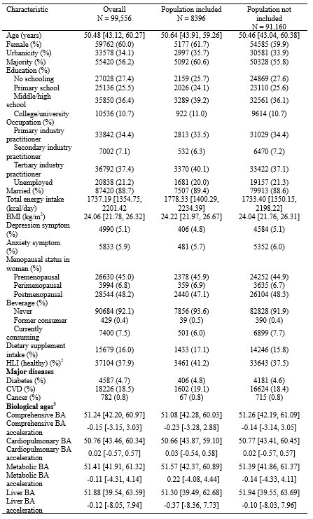
      The correlation analyses between visual acuity and MRS/EEG measures were only performed in the congenital cataract reversal group since the sighed control group comprised of individuals with vision in the normal range; thus this analyses would not make sense. Table 1 with the individual visual acuities for all participants, including the normally sighted controls, shows the low variance in the latter group.  

      For variables in which no apiori group differences in variance were predicted, we performed the correlation analyses across groups (see Supplementary Material S12, S15).

      We will highlight these motivations more clearly in the Methods of the revised manuscript.

      (9 3.4) Interpretation of Aperiodic Signal

      Relying on previous studies to interpret the aperiodic slope as a proxy for excitation/inhibition (E/I) does not make the interpretation more robust.

      How to interpret aperiodic EEG activity has been subject of extensive investigation. We cite studies which provide evidence from multiple species (monkeys, humans) and measurements (EEG, MEG, ECoG), including studies which pharmacologically manipulated E/I balance.

      Whether our findings are robust, in fact, requires a replication study. Importantly, we analyzed the intercept of the aperiodic activity fit as well, and discuss results related to the intercept.

      Quote:

      “3.4 Interpretation of aperiodic signal:

      - Several recent papers demonstrated that the aperiodic signal measured in EEG or ECoG is related to various important aspects such as age, skull thickness, electrode impedance, as well as cognition. Thus, currently, very little is known about the underlying effects which influence the aperiodic intercept and slope. The entire interpretation of the aperiodic slope as a proxy for E/I is based on a computational model and simulation (as described in the Gao et al. paper).

      Response: Apart from the modeling work from Gao et al., multiple papers which have also been cited which used ECoG, EEG and MEG and showed concomitant changes in aperiodic activity with pharmacological manipulation of the E/I ratio (Colombo et al., 2019; Molina et al., 2020; Muthukumaraswamy & Liley, 2018). Further, several prior studies have interpreted changes in the aperiodic slope as reflective of changes in the E/I ratio, including studies of developmental groups (Favaro et al., 2023; Hill et al., 2022; McSweeney et al., 2023; Schaworonkow & Voytek, 2021) as well as patient groups (Molina et al., 2020; Ostlund et al., 2021).

      - The authors further wrote: We used the slope of the aperiodic (1/f) component of the EEG spectrum as an estimate of E/I ratio (Gao et al., 2017; Medel et al., 2020; Muthukumaraswamy & Liley, 2018). This is a highly speculative interpretation with very little empirical evidence. These papers were conducted with ECoG data (mostly in animals) and mostly under anesthesia. Thus, these studies only allow an indirect interpretation by what the 1/f slope in EEG measurements is actually influenced.

      Response: Note that Muthukumaraswamy et al. (2018) used different types of pharmacological manipulations and analyzed periodic and aperiodic MEG activity in humans, in addition to monkey ECoG (Muthukumaraswamy & Liley, 2018). Further, Medel et al. (now published as Medel et al., 2023) compared EEG activity in addition to ECoG data after propofol administration. The interpretation of our results are in line with a number of recent studies in developing (Hill et al., 2022; Schaworonkow & Voytek, 2021) and special populations using EEG. As mentioned above, several prior studies have used the slope of the 1/f component/aperiodic activity as an indirect measure of the E/I ratio (Favaro et al., 2023; Hill et al., 2022; McSweeney et al., 2023; Molina et al., 2020; Ostlund et al., 2021; Schaworonkow & Voytek, 2021), including studies using scalp-recorded EEG from humans.

      In the introduction of the revised manuscript, we have made more explicit that this metric is indirect (Page 3, Line 91), (additionally see Discussion, Page 24, Lines 644-645, Page 25, Lines 650-657).

      While a full understanding of aperiodic activity needs to be provided, some convergent ideas have emerged. We think that our results contribute to this enterprise, since our study is, to the best of our knowledge, the first which assessed MRS measured neurotransmitter levels and EEG aperiodic activity.“

      (10) Additionally, the authors state:

      "We cannot think of how any of the exploratory correlations between neurophysiological measures and MRS measures could be accounted for by a difference e.g. in skull thickness."

      (11) This could be addressed directly by including skull thickness as a covariate or visualizing it in scatterplots, for instance, by representing skull thickness as the size of the dots.

      We are not aware of any study that would justify such an analysis.

      Our analyses were based on previous findings in the literature.

      Since to the best of our knowledge, no evidence exists that congenital cataracts go together with changes in skull thickness, and that skull thickness might selectively modulate visual cortex Glx/GABA+ but not NAA measures, we decided against following this suggestion.

      Notably, the neurotransmitter concentration reported here is after tissue segmentation of the voxel region. The tissue fraction was shown to not differ between groups in the MRS voxels (Supplementary Material S4). The EEG electrode impedance was lowered to <10 kOhm in every participant (Methods, Page 13, Line 344), and preparation was identical across groups.

      (12 3.5) Problems with EEG Preprocessing and Analysis

      Downsampling: The decision to downsample the data to 60 Hz "to match the stimulation rate" is problematic. This choice conflates subsequent spectral analyses due to aliasing issues, as explained by the Nyquist theorem. While the authors cite prior studies (Schwenk et al., 2020; VanRullen & MacDonald, 2012) to justify this decision, these studies focused on alpha (8-12 Hz), where aliasing is less of a concern compared of analyzing aperiodic signal. Furthermore, in contrast, the current study analyzes the frequency range from 1-20 Hz, which is too narrow for interpreting the aperiodic signal as E/I. Typically, this analysis should include higher frequencies, spanning at least 1-30 Hz or even 1-45 Hz (not 20-40 Hz).

      As mentioned in the Methods (Page 15 Line 376) and the previous response, the pop_resample function used by EEGLAB applies an anti-aliasing filter, at half the resampling frequency (as per the Nyquist theorem https://eeglab.org/tutorials/05_Preprocess/resampling.html). The upper cut off of the low pass filter set by EEGlab prior to down sampling (30 Hz) is still far above the frequency of interest in the current study  (1-20 Hz), thus allowing us to derive valid results.

      Quote:

      “- The authors downsampled the data to 60Hz to "to match the stimulation rate". What is the intention of this? Because the subsequent spectral analyses are conflated by this choice (see Nyquist theorem).

      Response: This data were collected as part of a study designed to evoke alpha activity with visual white-noise, which ranged in luminance with equal power at all frequencies from 1-60 Hz, restricted by the refresh rate of the monitor on which stimuli were presented (Pant et al., 2023). This paradigm and method was developed by VanRullen and colleagues (Schwenk et al., 2020; Vanrullen & MacDonald, 2012), wherein the analysis requires the same sampling rate between the presented frequencies and the EEG data. The downsampling function used here automatically applies an anti-aliasing filter (EEGLAB 2019) .”

      Moreover, the resting-state data were not resampled to 60 Hz. We will make this clearer in the Methods of the revised manuscript.

      Our consistent results of group differences across all three  EEG conditions, thus, exclude any possibility that they were driven by aliasing artifacts.

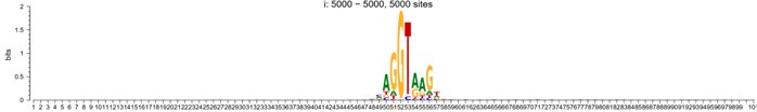
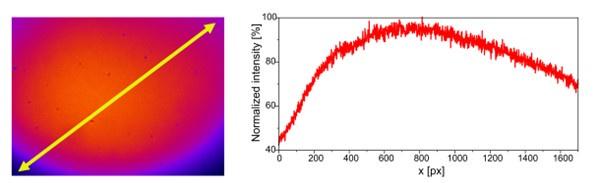
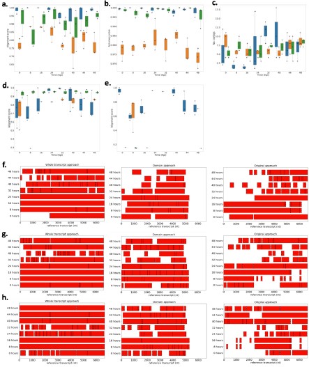
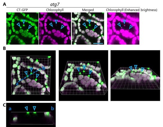
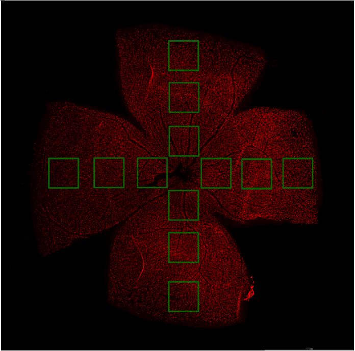
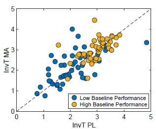
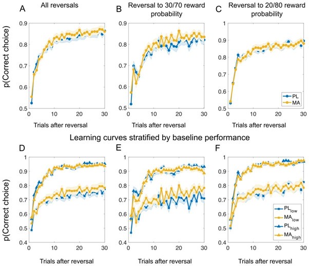
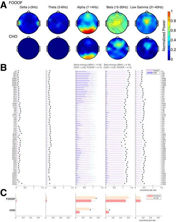
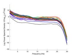
      The expected effects of this anti-aliasing filter can be seen in the attached Figure R1, showing an example participant’s spectrum in the 1-30 Hz range (as opposed to the 1-20 Hz plotted in the manuscript), clearly showing a 30-40 dB drop at 30 Hz. Any aliasing due to, for example, remaining line noise, would additionally be visible in this figure (as well as Figure 3) as a peak.

      Author response image 1.

      Power spectral density of one congenital cataract-reversal (CC) participant in the visual stimulation condition across all channels. The reduced power at 30 Hz shows the effects of the anti-aliasing filter applied by EEGLAB’s pop_resample function.

      As we stated in the manuscript, and in previous reviews, so far there has been no consensus on the exact range of measuring aperiodic activity. We made a principled decision based on the literature (showing a knee in aperiodic fits of this dataset at 20 Hz) (Medel et al., 2023; Ossandón et al., 2023), data quality (possible contamination by line noise at higher frequencies) and the purpose of the visual stimulation experiment (to look at the lower frequency range by stimulating up to 60 Hz, thereby limiting us to quantifying below 30 Hz), that 1-20 Hz would be the fit range in this dataset.

      Quote:

      “(3) What's the underlying idea of analyzing two separate aperiodic slopes (20-40Hz and 1-19Hz). This is very unusual to compute the slope between 20-40 Hz, where the SNR is rather low.

      "Ossandón et al. (2023), however, observed that in addition to the flatter slope of the aperiodic power spectrum in the high frequency range (20-40 Hz), the slope of the low frequency range (1-19 Hz) was steeper in both, congenital cataract-reversal individuals, as well as in permanently congenitally blind humans."

      Response: The present manuscript computed the slope between 1-20 Hz. Ossandón et al. as well as Medel et al. (2023) found a “knee” of the 1/f distribution at 20 Hz and describe further the motivations for computing both slope ranges. For example, Ossandón et al. used a data driven approach and compared single vs. dual fits and found that the latter fitted the data better. Additionally, they found the best fit if a knee at 20 Hz was used. We would like to point out that no standard range exists for the fitting of the 1/f component across the literature and, in fact, very different ranges have been used (Gao et al., 2017; Medel et al., 2023; Muthukumaraswamy & Liley, 2018).“

      (13) Baseline Removal: Subtracting the mean activity across an epoch as a baseline removal step is inappropriate for resting-state EEG data. This preprocessing step undermines the validity of the analysis. The EEG dataset has fundamental flaws, many of which were pointed out in the previous review round but remain unaddressed. In its current form, the manuscript falls short of standards for robust EEG analysis. If I were reviewing for another journal, I would recommend rejection based on these flaws.

      The baseline removal step from each epoch serves to remove the DC component of the recording and detrend the data. This is a standard preprocessing step (included as an option in preprocessing pipelines recommended by the EEGLAB toolbox, FieldTrip toolbox and MNE toolbox), additionally necessary to improve the efficacy of ICA decomposition (Groppe et al., 2009).

      In the previous review round, a clarification of the baseline timing was requested, which we added. Beyond this request, there was no mention of the appropriateness of the baseline removal and/or a request to provide reasons for why it might not undermine the validity of the analysis.

      Quote:

      “- "Subsequently, baseline removal was conducted by subtracting the mean activity across the length of an epoch from every data point." The actual baseline time segment should be specified.

      Response: The time segment was the length of the epoch, that is, 1 second for the resting state conditions and 6.25 seconds for the visual stimulation conditions. This has been explicitly stated in the revised manuscript (Page 13, Line 354).”

      Prior work in the time (not frequency) domain on event-related potential (ERP) analysis has suggested that the baselining step might cause spurious effects (Delorme, 2023) (although see (Tanner et al., 2016)). We did not perform ERP analysis at any stage. One recent study suggests spurious group differences in the 1/f signal might be driven by an inappropriate dB division baselining method (Gyurkovics et al., 2021), which we did not perform.

      Any effect of our baselining procedure on the FFT spectrum would be below the 1 Hz range, which we did not analyze.  

      Each of the preprocessing steps in the manuscript match pipelines described and published in extensive prior work. We document how multiple aspects of our EEG results replicate prior findings (Supplementary Material S15, S18, S19), reports of other experimenters, groups and locations, validating that our results are robust.

      We therefore reject the claim of methodological flaws in our EEG analyses in the strongest possible terms.

      Quote:

      “3.5 Problems with EEG preprocessing and analysis:

      - It seems that the authors did not identify bad channels nor address the line noise issue (even a problem if a low pass filter of below-the-line noise was applied).

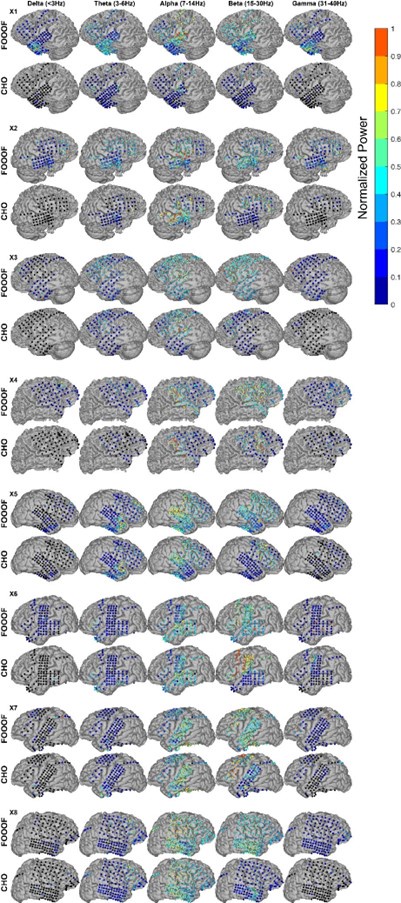
      Response: As pointed out in the methods and Figure 1, we only analyzed data from two occipital channels, O1 and O2 neither of which were rejected for any participant. Channel rejection was performed for the larger dataset, published elsewhere (Ossandón et al., 2023; Pant et al., 2023). As control sites we added the frontal channels FP1 and Fp2 (see Supplementary Material S14)

      Neither Ossandón et al. (2023) nor Pant et al. (2023) considered frequency ranges above 40 Hz to avoid any possible contamination with line noise. Here, we focused on activity between 0 and 20 Hz, definitely excluding line noise contaminations (Methods, Page 14, Lines 365-367). The low pass filter (FIR, 1-45 Hz) guaranteed that any spill-over effects of line noise would be restricted to frequencies just below the upper cutoff frequency.

      Additionally, a prior version of the analysis used spectrum interpolation to remove line noise; the group differences remained stable (Ossandón et al., 2023). We have reported this analysis in the revised manuscript (Page 14, Lines 364-357).

      Further, both groups were measured in the same lab, making line noise (~ 50 Hz) as an account for the observed group effects in the 1-20 Hz frequency range highly unlikely. Finally, any of the exploratory MRS-EEG correlations would be hard to explain if the EEG parameters would be contaminated with line noise.

      - What was the percentage of segments that needed to be rejected due to the 120μV criteria? This should be reported specifically for EO & EC and controls and patients.

      Response: The mean percentage of 1 second segments rejected for each resting state condition and the percentage of 6.25 long segments rejected in each group for the visual stimulation condition have been added to the revised manuscript (Supplementary Material S10), and referred to in the Methods on Page 14, Lines 372-373).

      - The authors downsampled the data to 60Hz to "to match the stimulation rate". What is the intention of this? Because the subsequent spectral analyses are conflated by this choice (see Nyquist theorem).

      Response: This data were collected as part of a study designed to evoke alpha activity with visual white-noise, which changed in luminance with equal power at all frequencies from 1-60 Hz, restricted by the refresh rate of the monitor on which stimuli were presented (Pant et al., 2023). This paradigm and method was developed by VanRullen and colleagues (Schwenk et al., 2020; VanRullen & MacDonald, 2012), wherein the analysis requires the same sampling rate between the presented frequencies and the EEG data. The downsampling function used here automatically applies an anti-aliasing filter (EEGLAB 2019) .

      - "Subsequently, baseline removal was conducted by subtracting the mean activity across the length of an epoch from every data point." The actual baseline time segment should be specified.

      The time segment was the length of the epoch, that is, 1 second for the resting state conditions and 6.25 seconds for the visual stimulation conditions. This has now been explicitly stated in the revised manuscript (Page 14, Lines 379-380).<br /> - "We excluded the alpha range (8-14 Hz) for this fit to avoid biasing the results due to documented differences in alpha activity between CC and SC individuals (Bottari et al., 2016; Ossandón et al., 2023; Pant et al., 2023)." This does not really make sense, as the FOOOF algorithm first fits the 1/f slope, for which the alpha activity is not relevant.

      Response: We did not use the FOOOF algorithm/toolbox in this manuscript. As stated in the Methods, we used a 1/f fit to the 1-20 Hz spectrum in the log-log space, and subtracted this fit from the original spectrum to obtain the corrected spectrum. Given the pronounced difference in alpha power between groups (Bottari et al., 2016; Ossandón et al., 2023; Pant et al., 2023), we were concerned it might drive differences in the exponent values. Our analysis pipeline had been adapted from previous publications of our group and other labs (Ossandón et al., 2023; Voytek et al., 2015; Waschke et al., 2017).

      We have conducted the analysis with and without the exclusion of the alpha range, as well as using the FOOOF toolbox both in the 1-20 Hz and 20-40 Hz ranges (Ossandón et al., 2023). The findings of a steeper slope in the 1-20 Hz range as well as lower alpha power in CC vs SC individuals remained stable. In Ossandón et al., the comparison between the piecewise fits and FOOOF fits led the authors to use the former, as it outperformed the FOOOF algorithm for their data.

      - The model fits of the 1/f fitting for EO, EC, and both participant groups should be reported.

      Response: In Figure 3 of the manuscript, we depicted the mean spectra and 1/f fits for each group.

      In the revised manuscript, we added the fit quality metrics (average R<sup>2</sup> values > 0.91 for each group and condition) (Methods Page 15, Lines 395-396; Supplementary Material S11) and additionally show individual subjects’ fits (Supplementary Material S11).“

      (14) The authors mention:

      "The EEG data sets reported here were part of data published earlier (Ossandón et al., 2023; Pant et al., 2023)." Thus, the statement "The group differences for the EEG assessments corresponded to those of a larger sample of CC individuals (n=38) " is a circular argument and should be avoided."

      The authors addressed this comment and adjusted the statement. However, I do not understand, why not the full sample published earlier (Ossandón et al., 2023) was used in the current study?

      The recording of EEG resting state data stated in 2013, while MRS testing could only be set up by the end of 2019. Moreover, not all subjects who qualify for EEG recording qualify for being scanned (e.g. due to MRI safety, claustrophobia)

      References

      Bottari, D., Troje, N. F., Ley, P., Hense, M., Kekunnaya, R., & Röder, B. (2016). Sight restoration after congenital blindness does not reinstate alpha oscillatory activity in humans. Scientific Reports. https://doi.org/10.1038/srep24683

      Colombo, M. A., Napolitani, M., Boly, M., Gosseries, O., Casarotto, S., Rosanova, M., Brichant, J. F., Boveroux, P., Rex, S., Laureys, S., Massimini, M., Chieregato, A., & Sarasso, S. (2019). The spectral exponent of the resting EEG indexes the presence of consciousness during unresponsiveness induced by propofol, xenon, and ketamine. NeuroImage, 189(September 2018), 631–644. https://doi.org/10.1016/j.neuroimage.2019.01.024

      Delorme, A. (2023). EEG is better left alone. Scientific Reports, 13(1), 2372. https://doi.org/10.1038/s41598-023-27528-0

      Favaro, J., Colombo, M. A., Mikulan, E., Sartori, S., Nosadini, M., Pelizza, M. F., Rosanova, M., Sarasso, S., Massimini, M., & Toldo, I. (2023). The maturation of aperiodic EEG activity across development reveals a progressive differentiation of wakefulness from sleep. NeuroImage, 277. https://doi.org/10.1016/J.NEUROIMAGE.2023.120264

      Gao, R., Peterson, E. J., & Voytek, B. (2017). Inferring synaptic excitation/inhibition balance from field potentials. NeuroImage, 158(March), 70–78. https://doi.org/10.1016/j.neuroimage.2017.06.078

      Groppe, D. M., Makeig, S., & Kutas, M. (2009). Identifying reliable independent components via split-half comparisons. NeuroImage, 45(4), 1199–1211. https://doi.org/10.1016/j.neuroimage.2008.12.038

      Gyurkovics, M., Clements, G. M., Low, K. A., Fabiani, M., & Gratton, G. (2021). The impact of 1/f activity and baseline correction on the results and interpretation of time-frequency analyses of EEG/MEG data: A cautionary tale. NeuroImage, 237. https://doi.org/10.1016/j.neuroimage.2021.118192

      Hill, A. T., Clark, G. M., Bigelow, F. J., Lum, J. A. G., & Enticott, P. G. (2022). Periodic and aperiodic neural activity displays age-dependent changes across early-to-middle childhood. Developmental Cognitive Neuroscience, 54, 101076. https://doi.org/10.1016/J.DCN.2022.101076

      Maurer, D., Mondloch, C. J., & Lewis, T. L. (2007). Sleeper effects. In Developmental Science. https://doi.org/10.1111/j.1467-7687.2007.00562.x

      McSweeney, M., Morales, S., Valadez, E. A., Buzzell, G. A., Yoder, L., Fifer, W. P., Pini, N., Shuffrey, L. C., Elliott, A. J., Isler, J. R., & Fox, N. A. (2023). Age-related trends in aperiodic EEG activity and alpha oscillations during early- to middle-childhood. NeuroImage, 269, 119925. https://doi.org/10.1016/j.neuroimage.2023.119925

      Medel, V., Irani, M., Crossley, N., Ossandón, T., & Boncompte, G. (2023). Complexity and 1/f slope jointly reflect brain states. Scientific Reports, 13(1), 21700. https://doi.org/10.1038/s41598-023-47316-0

      Molina, J. L., Voytek, B., Thomas, M. L., Joshi, Y. B., Bhakta, S. G., Talledo, J. A., Swerdlow, N. R., & Light, G. A. (2020). Memantine Effects on Electroencephalographic Measures of Putative Excitatory/Inhibitory Balance in Schizophrenia. Biological Psychiatry: Cognitive Neuroscience and Neuroimaging, 5(6), 562–568. https://doi.org/10.1016/j.bpsc.2020.02.004

      Muthukumaraswamy, S. D., & Liley, D. T. (2018). 1/F electrophysiological spectra in resting and drug-induced states can be explained by the dynamics of multiple oscillatory relaxation processes. NeuroImage, 179(November 2017), 582–595. https://doi.org/10.1016/j.neuroimage.2018.06.068

      Ossandón, J. P., Stange, L., Gudi-Mindermann, H., Rimmele, J. M., Sourav, S., Bottari, D., Kekunnaya, R., & Röder, B. (2023). The development of oscillatory and aperiodic resting state activity is linked to a sensitive period in humans. NeuroImage, 275, 120171. https://doi.org/10.1016/J.NEUROIMAGE.2023.120171

      Ostlund, B. D., Alperin, B. R., Drew, T., & Karalunas, S. L. (2021). Behavioral and cognitive correlates of the aperiodic (1/f-like) exponent of the EEG power spectrum in adolescents with and without ADHD. Developmental Cognitive Neuroscience, 48, 100931. https://doi.org/10.1016/j.dcn.2021.100931

      Pant, R., Ossandón, J., Stange, L., Shareef, I., Kekunnaya, R., & Röder, B. (2023). Stimulus-evoked and resting-state alpha oscillations show a linked dependence on patterned visual experience for development. NeuroImage: Clinical, 103375. https://doi.org/10.1016/J.NICL.2023.103375

      Schaworonkow, N., & Voytek, B. (2021). Longitudinal changes in aperiodic and periodic activity in electrophysiological recordings in the first seven months of life. Developmental Cognitive Neuroscience, 47. https://doi.org/10.1016/j.dcn.2020.100895

      Schwenk, J. C. B., VanRullen, R., & Bremmer, F. (2020). Dynamics of Visual Perceptual Echoes Following Short-Term Visual Deprivation. Cerebral Cortex Communications, 1(1). https://doi.org/10.1093/TEXCOM/TGAA012

      Tanner, D., Norton, J. J. S., Morgan-Short, K., & Luck, S. J. (2016). On high-pass filter artifacts (they’re real) and baseline correction (it’s a good idea) in ERP/ERMF analysis. Journal of Neuroscience Methods, 266, 166–170. https://doi.org/10.1016/j.jneumeth.2016.01.002

      Vanrullen, R., & MacDonald, J. S. P. (2012). Perceptual echoes at 10 Hz in the human brain. Current Biology. https://doi.org/10.1016/j.cub.2012.03.050

      Voytek, B., Kramer, M. A., Case, J., Lepage, K. Q., Tempesta, Z. R., Knight, R. T., & Gazzaley, A. (2015). Age-related changes in 1/f neural electrophysiological noise. Journal of Neuroscience, 35(38). https://doi.org/10.1523/JNEUROSCI.2332-14.2015

      Waschke, L., Wöstmann, M., & Obleser, J. (2017). States and traits of neural irregularity in the age-varying human brain. Scientific Reports 2017 7:1, 7(1), 1–12. https://doi.org/10.1038/s41598-017-17766-4


      The following is the authors’ response to the original reviews.

      eLife Assessment

      This potentially useful study involves neuro-imaging and electrophysiology in a small cohort of congenital cataract patients after sight recovery and age-matched control participants with normal sight. It aims to characterize the effects of early visual deprivation on excitatory and inhibitory balance in the visual cortex. While the findings are taken to suggest the existence of persistent alterations in Glx/GABA ratio and aperiodic EEG signals, the evidence supporting these claims is incomplete. Specifically, small sample sizes, lack of a specific control cohort, and other methodological limitations will likely restrict the usefulness of the work, with relevance limited to scientists working in this particular subfield.

      As pointed out in the public reviews, there are very few human models which allow for assessing the role of early experience on neural circuit development. While the prevalent research in permanent congenital blindness reveals the response and adaptation of the developing brain to an atypical situation (blindness), research in sight restoration addresses the question of whether and how atypical development can be remediated if typical experience (vision) is restored. The literature on the role of visual experience in the development of E/I balance in humans, assessed via Magnetic Resonance Spectroscopy (MRS), has been limited to a few studies on congenital permanent blindness. Thus, we assessed sight recovery individuals with a history of congenital blindness, as limited evidence from other researchers indicated that the visual cortex E/I ratio might differ compared to normally sighted controls.

      Individuals with total bilateral congenital cataracts who remained untreated until later in life are extremely rare, particularly if only carefully diagnosed patients are included in a study sample. A sample size of 10 patients is, at the very least, typical of past studies in this population, even for exclusively behavioral assessments. In the present study, in addition to behavioral assessment as an indirect measure of sensitive periods, we investigated participants with two neuroimaging methods (Magnetic Resonance Spectroscopy and electroencephalography) to directly assess the neural correlates of sensitive periods in humans. The electroencephalography data allowed us to link the results of our small sample to findings documented in large cohorts of both, sight recovery individuals and permanently congenitally blind individuals. As pointed out in a recent editorial recommending an “exploration-then-estimation procedure,” (“Consideration of Sample Size in Neuroscience Studies,” 2020), exploratory studies like ours provide crucial direction and specific hypotheses for future work.

      We included an age-matched sighted control group recruited from the same community, measured in the same scanner and laboratory, to assess whether early experience is necessary for a typical excitatory/inhibitory (E/I) ratio to emerge in adulthood. The present findings indicate that this is indeed the case. Based on these results, a possible question to answer in future work, with individuals who had developmental cataracts, is whether later visual deprivation causes similar effects. Note that even if visual deprivation at a later stage in life caused similar effects, the current results would not be invalidated; by contrast, they are essential to understand future work on late (permanent or transient) blindness.

      Thus, we think that the present manuscript has far reaching implications for our understanding of the conditions under which E/I balance, a crucial characteristic of brain functioning, emerges in humans.

      Finally, our manuscript is one of the first few studies that relate MRS neurotransmitter concentrations to parameters of EEG aperiodic activity. Since present research has been using aperiodic activity as a correlate of the E/I ratio, and partially of higher cognitive functions, we think that our manuscript additionally contributes to a better understanding of what might be measured with aperiodic neurophysiological activity.

      Public Reviews:<br /> Reviewer #1 (Public Review):

      Summary:

      In this human neuroimaging and electrophysiology study, the authors aimed to characterize the effects of a period of visual deprivation in the sensitive period on excitatory and inhibitory balance in the visual cortex. They attempted to do so by comparing neurochemistry conditions ('eyes open', 'eyes closed') and resting state, and visually evoked EEG activity between ten congenital cataract patients with recovered sight (CC), and ten age-matched control participants (SC) with normal sight.

      First, they used magnetic resonance spectroscopy to measure in vivo neurochemistry from two locations, the primary location of interest in the visual cortex, and a control location in the frontal cortex. Such voxels are used to provide a control for the spatial specificity of any effects because the single-voxel MRS method provides a single sampling location. Using MR-visible proxies of excitatory and inhibitory neurotransmission, Glx and GABA+ respectively, the authors report no group effects in GABA+ or Glx, no difference in the functional conditions 'eyes closed' and 'eyes open'. They found an effect of the group in the ratio of Glx/GABA+ and no similar effect in the control voxel location. They then performed multiple exploratory correlations between MRS measures and visual acuity, and reported a weak positive correlation between the 'eyes open' condition and visual acuity in CC participants.

      The same participants then took part in an EEG experiment. The authors selected only two electrodes placed in the visual cortex for analysis and reported a group difference in an EEG index of neural activity, the aperiodic intercept, as well as the aperiodic slope, considered a proxy for cortical inhibition. They report an exploratory correlation between the aperiodic intercept and Glx in one out of three EEG conditions.

      The authors report the difference in E/I ratio, and interpret the lower E/I ratio as representing an adaptation to visual deprivation, which would have initially caused a higher E/I ratio. Although intriguing, the strength of evidence in support of this view is not strong. Amongst the limitations are the low sample size, a critical control cohort that could provide evidence for a higher E/I ratio in CC patients without recovered sight for example, and lower data quality in the control voxel.

      Strengths of study:

      How sensitive period experience shapes the developing brain is an enduring and important question in neuroscience. This question has been particularly difficult to investigate in humans. The authors recruited a small number of sight-recovered participants with bilateral congenital cataracts to investigate the effect of sensitive period deprivation on the balance of excitation and inhibition in the visual brain using measures of brain chemistry and brain electrophysiology. The research is novel, and the paper was interesting and well-written.

      Limitations:

      (1.1) Low sample size. Ten for CC and ten for SC, and a further two SC participants were rejected due to a lack of frontal control voxel data. The sample size limits the statistical power of the dataset and increases the likelihood of effect inflation.

      Applying strict criteria, we only included individuals who were born with no patterned vision in the CC group. The population of individuals who have remained untreated past infancy is small in India, despite a higher prevalence of childhood cataract than Germany. Indeed, from the original 11 CC and 11 SC participants tested, one participant each from the CC and SC group had to be rejected, as their data had been corrupted, resulting in 10 participants in each group.

      It was a challenge to recruit participants from this rare group with no history of neurological diagnosis/intake of neuromodulatory medications, who were able and willing to undergo both MRS and EEG. For this study, data collection took more than 2.5 years.

      We took care of the validity of our results with two measures; first, we assessed not just MRS, but additionally, EEG measures of E/I ratio. The latter allowed us to link results to a larger population of CC individuals, that is, we replicated the results of a larger group of 28 additional individuals (Ossandón et al., 2023) in our sub-group.

      Second, we included a control voxel. As predicted, all group effects were restricted to the occipital voxel.

      (1.2) Lack of specific control cohort. The control cohort has normal vision. The control cohort is not specific enough to distinguish between people with sight loss due to different causes and patients with congenital cataracts with co-morbidities. Further data from more specific populations, such as patients whose cataracts have not been removed, with developmental cataracts, or congenitally blind participants, would greatly improve the interpretability of the main finding. The lack of a more specific control cohort is a major caveat that limits a conclusive interpretation of the results.

      The existing work on visual deprivation and neurochemical changes, as assessed with MRS, has been limited to permanent congenital blindness. In fact, most of the studies on permanent blindness included only congenitally blind or early blind humans (Coullon et al., 2015; Weaver et al., 2013), or, in separate studies, only late-blind individuals (Bernabeu et al., 2009). Thus, accordingly, we started with the most “extreme” visual deprivation model, sight recovery after congenital blindness. If we had not observed any group difference compared to normally sighted controls, investigating other groups might have been trivial. Based on our results, subsequent studies in late blind individuals, and then individuals with developmental cataracts, can be planned with clear hypotheses.

      (1.3) MRS data quality differences. Data quality in the control voxel appears worse than in the visual cortex voxel. The frontal cortex MRS spectrum shows far broader linewidth than the visual cortex (Supplementary Figures). Compared to the visual voxel, the frontal cortex voxel has less defined Glx and GABA+ peaks; lower GABA+ and Glx concentrations, lower NAA SNR values; lower NAA concentrations. If the data quality is a lot worse in the FC, then small effects may not be detectable.

      Worse data quality in the frontal than the visual cortex has been repeatedly observed in the MRS literature, attributable to magnetic field distortions (Juchem & Graaf, 2017) resulting from the proximity of the region to the sinuses (recent example: (Rideaux et al., 2022)). Nevertheless, we chose the frontal control region rather than a parietal voxel, given the potential neurochemical changes in multisensory regions of the parietal cortex due to blindness. Such reorganization would be less likely in frontal areas associated with higher cognitive functions. Further, prior MRS studies of the visual cortex have used the frontal cortex as a control region as well (Pitchaimuthu et al., 2017; Rideaux et al., 2022). In the revised manuscript, we more explicitly inform the reader about this data quality difference between regions in the Methods (Pages 11-12, MRS Data Quality/Table 2) and Discussion (Page 25, Lines 644- 647).

      Importantly, while in the present study data quality differed between the frontal and visual cortex voxel, it did not differ between groups (Supplementary Material S6).  

      Further, we checked that the frontal cortex datasets for Glx and GABA+ concentrations were of sufficient quality: the fit error was below 8.31% in both groups (Supplementary Material S3). For reference, Mikkelsen et al. reported a mean GABA+ fit error of 6.24 +/- 1.95% from a posterior cingulate cortex voxel across 8 GE scanners, using the Gannet pipeline. No absolute cutoffs have been proposed for fit errors. However, MRS studies in special populations (I/E ratio assessed in narcolepsy (Gao et al., 2024), GABA concentration assessed in Autism Spectrum Disorder (Maier et al., 2022) have used frontal cortex data with a fit error of <10% to identify differences between cohorts (Gao et al., 2024; Pitchaimuthu et al., 2017). Based on the literature, MRS data from the frontal voxel of the present study would have been of sufficient quality to uncover group differences.

      In the revised manuscript, we added the recently published MRS quality assessment form to the supplementary materials (Supplementary Excel File S1). Additionally, we would like to allude to our apriori prediction of group differences for the visual cortex, but not for the frontal cortex voxel. Finally, EEG data quality did not differ between frontal and occipital electrodes; therefore, lower sensitivity of frontal measures cannot easily explain the lack of group differences for frontal measures.

      (1.4) Because of the direction of the difference in E/I, the authors interpret their findings as representing signatures of sight improvement after surgery without further evidence, either within the study or from the literature. However, the literature suggests that plasticity and visual deprivation drive the E/I index up rather than down. Decreasing GABA+ is thought to facilitate experience-dependent remodelling. What evidence is there that cortical inhibition increases in response to a visual cortex that is over-sensitised due to congenital cataracts? Without further experimental or literature support this interpretation remains very speculative.

      Indeed, higher inhibition was not predicted, which we attempt to reconcile in our discussion section. We base our discussion mainly on the non-human animal literature, which has shown evidence of homeostatic changes after prolonged visual deprivation in the adult brain (Barnes et al., 2015). It is also interesting to note that after monocular deprivation in adult humans, resting GABA+ levels decreased in the visual cortex (Lunghi et al., 2015). Assuming that after delayed sight restoration, adult neuroplasticity mechanisms must be employed, these studies would predict a “balancing” of the increased excitatory drive following sight restoration by a commensurate increase in inhibition (Keck et al., 2017). Additionally, the EEG results of the present study allowed for speculation regarding the underlying neural mechanisms of an altered E/I ratio. The aperiodic EEG activity suggested higher spontaneous spiking (increased intercept) and increased inhibition (steeper aperiodic slope between 1-20 Hz) in CC vs SC individuals (Ossandón et al., 2023).

      In the revised manuscript, we have more clearly indicated that these speculations are based primarily on non-human animal work, due to the lack of human studies on the subject (Page 23, Lines 609-613).

      (1.5) Heterogeneity in the patient group. Congenital cataract (CC) patients experienced a variety of duration of visual impairment and were of different ages. They presented with co-morbidities (absorbed lens, strabismus, nystagmus). Strabismus has been associated with abnormalities in GABAergic inhibition in the visual cortex. The possible interactions with residual vision and confounds of co-morbidities are not experimentally controlled for in the correlations, and not discussed.

      The goal of the present study was to assess whether we would observe changes in E/I ratio after restoring vision at all. We would not have included patients without nystagmus in the CC group of the present study, since it would have been unlikely that they experienced congenital patterned visual deprivation. Amongst diagnosticians, nystagmus or strabismus might not be considered genuine “comorbidities” that emerge in people with congenital cataracts. Rather, these are consequences of congenital visual deprivation, which we employed as diagnostic criteria. Similarly, absorbed lenses are clear signs that cataracts were congenital. As in other models of experience dependent brain development (e.g. the extant literature on congenital permanent blindness, including anophthalmic individuals (Coullon et al., 2015; Weaver et al., 2013), some uncertainty remains regarding whether the (remaining, in our case) abnormalities of the eye, or the blindness they caused, are the factors driving neural changes. In case of people with reversed congenital cataracts, at least the retina is considered to be intact, as they would otherwise not receive cataract removal surgery.

      However, we consider it unlikely that strabismus caused the group differences, because the present study shows group differences in the Glx/GABA+ ratio at rest, regardless of eye opening or eye closure, for which strabismus would have caused distinct effects. By contrast, the link between GABA concentration and, for example, interocular suppression in strabismus, have so far been documented during visual stimulation (Mukerji et al., 2022; Sengpiel et al., 2006), and differed in direction depending on the amblyopic vs. non-amblyopic eye. Further, one MRS study did not find group differences in GABA concentration between the visual cortices of 16 amblyopic individuals and sighted controls (Mukerji et al., 2022), supporting that the differences in Glx/GABA+ concentration which we observed were driven by congenital deprivation, and not amblyopia-associated visual acuity or eye movement differences. 

      In the revised manuscript, we discussed the inclusion criteria in more detail, and the aforementioned reasons why our data remains interpretable (Page 5, Lines 143 – 145, Lines 147-149). 

      (1.6) Multiple exploratory correlations were performed to relate MRS measures to visual acuity (shown in Supplementary Materials), and only specific ones were shown in the main document. The authors describe the analysis as exploratory in the 'Methods' section. Furthermore, the correlation between visual acuity and E/I metric is weak, and not corrected for multiple comparisons. The results should be presented as preliminary, as no strong conclusions can be made from them. They can provide a hypothesis to test in a future study.

      In the revised manuscript, we have clearly indicated that the exploratory correlation analyses are reported to put forth hypotheses for future studies (Page 4, Lines 118-128; Page 5, Lines 132-134; Page 25, Lines 644- 647).

      (1.7) P.16 Given the correlation of the aperiodic intercept with age ("Age negatively correlated with the aperiodic intercept across CC and SC individuals, that is, a flattening of the intercept was observed with age"), age needs to be controlled for in the correlation between neurochemistry and the aperiodic intercept. Glx has also been shown to negatively correlate with age.

      The correlation between chronological age and aperiodic intercept was observed across groups, but the correlation between Glx and the intercept of the aperiodic EEG activity was seen only in the CC group, even though the SC group was matched for age. Thus, such a correlation was very unlikely to be predominantly driven by an effect of chronological age.

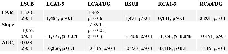
      In the revised manuscript, we added the linear regressions with age as a covariate (Supplementary Material S16, referred to in the main Results, Page 21, Lines 534-537), demonstrating the significant relationship between aperiodic intercept and Glx concentration in the CC group. 

      (1.8) Multiple exploratory correlations were performed to relate MRS to EEG measures (shown in Supplementary Materials), and only specific ones were shown in the main document. Given the multiple measures from the MRS, the correlations with the EEG measures were exploratory, as stated in the text, p.16, and in Figure 4. Yet the introduction said that there was a prior hypothesis "We further hypothesized that neurotransmitter changes would relate to changes in the slope and intercept of the EEG aperiodic activity in the same subjects." It would be great if the text could be revised for consistency and the analysis described as exploratory.

      In the revised manuscript, we improved the phrasing (Page 5, Lines 130-132) and consistently reported the correlations as exploratory in the Methods and Discussion. We consider the correlation analyses as exploratory due to our sample size and the absence of prior work. However, we did hypothesize that both MRS and EEG markers would concurrently be altered in CC vs SC individuals.

      (1.9) The analysis for the EEG needs to take more advantage of the available data. As far as I understand, only two electrodes were used, yet far more were available as seen in their previous study (Ossandon et al., 2023). The spatial specificity is not established. The authors could use the frontal cortex electrode (FP1, FP2) signals as a control for spatial specificity in the group effects, or even better, all available electrodes and correct for multiple comparisons. Furthermore, they could use the aperiodic intercept vs Glx in SC to evaluate the specificity of the correlation to CC.

      The aperiodic intercept and slope did not differ between CC and SC individuals for Fp1 and Fp2, suggesting the spatial specificity of the results. In the revised manuscript, we added this analysis to the Supplementary Material (Supplementary Material S14) and referred to it in our Results (Page 20, Lines 513-514).

      Further, Glx concentration in the visual cortex did not correlate with the aperiodic intercept in the SC group (Figure 4), suggesting that this relationship was indeed specific to the CC group.

      The data from all electrodes has been analyzed and published in other studies as well (Pant et al., 2023; Ossandón et al., 2023). 

      Reviewer #2 (Public Review):

      Summary:

      The manuscript reports non-invasive measures of activity and neurochemical profiles of the visual cortex in congenitally blind patients who recovered vision through the surgical removal of bilateral dense cataracts. The declared aim of the study is to find out how restoring visual function after several months or years of complete blindness impacts the balance between excitation and inhibition in the visual cortex.

      Strengths:

      The findings are undoubtedly useful for the community, as they contribute towards characterising the many ways this special population differs from normally sighted individuals. The combination of MRS and EEG measures is a promising strategy to estimate a fundamental physiological parameter - the balance between excitation and inhibition in the visual cortex, which animal studies show to be heavily dependent upon early visual experience. Thus, the reported results pave the way for further studies, which may use a similar approach to evaluate more patients and control groups.

      Weaknesses:

      (2.1) The main issue is the lack of an appropriate comparison group or condition to delineate the effect of sight recovery (as opposed to the effect of congenital blindness). Few previous studies suggested an increased excitation/Inhibition ratio in the visual cortex of congenitally blind patients; the present study reports a decreased E/I ratio instead. The authors claim that this implies a change of E/I ratio following sight recovery. However, supporting this claim would require showing a shift of E/I after vs. before the sight-recovery surgery, or at least it would require comparing patients who did and did not undergo the sight-recovery surgery (as common in the field).

      Longitudinal studies would indeed be the best way to test the hypothesis that the lower E/I ratio in the CC group observed by the present study is a consequence of sight restoration.

      We have now explicitly stated this in the Limitations section (Page 25, Lines 654-655).

      However, longitudinal studies involving neuroimaging are an effortful challenge, particularly in research conducted outside of major developed countries and dedicated neuroimaging research facilities. Crucially, however, had CC and SC individuals, as well as permanently congenitally blind vs SC individuals (Coullon et al., 2015; Weaver et al., 2013), not differed on any neurochemical markers, such a longitudinal study might have been trivial. Thus, in order to justify and better tailor longitudinal studies, cross-sectional studies are an initial step.

      (2.2) MR Spectroscopy shows a reduced GLX/GABA ratio in patients vs. sighted controls; however, this finding remains rather isolated, not corroborated by other observations. The difference between patients and controls only emerges for the GLX/GABA ratio, but there is no accompanying difference in either the GLX or the GABA concentrations. There is an attempt to relate the MRS data with acuity measurements and electrophysiological indices, but the explorative correlational analyses do not help to build a coherent picture. A bland correlation between GLX/GABA and visual impairment is reported, but this is specific to the patients' group (N=10) and would not hold across groups (the correlation is positive, predicting the lowest GLX/GABA ratio values for the sighted controls - the opposite of what is found). There is also a strong correlation between GLX concentrations and the EEG power at the lowest temporal frequencies. Although this relation is intriguing, it only holds for a very specific combination of parameters (of the many tested): only with eyes open, only in the patient group.

      We interpret these findings differently, that is, in the context of experiments from non-human animals and the larger MRS literature (Page 23, Lines 609-611).

      Homeostatic control of E/I balance assumes that the ratio of excitation (reflected here by Glx) and inhibition (reflected here by GABA+) is regulated. Like prior work (Gao et al., 2024, 2024; Narayan et al., 2022; Perica et al., 2022; Steel et al., 2020; Takado et al., 2022; Takei et al., 2016), we assumed that the ratio of Glx/GABA+ is indicative of E/I balance rather than solely the individual neurotransmitter levels. One of the motivations for assessing the ratio vs the absolute concentration is that as per the underlying E/I balance hypothesis, a change in excitation would cause a concomitant change in inhibition, and vice versa, which has been shown in non-human animal work (Fang et al., 2021; Haider et al., 2006; Tao & Poo, 2005) and modeling research (Vreeswijk & Sompolinsky, 1996; Wu et al., 2022). Importantly, our interpretation of the lower E/I ratio is not just from the Glx/GABA+ ratio, but additionally, based on the steeper EEG aperiodic slope (1-20 Hz). 

      As stated in the Discussion section and Response 1.4, we did not expect to see a lower Glx/GABA+ ratio in CC individuals. We discuss the possible reasons for the direction of the correlation with visual acuity and aperiodic offset during passive visual stimulation, and offer interpretations and (testable) hypotheses.

      We interpret the direction of the Glx/GABA+ correlation with visual acuity to imply that patients with highest (compensatory) balancing of the consequences of congenital blindness (hyperexcitation), in light of visual stimulation, are those who recover best. Note, the sighted control group was selected based on their “normal” vision. Thus, clinical visual acuity measures are not expected to sufficiently vary, nor have the resolution to show strong correlations with neurophysiological measures. By contrast, the CC group comprised patients highly varying in visual outcomes, and thus were ideal to investigate such correlations.

      This holds for the correlation between Glx and the aperiodic intercept, as well. Previous work has suggested that the intercept of the aperiodic activity is associated with broadband spiking activity in neural circuits (Manning et al., 2009). Thus, an atypical increase of spiking activity during visual stimulation, as indirectly suggested by “old” non-human primate work on visual deprivation (Hyvärinen et al., 1981) might drive a correlation not observed in healthy populations.

      In the revised manuscript, we have more clearly indicated in the Discussion that these are possible post-hoc interpretations (Page 23, Lines 584-586; Page 24, Lines 609-620; Page 24, Lines 644-647; Pages 25, Lines 650 - 657). We argue that given the lack of such studies in humans, it is all the more important that extant data be presented completely, even if the direction of the effects are not as expected.

      (2.3) For these reasons, the reported findings do not allow us to draw firm conclusions on the relation between EEG parameters and E/I ratio or on the impact of early (vs. late) visual experience on the excitation/inhibition ratio of the human visual cortex.

      Indeed, the correlations we have tested between the E/I ratio and EEG parameters were exploratory, and have been reported as such.

      We have now made this clear in all the relevant parts of the manuscript (Introduction, Page 5, Lines 132-135; Methods, Page 16, Line 415; Results, Page 21, Figure 4; Discussion, Page 22, Line 568, Page 25, Lines 644-645, Page 25, Lines 650-657).

      The goal of our study was not to compare the effects of early vs. late visual experience. The goal was to study whether early visual experience is necessary for a typical E/I ratio in visual neural circuits. We provided clear evidence in favor of this hypothesis. Thus, the present results suggest the necessity of investigating the effects of late visual deprivation. In fact, such research is missing in permanent blindness as well.

      Reviewer #3 (Public Review):

      This manuscript examines the impact of congenital visual deprivation on the excitatory/inhibitory (E/I) ratio in the visual cortex using Magnetic Resonance Spectroscopy (MRS) and electroencephalography (EEG) in individuals whose sight was restored. Ten individuals with reversed congenital cataracts were compared to age-matched, normally sighted controls, assessing the cortical E/I balance and its interrelationship to visual acuity. The study reveals that the Glx/GABA ratio in the visual cortex and the intercept and aperiodic signal are significantly altered in those with a history of early visual deprivation, suggesting persistent neurophysiological changes despite visual restoration.

      My expertise is in EEG (particularly in the decomposition of periodic and aperiodic activity) and statistical methods. I have several major concerns in terms of methodological and statistical approaches along with the (over)interpretation of the results. These major concerns are detailed below.

      (3.1) Variability in visual deprivation:

      - The document states a large variability in the duration of visual deprivation (probably also the age at restoration), with significant implications for the sensitivity period's impact on visual circuit development. The variability and its potential effects on the outcomes need thorough exploration and discussion.

      We work with a rare, unique patient population, which makes it difficult to systematically assess the effects of different visual histories while maintaining stringent inclusion criteria such as complete patterned visual deprivation at birth. Regardless, we considered the large variance in age at surgery and time since surgery as supportive of our interpretation: group differences were found despite the large variance in duration of visual deprivation. Moreover, the existing variance was used to explore possible associations between behavior and neural measures, as well as neurochemical and EEG measures.

      In the revised manuscript, we have detailed the advantages (Methods, Page 5, Lines 143 – 145, Lines 147-149; Discussion, Page 26, Lines 677-678) and disadvantages (Discussion, Page 25, Lines 650-657) of our CC sample, with respect to duration of congenital visual deprivation.

      (3.2) Sample size:

      - The small sample size is a major concern as it may not provide sufficient power to detect subtle effects and/or overestimate significant effects, which then tend not to generalize to new data. One of the biggest drivers of the replication crisis in neuroscience.

      We address the small sample size in our Discussion, and make clear that small sample sizes were due to the nature of investigations in special populations. In the revised manuscript, we added the sample sizes of previous studies using MRS in permanently blind individuals (Page 4, Lines 108 - 109). It is worth noting that our EEG results fully align with those of larger samples of congenital cataract reversal individuals (Page 25, Lines 666-676, Supplementary Material S18, S19) (Ossandón et al., 2023), providing us confidence about their validity and reproducibility. Moreover, our MRS results and correlations of those with EEG parameters were spatially specific to occipital cortex measures.

      The main problem with the correlation analyses between MRS and EEG measures is that the sample size is simply too small to conduct such an analysis. Moreover, it is unclear from the methods section that this analysis was only conducted in the patient group (which the reviewer assumed from the plots), and not explained why this was done only in the patient group. I would highly recommend removing these correlation analyses.

      In the revised manuscript, we have more clearly marked the correlation analyses as exploratory (Introduction, Page 4, Lines 118-128 and Page 5, Lines 132-134; Methods Page 16, Line 415; Discussion Page 22, Line 568, Page 24, Lines 644-645, Page 25, Lines 650-657); note that we do not base most of our discussion on the results of these analyses.

      As indicated by Reviewer 1, reporting them allows for deriving more precise hypothesis for future studies. It has to be noted that we investigate an extremely rare population, tested outside of major developed economies and dedicated neuroimaging research facilities. In addition to being a rare patient group, these individuals come from poor communities. Therefore, we consider it justified to report these correlations as exploratory, providing direction for future research.

      (3.3) Statistical concerns:

      - The statistical analyses, particularly the correlations drawn from a small sample, may not provide reliable estimates (see https://www.sciencedirect.com/science/article/pii/S0092656613000858, which clearly describes this problem).

      It would undoubtedly be better to have a larger sample size. We nonetheless think it is of value to the research community to publish this dataset, since 10 multimodal data sets from a carefully diagnosed, rare population, representing a human model for the effects of early experience on brain development, are quite a lot. Sample sizes in prior neuroimaging studies in transient blindness have most often ranged from n = 1 to n = 10. They nevertheless provided valuable direction for future research, and integration of results across multiple studies provides scientific insights. 

      Identifying possible group differences was the goal of our study, with the correlations being an exploratory analysis, which we have clearly indicated in the methods, results and discussion.

      - Statistical analyses for the MRS: The authors should consider some additional permutation statistics, which are more suitable for small sample sizes. The current statistical model (2x2) design ANOVA is not ideal for such small sample sizes. Moreover, it is unclear why the condition (EO & EC) was chosen as a predictor and not the brain region (visual & frontal) or neurochemicals. Finally, the authors did not provide any information on the alpha level nor any information on correction for multiple comparisons (in the methods section). Finally, even if the groups are matched w.r.t. age, the time between surgery and measurement, the duration of visual deprivation, (and sex?), these should be included as covariates as it has been shown that these are highly related to the measurements of interest (especially for the EEG measurements) and the age range of the current study is large.

      In our ANOVA models, the neurochemicals were the outcome variables, and the conditions were chosen as predictors based on prior work suggesting that Glx/GABA+ might vary with eye closure (Kurcyus et al., 2018). The study was designed based on a hypothesis of group differences localized to the occipital cortex, due to visual deprivation. The frontal cortex voxel was chosen to indicate whether these differences were spatially specific. Therefore, we conducted separate ANOVAs based on this study design.

      We have now clarified the motivation for these conditions in the Introduction (Page 4, Lines 122-125) and the Methods (Page 9, Lines 219-224).

      In the revised manuscript, we added the rationale for parametric analyses for our outcomes (Shapiro-Wilk as well as Levene’s tests, Supplementary Material S9). Note that in the Supplementary Materials (S12, S14), we have reported the correlations between visual history metrics and MRS/EEG outcomes, thereby investigating whether the variance in visual history might have driven these results. Specifically, we found a (negative) correlation between visual cortex Glx/GABA+ concentration during eye closure and the visual acuity in the CC group (Figure 2c). None of the other exploratory correlations between MRS/EEG outcomes vs time since surgery, duration of blindness or visual acuity were significant in the CC group (Supplementary Material S12, S15).  

      The alpha level used for the ANOVA models specified in the Methods section was 0.05. The alpha level for the exploratory analyses reported in the main manuscript was 0.008, after correcting for (6) multiple comparisons using the Bonferroni correction, also specified in the Methods. Note that the p-values following correction are expressed as multiplied by 6, due to most readers assuming an alpha level of 0.05 (see response regarding large p-values).

      We used a control group matched for age, recruited and tested in the same institutes, using the same setup. We feel that we followed the gold standards for recruiting a healthy control group for a patient group.

      - EEG statistical analyses: The same critique as for the MRS statistical analyses applies to the EEG analysis. In addition: was the 2x3 ANOVA conducted for EO and EC independently? This seems to be inconsistent with the approach in the MRS analyses, in which the authors chose EO & EC as predictors in their 2x2 ANOVA.

      The 2x3 ANOVA was not conducted independently for the eyes open/eyes closed condition. The ANOVA conducted on the EEG metrics was 2x3 because it had two groups (CC, SC) and three conditions (eyes open (EO), eyes closed (EC) and visual stimulation (LU)) as predictors.

      - Figure 4: The authors report a p-value of >0.999 with a correlation coefficient of -0.42 with a sample size of 10 subjects. This can't be correct (it should be around: p = 0.22). All statistical analyses should be checked.

      As specified in the Methods and Figure legend, the reported p values in Figure 4 have been corrected using the Bonferroni correction, and therefore multiplied by the number of comparisons, leading to the seemingly large values.

      Additionally, to check all statistical analyses, we put the manuscript through an independent Statistics Check (Nuijten & Polanin, 2020) (https://michelenuijten.shinyapps.io/statcheck-web/) and have uploaded the consistency report with the revised Supplementary Material (Supplementary Report 1).

      - Figure 2c. Eyes closed condition: The highest score of the *Glx/GABA ratio seems to be ~3.6. In subplot 2a, there seem to be 3 subjects that show a Glx/GABA ratio score > 3.6. How can this be explained? There is also a discrepancy for the eyes-closed condition.

      The three subjects that show the Glx/GABA+ ratio > 3.6 in subplot 2a are in the SC group, whereas the correlations plotted in figure 2c are only for the CC group, where the highest score is indeed ~3.6.

      (3.4) Interpretation of aperiodic signal:

      - Several recent papers demonstrated that the aperiodic signal measured in EEG or ECoG is related to various important aspects such as age, skull thickness, electrode impedance, as well as cognition. Thus, currently, very little is known about the underlying effects which influence the aperiodic intercept and slope. The entire interpretation of the aperiodic slope as a proxy for E/I is based on a computational model and simulation (as described in the Gao et al. paper).

      Apart from the modeling work from Gao et al., multiple papers which have also been cited which used ECoG, EEG and MEG and showed concomitant changes in aperiodic activity with pharmacological manipulation of the E/I ratio (Colombo et al., 2019; Molina et al., 2020; Muthukumaraswamy & Liley, 2018). Further, several prior studies have interpreted changes in the aperiodic slope as reflective of changes in the E/I ratio, including studies of developmental groups (Favaro et al., 2023; Hill et al., 2022; McSweeney et al., 2023; Schaworonkow & Voytek, 2021) as well as patient groups (Molina et al., 2020; Ostlund et al., 2021).

      In the revised manuscript, we have cited those studies not already included in the Introduction (Page 3, Lines 92-94).

      - Especially the aperiodic intercept is a very sensitive measure to many influences (e.g. skull thickness, electrode impedance...). As crucial results (correlation aperiodic intercept and MRS measures) are facing this problem, this needs to be reevaluated. It is safer to make statements on the aperiodic slope than intercept. In theory, some of the potentially confounding measures are available to the authors (e.g. skull thickness can be computed from T1w images; electrode impedances are usually acquired alongside the EEG data) and could be therefore controlled.

      All electrophysiological measures indeed depend on parameters such as skull thickness and electrode impedance. As in the extant literature using neurophysiological measures to compare brain function between patient and control groups, we used a control group matched in age/sex, recruited in the same region, tested with the same devices, and analyzed with the same analysis pipeline. For example, impedance was kept below 10 kOhm for all subjects.

      This is now mentioned in the Methods, Page 13, Line 344.

      There is no evidence available suggesting that congenital cataracts are associated with changes in skull thickness that would cause the observed pattern of group results. Moreover, we cannot think of how any of the exploratory correlations between neurophysiological measures and MRS measures could be accounted for by a difference e.g. in skull thickness.

      - The authors wrote: "Higher frequencies (such as 20-40 Hz) have been predominantly associated with local circuit activity and feedforward signaling (Bastos et al., 2018; Van Kerkoerle et al., 2014); the increased 20-40 Hz slope may therefore signal increased spontaneous spiking activity in local networks. We speculate that the steeper slope of the aperiodic activity for the lower frequency range (1-20 Hz) in CC individuals reflects the concomitant increase in inhibition." The authors confuse the interpretation of periodic and aperiodic signals. This section refers to the interpretation of the periodic signal (higher frequencies). This interpretation cannot simply be translated to the aperiodic signal (slope).

      Prior work has not always separated the aperiodic and periodic components, making it unclear what might have driven these effects in our data. The interpretation of the higher frequency range was intended to contrast with the interpretations of lower frequency range, in order to speculate as to why the two aperiodic fits might go in differing directions. Note that Ossandón et al. reported highly similar results (group differences for CC individuals and for permanently congenitally blind humans) for the aperiodic activity between 20-40 Hz and oscillatory activity in the gamma range.

      In the revised Discussion, we removed this section. We primarily interpret the increased offset and prior findings from fMRI-BOLD data (Raczy et al., 2023) as an increase in broadband neuronal firing.

      - The authors further wrote: We used the slope of the aperiodic (1/f) component of the EEG spectrum as an estimate of E/I ratio (Gao et al., 2017; Medel et al., 2020; Muthukumaraswamy & Liley, 2018). This is a highly speculative interpretation with very little empirical evidence. These papers were conducted with ECoG data (mostly in animals) and mostly under anesthesia. Thus, these studies only allow an indirect interpretation by what the 1/f slope in EEG measurements is actually influenced.

      Note that Muthukumaraswamy et al. (2018) used different types of pharmacological manipulations and analyzed periodic and aperiodic MEG activity in humans, in addition to monkey ECoG (Muthukumaraswamy & Liley, 2018). Further, Medel et al. (now published as Medel et al., 2023) compared EEG activity in addition to ECoG data after propofol administration. The interpretation of our results are in line with a number of recent studies in developing (Hill et al., 2022; Schaworonkow & Voytek, 2021) and special populations using EEG. As mentioned above, several prior studies have used the slope of the 1/f component/aperiodic activity as an indirect measure of the E/I ratio (Favaro et al., 2023; Hill et al., 2022; McSweeney et al., 2023; Molina et al., 2020; Ostlund et al., 2021; Schaworonkow & Voytek, 2021), including studies using scalp-recorded EEG from humans.

      In the introduction of the revised manuscript, we have made more explicit that this metric is indirect (Page 3, Line 91), (additionally see Discussion, Page 24, Lines 644-645, Page 25, Lines 650-657).

      While a full understanding of aperiodic activity needs to be provided, some convergent ideas have emerged. We think that our results contribute to this enterprise, since our study is, to the best of our knowledge, the first which assessed MRS measured neurotransmitter levels and EEG aperiodic activity.

      (3.5) Problems with EEG preprocessing and analysis:

      - It seems that the authors did not identify bad channels nor address the line noise issue (even a problem if a low pass filter of below-the-line noise was applied).

      As pointed out in the methods and Figure 1, we only analyzed data from two occipital channels, O1 and O2 neither of which were rejected for any participant. Channel rejection was performed for the larger dataset, published elsewhere (Ossandón et al., 2023; Pant et al., 2023). As control sites we added the frontal channels FP1 and Fp2 (see Supplementary Material S14)

      Neither Ossandón et al. (2023) nor Pant et al. (2023) considered frequency ranges above 40 Hz to avoid any possible contamination with line noise. Here, we focused on activity between 0 and 20 Hz, definitely excluding line noise contaminations (Methods, Page 14, Lines 365-367). The low pass filter (FIR, 1-45 Hz) guaranteed that any spill-over effects of line noise would be restricted to frequencies just below the upper cutoff frequency.

      Additionally, a prior version of the analysis used spectrum interpolation to remove line noise; the group differences remained stable (Ossandón et al., 2023). We have reported this analysis in the revised manuscript (Page 14, Lines 364-357).

      Further, both groups were measured in the same lab, making line noise (~ 50 Hz) as an account for the observed group effects in the 1-20 Hz frequency range highly unlikely. Finally, any of the exploratory MRS-EEG correlations would be hard to explain if the EEG parameters would be contaminated with line noise.

      - What was the percentage of segments that needed to be rejected due to the 120μV criteria? This should be reported specifically for EO & EC and controls and patients.

      The mean percentage of 1 second segments rejected for each resting state condition and the percentage of 6.25 long segments rejected in each group for the visual stimulation condition have been added to the revised manuscript (Supplementary Material S10), and referred to in the Methods on Page 14, Lines 372-373).

      - The authors downsampled the data to 60Hz to "to match the stimulation rate". What is the intention of this? Because the subsequent spectral analyses are conflated by this choice (see Nyquist theorem).

      This data were collected as part of a study designed to evoke alpha activity with visual white-noise, which changed in luminance with equal power at all frequencies from 1-60 Hz, restricted by the refresh rate of the monitor on which stimuli were presented (Pant et al., 2023). This paradigm and method was developed by VanRullen and colleagues (Schwenk et al., 2020; VanRullen & MacDonald, 2012), wherein the analysis requires the same sampling rate between the presented frequencies and the EEG data. The downsampling function used here automatically applies an anti-aliasing filter (EEGLAB 2019) .

      - "Subsequently, baseline removal was conducted by subtracting the mean activity across the length of an epoch from every data point." The actual baseline time segment should be specified.

      The time segment was the length of the epoch, that is, 1 second for the resting state conditions and 6.25 seconds for the visual stimulation conditions. This has now been explicitly stated in the revised manuscript (Page 14, Lines 379-380).

      - "We excluded the alpha range (8-14 Hz) for this fit to avoid biasing the results due to documented differences in alpha activity between CC and SC individuals (Bottari et al., 2016; Ossandón et al., 2023; Pant et al., 2023)." This does not really make sense, as the FOOOF algorithm first fits the 1/f slope, for which the alpha activity is not relevant.

      We did not use the FOOOF algorithm/toolbox in this manuscript. As stated in the Methods, we used a 1/f fit to the 1-20 Hz spectrum in the log-log space, and subtracted this fit from the original spectrum to obtain the corrected spectrum. Given the pronounced difference in alpha power between groups (Bottari et al., 2016; Ossandón et al., 2023; Pant et al., 2023), we were concerned it might drive differences in the exponent values. Our analysis pipeline had been adapted from previous publications of our group and other labs (Ossandón et al., 2023; Voytek et al., 2015; Waschke et al., 2017).

      We have conducted the analysis with and without the exclusion of the alpha range, as well as using the FOOOF toolbox both in the 1-20 Hz and 20-40 Hz ranges (Ossandón et al., 2023). The findings of a steeper slope in the 1-20 Hz range as well as lower alpha power in CC vs SC individuals remained stable. In Ossandón et al., the comparison between the piecewise fits and FOOOF fits led the authors to use the former, as it outperformed the FOOOF algorithm for their data.

      - The model fits of the 1/f fitting for EO, EC, and both participant groups should be reported.

      In Figure 3 of the manuscript, we depicted the mean spectra and 1/f fits for each group.

      In the revised manuscript, we added the fit quality metrics (average R<sup>2</sup> values > 0.91 for each group and condition) (Methods Page 15, Lines 395-396; Supplementary Material S11) and additionally show individual subjects’ fits (Supplementary Material S11).

      (3.6) Validity of GABA measurements and results:

      - According the a newer study by the authors of the Gannet toolbox (https://analyticalsciencejournals.onlinelibrary.wiley.com/doi/abs/10.1002/nbm.5076), the reliability and reproducibility of the gamma-aminobutyric acid (GABA) measurement can vary significantly depending on acquisition and modeling parameter. Thus, did the author address these challenges?

      We took care of data quality while acquiring MRS data by ensuring appropriate voxel placement and linewidth prior to scanning (Page 9, Lines 229-237). We now address this explicitly in the Methods in the “MRS Data Quality” section. Acquisition as well as modeling parameters were constant for both groups, so they cannot have driven group differences.

      The linked article compares the reproducibility of GABA measurement using Osprey (Oeltzschner et al., 2020), which was released in 2020 and uses linear combination modeling to fit the peak, as opposed to Gannet’s simple peak fitting (Hupfeld et al., 2024). The study finds better test-retest reliability for Osprey compared to Gannet’s method.

      As the present work was conceptualized in 2018, we used Gannet 3.0, which was the state-of-the-art edited-spectrum analysis toolbox at the time, and still is widely used.

      In the revised manuscript, we re-analyzed the data using linear combination modeling with Osprey (Oeltzschner et al., 2020), and reported that the main findings remained the same, i.e. the Glx/GABA+ concentration ratio was lower in the visual cortex of congenital cataract reversal individuals compared to normally sighted controls, regardless of whether participants were scanned with eyes open or with eyes closed. Further, NAA concentration did not differ between groups (Supplementary Material S3). Thus, we demonstrate that our findings were robust to analysis pipelines, and state this in the Methods (Page 9, Lines 242-246) and Results (Page 19, Lines 464-467).

      - Furthermore, the authors wrote: "We confirmed the within-subject stability of metabolite quantification by testing a subset of the sighted controls (n=6) 2-4 weeks apart. Looking at the supplementary Figure 5 (which would be rather plotted as ICC or Blant-Altman plots), the within-subject stability compared to between-subject variability seems not to be great. Furthermore, I don't think such a small sample size qualifies for a rigorous assessment of stability.

      Indeed, we did not intend to provide a rigorous assessment of within-subject stability. Rather, we aimed to confirm that data quality/concentration ratios did not systematically differ between the same subjects tested longitudinally; driven, for example, by scanner heating or time of day. As with the phantom testing, we attempted to give readers an idea of the quality of the data, as they were collected from a primarily clinical rather than a research site.

      In the revised manuscript, we have removed the statement regarding stability and the associated section.

      - "Why might an enhanced inhibitory drive, as indicated by the lower Glx/GABA ratio" Is this interpretation really warranted, as the results of the group differences in the Glx/GABA ratio seem to be rather driven by a decreased Glx concentration in CC rather than an increased GABA (see Figure 2).

      We used the Glx/GABA+ ratio as a measure, rather than individual Glx or GABA+ concentration, which did not significantly differ between groups. As detailed in Response 2.2, we think this metric aligns better with an underlying E/I balance hypothesis and has been used in many previous studies (Gao et al., 2024; Liu et al., 2015; Narayan et al., 2022; Perica et al., 2022).

      Our interpretation of an enhanced inhibitory drive additionally comes from the combination of aperiodic EEG (1-20 Hz) and MRS measures, which, when considered together, are consistent with a decreased E/I ratio.

      In the revised manuscript, we have rewritten the Discussion and removed this section.   

      - Glx concentration predicted the aperiodic intercept in CC individuals' visual cortices during ambient and flickering visual stimulation. Why specifically investigate the Glx concentration, when the paper is about E/I ratio?

      As stated in the methods, we exploratorily assessed the relationship between all MRS parameters (Glx, GABA+ and Glx/GABA+ ratio) with the aperiodic parameters (slope, offset), and corrected for multiple comparisons accordingly. We think this is a worthwhile analysis considering the rarity of the dataset/population (see 1.2, 1.6, 2.1 and Reviewer 1’s comments about future hypotheses). We only report the Glx – aperiodic intercept correlation in the main manuscript as it survived correction for multiple comparisons.

      (3.7) Interpretation of the correlation between MRS measurements and EEG aperiodic signal:

      - The authors wrote: "The intercept of the aperiodic activity was highly correlated with the Glx concentration during rest with eyes open and during flickering stimulation (also see Supplementary Material S11). Based on the assumption that the aperiodic intercept reflects broadband firing (Manning et al., 2009; Winawer et al., 2013), this suggests that the Glx concentration might be related to broadband firing in CC individuals during active and passive visual stimulation." These results should not be interpreted (or with very caution) for several reasons (see also problem with influences on aperiodic intercept and small sample size). This is a result of the exploratory analyses of correlating every EEG parameter with every MRS parameter. This requires well-powered replication before any interpretation can be provided. Furthermore and importantly: why should this be specifically only in CC patients, but not in the SC control group?

      We have indicated clearly in all parts of the manuscript that these correlations are presented as exploratory. Further, we interpret the Glx-aperiodic offset correlation, and none of the others, as it survived the Bonferroni correction for multiple comparisons. We offer a hypothesis in the Discussion as to why such a correlation might exist in the CC but not the SC group (see response 2.2), and do not speculate further.

      (3.8) Language and presentation:

      - The manuscript requires language improvements and correction of numerous typos. Over-simplifications and unclear statements are present, which could mislead or confuse readers (see also interpretation of aperiodic signal).

      In the revised manuscript, we have checked that speculations are clearly marked, and typos are removed.

      - The authors state that "Together, the present results provide strong evidence for experience-dependent development of the E/I ratio in the human visual cortex, with consequences for behavior." The results of the study do not provide any strong evidence, because of the small sample size and exploratory analyses approach and not accounting for possible confounding factors.

      We disagree with this statement and allude to convergent evidence of both MRS and neurophysiological measures. The latter link to corresponding results observed in a larger sample of CC individuals (Ossandón et al., 2023). In the revised manuscript, we have rephrased the statement as “to provide initial evidence” (Page 22, Line 676).

      - "Our results imply a change in neurotransmitter concentrations as a consequence of *restoring* vision following congenital blindness." This is a speculative statement to infer a causal relationship on cross-sectional data.

      As mentioned under 2.1, we conducted a cross-sectional study which might justify future longitudinal work. In order to advance science, new testable hypotheses were put forward at the end of a manuscript.

      In the revised manuscript, we rephrased the sentence and added “might imply” to better indicate the hypothetical character of this idea (Page 22, Lines 586-587).

      - In the limitation section, the authors wrote: "The sample size of the present study is relatively high for the rare population , but undoubtedly, overall, rather small." This sentence should be rewritten, as the study is plein underpowered. The further justification "We nevertheless think that our results are valid. Our findings neurochemically (Glx and GABA+ concentration), and anatomically (visual cortex) specific. The MRS parameters varied with parameters of the aperiodic EEG activity and visual acuity. The group differences for the EEG assessments corresponded to those of a larger sample of CC individuals (n=38) (Ossandón et al., 2023), and effects of chronological age were as expected from the literature." These statements do not provide any validation or justification of small samples. Furthermore, the current data set is a subset of an earlier published paper by the same authors "The EEG data sets reported here were part of data published earlier (Ossandón et al., 2023; Pant et al., 2023)." Thus, the statement "The group differences for the EEG assessments corresponded to those of a larger sample of CC individuals (n=38) " is a circular argument and should be avoided.

      Our intention was not to justify having a small sample, but to justify why we think the results might be valid as they align with/replicate existing literature.

      In the revised manuscript, we added a figure showing that the EEG results of the 10 subjects considered here correspond to those of the 28 other subjects of Ossandón et al (Supplementary Material S18). We adapted the text accordingly, clearly stating that the pattern of EEG results of the ten subjects reported here replicate those of the 28 additional subjects of Ossandón et al. (2023) (Page 25, Lines 671-672).

      References (Public Review)

      Barnes, S. J., Sammons, R. P., Jacobsen, R. I., Mackie, J., Keller, G. B., & Keck, T. (2015). Subnetwork-specific homeostatic plasticity in mouse visual cortex in vivo. Neuron, 86(5), 1290–1303. https://doi.org/10.1016/J.NEURON.2015.05.010

      Bernabeu, A., Alfaro, A., García, M., & Fernández, E. (2009). Proton magnetic resonance spectroscopy (1H-MRS) reveals the presence of elevated myo-inositol in the occipital cortex of blind subjects. NeuroImage, 47(4), 1172–1176. https://doi.org/10.1016/j.neuroimage.2009.04.080

      Bottari, D., Troje, N. F., Ley, P., Hense, M., Kekunnaya, R., & Röder, B. (2016). Sight restoration after congenital blindness does not reinstate alpha oscillatory activity in humans. Scientific Reports. https://doi.org/10.1038/srep24683

      Colombo, M. A., Napolitani, M., Boly, M., Gosseries, O., Casarotto, S., Rosanova, M., Brichant, J. F., Boveroux, P., Rex, S., Laureys, S., Massimini, M., Chieregato, A., & Sarasso, S. (2019). The spectral exponent of the resting EEG indexes the presence of consciousness during unresponsiveness induced by propofol, xenon, and ketamine. NeuroImage, 189(September 2018), 631–644. https://doi.org/10.1016/j.neuroimage.2019.01.024

      Consideration of Sample Size in Neuroscience Studies. (2020). Journal of Neuroscience, 40(21), 4076–4077. https://doi.org/10.1523/JNEUROSCI.0866-20.2020

      Coullon, G. S. L., Emir, U. E., Fine, I., Watkins, K. E., & Bridge, H. (2015). Neurochemical changes in the pericalcarine cortex in congenital blindness attributable to bilateral anophthalmia. Journal of Neurophysiology. https://doi.org/10.1152/jn.00567.2015

      Fang, Q., Li, Y. T., Peng, B., Li, Z., Zhang, L. I., & Tao, H. W. (2021). Balanced enhancements of synaptic excitation and inhibition underlie developmental maturation of receptive fields in the mouse visual cortex. Journal of Neuroscience, 41(49), 10065–10079. https://doi.org/10.1523/JNEUROSCI.0442-21.2021

      Favaro, J., Colombo, M. A., Mikulan, E., Sartori, S., Nosadini, M., Pelizza, M. F., Rosanova, M., Sarasso, S., Massimini, M., & Toldo, I. (2023). The maturation of aperiodic EEG activity across development reveals a progressive differentiation of wakefulness from sleep. NeuroImage, 277. https://doi.org/10.1016/J.NEUROIMAGE.2023.120264

      Gao, Y., Liu, Y., Zhao, S., Liu, Y., Zhang, C., Hui, S., Mikkelsen, M., Edden, R. A. E., Meng, X., Yu, B., & Xiao, L. (2024). MRS study on the correlation between frontal GABA+/Glx ratio and abnormal cognitive function in medication-naive patients with narcolepsy. Sleep Medicine, 119, 1–8. https://doi.org/10.1016/j.sleep.2024.04.004

      Haider, B., Duque, A., Hasenstaub, A. R., & McCormick, D. A. (2006). Neocortical network activity in vivo is generated through a dynamic balance of excitation and inhibition. Journal of Neuroscience. https://doi.org/10.1523/JNEUROSCI.5297-05.2006

      Hill, A. T., Clark, G. M., Bigelow, F. J., Lum, J. A. G., & Enticott, P. G. (2022). Periodic and aperiodic neural activity displays age-dependent changes across early-to-middle childhood. Developmental Cognitive Neuroscience, 54, 101076. https://doi.org/10.1016/J.DCN.2022.101076

      Hupfeld, K. E., Zöllner, H. J., Hui, S. C. N., Song, Y., Murali-Manohar, S., Yedavalli, V., Oeltzschner, G., Prisciandaro, J. J., & Edden, R. A. E. (2024). Impact of acquisition and modeling parameters on the test–retest reproducibility of edited GABA+. NMR in Biomedicine, 37(4), e5076. https://doi.org/10.1002/nbm.5076

      Hyvärinen, J., Carlson, S., & Hyvärinen, L. (1981). Early visual deprivation alters modality of neuronal responses in area 19 of monkey cortex. Neuroscience Letters, 26(3), 239–243. https://doi.org/10.1016/0304-3940(81)90139-7

      Juchem, C., & Graaf, R. A. de. (2017). B0 magnetic field homogeneity and shimming for in vivo magnetic resonance spectroscopy. Analytical Biochemistry, 529, 17–29. https://doi.org/10.1016/j.ab.2016.06.003

      Keck, T., Hübener, M., & Bonhoeffer, T. (2017). Interactions between synaptic homeostatic mechanisms: An attempt to reconcile BCM theory, synaptic scaling, and changing excitation/inhibition balance. Current Opinion in Neurobiology, 43, 87–93. https://doi.org/10.1016/J.CONB.2017.02.003

      Kurcyus, K., Annac, E., Hanning, N. M., Harris, A. D., Oeltzschner, G., Edden, R., & Riedl, V. (2018). Opposite Dynamics of GABA and Glutamate Levels in the Occipital Cortex during Visual Processing. Journal of Neuroscience, 38(46), 9967–9976. https://doi.org/10.1523/JNEUROSCI.1214-18.2018

      Liu, B., Wang, G., Gao, D., Gao, F., Zhao, B., Qiao, M., Yang, H., Yu, Y., Ren, F., Yang, P., Chen, W., & Rae, C. D. (2015). Alterations of GABA and glutamate-glutamine levels in premenstrual dysphoric disorder: A 3T proton magnetic resonance spectroscopy study. Psychiatry Research - Neuroimaging, 231(1), 64–70. https://doi.org/10.1016/J.PSCYCHRESNS.2014.10.020

      Lunghi, C., Berchicci, M., Morrone, M. C., & Russo, F. D. (2015). Short‐term monocular deprivation alters early components of visual evoked potentials. The Journal of Physiology, 593(19), 4361. https://doi.org/10.1113/JP270950

      Maier, S., Düppers, A. L., Runge, K., Dacko, M., Lange, T., Fangmeier, T., Riedel, A., Ebert, D., Endres, D., Domschke, K., Perlov, E., Nickel, K., & Tebartz van Elst, L. (2022). Increased prefrontal GABA concentrations in adults with autism spectrum disorders. Autism Research, 15(7), 1222–1236. https://doi.org/10.1002/aur.2740

      Manning, J. R., Jacobs, J., Fried, I., & Kahana, M. J. (2009). Broadband shifts in local field potential power spectra are correlated with single-neuron spiking in humans. The Journal of Neuroscience : The Official Journal of the Society for Neuroscience, 29(43), 13613–13620. https://doi.org/10.1523/JNEUROSCI.2041-09.2009

      McSweeney, M., Morales, S., Valadez, E. A., Buzzell, G. A., Yoder, L., Fifer, W. P., Pini, N., Shuffrey, L. C., Elliott, A. J., Isler, J. R., & Fox, N. A. (2023). Age-related trends in aperiodic EEG activity and alpha oscillations during early- to middle-childhood. NeuroImage, 269, 119925. https://doi.org/10.1016/j.neuroimage.2023.119925

      Medel, V., Irani, M., Crossley, N., Ossandón, T., & Boncompte, G. (2023). Complexity and 1/f slope jointly reflect brain states. Scientific Reports, 13(1), 21700. https://doi.org/10.1038/s41598-023-47316-0

      Molina, J. L., Voytek, B., Thomas, M. L., Joshi, Y. B., Bhakta, S. G., Talledo, J. A., Swerdlow, N. R., & Light, G. A. (2020). Memantine Effects on Electroencephalographic Measures of Putative Excitatory/Inhibitory Balance in Schizophrenia. Biological Psychiatry: Cognitive Neuroscience and Neuroimaging, 5(6), 562–568. https://doi.org/10.1016/j.bpsc.2020.02.004

      Mukerji, A., Byrne, K. N., Yang, E., Levi, D. M., & Silver, M. A. (2022). Visual cortical γ−aminobutyric acid and perceptual suppression in amblyopia. Frontiers in Human Neuroscience, 16. https://doi.org/10.3389/fnhum.2022.949395

      Muthukumaraswamy, S. D., & Liley, D. T. (2018). 1/F electrophysiological spectra in resting and drug-induced states can be explained by the dynamics of multiple oscillatory relaxation processes. NeuroImage, 179(November 2017), 582–595. https://doi.org/10.1016/j.neuroimage.2018.06.068

      Narayan, G. A., Hill, K. R., Wengler, K., He, X., Wang, J., Yang, J., Parsey, R. V., & DeLorenzo, C. (2022). Does the change in glutamate to GABA ratio correlate with change in depression severity? A randomized, double-blind clinical trial. Molecular Psychiatry, 27(9), 3833—3841. https://doi.org/10.1038/s41380-022-01730-4

      Nuijten, M. B., & Polanin, J. R. (2020). “statcheck”: Automatically detect statistical reporting inconsistencies to increase reproducibility of meta-analyses. Research Synthesis Methods, 11(5), 574–579. https://doi.org/10.1002/jrsm.1408

      Oeltzschner, G., Zöllner, H. J., Hui, S. C. N., Mikkelsen, M., Saleh, M. G., Tapper, S., & Edden, R. A. E. (2020). Osprey: Open-source processing, reconstruction & estimation of magnetic resonance spectroscopy data. Journal of Neuroscience Methods, 343, 108827. https://doi.org/10.1016/j.jneumeth.2020.108827

      Ossandón, J. P., Stange, L., Gudi-Mindermann, H., Rimmele, J. M., Sourav, S., Bottari, D., Kekunnaya, R., & Röder, B. (2023). The development of oscillatory and aperiodic resting state activity is linked to a sensitive period in humans. NeuroImage, 275, 120171. https://doi.org/10.1016/J.NEUROIMAGE.2023.120171

      Ostlund, B. D., Alperin, B. R., Drew, T., & Karalunas, S. L. (2021). Behavioral and cognitive correlates of the aperiodic (1/f-like) exponent of the EEG power spectrum in adolescents with and without ADHD. Developmental Cognitive Neuroscience, 48, 100931. https://doi.org/10.1016/j.dcn.2021.100931

      Pant, R., Ossandón, J., Stange, L., Shareef, I., Kekunnaya, R., & Röder, B. (2023). Stimulus-evoked and resting-state alpha oscillations show a linked dependence on patterned visual experience for development. NeuroImage: Clinical, 103375. https://doi.org/10.1016/J.NICL.2023.103375

      Perica, M. I., Calabro, F. J., Larsen, B., Foran, W., Yushmanov, V. E., Hetherington, H., Tervo-Clemmens, B., Moon, C.-H., & Luna, B. (2022). Development of frontal GABA and glutamate supports excitation/inhibition balance from adolescence into adulthood. Progress in Neurobiology, 219, 102370. https://doi.org/10.1016/j.pneurobio.2022.102370

      Pitchaimuthu, K., Wu, Q. Z., Carter, O., Nguyen, B. N., Ahn, S., Egan, G. F., & McKendrick, A. M. (2017). Occipital GABA levels in older adults and their relationship to visual perceptual suppression. Scientific Reports, 7(1). https://doi.org/10.1038/S41598-017-14577-5

      Rideaux, R., Ehrhardt, S. E., Wards, Y., Filmer, H. L., Jin, J., Deelchand, D. K., Marjańska, M., Mattingley, J. B., & Dux, P. E. (2022). On the relationship between GABA+ and glutamate across the brain. NeuroImage, 257, 119273. https://doi.org/10.1016/J.NEUROIMAGE.2022.119273

      Schaworonkow, N., & Voytek, B. (2021). Longitudinal changes in aperiodic and periodic activity in electrophysiological recordings in the first seven months of life. Developmental Cognitive Neuroscience, 47. https://doi.org/10.1016/j.dcn.2020.100895

      Schwenk, J. C. B., VanRullen, R., & Bremmer, F. (2020). Dynamics of Visual Perceptual Echoes Following Short-Term Visual Deprivation. Cerebral Cortex Communications, 1(1). https://doi.org/10.1093/TEXCOM/TGAA012

      Sengpiel, F., Jirmann, K.-U., Vorobyov, V., & Eysel, U. T. (2006). Strabismic Suppression Is Mediated by Inhibitory Interactions in the Primary Visual Cortex. Cerebral Cortex, 16(12), 1750–1758. https://doi.org/10.1093/cercor/bhj110

      Steel, A., Mikkelsen, M., Edden, R. A. E., & Robertson, C. E. (2020). Regional balance between glutamate+glutamine and GABA+ in the resting human brain. NeuroImage, 220. https://doi.org/10.1016/J.NEUROIMAGE.2020.117112

      Takado, Y., Takuwa, H., Sampei, K., Urushihata, T., Takahashi, M., Shimojo, M., Uchida, S., Nitta, N., Shibata, S., Nagashima, K., Ochi, Y., Ono, M., Maeda, J., Tomita, Y., Sahara, N., Near, J., Aoki, I., Shibata, K., & Higuchi, M. (2022). MRS-measured glutamate versus GABA reflects excitatory versus inhibitory neural activities in awake mice. Journal of Cerebral Blood Flow & Metabolism, 42(1), 197. https://doi.org/10.1177/0271678X211045449

      Takei, Y., Fujihara, K., Tagawa, M., Hironaga, N., Near, J., Kasagi, M., Takahashi, Y., Motegi, T., Suzuki, Y., Aoyama, Y., Sakurai, N., Yamaguchi, M., Tobimatsu, S., Ujita, K., Tsushima, Y., Narita, K., & Fukuda, M. (2016). The inhibition/excitation ratio related to task-induced oscillatory modulations during a working memory task: A multtimodal-imaging study using MEG and MRS. NeuroImage, 128, 302–315. https://doi.org/10.1016/J.NEUROIMAGE.2015.12.057

      Tao, H. W., & Poo, M. M. (2005). Activity-dependent matching of excitatory and inhibitory inputs during refinement of visual receptive fields. Neuron, 45(6), 829–836. https://doi.org/10.1016/J.NEURON.2005.01.046

      Vanrullen, R., & MacDonald, J. S. P. (2012). Perceptual echoes at 10 Hz in the human brain. Current Biology. https://doi.org/10.1016/j.cub.2012.03.050

      Voytek, B., Kramer, M. A., Case, J., Lepage, K. Q., Tempesta, Z. R., Knight, R. T., & Gazzaley, A. (2015). Age-related changes in 1/f neural electrophysiological noise. Journal of Neuroscience, 35(38). https://doi.org/10.1523/JNEUROSCI.2332-14.2015

      Vreeswijk, C. V., & Sompolinsky, H. (1996). Chaos in neuronal networks with balanced excitatory and inhibitory activity. Science, 274(5293), 1724–1726. https://doi.org/10.1126/SCIENCE.274.5293.1724

      Waschke, L., Wöstmann, M., & Obleser, J. (2017). States and traits of neural irregularity in the age-varying human brain. Scientific Reports 2017 7:1, 7(1), 1–12. https://doi.org/10.1038/s41598-017-17766-4

      Weaver, K. E., Richards, T. L., Saenz, M., Petropoulos, H., & Fine, I. (2013). Neurochemical changes within human early blind occipital cortex. Neuroscience. https://doi.org/10.1016/j.neuroscience.2013.08.004

      Wu, Y. K., Miehl, C., & Gjorgjieva, J. (2022). Regulation of circuit organization and function through inhibitory synaptic plasticity. Trends in Neurosciences, 45(12), 884–898. https://doi.org/10.1016/J.TINS.2022.10.006

      Recommendations for the Authors:

      Reviewer #1 (Recommendations for The Authors):

      Thank you for the interesting submission. I have inserted my comments to the authors here. Some of them will be more granular comments related to the concerns raised in the public review.

      (1) Introduction:

      Could you please justify the rationale for using eyes open and eyes closed in the MRS condition, and the use of the three different conditions in the EEG experiment? If these resulted in negative findings, then the implications should be discussed.

      Previous work with MRS in sighted individuals has suggested that eye opening in darkness results in a decrease of visual cortex GABA+ concentration, while visual stimulation results in an increase of Glx concentration, compared to a baseline concentration at eye closure (Kurcyus et al., 2018). Moreover visual stimulation/eye opening is known to result in an alpha desynchronization (Adrian & Matthews, 1934).

      While previous work of our group has shown significantly reduced alpha oscillatory activity in congenital cataract reversal individual, desynchronization following eye opening was indistinguishable when compared to normally sighted controls (Ossandón et al., 2023; Pant et al., 2023).

      Thus, we decided to include both conditions to test whether a similar pattern of results would emerge for GABA+/Glx concentration.

      We added our motivation to the Introduction of the revised manuscript (Page 4, Lines 122-125) along with the Methods (Page 9, Lines 219-223).

      It does not become clear from the introduction why a higher intercept is predicted in the EEG measure. The rationale for this hypothesis needs to be explained better.

      Given the prior findings suggesting an increased E/I ratio in CC individuals and the proposed link between neuronal firing (Manning et al., 2009) and the aperiodic intercept, we expected a higher intercept for the CC compared to the SC group.

      We have now added this explanation to the Introduction (Page 4, Lines 126-128).

      (2) Participants

      Were participants screened for common MRS exclusion criteria such as history of psychiatric conditions or antidepressant medication, which could alter neurochemistry? If not, then this needs to be pointed out.

      All participants were clinically screened at the LV Prasad Eye Institute, and additionally self-reported no neurological or psychiatric conditions or medications. Moreover, all subjects were screened based exclusion criteria for being scanned using the standard questionnaire of the radiology center.

      We have now made this clear in the Methods (Page 7, Lines 168-171).

      Table 1 needs to show the age of the participant, which can only be derived by adding the columns 'duration of deprivation' and 'time since surgery'. Table 1 also needs to include the controls.

      We have accordingly modified Table 1 in the revised manuscript and added age for the patients as well as the controls (Table 1, Pages 6-7).

      The control cohort is not specific enough to exclude reduced visual acuity, or co-morbidities, as the primary driver of the differences between groups. Ideally, a cohort with developmental cataracts is recruited. Normally sighted participants as a control cohort cannot distinguish between different types of sight loss, or stages of plasticity.

      The goal of this study was not to distinguish between different types of sight loss or stages of plasticity. We aimed to assess whether the most extreme forms of visual deprivation (i.e. congenital and total patterned vision loss) affected the E/I ratio. Low visual acuity and nystagmus are genuine diagnostic criteria (Methods, Page 5, Lines 142-145). Visual acuity cannot solely explain the current findings, since the MRS data were acquired both with eyes closed or diffuse visual stimulation in a dimly lit room, without any visual task.

      With the awareness of the present results, we consider it worthwhile for the future to investigate additional groups such as developmental cataract-reversal individuals, to narrow down the contribution of the age of onset and degree of visual deprivation to the observed group differences.

      (3) Data collection and analysis

      - More detail is needed: how long were the sessions, how long was each part?

      We have added this information on Page 7, Lines 178-181 of the Methods. MRS scanning took between 45 and 60 minutes, EEG testing took 20 minutes excluding the time for capping, and visual acuity testing took 3-5 minutes.

      - It should be mentioned here that the EEG data is a reanalysis of a subset of legacy data, published previously in Ossandón et al., 2023; Pant et al., 2023.

      In the revised manuscript, we explicitly state at the beginning of the “Electrophysiology recordings” section of the Methods (Page 13, Lines 331-334) that the EEG datasets were a subset of previously published data.

      (4) MRS Spectroscopy

      - Please fill out the minimum reporting standards form (Lin et al., 2021), or report all the requested measures in the main document https://pubmed.ncbi.nlm.nih.gov/33559967/

      We have now filled out this form and added it as Supplementary Material (Supplementary Excel File 1). Additionally, all the requested information has been moved to the Methods section of the main document (MRS Data Quality, Pages 10-12).

      - Information on how the voxels were placed is missing. The visual cortex voxel is not angled parallel to the calcarine, as is a common way to capture processing in the early visual cortex. Describe in the paper what the criteria for successful placement were, and how was it ensured that non-brain tissue was avoided in a voxel of this size.

      Voxel placement was optimized in each subject to avoid the meninges, ventricles, skull and subcortical structures, ensured by examining the voxel region across slices in the acquired T1 volume for each subject. Saturation bands were placed to nullify the skull signal during MRS acquisition, at the anterior (frontal) and posterior (visual) edge of the voxel for every subject. Due to limitations in the clinical scanner rotated/skewed voxels were not possible, and thus voxels were not always located precisely parallel to the calcarine.

      We have added this information to Page 9 (Lines 229-237) of the revised manuscript.

      - Figure 1. shows voxels that are very close to the edge of the brain (frontal cortex) or to the tentorium (visual cortex). Could the authors please calculate the percentage overlap between the visual cortex MRS voxel and the visual cortex, and compare them across groups to ensure that there is no between-group bias from voxel placement?

      We have now added the requested analysis to Supplementary Material S2 and referred to it in the main manuscript on Page 9, Lines 236-237.

      Briefly, the percentage overlap with areas V1-V6 in every individual subject’s visual cortex voxel was 60% or more; the mean overlap in the CC group was 67% and the SC group 70%. The percentage overlap did not differ between groups ( t-test (t(18) = -1.14, p = 0.269)).

      - Figure 1. I would recommend displaying data on a skull-stripped image to avoid identifying information from the participant's T1 profile.

      We have now replaced the images in Figure 1 with skull-stripped images. Note that images from SPM12 were used instead of GannetCoregister, as GannetCoregister only displays images with the skull.

      - Please show more rigor with the MRS quality measures. Several examples of inconsistency and omissions are below.

      • SNR was quantified and shows a difference in SNR between voxel positions, with lower SNR in the frontal cortex. No explanation or discussion of the difference was provided.

      • Looking at S1, the linewidth of NAA seems to be a lot broader in the frontal cortex than in the visual cortex. The figures suggest that acquisition quality was very different between voxel locations, making the comparison difficult.

      • Linewidth of NAA is a generally agreed measure of shim quality in megapress acquisitions (Craven et al., 2022).

      The data quality difference between the frontal and visual cortices has been observed in the literature (Juchem & Graaf, 2017; Rideaux et al., 2022). We nevertheless chose a frontal cortex voxel as control site instead of the often-chosen sensorimotor cortex. The main motivation was to avoid any cortical region linked to sensory processing since crossmodal compensation as a consequence of visual deprivation is a well-documented phenomenon.

      We now make this clearer in the Methods (Page 11, Lines 284 – 299), in the Discussion/Limitations (Page 25, Lines 662 - 665).  

      - To get a handle on the data quality, I would recommend that the authors display their MRS quality measures in a separate section 'MRS quality measure', including NAA linewidth, NAA SNR, GABA+ CRLB, Glx CRLB, and test for the main effects and interaction of voxel location (VC, FC) and group (SC, CC) and discuss any discrepancies.

      We have moved all the quality metric values for GABA+, Glx and NAA from the supplement to the Methods section (see Table 2), and added the requested section titled “MRS Data quality.”

      We have conducted the requested analyses and reported them in Supplementary Material S6: there was a strong effect of region confirming that data quality was better in the visual than frontal region. We have referred to this in the main manuscript on Page 11, Line 299.

      In the revised manuscript, we discuss the data quality in the frontal cortex, and how we ensured it was comparable to prior work. Moreover, there were no significant group effects, or group-by-region interactions, suggesting that group differences observed for the visual cortex voxel cannot be accounted for by differences in data quality. We now included a section on data quality, both in the Methods (Page 11, Lines 284 – 299), and the limitations section of the Discussion (Page 25, Lines 662 - 665).

      Please clarify the MRS acquisition, "Each MEGA- PRESS scan lasted for 8 minutes and was acquired with the following specifications: TR = 2000 ms, TE = 68 ms, Voxel size = 40 mm x 30 mm x 25mm, 192 averages (each consists of two TRs). "192 averages x 2 TRs x 2s TR = 12.8 min, not 8 min, apologies if I have misunderstood these details.

      We have corrected this error in the revised manuscript and stated the parameters more clearly – there were a total of 256 averages, resulting in an (256 repetitions with 1 TR * 2 s/60) 8.5-minute scan (Page 8, Lines 212-213).

      - What was presented to participants in the eyes open MRS? Was it just normal room illumination or was it completely dark? Please add details to your methods.

      The scans were conducted in regular room illumination, with no visual stimulation.

      We have now clarified this on Page 9 (Lines 223-224) of the Methods.

      (5) MRS analysis

      How was the tissue fraction correction performed? Please add or refer to the exact equation from Harris et al., 2015.

      We have clarified that the reported GABA+/Glx values are water-normalized alpha corrected values (Page 10, Line 249), and cited Harris et al., 2015 on Page 10 (Line 251) of the Methods.

      (6) Statistical approach

      How was the sample size determined? Please add your justification for the sample size

      We collected as many qualifying patients as we were able to recruit for this study within 2.5 years of data collection (commencing August 2019, ending February 2022), given the constraints of the patient population and the pandemic. We have now made this clear in the Discussion (Page 25, Lines 650-652).

      Please report the tests for normality.

      We have now reported the Shapiro-Wilk test results for normality as well as Levene’s test for homogeneity of variance between groups for every dependent variable in our dataset in Supplementary Material S9, and added references to it in the descriptions of the statistical analyses (Methods, Page13, Lines 326-329 and Page 15, Lines 400-402).

      Calculate the Bayes Factor where possible.

      As our analyses are all frequentist, instead of re-analyzing the data within a Bayesian framework, we added partial eta squared values for all the reported ANOVAs (η<sub>p</sub><sup>²</sup>) for readers to get an idea of the effect size (Results).

      I recommend partial correlations to control for the influence of age, duration, and time of surgery, rather than separate correlations.

      Given the combination of small sample size and the expected multicollinearity in our variables (duration of blindness, for example, would be expected to correlate with age, as well as visual acuity post-surgery), partial correlations could not be calculated on this data.

      We are aware of the limits of correlational analyses. Given the unique data set of a rare population we had exploratorily planned to relate behavioral, EEG and MRS parameters by calculating correlations. Since no similar data existed when we started (and to the best of our knowledge our data set is still unique), these correlation analyses were explorative, but the most transparent to run.

      We have now clearly outlined these limitations in our Introduction (Page 5, Lines 133-135), Methods (Page 15, Lines 408-410) and Discussion section (Page 24, Line 634, Page 25, Lines 652-65) to ensure that the results are interpreted with appropriate caution.

      (7) Visual acuity

      Is the VA monocular average, from the dominant eye, or bilateral?

      We have now clarified that the VA reported here is bilateral (Methods, Page 7 Line 165 and Page 15, Line 405). Bilateral visual acuity in congenital cataract-reversal individuals typically corresponds to the visual acuity of the best eye.

      It is mentioned here that correlations with VA are exploratory, please be consistent as the introduction mentions that there was a hypothesis that you sought to test.

      We have now accordingly modified the Introduction (Page 5, Lines 133-135) and added the appropriate caveats in the discussion with regards to interpretations (Page 25, Lines 652-665).

      (8) Correlation analyses between MRS and EEG

      It is mentioned here that correlations between EEG and MRS are exploratory, please consistently point out the exploratory nature, as these results are preliminary and should not be overinterpreted ("We did not have prior hypotheses as to the best of our knowledge no extant literature has tested the correlation between aperiodic EEG activity and MRS measures of GABA+,Glx and Glx/GABA+." ).

      In the revised manuscript, we explicitly state the reported associations between EEG (aperiodic component) and MRS parameters allow for putting forward directed / more specific hypotheses for future studies (Introduction, Page 5, Lines 133-135; Methods, Page 15, Line 415. Discussion, Page 25, Lines 644-645 and Lines 652-665).

      (9) Results

      Figure 2 uses the same y-axis for the visual cortex and frontal cortex to facilitate a comparison between the two locations. Comparing Figure 2 a with b demonstrates poorer spectral peaks and reduced amplitudes. Lower spectral quality in the frontal cortex voxel could contribute to the absence of a group effect in the control voxel location. The major caveat that spectral quality differs between voxels needs to be pointed out and the limitations thereof discussed.

      We have now explicitly pointed out this issue in the Methods (MRS Data Quality, Supplementary Material S6) and Discussion in the Limitations section (Page 25, Lines 662-665). While data quality was lower for the frontal compared to the visual cortex voxels, as has been observed previously (Juchem & Graaf, 2017; Rideaux et al., 2022), this was not an issue for the EEG recordings. Thus, lower sensitivity of frontal measures cannot easily explain the lack of group differences for frontal measures. Crucially, data quality did not differ between groups.

      The results in 2c are the result of multiple correlations with metabolite values ("As in previous studies, we ran a number of exploratory correlation analyses between GABA+, Glx, and Glx/GABA+ concentrations, and visual acuity at the date of testing, duration of visual deprivation, and time since surgery respectively in the CC group"), it seems at least six for the visual acuity measure (VA vs Glx, VA vs GABA+, VA vs Glx/GABA+ x 2 conditions). While the trends are interesting, they should be interpreted with caution because of the exploratory nature, small sample size, the lack of multiple comparison correction, and the influence of two extreme data points. The authors should not overinterpret these results and should point out the need for replication.

      See response to (6) last section, which we copy here for convenience:

      We are aware of the limits of correlational analyses. Given the unique data set of a rare population we exploratorily related behavioral, EEG and MRS parameters by calculating correlations. Since no similar data existed when we started (and to the best of our knowledge our data set is still unique), these correlation analyses were explorative, but the most transparent to run.

      We have now clearly outlined these limitations in our Discussion section to ensure that the results are interpreted with appropriate caution (Discussion, Page 25, Lines 644-645 and Lines 652-665).

      (10) Discussion:

      Please explain the decrease in E/I balance from MRS in view of recent findings on an increase in E/I balance in CC using RSN-fMRI (Raczy et al., 2022) and EEG (Ossandon et al. 2023).

      We have edited our Abstract (Page 1-2, Lines 31-35) and Discussion (Page 23, Lines 584-590; Page 24, Lines 613-620). In brief, we think our results reflect a homeostatic regulation of E/I balance, that is, an increase in inhibition due to an increase in stimulus driven excitation following sight restoration.

      Names limitations but does nothing to mitigate concerns about spatial specificity. The limitations need to be rewritten to include differences in SNR between the visual cortex and frontal lobe. Needs to include caveats of small samples, including effect inflation.

      We have now discussed the data quality differences between the visual and frontal cortex voxel in MRS data quality, which we find irrespective of group (MRS Data Quality, Supplementary Material S6). We also reiterate why this might not explain our results; data quality was comparable to prior studies which have found group differences in frontal cortex (Methods Page 11, Lines 284 – 299), and data quality did not differ between groups. Further, EEG data quality did not differ across frontal and occipital regions, but group differences in EEG datasets were localized to the occipital cortex.

      Reviewer #2 (Recommendations for The Authors):

      To address the main weakness, the authors could consider including data from a third group, of congenitally blind individuals. Including this would go a very long way towards making the findings interpretable and relating them to the rest of the literature.

      Unfortunately, recruitment of these groups was not possible due to the pandemic. Indeed, we would consider a pre- vs post- surgery approach the most suitable design in the future, which, however, will require several years to be completed. Such time and resource intensive longitudinal studies are justified by the present cross-sectional results.

      We have explicitly stated our contribution and need for future studies in the Limitations section of the Discussion (Page 25, Lines 650-657).

      Analysing the amplitude of alpha rhythms, as well as the other "aperiodic" components, would be useful to relate the profile of the tested patients with previous studies. Visual inspection of Figure 3 suggests that alpha power with eyes closed is not reduced in the patients' group compared to the controls. This would be inconsistent with previous studies (including research from the same group) and it could suggest that the small selected sample is not really representative of the sight-recovery population - certainly one of the most heterogeneous study populations. This further highlights the difficulty of drawing conclusions on the effects of visual experience merely based on this N=10 set of patients.

      Alpha power was indeed reduced in the present subsample of 10 CC individuals (Supplementary Material S19). A possible source of the confusion (that the graphs of the CC and SC group look so similar for the EC condition in Figure 3) likely is that the spectra are shown with aperiodic components not yet removed, and scales to accommodate very different alpha power values. As documented in Supplementary Material S18 and S19, alpha power and the aperiodic intercept/slope results of the resting state data in the present 10 CC individuals correspond to the results from a larger sample of CC individuals (n = 28) in Ossandón et al., 2023. We explicitly highlight this “replication” in the main manuscript (Page 25 -26, Lines 671-676). Thus, the present sub-sample of CC individuals are representative for their population.

      To further characterise the MRS results, the authors may consider an alternative normalisation scheme. It is not clear whether the lack of significant GABA and GLX differences in the face of a significant group difference in the GLX/GABA ratio is due to the former measures being noisier since taking the ratio between two metabolites often helps reduce inter-individual variability and thereby helps revealing group differences. It remains an open question whether the GABA or GLX concentrations would show significant group differences after appropriate normalisation (e.g. NAA?).

      We repeated the analysis with Creatine-normalized values of GABA+ and Glx, and the main results i.e. reduced Glx/GABA+ concentration in the visual cortex of CC vs SC individuals, and no such difference in the frontal cortex, remained the same (Supplementary Material S5).

      Further, we re-analyzed the data using Osprey, an open-source toolbox that uses linear combination modeling, and found once more that our results did not change (Supplementary Material S3). We refer to these findings in the Methods (Page 10, Lines 272-275) and Results (Page 10, Lines 467-471) of the main manuscript.

      In fact, the Glx concentration in the visual cortex of CC vs SC individuals was significantly decreased when Cr-normalized values were used (which was not significant in the original analysis). However, we do not interpret this result as it was not replicated with the water-normalized values from Gannet or Osprey.

      I suggest revising the discussion to present a more balanced picture of the existent evidence of the relation between E/I and EEG indices. Although there is evidence that the 1/f slope changes across development, in a way that could be consistent with a higher slope reflecting more immature and excitable tissue, the link with cortical E/I is far from established, especially when referring to specific EEG indices (intercept vs. slope, measured in lower vs. higher frequency ranges).

      We have revised the Introduction (Page 4, Line 91, Lines 101-102) and Discussion (Page 22, Lines 568-569, Page 24, Lines 645-647 and Lines 654-657) in the manuscript accordingly; we allude to the fact that the links between cortical E/I and aperiodic EEG indices have not yet been unequivocally established in the literature.

      Minor:

      - The authors estimated NAA concentration with different software than the one used to estimate GLX and GABA; this examined the OFF spectra only; I suggest that the authors consider running their analysis with LCModel, which would allow a straightforward approach to estimate concentrations of all three metabolites from the same edited spectrum and automatically return normalised concentrations as well as water-related ones.

      We re-analyzed all of the MRS datasets using Osprey, which uses linear combination modelling and has shown quantification results similar to LCModel for NAA (Oeltzschner et al., 2020). The results of a lower Glx/GABA+ concentration in the visual cortex of CC vs SC individuals, and no difference in NAA concentration, were replicated using this pipeline.

      We have now added these analyses to the Supplementary Material S3 and referred to them in the Methods (Page 9, Lines 242-246) and Results (Page 18, Lines 464-467).

      - Of course the normalisation used to estimate GABA and GLX values is completely irrelevant when the two values are expressed as ratio GLX/GABA - this may be reflected in the text ("water normalised GLX/GABA concentration" should read "GLX/GABA concentration" instead).

      We have adapted the text on Page 16 (Line 431) and have ensured that throughout the manuscript the use of “water-normalized” is in reference to Glx or GABA+ concentration, and not the ratio.

      - Please specify which equation was used for tissue correction - is it alpha-correction?

      We have clarified that the reported GABA+/Glx values are water-normalized alpha corrected values (Page 10, Line 249), and cited Harris et al., 2015 on Page 10 (Line 251) of the Methods.

      - Since ANOVA was used, the assumption is that values are normally distributed. Please report evidence supporting this assumption.

      We have now reported the Shapiro-Wilk test results for normality as well as Levene’s test for homogeneity of variance between groups for every dependent variable in our dataset in Supplementary Material S9, and added references to it in the Methods (Page 13, Lines 326-329 and Page 15, Lines 400-402).

      Reviewer #3 (Recommendations for The Authors):

      In addition to addressing major comments listed in my Public Review, I have the following, more granular comments, which should also be addressed:

      (1) The paper's structure could be improved by presenting visual acuity data before diving into MRS and EEG results to better contextualize the findings.

      We now explicitly state in the Methods (Page 5, Line 155) that lower visual acuity is expected in a cohort of CC individuals with long lasting congenital visual deprivation.

      We have additionally included a plot of visual acuities of the two groups (Supplementary Material S1).

      (2) The paper should better explain the differences between CC for which sight is restored and congenitally blind patients. The authors write in the introduction that there are sensitive periods/epochs during the lifespan for the development of local inhibitory neural circuits. and "Human neuroimaging studies have similarly demonstrated that visual experience during the first weeks and months of life is crucial for the development of visual circuits. If human infants born with dense bilateral cataracts are treated later than a few weeks from birth, they suffer from a permanent reduction of not only visual acuity (Birch et al., 1998; Khanna et al., 2013) and stereovision (Birch et al., 1993; Tytla et al., 1993) but additionally from impairments in higher-level visual functions, such as face perception (Le Grand et al., 2001; Putzar et al., 2010; Röder et al., 2013)...".

      Thus it seems that the current participants (sight restored after a sensitive period) seem to be similarly affected by the development of the local inhibitory circuits as congenitally blind. To assess the effect of plasticity and sight restoration longitudinal data would be necessary.

      In the Introduction (Page 2, Lines 59-64; Page 3, Lines 111-114) we added that in order to identify sensitive periods e.g. for the elaboration of visual neural circuits, sight recovery individuals need to be investigated. The study of permanently blind individuals allows for investigating the role of experience (whether sight is necessary to introduce the maturation of visual neural circuits), but not whether visual input needs to be available at early epochs in life (i.e. whether sight restoration following congenital blindness could nevertheless lead to the development of visual circuits).

      This is indeed the conclusion we make in the Discussion section. We have now highlighted the need for longitudinal assessments in the Discussion (Page 25, Lines 654-656).

      (3) What's the underlying idea of analyzing two separate aperiodic slopes (20-40Hz and 1-19Hz). This is very unusual to compute the slope between 20-40 Hz, where the SNR is rather low.

      "Ossandón et al. (2023), however, observed that in addition to the flatter slope of the aperiodic power spectrum in the high frequency range (20-40 Hz), the slope of the low frequency range (1-19 Hz) was steeper in both, congenital cataract-reversal individuals, as well as in permanently congenitally blind humans."

      The present manuscript computed the slope between 1-20 Hz. Ossandón et al. as well as Medel et al. (2023) found a “knee” of the 1/f distribution at 20 Hz and describe further the motivations for computing both slope ranges. For example, Ossandón et al. used a data driven approach and compared single vs. dual fits and found that the latter fitted the data better. Additionally, they found the best fit if a knee at 20 Hz was used. We would like to point out that no standard range exists for the fitting of the 1/f component across the literature and, in fact, very different ranges have been used (Gao et al., 2017; Medel et al., 2023; Muthukumaraswamy & Liley, 2018).

      (4) "For this scan, participants were instructed to keep their eyes closed and stay as still as possible." Why should it be important to have the eyes closed during a T1w data acquisition? This statement at this location does not make sense.

      To avoid misunderstandings, we removed this statement in this context.

      (5) "Two SC subjects did not complete the frontal cortex scan for the EO condition and were excluded from the statistical comparisons of frontal cortex neurotransmitter concentrations."<br /> Why did the authors not conduct whole-brain MRS, which seems to be on the market for quite some time (e.g. https://www.ncbi.nlm.nih.gov/pmc/articles/PMC3590062/) ?

      Similar to previous work (Coullon et al., 2015; Weaver et al., 2013) our hypothesis was related to the visual cortex, and we chose the frontal cortex voxel as a control. This has now been clarified in the Introduction (Page 4, Lines 103-114), Methods (Page 9, Lines 225-227) and Discussion (Page 25, Lines 662-665).

      (6) In "....during visual stimulation with stimuli that changed in luminance (LU) (Pant et al., 2023)." the authors should provide a link on the visual stimulation, which is provided further below

      In the revised manuscript, we have moved up the description of the visual stimulation (Page 13, Line 336).

      (7) "During the EO condition, participants were asked to fixate on a blank screen." This is not really possible. Typically, resting state EO conditions include a fixation cross, as the participants would not be able to fixate on a blank screen and move their eyes, which would impact the recordings.

      We have now rephrased this as “look towards” with the goal of avoiding eye movements (Page 14, Line 347).

      (8) "Components corresponding to horizontal or vertical eye movements were identified via visual inspection and removed (Plöchl et al., 2012)." It is unclear what the Plöchl reference should serve for. Is the intention of the authors to state that manual (and subjective) visual inspection of the ICA components is adequate? I would recommend removing this reference.

      The intention was to provide the basis for classification during the visual inspection, as opposed to an automated method such as ICLabel.

      We stated this clearly in the revised manuscript (Page 14 Lines 368-370).

      (9) "The datasets were divided into 6.25 s long epochs corresponding to each trial." This is a bit inaccurate, as the trial also included some motor response task. Thus, I assume the 6.25 s are related to the visual stimulation.

      We have modified the sentence accordingly (Page 15, Line 378).

      (10) Figure 2. a & b. Just an esthetic suggestion: I would recommend removing the lines between the EC and EO conditions, as they suggest some longitudinal changes. Unless it is important to highlight the changes between EC and EO within each subject.

      In fact, EC vs. EO was a within-subject factor with expected changes for the EEG and possible changes in the MRS parameters. To allow the reader to track changes due to EC vs. EO for individual subjects (rather than just comparing the change in the mean scores), we use lines.  

      (11) Figure 3A: I would plot the same y-axis range for both groups to make it more comparable.

      We have changed Figure 3A accordingly.

      (12) " flattening of the intercept" replaces flattening, as it is too related to slope.

      We have replaced “flattening” with “reduction” (Page 20, Line 517).

      (13) The plotting of only the significant correlation between MRS measures and EEG measures seems to be rather selective reporting. For this type of exploratory analysis, I would recommend plotting all of the scatter plots and moving the entire exploratory analysis to the supplementary (as this provides the smallest evidence of the results).

      We have made clear in the Methods (Page 16, Lines 415-426), Results and Discussion (page 24, Lines 644-645), as well as in the Supplementary material, that the reason for only reporting the significant correlation was that this correlation survived correction for multiple comparisons, while all other correlations did not. We additionally explicitly allude to the Supplementary Material where the plots for all correlations are shown (Results, Page 21, Lines 546-552).

      (14) "Here, we speculate that due to limited structural plasticity after a phase of congenital blindness, the neural circuits of CC individuals, which had adapted to blindness after birth, employ available, likely predominantly physiological plasticity mechanisms (Knudsen, 1998; Mower et al., 1985; Röder et al., 2021), in order to re-adapt to the newly available visual excitation following sight restoration."

      I don't understand the logic here. The CC individuals are congenitally blind, thus why should there be any physiological plasticity mechanism to adapt to blindness, if they were blind at birth?

      With “adapt to blindness” we mean adaptation of a brain to an atypical or unexpected condition when taking an evolutionary perspective (i.e. the lack of vision). We have made this clear in the revised manuscript (Introduction, Page 4, Lines 111-114; Discussion, Page 23, Lines 584-591).

      (15) "An overall reduction in Glx/GABA ratio would counteract the aforementioned adaptations to congenital blindness, e.g. a lower threshold for excitation, which might come with the risk of runaway excitation in the presence of restored visually-elicited excitation."

      This could be tested by actually investigating the visual excitation by visual stimulation studies.

      The visual stimulation condition in the EEG experiment of the present study found a higher aperiodic intercept in CC compared to SC individuals. Given the proposed link between the intercept and spontaneous neural firing (Manning et al., 2009), we interpreted the higher intercept in CC individuals as increased broadband neural firing during visual stimulation (Results Figure 3; Discussion Page 24, Lines 635-640). This idea is compatible with enhanced BOLD responses during an EO condition in CC individuals (Raczy et al., 2022). Future work should systematically manipulate visual stimulation to test this idea.

      (16) As the authors also collected T1w images, the hypothesis of increased visual cortex thickness in CC. Was this investigated?

      This hypothesis was investigated in a separate publication which included this subset of participants (Hölig et al., 2023), and found increased visual cortical thickness in the CC group. We refer to this publication, and related work (Feng et al., 2021) in the present manuscript.

      (17) The entire discussion of age should be omitted, as the current data set is too small to assess age effects.

      We have removed this section and just allude to the fact that we replicated typical age trends to underline the validity of the present data (Page 26, Lines 675-676).

      (18) Table1: should include the age and the age at the time point of surgery.

      We added age to the revised Table 1. We clarified that in CC individuals, duration of blindness is the same as age at the time point of surgery (Page 6, Line 163).

      (19) Why no group comparisons of visual acuity are reported?

      Lower visual acuity in CC than SC individuals is a well-documented fact.

      We have now added the visual acuity plots for readers (Supplementary Material S1, referred to in the Methods, Page 5, Line 155) which highlight this common finding.

      References (Recommendations to the Authors)

      Adrian, E. D., & Matthews, B. H. C. (1934). The berger rhythm: Potential changes from the occipital lobes in man. Brain. https://doi.org/10.1093/brain/57.4.355

      Coullon, G. S. L., Emir, U. E., Fine, I., Watkins, K. E., & Bridge, H. (2015). Neurochemical changes in the pericalcarine cortex in congenital blindness attributable to bilateral anophthalmia. Journal of Neurophysiology. https://doi.org/10.1152/jn.00567.2015

      Feng, Y., Collignon, O., Maurer, D., Yao, K., & Gao, X. (2021). Brief postnatal visual deprivation triggers long-lasting interactive structural and functional reorganization of the human cortex. Frontiers in Medicine, 8, 752021. https://doi.org/10.3389/FMED.2021.752021/BIBTEX

      Gao, R., Peterson, E. J., & Voytek, B. (2017). Inferring synaptic excitation/inhibition balance from field potentials. NeuroImage, 158(March), 70–78. https://doi.org/10.1016/j.neuroimage.2017.06.078

      Hölig, C., Guerreiro, M. J. S., Lingareddy, S., Kekunnaya, R., & Röder, B. (2023). Sight restoration in congenitally blind humans does not restore visual brain structure. Cerebral Cortex, 33(5), 2152–2161. https://doi.org/10.1093/CERCOR/BHAC197

      Juchem, C., & Graaf, R. A. de. (2017). B0 magnetic field homogeneity and shimming for in vivo magnetic resonance spectroscopy. Analytical Biochemistry, 529, 17–29. https://doi.org/10.1016/j.ab.2016.06.003

      Kurcyus, K., Annac, E., Hanning, N. M., Harris, A. D., Oeltzschner, G., Edden, R., & Riedl, V. (2018). Opposite Dynamics of GABA and Glutamate Levels in the Occipital Cortex during Visual Processing. Journal of Neuroscience, 38(46), 9967–9976. https://doi.org/10.1523/JNEUROSCI.1214-18.2018

      Manning, J. R., Jacobs, J., Fried, I., & Kahana, M. J. (2009). Broadband shifts in local field potential power spectra are correlated with single-neuron spiking in humans. The Journal of Neuroscience : The Official Journal of the Society for Neuroscience, 29(43), 13613–13620. https://doi.org/10.1523/JNEUROSCI.2041-09.2009

      Medel, V., Irani, M., Crossley, N., Ossandón, T., & Boncompte, G. (2023). Complexity and 1/f slope jointly reflect brain states. Scientific Reports, 13(1), 21700. https://doi.org/10.1038/s41598-023-47316-0

      Muthukumaraswamy, S. D., & Liley, D. T. (2018). 1/F electrophysiological spectra in resting and drug-induced states can be explained by the dynamics of multiple oscillatory relaxation processes. NeuroImage, 179(November 2017), 582–595. https://doi.org/10.1016/j.neuroimage.2018.06.068

      Oeltzschner, G., Zöllner, H. J., Hui, S. C. N., Mikkelsen, M., Saleh, M. G., Tapper, S., & Edden, R. A. E. (2020). Osprey: Open-source processing, reconstruction & estimation of magnetic resonance spectroscopy data. Journal of Neuroscience Methods, 343, 108827. https://doi.org/10.1016/j.jneumeth.2020.108827

      Ossandón, J. P., Stange, L., Gudi-Mindermann, H., Rimmele, J. M., Sourav, S., Bottari, D., Kekunnaya, R., & Röder, B. (2023). The development of oscillatory and aperiodic resting state activity is linked to a sensitive period in humans. NeuroImage, 275, 120171. https://doi.org/10.1016/J.NEUROIMAGE.2023.120171

      Pant, R., Ossandón, J., Stange, L., Shareef, I., Kekunnaya, R., & Röder, B. (2023). Stimulus-evoked and resting-state alpha oscillations show a linked dependence on patterned visual experience for development. NeuroImage: Clinical, 103375. https://doi.org/10.1016/J.NICL.2023.103375

      Raczy, K., Holig, C., Guerreiro, M. J. S., Lingareddy, S., Kekunnaya, R., & Roder, B. (2022). Typical resting-state activity of the brain requires visual input during an early sensitive period. Brain Communications, 4(4). https://doi.org/10.1093/BRAINCOMMS/FCAC146

      Rideaux, R., Ehrhardt, S. E., Wards, Y., Filmer, H. L., Jin, J., Deelchand, D. K., Marjańska, M., Mattingley, J. B., & Dux, P. E. (2022). On the relationship between GABA+ and glutamate across the brain. NeuroImage, 257, 119273. https://doi.org/10.1016/J.NEUROIMAGE.2022.119273

      Weaver, K. E., Richards, T. L., Saenz, M., Petropoulos, H., & Fine, I. (2013). Neurochemical changes within human early blind occipital cortex. Neuroscience. https://doi.org/10.1016/j.neuroscience.2013.08.004

    1. Author Response

      The following is the authors’ response to the original reviews.

      Public Reviews:

      Reviewer #1 (Public Review):

      Summary:

      HP1 plays a pivotal role in orchestrating chromatin packaging through the creation of biomolecular condensates. The existence of distinct homologs offers an intriguing avenue for investigating the interplay between genetic sequence and condensate formation. In this study, the authors conducted extensive coarse-grained simulations to delve into the phase separation behavior of HP1 paralogs. Additionally, the researchers delved into the captivating possibility of various HP1 paralogs co-localizing within assemblies composed of multiple components. Importantly, the study also delved into the critical role of DNA in finely tuning this complex process.

      Strengths:

      I applaud the authors for their methodical approach in conducting simulations aimed at dissecting the contributions of hinges, CTE, NTE, and folded regions. The comprehensive insights unveiled in Figure 3 compellingly substantiate the significance of these protein components in facilitating the process of phase separation.

      This systematic exploration has yielded several innovative revelations. Notably, the authors uncovered a nuanced interplay between the folded and disordered domains. Although disordered regions have traditionally been linked to driving phase separation through their capacity for forming multivalent interactions, the authors have demonstrated that the contribution of the CD cannot be overlooked, as it significantly impacts the saturation concentration.

      The outcomes of this study serve to elucidate the intricate mechanisms and regulatory aspects governing HP1 LLPS.

      Weaknesses:

      The authors do not provide an assessment of the quantitative precision of their model. To illustrate, HP1a is anticipated to undergo phase separation primarily under low salt concentrations. Does the model effectively capture this sensitivity to salt conditions? Regrettably, the specific salt conditions employed in the simulations are not explicitly stated. While I anticipate that numerous findings in the manuscript remain valid, it could be beneficial to acknowledge potential limitations tied to the simulations. For instance, might the absence of quantitative precision impact certain predictions, such as the CD's influence on phase separation?

      We thank the reviewer for their kind feedback and for highlighting the essential mechanistic insights obtained from our study. We have addressed the concerns raised by the reviewer below, and the specific amendments made in the manuscript are also delineated.

      We appreciate the reviewer's comment on our model. Our coarse-grained (CG) physics-based model integrates electrostatic and short-range interactions, parametrized based on the Urry hydrophobicity scale. This approach effectively bridges the timescale gap between simulation and experiment, offering a transferable framework to compute protein phase diagrams in temperature-concentration space that can be compared to experimental phase behavior (1). Additionally, the vdW contact probability per residue correlation between AA and CG simulations (Fig. S1 f-h) underscores our model’s capability to uncover the mechanistic insights into the phase separation of HP1 paralogs. Despite its simplicity and widespread adoption for studying sequence-dependent phase separation in biomolecular condensates, we recognize that our CG model does not yet fully replicate experimental observations or the nuanced effects of local secondary structures on phase-separation propensities. We are actively refining our methods and exploring new strategies to enhance the accuracy and efficiency of CG models for the study of biological phase separation.

      In assessing the influence of salt on the LLPS of HP1α, we note that Wang et al. (2) demonstrated that HP1α can undergo LLPS at a low salt concentration (50 mM KCl). Furthermore, Wohl et al. (3) showed that the CG HPS (Kapcha-Rossky) model can capture the salt-dependent LLPS behavior through the electrostatic screening in HP1a, a Drosophila homolog of human HP1α. In our CG model, the salt concentration is captured by the DebyeHuckle term with tunable screening lengths, which allows for the simulations of salt-dependent effects in the low salt regime. We have added Figure S5 to illustrate the influence of salt on the LLPS propensity of HP1α. In the low-salt regime (50 mM), the Csat of HP1α was reduced by twofold compared to that at 100 mM. Increasing the salt concentration to 150 mM raised the Csat and started destabilizing the condensate. In the high salt regime (200500 mM), HP1α did not undergo phase separation, consistent with the experimental observations (2, 4–6).

      Author response image 1.

      Salt-dependent effects on the LLPS of HP1α homodimer. (a, b) Density profiles and snapshots of HP1α homodimer simulation with the box dimensions of 170x170x1190 Å3 at differing salt concentrations, 50, 100, 150, 200, 250, and 500 mM, respectively. The simulations were conducted at 320 K using the HPS-Urry model.

      However, the primary objectives of our study are to elucidate the molecular interactions and to delineate the domain contributions that dictate the distinct phase-separation behaviors of the HP1 paralogs. To this end, we standardized our simulation conditions to a physiological salt concentration of 100 mM for all paralog constructs, facilitating a direct comparison and enabling physiologically relevant predictions, including those for the CD domain. We have added the salt concentration used in the CG simulations in the Materials and Methods section, relevant figure captions, and the following sentence in the third paragraph of the Discussions section to improve clarity.

      “…Our CG simulations corroborate these experimental observations, indicating that a low salt concentration (50 mM) promotes the LLPS of HP1α. Raising the salt concentration weakens the electrostatic interactions and increases the Csat, eventually precluding HP1α’s phase separation at high salt regimes (200-500 mM) (Fig. S5).”

      Reviewer #2 (Public Review):

      In this paper, Phan et al. investigate the properties of human HP1 paralogs, their interactions and abilities to undergo liquid-liquid phase separation. For this, they use a coarse-grained computational approach (validated with additional all-atom simulations) which allows to explore complex mixtures. Matching (wet-lab) experimental results, HP1 beta (HP1b) exhibits different properties from HP1 alpha and gamma (HP1a,g), in that it does not phase separate. Using domain switch experiments, the authors determine that the more negatively charged hinge in HP1b, compared to HP1a and HP1g, is mainly responsible for this effect. Exploring heterotypic complexes, mixtures between HP1 subtypes and DNA, the authors further show that HP1a can serve as a scaffold for HP1b to enter into condensed phases and that DNA can further stabilize phase separated compartments. Most interestingly, they show that a multicomponent mixture containing DNA, and HP1a and HP1b generates spatial separation between the HP1 paralogs: due to increased negative charge of DNA within the condensates, HP1b is pushed out and accumulates at the phase boundary. This represents an example how complex assemblies could form in the cell.

      Overall, this is purely computational work, which however builds on extensive experimental results (including from the authors). The methods showcase how coarse-grained models can be employed to generate and test hypotheses how proteins can condense. Applied to HP1 proteins, the results from this tour-de-force study are consistent and convincing, within the experimental constraints. Moreover, they generate further models to test experimentally, in particular in light of multicomponent mixtures.

      There are, of course, some limitations to these models.

      First, the CG models employed probably will not be able to pick up more complex structure-driven interactions (i.e. specific binding of a peptide in a protein cleft, including defined H-bonds, or induced structural elements). Some of those interactions (i.e. beyond charge-charge or hydrophobics) may also play a role in HP1, and might be ignored here. There is also the question of specificity, i.e. how can diverse phases coexist in cells, when the only parameters are charge and hydrophobicity? Does the arrangement of charges in the NTD, hinges and CTDs matter or are only the average properties important?

      We thank the reviewer for the thoughtful comments. We also appreciate the opportunity to incorporate the feedback on the reviewer’s concerns below.

      We agree that the interaction picture becomes more sophisticated, and many interaction modes may be involved in the phase coexistence in the cell environment. However, due to system sizes and required sampling, studying LLPS at an atomistic resolution remains challenging with the current state-of-the-art computer hardware. Our approach employs the CG model to reduce the computational cost but still capture the predominant interactions at the residue level. We have added the plots (Fig. S1 f-h) to show the correlation of the vdW contact probability per residue for each paralog between AA and CG simulation. The Pearson correlation coefficient is approximately 0.86, suggesting a strong positive linear correlation in the contact propensity between AA and CG simulations.

      Author response image 2.

      Our sequence analysis reveals a high fraction of charged residues in HP1 paralogs, with Arg, Lys, Glu, and Asp constituting 39-45% of the total amino acid count in the sequence. This property may explain why the electrostatic interactions are predominantly involved in the phase-separation behaviors of HP1 paralogs. Our findings on electrostatically driven phase separation and co-localization of HP1 paralogs are consistent with experimental observations by Larson et al. and Keenen et al. (5, 6). Significantly, we observe that the charge patterning in the disordered regions (NTE, hinge, and CTE) plays a critical role in the LLPS of HP1 paralogs, as articulated in the second paragraph of the Discussions section. Modifying this charge patterning, such as by phosphorylating serine residues in HP1α, excising the HP1α CTE, or substituting four acidic residues with basic ones in the HP1β hinge, can profoundly augment the LLPS of these proteins (4, 5, 7). Our in silico molecular details, complemented by in vitro observations, lay a solid foundation for future experiments. These future investigations may delve deeper into the specificity of interactions and the role of structural elements in modulating HP1 phase separation.

      Second, the authors fix CSD-CSD dimers, whereas these interactions are expected to be quite dynamic. In the particular example of HP1 proteins, having dimerization equilibria may change the behavior of complex mixtures significantly, e.g. in view of the proposed accumulation of HP1b at a phase boundary. This point would warrant more discussion in the paper. Moreover, the biological plausibility of such a behavior would be interesting. Is there any experimental data supporting such assemblies?

      We appreciate the reviewer's insightful comment regarding the dynamic nature of CSD-CSD interactions in HP1 proteins. Our assumption of fixing CSD-CSD dimers is grounded on reported dissociation constant (Kd) values for HP1α and HP1β, which are within the nanomolar range, indicative of strong dimerization affinity (4, 8). While the precise Kd values for HP1γ are not available, a study has demonstrated that HP1γ dimerization is crucial for its interaction with chromatin, suggesting a similar strong dimerization tendency as its paralogs (9, 10). Furthermore, evidence from the literature underscores the dimeric functionality of HP1 paralogs facilitated by their ChromoShadow Domains (CSD), which are instrumental in forming stable genomic domains and engaging in crucial interactions within chromatin architecture (5, 6, 11).

      However, we acknowledge that despite the strong dimerization affinity, the CSD-CSD interactions exhibit dynamics, which may influence the behavior of complex mixtures, particularly at phase boundaries. A study by Nielsen et al. (12) shows that mammalian HP1 paralogs can interact directly with one another to form heterodimers. Moreover, the CSD-CSD interface has been shown to act as a hub for transient interactions with diverse binding partner proteins (5, 13). These experimental observations reflect the dynamic nature of CSD-CSD interactions. However, due to the computational constraints and the focus of our study, a simplified static model was employed to gain initial insights into the phase separation behaviors of HP1 paralogs. We believe that the dynamic nature of CSD-CSD interactions and its implications for phase behavior in complex mixtures form an exciting avenue for future computational and experimental studies.

      In light of the reviewer’s comment, we have expanded our discussion in the 6th paragraph of the Discussions Section:

      “... It is important to emphasize that our model is predicated on the assumption that HP1 proteins establish stable chromoshadow domain (CSD-CSD) dimers, a hypothesis supported by their Kd values being in the nanomolar range (13, 53). While this simplification serves as a useful starting point, it may not fully capture the dynamic nature of HP1 dimerization. Further computational and experimental studies are needed to understand better the behavior of the complex mixtures of HP1 paralogs, particularly at phase boundaries.”

      References: 1) R. M. Regy, J. Thompson, Y. C. Kim, J. Mittal, Improved coarse‐grained model for studying sequence dependent phase separation of disordered proteins. Protein Sci., doi: 10.1002/pro.4094 (2021).

      2) L. Wang, Y. Gao, X. Zheng, C. Liu, S. Dong, R. Li, G. Zhang, Y. Wei, H. Qu, Y. Li, C. D. Allis, G. Li, H. Li, P. Li, Histone Modifications Regulate Chromatin Compartmentalization by Contributing to a Phase Separation Mechanism. Mol. Cell 76, 646-659.e6 (2019).

      3) S. Wohl, M. Jakubowski, W. Zheng, Salt-Dependent Conformational Changes of Intrinsically Disordered Proteins. J. Phys. Chem. Lett. 12, 6684–6691 (2021).

      4) C. Her, T. M. Phan, N. Jovic, U. Kapoor, B. E. Ackermann, A. Rizuan, Y. C. Kim, J. Mittal, G. T. Debelouchina, Molecular interactions underlying the phase separation of HP1α: role of phosphorylation, ligand and nucleic acid binding. Nucleic Acids Res., gkac1194 (2022).

      5) A. G. Larson, D. Elnatan, M. M. Keenen, M. J. Trnka, J. B. Johnston, A. L. Burlingame, D. A. Agard, S. Redding, G. J. Narlikar, Liquid droplet formation by HP1α suggests a role for phase separation in heterochromatin. Nature 547, 236–240 (2017).

      6) M. M. Keenen, D. Brown, L. D. Brennan, R. Renger, H. Khoo, C. R. Carlson, B. Huang, S. W. Grill, G. J. Narlikar, S. Redding, HP1 proteins compact dna into mechanically and positionally stable phase separated domains. eLife 10, 1–38 (2021).

      7) W. Qin, A. Stengl, E. Ugur, S. Leidescher, J. Ryan, M. C. Cardoso, H. Leonhardt, HP1β carries an acidic linker domain and requires H3K9me3 for phase separation. Nucleus 12, 44–57 (2021).

      8) S. V. Brasher, The structure of mouse HP1 suggests a unique mode of single peptide recognition by the shadow chromo domain dimer. EMBO J. 19, 1587–1597 (2000).

      9) X. Li, S. Wang, Y. Xie, H. Jiang, J. Guo, Y. Wang, Z. Peng, M. Hu, M. Wang, J. Wang, Q. Li, Y. Wang, Z. Liu, Deacetylation induced nuclear condensation of HP1γ promotes multiple myeloma drug resistance. Nat. Commun. 14, 1290 (2023).

      10) Y. Mishima, C. D. Jayasinghe, K. Lu, J. Otani, M. Shirakawa, T. Kawakami, H. Kimura, H. Hojo, P. Carlton, S. Tajima, I. Suetake, Nucleosome compaction facilitates HP1γ binding to methylated H3K9. Nucleic Acids Res. 43, 10200–10212 (2015).

      11) D. O. Trembecka-Lucas, J. W. Dobrucki, A heterochromatin protein 1 (HP1) dimer and a proliferating cell nuclear antigen (PCNA) protein interact in vivo and are parts of a multiprotein complex involved in DNA replication and DNA repair. Cell Cycle 11, 2170–2175 (2012).

      12) A. L. Nielsen, M. Oulad-Abdelghani, J. A. Ortiz, E. Remboutsika, P. Chambon, R. Losson, Heterochromatin formation in mammalian cells: Interaction between histones and HP1 Proteins. Mol. Cell 7, 729–739 (2001).

      13) A. Thiru, D. Nietlispach, H. R. Mott, M. Okuwaki, D. Lyon, P. R. Nielsen, M. Hirshberg, A. Verreault, N. V. Murzina, E. D. Laue, Structural basis of HP1/PXVXL motif peptide interactions and HP1 localisation to heterochromatin. EMBO J. 23, 489–499 (2004).

      14) P. Yu Chew, J. A. Joseph, R. Collepardo-Guevara, A. Reinhardt, Thermodynamic origins of two-component multiphase condensates of proteins. Chem. Sci. 14, 1820–1836 (2023).

      Recommendations for the authors:

      In this important work, the authors apply a residue-resolution protein coarse-grained model to investigate the differences in molecule dimensions and phase behaviour of three HP1 paralogs, HP1 paralog mixtures, and HP1/DNA mixtures. The simulations are well designed to investigate the impact of HP1 sequence on its phase behaviour. The work reveals that electrostatic interactions are a key determinant of HP1 paralog phase behaviour; hence advancing our understanding of the molecular mechanisms driving the phase separation behaviour of HP1 paralogs. Notably, the authors uncovered a nuanced interplay between the folded and disordered domains of HP1. Although disordered regions have traditionally been linked to driving phase separation through their capacity for forming multivalent interactions, the authors demonstrate that the contribution of the CD cannot be overlooked, as it significantly impacts the saturation concentration.

      Essential revisions (based on reviewers assessment below):

      1) The manuscript describes the results of both single-molecule simulations and direct coexistence simulations. However, it is not very easy for the reader to determine which types simulations were performed in each section. The details on the simulations input parameters are also missing. Such details are needed throughout, i.e. to allow readers to follow the work and its implications. For instance, the specific salt conditions employed in the simulations are not explicitly stated. Since HP1 charge is presented as a key regulator for the modulation of HP1 paralogs radii of gyration and their phase behaviour, it is crucial for the authors to explicitly describe the salt concentration used for the different simulations and highlight how the relative differences observed are expected to change as the salt concentration decreases/increases.

      We have turned the first sentences in the paragraphs into subtitles to describe the results of single homodimers in dilute phase and multi-dimers in phase coexistence simulations.

      “Sequence variation affects the conformations of HP1 paralogs in the dilute phase.”

      “Sequence variation in HP1 paralogs leads to their distinct phase separation behaviors.”

      To improve the clarity, we have also added the following sentence to Fig. 2 caption.

      “… Figs. 2a-e show the results obtained under dilute conditions, while Figs. 2f-m illustrate the conditions of phase coexistence.”

      We have specified the salt concentration used in the CG simulations in the Materials and Methods section and the relevant figure captions to improve clarity. We also addressed the reviewer’s comment on salt concentration in the public review above.

      2) Since direct coexistence simulations suffer from important finite-size effects, especially for multi-component mixtures as those investigated here, describing how many proteins/DNA copies were used per system, the size of the simulation, and which checks were done to check for finite-size effects is important. Regarding this point, estimating C_sat from Direct Coexistence simulations is extremely challenging, given the sensitivity of the dilute phase concentration to the box dimensions. Hence, it would be valuable if the authors clarify that the differences on C_sat provided represent a qualitative comparison and are sensitive to the simulation conditions. Importantly, the observation of spatial segregation of components in multi-component condensates could be an artefact of the box dimensions, relative copies of the various components, and overall system density.

      We appreciate the reviewer’s concern regarding the finite-size effects in phase coexistence simulations and potential artifacts arising from box dimensions and system composition. In response to this, we have expanded the Materials and Methods section to elaborate on the specific checks to examine the finite-size effects. The new texts and additional SI figures are shown below.

      “Previous studies have demonstrated that slab geometry can help mitigate finite-size effects and facilitate efficient sampling of the phase diagram (41). To assess the potential impact of finite-size effects with our chosen box dimensions, we conducted a test using the HP1α homodimer, which serves as a representative system given the comparable sequence lengths of HP1 paralogs and their chimeras. By reducing the system size by 30% and constructing its phase diagram, we observed that both the original system size (50 dimers) and the reduced counterpart (35 dimers) produced similar phase diagrams, with critical temperatures of 353.3 K and 352.1 K, respectively, as shown in Figs. S4a,b.

      We further evaluated the influence of the xy cross-sectional area on the measurement of Csat. With the z-direction box length fixed at 1190 ų, we varied the xy cross-sectional areas (120x120, 150x150, and 200x200 Ų) while maintaining the protein density consistent with the control case (170x170 Ų). Given that HP1 dimers are multidomain proteins, a 120x120 Ų cross-section was the minimum size feasible to prevent particle overlap in HOOMD simulations due to the constraints of the small box size. Our findings indicate that the condensates remained stable across all tested cross-sectional areas and that there were no significant differences in Csat measurements within the margin of error, as depicted in Figs. S4c,d. These results confirm that our chosen box size is sufficiently large to minimize finite-size effects, thus ensuring the robustness of our results.”

      Author response image 3.

      Finite-size analysis. (a) Phase diagrams for the HP1α homodimer (50 dimers) and for a system reduced in size by 30% (35 dimers), with critical temperatures of 353.3 K and 352.1 K, respectively. (b) Density profiles of HP1α and its reduced size counterpart at various temperatures. (c, d) Density profiles and snapshots of HP1α homodimer simulation with box dimensions of 170x170x1190 Å3 and for systems with z-direction length fixed at 1190 Å and varying cross-sectional areas: 120x120, 150x150, and 200x200 Å2. The black dashed line shows the simulated saturation concentration of wildtype HP1α homodimer in the box dimensions of 170x170x1190 Å3. The simulations were conducted at 320 K and 100 mM salt concentrations. The error bars represent the standard deviation from triplicate simulation sets.

      In response to the observed spatial segregation in our multi-component condensates, we have carefully considered finite-size effects and are confident that the segregation reflects genuine phase behavior rather than an artifact of simulation parameters. This interpretation is supported by findings from Chew et al. (14), who observed similar multilayered condensates and conducted thorough validations to verify these phases. To clarify our approach, we have included additional details in the Materials and Methods section of our manuscript.

      “... By selecting a box size that minimizes finite-size effects, we can ensure that the spatial segregation observed in our multi-component condensates reflects genuine phase behavior. This finding aligns with Chew et al. (66), who also reported well-separated multilayered condensates and conducted thorough validations to confirm these phases.”

      3) The authors should provide a clearer assessment of the quantitative precision of their model. For instance, the authors use all-atom simulations to compare with CG interaction maps. The all-atom maps are sparser due to less sampling, but the authors state that the maps are 'in good agreement'. How do the authors judge this? The issue of model validation is very important: to illustrate, HP1a is anticipated to undergo phase separation primarily under low salt concentrations. Does the model effectively capture this sensitivity to salt conditions? While numerous findings in the manuscript likely remain valid, it could be beneficial to acknowledge potential limitations tied to the simulations. For instance, might the absence of quantitative precision impact certain predictions, such as the CD's influence on phase separation?<br /> The CG models employed do not consider the specific binding of a peptide in a protein cleft, including defined H-bonds, or induced structural elements. Thus, the authors should discuss whether specific interactions (i.e. beyond charge-charge or hydrophobics) may also play a role in the phase behaviour of HP1, and why it makes sense to ignore them in this study. If the only important parameters are charge and hydrophobicity, how can diverse phases coexist in cells? Does the arrangement of charges in the NTD, hinges and CTDs matter or are only the average properties important?

      This is similar to the point made by Reviewer 2 in the Public Review. We have addressed these questions in the public review and incorporated new plots (Fig. S1 f-h) in the SI.

      4) The authors fix CSD-CSD dimers, whereas these interactions are expected to be quite dynamic. In the particular example of HP1 proteins, having dimerization equilibria may change the behaviour of complex mixtures significantly, e.g. in view of the proposed accumulation of HP1b at a phase boundary. This point warrants more discussion in the paper.

      We have addressed the comment in the public review and extended the discussion in the Discussion section.

      Reviewer #2 (Recommendations For The Authors):

      The authors use all-atom simulations to validate their CG model. In Figure S1, they compare interaction maps. Of course, the AA maps are sparser due to less sampling, but the authors state that the maps are 'in good agreement'. How do the authors judge this (they do not look very similar to me, e.g. the NTD-hinge interactions are mostly lacking)?

      This is similar to Reviewer 1’s concern. We agree that the AA simulations are moderately limited over 5 μs due to the large size of the HP1 proteins (~400 residues in a dimer). However, the expansion trends of the average dimensions of the HP1 paralogs agree with the CG simulations (Fig. S1 a,b). Regarding the AA contact maps, we agree that they are relatively sparse, which makes it difficult to compare them to the CG maps. We have added new plots (Fig. S1 f-h) to show the correlation of the vdW contact probability per residue for each paralog in the AA and CG simulations. The Pearson correlation coefficients are approximately 0.86, suggesting a strong positive linear correlation in the contact propensity between AA and CG simulations.

    1. Author Response

      The following is the authors’ response to the original reviews.

      eLife assessment:

      This important study represents a comprehensive computational analysis of Plasmodium falciparum gene expression, with a focus on var gene expression, in parasites isolated from patients; it assesses changes that occur as the parasites adapt to short-term in vitro culture conditions. The work provides technical advances to update a previously developed computational pipeline. Although the findings of the shifts in the expression of particular var genes have theoretical or practical implications beyond a single subfield, the results are incomplete and the main claims are only partially supported.

      The authors would like to thank the reviewers and editors for their insightful and constructive assessment. We particularly appreciate the statement that our work provides a technical advance of our computational pipeline given that this was one of our main aims. To address the editorial criticisms, we have rephrased and restructured the manuscript to ensure clarity of results and to support our main claims. For the same reason, we removed the var transcript differential expression analysis, as this led to confusion.

      Public Reviews:

      Reviewer #1:

      The authors took advantage of a large dataset of transcriptomic information obtained from parasites recovered from 35 patients. In addition, parasites from 13 of these patients were reared for 1 generation in vivo, 10 for 2 generations, and 1 for a third generation. This provided the authors with a remarkable resource for monitoring how parasites initially adapt to the environmental change of being grown in culture. They focused initially on var gene expression due to the importance of this gene family for parasite virulence, then subsequently assessed changes in the entire transcriptome. Their goal was to develop a more accurate and informative computational pipeline for assessing var gene expression and secondly, to document the adaptation process at the whole transcriptome level.

      Overall, the authors were largely successful in their aims. They provide convincing evidence that their new computational pipeline is better able to assemble var transcripts and assess the structure of the encoded PfEMP1s. They can also assess var gene switching as a tool for examining antigenic variation. They also documented potentially important changes in the overall transcriptome that will be important for researchers who employ ex vivo samples for assessing things like drug sensitivity profiles or metabolic states. These are likely to be important tools and insights for researchers working on field samples.

      One concern is that the abstract highlights "Unpredictable var gene switching..." and states that "Our results cast doubt on the validity of the common practice of using short-term cultured parasites...". This seems somewhat overly pessimistic with regard to var gene expression profiling and does not reflect the data described in the paper. In contrast, the main text of the paper repeatedly refers to "modest changes in var gene expression repertoire upon culture" or "relatively small changes in var expression from ex vivo to culture", and many additional similar assessments. On balance, it seems that transition to culture conditions causes relatively minor changes in var gene expression, at least in the initial generations. The authors do highlight that a few individuals in their analysis showed more pronounced and unpredictable changes, which certainly warrants caution for future studies but should not obscure the interesting observation that var gene expression remained relatively stable during transition to culture.

      Thank you for this comment. We were happy to modify the wording in the abstract to have consistency with the results presented by highlighting that modest but unpredictable var gene switching was observed while substantial changes were found in the core transcriptome. Moreover, any differences observed in core transcriptome between ex vivo samples from naïve and pre-exposed patients are diminished after one cycle of cultivation making inferences about parasite biology in vivo impossible.

      Therefore, – to our opinion – the statement in the last sentence is well supported by the data presented.

      Line 43–47: “Modest but unpredictable var gene switching and convergence towards var2csa were observed in culture, along with differential expression of 19% of the core transcriptome between paired ex vivo and generation 1 samples. Our results cast doubt on the validity of the common practice of using short-term cultured parasites to make inferences about in vivo phenotype and behaviour.” Nevertheless, we would like to note that this study was in a unique position to assess changes at the individual patient level as we had successive parasite generations. This comparison is not done in most cross-sectional studies and therefore these small, unpredictable changes in the var transcriptome are missed.

      Reviewer #2:

      In this study, the authors describe a pipeline to sequence expressed var genes from RNA sequencing that improves on a previous one that they had developed. Importantly, they use this approach to determine how var gene expression changes with short-term culture. Their finding of shifts in the expression of particular var genes is compelling and casts some doubt on the comparability of gene expression in short-term culture versus var expression at the time of participant sampling. The authors appear to overstate the novelty of their pipeline, which should be better situated within the context of existing pipelines described in the literature.

      Other studies have relied on short-term culture to understand var gene expression in clinical malaria studies. This study indicates the need for caution in over-interpreting findings from these studies.

      The novel method of var gene assembly described by the authors needs to be appropriately situated within the context of previous studies. They neglect to mention several recent studies that present transcript-level novel assembly of var genes from clinical samples. It is important for them to situate their work within this context and compare and contrast it accordingly. A table comparing all existing methods in terms of pros and cons would be helpful to evaluate their method.

      We are grateful for this suggestion and agree that a table comparing the pros and cons of all existing methods would be helpful for the general reader and also highlight the key advantages of our new approach. A table comparing previous methods for var gene and transcript characterisation has been added to the manuscript and is referenced in the introduction (line 107).

      Author response table 1.

      Comparison of previous var assembly approaches based on DNA- and RNA-sequencing.

      Reviewer #3:

      This work focuses on the important problem of how to access the highly polymorphic var gene family using short-read sequence data. The approach that was most successful, and utilized for all subsequent analyses, employed a different assembler from their prior pipeline, and impressively, more than doubles the N50 metric.

      The authors then endeavor to utilize these improved assemblies to assess differential RNA expression of ex vivo and short-term cultured samples, and conclude that their results "cast doubt on the validity" of using short-term cultured parasites to infer in vivo characteristics. Readers should be aware that the various approaches to assess differential expression lack statistical clarity and appear to be contradictory. Unfortunately, there is no attempt to describe the rationale for the different approaches and how they might inform one another.

      It is unclear whether adjusting for life-cycle stage as reported is appropriate for the var-only expression models. The methods do not appear to describe what type of correction variable (continuous/categorical) was used in each model, and there is no discussion of the impact on var vs. core transcriptome results.

      We agree with the reviewer that the different methods and results of the var transcriptome analysis can be difficult to reconcile. To address this, we have included a summary table with a brief description of the rationale and results of each approach in our analysis pipeline.

      Author response table 2.

      Summary of the different levels of analysis performed to assess the effect of short-term parasite culturing on var and core gene expression, their rational, method, results, and interpretation.

      Additionally, the var transcript differential expression analysis was removed from the manuscript, because this study was in a unique position to perform a more focused analysis of var transcriptional changes across paired samples, meaning the per-patient approach was more suitable. This allowed for changes in the var transcriptome to be identified that would have gone unnoticed in the traditional differential expression analysis.

      We thank the reviewer for his highly important comment about adjusting for life cycle stage. Var gene expression is highly stage-dependent, so any quantitative comparison between samples does need adjustment for developmental stage. All life cycle stage adjustments were done using the mixture model proportions to be consistent with the original paper, described in the results and methods sections:

      • Line 219–221: “Due to the potential confounding effect of differences in stage distribution on gene expression, we adjusted for developmental stage determined by the mixture model in all subsequent analyses.”

      • Line 722–725: “Var gene expression is highly stage dependent, so any quantitative comparison between samples needs adjustment for developmental stage. The life cycle stage proportions determined from the mixture model approach were used for adjustment.“

      The rank-expression analysis did not have adjustment for life cycle stage as the values were determined as a percentage contribution to the total var transcriptome. The var group level and the global var gene expression analyses were adjusted for life cycle stages, by including them as an independent variable, as described in the results and methods sections.

      Var group expression:

      • Line 321–326: “Due to these results, the expression of group A var genes vs. group B and C var genes was investigated using a paired analysis on all the DBLα (DBLα1 vs DBLα0 and DBLα2) and NTS (NTSA vs NTSB) sequences assembled from ex vivo samples and across multiple generations in culture. A linear model was created with group A expression as the response variable, the generation and life cycle stage as independent variables and the patient information included as a random effect. The same was performed using group B and C expression levels.“

      • Line 784–787: “DESeq2 normalisation was performed, with patient identity and life cycle stage proportions included as covariates and differences in the amounts of var transcripts of group A compared with groups B and C assessed (Love et al., 2014). A similar approach was repeated for NTS domains.”

      Gobal var gene expression:

      • Line 342–347: “A linear model was created (using only paired samples from ex vivo and generation 1) (Supplementary file 1) with proportion of total gene expression dedicated to var gene expression as the response variable, the generation and life cycle stage as independent variables and the patient information included as a random effect. This model showed no significant differences between generations, suggesting that differences observed in the raw data may be a consequence of small changes in developmental stage distribution in culture.”

      • Line 804–806: “Significant differences in total var gene expression were tested by constructing a linear model with the proportion of gene expression dedicated to var gene expression as the response variable, the generation and life cycle stage as an independent variables and the patient identity included as a random effect.“

      The analysis of the conserved var gene expression was adjusted for life cycle stage:

      • Line 766–768: “For each conserved gene, Salmon normalised read counts (adjusted for life cycle stage) were summed and expression compared across the generations using a pairwise Wilcoxon rank test.”

      And life cycle stage estimates were included as covariates in the design matrix for the domain differential expression analysis:

      • Line 771–773: “DESeq2 was used to test for differential domain expression, with five expected read counts in at least three patient isolates required, with life cycle stage and patient identity used as covariates.”

      Reviewer #1:

      1. In the legend to Figure 1, the authors cite "Deitsch and Hviid, 2004" for the classification of different var gene types. This is not the best reference for this work. Better citations would be Kraemer and Smith, Mol Micro, 2003 and Lavstsen et al, Malaria J, 2003.

      We agree and have updated the legend in Figure 1 with these references, consistent with the references cited in the introduction.

      1. In Figures 2 and 3, each of the boxes in the flow charts are largely filled with empty space while the text is nearly too small to read. Adjusting the size of the text would improve legibility.

      We have increased the size of the text in these figures.

      1. My understanding of the computational method for assessing global var gene expression indicates an initial step of identifying reads containing the amino acid sequence LARSFADIG. It is worth noting that VAR2CSA does not contain this motif. Will the pipeline therefore miss expression of this gene, and if so, how does this affect the assessment of global var gene assessment? This seems relevant given that the authors detect increased expression of var2csa during adaptation to culture.

      To address this question, we have added an explanation in the methods section to better explain our analysis. Var2csa was not captured in the global var gene expression analysis, but was analyzed separately because of its unique properties (conservation, proposed role in regulating var gene switching, slightly divergent timing of expression, translational repression).

      • Line 802/3: “Var2csa does not contain the LARSFADIG motif, hence this quantitative analysis of global var gene expression excluded var2csa (which was analysed separately).”
      1. In Figures 4 and 7, panels a and b display virtually identical PCA plots, with the exception that panel A displays more generations. Why are both panels included? There doesn't appear to be any additional information provided by panel B.

      We agree and have removed Figure 7b for the core transcriptome PCA as it did not provide any new information. The var transcript differential analysis (displayed in Figure 4) has been removed from the manuscript.

      1. On line 560-567, the authors state "However, the impact of short-term culture was the most apparent at the var transcript level and became less clear at higher levels." What are the high levels being referred to here?

      We have replaced this sentence to make it clearer what the different levels are (global var gene expression, var domain and var type).

      • Line 526/7: “However, the impact of short-term culture was the most apparent at the var transcript level and became less clear at the var domain, var type and global var gene expression level.”

      Reviewer #2:

      The authors make no mention or assessment of previously published var gene assembly methods from clinical samples that focus on genomic or transcriptomic approaches. These include:

      https://pubmed.ncbi.nlm.nih.gov/28351419/

      https://pubmed.ncbi.nlm.nih.gov/34846163/

      These methods should be compared to the method for var gene assembly outlined by the co-authors, especially as the authors say that their method "overcomes previous limitations and outperforms current methods" (128-129). The second reference above appears to be a method to measure var expression in clinical samples and so should be particularly compared to the approach outlined by the authors.

      Thank you for pointing this out. We have included the second reference in the introduction of our revised manuscript, where we refer to var assembly and quantification from RNA-sequencing data. We abstained from including the first paper in this paragraph (Dara et al., 2017) as it describes a var gene assembly pipeline and not a var transcript assembly pipeline.

      • Line 101–105: “While approaches for var assembly and quantification based on RNA-sequencing have recently been proposed (Wichers et al., 2021; Stucke et al., 2021; Andrade et al., 2020; TonkinHill et al., 2018, Duffy et al., 2016), these still produce inadequate assembly of the biologically important N-terminal domain region, have a relatively high number of misassemblies and do not provide an adequate solution for handling the conserved var variants (Table S1).”

      Additionally, we have updated the manuscript with a table (Table S1) comparing these two methods plus other previously used var transcript/gene assembly approaches (see comment to the public reviews).

      But to address this particular comment in more detail, the first paper (Dara et al., 2017) is a var gene assembly pipeline and not a var transcript assembly pipeline. It is based on assembling var exon 1 from unfished whole genome assemblies of clinical samples and requires a prior step for filtering out human DNA. The authors used two different assemblers, Celera for short reads (which is no longer maintained) and Sprai for long reads (>2000bp), but found that Celera performed worse than Sprai, and subsequently used Sprai assemblies. Therefore, this method does not appear to be suitable for assembling short reads from RNA-seq.

      The second paper (Stucke et al. 2021) focusses more on enriching for parasite RNA, which precedes assembly. The capture method they describe would complement downstream analysis of var transcript assembly with our pipeline. Their assembly pipeline is similar to our pipeline as they also performed de novo assembly on all P. falciparum mapping and non-human mapping reads and used the same assembler (but with different parameters). They clustered sequences using the same approach but at 90% sequence identity as opposed to 99% sequence identity using our approach. Then, Stucke et al. use 500nt as a cut-off as opposed to the more stringent filtering approach used in our approach. They annotated their de novo assembled transcripts with the known amino acid sequences used in their design of the capture array; our approach does not assume prior information on the var transcripts. Finally, their approach was validated only for its ability to recover the most highly expressed var transcript in 6 uncomplicated malaria samples, and they did not assess mis-assemblies in their approach.

      For the methods (619–621), were erythrocytes isolated by Ficoll gradient centrifugation at the time of collection or later?

      We have updated the methods section to clarify this.

      • Line 586–588: “Blood was drawn and either immediately processed (#1, #2, #3, #4, #11, #12, #14, #17, #21, #23, #28, #29, #30, #31, #32) or stored overnight at 4oC until processing (#5, #6, #7, #9, #10, #13, #15, #16, #18, #19, #20, #22, #24, #25, #26, #27, #33).”

      Was the current pipeline and assembly method assessed for var chimeras? This should be described.

      Yes, this was quantified in the Pf 3D7 dataset and also assessed in the German traveler dataset. For the 3D7 dataset it is described in the result section and Figure S1.

      • Line 168–174: “However, we found high accuracies (> 0.95) across all approaches, meaning the sequences we assembled were correct (Figure 2 – Figure supplement 1b). The whole transcript approach also performed the best when assembling the lower expressed var genes (Figure 2 – Figure supplement 1e) and produced the fewest var chimeras compared to the original approach on P. falciparum 3D7. Fourteen misassemblies were observed with the whole transcript approach compared to 19 with the original approach (Table S2). This reduction in misassemblies was particularly apparent in the ring-stage samples.” - Figure S1:

      Author response image 1.

      Performance of novel computational pipelines for var assembly on Plasmodium falciparum 3D7: The three approaches (whole transcript: blue, domain approach: orange, original approach: green) were applied to a public RNA-seq dataset (ENA: PRJEB31535) of the intra-erythrocytic life cycle stages of 3 biological replicates of cultured P. falciparum 3D7, sampled at 8-hour intervals up until 40hrs post infection (bpi) and then at 4-hour intervals up until 48 (Wichers al., 2019). Boxplots show the data from the 3 biological replicates for each time point in the intra-erythrocytic life cycle: a) alignment scores for the dominantly expressed var gene (PF3D7_07126m), b) accuracy scores for the dominantly var gene (PF3D7_0712600), c) number of contigs to assemble the dominant var gene (PF3D7_0712600), d) alignment scores for a middle ranking expressed vargene (PF3D7_0937800), e) alignment scores for the lowest expressed var gene (PF3D7_0200100). The first best blast hit (significance threshold = le-10) was chosen for each contig. The alignment score was used to evaluate the each method. The alignment score represents √accuracy* recovery. The accuracy is the proportion of bases that are correct in the assembled transcript and the recovery reflects what proportion of the true transcript was assembled. Assembly completeness of the dominant vargene (PF3D7 071200, length = 6648nt) for the three approaches was assessed for each biological f) biological replicate 1, g) biological replicate 2, h) biological replicate 3. Dotted lines represent the start and end of the contigs required to assemble the vargene. Red bars represent assembled sequences relative to the dominantly whole vargene sequence, where we know the true sequence (termed “reference transcript”).

      For the ex vivo samples, this has been discussed in the result section and now we also added this information to Table 1.

      • Line 182/3: “Remarkably, with the new whole transcript method, we observed a significant decrease (2 vs 336) in clearly misassembled transcripts with, for example, an N-terminal domain at an internal position.”

      • Table 1:

      Author response table 3.

      Statistics for the different approaches used to assemble the var transcripts. Var assembly approaches were applied to malaria patient ex vivo samples (n=32) from (Wichers et al., 2021) and statistics determined. Given are the total number of assembled var transcripts longer than 500 nt containing at least one significantly annotated var domain, the maximum length of the longest assembled var transcript in nucleotides and the N50 value, respectively. The N50 is defined as the sequence length of the shortest var contig, with all var contigs greater than or equal to this length together accounting for 50% of the total length of concatenated var transcript assemblies. Misassemblies represents the number of misassemblies for each approach. **Number of misassemblies were not determined for the domain approach due to its poor performance in other metrics.

      Line 432: "the core gene transcriptome underwent a greater change relative to the var transcriptome upon transition to culture." Can this be shown statistically? It's unclear whether the difference in the sizes of the respective pools of the core genome and the var genes may account for this observation.

      We found 19% of the core transcriptome to be differentially expressed. The per patient var transcript analysis revealed individually highly variable but generally rather subtle changes in the var transcriptome. The different methods for assessing this make it difficult to statistically compare these two different results.

      The feasibility of this approach for field samples should be discussed in the Discussion.

      In the original manuscript we reflected on this already several times in the discussion (e.g., line 465/6; line 471–475; line 555–568). We now have added another two sentences at the end of the paragraph starting in line 449 to address this point. It reads now:

      • Line 442–451: “Our new approach used the most geographically diverse reference of var gene sequences to date, which improved the identification of reads derived from var transcripts. This is crucial when analysing patient samples with low parasitaemia where var transcripts are hard to assemble due to their low abundancy (Guillochon et al., 2022). Our approach has wide utility due to stable performance on both laboratory-adapted and clinical samples. Concordance in the different var expression profiling approaches (RNA-sequencing and DBLα-tag) on ex vivo samples increased using the new approach by 13%, when compared to the original approach (96% in the whole transcript approach compared to 83% in Wichers et al., 2021. This suggests the new approach provides a more accurate method for characterising var genes, especially in samples collected directly from patients. Ultimately, this will allow a deeper understanding of relationships between var gene expression and clinical manifestations of malaria.”

      MINOR

      The plural form of PfEMP1 (PfEMP1s) is inconsistently used throughout the text.

      Corrected.

      404-405: statistical test for significance?

      Thank you for this suggestion. We have done two comparisons between the original analysis from Wichers et al., 2021 and our new whole transcript approach to test concordance of the RNAseq approaches with the DBLα-tag approach using paired Wilcoxon tests. These comparisons suggest that our new approach has significantly increased concordance with DBLα-tag data and might be better at capturing all expressed DBLα domains than the original analysis (and the DBLα-approach), although not statistically significant. We describe this now in the result section.

      • Line 352–361: “Overall, we found a high agreement between the detected DBLα-tag sequences and the de novo assembled var transcripts. A median of 96% (IQR: 93–100%) of all unique DBLα-tag sequences detected with >10 reads were found in the RNA-sequencing approach. This is a significant improvement on the original approach (p= 0.0077, paired Wilcoxon test), in which a median of 83% (IQR: 79–96%) was found (Wichers et al., 2021). To allow for a fair comparison of the >10 reads threshold used in the DBLα-tag approach, the upper 75th percentile of the RNA-sequencingassembled DBLα domains were analysed. A median of 77.4% (IQR: 61–88%) of the upper 75th percentile of the assembled DBLα domains were found in the DBLα-tag approach. This is a lower median percentage than the median of 81.3% (IQR: 73–98%) found in the original analysis (p= 0.28, paired Wilcoxon test) and suggests the new assembly approach is better at capturing all expressed DBLα domains.”

      Figure 4: The letters for the figure panels need to be added.

      The figure has been removed from the manuscript.

      Reviewer #3:

      It is difficult from Table S2 to determine how many unique var transcripts would have enough coverage to be potentially assembled from each sample. It seems unlikely that 455 distinct vars (~14 per sample) would be expressed at a detectable level for assembly. Why not DNA-sequence these samples to get the full repertoire for comparison to RNA? Why would so many distinct transcripts be yielded from fairly synchronous samples?

      We know from controlled human malaria infections of malaria-naive volunteers, that most var genes present in the genomic repertoire of the parasite strain are expressed at the onset of the human blood phase (heterogenous var gene expression) (Wang et al., 2009; Bachmann et al, 2016; Wichers-Misterek et al., 2023). This pattern shifts to a more restricted, homogeneous var expression pattern in semi-immune individuals (expression of few variants) depending on the degree of immunity (Bachmann et al., 2019).

      Author response image 2.

      In this cohort, 15 first-time infections are included, which should also possess a more heterogenous var gene expression in comparison to the pre-exposed individuals, and indeed such a trend is already seen in the number of different DBLa-tag clusters found in both patient groups (see figure panel from Wichers et al. 2021: blue-first-time infections; grey–pre-exposed). Moreover, Warimwe et al. 2013 have shown that asymptomatic infections have a more homogeneous var expression in comparison to symptomatic infections. Therefore, we expect that parasites from symptomatic infections have a heterogenous var expression pattern with multiple var gene variants expressed, which we could assemble due to our high read depth and our improved var assembly pipeline for even low expressed variants.

      Moreover, the distinct transcripts found in the RNA-seq approach were confirmed with the DBLα tag data. To our opinion, previous approaches may have underestimated the complexity of the var transcriptome in less immune individuals.

      Mapping reads to these 455 putative transcripts and using this count matrix for differential expression analysis seems very unlikely to produce reliable results. As acknowledged on line 327, many reads will be mis-mapped, and perhaps most challenging is that most vars will not be represented in most samples. In other words, even if mapping were somehow perfect, one would expect a sparse matrix that would not be suitable for statistical comparisons between groups. This is likely why the per-patient transcript analysis doesn't appear to be consistent. I would recommend the authors remove the DE sections utilizing this approach, or add convincing evidence that the count matrix is useable.

      We agree that this is a general issue of var differential expression analysis. Therefore, we have removed the var differential expression analysis from this manuscript as the per patient approach was more appropriate for the paired samples. We validated different mapping strategies (new Figure S6) and included a paragraph discussing the problem in the result section:

      • Line 237–255: “In the original approach of Wichers et al., 2021, the non-core reads of each sample used for var assembly were mapped against a pooled reference of assembled var transcripts from all samples, as a preliminary step towards differential var transcript expression analysis. This approach returned a small number of var transcripts which were expressed across multiple patient samples (Figure 3 – Figure supplement 2a). As genome sequencing was not available, it was not possible to know whether there was truly overlap in var genomic repertoires of the different patient samples, but substantial overlap was not expected. Stricter mapping approaches (for example, excluding transcripts shorter than 1500nt) changed the resulting var expression profiles and produced more realistic scenarios where similar var expression profiles were generated across paired samples, whilst there was decreasing overlap across different patient samples (Figure 3 – Figure supplement 2b,c). Given this limitation, we used the paired samples to analyse var gene expression at an individual subject level, where we confirmed the MSP1 genotypes and alleles were still present after short-term in vitro cultivation. The per patient approach showed consistent expression of var transcripts within samples from each patient but no overlap of var expression profiles across different patients (Figure 3 – Figure supplement 2d). Taken together, the per patient approach was better suited for assessing var transcriptional changes in longitudinal samples. It has been hypothesised that more conserved var genes in field isolates increase parasite fitness during chronic infections, necessitating the need to correctly identify them (Dimonte et al., 2020, Otto et al., 2019). Accordingly, further work is needed to optimise the pooled sample approach to identify truly conserved var transcripts across different parasite isolates in cross-sectional studies.” - Figure S6:

      Author response image 3.

      Var expression profiles across different mapping. Different mapping approaches Were used to quantify the Var expression profiles of each sample (ex Vivo (n=13), generation I (n=13), generation 2 (n=10) and generation 3 (n=l). The pooled sample approach in Which all significantly assembled van transcripts (1500nt and containing3 significantly annotated var domains) across samples were combined into a reference and redundancy was removed using cd-hit (at sequence identity = 99%) (a—c). The non-core reads of each sample were mapped to this pooled reference using a) Salmon, b) bowtie2 filtering for uniquely mapping paired reads with MAPQ and c) bowtie2 filtering for uniquely mapping paired reads with a MAPQ > 20. d) The per patient approach was applied. For each patient, the paired ex vivo and in vitro samples were analysed. The assembled var transcripts (at least 1500nt and containing3 significantly annotated var domains) across all the generations for a patient were combined into a reference, redundancy was removed using cd-hit (at sequence identity: 99%), and expression was quantified using Salmon. Pie charts show the var expression profile With the relative size of each slice representing the relative percentage of total var gene expression of each var transcript. Different colours represent different assembled var transcripts with the same colour code used across a-d.

      For future cross-sectional studies a per patient analysis that attempts to group per patient assemblies on some unifying structure (e.g., domain, homology blocks, domain cassettes etc) should be performed.

      Line 304. I don't understand the rationale for comparing naïve vs. prior-exposed individuals at ex-vivo and gen 1 timepoints to provide insights into how reliable cultured parasites are as a surrogate for var expression in vivo. Further, the next section (per patient) appears to confirm the significant limitation of the 'all sample analysis' approach. The conclusion on line 319 is not supported by the results reported in figures S9a and S9b, nor is the bold conclusion in the abstract about "casting doubt" on experiments utilizing culture adapted

      We have removed this comparison from the manuscript due to the inconsistencies with the var per patient approach. However, the conclusion in the abstract has been rephrased to reflect the fact we observed 19% of the core transcript differentially expressed within one cycle of cultivation.

      Line 372/391 (and for the other LMM descriptions). I believe you mean to say response variable, rather than explanatory variable. Explanatory variables are on the right hand side of the equation.

      Thank you for spotting this inaccuracy, we changed it to “response variable” (line 324, line 343, line 805).

      Line 467. Similar to line 304, why would comparisons of naïve vs. prior-exposed be informative about surrogates for in vivo studies? Without a gold-standard for what should be differentially expressed between naïve and prior-exposed in vivo, it doesn't seem prudent to interpret a drop in the number of DE genes for this comparison in generation 1 as evidence that biological signal for this comparison is lost. What if the generation 1 result is actually more reflective of the true difference in vivo, but the ex vivo samples are just noisy? How do we know? Why not just compare ex vivo vs generation 1/2 directly (as done in the first DE analysis), and then you can comment on the large number of changes as samples are less and less proximal to in vivo?

      In the original paper (Wichers et al., 2021), there were differences between the core transcriptome of naïve vs previously exposed patients. However, these differences appeared to diminish in vitro, suggesting the in vivo core transcriptome is not fully maintained in vitro.

      We have added a sentence explaining the reasoning behind this analysis in the results section:

      • Lines 414–423: “In the original analysis of ex vivo samples, hundreds of core genes were identified as significantly differentially expressed between pre-exposed and naïve malaria patients. We investigated whether these differences persisted after in vitro cultivation. We performed differential expression analysis comparing parasite isolates from naïve (n=6) vs pre-exposed (n=7) patients, first between their ex vivo samples, and then between the corresponding generation 1 samples. Interestingly, when using the ex vivo samples, we observed 206 core genes significantly upregulated in naïve patients compared to pre-exposed patients (Figure 7 – Figure supplement 3a). Conversely, we observed no differentially expressed genes in the naïve vs pre-exposed analysis of the paired generation 1 samples (Figure 7 – Figure supplement 3b). Taken together with the preceding findings, this suggests one cycle of cultivation shifts the core transcriptomes of parasites to be more alike each other, diminishing inferences about parasite biology in vivo.”

      Overall, I found the many DE approaches very frustrating to interpret coherently. If not dropped in revision, the reader would benefit from a substantial effort to clarify the rationale for each approach, and how each result fits together with the other approaches and builds to a concise conclusion.

      We agree that the manuscript contains many different complex layers of analysis and that it is therefore important to explain the rationale for each approach. Therefore, we now included the summary Table 3 (see comment to public review). Additionally, we have removed the var transcript differential expression due to its limitations, which we hope has already streamlined our manuscript.

    1. Author response:

      The following is the authors’ response to the original reviews.

      Public Reviews:

      Reviewer #1 (Public Review):

      Summary:

      Duan et al analyzed brain imaging data in UKBK and found a pattern in brain structure changes by aging. They identified two patterns and found links that can be differentiated by the categorization.

      Strengths:

      This discovery harbors a substantial impact on aging and brain structure and function.

      Weaknesses:

      (1) Therefore, the study requires more validation efforts. Most importantly, data underlying the stratification of the two groups are not obvious and lack further details. Can they also stratified by different methods? i.e. PCA?

      Response: Thanks for the comment. In this study, principal component analysis (PCA) was applied to individualized deviation of anatomic region of interest (ROI) for dimensionality reduction, which yielded the first 15 principal components explaining approximately 70% of the total variations for identifying longitudinal brain aging patterns. These two patterns can be stratified by both linear and non-linear dimensionality reduction methods: PCA and locally linear embedding (LLE)1. The grey matter volume (GMV) of 40 ROIs at baseline were linearly adjusted for sex, assessment center, handedness, ethnic, intracranial volume (ICV), and second-degree polynomial in age to be consistent with the whole-brain GMV trajectory model. There was a clear boundary between two patterns in the projected coordinate space, indicating distinct structural differences in brain aging between the two patterns (Author response image 1).

      Author response image 1.

      Stratification of the identified brain aging patterns using linear and non-linear dimensionality reduction methods. (a) The principal component space of PC1 and PC2, and (b) two-dimensional projected locally linear embedding space derived from brain volumetric measures. Points have been colored and shaped according to grouping labels of the brain aging patterns.

      (2) Are there any external data that can be used for validation?

      Response: Thanks for the comment. We were given access to the Alzheimer’s Disease Neuroimaging Initiative (ADNI) study, which aimed at determining the relationships between clinical, cognitive, imaging, genetic, and biochemical biomarkers across the entire spectrum of Alzheimer’s disease. ADNI recruits participants aged between 55 and 90 years at 57 sites in the United States and Canada, who undergo a series of initial tests that are repeated at intervals over subsequent years. 

      Unfortunately, there are no appropriate and sufficient data, especially clinical, cognitive, and genetic data, to support unbiased validation of the heterogeneity in structural brain aging patterns. Only 890 (31.83%) of the 2796 subjects included in the ADNI were cognitively normal, of which 656 were included in the analyses after quality control of structural MRI and exclusion of missing covariate, with a mean age at the screen visit of 70.8 years (SD = 6.48 years), and 60.21% of the subjects were female. Thus, there are significant differences between ADNI and UK Biobank in terms of the population composition, with ADNI collecting more older subjects due to its focus on defining the progression of Alzheimer’s disease.

      Moreover, among 656 subjects with structural imaging data, the dataset used to validate the clinical, cognitive, and genetic manifestations of the brain aging patterns were missing to varying degrees. For example, blood biochemistry tests and telomere length data were missing at baseline by approximately 58% and 82% respectively, and genotype data were not assayed for more than 70 percent of the subjects. As for cognitive function tests, only the results of Mini-Mental State Examination were complete, while other tests such as the Trail Making Test and Digit Span Backward were available for less than 10 percent of subjects. 

      (3) Other previous discoveries or claims supporting the results of the study should be explored to support the conclusion.

      Response: Thanks for the suggestion. As we mentioned in the manuscript lines 274-277, participants with brain aging pattern 2 (lower baseline total GMV and more rapid GMV decrease) were characterized by accelerated biological aging and cognitive decline. Previous research on brainAGE2,3 (the difference between chronological age and the age predicted by the machine learning model of brain imaging data) showed that as a biomarker of accelerated brain aging, people with older brainAGE have accelerated biological aging and early signs of cognitive decline, which is consistent with our discoveries in this study (lines 302-306).

      Further, genome-wide association studies identified significant genetic loci contributing to accelerated brain aging, some of which can be found in pervious GWAS on image-derived phenotypes4, such as regional and tissue volume, cortical area and white matter tract measurements, and specific brain aging mode using a data-driven decomposition approach5 (lines 207-213).

      In addition, we demonstrated the “last in, first out” mirroring patterns between structural brain aging and brain development, and found that mirroring patterns are predominantly localized to the lateral / medial temporal cortex and the cingulate cortex, noted in the manuscript lines 231-234. Large differences in the patterns of change between adolescent late development and aging in the medial temporal cortex were previously found in studies of  brain development and aging patterns6 (lines 315-317).

      (4) Sex was merely used as a covariate. Were there sex differences during brain aging? What was the sex ratio difference in groups 1 and 2?

      Thanks for the comment. Sex differences during brain aging can be observed by investigating sex-stratified whole-brain GMV trajectories. We fitted the growth curve and estimated rate of change for total grey matter volume (TGMV) separately for male and female using generalized additive mixed effect models (GAMM), which included 40,921 observations from 17,055 males and 19,958 females (Author response image 2). Overall, among healthy participants aged 44-82 years in UK Biobank, males overall had higher total GMV and a faster rate of GMV decrease over time, while females had lower total GMV and a lower rate of GMV decrease. Similar conclusion can be found in normative brain-volume trajectories across the human lifespan7 . Supplementary Table 5 showed baseline and demographic characteristics for all participants and participants stratified by brain aging patterns. There were slightly more females than males among the total participants and for brain aging pattern 1 (53.4%) and pattern 2 (54.4%), and χ^2 tests showed no significant difference in the sex ratio between the two patterns (P = 0.06).

      Author response image 2.

      Total gray matter volume (TGMV) (a) and the estimated rate of change (b) for females (red) and males (blue). Rates of volumetric change for total gray matter and each ROI were estimated using GAMM, which incorporates both cross-sectional between-subject variation and longitudinal withinsubject variation from 22,067 observations for 19,958 females, and 18,854 observations for 17,055 males. Covariates include assessment center, handedness, ethnic, and ICV. Shaded areas around the fit line denotes 95% CI.

      (5) Although statistically significant, Figure 3 shows minimal differences. LTL and phenoAge are displayed in adjusted values but what are the actual values that differ between patterns 1 and 2?

      Response: Thanks for the comment. We have modified the visualization of Figure 3 in the revised manuscript by adjusting the appropriate axes for leucocyte telomere length (LTL) and PhenoAge variables and removing the whisker from the boxplot. Associations between biological aging biomarkers and brain aging patterns were listed in Supplementary Table 6. Compared to brain aging pattern 1, participants in pattern 2 with more rapid GMV decrease had shorter leucocyte telomere

      length (P = 0.009, Cohen’s D = -0.028) and higher PhenoAge (P = 0.019, Cohen’s D = 0.027) without covariate adjustment. Specifically, participants in brain aging pattern 1 had average Z-standardized LTL 0.083 (SD 0.98) and average PhenoAge 41.35 years (SD 8.17 years), and those in pattern 2 had average Z-standardized LTL 0.055 (SD 0.97) and average PhenoAge 41.58 years (SD 8.32 years).

      (6) It is not intuitive to link gene expression results shown in Figure 8 and brain structure and functional differences between patterns 1 and 2. Any overlap of genes identified from analyses shown in Figure 6 (GWAS) and 8 (gene expression)?

      Response: Thanks for the comment. We apologize for the confusion. As we mentioned in the Result Section Gene expression profiles were associated with delayed brain development and accelerated brain aging, seventeen of the 45 genes mapped to GWAS significant SNP were found in Allen Human Brain Atlas (AHBA) dataset. Gene expression of LGR4 (rspearman = 0.56, Ppermutation = 2.5 × 10⁻⁴) were significantly associated with delayed brain development, and ESR1 (rspearman = 0.53, Ppermutation = 1.5 × 10⁻⁴) and FAM3C (rspearman = -0.37, Ppermutation = 0.004) were significantly associated with accelerated brain aging. BDNF-AS was positively associated with both delayed brain development and accelerated brain aging after spatial permutation test. Full association between gene expression profiles of mapped genes and estimated APC during brain development / aging were presented in Supplementary Tables 12 and 13, respectively.  

      Furthermore, we screened the genes based on their contributions and effect directions to the first PLS components in brain development and brain aging. We have found genes mapped to GWAS significant SNP among the genes screened for inclusion in the functional enrichment analysis (Author response table 1), with LGR4 (PLSw1(LGR4) = 3.70, P.FDR = 0.002) associated with delayed development and ESR1 (PLSw1(ESR1) = 3.91, P.FDR = 6.12 × 10⁻⁴) and FAM3C (PLSw1(FAM3C) = -3.68, P.FDR = 0.001) associated with accelerated aging.

      Author response table 1.

      Contributions and effect directions of the first PLS components in brain development and brain aging of genes that mapped to GWAS significant SNP. The bold P values reflect significance (P < 0.005, inclusion in the functional enrichment analysis) after FDR correction.

      Reviewer #2 (Public Review):

      Summary:

      The authors aimed to understand the heterogeneity of brain aging by analyzing brain imaging data. Based on the concept of structural brain aging, they divided participants into two groups based on the volume and rate of decrease of gray matter volume (GMV). The group with rapid brain aging showed accelerated biological aging and cognitive decline and was found to be vulnerable to certain neuropsychiatric disorders. Furthermore, the authors claimed the existence of a "last in, first out" mirroring pattern between brain aging and brain development, which they argued is more pronounced in the group with rapid brain aging. Lastly, the authors identified genetic differences between the two groups and speculated that the cause of rapid brain aging may lie in genetic differences.

      Strengths:

      The authors supported their claims by analyzing a large amount of data using various statistical techniques. There seems to be no doubt about the quality and quantity of the data. Additionally, they demonstrated their strength in integrating diverse data through various analysis techniques to conclude.

      Weaknesses:

      There appears to be a lack of connection between the analysis results and their claims. Readers lacking sufficient background knowledge of the brain may find it difficult to understand the paper. It would be beneficial to modify the figures and writing to make the authors' claims clearer to readers. Furthermore, the paper gives an overall impression of being less polished in terms of abbreviations, figure numbering, etc. These aspects should be revised to make the paper easier for readers to understand.

      Recommendations for the authors:

      Reviewer #1 (Recommendations For The Authors):

      Gray matter volume (GMV) is defined later in the manuscript and may confuse readers.

      Response: Thanks for the comment. We have now defined GMV upon its first appearance in the manuscript.

      Reviewer #2 (Recommendations For The Authors):

      (1) In conducting GWAS, the authors used total GMV at the age of 60 as a phenotype (line 195). It would be beneficial to provide additional explanation as to why only the data from individuals aged 60 were utilized, especially considering the ample availability of GMV data.

      Response: Thanks for the comment and we apologize for the confusion. As we mentioned in the Methods Section Genome Wide Association Study to identify SNPs associated with brain aging patterns, we performed Genome-wide association studies (GWAS) on individual deviations of total GMV relative to the population average at 60 years using PLINK 2.0. Therefore, data from all individuals were used in the GWAS, rather than only those aged at 60y. To accomplish this, deviation of total GMV from the population average for each participant at age 60y was calculated using mixed effect regression model as described in the Methods Section Identification of longitudinal brain aging patterns.

      (2) Whole-brain gene expression data was linked to GMV (Line 237). Gray matter is known to account for about 40% of the total brain. Thus, interpreting whole-brain data in connection with GMV might introduce significant errors. Could this potential source of error be addressed?

      Response: Thanks for the comment. In our study, the Allen Human Brain Atlas (AHBA) dataset were processed using abagen toolbox version 0.1.3 (https://doi.org/10.5281/zenodo.5129257) with Desikan-Killiany atlas8, resulting in a matrix (83 regions × 15,633 gene expression levels) of transcriptional level values that contains brain structure of cortex and subcortex in bilateral hemispheres, and brainstem. Only data from 34 cerebral cortex regions, but not the whole brain, were included in the analysis of the association between regional change rate of gray matter volume and gene expression profiles using partial least squares (PLS) regression. We have clarified in the revised manuscript that we utilized AHBA microarray expression data from regions of interest (ROIs) in the cortex.

      (3) The paper lacks biological interpretation of the important genetic factors (SNPs and genes) for brain aging discovered in this study, as well as the results of gene ontology analysis. Many readers would be curious about the biological significance of these genetic differences and what kind of outcomes they may produce.

      Response: Thanks for the suggestion. As we mentioned in our manuscript, six independent single nucleotide polymorphisms (SNPs) were identified at genome-wide significance level (P < 5 ×1 0-8) (Fig. 6). Among them, two SNPs (rs10835187 and rs779233904) were also found to be associated with multiple brain imaging phenotypes in previous studies, such as regional and tissue volume, cortical area and white matter tract measurements. Compared to the GWAS using global gray matter volume as the phenotype, our GWAS revealed additional signal in chromosome 7 (rs7776725), which was mapped to the intron of FAM3C and encodes a secreted protein involved in pancreatic cancer and Alzheimer's disease. This signal was further validated to be associated with specific brain aging mode by another study using a data-driven decomposition approach. In addition, another significant locus (rs10835187, P = 1.11 ×1 0-13) is an intergenic variant between gene LGR4-AS1 and LIN7C, and was reported to be associated with bone density, and brain volume and total cortical area measurements. LIN7C encodes the Lin-7C protein, which is involved in the localization and stabilization of ion channels in polarized cells, such as neurons and epithelial cell. Previous study has revealed the association of both allelic and haplotypic variations in the LIN7C gene with ADHD. In addition, ESR1 was found to be involved in I-kappaB kinase/NF-kappaB signaling in the functional enrichment associated with accelerated brain aging (Figure 8 and Supplementary Figure 5), and its activation leads to a variety of human pathologies such as neurodegenerative, inflammatory, autoimmune and cancerous disease9. 

      In summary, the analyses from using the databases of GO biological processes and KEGG Pathways indicate synaptic transmission as an important process in the common mechanisms of brain development and aging, and cellular processes (autophagy), as well as the progression of neurodegenerative diseases, are important processes in the mechanisms of brain aging.

      (4) As mentioned in the public review, it would be helpful if figures were revised to more clearly represent the claims.

      (4.1) For Figure 1, it would be beneficial to explain how the authors analyzed the differences between the mentioned cross-section and longitudinal trajectory, which they identified as a strength of the study.

      Response: We have added the strengths of adopting longitudinal data for modeling brain aging trajectories compared to only using cross-sectional data in Figure 1 caption in the revised manuscript:

      “Fig. 1 Overview of the study workflow. a, Population cohorts (UK Biobank and IMAGEN) and data sources (brain imaging, biological aging biomarkers, cognitive functions, genomic data) involved in this study. b, Brain aging patterns were identified using longitudinal trajectories of the whole brain GMV, which enabled the capturing of long-term and individualized variations compared to only use cross-sectional data, and associations between brain aging patterns and other measurements (biological aging, cognitive functions and PRS of major neuropsychiatric disorders) were investigated. c, Mirroring patterns between brain aging and brain development was investigated using ztransformed brain volumetric change map and gene expression analysis.”

      (4.2) In Figure 3, it's challenging to distinguish differences between patterns 1 and 2 in LTL and PhenoAge. (e.g. It's unclear whether Pattern 1 is higher or lower). Clarifying this visually would be useful.

      Response: We have modified the visualization of Figure 3 in the revised manuscript by adjusting the appropriate axes for leucocyte telomere length (LTL) and PhenoAge variables and removing the whisker from the boxplot.

      Author response image 3.

      Distributions of biological aging biomarkers (leucocyte telomere length (LTL) and PhenoAge) among participants with brain aging patterns 1 and 2.

      (4.3) Figure 7 explains the mirroring pattern, but it's hard to discern significant differences from the figures alone (especially in Figures 7b and 7c). Using an alternative method (graph, etc.) to clearly represent this would be appreciated.

      Response: We have included an arrow pointing to the brain regions with significant differences in each subfigure.

      Author response image 4.

      The “last in, first out” mirroring patterns between brain development and brain aging.

      (5) Abbreviations should be explained when they are first introduced in the paper. For example, GMV continues to be used without explanation, and in line 203, it is written out as 'gray matter volume'. ADHD and ASD first appear at line 172, but the explanation is found in lines 177-178. Additionally, there are terms without explanations in the manuscript. For instance, BMI is not explained in the main manuscript but is defined in the Supplementary Information (Table S6).

      Response: We have corrected the inappropriate formatting regarding misplaced and missing abbreviations in the revised manuscript and Supplementary Information.

      (6) Figure numbers should follow the order of appearance in the paper. The first Supplementary Fig. in the manuscript is Supplementary Figure 3. It should be Supplementary Figure 1.

      Response: We have relabeled the figures with the order of appearance in the paper in the revised manuscript and Supplementary Information.

      Reference:

      (1) Roweis, S. T. & Saul, L. K. Nonlinear dimensionality reduction by locally linear embedding. science 290, 2323–2326 (2000).

      (2) Christman, S. et al. Accelerated brain aging predicts impaired cognitive performance and greater disability in geriatric but not midlife adult depression. Translational Psychiatry 10, 317 (2020).

      (3) Elliott, M. L. et al. Brain-age in midlife is associated with accelerated biological aging and cognitive decline in a longitudinal birth cohort. Molecular psychiatry 26, 3829–3838 (2021).

      (4) Smith, S. M. et al. An expanded set of genome-wide association studies of brain imaging phenotypes in UK Biobank. Nature neuroscience 24, 737–745 (2021).

      (5) Smith, S. M. et al. Brain aging comprises many modes of structural and functional change with distinct genetic and biophysical associations. elife 9, e52677 (2020).

      (6) Tamnes, C. K. et al. Brain development and aging: overlapping and unique patterns of change. Neuroimage 68, 63–74 (2013).

      (7) Bethlehem, R. A. et al. Brain charts for the human lifespan. Nature 604, 525–533 (2022).

      (8) Desikan, R. S. et al. An automated labeling system for subdividing the human cerebral cortex on MRI scans into gyral based regions of interest. Neuroimage 31, 968–980 (2006).

      (9) Singh, S. & Singh, T. G. Role of nuclear factor kappa B (NF-κB) signalling in neurodegenerative diseases: an mechanistic approach. Current Neuropharmacology 18, 918–935 (2020).

    1. Author Response

      The following is the authors’ response to the original reviews.

      Reviewer #1 (Public Review):

      This is an interesting manuscript that extends prior work from this group identifying that a chemovar of Cannabis induces apoptosis of T-ALL cells by preventing NOTCH1 cleavage. Here the authors isolate specific components of the chemovar responsible for this effect to CBD and CBDV. They identify the mechanism of action of these agents as occurring via the integrated stress response. Overall the work is well performed but there are two lingering questions that would be helpful to address as follows:

      • Exactly how CBD and CBDV result in the upregulation of the TRPV1/integrated stress response is unclear. What is the most proximal target of these agents that results in these changes?

      The interaction of CBD and CBDV with TRPV1 has been thoroughly investigated by previous studies in the field. A few prominent examples are:

      (1) De Petrocellis, Luciano, Alessia Ligresti, Aniello Schiano Moriello, Marco Allarà, Tiziana Bisogno, Stefania Petrosino, Colin G. Stott, and Vincenzo Di Marzo. "Effects of cannabinoids and cannabinoid‐enriched Cannabis extracts on TRP channels and endocannabinoid metabolic enzymes." British journal of pharmacology 163, no. 7 (2011): 1479-1494.

      (2) Muller, Chanté, Paula Morales, and Patricia H. Reggio. "Cannabinoid ligands targeting TRP channels." Frontiers in molecular neuroscience 11 (2019): 487.

      (3) Iannotti, Fabio Arturo, Charlotte L. Hill, Antonio Leo, Ahlam Alhusaini, Camille Soubrane, Enrico Mazzarella, Emilio Russo, Benjamin J. Whalley, Vincenzo Di Marzo, and Gary J. Stephens. "Nonpsychotropic plant cannabinoids, cannabidivarin (CBDV) and cannabidiol (CBD), activate and desensitize transient receptor potential vanilloid 1 (TRPV1) channels in vitro: potential for the treatment of neuronal hyperexcitability." ACS chemical neuroscience 5, no. 11 (2014): 1131-1141.

      (4) Costa, Barbara, Gabriella Giagnoni, Chiara Franke, Anna Elisa Trovato, and Mariapia Colleoni. "Vanilloid TRPV1 receptor mediates the antihyperalgesic effect of the nonpsychoactive cannabinoid, cannabidiol, in a rat model of acute inflammation." British journal of pharmacology 143, no. 2 (2004): 247-250.

      (5) de Almeida, Douglas L., and Lakshmi A. Devi. "Diversity of molecular targets and signaling pathways for CBD." Pharmacology research & perspectives 8, no. 6 (2020): e00682.

      (6) Anand, Uma, Ben Jones, Yuri Korchev, Stephen R. Bloom, Barbara Pacchetti, Praveen Anand, and Mikael Hans Sodergren. "CBD effects on TRPV1 signaling pathways in cultured DRG neurons." Journal of Pain Research (2020): 22692278.

      Similarly, other works have demonstrated the link between TRPV1 and the integrated stress response pathway (see below). These studies suggested increased reactive oxygen species (ROS) production, Cyclooxygenase-2 (COX-2) enzyme, as well as other stressors, lead to modulation of intracellular calcium levels by TRPV1.

      (1) Ho, Karen W., Nicholas J. Ward, and David J. Calkins. "TRPV1: a stress response protein in the central nervous system." American journal of neurodegenerative disease 1, no. 1 (2012): 1.

      (2) de la Harpe, Amy, Natasha Beukes, and Carminita L. Frost. "CBD activation of TRPV1 induces oxidative signaling and subsequent ER stress in breast cancer cell lines." Biotechnology and Applied Biochemistry 69, no. 2 (2022): 420-430.

      (3) Soliman, Eman, and Rukiyah Van Dross. "Anandamide‐induced endoplasmic reticulum stress and apoptosis are mediated by oxidative stress in nonmelanoma skin cancer: Receptor‐independent endocannabinoid signaling." Molecular Carcinogenesis 55, no. 11 (2016): 1807-1821.

      • Related to the above, all experiments to confirm the mechanism of action of CBD/CBDV rely on chemical agents, whose precise targets are not fully clear in some cases. Thus, some use of genetic means (such as by knockout of TRPV1, ATF4) to confirm the dependency of these pathways on drug response and NOTCH cleavage would be very helpful.

      Knockdown experiments and inhibition with inhibitors are two different approaches to studying the function of a specific gene or protein. Each method has its advantages and limitations. We initially attempted to knock-down CHAC1, but only managed to silence ~50% (Incomplete knockdown). Following treatment of MOLT4 cells with the whole extract, we observed only a partial downregulation in the mRNA expression of the Notch intracellular domain (NICD) (left panel), which could account for the incomplete rescue from the extract-induced death (right panel). We therefore turned to confirm the signaling pathway by inhibition of different targets with chemical agents.

      Author response image 1.

      Partial knockdown of CHAC1 hinders extract-induced cell death. (A) MOLT-4 cells were treated with either an empty vector or shRNA for Chac1, 369 and 739 represent two different areas of Chac1, for 48 hrs. Then, the gene expression of CHAC1 was assessed via qRT-PCR (N=3). (B) MOLT-4 cells were treated as in A, then added vehicle control or whole Extract (3 µg/mL) for additional 24 hrs, and the viability of the cells was assessed with XTT.

      Reviewer #2 (Public Review):

      Summary:

      The Meiri group previously showed that Notch1-activated human T-ALL cell lines are sensitive to a cannabis extract in vitro and in vivo (Ref. 32). In that article, the authors showed that Extract #12 reduced NICD expression and viability, which was partially rescued by restoring NICD expression. Here, the authors have identified three compounds of Extract #12 (CBD, 331-18A, and CBDV) that are responsible for the majority of anti-leukemic activity and NICD reduction. Using a pharmacological approach, the authors determined that Extract #12 exerted its anti-leukemic and NICD-reducing effects through the CB2 and TRPV1 receptors. To determine the mechanism, the authors performed RNA-seq and observed that Extract #12 induces ER calcium depletion and stress-associated signals -- ATF4, CHOP, and CHAC1. Since CHAC1 was previously shown to be a Notch inhibitor in neural cells, the authors assume that the cannabis compounds repress Notch S1 cleavage through CHAC1 induction. The induction of stress-associated signals, Notch repression, and anti-leukemic effects were reversed by the integrated stress response (ISR) inhibitor ISRIB. Interestingly, combining the 3 cannabinoids gave synergistic anti-leukemic effects in vitro and had growthinhibitory effects in vivo.

      Strengths:

      (1) The authors show novel mechanistic insights that cannabinoids induce ER calcium release and that the subsequent integrated stress response represses activated NOTCH1 expression and kills T-ALL cells.

      (2) This report adds to the evidence that phytocannabinoids can show a so-called "entourage effect" in which minor cannabinoids enhance the effect of the major cannabinoid CBD.

      (3) This report dissects the main cannabinoids in the previously described Extract #12 that contribute to T-ALL killing.

      (4) The manuscript is clear and generally well-written.

      (5) The data are generally high quality and with adequate statistical analyses.

      (6) The data generally support the authors' conclusions. The exception is the experiments related to Notch.

      (7) The authors' discovery of the role of the integrated stress response might explain previous observations that SERCA inhibitors block Notch S1 cleavage and activation in T-ALL (Roti Cancer Cell 2013). The previous explanation by Roti et al was that calcium depletion causes Notch misfolding, which leads to impaired trafficking and cleavage. Perhaps this explanation is not entirely sufficient.

      Weaknesses:

      (1) Given the authors' previous Cancer Communications paper on the anti-leukemic effects and mechanism of Extract #12, the significance of the current manuscript is reduced.

      Our original manuscript consisted extensive multidisciplinary research, and we were asked to divide the research work into a paper that focuses on the cannabis plant and another paper that addresses finding the specific molecules and their underlying mechanism.

      We understand that our publication of the initial observations with the whole extract dampened the overall novelty presented here, but the previous publication lacked the detailed and strong mechanistic work presented here that explains how the cannabis extract exerted its antitumoral effects.

      In addition, the finding of the need for 3 phytocannabinoids and the synergy analysis supplies essential support to the ‘entourage effect’. This is a phenomenon in which the presence of minor proportions of cannabinoids and other plant components significantly modulate the effects of the main active components of cannabis and thereby produce more potent or more selective effects than the use of one major cannabinoid alone. It was well-demonstrated for endocannabinoids but was only demonstrated in very few studies for phytocannabinoids.

      (2) It would be important to connect the authors' findings and a wealth of literature on the role of ER calcium/stress on Notch cleavage, folding, trafficking, and activation.

      We mentioned three previous papers (ref. 34-36) that guided us in our investigation. Following this reviewer’s comment, we added to the discussion a few lines connecting our findings to previous works on ER stress and Notch activation with the appropriate references.

      (3) There is an overreliance on the data on a single cell line -- MOLT4. MOLT4 is a good initial choice as it is Notch-mutated, Notch-dependent, and representative of the most common T-ALL subtype -- TAL1. However, there is no confirmatory data in other TAL1positive T-ALLs or interrogation of other T-ALL subtypes.

      As mentioned by the reviewer, this study followed a previous publication in which 7 different cell lines were assessed (MOLT‐4, CCRF‐CEM, Jurkat, Loucy, HPB-ALL, DND-41and T-ALL1). MOLT-4 cells were used to investigate the mechanism, both MOLT-4 cells and CCRF-CEM cells were utilized to investigate the effect of the cannabinoid combination or the whole extract in-vivo.

      (4) Fig. 6H. The effects of the cannabinoid combination might be statistically significant but seem biologically weak.

      Survival rates are presented in Fig. 6H for the combination of the cannabinoids and in Supplementary Fig. S6C for the whole extract. While this mouse model provides valuable insights, the biological significance and the translation of findings to human patients require cautious interpretation.

      (5) Fig. 3. Based on these data, the authors conclude that the cannabinoid combination induces CHAC1, which represses Notch S1 cleavage in T-ALL cells. The concern is that Notch signaling is highly context-dependent. CHAC1 might inhibit Notch in neural cells (Refs. 34-35), but it might not do this in a different context like T-ALL. It would be important to show evidence that CHAC1 represses S1 cleavage in the T-ALL context. More importantly, Fig. 3H clearly shows the cannabinoid combination inducing ATF4 and CHOP protein expression, but the effects on CHAC1 protein do not seem to be satisfactory as a mechanism for Notch inhibition. Perhaps something else is blocking Notch expression?

      We understand the reviewer’s concern. Previous works had shown the upregulation of CHAC1 also in the context of Notch signaling in leukemia, particularly recently also for T-ALL:

      (1) Meng, X., Matlawska-Wasowska, K., Girodon, F., Mazel, T., Willman, C.L., Atlas, S., Chen, I.M., Harvey, R.C., Hunger, S.P., Ness, S.A. and Winter, S.S., 2011. GSI-I (Z-LLNle-CHO) inhibits γ-secretase and the proteosome to trigger cell death in precursor-B acute lymphoblastic leukemia. Leukemia, 25(7), pp.11351146.

      (2) Chang, Yoon Soo, Joell J. Gills, Shigeru Kawabata, Masahiro Onozawa, Giusy Della Gatta, Adolfo A. Ferrando, Peter D. Aplan, and Phillip A. Dennis. "Inhibition of the NOTCH and mTOR pathways by nelfinavir as a novel treatment for T cell acute lymphoblastic leukemia." International Journal of Oncology 63, no. 5 (2023): 1-12.

      As for the second part of the reviewer’s comment, we tested both the mRNA transcript and protein expression of CHAC1. The increase is clearly shown at 60 min for the mRNA Fig. 3D and Fig. 4F and for the protein also in Supplementary Fig. S4G-I.

      To show direct involvement of CHAC1 we utilized the means of knockdown. Though it was not completely effective and accounted for about ~50% reduction, it clearly shows the involvement of CHAC1 in the mechanism leading to the reduction in viability of these cancer cells.

      Author response image 2.

      Partial knockdown of CHAC1 hinders extract-induced cell death. (A) MOLT-4 cells were treated with either an empty vector or shRNA for Chac1, 369 and 739 represent two different areas of Chac1, for 48 hrs. Then, the gene expression of CHAC1 was assessed via qRT-PCR (N=3). (B) MOLT-4 cells were treated as in A, then added vehicle control or whole Extract (3 µg/mL) for additional 24 hrs, and the viability of the cells was assessed with XTT.

      (6) Fig. 4B-C/S5D-E. These Western blots of NICD expression are consistent with the cannabinoid combination blocking Furin-mediated NOTCH1 cleavage, which is reversed by ISR inhibition. However, there are many mechanisms that regulate NICD expression. To support their conclusion that the effects are specifically Furin-medated, the authors should probe full-length (uncleaved) NOTCH1 in their Western blots.

      We have probed for the full-length Notch1 in our previously published paper (Cancer Communications, Supplementary Fig. S1G-I). As we have shown here the three cannabinoids together mimic the effect of the whole extract, we did not repeat the experiments with full-length Notch1.

      (7) Fig. S4A-B. While these pharmacologic data are suggestive that Extract #12 reduces NICD expression through the CB2 receptor and TRPV1 channel, the doses used are very high (50uM). To exclude off-target effects, these data should be paired with genetic data to support the authors' conclusions.

      We performed a dose-response experiment before choosing the doses used for the inhibitors of CB2 and TRPV1 (see below). The dose of 50 µM was selected as it did not affect the viability of the cells.

      Author response image 3.

      Dose-response of CB2 and TRPV1 inhibitors in MOLT-4 cells. MOLT-4 cells were treated with increasing concentrations (µM) of (A) CB2 inhibitor AM630 or (B) TRPV1 inhibitor AMG9810; and 24 hrs later the viability of the cells was assessed with XTT.

      Reviewer #2 (Recommendations For The Authors):

      (1) In Fig. 6H, it is unclear why the authors are using CCRF-CEM cells, which are known to be resistant to Notch inhibitors, rather than popular cell lines that are Notch-dependent (e.g. CUTLL1, DND-41, HPB-ALL). Since cannabinoids seem to kill at least in part through Notch inhibition, the effects would be predicted to be greater in Notch-dependent T-ALL cell lines than Notch-independent cell lines like CCRF-CEM. To show stronger in vivo preclinical efficacy, another suggestion is to combine cannabinoids with tolerable dosing of gammasecretase inhibitors as published by the Michelle Kelliher group.

      We have shown in our previous publication that both MOLT-4 and CCRF-CEM cells are dependent on Notch for their propagation, while other cell lines of T-ALL such as Loucy and Jurkat do not. Therefore, we treat CCRF-CEM as Notch-dependent. We discuss the possibility of using the cannabinoid combination with other treatments, specifically chemotherapy, to enhance effectiveness.

      (2) To increase significance, this reviewer suggests strengthening the mechanism. However, this reviewer understands the challenge of identifying the correct mechanism. Thus, an alternative would be to increase clinical relevance. Some specific suggestions are described below.

      (a) With regard to increasing mechanistic insights, the authors should be aware of some papers that might be helpful. Roti et al (Cancer Cell 2013) showed that SERCA inhibitors like thapsigardin reduce ER calcium levels and block Notch signaling by inhibiting NOTCH1 trafficking and inhibiting Furin-mediated (S1) cleavage of Notch1. Multiple EGF repeats and all three Lin12/Notch repeats in the extracellular domains of Notch receptors require calcium for proper folding (Aster Biochemistry 1999; Gordon Nat. Struct. Mol. Biol. 2007; Hambleton Structure 2004; Rand Protein Sci 1997). Thus, Roti et al concluded that ER calcium depletion blocks NOTCH1 S1 cleavage. This effect seems to be conserved in Drosophila as Periz and Fortiin (EMBO J, 1999) showed impaired Notch cleavage in Ca2+/ATPasemutated Drosophila cells. Besser et al should consider these papers when exploring the mechanism by which the ER calcium release by the cannabinoid combination blocks activated NOTCH1 expression. Similarities and differences should be discussed.

      As mentioned above and stated also by the reviewer, many papers have shown the cleavage and/or activation of Notch following ER stress.

      (b) With regard to increasing clinical relevance, the authors should consider testing the effects of the cannabinoid combination on primary samples, PDX models, and/or genetically engineered mouse models. Pan-Notch inhibitors like gamma-secretase inhibitors (GSIs) have been disappointing in clinical trials because of excessive on-target toxicity, in particular in the intestine. The authors should consider exploring whether the cannabinoids might be superior to GSIs with regard to intestinal toxicity and why that might be (e.g. receptor expression).

      We thank the reviewer and agree that clinical relevance is of outmost importance. As obtaining primary tumor cells from patients is challenging, we assessed the whole cannabis extract in a PDX model. This extract is already being used by patients. We added this result as Supplementary fig. S7, and address it in the main text of the Results and in the Materials and Methods section.

      (3) Since the authors have performed gene expression profiling, another test to confirm that Extract #12 acts through the Notch pathway is to perform enrichment analysis for known Notch target genes in T-ALL (e.g. Wang PNAS 2013).

      We performed the analysis and this is how we pinpointed the involvement of ATF4, CHOP and CHAC1 of the integrated stress response pathway.

      Minor concern:

      Supplemental Table S4. According to the text (page 10, line 160) and table title, these data are RNA-seq. However, according to the GSE154287 annotation, these data are Affymetrix arrays There are no gene names in the GSE table. Are the IDs probesets rather than genes?

      Indeed, the gene analysis data are Affymetrix arrays and the title was corrected.

    1. Author response:

      The following is the authors’ response to the original reviews.

      Reviewer #1:

      Summary:

      The manuscript by Bohra et al. describes the indirect effects of ligand-dependent gene activation on neighboring non-target genes. The authors utilized single-molecule RNA-FISH (targeting both mature and intronic regions), 4C-seq, and enhancer deletions to demonstrate that the non-enhancer-targeted gene TFF3, located in the same TAD as the target gene TFF1, alters its expression when TFF1 expression declines at the end of the estrogen signaling peak. Since the enhancer does not loop with TFF3, the authors conclude that mechanisms other than estrogen receptor or enhancer-driven induction are responsible for TFF3 expression. Moreover, ERα intensity correlations show that both high and low levels of ERα are unfavorable for TFF1 expression. The ERa level correlations are further supported by overexpression of GFP-ERa. The authors conclude that transcriptional machinery used by TFF1 for its acute activation can negatively impact the TFF3 at peak of signaling but once, the condensate dissolves, TFF3 benefits from it for its low expression.

      Strengths:

      The findings are indeed intriguing. The authors have maintained appropriate experimental controls, and their conclusions are well-supported by the data.

      Weaknesses:

      There are some major and minor concerns that related to approach, data presentation and discussion. But I think they can be fixed with more efforts.

      We thank the reviewer for their positive comments on the paper. We have addressed all their specific recommendations below.  

      The deletion of enhancer reveals the absolute reliance of TFF1 on its enhancers for its expression. Authors should elaborate more on this as this is an important finding.

      We thank the reviewer for the comment. We have now added a more detailed discussion on the requirement of enhancer for TFF1 expression in the revised manuscript (line 368-385).  

      In Fig. 1, TFF3 expression is shown to be induced upon E2 signaling through qRT-PCR, while smFISH does not display a similar pattern. The authors attribute this discrepancy to the overall low expression of TFF3. In my opinion, this argument could be further supported by relevant literature, if available. Additionally, does GRO-seq data reveal any changes in TFF3 expression following estrogen stimulation? The GRO-seq track shown in Fig.1 should be adjusted to TFF3 expression to appreciate its expression changes.

      We have now included a browser shot image of TFF3 region showing GRO-Seq signal at E2 time course (Fig. S1C). We observed an increased transcription towards the 3’ end of TFF3 gene body at 3h.  The increased transcription at 3h, corroborates with smFISH data. The relative changes of TFF3 expression measured by qRT-PCR and smFISH for intronic transcripts are somewhat different, we speculate that such biased measurements that are dependent on PCR amplifications could be more for genes that express at low levels and smFISH using intronic probes may be a more sensitive assay to detect such changes.    

      Since the mutually exclusive relationship between TFF1 and TFF3 is based on snap shots in fixed cells, can authors comment on whether the same cell that expresses TFF1 at 1h, expresses TFF3 at 3h? Perhaps, the calculations taking total number of cells that express these genes at 1 and 3h would be useful.

      Like pointed out by the reviewer, since these are fixed cells, we cannot comment on the fate of the same cell at two time points. To further address this limitation, future work could employ cells with endogenous tags for TFF1 and TFF3 and utilize live cell imaging techniques. In a fixed cell assay, as the reviewer suggests, it can be investigated whether a similar fraction shows high TFF3 expression at 3h, as the fraction that shows high TFF1 expression at 1 h. To quantify the fractions as suggested by the reviewer, we plotted the fraction of cells showing high TFF1 and TFF3 expression at 1h and 3h. We identify truly high expressing cells by taking mean and one standard deviation (for single cell level data) at E2-1hr as the threshold for TFF1 (80 and above transcript counts) and mean and one standard deviation (for single cell level data) at E2-3hr as the threshold for TFF3 (36 and above transcript counts). The fraction with high TFF1 expression at 1h  (12.06 ± 2.1) is indeed comparable to that with high TFF3 expression at 3h (12.50 ± 2.0) (Fig. 2C and Author response image 1). We should note that if the transcript counts were normally distributed, a predetermined fraction would be expected to be above these thresholds and comparable fractions can arise just from underlying statistics. But in our experiments, this is unlikely to be the case given the many outliers that affect both the mean and the standard deviation, and the lack of normality and high dispersion in single cell distributions. Of course, despite the fractions being comparable, we cannot be certain if it is the same set of cells that go from high expression of TFF1 to high expression of TFF3, but definitely that is a possibility. We thank the reviewer for pointing out this comparison.

      Author response image 1.

      The graph represents the percent of cells that show high expression for TFF1 and TFF3 at 1h and 3h post E2 signaling. The threshold was collected by pooling in absolute RNA counts from 650 analyzed cells (as in Fig. 2C). The mean and standard deviation over single cell data were calculated. Mean plus one standard deviation was used to set the threshold for identifying high expressing cells. For TFF1, as it maximally expresses at 1h the threshold used was 80. For TFF3, as it maximally expresses at 3h the threshold used was 36. Fraction of cells expressing above 80 and 36 for TFF1 and TFF3 respectively were calculated from three different repeats. Mean of means and standard deviations from the three experiments are plotted here.

      Authors conclude that TFF3 is not directly regulated by enhancer or estrogen receptor. Does ERa bind on TFF3 promoter? 

      The ERa ChIP-seq performed at 1h and 3h of signaling suggests that TFF3 promoter is not bound by ERa as shown in supplementary Fig. 1B and S1B. However, one peak upstream to TFF1 promoter is visible and that is lost at 3h. 

      Minor comments:

      Reviewer’s comment -The figures would benefit from resizing of panels. There is very little space between the panels.

      We have now resized the figures in the revised manuscript.

      The discussion section could include an extrapolation on the relationship between ERα concentration and transcriptional regulation. Given that ERα levels have been shown to play a critical role in breast cancer, exploring how varying concentrations of ERα affect gene expression, including the differential regulation of target and non-target genes, would provide valuable insights into the broader implications of this study.

      This is a very important point that was missing from the manuscript. We have included this in the discussion in the revised manuscript (line 426-430).

      Reviewer #2:

      Summary:

      In this manuscript by Bohra et al., the authors use the well-established estrogen response in MCF7 cells to interrogate the role of genome architecture, enhancers, and estrogen receptor concentration in transcriptional regulation. They propose there is competition between the genes TFF1 and TFF3 which is mediated by transcriptional condensates. This reviewer does not find these claims persuasive as presented. Moreover, the results are not placed in the context of current knowledge.

      Strengths:

      High level of ERalpha expression seems to diminish the transcriptional response. Thus, the results in Fig. 4 have potential insight into ER-mediated transcription. Yet, this observation is not pursued in great depth however, for example with mutagenesis of ERalpha. However, this phenomenon - which falls under the general description of non monotonic dose response - is treated at great depth in the literature (i.e. PMID: 22419778). For example, the result the authors describe in Fig. 4 has been reported and in fact mathematically modeled in PMID 23134774. One possible avenue for improving this paper would be to dig into this result at the single-cell level using deletion mutants of ERalpha or by perturbing co-activators.

      We thank the reviewer for pointing us to the relevant literature on our observation which will enhance the manuscript. We have discussed these findings in relations to ours in the discussion section (Line 400-413). We thank the reviewer for insight on non-monotonic behavior.

      Weaknesses:

      There are concerns with the sm-RNA FISH experiments. It is highly unusual to see so much intronic signal away from the site of transcription (Fig. 2) (PMID: 27932455, 30554876), which suggests to me the authors are carrying out incorrect thresholding or have a substantial amount of labelling background. The Cote paper cited in the manuscript is likewise inconsistent with their findings and is cited in a misleading manner: they see splicing within a very small region away from the site of transcription. 

      We thank the reviewer for this comment, and apologize if they feel we misrepresented the argument from Cote et al. This has now been rectified in the manuscript. However, we do not agree that the intronic signals away from the site of transcription are an artefact. First, the images presented here are just representative 2D projections of 3D Z-stacks; whereas the full 3D stack is used for spot counting using a widely-used algorithm that reports spot counts that are constant over wide range of thresholds (Raj et al., 2008). The veracity of automated counts was first verified initially by comparison to manual counts. Even for the 2D representations the extragenic intronic signals show up at similar thresholds to the transcription sites. 

      The signal is not non-specific arising from background labeling, explained by following reasons:

      • To further support the time-course smFISH data and its interpretation without depending on the dispersed intronic signal, we have analyzed the number of alleles firing/site of transcription at a given time in a cell under the three conditions. We counted the sites of transcription in a given cell and calculated the percentage of cells showing 1,2,3,4 or >4 sites. We see that the percent of cells showing a single site of transcription for TFF1 is very high in uninduced cells and this decreases at 1h. At 1h, the cells showing 2, 3 and 4 sites of transcription increase which again goes down at 3h (Author response image 2A). This agrees with the interpretation made from mean intronic counts away from the site of transcription. Similarly, for TFF3, the number of cells showing 2,3 and 4 sites of transcription increase slightly at 3hr compared to uninduced and 1hr (Author response image 2B).  We can also see that several cells have no alleles firing at a given time as has been quantified in the graphs on right showing total fraction of cells with zero versus non-zero alleles firing (Author response image 2A-B). A non-specific signal would be present in all cells.

      • There is literature on post-transcriptional splicing of RNA beyond our work, which suggests that intronic signal can be found at relatively large distances away from the site of transcription. Waks et al. showed that some fraction of unspliced RNA could be observed up to 6-10 microns away from the site of transcription suggesting that there can be a delay between transcription and (alternative) splicing (Waks et al., 2011). Pannuclear disperse intronic signals can arise as there can be more than one allele firing at a time in different nuclear locations. The spread of intronic transcripts in our images is also limited in cells in which only 1 allele is firing at E2-1 hour (Author response image 2C) or uninduced cells (Author response image 2D). Furthermore, Cote et al. discuss that “Of note, we see that increased transcription level correlates with intron dispersal, suggesting that the percentage of splicing occurring away from the transcription site is regulated by transcription level for at least some introns. This may explain why we observe posttranscriptional splicing of all genes we measured, as all were highly expressed.” This is in line with our interpretation that intron signal dispersal can occur in case of posttranscriptional splicing (Coté et al., 2023). Additionally, other studies have suggested that transcripts in cells do not necessarily undergo co-transcriptional splicing which leads us to conclude that intronic signal can be found farther away from the site of transcription. Coulon et al. showed that splicing can occur after transcript release from the site and suggested that no strict checkpoint exists to ensure intron removal before release which results in splicing and release being kinetically uncoupled from each other (Coulon et al., 2014). Similarly, using live-cell imaging, it was shown that splicing is not always coupled with transcription, and this could depend on the nature and structural features of transcript (such as blockage of polypyrimidine tract which results in delayed recognition) (Vargas et al., 2011). Drexler  et al. showed that as opposed to drosophila transcripts that are shorter, in mammalian cells, splicing of the terminal intron can occur post-transcriptionally (Drexler et al., 2020). Using RNA polymerase II ChIP-Seq time course data from ERα activation in the MCF-7 cells, Honkela et al. showed that large number of genes can show significant delays between the completion of transcription and mRNA production (Honkela et al., 2015). This was attributed to faster transcription of shorter genes which results in splicing  delays suggesting rapid completion of transcription on shorter genes can lead to splicing-associated delays (Honkela et al., 2015). More recently, comparisons of nascent and mature RNA levels suggested a time lapse between transcription and splicing for the genes that are early responders during signaling (Zambrano et al., 2020). The presence of significant numbers of TFF1 nascent RNA in the nucleus in our data corroborates with above observations. 

      • Uniform intensities across many transcripts suggests these are true signal arising from RNA molecules which would not be the case for non-specific, background signal (Author response image 2E).

      • Splicing occurs in the nucleus and intron containing pre-transcripts should be nuclear localized. Thus, intronic signals should remain localized to the nucleus unlike the mature mRNA which translocate to the cytoplasm after processing and thus exonic signals can be found both in the nucleus and the cytoplasm. In keeping with this, we observe no signal in the cytoplasm for the intronic probes and it remains localized within the nucleus as expected and can be seen in Author response image 2F, while exonic signals are observed in both compartments. This suggests to us that the signal is coming from true pre-transcripts. There is no reason for non-specific background labelling to remain restricted to the nucleus.

      • We observe that the mean intronic label counts for both the genes TFF1 and TFF3 increases upon E2-induction compared to uninduced condition (Fig. 2B). Similarly, the mean intronic count for both genes reduce drastically in the TFF1-enhancer deleted cells (Fig. 3C, D). This change in the number of intronic signal specifically on induction and enhancer deletion suggests that the signal is not an artefact and arises from true nascent transcripts that are sensitive to stimulus or enhancer deletion.

      • We expect colocalization of intronic signal with exonic signals in the nucleus, while there can be exonic signals that do not colocalize with intronic, representing more mature mRNA. Indeed, we observe a clear colocalization between the intronic and exonic signals in the nucleus, while exonic signals can occur independent of intronic both in the nucleus and the cytoplasm. This clearly demonstrates that the intronic signals in our experiments are specific and not simply background labelling (Author response image 2G).

      These studies and the arguments above lead us to conclude that the presence of intronic transcripts in the nucleus, away from the site of transcription is not an artefact. We hope the reviewer will agree with us. These analyses have now been included in the manuscript as Supplementary Figure 6 and have been added in the manuscript at line numbers 106-111, 201204,  215-217 and line 231-235. We thank the reviewer for raising this important point.

      Author response image 2.

      Dynamic induction and RNA localization of TFF1 and TFF3 transcription across cell populations using smRNA FISH A. Bar graph depicting the percentage of cells with 1,2,3,4, or greater than 4 sites of transcription for TFF1 (left) is shown. The graph shows the mean of means from different repeats of the experiment, and error bars denote SEM (n>200, N=3). Only the cells with at least one allele firing were counted and cells with no alleles were not included in this. The graph on right shows the number of cells with zero or non-zero number of alleles firing. B. Bar graph depicting the percentage of cells with 1,2,3,4 or greater than 4 sites of transcription for TFF3 (left) is shown. The graph shows the mean of means from different repeats of the experiment, and error bars denote SEM (n>200, N=3). Only the cells with at least one allele firing were counted and cells with no alleles were not included in this. The graph in the middle shows the number of cells with 2,3,4 or greater than 4 sites of transcription for TFF3.The graph on the right shows the number of cells with zero or non-zero number of alleles firing. C. Images from single molecule RNA FISH experiment showing transcripts for InTFF1 in cells induced for 1 hour with E2. The image shows that when a single allele of TFF1 is firing, the transcripts show a more spatially restricted localisation. The scale bar is 5 microns. D. Images from single molecule RNA FISH experiment showing transcripts for InTFF1 in uninduced cells. The image shows that when a single allele of TFF1 is firing and transcription is low, the transcripts show a more spatially restricted localisation. The scale bar is 5 microns. E. Line profile through several transcripts in the nucleus show uniform and similar intensities indicating that these are true signals. F. 60X Representative images from a single molecule RNA FISH experiment showing transcripts for InTFF1 and ExTFF1 (top) and InTFF3 and ExTFF3 (bottom). The image shows that there is no intronic signal in the cytoplasm, while exonic signals can be found both in the nucleus and the cytoplasm. The scale bar is 5 microns. G. 60X Representative images from single molecule RNA FISH experiment showing transcripts for InTFF1 and ExTFF1. The image shows that all intronic signals are colocalized with exonic signals, but all exonic signals are expectedly not colocalized with intronic signals, representing more mature mRNA. The scale bar is 5 microns.

      One substantial way to improve the manuscript is to take a careful look at previous single cell analysis of the estrogen response, which in some cases has been done on the exact same genes (PMID: 29476006, 35081348, 30554876, 31930333). In some of these cases, the authors reach different conclusions than those presented in the present manuscript. Likewise, there have been more than a few studies that have characterized these enhancers (the first one I know of is: PMID 18728018). Also, Oh et al. 2021 (cited in the manuscript) did show an interaction between TFF1e and TFF3, which seems to contradict the conclusion from Fig. 3. In summary, the results of this paper are not in dialogue with the field, which is a major shortcoming. 

      We thank the reviewer for pointing out these important studies. The studies from Prof. Larson group are particularly very insightful (Rodriguez et al., 2019). We have now included this in the discussion (line 106-111 and line 420-424) where we suggest the differences and similarities between our, Larson’s group and also Mancini’s group (Patange et al., 2022; Stossi et al., 2020). 

      The 4C-Seq data from the manuscript Oh et al. 2021 is exactly consistent with our observation from Fig 3 as they also observed little to no interaction between TFF1e and TFF3p in WT cells, only upon TFF1p deletion, did the TFF1e become engaged with the TFF3p. In agreement with this, we also observe little to no interaction between TFF1e and TFF3p in WT cells (Fig.3A). This is also consistent with our competition model for resources between these two genes. Oh et al. shows interaction between TFF1e and TFF3 when the TFF1 promoter is deleted showing that when the primary promoter is not available the enhancer is retargeted to the next available gene (Oh et al., 2021). It does not show that in WT or at any time point of E2 signalling does TFF1e and TFF3 interact.

      In the opinion of this reviewer, there are few - if any - experiments to interrogate the existence of LLPS for diffraction-limited spots such as those associated with transcription. This difficulty is a general problem with the field and not specific to the present manuscript. For example, transient binding will also appear as a dynamic 'spot' in the nucleus, independently of any higher-order interactions. As for Fig. 5, I don't think treating cells with 1,6 hexanediol is any longer considered a credible experiment. For example, there are profound effects on chromatin independent of changes in LLPS (PMID: 33536240).  

      We are cognizant of and appreciate the limitations pointed out by the reviewer. We and others have previously shown that ERa forms condensates on TFF1 chromatin region using ImmunoFISH assay (Saravanan et al., 2020).  The data below shows the relative mean ERα intensity on TFF1 FISH spots and random regions clearly showing an appearance of the condensate at the TFF1 site. Further, the deletion of TFF1e causes the reduction in size of this condensate. Thus, we expect that these ERα condensates are characterized by higher-order interactions and become disrupted on treatment with 1,6-hexanediol. These condensates are the size of below micron as mentioned by the reviewer, but most TF condensates are of the similar sizes. We agree with the reviewer that 1,6- hexanediol treatment is a brute-force experiment with several irreversible changes to the chromatin. Although we have tried to use it at a low concentration for a short period of time and it has been used in several papers (Chen et al., 2023; Gamliel et al., 2022). The opposite pattern of TFF1 vs. TFF3 expression upon 1,6- hexanediol treatment suggests that there is specificity. Further, to perturb condensates, mutants of ERa can be used (N-terminus IDR truncations) however, the transcriptional response of these mutants is also altered due to perturbed recruitment of coactivators that recognize Nterminus of ER, restricting the distinction between ERa functions and condensate formation.

      References:

      Chen, L., Zhang, Z., Han, Q., Maity, B. K., Rodrigues, L., Zboril, E., Adhikari, R., Ko, S.-H., Li, X., Yoshida, S. R., Xue, P., Smith, E., Xu, K., Wang, Q., Huang, T. H.-M., Chong, S., & Liu, Z. (2023). Hormone-induced enhancer assembly requires an optimal level of hormone receptor multivalent interactions. Molecular Cell, 83(19), 3438-3456.e12. https://doi.org/10.1016/j.molcel.2023.08.027

      Coté, A., O’Farrell, A., Dardani, I., Dunagin, M., Coté, C., Wan, Y., Bayatpour, S., Drexler, H. L., Alexander, K. A., Chen, F., Wassie, A. T., Patel, R., Pham, K., Boyden, E. S., Berger, S., Phillips-Cremins, J., Churchman, L. S., & Raj, A. (2023). Post-transcriptional splicing can occur in a slow-moving zone around the gene. eLife, 12. https://doi.org/10.7554/eLife.91357.2

      Coulon, A., Ferguson, M. L., de Turris, V., Palangat, M., Chow, C. C., & Larson, D. R. (2014). Kinetic competition during the transcription cycle results in stochastic RNA processing. eLife, 3, e03939. https://doi.org/10.7554/eLife.03939

      Drexler, H. L., Choquet, K., & Churchman, L. S. (2020). Splicing Kinetics and Coordination Revealed by Direct Nascent RNA Sequencing through Nanopores. Molecular Cell, 77(5), 985-998.e8. https://doi.org/10.1016/j.molcel.2019.11.017

      Gamliel, A., Meluzzi, D., Oh, S., Jiang, N., Destici, E., Rosenfeld, M. G., & Nair, S. J. (2022). Long-distance association of topological boundaries through nuclear condensates. Proceedings of the National Academy of Sciences of the United States of America, 119(32), e2206216119. https://doi.org/10.1073/pnas.2206216119

      Honkela, A., Peltonen, J., Topa, H., Charapitsa, I., Matarese, F., Grote, K., Stunnenberg, H. G., Reid, G., Lawrence, N. D., & Rattray, M. (2015). Genome-wide modeling of transcription kinetics reveals patterns of RNA production delays. Proceedings of the National Academy of Sciences of the United States of America, 112(42), 13115. https://doi.org/10.1073/pnas.1420404112

      Oh, S., Shao, J., Mitra, J., Xiong, F., D’Antonio, M., Wang, R., Garcia-Bassets, I., Ma, Q., Zhu, X., Lee, J.-H., Nair, S. J., Yang, F., Ohgi, K., Frazer, K. A., Zhang, Z. D., Li, W., & Rosenfeld, M. G. (2021). Enhancer release and retargeting activates disease-susceptibility genes. Nature, 595(7869), Article 7869. https://doi.org/10.1038/s41586-021-03577-1

      Patange, S., Ball, D. A., Wan, Y., Karpova, T. S., Girvan, M., Levens, D., & Larson, D. R. (2022). MYC amplifies gene expression through global changes in transcription factor dynamics. Cell Reports, 38(4). https://doi.org/10.1016/j.celrep.2021.110292

      Raj, A., van den Bogaard, P., Rifkin, S. A., van Oudenaarden, A., & Tyagi, S. (2008). Imaging individual mRNA molecules using multiple singly labeled probes. Nature Methods, 5(10), Article 10. https://doi.org/10.1038/nmeth.1253

      Rodriguez, J., Ren, G., Day, C. R., Zhao, K., Chow, C. C., & Larson, D. R. (2019). Intrinsic Dynamics of a Human Gene Reveal the Basis of Expression Heterogeneity. Cell, 176(1–2), 213-226.e18. https://doi.org/10.1016/j.cell.2018.11.026

      Saravanan, B., Soota, D., Islam, Z., Majumdar, S., Mann, R., Meel, S., Farooq, U., Walavalkar, K., Gayen, S., Singh, A. K., Hannenhalli, S., & Notani, D. (2020). Ligand dependent gene regulation by transient ERα clustered enhancers. PLOS Genetics, 16(1), e1008516. https://doi.org/10.1371/journal.pgen.1008516

      Stossi, F., Dandekar, R. D., Mancini, M. G., Gu, G., Fuqua, S. A. W., Nardone, A., De Angelis, C., Fu, X., Schiff, R., Bedford, M. T., Xu, W., Johansson, H. E., Stephan, C. C., & Mancini, M. A. (2020). Estrogeninduced transcription at individual alleles is independent of receptor level and active conformation but can be modulated by coactivators activity. Nucleic Acids Research, 48(4), 1800. https://doi.org/10.1093/nar/gkz1172

      Vargas, D. Y., Shah, K., Batish, M., Levandoski, M., Sinha, S., Marras, S. A. E., Schedl, P., & Tyagi, S. (2011). Single-Molecule Imaging of Transcriptionally Coupled and Uncoupled Splicing. Cell, 147(5), 1054–1065. https://doi.org/10.1016/j.cell.2011.10.024

      Waks, Z., Klein, A. M., & Silver, P. A. (2011). Cell-to-cell variability of alternative RNA splicing. Molecular Systems Biology, 7(1), 506. https://doi.org/10.1038/msb.2011.32

      Zambrano, S., Loffreda, A., Carelli, E., Stefanelli, G., Colombo, F., Bertrand, E., Tacchetti, C., Agresti, A., Bianchi, M. E., Molina, N., & Mazza, D. (2020). First Responders Shape a Prompt and Sharp NF-κB-Mediated Transcriptional Response to TNF-α. iScience, 23(9), 101529. https://doi.org/10.1016/j.isci.2020.101529

    1. Author response:

      The following is the authors’ response to the original reviews.

      Reviewer #1 (Public Review):

      The authors in this paper investigate the nature of the activity in the rodent EPN during a simple freely moving cue-reward association task. Given that primate literature suggests movement coding whereas other primate and rodent studies suggest mainly reward outcome coding in the EPNs, it is important to try to tease apart the two views. Through careful analysis of behavior kinematics, position, and neural activity in the EPNs, the authors reveal an interesting and complex relationship between the EPN and mouse behavior.

      Strengths:

      (1) The authors use a novel freely moving task to study EPN activity, which displays rich movement trajectories and kinematics. Given that previous studies have mostly looked at reward coding during head-fixed behavior, this study adds a valuable dataset to the literature. (2) The neural analysis is rich and thorough. Both single neuron level and population level (i.e. PCA) analysis are employed to reveal what EPN encodes.

      Thank you very much for this appreciation.

      Weaknesses:

      (1) One major weakness in this paper is the way the authors define the EPN neurons. Without a clear method of delineating EPN vs other surrounding regions, it is not convincing enough to call these neurons EPNs solely from looking at the electrode cannula track from Figure 2B. Indeed, EPN is a very small nucleus and previous studies like Stephenson-Jones et al (2016) have used opto-tagging of Vglut2 neurons to precisely label EPN single neurons. Wallace et al (2017) have also shown the existence of SOM and PV-positive neurons in the EPN. By not using transgenic lines and cell-type specific approaches to label these EPN neurons, the authors miss the opportunity to claim that the neurons recorded in this study do indeed come from EPN. The authors should at least consider showing an analysis of neurons slightly above or below EPN and show that these neurons display different waveforms or firing patterns.

      We thank the reviewer for their comment, and we thank the opportunity to expand on the inclusion criteria of studied units after providing an explanation. 

      As part of another study, we performed experiments recording in EPN with optrodes and photoidentification in PV-Cre animals. We found optoidentified units in both: animals with correct placement (within the EPN) and on those with off-target placement (within the thalamus or medial to the EPN). Thus, despite the use of Cre animals, we relied on histology to ensure correct EPN recording. We believe that the optotagging based purely on neural makers such as PV, SOM, VGLUT, VGAT would not provide a better anatomical delineation of the EPN since adjacent structures are rich in those same markers. The thalamic reticular nucleus is just dorsal to the EPN and it has been shown to express both SOM and PV (Martinez-Garcia et al., 2020). 

      On the other hand, the lateral hypothalamus (just medial to the EPN) also expresses vGlut2 and SOM. Stephenson-Jones (2016), Extended Data Figure 1, panel g, shows vGluT2 and somatostatin labeling of neurons, with important expression of neurons dorsal, ventral and medial to the EPN. Thus, we believe that viral strategies relying on single neuronal markers still depend on careful histological analysis of recording sites.

      A combination of neural markers or more complex viral strategies might be more suitable to delineate the EPN. As an example, for anatomical tracing Stephenson-Jones et al. 2016 performed a rabies-virus based approach involving retrogradely transported virus making use of projection sites through two injections. Two step viral approaches were also performed in Wallace, M. et al. 2017. We attempted to perform a two-step viral approach, using an anterogradely transported Cre-expressing virus (AAV1.hSyn.Cre.WPRE.hGH) injected into the striatum and a second Cre dependent ChR2 into the EPN. However, our preliminary experiments showed that this double viral approach had a stark effect decreasing the performance of animals during the task (we attempted re-training 2-3 weeks after viral infections and animals failed to turn to the contralateral side of the injections). We believe that this approach might have had a toxic effect (Zingg et al., 2017). 

      To this point, a recent paper (Lazaridis et al., 2019) repeated an optogenetic experiment performed in the Stephenson-Jones et al. study, using a set of different viral approaches and concluded that increasing the activity of GPi-LHb is not aversive, as it had been previously reported. Thus, future studies attempting to increase anatomical specificity are a must, but they will require using viral approaches amenable to the behavioral paradigm.

      We attempted to find properties regarding waveforms, firing rate, and firing patterns from units above or below, however, we did not find a marker that could generate a clear demarcation. We show here a figure that includes the included units in this study as well as excluded ones to show that there is a clear overlap.

      Author response image 1.

      Finally, we completely agree with the reviewer in that there is still room for improvement. We have further expanded the Methods section to explain better our efforts to include units recorded within the EPN. Further, we have added a paragraph within the Discussion section to point out this limitation (lines 871-876).

      Methods (lines 116-131):

      “Recordings. Movable microwire bundles (16 microwires, 32 micrometers in diameter, held inside a cannula, Innovative Neurophysiology, Durham, NC)] were stereotaxtically implanted just above the entopeduncular nucleus (-0.8 AP, 1.7 ML, 3.9 DV). Post surgical care included antibiotic, analgesic and antiinflammatory pharmacological treatment. After 5 days of recovery, animals were retrained for 1-2 weeks. Unitary activity was recorded for 2-6 days at each dorsoventral electrode position and the session with the best electrophysiological (signal to noise ratio (>2), stability across time) and behavioral [performance, number of trials (>220)] quality was selected. Microwire electrodes were advanced in 50 micrometer dorsoventral steps for 500 micrometers in total. After experiment completion, animals were perfused with a 4% paraformaldehyde solution. Brains were extracted, dehydrated with a 30% sucrose solution and sectioned in a cryostat into 30micron thick slices. Slices were mounted and photographed using a light microscope. Microwire tracks of the 16-microwire bundle were analyzed (Fig. 2A-B) and only animals with tracks traversing the EPN were selected (6 out of 10). Finally, we located the final position of microwire tips and inferred the dorsoventral recording position of each of the recording sessions. Only units recorded within the EPN were included.” 

      Discussion (lines 871-876):

      “A weakness of the current study is the lack of characterization of neuronal subtypes. An area of opportunity for future research could be to perform photo-identification of neuronal subtypes within the EPN which could contribute to the overall description of the information representation. Further, detailed anatomical viral vector strategies could aid to improve anatomical localization of recordings, reduce reliance on histological examination, and solve some current controversies (Lazaridis et al., 2019).” 

      (2) The authors fail to replicate the main finding about EPN neurons which is that they encode outcome in a negative manner. Both Stephenson-Jones et al (2016) and Hong and Hikosaka (2008) show a reward response during the outcome period where firing goes down during reward and up during neutral or aversive outcome. However, Figure 2 G top panel shows that the mean population is higher during correct trials and lower during incorrect trials. This could be interesting given that the authors might try recording from another part of EPN that has not been studied before. However, without convincing evidence that the neurons recorded are from EPN in the first place (point 1), it is hard to interpret these results and reconcile them with previous studies.

      We really thank the reviewer for pointing out that we need to better explain how EPN units encode outcome. We now provide an additional panel in Figure 4, its corresponding text in the results section (lines 544-562) and a new paragraph in the discussion related to this comment.

      We believe that we do indeed recapitulate findings of both of Stephenson-Jones et al (2016) and Hong and Hikosaka (2008). Both studies focus on a specific subpopulation of GPi/EPN neurons that project to the lateral habenula (LHb). Stephenson-Jones et al (2016) posit that GPi-LHb neurons (which they opto-tag as vGluT2) exhibit a decreased firing rate during rewarding outcomes. Hong and Hikosaka (2008) antidromically identified LHb projecting neurons through within the GPi and found reward positive and reward negative neurons, which were respectively modulated either by increasing or decreasing their firing rate with a rewarding outcome (red and green dots on the x-axis of Figure 5A in their paper).

      As the reviewer pointed out the zScore may be misleading. Therefore, in our study we also decomposed population activity on reward axis through dPCA. When marginalizing for reward in Figure 3F, we find that the weights of individual units on this axis are centered around zero, with positive and negative values (Figure 3F, right panel). Thus, units can code a rewarding outcome as either an increase or a decrease of activity. We show example units of such modulation in Figure 3-1g and h.

      We had segregated our analysis of spatio-temporal and kinematic coding upon the reward coding of units in Figure 4L-M. Yet, following this comment and in an effort of further clarifying this segregation, we introduced panels with the mean zScore of units during outcome evaluation in Figure 4L.

      We amended the main text to better explain these findings (lines 544-562).

      “Previous reports suggest that EPN units that project to the lateral habenula encode reward as a decrease in firing rate. Thus, we wished to ask whether reward encoding units can code kinematic and spatio-temporal variables as well.

      To this end, we first segregated units upon their reward coding properties: reward positive (which increased activity with reward) and reward negative units (which decreased activity with reward). We performed auROC on the 250ms after head entry comparing rewarded trials and incorrect trails (p<0.001, permutation test). Mean activity of reward insensitive, positive and negative units is shown in Fig. 4L. Next, we performed a dimensionality reduction on the coefficients of the model that best explained both contexts (kinematic + spatio-temporal model on pooled data) using UMAP (McInnes et al., 2018). We observe a continuum rather than discrete clusters (Fig. 4L). Note that individual units are color coded according to their responsivity to reward. We did not find a clear clustering either.”  

      Paragraph added in the discussion (lines 749-755):

      “In this study, we found that rewarding outcomes can be represented by EPN units through either an increase or a decrease in firing rate (Fig. 3F, 3-1g-h, 4L). While Stephenson-Jones et al., 2016 found that lateral habenula (LHb)-projecting neurons within the EPN of mice primarily encoded rewarding outcomes by a decrease in firing rate, Hong and Hikosaka, 2008 observed that in primates, LHb-projecting units could encode reward through either a decrease or an increase in firing rate. Thus, our results align more closely with the latter study, which also employed an operant conditioning task.”

      (3) The authors say that: 'reward and kinematic doing are not mutually exclusive, challenging the notion of distinct pathways and movement processing'. However, it is not clear whether the data presented in this work supports this statement. First, the authors have not attempted to record from the entire EPN. Thus it is possible that the coding might be more segregated in other parts of EPN. Second, EPNs have previously been shown to display positive firing for negative outcomes and vice versa, something which the authors do not find here. It is possible that those neurons might not encode kinematic and movement variables. Thus, the authors should point out in the main text the possibility that the EPN activity recorded might be missing some parts of the whole EPN.

      We thank the reviewer for the opportunity to expand on this topic. We believe it is certainly possible that other not-recorded regions of the EPN might exhibit greater segregation of reward and kinematics. However, we considered it worthwhile pointing out that from the dataset collected in this study reward-sensitive units encode kinematics in a similar fashion to reward-insensitive ones (Fig. 4L,M). Moreover, we asked specifically whether reward-negative units (that decrease firing rate with rewarding outcomes, as previously reported) could encode kinematics and spatio-temporal variables with different strength than reward-insensitive ones and could not find significant differences (Fig. 4M).

      We did indeed find units that displayed decreased firing rate upon rewarding outcomes, as has been previously reported. We have addressed this fact more thoroughly in point (2). 

      Finally, we agree with the reviewer that the dataset collected in this study is by no means exhaustive of the entire EPN and have thus included a sentence pointing this out in the Discussion section (lines 805-806):

      “Given that we did not record from the entire EPN, it is still possible that another region of the nucleus might exhibit more segregation.”

      (4) The authors use an IR beam system to record licks and make a strong claim about the nature of lick encoding in the EPN. However, the authors should note that IR beam system is not the most accurate way of detecting licks given that any object blocking the path (paw or jaw-dropping) will be detected as lick events. Capacitance based, closed-loop detection, or video capturing is better suited to detect individual licks. Given that the authors are interested in kinematics of licking, this is important. The authors should either point this out in the main text or verify in the system if the IR beam is correctly detecting licks using a combination of those methods.

      We thank the reviewer for the opportunity of clarifying the lick event acquisition. We have experience using electrical alternatives to lickometers; however, we believe they were not best suited to this application. Closed-loop lickometers generally use a metallic grid upon which animals stand so that the loop can be closed; however, we wanted to have a transparent floor. We have found capacitance based lickometers to be useful in head-fixed conditions but have noticed that they are very dependent on animal position and proximity of other bodyparts such as limbs. Given the freely moving aspect of the task this was difficult to control. Finally, both electric alternatives for lickometers are more prone to noise and may introduce electrical artifacts that might contaminate the spiking signal. This is why we opted to use a slit in combination with an IR beam that would only fit the tongue and that forced enough protrusion such that individual licks could be monitored. Further, the slit could not fit other body-parts like the paw or jaw. We have now included a video (Supp. Video 2) showing a closeup of this behavior that better conveys how the jaw and paw do not fit inside the slit. The following text has been added in the corresponding methods section (lines 97-98):

      “The lickometer slit was just wide enough to fit the tongue and deep enough to evoke a clear tongue protrusion.”

      Reviewer #1 (Recommendations For The Authors):

      (1)The authors should verify using opto-tagging of either Vglut2, SOM, or PV neurons whether they can see the same firing pattern. If not, the authors should address this weakness in the paper.

      We thank the reviewer for this important point, we have provided a more detailed reply above.

      (2)The way dPCA or PCA is applied to the data is not stated at all in the main text. Are all units from different mice combined? Or applied separately for each mouse? How does that affect the interpretation of the data? At least a brief text should be included in the main text to guide the readers.

      We thank the reviewer for pointing out this important omission. We have included an explanation in the Methods section and in the Main text.

      Methods (lines 182-184):

      “For all population level analyses individual units recorded from all sessions and all animals were pooled to construct pseudo-simultaneous population response of combined data mostly recorded separately.”

      Main text (lines 397-399):

      “For population level analyses throughout the study, we pooled recorded units from all animals to construct a pseudo-simultaneous population.”

      Discussion (lines 729-730):

      “…(from pooled units from all animals to construct a pseudo-simultaneous population, which assumes homogeneity across subjects)”

      (3) The authors argue that they do not find 'value coding' in this study. However, the authors never manipulate reward size or probability, but only the uncertainty or difficulty of the task. This might be better termed 'difficulty', and it is difficult to say whether this correlates with value in this task. For instance, mice might be very confident about the choice, even for an intermediate frequency sweep, if the mouse had waited long enough to hear the full sweep. In that case, the difficulty would not correlate with value, given that the mouse will think the value of the port it is going to is high. Thus, authors should avoid using the term value.

      We agree with the reviewer. We have modified the text to specify that difficulty was the variable being studied and added the following sentence in the Discussion (lines 747-748):

      “It is still possible that by modifying reward contingencies such as droplet size value coding could be evidenced.”

      (4) How have the authors obtained Figure 7D bottom panel? It is unclear at all what this correlation represents. Are the authors looking at a correlation between instantaneous firing rate and lick rate during a lick bout?

      We thank the reviewer for pointing out that omission. It is indeed correlation coefficient between the instantaneous firing rate and the instantaneous lick rate for a lick bout. We have included labeling in Figure 7D and pointed this out in the main text [lines 680-681]:

      “Fig.7D, lower panel shows the correlation coefficient between the instantaneous firing rate and the instantaneous lick rate within a lick bout for all units.”

      Reviewer #2 (Public Review):

      This paper examined how the activity of neurons in the entopeduncular nucleus (EPN) of mice relates to kinematics, value, and reward. The authors recorded neural activity during an auditory-cued two-alternative choice task, allowing them to examine how neuronal firing relates to specific movements like licking or paw movements, as well as how contextual factors like task stage or proximity to a goal influence the coding of kinematic and spatiotemporal features. The data shows that the firing of individual neurons is linked to kinematic features such as lick or step cycles. However, the majority of neurons exhibited activity related to both movement types, suggesting that EPN neuronal activity does not merely reflect muscle-level representations. This contradicts what would be expected from traditional action selection or action specification models of the basal ganglia.

      The authors also show that spatiotemporal variables account for more variability compared to kinematic features alone. Using demixed Principal Component Analysis, they reveal that at the population level, the three principal components explaining the most variance were related to specific temporal or spatial features of the task, such as ramping activity as mice approached reward ports, rather than trial outcome or specific actions. Notably, this activity was present in neurons whose firing was also modulated by kinematic features, demonstrating that individual EPN neurons integrate multiple features. A weakness is that what the spatiotemporal activity reflects is not well specified. The authors suggest some may relate to action value due to greater modulation when approaching a reward port, but acknowledge action value is not well parametrized or separated from variables like reward expectation.

      We thank the reviewer for the comment. We indeed believe that further exploring these spatiotemporal signals is important and will be the subject of future studies.

      A key goal was to determine whether activity related to expected value and reward delivery arose from a distinct population of EPN neurons or was also present in neurons modulated by kinematic and spatiotemporal features. In contrast to previous studies (Hong & Hikosaka 2008 and Stephenson-Jones et al., 2016), the current data reveals that individual neurons can exhibit modulation by both reward and kinematic parameters. Two potential differences may explain this discrepancy: First, the previous studies used head-fixed recordings, where it may have been easier to isolate movement versus reward-related responses. Second, those studies observed prominent phasic responses to the delivery or omission of expected rewards - responses largely absent in the current paper. This absence suggests a possibility that neurons exhibiting such phasic "reward" responses were not sampled, which is plausible since in both primates and rodents, these neurons tend to be located in restricted topographic regions. Alternatively, in the head-fixed recordings, kinematic/spatial coding may have gone undetected due to the forced immobility.

      Thank you for raising this point. Nevertheless, there is some phasic activity associated with reward responses, which can be seen in the new panel in Figure 4L.

      Overall, this paper offers needed insight into how the basal ganglia output encodes behavior. The EPN recordings from freely moving mice clearly demonstrate that individual neurons integrate reward, kinematic, and spatiotemporal features, challenging traditional models. However, the specific relationship between spatiotemporal activity and factors like action value remains unclear.

      We really appreciate this reviewer for their valuable comments.

      Reviewer #2 (Recommendations For The Authors):

      One small suggestion is to make sure that all the panels in the figures are well annotated. I struggled in places to know what certain alignments or groupings meant because they were not labelled. An example would be what do the lines correspond to in the lower panels of Figure 2D and E. I could figure it out from other panels but it would have helped if each panel had better labelling.

      Thanks for pointing this out, we have improved labelling across the figures and corrected the specific example you have pointed out.

      The paper is very nice though. Congratulations!

      Thank you very much.

      Editor's note:

      Should you choose to revise your manuscript, please include full statistical reporting including exact p-values wherever possible alongside the summary statistics (test statistic and df) and 95% confidence intervals. These should be reported for all key questions and not only when the p-value is less than 0.05 in the main manuscript.

      We thank the editor for the comment. A statistics table has been added.

      References:

      Lazaridis, I., Tzortzi, O., Weglage, M., Märtin, A., Xuan, Y., Parent, M., Johansson, Y., Fuzik, J., Fürth, D., Fenno, L. E., Ramakrishnan, C., Silberberg, G., Deisseroth, K., Carlén, M., & Meletis, K. (2019). A hypothalamus-habenula circuit controls aversion. Molecular Psychiatry, 24(9), 1351–1368. https://doi.org/10.1038/s41380-019-0369-5

      Martinez-Garcia, R. I., Voelcker, B., Zaltsman, J. B., Patrick, S. L., Stevens, T. R., Connors, B. W., & Cruikshank, S. J. (2020). Two dynamically distinct circuits drive inhibition in the sensory thalamus. Nature, 583(7818), 813–818. https://doi.org/10.1038/s41586-0202512-5

      McInnes, L., Healy, J., Saul, N., & Großberger, L. (2018). UMAP: Uniform Manifold Approximation and Projection. Journal of Open Source Software, 3(29), 861. https://doi.org/10.21105/joss.00861

      Zingg, B., Chou, X. lin, Zhang, Z. gang, Mesik, L., Liang, F., Tao, H. W., & Zhang, L. I. (2017). AAV-Mediated Anterograde Transsynaptic Tagging: Mapping Corticocollicular Input-Defined Neural Pathways for Defense Behaviors. Neuron, 93(1), 33–47. https://doi.org/10.1016/j.neuron.2016.11.045

    1. Author Response

      The following is the authors’ response to the original reviews.

      eLife assessment

      This paper reports valuable results regarding the potential role and time course of the prefrontal cortex in conscious perception. Although the sample size is small, the results are clear and convincing, and strengths include the use of several complementary analysis methods. The behavioral test includes subject report so the results do not allow for distinguishing between theories of consciousness; nevertheless, results do advance our understanding of the contribution of prefrontal cortex to conscious perception. We appreciate very much for editor and reviewers encouraged review opinion. Particularly, we thank three reviewers very much for their professional and constructive comments that help us to improve the manuscript substantially.

      Public Reviews:

      Reviewer #1 (Public Review):

      This is a clear and rigorous study of intracranial EEG signals in the prefrontal cortex during a visual awareness task. The results are convincing and worthwhile, and strengths include the use of several complementary analysis methods and clear results. The only methodological weakness is the relatively small sample size of only 6 participants compared to other studies in the field. Interpretation weaknesses that can easily be addressed are claims that their task removes the confound of report (it does not), and claims of primacy in showing early prefrontal cortical involvement in visual perception using intracranial EEG (several studies already have shown this). Also the shorter reaction times for perceived vs not perceived stimuli (confident vs not confident responses) has been described many times previously and is not a new result.

      We appreciate very much for the reviewer’s encouraged opinion. We are going to address reviewer’s specific questions and comments point-by-point in following.

      ‘The only methodological weakness is the relatively small sample size of only 6 participants compared to other studies in the field.’

      We agree that the sample size is relatively small in the present study. To compensate such shortcoming, we rigorously verified each result at both individual and population levels, resembling the data analysis method in non-human primate study.

      Interpretation weaknesses that can easily be addressed are claims that their task removes the confound of report (it does not),

      Thank you very much for your comment. We agree that our task does not remove the confound of report entirely. However, we believe that our task minimizes the motor confounds by dissociating the emergence of awareness from motor in time and balanced direction of motor between aware and unaware conditions. We have modified the text according to reviewer’s comment in the revised manuscript as following: “This task removes the confound of motor-related activity”.

      ..and claims of primacy in showing early prefrontal cortical involvement in visual perception using intracranial EEG (several studies already have shown this).

      We agree that several iEEG studies, including ERP and HFA, have shown the early involvement of prefrontal cortical in visual perception. However, in these studies, the differential activity between conscious and unconscious conditions was not investigated, thus, the activity in prefrontal cortex might be correlated with unconscious processing, rather than conscious processing. In present study, we compared the neural activity in PFC between conscious and unconscious trials, and found the correlation between PFC activity and conscious perception. Although one iEEG study(Gaillard et al., 2009) reported awareness-specific PFC activation, the awareness-related activity started 300 ms after the onset of visual stimuli, which was ~100 ms later than the early awareness related activity in our study. Also, due to the limited number of electrodes in the previous study (2 patients with 19 recording sites mostly in mesiofrontal and peri-insular regions), it was restricted while exploring the awareness-related activity in PFC. In the present study, the number of recording sites (245) were much more than previous study and covered multiple areas in PFC. Our results further show earlier awareness-related activity (~ 200 ms after visual stimuli onset), including ERP, HFA and PLV, which sheds new light on understanding of the role of PFC in conscious perception.

      We have added this discussion in the MS (lines 522-536);

      Also the shorter reaction times for perceived vs not perceived stimuli (confident vs not confident responses) has been described many times previously and is not a new result. Thank you very much for your comment. We agree that the reaction time is strongly modulated by the confident level, which has been described previously (Broggin, Savazzi, & Marzi, 2012; Marzi, Mancini, Metitieri, & Savazzi, 2006). However, in previous studies, the confident levels were usually induced by presenting stimulus with different physical property, such as spatial frequency, eccentricity and contrast. It is well known that the more salient stimuli will induce the faster process of visual information and speed up the process of visuomotor transformation, eventually shorten the reaction time (Corbetta & Shulman, 2002; Posner & Petersen, 1990). Therefore, the dependence of visual processing on the salience of visual stimulus confounds with the effect of visual awareness on the reaction time, which is hard to attribute the shorter reaction time in more salient condition purely to visual awareness. In contrast, we create a condition (near perceptual threshold) in the present study, in which the saliency (contrast) of visual stimulus is very similar in both aware and unaware conditions in order to eliminate the influence of stimulus saliency in reaction time. We think that the difference in reaction time in our study is mainly due to the modulation of awareness state, which was not reported previously.

      We have added the discussion in the MS (lines 497-507).

      Reviewer #1 (Recommendations For The Authors):

      Specific comments follow:

      Abstract: "we designed a visual awareness task that can minimize report-related confounding" and in the Introduction lines 112-115: "Such a paradigm can effectively dissociate awareness-related activity from report-related activity in terms of time... and report behavior"; Discussion lines 481-483 "even after eliminating the influence of the confounding variables related to subjective reports such as motion preparation" and other similar statements in the manuscript should be removed. The task involves report using eye movements with every single stimulus. The fact that there is report for both perceived and not perceived stimuli, that the direction of report is not determined until the time of report, and that there is delay between stimulus and report, does not remove the report-related post-perceptual processing that will inevitably occur in a task where overt report is required for every single trial. For example, brain activity related to planning to report perception will only occur after perceived trials, regardless of the direction of eye movement later decided upon. This preparation to respond is different for perceived and not perceived stimuli, but is not part of the perception itself. In this way the current task is not at all unique and does not substantially differ from many other report-based tasks used previously.

      The objective of present study is to assess whether PFC is involved in the emergence of visual awareness. To do so, it is crucial to determine the subjective awareness state as correct as possible. Considering the disadvantage of non-report paradigms in determining the subjective awareness state (Tsuchiya et al. TiCS, 2015; Mashour et al, Neuron, 2020), we employed a balanced report paradigm. It has been argued (Merten & Nieder, PNAS, 2011) that, in the balanced report paradigms, subjects could not prepare any motor response during the delay period because only the appearance of a rule cue (change color of fixation point at the end of delay period) informed subjects about the appropriate motor action. In this case, the post-perceptual processing during delay period might reflect the non-motor cognitive activity. Alternatively, as being mentioned by reviewer, the post-perceptual processing might relate to planning to report perception, which is different for perceived and not perceived stimuli. Therefore, up to date, the understanding of the post-perceptual processing remains controversial. According to reviewer’s comment, we have modified the description of our task as following: “we designed a visual awareness task that can minimize report-related motor confounding”. Also, have changed “report-related” to “motorrelated” in the text of manuscript.

      Figures 3, 4 changes in posterior middle frontal gyri suggest early frontal eye field involvement in perception. This should be interpreted in the context of many previous studies showing FEF involvement in signal detection. The authors claim that "earlier visual awareness related activities in the prefrontal cortex were not found in previous iEEG studies, especially in the HG band" on lines 501-502 of the Discussion. This statement is not true and should be removed. The following statement in the Discussion on lines 563-564 should be removed for the same reasons: "our study detected 'ignition' in the human PFC for the first time." Authors should review and cite the following studies as precedent among others:

      Blanke O, Morand S, Thut G, Michel CM, Spinelli L, Landis T, Seeck M (1999) Visual activity in the human frontal eye field. Neuroreport 10 (5):925-930. doi:10.1097/00001756-19990406000006

      Foxe JJ, Simpson GV (2002) Flow of activation from V1 to frontal cortex in humans. A framework for defining "early" visual processing. Exp Brain Res 142 (1):139-150. doi:10.1007/s00221-001-0906-7

      Gaillard R, Dehaene S, Adam C, Clemenceau S, Hasboun D, Baulac M, Cohen L, Naccache L (2009) Converging intracranial markers of conscious access. Plos Biology 7 (3):e61

      Gregoriou GG, Gotts SJ, Zhou H, Desimone R (2009) High-frequency, long-range coupling between prefrontal and visual cortex during attention. Science 324:1207-1210

      Herman WX, Smith RE, Kronemer SI, Watsky RE, Chen WC, Gober LM, Touloumes GJ, Khosla M, Raja A, Horien CL, Morse EC, Botta KL, Hirsch LJ, Alkawadri R, Gerrard JL, Spencer DD, Blumenfeld H (2019) A Switch and Wave of Neuronal Activity in the Cerebral Cortex During the First Second of Conscious Perception. Cereb Cortex 29 (2):461-474.

      Khalaf A, Kronemer SI, Christison-Lagay K, Kwon H, Li J, Wu K, Blumenfeld H (2022) Early neural activity changes associated with stimulus detection during visual conscious perception. Cereb Cortex. doi:10.1093/cercor/bhac140

      Kwon H, Kronemer SI, Christison-Lagay KL, Khalaf A, Li J, Ding JZ, Freedman NC, Blumenfeld H (2021) Early cortical signals in visual stimulus detection. Neuroimage 244:118608.

      We agree that several iEEG studies, including ERP and HFA, have shown the early involvement of prefrontal cortical in visual perception. However, in these studies, the differential activity between conscious and unconscious conditions was not investigated, thus, the activity in prefrontal cortex might be correlated with unconscious processing, rather than conscious processing. In present study, we compared the neural activity in PFC between conscious and unconscious trials, and found the correlation between PFC activity and conscious perception. Although one iEEG study reported awareness-specific PFC activation, the awareness-related activity started 300 ms after the onset of visual stimuli, which was ~100 ms later than the early awareness related activity in our study. Also, due to the limited number of electrodes in the previous study (2 patients with 19 recording sites mostly in mesiofrontal and peri-insular regions), it was restricted while exploring the awareness-related activity in PFC. In the present study, the number of recording sites (245) were much more than previous study and covered multiple areas in PFC. Our results further show earlier awareness-related activity (~ 200 ms after visual stimuli onset), including ERP, HFA and PLV, which sheds new light on understanding of the role of PFC in conscious perception.

      We have added this discussion in the MS (lines 522-533);

      Minor weakness that should be mentioned in the Discussion: The intervals for the FP (fixation period) and Delay period were both fixed at 600 ms instead of randomly jittered, so that subjects likely had anticipatory activity predictably occurring with each grating and cue stimulus.

      Thank you very much for your comment. We agree that subjects might have anticipatory activity during experiment. Actually, the goal for us to design the task in this way is to try to balance the effect of attention and anticipation between aware and unaware conditions. We have added this discussion in the MS (lines 467-469);

      The faster reaction times for perceived/confident responses vs not perceived/unconfident responses has been reported many times previously in the literature and should be acknowledged rather than being claimed as a novel finding. Authors should modify p. 163 lines 160-162, first sentence of the Discussion lines 445-446 "reaction time.. shorter" claiming this was a novel finding; same for lines 464-467. Please see the following among others:

      Broggin E, Savazzi S, Marzi CA (2012) Similar effects of visual perception and imagery on simple reaction time. Q J Exp Psychol (Hove) 65 (1):151-164. doi:10.1080/17470218.2011.594896

      Chelazzi L, Marzi CA, Panozzo G, Pasqualini N, Tassinari G, Tomazzoli L (1988) Hemiretinal differences in speed of light detection in esotropic amblyopes. Vision Res 28 (1):95-104 Marzi CA, Mancini F, Metitieri T, Savazzi S (2006) Retinal eccentricity effects on reaction time to imagined stimuli. Neuropsychologia 44 (8):1489-1495. doi:10.1016/j.neuropsychologia.2005.11.012

      Posner MI (1994) Attention: the mechanisms of consciousness. Proceedings of the National Academy of Sciences of the United States of America 91 (16):7398-7403

      Sternberg S (1969) Memory-scanning: mental processes revealed by reaction-time experiments. Am Sci 57 (4):421-457

      Thanks. We have cited some of these papers in the revised manuscript due to the restricted number of citations.

      Methods lines 658-659: "results under LU and HA conditions were classified as the control group and were only used to verify and check the results during calculation." However the authors show these results in the figures and they are interesting. HA stimuli show earlier responses than NA stimuli. This is a valuable result which should be discussed and interpreted in light of the other findings.

      We thank very much for reviewer’s comment. We have made discussion accordingly in the revised MS (lines 535-536).

      General comment on figures: Many of the figure elements are tiny and the text labels and details can't be seen at all, especially single trial color plots, and the brain insets showing recording sites.

      We have modified the figures accordingly.

      Other minor comments: Typo: Figure 2 legend, line 169 "The contrast level resulted in an awareness percentage greater than 25%..." is missing a word and should say instead something like "The contrast level that resulted in an awareness percentage greater than 25%..."

      Thanks. We have corrected the typo accordingly.

      Figure 2 Table description in text line 190 says "proportions of recording sites" but the Table only shows number of recording sites and number of subjects, not "proportions." This should be corrected in the text.

      Thanks. We have corrected the error.

      Figure 3, and other figures, should always label the left and right hemispheres to avoid ambiguity.

      Thanks. We have made correction accordingly. In caption of Figure 2D (line 189), we modified the sentence as ‘In all brain images, right side of the image represents the right side of the brain’.

      Methods line 666. The saccadic latency calculations paragraph should have a separate heading before it, to separate it from the Behavioral data analysis section.

      Thanks. It has been corrected in line 725.

      Reviewer #2 (Public Review):

      The authors attempt to address a long-standing controversy in the study of the neural correlates of visual awareness, namely whether neurons in prefrontal cortex are necessarily involved in conscious perception. Several leading theories of consciousness propose a necessary role for (at least some sub-regions of) PFC in basic perceptual awareness (e.g., global neuronal workspace theory, higher order theories), while several other leading theories posit that much of the previously reported PFC contributions to perceptual awareness may have been confounded by task-based cognition that co-varied between the aware and unaware reports (e.g., recurrent processing theory, integrated information theory). By employing intracranial EEG in human patients and a threshold detection task on low-contrast visual stimuli, the authors assessed the timing and location of neural populations in PFC that are differentially activated by stimuli that are consciously perceived vs. not perceived. Overall, the reported results support the view that certain regions of PFC do contribute to visual awareness, but at time-points earlier than traditionally predicted by GNWT and HOTs.

      Reply: We appreciate very much for the reviewer’s encouraged opinion.

      Major strengths of this paper include the straightforward visual threshold detection task including the careful calibration of the stimuli and the separate set of healthy control subjects used for validation of the behavioral and eye tracking results, the high quality of the neural data in six epilepsy patients, the clear patterns of differential high gamma activity and temporal generalization of decoding for seen versus unseen stimuli, and the authors' interpretation of these results within the larger research literature on this topic. This study appears to have been carefully conducted, the data were analyzed appropriately, and the overall conclusions seem warranted given the main patterns of results.

      Reply: We appreciate very much for the reviewer’s encouraged opinion.

      Weaknesses include the saccadic reaction time results and the potential flaws in the design of the reporting task. This is not a "no report" paradigm, rather, it's a paradigm aimed at balancing the post-perceptual cognitive and motor requirements between the seen and unseen trials. On each trial, subjects/patients either perceived the stimulus or not, and had to briefly maintain this "yes/no" judgment until a fixation cross changed color, and the color change indicated how to respond (saccade to the left or right). Differences in saccadic RTs (measured from the time of the fixation color change to moving the eyes to the left or right response square) were evident between the seen and unseen trials (faster for seen). If the authors' design achieved what they claim on page 3, "the report behaviors were matched between the two awareness states ", then shouldn't we expect no differences in saccadic RTs between the aware and unaware conditions? The fact that there were such differences may indicate differences in post-perceptual cognition during the time between the stimulus and the response cue. Alternatively, the RT difference could reflect task-strategies used by subjects/patients to remember the response mapping rules between the perception and the color cue (e.g., if the YES+GREEN=RIGHT and YES+RED=LEFT rules were held in memory, while the NO mappings were inferred secondarily rather than being actively held in memory). This saccadic RT result should be better explained in the context of the goals of this particular reporting-task.

      The objective of present study is to assess whether PFC is involved in the emergence of visual awareness. To do so, it is crucial to determine the subjective awareness state as correct as possible. Considering the disadvantage of non-report paradigms in determining the subjective awareness state (Tsuchiya et al, TiCS, 2015; Mashour et al, Neuron, 2020), we employed a balanced report paradigm. It has been argued (Merten & Nieder, PNAS, 2011) that, in the balanced report paradigms, subjects could not prepare any motor response during the delay period because only after the appearance of a rule cue (change color of fixation point at the end of delay period) subjects were informed about the appropriate motor action. In this case, the post-perceptual processing during delay period might reflect the non-motor cognitive activity, such as working memory (Mashour et al. Neuron, 2020). Alternatively, as being mentioned by reviewer, the postperceptual processing might relate to planning to report perception, which is different for perceived and not perceived stimuli (Aru et al. Neurosci Biobehav Rev, 2012 ). Therefore, up to date, the understanding of the post-perceptual processing remains controversial. Considering reviewer’s comment together with other opinions, we have modified the description of our task as following: “we designed a visual awareness task that can minimize report-related motor confounding”. Also, we have changed “report-related” to “motor-related” in the rest of manuscript.

      Regarding the question whether the saccadic RT in our balanced response paradigm should be expected to be similar between aware and unaware condition, we think that the RT should be similar in case if the delay period is long enough for the decision of “no” to be completed. In fact, in a previous study (Merten & Nieder, PNAS, 2011), the neuronal encoding of “no” decision didn’t appear until 2s after the stimulus cue onset. However, in our task, the delay period lasted only 600 ms that was long enough to form the “yes” decision, but was not enough to form the “no” decision. It might be the reason that our data show shorter RT in aware condition than in unaware condition.

      We totally agree reviewer’s comment about the alternative interpretation for RT difference between aware and unaware condition in our study, i.e., reflecting task-strategies used by subjects/patients to remember the response mapping rules between the perception and the color cue (e.g., if the YES+GREEN=RIGHT and YES+RED=LEFT rules were held in memory, while the NO mappings were inferred secondarily rather than being actively held in memory). We have made additional discussion about these questions in the revised manuscript (lines 492496).

      Nevertheless, the current results do help advance our understanding of the contribution of PFC to visual awareness. These results, when situated within the larger context of the rapidly developing literature on this topic (using "no report" paradigms), e.g., the recent studies by Vishne et al. (2023) Cell Reports and the Cogitate consortium (2023) bioRxiv, provide converging evidence that some sub-regions of PFC contribute to visual awareness, but at latencies earlier than originally predicted by proponents of, especially, global neuronal workspace theory.

      We appreciate very much for the reviewer’s encouraged opinion.

      Reviewer #2 (Recommendations For The Authors):

      Abstract: "the spatiotemporal overlap between the awareness-related activity and the interregional connectivity in PFC suggested that conscious access and phenomenal awareness may be closely coupled." I strongly suggest revising this sentence. The current results cannot be used to make such a broad claim about p-consciousness vs. a-consciousness. This study used a balanced trial-by-trial report paradigm, which can only measure conscious access.

      We thank reviewer for this comment. We have withdrawn this sentence from the revised manuscript.

      Task design: A very similar task was used previously by Schröder et al. (2021) J Neurosci. See specifically, their Figure 1, and Figure 4B-C. Using almost the exact same "matching task", the authors of this previous study show that they get a P3b for both the perceived and not-perceived conditions, confirming that post-perceptual cognition/report confounds were not eliminated, but instead were present in (and balanced between) both the perceived/not-perceived trials due to the delayed matching aspect of the design. This previous paper should be cited and the P3b result should be considered when assessing whether cognition/report confounds were addressed in the current study.

      Thank you very much for your reminding about the study of Schröder et al. We are sorry for not citing this closely related study in our previous manuscript. Schröder et al. found while P3b showed significant difference between perceived and not-perceived trials in direct report task, the P3b was presented in both perceived/not-perceived trials and not significantly different in the matched task. Based on these findings, Schröder et al. argued that P3b represented the task specific post-perceptual cognition/report rather than the emergence of awareness per se. Considering the similarity of tasks between Schröder et al. and ours, we agree that our task is not able to totally eliminate the confound of post-perceptual cognition/report related activity with awareness related activity. Nevertheless, our task is able to minimize the confound of motorrelated activity with the emergence of awareness by separating them in time and balancing the direction of responsive movements. Therefore, we modified the term of “report-related” to “motor-related” in the text of revised manuscript.

      On page 2, lines 71-75, the authors' review of the Frassle et al. (2014) experiment should be revised for accuracy. In this study, all PFC activity did not disappear as the authors claim. Also, the main contrast in the Frassle et al. study was rivalry vs. replay. However, in both of these conditions, visual awareness was changing with the main difference being whether there was sensory conflict between the two eyes or not. Such a contrast would presumably subtract out the common activity patterns related to visual awareness changes, while isolating rivalry (and the resulting neural competition) vs. non-rivalry (and the lack of such competition) which is not broadly relevant for the goal of measuring neural correlates of visual awareness which are present in both sides of the contrast (rivalry and replay).

      Thank you very much for your suggestion. We agree that and revised in the MS (lines 71-76).

      ‘For instance, a functional magnetic resonance imaging (fMRI) study employing human binocular rivalry paradigms found that when subjects need to manually report the changing of their awareness between conflict visual stimuli, the frontal, parietal, and occipital lobes all exhibited awareness-related activity. However, when report was not required, awareness-related activation was largely diminished in the frontal lobe but remained in the occipital and parietal lobes’

      On page 2, lines 76-78, the authors write, "no-report paradigm may overestimate unconscious processing because it cannot directly measure the awareness state". This should be reworded for clarity, as report paradigms also do not "directly measure the awareness state". All measures of awareness are indirect, either via subjects verbal or manual reports, or via behaviors or other physiological measures like OKN, pupillometry, etc. It's also not clear as written why no-report paradigms might overestimate unconscious processing.

      Thank you very much for your suggestion. We agreed and modified the description. In lines 76-80:

      ‘Nevertheless, the no-report paradigm may overestimate the neural correlates of awareness by including unconscious processing, because it infers the awareness state through other relevant physiological indicators, such as optokinetic nystagmus and pupil size(Tsuchiya, Wilke, Frassle, & Lamme, 2015). In the absence of subjective reports, it remains controversial regarding whether the presented stimuli are truly seen or not.’

      However, the no-report paradigm may overestimate the neural correlates of awareness, because it infers the awareness state through other relevant physiological indicators, such as optokinetic nystagmus and pupil size(Tsuchiya et al., 2015) , in the absence of subjective reports and it remains controversial that whether the stimuli presented in such paradigm are truly seen as opposed to being merely potentially visible but unattended.

      On page 5, line 155, there is a typo. This should be Figure 2C, not 2B.

      Thanks. We have modified the description.

      On page 5, lines 160-162, the authors state, "The results showed that the saccadic reaction time in the aware trials was systematically shorter than that in the unaware trials. Such results demonstrate that visual awareness significantly affects the speed of information processing in the brain." I don't understand this. If subjects can never make a saccade until the fixation cross changes color, both for Y and N decisions, why would a difference in saccadic reaction times indicate anything about visual awareness affecting the speed of information processing in the brain? Doesn't this just show that the Red/Green x Left/Right response contingencies were easier to remember and execute for the Yes-I-did-see-it decisions compared to the No-I-didn't-see-it decisions?

      We agree and have made additional discussion about these questions in the revised manuscript (lines 492-496).

      ‘An alternative interpretation for RT difference between aware and unaware condition in our study is that the difference in task-strategies used by subjects/patients to remember the response mapping rules between the perception and the color cue (e.g., if the YES+GREEN=RIGHT and YES+RED=LEFT rules were held in memory, while the NO mappings were inferred secondarily rather than being actively held in memory).’

      In Figure 3B (and several other figures) due to the chosen view and particular brain visualization used, many readers will not know whether the front of brain is up and back of brain down or vise versa (there are no obvious landmarks like the cerebellum, temporal sulcus, etc.). I suggest specifying this in the caption or better yet on the figure itself.

      Thanks. We have added these descriptions in the caption of Figure 2D.

      Line 189 ‘In all brain images, right and up sides of each image represent the right and up sides of the brain’.

      In Figure 3B, the color scale may confuse some readers. When I first inspected this figure, I immediately thought the red meant positive voltage or activation, while the blue meant negative voltage or deactivation. Only later, I realized that any color here is meaningful. Not sure if an adjustment of the color scale might help, or perhaps not normalizing (and not taking absolute values of the voltage diffs, but maintaining the +/- diffs)?

      Thanks for reviewer’s comment. We are sorry for not clearly describing the reason why we normalized the activity in absolute value and chose the color scale from 0 to 20. The major reason is that it is not clearly understood so far regarding the biological characteristics of LFP polarity (Einevoll et al, Nat Rev Neurosci, 2013). To simplify such complex issue, we consider the change in magnitude of LFP during delay period in our task represents awareness related activity, regardless its actual value being positive or negative. Therefore, we first calculated the absolute value of activity difference between aware and unaware trials in individual recording site, then used Shepard's method (see Method for detailed information) to calculate the activity in each vertex and projected on the surface of brain template as shown in Fig. 3B.

      We have added the description in the MS (lines 794-800).

      We have tried to adjust the color scale from -20 to 20 according to reviewer’s suggestion. However, the topographic heatmap showed less distinguishable between brain regions with different strength of awareness related activity. Thus, we would like to keep the way as we used to analyze and present these results.

      Figure 3B: Why choose seemingly arbitrary time points in this figure? What's the significance of 247 and 314 and 381ms (why not show 200, 250, 300, etc.)? Also, are these single time-points or averages within a broader time window around this time-point, e.g., 225-275ms for the 250ms plot?

      Thank reviewer for this helpful comment. We are sorry for not clearly describing why we chose the 8 time points to demonstrate the spatiotemporal characteristics of awareness related activity in Fig. 3B. To identify the awareness related activity, we analyzed the activity difference between aware and unaware trials during delay period (180-650 ms after visual stimulus onset). The whole dynamic process has been presented in SI with a video (video S1). Here, we just sampled the activity at 8 time points (180 ms, 247 ms, 314 ms, etc.) that equally divided the 430 ms delay period.

      We have added the description in the MS (lines 213-215).

      Figure 3D: It's not clear how this figure panel is related to the data shown in Fig3A. In Fig3A, the positive amplitude diffs all end at around 400ms, but in Fig3D, these diffs extend out to 600+ms. I suggest adding clarity about the conversion being used here.

      Thanks for reviewer’s comment. We are sorry for not clearly describing the way to analyze the population activity (Fig. 3D) in the previous version of manuscript. Since it is not clearly understood so far regarding the biological characteristics of LFP polarity, to simplify such complex issue, we consider the change in magnitude of LFP during delay period in our task is awareness related activity, regardless its actual value being positive or negative. Therefore, while analyzing the awareness related population activity, we first calculate the absolute value of activity difference between aware and unaware trials in individual recording site, then pool the data of 43 recording sites together and calculate the mean and standard error of mean (SEM)(Fig. 3D). As you can see in Fig. 3A, the activity difference between aware (red) and unaware (blue) trials lasts until/after the end of delay period. Thus, the awareness related population activity in Fig 3D extends out to 600 ms.

      We have added the description in the MS (lines 769-777).

      Figure 6D could be improved by making the time labels much bigger, perhaps putting them on the time axis on the bottom rather than in tiny text above each brain.

      Thanks for reviewer’s comment. We have modified it accordingly.

      Page 18, line 480: "our results show that the prefrontal cortex still displays visual awareness-related activities even after eliminating the influence of the confounding variables related to subjective reports such as motion preparation" This is too strong of a statement. It's not at all clear whether confounding variables related to subjective reports (especially the cognition needed to hold in mind the Y/N decision about seeing the stimulus prior to the response cue) were eliminated with the design used here. In other places of the manuscript, the authors use "minimized" which is more accurate.

      Thanks for reviewer’s comment. We have modified it accordingly.

      Page 19, section starting on line 508: The authors should consider citing the study by Vishne et al. (2023), which was just accepted for publication recently, but has been posted on bioRxiv for almost a year now: https://www.biorxiv.org/content/10.1101/2022.08.02.502469v1 . And on page 20, line 563, the authors claim that to the best of their knowledge, they were the first to detect "ignition" in PFC in human subjects. Consider revising this statement, now that you know about the Vishne et al. paper.

      We agree.

      Thanks for your reminding about these papers. We have cited this study and made discussion in the revised manuscript (line 522-533). We agree that several iEEG studies have shown the early involvement of PFC in visual perception (Vishne et al. 2023; Khalaf et al. 2023; Kwon et al. 2021). However, in these studies, authors did not compare the neural activity between conscious and unconscious conditions, leaving the possibility that the ERP and HFA were correlated with the unconscious information processing rather than awareness-specific processing. In the present study, we compared the neural activity in PFC between conscious and unconscious trials, and found that the activity of PFC specifically correlated with conscious perception. As we mentioned in the previous version of manuscript, there is one iEEG study (Gaillard et al. 2009) that reported awareness-specific activity in PFC. However, the awareness related activity started more than 300 ms after the onset of visual stimuli, which was about 100 ms longer than the early awareness related activity in our study. Nevertheless, according to reviewer’s comment, we modified our argument as following in lines 621-623:

      ‘However, as discussed above, in contrast with previous studies, our study detected earlier awareness-specific ‘ignition’ in the human PFC, while minimizing the motor-related confounding.’

      Experimental task section of Methods: Were any strategies for learning the response cue matching task suggested to patients/subjects, and/or did any patients/subjects report which strategy they ended up using? For example, if I were a subject in this experiment, I would remember and mentally rehearse the rules: "YES+GREEN = RIGHT" and "YES+RED = LEFT". For trials in which I didn't see anything, I wouldn't need to hold 2 more rules in mind, as they can be inferred from the inverse of the YES rules (and it's much harder to hold 4 things in mind than 2). This extra inference needed to get to the NO+GREEN = LEFT and NO+RED = RIGHT rules would likely cause me to respond slightly slower to the NO trials compared to the YES trials, leading to saccadic RT effects in the same direction the authors found. More information about the task training and strategies used by patients/subjects would be helpful.

      We agree and discussed this in lines 492-496.

      Reviewer #3 (Public Review):

      The authors report a study in which they use intracranial recordings to dissociate subjectively aware and subjectively unaware stimuli, focusing mainly on prefrontal cortex. Although this paper reports some interesting findings (the videos are very nice and informative!) the interpretation of the data is unfortunately problematic for several reasons. I will detail my main comments below. If the authors address these comments well, I believe the paper may provide an interesting contribution to further specifying the neural mechanisms important for conscious access (in line with Gaillard et al., Plos Biology 2009).

      Reply: We appreciate very much for the reviewer’s encouraged opinion.

      The main problem with the interpretation of the data is that the authors have NOT used a so called "no-report paradigm". The idea of no report paradigms is that subjects passively view a certain stimulus without the instruction to "do something with it", e.g., detect the stimulus, immediately or later in time. Because of the confusion of this term, specifically being related to the "act of reporting", some have argued we should use the term no-cognition paradigm instead (Block, TiCS, 2019, see also Pitts et al., Phil Trans B 2018). The crucial aspect is that, in these types of paradigms, the critical stimulus should be task-irrelevant and thus not be associated with any task (immediately or later). Because in this experiment subjects were instructed to detect the gratings when cued 600 ms later in time, the stimuli are task relevant, they have to be reported about later and therefore trigger all kinds of (known and potentially unknown) cognitive processes at the moment the stimuli are detected in real-time (so stimulus-locked). You could argue that the setup of this delayed response task excludes some very specific report related processes (e.g., the preparation of an eye-movement), which is good, however this is usually not considered the main issue. For example when comparing masked versus unmasked stimuli (Gaillard et al., 2009 Plos Biology), these conditions usually also both contain responses but these response related processes are "averaged out" in the specific contrasts (unmasked > masked). In this paper, RT differences between conditions (that are present in this dataset) are taken care of by using this delayed response in this paper, which is a nice feature for that and is not the case for the above example set-up.

      Given the task instructions, and this being merely a delayed-response task, it is to be expected that prefrontal cortex shows stronger activity for subjectively aware versus subjectively unaware stimuli. Unfortunately, given the nature of this task, the novelty of the findings is severely reduced. The authors cannot claim that prefrontal cortex is associated with "visual awareness", or what people have called phenomenal consciousness (this is the goal of using no-cognition paradigms). The only conclusion that can be drawn is that prefrontal cortex activity is associated with accessing sensory input: and hence conscious access. This less novel observation has been shown many times before and there is also little disagreement about this issue between different theories of consciousness (e.g., global workspace theory and local recurrency theories both agree on this).

      We totally agree that the no-report/no-cognition paradigms contain less cognition within the post-perceptual processing than the report paradigms. We designed the balanced response task in order to minimize the motor related component from post-perceptual processing, even though this task does not eliminate the entire cognition from post-perceptual processing. Regarding reviewer’s comment that our task is not able to assess the involvement of PFC in the emergence of awareness, we have different opinion. As we mentioned in the manuscript, the findings of early awareness related activity (~200 ms) in PFC, which resemble the VAN activity in EEG studies, indicate the association of PFC with the emergence of visual awareness (phenomenal consciousness).

      The best solution at this point seems to rewrite the paper entirely in light of this. My advice would be to state in the introduction that the authors investigate conscious access using iEEG and then not refer too much to no-cognition paradigm or maybe highlight some different strategies about using task-irrelevant stimuli (see Canales-Johnson et al., Plos Biology 2023; Hesse et al., eLife 2020; Hatamimajoumerd et al Curr Bio 2022; Alilovic et al., Plos Biology 2023; Pitts et al., Frontiers 2014; Dwarakanth et al., Neuron 2023 and more). Obviously, the authors should then also not claim that their results solve debates about theories regarding visual awareness (in the "no-cognition" sense, or phenomenal consciousness), for example in relation to the debate about the "front or the back of the brain", because the data do not inform that discussion. Basically, the authors can just discuss their results in detail (related to timing, frequency, synchronization etc) and relate the different signatures that they have observed to conscious access.

      The objective of present study is to assess whether PFC is involved in the emergence of visual awareness (i.e., phenomenal consciousness). Interestingly, we found the early awareness related activity (~200 ms after visual stimulus onset), including ERP, high gamma activity and phase synchronization, in PFC, which indicate the association of PFC with the emergence of visual awareness. Therefore, we would like to keep the basic context of manuscript and make revision according to reviewers’ comments.

      On the other hand, we totally agree reviewer’s argument that the report paradigm is more suitable to study the access consciousness. Indeed, we have found that the awareness related activity in PFC could be separated into two subgroups, i.e., early activity with shorter latency (~200 ms after stimulus onset) and late activity with longer latency (> 350 ms after stimulus onset). In addition, the early activity was declined to the baseline level within ~200 ms during delay period, whereas the late activity lasted throughout the delay period and reached to the next stage of task (change color of the fixation point). Moreover, the early activity occurs primarily within the contralateral PFC of the visual stimulus, whereas the late activity occurs within both contralateral and ipsilateral PFC. While the early awareness related activity resembles the VAN activity in EEG studies (associating with p-consciousness), the late awareness related activity resembles the P3b activity (associating with a-consciousness). We are going to report these results in a separated paper soon.

      I think the authors have to discuss the Gaillard et al PLOS Biology 2009 paper in much more detail. Gaillard et al also report a study related to conscious access contrasting unmasked and masked stimuli using iEEG. In this paper they also report ERP, time frequency and phase synchronization results (and even Granger causality). Because of the similarities in approach, I think it would be important to directly compare the results presented in that paper with results presented here and highlight the commonalities and discrepancies in the Discussion.

      Thanks for reviewer’s comment. We have made additional analysis and detailed discussion accordingly. In addition, we also extended discussion with other relevant studies in the revised manuscript.

      In lines 528-549,

      ‘Although one iEEG study reported awareness-specific PFC activation, the awareness-related activity started 300 ms after the onset of visual stimuli, which was ~100 ms later than the early activity in our study. Also, due to the limited number of electrodes in PFC (2 patients with 19 recording sites mostly in mesiofrontal and peri-insular regions), their experiments were restricted while exploring the awareness-related activity in PFC. In the present study, the number of recording sites (245) were much more than previous study and covered more areas in PFC. Our results further show earlier awareness-related activity (~ 200 ms after visual stimuli onset), including ERP, HFA and PLV. These awareness-related activity in PFC occurred even earlier (~150 ms after stimulus onset) for the salient stimulus trials (Fig. 3A\D and Fig. 4A\D, HA condition).

      However, the proportions are much smaller than that reported by Gaillard et al, which peaked at ~60%. We think that one possibility for the difference may be due to the more sampled PFC subregions in present study and the uneven distribution of awareness-related activity in PFC. Meanwhile, we noticed that the peri-insula regions and middle frontal gyrus (MFG), which were similar with the regions reported by Gaillard et al, seemed to show more fraction of awarenessrelated sites than other subregions during the delay period (0-650 ms after stimulus onset). To test such possibility and make comparison with the study of Gaillard et al. we calculated the proportion of awareness-related site in peri-insula and MFG regions. We found although the proportion of awareness-related site was larger in peri-insula and MFG than in other subregions, it was much lower than the report of Gaillard et al. One alternative possibility for the difference between these two studies might be due to the more complex task in Gaillard et al. Nevertheless, we think these new results would contribute to our understanding of the neural mechanism underlying conscious perception, especially for the role of PFC.’ In lines 601-603:

      ‘The only human iEEG study reported that the phase synchronization of the beta band in the aware condition also occurred relatively late (> 300 ms) and mainly confined to posterior zones but not PFC.’

      As for the Granger Causality analysis between PFC and occipital lobe, while the aim of this study focused mainly on PFC and there were few recoding sites in occipital lobe, we would like to do this analysis in later studies after we collect more data.

      In the Gaillard paper they report a figure plotting the percentage of significant frontal electrodes across time (figure 4A) in which it can be seen that significant electrodes emerge after approximately 250 ms in PFC as well. It would be great if the authors could make a similar figure to compare results. In the current paper there are much more frontal electrode contacts than in the Gaillard paper, so that is interesting in itself.

      Thanks reviewer for this constructive comment. We made similar analysis as Gaillard et al. and plotted the results in the figure bellow. As you can see, the awareness related sites started to emerge about 200 ms after visual stimulus onset according to both ERP and HG activity. The proportion of awareness related sites reached peak at ~14% (8% for HG) in 300-400ms. However, the proportions are much smaller than that reported by Gaillard et al, which peaked at ~60%. We think that one possibility for the difference may be due to the more sampled PFC subregions in present study and the uneven distribution of awareness-related activity in PFC. Meanwhile, we noticed that the peri-insula regions and middle frontal gyrus (MFG), which were similar with the regions reported by Gaillard et al, seemed to show more fraction of awareness-related sites than other subregions during the delay period (0-650 ms after stimulus onset). To test such possibility and make comparison with the study of Gaillard et al. we calculated the proportion of awareness-related site in peri-insula and MFG regions. We found although the proportion of awareness-related site was larger in peri-insula and MFG than in other subregions, it was much lower than the report of Gaillard et al. One alternative possibility for the difference between these two studies might be due to the more complex task in Gaillard et al.

      We have added this figure and discussion to the revised manuscript as a new result (Figure 4E & S2 and lines 537-549).

      Author response image 1.

      Percentage of awareness-related sites in ERP and HG analysis. n, number of recording sites in PFC.

      Author response image 2.

      Percentage of awareness-related sites in ERP and HG analysis at parsopercularis and middle frontal gyrus (MFG). n, number of recording sites.

      In my opinion, some of the most interesting results are not highlighted: the findings that subjectively unaware stimuli show increased activations in the prefrontal cortex as compared to stimulus absent trials (e.g., Figure 4D). Previous work has shown PFC activations to masked stimuli (e.g., van Gaal et al., J Neuroscience 2008, 2010; Lau and Passigngham J Neurosci 2007) as well as PFC activations to subjectively unaware stimuli (e.g., King, Pescetelli, and Dehaene, Neuron 2016) and this is a very nice illustration of that with methods having more detailed spatial precision. Although potentially interesting, I wonder about the objective detection performance of the stimuli in this task. So please report objective detection performance for the patients and the healthy subjects, using signal detection theoretic d'. This gives the reader an idea of how good subjects were in detecting the presence/absence of the gratings. Likely, this reveals far above chance detection performance and in that case I would interpret these findings as "PFC activation to stimuli indicated as subjectively unaware" and not unconscious stimuli. See Stein et al., Plos Biology 2021 for a direct comparison of subjectively and objectively unaware stimuli.

      We gratefully appreciate for reviewer’s helpful and valuable comments. We do notice that the activity of PFC in subjectively unawareness condition (stimulus contrast near perceptual threshold) is significantly higher than stimulus absent condition. Such results, by using sEEG recordings with much higher spatial resolution than brain imaging and scalp EEG, support findings of previous studies (citations). Considering the question of neural correlation of unawareness processing is a hot and interesting topic, after carefully considering, we would like to report these results in a separate paper, rather than add these results in the current manuscript in order to avoid the distraction.

      According to reviewer’s comment about the objective detection performance of the stimuli in our task, we analyzed the signal detection theoretic d’. The values of d’ in patients and healthy subjects are similar (1.81±0.27 in patients and 2.12±0.37 in healthy subjects). Such results indicate that the objective detection performance of subjects in our task is well above the chance level. Since our task merely measures the subjective awareness, we agree reviewer’s comment about the interpretation of our results as “PFC activation to stimuli indicated the subjective unawareness rather than objective unawareness”. We will emphasize this point in our next paper.

      We have added the d prime in the MS (lines149-150).

      In Figure 7 of the paper the authors want to make the case that the contrast does not differ between subjectively aware stimuli and subjectively unaware stimuli. However so far they've done the majority of their analyses across subjects, and for this analysis the authors only performed within-subject tests, which is not a fair comparison imo. Because several P values are very close to significance I anticipate that a test across subjects will clearly show that the contrast level of the subjectively aware stimuli is higher than of the subjectively unaware stimuli, at the group level. A solution to this would be to sub-select trials from one condition (NA) to match the contrast of the other condition (NU), and thereby create two conditions that are matched in contrast levels of the stimuli included. Then do all the analyses on the matched conditions.

      Thank reviewer for the helpful comment. Regarding reviewer’s comment “However so far they've done the majority of their analyses across subjects, and for this analysis the authors only performed within-subject tests, which is not a fair comparison imo”, if we understand correctly, reviewer considered that it was fair if the analysis of neural activity in PFC was done across subjects but the stimulus contrast analysis between NA and NU was done individually. Actually, it is not the case. In neural activity analysis, the significant awareness-related sites were identified firstly in each individual subject (Fig. 3A and Fig 4A, and Methods), same as the analysis of stimulus contrast (see Methods). Only in the neural population activity analysis, the activity of awareness-related sites was pooled together and made further analysis.

      To further evidence the awareness related activity in PFC is not highly correlated with stimulus contrast, we compared the activity difference between two different stimulus contrast conditions, i.e., stimulus contrast difference between high-contrast aware (HA) and NA conditions (large difference, ~14%), and between NA and NU conditions (slight difference, ~0.2%). The working hypothesis is that, if PFC activity is closely correlated with the contrast of stimulus contrast, we expect to see the activity difference between HA and NA conditions is much larger than that between NA and NU conditions. To test this hypothesis, we analyzed data of two patients in which the previous analysis showed significant or near significant difference of stimulus contrast between NA and NU conditions (Author response image 1, below, patient #2 and 1). The results (Author response image 1) show that the averaged activity difference (0-650 ms after visual stimulus onset) between HA and NA was similar as the averaged activity difference between NA and NU trials, even though the stimulus contrast difference was much larger between HA and NA conditions than between NA and NU conditions. Such results indicate that the awareness-related activity in PFC cannot be solely explained by the contrast difference between NA and NU conditions. Based on these results, we think that it is not necessary to perform the analysis as reviewer’s comment “A solution to this would be to sub-select trials from one condition (NA) to match the contrast of the other condition (NU), and thereby create two conditions that are matched in contrast levels of the stimuli included. Then do all the analyses on the matched conditions”. Another reason that impedes us to do this analysis is due to the limited trial numbers in our dataset.

      Author response image 3.

      Relationship between stimulus contract and PFC activity. X axis represents the stimulus contrast difference between two paired conditions, i.e., aware versus unaware in near perceptual threshold conditions (NA – NU, red dots); aware in high contrast condition versus aware in near perceptual threshold condition (HA – NA, blue dots). Y axis represents the activity difference between paired stimulus conditions. The results show that activity difference is similar between two paired conditions regardless the remarkable contrast difference between two paired conditions. Such results indicate that the greater activity in NA trials than in NU trials (Fig. xx-xx) could not be interpreted by the slight difference in stimulus contrast between NA and NU trials.

      Related, Figure 7B is confusing and the results are puzzling. Why is there such a strong below chance decoding on the diagonal? (also even before stimulus onset) Please clarify the goal and approach of this analysis and also discuss/explain better what they mean.

      We have withdrawn Figure7B for the confusing decoding results on the diagonal.

      I was somewhat surprised by several statements in the paper and it felt that the authors may not be aware of several intricacies in the field of consciousness. For example, a statement like the following "Consciousness, as a high-level cognitive function of the brain, should have some similar effects as other cognitive functions on behavior (for example, saccadic reaction time). With this question in mind, we carefully searched the literature about the relationship between consciousness and behavior; surprisingly, we failed to find any relevant literature." This is rather problematic for at least two reasons. First, not everyone would agree that consciousness is a highlevel cognitive function and second there are many papers arguing for a certain relationship between consciousness and behavior (Dehaene and Naccache, 2001 Cognition; van Gaal et al., 2012, Frontiers in Neuroscience; Block 1995, BBS; Lamme, Frontiers in Psychology, 2020; Seth, 2008 and many more). Further, the explanation for the reaction time differences in this specific case is likely related to the fact that subjects' confidence in that decision is much higher in the aware trials than in the unaware trials, hence the speeded response for the first. This is a phenomenon that is often observed if one explores the "confidence literature". Although the authors have not measured confidence I would not make too much out of this RT difference.

      We agree that and modified accordingly in lines 492-507.

      ‘An alternative interpretation for RT difference between aware and unaware condition in our study, i.e., reflecting task-strategies used by subjects/patients to remember the response mapping rules between the perception and the color cue (e.g., if the YES+GREEN=RIGHT and YES+RED=LEFT rules were held in memory, while the NO mappings were inferred secondarily rather than being actively held in memory).

      Another possibility is that the reaction time is strongly modulated by the confident level, which has been described in previous studies(Broggin et al., 2012; Marzi et al., 2006). However, in previous studies, the confident levels were usually induced by presenting stimulus with different physical property, such as spatial frequency, eccentricity and contrast. However, the dependence of visual process on the salience of visual stimulus confounds with the effect of visual awareness on the reaction time of responsive movements, which is hard to attribute the shorter reaction time in more salient condition purely to visual awareness. In contrast, we create a condition (near aware threshold) in the present study, in which the saliency (contrast) of visual stimulus is very similar in both aware and unaware conditions in order to eliminate the influence of stimulus saliency in reaction time. We think that the difference in reaction time in our study is mainly due to the modulation of awareness state, which was not reported previously.’

      I would be interested in a lateralized analysis, in which the authors compare the PFC responses and connectivity profiles using PLV as a factor of stimulus location (thus comparing electrodes contralateral to the presented stimulus and electrodes ipsilateral to the presented stimulus). If possible this may give interesting insights in the mechanism of global ignition (global broadcasting), supposing that for contralateral electrodes information does not have to cross from one hemisphere to another, whereas for ipsilateral electrodes that is the case (which may take time). Gaillard et al refer to this issue as well in their paper, and this issue is sometimes discussed regarding to Global workspace theory. This would add novelty to the findings of the paper in my opinion.

      We gratefully appreciate reviewer’s helpful and available suggestions. We have made the analysis accordingly. We find that the awareness-related ERP activation in PFC occurs earlier only in the contralateral PFC with latency about 200 ms and then occurs in both contralateral and ipsilateral PFC about 100 ms later. In addition, the magnitude of awareness-related activity is stronger in the contralateral PFC than in ipsilateral PFC during the early phase (200-400 ms), then the activity becomes similar between contralateral and ipsilateral PFC. Moreover, the awareness related HG activity only appears in the contralateral PFC. Such results show the spatiotemporal characteristics of visual awareness related activity between two hemispheres. We are going to report these results in a separate paper soon.

      Reviewer #3 (Recommendations For The Authors):

      Some of the font sizes in the figures are too small.

      We have modified accordingly.

      To me, the abbreviations are confusing, (NA/NU etc). I would try to come up with easier ones or just not use abbreviations.

      We have modified accordingly and try to avoid to use the abbreviations.

      The data/scripts availability statement states "available upon reasonable request". I would suggest that the authors make the data openly available when possible, and I believe eLife requires that as well.

      Thanks for reviewer’s suggestions. Due to several ongoing studies based on this dataset, we would like to open our data after complete these studies if there is no restriction from national policy.

    1. Author response:

      The following is the authors’ response to the original reviews

      Reviewer #1 (Recommendations For The Authors):

      Comment 1: The authors need to do more to cite the prior work of others. CCL2 allelic expression imbalance tied to the rs13900 alleles was first reported by Johnson et al. (Pharmacogenet Genomics. 2008 Sep; 18(9): 781-791) and should be cited in the Introduction on line 128 next to the Pham 2012 reference. Also, in the Results section, line 142, please provide references for the statement "We and others have previously reported a perfect linkage disequilibrium between rs1024611 in the CCL2 cis-regulatory region and rs13900 in its 3′ UTR" since the linkage disequilibrium for these 2 SNPs is not reported in the ENSEMBL server for the 1000 genomes dataset. #

      We thank the reviewer for pointing out the omission regarding the citation of prior work. We acknowledge that Johnson et al. (2008) reported the association between rs13900 and CCL2 allelic expression imbalance based on Snapshot methodology while examining _cis-_acting variants of 42 candidate genes. To acknowledge these prior studies, we have cited the previous works of Johnson et al. (Johnson et al., 2008) along with Pham et al. (Pham et al., 2012) that linked rs13900 to CCL2 allelic expression imbalance. The text in the introduction section (Lines 128-130) has been updated to reflect the above-mentioned changes.

      “We and others have demonstrated AEI in CCL2 using rs13900 as a marker with the T allele showing a higher expression level relative to C allele (Johnson et al., 2008; Pham et al., 2012).”

      We have cited some previous studies that suggested strong linkage disequilibrium between rs1024611 and rs13900 within CCL2 gene, with D’=1 and R<sup>2</sup>=0.96 (Hubal et al., 2010; Intemann et al., 2011; Kasztelewicz et al., 2017; Pham et al., 2012) on Line 144. To address the concern regarding unreported linkage disequilibrium between rs1024611 and rs13900, we reviewed the pairwise linkage disequilibrium data by population in the ENSEMBL server for 1000 Genome dataset and confirm that the linkage disequilibrium (LD) between rs1024611 and rs13900 has been observed, with D’=1 and R<sup>2</sup>=0.92 to 1.0 in specific populations. We have included a table (Author response table 1) depicting pairwise LD between rs13900 and rs1024611 as reported in the ENSEMBL server for the 1000 genome dataset, a URL reference to the ENSEMBL server data.

      Author response table 1.

      Pairwise linkage disequilibrium data between rs13900 and rs1024611 by population reported in the ENSEMBL server for the 1000 genome dataset

      F. Variant, Focus Variant; R<sup>2</sup>, correlation between the pair loci; D’, difference between the observed and expected frequency of a given haplotype.

      URL: https://www.ensembl.org/Homo_sapiens/Variation/HighLD?db=core;r=17:34252269-34253269;v=rs1024611;vdb=variation;vf=959559590;second_variant_name=rs13900

      Comment 2: Certain details of the experimental protocols need to be further elaborated or clarified to contextualize the significance of the findings. For example, in the results line 184 the authors state "Using nascent RNA allows accurate determination of mRNA decay by eliminating the effects of preexisting mRNA." How does measuring nascent RNA enable the accurate determination of mRNA decay? Doesn't it measure allele-specific mRNA synthesis? Please elaborate, as this is a key result of the study. Can the authors provide a reference supporting this statement?

      It is worthwhile to mention that mRNA decay can be precisely measured by eliminating the effect of any preexisting mRNA. Metabolic labeling with 4-thiouridine allows exclusive capture of newly synthesized RNA which will allow quantification of RNA decay eliminating any interference from preexisting RNA. We agree that nascent RNA measurement primarily reflects synthesis rate rather than degradation. However, in conjugation with actinomycin-D based inhibition studies it can be exploited for accurate mRNA decay determination of the newly synthesized RNA (Russo et al., 2017). Therefore, our aim was to use the nascent RNA to study decay kinetics. The imbalance in the CCL2 allele expression does occur at the transcriptional level as seen in non-actinomycin-D treatment group (Figure 2C) although the impact of post-transcriptional mechanisms that alter transcripts stability cannot be ruled out. Therefore, we employed a novel approach that could assess both the synthesis and the degradation by combining actinomycin-D inhibition and nascent RNA capture in the same experimental setup. In the presence of actinomycin-D, we could detect much greater allelic difference in the expression levels of the rs13900T and C allele four-hour post-treatment, suggesting a role for post-transcriptional mechanisms in CCL2 AEI.

      “We have expanded the method section in the revised draft to include experimental details on capture of nascent RNA and subsequent downstream analysis” (Lines 553-563).

      Newly synthesized RNA was isolated using the Click-It Nascent RNA Capture Kit (Invitrogen, Cat No: C10365) following the manufacturer’s protocol. Peripheral blood mononuclear cells (PBMCs) or monocyte-derived macrophages (MDMs) obtained from heterozygous individuals were stimulated with lipopolysaccharide (LPS) for 3 hours in presence of 0.2 mM 5-ethynyl uridine (EU) (Jao and Salic, 2008; Paulsen et al., 2013). After the pulse, the culture medium was replaced with fresh growth medium devoid of EU. To assess RNA stability, actinomycin-D (5 µg/mL) was added, and samples were collected at 0, 1, 2, and 4 h post-treatment. The EU RNA was subjected to a click reaction that adds a biotin handle which was then captured by streptavidin beads. The captured RNA was used for cDNA synthesis (Superscript Vilo kit, Cat No: 11754250), PCR amplification, and allelic quantification.”

      Comment 3: Also, they next state that the assay was carried out using cells treated with actinomycin D (line 186). Doesn't actinomycin D block transcription? The original study by Jia et al 2008 in PNAS reported that low concentration of ActD (100 nM) blocked RNA pol I and higher concentration (2 uM) blocked RNA pol II. This or the study on which the InVitrogen kit is based should be cited. The concentration of actinomycin D used to treat the cells should be given. They report that the T allele transcript was more abundant than the C allele transcript in nascent RNA. Why doesn't that argue for a transcriptional mechanism rather than an RNA-stability mechanism? This result should be discussed in the Discussion.

      In our study, we used a concentration of 5 µg/mL (3.98 µM), which as noted by the reviewer can effectively inhibit RNA polymerase II (Pl II) activity. We have updated our manuscript to include details and cited the original work of (Jao and Salic, 2008; Paulsen et al., 2013), which thoroughly investigate the effect of various concentrations of ActD on RNA polymerase I and II (Line no 557). A discussion of the RNA stability mechanism is provided in the Result section (Lines 196-198).

      Comment 4: In their bioinformatics analysis of the allele-specific CCL2 mRNAs, they reported that the analysis obtained a score of 1e (line 214). What does that mean? Is it significant?

      We acknowledge that the notation “a score of 1e” was unclear and thank the reviewer for pointing it out. We have clarified its significance in the revised manuscript. The following text has been included in the result section (Line no 223)

      “The score of 1e was obtained using RBP-Var, a bioinformatics tool that scores variants involved in posttranscriptional interaction and regulation (Mao et al., 2016). Here, the annotation system rates the functional confidence of variants from category 1 to 6. While Category 1 is the most significant category and includes variants that are known to be expression quantitative trait loci (eQTLs), likely affecting RBP binding site, RNA secondary structure and expression, category 6 is assigned to minimal possibility to affect RBP binding. Additionally, subcategories provide further annotation ranging from the most informational variants (a) to the least informational variant (e). Reported 1e denotes that the variant has a motif for RBP binding. Although the employed scoring system is hierarchical from 1a to 1e, with decreasing confidence in the variant’s function. However, all the variants in category 1 are considered potentially functional to some degree.”

      Comment 5: In Figure 3A, why is the rare SNP rs181021073 shown? This SNP does not comeup anywhere else in the paper. For clarity, it should be removed from Figure 3A.

      We thank the reviewer for pointing out the error in Figure 3A and apologize for the oversight. We agree that the SNP rs1810210732 is not mentioned anywhere in the manuscript and its inclusion in Figure 3A may have caused confusion. We have removed this SNP from the revised figure.

      Comment 6: For the RNA EMSA results presented in Fig. 4C with recombinant ELAVL1 (HuR), there is clearly a loss of unbound T allele probe with increasing concentrations of the recombinant protein (without a concomitant increase in shifted complex). This suggests that the T allele probe is degraded or loses its fluorescent tag in the presence of recombinant HuR, whereas the C allele probe does not. The quantitation of the shifted complex presented in Fig. 4D as a percentage of bound and unbound probe is therefore artificially elevated for the T allele compared to the C allele. In fact, there seems to be little difference between the shifted complexes with the T and C allele probes. The authors should explain this difference in free probe levels.

      We appreciate the constructive critique of the reviewer regarding the RNA EMSA results in Fig. 4C. To address this, we repeated the experiments to analyze the differential binding of rs13900T/C allele bearing probes with increasing concentration of the recombinant HuR. No degradation/ loss of fluorescence tag for T allele was noted in presence of recombinant HuR in three independent experiments (Author response image 1). This indicates that both the probes with C or T allele show comparable stability and are not affected by increasing concentration of recombinant HuR. The apparent reduction in the unbound T allele probe in Figure 4C may be due to saturation at higher HuR concentration rather than degradation.

      Author response image 1.

      Differential binding and stability of oligoribonucleotide probes containing rs13900C or T alleles with recombinant HuR. (A) REMSA with labeled oligoribonucleotides containing either rs13900C or rs13900T and recombinant HuR at indicated concentrations. (B&C) Representative quantitative densitometric analysis of HuR binding to the oligoribonucleotides bearing rs13900 T or C. The signal in the bound fractions were normalized with the free probe. The figure represents data from three independent experiments (mean ± SEM).

      Comment 7: In the Methods section, concentrations and source of reagents should be given. For example, what was the bacterial origin of LPS and concentration? What concentration of actinomycin D? What was the source? Was it provided with the nascent RNA kit? In describing the riboprobes used for REMSA, please underline the allele in the sequences (lines 549 and 550).

      Thank you for your detailed feedback and suggestions regarding the Materials and Methods Section. We regret the oversight in providing detailed information on reagent concentrations and sources in the method section. We have now rectified this omission and have provided the necessary details and a summary of material/reagents used is presented as a supplementary table (Supplementary Table 4) to enable others to replicate our experiments accurately. Regarding the description of riboprobes for RNA Electrophoretic Mobility Shift Assay, we underlined and bold the allele in the sequences as suggested (Lines 603-604).

      Comment 8: For polysome profiling on line 603, please provide a protocol for the differentiation of primary macrophages from monocytes (please cite an original protocol, not a prior paper that does not give a detailed protocol).

      We agree with the reviewer’s comment and have included the following text for primary macrophage differentiation from monocytes in the method section cited the original protocol (Line 668).

      “Human monocytes were isolated from fresh blood as described earlier (Gavrilin et al., 2009) with slight modification. Briefly, peripheral blood mononuclear cells were isolated by density gradient centrifugation using Histopaque, followed by immunomagnetic negative selection using EasySep Human Monocyte isolation kit. A high purity level for CD14+ cells was consistently achieved (≥90%) through this procedure, as confirmed by flowcytometry. The purified monocytes were immediately used for macrophage differentiation by treating them with 50 ng/mL M-CSF (PeproTech) for 72 h and flow cytometric measurement of surface markers CD64+,

      CD206+, CD44 was used to confirm the differentiation”. This data is now shown in the new Supplementary Figure S6.

      Comment 9: In the legend of Figure 2, please replace "5 ug of actinomycin D" with the actual concentration used.

      We appreciate your attention to detail and thank you for pointing out the error in the legend of Figure 2. We regret the oversight and have made the suggested change (Line 739).

      Comment 10: In the Discussion, the authors cite the study of CCL2 mRNA stabilization by HuR in mice by Sasaki et al (lines 407-9). Is regulation of CCL2 mRNA by HuR in the mouse relevant to human studies?

      How conserved is the 3'UTR of mouse and human CCL2? Is the rs13900 variant located in a conserved region? How many putative HuR sites are found in the 3'UTR of human and mouse CCL2 3'UTR? Does HuR dimerize (see Pabis et al 2019, NAR)? This information could be added to the Discussion.

      Thank you for your valuable comment. We appreciate your suggestion to include information on the dimerization of HuR in our discussion. While reporting the overall structure and domain arrangement of HuR, Pabis et al. (2019) deciphered dimerization involving Trp261 in RRM3 as key requirement for functional activity of HuR in vitro. This finding provides additional context for understanding HuR’s role in regulating CCL2 expression. We have added the following few lines in the discussion (Lines 421-428) acknowledging HuR’s ability to dimerize and cite the relevant references.

      “HuR consists of three RNA recognition motifs (RRMs) that are highly conserved and canonical in nature (Ripin et al., 2019). In absence of RNA the three RRMs are flexibly linked but upon RNA binding they transition to a more compact arrangement. Mutational analysis revealed that HuR function is inseparably linked to RRM3 dimerization and RNA binding. Dimerization enables recognition of tandem AREs by dimeric HuR (Pabis et al., 2019) and explains how this protein family can regulate numerous targets found in pre-mRNAs, mature mRNAs, miRNAs and long noncoding RNAs.”

      We aligned the CCL2 3’UTR from five different mammalian species and found that the region flanking rs13900/ HuR binding site is relatively conserved (Author response image 2). Based on PAR-CLIP datasets there are four HuR binding regions in human CCL2 3’ UTR (Lebedeva et al., 2011). However, the region overlapping rs13900 seems to be predominantly involved in the CCL2 regulation (Fan et al., 2011). This information has been included in the discussion.

      Author response image 2.

      Cross-species alignment of the CCL2 3’UTR region flanking the rs13900 using homologous regions from 5 different mammals. (Hu, Human; CH, Chimps; MO, Mouse; RA, Rat; DO, Dog, rs13900 is shown within the brackets Y, pyrimidine)

      Reviewer #2 (Recommendations For The Authors):

      Comment 1: The supplemental figures need appropriate figure legends.

      We regret the oversight and thank the reviewer for bringing it to our attention. We have now included the figure legend for the supplemental figures in the revised manuscript.

      Comment 2: The data on LPS-induced CCL2 expression in PBMCs should be represented as a scatter plot with statistical significance to enhance clarity and interpretability.

      We thank the reviewer for this constructive suggestion. In the revised Figure 2A the induction of CCL2 expression by LPS in PBMCs obtained from 6 volunteers is represented as a scatter plot. We have also included individual data points in the updated figure and statistical significance to improve clarity and interpretability.

      Comment 3: The stability of CCL2 mRNA in control cells needs comparison with treated cells for context. The stability of a housekeeping gene (such as GAPDH or ACTB) should always be included as a control in actinomycin D experiments. Clarify the differential stability of rs13900C vs. rs13900T alleles.

      We used 18S to normalize data for the mRNA stability studies, as it is abundant and has been recommended for such studies, as it is relatively unaltered when compared to other housekeeping genes following Act D treatment in well-controlled studies (Barta et al., 2023). We also compared Ct values between the Act D-treated samples and the Act D-untreated samples in this study and found them to be comparable (Author response image 3).

      Author response image 3.

      Ct values of 18s rRNA in ACT-D and control samples in Fig 2.

      Comment 4: In the main text and the methods, the authors state that nascent RNA was obtained in the presence of actinomycin D and EU. However, actinomycin D blocks the transcription of nascent RNAs, therefore the findings in Figure 2C do not reflect nascent RNA

      Please see our response to Reviewer 1 Comment 2. We would like to emphasize that to assess the differential role of the rs13900 in nascent RNA decay we integrated nascent RNA labeling and transcriptional inhibition. Briefly, PBMC from a heterozygous individual were either unstimulated or stimulated with LPS and pulsed with 5-ethynyl uridine (0.2 mM) for 3 h and the media was replaced with EU free growth medium. RNA was obtained at 0,1, 2 and 4 h following actinomycin-D treatment (5 µg/mL) to assess the stability of nascent RNA.

      Comment 5: Figure 4A is not clearly described or labeled. What are lanes 2 and 6?

      Figure 4 has now been updated to clearly describe all the lanes. Lanes 2 and 6 represent the mobility shift seen following the incubation by whole cell extracts and oligonucleotide bearing rs13900C and rs13900T probes respectively.

      Comment 6: Figure 4C and Figure 4D: the charts in Figure 4D do not seem to reflect the changes in Figure 4C. How was the mean variant calculated? How do the authors explain the different quantities in unbound/free RNA in rs13900C compared to rs13900T?

      We appreciate the constructive critique of the reviewer regarding the RNA EMSA results in Fig. 4C. To address this, we repeated the experiments to analyze the differential binding of rs13900T/C probes with increasing concentration of the recombinant HuR. No degradation/ loss of fluorescence tag in presence of HuR was noted in case of T allele (Author response image 1). This indicates that both the C and T allele probes exhibit comparable stability and are not affected by increasing the concentration of recombinant HuR. The apparent reduction in the unbound T allele probe in Figure 4C may be due to saturation due to higher HuR concentration rather than degradation. Also please note under limiting HuR concentration (50µM) there is more binding of purified HuR by the T bearing oligoribonucleotide (compare lanes 2 & 6 in Author response image 1).

      Comment 7: Figure 5A does not look like an IP. The authors should show the heavy and light chains and clarify why there is co-precipitation of beta-actin with IgG and HuR. Also, they should include input samples. Figure 5B: given that in a traditional RIP the mRNA is not cross-linked and fragmented, any region of CCL2 mRNA would be amplified, not just the 3'UTR. In other words, Figure 5B can be valuable to show the enrichment of CCL2 mRNA in general, but not the enrichment of a specific region.

      We understand the reviewer’s concern on Figure 5A and 5B. Due to sample limitations we are unable to confirm these results using heavy and light chains antibodies. However, it is important to note that co-precipitation of β-actin with IgG and HuR can be due to its non-specific binding with protein G. In a recent study non-specific precipitation by protein G or A was reported for proteins such as p53, p65 and β-actin (Zeng et al., 2022). We are including a figure provided by MBL Life Sciences as the quality check document for their RIP Assay Kit (RN 1001) that was used in our study. It is evident from Author response image 4 that even pre-clearing the lysate may not remove the ubiquitously expressed proteins such as β-actin or GAPDH and they will persist as contaminants in pull-down samples. Hence the presence of β-actin in the IgG and HuR IP fractions may be due to non-specific interactions with the agarose beads.

      Author response image 4.

      MBL RIP-Assay Kit’s Quality Check. Quality check of immunoprecipitated endogenous PTBP1 expressed in Jurkat cells. Lane 1: Jurkat (WB positive cells), Lane 2: Jurkat + normal Rabbit IgG, Lane 3: Jurkat+ anti-PTBP1.

      We agree with the reviewer’s comments that traditional RIP without cross-linking and fragmentation allows amplification of any region of CCL2 mRNA. However, the upregulation of CCL2 gene expression in α-HuR immunoprecipitated samples indirectly reflects the enrichment of CCL2 mRNA associated with HuR. Moreover, 3’-UTR targeting primers were used for amplification to examine HuR binding at this region. We believe this approach ensures that the above enrichment specifically reflects HuR association with the 3’-UTR rather than other parts of the transcript.

      Comment 8: Construct Validation in Luciferase Assays (Figure 6): The authors need to confirm equal transfection amounts of constructs and show changes in luciferase mRNA levels. It would be better to use a dual luciferase construct for internal normalization.

      We would like to thank the reviewer for his concern and comments related to the luciferase reporter assay. As mentioned in the Methods equal transfection amount (0.5 µg) were used in our study (Line 658). We chose to normalize the reporter activity using total protein concentration instead of using a dual-reporter system to avoid crosstalk with co-transfected control plasmids. This is now included in the Materials and Method section (Lines 662-664). The optimized design of the LightSwitch Assay system used in our study allows a single assay design when a highly efficient transfection system is used (as recommended by the manufacturer). We verified the presence of the correct insert in the CCL2 Light Switch 3’UTR reporter constructs (Author response image 5). We also sequenced the vector backbone of both constructs to rule out any inadvertently added mutations.

      Author response image 5.

      Schematic of the Lightswitch 3’UTR vector. (A) Vector information. The vector contains a multiple cloning site (MCS) upstream of the Renilla Luciferase gene (RenSP). Human 3’UTR CCL2 is cloned into MCS downstream of the reporter gene and it becomes a part of a hybrid transcript that contains the luciferase coding sequence used to the UTR sequence of CCL2. Constructs containing rs13900C or rs13900T allele were generated using site-specific mutagenesis on CCL2 LightSwitch 3’UTR reporter. The constructs were validated by Sanger sequencing. (B&C) Sequence chromatograph of the constructs containing CCL2-3’UTR insert showing rs13900C and rs13900T respectively. The result confirms the fidelity of the constructs used in the reporter assay.

      Comment 9: Polysome Data Presentation: The authors should present the distribution of luciferase mRNA (rs13900T and rs13900C) in all fractions separately and include data on the translation of a control like ACTB or GAPDH.

      Since our assessment of CCL2 allele-specific enrichment in the polysome fractions from MDMs of heterozygous donors did not yield a consistent pattern for differential loading (Supplementary Table3), we used a 3’UTR reporter-based assays that estimated the impact of rs13900 T and C alleles on overall translational output (translatability). The translatability was calculated as luciferase activity normalized by luciferase mRNA levels after adjusting for protein and 18S rRNA using a previously reported method (Zhang et al., 2017). As the measurement of relative allele enrichment in polysome fractions was not included in our invitro reporter assays, it is not possible to present the distribution of luciferase mRNA in various fractions separately. Author response image 6 shows the proportion of CCL2 mRNA in different fractions corresponding to cytosolic, monosome and polysome fractions obtained from MDM lysates from heterozygous donors along with 18S rRNA quantification.

      Author response image 6.

      Determination of rs13900C/T allelic enrichment in polysome fractions and its effect on polysome loading. Polysome profile obtained by sucrose gradient centrifugation of macrophages before and after stimulation with LPS (1 µg/mL) for 3 h. (A&B) The CCL2 mRNA shifts from monosome-associated fractions to heavier polysomes following LPS stimulation, indicating increased translation efficiency. (C&D) In contrast, the distribution of 18S shows no significant shift due to LPS treatment. (mean ± SEM, n=4). The percentage of mRNA loading on polysome was calculated using ΔCT method (mean ± SEM, n=4). (E&F) CCL2 AEI measurement in polysomes of macrophages from heterozygous donors (n=2). Genomic and cDNA were subjected to Sanger sequencing and the peak height of both the alleles were used to determine the relative abundance of each allele.

      Comment 10: Please explain in detail how primary monocytes were transfected with siRNAs for more than 72 hours. Typically, primary monocytes are very hard to transfect, have a very limited lifespan in culture (around 48 hours), and show a high level of cell death upon transfection. If monocytes were differentiated from macrophages, explain in detail how it was done and provide supporting citations from the literature.

      We agree with the challenges associated with transfecting primary monocytes, including their limited lifespan in culture and susceptibility to cell death following transfection and apologize for not elaborating the method section on lentiviral transduction of primary macrophages. To overcome these limitations, we utilized monocytes undergoing differentiation into macrophages rather than fully differentiated macrophages for our experiments. Cells were transfected by slightly modifying the method described by Plaisance-Bonstaff et.al 2019 (Plaisance-Bonstaff et al., 2019). Briefly, monocytes were purified from PBMCs obtained from homozygous donors for rs13900 C or rs13900T by negative selection. Upon purification cells were resuspended in 24 well plates at a seeding density of 0.5 x10<sup>6</sup> cells per well and were further cultured in the medium supplemented with 50 ng/mL M-CSF (Fig S7 and Fig. S6). After 24 h, ready to use GFP-tagged pCMV6-HuR or CMV-null lentiviral particles (Amsbio, Cambridge, M.A) were transduced into 0.5 x10<sup>6</sup> cells in presence of polybrene (60 µg/mL) at a MOI of 1. The cells were processed for HuR and CCL2 expression 72 h after transduction after stimulation with LPS for 3 h. This data is now shown in new Supplementary Figure S7.

      Comment 11: The authors should prove the binding of HuR to the 3'UTR of CCL2 not only in vitro but also in cells. For this aim, a CLIP including RNA fragmentation followed by RT-PCR or sequencing would be more informative than a RIP. It would be helpful also to demonstrate the different binding to the 3'UTR variants (rs13900C vs. rs13900T).

      We thank the reviewer for his valuable suggestion on validating binding of HuR to the 3’UTR in cells. It is important to highlight that several independent datasets including CLIP have already demonstrated that HuR binds to the 3’UTR of CCL2 including the region spanning the rs13900 locus. We have summarized the relevant studies in a tabular form (Supplementary Table-2). We are unable to confirm these results in new experiments due to sample limitation. The already existing data and experimental evidence provided in this manuscript strongly suggest that HuR binds within the 3’UTR. Also, a previously published study (Fan et al, 2011) showed that only the first 125 bp of the CCL2 3’UTR that flanks rs13900 showed strong binding to HuR but not the CCL2 coding region or other regions of 3’UTR. This further suggests that the HuR binding to the CCL2 is localized to the 3’UTR that flanks rs13900. Please note that the primers used for amplification of the RIP material were 3’-UTR specific.

      Comment 12: To quantify nascent RNA, Figure 2C should be replaced by new experiments. To label nascent RNA, authors can perform a run on/run-off experiments only with EU, without actinomycin D. As aforementioned, ActD blocks the transcription of new RNA, therefore is not useful for studying nascent RNA.

      We thank the reviewer for the suggestion and would like to emphasize that while measuring the rs13900C/T allelic ratio in nascent RNA, the experimental setup included evaluating the AEI both in presence and absence of the transcriptional inhibitor actinomycin D. The data presented in Figure 2C shows that the AEI in presence of actinomycin D is amplified in comparison to non-actinomycin D treatment. This provides definitive evidence to our hypothesis that rs13900T confers greater stability to the CCL2 message. We apologize for the oversight of not mentioning non-ACT D treatment in the methods. Necessary changes have been made to the revised manuscript (Lines 553-63).

      Comment 13: The authors should also investigate the role of TIA1 as a potential RBP and explore the possibility that TIA1 may interact more with the C allele to suppress translation.

      Based on the existing studies, we highlighted the importance of RNA-binding proteins such as TIA1 and U2AF56 that may interact with CCL2 transcript (Lines 408-09). However, exploring TIA1 binding and its functional consequences are beyond the scope of the current study. We thank the reviewer for this comment and this aspect will be pursued in future studies.

      Comment 14: It would be informative if the authors included study limitations and potential clinical implications of these findings, particularly regarding therapeutic approaches targeting CCL2.

      We would like to inform the reviewer that the submitted manuscript included the limitations of our study. They were discussed at appropriate places and were not included as a separate section. For instance, Line 398 emphasizes the need for in-depth studies for association of rs13900 and canonical CCL2 transcript. The need for additional studies regarding SNP-induced structural changes in RNA and its implication for RBP accessibility was highlighted at Lines 417-419. The inconclusive results of differential loading of polysomes and the need to conduct further research on the impact of rs13900 on CCL2 translatability in primary cells (Lines 457-459). We noted at Lines 484-485 about our further studies exploring the differential binding of HuR to the other regions of CCL2 3’UTR.

      Multiple studies have indicated that functional interference of HuR as a novel therapeutic strategy, particularly in the context of cancer, inflammation, neurodegeneration, and autoimmune disorders. These approaches include inhibitors such as MS-444, KH-3, and CMLD-2 that disrupt the interaction between HuR and ARE elements or mRNAs of target genes involved in disease pathology (Chaudhary et al., 2023; Fattahi et al., 2022; Lang et al., 2017; Liu et al., 2020; Wang et al., 2019; Wei et al., 2024), offering a potential new avenue for disease treatment. Findings from our studies provide unique insights on regulation of CCL2 expression by both rs13900 and HuR. We strongly believe that the SNP rs13900 and HuR represent a new druggable target for M/M-mediated disorders such as inflammatory diseases, cancer, and cardiovascular diseases. The potential clinical implications have been discussed in the revised manuscript (Lines 487-494)

      References

      Barta, N., Ordog, N., Pantazi, V., Berzsenyi, I., Borsos, B.N., Majoros, H., Pahi, Z.G., Ujfaludi, Z., Pankotai, T., 2023. Identifying Suitable Reference Gene Candidates for Quantification of DNA Damage-Induced Cellular Responses in Human U2OS Cell Culture System. Biomolecules 13.

      Chaudhary, S., Appadurai, M.I., Maurya, S.K., Nallasamy, P., Marimuthu, S., Shah, A., Atri, P., Ramakanth, C.V., Lele, S.M., Seshacharyulu, P., Ponnusamy, M.P., Nasser, M.W., Ganti, A.K., Batra, S.K., Lakshmanan, I., 2023. MUC16 promotes triple-negative breast cancer lung metastasis by modulating RNA-binding protein ELAVL1/HUR. Breast Cancer Res 25, 25.

      Fan, J., Ishmael, F.T., Fang, X., Myers, A., Cheadle, C., Huang, S.K., Atasoy, U., Gorospe, M., Stellato, C., 2011. Chemokine transcripts as targets of the RNA-binding protein HuR in human airway epithelium. J Immunol 186, 2482-2494.

      Fattahi, F., Ellis, J.S., Sylvester, M., Bahleda, K., Hietanen, S., Correa, L., Lugogo, N.L., Atasoy, U., 2022. HuR-Targeted Inhibition Impairs Th2 Proinflammatory Responses in Asthmatic CD4(+) T Cells. J Immunol 208, 38-48.

      Hubal, M.J., Devaney, J.M., Hoffman, E.P., Zambraski, E.J., Gordish-Dressman, H., Kearns, A.K., Larkin, J.S., Adham, K., Patel, R.R., Clarkson, P.M., 2010. CCL2 and CCR2 polymorphisms are associated with markers of exercise-induced skeletal muscle damage. J Appl Physiol (1985) 108, 1651-1658.

      Intemann, C.D., Thye, T., Forster, B., Owusu-Dabo, E., Gyapong, J., Horstmann, R.D., Meyer, C.G., 2011. MCP1 haplotypes associated with protection from pulmonary tuberculosis. BMC Genet 12, 34.

      Jao, C.Y., Salic, A., 2008. Exploring RNA transcription and turnover in vivo by using click chemistry. Proc Natl Acad Sci U S A 105, 15779-15784.

      Johnson, A.D., Zhang, Y., Papp, A.C., Pinsonneault, J.K., Lim, J.E., Saffen, D., Dai, Z., Wang, D., Sadee, W., 2008. Polymorphisms affecting gene transcription and mRNA processing in pharmacogenetic candidate genes: detection through allelic expression imbalance in human target tissues. Pharmacogenet Genomics 18, 781791.

      Kasztelewicz, B., Czech-Kowalska, J., Lipka, B., Milewska-Bobula, B., Borszewska-Kornacka, M.K., Romanska, J., Dzierzanowska-Fangrat, K., 2017. Cytokine gene polymorphism associations with congenital cytomegalovirus infection and sensorineural hearing loss. Eur J Clin Microbiol Infect Dis 36, 1811-1818. Lang, M., Berry, D., Passecker, K., Mesteri, I., Bhuju, S., Ebner, F., Sedlyarov, V., Evstatiev, R., Dammann, K., Loy, A., Kuzyk, O., Kovarik, P., Khare, V., Beibel, M., Roma, G., Meisner-Kober, N., Gasche, C., 2017. HuR Small-Molecule Inhibitor Elicits Differential Effects in Adenomatosis Polyposis and Colorectal Carcinogenesis. Cancer Res 77, 2424-2438.

      Lebedeva, S., Jens, M., Theil, K., Schwanhausser, B., Selbach, M., Landthaler, M., Rajewsky, N., 2011. Transcriptome-wide analysis of regulatory interactions of the RNA-binding protein HuR. Mol Cell 43, 340-352.

      Liu, S., Huang, Z., Tang, A., Wu, X., Aube, J., Xu, L., Xing, C., Huang, Y., 2020. Inhibition of RNA-binding protein HuR reduces glomerulosclerosis in experimental nephritis. Clin Sci (Lond) 134, 1433-1448.

      Mao, F., Xiao, L., Li, X., Liang, J., Teng, H., Cai, W., Sun, Z.S., 2016. RBP-Var: a database of functional variants involved in regulation mediated by RNA-binding proteins. Nucleic Acids Res 44, D154-163.

      Pabis, M., Popowicz, G.M., Stehle, R., Fernandez-Ramos, D., Asami, S., Warner, L., Garcia-Maurino, S.M., Schlundt, A., Martinez-Chantar, M.L., Diaz-Moreno, I., Sattler, M., 2019. HuR biological function involves RRM3-mediated dimerization and RNA binding by all three RRMs. Nucleic Acids Res 47, 1011-1029.

      Paulsen, M.T., Veloso, A., Prasad, J., Bedi, K., Ljungman, E.A., Tsan, Y.C., Chang, C.W., Tarrier, B., Washburn, J.G., Lyons, R., Robinson, D.R., Kumar-Sinha, C., Wilson, T.E., Ljungman, M., 2013. Coordinated regulation of synthesis and stability of RNA during the acute TNF-induced proinflammatory response. Proc Natl Acad Sci U S A 110, 2240-2245.

      Pham, M.H., Bonello, G.B., Castiblanco, J., Le, T., Sigala, J., He, W., Mummidi, S., 2012. The rs1024611 regulatory region polymorphism is associated with CCL2 allelic expression imbalance. PLoS One 7, e49498.

      Plaisance-Bonstaff, K., Faia, C., Wyczechowska, D., Jeansonne, D., Vittori, C., Peruzzi, F., 2019. Isolation, Transfection, and Culture of Primary Human Monocytes. J Vis Exp.

      Ripin, N., Boudet, J., Duszczyk, M.M., Hinniger, A., Faller, M., Krepl, M., Gadi, A., Schneider, R.J., Sponer, J., Meisner-Kober, N.C., Allain, F.H., 2019. Molecular basis for AU-rich element recognition and dimerization by the HuR C-terminal RRM. Proc Natl Acad Sci U S A 116, 2935-2944.

      Russo, J., Heck, A.M., Wilusz, J., Wilusz, C.J., 2017. Metabolic labeling and recovery of nascent RNA to accurately quantify mRNA stability. Methods 120, 39-48.

      Wang, J., Hjelmeland, A.B., Nabors, L.B., King, P.H., 2019. Anti-cancer effects of the HuR inhibitor, MS-444, in malignant glioma cells. Cancer Biol Ther 20, 979-988.

      Wei, L., Kim, S.H., Armaly, A.M., Aube, J., Xu, L., Wu, X., 2024. RNA-binding protein HuR inhibition induces multiple programmed cell death in breast and prostate cancer. Cell Commun Signal 22, 580.

      Zeng, X., Zeng, W.H., Zhou, J., Liu, X.M., Huang, G., Zhu, H., Xiao, S., Zeng, Y., Cao, D., 2022. Removal of nonspecific binding proteins is required in co-immunoprecipitation with nuclear proteins. Biotechniques 73, 289-296.

      Zhang, X., Chen, X., Liu, Q., Zhang, S., Hu, W., 2017. Translation repression via modulation of the cytoplasmic poly(A)-binding protein in the inflammatory response. Elife 6.

    1. Author Response

      The following is the authors’ response to the original reviews.

      Public Comments

      Reviewer 1

      (1) Despite the well-established role of Netrin-1 and UNC5C axon guidance during embryonic commissural axons, it remains unclear which cell type(s) express Netrin-1 or UNC5C in the dopaminergic axons and their targets. For instance, the data in Figure 1F-G and Figure 2 are quite confusing. Does Netrin-1 or UNC5C express in all cell types or only dopamine-positive neurons in these two mouse models? It will also be important to provide quantitative assessments of UNC5C expression in dopaminergic axons at different ages.

      Netrin-1 is a secreted protein and in this manuscript we did not examine what cell types express Netrin-1. This question is not the focus of the study and we consider it irrelevant to the main issue we are addressing, which is where in the forebrain regions we examined Netrin-1+ cells are present. As per the reviewer’s request we include below images showing Netrin-1 protein and Netrin-1 mRNA expression in the forebrain. In Figure 1 below, we show a high magnification immunofluorescent image of a coronal forebrain section showing Netrin-1 protein expression.

      Author response image 1.

      This confocal microscope image shows immunofluorescent staining for Netrin-1 (green) localized around cell nuclei (stained by DAPI in blue). This image was taken from a coronal section of the lateral septum of an adult male mouse. Scale bar = 20µm

      In Figures 2 and 3 below we show low and high magnification images from an RNAscope experiment confirming that cells in the forebrain regions examined express Netrin-1 mRNA.

      Author response image 2.

      This confocal microscope image of a coronal brain section of the medial prefrontal cortex of an adult male mouse shows Netrin-1 mRNA expression (green) and cell nuclei (DAPI, blue). Brain regions are as follows: Cg1: Anterior cingulate cortex 1, DP: dorsopeduncular cortex, fmi: forceps minor of the corpus callosum, IL: Infralimbic Cortex, PrL: Prelimbic Cortex

      Author response image 3.

      A higher resolution image from the same sample as in Figure 2 shows Netrin-1 mRNA (green) and cell nuclei (DAPI; blue). DP = dorsopeduncular cortex

      Regarding UNC5c, this receptor homologue is expressed by dopamine neurons in the rodent ventral tegmental area (Daubaras et al., 2014; Manitt et al., 2010; Phillips et al., 2022). This does not preclude UNC5c expression in other cell types. UNC5c receptors are ubiquitously expressed in the brain throughout development, performing many different developmental functions (Kim and Ackerman, 2011; Murcia-Belmonte et al., 2019; Srivatsa et al., 2014). In this study we are interested in UNC5c expression by dopamine neurons, and particularly by their axons projecting to the nucleus accumbens. We therefore used immunofluorescent staining in the nucleus accumbens, showing UNC5 expression in TH+ axons. This work adds to the study by Manitt et al., 2010, which examined UNC5 expression in the VTA. Manitt et al. used Western blotting to demonstrate that UNC5 expression in VTA dopamine neurons increases during adolescence, as can be seen in the following figure:

      References:

      Daubaras M, Bo GD, Flores C. 2014. Target-dependent expression of the netrin-1 receptor, UNC5C, in projection neurons of the ventral tegmental area. Neuroscience 260:36–46. doi:10.1016/j.neuroscience.2013.12.007

      Kim D, Ackerman SL. 2011. The UNC5C Netrin Receptor Regulates Dorsal Guidance of Mouse Hindbrain Axons. J Neurosci 31:2167–2179. doi:10.1523/jneurosci.5254-10.20110.2011

      Manitt C, Labelle-Dumais C, Eng C, Grant A, Mimee A, Stroh T, Flores C. 2010. Peri-Pubertal Emergence of UNC-5 Homologue Expression by Dopamine Neurons in Rodents. PLoS ONE 5:e11463-14. doi:10.1371/journal.pone.0011463

      Murcia-Belmonte V, Coca Y, Vegar C, Negueruela S, Romero C de J, Valiño AJ, Sala S, DaSilva R, Kania A, Borrell V, Martinez LM, Erskine L, Herrera E. 2019. A Retino-retinal Projection Guided by Unc5c Emerged in Species with Retinal Waves. Current Biology 29:1149-1160.e4. doi:10.1016/j.cub.2019.02.052

      Phillips RA, Tuscher JJ, Black SL, Andraka E, Fitzgerald ND, Ianov L, Day JJ. 2022. An atlas of transcriptionally defined cell populations in the rat ventral tegmental area. Cell Reports 39:110616. doi:10.1016/j.celrep.2022.110616

      Srivatsa S, Parthasarathy S, Britanova O, Bormuth I, Donahoo A-L, Ackerman SL, Richards LJ, Tarabykin V. 2014. Unc5C and DCC act downstream of Ctip2 and Satb2 and contribute to corpus callosum formation. Nat Commun 5:3708. doi:10.1038/ncomms4708

      (2) Figure 1 used shRNA to knockdown Netrin-1 in the Septum and these mice were subjected to behavioral testing. These results, again, are not supported by any valid data that the knockdown approach actually worked in dopaminergic axons. It is also unclear whether knocking down Netrin-1 in the septum will re-route dopaminergic axons or lead to cell death in the dopaminergic neurons in the substantia nigra pars compacta?

      First we want to clarify and emphasize, that our knockdown approach was not designed to knock down Netrin-1 in dopamine neurons or their axons. Our goal was to knock down Netrin-1 expression in cells expressing this guidance cue gene in the dorsal peduncular cortex.

      We have previously established the efficacy of the shRNA Netrin-1 knockdown virus used in this experiment for reducing the expression of Netrin-1 (Cuesta et al., 2020). The shRNA reduces Netrin-1 levels in vitro and in vivo.

      We agree that our experiments do not address the fate of the dopamine axons that are misrouted away from the medial prefrontal cortex. This research is ongoing, and we have now added a note regarding this to our manuscript.

      Our current hypothesis, based on experiments being conducted as part of another line of research in the lab, is that these axons are rerouted to a different brain region which they then ectopically innervate. In these experiments we are finding that male mice exposed to tetrahydrocannabinol in adolescence show reduced dopamine innervation in the medial prefrontal cortex in adulthood but increased dopamine input in the orbitofrontal cortex. In addition, these mice show increased action impulsivity in the Go/No-Go task in adulthood (Capolicchio et al., Society for Neuroscience 2023 Abstracts)

      References:

      Capolicchio T., Hernandez, G., Dube, E., Estrada, K., Giroux, M., Flores, C. (2023) Divergent outcomes of delta 9 - tetrahydrocannabinol in adolescence on dopamine and cognitive development in male and female mice. Society for Neuroscience, Washington, DC, United States [abstract].

      Cuesta S, Nouel D, Reynolds LM, Morgunova A, Torres-Berrío A, White A, Hernandez G, Cooper HM, Flores C. 2020. Dopamine Axon Targeting in the Nucleus Accumbens in Adolescence Requires Netrin-1. Frontiers Cell Dev Biology 8:487. doi:10.3389/fcell.2020.00487

      (3) Another issue with Figure1J. It is unclear whether the viruses were injected into a WT mouse model or into a Cre-mouse model driven by a promoter specifically expresses in dorsal peduncular cortex? The authors should provide evidence that Netrin-1 mRNA and proteins are indeed significantly reduced. The authors should address the anatomic results of the area of virus diffusion to confirm the virus specifically infected the cells in dorsal peduncular cortex.

      All the virus knockdown experiments were conducted in wild type mice, we added this information to Figure 1k.

      The efficacy of the shRNA in knocking down Netrin-1 was demonstrated by Cuesta et al. (2020) both in vitro and in vivo, as we show in our response to the reviewer’s previous comment above.

      We also now provide anatomical images demonstrating the localization of the injection and area of virus diffusion in the mouse forebrain. In Author response image 4 below the area of virus diffusion is visible as green fluorescent signal.

      Author response image 4.

      Fluorescent microscopy image of a mouse forebrain demonstrating the localization of the injection of a virus to knock down Netrin-1. The location of the virus is in green, while cell nuclei are in blue (DAPI). Abbreviations: DP: dorsopeduncular cortex IL: infralimbic cortex

      References:

      Cuesta S, Nouel D, Reynolds LM, Morgunova A, Torres-Berrío A, White A, Hernandez G, Cooper HM, Flores C. 2020. Dopamine Axon Targeting in the Nucleus Accumbens in Adolescence Requires Netrin-1. Frontiers Cell Dev Biology 8:487. doi:10.3389/fcell.2020.00487

      (4) The authors need to provide information regarding the efficiency and duration of knocking down. For instance, in Figure 1K, the mice were tested after 53 days post injection, can the virus activity in the brain last for such a long time?

      In our study we are interested in the role of Netrin-1 expression in the guidance of dopamine axons from the nucleus accumbens to the medial prefrontal cortex. The critical window for these axons leaving the nucleus accumbens and growing to the cortex is early adolescence (Reynolds et al., 2018b). This is why we injected the virus at the onset of adolescence, at postnatal day 21. As dopamine axons grow from the nucleus accumbens to the prefrontal cortex, they pass through the dorsal peduncular cortex. We disrupted Netrin-1 expression at this point along their route to determine whether it is the Netrin-1 present along their route that guides these axons to the prefrontal cortex. We hypothesized that the shRNA Netrin-1 virus would disrupt the growth of the dopamine axons, reducing the number of axons that reach the prefrontal cortex and therefore the number of axons that innervate this region in adulthood.

      We conducted our behavioural tests during adulthood, after the critical window during which dopamine axon growth occurs, so as to observe the enduring behavioral consequences of this misrouting. This experimental approach is designed for the shRNa Netrin-1 virus to be expressed in cells in the dorsopeduncular cortex when the dopamine axons are growing, during adolescence.

      References:

      Capolicchio T., Hernandez, G., Dube, E., Estrada, K., Giroux, M., Flores, C. (2023) Divergent outcomes of delta 9 - tetrahydrocannabinol in adolescence on dopamine and cognitive development in male and female mice. Society for Neuroscience, Washington, DC, United States [abstract].

      Reynolds LM, Yetnikoff L, Pokinko M, Wodzinski M, Epelbaum JG, Lambert LC, Cossette M-P, Arvanitogiannis A, Flores C. 2018b. Early Adolescence is a Critical Period for the Maturation of Inhibitory Behavior. Cerebral cortex 29:3676–3686. doi:10.1093/cercor/bhy247

      (5) In Figure 1N-Q, silencing Netrin-1 results in less DA axons targeting to infralimbic cortex, but why the Netrin-1 knocking down mice revealed the improved behavior?

      This is indeed an intriguing finding, and we have now added a mention of it to our manuscript. We have demonstrated that misrouting dopamine axons away from the medial prefrontal cortex during adolescence alters behaviour, but why this improves their action impulsivity ability is something currently unknown to us. One potential answer is that the dopamine axons are misrouted to a different brain region that is also involved in controlling impulsive behaviour, perhaps the dorsal striatum (Kim and Im, 2019) or the orbital prefrontal cortex (Jonker et al., 2015).

      We would also like to note that we are finding that other manipulations that appear to reroute dopamine axons to unintended targets can lead to reduced action impulsivity as measured using the Go No Go task. As we mentioned above, current experiments in the lab, which are part of a different line of research, are showing that male mice exposed to tetrahydrocannabinol in adolescence show reduced dopamine innervation in the medial prefrontal cortex in adulthood, but increased dopamine input in the orbitofrontal cortex. In addition, these mice show increased action impulsivity in the Go/No-Go task in adulthood (Capolicchio et al., Society for Neuroscience 2023 Abstracts)

      References

      Capolicchio T., Hernandez, G., Dube, E., Estrada, K., Giroux, M., Flores, C. (2023) Divergent outcomes of delta 9 - tetrahydrocannabinol in adolescence on dopamine and cognitive development in male and female mice. Society for Neuroscience, Washington, DC, United States [abstract].

      Jonker FA, Jonker C, Scheltens P, Scherder EJA. 2015. The role of the orbitofrontal cortex in cognition and behavior. Rev Neurosci 26:1–11. doi:10.1515/revneuro2014-0043 Kim B, Im H. 2019. The role of the dorsal striatum in choice impulsivity. Ann N York Acad Sci 1451:92–111. doi:10.1111/nyas.13961

      (6) What is the effect of knocking down UNC5C on dopamine axons guidance to the cortex?

      We have found that mice that are heterozygous for a nonsense Unc5c mutation, and as a result have reduced levels of UNC5c protein, show reduced amphetamine-induced locomotion and stereotypy (Auger et al., 2013). In the same manuscript we show that this effect only emerges during adolescence, in concert with the growth of dopamine axons to the prefrontal cortex. This is indirect but strong evidence that UNC5c receptors are necessary for correct adolescent dopamine axon development.

      References

      Auger ML, Schmidt ERE, Manitt C, Dal-Bo G, Pasterkamp RJ, Flores C. 2013. unc5c haploinsufficient phenotype: striking similarities with the dcc haploinsufficiency model. European Journal of Neuroscience 38:2853–2863. doi:10.1111/ejn.12270

      (7) In Figures 2-4, the authors only showed the amount of DA axons and UNC5C in NAcc. However, it remains unclear whether these experiments also impact the projections of dopaminergic axons to other brain regions, critical for the behavioral phenotypes. What about other brain regions such as prefrontal cortex? Do the projection of DA axons and UNC5c level in cortex have similar pattern to those in NAcc?

      UNC5c receptors are expressed throughout development and are involved in many developmental processes (Kim and Ackerman, 2011; Murcia-Belmonte et al., 2019; Srivatsa et al., 2014). We cannot say whether the pattern we observe here is unique to the nucleus accumbens, but it is certainly not universal throughout the brain.

      The brain region we focus on in our manuscript, in addition to the nucleus accumbens, is the medial prefrontal cortex. Close and thorough examination of the prefrontal cortices of adult mice revealed practically no UNC5c expression by dopamine axons. However, we did observe very rare cases of dopamine axons expressing UNC5c. It is not clear whether these rare cases are present before or during adolescence.

      Below is a representative set of images of this observation, which is now also included as Supplementary Figure 4:

      Author response image 5.

      Expression of UNC5c protein in the medial prefrontal cortex of an adult male mouse. Low (A) and high (B) magnification images demonstrate that there is little UNC5c expression in dopamine axons in the medial prefrontal cortex. Here we identify dopamine axons by immunofluorescent staining for tyrosine hydroxylase (TH, see our response to comment #9 regarding the specificity of the TH antibody for dopamine axons in the prefrontal cortex). This figure is also included as Supplementary Figure 4 in the manuscript. Abbreviations: fmi: forceps minor of the corpus callosum, mPFC: medial prefrontal cortex.

      References:

      Kim D, Ackerman SL. 2011. The UNC5C Netrin Receptor Regulates Dorsal Guidance of Mouse Hindbrain Axons. J Neurosci 31:2167–2179. doi:10.1523/jneurosci.5254- 10.20110.2011

      Murcia-Belmonte V, Coca Y, Vegar C, Negueruela S, Romero C de J, Valiño AJ, Sala S, DaSilva R, Kania A, Borrell V, Martinez LM, Erskine L, Herrera E. 2019. A Retino-retinal Projection Guided by Unc5c Emerged in Species with Retinal Waves. Current Biology 29:1149-1160.e4. doi:10.1016/j.cub.2019.02.052

      Srivatsa S, Parthasarathy S, Britanova O, Bormuth I, Donahoo A-L, Ackerman SL, Richards LJ, Tarabykin V. 2014. Unc5C and DCC act downstream of Ctip2 and Satb2 and contribute to corpus callosum formation. Nat Commun 5:3708. doi:10.1038/ncomms4708

      (8) Can overexpression of UNC5c or Netrin-1 in male winter hamsters mimic the observations in summer hamsters? Or overexpression of UNC5c in female summer hamsters to mimic the winter hamster? This would be helpful to confirm the causal role of UNC5C in guiding DA axons during adolescence.

      This is an excellent question. We are very interested in both increasing and decreasing UNC5c expression in hamster dopamine axons to see if we can directly manipulate summer hamsters into winter hamsters and vice versa. We are currently exploring virus-based approaches to design these experiments and are excited for results in this area.

      (9) The entire study relied on using tyrosine hydroxylase (TH) as a marker for dopaminergic axons. However, the expression of TH (either by IHC or IF) can be influenced by other environmental factors, that could alter the expression of TH at the cellular level.

      This is an excellent point that we now carefully address in our methods by adding the following:

      In this study we pay great attention to the morphology and localization of the fibres from which we quantify varicosities to avoid counting any fibres stained with TH antibodies that are not dopamine fibres. The fibres that we examine and that are labelled by the TH antibody show features indistinguishable from the classic features of cortical dopamine axons in rodents (Berger et al., 1974; 1983; Van Eden et al., 1987; Manitt et al., 2011), namely they are thin fibres with irregularly-spaced varicosities, are densely packed in the nucleus accumbens, sparsely present only in the deep layers of the prefrontal cortex, and are not regularly oriented in relation to the pial surface. This is in contrast to rodent norepinephrine fibres, which are smooth or beaded in appearance, relatively thick with regularly spaced varicosities, increase in density towards the shallow cortical layers, and are in large part oriented either parallel or perpendicular to the pial surface (Berger et al., 1974; Levitt and Moore, 1979; Berger et al., 1983; Miner et al., 2003). Furthermore, previous studies in rodents have noted that only norepinephrine cell bodies are detectable using immunofluorescence for TH, not norepinephrine processes (Pickel et al., 1975; Verney et al., 1982; Miner et al., 2003), and we did not observe any norepinephrine-like fibres.

      Furthermore, we are not aware of any other processes in the forebrain that are known to be immunopositive for TH under any environmental conditions.

      To reduce confusion, we have replaced the abbreviation for dopamine – DA – with TH in the relevant panels in Figures 1, 2, 3, and 4 to clarify exactly what is represented in these images. As can be seen in these images, fluorescent green labelling is present only in axons, which is to be expected of dopamine labelling in these forebrain regions.

      References:

      Berger B, Tassin JP, Blanc G, Moyne MA, Thierry AM (1974) Histochemical confirmation for dopaminergic innervation of the rat cerebral cortex after destruction of the noradrenergic ascending pathways. Brain Res 81:332–337.

      Berger B, Verney C, Gay M, Vigny A (1983) Immunocytochemical Characterization of the Dopaminergic and Noradrenergic Innervation of the Rat Neocortex During Early Ontogeny. In: Proceedings of the 9th Meeting of the International Neurobiology Society, pp 263–267 Progress in Brain Research. Elsevier.

      Levitt P, Moore RY (1979) Development of the noradrenergic innervation of neocortex. Brain Res 162:243–259.

      Manitt C, Mimee A, Eng C, Pokinko M, Stroh T, Cooper HM, Kolb B, Flores C (2011) The Netrin Receptor DCC Is Required in the Pubertal Organization of Mesocortical Dopamine Circuitry. J Neurosci 31:8381–8394.

      Miner LH, Schroeter S, Blakely RD, Sesack SR (2003) Ultrastructural localization of the norepinephrine transporter in superficial and deep layers of the rat prelimbic prefrontal cortex and its spatial relationship to probable dopamine terminals. J Comp Neurol 466:478–494.

      Pickel VM, Joh TH, Field PM, Becker CG, Reis DJ (1975) Cellular localization of tyrosine hydroxylase by immunohistochemistry. J Histochem Cytochem 23:1–12.

      Van Eden CG, Hoorneman EM, Buijs RM, Matthijssen MA, Geffard M, Uylings HBM (1987) Immunocytochemical localization of dopamine in the prefrontal cortex of the rat at the light and electron microscopical level. Neurosci 22:849–862.

      Verney C, Berger B, Adrien J, Vigny A, Gay M (1982) Development of the dopaminergic innervation of the rat cerebral cortex. A light microscopic immunocytochemical study using anti-tyrosine hydroxylase antibodies. Dev Brain Res 5:41–52.

      (10) Are Netrin-1/UNC5C the only signal guiding dopamine axon during adolescence? Are there other neuronal circuits involved in this process?

      Our intention for this study was to examine the role of Netrin-1 and its receptor UNC5C specifically, but we do not suggest that they are the only molecules to play a role. The process of guiding growing dopamine axons during adolescence is likely complex and we expect other guidance mechanisms to also be involved. From our previous work we know that the Netrin-1 receptor DCC is critical in this process (Hoops and Flores, 2017; Reynolds et al., 2023). Several other molecules have been identified in Netrin-1/DCC signaling processes that control corpus callosum development and there is every possibility that the same or similar molecules may be important in guiding dopamine axons (Schlienger et al., 2023).

      References:

      Hoops D, Flores C. 2017. Making Dopamine Connections in Adolescence. Trends in Neurosciences 1–11. doi:10.1016/j.tins.2017.09.004

      Reynolds LM, Hernandez G, MacGowan D, Popescu C, Nouel D, Cuesta S, Burke S, Savell KE, Zhao J, Restrepo-Lozano JM, Giroux M, Israel S, Orsini T, He S, Wodzinski M, Avramescu RG, Pokinko M, Epelbaum JG, Niu Z, Pantoja-Urbán AH, Trudeau L-É, Kolb B, Day JJ, Flores C. 2023. Amphetamine disrupts dopamine axon growth in adolescence by a sex-specific mechanism in mice. Nat Commun 14:4035. doi:10.1038/s41467-023-39665-1

      Schlienger S, Yam PT, Balekoglu N, Ducuing H, Michaud J-F, Makihara S, Kramer DK, Chen B, Fasano A, Berardelli A, Hamdan FF, Rouleau GA, Srour M, Charron F. 2023. Genetics of mirror movements identifies a multifunctional complex required for Netrin-1 guidance and lateralization of motor control. Sci Adv 9:eadd5501. doi:10.1126/sciadv.add5501

      (11) Finally, despite the authors' claim that the dopaminergic axon project is sensitive to the duration of daylight in the hamster, they never provided definitive evidence to support this hypothesis.

      By “definitive evidence” we think that the reviewer is requesting a single statistical model including measures from both the summer and winter groups. Such a model would provide a probability estimate of whether dopamine axon growth is sensitive to daylight duration. Therefore, we ran these models, one for male hamsters and one for female hamsters.

      In both sexes we find a significant effect of daylength on dopamine innervation, interacting with age. Male age by daylength interaction: F = 6.383, p = 0.00242. Female age by daylength interaction: F = 21.872, p = 1.97 x 10⁻⁹. The full statistical analysis is available as a supplement to this letter (Response_Letter_Stats_Details.docx).

      Reviewer 3

      (1) Fig 1 A and B don't appear to be the same section level.

      The reviewer is correct that Fig 1B is anterior to Fig 1A. We have changed Figure 1A to match the section level of Figure 1B.

      (2) Fig 1C. It is not clear that these axons are crossing from the shell of the NAC.

      We have added a dashed line to Figure 1C to highlight the boundary of the nucleus accumbens, which hopefully emphasizes that there are fibres crossing the boundary. We also include here an enlarged image of this panel:

      Author response image 6.

      An enlarged image of Figure1c in the manuscript. The nucleus accumbens (left of the dotted line) is densely packed with TH+ axons (in green). Some of these TH+ axons can be observed extending from the nucleus accumbens medially towards a region containing dorsally oriented TH+ fibres (white arrows).

      (3) Fig 1. Measuring width of the bundle is an odd way to measure DA axon numbers. First the width could be changing during adult for various reasons including change in brain size. Second, I wouldn't consider these axons in a traditional bundle. Third, could DA axon counts be provided, rather than these proxy measures.

      With regards to potential changes in brain size, we agree that this could have potentially explained the increased width of the dopamine axon pathway. That is why it was important for us to use stereology to measure the density of dopamine axons within the pathway. If the width increased but no new axons grew along the pathway, we would have seen a decrease in axon density from adolescence to adulthood. Instead, our results show that the density of axons remained constant.

      We agree with the reviewer that the dopamine axons do not form a traditional “bundle”. Therefore, throughout the manuscript we now avoid using the term bundle.

      Although we cannot count every single axon, an accurate estimate of this number can be obtained using stereology, an unbiassed method for efficiently quantifying large, irregularly distributed objects. We used stereology to count TH+ axons in an unbiased subset of the total area occupied by these axons. Unbiased stereology is the gold-standard technique for estimating populations of anatomical objects, such as axons, that are so numerous that it would be impractical or impossible to measure every single one. Here and elsewhere we generally provide results as densities and areas of occupancy (Reynolds et al., 2022). To avoid confusion, we now clarify that we are counting the width of the area that dopamine axons occupy (rather than the dopamine axon “bundle”).

      References:

      Reynolds LM, Pantoja-Urbán AH, MacGowan D, Manitt C, Nouel D, Flores C. 2022. Dopaminergic System Function and Dysfunction: Experimental Approaches. Neuromethods 31–63. doi:10.1007/978-1-0716-2799-0_2

      (4) TH in the cortex could also be of noradrenergic origin. This needs to be ruled out to score DA axons

      This is the same comment as Reviewer 1 #9. Please see our response below, which we have also added to our methods:

      In this study we pay great attention to the morphology and localization of the fibres from which we quantify varicosities to avoid counting any fibres stained with TH antibodies that are not dopamine fibres. The fibres that we examine and that are labelled by the TH antibody show features indistinguishable from the classic features of cortical dopamine axons in rodents (Berger et al., 1974; 1983; Van Eden et al., 1987; Manitt et al., 2011), namely they are thin fibres with irregularly-spaced varicosities, are densely packed in the nucleus accumbens, sparsely present only in the deep layers of the prefrontal cortex, and are not regularly oriented in relation to the pial surface. This is in contrast to rodent norepinephrine fibres, which are smooth or beaded in appearance, relatively thick with regularly spaced varicosities, increase in density towards the shallow cortical layers, and are in large part oriented either parallel or perpendicular to the pial surface (Berger et al., 1974; Levitt and Moore, 1979; Berger et al., 1983; Miner et al., 2003). Furthermore, previous studies in rodents have noted that only norepinephrine cell bodies are detectable using immunofluorescence for TH, not norepinephrine processes (Pickel et al., 1975; Verney et al., 1982; Miner et al., 2003), and we did not observe any norepinephrine-like fibres.

      References:

      Berger B, Tassin JP, Blanc G, Moyne MA, Thierry AM (1974) Histochemical confirmation for dopaminergic innervation of the rat cerebral cortex after destruction of the noradrenergic ascending pathways. Brain Res 81:332–337.

      Berger B, Verney C, Gay M, Vigny A (1983) Immunocytochemical Characterization of the Dopaminergic and Noradrenergic Innervation of the Rat Neocortex During Early Ontogeny. In: Proceedings of the 9th Meeting of the International Neurobiology Society, pp 263–267 Progress in Brain Research. Elsevier.

      Levitt P, Moore RY (1979) Development of the noradrenergic innervation of neocortex. Brain Res 162:243–259.

      Manitt C, Mimee A, Eng C, Pokinko M, Stroh T, Cooper HM, Kolb B, Flores C (2011) The Netrin Receptor DCC Is Required in the Pubertal Organization of Mesocortical Dopamine Circuitry. J Neurosci 31:8381–8394.

      Miner LH, Schroeter S, Blakely RD, Sesack SR (2003) Ultrastructural localization of the norepinephrine transporter in superficial and deep layers of the rat prelimbic prefrontal cortex and its spatial relationship to probable dopamine terminals. J Comp Neurol 466:478–494.

      Pickel VM, Joh TH, Field PM, Becker CG, Reis DJ (1975) Cellular localization of tyrosine hydroxylase by immunohistochemistry. J Histochem Cytochem 23:1–12.

      Van Eden CG, Hoorneman EM, Buijs RM, Matthijssen MA, Geffard M, Uylings HBM (1987) Immunocytochemical localization of dopamine in the prefrontal cortex of the rat at the light and electron microscopical level. Neurosci 22:849–862.

      Verney C, Berger B, Adrien J, Vigny A, Gay M (1982) Development of the dopaminergic innervation of the rat cerebral cortex. A light microscopic immunocytochemical study using anti-tyrosine hydroxylase antibodies. Dev Brain Res 5:41–52.

      (5) Netrin staining should be provided with NeuN + DAPI; its not clear these are all cell bodies. An in situ of Netrin would help as well.

      A similar comment was raised by Reviewer 1 in point #1. Please see below the immunofluorescent and RNA scope images showing expression of Netrin-1 protein and mRNA in the forebrain.

      Author response image 7.

      This confocal microscope image shows immunofluorescent staining for Netrin-1 (green) localized around cell nuclei (stained by DAPI in blue). This image was taken from a coronal section of the lateral septum of an adult male mouse. Scale bar = 20µm

      Author response image 8.

      This confocal microscope image of a coronal brain section of the medial prefrontal cortex of an adult male mouse shows Netrin-1 mRNA expression (green) and cell nuclei (DAPI, blue). RNAscope was used to generate this image. Brain regions are as follows: Cg1: Anterior cingulate cortex 1, DP: dorsopeduncular cortex, IL: Infralimbic Cortex, PrL: Prelimbic Cortex, fmi: forceps minor of the corpus callosum

      Author response image 9.

      A higher resolution image from the same sample as in Figure 2 shows Netrin-1 mRNA (green) and cell nuclei (DAPI; blue). DP = dorsopeduncular cortex

      (6) The Netrin knockdown needs validation. How strong was the knockdown etc?

      This comment was also raised by Reviewer 1 #1.

      We have previously established the efficacy of the shRNA Netrin-1 knockdown virus used in this experiment for reducing the expression of Netrin-1 (Cuesta et al., 2020). The shRNA reduces Netrin-1 levels in vitro and in vivo.

      References:

      Cuesta S, Nouel D, Reynolds LM, Morgunova A, Torres-Berrío A, White A, Hernandez G, Cooper HM, Flores C. 2020. Dopamine Axon Targeting in the Nucleus Accumbens in Adolescence Requires Netrin-1. Frontiers Cell Dev Biology 8:487. doi:10.3389/fcell.2020.00487

      (7) If the conclusion that knocking down Netrin in cortex decreases DA innervation of the IL, how can that be reconciled with Netrin-Unc repulsion.

      This is an intriguing question and one that we are in the planning stages of addressing with new experiments.

      Although we do not have a mechanistic answered for how a repulsive receptor helps guide these axons, we would like to note that previous indirect evidence from a study by our group also suggests that reducing UNC5c signaling in dopamine axons in adolescence increases dopamine innervation to the prefrontal cortex (Auger et al, 2013).

      References

      Auger ML, Schmidt ERE, Manitt C, Dal-Bo G, Pasterkamp RJ, Flores C. 2013. unc5c haploinsufficient phenotype: striking similarities with the dcc haploinsufficiency model. European Journal of Neuroscience 38:2853–2863. doi:10.1111/ejn.12270

      (8) The behavioral phenotype in Fig 1 is interesting, but its not clear if its related to DA axons/signaling. IN general, no evidence in this paper is provided for the role of DA in the adolescent behaviors described.

      We agree with the reviewer that the behaviours we describe in adult mice are complex and are likely to involve several neurotransmitter systems. However, there is ample evidence for the role of dopamine signaling in cognitive control behaviours (Bari and Robbins, 2013; Eagle et al., 2008; Ott et al., 2023) and our published work has shown that alterations in the growth of dopamine axons to the prefrontal cortex leads to changes in impulse control as measured via the Go/No-Go task in adulthood (Reynolds et al., 2023, 2018a; Vassilev et al., 2021).

      The other adolescent behaviour we examined was risk-like taking behaviour in male and female hamsters (Figures 4 and 5), as a means of characterizing maturation in this behavior over time. We decided not to use the Go/No-Go task because as far as we know, this has never been employed in Siberian Hamsters and it will be difficult to implement. Instead, we chose the light/dark box paradigm, which requires no training and is ideal for charting behavioural changes over short time periods. Indeed, risk-like taking behavior in rodents and in humans changes from adolescence to adulthood paralleling changes in prefrontal cortex development, including the gradual input of dopamine axons to this region.

      References:

      Bari A, Robbins TW. 2013. Inhibition and impulsivity: Behavioral and neural basis of response control. Progress in neurobiology 108:44–79. doi:10.1016/j.pneurobio.2013.06.005

      Eagle DM, Bari A, Robbins TW. 2008. The neuropsychopharmacology of action inhibition: cross-species translation of the stop-signal and go/no-go tasks. Psychopharmacology 199:439–456. doi:10.1007/s00213-008-1127-6

      Ott T, Stein AM, Nieder A. 2023. Dopamine receptor activation regulates reward expectancy signals during cognitive control in primate prefrontal neurons. Nat Commun 14:7537. doi:10.1038/s41467-023-43271-6

      Reynolds LM, Hernandez G, MacGowan D, Popescu C, Nouel D, Cuesta S, Burke S, Savell KE, Zhao J, Restrepo-Lozano JM, Giroux M, Israel S, Orsini T, He S, Wodzinski M, Avramescu RG, Pokinko M, Epelbaum JG, Niu Z, Pantoja-Urbán AH, Trudeau L-É, Kolb B, Day JJ, Flores C. 2023. Amphetamine disrupts dopamine axon growth in adolescence by a sex-specific mechanism in mice. Nat Commun 14:4035. doi:10.1038/s41467-023-39665-1

      Reynolds LM, Pokinko M, Torres-Berrío A, Cuesta S, Lambert LC, Pellitero EDC, Wodzinski M, Manitt C, Krimpenfort P, Kolb B, Flores C. 2018a. DCC Receptors Drive Prefrontal Cortex Maturation by Determining Dopamine Axon Targeting in Adolescence. Biological psychiatry 83:181–192. doi:10.1016/j.biopsych.2017.06.009

      Vassilev P, Pantoja-Urban AH, Giroux M, Nouel D, Hernandez G, Orsini T, Flores C. 2021. Unique effects of social defeat stress in adolescent male mice on the Netrin-1/DCC pathway, prefrontal cortex dopamine and cognition (Social stress in adolescent vs. adult male mice). Eneuro ENEURO.0045-21.2021. doi:10.1523/eneuro.0045-21.2021

      (9) Fig2 - boxes should be drawn on the NAc diagram to indicate sampled regions. Some quantification of Unc5c would be useful. Also, some validation of the Unc5c antibody would be nice.

      The images presented were taken medial to the anterior commissure and we have edited Figure 2 to show this. However, we did not notice any intra-accumbens variation, including between the core and the shell. Therefore, the images are representative of what was observed throughout the entire nucleus accumbens.

      To quantify UNC5c in the accumbens we conducted a Western blot experiment in male mice at different ages. A one-way ANOVA analyzing band intensity (relative to the 15-day-old average band intensity) as the response variable and age as the predictor variable showed a significant effect of age (F=5.615, p=0.01). Posthoc analysis revealed that 15-day-old mice have less UNC5c in the nucleus accumbens compared to 21- and 35-day-old mice.

      Author response image 10.

      The graph depicts the results of a Western blot experiment of UNC5c protein levels in the nucleus accumbens of male mice at postnatal days 15, 21 or 35 and reveals a significant increase in protein levels at the onset adolescence.

      Our methods for this Western blot were as follows: Samples were prepared as previously (Torres-Berrío et al., 2017). Briefly, mice were sacrificed by live decapitation and brains were flash frozen in heptane on dry ice for 10 seconds. Frozen brains were mounted in a cryomicrotome and two 500um sections were collected for the nucleus accumbens, corresponding to plates 14 and 18 of the Paxinos mouse brain atlas. Two tissue core samples were collected per section, one for each side of the brain, using a 15-gauge tissue corer (Fine surgical tools Cat no. NC9128328) and ejected in a microtube on dry ice. The tissue samples were homogenized in 100ul of standard radioimmunoprecipitation assay buffer using a handheld electric tissue homogenizer. The samples were clarified by centrifugation at 4C at a speed of 15000g for 30 minutes. Protein concentration was quantified using a bicinchoninic acid assay kit (Pierce BCA protein assay kit, Cat no.PI23225) and denatured with standard Laemmli buffer for 5 minutes at 70C. 10ug of protein per sample was loaded and run by SDS-PAGE gel electrophoresis in a Mini-PROTEAN system (Bio-Rad) on an 8% acrylamide gel by stacking for 30 minutes at 60V and resolving for 1.5 hours at 130V. The proteins were transferred to a nitrocellulose membrane for 1 hour at 100V in standard transfer buffer on ice. The membranes were blocked using 5% bovine serum albumin dissolved in tris-buffered saline with Tween 20 and probed with primary (UNC5c, Abcam Cat. no ab302924) and HRP-conjugated secondary antibodies for 1 hour. a-tubulin was probed and used as loading control. The probed membranes were resolved using SuperSignal West Pico PLUS chemiluminescent substrate (ThermoFisher Cat no.34579) in a ChemiDoc MP Imaging system (Bio-Rad). Band intensity was quantified using the ChemiDoc software and all ages were normalized to the P15 age group average.

      Validation of the UNC5c antibody was performed in the lab of Dr. Liu, from whom it was kindly provided. Briefly, in the validation study the authors showed that the anti-UNC5C antibody can detect endogenous UNC5C expression and the level of UNC5C is dramatically reduced after UNC5C knockdown. The antibody can also detect the tagged-UNC5C protein in several cell lines, which was confirmed by a tag antibody (Purohit et al., 2012; Shao et al., 2017).

      References:

      Purohit AA, Li W, Qu C, Dwyer T, Shao Q, Guan K-L, Liu G. 2012. Down Syndrome Cell Adhesion Molecule (DSCAM) Associates with Uncoordinated-5C (UNC5C) in Netrin-1mediated Growth Cone Collapse. The Journal of biological chemistry 287:27126–27138. doi:10.1074/jbc.m112.340174

      Shao Q, Yang T, Huang H, Alarmanazi F, Liu G. 2017. Uncoupling of UNC5C with Polymerized TUBB3 in Microtubules Mediates Netrin-1 Repulsion. J Neurosci 37:5620–5633. doi:10.1523/jneurosci.2617-16.2017

      (10) "In adolescence, dopamine neurons begin to express the repulsive Netrin-1 receptor UNC5C, and reduction in UNC5C expression appears to cause growth of mesolimbic dopamine axons to the prefrontal cortex".....This is confusing. Figure 2 shows a developmental increase in UNc5c not a decrease. So when is the "reduction in Unc5c expression" occurring?

      We apologize for the mistake in this sentence. We have corrected the relevant passage in our manuscript as follows:

      In adolescence, dopamine neurons begin to express the repulsive Netrin-1 receptor UNC5C, particularly when mesolimbic and mesocortical dopamine projections segregate in the nucleus accumbens (Manitt et al., 2010; Reynolds et al., 2018a). In contrast, dopamine axons in the prefrontal cortex do not express UNC5c except in very rare cases (Supplementary Figure 4). In adult male mice with Unc5c haploinsufficiency, there appears to be ectopic growth of mesolimbic dopamine axons to the prefrontal cortex (Auger et al., 2013). This miswiring is associated with alterations in prefrontal cortex-dependent behaviours (Auger et al., 2013).

      References:

      Auger ML, Schmidt ERE, Manitt C, Dal-Bo G, Pasterkamp RJ, Flores C. 2013. unc5c haploinsufficient phenotype: striking similarities with the dcc haploinsufficiency model. European Journal of Neuroscience 38:2853–2863. doi:10.1111/ejn.12270

      Manitt C, Labelle-Dumais C, Eng C, Grant A, Mimee A, Stroh T, Flores C. 2010. Peri-Pubertal Emergence of UNC-5 Homologue Expression by Dopamine Neurons in Rodents. PLoS ONE 5:e11463-14. doi:10.1371/journal.pone.0011463

      Reynolds LM, Pokinko M, Torres-Berrío A, Cuesta S, Lambert LC, Pellitero EDC, Wodzinski M, Manitt C, Krimpenfort P, Kolb B, Flores C. 2018a. DCC Receptors Drive Prefrontal Cortex Maturation by Determining Dopamine Axon Targeting in Adolescence. Biological psychiatry 83:181–192. doi:10.1016/j.biopsych.2017.06.009

      (11) In Fig 3, a statistical comparison should be made between summer male and winter male, to justify the conclusions that the winter males have delayed DA innervation.

      This analysis was also suggested by Reviewer 1, #11. Here is our response:

      We analyzed the summer and winter data together in ANOVAs separately for males and females. In both sexes we find a significant effect of daylength on dopamine innervation, interacting with age. Male age by daylength interaction: F = 6.383, p = 0.00242. Female age by daylength interaction: F = 21.872, p = 1.97 x 10⁻⁹. The full statistical analysis is available as a supplement to this letter (Response_Letter_Stats_Details.docx).

      (12) Should axon length also be measured here (Fig 3)? It is not clear why the authors have switched to varicosity density. Also, a box should be drawn in the NAC cartoon to indicate the region that was sampled.

      It is untenable to quantify axon length in the prefrontal cortex as we cannot distinguish independent axons. Rather, they are “tangled”; they twist and turn in a multitude of directions as they make contact with various dendrites. Furthermore, they branch extensively. It would therefore be impossible to accurately quantify the number of axons. Using unbiased stereology to quantify varicosities is a valid, well-characterized and straightforward alternative (Reynolds et al., 2022).

      References:

      Reynolds LM, Pantoja-Urbán AH, MacGowan D, Manitt C, Nouel D, Flores C. 2022. Dopaminergic System Function and Dysfunction: Experimental Approaches. Neuromethods 31–63. doi:10.1007/978-1-0716-2799-0_2

      (13) In Fig 3, Unc5c should be quantified to bolster the interesting finding that Unc5c expression dynamics are different between summer and winter hamsters. Unc5c mRNA experiments would also be important to see if similar changes are observed at the transcript level.

      We agree that it would be very interesting to see how UNC5c mRNA and protein levels change over time in summer and winter hamsters, both in males, as the reviewer suggests here, and in females. We are working on conducting these experiments in hamsters as part of a broader expansion of our research in this area. These experiments will require a lengthy amount of time and at this point we feel that they are beyond the scope of this manuscript.

      (14) Fig 4. The peak in exploratory behavior in winter females is counterintuitive and needs to be better discussed. IN general, the light dark behavior seems quite variable.

      This is indeed a very interesting finding, which we have expanded upon in our manuscript as follows:

      When raised under a winter-mimicking daylength, hamsters of either sex show a protracted peak in risk taking. In males, it is delayed beyond 80 days old, but the delay is substantially less in females. This is a counterintuitive finding considering that dopamine development in winter females appears to be accelerated. Our interpretation of this finding is that the timing of the risk-taking peak in females may reflect a balance between different adolescent developmental processes. The fact that dopamine axon growth is accelerated does not imply that all adolescent maturational processes are accelerated. Some may be delayed, for example those that induce axon pruning in the cortex. The timing of the risk-taking peak in winter female hamsters may therefore reflect the amalgamation of developmental processes that are advanced with those that are delayed – producing a behavioural effect that is timed somewhere in the middle. Disentangling the effects of different developmental processes on behaviour will require further experiments in hamsters, including the direct manipulation of dopamine activity in the nucleus accumbens and prefrontal cortex.

      Full Reference List

      Auger ML, Schmidt ERE, Manitt C, Dal-Bo G, Pasterkamp RJ, Flores C. 2013. unc5c haploinsufficient phenotype: striking similarities with the dcc haploinsufficiency model. European Journal of Neuroscience 38:2853–2863. doi:10.1111/ejn.12270

      Bari A, Robbins TW. 2013. Inhibition and impulsivity: Behavioral and neural basis of response control. Progress in neurobiology 108:44–79. doi:10.1016/j.pneurobio.2013.06.005

      Cuesta S, Nouel D, Reynolds LM, Morgunova A, Torres-Berrío A, White A, Hernandez G, Cooper HM, Flores C. 2020. Dopamine Axon Targeting in the Nucleus Accumbens in Adolescence Requires Netrin-1. Frontiers Cell Dev Biology 8:487. doi:10.3389/fcell.2020.00487

      Daubaras M, Bo GD, Flores C. 2014. Target-dependent expression of the netrin-1 receptor, UNC5C, in projection neurons of the ventral tegmental area. Neuroscience 260:36–46. doi:10.1016/j.neuroscience.2013.12.007

      Eagle DM, Bari A, Robbins TW. 2008. The neuropsychopharmacology of action inhibition: crossspecies translation of the stop-signal and go/no-go tasks. Psychopharmacology 199:439– 456. doi:10.1007/s00213-008-1127-6

      Hoops D, Flores C. 2017. Making Dopamine Connections in Adolescence. Trends in Neurosciences 1–11. doi:10.1016/j.tins.2017.09.004

      Jonker FA, Jonker C, Scheltens P, Scherder EJA. 2015. The role of the orbitofrontal cortex in cognition and behavior. Rev Neurosci 26:1–11. doi:10.1515/revneuro-2014-0043

      Kim B, Im H. 2019. The role of the dorsal striatum in choice impulsivity. Ann N York Acad Sci 1451:92–111. doi:10.1111/nyas.13961

      Kim D, Ackerman SL. 2011. The UNC5C Netrin Receptor Regulates Dorsal Guidance of Mouse Hindbrain Axons. J Neurosci 31:2167–2179. doi:10.1523/jneurosci.5254-10.2011

      Manitt C, Labelle-Dumais C, Eng C, Grant A, Mimee A, Stroh T, Flores C. 2010. Peri-Pubertal Emergence of UNC-5 Homologue Expression by Dopamine Neurons in Rodents. PLoS ONE 5:e11463-14. doi:10.1371/journal.pone.0011463

      Murcia-Belmonte V, Coca Y, Vegar C, Negueruela S, Romero C de J, Valiño AJ, Sala S, DaSilva R, Kania A, Borrell V, Martinez LM, Erskine L, Herrera E. 2019. A Retino-retinal Projection Guided by Unc5c Emerged in Species with Retinal Waves. Current Biology 29:1149-1160.e4. doi:10.1016/j.cub.2019.02.052

      Ott T, Stein AM, Nieder A. 2023. Dopamine receptor activation regulates reward expectancy signals during cognitive control in primate prefrontal neurons. Nat Commun 14:7537. doi:10.1038/s41467-023-43271-6

      Phillips RA, Tuscher JJ, Black SL, Andraka E, Fitzgerald ND, Ianov L, Day JJ. 2022. An atlas of transcriptionally defined cell populations in the rat ventral tegmental area. Cell Reports 39:110616. doi:10.1016/j.celrep.2022.110616

      Purohit AA, Li W, Qu C, Dwyer T, Shao Q, Guan K-L, Liu G. 2012. Down Syndrome Cell Adhesion Molecule (DSCAM) Associates with Uncoordinated-5C (UNC5C) in Netrin-1-mediated Growth Cone Collapse. The Journal of biological chemistry 287:27126–27138. doi:10.1074/jbc.m112.340174

      Reynolds LM, Hernandez G, MacGowan D, Popescu C, Nouel D, Cuesta S, Burke S, Savell KE, Zhao J, Restrepo-Lozano JM, Giroux M, Israel S, Orsini T, He S, Wodzinski M, Avramescu RG, Pokinko M, Epelbaum JG, Niu Z, Pantoja-Urbán AH, Trudeau L-É, Kolb B, Day JJ, Flores C. 2023. Amphetamine disrupts dopamine axon growth in adolescence by a sex-specific mechanism in mice. Nat Commun 14:4035. doi:10.1038/s41467-023-39665-1

      Reynolds LM, Pantoja-Urbán AH, MacGowan D, Manitt C, Nouel D, Flores C. 2022. Dopaminergic System Function and Dysfunction: Experimental Approaches. Neuromethods 31–63. doi:10.1007/978-1-0716-2799-0_2

      Reynolds LM, Pokinko M, Torres-Berrío A, Cuesta S, Lambert LC, Pellitero EDC, Wodzinski M, Manitt C, Krimpenfort P, Kolb B, Flores C. 2018a. DCC Receptors Drive Prefrontal Cortex Maturation by Determining Dopamine Axon Targeting in Adolescence. Biological psychiatry 83:181–192. doi:10.1016/j.biopsych.2017.06.009

      Reynolds LM, Yetnikoff L, Pokinko M, Wodzinski M, Epelbaum JG, Lambert LC, Cossette M-P, Arvanitogiannis A, Flores C. 2018b. Early Adolescence is a Critical Period for the Maturation of Inhibitory Behavior. Cerebral cortex 29:3676–3686. doi:10.1093/cercor/bhy247

      Schlienger S, Yam PT, Balekoglu N, Ducuing H, Michaud J-F, Makihara S, Kramer DK, Chen B, Fasano A, Berardelli A, Hamdan FF, Rouleau GA, Srour M, Charron F. 2023. Genetics of mirror movements identifies a multifunctional complex required for Netrin-1 guidance and lateralization of motor control. Sci Adv 9:eadd5501. doi:10.1126/sciadv.add5501

      Shao Q, Yang T, Huang H, Alarmanazi F, Liu G. 2017. Uncoupling of UNC5C with Polymerized TUBB3 in Microtubules Mediates Netrin-1 Repulsion. J Neurosci 37:5620–5633. doi:10.1523/jneurosci.2617-16.2017

      Srivatsa S, Parthasarathy S, Britanova O, Bormuth I, Donahoo A-L, Ackerman SL, Richards LJ, Tarabykin V. 2014. Unc5C and DCC act downstream of Ctip2 and Satb2 and contribute to corpus callosum formation. Nat Commun 5:3708. doi:10.1038/ncomms4708

      Torres-Berrío A, Lopez JP, Bagot RC, Nouel D, Dal-Bo G, Cuesta S, Zhu L, Manitt C, Eng C, Cooper HM, Storch K-F, Turecki G, Nestler EJ, Flores C. 2017. DCC Confers Susceptibility to Depression-like Behaviors in Humans and Mice and Is Regulated by miR-218. Biological psychiatry 81:306–315. doi:10.1016/j.biopsych.2016.08.017

      Vassilev P, Pantoja-Urban AH, Giroux M, Nouel D, Hernandez G, Orsini T, Flores C. 2021. Unique effects of social defeat stress in adolescent male mice on the Netrin-1/DCC pathway, prefrontal cortex dopamine and cognition (Social stress in adolescent vs. adult male mice). Eneuro ENEURO.0045-21.2021. doi:10.1523/eneuro.0045-21.2021

      Private Comments

      Reviewer #1

      (12) The language should be improved. Some expression is confusing (line178-179). Also some spelling errors (eg. Figure 1M).

      We have removed the word “Already” to make the sentence in lines 178-179 clearer, however we cannot find a spelling error in Figure 1M or its caption. We have further edited the manuscript for clarity and flow.

      Reviewer #2

      (1) The authors claim to have revealed how the 'timing of adolescence is programmed in the brain'. While their findings certainly shed light on molecular, circuit and behavioral processes that are unique to adolescence, their claim may be an overstatement. I suggest they refine this statement to discuss more specifically the processes they observed in the brain and animal behavior, rather than adolescence itself.

      We agree with the reviewer and have revised the manuscript to specify that we are referring to the timing of specific developmental processes that occur in the adolescent brain, not adolescence overall.

      (2) Along the same lines, the authors should also include a more substantiative discussion of how they selected their ages for investigation (for both mice and hamsters), For mice, their definition of adolescence (P21) is earlier than some (e.g. Spear L.P., Neurosci. and Beh. Reviews, 2000).

      There are certainly differences of opinion between researchers as to the precise definition of adolescence and the period it encompasses. Spear, 2000, provides one excellent discussion of the challenges related to identifying adolescence across species. This work gives specific ages only for rats, not mice (as we use here), and characterizes post-natal days 28-42 as being the conservative age range of “peak” adolescence (page 419, paragraph 1). Immediately thereafter the review states that the full adolescent period is longer than this, and it could encompass post-natal days 20-55 (page 419, paragraph 2).

      We have added the following statement to our methods:

      There is no universally accepted way to define the precise onset of adolescence. Therefore, there is no clear-cut boundary to define adolescent onset in rodents (Spear, 2000). Puberty can be more sharply defined, and puberty and adolescence overlap in time, but the terms are not interchangeable. Puberty is the onset of sexual maturation, while adolescence is a more diffuse period marked by the gradual transition from a juvenile state to independence. We, and others, suggest that adolescence in rodents spans from weaning (postnatal day 21) until adulthood, which we take to start on postnatal day 60 (Reynolds and Flores, 2021). We refer to “early adolescence” as the first two weeks postweaning (postnatal days 21-34). These ranges encompass discrete DA developmental periods (Kalsbeek et al., 1988; Manitt et al., 2011; Reynolds et al., 2018a), vulnerability to drug effects on DA circuitry (Hammerslag and Gulley, 2014; Reynolds et al., 2018a), and distinct behavioral characteristics (Adriani and Laviola, 2004; Makinodan et al., 2012; Schneider, 2013; Wheeler et al., 2013).

      References:

      Adriani W, Laviola G. 2004. Windows of vulnerability to psychopathology and therapeutic strategy in the adolescent rodent model. Behav Pharmacol 15:341–352. doi:10.1097/00008877-200409000-00005

      Hammerslag LR, Gulley JM. 2014. Age and sex differences in reward behavior in adolescent and adult rats. Dev Psychobiol 56:611–621. doi:10.1002/dev.21127

      Hoops D, Flores C. 2017. Making Dopamine Connections in Adolescence. Trends in Neurosciences 1–11. doi:10.1016/j.tins.2017.09.004

      Kalsbeek A, Voorn P, Buijs RM, Pool CW, Uylings HBM. 1988. Development of the Dopaminergic Innervation in the Prefrontal Cortex of the Rat. The Journal of Comparative Neurology 269:58–72. doi:10.1002/cne.902690105

      Makinodan M, Rosen KM, Ito S, Corfas G. 2012. A critical period for social experiencedependent oligodendrocyte maturation and myelination. Science 337:1357–1360. doi:10.1126/science.1220845

      Manitt C, Mimee A, Eng C, Pokinko M, Stroh T, Cooper HM, Kolb B, Flores C. 2011. The Netrin Receptor DCC Is Required in the Pubertal Organization of Mesocortical Dopamine Circuitry. J Neurosci 31:8381–8394. doi:10.1523/jneurosci.0606-11.2011

      Reynolds LM, Flores C. 2021. Mesocorticolimbic Dopamine Pathways Across Adolescence: Diversity in Development. Front Neural Circuit 15:735625. doi:10.3389/fncir.2021.735625

      Reynolds LM, Yetnikoff L, Pokinko M, Wodzinski M, Epelbaum JG, Lambert LC, Cossette MP, Arvanitogiannis A, Flores C. 2018. Early Adolescence is a Critical Period for the Maturation of Inhibitory Behavior. Cerebral cortex 29:3676–3686. doi:10.1093/cercor/bhy247

      Schneider M. 2013. Adolescence as a vulnerable period to alter rodent behavior. Cell and tissue research 354:99–106. Doi:10.1007/s00441-013-1581-2

      Spear LP. 2000. Neurobehavioral Changes in Adolescence. Current directions in psychological science 9:111–114. doi:10.1111/1467-8721.00072

      Wheeler AL, Lerch JP, Chakravarty MM, Friedel M, Sled JG, Fletcher PJ, Josselyn SA, Frankland PW. 2013. Adolescent Cocaine Exposure Causes Enduring Macroscale Changes in Mouse Brain Structure. J Neurosci 33:1797–1803. doi:10.1523/jneurosci.3830-12.2013

      (3) Figure 1 - the conclusions hinge on the Netrin-1 staining, as shown in panel G, but the cells are difficult to see. It would be helpful to provide clearer, more zoomed images so readers can better assess the staining. Since Netrin-1 expression reduces dramatically after P4 and they had to use antigen retrieval to see signal, it would be helpful to show some images from additional brain regions and ages to see if expression levels follow predicted patterns. For instance, based on the allen brain atlas, it seems that around P21, there should be high levels of Netrin-1 in the cerebellum, but low levels in the cortex. These would be nice controls to demonstrate the specificity and sensitivity of the antibody in older tissue.

      We do not study the cerebellum and have never stained this region; doing so now would require generating additional tissue and we’re not sure it would add enough to the information provided to be worthwhile. Note that we have stained the forebrain for Netrin-1 previously, providing broad staining of many brain regions (Manitt et al., 2011)

      References:

      Manitt C, Mimee A, Eng C, Pokinko M, Stroh T, Cooper HM, Kolb B, Flores C. 2011. The Netrin Receptor DCC Is Required in the Pubertal Organization of Mesocortical Dopamine Circuitry. J Neurosci 31:8381–8394. doi:10.1523/jneurosci.0606-11.2011

      (4) Figure 3 - Because mice tend to avoid brightly-lit spaces, the light/dark box is more commonly used as a measure of anxiety-like behavior than purely exploratory behavior (including in the paper they cited). It is important to address this possibility in their discussion of their findings. To bolster their conclusions about the coincidence of circuit and behavioral changes in adolescent hamsters, it would be useful to add an additional measure of exploratory behaviors (e.g. hole board).

      Regarding the light/dark box test, this is an excellent point. We prefer the term “risk taking” to “anxiety-like” and now use the former term in our manuscript. Furthermore, our interest in the behaviour is purely to chart the development of adolescent behaviour across our treatment groups, not to study a particular emotional state. Regardless of the specific emotion or emotions governing the light/dark box behaviour, it is an ideal test for charting adolescent shifts in behaviour as it is well-characterized in this respect, as we discuss in our manuscript.

      (5) Supplementary Figure 4,5 The authors defined puberty onset using uterine and testes weights in hamsters. While the weights appear to be different for summer and winter hamsters, there were no statistical comparison. Please add statistical analyses to bolster claims about puberty start times. Also, as many studies use vaginal opening to define puberty onset, it would be helpful to discuss how these measurements typically align and cite relevant literature that described use of uterine weights. Also, Supplementary Figures 4 and 5 were mis-cited as Supp. Fig. 2 in the text (e.g. line 317 and others).

      These are great suggestions. We have added statistical analyses to Supplementary Figures 5 and 6 and provided Vaginal Opening data as Supplementary Figure 7. The statistical analyses confirm that all three characters are delayed in winter hamsters compared to summer hamsters.

      We have also added the following references to the manuscript:

      Darrow JM, Davis FC, Elliott JA, Stetson MH, Turek FW, Menaker M. 1980. Influence of Photoperiod on Reproductive Development in the Golden Hamster. Biol Reprod 22:443–450. doi:10.1095/biolreprod22.3.443

      Ebling FJP. 1994. Photoperiodic Differences during Development in the Dwarf Hamsters Phodopus sungorus and Phodopus campbelli. Gen Comp Endocrinol 95:475–482. doi:10.1006/gcen.1994.1147

      Timonin ME, Place NJ, Wanderi E, Wynne-Edwards KE. 2006. Phodopus campbelli detect reduced photoperiod during development but, unlike Phodopus sungorus, retain functional reproductive physiology. Reproduction 132:661–670. doi:10.1530/rep.1.00019

      (6) The font in many figure panels is small and hard to read (e.g. 1A,D,E,H,I,L...). Please increase the size for legibility.

      We have increased the font size of our figure text throughout the manuscript.

      Reviewer #3

      (15) Fig 1 C,D. Clarify the units of the y axis

      We have now fixed this.

      Full Reference List

      Adriani W, Laviola G. 2004. Windows of vulnerability to psychopathology and therapeutic strategy in the adolescent rodent model. Behav Pharmacol 15:341–352. doi:10.1097/00008877-200409000-00005

      Hammerslag LR, Gulley JM. 2014. Age and sex differences in reward behavior in adolescent and adult rats. Dev Psychobiol 56:611–621. doi:10.1002/dev.21127

      Hoops D, Flores C. 2017. Making Dopamine Connections in Adolescence. Trends in Neurosciences 1–11. doi:10.1016/j.tins.2017.09.004

      Kalsbeek A, Voorn P, Buijs RM, Pool CW, Uylings HBM. 1988. Development of the Dopaminergic Innervation in the Prefrontal Cortex of the Rat. The Journal of Comparative Neurology 269:58–72. doi:10.1002/cne.902690105

      Makinodan M, Rosen KM, Ito S, Corfas G. 2012. A critical period for social experiencedependent oligodendrocyte maturation and myelination. Science 337:1357–1360. doi:10.1126/science.1220845

      Manitt C, Mimee A, Eng C, Pokinko M, Stroh T, Cooper HM, Kolb B, Flores C. 2011. The Netrin Receptor DCC Is Required in the Pubertal Organization of Mesocortical Dopamine Circuitry. J Neurosci 31:8381–8394. doi:10.1523/jneurosci.0606-11.2011

      Reynolds LM, Flores C. 2021. Mesocorticolimbic Dopamine Pathways Across Adolescence: Diversity in Development. Front Neural Circuit 15:735625. doi:10.3389/fncir.2021.735625 Reynolds LM, Yetnikoff L, Pokinko M, Wodzinski M, Epelbaum JG, Lambert LC, Cossette M-P, Arvanitogiannis A, Flores C. 2018. Early Adolescence is a Critical Period for the Maturation of Inhibitory Behavior. Cerebral cortex 29:3676–3686. doi:10.1093/cercor/bhy247

      Schneider M. 2013. Adolescence as a vulnerable period to alter rodent behavior. Cell and tissue research 354:99–106. doi:10.1007/s00441-013-1581-2

      Spear LP. 2000. Neurobehavioral Changes in Adolescence. Current directions in psychological science 9:111–114. doi:10.1111/1467-8721.00072

      Wheeler AL, Lerch JP, Chakravarty MM, Friedel M, Sled JG, Fletcher PJ, Josselyn SA, Frankland PW. 2013. Adolescent Cocaine Exposure Causes Enduring Macroscale Changes in Mouse Brain Structure. J Neurosci 33:1797–1803. doi:10.1523/jneurosci.3830-12.2013

    1. Author response:

      The following is the authors’ response to the original reviews.

      Thank you for your time and consideration on our submission. We also thank the reviewers for their consideration and helpful comments.  We have revised the introduction, results, and discussion sections of the revised manuscript in accordance with the reviewers’ suggestions, which have enhanced the clarity of our work. Specifically, we have clarified that the aim of the study is to report newly discovered sperm behaviours inside the uterus via high resolution deep tissue live imaging, and to stimulate further studies and discussion in the field of postcopulatory sexual selection in mice based on our observations. To the best of our knowledge, many of the specific sperm behaviours described in our manuscript are being reported for the first time, proven through direct observation inside the living reproductive tract.

      We have also restructured our manuscript and moved our hypothetical interpretations based on our experimental observations to the discussion section. We hope that these revisions have clarified our claims and that our revised manuscript effectively communicates the importance of our findings and its values in prompting new questions and insight that encourage further studies. We believe that our work clearly demonstrates the importance of sperm/reproductive tract interaction, which cannot be adequately studied in artificial environments, and may become an important guideline for designing future experiments and studies.

      Public Reviews: 

      Reviewer #1 (Public Review): 

      Summary: 

      The authors want to determine the role of the sperm hook of the house mouse sperm in movement through the uterus. The authors are trying to distinguish between two hypotheses put forward by others on the role of the sperm hook: (1) the sperm cooperation hypothesis (the sperm hook helps to form sperm trains) vs (2) the migration hypothesis (that the sperm hook is needed for sperm movement through the uterus). They use transgenic lines with fluorescent labels to sperm proteins, and they cross these males to C57BL/6 females in pathogen-free conditions. They use 2-photon microscopy on ex vivo uteri within 3 hours of mating and the appearance of a copulation plug. There are a total of 10 post-mating uteri that were imaged with 3 different males. They provide 10 supplementary movies that form the basis for some of the quantitative analysis in the main body figures. Their data suggest that the role of the sperm hook is to facilitate movement along the uterine wall. 

      We thank the reviewer for summarizing our work and the critical review of our paper. As summarized, the sperm hook has been primarily associated with the sperm cooperation (sperm hook) hypothesis and the migration hypothesis. However, we would like to emphasize that the aim of our work is not to cross check between the two hypotheses. Our aim was not to disprove either hypothesis, but rather to develop an experimental platform that enables detailed observation of sperm migration dynamics within the live reproductive tract. 

      Through live imaging, we observed both the formation of sperm trains as well as interaction between the sperm and female reproductive tract epithelium. However, in our observations, we could not find advantage in terms of faster movement for the rarely observed sperm trains. While these events were infrequent in our experiments, we are not asserting that the sperm train hypothesis is invalid but rather reporting our observations as is. 

      The main findings of our work lie in the newly observed dynamic behaviours of mouse sperm interacting with the female reproductive tract epithelium. Specifically, tapping and associated guided movement along the uterus wall, anchoring and related resistance to internal fluid flow and migration through the utero-tubal junction, and self-organized behaviour while clinging onto the colliculus tubarius. We have extensively revised the manuscript structure to clarify our findings.

      Strengths: 

      Ex vivo live imaging of fluorescently labeled sperm with 2-photon microscopy is a powerful tool for studying the behavior of sperm. 

      Weaknesses: 

      The paper is descriptive and the data are correlations. 

      The data are not properly described in the figure legends. 

      When statistical analyses are performed, the authors do not comment on the trend that sperm from the three males behave differently from each other. This weakens confidence in the results. For example, in Figure 1 the sperm from male 3613 (blue squares) look different from male 838 (red circles), but all of these data are considered together. The authors should comment on why sperm across males are considered together when the individual data points appear to be different across males. 

      Thank you for your comments and suggestions. We have revisited all figure legends and made the necessary amendments (shown in the red-lined manuscript). Please note that, for a better flow of the paper, the previous Figure 1 has been changed to Figure 2 in the revised manuscript.

      Regarding the analysis using different males, we would like to explain the statistics used. We used generalized linear mixed models to test the effect of the Angle and Distance to the wall on the migration kinetic parameters. The advantage of the generalized linear mixed models is that they consider individual variations in the data as an error term, thereby controlling such individual variations. 

      There are two main factors contributing to individual variations. One is, as you pointed out, the difference in sperm from different males. However, we used genetically similar mice, so genetical variations must be minimal. Nonetheless, there must be individual differences that caused variations including age, stress level as well as body conditions. As these factors cannot be controlled, we used the mixed model approach where individual variations are grouped within the individual. This approach enabled us to test the effect of each explanatory variable (Angle and Distance) within an individual. 

      The second factor that could cause variations is the female oestrous status. To avoid artifacts that could influence sperm behaviour, we did not use any invasive methods, such as hormone injections, to control or induce female oestrus. We controlled for this possible effect by including the mating date as a random effect. Since each female was used only once, the mating date reflects the variation caused by each female.

      To provide further verification that the variation between individual males do not affect our results, we conducted analysis per individual male and mating dates (per each female). As clearly shown, sperm data points from individual males or female also show consistent clear correlations with the distance from the uterus wall. As pointed out, while the mean sperm speed could be different between individuals, they are not the topic we are interested in here. Our interest here is the effect of the distance between sperm and the uterine wall. Additionally, the variation between males is not always larger than those effect of the day (female), which in total suggest that integrating male variation is not essential. We have added this information to Supplementary Figure (Fig. S3) of the revised supplementary materials.

      Moving forward, we can also consider the same analysis for the effects of the distance from wall on sperm SWR and LIN (linearity of forward progression) where no statistical significance was found. As see in the following figures, no statistically significant effect of the distance to wall on SWR and LIN are seen in that the regression lines drawn for each male and mating dates.

      In summary, the statistical approach we used here has successfully reflected variations in sperm kinetics from different males as well as the variance from different females. We hope that our explanations and additional analysis answer your concerns. 

      Movies S8-S10 are single data points and no statistical analyses are performed. Therefore, it is unclear how penetrant the sperm movements are. 

      With respect to Movie S8, Figure 4A and B (Figure 5A and B in the current revised manuscript) depict the trajectories of accumulated spermatozoa (sperm trains) in the female uterus, as shown in Movie S8. We have added this information to the revised figure legend (L 293) for clarity. We could not observe sperm trains that moved faster than single sperms during over 100 hours of observation and collection of over 10TB of images. The three sperm trains presented in Fig. 5B were the sperm trains that moved in the head-forward direction. Most other identifiable trains, or clusters, did not move or could not move forward as their heads were entangled randomly. Although we of course agree that a statistical test for Movie S8 (also Fig. 5B) would be great, due to the small number of sperm trains we found, we could not perform meaningful statistical tests. Instead, we provided all data in the box plots in Fig. 5C so that readers can evaluate and understand our points. We believe that this is a more neutral way of presenting our data rather than providing statistical significance.

      Regarding Movies S9 and S10, we are not entirely sure whether we understood your comments clearly. It would be very helpful if you could point out more specifically to the manuscript with line numbers as we would like to address your concerns and suggestions, and we believe that your input will improve our manuscript. We did not describe the penetration of sperm in these movies. Movies S9 and S10 are newly found sperm behaviours inside the UTJ and Isthmus. We observed that sperm beating is influenced by the width of luminal space as well as internal flow as see in Movies S9 and S10. As our animal model only expresses red fluorescence in the midpiece, accurate beating frequency measurement cannot be performed. However, we can clearly observe that beating is not continuous and almost results in a halt with respect to reproductive tract variations. We revised our description about the findings about beating speed changes in the revised manuscript (LL 305-335).  

      Movies S1B - did the authors also track the movement of sperm located in the middle of the uterus (not close to the wall)? Without this measurement, they can't be certain that sperm close to the uterus wall travels faster. 

      We revised the new Movie S1B to include videos that were used for the sperm migration kinetics analysis in Figure 2 (previously Figure 1). As you can see in the movies, the graph, and statistical analysis, there is a clear trend showing spermatozoa migration is slower as a function of distance from the uterus wall. Regarding your comment with respect to the middle of the uterus (not close to the wall), we have added another movie (Movie S1C) that was acquired at different depths from the wall (going towards the centre of the uterus). As clearly seen in Movie S1c, when imaging deeper into the uterus, there are an increasing number of inactive or slow-moving spermatozoa. Since the diameter of the uterus is easily over 2mm, we currently do not have optical access to exactly the centre of the uterus, but for all depths that are observable, spermatozoa near the wall were clearly faster.

      Movie S5A - is of lower magnitude (200 um scale bar) while the others have 50 and 20 uM scale bars. Individual sperm movement can be observed in the 20 uM (Movie 5SC). If the authors went to prove that there is no upsucking movement of sperm by the uterine contractions, they need to provide a high magnification image. 

      The main focus of video S5A, is the intramural UTJ where spermatozoa are located in rows within narrow luminal space (see Author response image 1). When there is up-suck like sperm passive carriage, there must be sperm movement from the uterus to intramural UTJ as in Author response image 1 left. However, there is no such sperm movement could be seen in our observations, as shown in Movie 5A. Importantly, as you can see in Movie 5A, indicated by an arrow from 5 sec to 6 sec, some spermatozoa are moving downward (see also Author response image 1 right). This is the opposite direction of movement with respect to possible up-suck like sperm carriage. 

      Genetical evidence also support up-suck like passive sperm carriage is not the case for sperm migration from the uterus to UTJ. If environmental up-suck like passive transfer plays an important role, it is unlikely that genetically modified spermatozoa cannot pass the entrance of the intramural UTJ (Nakanishi et al., 2004, Biol. Reprod.; Li et al., 2013, J. Mol. Cell Biol.; Larasati et al., 2020, Biol. Reprod.; Qu et al., 2021, Protein Cell). 

      Author response image 1.

      The left image represents what is expected when up-suck like passive sperm carriage occurs. The right image represents what is actually experimentally observed in the intramural UTJ (see Movie S5A). The direction of the arrowheads indicates the direction of sperm movement.

      Movie S8 - if the authors want to make the case that clustered sperm do not move faster than unclustered sperm, then they need to show Movie S8 at higher magnification. They also need to quantify these data. 

      We understand your concern. As shown in Figure 5B, we included all sperm kinetics data of each sperm train and unlinked spermatozoon around the trains as individual dots. The only analysis we did not conduct was a statistical test with the data as it could be erroneous due to the large sample size difference (3 trains vs 181 unlinked spermatozoa). As the medians of the four sperm kinetic parameters are similar except SWR, we concluded that they are not necessarily faster than unlinked single spermatozoa. Since there is no known advantage to spermatozoa (including sperm trains) with intermediate moving speeds for sperm competition – for example in IVF, success fertilization rate is high when faster and active spermatozoa with normal shape are selected (Vaughan & Sakkas, 2019, Biol. Reprod.) – it is questionable whether there can be an advantage to the formation of sperm trains whose speed is not faster than unlinked spermatozoa in our data.

      However, we do not agree with your comment regarding the need for higher magnification. Measurement of the sperm migration speeds (kinetic parameters) does not require measurement of exact tail movements in this study. Only sperm heads were tracked to measure their trajectory and such tracking was better done at low mag. For example, measuring the speed of a car does not need higher magnifications to visualize the rotation of the wheels. Additionally, including the effect of observation magnification on the sperm kinetic parameters for all 4 GLMM models for Figure 2 (Table S3) does not change the result, which shows that magnification is not a factor that influences our analysis. 

      Movie S9C - what is the evidence that these sperm are dead or damaged? 

      Thank you for your valid comment. We tracked sperm movements for at least 10 minutes and such entangled spermatozoa in the UTJ never became re-active. As you can see in the new Movie S9b, entangled spermatozoa were also acrosome re-acted (green acrosome head is gone) while active spermatozoa are responding to peristaltic movement by exhibiting movements within the same video. However, as you pointed out, we did not measure their viability with appropriate dyes. Although we also considered about extracting these spermatozoa and performing viability tests, we could not come up with a way to specifically extract the exact spermatozoa that were imaged. Considering your comments, we changed the term damaged or dead to inactive in the revised manuscript (LL 313-316, Legend Figure 6D. LL 380-384).

      Movie S10 - both slow- and fast-moving sperm are seen throughout the course of the movie, which does not support the authors' conclusion that sperm tails beat faster over time. 

      There must have been a misunderstanding. We did not indicate that sperm beating got faster over time anywhere in the main manuscript, including the figure legend and related movie captions. As correctly pointed out, the sperm beating speed changes over time (not getting faster over time) and shows a correlation with internal fluid flow and width of luminal space (LL 320-332). Please let us know if you meant something else. 

      Reviewer #2 (Public Review): 

      Summary: 

      The specific objective of this study was to determine the role of the large apical hook on the head of mouse sperm (Mus musculus) in sperm migration through the female reproductive tract. The authors used a custom-built two-photon microscope system to obtain digital videos of sperm moving within the female reproductive tract. They used sperm from genetically modified male mice that produce fluorescence in the sperm head and flagellar midpiece to enable visualization of sperm moving within the tract. Based on various observations, the authors concluded that the hook serves to facilitate sperm migration by hooking sperm onto the lining of the female reproductive tract, rather than by hooking sperm together to form a sperm train that would move them more quickly through the tract. The images and videos are excellent and inspirational to researchers in the field of mammalian sperm migration, but interpretations of the behaviors are highly speculative and not supported by controlled experimentation. 

      Thank you for your critical review and valuable comments on our manuscript. As pointed out, some of our findings and suggestions were largely observation based. However, to the best of our knowledge, many of our observations are novel, particularly in the context of live imaging inside the female uterus and reproductive tract. We believe these observations open doors to many questions and follow up studies that can be envisioned based on our findings, which is what drives science forward. 

      That being said, we entirely agree that many follow up experiments need to be designed and performed, especially to validate the exact molecular mechanisms of the observed dynamics. We acknowledge that it is unfortunate we currently lack the proper molecular experimental toolsets to perform further tests. We have removed much of the hypothetical discussions from the results section and moved them to the discussion section. We hope that our revision more clearly defines the observed experimental data and our interpretations.

      Strengths: 

      The microscope system developed by the authors could be of interest to others investigating sperm migration. 

      The new behaviors shown in the images and videos could be of interest to others in the field, in terms of stimulating the development of new hypotheses to investigate. 

      Weaknesses: 

      The authors stated several hypotheses about the functions of the sperm behaviors they saw, but the hypotheses were not clearly stated or tested experimentally. 

      The hypothesis statements were weakened by the use of hedge words, such as "may". 

      We appreciate your helpful comments and have revised our hypotheses and suggestions accordingly. We have removed instances of “may” or revised it to be more direct. We have also moved most of our interpretations and hypotheses from the results to the discussion section. 

      It is important to note that experimental approaches to test what we suggested from our findings in the current ex-vivo observation platform are not trivial and require extensive investigation of several unknown factors of the female reproductive tract. For instance, obtaining detailed information on the chemical characteristics and fluid dynamics in the female reproductive tract is essential to build a microfluidic channel that accurately resembles the uterus and oviduct, replicating what we found in an extracted living entire organ. This poses a significant challenge and requires collaborative expertise from many labs, which we hope to build in the near future. 

      Furthermore, our biggest concern is that, even if we were to construct the appropriate microfluidic channel to test sperm migration, it is very likely that the sperm behaviours that we observed under natural conditions may not be replicated in artificial environments. This raises questions about whether in-silico or in-vitro findings can truly resemble what we reported here using the ex-vivo observation inside a living organ.

      To share our experience related to this difficulty, at the initial stage of our study, we attempted sperm injection combined with fluorescent beads to visualize the fluid flow, as well as dyeing the female reproductive tract and spermatozoa after mating. However, none of these resulted in meaningful results. Another potential approach to perform similar research regarding our claims is using genetical engineering to indirectly confirm the influence of the sperm hook morphology on sperm behaviour. However, such an approach lacks a mechanical demonstration about how the sperm hook interacts with the female reproductive tract. 

      It is unfortunate that the sperm behaviours that we found and reported here are considered as highly speculative. The main findings of our work lie in the newly observed dynamic behaviours of mouse sperm interacting with the female reproductive tract epithelium. Specifically, these behaviours include tapping and associated guided movement along the uterus wall, anchoring and related resistance to internal fluid flow and migration through the utero-tubal junction, and self-organized behaviour while clinging onto the colliculus tubarius. 

      We have extensively revised the manuscript structure to clarify our findings and integrated our points in the introduction. Although we understand our following hypotheses may be considered speculative and the causative relationship between the sperm hook and its role in sperm migration requires further experimental approaches, we believe that the image-based observation of dynamic behaviours of spermatozoa are solid. We believe our findings will facilitate further studies and discussion in the field of studies on postcopulatory sexual selection in rodents.

      Recommendations for the authors:

      Reviewer #1 (Recommendations For The Authors): 

      The manuscript is written for an expert in a fairly small field. I recommend that the authors rewrite the manuscript to make it more accessible to people outside of the field. These suggestions include 

      (1) Provide a diagram of the female reproductive tract in Figure 1. 

      a. Indicate where sperm enter the tract and the location of the oocyte they are trying to reach. 

      b. Label all areas of the uterus that are mentioned in this study and be consistent about the label. 

      (2) All movies should have a diagram of the location of the uterus that is being imaged. 

      Thank you for the great suggestion. We have added a diagram of the female reproductive tract in the revised Figure 1A. In response to your comments 1a and b, we have indicated such information by including eggs in the ampulla and arrows that indicate sperm migration direction. We have also labelled the name of the specific areas that were studied in the manuscript.

      We are unsure how to integrate the diagram in all movies without reframing the videos, which could cause serious corruption of the files. More importantly, we think that adding the same diagram to all movies may complicate the visuals and disrupt indications and subject in the movie. Instead, we have referred to the common diagram (Figure 1A) in each movie caption, specifying where the video was taken. Thank you for the suggestion. With this information, we hope readers can now more easily understand where we made the observations. 

      (3) The major questions in the field need to be better described in the introduction. 

      Thank you for your valuable suggestions and specific comments which have greatly helped improve our manuscript. We have revised our introduction and discussion sections by adding more literature reviews and integrating studies across a wider range of the postcopulatory sexual selection, as per your suggestion (LL 34-57, LL 385-398).

      (4) The major question that the authors are trying to address should be described in the introduction. 

      Thank you for the helpful suggestion. We have clarified in the introduction that our aim was to contribute to the field of postcopulatory sexual selection in rodents by advancing methodological progress and to stimulate discussion and future research on the function of the sperm hook in murine rodents (LL 76-94) based on our observations.

      (5) A discussion of the sperm hook should be provided. How many species have this structure (or similar structure)? 

      We have integrated your point into the revised discussion section. Essentially, most murine rodent species have sperm hooks (while their exact shapes differ). However, as there are over 500 species and not all of them have been tested, we do not know exactly how many of them have this structure. Therefore, we included paper references that examined species variations in sperm hook characteristics and their possible correlation with sperm competition (LL 385417) in the discussion. Additionally, we also included papers by Breed (2004) and by Roldan et al (1992) that investigated murine rodents with a sperm hook in the introduction section as well (LL 58-61).  

      (6) The figure legends must describe everything in the figure or movie. 

      Thank you for the helpful suggestion. We previously thought that our figure legends may be too long. We have included further information in the figure legends and movie captions. We have also revised the movies by adding some clips following our revision (Movie S1).

      Reviewer #2 (Recommendations For The Authors): 

      Here are some specific concerns I had about the clarity of approach to experiments and interpretations of results. 

      In the Introduction, the authors stated that the study was intended to determine the function of the hooks on the mouse sperm heads. However, in the Results section, the authors did not explain the rationale for the first set of experiments with respect to the overall objective of the study. In this experiment, the authors measured the velocities of sperm swimming in the uterus and found that the sperm moved faster when closer to the uterine wall (VCL, VSL). They concluded that migration along the uterine wall "may" be an efficient strategy for reaching the entrance to the uterotubal junction (UTJ) and did not explain how this related to the function of the hooks. 

      Thank you for your critical comment and guidance. We have changed the order of Figure 1 and Figure 2 and revised the result section to integrate your points. At the initial stage of the study, we expected to find evidence of the function of sperm trains in aiding sperm migration in the female uterus (which has not been observed in the live uterus; previous works were done invitro with extracted sperm from epididymis or uterus after mating). However, what we found was something unexpected: dynamic sperm hook related movements facilitating sperm migration inside the female uterus by playing a mechanical role in sperm interaction with the uterine wall. These results that were presented in the previous Figure 2 has been reorganized as the new Figure 1.

      Based on this observation, our research later moved to clarify whether such sperm-epithelium interaction indeed helps sperm migration. This led us to measure sperm kinetics in relation to their distance and angle to the uterine wall. We have revised our introduction and result parts by integrating these points. We hope that our revision will answer your questions. We have also reduced the use of ‘may’ or ‘can’ in the results section. In the revised manuscript, we have moved such hypotheses to the discussion section and focused on what we observed in the results section.

      The authors proposed that the sperm hook "may" play a crucial role in determining the direction of migration. When sperm encountered a uterine wall, significantly more changed migration direction toward the pro-hook direction than toward the anti-hook direction. In Figure 2B, sperm behavior is not visually understandable nor clearly explained. 

      Thank you for the helpful comments. We have removed “may” and “might” to make our claim clearer and more concise. We have also revised the previous Figure 2B by combining it with the previous Figure 2C (they have been combined into Figure 1C now). We have also revised Figure 1B by increasing the line thickness of the sperm trajectory of the pro-wall-hook direction and added the anti-wall-hook trajectory. We hope that these revisions make the figure easier to understand.

      In Figure 2E, are the authors showing that the tip of the hook is caught between two epithelial cells? Please clarify the meaning of this figure. 

      Please clarify the difference between "tapping" and "anchoring". 

      Thank you for the detailed comments. As you pointed out, we currently have no evidence whether sperm can be caught in epithelia inter-cellular gaps. We have revised this source of confusion by removing the gap in the revised figure (Figure 1E). We have also included the definition of anchoring (LL 142-143) and tapping (LL 128-130). Anchoring facilitates the attachment of sperm to the uterine epithelia. Such anchoring also involves the catching of the sperm head in the inter-mucosal fold or gap, particularly at the entrance of the intramural UTJ at the end of the uterus. Tapping is the interaction between the head hook and epithelia in which the sperm hook is tapping (or patting) on the surface. Sperm tapping can be a byproduct that results from flagella beating when spermatozoa migrate toward the pro-wall-hook direction along the uterine wall (epithelia) or can play some role in sperm migration. As we currently cannot draw a conclusion, we did not integrate the possible function of the tapping in the manuscript.

      The authors proposed that opposite sliding of neighboring mucosal folds lining the UTJ would cause small openings to form, through which only perhaps one sperm at a time could enter and pass through the UTJ into the uterus. This hypothesis was not actually tested. 

      Imaging inside deep tissue is challenging due to light scattering as it penetrates through biological tissue. While this is also true for the uterus, the intramural UTJ is especially difficult to image because the UTJ consists of several thick muscle and cell layers (see Movie S5A). Another challenge is that the peristaltic movement of the UTJ results in constant movement, making continuous tracking of single sperms while passing through the entirety of the UTJ impossible in our current experiments. We have moved this hypothesis to the discussion section and restated that this is a pure hypothetical model (LL 399-406). We hope that our model encourages the community in designing or establishing an improved ex-vivo observation system that may be able to test this hypothetical model in the near future.

      Next, the authors hypothesized that sperm that encounter the small openings in the UTJ may then be guided onward and the hooks could prevent backward slipping. This was also not tested. 

      As you’ve noted, the function of the sperm hook that aids in sliding and preventing backward slipping could not be tested directly in our ex-vivo observation platform that relies on natural movement of the living organ. However, we believe that these limitations also highlight the importance of continued research and the development of more advanced methodologies in this field.

      We would also like to note that we provide direct observations of spermatozoa resisting internal flow due to reproductive tract contractions in Movie S3A, B as well as Movie S5B. We referred to these movies and pointed out the role of anchoring (sperm attachment) in preventing sperm from being squeezing out (LL 140-149, LL 224-241). Unfortunately, we cannot conceive of how this behaviour can be tested additionally in any uterus-resembling microfluidic device or ex-vivo systems. In line with your suggestion, we have rewritten the related result section and moved our related discussions in the result part to the discussion section (LL 224-241, LL 399-417). 

      The authors observed that large numbers of uterine sperm are attached to the entrance of the UTJ. Some sperm clustered and synchronized their flagellar beating. The authors speculated that this behavior served to push sperm in clusters onward through the UTJ. 

      We would like to note that we did not speculate that sperm clustering and their synchronization could serve to push spermatozoa in a cluster to move onward through the UTJ. We only pointed out our observation in recorded videos, that generative flow from the clustered spermatozoa pushed away other spermatozoa as seen in Movie S7 (LL 261-264). Although such sperm cooperation is possible (blocking passage of later sperm), we cannot draw that conclusion from our observation. The possibility you pointed out (pushing sperm onward through the UTJ) was suggested by Qu et al in 2021 [Cooperation-based sperm clusters mediate sperm oviduct entry and fertilization, Protein & Cell] based on their observations on cleared dead reproductive tracts.

      The authors found only a few sperm trains in the uterus, UTJ, and oviduct, so they could not measure sufficient numbers of samples to test whether sperm trains swim faster than single sperm. Without sufficient data, they concluded that the "sperm trains did not move faster than unlinked single spermatozoa." 

      We would like to take this opportunity to clarify our claims. We do not claim that our current experiments can give the final verdict on whether the sperm train hypothesis for faster swimming is correct or not. The phrase “sperm trains did not move faster” was not intended to mean that the sperm train hypothesis is invalid.  We did not draw a conclusion but dryly described the experimental data that we observed (LL 279-286).  We would once again like to emphasize that the main claim of our manuscript is not to rule out the sperm train hypothesis, but to present the various dynamic interactions of the sperm head with the female reproductive tract. To make the statement more balanced, we revised the sentence as “observed sperm trains did not move faster or slower than unlinked single spermatozoa” (LL 281-282).

      The authors hypothesized that the dense sperm clusters at the entrance into the UTJ could prevent the rival's sperm from entering the UTJ (due to plugging entrance and/or creating an outward flow to sweep back the rival's sperm), but they did not test it. 

      We agree that we were not able to test such possible function of the sperm cluster at UTJ entrance. Following your concerns, we revised the result part (LL 256-264) by removing most of our discussions related to the observed phenomena. We also integrated some interpretation rather to the discussion section (LL 421-437) and suggested that future works using appropriate microfluidic channel designs or sequential double mating experiments may be performed for additional tests (LL 443-447). However, we would like to point out that Movie S7C clearly shows surrounding sperms that are swept away from the sperm clusters. Since the sperm density is high, this is almost equivalent to a particle image velocimetry experiment, and we can clearly see the effect of the outward flow generated by the sperm clusters.

    1. Author response:

      The following is the authors’ response to the original reviews.

      Public Reviews:

      Reviewer #1:  

      Overall, the conclusions appear appropriately supported by the data, and the data appear of high quality.

      Strengths:

      The particular strengths of the paper include an impressive combination of genomic and imaging-based approaches and insightful genetically engineered cell systems. The manuscript reports interesting and potentially important findings. The text is generally very well written, the ideas are clearly explained, and the reasoning is easy to follow.

      Weaknesses:

      The main weakness seems to be that the heat and ethanol shock approaches likely elicit pleiotropic effects, and therefore it is a challenge to test the causal relationship between various observations. Nevertheless, even as indirect effects might contribute to some of the authors' observations, the results are definitively worth reporting.  

      We agree that these two proteotoxic stresses can impact cell physiology in multiple ways and discuss this on lines 132-143 and 500-519. Moreover, in this revision we have more rigorously quantified the extent of proteotoxic stress elicited by the 39°C heat shock and 8.5% ethanol stress (Figure 1E; see response 1 to Reviewer 2). We have additionally added new Figure 2 that reveals an important difference in the way Hsf1 and its negative regulator, the Hsp70 co-chaperone Sis1, respond to HS and ES. This difference is evident at two different intensities for each stress as described in more detail below (see response 1 to Reviewer 2).

      Presentation of some of the data could be improved.

      We agree and have made improvements/data additions to multiple figures: Figure 1E; Figures 3A, B; Figures 4A, B; Figure 7 (data drawn from original Fig. 6 and Fig. 6 – fig. suppl. 1 and reorganized); Fig. 8B; Figure 9; Figure 10. Corresponding enhancements to the supplemental figures have been made as well. 

      Reviewer #2:  

      (1) The central finding of the study highlights the different dynamics of Hsf1, Pol II, and gene organization in response to heat shock versus ethanol stress. However, one important limitation to consider is that the two chosen conditions may not be directly comparable. For a balanced assessment, the authors should ideally expose yeast to various ethanol concentrations and different heat shock temperatures, ensuring the observed differences stem from the nature of the stressor rather than suboptimal stress intensity. At the very least, an additional single ethanol concentration point on each side of 8.5% should be investigated to ensure that 8.5% is near the optimum. In fact, comparing the number of Hsp104 foci in the two conditions in Fig. 1E and F suggests that the yeast is likely experiencing different intensities of stress for the chosen heat shock condition and ethanol concentration used in this study.

      We thank the reviewer for this important suggestion. In this revision, we have included an enhanced analysis of the yeast cellular response to each of these stresses. As illustrated in revised Figure 1, the two stresses used throughout this study – 39°C heat shock and 8.5% ethanol stress – both elicit a proteotoxic response, as assayed by the de novo formation of Hsp104 clusters. While 10 min exposure to 8.5% ethanol results in the formation of multiple discrete (spherical) foci, a 10 min exposure to the elevated temperature leads the appearance of multiple, largely diffuse Hsp104 clusters, some of which are spherical (new Fig. 1D). The difference in morphology notwithstanding, we have attempted to quantify these clusters using Imaris v. 10.0.1 image analysis software; the results are depicted in Fig. 1E. Such quantification suggests that 8.5% ethanol elicits a more intense stress than exposure to 39°C. A caveat is that it is unclear whether diffuse Hsp104 clusters are comparable to compact Hsp104 foci (see response 3 below).

      Beyond the apparent difference in intensity, a new analysis presented in new Figure 2 reveals that heat shock, elicited by temperature upshift to either 39°C or 42°C, induces relocalization of the J-protein Sis1 – a key negative regulator of Hsf1 – from the nucleoplasm to the nucleolar periphery. Sis1’s perinucleolar ring localization agrees with previous findings of 39°C heat-shocked cells (Feder et al., 2021). Ethanol stress, whether 5% or 8.5%, initially causes Sis1 to relocalize diffusely throughout the nucleus and cytosol. At 10 min, Sis1 localizes to the periphery of the nucleus, thereby providing a marked contrast to what is observed in response to heat shock. These new results are described on lines 174-191.

      Taking these two observations together, we asked whether a less severe ethanol stress (5%) would induce Hsf1 puncta. It does, and as rapidly as 8.5% ethanol (data are presented in revised Figure 8-figure supplement 1). Interestingly, in the presence of 5% ethanol, Hsf1 puncta begin to dissolve at 30 min. This strongly contrasts with the case when cells are exposed to 8.5% ethanol (Figure 8; Figure 8-figure supplement 1). As we state in this revision (lines 414-424), the sustained presence of condensates that we originally observed is likely the consequence of the intensity of the proteotoxic stress elicited by exposure to 8.5% ethanol; analogous responses to these two stress conditions have been observed before (lines 495-501). 

      (2) A second significant concern is the use of the term "Hsf1 condensate". Chowdhary et al.'s 2022 Molecular Cell study highlighted an inhomogeneous distribution and rapid dynamics of Hsf1 clustering upon heat shock, with sensitivity to 1,6-hexandiol, which is interpreted as evidence for condensation by LLPS. However this interpretation has been criticized severely by McSwiggen et al. Genes Dev 2019 and Mussacchio EMBO J 2022. It is important to mention that 1,6-hexandiol is known to affect chromatin organization (Itoh et al. Life Science Alliance 2021). Describing such clusters as 'condensates' without further experimental evidence is premature.  

      While we appreciate and largely agree with the point made by this reviewer, we prefer to maintain the term “condensate”. Banani et al (2017) originally defined “biomolecular condensate” to mean selforganized membrane-free compartments that concentrate specific biomolecules. It was never meant to imply LLPS although its widespread use in the literature has led to that implication. We clarify our use of this term on lines 99-104.   

      (3) Figure 1: Why does ethanol stress at 0 min display a larger number of Hsp104 foci per cell than heat shock at the same time? How are foci defined by the authors? In Fig. 1D, there are many smaller puncta. A comparative assessment of the number and size of foci for heat shock and ethanol stress would be beneficial.

      We thank the reviewer for raising this point and have addressed it as follows.  First, we repeated the assay with a different strain (DPY1561) and increased the number of cells assayed from 40 to 200. This larger sample size created the same T=0 baseline for both stresses (Figure 1E). Second, we define Hsp104 foci as diffraction-limited structures with a diameter of ~0.4 µm (lines 747-749).  Third, employing Imaris v. 10.0.1, we quantified foci size (= volume) and a summary graph has been added to Figure 1E that also displays the number of foci per cell. In the legend to this figure, we point out that to conduct this analysis we assumed that the diffuse Hsp104 clusters seen in HS cells are comparable to the compact Hsp104 foci in ES cells (lines 1169-1171). 

      (4) Figure 2: Selecting a housekeeping gene with consistent expression levels is crucial for meaningful qPCR analysis. Do SCR1 mRNA levels fluctuate during heat shock or ethanol stress?  

      We thank the reviewer for this question. In revised Figure 3 – figure supplement 1C we provide a new graph (reproduced here) revealing that the levels of SCR1 do not significantly change under either heat shock or ethanol stress relative to the non-stressed control (0 min). One-way ANOVA analysis was performed for both HS and ES and p values were 0.094 and 0.083, respectively (calculated using GraphPad Prism 8).

      (5) Additionally, certain genes, such as TMA10 and SSA4, lack visible bars at time 0. Are these levels undetectable? The varying y-axis scales are confusing; presenting data as relative fold changes could offer a clearer perspective.

      Transcript levels for all genes evaluated here are detectable, even in the basal unstressed state. They are not visible on the histogram for certain genes at T= 0 due to the prodigious fold-increase in RNA elicited by heat shock.  However, to address this concern, we have added a bar graph inset displaying basal transcript levels for each gene in revised Figure 3. We reproduce data for SSA4 and TMA10 in the graphs below. In addition, we present transcript levels in new Figure 3 - figure supplement 1 for cells subjected to ethanol stress to allow a better appreciation of their increase over time. 

      Author response image 1.

      (6) Line 239: The evidence for chromatin compaction is unconvincing. An increase in H3 occupancy by ChIP might indicate a reduction in histone exchange dynamics but may not relate to overall chromatin compaction. The authors use H2A-mCherry to suggest a decrease in chromatin volume, but this data is not persuasive. Did the authors observe any changes in nuclear size? Perhaps quantifying chromatin compaction more directly, using signal intensity per volume, would be informative.

      To address this concern, we attempted to quantify integrated density for H2A-mCherry using Image J software. While the volume decreased for both stresses, the integrated density only increased for ethanol stress. We speculate that this may be due to photobleaching which has been reported for heat shock. The combination of heat and acidic pH contribute to loss of fluorescence signal (Alkaabi et al., 2005). While the integrated density supports the idea of global chromatin compaction in the ethanol stress condition, given the above concerns with the HS sample we elected to not present these data.

      (7) Line 340: The claim of a "strong spatiotemporal correlation" isn't evident from the data. Could correlation coefficients be provided? There is potential anti-correlation in Fig. 6 - Figure Supplement 1C.

      We thank the reviewer for this excellent suggestion. We now present an analysis of the correlation between HSP104 – HSP12 coalescence and HSP104 transcription for both HS and ES time courses, using single cell data of Figures 7D, 7E and Figure 7- suppl. 1D.  This analysis is presented in new Figure 7F.

      (8) Figure 8: The WT data in Fig 8 seem inconsistent with Fig. 4 (e.g. the interaction frequency for HSP104 and SSA2). Are these fluctuations between experiments, or are they side effects of IAA treatment? The use of ethanol as an IAA solvent vehicle raises concerns. It would be beneficial if the authors could demonstrate that 1.7% ethanol in the control does not induce ethanol stress.

      We acknowledge that there existed an inconsistency in the magnitude of intergenic interaction frequencies reported in the two experiments for HSP104 and SSA2. Some of this might be attributed to the fact that different strains were used, W303-1B in Figure 4 and LRY016 (W303-1B; LEU2::pGPD1osTIR1) in Figure 8. Nonetheless, in each experiment there was a prodigious fold-increase in interaction frequency over the no stress (T= 0 min) control for both HS and ES conditions and moreover, in each experiment the magnitude of this interaction was greater for the 2.5 min HS sample vs. the 10 min ES sample. However, to obviate this concern, we have removed the HSP104-SSA2 analysis from Figure 9 (corresponds to original Fig. 8).

      Regarding the second point, we cannot entirely rule out the concern that the 1.7% ethanol vehicle might impact 3C interaction frequencies. It is unlikely to be significant, however, given that most other pairwise tests evaluated in the two experiments (Figs. 5 and 9) resulted in similar 3C values. In particular, there was no consistent trend towards higher (or lower) interaction frequencies in the IAA experiment of Fig. 9.  

      Reviewer #3:  

      This is an interesting manuscript that builds off of this group's previous work focused on the interface between Hsf1, heat shock protein (HSP) mRNA production, and 3D genome topology. Here the group subjects the yeast Saccharomyces cerevisiae to either heat stress (HS) or ethanol stress (ES) and examines Hsf1 and Pol II chromatin binding, Histone occupancy, Hsf1 condensates, HSP gene coalescence (by 3C and live cell imaging), and HSP mRNA expression (by RT-qPCR and live cell imaging). The manuscript is well written, and the experiments seem well done, and generally rigorous, with orthogonal approaches performed to support conclusions…While identifying a mechanistic basis for the results [presented here] would be a tough task perhaps beyond the scope of this study, it would nevertheless be helpful to place these results in context with a series of other studies…importantly, this work left out PMID: 32015439 (HSF1 phase transition mediates stress adaptation and cell fate decisions) which is particularly relevant considering that it shows that it is human HSF1 condensate resolution rather than simple condensate formation that is associated with HSF1 transcriptional activity - which is similar to the findings here with this particular dose of HS resulting in resolution and high transcriptional activity versus ES resulting in resolution failure and lower activity. 

      We thank the Reviewer for pointing out this oversight. In this revision, we cite Gaglia et al., 2020 and several others reporting HSF1 foci formation in human cells exposed to heat shock. The single cell analysis of Gaglia et al argued that dissolution of large HSF1 foci (aka “nuclear stress bodies”), typically several µm in diameter and localized over satellite III DNA repeats (Jolly et al., 1997, 2002), correlates with HSP gene activation. Importantly, these condensates are postulated to act as reservoirs of HSF1, sequestered away from HSP genes (Gaglia et al., 2020).  In contrast, Zhang et al., 2022 has shown that human HSF1 inducibly forms small condensates (~300 nm) that localize over HSP genes and whose formation directly correlates with HSP gene activation (we discuss the Jolly, Gaglia and Zhang findings on lines 382-394). Likewise, our work shows that in yeast, Hsf1 inducibly forms small, dynamic clusters that colocalize with HSR genes within 2.5 min of exposure to elevated temperature; these dissolve ~20-60 min later (Figure 8 and Figure 8-supp. 1). In concert with Hsf1 condensate formation, HSR gene repositioning and transcription/ Pol II recruitment are likewise evident within 2.5 min. Therefore, in HS cells there exists coordinate induction of condensate formation, Pol II recruitment, transcription and intergenic interactions (for a detailed kinetic analysis of HSR gene interactions, see Figures 5 and 6 of Chowdhary et al, 2017).  This tight temporal relationship is absent in ethanol stressed cells (Figures 3, 4, 5, 6, 7, 8; summarized in Figure 10 and Table 1).

      It is also worth noting that the stresses themselves are quite different - ethanol can be used as a carbon source and so beyond inducing proteotoxic stress, the yeast are presumably adapting to this distinct metabolic state. Basically, it is not clear whether these differences are due to the dose of stress, versus we are looking at an early timepoint as ES initiates a genome-wide chromatin restructuring and gene expression reprogramming that goes beyond a response to proteotoxic stress. This reviewer is not suggesting a barrage of new experiments, but perhaps discussion points to contextualize results.

      We thank the reviewer for this suggestion and in our revised manuscript discuss these issues (lines 414424 and 486-498 [5% vs. 8.5% ethanol]; lines 500-519 [ethanol as a metabolite]).

      Recommendations for the authors:

      Reviewer #1:

      (1) In Figure 1E, the number of foci in control (0 min) cells is very different for the two conditions. Could the authors clarify/check this? Based on the mean numbers at time point 0, the control cells for the ethanol treatment already contain about 10-20 Hsp104 foci, compared to around 5 foci per cell in the control for heat shock.

      We thank the reviewer for raising this point and have repeated the assay with a different strain (DPY1561).  And as shown in Figure 1E, have confirmed that the control samples have similar number of foci.  

      (2) In the same Figure 1E, is the P-value relative to the control or the same time point in the other treatment? A comparison across treatments would be necessary to support the claim in lines 168-171 of the text.

      The statistical analysis (Mann Whitney test) was performed by comparing each stress timepoint to the no stress control. We clarify this in the figure legend. 

      (3) In Figure 1D, the heat-shock condition shows the same cells that are used in the control, but the cells in the ethanol-shock condition are different. This is a bit visually misleading compared to the experimental setup shown in panel 1C. The authors could show the control cells for the ethanol condition as well.

      We thank the reviewer for this excellent suggestion and have added the 0 min image for the ethanol stress conditions.

      (4) In Figure 7B adding images at 60min would help underscore the point that the condensates are stable in ethanol shocked cells.

      We appreciate this suggestion as well and have included a 60 min timepoint for both stresses (Figure 8B). 

      Reviewer #2:

      (1) Line 113: Has it not been established that yeast Hsf1 is constitutively trimeric?

      In yeast, only a fraction of Hsf1 is thought to be constitutively trimeric and it is this species that binds high-affinity HSEs even under non-stressful conditions (Giardina & Lis, 1995; Pincus et al., 2018). We have added this clarification to the text (lines 121-123). 

      (2) Ethanol can precipitate proteins, especially in rich media like YPD. Did the authors notice any protein precipitation? If yes, how do they account for effects due to nutrient loss by precipitation?

      This is an interesting point, but we did not notice any precipitates in either rich or synthetic liquid media containing 8.5% (v/v) ethanol for any of the time points used in the experiments.

      (3) Figure 3: The figure appears incomplete. Can enhancer, promoter, coding region, and 3'UTR be shown consistently for all genes examined?

      In response to this point, we have simplified this figure (new Fig. 4) by uniform presentation of factor occupancy at enhancer, promoter, and coding region loci for all but one of the genes evaluated. For HSP12 (330 bp), we were unable to distinguish promoter from coding region since the average sonicated chromatin fragment obtained using a Bioruptor is ~300 bp. Therefore, we evaluated only the HSP12 coding region for Pol II and histone H3 occupancy. 

      (4) Figure 4: The comparison between heat shock at 2.5 min and ethanol stress at later points is puzzling. Why not use consistent time points as in Fig. 3?

      Time points for the two stresses examined in this figure (new Fig. 5) were selected to represent times of peak intergenic interaction between HSR genes. These times were derived from our earlier analysis of 3C interactions during a heat shock time course (Figs. 5, 6 of Chowdhary et al., 2017) and ES data presented in this study, including Fig. 4 (Pol II ChIP time course) and Fig. 6 (3C time course). Data presented in Figs. 5 and 6 are consistent with the notion that intergenic interactions in cells subjected to ethanol stress are delayed relative to those observed in heat shocked cells, peaking in most cases at ~10 min (vs. ~2.5 min for heat stress (Chowdhary et al., 2017)).  

      (5) Figure 5: Fig. 5B top panel seems to show color inconsistencies for bars at 0 and 120 min. Also, the xaxis on the top left panel seems to have a typo; should it read "10," not "0?"

      We thank the reviewer for the observation. We changed the graphs in new Figure 6 to display the same color for all time points.  We also fixed the typo. 

      (6) Line 302: The evidence presented supports maximal mRNA levels, but the claim of "maximal transcription" requires support from nascent RNA analysis.

      We agree that RT-qPCR measures mRNA abundance, not nascent transcription. We have changed the text to refer to “transcript levels” where pertinent (lines 301-302; 1331-1332).

      (7) How long do loci remain coalescent during heat shock versus ethanol stress? Both 3C and imaging analyses do not differentiate between frequency and duration, which seems essential for understanding interaction dynamics.

      We thank the reviewer for this excellent question. In new Fig. 7D,E (data drawn from Fig. 6 – fig. suppl. 1), HSR gene coalescence detected in single cells over a HS or ES time course is charted.  Interpretable data exist for a small number of cells. Moreover, for both HS and ES states, in certain cells coalescence between the representative Hsf1 target genes HSP104 and HSP12 dissolves and then reappears. With this caveat in mind, the data suggest that HSP104-HSP12 coalescence can last at least 15 min in HS cells and up to 30 min in ES cells. We have not emphasized this point in the manuscript since a far more comprehensive analysis – beyond the scope of this study – is required.

      (8) For longer analyses, how do the authors accommodate potential ethanol concentration changes due to evaporation?

      For liquid cultures, we relied on maintaining minimal changes in the vapor pressure within the experimental vessel; to facilitate that, flasks were tightly covered to minimize evaporation and temperature was kept at 25°C. For most molecular analyses (RT-qPCR, ChIP, 3C), we confined our analysis to the first 60 min. For microscopy, the samples were encased within a concave slide, covered by a coverslip, as illustrated below. In addition, to tightly seal the coverslip on the slide we used petrolatum.  This arrangement minimized evaporation.

      Author response image 2.

      (9) Figure 9: This legend seems to have an incomplete sentence: "(represented using ...)."

      We have substituted an entirely new model in this revised manuscript (new Figure 10) that omits the use of an ellipsis. (We had used it to symbolize a delay in the appearance of HSR gene transcription in ES cells.)

      References  

      Alkaabi, K. M., Yafea, A., & Ashraf, S. S. (2005). Effect of pH on thermal- and chemical-induced denaturation of GFP. Applied Biochemistry and Biotechnology, 126(2), 149–156. https://doi.org/10.1385/ABAB:126:2:149

      Chowdhary, S., Kainth, A. S., & Gross, D. S. (2017). Heat Shock Protein Genes Undergo Dynamic Alteration in Their Three-Dimensional Structure and Genome Organization in Response to Thermal Stress. Molecular and Cellular Biology, 37(24), 1–23. https://doi.org/10.1128/mcb.00292-17

      Feder, Z. A., Ali, A., Singh, A., Krakowiak, J., Zheng, X., Bindokas, V. P., Wolfgeher, D., Kron, S. J., & Pincus, D. (2021). Subcellular localization of the J-protein Sis1 regulates the heat shock response. Journal of Cell Biology, 220(1), e202005165. https://doi.org/10.1083/JCB.202005165

      Gaglia, G., Rashid, R., Yapp, C., Joshi, G. N., Li, C. G., Lindquist, S. L., Sarosiek, K. A., Whitesell, L., Sorger, P. K., & Santagata, S. (2020). HSF1 phase transition mediates stress adaptation and cell fate decisions. Nature Cell Biology, 22(2), 151–158. https://doi.org/10.1038/s41556-019-0458-3

      Giardina, C., & Lis, J. T. (1995). Dynamic protein-DNA architecture of a yeast heat shock promoter. Molecular and Cellular Biology, 15(5), 2737–2744. https://doi.org/10.1128/mcb.15.5.2737

      Jolly, C., Konecny, L., Grady, D. L., Kutskova, Y. A., Cotto, J. J., Morimoto, R. I., & Vourc’h, C. (2002). In vivo binding of active heat shock transcription factor 1 to human chromosome 9 heterochromatin during stress. Journal of Cell Biology, 156(5), 775–781. https://doi.org/10.1083/jcb.200109018

      Jolly, C., Morimoto, R. I., Robert-Nicoud, M., & Vourc’h, C. (1997). HSF1 transcription factor concentrates in nuclear foci during heat shock: Relationship with transcription sites. Journal of Cell Science, 110(23), 2935–2941. https://doi.org/10.1242/jcs.110.23.2935

      Pincus, D., Anandhakumar, J., Thiru, P., Guertin, M. J., Erkine, A. M., & Gross, D. S. (2018). Genetic and epigenetic determinants establish a continuum of Hsf1 occupancy and activity across the yeast genome. Molecular Biology of the Cell, 29(26), 3168–3182. https://doi.org/10.1091/mbc.E18-060353

      Zhang, H., Shao, S., Zeng, Y., Wang, X., Qin, Y., Ren, Q., Xiang, S., Wang, Y., Xiao, J., & Sun, Y. (2022). Reversible phase separation of HSF1 is required for an acute transcriptional response during heat shock. Nature Cell Biology, 24(3), 340–352. https://doi.org/10.1038/s41556-022-00846-7

    1. Author Response

      The following is the authors’ response to the original reviews.

      Public Reviews:

      Reviewer #1 (Public Review):

      The manuscript by Goetz et al. takes a new perspective on sensory information processing in cells. In contrast to previous studies, which have used population data to build a response distribution and which estimate sensory information at about 1 bit, this work defines sensory information at the single cell level. To do so, the authors take two approaches. First, they estimate single cells' response distributions to various input levels from time-series data directly. Second, they infer these single-cell response distributions from the population data by assuming a biochemical model and extracting the cells' parameters with a maximum-entropy approach. In either case, they find, for two experimental examples, that single-cell sensory information is much higher than 1 bit, and that the reduction to 1 bit at the population level is due to the fact that cells' response functions are so different from each other. Finally, the authors identify examples of measurable cell properties that do or do not correlate with single-cell sensory information.

      The work brings an important and distinct new insight to a research direction that generated strong interest about a decade ago: measuring sensory information in cells and understanding why it is so low. The manuscript is clear, the results are compelling, and the conclusions are well supported by the findings. Several contributions should be of interest to the quantitative biology community (e.g., the demonstration that single cells' sensory information is considerably larger than previously implied, and the approach of inferring single-cell data from population data with the help of a model and a maximum-entropy assumption).

      We thank the reviewer for the excellent summary of our research.

      Reviewer #2 (Public Review):

      In this paper the authors present an existing information theoretic framework to assess the ability of single cells to encode external signals sensed through membrane receptors.

      The main point is to distinguish actual noise in the signaling pathway from cell-cell variability, which could be due to differences in their phenotypic state, and to formalize this difference using information theory.

      After correcting for this cellular variability, the authors find that cells may encode more information than one would estimate from ignoring it, which is expected. The authors show this using simple models of different complexities, and also by analyzing an imaging dataset of the IGF/FoxO pathway.

      The implications of the work are limited because the analysed data is not rich enough to draw clear conclusions. Specifically,

      • the authors do not distinguish what could be methodological noise inherent to microscopy techniques (segmentation etc), and actual intrinsic cell state. It's not clear that cell-cell variability in the analyzed dataset is not just a constant offset or normalization factor. Other authors (e.g. Gregor et al Cell 130, 153-164) have re-centered and re-normalized their data before further analysis, which is more or less equivalent to the idea of the conditional information in the sense that it aims to correct for this experimental noise.

      We thank the reviewer for the comment. However, we do not believe our analysis is a consequence of normalization artifacts. Prior to modeling the single cell data, we removed well-dependent background fluorescence. This should take care of technical variation related to overall offsets in the data. We agree with the reviewer that background subtraction may not fully account for technical variability. For example, some of the cell-to-cell variability may potentially be ascribed to issues such as incorrect segmentation. Unfortunately, however, attempting to remove this technical variability through cell-specific normalization as suggested by the reviewer1 will diminish to a very large extent the true biological effects related to extensivity (cell size, total protein abundance). We note that these effects are a direct function of cell state-variables (see for example Cohen-Saidon et al.2 who use cell-state specific normalization to improve signaling fidelity). Therefore, an increase in mutual information after normalization does not only reflect removal of technical noise but also accounts for effect of cell state variables.

      Nonetheless, as the reviewer suggested, we performed a cell-specific normalization wherein the mean nuclear FoxO levels in each cell (in the absence of IGF) were normalized to one. Then, for each ligand concentration, we collated FoxO response across all cells and computed the channel capacity corresponding to cell-state agnostic mutual information ICSA. As expected, ICSA increases from ∼0.9 bits to ∼1.3 bits when cell-specific normalization was performed (Author response image 1). However, this value is significantly lower than the average ∼1.95 of cell-state specific mutual information ⟨ICee⟩. Finally, we note that the cell specific normalization does not change the calculations of channel capacity at the single cell level as these calculations do not depend on linear transformations of the data (centering and normalization). Therefore, we do not think that our analysis of experimental data suffers from artifacts related to microscopy.

      Author response image 1.

      Author response image 1. Left: nuclear FoxO response averaged over all cells in the population across different ligand concentration. Right: nuclear FoxO response was first normalized at the single cell level and then averaged over all cells in the population across different ligand concentrations.

      • in the experiment, each condition is shown only once and sequentially. This means that the reproducibility of the response upon repeated exposures in a single cell was not tested, casting doubt on the estimate of the response fidelity (estimated as the variance over time in a single response).

      The reviewer raises an excellent question about persistence of cell states. To verify that cell states are indeed conserved at the time scale of the experiment, we reanalyzed data generated by Gross et al.3 wherein cells were perturbed with IGF (37.5 pM), followed by a washout which allowed the cells to reach pre-stimulation nuclear FoxO levels, followed by a re-perturbation with the same amount of IGF. Nuclear FoxO response was measured at the single cell level after 90 minutes with IGF exposure both these times. Since the response x to the same input u was measured twice in the same cell (x1 and x2), we could evaluate the intrinsic variability in response at the single cell level. We then compared this intrinsic variability to the extrinsic cell-state dependent variability in the population.

      To do so, we computed for each cell δ=x1-x2 the difference between the two responses. reviewer Figure 2 show the histogram p(δ) as computed from the data (pink) and the same computed from the model that was trained on the single cell data (blue). We also computed p(δ0) which represented the difference between responses of two different cells both from the data and from the model.

      As we see in Author response image 2, the distribution p(δ) is significantly narrower than p(δ0) suggesting that intracellular variability is significantly smaller than across-population variability and that cells’ response to the same stimuli are quite conserved, especially when compared to responses in randomly picked pairs of cells. This shows that cell states and the corresponding response to extracellular perturbations are conserved, at least at the time scale of the experiment. Therefore, our estimates of cell-to-cell variability signaling fidelity are stable and reliable. We have now incorporated this discussion in the manuscript (lines 275-281).

      Author response image 2.

      Author response image 2. Left: Cells were treated with 37.5 pM of IGF for 90 minutes, washed out for 120 minutes and again treated with 37.5 pM of IGF. Nuclear FoxO was measured during the treatment and the washout. The distributions on the left show the difference in FoxO levels in single cells after the two 90 minutes IGF stimulations (pink: data, blue: model). Right: Distribution of difference in FoxO levels in two randomly picked cells after 90 minutes of exposure to 37.5 pM IGF.

      • another dataset on the EGF/EGFR pathway is analyzed, but no conclusion can be drawn from it because single-cell information cannot be directly estimated from it. The authors instead use a maximum-entropy Ansatz, which cannot be validated for lack of data.

      We thank the reviewer for this comment. We agree with the reviewer that we have not verified our predictions for the EGF/EGFR pathway. That study was meant to show the potential generality of our analysis. We look forward to validating our predictions for the EGF/EGFR pathway in future studies.

      Reviewer #3 (Public Review):

      Goetz, Akl and Dixit investigated the heterogeneity in the fidelity of sensing the environment by individual cells in a population using computational modeling and analysis of experimental data for two important and well-studied mammalian signaling pathways: (insulin-like growth factor) IGF/FoxO and (epidermal growth factor) EFG/EFGR mammalian pathways. They quantified this heterogeneity using the conditional mutual information between the input (eg. level of IGF) and output (eg. level of FoxO in the nucleus), conditioned on the "state" variables which characterize the signaling pathway (such as abundances of key proteins, reaction rates, etc.) First, using a toy stochastic model of a receptor-ligand system - which constitutes the first step of both signaling pathways - they constructed the population average of the mutual information conditioned on the number of receptors and maximized over the input distribution and showed that it is always greater than or equal to the usual or "cell state agnostic" channel capacity. They constructed the probability distribution of cell state dependent mutual information for the two pathways, demonstrating agreement with experimental data in the case of the IGF/FoxO pathway using previously published data. Finally, for the IGF/FoxO pathway, they found the joint distribution of the cell state dependent mutual information and two experimentally accessible state variables: the response range of FoxO and total nuclear FoxO level prior to IGF stimulation. In both cases, the data approximately follow the contour lines of the joint distribution. Interestingly, high nuclear FoxO levels, and therefore lower associated noise in the number of output readout molecules, is not correlated with higher cell state dependent mutual information, as one might expect. This paper contributes to the vibrant body of work on information theoretic characterization of biochemical signaling pathways, using the distribution of cell state dependent mutual information as a metric to highlight the importance of heterogeneity in cell populations. The authors suggest that this metric can be used to infer "bottlenecks" in information transfer in signaling networks, where certain cell state variables have a lower joint distribution with the cell state dependent mutual information.

      The utility of a metric based on the conditional mutual information to quantify fidelity of sensing and its heterogeneity (distribution) in a cell population is supported in the comparison with data. Some aspects of the analysis and claims in the main body of the paper and SI need to be clarified and extended.

      1. The authors use their previously published (Ref. 32) maximum-entropy based method to extract the probability distribution of cell state variables, which is needed to construct their main result, namely p_CeeMI (I). The salient features of their method, and how it compares with other similar methods of parameter inference should be summarized in the section with this title. In SI 3.3, the Lagrangian, L, and Rm should be defined.

      We thank the reviewer for the comment and apologize for the omission. We have now rewritten the manuscript to include references to previous reviews of works that infer probability distributions4 of cell state variables (lines 156-168). Notably, as we argued in our previous work5, no current method can efficiently estimate the joint distribution over parameters that is consistent with measured single cell data and models of signaling networks. Therefore, we could not use multiple approaches to infer parameter distributions. We have now expanded our discussion of the method in the supplementary information sections.

      1. Throughout the text, the authors refer to "low" and "high" values of the channel capacity. For example, a value of 1-1.5 bits is claimed to be "low". The authors need to clarify the context in which this value is low: In some physically realistic cases, the signaling network may need to simply distinguish between the present or absence of a ligand, in which case this value would not be low.

      We agree with the reviewer that small values of channel capacities might be sufficient for cells to carry out some tasks, in which case a low channel capacity does not necessarily indicate a network not performing its task. Indeed, how much information is needed for a specific task is a related but distinct question from how much information is provided though a signaling network. Both questions are essential to understand a cell's signaling behavior, with the former being far less easy to answer in a way which is generalizable. In contrast, the latter can be quantitatively answered using the analysis presented in our manuscript.

      1. Related to (2), the authors should comment on why in Fig. 3A, I_Cee=3. Importantly, where does the fact that the network is able to distinguish between 23 ligand levels come from? Is this related to the choice (and binning) of the input ligand distribution (described in the SI)?

      We thank the reviewer for the comment. The network can distinguish between all inputs used in the in silico experiment precisely because the noise at the cellular level is small enough that there is negligible overlap between single cell response distributions. Indeed, the mutual information will not increase with the number of equally spaced inputs in a sub-linear manner, especially when the input number is very high.

      1. The authors should justify the choice of the gamma distribution in a number of cases (eg. distribution of ligand, distribution cell state parameters, such as number of receptors, receptor degradation rate, etc.).

      We thank the reviewer for the comment. We note that previous works in protein abundances and gene expression levels (e.g. see6) have reported distributions with positive skews that can be fit well with gamma distributions or log-normal distributions. Moreover, many stochastic models of protein abundance levels and signaling networks are also known to result in abundances that are distributed according to a negative binomial distribution, the discrete counterpart of gamma distribution. Therefore, we chose Gamma distributions in our study. We have now clarified this point in the Supplementary Information. At the same time, gamma distribution only serves as a regularization for the finite data and in principle, our analysis and conclusion do not depend on choice of gamma distribution for abundances of proteins, ligands, and cell parameters.

      1. Referring to SI Section 2, it is stated that the probability of the response (receptor binding occupancy) conditioned on the input ligand concentration and number of receptors is a Poisson distribution. Indeed this is nicely demonstrated in Fig. S2. Therefore it is the coefficient of variation (std/mean) that decreases with increasing R0, not the noise (which is strictly the standard deviation) as stated in the paper.

      We thank the reviewer of the comment. We have now corrected our text.

      1. In addition to explicitly stating what the input (IGF level) and the output (nuclear GFP-tagged FoxO level) are, it would be helpful if it is also stated what is the vector of state variables, theta, corresponding to the schematic diagram in Fig. 2C.

      We thank the reviewer of the comment. We have now corrected our text in the supplementary material as well as the main text (Figure 2 caption).

      1. Related to Fig. 2C, the statement in the caption: "Phosphorylated Akt leads to phosphorylation of FoxO which effectively shuttles it out of the nucleus." needs clarification: From the figure, it appears that pFoxO does not cross the nuclear membrane, in which case it would be less confusing to say that phosphorylation prevents reentry of FoxO into the nucleus.

      We thank the reviewer of the comment. We have now corrected our text (Figure 2 caption).

      1. The explanations for Fig. 2D, E and insets are sparse and therefore not clear. The authors should expand on what is meant by model and experimental I(theta). What is CC input dose? Also in Fig. 2E, the overlap between the blue and pink histograms means that the value of the blue histogram for the final bin - and therefore agreement or lack thereof with the experimental result - is not visible. Also, the significance of the values 3.25 bits and 3 bits in these plots should be discussed in connection with the input distributions.

      We thank the reviewer of the comment. We have now corrected our text (Figure 2 caption and lines 249-251).

      1. While the joint distribution of the cell state dependent mutual information and various biochemical parameters is given in Fig. S7, there is no explanation of what these results mean, either in the SI or main text. Related to this, while a central claim of the work is that establishing this joint distribution will allow determination of cell state variables that differentiate between high and low fidelity sensing, this claim would be stronger with more discussion of Figs. 3 and S7. The related central claim that cell state dependent mutual information leads to higher fidelity sensing at the population level would be made stronger if it can be demonstrated that in the limit of rapidly varying cell state variables, the I_CSA is retrieved.

      We thank the reviewer for this excellent comment. We have now added more discussion about interpreting the correlation between cell state variables and cell-state specific mutual information (lines 294-306). We also appreciate the suggestion about a toy model calculation to show that dynamics of cell state variables affects cell state specific mutual information. We have now performed a simple calculation to show how dynamics of cell state variables affects cells’ sensing ability (lines 325-363). Specifically, we constructed a model of a receptor binding to the ligand wherein the receptor levels themselves changed over time through a slow process of gene expression (Author response image 3, main text Figure 4). In this model, the timescales of fluctuations of ligand-free receptors on the cell surface can be tuned by speeding up/slowing down the degradation rate of the corresponding mRNA while keeping the total amount of steady state mRNA constant. As shown in Author response image 3, the dependence of cell-specific mutual information on cell state variable diminishes when the time scale of change of cell state variables is fast.

      Author response image 3.

      Author response image 3. Cell state dynamics governs cell state conditioned mutual information. A. In a simple stochastic model, receptor mRNA is produced at a constant rate from the DNA and the translated into ligand-free receptors. The number of ligand-bound receptors after a short exposure to ligands is considered the output. B. A schematic showing dynamics of receptor numbers when mRNA dynamics are slower compared to signaling time scales. C. Conditioning on receptor numbers leads to differing abilities in sensing the environment when the time scale of mRNA dynamics τ is slow. In contrast, when the mRNA dynamics are fast (large τ-1), conditioning on cell state variables does not lead to difference in sensing abilities.

      Reviewer #1 (Recommendations For The Authors):

      My major concerns are mainly conceptual, as described below. With proper attention to these concerns, I feel that this manuscript could be a good candidate for the eLife community.

      Major concerns:

      1. The manuscript convincingly demonstrates that cells good sensors after all, and that heterogeneity makes their input-output functions different from each other. This raises the question of what happens downstream of sensing. For single-celled organisms, where it may be natural to define behavioral consequences at the single-cell level, it may very well be relevant that single-cell information is high, even if cells respond differently to the environment. But for cells in multicellular organisms, like those studied here, I imagine that most behavioral consequences of sensing occur at the multicellular level. Thus, many cells' responses are combined into a larger response. Because their responses are different, their high-information individual responses may combine into a low-information collective response. In fact, one could argue that a decent indicator of the fidelity of this collective response is indeed the population-level information measure estimated in previous works. Thus, a fundamental question that the authors must address is: what is the ultimate utility of reliable, but heterogeneous, responses for a multicellular system? This question has an important bearing for the relevance of their findings.

      We thank the reviewer for this thought-provoking comment. We agree that the fidelity with which cells sense their environment, especially those in multicellular organisms, may not always need to be very high. We speculate that when the biological function of a collection of cells can be expressed as an average over the response of individual cells; high-information but heterogeneous cells can be considered equivalent to low-information homogeneous cells. An example of such a function is population differentiation to maintain relative proportions of different cell types in a tissue or producing a certain amount of extracellular enzyme.

      In contrast, we believe that when the biological function involves collective action, spatial patterning, or temporal memory, the difference between reliable but heterogeneous population and unreliable homogeneous population will become significant. We plan to explore this topic in future studies.

      1. The authors demonstrate that the agreement is good between their inference approach and the direct estimation of response distributions from single-cell time series data. In fact, the agreement is so good that it raises the question of why one would need the inference approach at all. Is it because single-cell time series data is not always available? Is that why the authors used it for one example and not the other? The validation is an asset, but I imagine that the inference approach is complicated and may make assumptions that are not always true. Thus, its utility and appropriate use must be clarified.

      We thank the reviewer for the comment. As the reviewer correctly pointed out, live cell imaging data is not always available and has limited scope. Specifically, optical resolution limits measurements of multiple targets. Moreover, typical live cell measurements measure total abundance or localization and not post-translational modification (phosphorylation, methylation, etc.) which are crucial to signaling dynamics. The most readily available single cell data such those measured using single cell RNA sequencing, immunofluorescence, or flow cytometry are necessarily snapshots. Therefore, computational models that can connect underlying signaling networks to snapshot data become essential when imputing single cell trajectories. In addition, the modeling also allows us to identify network parameters that correlate most strongly with cellular heterogeneity. We have now clarified this point in the manuscript (lines 366-380).

      Minor comments:

      1. I would point out that the maximum values in the single-cell mutual information distributions (Fig 2D and E) correspond to log2 of the number of inputs levels, corresponding to perfect distinguishability of each of the equally-weighted input states. It is clear that many of the mutual information values cluster toward this maximum, and it would help readers to point out why.

      We thank the reviewer for the comment. We have now included a discussion about the skew in the distribution in the text (lines 251-260).

      1. Line 216 references Fig 2C for the EGF/EGFR pathway, but Fig 2C shows the FoxO pathway. In fact, I did not see a schematic of the EGF/EGFR pathway. It may be helpful to include one, and for completeness perhaps also one for the toy model, and organize the figures accordingly.

      We thank the reviewer for the comment. We did not include three separate schematics because the schematics of the EGF/EGFR model and the toy model are subsets of the schematic of the IGF/FoxO model. We have now clarified this point in the manuscript (Figure 2 caption).

      Reviewer #2 (Recommendations For The Authors):

      • the simple model of Fig. 2A would gain from a small cartoon explaining the model and its parameters.

      We thank the reviewer for the comment. We did not include a schematic for the toy model as it is a subset of the schematic of the IGF/FoxO model. The schematic of the toy model is included in the supplementary information.

      • L should be called u, and B should be called x, to be consistent with the rest of the notations in the paper.

      We have decided to keep the notation originally presented in the manuscript.

      • legend of 2E and D should be clarified. "CC input dose" is cryptic. The x axis is the input dose, the y axis is its distribution at the argmax of I. CC is the max of I, not its argmax. Likewise "I" in the legend for the colors should not be used to describe the insets, which are input distributions.

      We have now changed this in the manuscript.

      • the data analysis of the IGF/FoxO pathway should be explained in the main text, not the SI. Otherwise it's impossible to understand how one arrives at, or how to intepret, figure 2E, which is central to the paper. For instance the fact that p(x|u,theta) is assumed to be Gaussian, and how the variance and mean are estimated from the actual data is very important to understand the significance of the results.

      While we have added more details in the manuscript in various places, for the sake of brevity and clarity, we have decided to keep the details of the calculations in the supplementary materials.

      • there's no Method's section. Most of the paper's theoretical work is hidden in the SI, while it should be described in the methods.

      We thank the review of the comment. However, we believe that adding a methods section will break the narrative of the paper. The methods are described in detail in the supplementary materials with sufficient detail to reproduce our results. Additionally, we also provide a link to the github page that has all scripts related to the manuscript.

      PS: please submit a PDF of the SI for review, so that people can read it on any platform (as opposed to a word document, especially with equations)

      We have now done this.

      Reviewer #3 (Recommendations For The Authors):

      1. Subplots in Fig. 1, inset in Fig. 3 are not legible due to small font.

      We have now increased the font.

      1. Mean absolute error in Fig. S5 and relative error in related text should be clarified.

      We have now clarified this in the manuscript.

      1. Acronyms (MACO, MERIDIAN) should be defined.

      We have now made these changes.

      References

      1. Gregor T, Tank DW, Wieschaus EF, Bialek W. Probing the limits to positional information. Cell. 2007;130(1):153-64. doi: 10.1016/j.cell.2007.05.025. PubMed PMID: WOS:000248587000018.

      2. Cohen-Saidon C, Cohen AA, Sigal A, Liron Y, Alon U. Dynamics and Variability of ERK2 Response to EGF in Individual Living Cells. Mol Cell. 2009;36(5):885-93. doi: 10.1016/j.molcel.2009.11.025. PubMed PMID: WOS:000272965400020.

      3. Gross SM, Dane MA, Bucher E, Heiser LM. Individual Cells Can Resolve Variations in Stimulus Intensity along the IGF-PI3K-AKT Signaling Axis. Cell Syst. 2019;9(6):580-8 e4.

      4. Loos C H, J. Mathematical modeling of variability in intracellular signaling. Current Opinion in Systems Biology. 2019;16:17-24.

      5. Dixit PD, Lyashenko E, Niepel M, Vitkup D. Maximum Entropy Framework for Predictive Inference of Cell Population Heterogeneity and Responses in Signaling Networks. Cell Syst. 2020;10(2):204-12 e8.

      6. Taniguchi Y, Choi PJ, Li GW, Chen H, Babu M, Hearn J, Emili A, Xie XS. Quantifying E. coli proteome and transcriptome with single-molecule sensitivity in single cells. Science. 2010;329(5991):533-8. doi: 10.1126/science.1188308. PubMed PMID: 20671182; PMCID: PMC2922915.

    1. Author response:

      The following is the authors’ response to the previous reviews

      Public Reviews:

      Reviewer #1 (Public review):

      Summary:

      The authors attempted to dissect the function of a long non-coding RNA, lnc-FANCI-2, in cervical cancer. They profiled lnc-FANCI-2 in different cell lines and tissues, generated knockout cell lines, and characterized the gene using multiple assays.

      Strengths:

      A large body of experimental data has been presented and can serve as a useful resource for the scientific community, including transcriptomics and proteomics datasets. The reported results also span different parts of the regulatory network and open up multiple avenues for future research.

      Thanks for your positive comments on the strengths.

      Weaknesses:

      The write-up is somewhat unfocused and lacks deep mechanistic insights in some places.

      As the lnc-FANCI-2 as a novel lncRNA had never been explored for any functional study, our report found that it regulates RAS signaling. Thus, this report focuses on lnc-FANCI-2 and RAS signaling pathway but also includes some important screening data, which are important for our readers to understand how we could reach the RAS signaling.

      Reviewer #2 (Public review):

      The study by Liu et al provides a functional analysis of lnc-FANCI-2 in cervical carcinogenesis, building on their previous discovery of FANCI-2 being upregulated in cervical cancer by HPV E7.

      The authors conducted a comprehensive investigation by knocking out (KO) FANCI-2 in CaSki cells and assessing viral gene expression, cellular morphology, altered protein expression and secretion, altered RNA expression through RNA sequencing (verification of which by RT-PCR is well appreciated), protein binding, etc. Verification experiments by RT-PCR, Western blot, etc are notable strengths of the study.

      The KO and KD were related to increased Ras signaling and EMT and reduced IFN-y/a responses.

      Thanks for your positive comments. It did take us a few years to reach this scientific point for understanding of lnc-FANCI-2 function.

      Although the large amount of data is well acknowledged, it is a limitation that most data come from CaSki cells, in which FANCI-2 localization is different from SiHa cells and cancer tissues (Figure 1). The cytoplasmic versus nuclear localization is somewhat puzzling.

      Regarding lnc-FANCI-2 localization, it could be both cytoplasmic and nuclear in cervical cancer tissues, HPV16 or HPV18 infected keratinocytes, and HPV16+ cervical cancer cell line CaSki cells which contain multiple integrated HPV16 DNA copies. But surprisingly, it is most detectable in the nucleus in HPV16+ SiHa cells which contain only one copy of integrated HPV16 DNA (Yu, L., et al. mBio 15: e00729-24, 2024). No matter what, knockdown of lnc-FANCI-2 expression from SiHa cells induces RAS signaling leading to an increase in the expression of p-AKT and p-Erk1/2 (suppl. Fig. S6B).

      Reviewer #3 (Public review):

      Summary:

      A long noncoding RNA, lnc-FANCI-2, was reported to be regulated by HPV E7 oncoprotein and a cell transcription factor, YY1 by this group. The current study focuses on the function of lnc-FANCI-2 in HPV-16 positive cervical cancer is to intrinsically regulate RAS signaling, thereby facilitating our further understanding of additional cellular alterations during HPV oncogenesis. The authors used advanced technical approaches such as KO, transcriptome and (IRPCRP) and LC- MS/MS analyses in the current study and concluded that KO Inc-FANCI-2 significantly increases RAS signaling, especially phosphorylation of Akt and Erk1/2.

      Strengths:

      (1) HPV E6E7 are required for full immortalization and maintenance of the malignant phenotype of cervical cancer, but they are NOT sufficient for full transformation and tumorigenesis. This study helps further understanding of other cellular alterations in HPV oncogenesis.

      (2) lnc-FANCI-2 is upregulated in cervical lesion progression from CIN1, CIN2-3 to cervical cancer, cancer cell lines, and HPV transduced cell lines.

      (3) Viral E7 of high-risk HPVs and host transcription factor YY1 are two major factors promoting lnc-FANCI-2 expression.

      (4) Proteomic profiling of cytosolic and secreted proteins showed inhibition of MCAM, PODXL2, and ECM1 and increased levels of ADAM8 and TIMP2 in KO cells.

      (5) RNA-seq analyses revealed that KO cells exhibited significantly increased RAS signaling but decreased IFN pathways.

      (6) Increased phosphorylated Akt and Erk1/2, IGFBP3, MCAM, VIM, and CCND2 (cyclin D2) and decreased RAC3 were observed in KO cells.

      Thanks for your positive comments. It has taken us almost nine years to reach this point to gradually understand lnc-FANCI-2 functions, which are more complex than our initial thoughts.  

      Weaknesses:

      (1) The authors observed the increased Inc-FANCI-2 in HPV 16 and 18 transduced cells, and other cervical cancer tissues as well, HPV-18 positive HeLa cells exhibited different expressions of Inc-FANCI-2.

      Both HPV16 and HPV18 infections induce lnc-FANCI-2 expression in keratinocytes (Liu H., et al. PNAS, 2021). However, HPV18+ cervical cancer cell lines HeLa and C4II cells (Figure S1A and S1B) do not express lnc-FANCI-2 as we see in HPV-negative cell lines such as HCT116, HEK293, HaCaT, and BCBL1 cells. Although we don’t know why, our preliminary data show that the lnc-FANCI-2 promoter functions well and is sensitive to YY1 binding in lnc-FANCI-2 expressing CaSki and C33A cells in our dual luciferase assays but is much less sensitive to YY1 binding in HeLa and HCT116 cells, indicating some unknown cellular factors negatively regulating lnc-FANCI-2 promoter activity.

      Author response image 1.

      A firefly luciferase (FLuc) reporter containing either the wild-type (−600 wt) or YY1-binding-site-mutated lnc-FANCI-2 promoter was evaluated in CaSki, HeLa, C33A, and HCT116 cells for its promoter activity, with Renilla luciferase (RLuc) activity driven by a TK promoter serving as an internal control. The two YY1-binding motifs (A and B) with a X for mutation are illustrated in the right diagram.

      (2) Previous studies and data in the current showed a steadily increased Inc-FANCI-2 during cancer progression, however, the authors did not observe significant changes in cell behaviors (both morphology and proliferation) in KO Inc-FANCI-2.

      Thanks. We do see decreases in cell proliferation, colony formation, and cell migration, accompanied by increased cell senescence, from the lnc-FANCI-2 KO cells to the parent WT cells.  These data are now added to the revised Fig. 1 and the revised supplemental Fig. S3.

      (3) The authors observed the significant changes of RAS signaling (downstream) in KO cells, but they provided limited interpretations of how these results contributed to full transformation or tumorigenesis in HPV-positive cancer.

      As we stated in the title of this function of lnc-FANCI-2, the lnc-FANCI-2 intrinsically restricts RAS signaling and phosphorylation of Akt and Erk in HPV16-infected cervical cancer. Presumably, high RAS-AKT-ERK signaling inhibits tumor cell survival due to senescence induction as we show in our new Figure 1 and supplemental Fig. S3. A similar report was found in a lung cancer study (Patricia Nieto, et al. Nature 548: 239-243, 2017).

      Recommendations for the authors:

      Reviewer #1 (Recommendations for the authors):

      Major comments:

      (1) A major issue is that parts of the manuscript read like a collection of experimental results. However, some of the results do not contribute directly to the central story. Besides confusing the reader, the large amount of apparently disparate results can raise more questions. For example:

      a) Why is lnc-FANCI-2 highly expressed in HPV16-infected cervical cancer cell lines (but not in HPV18-infected cells)?

      b) How do p53 and RB repress the expression of lnc-FANCI-2?

      c) What regulates the sub-cellular localization of lnc-FANCI-2?

      d) How does lnc-FANCI-2 negatively regulate RAS signalling?

      e) How does MAP4K4 bind to lnc-FANCI-2?

      f) Do lnc-FANCI-2 and MAP4K4 require each other to regulate RAS signalling?

      g) How does RAS signalling regulate the transcription of MCAM and IGFBP3?

      h) How does MCAM feedback on RAS? Do the different MCAM isoforms impact on RAS signalling differently?

      i) How does IGFBP3 feedback on ERK but not AKT?

      j) How do the other mentioned proteins like ADAM8 fit into the regulatory network?

      k) Each question will require a lot more work to address. I think it would be good if the authors could think through carefully what the key message(s) in the current manuscript should be and then present a more focused write-up.

      Thanks for the critical comments. Because this study is the first time to explore lnc-FANCI-2 functions, we would like to be collective. We believe these data are important to guide any future studies. We really appreciate our reviewer listing many questions related to HPV infection, cell biology, RAS signaling, cancer biology from questions a to k. To address each question in a satisfactory way will be a separate study, but fortunately, our report has pointed out such a direction with some preliminary data for future studies. Here below are our responses to each question from a to k:

      a) Both HPV16 and HPV18 infection induce lnc-FANCI-2 expression in keratinocytes (Liu H., et al. PNAS, 2021). However, HPV18+ cervical cancer cell lines HeLa and C4II cells (Figure S1A and S1B) do not express lnc-FANCI-2 as we see in HPV-negative cell lines such as HCT116, HEK293, HaCaT, and BCBL1 cells. Although we don’t know why, our preliminary data show that lnc-FANCI-2 promoter functions well and is sensitive to YY1 binding in lnc-FANCI-2 expressing CaSki and C33A cells but is much less sensitive to YY1 in HeLa and HCT116 cells, indicating some unknown cellular factors negatively regulating lnc-FANCI-2 promoter activity.

      b) We don’t know whether p53 and pRB could repress the expression of lnc-FANCI-2 although C33A cells bearing a mutant p53 and mutant pRB express high amount of lnc-FANCI-2. However, KD of E2F1 had no effect on lnc-FANCI-2 promoter activity in CaSki cells (Liu, H., et al. PNAS, 2021).

      c) RNA cellular localization can be affected by many factors, including splicing, export, and polyadenylation. As lnc-FANCI-2 is a long non-coding RNA, its regulation of cellular location could be more complicated than mRNAs and thus could be a future research direction.  

      d) The conclusion that lnc-FANCI-2 negatively regulates RAS signaling is based on both lnc-FANCI-2 KO and KD studies.  Please see the proposed hypothetic model in Figure 8E.

      e) The MAP4K4 binding to lnc-FANCI-2 was demonstrated by our IRPCRP-Mass spectrometry (Fig. 8A and 8C), although the exact binding site on lnc-FANCI-2 was not explored. As you probably know, many enzymes today turn out an RNA-binding enzyme (Castello A., et al. Trends Endocrinol. Metab. 26: 746-757, 2015; Hentze MW., et al. Nat. Rev. Mol. Cell Biol. 19: 327-341, 2018)    

      f) Yes, they are slightly relied on each other in regulating RAS signaling. We found that KD of MAP4K4 in parent CaSki cells (Figure 8D) led to more effect on RAS signaling (MCAM, IGFBP3, p-Akt) than that in lnc-FANCI-2 KO ΔPr-A9 cells. In contrast, the latter displayed more p-Erk1/2 than that induced by KD of lnc-FANCI-2 in the parental CaSki cells (Figure S7C).

      g) We believe RAS signaling regulates most likely the transcription of MCAM and IGFBP3 through phosphorylated transcription factors (Figure 8E diagram).

      h) As a signal molecule with at least 13 ligands/coreceptors (Joshkon A., et al. Biomedicines 8: 633, 2020), the increased MCAM appears to sustain RAS signaling (Fig. 7J and Fig. 8E). We are assuming the full-length cytoplasmic MCAM plays a predominant role in RAS signaling due to its abundance than the cleaved nuclear MCAM missing both transmembrane and cytoplasmic regions. Plus, RAS signaling mainly occurs in the cytosol.  

      i) Exact mechanism remains unknown. Lnc-FANCI-2 KO cells exhibit high expression levels of IGFBP3 RNA and protein and p-Erk1/2, but not so much for p-Akt, possibly due to IGFBP3 regulation of MAPK for Erk phosphorylation, but not much so on PI3K for Akt phosphorylation.

      j) The dysregulation of RAS signaling and ADAM protein activity is implicated in various cancers. ADAM proteins can modulate RAS signaling by cleaving and releasing ligands that activate or inactivate RAS-related pathways (Schafer B., et al. JBC 279: 47929-38, 2004; Ohtsu H., et al. Am J Physiol Cell Physiol 291: C1-C10, 2006; Dang M, et al. JBC 286: 17704-17713, 2011; Kleino I, et al. PLoS One 10: e0121301, 2015). Some ADAM proteins are Involved in the migration and invasion of cancer cells, and its loss can promote the degradation of KRAS (Huang Y-K., et al. Nat Cancer 5: 400-419, 2024). In this revision, we have a brief discussion on ADAMs and RAS signaling.

      k) We agree with our reviewer that each question will require a lot more work to address. As this study is to explore the lnc-FANCI-2 function for the first time, however, we prefer to include all of these data that have been selectively included in this write-up. We hope reviewer 1 will be satisfied with our response to each question from a to j. 

      (2) Figures S1A & S1C - Replicates are needed.

      Yes, we have repeated all of the experiments. The quantification shown in Figure S1A and S1C was performed in triplicate, and error bars have been added to the updated figure.

      3) Figure S1D - There seems to be some lnc-FANCI-2 RNA in the nucleus of CaSki cells as well. Please quantify the relative amount of lnc-FANCI-2 in the nucleus vs cytoplasm.

      Yes, a small fraction of lnc-FANCI-2 is in the nucleus of CaSki cells as we reported (Liu H., PNAS, 2021, Movies S1 and S2). We did quantify by fractionation and RT-qPCR the relative amount of lnc-FANCI-2 in the nucleus vs cytoplasm in Figure S1C. 

      (4) Figure S2B - (a) For ΔPr-A9 cells, it looks like there is an increase in E6 and a decrease in E7, instead of "little change" as the authors claimed. (b) I suggest checking the protein levels for all the control and KO clones.

      Thanks for the questions. We had some variation in E6 and E7 detection and the submitted one was one representative.  We grew again the lnc-FANCI-2 KO clones A9 and B3 and reexamined the expression of HPV16 E6/E7 proteins and their downstream targets, p53 and E2F1. As shown in new Figure S3A expt II, we saw again some variations in the detections (~20-30%) and these variations do not reflect a noticeable change for their downstream targets. Thus, we do not consider these changes significantly enough to draw a conclusion in our study, but rather most likely from sampling in the assays.

      (5) In the Proteome Profiler Human sReceptor Array analysis, multiple proteins were highlighted as having at least 30% change. But it is unclear how they relate to RAS signaling.

      Thanks for this comment.  Cellular soluble receptors are essential for RAS signaling, EMT pathway and IFN responses. For example, the dysregulation of RAS signaling and ADAM protein activity is implicated in various cancers. ADAM proteins can modulate RAS signaling by cleaving and releasing ligands that activate or inactivate RAS-related pathways (Schafer B., et al. JBC 279: 47929-38, 2004; Ohtsu H., et al. Am J Physiol Cell Physiol 291: C1-C10, 2006; Dang M, et al. JBC 286: 17704-17713, 2011; Kleino I, et al. PLoS One 10: e0121301, 2015). Some ADAM proteins are Involved in the migration and invasion of cancer cells, and its loss can promote the degradation of KRAS (Huang Y-K., et al. Nat Cancer 5: 400-419, 2024). In this revision, we have a brief discussion on ADAMs and RAS signaling.

      (6) Does knockdown of MAP4K4 lead to an increase in MCAM and IGFBP3?

      Yes, the MAP4K4 KD from parental WT CaSki cells does lead an increase in MCAM (~70%) and IGFBP3 (~30%) which is like the knockdown of lnc-FANCI-2 shown in the revised Figure 8D.

      Minor comments:

      (7) In the opinion of this reviewer the title is somewhat unwieldy.

      Thanks. We have shortened the title as “The lnc-FANCI-2 intrinsically restricts RAS signaling in HPV16-infected cervical cancer”

      (8) The abstract can be more focused and doesn't have to mention so many gene names. In fact, the significance paragraph works better as an abstract. For the significance, the authors can provide another write-up on the implications of their research instead.

      Thanks. We have revised the abstract and added the implications of this research.

      (9) The last sentence of the introduction feels a little abrupt. It would be good to elaborate a little more on the key findings.

      Thanks for this critical comment. We have revised as in the following: In this report, we demonstrate that lnc-FANCI-2 in HPV16-infected cells controls RAS signaling by interaction with MAP4K4 and other RNA-binding proteins. Ablation of lnc-FANCI-2 in the cells promotes RAS signaling and phosphorylation of Akt and Erk. High levels of lnc-FANCI-2 and low level of MCAM expression in cervical cancer patients correlate with improved survival, indicating that lnc-FANCI-2 plays a critical role in regulating RAS signaling to affect cervical cancer progression and patient outcomes.

      (10) Typo on line 191: Should be ADAM8 and not ADMA8.

      Corrected.

      Reviewer #2 (Recommendations for the authors):

      The paper contains a vast amount of data and would greatly benefit from an expanded version of the schematic of Figure 8E summarizing the main results. Including additional details on FANCI-2 regulation by HPV (primarily from previous studies) and its implications for HPV16-driven carcinogenesis would provide a more comprehensive overview.

      Thanks for the suggestion. We have modified our Figure 8E to include HR-HPV E7 and YY1 in regulation of lnc-FANCI-2 transcription.

      Further specific comments:

      (1) The introduction may be shortened to increase readability (e.g. lines 77-90; 94-105).

      We have shortened the introduction by deletion of the lines 94-105 from our initial submission.

      (2) Lines 55-57 the number of cervical cancer diagnoses and mortality need to be updated to the latest literature. The reference is from 2012.

      Thanks. We have revised and updated accordingly with a new citation (Bray F., et al: Global cancer statistics 2022: GLOBOCAN estimates of incidence and mortality worldwide for 36 cancers in 185 countries. CA Cancer J Clin 74, 229-263 (2024))

      (3) Line 61: Progression rate of CIN3 is incorrect (31% in 30 years according to reference 5).

      Thanks. Corrected.

      (4) Lines 108-112 are difficult to understand and should be rewritten.

      Thanks. Revised accordingly.

      (5) Line 116 Is this correct or should 'but' be 'and'?

      Thanks. Corrected accordingly.

      (6) Figure 1A top: The difference between cervical cancer and normal areas is hard to see in the top figure. The region labeled as "normal" does not resemble typical differentiating epithelium or normal glandular epithelium, though this is difficult to assess accurately from the image provided. I suggest adding HE staining and also the histotypes.

      We have added an H&E staining panel in the corresponding region to Figure 1A, which clearly shows the normal and cancer regions. Both cervical cancer tissues were cervical squamous cell carcinoma.

      (7) HFK-HPV16 & 18 cells (Figure 1B) are not described in the Materials & Methods.

      Thanks. We revised our Materials and Methods by citing our two previous publications.

      (8) Figure 2E (RNA scope on FANCI-2 KO) only shows 2 to 3 cells, which makes it somewhat difficult to assess downregulated expression in the KO. I suggest replacing these with pictures showing more cells (i.e. >10) to strengthen the results.

      We have replaced the image in Figure 2E to include more cells.

      (9) The spindle-like morphology in deltaPr-A9 cells shown in FigS2A is not very distinct. Including images at higher magnification could help clarify this feature.

      Good comment. We have enlarged the images for better view and revised the context.

      (10) Both protein and RNA expression analysis have been performed on WT CaSki cells and FANCI-2 KO cells. If I am correct there is little overlap between the significantly changed gene products. What does this mean? Have you looked into the comparison?

      The DEGs identified from RNA-seq indicated a genome wide transcriptome change, while the protein array we used only covered 105 soluble protein receptors. However, we did find 9/15 (60%) membrane proteins in cell lysates (PODXL2, ECM1, NECTIN2, MCAM, ADAM9, CDH5, ADAM10, ITGA5, NOTCH1, SCARF2, ADAM8, TIMP2, LGALS3BP, CDH13, and ITGB6) exhibited consistent changes in expression (underlined) by both RNA-seq and protein array assays. We have revised the text with this information (page 11). Other six proteins (40%) had inconsistent expression correlation in two assays could be due to post-translational mechanisms, such as protein stability, modifications and secretion, etc.  

      (11) Figure S7, which represents TCGA data and survival is quite complex. It would be more effective to display a similar figure for FANCI-2, as was done for MCAM in Figure 7I, to simplify the comparison and enhance clarity.

      Thanks. However, the suggested figure for lnc-FANCI-2 was published in PNAS paper already (Liu H., et al. PNAS, 2021).  The Figure S8 in this revision is the result from our in-house GradientScanSurv pipeline, a new way to correlate the expression and survival more accurately.

      What do the Figures look like if you analyse only HPV16+ patients versus HPV18+ patients, considering that FANCI-2 upregulation in cell lines is related to HPV16 and not 18? Is there an effect of histotype? Or tumor stage?

      HPV18 infected keratinocytes express high level of lnc-FANCI-2. Two HPV18<sup>+</sup> HeLa and C4II cell lines and HPV-negative cell lines, such as HCT116 cells, which do not express lnc-FANCI-2 could be due to the presence of some unknow repressive factors. We found that lnc-FANCI-2 promoter functions well in responding to YY1 binding in CaSki and C33A cells expressing lnc-FANCI-2 but does not so in HeLa and HCT116 cells in our dual luciferase assays. 

      (12) It remains puzzling that FANCI-2 upregulation was previously shown to already occur in CIN lesions and increase further in cervical cancer, while the current data indicate that FANCI-2 suppresses AKT activation. If I am correct Akt activation has been linked to cervical carcinogenesis. Similarly, line 434 states that increased MCAM might promote cervical tumorigenesis, implying that low FANCI-2 would stimulate tumorigenesis. If I understand correctly, the increase in FANCI-2 observed in CIN lesions would reflect a "brake" on the carcinogenic pathway and its sustained increase in cancer might indicate that growth is still (partly) controlled. As mentioned earlier, a Figure illustrating the relation between FANCI-2, HPV, and the carcinogenic process would be beneficial for clarity.

      Yes. Increased MCAM, but low level of lnc-FANCI-2, correlates with poor cervical cancer survival. We have revised Figure 8E to illustrate this relation better.  

      (13) May part of the potentially conflicting findings be explained by CaSki cells being of metastatic origin? Related to this, does the expression of FANCI-2 or MALM depend on the tumor stage?

      Thanks for this important suggestion. Unfortunately, we found that the expression of lnc-FANCI-2 and MCAM is not associated with cervical cancer stage based on the TCGA data (http://gepia.cancer-pku.cn/index.html). See the data below:

      Author response image 2.

      Despite some lingering uncertainty, the extensive experiments conducted using KO and KD cells do provide compelling evidence that lnc-FANCI-2 function is linked to RAS signaling and EMT.

      Thanks for your positive review and instructive comments.

      Reviewer #3 (Recommendations for the authors):

      (1) The authors observed the increased Inc-FANCI-2 in HPV 16 and 18 transduced cells, and other cervical cancer tissues as well, HPV-18 positive HeLa cells exhibited different expressions of Inc-FANCI-2. I suggest authors provide more discussions on this difference, for example, HPV genotypes. HPV genome status in host cells? Cell types?

      Thanks. We found the keratinocyte infections with HPV16, HPV18, and other HR-HPVs could induce lnc-FANCI-2 expression (Liu H., et al. PNAS, 2021). In this report, we found HPV18<sup>+</sup> HeLa and C4II cells and other HPV-negative cell lines do not. Our preliminary data on lnc-FANCI-2 promoter activity assays showed the presence of a negative regulatory factor (s) in non-lnc-FANCI-2 expressing cells. See the data in Author response image 1.

      We have revised our discussion by inclusion these sets of the luciferase data as data not shown.

      (2) I suggest the authors discuss more details on how the changes of RAS signaling in KO cells help our further understanding of the molecular mechanisms for HPV-associated full-cell transformation and malignancy in addition to the well-known functions of HPV E6 and E7.

      Thanks. We have modified the Figure 8E as suggested by reviewer 2 and revised the discussion further.

    1. Author Response

      The following is the authors’ response to the original reviews.

      Reviewer #1:

      Summary:

      This paper performs fine-mapping of the silkworm mutants bd and its fertile allelic version, bdf, narrowing down the causal intervals to a small interval of a handful of genes. In this region, the gene orthologous to mamo is impaired by a large indel, and its function is later confirmed using expression profiling, RNAi, and CRISPR KO. All these experiments are convincingly showing that mamo is necessary for the suppression of melanic pigmentation in the silkworm larval integument. The authors also use in silico and in vitro assays to probe the potential effector genes that mamo may regulate. Strengths: The genotype-to-phenotype workflow, combining forward (mapping) and reverse genetics (RNAi and CRISPR loss-of-function assays) linking mamo to pigmentation are extremely convincing.

      Response: Thank you very much for your affirmation of our work. The reviewer discussed the parts of our manuscript that involve evolution sentence by sentence. We have further refined the description in this regard and improved the logical flow. Thank you again for your help.

      Weaknesses:

      1) The last section of the results, entitled "Downstream target gene analysis" is primarily based on in silico genome-wide binding motif predictions.

      While the authors identify a potential binding site using EMSA, it is unclear how much this general approach over-predicted potential targets. While I think this work is interesting, its potential caveats are not mentioned. In fact the Discussion section seems to trust the high number of target genes as a reliable result. Specifically, the authors correctly say: "even if there are some transcription factor-binding sites in a gene, the gene is not necessarily regulated by these factors in a specific tissue and period", but then propose a biological explanation that not all binding sites are relevant to expression control. This makes a radical short-cut that predicted binding sites are actual in vivo binding sites. This may not be true, as I'd expect that only a subset of binding motifs predicted by Positional Weight Matrices (PWM) are real in vivo binding sites with a ChIP-seq or Cut-and-Run signal. This is particularly problematic for PWM that feature only 5-nt signature motifs, as inferred here for mamo-S and mamo-L, simply because we can expect many predicted sites by chance.

      Response: Thank you very much for your careful work. The analysis and identification of transcription factor-binding sites is an important issue in gene regulation research. Techniques such as ChIP-seq can be used to experimentally identify the binding sites of transcription factors (TFs). However, reports using these techniques often only detect specific cell types and developmental stages, resulting in a limited number of downstream target genes for some TFs. Interestingly, TFs may regulate different downstream target genes in different cell types and developmental stages.

      Previous research has suggested that the ZF-DNA binding interface can be understood as a “canonical binding model”, in which each finger contacts DNA in an antiparallel manner. The binding sequence of the C2H2-ZF motif is determined by the amino acid residue sequence of its α-helical component. Considering the first amino acid residue in the α-helical region of the C2H2-ZF domain as position 1, positions -1, 2, 3, and 6 are key amino acids for recognizing and binding DNA. The residues at positions -1, 3, and 6 specifically interact with base 3, base 2, and base 1 of the DNA sense sequence, respectively, while the residue at position 2 interacts with the complementary DNA strand (Wolfe SA et al., 2000; Pabo CO et al., 2001). Based on this principle, the binding sites of C2H2-ZF have good reference value. For the 5-nt PWM sequence, we referred to the study of D. melanogaster, which was identified by EMSA (Shoichi Nakamura et al., 2019). In the new version, we have rewritten this section.

      Pabo CO, Peisach E, Grant RA. Design and selection of novel Cys2His2 zinc finger proteins. Annu Rev Biochem. 2001;70:313-340.

      Wolfe SA, Nekludova L, Pabo CO. DNA recognition by Cys2His2 zinc finger proteins. Annu Rev Biophys Biomol Struct. 2000;29:183-212.

      Nakamura S, Hira S, Fujiwara M, et al. A truncated form of a transcription factor Mamo activates vasa in Drosophila embryos. Commun Biol. 2019;2:422. Published 2019 Nov 20.

      2) The last part of the current discussion ("Notably, the industrial melanism event, in a short period of several decades ... a more advanced self-regulation program") is flawed with important logical shortcuts that assign "agency" to the evolutionary process. For instance, this section conveys the idea that phenotypically relevant mutations may not be random. I believe some of this is due to translation issues in English, as I understand that the authors want to express the idea that some parts of the genome are paths of least resistance for evolutionary change (e.g. the regulatory regions of developmental regulators are likely to articulate morphological change). But the language and tone is made worst by the mention that in another system, a mechanism involving photoreception drives adaptive plasticity, making it sound like the authors want to make a Lamarckian argument here (inheritance of acquired characteristics), or a point about orthogenesis (e.g. the idea that the environment may guide non-random mutations).

      Because this last part of the current discussion suffers from confused statements on modes and tempo of regulatory evolution and is rather out of topic, I would suggest removing it.

      In any case, it is important to highlight here that while this manuscript is an excellent genotype-to-phenotype study, it has very few comparative insights on the evolutionary process. The finding that mamo is a pattern or pigment regulatory factor is interesting and will deserve many more studies to decipher the full evolutionary study behind this Gene Regulatory Network.

      Response: Thank you very much for your careful work. In this part of the manuscript, we introduced some assumptions that make the statement slightly unconventional. The color pattern of insects is an adaptive trait. The bd and bdf mutants used in the study are formed spontaneously. As a frequent variation and readily observable phenotype, color patterns have been used as models for evolutionary research (Wittkopp PJ et al., 2011). Darwin's theory of natural selection has epoch-making significance. I deeply believe in the theory that species strive to evolve through natural selection. However, with the development of molecular genetics, Darwinism’s theory of undirected random mutations and slow accumulation of micromutations resulting in phenotype evolution has been increasingly challenged.

      The prerequisite for undirected random mutations and micromutations is excessive reproduction to generate a sufficiently large population. A sufficiently large population can contain sufficient genotypes to face various survival challenges. However, it is difficult to explain how some small groups and species with relatively low fertility rates have survived thus far. More importantly, the theory cannot explain the currently observed genomic mutation bias. In scientific research, every theory is constantly being modified to adapt to current discoveries. The most famous example is the debate over whether light is a particle or a wave, which has lasted for hundreds of years. However, in the 20th century, both sides seemed to compromise with each other, believing that light has a wave‒particle duality.

      In summary, we have rewritten this section to reduce unnecessary assumptions.

      Wittkopp PJ, Kalay G. Cis-regulatory elements: molecular mechanisms and evolutionary processes underlying divergence. Nat Rev Genet. 2011;13(1):59-69.

      Minor Comment:

      The gene models presented in Figure 1 are obsolete, as there are more recent annotations of the Bm-mamo gene that feature more complete intron-exon structures, including for the neighboring genes in the bd/bdf intervals. It remains true that the mamo locus encodes two protein isoforms.

      An example of the Bm-mamo locus annotation, can be found at: https://www.ncbi.nlm.nih.gov/gene/101738295 RNAseq expression tracks (including from larval epidermis) can be displayed in the embedded genome browser from the link above using the "Configure Tracks" tool.

      Based on these more recent annotations, I would say that most of the work on the two isoforms remains valid, but FigS2, and particularly Fig.S2C, need to be revised.

      Response: Thank you very much for your careful work. In this study, we referred to the predicted genes of SilkDB, NCBI and Silkbase. In different databases, there are varying degrees of differences in the number of predicted genes and the length of gene mRNA. Because the SilkDB database is based on the first silkworm genome, it has been used for the longest time and has a relatively large number of users. In the revised manuscript, we have added the predicted genes of NCBI and Silkbase in Figure S1.

      Author response image 1.

      The predicted genes and qPCR analysis of candidate genes in the responsible genomic region for bd mutant. (A) The predicted genes in SilkDB;(B) the predicted genes in Genbak;(C) the predicted genes in Silkbase;(D) analysis of nucleotide differences in the responsible region of bd;(E) investigation of the expression level of candidate genes.

      Reviewer #2 (Public Review):

      Summary:

      The authors tried to identify new genes involved in melanin metabolism and its spatial distribution in the silkworm Bombyx mori. They identified the gene Bm-mamo as playing a role in caterpillar pigmentation. By functional genetic and in silico approaches, they identified putative target genes of the Bm-mamo protein. They showed that numerous cuticular proteins are regulated by Bm-mamo during larval development.

      Strengths:

      • preliminary data about the role of cuticular proteins to pattern the localization of pigments

      • timely question

      • challenging question because it requires the development of future genetic and cell biology tools at the nanoscale

      Response: Thank you very much for your affirmation of our work. The reviewer's familiarity with the color patterns of Lepidoptera is helpful, and the recommendation raised has provided us with very important assistance. This has allowed us to make significant progress with our manuscript.

      Weaknesses:

      • statistical sampling limited

      • the discussion would gain in being shorter and refocused on a few points, especially the link between cuticular proteins and pigmentation. The article would be better if the last evolutionary-themed section of the discussion is removed.

      A recent paper has been published on the same gene in Bombyx mori (https://www.sciencedirect.com/science/article/abs/pii/S0965174823000760) in August 2023. The authors must discuss and refer to this published paper through the present manuscript.

      Response: Thank you very much for your careful work. First, we believe that competitive research is sometimes coincidental and sometimes intentional. Our research began in 2009, when we began to configure the recombinant population. In 2016, we published an article on comparative transcriptomics (Wu et al. 2016). The article mentioned above has a strong interest in our research and is based on our transcriptome analysis for further research, with the aim of making a preemptive publication. To discourage such behavior, we cannot cite it and do not want to discuss it in our paper.

      Songyuan Wu et al. Comparative analysis of the integument transcriptomes of the black dilute mutant and the wild-type silkworm Bombyx mori. Sci Rep. 2016 May 19:6:26114. doi: 10.1038/srep26114.

      Reviewer #1 (Recommendations For The Authors):

      1) please consider using a more recent annotation model of the B. mori genome to revise your Result Section 1, Fig.1, and Fig. S2. https://www.ncbi.nlm.nih.gov/gene/101738295

      Specifically, you used BGIM_ gene models, while the current annotation such as the one above featured in the NCBI database provides more accurate intron-exon structures without splitting mamo into tow genes. I believe this can be done with minor revisions of the figures, and you could keep the BGIM_ gene names for the text.

      Response: Thank you very much for your careful work. The GenBank of NCBI (National Center for Biotechnology Information) is a very good database that we often use and refer to in this research process. Our research started in 2009, so we mainly referred to the SilkDB database (Jun Duan et al., 2010), although other databases also have references, such as NCBI and Silkbase (https://silkbase.ab.a.u-tokyo.ac.jp/cgi-bin/index.cgi). Because the SilkDB database was constructed based on the first published silkworm genome data, it has been used for the longest time and has a relatively large number of users. Recently, researchers are still using these data (Kejie Li et al., 2023).

      The problem with predicting the mamo gene as two genes (BGIBMGA012517 and BGIBMGA012518) in SilkDB is mainly due to the presence of alternative splicing of the mamo gene. BGIBMGA012517 corresponds to the shorter transcript (mamo-s) of the mamo gene. Due to the differences in sequencing individuals, sequencing methods, and methods of gene prediction, there are differences in the number and sequence of predicted genes in different databases. We added the pattern diagram of predicted genes from NCBI and Silkbase, and the expression levels of new predicted genes are shown in Supplemental Figure S1.

      Jun Duan et al., SilkDB v2.0: a platform for silkworm (Bombyx mori) genome biology. Nucleic Acids Res. 2010 Jan;38(Database issue): D453-6. doi: 10.1093/nar/gkp801. Kejie Li et al., Transcriptome analysis reveals that knocking out BmNPV iap2 induces apoptosis by inhibiting the oxidative phosphorylation pathway. Int J Biol Macromol. 2023 Apr 1;233:123482. doi: 10.1016/j.ijbiomac.2023.123482. Epub 2023 Jan 31.

      Author response image 2.

      The predicted genes and qPCR analysis of candidate genes in the responsible genomic region for bd mutant. (A) The predicted genes in SilkDB;(B) the predicted genes in Genbak;(C) the predicted genes in Silkbase;(D) analysis of nucleotide differences in the responsible region of bd;(E) investigation of the expression level of candidate genes.

      2) As I mentioned in my public review, I strongly believe the interpretation of the PWM binding analyses require much more conservative statements taking into account the idea that short 5-nt motifs are expected by chance. The work in this section is interesting, but the manuscript would benefit from a quite significant rewrite of the corresponding Discussion section, making it that the in silico approach is prone to the identification of many sites in the genomes, and that very few of those sites are probably relevant for probabilistic reasons. I would recommend statements such as "Future experiments assessing the in vivo binding profile of Bm-mamo (eg. ChIP-seq or Cut&Run), will be required to further understand the GRNs controlled by mamo in various tissues".

      Response: Thank you very much for your careful work. Previous research has suggested that the ZF-DNA binding interface can be understood as a “canonical binding model”, in which each finger contacts DNA in an antiparallel manner. The binding sequence of the C2H2-ZF motif is determined by the amino acid residue sequence of its α-helical component. Considering the first amino acid residue in the α-helical region of the C2H2-ZF domain as position 1, positions -1, 2, 3, and 6 are key amino acids for recognizing and binding DNA. The residues at positions -1, 3, and 6 specifically interact with base 3, base 2, and base 1 of the DNA sense sequence, respectively, while the residue at position 2 interacts with the complementary DNA strand (Wolfe SA et al., 2000; Pabo CO et al., 2001). Based on this principle, the prediction of DNA recognition motifs of C2H2-type zinc finger proteins currently has good accuracy.

      The predicted DNA binding sequence (GTGCGTGGC) of the mamo protein in Drosophila melanogaster was highly consistent with that of silkworms. In addition, in D. melanogaster, the predicted DNA binding sequence of mamo, the bases at positions 1 to 7 (GTGCGTG), was highly similar to the DNA binding sequence obtained from EMSA experiments (Seiji Hira et al., 2013). Furthermore, in another study on the mamo protein of Drosophila melanogaster, five bases (TGCGT) were used as the DNA recognition core sequence of the mamo protein (Shoichi Nakamura et al., 2019). In the JASPAR database (https://jaspar.genereg.net), there are also some shorter (4-6 nt) DNA recognition sequences; for example, the DNA binding sequence of Ubx is TAAT (ID MA0094.1) in Drosophila melanogaster. However, we used longer DNA binding motifs (9 nt and 15 nt) of mamo to study the 2 kb genomic regions near the predicted gene. Over 70% of predicted genes were found to have these feature sequences near them. This analysis method is carried out with common software and processes. Due to sufficient target proteins, the accessibility of DNA, the absence of suppressors, the suitability of ion environments, etc., zinc finger protein transcription factors are more likely to bind to specific DNA sequences in vitro than in vivo. Using ChIP-seq or Cut&Run techniques to analyze various tissues and developmental stages in silkworms can yield one comprehensive DNA-binding map of mamo, and some false positives generated by predictions can be excluded. Thank you for your suggestion. We will conduct this work in the next research step. In addition, for brevity, we deleted the predicted data (Supplemental Tables S7 and S8) that used shorter motifs.

      Pabo CO, Peisach E, Grant RA. Design and selection of novel Cys2His2 zinc finger proteins. Annu Rev Biochem. 2001;70:313-340.

      Wolfe SA, Nekludova L, Pabo CO. DNA recognition by Cys2His2 zinc finger proteins. Annu Rev Biophys Biomol Struct. 2000;29:183-212.

      Anton V Persikov et al., De novo prediction of DNA-binding specificities for Cys2His2 zinc finger proteins. Nucleic Acids Res. 2014 Jan;42(1):97-108. doi: 10.1093/nar/gkt890. Epub 2013 Oct 3.

      Seiji Hira et al., Binding of Drosophila maternal Mamo protein to chromatin and specific DNA sequences. Biochem Biophys Res Commun. 2013 Aug 16;438(1):156-60. doi: 10.1016/j.bbrc.2013.07.045. Epub 2013 Jul 20.

      Shoichi Nakamura et al., A truncated form of a transcription factor Mamo activates vasa in Drosophila embryos. Commun Biol. 2019 Nov 20;2: 422. doi: 10.1038/s42003-019-0663-4. eCollection 2019.

      3) In my opinion, the last section of the Discussion needs to be completely removed ("Notably, the industrial melanism event, in a short period of several decades ... a more advanced self-regulation program"), as it is over-extending the data into evolutionary interpretations without any support. I would suggest instead writing a short paragraph asking whether the pigmentary role of mamo is a Lepidoptera novelty, or if it could have been lost in the fly lineage.

      Below, I tried to comment point-by-point on the main issues I had.

      Wu et al: Notably, the industrial melanism event, in a short period of several decades, resulted in significant changes in the body color of multiple Lepidoptera species(46). Industrial melanism events, such as changes in the body color of pepper moths, are heritable and caused by genomic mutations(47).

      Yes, but the selective episode was brief, and the relevant "carbonaria" mutations may have existed for a long time at low-frequency in the population.

      Response: Thank you very much for your careful work. Moth species often have melanic variants at low frequencies outside industrial regions. Recent molecular work on genetics has revealed that the melanic (carbonaria) allele of the peppered moth had a single origin in Britain. Further research indicated that the mutation event causing industrial melanism of peppered moth (Biston betularia) in the UK is the insertion of a transposon element into the first intron of the cortex gene. Interestingly, statistical inference based on the distribution of recombined carbonaria haplotypes indicates that this transposition event occurred in approximately 1819, a date highly consistent with a detectable frequency being achieved in the mid-1840s (Arjen E Van't Hof, et al., 2016). From molecular research, it is suggested that this single origin melanized mutant (carbonaria) was generated near the industrial development period, rather than the ancient genotype, in the UK. We have rewritten this part of the manuscript.

      Arjen E Van't Hof, et al., The industrial melanism mutation in British peppered moths is a transposable element. Nature. 2016 Jun 2;534(7605):102-5. doi: 10.1038/nature17951.

      Wu et al: If relying solely on random mutations in the genome, which have a time unit of millions of years, to explain the evolution of the phenotype is not enough.

      What you imply here is problematic for several reasons.

      First, as you point out later, some large-effect mutations (e.g. transpositions) can happen quickly.

      Second, it's unclear what "the time units of million of years" means here... mutations occur, segregate in populations, and are selected. The speed of this process depends on the context and genetic architectures.

      Third, I think I understand what you mean with "to explain the evolution of the phenotype is not enough", but this would probably need a reformulation and I don't think it's relevant to bring it here. After all, you used loss-of-function mutants to explain the evolution of artificially selected mutants. The evolutionary insights from these mutants are limited. Random mutations at the mamo locus are perfectly sufficient here to explain the bd and bdf phenotypes and larval traits.

      Response: Thank you very much for your careful work. Charles Darwin himself, who argued that “natural selection can act only by taking advantage of slight successive variations; she can never take a leap, but must advance by the shortest and slowest steps” (Darwin, C. R. 1859). This ‘micromutational’ view of adaptation proved extraordinarily influential. However, the accumulation of micromutations is a lengthy process, which requires a very long time to evolve a significant phenotype. This may be only a proportion of the cases. Interestingly, recent molecular biology studies have shown that the evolution of some morphological traits involves a modest number of genetic changes (H Allen Orr. 2005).

      One example is the genetic basis analysis of armor-plate reduction and pelvic reduction of the three-spined stickleback (Gasterosteus aculeatus) in postglacial lakes. Although the marine form of this species has thick armor, the lake population (which was recently derived from the marine form) does not. The repeated independent evolution of lake morphology has resulted in reduced armor plate and pelvic structures, and there is no doubt that these morphological changes are adaptive. Research has shown that pelvic loss in different natural populations of three-spined stickleback fish occurs by regulatory mutations deleting a tissue-specific enhancer (Pel) of the pituitary homeobox transcription factor 1 (Pitx1) gene. The researchers genotyped 13 pelvic-reduced populations of three-spined stickleback from disparate geographic locations. Nine of the 13 pelvic-reduced stickleback populations had sequence deletions of varying lengths, all of which were located at the Pel enhancer. Relying solely on random mutations in the genome cannot lead to such similar mutation forms among different populations. The author suggested that the Pitx1 locus of the stickleback genome may be prone to double-stranded DNA breaks that are subsequently repaired by NHEJ (Yingguang Frank Chan et al., 2010).

      The bd and bdf mutants used in the study are formed spontaneously. Natural mutation is one of the driving forces of evolution. Nevertheless, we have rewritten the content of this section.

      Darwin, C. R. The Origin of Species (J. Murray, London, 1859).

      H Allen Orr. The genetic theory of adaptation: a brief history. Nat Rev Genet. 2005 Feb;6(2):119-27. doi: 10.1038/nrg1523.

      Yingguang Frank Chan et al., Adaptive evolution of pelvic reduction in sticklebacks by recurrent deletion of a Pitx1 enhancer. Science. 2010 Jan 15;327(5963):302-5. doi: 10.1126/science.1182213. Epub 2009 Dec 10.

      Wu et al: Interestingly, the larva of peppered moths has multiple visual factors encoded by visual genes, which are conserved in multiple Lepidoptera, in the skin. Even when its compound eyes are covered, it can rely on the skin to feel the color of the environment to change its body color and adapt to the environment(48). Therefore, caterpillars/insects can distinguish the light wave frequency of the background. We suppose that perceptual signals can stimulate the GRN, the GRN guides the expression of some transcription factors and epigenetic factors, and the interaction of epigenetic factors and transcription factors can open or close the chromatin of corresponding downstream genes, which can guide downstream target gene expression.

      This is extremely confusing because you are bringing in a plastic trait here. It's possible there is a connection between the sensory stimulus and the regulation of mamo in peppered moths, but this is a mere hypothesis. Here, by mentioning a plastic trait, this paragraph sounds as if it was making a statement about directed evolution, especially after implying in the previous sentence that (paraphrasing) "random mutations are not enough". To be perfectly honest, the current writing could be misinterpreted and co-opted by defenders of the Intelligent Design doctrine. I believe and trust this is not your intention.

      Response: Thank you very much for your careful work. The plasticity of the body color of peppered moth larvae is very interesting, but we mainly wanted to emphasize that their skin shows the products of visual genes that can sense the color of the environment by perceiving light. Moreover, these genes are conserved in many insects. Human skin can also perceive light by opsins, suggesting that they might initiate light–induced signaling pathways (Haltaufderhyde K et al., 2015). This indicates that the perception of environmental light by the skin of animals and the induction of feedback through signaling pathways is a common phenomenon. For clarity, we have rewritten this section of the manuscript.

      Haltaufderhyde K, Ozdeslik RN, Wicks NL, Najera JA, Oancea E. Opsin expression in human epidermal skin. Photochem Photobiol. 2015;91(1):117-123.

      Wu et al: In addition, during the opening of chromatin, the probability of mutation of exposed genomic DNA sequences will increase (49).

      Here again, this is veering towards a strongly Lamarckian view with the environment guiding specific mutation. I simply cannot see how this would apply to mamo, nothing in the current article indicates this could be the case here. Among many issues with this, it's unclear how chromatin opening in the larval integument may result in heritable mutations in the germline.

      Response: Thank you very much for your careful work. Previous studies have shown that there is a mutation bias in the genome; compared with the intergenic region, the mutation frequency is reduced by half inside gene bodies and by two-thirds in essential genes. In addition, they compared the mutation rates of genes with different functions. The mutation rate in the coding region of essential genes (such as translation) is the lowest, and the mutation rates in the coding region of specialized functional genes (such as environmental response) are the highest. These patterns are mainly affected by the traits of the epigenome (J Grey Monroe et al., 2022).

      In eukaryotes, chromatin is organized as repeating units of nucleosomes, each consisting of a histone octamer and the surrounding DNA. This structure can protect DNA. When one gene is activated, the chromatin region of this gene is locally opened, becoming an accessible region. Research has found that DNA accessibility can lead to a higher mutation rate in the region (Radhakrishnan Sabarinathan et al., 2016; Schuster-Böckler B et al., 2012; Lawrence MS et al., 2013; Polak P et al., 2015). In addition, the BTB-ZF protein mamo belongs to this family and can recruit histone modification factors such as DNA methyltransferase 1 (DMNT1), cullin3 (CUL3), histone deacetylase 1 (HDAC1), and histone acetyltransferase 1 (HAT1) to perform chromatin remodeling at specific genomic sites. Although mutations can be predicted by the characteristics of apparent chromatin, the forms of mutations are diverse and random. Therefore, this does not violate randomness. For clarity, we have rewritten this section of the manuscript.

      J Grey Monroe, Mutation bias reflects natural selection in Arabidopsis thaliana. Nature. 2022 Feb;602(7895):101-105.

      Sabarinathan R, Mularoni L, Deu-Pons J, Gonzalez-Perez A, López-Bigas N. Nucleotide excision repair is impaired by binding of transcription factors to DNA. Nature. 2016;532(7598):264-267.

      Schuster-Böckler B, Lehner B. Chromatin organization is a major influence on regional mutation rates in human cancer cells. Nature. 2012;488(7412):504-507.

      Lawrence MS, Stojanov P, Polak P, et al. Mutational heterogeneity in cancer and the search for new cancer-associated genes. Nature. 2013;499(7457):214-218.

      Polak P, Karlić R, Koren A, et al. Cell-of-origin chromatin organization shapes the mutational landscape of cancer. Nature. 2015;518(7539):360-364.

      Mathew R, Seiler MP, Scanlon ST, et al. BTB-ZF factors recruit the E3 ligase cullin 3 to regulate lymphoid effector programs. Nature. 2012;491(7425):618-621.

      Wu et al: Transposon insertion occurs in a timely manner upstream of the cortex gene in melanic pepper moths (47), which may be caused by the similar binding of transcription factors and opening of chromatin.

      No, we do not think that the peppered moth mutation is Lamarckian at all, as seems to be inferred here (notice that by mentioning the peppered moth twice, you are juxtaposing a larval plastic trait and then a purely genetic wing trait, making it even more confusing). Also, the "in a timely manner" is superfluous, because all the data are consistent with a chance mutation being eventually picked up by strong directional mutation. The mutation and selection did NOT occur at the same time.

      Response: Thank you very much for your careful work. The insertion of one transposon into the first intron of the cortex gene of industrial melanism in peppered moth occurred in approximately 1819, which is similar to the time of industrial development in the UK (Arjen E Van't Hof, et al., 2016). In multiple species of Heliconius, the cortex gene is the shared genetic basis for the regulation of wing coloring patterns. Interestingly, the SNP of the cortex, associated with the wing color pattern, does not overlap among different Heliconius species, such as H. erato dephoon and H. erato favorinus, which suggests that the mutations of this cortex gene have different origins (Nadeau NJ et al., 2016). In addition, in Junonia coenia (van der Burg KRL et al., 2020) and Bombyx mori (Ito K et al., 2016), the cortex gene is a candidate for regulating changes in wing coloring patterns. Overall, the cortex gene is an evolutionary hotspot for the variation of multiple butterfly and moth wing coloring patterns. In addition, it was observed that the variations in the cortex are diverse in these species, including SNPs, indels, transposon insertions, inversions, etc. This indicates that although there are evolutionary hotspots in the insect genome, this variation is random. Therefore, this is not completely detached from randomness.

      Arjen E Van't Hof, et al., The industrial melanism mutation in British peppered moths is a transposable element. Nature. 2016 Jun 2;534(7605):102-5. doi: 10.1038/nature17951.

      Nadeau NJ, Pardo-Diaz C, Whibley A, et al. The gene cortex controls mimicry and crypsis in butterflies and moths. Nature. 2016;534(7605):106-110.

      van der Burg KRL, Lewis JJ, Brack BJ, Fandino RA, Mazo-Vargas A, Reed RD. Genomic architecture of a genetically assimilated seasonal color pattern. Science. 2020;370(6517):721-725.

      Ito K, Katsuma S, Kuwazaki S, et al. Mapping and recombination analysis of two moth colour mutations, Black moth and Wild wing spot, in the silkworm Bombyx mori. Heredity (Edinb). 2016;116(1):52-59.

      Wu et al: Therefore, we proposed that the genetic basis of color pattern evolution may mainly be system-guided programmed events that induce mutations in specific genomic regions of key genes rather than just random mutations of the genome.

      While the mutational target of pigment evolution may involve a handful of developmental regulator genes, you do not have the data to infer such a strong conclusion at the moment.

      The current formulation is also quite strong and teleological: "system-guided programmed events" imply intentionality or agency, an idea generally assigned to the anti-scientific Intelligent Design movement. There are a few examples of guided mutations, such as the adaptation phase of gRNA motifs in bacterial CRISPR assays, where I could see the term ""system-guided programmed events" to be applicable. But it is irrelevant here.

      Response: Thank you very much for your careful work. The CRISPR-CAS9 system is indeed very well known. In addition, recent studies have found the existence of a Cas9-like gene editing system in eukaryotes, such as Fanzor. Fanzor (Fz) was reported in 2013 as a eukaryotic TnpB-IS200/IS605 protein encoded by the transposon origin, and it was initially thought that the Fz protein (and prokaryotic TnpBs) might regulate transposon activity through methyltransferase activity (Saito M et al., 2023). Fz has recently been found to be a eukaryotic CRISPR‒Cas system. Although this system is found in fungi and mollusks, it raises hopes for scholars to find similar systems in other higher animals. However, before these gene-editing systems became popular, zinc finger nucleases (ZFNs) were already being studied as a gene-editing system in many species. The mechanism by which ZFN recognizes DNA depends on its zinc finger motif (Urnov FD et al., 2005). This is consistent with the mechanism by which transcription factors recognize DNA-binding sites.

      Furthermore, a very important evolutionary event in sexual reproduction is chromosome recombination during meiosis, which helps to produce more abundant alleles. Current research has found that this recombination event is not random. In mice and humans, the PRDM9 transcription factors are able to plan the sites of double-stranded breaks (DSBs) in meiosis recombination. PRDM9 is a histone methyltransferase consisting of three main regions: an amino-terminal region resembling the family of synovial sarcoma X (SSX) breakpoint proteins, which contains a Krüppel-associated box (KRAB) domain and an SSX repression domain (SSXRD); a PR/SET domain (a subclass of SET domains), surrounded by a pre-SET zinc knuckle and a post-SET zinc finger; and a long carboxy-terminal C2H2 zinc finger array. In most mammalian species, during early meiotic prophase, PRDM9 can determine recombination hotspots by H3K4 and H3K36 trimethylation (H3K4me3 and H3K36me3) of nucleosomes near its DNA-binding site. Subsequently, meiotic DNA DSBs are formed at hotspots through the combined action of SPO11 and TOPOVIBL. In addition, some proteins (such as RAD51) are involved in repairing the break point. In summary, programmed events of induced and repaired DSBs are widely present in organisms (Bhattacharyya T et al., 2019).

      These studies indicate that on the basis of randomness, the genome also exhibits programmability.

      Saito M, Xu P, Faure G, et al. Fanzor is a eukaryotic programmable RNA-guided endonuclease. Nature. 2023;620(7974):660-668.

      Urnov FD, Miller JC, Lee YL, et al. Highly efficient endogenous human gene correction using designed zinc-finger nucleases. Nature. 2005;435(7042):646-651.

      Bhattacharyya T, Walker M, Powers NR, et al. Prdm9 and Meiotic Cohesin Proteins Cooperatively Promote DNA Double-Strand Break Formation in Mammalian Spermatocytes [published correction appears in Curr Biol. 2021 Mar 22;31(6):1351]. Curr Biol. 2019;29(6):1002-1018.e7.

      Wu et al: Based on this assumption, animals can undergo phenotypic changes more quickly and more accurately to cope with environmental changes. Thus, seemingly complex phenotypes such as cryptic coloring and mimicry that are highly similar to the background may have formed in a short period. However, the binding sites of some transcription factors widely distributed in the genome may be reserved regulatory interfaces to cope with potential environmental changes. In summary, the regulation of genes is smarter than imagined, and they resemble a more advanced self-regulation program.

      Here again, I can agree with the idea that certain genetic architectures can evolve quickly, but I cannot support the concept that the genetic changes are guided or accelerated by the environment. And again, none of this is relevant to the current findings about Bm-mamo.

      Response: Thank you very much for your careful work. Darwin's theory of natural selection has epoch-making significance. I deeply believe in the theory that species strive to evolve through natural selection. However, with the development of molecular genetics, Darwinism’s theory of undirected random mutations and slow accumulation of micromutations resulting in phenotype evolution has been increasingly challenged.

      The prerequisite for undirected random mutations and micromutations is excessive reproduction to generate a sufficiently large population. A sufficiently large population can contain sufficient genotypes to face various survival challenges. However, it is difficult to explain how some small groups and species with relatively low fertility rates have survived thus far. More importantly, the theory cannot explain the currently observed genomic mutation bias. In scientific research, every theory is constantly being modified to adapt to current discoveries. The most famous example is the debate over whether light is a particle or a wave, which has lasted for hundreds of years. However, in the 20th century, both sides seemed to compromise with each other, believing that light has a wave‒particle duality.

      Epigenetics has developed rapidly since 1987. Epigenetics has been widely accepted, defined as stable inheritance caused by chromosomal conformational changes without altering the DNA sequence, which differs from genetic research on variations in gene sequences. However, an increasing number of studies have found that histone modifications can affect gene sequence variation. In addition, both histones and epigenetic factors are essentially encoded by genes in the genome. Therefore, genetics and epigenetics should be interactive rather than parallel. However, some transcription factors play an important role in epigenetic modifications. Meiotic recombination is a key process that ensures the correct separation of homologous chromosomes through DNA double-stranded break repair mechanisms. The transcription factor PRDM9 can determine recombination hotspots by H3K4 and H3K36 trimethylation (H3K4me3 and H3K36me3) of nucleosomes near its DNA-binding site (Bhattacharyya T et al., 2019). Interestingly, mamo has been identified as an important candidate factor for meiosis hotspot setting in Drosophila (Winbush A et al., 2021).

      Bhattacharyya T, Walker M, Powers NR, et al. Prdm9 and Meiotic Cohesin Proteins Cooperatively Promote DNA Double-Strand Break Formation in Mammalian Spermatocytes [published correction appears in Curr Biol. 2021 Mar 22;31(6):1351]. Curr Biol. 2019;29(6):1002-1018.e7.

      Winbush A, Singh ND. Genomics of Recombination Rate Variation in Temperature-Evolved Drosophila melanogaster Populations. Genome Biol Evol. 2021;13(1): evaa252.

      Reviewer #2 (Recommendations For The Authors):

      Major comments

      Response: Thank you very much for your careful work. First, we believe that competitive research is sometimes coincidental and sometimes intentional. Our research began in 2009, when we began to configure the recombinant population. In 2016, we published an article on comparative transcriptomics (Wu et al. 2016). The article mentioned above has a strong interest in our research and is based on our transcriptome analysis for further research, with the aim of making a preemptive publication.

      To discourage such behavior, we cannot cite it and do not want to discuss it in our paper.

      Songyuan Wu et al. Comparative analysis of the integument transcriptomes of the black dilute mutant and the wild-type silkworm Bombyx mori. Sci Rep. 2016 May 19:6:26114. doi: 10.1038/srep26114.

      • line 52-54. The numerous biological functions of insect coloration have been thoroughly investigated. It is reasonable to expect more references for each function.

      Response: Thank you very much for your careful work. We have made the appropriate modifications.

      Sword GA, Simpson SJ, El Hadi OT, Wilps H. Density-dependent aposematism in the desert locust. Proc Biol Sci. 2000;267(1438):63-68. … Behavior.

      Barnes AI, Siva-Jothy MT. Density-dependent prophylaxis in the mealworm beetle Tenebrio molitor L. (Coleoptera: Tenebrionidae): cuticular melanization is an indicator of investment in immunity. Proc Biol Sci. 2000;267(1439):177-182. … Immunity.

      N. F. Hadley, A. Savill, T. D. Schultz, Coloration and Its Thermal Consequences in the New-Zealand Tiger Beetle Neocicindela-Perhispida. J Therm Biol. 1992;17, 55-61…. Thermoregulation.

      Y. G. Hu, Y. H. Shen, Z. Zhang, G. Q. Shi, Melanin and urate act to prevent ultraviolet damage in the integument of the silkworm, Bombyx mori. Arch Insect Biochem. 2013; 83, 41-55…. UV protection.

      M. Stevens, G. D. Ruxton, Linking the evolution and form of warning coloration in nature. P Roy Soc B-Biol Sci. 2012; 279, 417-426…. Aposematism.

      K. K. Dasmahapatra et al., Butterfly genome reveals promiscuous exchange of mimicry adaptations among species. Nature.2012; 487, 94-98…. Mimicry.

      Gaitonde N, Joshi J, Kunte K. Evolution of ontogenic change in color defenses of swallowtail butterflies. Ecol Evol. 2018;8(19):9751-9763. Published 2018 Sep 3. …Crypsis.

      B. S. Tullberg, S. Merilaita, C. Wiklund, Aposematism and crypsis combined as a result of distance dependence: functional versatility of the colour pattern in the swallowtail butterfly larva. P Roy Soc B-Biol Sci.2005; 272, 1315-1321…. Aposematism and crypsis combined.

      • line 59-60. This general statement needs to be rephrased. I suggest remaining simple by indicating that insect coloration can be pigmentary, structural, or bioluminescent. About the structural coloration and associated nanostructures, the authors could cite recent reviews, such as: Seago et al., Interface 2009 + Lloyd and Nadeau, Current Opinion in Genetics & Development 2021 + "Light as matter: natural structural colour in art" by Finet C. 2023. I suggest doing the same for recent reviews that cover pigmentary and bioluminescent coloration in insects. The very recent paper by Nishida et al. in Cell Reports 2023 on butterfly wing color made of pigmented liquid is also unique and worth to consider.

      Response: Thank you very much for your careful work. We have made the appropriate modifications.

      Insect coloration can be pigmentary, structural, or bioluminescent. Pigments are mainly synthesized by the insects themselves and form solid particles that are deposited in the cuticle of the body surface and the scales of the wings (10, 11). Interestingly, recent studies have found that bile pigments and carotenoid pigments synthesized through biological synthesis are incorporated into body fluids and passed through the wing membranes of two butterflies (Siproeta stelenes and Philaethria diatonica) via hemolymph circulation, providing color in the form of liquid pigments (12). The pigments form colors by selective absorption and/or scattering of light depending on their physical properties (13). However, structural color refers to colors, such as metallic colors and iridescence, generated by optical interference and grating diffraction of the microstructure/nanostructure of the body surface or appendages (such as scales) (14, 15). Pigment color and structural color are widely distributed in insects and can only be observed by the naked eye in illuminated environments. However, some insects, such as fireflies, exhibit colors (green to orange) in the dark due to bioluminescence (16). Bioluminescence occurs when luciferase catalyzes the oxidation of small molecules of luciferin (17). In conclusion, the color patterns of insects have evolved to be highly sophisticated and are closely related to their living environments. For example, cryptic color can deceive animals via high similarity to the surrounding environment. However, the molecular mechanism by which insects form precise color patterns to match their living environment is still unknown.

      • RNAi approach. I have no doubt that obtaining phenocopies by electroporation might be difficult. However, I find the final sampling a bit limited to draw conclusions from the RT-PCR (n=5 and n=3 for phenocopies and controls). Three control individuals is a very low number. Moreover, it would nice to see the variability on the plot, using for example violin plots.

      Response: Thank you very much for your careful work. In the RNAi experiment, we injected more than 20 individuals in the experimental group and control group. We have added the RNAi data in Figure 4.

      Author response table 1.

      • Figure 6. Higher magnification images of Dazao and Bm-mamo knockout are needed, as shown in Figure 5 on RNAi.

      Response: Thank you very much for your careful work. We have added enlarged images.

      Author response image 3.

      • Phylogenetic analysis/Figure S6. I am not sure to what extent the sampling is biased or not, but if not, it is noteworthy that mamo does not show duplicated copies (negative selection?). It might be interesting to discuss this point in the manuscript.

      Response: Thank you very much for your careful work. mamo belongs to the BTB/POZ zinc finger family. The members of this family exhibit significant expansion in vertebrates. For example, there are 3 members in C. elegans, 13 in D. melanogaster, 16 in Bombyx mori, 58 in M. musculus and 63 in H. sapiens (Wu et al, 2019). These members contain conserved BTB/POZ domains but vary in number and amino acid residue compositions of the zinc finger motifs. Due to the zinc finger motifs that bind to different DNA recognition sequences, there may be differences in their downstream target genes. Therefore, when searching for orthologous genes from different species, we required high conservation of their zinc finger motif sequences. Due to these strict conditions, only one orthologous gene was found in these species.

      • Differentially-expressed genes and CP candidate genes (line 189-191). The manuscript would gain in clarity if the authors explain more in details their procedure. For instance, they moved from a list of 191 genes to CP genes only. Can they say a little bit more about the non-CP genes that are differentially expressed? Maybe quantify the number of CPs among the total number of differentially-expressed genes to show that CPs are the main class?

      Response: Thank you very much for your careful work. The nr (Nonredundant Protein Sequence Database) annotations for 191 differentially expressed genes in Supplemental Table S3 were added. Among them, there were 19 cuticular proteins, 17 antibacterial peptide genes, 6 transporter genes, 5 transcription factor genes, 5 cytochrome genes, 53 enzyme-encoding genes and others. Because CP genes were significantly enriched in differentially expressed genes (DEGs), previous studies have found that BmorCPH24 can affect pigmentation. Therefore, we first conducted an investigation into CP genes.

      • Interaction between Bm-mamo. It is not clear why the authors chose to investigate the physical interaction of Bm-mamo protein with the putative binding site of yellow, and not with the sites upstream of tan and DDC. Do the authors test one interaction and assume the conclusion stands for the y, tan and DDC?

      Response: Thank you very much for your careful work. In D. melanogaster, the yellow gene is the most studied pigment gene. The upstream and intron sequences of the yellow gene have been identified as containing multiple cis-regulatory elements. Due to the important pigmentation role of the yellow gene and its variable cis-regulatory sequence among different species, it has been considered a research model for cis-regulatory elements (Laurent Arnoult et al. 2013, Gizem Kalay et al. 2019, Yaqun Xin et al. 2020, Yann Le Poul et al. 2020). We use yellow as an example to illustrate the regulation of the mamo gene. We added this description to the discussion.

      Laurent Arnoult et al. Emergence and diversification of fly pigmentation through evolution of a gene regulatory module. Science. 2013 Mar 22;339(6126):1423-6. doi: 10.1126/science.1233749.

      Gizem Kalay et al. Redundant and Cryptic Enhancer Activities of the Drosophila yellow Gene. Genetics. 2019 May;212(1):343-360. doi: 10.1534/genetics.119.301985. Epub 2019 Mar 6.

      Yaqun Xin et al. Enhancer evolutionary co-option through shared chromatin accessibility input. Proc Natl Acad Sci U S A. 2020 Aug 25;117(34):20636-20644. doi: 10.1073/pnas.2004003117. Epub 2020 Aug 10.

      Yann Le Poul et al. Regulatory encoding of quantitative variation in spatial activity of a Drosophila enhancer. Sci Adv. 2020 Dec 2;6(49):eabe2955. doi: 10.1126/sciadv.abe2955. Print 2020 Dec.

      • Please note that some controls are missing for the EMSA experiments. For instance, the putative binding-sites should be mutated and it should be shown that the interaction is lost.

      Response: Thank you very much for your careful work. In this study, we found that the DNA recognition sequence of mamo is highly conserved across multiple species. In D. melanogaster, studies have found that mamo can directly bind to the intron of the vasa gene to activate its expression. The DNA recognition sequence they use is TGCGT (Shoichi Nakamura et al. 2019). We chose a longer sequence, GTGCGTGGC, to detect the binding of mamo. This binding mechanism is consistent across species.

      • Figure 7 and supplementary data. How did the name of CPs attributed? According to automatic genome annotation of Bm genes and proteins? Based on Drosophila genome and associated gene names? Did the authors perform phylogenetic analyses to name the different CP genes?

      Response: Thank you very much for your careful work. The naming of CPs is based on their conserved motif and their arrangement order on the chromosome. In previous reports, sequence identification and phylogenetic analysis of CPs have been carried out in silkworms (Zhengwen Yan et al. 2022, Ryo Futahashi et al. 2008). The members of the same family have sequence similarity between different species, and their functions may be similar. We have completed the names of these genes in the text, for example, changing CPR2 to BmorCPR2.

      Zhengwen Yan et al. A Blueprint of Microstructures and Stage-Specific Transcriptome Dynamics of Cuticle Formation in Bombyx mori. Int J Mol Sci. 2022 May 5;23(9):5155.

      Ningjia He et al. Proteomic analysis of cast cuticles from Anopheles gambiae by tandem mass spectrometry. Insect Biochem Mol Biol. 2007 Feb;37(2):135-46.

      Maria V Karouzou et al. Drosophila cuticular proteins with the R&R Consensus: annotation and classification with a new tool for discriminating RR-1 and RR-2 sequences. Insect Biochem Mol Biol. 2007 Aug;37(8):754-60.

      Ryo Futahashi et al. Genome-wide identification of cuticular protein genes in the silkworm, Bombyx mori. Insect Biochem Mol Biol. 2008 Dec;38(12):1138-46.

      • Discussion. I think the discussion would gain in being shorter and refocused on the understudied role of CPs. Another non-canonical aspect of the discussion is the reference to additional experiments (e.g., parthogenesis line 290-302, figure S14). This is not the place to introduce more results, and it breaks the flow of the discussion. I encourage the authors to reshuffle the discussion: 1) summary of their findings on mamo and CPs, 2) link between pigmentation mutant phenotypes, pigmentation pattern and CPs, 3) general discussion about the (evo-)devo importance of CPs and link between pigment deposition and coloration. Three important papers should be mentioned here:

      1) Matsuoka Y and A Monteiro (2018) Melanin pathway genes regulate color and morphology of butterfly wing scales. Cell Reports 24: 56-65... Yellow has a pleiotropic role in cuticle deposition and pigmentation.

      2) https://arxiv.org/abs/2305.16628... Link between nanoscale cuticle density and pigmentation

      3) https://www.cell.com/cell-reports/pdf/S2211-1247(23)00831-8.pdf... Variation in pigmentation and implication of endosomal maturation (gene red).

      Response: Thank you very much for your careful work. We have rewritten the discussion section.

      1) We have summarized our findings.

      Bm-mamo may affect the synthesis of melanin in epidermis cells by regulating yellow, DDC, and tan; regulate the maturation of melanin granules in epidermis cells through BmMFS; and affect the deposition of melanin granules in the cuticle by regulating CP genes, thereby comprehensively regulating the color pattern in caterpillars.

      2) We describe the relationship among the pigmentation mutation phenotype, pigmentation pattern, and CP.

      Previous studies have shown that the lack of expression of BmorCPH24, which encodes important components of the endocuticle, can lead to dramatic changes in body shape and a significant reduction in the pigmentation of caterpillars (53). We crossed Bo (BmorCPH24 null mutation) and bd to obtain F1(Bo/+Bo, bd/+), then self-crossed F1 and observed the phenotype of F2. The lunar spots and star spots decreased, and light-colored stripes appeared on the body segments, but the other areas still had significant melanin pigmentation in double mutation (Bo, bd) individuals (Fig. S13). However, in previous studies, introduction of Bo into L (ectopic expression of wnt1 results in lunar stripes generated on each body segment) (24) and U (overexpression of SoxD results in excessive melanin pigmentation of the epidermis) (58) strains by genetic crosses can remarkably reduce the pigmentation of L and U (53). Interestingly, there was a more significant decrease in pigmentation in the double mutants (Bo, L) and (Bo, U) than in (Bo, bd). This suggests that Bm-mamo has a stronger ability than wnt1 and SoxD to regulate pigmentation. On the one hand, mamo may be a stronger regulator of the melanin metabolic pathway, and on the other hand, mamo may regulate other CP genes to reduce the impact of BmorCPH24 deficiency.

      3) We discussed the importance of (evo-) devo in CPs and the relationship between pigment deposition and coloring.

      CP genes usually account for over 1% of the total genes in an insect genome and can be categorized into several families, including CPR, CPG, CPH, CPAP1, CPAP3, CPT, CPF and CPFL (68). The CPR family is the largest group of CPs, containing a chitin-binding domain called the Rebers and Riddiford motif (R&R) (69). The variation in the R&R consensus sequence allows subdivision into three subfamilies (RR-1, RR-2, and RR-3) (70). Among the 28 CPs, 11 RR-1 genes, 6 RR-2 genes, 4 hypothetical cuticular protein (CPH) genes, 3 glycine-rich cuticular protein (CPG) genes, 3 cuticular protein Tweedle motif (CPT) genes, and 1 CPFL (like the CPFs in a conserved C-terminal region) gene were identified. The RR-1 consensus among species is usually more variable than RR-2, which suggests that RR-1 may have a species-specific function. RR-2 often clustered into several branches, which may be due to gene duplication events in co-orthologous groups and may result in conserved functions between species (71). The classification of CPH is due to their lack of known motifs. In the epidermis of Lepidoptera, the CPH genes often have high expression levels. For example, BmorCPH24 had a highest expression level, in silkworm larvae epidermis (72). The CPG protein is rich in glycine. The CPH and CPG genes are less commonly found in insects outside the order Lepidoptera (73). This suggests that they may provide species specific functions for the Lepidoptera. CPT contains a Tweedle motif, and the TweedleD1 mutation has a dramatic effect on body shape in D. melanogaster (74). The CPFL members are relatively conserved in species and may be involved in the synthesis of larval cuticles (75). CPT and CPFL may have relatively conserved functions among insects. The CP genes are a group of rapidly evolving genes, and their copy numbers may undergo significant changes in different species. In addition, RNAi experiments on 135 CP genes in brown planthopper (Nilaparvata lugens) showed that deficiency of 32 CP genes leads to significant defective phenotypes, such as lethal, developmental retardation, etc. It is suggested that the 32 CP genes are indispensable, and other CP genes may have redundant and complementary functions (76). In previous studies, it was found that the construction of the larval cuticle of silkworms requires the precise expression of over two hundred CP genes (22). The production, interaction, and deposition of CPs and pigments are complex and precise processes, and our research shows that Bm-mamo plays an important regulatory role in this process in silkworm caterpillars. For further understanding of the role of CPs, future work should aim to identify the function of important cuticular protein genes and the deposition mechanism in the cuticle.

      Minor comments - Title. At this stage, there is no evidence that Bm-mamo regulates caterpillar pigmentation outside of Bombyx mori. I suggest to precise 'silkworm caterpillars' in the title.

      Response: Thank you very much for your careful work. We have modified the title.

      • Abstract, line 29. Because the knowledge on pigmentation pathway(s) is advanced, I would suggest writing 'color pattern is not fully understood' instead of 'color pattern is not clear'.

      Response: Thank you very much for your careful work. We have modified this sentence.

      • line 29. I suggest 'the transcription factor' rather than 'a transcription factor'.

      Response: Thank you very much for your careful work. We have modified this sentence.

      • line 30. If you want to mention the protein, the name 'Bm-mamo' should not be italicized.

      Response: Thank you very much for your careful work. We have modified this sentence.

      • line 30. 'in the silkworm'.

      Response: Thank you very much for your careful work. We have modified this sentence.

      • line 31. 'mamo' should not be italicized.

      Response: Thank you very much for your careful work. We have modified this sentence.

      • line 31. 'in Drosophila' rather 'of Drosophila'.

      Response: Thank you very much for your careful work. We have modified this sentence.

      • line 32. Bring detail if the gamete function is conserved in insects? In all animals?

      Response: Thank you very much for your careful work. The sentence was changed to “This gene has a conserved function in gamete production in Drosophila and silkworms and evolved a pleiotropic function in the regulation of color patterns in caterpillars.”

      • Introduction, line 51. I am not sure what the authors mean by 'under natural light'. Please rephrase.

      Response: Thank you very much for your careful work. We have deleted “under natural light”.

      • line 43. I find that the sentence 'In some studies, it has been proven that epidermal proteins can affect the body shape and appendage development of insects' is not necessary here. Furthermore, this sentence breaks the flow of the teaser.

      Response: Thank you very much for your careful work. We have deleted this sentence.

      • line 51-52. 'Greatly benefit them' should be rephrased in a more neutral way. For example, 'colours pattern have been shown to be involved in...'.

      Response: Thank you very much for your careful work. We have modified to “and the color patterns have been shown to be involved in…”

      • line 62. CPs are secreted by the epidermis, but I would say that CPs play their structural role in the cuticle, not directly in the epidermis. I suggest rephrasing this sentence and adding references.

      Response: Thank you very much for your careful work. We have modified “epidermis” to “cuticle”.

      • line 67. Please indicate that pathways have been identified/reported in Lepidoptera (11). Otherwise, the reader does not understand if you refer to previous biochemical in Drosophila for example.

      Response: Thank you very much for your careful work. We have modified this sentence. “Moreover, the biochemical metabolic pathways of pigments used for color patterning in Lepidoptera…have been reported.”

      • line 69. Missing examples of pleiotropic factors and associated references. For example, I suggest adding: engrailed (Dufour, Koshikawa and Finet, PNAS 2020) + antennapedia (Prakash et al., Cell Reports 2022) + optix (Reed et al., Science 2011), etc. Need to add references for clawless, abdominal-A.

      Response: Thank you very much for your careful work. We have made modifications.

      • line 76. The simpler term moth might be enough (instead of Lepidoptera).

      Response: Thank you very much for your careful work. We have modified this to “insect”.

      • line 96. I would simplify the text by writing "Then, quantitative RT-PCR was performed..."

      Response: Thank you very much for your careful work. We have modified this sentence.

      • line 112. 'Predict' instead of 'estimate'?

      Response: Thank you very much for your careful work. We have modified this sentence.

      • line 113. I would rather indicate the full name first, then indicate mamo between brackets.

      Response: Thank you very much for your careful work. We have modified this sentence.

      • line 144. The Perl script needs to be made accessible on public repository.

      Response: Thank you very much for your careful work.

      • line 147-150. Too many technical details here. The details are already indicated in the material and methods section. Furthermore, the details break the flow of the paragraph.

      Response: Thank you very much for your careful work. We have modified this section.

      • line 152. Needs to make the link with the observed phenotypes in Figure 1. Just needs to state that RNAi phenocopies mimic the mutant alleles.

      Response: Thank you very much for your careful work. We have modified this sentence.

      • line 153-157. Too many technical details here. The details are already indicated in the material and methods section. Furthermore, the details break the flow of the paragraph.

      Response: Thank you very much for your careful work. We have simplified this paragraph.

      • line 170. Please rephrase 'conserved in 30 species' because it might be understood as conserved in 30 species only, and not in other species.

      Response: Thank you very much for your careful work. We have modified this sentence.

      • line 182. Maybe explain the rationale behind restricting the analysis to +/- 2kb. Can you cite a paper that shows that most of binding sites are within 2kb from the start codon?

      Response: Thank you very much for your careful work. We have modified this sentence.

      • line 182. '14,623 predicted genes'.

      Response: Thank you very much for your careful work. We have modified this sentence.

      • line 183. '10,622 genes'

      Response: Thank you very much for your careful work. We have modified this sentence.

      • line 183. Redundancy. Please remove 'silkworm' or 'B. mori'.

      Response: Thank you very much for your careful work. We have modified this sentence.

      • line 187. '10,072 genes'

      Response: Thank you very much for your careful work. We have modified this sentence.

      • line 188. '9,853 genes'

      Response: Thank you very much for your careful work. We have modified this sentence.

      • line 200. "Therefore, the differential...in caterpillars" is a strong statement.

      Response: Thank you very much for your careful work. We have modified this sentence.

      • line 204. Remove "The" in front of eight key genes. Also, needs a reference... maybe a recent review on the biochemical pathway of melanin in insects.

      Response: Thank you very much for your careful work. We have modified this sentence.

      • line 220. This sentence is too general and vague. Please explicit what you mean by "in terms of evolution". Number of insect species? Diversity of niche occupancy? Morphological, physiological diversity?

      Response: Thank you very much for your careful work. We have modified this sentence.

      • line 285. The verb "believe" should be replaced by a more neutral one.

      Response: Thank you very much for your careful work. We have modified this sentence.

      • line 354-355. This sentence needs to be rephrased in a more objective way.

      Response: Thank you very much for your careful work. We have rewritten this sentence.

      • line 378. Missing reference for MUSCLE.

      Response: Thank you very much for your careful work. We have modified this sentence.

      • line 379. Pearson model?

      Response: Thank you very much for your careful work. We have modified this sentence.

      • line 408. "The CRISPRdirect online software was used...".

      Response: Thank you very much for your careful work. We have modified this sentence.

      • Figure 1. In the title, I suggest indicating Dazao, bd, bdf as it appears in the figure. Needs to precise 'silkworm larval development'.

      Response: Thank you very much for your careful work. We have modified this figure title.

      • Figure 3. In the title, is the word 'pattern' really necessary? In the legend, please indicate the meaning of the acronyms AMSG and PSG.

      Response: Thank you very much for your careful work. We have modified this figure legend.

      • Figure S7A. Typo 'Znic finger 1', 'Znic finger 2', 'Znic finger 3',

      Response: Thank you very much for your careful work. We have fixed these typos. .

    1. Author Response:

      Reviewer #1 (Public Review):

      Summary:

      The authors identified that genetically and pharmacological inhibition of CERS1, an enzyme implicated in ceramides biosynthesis worsen muscle fibrosis and inflammation during aging.<br /> Strengths:

      The study points out an interesting issue on excluding CERS1 inhibition as a therapeutic strategy for sarcopenia. Overall, the article it's well written and clear.<br /> Weaknesses:

      Many of the experiments confirmed previous published data, which also show a decline of CERS1 in ageing and the generation and characterization of a muscle specific knockout mouse line. The mechanistic insights of how the increased amount of long ceramides (cer c24) and the decreased of shorter ones (cer c18) might influence muscle mass, force production, fibrosis and inflammation in aged mice have not been addressed.

      We thank the reviewer for the assessment and would like to point out that Cers1 had not previously been studied in the context of aging. Moreover, our unbiased pathway analyses in human skeletal muscle implicate CERS1 for the first time with myogenic differentiation, which we validate in cell culture systems. To improve mechanistic insights, as suggested by Reviewer #1, we performed more experiments to gain insights how Cers1 derived c18, and Cers2 derived c24 ceramide species affect myogenesis. We recently showed that knocking out Cers2 reduces c24:0/c24:1 and promotes muscle cell maturation (PMID: 37118545, Fig. 6m-r and Supplementary Fig. 5e). This suggests that the very long chain ceramides c24 might indeed be driving the effect we see upon Cers1 inhibition because we observe an accumulation of c24 ceramides upon Cers1 (c18) inhibition (Fig 2B, Fig 3B, Fig 4A, Fig S3E), which is associated with impaired muscle maturation (Fig 4B-C, Fig S3G-I, Fig S4G-I). To study whether impaired muscle cell differentiation upon Cers1 inhibition is dependent on Cers2, we knocked-down Cers1 alone, or in combination with the knockdown of Cers2. Results show that reduced muscle cell maturation mediated by Cers1KD is rescued by the simultaneous knockdown of Cers2 as shown by gene expression analyses and immunohistochemical validation and quantification. Hence, we believe that reducing Cers1 function during aging might lead to an increase in sphingosine levels as has been shown previously (PMID: 31692231). Increased sphingosine triggers cell apoptosis due to its toxicity (PMID: 12531554). Therefore, channeling accumulating sphingosine towards C24 ceramides may avoid toxicity but, as we show in this manuscript, will reduce the myogenic potential in muscle. However, if also C24 production is blocked by Cers2 inhibition, sphingosine is forced towards the production of other, potentially less toxic or myogenesis-impairing ceramides. We added these new data to the revised manuscript as new Fig 5D-E and new Fig S5G-I.

      Reviewer #2 (Public Review):

      Summary:

      The manuscript by Wohlwend et al. investigates the implications of inhibiting ceramide synthase Cers1 on skeletal muscle function during aging. The authors propose a role for Cers1 in muscle myogenesis and aging sarcopenia. Both pharmacological and AAV-driven genetic inhibition of Cers1 in 18month-old mice lead to reduced C18 ceramides in skeletal muscle, exacerbating age-dependent features such as muscle atrophy, fibrosis, and center-nucleated fibers. Similarly, inhibition of the Cers1 orthologue in C. elegans reduces motility and causes alterations in muscle morphology.<br /> Strengths:

      The study is well-designed, carefully executed, and provides highly informative and novel findings that are relevant to the field.

      Weaknesses:

      The following points should be addressed to support the conclusions of the manuscript.

      (1) It would be essential to investigate whether P053 treatment of young mice induces age-dependent features besides muscle loss, such as muscle fibrosis or regeneration. This would help determine whether the exacerbation of age-dependent features solely depends on Cers1 inhibition or is associated with other factors related to age- dependent decline in cell function. Additionally, considering the reported role of Cers1 in whole-body adiposity, it is necessary to present data on mice body weight and fat mass in P053treated aged-mice.

      We thank the reviewer to suggest that we study Cers1 inhibition in young mice. In fact, a previous study shows that muscle-specific Cers1 knockout in young mice impairs muscle function (PMID: 31692231). Similar to our observation, these authors report reduced muscle fiber size and muscle force. Therefore, we do not believe that our observed effects of Cers1 inhibition in aged mice are specific to aging, although the phenotypic consequences are accentuated in aged mice. As requested by the reviewer, we attached the mice body weights and fat mass (Author response image 1A-B). The reduced fat mass upon P053 treatment is in line with previously reported reductions in fat mass in chow diet or high fat diet fed young mice upon Cers1 inhibition (PMID: 30605666, PMID: 30131496), again suggesting that the effect of Cers1 inhibition might not be specific to aging.

      Author response image 1.

      (A-B) Body mass (A) and Fat mass as % of body mass (B) were measured in 22mo C57BL/6J mice intraperitoneally injected with DMSO or P053 using EchoMRI (n=7-12 per group). (C-D) Grip strengh measurements in all limbs (C) or only the forelimbs (D) in 24mo C57BL/6J mice intramuscularly injected with AAV9 particles containing scramble, or shRNA targeting Cers1 (n=8 per group). (E-F) Pax7 gene expression in P053 or AAV9 treated mice (n=6-7 per group) (E), or in mouse C2C12 muscle progenitor cells treated with 25nM scramble or Cers1 targeting shRNA (n=8 per group) (F). (G) Proliferation as measured by luciferase intensity in mouse C2C12 muscle muscle cells treated with 25nM scramble or Cers1 targeting shRNA (n=24 per group). Each column represents one biological replicate. (H) Overlayed FACS traces of Annexin-V (BB515, left) and Propidium Iodide (Cy5, right) of mouse C2C12 muscle myotubes treated with 25nM scramble or Cers1 targeting shRNA (n=3 per group). Quantification right: early apoptosis (Annexin+-PI-), late apoptosis (Annexin+-PI+), necrosis (Annexin--PI+), viability (Annexin--PI-). (I) Normalized Cers2 gene expression in mouse C2C12 muscle muscle cells treated with 25nM scramble or Cers1 targeting shRNA (n=6-7 per group). (J-K) Representative mitochondrial respiration traces of digitonin-permeablized mouse C2C12 muscle muscle cells treated DMSO or P053 (J) with quantification of basal, ATP-linked, proton leak respiration as well as spare capacity and maximal capacity linked respiration (n=4 per group). (L) Reactive oxygen production in mitochondria of mouse C2C12 muscle muscle cells treated DMSO or P053. (M) Enriched gene sets related to autophagy and mitophagy in 24mo C57BL/6J mouse muscles intramuscularly injected with AAV9 particles containing scramble, or shRNA targeting Cers1 (left), or intraperitoneally injected with DMSO or P053 (right). Color gradient indicates normalized effect size. Dot size indicates statistical significance (n=6-8 per group). (N) Representative confocal Proteostat® stainings with quantifications of DMSO and P053 treated mouse muscle cells expressing APPSWE (top) and human primary myoblasts isolated from patients with inclusion body myositis (bottom). (O) Stillness duration during a 90 seconds interval in adult day 5 C. elegans treated with DMSO or 100uM P053. (P) Lifespan of C. elegans treated with DMSO or P053. (n=144-147 per group, for method details see main manuscript page 10).

      (2) As grip and exercise performance tests evaluate muscle function across several muscles, it is not evident how intramuscular AAV-mediated Cers1 inhibition solely in the gastrocnemius muscle can have a systemic effect or impact different muscles. This point requires clarification.

      The grip strength measurements presented in the manuscript come from hindlimb grip strength, as pointed out in the Methods section. We measured grip strength in all four limbs, as well as only fore- (Author response image 1C-D). While forelimb strength did not change, only hindlimb grip strength was significantly different in AAV-Cers1KD compared to the scramble control AAV (Fig 3I), which is in line with the fact that we only injected the AAV in the hindlimbs. This is similar to the effect we observed with our previous data where we saw altered muscle function upon IM AAV delivery in the gastrocnemius (PMID: PMID: 34878822, PMID: 37118545). The gastrocnemius likely has the largest contribution to hindlimb grip strength given its size, and possibly even overall grip strength as suggested by a trend of reduced grip strength in all four limbs (Author response image 1C). We also suspect that the hindlimb muscles have the largest contribution to uphill running as we could also see an effect on running performance. While we carefully injected a minimal amount of AAV into gastrocnemius to avoid leakage, we cannot completely rule out that some AAV might have spread to other muscles. We added this information to the discussion of the manuscript as a potential limitation of the study.

      (3) To further substantiate the role of Cers1 in myogenesis, it would be crucial to investigate the consequences of Cers1 inhibition under conditions of muscle damage, such as cardiotoxin treatment or eccentric exercise.<br /> While it would be interesting to study Cers1 in the context of muscle regeneration, and possibly mouse models of muscular dystrophy, we think such work would go beyond the scope of the current manuscript.

      (4) It would be informative to determine whether the muscle defects are primarily dependent on the reduction of C18-ceramides or the compensatory increase of C24-ceramides or C24-dihydroceramides.

      To improve mechanistic insights, as suggested by Reviewer #2, we performed more experiments to gain insights how Cers1 derived c18, and Cers2 derived c24 ceramide species affect myogenesis. We recently showed that knocking out Cers2 reduces c24:0/c24:1 and promotes muscle cell maturation (PMID: 37118545, Fig. 6m-r and Supplementary Fig. 5e). This suggests that the very long chain ceramides c24 might indeed be driving the effect we see upon Cers1 inhibition because we observe an accumulation of c24 ceramides upon Cers1 (c18) inhibition (Fig 2B, Fig 3B, Fig 4A, Fig S3E), which is associated with impaired muscle maturation (Fig 4B-C, Fig S3G-I, Fig S4G-I). To study whether impaired muscle cell differentiation upon Cers1 inhibition is dependent on Cers2, we knocked-down Cers1 alone, or in combination with the knockdown of Cers2. Results show that reduced muscle cell maturation mediated by Cers1KD is rescued by the simultaneous knockdown of Cers2 as shown by gene expression analyses and immunohistochemical validation and quantification. We added these data to the manuscript as new Fig 5D-E, new Fig S5G-I. These data, together with our previous results showing that Degs1 knockout reduces myogenesis (PMID: 37118545, Fig. 6s-x and Fig. 7) suggest that C24/dhC24 might contribute to the age-related impairments in myogenesis. We added the new results to the revised manuscript.

      (5) Previous studies from the research group (PMID 37118545) have shown that inhibiting the de novo sphingolipid pathway by blocking SPLC1-3 with myriocin counteracts muscle loss and that C18-ceramides increase during aging. In light of the current findings, certain issues need clarification and discussion. For instance, how would myriocin treatment, which reduces Cers1 activity because of the upstream inhibition of the pathway, have a positive effect on muscle? Additionally, it is essential to explain the association between the reduction of Cers1 gene expression with aging (Fig. 1B) and the age-dependent increase in C18-ceramides (PMID 37118545).

      Blocking the upstream enzyme of the ceramide pathway (SPT1) shuts down the entire pathway that is overactive in aging, and therefore seems beneficial for muscle aging. While most enzymes in the ceramide pathway that we studied so far (SPTLC1, CERS2) revealed muscle benefits in terms of myogenesis, inflammation (PMID: 35089797; PMID: 37118545) and muscle protein aggregation (PMID: 37196064), the CERS1 enzyme shows opposite effects. This is also visible in the direction of CERS1 expression compared to the other enzymes in one of our previous published studies (PMID: 37118545, Fig. 1e and Fig. 1f). In the current study, we show that Cers1 inhibition indeed exacerbates age-related myogenesis and inflammation as opposed to the inhibition of Sptlc1 or Cers2. As the reviewer points out, both C18- and C24-ceramides seem to accumulate upon muscle aging. We think this is due to an overall overactive ceramide biosynthesis pathway. Blocking C18-ceramides via Cers1 inhibition results in the accumulates C24-ceramides and worsens muscle phenotypes (see reply to question #4). On the other hand, blocking C24-ceramides via Cers2 inhibition improves muscle differentiation. These observations together with the finding that Cers1 mediated inhibition of muscle differentiation is dependent on proper Cers2 function (new Fig 5D-E, new Fig S5G-I) points towards C24-ceramides as the main culprit of reduced muscle differentiation. Hence, at least a significant part of the benefits of blocking SPTLC1 might have been related to reducing very long-chain ceramides. We believe that reduced Cers1 expression in skeletal muscle upon aging, observed by us and others (PMID: 31692231), might reflect a compensatory mechanism to make up for an overall overactive ceramide flux in aged muscles. Reducing Cers1 function during aging might lead to an increase in sphingosine levels as has been shown previously (PMID: 31692231). Increased sphingosine triggers cell apoptosis due to its toxicity (PMID: 12531554). Therefore, channeling accumulating sphingosine towards C24 ceramides may avoid toxicity but, as we show in this manuscript, will reduce the myogenic potential in muscle. However, if also C24 production is blocked by Cers2 inhibition (new Fig 5E-D, new Fig S5G-I), sphingosine is forced towards the production of other, potentially less toxic, or myogenesis-impairing ceramides. These data are now added to the revised manuscript (see page 7). Details were added to the discussion of the manuscript (see page 8).

      Addressing these points will strengthen the manuscript's conclusions and provide a more comprehensive understanding of the role of Cers1 in skeletal muscle function during aging.

      Reviewer #1 (Recommendations For The Authors):

      The authors identified that genetical and pharmacological inhibition of CERS1, an enzyme implicated in ceramides biosynthesis worsen muscle fibrosis and inflammation during aging.

      Even though many of the experiments only confirmed previous published data (ref 21, 11,37,38), which also show a decline of CERS1 in ageing and the generation and characterization of a muscle specific knockout mouse line, the study points out an interesting issue on excluding CERS1 inhibition as a therapeutic strategy for sarcopenia and opens new questions on understanding how inhibition of SPTLC1 (upstream CERS1) have beneficial effects in healthy aging (ref 15 published by the same authors).

      Overall, the article it's well written and clear. However, there is a major weakness. The mechanistic insights of how the increased amount of long ceramides (c24) and the decreased of shorter ones (cer c18) might influence muscle mass, force production, fibrosis and inflammation in aged mice have not been addressed. At the present stage the manuscript is descriptive and confirmatory of CERS1 mediated function in preserving muscle mass. The authors should consider the following points:

      Comments:

      (1) Muscle data

      (a) The effect of CERS1 inhibition on myotube formation must be better characterized. Which step of myogenesis is affected? Is stem cell renewal or MyoD replication/differentiation, or myoblast fusion or an increased cell death the major culprit of the small myotubes? Minor point: Figure S1C: show C14:00 level at 200 h; text of Fig S2A and 1F: MRF4 and Myogenin are not an early gene in myogenesis please correct, Fig S2B and 2C: changes in transcript does not mean changes in protein or myotube differentiation and therefore, authors must test myotube formation and myosin expression.

      Cers1 inhibition seems to affect differentiation and myoblast fusion. To test other suggested effects we performed more experiments as delineated. Inhibiting Cers1 systemically with the pharmacological inhibitor of Cers1 (P053) or with intramuscular delivery of AAV expressing a short hairpin RNA (shRNA) against Cers1 in mice did not affect Pax7 transcript levels (Author response image 1E). Moreover, we did also not observe an effect of shRNA targeting Cers1 on Pax7 levels in mouse C2C12 muscle progenitor cells (Author response image 1F). To characterize the effect of Cers1 inhibition on muscle progenitor proliferation/renewal, we used scramble shRNA, or shRNA targeting Cers1 in C2C12 muscle progenitors and measured proliferation using CellTiter-Glo (Promega). Results showed that Cers1KD had no significant effect on cell proliferation (Author response image 1G). Next, we assayed cell death in differentiating C2C12 myotubes deficient in Cers1 using FACS Analysis of Annexin V (left) and propidium iodide (right). We found no difference in early apoptosis, late apoptosis, necrosis, or muscle cell viability, suggesting that cell death can be ruled out to explain smaller myotubes (Author response image 1H). These findings support the notion that the inhibitory effect of Cers1 knockdown on muscle maturation are primarily based on effects on myogenesis rather than on apoptosis. Our data in the manuscript also suggests that Cers1 inhibition affects myoblast fusion, as shown by reduced myonucleation upon Cers1KD (Fig S3H right, Fig S5I).

      (b) The phenotype of CESR1 knockdown is milder than 0P53 treated mice (Fig S5D and Figure 3F, 3H are not significant) despite similar changes of Cer18:0, Cer24:0, Cer 24:1 concentration in muscles . Why?

      Increases in very long chain ceramides were in fact larger upon P053 administration compared to AAVmediated knockdown. For example, Cer24:0 levels increased by >50% upon P053 administration, compared to 20% by AAV injections. Moreover, dhC24:1 increased by 6.5-fold vs 2.5-fold upon P053 vs AAV treatment, respectively. These differences might not only explain the slightly attenuated phenotypes in the AA- treated mice but also underlines the notion that very long chain ceramides might cause muscle deterioration. We believe inhibiting the enzymatic activity of Cers1 (P053) as compared to degrading Cers1 transcripts is a more efficient strategy to reduce ceramide levels. However, we cannot completely rule out multi-organ, systemic effects of P053 treatment beyond its direct effect on muscle. We added these details in the discussion of the revised manuscript (see page 8 of the revised manuscript).

      (c) The authors talk about a possible compensation of CERS2 isoform but they never showed mRNA expression levels or CERS2 protein levels aner treatment. Is CERS2 higher expressed when CERS1 is downregulated in skeletal muscle?

      We appreciate the suggestion of the reviewer. We found no change in Cers2 mRNA levels upon Cers1 inhibition in mouse C2C12 myoblasts (Author response image 1I). We would like to point out that mRNA abundance might not be the optimal measurement for enzymes due to enzymatic activities. Therefore, we think metabolite levels are a better proxy of enzymatic activity. It should also be pointed out that “compensation” might not be an accurate description as sphingoid base substrate might simply be more available upon Cers1KD and hence, more substrate might be present for Cers2 to synthesize very long chain ceramides. This “re-routing” has been previously described in the literature and hypothesized to be related to avoid toxic (dh)sphingosine accumulation (PMID: 30131496). Therefore, we changed the wording in the revised manuscript to be more precise.

      (d) Force measurement of AAV CERS1 downregulated muscles could be a plus for the study (assay function of contractility)

      In the current study we measured grip strength in mice, which had previously been shown to be a good proxy of muscle strength and general health (PMID: 31631989). Indeed, our results of reduced muscle grip strength are in line with previous work that shows reduced contractility in muscles of Cers1 deficient mice (PMID: 31692231).

      (e) How are degradation pathways affected by the downregulation of CERS1. Is autophagy/mitophagy affected? How is mTOR and protein synthesis affected? There is a recent paper that showed that CerS1 silencing leads to a reduction in C18:0-Cer content, with a subsequent increase in the activity of the insulin pathway, and an improvement in skeletal muscle glucose uptake. Could be possible that CERS1 downregulation increases mTOR signalling and decreases autophagy pathway? Autophagic flux using colchicine in vivo would be useful to answer this hypothesis

      Cers1 in skeletal muscle has indeed been linked to metabolic homeostasis (see PMID: 30605666). In line with their finding in young mice we also find reduced fat mass upon P053 treatment in aged mice (Author response image 1A-B). We also looked into mitochondrial bioenergetics upon blocking Cers1 with P053 treatment using an O2k oxygraphy (Author response image 1J-L). Results show that Cers1 inhibition in mouse muscle cells increases mitochondrial respiration, similar to what has been shown before (PMID: 30131496). However, we also found that reactive oxygen species production in mouse muscle cells is increased upon P053 treatment, suggesting the presence of dysfunctional mitochondria upon inhibiting Cers1 with P053.We next looked into the mitophagy/autophagy degradation pathways suggested by the reviewer and do not find convincing evidence supporting that Cers1 has a major impact on autophagy or mitophagy derived gene sets in mice treated with shRNA against Cers1, or the Cers1 pharmacological inhibitor P053 (Author response image 1M).

      We then assessed the effect of Cers1 inhibition on transcripts levels related to the mTORC1/protein synthesis, as suggested by the reviewer. Cers1 knockdown in differentiating mouse muscle cells showed only a weak trend to reduce mTORC1 and its downstream targets (new Fig S4A). In line with this, there was no notable difference in protein synthesis in differentiating, Cers1 deficient mouse C2C12 myoblasts as assessed by L-homopropargylglycine (HPG) amino acid labeling using confocal microscopy (new Fig S4B) or FACS analyses (new Fig S4C). However, Cers1KD increased transcripts related to the myostatin-Foxo1 axis as well as the ubiquitin proteasome system (e.g. atrogin-1, MuRF1) (new Fig S4D), suggesting Cers1 inhibition increases protein degradation. We added these details to the revised manuscript on page 7. We recently implicated the ceramide pathway in regulating muscle protein homeostasis (PMID: 37196064). Therefore, we assessed the effect of Cers1 inhibition with the P053 pharmacological inhibitor on protein folding in muscle cells using the Proteostat dye that intercalates into the cross-beta spine of quaternary protein structures typically found in misfolded and aggregated proteins. Interestingly, inhibiting Cers1 further increased misfolded proteins in C2C12 mouse myoblasts expressing the Swedish mutation in APP and human myoblasts isolated from patients with inclusion body myositis (Author response imageure 1N). These findings suggest that deficient Cers1 might upregulate protein degradation to compensate for the accumulation of misfolded and aggregating proteins, which might contribute to impaired muscle function observed upon Cers1 knockdown. Further studies are needed to disentangle the underlying mechanstics.

      (f) The balances of ceramides have been found to play roles in mitophagy and fission with an impact on cell fate and metabolism. Did the authors check how are mitochondria morphology, mitophagy or how dynamics of mitochondria are altered in CERS1 knockdown muscles? (fission and fusion). There is growing evidence relating mitochondrial dysfunction to the contribution of the development of fibrosis and inflammation.

      Previously, CERS1 has been studied in the context of metabolism and mitochondria (for reference, please see PMID: 26739815, PMID: 29415895, PMID: 30605666, PMID: 30131496). In summary, these studies demonstrate that C18 ceramide levels are inversely related to insulin sensitivity in muscle and mitochondria, and that Cers1 inhibition improves insulin-stimulated suppression of hepatic glucose production and reduced high-fat diet induced adiposity. Moreover, improved mitochondrial respiration, citrate synthase activity and increased energy expenditure were reported upon Cers1 inhibition. Lack of Cers1 specifically in skeletal muscle was also reported to improve systemic glucose homeostasis. While these studies agree on the effect of Cers1 inhibition on fat loss, results on glucose homeostasis and insulin sensitivity differ depending on whether a pharmacologic or a genetic approach was used to inhibit Cers1. The current manuscript describes the effect of CERS1 on muscle function and myogenesis because these were the most strongly correlated pathways with CERS1 in human skeletal muscle (Fig 1C) and impact of Cers1 on these pathways is poorly studied, particularly in the context of aging. Therefore, we would like to refer to the mentioned studies investigating the effect of CERS1 on mitochondria and metabolism.

      (2) C.elegans data:

      (a) The authors checked maternal RNAi protocol to knockdown lagr-1 and showed alteration of muscle morphology at day 5. They also give pharmacological exposure of P053 drug at L4 stage. Furthermore, the authors also used a transgenic ortholog lagr-1 to perform the experiments. All of them were consistent showing a reduced movement. It would be important to show rescue of the muscle phenotype by overexpressing CERS1 ortholog in knockdown transgenic animals.

      We used RNAi to knockdown the Cers1 orthologue, lagr-1, in C.elegans. Therefore, we do not have transgenic animals. Overexpressing lagr-1 in the RNAi treated animals would also not be possible as the RNA from the overexpression would just get degraded.

      (b) The authors showed data about distance of C.elegans. It would be interesting to specify if body bends, reversals and stillness are affected in RNAi and transgenic Knockdown worms.

      As suggested, we measured trashing and stillness as suggested by the reviewer and found reduced trashing (new Fig S5B) and a trend towards an increase in stillness (Author response image 1O) in P053 treated worms on day 5 of adulthood, which is the day we observed significant differences in muscle morphology and movement (Fig 4D-E, Fig S5A). These data are now included in the revised manuscript.

      (c) Is there an effect on lifespan extension by knocking down CERS1?

      We performed two independent lifespan experiments in C.elegans treated with the Cers1 inhibitor P053 and found reduced lifespan in both replicate experiments (for second replicate, see Author response image 1P). We added these data to the revised manuscript as new Fig 4H.

      How do the authors explain the beneficial effect of sptlc1 inhibition on healthy aging muscle? Discuss more during the article if there is no possible explanation at the moment.

      We believe that blocking the upstream enzyme of the ceramide pathway (SPT1) shuts down the entire pathway that is overactive in aging, and therefore is more beneficial for muscle aging. Our current work suggests that at least a significant part of Sptlc1-KD benefits might stem from blocking very long chain ceramides. While SPTLC1 and CERS2 revealed muscle benefits in terms of myogenesis, inflammation (PMID: 35089797; PMID: 37118545) and muscle protein aggregation (PMID: 37196064), the CERS1 enzyme shows opposite effects, which is also visible in Fig 1e and Fig 1f of PMID: 37118545. In the current study, we show that Cers1 inhibition indeed exacerbates aging defects in myogenesis and inflammation as opposed to the inhibition of Sptlc1 or Cers2. The fact that the effect of Cers1 on inhibiting muscle differentiation is dependent on the clearance of Cers2-derived C24-ceramides suggests that reducing very long chain ceramides might be crucial for healthy muscle aging. We added details to the discussion.

    1. Author response:

      The following is the authors’ response to the original reviews

      Public Reviews:

      Reviewer #1 (Public Review):

      Summary:

      This study aims to understand the malaria antigen-specific cTfh profile of children and adults living in a malaria holoendemic area. PBMC samples from children and adults were unstimulated or stimulated with PfSEA-1A or PfGARP in vitro for 6h and analysed by a cTfh-focused panel. Unsupervised clustering and analysis on cTfh were performed.

      The main conclusions are:

      (1) the cohort of children has more diverse (cTfh1/2/17) recall responses compared to the cohort of adults (mainly cTfh17) and

      (2) Pf-GARP stimulates better cTfh17 responses in adults, thus a promising vaccine candidate.

      Strengths:

      This study is in general well-designed and with excellent data analysis. The use of unsupervised clustering is a nice attempt to understand the heterogeneity of cTfh cells. Figure 9 is a beautiful summary of the findings.

      Weaknesses:

      (1) Most of my concerns are related to using PfSEA-1A and PfGARP to analyse cTfh in vitro stimulation response. In vitro, stimulation on cTfh cells has been frequently used (e.g. Dan et al, PMID: 27342848), usually by antigen stimulation for 9h and analysed CD69/CD40L expression, or 18h and CD25/OX40. However, the authors use a different strategy that has not been validated to analyse in vitro stimulated cTfh. Also, they excluded CD25+ cells which might be activated cTfh. I am concerned about whether the conclusions based on these results are reliable.

      It has been shown that cTfh cells can hardly produce cytokines by Dan et al. However, in this paper, the authors report the significant secretion of IL-4 and IFNg on some cTfh clusters after 6h stimulation. If the stimulation is antigen-specific through TCR, why cTfh1 cells upregulate IL-4 but not IFNg in Figure 6? I believe including the representative FACS plots of IL-4, IFNg, IL21 staining, and using %positive rather than MFI can make the conclusion more convincing. Similarly, the author should validate whether TCR stimulation under their system for 6h can induce robust BCL6/cMAF expression in cTfh cells. Moreover, there is no CD40L expression. Does this mean TCR stimulation mediated BCl6/cMAF upregulation and cytokine secretion precede CD40L expression?

      In summary, I am particularly concerned about the method used to analyse PfSEA-1A and PfGARP-specific cTfh responses because it lacks proper validation. I am unsure if the conclusions related to PfSEA-1A/PfGARP-specific responses are reliable.

      An unfortunate reality of these types of complex immunologic studies is that it takes time to optimize a multiparameter flow cytometry panel, run this number of samples, and then conduct the analysis (not to mention the time it takes for a manuscript to be accepted for peer-review). An unexpected delay, frankly, was the COVID-19 pandemic when non-essential research lab activities were put on hold. We designed our panel in 2019 and referred to the “T Follicular Helper Cells” Methods and Protocols book from Springer 2015. Obviously the field of human immunology took a huge leap forward during the pandemic as we sought to characterize components of protective immunity, and as a result there are several new markers we will choose for future studies of Tfh subsets. We agree with the reviewer that cytokine expression kinetics differ depending on the in vitro stimulation conditions. Due to small blood volumes obtained from healthy children, we were limited in the number of timepoints we could test. However, since we were most interested in IL21 expression, we found 6 hrs to be the best in combination with the other markers of interest during our optimization experiments. We did find IFNg expression from non-Tfh cells, therefore we believe our stimulation conditions worked.

      Dan et al used stimulated tonsils cells to assess the CXCR5<sup>pos</sup>PD1<sup>pos</sup>CD45RA<sup>neg</sup> Tfh and CXCR5<sup>neg</sup> CD45RA<sup>neg</sup> non-Tfh whereas in our study, we evaluated CXCR5<sup>pos</sup>PD1<sup>pos</sup>CD45RA<sup>neg</sup> Tfh from PBMCs. Dan et al PBMCs’ work used EBV/CMV or other pathogen product stimuli and only gated on CD25<sup>pos</sup>OX40<sup>pos</sup> cells which are not the cells we are assessing in our study. This might explain in part the differences in cytokine kinetics, as we evaluated CD25<sup>neg</sup> PBMCs only. However, we agree that more recent studies focused on CXCR5<sup>pos</sup>PD1<sup>pos</sup> cells included more Activation-induced marker (AIM) markers, which are missing in our study, inducing a lack of depth in our analysis.

      Percentage of positive cells and MFI are complementary data. Indeed, the percentage of positive cells only indicates which cells express the marker of interest without giving a quantitative value of this expression. MFI indicates how much the marker of interest is expressed by cells which is important as it can indicate degree of activation or exhaustion per cell. Meta-cluster analysis is not ideal to assess the percentage of positivity whereas it does provide essential information regarding the intensity of expression. We added supplemental figures 14 (Bcl6 and cMAF), 15 (INFg and IL21) and 16 (IL4 and IL21) where percentage of positive cells were manually gated directly from the total CXCR5<sup>pos</sup>CD4<sup>pos</sup>CD45RA<sup>neg</sup>CD25<sup>neg</sup> TfH based on the FMO or negative control, and we overlaid the positive cells on the UMAP of all the CXCR5<sup>pos</sup>CD4<sup>pos</sup>CD45RA<sup>neg</sup>CD25<sup>neg</sup> meta-clusters. Results from the manual gating are consistent with the results we show using clustering. However, it helps to better visualize that antigen-specific IL21 expression was statistically significant in children whereas the high background observed for adults did not reveal higher expression after stimulation, perhaps suggesting an upper threshold of cytokine expression (supplemental figure 15). The following sentence has been added in the methods at the end of the “OMIQ analysis” section: “ However, the percentage of positive IFN𝛾, IL-4, IL-21, Bcl6, or cMAF using manual gating can be found in Supplemental Figures 14, 15, and 16 along with the overlay of the gated positive cells on the CD4<sup>pos</sup>CXCR5<sup>pos</sup>CD25<sup>neg</sup> UMAP and the cytoplots of the gated positive cells for each meta-cluster (Supplemental Figures 14, 15, and 16).”

      Indeed cMAF can be induced by TCR signaling, ICOS and IL6 (Imbratta et. al, 2020). However, in our study populations, ICOS was expressed (see Author response image 1, panel A) in absence of any stimulation suggesting that CXCR5<sup>pos</sup>CD4<sup>pos</sup>CD25<sup>neg</sup>CD45RA<sup>neg</sup> cells were already capable of expressing cMAF. Indeed, after gating Bcl6 and cMAF positive cells based on their FMOs (Author response image 1, panel B and C, respectively), we overlaid positive cells on the CXCR5<sup>pos</sup>CD4<sup>pos</sup>CD25<sup>neg</sup>CD45RA<sup>neg</sup> cells UMAP and we can see that most of our cells already express cMAF alone (Author response image 1, panel D), co-express cMAF and Bcl6 (Author response image 1, panel E), confirming that they are TfH cells, whereas very few cells only expressed Bcl6 alone (Author response image 1, panel F). Because we knew that cT<sub>FH</sub> already expresses Bcl6 and cMAF, we focused our analysis on the intensity of their expression to assess if our vaccine candidates were inducing more expression of these transcription factors.

      Author response image 1.

      (2) The section between lines 246-269 is confusing. Line 249, comparing the abundance after antigen stimulation is improper because 6h stimulation (under Golgi stop) should not induce cell division. I think the major conclusions are contained in Figure 5e, that (A) antigen stimulation will not alter cell number in each cluster and (B) children have more MC03, 06 and fewer MC02, etc.). The authors should consider removing statements between lines 255-259 because the trends are the same regardless of stimulations.

      We agree, there is no cell division after 6h and that different meta clusters did not proliferate after this short of in vitro stimulation. The use of the word ‘abundance’ in the context of cluster analysis is in reference to comparing the contribution of events by each group to the concatenated data. After the meta clusters are defined and then deconvoluted by study group, certain meta clusters could be more abundant in one group compared to another - meaning they contributed more events to a particular metacluster.

      Dimensionality reduction is more nuanced than manual gating and reveals a continuum of marker expression between the cell subsets, as there is no hard “straight line” threshold, as observed when using in 2D gating. Because of this, differences are revealed in marker expression levels after stimulation making them shift from one cluster to another - thereby changing their abundance.

      To clarify how this type of analysis is interpreted, we have modified lines 255-259 as follows:

      “In contrast, the quiescent PfSEA-1A- and PfGARP-specific cT<sub>FH</sub>2-like cluster (MC02) was significantly more abundant in adults compared to children (Figure 5c and 5d, pf<0.05). Interestingly, following PfGARP stimulation, the activated cT<sub>FH</sub>1/17-like subset (MC09) became more abundant in children compared to adults (Figure 5d, pf<0.05 with a False Discovery Rate=0.08), but no additional subsets shifted phenotype after PfSEA-1A stimulation (Figure 5c).”

      Reviewer #2 (Public Review):

      Summary:

      Forconi et al explore the heterogeneity of circulating Tfh cell responses in children and adults from malaria-endemic Kenya, and further compare such differences following stimulation with two malaria antigens. In particular, the authors also raised an important consideration for the study of Tfh cells in general, which is the hidden diversity that may exist within the current 'standard' gating strategies for these cells. The utility of multiparametric flow cytometry as well as unbiased clustering analysis provides a potentially potent methodology for exploring this hidden depth. However, the current state of analysis presented does not aid the understanding of this heterogeneity. This main goal of the study could hopefully be achieved by putting all the parameters used in one context, before dissecting such differences into their specific clinical contexts.

      Strengths:

      Understanding the full heterogeneity of Tfh cells in the context of infection is an important topic of interest to the community. The study included clinical groupings such as age group differences and differences in response to different malaria antigens to further highlight context-dependent heterogeneity, which offers new knowledge to the field. However, improvements in data analyses and presentation strategies should be made in order to fully utilize the potential of this study.

      Weaknesses:

      In general, most studies using multiparameter analysis coupled with an unbiased grouping/clustering approach aim to describe differences between all the parameters used for defining groupings, prior to exploring differences between these groupings in specific contexts. However, the authors have opted to separate these into sections using "subset chemokine markers", "surface activation markers" and then "cytokine responses", yet nuances within all three of these major groups were taken into account when defining the various Tfh identities. Thus, it would make sense to show how all of these parameters are associated with one another within one specific context to first logically establish to the readers how can we better define Tfh heterogeneity. When presented this way, some of the identities such as those that are less clear such as "MC03/MC04/ MC05/ MC08" may even be better revealed. once established, all of these clusters can then be subsequently explored in further detail to understand cluster-specific differences in children vs adults, and in the various stimulation conditions. Since the authors also showed that many of the activation markers were not significantly altered post-stimulation thus there is no real obstacle for merging the entire dataset for the first part of this study which is to define Tfh heterogeneity in an unbiased manner regardless of age groups or stimulation conditions. Other studies using similar approaches such as Mathew et al 2020 (doi: 10.1126/science.abc8) or Orecchioni et al 2017 (doi: 10.1038/s41467-017-01015-3) can be referred to for more effective data presentation strategies.

      Accordingly, the expression of cytokines and transcription factors can only be reliably detected following stimulation. However, the underlying background responses need to be taken into account for understanding "true" positive signals. The only raw data for this was shown in the form of a heatmap where no proper ordering was given to ensure that readers can easily interpret the expression of these markers following stimulation relative to no stimulation. Thus, it is difficult to reliably interpret any real differences reported without this. Finally, the authors report differences in either cluster abundance or cluster-specific cytokine/ transcription factor expression in Tfh cell subsets when comparing children vs adults, and between the two malaria antigens. The comparisons of cytokine/transcription factor between groups will be more clearly highlighted by appropriately combining groupings rather than keeping them separate as in Figures 6 and 7.

      Thank you for sharing these references. Similar to SPADE clustering and ViSNE dimensionality algorithms used in Orecchioni et al, we used all the extracellular markers from our panel in our FlowSOM algorithm with consensus meta-clustering which includes both the chemokine receptors and activation markers even though they are presented separately in our manuscript across the figure 3 and 4. This was explained in the methods section (lines 573 - 587). We then chose the UMAP algorithm as visual dimensionality reduction of the meta-clusters generated by FlowSOM-consensus meta-clustering as explained under the “OMIQ analysis” subpart of our methods (lines 588- 604). Therefore, we believe we have conducted the analysis as this reviewer suggests even if we chose to show the figures that were informative to our story. The heatmap of the results brings the possibility to see which combination of markers respond or not to the different conditions and between groups, all the raw data are present from the supplemental figures 10 to 13 showing, using bar plots, the differences expressed in the heatmaps. We believe it strengthens our interpretation of the results.

      Regarding the transcription factor and cytokine background, we added supplemental figures 14, 15 and 16 where we used manual gating to select Bcl6, cMAF, IFNg, IL21 or IL4 positive cells directly from total CXCR5<sup>pos</sup>CD4<sup>pos</sup>CD45RA<sup>neg</sup>CD25<sup>neg</sup> TfH cells based on the FMO or negative control, and we overlaid the positive cells on the UMAP of all the CXCR5<sup>pos</sup>CD4<sup>pos</sup>CD45RA<sup>neg</sup>CD25<sup>neg</sup> meta-clusters. Moreover, all the dot plots (with their statistics) used for the heatmap figure 6 and 7 can be found in the supplemental figures 10, 11, 12 and 13. These supplemental figures address the concerns above by showing the difference of signals between unstimulated and stimulated conditions.

      Reviewer #3 (Public Review):

      Summary:

      The goal of this study was to carry out an in-depth granular and unbiased phenotyping of peripheral blood circulating Tfh specific to two malaria vaccine candidates, PfSEA-1A and PfGARP, and correlate these with age (children vs adults) and protection from malaria (antibody titers against Plasmodium antigens.). The authors further attempted to identify any specific differences in the Tfh responses to these two distinct malaria antigens.

      Strengths:

      The authors had access to peripheral blood samples from children and adults living in a malaria-endemic region of Kenya. The authors studied these samples using in vitro restimulation in the presence of specific malaria antigens. The authors generated a very rich data set from these valuable samples using cutting-edge spectral flow cytometry and a 21-plex panel that included a variety of surface markers, cytokines, and transcription factors.

      Weaknesses:

      - Quantifying antigen-specific T cells by flow cytometry requires the use of either 1- tetramers or 2- in vitro restimulation with specific antigens followed by identification of TCR-activated cells based on de-novo expression of activation markers (e.g. intracellular cytokine staining and/or surface marker staining). Although authors use an in vitro restimulation strategy, they do not focus their study on cells de-novo expressing activation markers as a result of restimulation; therefore, their study is not really on antigen-specific cTfh. Moreover, the authors report no changes in the expression of activation markers commonly used to identify antigen-specific T cells upon in vitro restimulation (including IFNg and CD40L); therefore, it is not clear if their in vitro restimulation with malaria antigens actually worked.

      We understand the reviewer’s point of view and apologies for any confusion. IFNg was expressed but not statistically different between groups. Indeed, looking at the CD8 T cells and using manual gating, we were able to show that IFNg was increased but not statistically significant upon stimulation from CD4<sup>pos</sup>CXCR5<sup>pos</sup> cells (supplemental figure 15, panel C), confirming our primary observation using clustering analysis. These results showed that our malaria antigen induced IFNg response in some participants, but not all of them, revealing heterogeneity in this response among individuals within the same group.

      Regarding CD40L, in the supplemental figure 7, we can see that some of our meta-clusters expressed more CD40L upon stimulation, but again without leading to statistical differences between groups. Combined with the increased expression of other cytokines and transcription factors, we showed that our stimulation did indeed work. However, because of the high variation within groups, there were no statistical differences across our groups. Because CD40L is not the only marker showing specific T cell activation, and not all T cells respond using this marker alone, a more comprehensive multimarker AIM panel might have highlighted differences between groups. We recognized the limitations of our study and believe that future study will benefit from more activation markers commonly used to identify antigone-specific T cells such as CD69, OX40, 4-1BB (AIM panel), among other markers.

      - CXCR5+CD4+ memory T cells have been shown to present multi-potency and plasticity, capable of differentiating to non-Tfh subsets upon re-challenge. Although authors included in their flow panel a good number of markers commonly used in combination to identify Tfh (CXCR5, PD-1, ICOS, Bcl-6, IL-21), they only used one single marker (CXCR5) as their basis to define Tfh, thus providing a weak definition for Tfh cells and follow up downstream analysis.

      Sorry for the confusion, even though the subsampled on the CD4<sup>pos</sup>CXCR5<sup>pos</sup> CD25<sup>neg</sup> cells to run our FlowSOM, we showed the different levels of expression across meta-clusters (figure 4 panels A and B) of PD1 (Tfh being PD1 positive cells) and ICOS (indicating the activation stage of the Tfh, “T Follicular Helper Cells” Methods and Protocols book from Springer 2015). We also included an overlay of the manually gated double positive Bcl6-cMAF cells on the CXCR5<sup>pos</sup>CD45RA<sup>neg</sup>CD25<sup>neg</sup> CD4 T cell UMAP plot to show that most of them express Bcl6 (supplemental figure 14). Interestingly, the manually gated IL21 positive cells were less abundant, particularly for children (supplemental figure 15). Because we were not able to include all the markers that are now used to define Tfh cells, we referred to our cell subsets as “TFH-like”. This is an acknowledged limitation of our study. Due to the limited blood volume obtained from children and cost of running multiplex flow cytometry assays, our results showing antigen-specific heterogeneity of Tfh subset will have to be validated in future studies that include these additional defining markers.

      - Previous works have used FACS-sorting and in vitro assays for cytokine production and B cell help to study the functional capacity of different cTfh subsets in blood from Plasmodium-infected individuals. In this study, authors do not carry out any such assays to isolate and evaluate the functional capacity of the different Tfh subsets identified. Thus, all the suggestions for the role that these different cTfh subsets may have in vivo in the context of malaria remain highly hypothetical.

      Unfortunately, low blood volumes obtained from children prevented us from running in vitro functional assays and the study design did not allow us to correlate them with protection. However, since the function of identified Tfh subsets from malaria-exposed individuals has been evaluated using Pf lysates in other studies, we referenced them when interpreting the differences we reported in Tfh subset recognition between malaria antigens. If either of these antigens move forward into vaccine trials, then evaluating their function would be important.

      - The authors have not included malaria unexposed control groups in their study, and experimental groups are relatively small (n=13).

      This study design did not include the recruitment of malaria naive negative controls as its goal was to assess malaria antigen-specific responses comparing the quality and abundance between malaria-exposed children to adults to these potential new vaccine targets PfSEA-1A and PfGARP. We did however test 3 malaria-naive adults and found no non-specific activation after stimulation with these two malaria antigens. Since this was done as part of our assay optimization, we did not feel the need to show these negative findings.

      And even with our small sample size, we demonstrated significant age-associated differences in malaria antigen-specific responses from cT<sub>FH</sub>-like subsets.

      Recommendations for the authors:

      Reviewer #1 (Recommendations For The Authors):

      Minor points are:

      (1) Line 88, cTfh cells are not only from GC-Tfh, they have GC-independent origin (He et al, PMID: 24138884).

      The following sentence was added line 88 “Interestingly, cT<sub>FH</sub> cells can also come from peripheral cT<sub>FH</sub> precursor CCR7<sup>low</sup>PD1<sup>high</sup>CXCR5<sup>pos</sup> cells; thus, they also have a GC-independent origin (He, Cell, 2013 PMID: 24138884).

      (2) I believe all participants were free of blood-stage infection upon enrolment. But can authors clearly state this information between lines 151-159?

      We mentioned in the methods, line 495-496 “Participants were eligible if they were healthy and not experiencing any symptoms of malaria at the time venous blood was collected”. However, using qPCR we found 5 children with malaria blood stage. As shown in Author response image 2, comparing malaria free to blood-stage children, no differences were observed without any stimulation. However, MC03 is more abundant upon malaria antigen stimulation in the blood-stage group whereas MC04 is more abundant in the malaria free group upon PfGARP stimulation only confirming that our stimulation worked.

      Author response image 2.

      Reviewer #3 (Recommendations For The Authors):

      (1) The strategy for gating on antigen-specific cTfh cells needs to be revised. The correct approach would be to gate on those cells that respond by de-novo expression of activation markers upon antigen restimulation (also termed activation-induced markers. e.g. CD69, CD40L, CXCL13 and IL-21, Niessl 2020; CD69, CD40L, CD137 and OX40, Lemieux 2023; CD137 and OX40, Grifoni 2020). As it stands, the study is not really on antigen-specific T cells, but rather on the overall CD4 T cell compartment plus or minus antigenic stimulation.

      We recognized the limitation in our flow panel design which prevents us from performing this gating. We originally based our panel design on the “T follicular helper cells methods and protocols” book (Springer 2015) which used CD45RA, CD25, CXCR5, CCR6, CXCR3, CCR7, ICOS and PD1 to define cT<sub>FH</sub>. We had already optimized our 21-color panel, purchased reagents and started to run our experiments by the time these publications modified how to define TFH cells Niessl, Lemieux and Grifoni’s publication. Indeed we optimized and performed our assay from November 2019 to March 2020, finishing to run the samples during the first quarantine. Because of the urgent needs of research on SARS-CoV-2 that we were involved with from this time and moving forward, the analysis of our TFH work got highly postponed. Moreover, 2020 is also the year where many TFH papers came out with better ways to define cT<sub>FH</sub> and responses to antigen stimulations. In our future studies, our panel will include AIM.

      (2) It is not clear if the antigenic stimulation actually worked. Does the proportion of IFNg+ or IL-4+ or IL-21+ or CD40L+ or CD25+ CD4 or CD8 T cells increase following in vitro antigen restimulation?

      Yes, using manual gating, we are able to show an increase of IL4 (supplemental figure 16 panel B and C), and IL21 (supplemental figure 15 panel J and K) production in both children and adults. However, we did not observe significant production of IFNg (supplemental figure 15, panel C) and changes in CD40L expression (supplemental figure 7) after malaria antigen stimulation, however, our positive control SEB worked. So, yes our stimulation assay worked but these 2 malaria antigens did not significantly induce these cytokines. This could be that they are too low to detect in every participant since they are single antigens and not whole parasite lysates, as other studies have used. It could also be that these antigens don’t stimulate CD40L or IFNg in all our participants. We brought up this limitation as follow in the discussion, line 473: “Although the heterogeneity in the response of CD40L and IFNγ suggests that our tested malaria antigens did not induce significant differences in the expression of these markers in all our participants, our panel did not include other activated induced markers, such as OX40, 4-1BB, and CD69”.

      (3) It is not clear what is the proportion of cTfh over the total CD4 T cell compartment among the different groups. Does this vary among different groups? It would be valuable to display this as an old-fashioned combination of contour plots with outliers for illustrating flow cytometry and bar graphs for the cumulative data.

      The proportion of CD3<sup>pos</sup>CD4<sup>pos</sup>CD25<sup>neg</sup>CXCR5<sup>pos</sup> cTfh cells did not differ within the total number of CD4 T cells between groups (figure 2).

      (4) The gating strategy could be refined and become more robust if adding additional markers in combination with CXCR5 for identifying cTfh (e.g. CXCR5+Bcl6+).

      Thank you for this suggestion. An overlay of Bcl6 expression can be found in supplemental figure 14 where we confirm that our CXCR5+ cT<sub>FH</sub>-like subsets express cMAF and Bcl6.

      (5) The protocols for intracellular and intranuclear staining seem to be incomplete in Materials and Methods. In particular, cell permeabilization strategies seem to be missing.

      Our apologies for this oversight, we added the following sentences in the methods line 545: “Cells were fixed and permeabilized for 45 mins using the transcription factor buffer set (BD Pharmingen) followed by a wash with the perm-wash buffer. Intracellular staining was performed at 4 °C for 45 more mins followed by two washes using the kit’s perm-wash buffer”.

      (6) In Materials and Methods, the authors mention they have used fluorescence minus one control to set their gating strategy. It would be valuable to show these, either on the main body or as part of supplementary figures.

      We added the cytoplots of the FMOs and/or negative controls as appropriate in the supplemental figures 14 (cMAF and Bcl6), 15 (IFNg and IL21) and 16 (IL4 and IL21).

      (7) Line 194 and Figure 3, it is not clear the criteria that the authors used for down-sampling events before FlowSOM analysis. Was this random? Was this done with unstimulated or stimulated samples?

      We chose to down-sample on CD3posCD4<sup>pos</sup>CD25<sup>neg</sup>CD45RA<sup>neg</sup> and CXCR5<sup>pos</sup> cells prior to our FlowSOM to allow more cluster analysis to focus only on the differences among those cells. The down-sampling used 1,000 CD3posCD4<sup>pos</sup>CD25<sup>neg</sup> CD45RA<sup>neg</sup>CXCR5<sup>pos</sup> cells from each fcs file (unstimulated and stimulated samples). If the fcs file had more than 1,000 CXCR5<sup>pos</sup> cells, the down-sampling was done randomly by the OMIQ platform algorithm to select only 1,000 CXCR5<sup>pos</sup> cells within this specific fcs file. The latest sentence was added to the methods line 593.

      (8) Lanes 201, 202, As it stands, the take of the authors on the role of different cTfh subsets during infection remains highly speculative. Are these differences in cTfh phenotypes actually reflected in their in vitro capacity to provide B cell help (e.g. as in the Obeng-Adjei 2015 paper) or to produce IL-21, express co-stimulatory molecules, or any other characteristic that would allow them to better infer their functional roles during infection? Any additional in vitro analysis of the functional capacity of isolated cTfh subsets identified in this research would greatly increase its value.

      We agree with the reviewer that this sentence is speculative, and we rephrase it as follow: “First, we found different CXCR5 expression levels between meta-clusters (Figure 3b); CXCR5 is essential for cT<sub>FH</sub> cells to migrate to the lymph nodes and interact with B-cells”. We would have liked to perform in vitro functional assays. However, as explained above, we did not have sufficient cells collected from children to do so.

      (9) It is not clear why authors omitted IL-17 and did not use IFNg and IL-4 to refine their definition of Th1, Th2 and Th17 cTfh.

      We would have liked to include IL-17, however we were constrained by only having access to a 4 lasers cytometer at the time we ran our assay. In light of needing to prioritize markers, when we were designing our flow panel, cTfh1 were shown to be preferentially activated during episodes of acute febrile malaria children (Obeng-Adjei). Therefore, we chose to focus on IFNg and IL4 to differentiate Tfh1 from Tfh2, in addition to other markers as surrogate of functional potential. We did not use IFNg and IL4 to refine our definition of Tfh1, Tfh2 and Tfh17 as recent publications have shown that IL4 is not only expressed in Tfh2 but also in the other Tfh subsets, at lower intensity (Gowthaman among others). Therefore IFNg and IL4 by themselves were not sufficient to properly define the different Tfh subsets. In future studies, we plan to include transcription factor profiles (T-bet, BATF, GATA3) to further refine definitions of Tfh subsets.

      (10) Lines, 226, 228, based on the combination of markers that the MC03 subset expresses, it is tempting to think that this is the only "truly" committed Tfh subset from the entire analysis. Please, discuss.

      If the reviewer is referring to changes in marker expression levels that indicate they have not reached a level of differentiation that would make them reliable (ie “true) Tfh cells, we agree that this is an important question now that we have technology that can measure and analyse so many phenotypic markers at once. This brings forward the need for the scientific method - to replicate study findings to determine whether they are consistent given the same study design and experimental conditions.

      (11) Lines 243 244, Again, is this reflected in functional capacity?

      The study described in this manuscript did not include functional assays. However, this did not change the key finding that different malaria antigens behaved differently, demonstrating heterogeneity in Tfh recognition of malaria antigens. Regarding CD40L expression, we did not observe differences between groups, however some individuals had an increase of their CD40L (supplemental figure 7). It is possible that some individuals had responded through other activated induced markers (CD69, ICOS, OX40, 4-1BB among others) and that our stimulation condition was not long enough to assess CD40L expression upon malaria antigen stimulation. This limitation has been addressed by editing the line 243-244 as follows: “we were unable to find statistical differences in the CD40L expression between groups as only few individuals responded through it (supplemental figure 7).”

      (12) Lines 243, 244, Are these cTfh subsets exclusively detected in malaria-exposed individuals? This is confounded by the lack of a malaria unexposed control group in this study, which would have been highly valuable.

      We agree with the reviewer that having non-naive children would have been valuable as a negative control group. However, this study was conducted in Kenya where all children are suspected to have had at least one malaria infection. We also did not have ethical approval or the means to enroll children in the USA who would not have been exposed to malaria as a negative control group. Since we were also evaluating differences by age group, comparing US adults would not have helped to address this point. Therefore, this remains an open question that might be addressed by another study recruiting children in non-malaria endemic areas.

      (13) Line 267, as the authors have not gated on T cells de-novo expressing activation markers in response to antigen restimulation, how do they know these are indeed antigen-specific cTfh?

      Omiq analysis accounts for marker expression levels in the resting cells (unstimulated well) for each individual compared to each experimental/stimulated well. The algorithm computationally determines whether that expression level changed without an arbitrary positive threshold, keeping the expression levels as a continuous variable, not dichotomous - which is the power of unbiased cluster analyses. Therefore, we know that these cells are antigen-specific based on the statistical difference in intensity expression between the resting cells and the stimulated ones. Nevertheless, manual gating to show “de-novo” responding cells, produced the same results as assessing the MFI of each meta-cluster (supplemental figures 14, 15 and 16).

      (14) Lines, 292-295, it is very surprising that Tfh cells would not produce IL-21 upon restimulation. Have the authors observed upregulation of IL-21 following SEB restimulation?

      Yes, we observed IL21 positive cells upon SEB stimulation (supplemental figure 15, panel J and K). However we found unexpectedly high background levels of IL21, specifically within the adult group (supplemental figure 15, panel K and M) making it challenging to find antigen-specific increases above background. Interestingly, an increase in IL21 using manual gating was observed upon PfSEA-1A or PfGARP stimulation in children (supplemental figure 15, panel J and L).

      (15) In Figures 3 and 4, it is not clear if there are any significant differences in expression of different markers between different cTfh subsets and/or different conditions. Moreover, the lack of differences in response to antigen stimulation seems to suggest that it did not work adequately.

      We intentionally chose 6-hours stimulation to better assess changes in cytokines which we did. However, because it is a short stimulation, we did not expect dramatic changes in the extracellular markers presented in the figure 3 and 4. A longer stimulation, such as 24h, will highlight properly these changes.

      (16) Figure 5b would benefit from bar graphs.

      Please find below the bar-graphs for the highlighted meta-clusters in figure 5b. We did not include these bar-graphs to our figure 5 as they do not bring new information. They repeat the information already presented through the EdgeR plot.

      Author response image 3.

      (17) Figures 6 and 7 would greatly benefit from showing individual examples of old-fashioned contour with outliers flow plots to illustrate the different cTfh subsets identified in the study.

      The different cT<sub>FH</sub> subsets can be found with a contour plot with outliers in the supplemental figure 4.

      (18) Figures 3,4, 6, and 7, the authors exclusively focused on the study of MFI to measure the expression of cytokine and transcription factors among different groups/stimulations. Have the authors observed any differences in the percentage or absolute counts of cytokine+ and/or TF+ between different subsets of cTfh and/or different conditions?

      Yes. We added the supplemental figures 14 (transcription factors) and 15/16 (cytokines) where cytokines and transcription factors were assessed using manual gating. We found that total CD4<sup>pos</sup>CXCR5<sup>pos</sup> IL4 was significantly increased upon stimulation in both adults and children while IFNg was not. However, we found significantly higher IFNg on total CD8<sup>pos</sup> cells showing that the stimulation worked, but the total CD4<sup>pos</sup>CXCR5<sup>pos</sup> did not express IFNg. Finally, we observed a trend of higher IL21<sup>pos</sup>CD4<sup>pos</sup>CXCR5<sup>pos</sup> in adults, not significant due to high background whereas IL21 was significantly increased upon stimulation in children. Regarding cMAF and Bcl6, both transcription factors were significantly increased upon stimulation within children only.

      (19) Figure 8, the definition for high and low PfGARP antibody titers seems rather arbitrary. Are these associations still significant when attempting a regular correlation analysis between Ab values (i.e. Net MFI) and different cTfh subsets?

      Yes, the definition for high and low PfGARP antibody levels is arbitrary but when looking at the antibody data (figure 1b), it was naturally bimodal. Therefore as a sub-analysis, we assess the association between PfGARP antibodies levels and cT<sub>FH</sub> subsets, see Author response image 4. We checked the correlation between the abundance of the meta-clusters and the level of IgG anti-PfGARP and anti-PfSEA after PfGARP and PfSEA stimulation. We also checked the correlation between the MFI expression of Bcl6 and cMAF after stimulation (PfGARP or PfSEA-1A minus the unstimulated) by the meta-clusters and the level of IgG anti-PfGARP and anti-PfSEA. However, we believe that because of our small sample size, our results are not robust enough and that we risk over-interpreting the data. Therefore, we choose not to include this analysis in the manuscript.

      Author response image 4.

      (20) The comprehensive 21-plex panel that authors used in this study could generate insights on additional immune cells beyond cTfh (e.g. additional CD4 T cell subsets, CD8 T cells, CD19 B cells). It is not clear why the authors limited their analysis to cTfh only.

      The primary goal of the study was to assess the cT<sub>FH</sub> response to malaria vaccine candidates. However, we were able to assess the IFNg expression for CD8 T cells upon stimulation using the manual gating as indicated in the supplemental figure 15. Without additional markers to more clearly define other CD4 T cell or B cell subsets, we do not believe this dataset would go deep enough into characterizing antigen-specific responses to malaria antigens that would yield new insight.

      (21) Minor point, the punctuation should be revised throughout the manuscript.

      Punctuation was revised throughout the manuscript by our departmental scientific writer Dr. Trombly, as per reviewer request.

    1. Author response:

      The following is the authors’ response to the previous reviews.’

      Public Reviews:

      Reviewer #1 (Public Review):

      For the colony analysis, it is unclear from the methods and main text whether the initial individual sorted colonies were split and subject to different conditions to support the claim of bi-potency. The finding that 40% of colonies displayed tenogenic differentiation, may instead suggest heterogeneity of the sorted progenitor population. The methods as currently described, suggest that two different plates were subject to different induction conditions. It is therefore difficult to assess the strength of the claim of bi-potency.

      Thanks for your valuable comment. We are sorry for the confusing illustration of colony assay. In fact, we first obtained CD29+/CD56+ myogenic progenitors by FACs. Then these freshly isolated cells were randomly seeded to 96-well plate with density of 1 cell/well. Subsequently, the single cell in each plate was cultured with growth medium to form colonies for ten days. Then myogenic induction was performed in three 96-well plates and tenogenic induction was performed in another three 96-well plates for subsequent analyses. We agree with your point that the sorted cell population could be heterogeneous myogenic progenitors. The result showed over 95% colonies successfully differentiated into myotubes, while 40% of colonies displayed tenogenic differentiation (Fig. 2g). Since the freshly obtained CD29+/CD56+ myogenic progenitors were randomly seeded for tenogenic induction or myogenic induction, the undifferentiated cells in each group were considered as the same sample. Furthermore, the optimal tenogenic differentiation condition for these cells was still waiting for investigation. Thus, we believe the colony analysis combined with the data in Figure 1 and Figure 2 could indicate the bi-potency for human CD29+/CD56+ myogenic progenitors.

      This group uses the well-established CD56+/CD29+ sorting strategy to isolate muscle progenitor cells, however recent work has identified transcriptional heterogeneity within these human satellite cells (ie Barruet et al, eLife 2020). Given that they identify a tenocyte population in their human muscle biopsy in Figure 1a, it is critical to understand the heterogeneity contained within the population of human progenitors captured by the authors' FACS strategy and whether tenocytes contained within the muscle biopsy are also CD56+/CD29+.

      Thanks for your constructive suggestion. We have included more samples to perform scRNA-seq and reanalyzed the data. The scRNA-seq data revealed that all the CD29+/CD56+ cells were myogenic progenitors, which occupied 19.3% of all the myogenic progenitors (Fig. 1e). However, there existed no tenocytes with CD29+/CD56+ (Fig. 1d), and tenocytes made up only a small percentage (0.06%) of all the mononuclear cells. Thus, human CD29+/CD56+ cells are myogenic progenitors, and tenocytes contained within the muscle biopsy are not CD56+/CD29+. In addition, both published research and our results indicated the heterogeneity of CD29+/CD56+ myogenic progenitors. Since the main purpose of current study was to investigate the tenogenic differentiation potential of CD29+/CD56+ myogenic progenitors, the heterogeneity in CD29+/CD56+ myogenic progenitors should be investigated in the further study.

      The bulk RNA sequencing data presented in Figure 3 to contrast the expression of progenitor cells under different differentiation conditions are not sufficiently convincing. In particular, it is unclear whether more than one sample was used for the RNAseq analyses shown in Figure 3. The volcano plots have many genes aligned on distinct curves suggesting that there are few replicates or low expression. There is also a concern that the sorted cells may contain tenocytes as tendon genes SCX, MKX, and THBS4 were among the genes upregulated in the myogenic differentiation conditions (shown in Figure 3b).

      Thanks for your comment. Each group consisted of three samples for RNAseq analyses. We are sorry there existed a minor analysis mistake in Fig. 3b and Fig. 3c, which have been reanalyzed in the revised version. There was no significantly difference of tendon related marker genes after myogenic differentiation (Fig. 3b), while these tenogenic genes were significantly up-regulated after tenogenic induction (Fig. 3c). As for contamination of tenocytes, scRNA-seq data showed there were no tenocytes with both CD29 and CD56 positive (please see response to Comment 2). And almost all the obtained cells highly expressed myogenic progenitors markers PAX7/MYOD1/MYF5 (Fig. 1f-g). Low expression levels of tendon markers were identified in these cells (Fig. 2a-c). Furthermore, although tendon genes slightly upregulated in myogenic differentiation conditions, these markers dramatically upregulated in tenogenic differentiation conditions (Fig. 2c). Thus, we believe the bulk RNA sequencing data could add the evidence of tenogenic differentiation ability of human CD29+/CD56+ myogenic progenitors.

      Reviewer #2 (Public Review):

      scRNAseq assay using total mononuclear cell population did not provide meaningful insight that enriched knowledge on CD56+/CD29+ cell population. CD56+/CD29+ cells information may have been lost due to the minority identity of these cells in the total skeletal muscle mononuclear population, especially given the total cell number used for scRNAseq was very low and no information on participant number and repeat sample number used for this assay. Using this data to claim a stem cell lineage relationship for MuSCs and tenocytes may not convincing, as seeing both cell types in the total muscle mononuclear population does not establish a lineage connection between them.

      Thanks for your constructive suggestion. We have included more samples to perform scRNA-seq and reanalyzed the data. Three samples with a total of 57,193 cells were included for analysis. As you can see in Fig. 1d and 1e, the joint expression analysis revealed that all the CD29+/CD56+ cells were myogenic progenitors, which occupied 19.3% of all the myogenic progenitors.  In addition, we agree with your comment that the pseudotime analysis could be a bit misleading as the nature of computational biology with pseudotime plots, so we deleted this assay.

      The TGF-b pathway assay uses a small molecular inhibitor of TGF-b to probe Smad2/3. The assay conclusion regarding Smad2/3 pathway responsible for tenocyte differentiation may be overinterpretation without Smad2/3 specific inhibitors being applied in the experiments.

      Thanks for your comment. We agree with your comment and we have revised it in the revision version (Figure 7, Line 306-326).

      Reviewer #3 (Public Review):

      This dual differentiation capability was not observed in mouse muscle stem cells.

      Thanks for your comment. We have explored the tenogenic differentiation potential of mouse MuSCs both in vivo and in vitro. However, low tenogenic differentiation ability was revealed (Figure 4), which might be due to species diversity. Maybe it is more demanding for humans to maintain the homeostasis of the locomotion system and the whole organism locomotion ability in much longer life span and bigger body size. Thus, the current study also indicated that anima studies may not clinically relevant when investigating human diseases.

      Recommendations For The Authors:

      Reviewer #1 (Recommendations For The Authors):

      The methods section contained insufficient details for sample tissue for many methods, including the single cell analysis, RNA FISH, and for in vivo cardiotoxin treatment. ie. how were the samples subclustered for the monocle pseudotime analysis; how many cells were counted in the FISH shown in Fig 1e/f, does the n=5 refer to tissue sections or biological replicates?; for the double injury, what was the cardiotoxin dose?

      Thanks for your comment. Three samples and a total 57,193 cells were analyzed in single cell analysis (Line 464). We deleted RNA FISH assay data because it provided limited information to prove bipotential ability of human CD29+/CD56+ myogenic progenitors. In addition, since the pseudotime analysis could be a bit misleading as the nature of computational biology with pseudotime plots, we also deleted this assay. For the double injury, 15μl of 10μM cardiotoxin was used for lineage tracing (Line 533).

      Additionally, the RNA sequencing datasets are not currently publicly available under the accession numbers provided.

      The raw data of RNA sequencing has been uploaded in NCBI (accession number: PRJNA1178160, PRJNA1012476 and PRJNA1012828), and these data will be released immediately after publication.

      The poor resolution of 1d makes it impossible to read any of the gene names or interpret the expression profiles of their proposed trajectories.

      Since the pseudotime analysis could be a bit misleading as the nature of computational biology with pseudotime plots, we deleted this assay.

      What does the color key for 3a refer to? It is not indicated in the figure or legend.

      Thanks for your comment. The color key for 3a refer to “Scaled expression values”, which has been added in the revised version.

      scRNAseq of the sorted CD29/56+ population could help uncover possible cell heterogeneity within these muscle progenitors and which sub-populations of myogenic progenitor cells have tenogenic potential.

      Thanks for your valuable suggestion. We included more cells from three biological repetitions to perform scRNA-seq and found that CD29/CD56+ cells were absolutely from myogenic progenitors (Fig. 1d and 1e). We agree with you that additional scRNAseq will be helpful to clarify the possible cell heterogeneity within these muscle progenitors. Since the main scope of current study is to investigate the biopotential of CD29/CD56+ myogenic progenitors, analysis of scRNAseq of the sorted CD29/56+ population would be performed in the further study for further exploration.

      Typos: Line 459 sored cells... preparasion with Chromium Single Cell 3' Reagent Kits (10X genomics, cat# 1000121-1000157). Figure 4E - typo in the word tamoxifen.

      Thanks for your valuable suggestion. We are sorry for the typos and have revised these typos (Line 459 and Fig. 4e).

      Reviewer #2 (Recommendations For The Authors):

      (1) scRNAseq is performed in total mononuclear cells isolated from human skeletal muscle. The cell number (around 15000 cells) seems very low for this assay, given the CD56+/CD29+ cells are a minority population in this sequencing, the data does not seem to provide meaningful insight into the MuSC cell identities. No information on sample numbers and number of patient participants can be found in the paper.

      Thanks for your comment. We added more cells to reanalyze the data in the revised manuscript. Three samples with a total of 57,193 cells were analyzed (Line 464). The joint expression analysis revealed that all the CD29+/CD56+ cells were myogenic progenitors, which occupied 19.3% of all the myogenic progenitors (Fig. 1d and 1e). These scRNA-seq data combined with functional experiment confirmed the MuSC cell identity of CD29+/CD56+ cells from mononuclear cells.

      In this regard, the paragraph starts with "To confirm the single cell analysis results, we first isolated myogenic progenitor cells from human muscle biopsy using FACS as described previously" which is misleading as the seRNAseq is not the result of the sorted cells. Please reword this paragraph to clarify.

      The related paragraph has been reworded (Line 84-95).

      Similarly, the existence of myocytes and tenocytes in scRNAseq does not necessarily prove a stem cell and mature cell lineage relationship. Please edit the wording to avoid overinterpretation.

      Thanks for your reminding. Since the pseudotime analysis could be a bit misleading as the nature of computational biology with pseudotime plots, we deleted this assay.

      (2) The in vitro differentiation assays are well performed, which included bulk culture and clonal culture. The efficiencies of those two assays seem to have discrepancies which may need clarification. Again, no sample numbers and repeats have been informed.

      Since the tendon differentiation period for bulk culture was 12 days, those myotubes fused by CD29+/CD56+ myogenic progenitors with only myogenic differentiation potential will be no longer alive. Thus, the efficiency of bulk culture seemed higher than that in clonal culture. As stated in statistical analysis, at least three biological replicates and technical repeats were performed in each experimental group (Line 577).

      In these paragraphs, terminologies including MuSCs, myogenic progenitors, CD56+/CD29+, and Pax7+ are interchangeably used, which generates confusion while reading. It is probably best to consistently use the cell sorting markers markers to address this cell population, throughout the paper.

      Thanks for your constructive suggestion. The cell population was consistently named as CD29+/CD56+ myogenic progenitors throughout the paper.

      Information on the proliferation rate and expansion of the MuSCs would be useful but not provided.

      Thanks for your comment. The analysis of cell proliferation was added in Figure 1 (Fig. 1h).

      The murine cell differentiation assays are not as convincing as the human study. The assay regarding "mouse muscle CD29+/CD56+ cells were isolated for tenogenic induction. However, very few mouse muscle CD29+/CD56+ cells expressed myogenic progenitor cell marker Pax7, MyoD1 and Vcam1" does not add any value to the work as those markers are not mouse MuSC markers to start with.

      Thanks for your comment. The experiments concerning mouse muscle CD29+/CD56+ cells have been deleted to avoid misleading.

      The Pax7-cre-TdTomato assay was also not convincing, as a negative finding may not be the best proof of absence.

      Thanks for your comment. Pax7 positive cells could consistently express TdTomato for lineage tracing. In current study, large amount of tdTomato+ myofibers were observed after muscle injury (SFig. 2c-d), suggesting that the tracing system works well. However, less than 0.2% tendon cells originated from TdTomato+ MuSCs were observed even four months after tendon removal (Fig. 4f-g). When comparing in vivo data between murine MuSCs and human CD29+/CD56+ myogenic progenitors, we believe these data could indicate the poor tendon differentiation abilities of murine MuSCs.

      (5) TGFb as a pathway of smad2/3 mediated tenocyte differentiation assays were well done albeit not novel. Using TGFb universal inhibitor may not accurately state the pathways were due to SMAD2/3 inhibition either.

      We agree with your comment and the conclusion concerning SMAD2/3 has been deleted throughout the manuscript.

      The paper also needs thorough proofreading. Currently, typographic, grammatical, and logical sequences of writing do not lend the paper to easy reading.

      (1) Figure 1K and 1I have similar legends but presumably K is referring to MuSC and I is referring to differentiated cells.

      (2) Tenogenic and myogenic induction should be changed to tenogenic/myogenic differentiation as they are the cells at the end of differentiation.

      (3) Figure 6, it is not clear how the "human cells" are calculated in this assay.

      Thanks for your constructive comment. (1) The figure legends in Figure1 have been revised (Line 797-804).  (2) Tenogenic and myogenic induction have been changed to tenogenic/myogenic differentiation manuscript when they are referring to cells at the end of differentiation (Fig.1, Fig.2, Fig.3, Fig.4, Fig.7 and SFig.1). (3) In Figure 6, “human cells” is referring to those injured tendons with transplantation of human CD29+/CD56+ myogenic progenitors. To evaluate the function of human CD29+/CD56+ myogenic progenitors, PBS group was set as negative control and uninjured group was set as normal control.

      Reviewer #3 (Recommendations For The Authors):

      (1) The full extent of the differentiation potential of CD29+/CD56+ stem/progenitor cells has not been thoroughly evaluated. There can also exist heterotopic ossification in injured tendon sites. Thus, it remains unclear whether these cells are truly bipotent as the authors claim, or can they differentiate into chondrocytes and osteoblasts.

      Thanks for your comment. The current study focused on the tenogenic differentiation potential of CD29+/CD56+ myogenic progenitors, so the research priority was the bipotential ability of CD29+/CD56+ myogenic progenitors. We agree with you that chondrogenic and osteogenic ability of CD29+/CD56+ myogenic progenitors is also important and would investigate it in the further study.

      (2) In Figure 3, the GO analysis also shows increased enrichment of muscle-related terms including muscle contraction and filament. Please clarify it.

      The tenogenic differentiation efficiency of CD29+/CD56+ myogenic progenitors was about 40% in clonal assay. Some cells would myogenically differentiated under this tenogenic induction system. Thus, the GO analysis could also enrich muscle related terms including muscle contraction and filament.

      (3) The authors use TNC staining to evaluate cell transplantation. My concern is whether the TNC expression is specific to the tendon site, or do engrafted human cells also express TNC in other sites such as muscle?

      TNC is one of a well-known tendon-related markers. As you can see in Figure 6b and Figure 6c, although some human cells (labeled by Lamin A/C) were engrafted in muscle tissue area (labeled by MyHC), these engrafted human cells didn’t express TNC in muscle. In addition, we also used tendon related markers SCX and TNMD to confirm the tenogenic differentiation ability of engrafted human cells in vivo (SFig. 3a and 3b).

      (4) The authors demonstrate that CD29+/CD56+ human stem/progenitor cells could efficiently transplant and contribute to myofiber regeneration in vivo. However, why were only a few transplanted human cells differentiating into myofiber (labeled by MyHC) in the tenon injury model even with CTX injection?

      Thanks for your comment. Since skeletal muscle is able to regenerate with in situ muscle progenitor cells, regeneration of injured muscle by CTX injection was dependent on not only CD29+/CD56+ myogenic progenitors, but also native murine MuSCs. Thus, it is reasonable that there were only a few transplanted human cells differentiating into myofiber (labeled by MyHC) in the tenon injury model even with CTX injection.

      (5) Figure 7 shows the crucial role of TGFB/SMAD signaling for the tenogenesis of human CD29+/CD56+ stem/progenitor cells. However, can TGFB/SMAD signaling activation facilitate the tenogenic differentiation of mouse MuSCs? This point is crucial to clarify the difference of MuSCs between different species.

      Thanks for your valuable suggestion. We did a series of pilot assays to investigate the effect of TGFβ signaling activation to facilitate tenogenic differentiation of mouse MuSCs (Author response image 1). As you can see, activating TGFβ by SRI-011381 could slightly increase the expression of tenogenic markers of murine MuSCs. It’s an interesting topic and we would investigate it in the further study.

      Author response image 1.

      TGFβ signaling pathway slightly elevated tenogenic differentiation ability of murine MuSCs (a) Immunofluorescence staining of tendon marker Scx and Tnc in murine MuSCs induced for tenogenic differentiation with or without TGFβ signaling pathway agonist SRI-011381, respectively. Scale bars, 50 µm. (b) Quantification of Scx and Tnc fluorescent intensity in murine MuSCs undergone tenogenic induction with or without TGFβ signaling pathway agonist SRI-011381, respectively. Error bars indicated standard deviation (n=5). (c) Protein levels of Tnc and Scx. Murine MuSCs were induced towards tenogenic differentiation with or without TGFβ signaling pathway agonist SRI-011381. Total protein was extracted from cells before and after differentiation and subjected for Tnc and Scx immunoblotting. GAPDH was served as loading control.

      (6) Please quantify the WB blot data throughout the manuscript.

      Thanks for your comment. The WB blot data has been quantified throughout the manuscript.

      (7) The data of RT-qPCR should indicate what the fold changes in relative to throughout the manuscript.

      Thanks for your comment. The sentence “GAPDH was served as reference gene” was added in the figure legends to illustrate RT-qPCR results.

    1. Author response:

      The following is the authors’ response to the original reviews.

      Public Reviews: 

      Reviewer #1 (Public Review): 

      Summary: 

      The authors addressed the influence of DKK2 on colorectal cancer (CRC) metastasis to the liver using an orthotopic model transferring AKP-mutant organoids into the spleens of wild-type animals. They found that DKK2 expression in tumor cells led to enhanced liver metastasis and poor survival in mice. Mechanistically, they associate Dkk2-deficiency in donor AKP tumor organoids with reduced Paneth-like cell properties, particularly Lz1 and Lyz2, and defects in glycolysis. Quantitative gene expression analysis showed no significant changes in Hnf4a1 expression upon Dkk2 deletion. Ingenuity Pathway Analysis of RNA-Seq data and ATAC-seq data point to a Hnf4a1 motif as a potential target. They also show that HNF4a binds to the promoter region of Sox9, which leads to LYZ expression and upregulation of Paneth-like properties. By analyzing available scRNA data from human CRC data, the authors found higher expression of LYZ in metastatic and primary tumor samples compared to normal colonic tissue; reinforcing their proposed link, HNF4a was highly expressed in LYZ+ cancer cells compared to LYZ- cancer cells. 

      Strengths: 

      Overall, this study contributes a novel mechanistic pathway that may be related to metastatic progression in CRC. 

      Weaknesses: 

      The main concerns are related to incremental gains, missing in vivo support for several of their conclusions in murine models, and missing human data analyses. Additionally, methods and statistical analyses require further clarification. 

      Main comments: 

      (1) Novelty 

      The authors previously described the role of DKK2 in primary CRC, correlating increased DKK2 levels to higher Src phosphorylation and HNF4a1 degradation, which in turn enhances LGR5 expression and "stemness" of cancer cells, resulting in tumor progression (PMID: 33997693). A role for DKK2 in metastasis has also been previously described (sarcoma, PMID: 23204234). 

      (2) Mouse data 

      a) The authors analyzed liver mets, but the main differences between AKT and AKP/Dkk2 KO organoids could arise during the initial tumor cell egress from the intestinal tissue (which cannot be addressed in their splenic injection model), or during pre-liver stages, such as endothelial attachment. While the analysis of liver mets is interesting, given that Paneths cells play a role in the intestinal stem cell niche, it is questionable whether a study that does not involve the intestine can appropriately address this pathway in CRC metastasis. 

      We value the reviewer’s comment that the splenic injection model cannot represent metastasis from the primary tumors, intravasation and extravasation. Therefore, we performed the orthotopic transplantation of AKP and KO organoids into the colon directly then, tested metastasis of cancer.

      Author response image 1.

      Primary tumor formation and liver metastasis by orthotopic transplantation of AKP or KO colon cancer organoids. 6-8 week-old male C57BL/6J mice were treated with 2.5% DSS dissolved in drinking water for 5 days, followed by regular water for 2 days to remove gut epithelium. After recovery with the regular water, the colon was flushed with 1000 μl of 0.1% BSA in PBS. Then, 200,000 dissociated organoid cells in 200 μl of 5% Matrigel and 0.1% BSA in PBS were instilled into the colonic luminal space. After infusion, the anal verge was sealed with Vaseline. 8 weeks after transplantation, the mice were sacrificed to measure primary tumor formation and liver metastasis.

      As a result, 4 out 6 mice in the control group successfully formed colorectal primary tumors whereas only 2 out 6 mice showed primary tumor formation in the KO group (Author response image 1A). The size of tumors was reduced by about half (10-12 mm to 5-7 mm). Only one AKP mouse developed metastasized nodules in the liver (Author response image 1B). Next, to measure the circulating tumor cells, we harvested at least 500 ul of bloods from the portal vein and then analyzed tdTomato-positive tumor cells (Author response image 2). Flow cytometry analysis of PBMCs showed the presence of tdTomatohiCD45- cells as well as tdTomatomidCD45+ cells in 2 out of 6 AKP mice, while no tdTomato-positive cells were observed in the PBMCs of KO organoid-transplanted mice.

      Due to the limited numbers of mice showed primary and metastatic tumor formation, we cannot provide a statistic analysis of DKK2-mediated metastasis. However, our revised data indicate a trend that DKK2 KO reduced primary tumor formation, the number of circulating tumor cells and liver metastasis. This trend is consistent with our previous report in the iScience paper, which showed that DKK2 KO reduced AOM/DSS-induced polyp formation about 60 % and decreased metastasis in the splenic injection model system in this manuscript. Further studies are necessary to confirm this trend and to provide the underlying mechanisms of intravasation and extravasation of circulating tumor cells.

      Author response image 2.

      Flow cytometry analysis of tdTomato+ circulating colon tumor cells in PBMCs. PBMCs were harvested via the portal vein after euthanasia. CD45 and tdTomato were analyzed by flow cytometry.

      b) The overall number of Paneth cells found in the scRNA-seq analysis of liver mets was strikingly low (17 cells, Figure 3), and assuming that these cells are driving the differences seems somewhat far-fetched. Adding to this concern is inappropriate gating in the flow plot shown in Figure 6. This should be addressed experimentally and in the interpretation of data. 

      We appreciate for reviewer’s comments to clarify this point. Since the number of LYZ+ cells is low in our scRNA-seq analysis, we performed flow cytometry in Figure 6H showing the clear population expressing LYZ in the same splenic injection model of metastasis. Figure 6H is a representative image of triplicates for each group and we performed this experiment three times, independently. As suggested, we changed the graph format and updated the gating and statistical analysis in Fig 6H and 6I. This in vivo result confirmed our in vitro data showing that DKK2 KO reduced LYZ+ cells while increase the HNF4α1 proteins.

      c) Figures 3, 5, and 6 show the individual gene analyses with unclear statistical data. It seems that the p-values were not adjusted, and it is unclear how they reached significance in several graphs. Additionally, it was not stated how many animals per group and cells per animal/group were included in the analyses. 

      In Fig. 3, mouse scRNA-seq data were generated from pooled cancer samples from 5 animals per group. The Wilcoxon signed-rank test was performed for each gene and/or regulon activity. Since multiple testing adjustments were not performed, a p-value adjustment is neither needed nor applicable..

      In Fig. 5, human data were analyzed. Cells from the same sample are dependent, but differential gene expression (DEG) analysis typically calculates statistics under the assumption that they are independent. This assumption may explain the low p-values observed in our data. To address this issue, we applied pseudobulk DEG analysis to our human single-cell data. Even after correcting for statistical error, we confirmed that the genes of interest still exhibited significantly different expression patterns (Author response image 3).

      Author response image 3.

      Pseudobulk DEG analysis confirmed the differential expression genes of interest.

      In Fig.6H-6I, the number of animals per group is provided in the figure legend.

      d) Figure 6 suggests a signaling cascade in which the absence of DKK2 leads to enhanced HNF4A expression, which in turn results in reduced Sox9 expression and hence reduced expression of Paneth cell properties. It is therefore crucial that the authors perform in vivo (splenic organoid injection) loss-of-function experiments, knockdown of Sox9 expression in AKP organoids, and Sox9 overexpression experiments in AKP/Dkk2 KO organoids to demonstrate Sox9 as the central downstream transcription factor regulating liver CRC metastasis. 

      Sox9 is a well-established marker gene for Paneth cell formation in the gut. Therefore, overexpression or knockout of the Sox9 gene would result in either an increase or decrease in Paneth cells in the organoids. We believe that the suggested experiments fall outside the scope of this manuscript. Instead, we demonstrated the change in the Paneth cell differentiation marker, Sox9, in the presence or absence of DKK2.

      e) Given the previous description of the role of DKK2 in primary CRC, it is important to define the step of liver metastasis affected by Dkk2 deficiency in the metastasis model. Does it affect extravasation, liver survival, etc.? 

      We appreciate the reviewer’s insights and perspectives. Regarding liver survival, it is well known that stem cell niche formation is a critical step for the outgrowth of metastasized cancer cells (Fumagalli et al. 2019, Cell Stem Cell). LYZ+ Paneth cells are recognized as stem cell niche cells in the intestine, and human scRNA-seq data have shown that LYZ+ cancer cells express stem cell niche factors such as Wnt and Notch ligands. To determine whether LYZ+ cancer cells act as stem cell niche cells, we performed confocal microscopy to assess whether LYZ+ cancer cells express WNT3A and DLL4 in AKP organoids (Author response image 4). The results show that LYZ labeling co-localizes with DLL4 and WNT3A expression, while the organoid reporter tdTomato is evenly distributed. Additionally, our in vitro and in vivo data indicate that DKK2 deficiency leads to a reduction of LYZ+ cancer cells, which may contribute to stem cell niche formation. Based on these findings, we propose that DKK2 is an essential factor for stem cell niche formation, which is required for cancer cell survival in the liver during the early stages of metastasis. Although our revised data confirmed the trend that DKK2 deficiency decreases liver metastasis, we have not yet determined whether DKK2 is involved in extravasation. This research topic should be addressed in future studies.

      Author response image 4.

      Confocal microscopy analysis for lysozyme (LYZ) and Paneth cell-derived stem cell niche factors, WNT3A and DLL4 in AKP colon cancer organoids.

      The method is described in the supplemental information. The list of antibodies used: DLL4 (delta-like 4) Polyclonal Antibody (Invitrogen, PA5-85931), WNT3A Polyclonal Antibody (Invitrogen, PA5-102317), Goat anti-Rabbit IgG (H+L) Cross-Adsorbed Secondary Antibody, Alexa Fluor™ 488 (Invitrogen, A-11008), Anti-Lysozyme C antibody (H-10, Santacurz, sc-518083), Goat anti-Mouse IgM (Heavy chain) Secondary Antibody, Alexa Fluor™ 647 (Invitrogen, A-21238).

      (3) Human data 

      Can the authors address whether the expression of Dkk2 changes in human CRC and whether mutations in Dkk2 as correlated with metastatic disease or CRC stage? 

      The human data were useful in identifying the presence of LYZ+ cancer cells with Paneth cell properties. However, due to the limited number of late-stage patient samples with high DKK2 expression, the results were not statistically significant. Nevertheless, the trend suggests a positive correlation between DKK2 expression and the malignant stage of CRC.

      (4) Bioinformatic analysis 

      The authors did not provide sufficient information on bioinformatic analyses. The authors did not include information about the software, cutoffs, or scripts used to make their analyses or output those figures in the manuscript, which challenges the interpretation and assessment of the results. Terms like "Quantitative gene expression analyses" (line 136) "visualized in a Uniform Approximation and Projection" (line 178) do not explain what was inputted and the analyses that were executed. There are multiple forms to align, preprocess, and visualize bulk, single cell, ATAC, and ChIP-seq data, and depending on which was used, the results vary greatly. For example, in the single-cell data, the authors did not inform how many cells were sequenced, nor how many cells had after alignment and quality filtering (RNA count, mt count, etc.), so the result on Paneth+ to Goblet+ percent in lines 184 and 185 cannot be reached because it depends on this information. The absence of a clustering cutoff for the single-cell data is concerning since this greatly affects the resulting cluster number (https://www.nature.com/articles/s41592-023-01933-9). The authors should provide a comprehensive explanation of all the data analyses and the steps used to obtain those results. 

      We apologize for the insufficient information. Below, we provide detailed information on the data analyses, which are also available in the GEO database (Bulk RNA-seq: GSE157531, ATAC-seq: GSE157529, ChIP-seq: GSE277510). Methods are updated in the current version of supplemental information.

      (5) Clarity of methods and experimental approaches 

      The methods were incomplete and they require clarification. 

      We’ve updated our methods as requested by the reviewer.

      Reviewer #2 (Public Review): 

      Summary: 

      The authors propose that DKK2 is necessary for the metastasis of colon cancer organoids. They then claim that DKK2 mediates this effect by permitting the generation of lysozyme-positive Paneth-like cells within the tumor microenvironmental niche. They argue that these lysozyme-positive cells have Paneth-like properties in both mouse and human contexts. They then implicate HNF4A as the causal factor responsive to DKK2 to generate lysozyme-positive cells through Sox9. 

      Strengths: 

      The use of a genetically defined organoid line is state-of-the-art. The data in Figure 1 and the dependence of DKK2 for splenic injection and liver engraftment, as well as the long-term effect on animal survival, are interesting and convincing. The rescue using DKK2 administration for some of their phenotype in vitro is good. The inclusion and analysis of human data sets help explore the role of DKK2 in human cancer and help ground the overall work in a clinical context. 

      Weaknesses: 

      In this work by Shin et al., the authors expand upon prior work regarding the role of Dickkopf-2 in colorectal cancer (CRC) progression and the necessity of a Paneth-like population in driving CRC metastasis. The general topic of metastatic requirements for colon cancer is of general interest. However, much of the work focuses on characterizing cell populations in a mouse model of hepatic outgrowth via splenic transplantation. In particular, the concept of Paneth-like cells is primarily based on transcriptional programs seen in single-cell RNA sequencing data and needs more validation. Although including human samples is important for potential generality, the strength could be improved by doing immunohistochemistry in primary and metastatic lesions for Lyz+ cancer cells. Experiments that further bolster the causal role of Paneth-like CRC cells in metastasis are needed. 

      Recommendations for the Authors:

      Reviewing Editor (Recommendations for the Authors): 

      Here we note several key concerns with regard to the main conclusions of the paper. Additional experiments to directly address these concerns would be required to substantially update the reviewer evaluation. 

      (1) Demonstration of a causal role of Paneth-like cells in CRC metastasis, for example by sorting the Paneth-like cells - either by the markers they identified in the subsequent single cell or by scatter - to establish whether the frequency of the Paneth-like cells in a culture of organoids is directly correlated with tumorigenicity and engraftment. 

      We sincerely appreciate the reviewing editor’s comment. First, as previously reported (Shin et al., iScience 2021), there is no difference in proliferation between WT and KO during in vitro organoid culture or in vivo colitis-induced tumors. However, DKK2 deficiency led to morphological changes, which we analyzed using bulk RNA-seq. As described in the manuscript, Paneth cell marker genes, such as Lysozymes and defensins, were significantly reduced in DKK2 KO AKP organoids.

      Due to the nature of these markers, it is technically challenging to isolate live LYZ+ cancer cells. To address this issue in the future, we plan to develop organoids that express a reporter gene specific for Paneth cells. In this manuscript, we demonstrated a correlation between DKK2 and the formation of LYZ+ cancer cells. In both the splenic injection model (Fig. 1) and the orthotopic transplantation model (Fig. R1-R2), we observed that transplantation of cancer organoids with reduced numbers of LYZ+ cells (KO organoids) led to decreased metastatic tumor formation. The number of LYZ+ cells in KO-transplanted mice remained low in liver metastasized tumor nodules (Fig. 6H-I6). Immunohistochemistry further confirmed that LYZ+ cancer cells were barely detectable in KO samples (Author response image 5). These data suggest that DKK2 is essential for the formation of LYZ+ cancer cells, which are necessary for outgrowth following metastasis.

      Author response image 5.

      Histology of Lysozyme positive cells in metastasized tumor nodules in liver of colon cancer organoid transplanted mice. Immunohistochemistry of Lysozyme positive Paneth-like cells cells in liver metastasized colon cancer (Upper panels, DAB staining). Identification of tumor nodules by H&E staining (lower panels, Scale bar = 100 μm). Magnified tumor nodules are shown in the 2nd and 3rd columns (Scale bar = 25 μm). Arrows indicate Lysozyme positive Paneth like cells in tumor epithelial cells. Infiltration of Lysozyme positive myeloid cells is detected in both AKP and KO tumor nodules. AKP: Control colon cancer organoids carrying mutations in Apc, Kras and Tp53 genes. KO: Dkk2 knockout colon cancer organoids

      (2) Further characterization of Lyz+/Paneth-like cells to further the authors' argument for the unique function that they have in their tumor model. Specifically, do the cells with Paneth-like cells secrete Wnt3, EGF, Notch ligand, and DII4 as normal Paneth cells do? 

      We appreciate the reviewing editor’s comment. In response, we performed confocal microscopy analysis to examine the protein levels of LYZ, Wnt3A, and DLL4 in AKP colon cancer organoids (Author response image 4). The data presented above show that LYZ+ cancer cells express both Wnt3A and DLL4, suggesting that LYZ+ colon cancer cells may function similarly to Paneth cells, which are stem cell niche cells. Furthermore, using the Panglao database, we demonstrated that LYZ+/Paneth-like cells exhibit typical Paneth cell properties in human scRNA-seq data (Fig. 4 and Fig. 5). These findings suggest that LYZ+ colon cancer cells possess Paneth cell properties.

      (3) Experiments to test metastasis, ideally from orthotopic colonic tumors, to ensure phenotypes aren't restricted to the splenic model of hepatic colonization and outgrowth used at present. 

      We are in agreement with the reviewing editor and reviewers, which is why we conducted the orthotopic transplantation experiment. However, we encountered challenges in establishing this model effectively. After multiple trials, we observed that many mice did not form primary tumors, and the variability, particularly in metastasis, was difficult to control. Only a few AKP-transplanted mice developed liver metastasis. The representative revision data have been provided above. Nevertheless, we believe that this model needs further improvement and optimization to reliably study metastasis originating from primary tumors.

      (4) To generalize claims to human cancer, the authors should test whether loss of DKK2 impacts LYZ+ cancer cells in human organoids and affects their engraftment in immunodeficient mice compared to control. Another more correlative way to validate the LYZ+ expression in human colon cancer would be to stain for LYZ in metastatic vs. primary colon cancer, expecting metastatic lesions to be enriched for LYZ+ cells. 

      We agree with your point, and this will be addressed in future studies.

      (5) Clarifying inconsistencies regarding effect of DKK2 loss on HNF4A (Figure 1E vs Figure 6I). 

      In Figure 1 E, we measured the mRNA levels of HNF4A in metastasized foci by qPCR while in Figure 6I, we measured the protein level of HNF4A by flow cytometry. Recent studies, including our previous report, have shown that HNF4A protein levels are regulated by proteasomal degradation mediated by pSrc (Mori-Akiyama et al. 2007, Gastroenterology, Bastide et al. 2007, Journal of Cell Biology, Shin et al. 2021 iScience). Consequently, while the mRNA levels remained unchanged in Fig. 1E, we observed a reduction of HNF4A protein levels in Figure 6I.

      (6) Addressing concerns about statistics and reporting as outlined by Reviewer 1. 

      Thank you very much for your assistance in improving our manuscript. The updates have been incorporated as detailed above.

      These are the central reviewer concerns that would require additional experimentation to update the editorial summary. Other concerns should be addressed in a revision response but do not require additional experimentation. 

      Reviewer #1 (Recommendations For The Authors): 

      Specific comments: 

      • Do Dkk2-KO organoids grow normally?

      Yes, in vitro.

      Since the authors reported on the effects of Dkk2 in the induction/maintenance of the Paneth cell niche, changes in AKP organoid numbers of growth rate between Dkk2-WT and KO would be an expected outcome. 

      Disruption of Paneth cell formation in normal organoids is expected to alter growth. However, DKK2 KO in colon cancer organoids with mutations in the Apc, Kras, and Tp53 genes exhibits growth rates and organoid sizes similar to those of WT AKP controls. In contrast to in vitro observations, we observed a significant reduction in metastasized tumor growth in vivo. Further analyses of factors derived from LYZ+ cancer cells will help address the discrepancy in DKK2's absence between in vitro and in vivo conditions.

      • Figure 1: 

      - Panel C: The legend indicates what c.p. stands for.

      c.p.m. stands for count per minutes for in vivo imaging analysis. This has been updated in the Figure legend.

      - Panel E: Please comment on the possible underlying reasons for the lack of change in HNF4a1 levels. 

      This has been updated in response to the reviewing editor’s comment (5) above.

      - Panel E: Number of mice from which isolated cancer nodules were harvested. 

      Total mice per group were 5. This has been updated in the legend.

      • Figure 2: 

      - Suggestion: Panel A should be presented in Figure 1 since Dkk2 KO organoids are already used in Figure 1. 

      We added this to present the recovery of DKK2 by adding recombinant DKK2 proteins in Fig.2.

      - Panel B: Please explain why these genes are marked in blue. 

      It has been described in the legend. “Paneth cell marker genes are highlighted as blue circles (AKP=3 and KO=5 biological replicates were analyzed).”

      • Figure 3: 

      - Indicate the number of cells recovered from AKP vs. KO mice (since liver metastasis was already reduced in KO mice). This should be shown in a UMAP. 

      - Panel A: 4th line in the pathways, correct "Singel" typo. 

      We appreciate your correction. It has been fixed.

      - Panel A: There are multiple versions of PanglaoDB with different markers; a list of all that was used to determine cell type should be provided. 

      - Panel C: Bar value for the WNT pathway is not displayed, and there is no legend to indicate the direction of the analysis (that is, AKPvsKO or KOvsAKP). 

      It is KOvsAKP, described in the figure legend.

      - Panel C: Ingenuity pathway analysis is not a good tool to look at this type of result because it does not include the gene fold changes in the analysis, so it only provides a Z-score of the presence of that pathway and not the degree it is increased or fold changes - recommend substituting any type of GSEA analysis, such as fgsea. -o Panel D: the term "Patient" to refer to mice is confusing. Use "Mice" or "Treatment" or "Condition" instead. 

      Corrected

      - Panel D: Information about the number of mice per group, cells per animal (or liver let) used, and additional clarification about the statistical analysis used is required, as differences shown in this panel appear subtle given the standard variation in each group. Box plots need to show individual/raw values. 

      • Figure 4: 

      - Panel E: It would be helpful to show the cutoff lines for the Paneth cell score and Lyz expression in the graphs. 

      It has been updated in response to the reviewer’s request.

      • Figure 5: 

      - Panel B: again, information about the number of "patients" or cells used and clarification about the statistical analysis used is required as the display of data generates concerns about the distribution within groups. Box plots need to show individual/raw values

      It has been updated in response to the reviewer’s request.

      • Figure 6: 

      - Panel A: Add a legend to inform the direction of the process (e.g., red, activation, blue, repression). We noticed the Yap1 bar data had no color. Is there a reason for that? Please explain this point in the revised manuscript. 

      Red color added for the Yap1.

      - Panel A: Ingenuity pathway analysis is not a good tool to look at this type of results because it does not include the gene Foldchanges in the analysis, so it only provides a Z-score of the presence of that pathway and not the degree it is increased or not. I recommend substituting any type of GSEA analysis, such as fgsea. 

      - Panels A&B: Again, only p-value scores were provided, while fold changes are necessary to define the ratio of presence increase of normal vs. AKP. 

      - Panel D: No raw or pre-processed ChIP-seq data was provided. Additionally, please indicate exactly the genome location (it seems the image was edited from a raw made on UCSC genome browser-it should be remade by adding coordinates and other important information (genes around, epigenetic, etc.). 

      - Panel H/I: Flow cytometry gating is inappropriate, as its catching cells are negative for LYZ in both AKP and KO cells, resulting in an overestimation of the number of Lyz cells. Gating should specifically select very few LYZ-positive cells in the top/left quadrant. 

      The updates have been made, and the statistical data have been re-analyzed.

      - Panel J: Information about the number of animals/organoids or cells used and clarification about the statistical analysis used is required, as the display of data generates concerns about the distribution within groups. Box plots need to show individual/raw values. 

      • Overall: 

      - A supplementary table with all the sequenced libraries and their depth, read length/cell count should be provided.

      All of the information is now available in the GEO database. We used previously published human epithelial datasets for human single cell analysis (Joanito*, Wirapati*, Zhao*, Nawaz* et al, Nat Genetics, 2022, PMID: 35773407).

      - The Hallmark Geneset used is very broad, and the authors should confirm the results on GO bp. 

      Using Gene Ontology biological processes (GO bp), we observed that glycolysis-related genes were enriched in our newly described cell population, although the adjusted p-value did not exceed 0.05.

      Author response image 6.

      GSEA with GOBP pathway highlighted glycoprotein and protein localization to extracellular region, both of which are related Paneth cell functions. Paneth cells secrete α-defensins, angiogenin-4, lysozyme and secretory phospholipase A2. The enriched glycoprotein process and protein localization not extracellular region reflect the characteristics of Paneth cells. 


      - qPCR is not a good way to confirm sequencing results; while PCR data is pre-normalized, sequencing is normalized only after quantification, so results on 6 E and F should be shown on the sequencing data. 

      The expression level of Sox9 is relatively low. In our bulk RNA-seq data, the averages for Sox9 in AKP versus DKK2 KO are 28.2 and 25.1, respectively. While there is a similar trend, the difference is not statistically significant in this dataset, and we did not include an experimental group for reconstitution. Therefore, we conducted qPCR experiments for the reconstitution study by adding recombinant DKK2 (rmDKK2) protein to the culture. Furthermore, it is well established that Sox9 is an essential transcription factor for the formation of LYZ+ Paneth cells. Based on this, we assessed the levels of LYZ and Sox9 using qPCR and confocal microscopy in the presence or absence of DKK2.

      • Edits in the text: 

      - There are several typographical errors. Specific suggestions are provided below. 

      - Line 43: "Chromatin immunoprecipitation followed by sequencing analysis," state analysis of what cells before continuing with "revealed..." revealed... 

      - Line 77: Recent findings have identified 

      - Line 138: were reduced in KO tumor samples à rephrase to clarify "KO-derived liver tumors" 

      - Line 167: Recombinant mouse DKK2 protein treatment in KO organoids partially rescued this effect. Add "partially" since adding rmDkk2 didn't fully restore Lyz1 and Lyz2 levels. 

      - Line 185-187: the authors should not reference Figure 6 because it has not been introduced yet. 

      - Line 198-199: The authors claimed a correlation between Dkk2 expression and Lgr5 expression; however, the graph presented in Figure 3B does not indicate this. The R-value was 0.11, which does not indicate a correlative expression between these genes. 

      - Line 232-233: the authors need to show any connection to Dkk2 gene expression in human samples in order to draw that conclusion. 

      - Line 294: expression, leading to the formation 

      - Line 347: Wnt ligand (correct Wng typo) 

      We have modified our manuscript in accordance with the reviewer’s suggestions.

      Reviewer #2 (Recommendations For The Authors): 

      Specific criticisms/suggestions: 

      Author claim 1: Dkk2 is necessary for liver metastasis of colon cancer organoids. <br /> This model is one of hepatic colonization and eventual outgrowth and not metastasis. Metastasis is optimally assessed using autochthonous models of cancer generation, with the concomitant intravasation, extravasation, and growth of cancer cells at the distant site. The authors should inject their various organoids in an orthotopic colonic transplantation assay, which permits the growth of tumors in the colon, and they can then identify metastasis in the liver that results from that primary cancer lesion (i.e., to better model physiologic metastasis from the colon to liver). 

      The data of orthotopic colonic transplantation data has been provided above (Author response images 1 and 2).

      Author claim 2: DKK2 is required for the formation of lysozyme-positive cells in colon cancer. 

      It would greatly strengthen the authors' claim if supraphysiologic or very high amounts of DKK2 enhance CRC organoid line engraftment ( i.e., the specific experiment being pre-treatment with high levels of DKK2 and immediate transplantation to see a number of outgrowing clones). If DKK2 is causal for the engraftment of the tumors, increased DKK2 should enhance their capacity for engraftment. 

      Paneth cells have physical properties permitting sorting and are readily identifiable on flow cytometry. The authors should demonstrate increased tumorigenicity and engraftment by sorting the Paneth-like cells-either by the markers they identified in the subsequent single cell or by scatter to establish whether the frequency of the Paneth-like cells in a culture of organoids is directly correlated with engraftment potential. 

      Further characterization of the Paneth-like cells would help further the authors' argument for the unique function that they have in their tumor model. Specifically, do the cells with Paneth-like cells secrete Wnt3, EGF, Notch ligand, and DII4 as normal Paneth cells do? Immunofluorescence, sorting, or western blots would all be reasonable methods to assess protein levels in the sorted population. 

      This has been performed and provided above (Author response images 1 and 3)

      Author claim 3: Lyzosome (LYZ)+ cancer cells exhibit Paneth cell properties in both mouse and human systems. 

      For the claim to be general to human cancer, the author should demonstrate that loss of DKK2 impacts LYZ+ cancer cells in human organoids and affects their engraftment in immunodeficient mice compared to control. Another more correlative way to validate the LYZ+ expression in human colon cancer would be to stain for LYZ in metastatic vs. primary colon cancer, expecting metastatic lesions to be enriched for LYZ+ cells. 

      The claims on the metabolic function of Paneth-like cells need more clarification. Do the cancer cells with Paneth features have a distinct metabolic profile compared to the other cell populations? The authors should address this through metabolic characterization of isolated LYZ+ cells with Seahorse or comparison of Dkk2 KO to WT organoids (i.e., +/-LYZ+ cancer cell population). 

      To address this question, we need to develop organoids with a Paneth cell reporter gene. We appreciate the reviewer’s comment, and this should be pursued in future studies.

      Author claim 4: HNF4A mediates the formation of Lysozyme (Lyz)-positive colon cancer cells by DKK2. 

      The authors implicate HNF4A and Sox9 as causal effectors of the Paneth-like cell phenotype and subsequent metastatic potential. There appears to be some discordance regarding the effect of DKK2 loss on HNF4A. In Figure 1E, the authors show that gene expression in metastatic colon cancer cells for HNF4A in DKK2 knockout vs AKP control is insignificant. However, in Figure 6I, there is a highly significant difference in the number of HNF4A positive cells, more than a 3-fold percentage difference, with a p-value of <0.0001. If there is the emergence of a rare but highly expressing HNF4A cell type that on aggregate bulk expression leads to no difference, but sorts differentially, why is it not identified in the single-cell data set? These data together are highly inconsistent with regards to the effect of DKK2 on HNF4A and require clarification. 

      Previous studies have demonstrated that HNF4A is regulated by proteasomal degradation mediated by pSrc. As a result, the mRNA level of HNF4A remains unchanged, while the protein level is significantly reduced in colon cancer cells. DKK2 KO leads to decreased Src phosphorylation, resulting in the recovery of HNF4A protein levels. This explains why HNF4A cannot be detected in scRNA-seq datasets, which measure mRNA. We have shown this in our previous report. In this manuscript, based on ChIP-seq data using an anti-HNF4A monoclonal antibody, as well as confocal microscopy and qPCR data for the Sox9 gene, we propose that HNF4A acts as a regulator of cancer cells exhibiting Paneth cell properties.

    1. Author response:

      The following is the authors’ response to the original reviews.

      eLife Assessment

      Building on their own prior work, the authors present valuable findings that add to our understanding of cortical astrocytes, which respond to synaptic activity with calcium release in subcellular domains that can proceed to larger calcium waves. The proposed concept of a spatial "threshold" is based on solid evidence from in vivo and ex vivo imaging data and the use of mutant mice. However, details of the specific threshold should be taken with caution and appear incomplete unless supported by additional experiments with higher resolution in space and time.

      We thank the reviewers and editors for the positive assessment of our work as containing valuable findings that add to our understanding of cortical astrocytes. We also appreciate their positive appraisal of the proposed concept of a spatial threshold supported by solid evidence. 

      Regarding their specific comments, we truly appreciate them because they have helped to clarify issues and to improve the study. Point-by-point responses to these comments are provided below. Regarding the general comment on the spatial and temporal resolution of our study, we would like to clarify that the spatial and temporal resolution used in the current study (i.e., 2 - 5 Hz framerate using a 25x objective with 1.7x digital zoom with pixels on the order of 1 µm2) is within the norm in the field, does not compromise the results, nor diminish the main conceptual advancement of the study, namely the existence of a spatial threshold for astrocyte calcium surge. 

      We respect the thoughtfulness of the reviewers and editors towards improving the paper.

      Public Reviews:

      Reviewer #1 (Public Review):

      Lines et al., provide evidence for a sequence of events in vivo in adult anesthetized mice that begin with a footshock driving activation of neural projections into layer 2/3 somatosensory cortex, which in turn triggers a rise in calcium in astrocytes within "domains" of their "arbor". The authors segment the astrocyte morphology based on SR101 signal and show that the timing of "arbor" Ca2+ activation precedes somatic activation and that somatic activation only occurs if at least {greater than or equal to}22.6% of the total segmented astrocyte "arbor" area is active. Thus, the authors frame this {greater than or equal to}22.6% activation as a spatial property (spatial threshold) with certain temporal characteristics - i.e., must occur before soma and global activation. The authors then elaborate on this spatial threshold by providing evidence for its intrinsic nature - is not set by the level of neuronal stimulus and is dependent on whether IP3R2, which drives Ca2+ release from the endoplasmic reticulum (ER) in astrocytes, is expressed. Lastly, the authors suggest a potential physiologic role for this spatial threshold by showing ex vivo how exogenous activation of layer 2/3 astrocytes by ATP application can gate glutamate gliotransmission to layer 2/3 cortical neurons - with a strong correlation between the number of active astrocyte Ca2+ domains and the slow inward current (SIC) frequency recorded from nearby neurons as a readout of glutamatergic gliotransmission. This is interesting and would potentially be of great interest to readers within and outside the glia research community, especially in how the authors have tried to systematically deconstruct some of the steps underlying signal integration and propagation in astrocytes. Many of the conclusions posited by the authors are potentially important but we think their approach needs experimental/analytical refinement and elaboration.

      We thank the reviewer for her/his positive appraisal and comments that has helped us to improve the study. In response to their insights, we aim to address the key points raised below:

      (1) Sequence of Events: We acknowledge the reviewer's interest in our findings regarding the sequence of events. We have provided a more detailed description of the methods and results to clarify the spatiotemporal relationships between domain activation and spatiotemporal clustering, to centripetal and centrifugal calcium propagation in relation to soma activation.

      (2) Spatial Threshold: The reviewer accurately identifies our characterization of a spatial threshold (≥22.6% activation) with temporal characteristics as a crucial aspect of our study. We have expanded upon this concept by offering a clearer illustration of how this threshold relates to somatic and global activation.

      (3) Intrinsic Nature of Spatial Threshold: The reviewer's insightful observation regarding the inherent quality of the spatial threshold, regardless of its dependence on neuronal stimuli is noteworthy. We have provided additional details to substantiate this claim, shedding more light on the fundamental nature of this phenomenon.

      (4) Physiological Implications: The reviewer rightly highlights the potential physiological significance of our findings, particularly in relation to gliotransmission in cortical neurons. We have enhanced our discussion by elaborating on the implications of these observations.

      The primary issue for us, and which we would encourage the authors to address, relates to the low spatialtemporal resolution of their approach. This issue does not necessarily compromise the concept of a spatial threshold, but more refined observations and analyses are likely to provide more reliable quantitative parameters and a more comprehensive view of the mode of Ca2+ signal integration in astrocytes. 

      We agree with the reviewer that our spatial-temporal resolution (2 – 5 Hz framerate using a 25x objective and 1.7x digital zoom with pixels on the order of 1 µm) does not compromise the proposed concept of the existence of a spatial threshold for the intracellular calcium expansion.

      For this reason, and because their observations might be perceived as both a conceptual and numerical standard in the field, we believe that the authors should proceed with both experimental and analytical refinement. Notably, we have difficulty with the reported mean delays of astrocyte Ca2+ elevations upon sensory stimulation. The 11s delay for response onset in "arbor" and 13s in the soma are extremely long, and we do not think they represent a true physiologic latency for astrocyte responses to the sensory activity. Indeed, such delays appear to be slower even than those reported in the initial studies of sensory stimulation in anesthetized mice with limited spatial-temporal resolution (Wang et al. Nat Neurosci., 2006) - not to say of more recent and refined ones in awake mice (Stobart et al. Neuron, 2018) that identified even sub-second astrocyte Ca2+ responses, largely preserved in IP3R2KO mice. Thus, we are inclined to believe that the slowness of responses reported here is an indicator of experimental/analytical issues. There can be several explanations of such slowness that the authors may want to consider for improving their approach: (a) The authors apparently use low zoom imaging for acquiring signals from several astrocytes present in the FOV: do all of these astrocytes respond homogeneously in terms of delay from sensory stimulus? Perhaps some are faster responders than others and only this population is directly activated by the stimulus. Others could be slower in activation because they respond secondarily to stimuli. In this case, the authors could focus their analysis specifically on the "fast-responding population". (b) By focusing on individual astrocytes and using higher zoom, the authors could unmask more subtle Ca2+ elevations that precede those reported in the current manuscript. These signals have been reported to occur mainly in regions of the astrocyte that are GCaMP6-positive but SR101-negative and constitute a large percentage of its volume (Bindocci et al., 2017). By restricting analysis to the SR101-positive part of the astrocyte, the authors might miss the fastest components of the astrocyte Ca2+ response likely representing the primary signals triggered by synaptic activity. It would be important if they could identify such signals in their records, and establish if none/few/many of them propagate to the SR-101-positive part of the astrocyte. In other words, if there is only a single spatial threshold, the one the authors reported, or two or more of them along the path of signal propagation towards the cell soma that leads eventually to the transformation of the signal into a global astrocyte Ca2+ surge. 

      We thank the reviewer for these excellent and important comments. The qualm with the mean delays of astrocyte activation is indeed a result of averaging together astrocyte responses to a 20 second stimulus. Indeed, astrocyte responses are heterogeneous and many astrocytes respond much quicker, as can be seen in example traces in Figs. 1D, 1G, and 3C. Indeed, with any biological system variability exists, however here we take the averaged responses in order to identify a general property of astrocyte calcium dynamics: the existence of the concept of a spatial threshold for astrocyte calcium surge. We have now included a paragraph in the Discussion section on this subject on P15, L16-22:

      “We were able to discover this general phenomenon of astrocyte physiology through the use of a novel computational tool that allowed us to combine almost 1000 astrocyte responses. Variation is rife in biological systems, and there are sure to be eccentricities within astrocyte calcium responses. Here, we focused on grouped data to better understand what appears to be an intrinsic property of astrocyte physiology. We used different statistical examinations and tested our hypothesis in vivo and in situ, and all these methods together provide a more complete picture of the existence of a spatial threshold for astrocyte calcium surge.“

      The specialized work of Stobart et al. 2018, was focused more on the fast activation of microdomain subpopulations than the induction of later somatic activation. Indeed, Stobart et al. 2018 and Wang et al. 2006 also found that somatic responses of astrocytes were delayed in the range of seconds. Importantly, Wang et al., 2006 describe that the activation of astrocytes is frequency dependent, that is, the higher the frequency, the faster and higher the activation. In the present, work we stimulated at just 2 Hz to better investigate the spatial threshold. Excitingly, the results showed by Stobart et al., 2018 agree with ours, Rupprecht et al. 2024 and Fedotova et al. 2023, that there is a sequence of activation from the domains to the somas, which could be due to the time that is required for the summation of the initial microdomain signal to reach a threshold capable to activate the soma. These above referenced studies have many similarities with our own but are different in the underlying scientific question that led to diverging methodology, however we want to stress that we agree with the reviewers that our methods provide sufficient evidence for the cell-scale scientific phenomenon that we are studying, which is the spatial threshold for astrocyte calcium surge. Finally, we have included an additional figure (new Figure 5) that only looks at the calcium dynamics of early responding cells and found no significant difference in the spatial threshold in this population compared to our original quantification.

      In this context, there is another concept that we encourage the authors to better clarify: whether the spatial threshold that they describe is constituted by the enlargement of a continuous wavefront of Ca2+ elevation, e.g. in a single process, that eventually reaches 22.6% of the segmented astrocyte, or can it also be

      constituted by several distinct Ca2+ elevations occurring in separate domains of the arbor, but overall totaling 22.6% of the segmented surface? Mechanistically, the latter would suggest the presence of a general excitability threshold of the astrocyte, whereas the former would identify a driving force threshold for the centripetal wavefront. In light of the above points, we think the authors should use caution in presenting and interpreting the experiments in which they use SIC as a readout. Their results might lead some readers to bluntly interpret the 22.6% spatial threshold as the threshold required for the astrocyte to evoke gliotransmitter release. Indeed, SIC are robust signals recorded somatically from a single neuron and likely integrate activation of many synapses all belonging to that neuron. On the other hand, an astrocyte impinges in a myriad of synapses belonging to several distinct neurons. In our opinion, it is quite possible that more local gliotransmission occurs at lower Ca2+ signal thresholds (see above) that may not be efficiently detected by using SIC as a readout; a more sensitive approach, such as the use of a gliotransmitter sensor expressed all along the astrocyte plasma-membrane could be tested to this aim.  

      The reviewer raised an excellent point. Whether the spatial threshold of 22.6% occur in the segmented astrocyte or may be reached occurring in separate domains of the arbor, is an important question and we address this by the inclusion of a novel analysis shown in the new figure (new Figure 5) in the revised version of the manuscript. In this new analysis, we demonstrate that the average distance between domain activation is not significantly different between subthreshold activity and the activity that precedes or follows the suprathreshold cellular activation. In contrast, we do find a significant difference in the average time between domain activation between subthreshold activity and activity that precedes and follows suprathreshold activation. We go further with a generalized linear model to show that percent area of active domains and temporal clustering is related to soma activation and not spatial clustering. This suggests that domain activation doesn’t need to be spatially clustered together to induce soma activation and subsequent calcium surge, but more importantly, domain activation must be over the spatial threshold and occur within a timeframe. This has been added to the Results on P10, L2-40:

      “Our results demonstrate the relationship between the percentage of active domains and soma activation and subsequent calcium surge. Next, we were interested in the spatiotemporal properties of domain activity leading up to and during calcium surge. Because we imaged groups of astrocytes, we were able to constrain our analyses to fast responders (onset < median population onset) in order to evaluate astrocytes that were more likely to respond to neuronal-evoked sensory stimulation and not nearby astrocyte activation (Figure 5A). In this population the spatial threshold was 23.8% within the 95% confidence intervals of [21.2%, 24.0%]. First, we created temporal maps, where each domain is labeled as its onset relative to soma activation, of individual astrocyte calcium responses to study the spatiotemporal profile of astrocyte calcium surge (Bindocci et al., 2017; Rupprecht et al., 2024) (Figure 5B). Using temporal maps, we quantified the spatial clustering of responding domains by measuring the average distance between active domains. We found that the average distance between active domains in subthreshold astrocyte responses were not significantly different from pre-soma suprathreshold activity (16.3 ± 0.4 µm in No-soma cells versus 16.2 ± 0.3 µm in Pre-soma cells, p = 0.75; n = 286 No-soma vs n = 326 Pre-soma, 30 populations and 3 animals; Figure 5C). Following soma activation, astrocyte calcium surge was marked with no significant change in the average distance between active domains (16.0 ± 0.3 µm in Post-soma cells versus 16.3 ± 0.4 µm in No-soma cells, p = 0.57 and 16.2 ± 0.3 µm in Presoma cells, p = 0.31; n = 326 soma active and n = 286 no soma active, 30 populations and 3 animals; Figure 5C). Taken together this suggests that on average domain activation happens in a nonlocal fashion that may illustrate the underlying nonlocal activation of nearby synaptic activity. Next, we interrogated the temporal patterning of domain activation by quantifying the average time between domain responses, and found that the average time between domain responses was significantly decreased in pre-soma suprathreshold activity compared to subthreshold activities without subsequent soma activation (9.4 ± 0.3 s in No-soma cells versus 4.4 ± 0.2 s in Pre-soma cells, p < 0.001; n = 326 soma active vs n = 286 not soma active, 30 populations and 3 animals; Figure 5D). The average time between domain activation was even less after the soma became active during calcium surge (2.1 ± 0.1 s in Post-soma versus 9.4 ± 0.3 s in No-Soma cells, p < 0.001 and 4.4 ± 0.1 s in Pre-soma cells, p < 0.001; n = 326 soma active and n = 286 not soma active, 30 populations and 3 animals; Figure 5D). This corroborates our findings in Figure S2 and highlights the difference in temporal profiles between subthreshold activity and astrocyte calcium surge. 

      We then tested the contribution of each of our three variables describing domain activation (percent area, average distance and time) to elicit soma activation by creating a general linear model. We found that overall, there was a significant relationship between these variables and the soma response (p = 5.5e-114), with the percent area having the largest effect (p = 3.5e-70) followed by the average time (p = 3.6e-7), and average distance having no significant effect (p = 0.12). Taken together this suggests that the overall spatial clustering of active domains has no effect on soma activation, and the percent area of active domains within a constrained time window having the largest effect.”

      Regarding comments on SIC, we fully agree with the reviewer. In the revised version of the manuscript, we have included text in the discussion to ensure the correct interpretation of the results, i.e., the observed 22.6% spatial threshold for the SIC does not necessarily indicate an intrinsic property of gliotransmitter release; rather, since SICs have been shown to be calcium-dependent, it is not surprising that their presence, monitored at the whole-cell soma, matches the threshold for the intracellular calcium extension. We have added to the Discussion P16, L15-30:

      “Astrocyte calcium activity induces multiple downstream signaling cascades, such as the release of gliotransmitters (Araque et al., 2014; de Ceglia et al., 2023). Using patch-clamp recordings of a single nearby neuron we showed that a nearby population of astrocyte calcium surge is also correlated to the increase in slow inward currents (SICs), previously demonstrated to be dependent on astrocytic vesicular release of glutamate (Araque et al., 2000; Durkee et al., 2019; Fellin et al., 2004). The increase of SICs we observed from patching a single neuron is likely the integration of gliotransmitter release onto synapses from a group of nearby astrocytes. Indeed, subthreshold astrocyte calcium increases alone can trigger activity in contacted dendrites (Di Castro et al., 2011). An exciting avenue of future research would be to observe the impact of a single astrocyte calcium surge on nearby neurons (Refaeli and Goshen, 2022). How many neurons would be affected, and would this singular event be observable through patch clamp from a single neuron? The output of astrocyte calcium surge is equally important to network communication as the labeling of astrocyte calcium surge, as it identifies a biologically relevant effect onto nearby neurons. Many downstream signaling mechanisms may be activated following astrocyte calcium surge, and the effect of locally concentrated domain activity vs astrocyte calcium surge should be studied further on different astrocyte outputs.”

      Additional considerations are that the authors propose an event sequence as follows: stimulus - synaptic drive to L2/3 - arbor activation - spatial threshold - soma activation - post soma activation - gliotransmission. This seems reminiscent of the sequence underlying neuronal spike propagation - from dendrite to soma to axon, and the resulting vesicular release. However, there is no consensus within the glial field about an analogous framework for astrocytes. Thus, "arbor activation", "soma activation", and "post soma activation" are not established `terms-of-art´. Similarly, the way the authors use the term "domain" contrasts with how others have (Agarwal et al., 2017; Shigetomi et al., 2013; Di Castro et al., 2011; Grosche et al., 1999) and may produce some confusion. The authors could adopt a more flexible nomenclature or clarify that their terms do not have a defined structural-functional basis, being just constructs that they justifiably adapted to deal with the spatial complexity of astrocytes in line with their past studies (Lines et al., 2020; Lines et al., 2021).

      We agree there is no consensus within the glial field about this event sequence. One major difference between this sequence of events and neuronal spike propagation is directionality from dendrite to soma to axon. It is unknown whether directionality of the calcium signal exists in astrocytes. However, our finding in Figure 5E suggests a directionality of centripetal propagation from the arborization to the soma to elicit calcium surge that leads to centrifugal propagation. In the Results on P10-11, L41-8:

      “Recent work studying astrocyte integration has suggested a centripetal model of astrocyte calcium, where more distal regions of the astrocyte arborization become active initially and activation flows towards the soma (Fedotova et al., 2023; Rupprecht et al., 2024). Here, we confirm this finding, where activated domains located distal from the soma respond sooner than domains more proximal to the soma (linear correlation: p < 0.05, R2 = 0.67; n = 30 populations, 3 animals; Figure 4E). Next, we build upon this result to also demonstrate that following soma activation, astrocyte calcium surge propagates outward in a centrifugal pattern, where domains proximal to the soma become active prior to distal domains (linear correlation: p < 0.01, R2 = 0.89; n = 30 populations, 3 animals; Figure 4E). Together these results detail that intracellular astrocyte calcium follows a centripetal model until the soma is activated leading to a calcium surge that flows centrifugally. This suggests that astrocytes have the capabilities to integrate the nearby local synaptic population, and if this activity exceeds the spatial threshold then it leads to a whole-cell response that spreads outward.” 

      And in the Discussion P15, L3-15:

      “Close examinations of the calcium surge uncovered distinct propagations whether before or after soma activation. Firstly, our analysis found that temporal clustering changed before and after calcium surge, with both being above subthreshold activity, and that this characteristic was absent when assessing spatial clustering. When comparing the percent area, spatial and temporal clustering of active domains using a GLM, we found that the percent area was the most significant parameter describing a threshold to soma activation. We then compared the delay of domain activation and its distance from the soma, and recreated previous results that suggest a centripetal model of astrocytic calcium responses from the distal arborizations to the soma (Fedotova et al., 2023; Rupprecht et al., 2023). Here, we went a step further and discovered that soma activation switches this directionality for astrocytic calcium surge to propagate outward in a centrifugal manner away from the soma. Taken together, these results demonstrate the integrative potential of astrocyte calcium responses and characterize further the astrocyte calcium surge to relay this other parts of the astrocyte.”

      The term “microdomain” is used in the references above to define distal subcellular domains in contact with synapses, and in order to dissociate from this term we adopt the nomenclature “domain” to define all subcellular domains in the astrocyte arborization. These items have been discussed and clarified in the revised version of the manuscript on P5, L17-19:

      “The concept of domain to define all subcellular domains in the astrocyte arborization should not be confused with the concept of microdomain, that usually refers to the distal subcellular domains in contact with synapses.”

      Our previous points suggest that the paper would be significantly strengthened by new experimental observations focusing on single astrocytes and using acquisitions at higher spatial and temporal resolution. If the authors will not pursue this option, we encourage them to at least improve their analysis, and at the same time recognize in the text some limitations of their experimental approach as discussed above. We indicate here several levels of possible analytical refinement.

      We believe our spatial (25x objective and 1.7x digital zoom with pixels on the order of 1µm) and temporal (2 – 5 Hz framerate) resolution is within the range used in the glial field. In any case the existence of a spatial threshold for astrocyte calcium surge is not compromised with the use of this imaging resolution.

      The first relates to the selection of astrocytes being analyzed, and the need to focus on a much narrower subpopulation than (for example) 987 astrocytes used for the core data. This selection would take into greater consideration the aspects of structure and latency. With the structural and latency-based criteria for selection, the number of astrocytes to analyze might be reduced by 10-fold or more, making our second analytical recommendation much more feasible.

      We agree that individual differences exist, however, establishing a general concept requires the sampling of many astrocytes. Nevertheless, we have included a new figure (new Figure 5) that analyzes early responders.

      For structure-based selection - Genetically-encoded Ca2+ indicators such as GCaMP6 are in principle expressed throughout an astrocyte, even in regions that are not labelled by SR101. Moreover, astrocytes form independent 3D territories, so one can safely assume that the GCaMP6 signal within an astrocyte volume belongs to that specific astrocyte (this is particularly evident if the neighboring astrocytes are GCaMP6negative). Therefore, authors could extend their analysis of Ca2+ signals in individual astrocytes to the regions that are SR101-negative and try to better integrate fast signals in their spatial threshold concept. Even if they decided to be conservative on their methods, and stick to the astrocyte segmentation based on the SR-101 signal, they should acknowledge that SR101 dye staining quality can vary considerably between individual astrocytes within a FOV - some astrocytes will have much greater structural visibility in the distal processes than others. This means that some astrocytes may have segmented domains extending more distally than others and we think that authors should privilege such astrocytes for analysis. However, cases like the representative astrocytes shown in Figure 4A or Figure S1B, have segmented domains localized only to proximal processes near the soma. Accordingly, given the reported timing differences between "arbor" and "soma" activation, one might expect there to be comparable timing differences between domains that are distal vs proximal to the soma as well. Fast signals in peripheral regions of astrocytes in contact with synapses are largely IP3R2-independent (Stobart et al., 2018). However, the quality of SR101 staining has implications for interpreting the IP3R2 KO data. There is evidence IP3R2 KO may preferentially impact activity near the soma (Srinivasan et al., 2015). Thus, astrocytes with insufficient staining - visible only in the soma and proximal domains - might show a biased effect for IP3R2 KO. While not necessarily disrupting the core conclusions made by the authors based on their analysis of SR101-segmented astrocytes, we think results would be strengthened if astrocytes with sufficient SR101 staining - i.e. more consistent with previous reports of L2/3 astrocyte area (Lanjakornsiripan et al., 2018) - were only included. This could be achieved by using max or cumulative projections of individual astrocytes in combination with SR101 staining to construct more holistic structural maps (Bindocci et al., 2017).

      We agree with the ideas concerning SR101, and indeed there could be variability in the origins of the astrocyte calcium signal. Astrocyte territory boundaries can be difficult to discern when both astrocytes express GCaMP6. Also, SR101-negative domains could encapsulate an area that is only partially that of astrocyte territory, including also extracellular space. Here we take a conservative approach to constrain ROIs to SR101positive astrocyte territory outlines without invading neighboring cells or extracellular space in order to reduce error in the estimate of a spatial threshold. The effect of IP3R2 KO preferentially impacting activity near the soma is interesting, and in line with our conclusions. We agree that the findings from SR101-negative pixels would not necessarily disrupt the core conclusions of the study, and the additional analysis suggested would further strengthen results. We have since included on the limitations of the study in the Discussion P15, L3137:

      “In this study, we chose to limit our examinations of calcium activity that was within the bounds determined by SR101 staining. Much work has shown that astrocyte territories are more akin to sponge-like morphology with small microdomains making up the end feet of their distal arborizations (Baldwin et al., 2024). Here, we took a conservative approach to not incorporate these fine morphological processes and only take SR101-postive pixels for analysis in order to reduce the possible error of including a neighboring astrocyte or extracellular space in our analyses. Much work can be done to extend these results.”

      For latency-based selection - The authors record calcium activity within a FOV containing at least 20+ astrocytes over a period of 60s, during which a 2Hz hindpaw stimulation at 2mA is applied for 20s. As discussed above, presumably some astrocytes in a FOV are the first to respond to the stimulus series, while others likely respond with longer latency to the stimulus. For the shorter-latency responders <3s, it is easier to attribute their calcium increases as "following the sensory information" projecting to L2/3. In other cases, when "arbor" responses occur at 10s or later, only after 20 stimulus events (at 2Hz), it is likely they are being activated by a more complex and recurrent circuit containing several rounds of neuron-glia crosstalk etc., which would be mechanistically distinct from astrocytes responding earlier. We suggest that authors focus more on the shorter latency response astrocytes, as they are more likely to have activity corresponding to the stimulus itself.

      We agree that different times of astrocyte calcium increases may be due to different mechanisms outside of the astrocyte. We believe the spatial threshold will be intrinsic to these external variables; yet we believe that longer latency responses are physiological and may carry important information to determining the astrocyte calcium responses. Indeed, we have performed the spatial threshold analysis on early responders (first half of responding cells), and found the spatial threshold in that population (23.8%) is within the 95% confidence interval [21.2%, 24.0%]. Additionally, the slow responders were also within the confidence interval (22.6%).

      The second level of analysis refinement we suggest relates specifically to the issue of propagation and timing for the activity within "arbor", "soma" and "post-soma". Currently, the authors use an ROI-based approach that segments the "arbor" into domains. We suggest that this approach could be supplemented by a more robust temporal analysis. This could for example involve starting with temporal maps that take pixels above a certain amplitude and plot their timing relative to the stimulus-onset, or (better) the first active pixel of the astrocyte. This type of approach has become increasingly used (Bindocci et al., 2017; Wang et al., 2019; Ruprecht et al., 2022) and we think its use can greatly help clarify both the proposed sequence and better characterize the spatial threshold. We think this analysis should specifically address several important points:

      We agree that the creation of temporal maps from our own data would be interesting, and we provide the results of the suggested analysis within the new figure (new Figure 5) in the revised version of the manuscript. In this analysis we show that subthreshold, pre-soma and post-soma dynamics are significantly different in time. These added results of including temporal maps strengthen our claim of a spatial threshold, by quantifying the distinct temporal and spatial dynamics of domain activation before and after the spatial threshold is met (i.e. soma activation), and highlights differences in subthreshold and suprathreshold activity.

      (1) Where/when does the astrocyte activation begin? Understanding the beginning is very important, particularly because another potential spatial threshold - preceding the one the authors describe in the paper - could gate the initial activation of more distal processes, as discussed above. This sequentially earlier spatial threshold could (for example) rely on microdomain interaction with synaptic elements and (in contrast) be IP3R2 independent (Srinivasan et al., 2015, Stobart et al., 2018). We would be interested to know whether, in a subset of astrocytes that meet the structure and latency criteria proposed above and can produce global activation, there is an initial local GCaMP6f response of a minimal size that must occur before propagation towards the soma begins. The data associated with varying stimulus parameters could potentially be useful here and reveal stimulus intensity/duration-dependent differences.

      This is a very important point. It is difficult to pinpoint the beginning of the signal, which is why we rely on the average of responses. The additional analysis we provide based on temporal maps (new Figure 5) shows a very interesting result in that there is no significant difference between the spatial clustering of, or average distance between, activated domains in subthreshold and pre-soma suprathreshold activity. This result, along with the General Linear Model, suggests that there is not another subcellular potential spatial threshold, as the activity is the same. Instead, the main difference between activity in the domains that leads to soma activation or not is the overall percentage of domains active and not necessarily how that spatial activity is organized. We have also added this point in the Discussion section to highlight the importance of this result. P15, L3-8:

      “Close examinations of the calcium surge uncovered distinct propagations whether before or after soma activation. Firstly, our analysis found that temporal clustering changed before and after calcium surge, with both being above subthreshold activity, and that this characteristic was absent when assessing spatial clustering. When comparing the percent area, spatial and temporal clustering of active domains using a GLM, we found that the percent area was the most significant parameter describing a threshold to soma activation.”

      (2) Whether the propagation in the authors' experimental model is centripetal? This is implied throughout the manuscript but never shown. We think establishing whether (or not) the calcium dynamics are centripetal is important because it would clarify whether spatially adjacent domains within the "arbor" need to be sequentially active before reaching the threshold and then reaching the soma. More broadly, visualizing propagation will help to better visualize summation, which is presumably how the threshold is first reached (and overcome).

      The alternative hypothesis of a general excitability threshold, as discussed above, would be challenged here and possibly rejected, thereby clarifying the nature of the Ca2+ process that needs to reach a threshold for further expansion to the soma and other parts of the astrocyte.

      We agree that our view is centripetal when considering activity leading up to soma activation. Indeed, we have found arborization activity precedes soma activity (Figure 3), soma activity appears to rely on the percent area of domain activity (Figure 4), and pre-soma domain activity comes online earlier in domains distal from the soma (new Figure 5). However, whether this is intrinsic or due to the fact that synapses are more likely to occur in the periphery requires further studies. Our new results in the new Figure 5 demonstrating that subthreshold activity has a spatial organization that is not significantly different than pre-soma activity in suprathreshold cases argues in favor of a general excitability threshold hypothesis. However, we do not see these hypotheses as mutually exclusive. Excitingly, we have also found that following soma activation, calcium surge appears to follow a centrifugal propagation. We have since added the topic of a centripetal-centrifugal experimental model to the Discussion P15, L8-15:

      “We then compared the delay of domain activation and its distance from the soma, and recreated previous results that suggest a centripetal model of astrocytic calcium responses from the distal arborizations to the soma (Fedotova et al., 2023; Rupprecht et al., 2024). Here, we went a step further and discovered that soma activation switches this directionality for astrocytic calcium surge to propagate outward in a centrifugal manner away from the soma. Taken together, these results demonstrate the integrative potential of astrocyte calcium responses and characterize further the astrocyte calcium surge to relay this other parts of the astrocyte.”

      (3) In complement to the previous point: we understand that the spatial threshold does not per se have a location, but is there some spatial logic underlying the organization of active domains before the soma response occurs? One can easily imagine multiple scenarios of sparse heterogeneous GCaMP6f signal distributions that correspond to {greater than or equal to}22.6% of the arborization, but that would not be expected to trigger soma activation. For example, the diagram in Figure 4C showing the astrocyte response to 2Hz stim (which lacks a soma response) underscores this point. It looks like it has {greater than or equal to}22.6% activation that is sparsely localized throughout the arborization. If an alternative spatial distribution for this activity occurred, such that it localized primarily to a specific process within the arbor, would it be more likely to trigger a soma response?

      This is an interesting point and our new spatiotemporal analysis found in the new figure (new Figure 5) aims to shed some light on this and is answered above. To our knowledge, there is no mechanism in astrocytes to impose directionality on calcium propagation, like rectifying voltage-gated sodium channels in neuronal voltage propagation. We found that the delay of domain activation compared to soma onset is significantly correlated to the distance from the soma (new Figure 5E). In addition, spatial clustering is not significantly different compared in pre-soma vs. non responders or post-soma. Together this suggests that centripetal propagation may be occurring throughout the entire cell and not in a local clustered way. Our findings also suggest that following soma activation astrocyte calcium surge follows a mostly centrifugal pattern (new Figure 5E).

      (4) Does "pre-soma" activation predict the location and onset time of "post-soma" activation? For example, are arbor domains that were part of the "pre-soma" response the first to exhibit GCaMP6f signal in the "post-soma" response?

      Please see above comments.

      Reviewer #2 (Public Review):

      Lines et al investigated the integration of calcium signals in astrocytes of the primary somatosensory cortex. Their goal was to better characterize the mechanisms that govern the spatial characteristics of calcium signals in astrocytes. In line with previous reports in the field, they found that most events originated and stayed localized within microdomains in distal astrocyte processes, occasionally coinciding with larger events in the soma, referred to as calcium surges. As a single astrocyte communicates with hundreds of thousands of synapses simultaneously, understanding the spatial integration of calcium signals in astrocytes and the mechanisms governing the latter is of tremendous importance to deepen our understanding of signal processing in the central nervous system. The authors thus aimed to unveil the properties governing the emergence of calcium surges. The main claim of this manuscript is that there would be a spatial threshold of ~23% of microdomain activation above which a calcium surge, i.e. a calcium signal that spreads to the soma, is observed. Although the study provides data that is highly valuable for the community, the conclusions of the current version of the manuscript seem a little too assertive and general compared with what can be deduced from the data and methods used.

      The major strength of this study is the experimental approach that allowed the authors to obtain numerous and informative calcium recordings in vivo in the somatosensory cortex in mice in response to sensory stimuli as well as in situ. Notably, they developed an interesting approach to modulating the number of active domains in peripheral astrocyte processes by varying the intensity of peripheral stimulation (its amplitude, frequency, or duration).

      We thank the reviewer for their kind and thoughtful review of our study.

      The major weakness of the manuscript is the method used to analyze and quantify calcium activity, which mostly relies on the analysis of averaged data and overlooks the variability of the signals measured. As a result, the main claims from the manuscript seem to be incompletely supported by the data. The choice of the use of a custom-made semi-automatic ROI-based calcium event detection algorithm rather than established state-of-the-art software, such as the event-based calcium event detection software AQuA (DOI: 10.1038/s41593-019-0492-2), is insufficiently discussed and may bias the analysis. Some references on this matter include: Semyanov et al, Nature Rev Neuro, 2020 (DOI: 10.1038/s41583-020-0361-8); Covelo et al 2022, J Mol Neurosci (DOI: 10.1007/s12031-022-02006-w) & Wang et al, 2019, Nat Neuroscience (DOI: 10.1038/s41593-019-0492-2). Moreover, the ROIs used to quantify calcium activity are based on structural imaging of astrocytes, which may not be functionally relevant.

      Unfortunately, there is no general consensus for calcium analysis in the astrocyte or neuronal field, and many groups use custom made software made in lab or custom software such as GECIquant, STARDUST, AQuA or AQuA2. While AQuA is an event-based calcium event detection software, it may be that not including inactive domains that are SR101 positive could underestimate the spatial threshold for calcium surge. Our data is not based on the functional events but is based on calcium with structural constraints within a single astrocyte. This is crucial to properly determine the ratio of active vs inactive pixels within a single astrocyte.

      For the reasons listed above, the manuscript would probably benefit from some rephrasing of the conclusions and a discussion highlighting the advantages and limitations of the methodological approach. The question investigated by this study is of great importance in the field of neuroscience as the mechanisms dictating the spatio-temporal properties of calcium signals in astrocytes are poorly characterized, yet are essential to understand their involvement in the modulation of signal integration within neural circuits.

      We thank the reviewer for their suggestions to benefit the conclusions and discussion. We have now included a paragraph outlining the limitations of the study in the Discussion P15, L23-37:

      “The investigation of the spatial threshold could be improved in the future in a number of ways. One being the use of state-of-the-art imaging in 3D(Bindocci et al., 2017). While the original publication using 3D imaging to study astrocyte physiology does not necessarily imply that there would be different calcium dynamics in one axis over another, the three-dimensional examination of the spatial threshold could refine the findings we present here. To better control the system, mice imaged here were under anesthesia, and this is a method that has been used to characterize many foundational physiological results in the field (Hubel and Wiesel, 1962; Mountcastle et al., 1957). However, assessing the spatial threshold in awake freely moving animals would be the next logical step. In this study, we chose to limit our examinations of calcium activity that was within the bounds determined by SR101 staining. Much work has shown that astrocyte territories are more akin to sponge-like morphology with small microdomains making up the end feet of their distal arborizations (Baldwin et al., 2024). Here, we took a conservative approach to not incorporate these fine morphological processes and only take SR101-postive pixels for analysis in order to reduce the possible error of including a neighboring astrocyte or extracellular space in our analyses. Much work can be done to extend these results.”

      Reviewer #3 (Public Review):

      Summary:

      The study aims to elucidate the spatial dynamics of subcellular astrocytic calcium signaling. Specifically, they elucidate how subdomain activity above a certain spatial threshold (~23% of domains being active) heralds a calcium surge that also affects the astrocytic soma. Moreover, they demonstrate that processes on average are included earlier than the soma and that IP3R2 is necessary for calcium surges to occur. Finally, they associate calcium surges with slow inward currents. Strengths:

      The study addresses an interesting topic that is only partially understood. The study uses multiple methods including in vivo two-photon microscopy, acute brain slices, electrophysiology, pharmacology, and knockout models. The conclusions are strengthened by the same findings in both in vivo anesthetized mice and in brain slices.

      We thank the reviewer for the positive assessment of the study and his/her comments.

      Weaknesses:

      The method that has been used to quantify astrocytic calcium signals only analyzes what seems to be a small proportion of the total astrocytic domain on the example micrographs, where a structure is visible in the SR101 channel (see for instance Reeves et al. J. Neurosci. 2011, demonstrating to what extent SR101 outlines an astrocyte). This would potentially heavily bias the results: from the example illustrations presented it is clear that the calcium increases in what is putatively the same astrocyte goes well beyond what is outlined with automatically placed small ROIs. The smallest astrocytic processes are an order of magnitude smaller than the resolution of optical imaging and would not be outlined by either SR101 or with the segmentation method judged by the ROIs presented in the figures. Completely ignoring these very large parts of the spatial domain of an astrocyte, in particular when making claims about a spatial threshold, seems inappropriate. Several recent methods published use pixel-by-pixel event-based approaches to define calcium signals. The data should have been analyzed using such a method within a complete astrocyte spatial domain in addition to the analyses presented. Also, the authors do not discuss how two-dimensional sampling of calcium signals from an astrocyte that has processes in three dimensions (see Bindocci et al, Science 2017) may affect the results: if subdomain activation is not homogeneously distributed in the three-dimensional space within the astrocyte territory, the assumptions and findings between a correlation between subdomain activation and somatic activation may be affected.

      In order to reduce noise from individual pixels, we chose to segment astrocyte arborizations into domains of several pixels. As pointed out previously, including pixels outside of the SR101-positive territory runs the risk of including a pixel that may be from a neighboring cell or mostly comprised of extracellular space, and we chose the conservative approach to avoid this source of error. We agree that the results have limitations from being acquired in 2D instead of 3D, but it is likely to assume the 3D astrocyte is homogeneously distributed and that the 2D plane is representative of the whole astrocyte. Indeed, no dimensional effects were reported in Bindocci et al, Science 2017. We have included a paragraph in the discussion to address this limitation in our study on P15, L23-27:

      “The investigation of the spatial threshold could be improved in the future in a number of ways. One being the use of state-of-the-art imaging in 3D(Bindocci et al., 2017). While the original publication using 3D imaging to study astrocyte physiology does not necessarily imply that there would be different calcium dynamics in one axis over another, the three-dimensional examination of the spatial threshold could refine the findings we present here.”

      The experiments are performed either in anesthetized mice, or in slices. The study would have come across as much more solid and interesting if at least a small set of experiments were performed also in awake mice (for instance during spontaneous behavior), given the profound effect of anesthesia on astrocytic calcium signaling and the highly invasive nature of preparing acute brain slices. The authors mention the caveat of studying anesthetized mice but claim that the intracellular machinery should remain the same. This explanation appears a bit dismissive as the response of an astrocyte not only depends on the internal machinery of the astrocyte, but also on how the astrocyte is stimulated: for instance synaptic stimulation or sensory input likely would be dependent on brain state and concurrent neuromodulatory signaling which is absent in both experimental paradigms. The discussion would have been more balanced if these aspects were dealt with more thoroughly.

      Yes, we agree that this is a limitation, and we acknowledge this is in the Discussion P15, L27-31:

      “To better control the system, mice imaged here were under anesthesia, and this is a method that has been used to characterize many foundational physiological results in the field (Hubel and Wiesel, 1962; Mountcastle et al., 1957). However, assessing the spatial threshold in awake freely moving animals would be the next logical step.”

      The study uses a heaviside step function to define a spatial 'threshold' for somata either being included or not in a calcium signal. However, Fig 4E and 5D showing how the method separates the signal provide little understanding for the reader. The most informative figure that could support the main finding of the study, namely a ~23% spatial threshold for astrocyte calcium surges reaching the soma, is Fig. 4G, showing the relationship between the percentage of arborizations active and the soma calcium signal. A similar plot should have been presented in Fig 5 as well. Looking at this distribution, though, it is not clear why ~23% would be a clear threshold to separate soma involvement, one can only speculate how the threshold for a soma event would influence this number. Even if the analyses in Fig. 4H and the fact that the same threshold appears in two experimental paradigms strengthen the case, the results would have been more convincing if several types of statistical modeling describing the continuous distribution of values presented in Fig. 4E (in addition to the heaviside step function) were presented.

      We agree with the reviewer and have added to the paper a discussion for our justification on the use of the Heaviside step function, and have included this in the methods section. We chose the Heaviside step function to represent the on/off situation that we observed in the data that suggested a threshold in the biology. We agree with the reviewer that Fig. 4G is informative and demonstrates that under 23% most of the soma fluorescence values are clustered at baseline. We agree that a different statistical model describing the data would be more convincing and confirmed the spatial threshold with the use of a confidence interval in the text and supported the use of percent domains active for this threshold over other properties such as spatial or temporal clustering using a general linear model. P18-19, L34-2:

      “Heaviside step function

      The Heaviside step function below in equation 4 is used to mathematically model the transition from one state to the next and has been used in simple integrate and fire models (Bueno-Orovio et al., 2008; Gerstner, 2000).

      The Heaviside step function 𝐻(𝑎) is zero everywhere before the threshold area (𝑎 ) and one everywhere afterwards. From the data shown in Figure 4E where each point (𝑆(𝑎)) is an individual astrocyte response with its percent area (𝑎) domains active and if the soma was active or not denoted by a 1 or 0 respectively. To determine 𝑎 in our data we iteratively subtracted 𝐻(𝑎) from  𝑆(𝑎) for all possible values of 𝑎 to create an error term over 𝑎. The area of the minimum of that error term was denoted the threshold area.”

      The description of methods should have been considerably more thorough throughout. For instance which temperature the acute slice experiments were performed at, and whether slices were prepared in ice-cold solution, are crucial to know as these parameters heavily influence both astrocyte morphology and signaling. Moreover, no monitoring of physiological parameters (oxygen level, CO2, arterial blood gas analyses, temperature etc) of the in vivo anesthetized mice is mentioned. These aspects are critical to control for when working with acute in vivo two-photon microscopy of mice; the physiological parameters rapidly decay within a few hours with anesthesia and following surgery.

      We have increased the thoroughness of our methods section. Especially including that body temperature and respiration were indeed monitored throughout anesthesia.

      Recommendations for the authors:  

      Reviewer #1 (Recommendations For The Authors):

      (1) We think it would improve the paper if the authors provided a frame-by-frame example over (for example) 10-15 frames showing the spatiotemporal evolution of responses, where each frame represents 1s or 2s. This could be included with the temporal maps we proposed above.

      We agree that this is a useful example and have included it in our new figure (new Figure 5, specifically see Figure 5A) that uses temporal maps to analyze the spatiotemporal properties of calcium dynamics (Figure 5B).

      (2) Concerning the evidence in the present manuscript, we are not clear on what "populations" means. Can the authors clarify in methods? It is our understanding that 987 astrocytes from 30 populations from 3 mice were the source for the core data in the paper. What are the 30 populations, and how were the 987 astrocytes distributed across the populations? Are they roughly 10 FOVs per mouse? If so, please clarify roughly how far apart FOVs from the same mouse were, and how much delay between stim protocol application there was when a FOV was changed to a new FOV. Also, if for example, the 10th FOV from mouse 1 "saw" 9 rounds of stimulation before recording the response to the 10th stim round. To this point, was there any indication of response differences in populations that were recorded earlier vs later in the experimental sequence for each mouse?

      Descriptions of data will be included with the uploaded datasets following acceptance.

      (3) The description of the results on page 6 is a bit confusing for us. In lines 1-4, are the authors saying that 57.7% of astrocytes in a FOV exhibited responses within their soma and arborization, while 15.1% had responses only in arborization? If so, this is not clear to us from Figure 2C, where we count ~25 astrocytes in the FOV, maybe 8 or 9 astrocytes with activity in the arborization + soma (after stimulation), and 8 or 9 astrocytes with responses only in arborization. Is there something we do not understand, or is the second panel simply not representative of the group data?

      Figure 2D is representative of the group data and does indeed show 57.7% of the population responds within the soma and arborization, and a 15.1% of astrocytes with responses in only their arborizations. It is unable to observe in this image whether arborizations are active or just increases in one or a few domains, as may not be enough activity to be detected when sampling over the entire arborization.

      (4) In the second part of page 6 - when the authors apply linear regression - are they saying that there is a linear relationship between the amount (area) of activity measured in the arborization versus the soma, where populations of astrocytes with 50% activation of the arborization also tend to have 50% activation in their somas? If so, then this is not apparent by the map provided in Figure 2C, where it looks like soma activation (within the subpopulation) is 100% irrespective of the apparent activity in the arborization. This needs to be clarified. If not, and what they mean is that the probability of finding an active soma is related to the amount of activation within the arborization, this needs to be stated more clearly.

      When testing the linear relationship between somas active vs arborizations active, we find a significant linear correlation (p < 0.001, R2 = 0.90).

      (5) In the experiments where stimulation duration, frequency, and intensity were varied to determine the percentage of domains that were on, it would be helpful to better understand the protocol in terms of sequence. In the methods it seems that hindpaw stimulation intensity was first pseudo-randomly varied at 2Hz for 10s, followed by pseudorandomly varied stimulation frequency and then pseudo-randomly varied duration - both at 2mA for 10s. Is this correct?

      We have since updated the methods section to better describe the experimental protocol.

      (6) In Figure 3E the alignment of the "arbor" to the somatic response is a bit misleading. The signals being averaged for the "arbor" are composed of temporally heterogeneous sources (from distal and proximal domains) and when averaged will produce an artificially slow rise time. In contrast, the averaged somatic signals are composed of much more homogenous sources (arising from a more singular event) and therefore have a sharp rise time. It would make more sense to align their kinetics relative to the stimulus onset. It would also make more sense to compare the somatic response of astrocytes to the "arbor" of astrocytes which respond rapidly vs slowly to the foot-shock.

      Aligning the responses to the stimulus onset would exacerbate the artificially slow rise time for the soma and arborization as not all cells come online at the same time from stimulus onset.

      Reviewer #2 (Recommendations For The Authors):

      Data availability

      It seems that the data is not shared on a public repository, while it appears to be necessary according to eLife's general principles (see https://elife-rp.msubmit.net/html/eliferp_author_instructions.html#dataavailability).

      We will upload raw data to a repository upon acceptance of the manuscript.

      Data analysis

      - Why did the authors choose the heaviside step function to characterize conditions for somatic event initiation? It seems that this approach is averaging very heterogeneous data (some cells do not display somatic events even with ~50% domains active while some display somatic events with < 5 it seems).

      Please see discussion to variability in the responses to the public reviews. We have since included more discussion on the use of the Heaviside step function in the Methods section.  

      - Averaging of the data. It seems that the approach chosen to quantify calcium activity overlooks the variability of the signals measured ("Astrocyte calcium quantifications were averaged over all astrocytes of a single video and these values were used in statistical testing.", l.22-23, page 15). What is the variability of the measured features between different astrocytes? Between different animals? To what extent does this averaging strategy overlook the variability of the signals/how much information do we expect to lose? The manuscript would probably benefit from a more advanced statistical approach to analyze the data.

      Is it possible to extract information from the data that would indicate mechanisms allowing somatic activity when the percentage of domain activation was lower than the threshold? How about the opposite (i.e when no global event was triggered even when the percentage of domain activation was high)?

      We are indeed combining the responses from many different diverse astrocyte responses, and we see this as a strength of the paper. Variation is a hallmark of biology, and we have added this to the discussion. In the rare cases where astrocyte somas do not come online when the percent of arborizations is over threshold, or the opposite when somas activate with little domain activation, we would say this is most likely due to imaging 2D instead of the entire 3D cell. We have also added this into our discussion.

      - Here are a few suggestions for additional analysis that might be of interest to the community:

      - Measuring calcium activity in domains depending on their distance from the soma. This would allow us to better understand the spatial integration of the signals and notably answer the following question: Does the emergence of somatic events depend on the spatial distribution of active domains? (and does a smaller domain-soma distance facilitate the emergence of a calcium surge with a lower percentage of active domains?) These measurements could be visualized with plots of xy position of the domains (domain-soma distance) = f(time) with a colormap reflecting dF/F0, for example, at different times pre- and post-somatic events. Instead of DF/F0, these plots could also display the correlation between domain activities.

      We have performed this analysis, and it is now in the new figure (new Figure 5).

      - Adding temporality to the data analysis. It seems that calcium activity is "concatenated" during the whole duration prior to the somatic event (pre-soma) and after (post-soma). However, it is unclear how long the domains remained active and how many domains were still active at the onset of the somatic event. Adding a finer temporal analysis might help answer questions such as the potential need for some degree of synchronization of domain activity to trigger calcium surges.

      It could notably be interesting to measure the level of synchrony of events as a function of their distance from the soma and to analyze how it correlates with the properties of the somatic event.

      We have now included temporal analysis of astrocyte calcium surge in our new figure (new Figure 5). While we did see examples of spatially clustered domain activation in our data, those examples usually included other non-clustered domain activities and when including all of the active domains within an astrocytes arborization, we found no difference between the distance between activated domains before and after soma activation, even when comparing to subthreshold domain activity.

      Experiments

      - Would it be possible to apply different levels of stimulation to a given cell in order to discriminate whether the "no-soma" cells can display somatic events when neuronal activity is enhanced?

      Increased sensory stimulation does increase soma activity (Please see Lines et al., Nature Communications, 2020). An example of increased stimulation leading to somatic activation where it was not present in lower stimuli can be seen in Figure 4A-C.

      - Why choose a stimulation of 2 mA, 2 Hz for 20 sec in the experiments on IP3R2-/- mice?

      Has the same set of various stimulation protocols featured in Figure 4 been applied to IP3R2-/- mice? If so, were more domains activated as stimulation intensity (amplitude; duration, or frequency) increased? Could it trigger somatic events? This information seems necessary to be able to assert that calcium surges rely on the IP3R2 pathway.

      These experiments were not performed.

      -  Adding intermediary values of ATP pulse duration to Figure 6 (e.g. 50 ms and 75 ms) might strengthen the claim that the linear increase of SIC frequency with ATP application duration is only observed above the ~23% threshold.

      Agreed, however these experiments were not performed.

      Minor corrections to the text and figures.

      Methods

      The reader might benefit from a little more detail regarding the analysis of calcium signals. Notably, what was the duration of the calcium recordings? Was it constant across the different conditions tested in the study? Was it different in slice experiments versus in vivo experiments? What were the durations of the pre- and post- soma recordings and their variability? Was the calcium activity normalized for each astrocyte or animal? If not, why not consider normalizing the post-stimulation activity with pre-stimulation baseline activity?

      Similarly, some information on the stimulation protocol seems to be lacking: what was the frequency and intensity of the stimulus in the experiments where stimulus duration varied? Concurrently, what were the duration and intensity when frequency varied? What were the duration and frequency when the intensity varied?

      It might be beneficial to add further information on the algorithm of the Calsee software. What is it performing? How was it tested? Why is it referred to as "semi"-automatic, i.e. what might the user be needing to do manually? The segmentation seems to be omitting some branches connecting distal ROIs to the soma (see e.g. Fig S1.E). How would this influence the analysis and results?

      Results

      - Some assessments in the manuscript seem a bit too assertive/general compared to what can be deduced from the evidence presented in the figures. It could be beneficial to the reader to rephrase the latter. Some examples are listed below:

      - "These results indicate that astrocyte responses occurred initially in the arborizations, which is consistent with the idea that synapses are likely to be accessed at the astrocyte arborization ", l.11-12 page 7. The fact that the time to peak is lower in the arborization does not necessarily mean that signals initiate there. It could be because the kinetics/pathways in those compartments are different or there could be a dilution effect in the soma. Indeed, an influx of the same amount of calcium ions in the soma vs in a small domain will not correspond to the same DF/F0 in those compartments and might thus remain undetected in the soma.

      - "Using transgenic IP3R2-/- mice, we found that the activation of type-2 IP3 receptors is necessary for the generation of astrocyte calcium surge" (page 4, line 1-2), "present data further demonstrate that IP3R2 are necessary for the propagation of astrocyte calcium surge." (l. 18-19 page 13) -> As discussed above, the evidence does not seem to be strong enough to assert that IP3R2 is necessary to trigger somatic events. The results indicate that the IP3R2 pathway seems to facilitate the emergence of somatic events. As astrocytes differ strongly in terms of morphology and expression profiles depending on physiological conditions, the conclusions of this study might only apply to the specific experimental conditions used: region studied, age of the animal, type of sensory stimuli performed, and so on.

      - "These results indicate that spatial threshold of the astrocyte calcium surge has a functional impact on gliotransmission, which have important consequences on the spatial extension of the astrocyte-neuron communication and synaptic regulation", l.41-48 page 11. Figure 6 seems to indicate a correlation between the proportion of astrocyte domains activated and the frequency of SICs. The data seems insufficient to conclude that there is a causal relationship between calcium surge in the astrocyte and gliotransmission or SIC frequency.

      -" These results indicate that, on average, subcellular calcium events located in astrocyte arborizations are related to soma activation.", page 6 l 15-16. It may be more informative to specify the correlation measured: i.e the larger the arborization activity, the larger the percentage of active somas.

      Figures

      Figure 2: Adding more details in the figure legend explaining how the different parameters are calculated might be useful to the reader. Notably, what does soma active (%) refer to?

      Figure 3: Could it be possible to add individual traces of calcium activity in the soma and arborization of individual cells to provide a glimpse of the variability of the signals measured?

      Fig4. B-C: Could it be possible to add in the legend information on the timeline between stimulation and calcium signal recording? (and the duration of the latter).

      Fig4 D-E: Why is the maximum number of active domains in panel D ~50-60% but goes up to ~100% in panel E? Could it be that plotting SEM rather than STD might misrepresent the variability in the percentage of active domains for each stimulus property?

      Fig4F: It seems that the threshold changes with the frequency of the stimulus: e.g. at 10 Hz, the threshold seems larger than 22.6%. What would that mean?

      Fig4G: - Why do some data points display a soma amplitude < 0 DF/F0 ?

      - Why choose a sigmoid fit? What are the statistics associated to the fit? Is it in accordance with the threshold of 23%? Would a linear fit provide a good fit?

      Fig5F: - It seems that a few IP3R2-/- astrocytes displayed somatic events? If so, it might be interesting to mention this in the discussion section and to speculate on why that might be. - It seems that panel 5F displays the average percentage of somas that got activated rather than the probability of somatic events.

      - Is it possible that the effect seen in domains vs arborization is due to statistical effects (as n=2450 vs 112)?

      Fig S1: Panel D legend: double labeling of the radius used for each plot might be useful, notably for colorblind readers as the colors might be hard to see.

      Discussion

      - The discussion section might benefit from a discussion on the similitude between the data presented here and previous reports that reported similar results, i.e that most calcium signals in astrocytes were located in the distal processes, forming microdomains that rarely propagated to the soma. These include Bindocci et al 2017 Science (DOI:10.1126/science.aai8185) and Georgiou et al, Science Advances, 2022 (DOI: 10.1126/sciadv.abe5371).

      Thank you for the suggestions. We have now changed portions of the Methods, Results  and Discussion sections.

      Reviewer #3 (Recommendations For The Authors):

      The text could potentially be improved somewhat.

      Thank you.

    1. Author response:

      The following is the authors’ response to the original reviews

      Reviewer 1 (Public Review):

      Thank you for the helpful comments. Below, we have quoted the relevant sections from the revised manuscript as we respond to the reviewer’s comments item-by-item.

      Weaknesses:

      While the task design in this study is intentionally stimulus-rich and places a minimal constraint on the animal to preserve naturalistic behavior, this is, unfortunately, a double-edged sword, as it also introduces additional variables that confound some of the neural analysis. Because of this, a general weakness of the study is a lack of clear interpretability of the task variable neural correlates. This is a limitation of the task, which includes many naturally correlated variables - however, I think with some additional analyses, the authors could strengthen some of their core arguments and significantly improve clarity.

      We acknowledge the weakness and have included additional analyses to compensate for it. The details are as follows in our reply to the subsequent comments.  

      For example, the authors argue, based on an ANN decoding analysis (Figure 2b), that PFC neurons encode spatial information - but the spatial coordinate that they decode (the distance to the active foraging zone) is itself confounded by the fact that animals exhibit different behavior in different sections of the arena. From the way the data are presented, it is difficult to tell whether the decoder performance reflects a true neural correlate of distance, or whether it is driven by behavior-associated activity that is evoked by different behaviors in different parts of the arena. The author's claim that PFC neurons encode spatial information could be substantiated with a more careful analysis of single-neuron responses to supplement the decoder analysis. For example, 1) They could show examples of single neurons that are active at some constant distance away from the foraging site, regardless of animal behavior, and 2) They could quantify how many neurons are significantly spatially modulated, controlling for correlates of behavior events. One possible approach to disambiguate this confound could be to use regression-based models of neuron spiking to quantify variance in neuron activity that is explained by spatial features, behavioral features, or both.

      First of all, we would like to point out that while the recording was made during naturalistic foraging with minimal constraints behaviorally, a well-trained rat displayed an almost fixed sequence of actions within each zone. The behavioral repertoire performed in each zone was very different from each other: exploratory behaviors in the N-zone, navigating back and forth in the F-zone, and licking sucrose while avoiding attacks in the E-zone. Therefore, the entire arena is not only divided by the geographical features but also by the distinct set of behaviors performed in each zone. This is evident in the data showing a higher decoding accuracy of spatial distance in the F-zone than in the N- or E-zone. In this sense, the heterogeneous encoding reflects heterogenous distribution of dominant behaviors (navigation in the F-zone and attack avoidance while foraging in the E-zone) and hence corroborate the reviewer’s comment at a macroscopic scale encompassing the entire arena.

      Having said that, the more critical question is whether the neural activity is more correlated with microscopic behaviors at every moment rather than the location decoded in the F-zone. As the reviewer suggested, the first-step is to analyze single-neuron activity to identify whether direct neural correlates of location exist. To this end, traditional place maps were constructed for individual neurons. Most neurons did not show cohesive place fields across different regions, indicating little-to-no direct place coding by individual neurons. Only a few neurons displayed recognizable place fields in a consistent manner. However, even these place fields were irregular and patchy, and therefore, nothing comparable to the place cells or grid cells found in the hippocampus or entorhinal cortex. Some examples firing maps have been added to Figure 2 and characterized in the text as below.

      “To determine whether location-specific neural activity exists at the single-cell level in our mPFC data, a traditional place map was constructed for individual neurons. Although most neurons did not show cohesive place fields across different regions in the arena, a few neurons modulated their firing rates based on the rat’s current location. However, even these neurons were not comparable to place cells in the hippocampus (O’Keefe & Dostrovsky, 1971) or grid cells in the entorhinal cortex (Hafting et al., 2005) as the place fields were patchy and irregular in some cases (Figure 2B; Units 66 and 125) or too large, spanning the entire zone rather than a discrete location within it (Units 26 and 56). The latter type of neuron has been identified in other studies (e.g., Kaefer et al., 2020).”

      Next, to verify whether the location decoding reflects neuronal activity due to external features or particular type of action, predicted location was compared between the opposite directions within the F-zone, inbound and outbound in reference to the goal area (Lobsterbot). If the encoding were specifically tied to a particular action or environmental stimuli, there should be a discrepancy when the ANN decoder trained with outbound trajectory is tested for predictions on the inbound path, and vice versa. However, the results showed no significant difference between the two trajectories, suggesting that the decoded distance was not simply reflecting neural responses to location-specific activities or environmental cues during navigation.

      “To determine whether the accuracy of the regressor varied depending on the direction of movement, we compared the decoding accuracy of the regressor for outbound (from the N- to E-zone) vs. inbound (from the E- to N- zone) navigation within the F-zone. There was no significant difference in decoding accuracy between outbound vs. inbound trips (paired t-test; t(39) = 1.52, p =.136), indicating that the stability of spatial encoding was maintained regardless of the moving direction or perceived context (Figure 2E).”

      Additionally, we applied the same regression analysis on a subset of data that were recorded while the door to the robot compartment was closed during the Lobsterbot sessions. This way, it is possible to test the decoding accuracy when the most salient spatial feature, the Lobsterbot, is blocked out of sight. The subset represents an average of 38.92% of the entire session. Interestingly, the decoding accuracy with the subset of data was higher accuracy than that with the entire dataset, indicating that the neural activities were not driven by a single salient landmark. This finding supports our conclusion that the location information can be decoded from a population of neurons rather than from individual neurons that are associated with environmental or proprioceptive cues. We have added the following description of results in the manuscript.

      “Previous analyses indicated that the distance regressor performed robustly regardless of movement direction, but there is a possibility that the decoder detects visual cues or behaviors specific to the E-zone. For example, neural activity related to Lobsterbot confrontation or licking behavior might be used by the regressor to decode distance. To rule out this possibility, we analyzed a subset of data collected when the compartment door was closed, preventing visual access to the Lobsterbot and sucrose port and limiting active foraging behavior. The regressor trained on this subset still decoded distance with a MAE of 12.14 (± 3.046) cm (paired t-test; t(39) = 12.17, p <.001). Notably, the regressor's performance was significantly higher with this subset than with the full dataset (paired t-test; t(39) = 9.895, p <.001).”

      As for the comment on “using regression-based models of neuron spiking to quantify variance in neuron activity that is explained by spatial features, behavioral features, or both”, it is difficult to separate a particular behavioral event let alone timestamping it since the rat’s location was being monitored in the constantly-moving, naturalistic stream of behaviors. However, as mentioned above, a new section entitled “Overlapping populations of mPFC neurons adaptively encode spatial information and defensive decision” argues against single-neuron based account by performing the feature importance analysis. The results showed that even when the top 20% of the most informative neurons were excluded, the remaining neural population could still decode both distance and events.  This analysis supports the idea of a population-wide mode shift rather than distinct subgroups of neurons specialized in processing different sensory or motor events. This idea is also expressed in the schematic diagrams featured in Figure 8 of the revision.

      To substantiate the claim that PFC neurons really switch between different coding "modes," the authors could include a version of this analysis where they have regressed out, or otherwise controlled for, these confounds. Otherwise, the claim that the authors have identified "distinctively different states of ensemble activity," as opposed to simple coding of salient task features, seems premature.

      A key argument in our study is that the mPFC neurons encode different abstract internal representations (distance and avoidance decision) at the level of population. This has been emphasized in the revision with additional analyses and discussions. Most of all, we performed single neuron-based analysis for both spatial encoding (place fields for individual neurons) and avoidance decision (PETHs for head entry and head withdrawal) and contrasted the results with the population analysis. Although some individual neurons displayed a fractured “place cell-like” activity, and some others showed modulated firing at the head-entry and the head-withdrawal events, the ensemble decoding extracted distance information for the current location of the animal at a much higher accuracy. Furthermore, the PCA analysis identified abstract feature dimensions especially regarding the activity in the E-zone that cannot be attributable to a small number of sensory- or motor-related neurons. 

      To mitigate the possibility that the PCA is driven primarily by a small subset of units responsive to salient behavioral events, we also applied PCA to the dataset excluding the activity in the 2-second time window surrounding the head entry and withdrawal. While this approach does not eliminate all cue- or behavior-related activity within the E-zone, it does remove the neural activity associated with emotionally significant events, such as entry into the E-zone, the first drop of sucrose, head withdrawal, and the attack. Even without these events, the PC identified in the E-zone was still separated from those in the F-zone and N-zone. This result again argues in support of distinct states of ensemble activity formed in accordance with different categories of behaviors performed in different zones. Finally, the Naïve Bayesian classifier trained with ensemble activity in the E-zone was able to predict the success and failure of avoidance that occur a few seconds later, indicating that the same population of neurons are encoding the avoidance decision rather than the location of the animal.

      Reviewer 1 (Recommendations):

      The authors include an analysis (Figure 4) of population responses using PCA on session-wide data, which they use to support the claim that PFC neurons encode distinctive neural states, particularly between the encounter zone and nesting/foraging zones. However, because the encounter zone contains unique stimulus and task events (sucrose, threat, etc.), and the samples for PCA are drawn from the entire dataset (including during these events), it seems likely that the Euclidean distance measures analyzed in Figure 4b are driven mostly by the neural correlates of these events rather than some more general change in "state" of PFC dynamics. This does not invalidate this analysis but renders it potentially redundant with the single neuron results shown in Figure 5 - and I think the interpretation of this as supporting a state transition in the coding scheme is somewhat misleading. The authors may consider performing a PCA/population vector analysis on the subset of timepoints that do not contain unique behavior events, rather than on session-wide data, or otherwise equalizing samples that correspond to behavioral events in different zones. Observing a difference in PC-projected population vectors drawn from samples that are not contaminated by unique encounter-related events would substantiate the idea that there is a general shift in neural activity that is more related to the change in context or goal state, and less directly to the distinguishing events themselves.

      Thank you for the comments. Indeed, this is a recurring theme where the reviewers expressed concerns and doubts about heterogenous encoding of different functional modes. Besides the systematic presentation of the results in the manuscript, from PETH to ANN and to Bayesian classifier, we argue, however, that the activity of the mPFC neurons is better represented by the population rather than loose collection of stimulus- or event-related neurons.

      The PCA results that we included as the evidence of distinct functional separation, might reflect activities driven by a small number of event-coding neurons in different zones. As mentioned in the public review, we conducted the same analysis on a subset of data that excluded neural activity potentially influenced by significant events in the E-zone. The critical times are defined as ± 1 second from these events and excluded from the neural data. Despite these exclusions, the results continued to show populational differences between zones, reinforcing the notion that neurons encode abstract behavioral states (decision to avoid or stay) without the sensory- or motor-related activity. Although this analysis does not completely eliminate all possible confounding factors emerging in different external and internal contexts, it provides extra support for the population-level switch occurring in different zones.

      In Figure 7, the authors include a schematic that suggests that the number of neurons representing spatial information increases in the foraging zone, and that they overlap substantially with neurons representing behaviors in the encounter zone, such as withdrawal. They show in Figure 3 that location decoding is better in the foraging zone, but I could not find any explicit analysis of single-neuron correlates of spatial information as suggested in the schematic. Is there a formal analysis that lends support to this idea? It would be simple, and informative, to include a quantification of the fraction of spatial- and behavior-modulated neurons in each zone to see if changes in location coding are really driven by "larger" population representations. Also, the authors could quantify the overlap between spatial- and behavior-modulated neurons in the encounter zone to explicitly test whether neurons "switch" their coding scheme.

      The Figure 7 (now Figure 8) is now completely revised. The schematic diagram is modified to show spatial and avoidance decision encoding by the overlapping population of mPFC neurons (Figure 8a). Most notably, there are very few neurons that encode location but not the avoidance decision or vice versa. This is indicated by the differently colored units in F-zone vs. E-zone. The model also included units that are “not” engaged in any type of encoding or engaged in only one-type of encoding although they are not the majority.

      We have also added a schematic for hypothetical switching mechanisms (Figure 8b) to describe the conceptual scheme for the initiation of encoding-mode switching (sensory-driven vs. arbitrator-driven process)

      “Two main hypotheses could explain this switch. A bottom-up hypothesis suggests sensory inputs or upstream signals dictate encoding priorities, while a top-down hypothesis proposes that an internal or external “arbitrator” selects the encoding mode and coordinates the relevant information (Figure 8B). Although the current study is only a first step toward finding the regulatory mechanism behind this switch, our control experiment, where rats reverted to a simple shuttling task, provide evidence that might favor the top-down hypothesis. The absence of the Lobsterbot degraded spatial encoding rather than enhancing it, indicating that simply reducing the task demand is not sufficient to activate one particular type of encoding mode over another.  The arbitrator hypothesis asserts that the mPFC neurons are called on to encode heterogenous information when the task demand is high and requires behavioral coordination beyond automatic, stimulus-driven execution. Future studies incorporating multiple simultaneous tasks and carefully controlling contextual variables could help determine whether these functional shifts are governed by top-down processes involving specific neural arbitrators or by bottom-up signals.”

      Related to this difference in location coding throughout the environment, the authors suggest in Figure 3a-b that location coding is better in the foraging zone compared to the nest or encounter zones, evidenced by better decoder performance (smaller error) in the foraging zone (Figure 3b). The authors use the same proportion of data from the three zones for setting up training/test sets for cross-validation, but it seems likely that overall, there are substantially more samples from the foraging zone compared to the other two zones, as the animal traverses this section frequently, and whenever it moves from the next into the encounter zone (based on the video). What does the actual heatmap of animal location look like? And, if the data are down-sampled such that each section contributes the same proportion of samples to decoder training, does the error landscape still show better performance in the foraging zone? It is important to disambiguate the effects of uneven sampling from true biological differences in neural activity.

      Thank you for the comment. We agree with the concern regarding uneven data size from different sections of the arena. Indeed, as the heatmap below indicates, the rats spent most of their time in two critical locations, one being a transition area between N-and F-zone and the other near the sucrose port. This imbalance needs to be corrected. In fact we have included methodology to correct this biased sampling. In the result section “Non-navigational behavior reduces the accuracy of decoded location” we have the following results.

      Author response image 1.

      Heatmap of the animal’s position during one example session. (Left) Unprocessed occupancy plot. Each dot represents 0.2 seconds. Right) Smoothed occupancy plot using a Gaussian filter (sigma: 10 pixels, filter size: 1001 pixels). The white line indicates a 10 cm length.

      “To correct for the unequal distribution of location visits (more visits to the F- than to other zones), the regressor was trained using a subset of the original data, which was equalized for the data size per distance range (see Materials and Methods). Despite the correction, there was a significant main effect of the zone (F(1.16, 45.43) = 119.2, p <.001) and the post hoc results showed that the MAEs in the N-zone (19.52 ± 4.46 cm; t(39) = 10.45; p <.001) and the E-zone (26.13 ± 7.57 cm; t(39) = 11.40; p <.001) had a significantly higher errors when compared to the F-zone (14.10 ± 1.64 cm).”

      Also in the method section, we have stated that:

      “In the dataset adjusted for uneven location visits, we divided distance values into five equally sized bins. Then, a sub-dataset was created that contains an equal number of data points for each of these bins.”

      Why do the authors choose to use a multi-layer neural network (Figure 2b-c) to decode the animal's distance to the encounter zone?(…) The authors may consider also showing an analysis using simple regression, or maybe something like an SVM, in addition to the ANN approach.

      We began with a simple linear regression model and progressed to more advanced methods, including SVM and multi-layer neural networks. As shown below, simpler methods could decode distance to some extent, but neural networks and random forest regressors outperformed others (Neural Network: 16.61 cm ± 3.673; Linear Regression: 19.85 cm ± 2.528; Quadratic Regression: 18.68 cm ± 4.674; SVM: 18.88 cm ± 2.676; Random Forest: 13.59 cm ± 3.174).

      We chose the neural network model for two main reasons: (1) previous studies demonstrated its superior performance compared to Bayesian regressors commonly used for decoding neural ensembles, and (2) its generalizability and robustness against noisy data. Although the random forest regressor achieved the lowest decoding error, we avoided using it due to its tendency to overfit and its limited generalization to unseen data.

      Overall, we expect similar results with other regressors but with different statistical power for decoding accuracy. Instead, we speculate that neural network’s use of multiple nodes contributes to robustness against noise from single-unit recordings and enables the network to capture distributed processing within neural ensembles.

      In Figure 6c, the authors show a prediction of withdrawal behavior based on neural activity seconds before the behavior occurs. This is potentially very interesting, as it suggests that something about the state of neural dynamics in PFC is potentially related to the propensity to withdraw, or to the preparation of this behavior. However, another possibility is that the behaves differently, in more subtle ways, while it is anticipating threat and preparing withdrawal behavior - since PFC neurons are correlated with behavior, this could explain decoder performance before the withdrawal behavior occurs. To rule out this possibility, it would be useful to analyze how well, and how early, withdrawal success can be decoded only on the basis of behavioral features from the video, and then to compare this with the time course of the neural decoder. Another approach might be to decode the behavior on the basis of video data as well as neural data, and using a model comparison, measure whether inclusion of neural features significantly increases decoder performance.

      We appreciate this important point, as mPFC activity might indeed reflect motor preparation preceding withdrawal behavior. Another reviewer raised a similar concern regarding potential micro-behavioral influences on mPFC activity prior to withdrawal responses. However, our behavioral analysis suggests that highly trained rats engage in sucrose licking which has little variability regardless of the subsequent behavioral decision. To support, 95% of inter-lick intervals were less than 0.25 seconds, which is not enough time to perform any additional behavior during encounters.

      Author response image 2.

      To further clarify this, we included additional video showing both avoidance and escape withdrawals at close range. This video was recorded during the development of the behavioral paradigm, though we did not routinely collect this view, as animals consistently exhibited stable licking behavior in the E-zone. As demonstrated in the video, the rat remains highly focused on the lick port with minimal body movement during encounters. Therefore, we believe that the neural ensemble dynamics observed in the mPFC are unlikely to be driven by micro-behavioral changes.

      Reviewer 2 (Public Review):

      Thank you for the positive comment on our behavior paradigm and constructive suggestions on additional analysis. We came to think that the role of mPFC could be better portrayed as representing and switching between different encoding targets under different contexts, which in part, was more clearly manifested by the naturalistic behavioral paradigm. In the revision we tried to convey this message more explicitly and provide a new perspective for this important aspect of mPFC function.

      It is not clear what proportion of each of the ensembles recorded is necessary for decoding distance from the threat, and whether it is these same neurons that directly 'switch' to responding to head entry or withdrawal in the encounter phase within the total population. The PCA gets closest to answering this question by demonstrating that activity during the encounter is different from activity in the nesting or foraging zones, but in principle this could be achieved by neurons or ensembles that did not encode spatial parameters. The population analyses are focused on neurons sensitive to behaviours relating to the threat encounter, but even before dividing into subtypes etc., this is at most half of the recorded population.

      In our study, the key idea we aim to convey is that mPFC neurons adapt their encoding schemes based on the context or functional needs of the ongoing task. Other reviewers also suggested strengthening the evidence that the same neurons directly switch between encoding two different tasks. The counteracting hypothesis to "switching functions within the same neurons" posits that there are dedicated subsets of neurons that modulate behavior—either by driving decisions/behaviors themselves or being driven by computations from other brain regions.

      To test this idea, we included an additional analysis chapter in the results section titled Overlapping populations of mPFC neurons adaptively encode spatial information and defensive decision. In this section, we directly tested this hypothesis by examining each neuron's contribution to the distance regressor and the event classifier. The results showed that the histogram of feature importance—the contribution to each task—is highly skewed towards zero for both decoders, and removing neurons with high feature importance does not impair the decoder’s performance. These findings suggest that 1) there is no direct division among neurons involved in the two tasks, and 2) information about spatial/defensive behavior is distributed across neurons.

      Furthermore, we tested whether there is a negative correlation between the feature importance of spatial encoding and avoidance encoding. Even if there were no “key neurons” that transmit a significant amount of information about either spatial or defensive behavior, it is still possible that neurons with higher information in the navigation context might carry less information in the active-foraging context, or vice versa. However, we did not observe such a trend, suggesting that mPFC neurons do not exhibit a preference for encoding one type of information over the other.

      Lastly, another reviewer raised the concern that the PCA results, which we used as evidence of functional separation of different ensemble functions, might be driven by a small number of event-coding neurons. To address this, we conducted the same analysis on a subset of data that excluded neural activity potentially influenced by significant events in the E-zone. In the Peri-Event Time Histogram (PETH) analysis, we observed that some neurons exhibit highly-modulated activity upon arrival at the E-zone (head entry; HE) and immediately following voluntary departure or attack (head withdrawal; HW). We defined 'critical event times' as ± one second from these events and excluded neural data from these periods to determine if PCA could still differentiate neural activities across zones. Despite these exclusions, the results continued to show populational differences between zones, reinforcing the notion that neurons adapt their activity according to the context. We acknowledge that this analysis still cannot eliminate all of the confounding factors due to the context change, but we confirmed that excluding two significant events (delivery onset of sucrose and withdrawal movement) does not alter our result.

      To summarize, these additional results further support the conclusion that spatial and avoidance information is distributed across the neural population rather than being handled by distinct subsets. The analyses revealed no negative correlation between spatial and avoidance encoding, and excluding event-driven neural activity did not alter the observed functional separation, confirming that mPFC neurons dynamically adjust their activity to meet contextual demands.

      A second concern is also illustrated by Fig. 7: in the data presented, separate reward and threat encoding neurons were not shown - in the current study design, it is not possible to dissociate reward and threat responses as the data without the threat present were only used to study spatial encoding integrity.

      Thank you for this valuable feedback. Other reviewers have also noted that Figure 7 (now Figure 8) is misleading and contains assertions not supported by our experiments. In response, we have revised the model to more accurately reflect our findings. We have eliminated the distinction between reward coding and threat coding neurons, simplifying it to focus on spatial encoding and avoidance encoding neurons. The updated figure will more appropriately align with our findings and claims. A. Distinct functional states (spatial vs. avoidance decision) encoded by the same population neurons are separable by the region (F- vs. E zone). B. Hypothetical control models by which mPFC neurons assume different functional states.

      Thirdly, the findings of this work are not mechanistic or functional but are purely correlational. For example, it is claimed that analyzing activity around the withdrawal period allows for ascertaining their functional contributions to decisions. But without a direct manipulation of this activity, it is difficult to make such a claim. The authors later discuss whether the elevated response of Type 2 neurons might simply represent fear or anxiety motivation or threat level, or whether they directly contribute to the decision-making process. As is implicit in the discussion, the current study cannot differentiate between these possibilities. However, the language used throughout does not reflect this. 

      We acknowledge that our experiments only involve correlational study and this serves as weakness. Although we carefully managed to select word to not to be deterministic, we agree that some of the language might mislead readers as if we found direct functional contribution. Thus, we changed expressions as below.

      “We then further analyzed the (functional contribution ->)correlation between neural activity and success and failure of avoidance behavior. If the mPFC neurons (encode ->)participate in the avoidance decisions, avoidance withdrawal (AW; withdrawal before the attack) and escape withdrawal (EW; withdrawal after the attack) may be distinguishable from decoded population activity even prior to motor execution.”

      Also, we added part below in discussion section to clarify the limitations of the study.

      “Despite this interesting conjecture, any analysis based on recording data is only correlational, mandating further studies with direct manipulation of the subpopulation to confirm its functional specificity.”

      Fourthly, the authors mention the representation of different functions in 'distinct spatiotemporal regions' but the bulk of the analyses, particularly in terms of response to the threat, do not compare recordings from PL and IL although - as the authors mention in the introduction - there is prior evidence of functional separation between these regions.

      Thank you for bringing this part to our attention. As we mentioned in the introduction, we acknowledge the functional differences between the PL and IL regions. Although differences in spatial encoding between these two areas were not deeply explored, we anticipated finding differences in event encoding, given the distinct roles of the PL and IL in fear and threat processing. However, our initial analysis revealed no significant differences in event encoding between the regions, and as a result, we did not emphasize these differences in the manuscript. To address this point, we have reanalyzed the data separately and included the following findings in the manuscript.

      “However, we did not observe a difference in decoding accuracy between the PL and IL ensembles, and there were no significant interactions between regressor type (shuffled vs. original) and regions (mixed-effects model; regions: p=.996; interaction: p=.782). These results indicate that the population activity in both the PL and IL contains spatial information (Figure 2D, Video 3).

      […]

      Furthermore, we analyzed whether there is a difference in prediction accuracy between sessions with different recorded regions, the PL and the IL. A repeated two-way ANOVA revealed no significant difference between recorded regions, nor any interaction (regions: F(1, 38) = 0.1828, p = 0.671; interaction: F(1, 38) = 0.1614, p = 0.690).

      […]

      We also examined whether there is a significant difference between the PL and IL in the proportion of Type 1 and Type 2 neurons. In the PL, among 379 recorded units, 143 units (37.73%) were labeled as Type 1, and 75 units (19.79%) were labeled as Type 2. In contrast, in the IL, 156 units (61.66%) and 19 units (7.51%) of 253 recorded units were labeled as Type 1 and Type 2, respectively. A Chi-square analysis revealed that the PL contains a significantly higher proportion of Type 2 neurons (χ²(1, 632) = 34.85, p < .001), while the IL contains a significantly higher proportion of Type 1 neurons compared to the other region (χ²(1, 632) = 18.07, p < .001).”

      To summarize our additional results, we did not observe performance differences in distance decoding or event decoding. The only difference we observed was the proportional variation of Type 1 and Type 2 neurons when we separated the analysis by brain region. These results are somewhat counterintuitive, considering the distinct roles of the two regions—particularly the PL in fear expression and the IL in extinction learning. However, since the studies mentioned in the introduction primarily used lesion and infusion methods, this discrepancy may be due to the different approach taken in this study. Considering this, we have added the following section to the discussion.

      “Interestingly, we found no difference between the PL and IL in the decoding accuracy of distance or avoidance decision. This somewhat surprising considering distinct roles of these regions in the long line of fear conditioning and extinction studies, where the PL has been linked to fear expression and the IL to fear extinction learning (Burgos-Robles et al., 2009; Dejean et al., 2016; Kim et al., 2013; Quirk et al., 2006; Sierra-Mercado et al., 2011; Vidal-Gonzalez et al., 2006). On the other hand, more Type 2 neurons were found in the PL and more Type 1 neurons were found in the IL. To recap, typical Type 1 neurons increased the activity briefly after the head entry and then remained inhibited, while Type 2 neurons showed a burst of activity during head entry and sustained increased activity. One study employing context-dependent fear discrimination task (Kim et al., 2013) also identified two distinct types of PL units: short-latency CS-responsive units, which increased firing during the initial 150 ms of tone presentation, and persistently firing units, which maintained firing for up to 30 seconds. Given the temporal dynamics of Type 2 neurons, it is possible that our unsupervised clustering method may have merged the two types of neurons found in Kim et al.’s study.

      While we did not observe decreased IL activity during dynamic foraging, prior studies have shown that IL excitability decreases after fear conditioning (Santini et al., 2008), and increased IL activity is necessary for fear extinction learning. In our paradigm, extinction learning was unlikely, as the threat persisted throughout the experiment. Future studies with direct manipulation of these subpopulations, particularly examining head withdrawal timing after such interventions, could provide insight into how these subpopulations guide behavior.”

      Additionally, we made some changes in the introduction, mainly replacing the PL/IL with mPFC to be consistent with the main body of results and conclusion and also specifying the correlational nature of the recording study.

      “Machine learning-based populational decoding methods, alongside single-cell analyses, were employed to investigate the correlations between neuronal activity and a range of behavioral indices across different sections within the foraging arena.”

      Reviewer 2 (Recommendations):

      The authors consistently use parametric statistical tests throughout the manuscript. Can they please provide evidence that they have checked whether the data are normally distributed? Otherwise, non-parametric alternatives are more appropriate.

      Thank you for mentioning this important issue in the analysis. We re-ran the test of normality for all our data using the Shapiro-Wilk test with a p-value of .05 and found that the following data sets require non-parametric tests, as summarized in Author response table 1 below. For those analyses which did not pass the normality test, we used a non-parametric alternative test instead. We also updated the methods section. For instance, repeated measures ANOVA for supplementary figure S1 and PCA results were changed to the Friedman test with Dunn’s multiple comparison test.

      Author response table 1.

      Line 107: it is not clear here or in the methods whether a single drop of sucrose solution is delivered per lick or at some rate during the encounter, both during the habituation or in the final task. This is important information in order to understand how animals might make decisions about whether to stay or leave and how to interpret neural responses during this time period. Or is it a large drop, such that it takes multiple licks to consume? Please clarify.

      The apparatus we used incorporated an IR-beam sensor-controlled solenoid valve. As the beam sensor was located right in front of the pipe, the rat’s tongue activated the sensor. As a result, each lick opened the valve for a brief period, releasing a small amount of liquid, and the rat had to continuously lick to gain access to the sucrose. We carefully regulated the flow of the liquid and installed a small sink connected to a vacuum pump, so any remaining sucrose not consumed by the rat was instantly removed from the port. We clarified how sucrose was delivered in the methods section and also in the results section.

      Method:

      “The sucrose port has an IR sensor which was activated by a single lick. The rat usually stays in front of the lick port and continuously lick up to a rate of 6.3 times per second to obtain sucrose. Any sucrose droplets dropped in the bottom sink were immediately removed by negative pressure so that the rat’s behavior was focused on the licking.”

      Result:

      “The lick port was activated by an IR-beam sensor, triggering the solenoid valve when the beam was interrupted. The rat gradually learned to obtain rewards by continuously licking the port.”

      However, I'm not sure I understand the authors' logic in the interpretation: does the S-phase not also consist of goal-directed behaviour? To me, the core difference is that one is mediated by threat and the other by reward. In addition, it would be helpful to visualize the behaviour in the S-phase, particularly the number of approaches. This difference in the amount of 'experience' so to speak might drive some of the decrease in spatial decoding accuracy, even if travel distance is similar (it is also not clear how travel distance is calculated - is this total distance?) Ideally, this would also be included as a predictor in the GLM.

      We agree that the behaviors observed during the shuttling phase can also be considered goal-directed, as the rat moves purposefully toward explicit goals (the sucrose port and the N-zone during the return trip). However, we argue that there is a significant difference in the level of complexity of these goals.

      During the L-phase, the rat not only has to successfully navigate to the E-zone for sucrose but also pay attention to the robots, either to avoid an attack from the robot's forehead or escape the fast-striking motion of the claw. When the rat runs toward the E-zone, it typically takes a side-approaching path, similar to Kim and Choi (2018), and exhibits defensive behaviors such as a stretched posture, which were not observed in the S-phase. This behavioral characteristic differs from the S-phase, where the rat adopted a highly stereotyped navigation pattern fairly quickly (within 3 sessions), evidenced by more than 50 shuttling trajectories per session. In this phase, the rat exhibited more stimulus-response behavior, simply repeating the same actions over time without deliberate optimization.

      In our additional experiment with two different levels of goal complexity (reward-only vs. reward/threat conflict), we used a between-subject design in which both groups experienced both the S-phase and L-phase before surgery and underwent only one type of session afterward. This approach ruled out the possibility of differences in contextual experience. Additionally, since we initially designed the S-phase as extended training, behaviors in the apparatus tended to stabilize after rats completed both the S-phase and L-phase before surgery. As a result, we compared the post-surgery Lobsterbot phase to the post-surgery shuttling phase to investigate how different levels of goal complexity shape spatial encoding strength.

      To clarify our claim, we edited the paragraph below.

      “This absence of spatial correlates may result from a lack of complex goal-oriented navigation behavior, which requires deliberate planning to acquire more rewards and avoid potential threats.

      […]

      After the surgery, unlike the Lob-Exp group, the Ctrl-Exp group returned to the shuttling phase, during which the Lobsterbot was removed. With this protocol, both groups experienced sessions with the Lobsterbot, but the Ctrl-Exp group's task became less complex, as it was reduced to mere reward collection.

      . Given these observations, along with the mPFC’s lack of consistency in spatial encoding, it is plausible that the mPFC operates in multiple functional modes, and the spatial encoding mode is preempted when the complexity of the task requires deliberate spatial navigation.”

      Additionally, we added behavior data during initial S-phase into Supplementary Figure 1.

      It is good point that the amount of experience might drive decrease in spatial decoding accuracy. To test this hypothesis, we added a new variable, the number of Lobsterbot sessions after surgery, to the previous GLM analysis. The updated model predicted the outcome variable with significant accuracy (F(4,44) = 10.31, p < .001), and with the R-squared value at 0.4838. The regression coefficients were as follows: presence of the Lobsterbot (2.76, standard error [SE] = 1.11, t = 2.42, p = .020), number of recorded cells (-0.43, SE = .08, t = -5.22, p < .001), recording location (0.90, SE = 1.11, p = .424), and number of L sessions (0.002, SE = 0.11, p = .981). These results indicate that the number of exposures to the Lobsterbot sessions, as a measure of experience, did not affect spatial decoding accuracy.

      For minor edit, we edited the term as “total travel distance”.

      Relating to the previous point, it should be emphasized in both sections on removing the Lobsterbot and on non-navigational behaviours that the spatial decoding is all in reference to distance from the threat (or reward location). The language in these sections differs from the previous section where 'distance from the goal' is mentioned. If the authors wish to discuss spatial decoding per se, it would be helpful to perform the same analysis but relative to the animals' own location which might have equal accuracy across locations in the arena. Otherwise, it is worth altering the language in e.g. line 258 onwards to state the fact that distance to the goal is only decodable when animals are actively engaged in the task.

      Thank you for this comment, we changed the term as “distance from the conflict zone” or “distance of the rat to the center of the E-zone” to clarify our experiment setup.

      In Fig. 5, why is the number of neurons shown in the PETHs less than the numbers shown in the pie charts?

      The difference in the number of neurons between the PETHs and the pie charts in Figure 5 is because PETHs are drawn only for 'event-responsive' units. For visualizing the neurons, we selectively included those that met certain criteria described in Method section (Behavior-responsive unit analysis). We have updated the caption for Figure 5 as follows to minimize confusion.

      “Multiple subpopulations in the mPFC react differently to head entry and head withdrawal.

      (A) Top: The PETH of head entry-responsive units is color-coded based on the Z-score of activity.

      (C) The PETH of head withdrawal-responsive units is color-coded based on the Z-score of activity.”

      I appreciate the amount of relatively unprocessed data plotted in Figure 5, but it would be great to visualize something similar for AW vs. EW responses within the HW2 population. In other words, what is there that's discernably different within these responses that results in the findings of Fig. 6?

      To visualize the difference in neural activity between AW and EW, we included an additional supplementary figure (Supplementary Figure 5). We divided the neurons into Type 1 and Type 2 and plotted PETH during Avoidance Withdrawal (AW) and Escape Withdrawal (EW). Consistent with the results shown in Figure 6d, we could visually observe increased activity in Type 2 neurons before the execution of AW compared to EW. However, we couldn’t find a similar pattern in Type 1 neurons.

      On a related note, it would add explanatory power if the authors were able to more tightly link the prediction accuracy of the ensemble (particularly the Type 2 neurons) to the timing of the behaviour. Earlier in the manuscript it would be helpful to show latency to withdraw in AW trials; are animals leaving many seconds before the attack happens, or are they just about anticipating the timing of the attack? And therefore when using ensemble activity to predict the success of the AW, is the degree to which this can be done in advance (as the authors say, up to 6 seconds before withdrawal) also related to how long the animal has been engaged with the threat?

      We agree that the timing of head withdrawal, particularly in AW trials, is a critical factor in describing the rat's strategy toward the task. To test whether the rat uses a precise timing strategy—for instance, leaving several seconds before the attack or exploiting the discrete 3- and 6-second attack durations—we plotted all head withdrawal timepoints during the 6-second trials. The distribution was more even, without distinguishable peaks (e.g., at the very initial period or at the 3- or 6-second mark). This indicates a lack of precise temporal strategy by the rat. We included additional data in the supplementary figure (Supplementary Figure 6) and added the following to the results section.

      “We monitored all head withdrawal timepoints to assess whether rats developed a temporal strategy to differentiate between the 3-second and 6-second attacks. We found no evidence of such a strategy, as the timings of premature head withdrawals during the 6-second attack trials were evenly distributed (see Supplementary Figure S1).”

      As depicted in the new supplementary figure, head withdrawal times during avoidance behavior vary from sub-seconds to the 3- or 6-second attack timepoints. After receiving the reviewer’s comment, we became curious whether there is a decoding accuracy difference depending on how long the animal engaged with the threat. We selected all 6-second attack and avoidance withdrawal trials and checked if correctly classified trials (AW trials classified as AW) had different head withdrawal times—perhaps shorter durations—compared to misclassified trials (AW trials classified as EW). As shown in Author response image 3 below, there was no significant difference between these two types, indicating that the latency of head withdrawal does not affect prediction accuracy.

      Author response image 3.

      Finally, there remain some open questions. One is how much encoding strength - of either space or the decision to leave during the encounter - relates to individual differences in animal performance or behaviour, particularly because this seems so variable at baseline. A second is how stable this encoding is. The authors mention that the distance encoding must be stable to an extent for their regressor to work; I am curious whether this stability is also found during the encounter coding, and also whether it is stable across experience. For example, in a session when an individual has a high proportion of anticipatory withdrawals, is the proportion of Type 2 neurons higher?

      Thank you for these questions. To recap the number of animals that we used, we used five rats during Lobsterbot experiments, and three rats for control experiment that we removed Lobsterbot after training. Indeed, there were individual differences in performance (i.e. avoidance success rate), number of recorded units (related to the recording quality), and baseline behaviors. To clarify these differences, see author response image 4 below.

      Author response image 4.

      We used a GLM to measure how much of the decoder’s accuracy was explained by individual differences. The result showed that 38.96% of distance regressor’s performance, and 12.14% of the event classifier’s performance was explained by the individual difference. Since recording quality was highly dependent on the animals, the high subject variability detected in the distance regression might be attributed to the number of recorded cells. Rat00 which had the lowest average mean absolute error had the highest number of recorded cells at average of 18. Compared to the distance regression, there was less subject variability in event classification. Indeed, the GLM results showed that the variability explained by the number of cells was only 0.62% in event classification.

      The reason we mentioned that "distance encoding must be stable for our regressor to work" is entirely based on the population-level analysis. Because we used neural data and behaviors from entire trials within a session, the regressor or classifier would have low accuracy if encoding dynamics changed within the session. In other words, if the way neurons encode avoidance/escape predictive patterns changed within a training set, the classifier would fail to generate an optimized separation function that works well across all datasets.

      To further investigate whether changes in experience affect event classification results over time, we plotted an additional graph below. Although there are individual and daily fluctuations in decoding accuracy, there was no observable trend throughout the experiments.

      Author response image 5.

      Regarding the correlation between the ratio of avoidance withdrawal and the proportion of Type 2 neurons, we were also curious and analyzed the data. Across 40 sessions, the correlation was -0.0716. For Type 1 neurons, it was slightly higher at 0.1459. We believe this indicates no significant relationship between the two variables.

      Minor points:

      I struggled with the overuse of acronyms in the paper. Some might be helpful but F-zone/N-zone, for example, or HE/HW, AW/EW are a bit of a struggle. After reading the paper a few times I learned them but a naive reader might need to often refer back to when they were first defined (as I frequently had to).

      To increase readability, we removed acronyms that are not often used and changed HE/HW to head-entry/head-withdrawal.

      I have a few questions about Figure 1F: in the text (line 150) it says that 'surgery was performed after three L sessions when the rats displayed a range of 30% to 60% AW'. This doesn't seem consistent with what is plotted, which shows greater variability in the proportion of AW behaviours both before and after surgery. It also appears that several rats only experienced two days of the L1 phase; please make clear if so. And finally, what is the line at 50% indicating? Neither the text nor the legend discuss any sort of thresholding at 50%. Instead, it would be best to make the distinction between pre- and post-surgery behaviour visually clearer.

      Thank you for pointing out this issue. We acknowledge there was an error in the text description. As noted in the Methods section, we proceeded with surgery after three Lobsterbot sessions. We have removed the incorrect part from the Results section and revised the Methods section for clarity.

      “After three days of Lobsterbot sessions, the rats underwent microdrive implant surgery, and recording data were collected from subsequent sessions, either Lobsterbot or shuttling sessions, depending on the experiment. For all post-surgery sessions, those with fewer than 20 approaches in 30 minutes were excluded from further analysis.”

      Among the five rats, Rat2 and Rat3 did not approach the robot during the entire Lob2 session, which is why these two rats do not have Lob2 data points. We updated the caption for regarding issue.

      Initially, we added a 50% reference line, but we agree it is unnecessary as we do not discuss this reference. We have updated the figure to include the surgery point, as shown in Supplementary Figure 1.

      Fig. 2C: each dot is an ensemble of simultaneously recorded neurons, i.e. a subset of the total 800-odd units if I understand correctly. How many ensembles does each rat contribute? Similarly, is this evenly distributed across PL and IL?

      Yes, each dot represents a single session, with a total of 40 sessions. Five rats contributed 11, 9, 8, 7, and 5 sessions, respectively. Although each rat initially had more than 10 sessions, we discarded some sessions with a low unit count (fewer than 10 sessions; as detailed in Materials and Methods - Data Collection). We collected 25 sessions from the PL and 15 sessions from the IL. Our goal was to collect more than 200 units per each region.

      Please show individual data points for Fig. 2D.

      We update the figure with individual data points.

      Is there a reason why the section on removing the Lobsterbot (lines 200 - 215) does not have associated MAE plots? Particularly the critical comparison between Lob-Exp and Ctl-Exp.

      We intentionally removed some graphs to create a more compact figure, but we appreciate your suggestion and have included the graph in Figure 2.

      Some references to supplementary materials are not working, e.g. line 333.

      Our submitted version of manuscript had reference error. For the current version, we used plane text, and the references are fixed.

      The legend for Supp. Fig. 2B is incorrect.

      We greatly appreciate this point. We changed the caption to match the figure.

      Reviewer 3 (Public Review):

      Thank you for recognizing our efforts in designing an ethologically relevant foraging task to uncover the multiple roles of the mPFC. While we acknowledge certain limitations in our methodology—particularly that we only observed correlations between neural activity and behavior without direct manipulation—we have conducted additional analyses to further strengthen our findings.

      Weakness:

      The primary concern with this study is the absence of direct evidence regarding the role of the mPFC in the foraging behavior of the rats. The ability to predict heterogeneous variables from the population activity of a specific brain area does not necessarily imply that this brain area is computing or using this information. In light of recent reports revealing the distributed nature of neural coding, conducting direct causal experiments would be essential to draw conclusions about the role of the mPFC in spatial encoding and/or threat evaluation. Alternatively, a comparison with the activity from a different brain region could provide valuable insights (or at the very least, a comparison between PL and IL within the mPFC).

      Thank you for the comment. Indeed, the fundamental limitation of the recording study is that it is only correlational, and any causal relationship between neural activity and behavioral indices is only speculative. We made it clearer in the revision and refrained from expressing any speculative ideas suggesting causality throughout the revision. While we did not provide direct evidence that the mPFC is computing or utilizing spatial/foraging information, we based our assertion on previous studies that have directly demonstrated the mPFC's role in complex decision-making tasks (Martin-Fernandez et al., 2023; Orsini et al., 2018; Zeeb et al., 2015) and in certain types of spatial tasks (De Bruin et al., 1994; Sapiurka et al., 2016) . We would like to emphasize that, to the best of our knowledge, there was no previous study which investigated the mPFC function while animal is solving multiple heterogenous problems in semi-naturalistic environment. Therefore, although our recording study only provides speculative causal inference, it certainly provides a foundation for investigating the mPFC function. Future study employing more sophisticated, cell-type specific manipulations would confirm the hypotheses from the current study.

      One of the key questions of this manuscript is how multiple pieces of information are represented in the recorded population of neurons. Most of the studies mentioned above use highly structured experimental designs, which allow researchers to study only one function of the mPFC. In the current study, the semi-naturalistic environment allows rats to freely switch between multiple behavioral sets, and our decoding analysis quantitatively assesses the extent to which spatial/foraging information is embedded during these sets. Our goal is to demonstrate that two different task hyperspaces are co-expressed in the same region and that the degree of this expression varies according to the rat’s current behavior (See Figure 8(b) in the revised manuscript).

      Alternatively, we added multiple analyses. First, we included a single unit-level analysis looking at the place cell-like property to contrast with the ensemble decoding. Most neurons did not show well-defined place fields although there were some indications for place cell-like property. For example, some neurons displayed fragmented place fields or unusually large place fields only at particular spots in the arena (mostly around the gates). The accuracy from this place information at the single-neuron level is much lower than that acquired from population decoding. Likewise, although there were neurons with modulated firing around the time of particular behavior (head entry and withdrawal), overall prediction accuracy of avoidance decision was much higher when the ensemble-based classifier was applied.

      Moreover, given that high-dimensional movement has been shown to be reflected in the neural activity across the entire dorsal cortex, more thorough comparisons between the neural encoding of task variables and movement would help rule out the possibility that the heterogeneous encoding observed in the mPFC is merely a reflection of the rats' movements in different behavioral modes.

      Thanks for the comment. We acknowledge that the neural activity may reflect various movement components across different zones in the arena. We performed several analyses to test this idea. First, we want to recap our run-and-stop event analysis may provide an insight regarding whether the mPFC neurons are encoding locations despite the significant motor events. The rats typically move across the F-zone fairly routinely and swiftly (as if they are “running”) to reach the E-zone at which they reduce the moving speed to almost a halt (“stopping”). The PETHs around these critical motor events, however, did not show any significant modulation of neural activity indicating that most neurons we recorded from mPFC did not respond to movement.

      We added this analysis to demonstrate that these sudden stops did not evoke the characteristic activation of Type 1 and Type 2 neurons observed during head entry into the E-zone. When we isolated these sudden stops outside the E-zone, we did not observe this neural signature (Supplementary Figure 2).

      Second, our PCA results showed that population activity in the E-zone during dynamic foraging behavior was distinct from the activity observed in the N- and F-zones during navigation. However, there is a possibility that the two behaviorally significant events—entry into the E-zone and voluntary or sudden exit—might be driving the differences observed in the PCA results. To account for this, we designated ±1 second from head entry and head withdrawal as "critical event times," excluded the corresponding neural data, and reanalyzed the data. This method removed neural activity associated with sudden movements in specific zones. Despite this exclusion, the PCA still revealed distinct population activity in the E-zone, different from the other zones (Supplementary Figure 4). This result reduces the likelihood that the observed heterogeneous neural activity is merely a reflection of zone-specific movements.

      Lastly, the main claim of the paper is that the mPFC population switches between different functional modes depending on the context. However, no dynamic analysis or switching model has been employed to directly support this hypothesis.

      Thank you for this comment. Since we did not conduct a manipulation experiment, there is a clear limitation in uncovering how switching occurs between the two task contexts. To make the most of our population recording data, we added an additional results section that examines how individual neurons contribute to both the distance regressor and the event classifier. Our findings support the idea that distance and dynamic foraging information are distributed across neurons, with no distinct subpopulations dedicated to each context. This suggests that mPFC neurons adjust their coding schemes based on the current task context, aligning with Duncan’s (2001) adaptive coding model, which posits that mPFC neurons adapt their coding to meet the task's current demands.

      Reviewer 3 (Recommendations):

      The evidence for spatial encoding is relatively weak. In the F-zone (50 x 48 cm), the average error was approximately 17 cm, constituting about a third of the box's width and likely not significantly smaller than the size of a rat's body. The errors in the shuffled data are also not substantially greater than those in the original data. An essential test indicates that spatial decoding accuracy decreases when the Losterbot is removed. However, assessing the validity of the results is difficult in the current state. There is no figure illustrating the results, and no statistics are provided regarding the test for matching the number of neurons.

      We acknowledge that the average error (~ 17 cm ) measured in our study is relatively large, even though the error is significantly smaller than that by the shuffled control model (22.6 cm). Previous studies reported smaller prediction errors but in different experimental conditions: 16 cm in Kaefer et al. (2020) and less than 10 cm in Ma et al. (2023) and Mashhoori et al. (2018). Most notably, the average number of units used in our study (15.8 units per session) is significantly smaller compared to the previous works, which used 63, 49, and 40 units, respectively. As our GLM results demonstrated, the number of recorded cells significantly influenced decoding accuracy (β = -0.43 cm/neuron). With a similar number of recorded cells, we would have achieved comparable decoding accuracy. In addition, unlike other studies that have employed a dedicated maze such as the virtual track or the 8-shaped maze, we exposed rats to a semi-naturalistic environment where they exhibited a variety of behaviors beyond simple navigation. As argued throughout the manuscript, we believe that the spatial information represented in the mPFC is susceptible to disruption when the animal engages in other activities. A similar phenomenon was reported by Mashhoori et al. (2018), where the decoder, which typically showed a median error of less than 10 cm, exhibited a much higher error—nearly 100 cm—near the feeder location.

      As for the reviewer’s request for comparing spatial decoding without the Lobsterbot, we added a new figure to illustrate the spatial decoding results, including statistical details. We also applied a Generalized Linear Model to regress out the effect of the number of recorded neurons and statistically assess the impact of Lobsterbot removal. This adjustment directly addresses the reviewer's request for a clearer presentation of the results and helps contextualize the decoding performance in relation to the number of recorded neurons.

      As indicated in the public review, drawing conclusions about the role of the mPFC in navigation and avoidance behavior during the foraging task is challenging due to the exclusively correlational nature of the results. The accuracy in AW/EW discrimination increases a few seconds before the response, implying that changes in mPFC activity precede the avoidance/escape response. However, one must question whether this truly reflects the case. Could this phenomenon be attributed to rats modifying their "micro-behavior" (as evidenced by changes in movement observed in the video) before executing the escape response, and subsequently influencing mPFC activity?

      We appreciate the reviewer's thoughtful observation regarding the correlational nature of our results and the potential influence of pre-escape micro-behaviors on mPFC activity. We acknowledge that the increased accuracy in AW/EW discrimination preceding the response could also be correlated with micro-behaviors. However, there is very little room for extraneous behavior other than licking the sucrose delivery port within the E-zone, as the rats are highly trained to perform this stereotypical behavior. To support this, we measured the time delays between licking events (inter-lick intervals). The results show a sharp distribution, with 95% of the intervals falling within a quarter second, indicating that the rats were stable in the E-zone, consistently licking without altering their posture.

      To complement the data presented in Author response image 2, a video clip showing a rat engaged in licking behavior was included. We carefully designed the robot compartment and adjusted the distance between the Lobsterbot and the sucrose port to ensure that rats could exhibit only limited behaviors inside the E-zone. The video confirms that no significant micro-behaviors were observed during the rat’s activity in the E-zone.

      If mPFC activity indeed switches mode, the results do not clearly indicate whether individual cells are specifically dedicated to spatial representation and avoidance or if they adapt their function based on the current goal. Figure 7, presented as a schematic illustration, suggests the latter option. However, the proportion of cells in the HE and HW categories that also encode spatial location has not been demonstrated. It has also not been shown how the switch is manifested at the level of the population.

      Thank you for this comment. As the reviewer pointed out, we suggest that mPFC neurons do not diverge based on their functions, but rather adapt their roles according to the current goal. To support this assertion, we added an additional results section that calculates the feature importance of decoders. This analysis allows us to quantitatively measure each neuron’s contribution to both the distance regressor and the event decoder. Our results indicate that distance and defensive behavior are not encoded by a small subset of neurons; instead, the information is distributed across the population. Shuffling the neural data of a single neuron resulted in a median increase in decoding error of 0.73 cm for the distance regressor and 0.01% for the event decoder, demonstrating that the decoders do not rely on a specific subset of neurons that exclusively encode spatial and/or defensive behavior

      Although we found supporting evidence that mPFC neurons encode two different types of information depending on the current context, we acknowledge that we could not go further in answering how this switch is manifested. One simple explanation is that the function is driven by current contextual information and goals—in other words, a bottom-up mechanism. However, in our control experiment, simplifying the navigation task worsened the encoding of spatial information in the mPFC. Therefore, we speculate that an external or internal arbitrator circuit determines what information to encode. A precise temporal analysis of the timepoint when the switch occurs in more controlled experiments might answer these questions. We have added this discussion to the discussion section.

      PL and IL are two distinct regions; however, there is no comparison between the two areas regarding their functional properties or the representations of the cells. Are the proportions of cell categories (HE vs HW or HE1 vs HE2, spatial encoding vs no spatial encoding) different in IL and PL? Are areas differentially active during the different behaviors?

      Thank you for bringing up this issue. As mentioned in our response to the public review, we included a comparison between the PL and IL regions. While we did not observe any differences in spatial encoding (feature importance scores), the only distinction was in the proportion of Type 1 and Type 2 neurons, as the reviewer suggested. We have incorporated our interpretation of these results into the discussion section.

      The results and interpretations of the cluster analysis appear to be highly dependent on the parameters used to define a cluster. For example, the HE2 category includes cells with activity that precedes events and gradually decreases afterward, as well as cells with activity that only follows the events.

      We strongly agree that dependency on hyperparameters is a crucial point when using unsupervised clustering methods. To eliminate any subjective criteria in defining clusters, we carefully selected our clustering approach, which requires only two hyperparameters: the number of initial clusters (set to 8) and the minimum number of cells required to be considered a valid cluster (cutoff limit, 50). The rationale behind these choices was: 1) a higher number of initial clusters would fail to generalize neural activity, 2) clusters with fewer than 50 neurons would be difficult to analyze, and 3) to prevent the separation of clusters that show noisy responses to the event.

      Author response table 2 shows the differences in the number of cell clusters when we varied these two parameters. As demonstrated, changing these two variables does result in different numbers of clusters. However, when we plotted each cluster type’s activity around head entry (HE) and head withdrawal (HW), an increased number of clusters resulted in the addition of small subsets with low variation in activity around the event, without affecting the general activity patterns of the major clusters.

      The example mentioned by the reviewer—possible separation of HE2—appears when using a hyperparameter set those results in 4 clusters, not 3. In this result, 83 units, which were labeled as HE2 in the 3-cluster hyperparameter set, form a new group, HE3 (Group 3). This group of units shows increased activity after head entry and exhibited characteristics similar to HE2, with most of the units classified as HW2, maintaining high activity until head withdrawal. Among the 83 HE3 units, 36 were further classified as HW2, 44 as non-significant, and 3 as HW1. Therefore, we believe this does not affect our analysis, as we observed the separation of two major groups, Type 1 (HE1-HW1) and Type 2 (HE2-HW2), and focused our analysis on these groups afterward.

      Despite this validation, there remains a strong possibility that our method might not fully capture small yet significant subpopulations of mPFC units. As a result, we have included a sentence in the methods section addressing the rationale and stability of our approach.

      “(Materials and Methods) To compensate for the limited number of neurons recorded per session, the hyperparameter set was chosen to generalize their activity and categorize them into major types, allowing us to focus on neurons that appeared across multiple recording sessions. Although changes in the hyperparameter sets resulted in different numbers of clusters, the major activity types remained consistent (Supplementary Figure S8). However, there is a chance that this method may not differentiate smaller subsets of neurons, particularly those with fewer than 50 recorded neurons.”

      Author response table 2.

      Minor points:

      Line 333: Error! Reference source not found. This was probably the place for citing Figure S2?

      Lines 339, 343: Error! Reference source not found.

      Thank you for mentioning these comments. In the new version, all reference functions from Word have been replaced with plain text.

    1. Author response:

      The following is the authors’ response to the original reviews.

      Reviewers’ Comments:

      Reviewer #1 (Remarks to the Author):

      Summary:

      Fang Huang et al found that RBM7 deficiency promotes metastasis by coordinating MFGE8 splicing switch and NF-kB pathway in breast cancer by utilizing clinical samples as well as cell and tail vein injection models.

      Strengths:

      This study uncovers a previously uncharacterized role of MFGE8 splicing alteration in breast cancer metastasis, and provides evidence supporting RBM7 function in splicing regulation. These findings facilitate the mechanistic understanding of how splicing dysregulation contributes to metastasis in cancer, a direction that has increasingly drawn attention recently, and provides a potentially new prognostic and therapeutic target for breast cancer.

      We thank the reviewer for appreciating the novelty and importance of this study, and have provided new data to address the following concerns raised by the reviewer.

      Weaknesses:

      This study can be strengthened in several aspects by additional experiments or at least by further discussions. First, how RBM7 regulates NF-kB, and how it coordinates splicing and canonical function as a component of NEXT complex should be clarified. Second, although the roles of MFGE8 splicing isoforms in cell migration and invasion have been demonstrated in transwell and wound healing assays, it would be more convincing to explore their roles in vivo such as the tail vein injection model. Third, the clinical significance would be considerably improved, if the therapeutic value of targeting MFGE8 splicing could be demonstrated.

      We’re thankful for the constructive suggestions. A preliminary study on the mechanism by which RBM7 regulates NF-kB pathway is already underway. We found RBM7 depletion remarkably promoted the expression of IL-1β as judged by qPCR and ELISA assays (new Figure S5G- S5I, also see below). IL-1β, commonly known as a pro-inflammatory cytokine, could bind to IL-1R and initiate a multistage enzymatic reaction that triggers the activation of NF-κB pathway (Axel Weber, 2010) (Qing Guo, 2024). Thus we speculated that the upregulation of IL-1β might be a causal factor in RBM7-depletion-induced activation of NF-kB signaling. It will be interesting to determine the complete molecular mechanism in our future study. In addition, we performed a co-IP experiment and found that RBM7 could interact with RNA splicing factor SF3B2, a component of spliceosomal U2 snRNP complex (new Figure S6B, also see below). Consistent with the AS regulation of MFGE8 by RBM7, the depletion of SF3B2 also promoted exon7 skipping, implying a cooperative effect of the two proteins in regulating MFGE8 splicing (new Figure S6C-6D, also see below). This is in concert with a previous study that RRM domain of RBM7 could bind a proline-rich segment within SF3B2 (Falk, Finogenova et al., 2016). The interaction mode with strong similarity to RBM7RRM–ZCCHC8Proline interaction in the NEXT complex indicated mutually exclusive binding of SF3B2 and ZCCHC8 to RBM7. Thus, RBM7 appears to play dual, but not conflicting, roles during RNA processes depending on its interaction with the spliceosome or exosome (see line 427-437 in the new manuscript).

      Author response image 1.

      The mRNA levels of IL-1β in MDA-MB-231 or BT549 cells with stable RBM7 knockdown or control vector were examined by qRT-PCR approach.

      Author response image 2.

      Supernatants from RBM7-knockdown MDA-MB-231 or BT549 cells were collected and protein expression of IL-1β was measured by ELISA kit.

      Author response image 3.

      The knockdown efficiency of RBM7 in two breast cancer cell lines were determined by qRT-PCR approach.

      Author response image 4.

      Immunoprecipitation assay was performed in breast cancer cells expressing HA-RBM7 and Flag-SF3B2 or empty vector. The Flag-tagged precipitated complexes and lysates were analyzed through western blotting.

      Author response image 5.

      The splicing shift of MFGE8 upon SF3B2 knockdown in breast cancer cells was examined by RT-PCR approach. The mean ± SD of PSI values derived from three independent replicates is shown.

      Author response image 6.

      The SF3B2 knockdown efficiency was examined by qRT-PCR.

      To further corroborate the roles of two MFGE8 isoforms in cell invasion, we have performed Fluorescent Gelatin Degradation Assays for investigating invadopodia formation. Consistent with the transwell assay results, MFGE8-L up-regulation suppressed breast cancer cells invasion through a layer of extracellular matrix, whereas breast cancer cells with ectopic expression of MFGE8-S acquired enhanced ability to degrade matrix and invasion (new Figure 5B, also see below). In addition, to determine the therapeutic value of targeting MFGE8 splicing, we transfected triple-negative breast cancer cells with ASOs targeting RBM7-binding motif and examined the potential impact on cell aggressiveness. The results showed an obvious increase in exon7-skipped variant of MFGE8 as compared to the scramble negative control ASOs, meanwhile, the migrative and invasive ability of breast cancer cells treated with splice-targeting ASOs was significantly boosted (new Figure 6B and S5B, also see below), further suggesting that RBM7-knockdown stimulated aggressiveness of breast cancer at least partially relies on splicing switch of MFGE8.

      Author response image 7.

      Gelatin degradation assay was performed to test the effect of RBM7 knockdown on invadopodia function. 10000 cells were plated onto FITC-gelatin substrates (Green) and cultured for 48 h. Representative images are shown (red, Cy3-phalloidin; blue, DAPI) and the degraded areas were quantified by Image J software. Scar bars= 50 μm. P values were determined by one-way ANOVA with Tukey's multiple comparison test (n = 3).

      Author response image 8.

      Representative transwell analysis of migrative/invasive capability of breast cancer cells transfected with 500 nM ASO directed against RBM7-binding region in MFGE8 pre-mRNA. P values were determined by one-way ANOVA with Tukey's multiple comparison test.

      Author response image 9.

      RT-PCR quantification of two MFGE8 isoforms after transfecting breast cancer cells with 500 nM ASO directed against RBM7-binding region in MFGE8 pre-mRNA. P values were calculated by one-way ANOVA with Tukey's multiple comparison test.

      The minor concerns

      (1) Several figure legends do not match with the images, for example, Figure 2K, Figure 4, Figure 7D, and 7E, and the description of Fiure 7F is missing in the text.

      As suggested by the reviewer, we have checked all of the figure legends carefully and corrected all of the misinterpretation.

      (2) The statistical methods for Figure1A and Figure1B should be indicated.

      As suggested by the reviewer, we have included the statistical methods for Figure1A and 1B in Figure1 legend. Data in Figure 1A and 1B are presented as means ± SD and P values were obtained by Mantel-Cox log-rank test.

      (3) The molecular weight of the proteins in the Western Blot images should be marked.

      As suggested by the reviewer, we have added the molecular weight of proteins in all of the western blot images.

      (4) The sequences where RBM7 binds on MFGE8 RNA should be clearly indicated.

      We thank the reviewer for this question. We analyzed the sequence of alternative exon 7 and the motifs nearby its 5’ or 3’ splice sites, and found two RBM7 potentially binding motifs are positioned in proximal to the pseudo 3’ splice site. Subsequent RT-PCR for the precipitation in RIP assays confirmed RBM7 could bind to the upstream sequence containing 5’-UUUCUU-3’ motifs adjacent to intron6/exon7 junction of MFGE8 cassette exon, but not another region nearby it. To pinpoint the location for the potential cis-element for AS regulation by RBM7, we designed antisense oligonucleotides (ASOs) to block RBM7 potentially binding sites (UUUCUU). As shown in revised Figure 4F, when compared to scramble ASO, targeting ASOs contributed to the exclusion of exon7. Additionally, we constructed an exogenous MFGE8 splicing reporter containing exon 6-8 and partial intron sequences to determine the binding site for AS regulation by RBM7. The depletion of RBM7 still induced the splicing shift of the minigene reporter by elevating MFGE8-S variant. While the binding motif UUUCUU was removed or mutated, RBM7 failed to affect the splicing outcomes of MFGE8 (new Figure S3C, also see below). Due to its close proximity to 3’ splice site, UUUCUU residues bound by RBM7 is very likely to participate in spliceosome assembly at the upstream 3’ splice site of exon7, which may explain why disruption of the motif led to almost complete exon7 skipping. The above data suggested that RBM7 regulated the exon skipping of MFGE8 by binding to UUUCUU located six nucleotides upstream of the 3’ splice-site of exon7.

      Author response image 10.

      Upper: the red line in diagram indicates ASOs targeting region which contains UUUCUU; down: MCF7 and MDA-MB-231 cells were transfected with ASOs targeting MFGE8 pre-mRNA for 48h and then applied for RT-PCR identification. P values were determined by one-way ANOVA with Tukey's multiple comparison test.

      Author response image 11.

      Upper: MFGE8 min-splicing reporters with mutation in the RBM7 binding site or a non-specific binding were generated and shown in cartoon; down: RT-PCR assays were performed to identify the splicing outcomes of MFGE8 reporter while RBM7 was depleted in breast cancer cells.

      (5) Some typos, graphic errors, and sentences are hard to understand and need to be corrected, such as lines 80-81, 249-250, line 221 "motfs", line 319 "RBM4". Please carefully proofread and revise the entire manuscript.

      As suggested by the reviewer, we have corrected typos and graphic errors mentioned above. In addition, this manuscript was also extensively edited to improve grammar and sentence structure.

      (6) Define the abbreviations when they first appear, such as MFGE8-L, RBM, etc.

      We thank the reviewer for raising this point. We have defined the abbreviations when firstly presented in the manuscript.

      Reviewer #2 (Public Review):

      Summary:

      In this manuscript, the authors reported the biological role of RBM7 deficiency in promoting metastasis of breast cancer. They further used a combination of genomic and molecular biology approaches to discover a novel role of RBM7 in controlling alternative splicing of many genes in cell migration and invasion, which is responsible for the RBM7 activity in suppressing metastasis. They conducted an in-depth mechanistic study on one of the main targets of RBM7, MFGE8, and established a regulatory pathway between RBM7, MFGE8-L/MFGE8-S splicing switch, and NF-κB signaling cascade. This link between RBM7 and cancer pathology was further supported by analysis of clinical data.

      Strengths:

      Overall, this is a very comprehensive study with lots of data, and the evidence is consistent and convincing. Their main conclusion was supported by many lines of evidence, and the results in animal models are pretty impressive.

      Weaknesses:

      However, there are some controls missing, and the data presentation needs to be improved. The writing of the manuscript needs some grammatical improvements because some of the wording might be confusing.

      We thank the reviewer for the positive comments on this work, and have addressed all the concerns raised by the reviewer.

      Specific comments:

      (1) Figure 2. The figure legend is missing for Figure 2C, which caused many mislabels in the rest of the panels. The labels in the main text are correct, but the authors should check the figure legend more carefully. Also in Figure 2C, it is not clear why the authors choose to examine the expression of this subset of genes. The authors only refer to them as "a series of metastasis-related genes", but it is not clear what criteria they used to select these genes for expression analysis.

      We thank the reviewer for raising this question. We have included the figure legend for Figure 2C and improved other figure legends throughout the article. For the second question, since gene ontology analysis of RNA-seq data in RBM7-depleted breast cancer cells showed that a series of differentially expressed genes were enriched in metastasis-associated processe, we identified the expression of this subset of genes in breast cancer cells in the presence or absence of RBM7 by heatmap differential analysis based on qRT-PCR results. To clarify this point and address the reviewer’s concern, we have improved the relevant description of this part (see line 174-180 in the new manuscript).

      (2) Line 218-220. The comparison of PSI changes in different types of AS events is misleading. Because these AS events are regulated in different mechanisms, they cannot draw the conclusion that "the presence of RBM7 may promote the usage of alternative splice sites". For example, the regulators of SE and IR may even be opposite, and thus they should discuss this in different contexts. If they want to conclude this point, they should specifically discuss the SE and A5SS rather than draw an overall conclusion.

      We are thankful for the reviewer’s valuable comment. According to the suggestion, we have removed the overall conclusion and corrected to discuss in SE and A5SS.

      (3) In the section starting at line 243, they first referred to the gene and isoforms as "EFG-E8" or "EFG-E8-L", but later used "EFGE8" and "EFGE8-L". Please be consistent here. In addition, it will be more informative if the authors add a diagram of the difference between two EFGE8 isoforms in terms of protein structure or domain configuration.

      As suggested by the reviewer, we keep using the name “MFGE8-L” for the canonical MFGE8 isoform and “MFGE8-S” for the truncated isoform in this manuscript. In addition, to clarify the structural basis for the different tumor invasion-related functions of two MFGE8 isoforms, we have included a diagram of their domain configuration in new Figure S4F and predicted protein structure in new Figure S4G. The details in the revised manuscript are given below:

      Author response image 12.

      Schematic diagram of the domain composition of two MFGE8 isoforms. Upper: the full-length variant with exon7 indicated by yellow square; down: the truncated variant with exon7 skipping.

      Author response image 13.

      The model structure of two MFGE8 isoforms was implemented using SwissModel software. The F5/8 type C2 protein domain excluded from MFGE8-S variant was marked in red.

      (4) Figure 7B and 7C. The figures need quantification of the inclusion of MFGE exon7 (PSI value) in addition to the RT-PCR gel. The difference seems to be small for some patients.

      As suggested by the reviewer, we have included the relative quantification of PSI for endogenous MFGE8 in breast cancer patients and found increased proportion of exon7 exclusion in most tumor samples when compared to normal tissues (case#1: 86:94; case#2: 84:86; case#3: 79:85; case#4: 63:75; case#5: 69:93; case#6: 71:80) (new Figure 7B, also see below). On the other hand, we have expanded the number of metastatic breast cancer cases and quantified the the AS events within MFGE8 by analyzing the PSI values. The lymph node metastases contain a higher proportion of MFGE8 variant with skipped exon7 in comparison with paired primary tumor tissues (case#1: 80:95; case#2: 86:97; case#3: 84:90; case#4: 70:78; case#5: 83:89) (Figure 7C). This is coherent with decreased RBM7 expression levels found in breast cancer with lymph node metastasis.

      Author response image 14.

      The splicing alteration of MFGE8 in 6 pairs of primary breast cancer tissues and adjacent normal tissues was examined using RT-PCR. The quantification of PSI vales was based on relative band intensities using Image J software.

      Author response image 15.

      The splicing alteration of MFGE8 in primary breast cancer tissues and corresponding lymph node metastases was identified by RT-PCR assays. The quantification of PSI vales wa determined by Image J software.

      Minor comments:

      The writing in many places is a little odd or somewhat confusing, I am listing some examples, but the authors need to polish the whole manuscript more to improve the writing. 1. Line 169-170, "...followed by profiling high-throughput transcriptome by RNA sequencing", should be "followed by high-throughput transcriptome profiling with RNA sequencing". 2. Line 170, "displayed a wide of RBM7-regulated genes were enriched...", they should add a "that" after the "displayed" as the sentence is very long. 3. Line 213, "PSI (percent splicing inclusion)" is not correct, PSI stands for "percent spliced in". 4. Line 216-217, the sentence is long and fragmented, they should break it into two sentences. 5. Line 224, the "tethering" should be changed to "recognizing". There is a subtle difference in the mechanistic implication between these two words. 6. Line 250, should be changed to "...in the ratio of two MFGE8 isoforms".

      We thank the detailed comments from the reviewer. The points mentioned above has been addressed one by one and this manuscript was also extensively edited to improve grammar and sentence structure for better understanding.

      References

      Axel Weber PW, Michael Kracht* (2010) Interleukin-1 (IL-1) Pathway. SCIENCESIGNALING.

      Qing Guo1, Yizi Jin1,2, Xinyu Chen3, Xiaomin Ye4, Xin Shen5, Mingxi Lin1,2, Cheng Zeng1,2, Teng Zhou1,2 and Jian Zhang1,2 (2024) NF-κB in biology and targeted therapy: new insights and translational implications. Signal Transduction and Targeted Therapy.

      Falk S, Finogenova K, Melko M, Benda C, Lykke-Andersen S, Jensen TH, Conti E (2016) Structure of the RBM7–ZCCHC8 core of the NEXT complex reveals connections to splicing factors. Nature Communications.

    1. Author response:

      The following is the authors’ response to the original reviews.

      We thank the three reviewers for their positive comments and useful suggestions. We have implemented most of the reviewers’ recommendations and hope the manuscript is clearer now.

      The main modifications are:

      - A revision of the introduction to better explain what Transitional Probabilities are and clarify the rationale of the experimental design

      - A revision of the discussion

      - To tune down and better explain the interpretation of the different responses between duplets after a stream with phonetic or voice regularities (possibly an N400).

      - To better clarify the framing of statistical learning as a universal learning mechanism that might share computational principles across features (or domains).

      Below, we provide detailed answers to each reviewer's point.

      Response to Reviewer 1:

      There are no significant weaknesses to signal in the manuscript. However, in order to fully conclude that there is no obvious advantage for the linguistic dimension in neonates, it would have been most useful to test a third condition in which the two dimensions were pitted against each other, that is, in which they provide conflicting information as to the boundaries of the words comprised in the artificial language.

      This last condition would have allowed us to determine whether statistical learning weighs linguistic and non-linguistic features equally, or whether phonetic content is preferentially processed.

      We appreciate the reviewers' suggestion that a stream with conflicting information would provide valuable insights. In the present study, we started with a simpler case involving two orthogonal features (i.e., phonemes and voices), with one feature being informative and the other uninformative, and we found similar learning capacities for both. Future work should explore whether infants—and humans more broadly—can simultaneously track regularities in multiple speech features. However, creating a stream with two conflicting statistical structures is challenging. To use neural entrainment, the two features must lead to segmentation at different chunk sizes so that their effects lead to changes in power/PLV at different frequencies—for instance, using duplets for the voice dimension and triplets for the linguistic dimension (or vice versa). Consequently, the two dimensions would not be directly comparable within the same participant in terms of the number of distinguishable syllables/voices, memory demand, or SNR given the 1/F decrease in amplitude of background EEG activity. This would involve comparisons between two distinct groups counter-balancing chunk size and linguistic non-linguistic dimension. Considering the test phase, words for one dimension would have been part-words for the other dimension. As we are measuring differences and not preferences, interpreting the results would also have been difficult. Additionally, it may be difficult to find a sufficient number of clearly discriminable voices for such a design (triplets imply 12 voices). Therefore, an entirely different experimental paradigm would need to be developed.

      If such a design were tested, one possibility is that the regularities for the two dimensions are calculated in parallel, in line with the idea that the calculation of statistical regularities is a ubiquitous implicit mechanism (see Benjamin et al., 2024, for a proposed neural mechanism). Yet, similar to our present study, possibly only phonetic features would be used as word candidates. Another possibility is that only one informative feature would be explicitly processed at a time due to the serial nature of perceptual awareness, which may prioritise one feature over the other.

      We added one sentence in the discussion stating that more research is needed to understand whether infants can track both regularities simultaneously (p.13, l.270 “Future work could explore whether they can simultaneously track multiple regularities.”).

      Note: The reviewer’s summary contains a typo: syllabic rate (4 Hz) –not 2 Hz, and word rate (2 Hz) –not 4 Hz.

      Response to Reviewer 2:

      N400: I am skeptical regarding the interpretation of the phoneme-specific ERP effect as a precursor of the N400 and would suggest toning it down. While the authors are correct in that infant ERP components are typically slower and more posterior compared to adult components, and the observed pattern is hence consistent with an adult N400, at the same time, it could also be a lot of other things. On a functional level, I can't follow the author's argument as to why a violation in phoneme regularity should elicit an N400, since there is no evidence for any semantic processing involved. In sum, I think there is just not enough evidence from the present paradigm to confidently call it an N400.

      The reviewer is correct that we cannot definitively determine the type of processing reflected by the ERP component that appears when neonates hear a duplet after exposure to a stream with phonetic regularities. We interpreted this component as a precursor to the N400, based on prior findings in speech segmentation tasks without semantic content, where a ~400 ms component emerged when adult participants recognised pseudowords (Sander et al., 2002) or during structured streams of syllables (Cunillera et al., 2006, 2009). Additionally, the component we observed had a similar topography and timing to those labelled as N400 in infant studies, where semantic processing was involved (Parise et al., 2010; Friedrich & Friederici, 2011).

      Given our experimental design, the difference we observed must be related to the type of regularity during familiarisation (either phonemes or voices). Thus, we interpreted this component as reflecting lexical search— a process which could be triggered by a linguistic structure but which would not be relevant to a non-linguistic regularity such as voices. However, we are open to alternative interpretations. In any case, this difference between the two streams reveals that computing regularities based on phonemes versus voices does not lead to the same processes.

      We revised the abstract (p.2, l.33) and the discussion of this result (p.15, l.299), toning them down. We hope the rationale of the interpretation is clearer now, as is the fact that it is just one possible interpretation of the results.

      Female and male voices: Why did the authors choose to include male and female voices? While using both female and male stimuli of course leads to a higher generalizability, it also introduces a second dimension for one feature that is not present for this other (i.e., phoneme for Experiment 1 and voice identity plus gender for Experiment 2). Hence, couldn't it also be that the infants extracted the regularity with which one gender voice followed the other? For instance, in List B, in the words, one gender is always followed by the other (M-F or F-M), while in 2/3 of the part-words, the gender is repeated (F-F and M-M). Wouldn't you expect the same pattern of results if infants learned regularities based on gender rather than identity?

      We used three female and three male voices to maximise acoustic variability. The streams were synthesised using MBROLA, which provides a limited set of artificial voices. Indeed, there were not enough French voices of acceptable quality, so we also used two Italian voices (the phonemes used existed in both Italian and French).

      Voices differ in timbre, and female voices tend to be higher pitched. However, it is sometimes difficult to categorise low-pitched female voices and high-pitched male voices. Given that gender may be an important factor in infants' speech perception (newborns, for instance, prefer female voices at birth), we conducted tests to assess whether this dimension could have influenced our results.

      We report these analyses in SI and referred to them in the methods section (p.25, l.468 “We performed post-hoc tests to ensure that the results were not driven by a perception of two voices: female and male (see SI).”).

      We first quantified the transitional probabilities matrices during the structured stream of Experiment 2, considering that there are only two types of voices: Female and Male.

      For List A, all transition probabilities are equal to 0.5 (P(M|F), P(F|M), P(M|M), P(F|F)), resulting in flat TPs throughout the stream (see Author response image 1, top). Therefore, we would not expect neural entrainment at the word rate (2 Hz), nor would we anticipate ERP differences between the presented duplets in the test phase.

      For List B, P(M|F)=P(F|M)=0.66 while P(M|M)=P(F|F)=0.33. However, this does not produce a regular pattern of TP drops throughout the stream (see Author response image 1, bottom). As a result, strong neural entrainment at 2 Hz was unlikely, although some degree of entrainment might have occasionally occurred due to some drops occurring at a 2 Hz frequency. Regarding the test phase, all three Words and only one Part-word presented alternating patterns (TP=0.6). Therefore, the difference in the ERPs between Words and Part- words in List B might be attributed to gender alternation.

      However, it seems unlikely that gender alternation alone explains the entire pattern of results, as the effect is inconsistent and appears in only one of the lists. To rule out this possibility, we analysed the effects in each list separately.

      Author response image 1.

      Transition probabilities (TPs) across the structured stream in Experiment 2, considering voices processed by gender (Female or Male). Top: List A. Bottom: List B.

      We computed the mean activation within the time windows and electrodes of interest and compared the effects of word type and list using a two-way ANOVA. For the difference between Words and Part-words over the positive cluster, we observed a main effect of word type (F(1,31) = 5.902, p = 0.021), with no effects of list or interactions (p > 0.1). Over the negative cluster, we again observed a main effect of word type (F(1,31) = 10.916, p = 0.0016), with no effects of list or interactions (p > 0.1). See Author response image 2.

      Author response image 2:

      Difference in ERP voltage (Words – Part-words) for the two lists (A and B); W=Words; P=Part-Words,

      We conducted a similar analysis for neural entrainment during the structured stream on voices. A comparison of entrainment at 2 Hz between participants who completed List A and List B showed no significant differences (t(30) = -0.27, p = 0.79). A test against zero for each list indicated significant entrainment in both cases (List A: t(17) = 4.44, p = 0.00036; List B: t(13) = 3.16, p = 0.0075). See Author response image 3.

      Author response image 3.

      Neural entrainment at 2Hz during the structured stream of Experiment 2 for Lists A and B.

      Words entrainment over occipital electrodes: Do you have any idea why the duplet entrainment effect occurs over the electrodes it does, in particular over the occipital electrodes (which seems a bit unintuitive given that this is a purely auditory experiment with sleeping neonates).

      Neural entrainment might be considered as a succession of evoked response induced by the stream. After applying an average reference in high-density EEG recordings, the auditory ERP in neonates typically consists of a central positivity and a posterior negativity with a source located at the electrical zero in a single-dipole model (i.e. approximately in the superior temporal region (Dehaene-Lambertz & Dehaene, 1994). In adults, because of the average reference (i.e. the sum of voltages is equal to zero at each time point) and because the electrodes cannot capture the negative pole of the auditory response, the negativity is distributed around the head. In infants, however, the brain is higher within the skull, allowing for a more accurate recording of the negative pole of the auditory ERP (see Figure 4 for the location of electrodes in an infant head model).

      Besides the posterior electrodes, we can see some entrainment on more anterior electrodes that probably corresponds to the positive pole of the auditory ERP.

      We added a phrase in the discussion to explain why we can expect phase-locked activity in posterior electrodes (p.14, l.277: “Auditory ERPs, after reference-averaged, typically consist of a central positivity and posterior negativity”).

      Author response image 4:

      International 10–20 sensors' location on the skull of an infant template, with the underlying 3-D reconstruction of the grey-white matter interface and projection of each electrode to the cortex. Computed across 16 infants (from Kabdebon et al, Neuroimage, 2014). The O1, O2, T5, and T6 electrodes project lower than in adults.

      Response to Reviewer 3:

      (1) While it's true that voice is not essential for language (i.e., sign languages are implemented over gestures; the use of voices to produce non-linguistic sounds, like laughter), it is a feature of spoken languages. Thus I'm not sure if we can really consider this study as a comparison between linguistic and non-linguistic dimensions. In turn, I'm not sure that these results show that statistical learning at birth operates on non-linguistic features, being voices a linguistic dimension at least in spoken languages. I'd like to hear the authors' opinions on this.

      On one hand, it has been shown that statistical learning (SL) operates across multiple modalities and domains in human adults and animals. On the other hand, SL is considered essential for infants to begin parsing speech. Therefore, we aimed to investigate whether SL capacities at birth are more effective on linguistic dimensions of speech, potentially as a way to promote language learning.

      We agree with the reviewer that voices play an important role in communication (e.g., for identifying who is speaking); however, they do not contribute to language structure or meaning, and listeners are expected to normalize across voices to accurately perceive phonemes and words. Thus, voices are speech features but not linguistic features. Additionally, in natural speech, there are no abrupt voice changes within a word as in our experiment; instead, voice changes typically occur on a longer timescale and involve only a limited number of voices, such as in a dialogue. Therefore, computing regularities based on voice changes would not be useful in real-life language learning. We considered that contrasting syllables and voices was an elegant way to test SL beyond its linguistic dimension, as the experimental paradigm is identical in both experiments.

      We have rephrased the introduction to make this point clearer. See p.5, l.88-92: “To test this, we have taken advantage of the fact that syllables convey two important pieces of information for humans: what is being said and who is speaking, i.e. linguistic content and speaker’s identity. While statistical learning…”.

      Along the same line, in the Discussion section, the present results are interpreted within a theoretical framework showing statistical learning in auditory non-linguistic (string of tones, music) and visual domains as well as visual and other animal species. I'm not sure if that theoretical framework is the right fit for the present results.

      (2) I'm not sure whether the fact that we see parallel and independent tracking of statistics in the two dimensions of speech at birth indicates that newborns would be able to do so in all the other dimensions of the speech. If so, what other dimensions are the authors referring to?

      The reviewer is correct that demonstrating the universality of SL requires testing additional modalities and acoustic dimensions. However, we postulate that SL is grounded in a basic mechanism of long-term associative learning, as proposed in Benjamin et al. (2024), which relies on a slow decay in the representation of a given event. This simple mechanism, capable of operating on any representational output, accounts for many types of sequence learning reported in the literature (Benjamin et al., in preparation).

      We have revised the discussion to clarify this theoretical framework.

      In p.13, l.264: “This mechanism might be rooted in associative learning processes relying on the co- existence of event representations driven by slow activation decays (Benjamin et al., 2024). ”

      In p., l. 364: “Altogether, our results show that statistical learning works similarly on different speech features in human neonates with no clear advantage for computing linguistically relevant regularities in speech. This supports the idea that statistical learning is a general learning mechanism, probably operating on common computational principles across neural networks (Benjamin et al., 2024)…”.

      (3) Lines 341-345: Statistical learning is an evolutionary ancient learning mechanism but I do not think that the present results are showing it. This is a study on human neonates and adults, there are no other animal species involved therefore I do not see a connection with the evolutionary history of statistical learning. It would be much more interesting to make claims on the ontogeny (rather than philogeny) of statistical learning, and what regularities newborns are able to detect right after birth. I believe that this is one of the strengths of this work.

      We did not intend to make claims about the phylogeny of SL. Since SL appears to be a learning mechanism shared across species, we use it as a framework to suggest that SL may arise from general operational principles applicable to diverse neural networks. Thus, while it is highly useful for language acquisition, it is not specific to it.

      We have removed the sentence “Statistical learning is an evolutionary ancient learning mechanism.”, and replaced it by (p.18, l.364) “Altogether, our results show that statistical learning works similarly on different speech features in human neonates with no clear advantage for computing linguistically relevant regularities in speech.” We now emphasise in the discussion that infants compute regularities on both features and propose that SL might be a universal learning mechanism sharing computational principles (Benjamin et al., 2024) (see point 2).

      (4) The description of the stimuli in Lines 110-113 is a bit confusing. In Experiment 1, e.g., "pe" and "tu" are both uttered by the same voice, correct? ("random voice each time" is confusing). Whereas in Experiment 2, e.g., "pe" and "tu" are uttered by different voices, for example, "pe" by yellow voice and "tu" by red voice. If this is correct, then I recommend the authors to rephrase this section to make it more clear.

      To clarify, in Experiment 1, the voices were randomly assigned to each syllable, with the constraint that no voice was repeated consecutively. This means that syllables within the same word were spoken by different voices, and each syllable was heard with various voices throughout the stream. As a result, neonates had to retrieve the words based solely on syllabic patterns, without relying on consistent voice associations or specific voice relationships.

      In Experiment 2, the design was orthogonal: while the syllables were presented in a random order, the voices followed a structured pattern. Similar to Experiment 1, each syllable (e.g., “pe” and “tu”) was spoken by different voices. The key difference is that in Experiment 2, the structured regularities were applied to the voices rather than the syllables. In other words, the “green” voice was always followed by the “red” voice for example but uttered different syllables.

      We have revised the description of the stimuli and the legend of Figure 1 to clarify these important points.

      See p.6, l. 113: “The structure consisted of the random concatenation of three duplets (i.e., two-syllable units) defined only by one of the two dimensions. For example, in Experiment 1, one duplet could be petu with each syllable uttered by a random voice each time they appear in the stream (e.g pe is produced by voice1 and tu by voice6 in one instance and in another instance pe is produced by voice3 and tu by

      voice2). In contrast, in Experiment 2, one duplet could be the combination [voice1- voice6], each uttering randomly any of the syllables.”

      p.20, l. 390 (Figure 1 legend): “For example, the two syllables of the word “petu” were produced by different voices, which randomly changed at each presentation of the word (e.g. “yellow” voice and “green” voice for the first instance, “blue” and “purple” voice for the second instance, etc..). In Experiment 2, the statistical structure was based on voices (TPs alternated between 1 and 0.5), while the syllables changed randomly (uniform TPs of 0.2). For example, the “green” voice was always followed by the “red” voice, but they were randomly saying different syllables “boda” in the first instance, “tupe” in the second instance, etc... “

      (5) Line 114: the sentence "they should compute a 36 x 36 TPs matrix relating each acoustic signal, with TPs alternating between 1/6 within words and 1/12 between words" is confusing as it seems like there are different acoustic signals. Can the authors clarify this point?

      Thank you for highlighting this point. To clarify, our suggestion is that neonates might not track regularities between phonemes and voices as separate features. Instead, they may treat each syllable-voice combination as a distinct item—for example, "pe" spoken by the "yellow" voice is one item, while "pe" spoken by the "red" voice is another. Under this scenario, there would be a total of 36 unique items (6 syllables × 6 voices), and infants would need to track regularities between these 36 combinations.

      We have modified this sentence in the manuscript to make it clearer.

      See p.7, l. 120: “If infants at birth compute regularities based on a neural representation of the syllable as a whole, i.e. comprising both phonetic and voice content, this would require computing a 36 × 36 TPs matrix relating each token.”

      Reviewer #1 (Recommendations for the authors):

      (1) The acronym TP should be spelled out, and a brief description of the fact that dips in TPs signal boundaries while high TPs signal a cohesive unit could be useful for non-specialist readers.

      We have added it at the beginning of the introduction (lines 52-60)

      (2) p.5, l.76: "Here, we aimed to further characterise the characteristics of this mechanism...". I suggest this is rephrased as "to further characterise this mechanism".

      We have changed it as suggested by the reviewer (now p.5, l.81)

      (3) p.9, l.172: "[...] this contribution is unlikely since the electrodes differ from the electrodes, showing enhanced word-rate activity at 2 Hz."

      It is unclear which electrodes differ from which electrodes. I figure that the authors mean that the electrodes showing stronger activity at 2 Hz differ from those showing it at 4 Hz, but the sentence could use rephrasing.

      This part has been rephrased (p.9, l.177-181)

      (4) p.10, l.182: "[...] the entrainment during the first minute of the structure stream [… ]".

      Structured stream.

      It has been corrected (p.10, l.190)

      (5) p.12, l.234: "we compared STATISTICAL LEARNING"

      Why the use of capitals?

      This was an error and it was corrected (p.12, l.242).

      (6) p.15, l.298: "[...] suggesting that such negativity might be related to semantic."

      The sentence feels incomplete. To semantics? To the processing of semantic information?

      The phrase has been corrected (p.15, l.314). Additionally, the discussion of the posterior negativity observed for duplets after familiarisation with a stream with regularities over phonemes has been rephrased (p.15, l.)

      (7) Same page, l.301: "3-mo-olds" 3-month-olds.

      It has been corrected (now in p.16, l.333)

      (8) Same page, l.307: "(see also (Bergelson and Aslin, 2017)" (see also Bergelson and Aslin, 2017).

      It has been corrected (now in p.17, l.340)

      (9) Same page, l.310: "[...] would be considered as possible candidate" As possible candidates.

      This has been rephrased and corrected (now in p.17, l.343)

      Reviewer #2 (Recommendations for the authors):

      (1) Figure 2: The authors mention a "thick orange line", which I think should be a "thick black line".

      We are sorry for this. It has been corrected.

      (2) Ln 166: Should be Figure 2C rather than 3C.

      It has been corrected (now in p.9, l.173)

      (3) Figure 4 is not referenced in the manuscript.

      We referred to it now on p. 12, l.236

    1. Author response:

      The following is the authors’ response to the original reviews

      Public Reviews:

      Reviewer #1 (Public review):

      This paper by Poverlein et al reports the substantial membrane deformation around the oxidative phosphorylation super complex, proposing that this deformation is a key part of super complex formation. I found the paper interesting and well-written but identified a number of technical issues that I suggest should be addressed:

      We thank Reviewer 1 for finding our work interesting. We have addressed the technical issues below.

      (1) Neither the acyl chain chemical makeup nor the protonation state of CDL are specified. The acyl chain is likely 18:2/18:2/18:2/18:2, but the choice of the protonation state is not straightforward.

      We thank the Reviewer for highlighting this missing information. We have now added this information in the Materials and Methods section:

      "…were performed in a POPC:POPE:cardiolipin (2:2:1) membrane containing 5 mol% QH<sub>2</sub> / Q (1:1 ratio). Cardiolipin was modeled as tetraoleoyl cardiolipin (18:1/18:1/18:1/18:1) with a headgroup modeled in a singly protonated state (with Q<sub>tot</sub>=-1)."

      (2) The analysis of the bilayer deformation lacks membrane mechanical expertise. Here I am not ridiculing the authors - the presentation is very conservative: they find a deformed bilayer, do not say what the energy is, but rather try a range of energies in their Monte Carlo model - a good strategy for a group that focuses on protein simulations. The bending modulus and area compressibility modulus are part of the standard model for quantifying the energy of a deformed membrane. I suppose in theory these might be computed by looking at the per-lipid distribution in thickness fluctuations, but this route is extremely perilous on a per-molecule basis. Instead, the fluctuation in the projected area of a lipid patch is used to imply the modulus [see Venable et al "Mechanical properties of lipid bilayers from molecular dynamics simulation" 2015 and citations within]. Variations in the local thickness of the membrane imply local variations of the leaflet normal vector (the vector perpendicular to the leaflet surface), which is curvature. With curvature and thickness, the deformation energy is analyzed.

      See:

      Two papers: "Gramicidin A Channel Formation Induces Local Lipid Redistribution" by Olaf Andersen and colleagues. Here the formation of a short peptide dimer is experimentally linked to hydrophobic mismatch. The presence of a short lipid reduces the influence of the mismatch. See below regarding their model cardiolipin, which they claim is shorter than the surrounding lipid matrix.

      Also, see:

      Faraldo-Gomez lab "Membrane transporter dimerization driven by differential lipid solvation energetics of dissociated and associated states", 2021. Mondal et al "Membrane Driven Spatial Organization of GPCRs" 2013 and many citations within these papers.

      While I strongly recommend putting the membrane deformation into standard model terms, I believe the authors should retain the basic conservative approach that the membrane is strongly deformed around the proteins and that making the SC reduces the deformation, then exploring the consequences with their discrete model.

      We thank the Reviewer for the suggestions and for pointing out the additional references, which are now cited in the revised manuscript. The analysis is indeed significantly more complex for large multi-million atom supercomplexes in comparison to small peptides (gramicidin A) or model systems of lipid membranes. However, in the revised manuscript, we have conducted further analysis on the membrane curvature effects based on the suggestions. We were able to estimate the energetic contribution of the changes in local membrane thickness and curvature, which are now summarized in Table 1, and described in the main text and SI. We find that both the curvature and local thickness contribute to the increased stability of SC.

      We have now extensively modified the result to differentiate between different components of membrane strain properly:

      "We observe a local decrease in the membrane thickness at the protein-lipid interface (Fig. 2G, Fig S2A,D,E), likely arising from the thinner hydrophobic belt region of the OXPHOS proteins (ca. 30 Å, Fig. S1A) relative to the lipid membrane (40.5 Å, Fig. S1). We further observe ∼30% accumulation of cardiolipin at the thinner hydrophobic belt regions (Fig. 2H, Fig. S2B,F,G), with an inhomogeneous distribution around the OXPHOS complexes. While specific interactions between CDL and protein residues may contribute to this enrichment (Fig. 2N), CDL prefers thermodynamically thinner membranes (∼38 Å, Fig. S1B, Fig. S5F). These changes are further reflected in the reduced end-toend distance of lipid chains in the local membrane belt (see Methods, Fig. S6, cf. also Refs. (41-44). In addition to the perturbations in the local membrane thickness, the OXPHOS proteins also induce a subtle inward curvature towards the protein-lipid interface (Fig. S5G), which could modulate the accessibility of the Q/QH2 substrate into the active sites of CI and CIII<sub>2</sub> (see below, section Discussion). This curvature is accompanied by a distortion of the local membrane plane itself (Fig. 2A-F, Fig. S4AC, Fig. S7), with perpendicular leaflet displacements reaching up to ~2 nm relative to the average leaflet plane.

      To quantify the membrane strain effects, we analyzed the cgMD trajectories by projecting the membrane surface onto a 2-dimensional grid and calculating the local membrane height and thickness at each grid point. From these values, we quantified the local membrane curvature (Fig. S5H), which measures the energetic cost of deforming the membrane from a flat geometry (ΔG<sub>curv</sub>). We also computed the energetics associated with changes in the membrane thickness, assessed from the deviations from an ideal local membrane in the absence of embedded proteins (ΔG<sub>thick</sub>, see Supporting Information, for technical details). Our analysis suggests that both contributions are substantially reduced upon formation of the SC, with the curvature decreasing by 19.8 ± 1.3 kcal mol-1 and the thickness penalty by 2.8 ± 2.0 kcal mol-1 (Table 1). These results indicate a significant thermodynamic advantage for SC formation, as it minimizes lipid deformation and stabilizes the membrane environment surrounding Complex I and III.”

      […]

      “Taken together, the analysis suggests that the OXPHOS complexes affect the mechanical properties of the membranes by inducing a small inwards curvature towards the protein-lipid interface (Fig. S5), resulting in a membrane deformation effect, while the SC formation releases some deformation energy relative to the isolated OXPHOS complexes. The localization of specific lipids around the membrane proteins, as well as local membrane perturbation effects, is also supported by simulations of other membrane proteins (45, 46), suggesting that the effects could arise from general protein-membrane interactions.”

      Our Supporting Information section now provides additional information about the membrane curvature.

      (41) R. M. Venable, F. L. H. Brown, R. W. Pastor, Mechanical properties of lipid bilayers from molecular dynamics simulation. Chemistry and Physics of Lipids 192, 60-74 (2015).

      (42) R. Chadda et al., Membrane transporter dimerization driven by differential lipid solvation energetics of dissociated and associated states. eLife 10, e63288 (2021).

      (43) S. Mondal et al., Membrane Driven Spatial Organization of GPCRs. Scientific Reports 3, 2909 (2013).

      (44) J. A. Lundbæk, S. A. Collingwood, H. I. Ingólfsson, R. Kapoor, O. S. Andersen, Lipid bilayer regulation of membrane protein function: gramicidin channels as molecular force probes. Journal of The Royal Society Interface 7, 373-395 (2009).

      We also expanded our SI Method section to account for the new calculations:

      “Analysis of lipid chain end-to-end length

      To probe the protein-induced deformation effect of the membrane, the membrane curvature (H), and the end-to-end distance between the lipid chains, were computed based on aMD and cgMD simulations. The lipid chain length was computed from simulations A1-A6 and C1 based on the first and last carbon atoms of each lipid chain. For example, the end-to-end length of a cardiolipin chain was determined as the distance between atom “CA1” and atom “CA18”.

      “Membrane Curvature and Deformation Energy

      The local mean curvature of the membrane midplane was computed by approximating the membrane surface as a height function Z(x,y), defined as the average location of the N-side and P-side leaflets at each grid point. Based on this, the mean curvature H(x,y) was calculated as,

      where the derivatives are defined as .

      The thickness deformation energy was computed from the local thickness d(x,y) relative to a reference thickness distribution F(d), derived from membrane-only simulations, and converted to a free energy profile via Boltzmann inversion. At each grid point, the F(d) was summed over the grid,

      The bending deformation energy was computed from the mean curvature field H(x,y), assuming a constant bilayer bending modulus κ (taken as 20 kJ mol-1 = 4.78 kcal mol-1):

      where Δ_A_ is the area of the grid cell.

      The thickness and curvature fields were obtained by projecting the coarse-grained MD trajectories (one frame per ns) onto a 2D-grid with a resolution of 0.5 nm. Grid points with low occupancy were downweighted to mitigate noise. More specifically, points with counts below 50% of the median grid count were scaled linearly by their relative count value. To focus the analysis on the region around the protein– membrane interface, only grid points within a radius of 20 nm from the center of the complex were included in the energy calculations. Energies were normalized to an effective membrane area of 1000 nm2 to facilitate the comparison between systems. Bootstrapping with resampling over frames was performed to estimate the standard deviations of G<sub>thick</sub> and G<sub>curv</sub>.

      We find that G<sub>curve</sub> converges slowly due to its sensitivity to local derivatives and the small grid size required to resolve the curvature contribution near the protein. Consequently, tens of microseconds of simulations were necessary to obtain well-converged estimates of the curvature energy.”

      (1) If CDL matches the hydrophobic thickness of the protein it would disrupt SC formation, not favor it. The authors' hypothesis is that the SC stabilizes the deformed membrane around the separated elements. Lipids that are compatible with the monomer deformed region stabilize the monomer, similarly to a surfactant. That is, if CDL prefers the interface because the interface is thin and their CDL is thin, CDL should prevent SC formation. A simpler hypothesis is that CDL's unique electrostatics are part of the glue.

      We rephrased the corresponding paragraph in the Discussion section to reflect the role of electrostatics for the behavior of cardiolipin.

      "…supporting the involvement of CDL as a "SC glue". In this regard, electrostatic effects arising from the negatively charged cardiolipin headgroup could play an important role in the interaction of the OXPHOS complexes."

      Generally our simulations suggest that CDL prefers thinner membranes, which could rationalize these findings.

      "We find that CDL prefers thinner membranes relative to the neutral phospholipids (PE/PC, Fig. S5F),[…]”

      (2) Error bars for lipid and Q* enrichments should be computed averaging over multi-lipid regions of the protein interface, e.g., dividing the protein-lipid interface into six to ten domains, in particular functionally relevant regions. Anionic lipids may have long, >500 ns residence times, which makes lipid enrichment large and characterization of error bars challenging in short simulations. Smaller regions will be noisy. The plots depicted in, for example, Figure S2 are noisy.

      It is indeed challenging to capture lipid movements on the timescales accessible for atomistic MD, and hence the data in Figure S2 contains some noise. In this regard, for the cgMD data presented in the revised Fig. S2H,I, the concentration data was averaged for six domains of the protein-lipid interface.

      (3) The membrane deformation is repeatedly referred to as "entropic" without justification. The bilayer has significant entropic and enthalpic terms just like any biomolecule, why are the authors singling out entropy? The standard "Helfrich" energetic Hamiltonian is a free energy model in that it implicitly integrates over many lipid degrees of freedom.

      We apologize for the unclear message – our intention was not to claim that the effects are purely entropic, but could arise from a combination of both entropic and enthalpic effects. We hope that this has now been better clarified in the revised manuscript. We also agree that it is difficult to separate between entropic and enthalpic effects. However, we wish to point out that, e.g., the temperature-dependence of the SC formation suggests that the entropic contribution is also affecting the process.

      Regarding the Helfrich Hamiltonian, we note that the standard model assumes a homogeneous fluid-like sheet. We have thus difficulties in relating this model to capture the local effects.

      Revisions / clarifications in the main manuscript:

      "SC formation is affected by both enthalpic and entropic effects."

      "We have shown here that the respiratory chain complexes perturb the IMM by affecting the local membrane dynamics. The perturbed thickness and alteration in the lipid dynamics lead to an energetic penalty, which can be related to molecular strain effects, as suggested by the changes of both the internal energy of lipid and their interaction with the surroundings (Fig. S2, S5, S6), which are likely to be of enthalpic origin. However, lipid binding to the OXPHOS complex also results in a reduction in the translational and rotational motion of the lipids and quinone (Fig. S8-S9), which could result in entropic changes. The strain effects are therefore likely to arise from a combination of enthalpic and entropic effects."

      (4) Figure S7 shows the surface area per lipid and leaflet height. This appears to show a result that is central to the interpretation of SC formation but which makes very little sense. One simply does not increase both the height and area of a lipid. This is a change in the lipid volume! The bulk compressibility of most anything is much higher than its Young's modulus [similar to area compressibility]. Instead, something else has happened. My guess is that there is *bilayer* curvature around these proteins and that it has been misinterpreted as area/thickness changes with opposite signs of the two leaflets. If a leaflet gets thin, its area expands. If the manuscript had more details regarding how they computed thickness I could help more. Perhaps they measured the height of a specific atom of the lipid above the average mid-plane normal? The mid-plane of a highly curved membrane would deflect from zero locally and could be misinterpreted as a thickness change.

      We thank the Reviewer for this insightful comment. We chose to define the membrane thickness based on the height of the lipid P-atoms above the average midplane normal. The Reviewer is correct that this measurement gives a changing thickness for a highly curved membrane. However, in this scenario, the thickness would always be overestimated [d<sub>true</sub> = d<sub>measured</sub> / cos (angle between global mid-plane normal and local mid-plane normal)]. Therefore, since we observe a smaller thickness at the protein-lipid interface, the effect is not likely to result from an artifact. For further clarification, see Fig. S4I showing the averaged local position of the Patoms in the cgMD simulations, which further supports that there is a local deformation of the lipid.

      The changes in the local membrane thickness are also supported by our analysis of the membrane thickness (Fig.S2A) and by the lipid chain length distributions (Fig.S6).

      (5) The authors write expertly about how conformational changes are interpreted in terms of function but the language is repeatedly suggestive. Can they put their findings into a more quantitative form with statistical analysis? "The EDA thus suggests that the dynamics of CI and CIII2 are allosterically coupled."

      We extended our analysis on the allosteric effects, which is now described in the revised main text, the SI and the Methods section:

      "In this regard, our graph theoretical analysis (Fig. S11C,D) further indicates that ligand binding to Complex I induces a dynamic crosstalk between NDUFA5 and NDUFA10, consistent with previous work (50, 51), and affecting also the motion of UQCRC2 with respect to its surroundings. Taken together, these effects suggest that the dynamics of CI and CIII<sub>2</sub> show some correlation that could result in allosteric effects, as also indicated based on cryo-EM analysis (40)."

      “Extended Methods

      Allosteric Network Analysis. Interactions between amino acid residues were modeled as an interaction graph, where each residue was represented by a vertex. Two nodes were connected by an edge, if the Ca atoms of the corresponding amino acid residues were closer than 7.5 Å for more than 50% of the frames of simulations S1-S6 (time step of frames: 1 ns). (7) This analysis was carried out for the aMD simulations of the supercomplex, analyzing differences between the Q bound and apo states (simulations A1+A2+A3 vs. A4+A5+A6).”

      (6) The authors write "We find that an increase in the lipid tail length decreases the relative stability of the SC (Figure S5C)" This is a critical point but I could not interpret Figure S5C consistently with this sentence. Can the authors explain this?

      We apologize for this oversight. This sentence should refer to Fig. S5F, which has now been corrected. We have additionally updated the figure to provide an improved estimation of the thickness contribution based on the lipid tail length.

      "We find that an increase in the lipid tail length decreases the relative stability of the SC (Fig. S5F)"

      (7) The authors use a 6x6 and 15x15 lattice to analyze SC formation. The SC assembly has 6 units of E_strain favoring its assembly, which they take up to 4 kT. At 3 kT, the SC should be favored by 18 kT, or a Boltzmann factor of 10^8. With only 225 sites, specific and non-specific complex formation should be robust. Can the authors please check their numbers or provide a qualitative guide to the data that would make clear what I'm missing?

      In the revised manuscript, we have now clarified the definition of the lattice model and the respective energies:

      In summary, the qualitative data presented are interesting (especially the combination of molecular modeling with simpler Monte Carlo modeling aiding broader interpretation of the results) ... but confusing in terms of the non-standard presentation of membrane mechanics and the difficulty of this reviewer to interpret some of the underlying figures: especially, the thickness of the leaflets around the protein and the relative thickness of cardiolipin. Resolving the quantitative interpretation of the bilayer deformation would greatly enhance the significance of their Monte Carlo model of SC formation.

      We thank the Reviewer for the helpful suggestion. We hope that the revisions help to clarify the non-standard presentation and connect to concepts used in the lipid membrane community.

      Reviewer #2 (Public review):

      Summary:

      The authors have used large-scale atomistic and coarse-grained molecular dynamics simulations on the respiratory chain complex and investigated the effect of the complex on the inner mitochondrial membrane. They have also used a simple phenomenological model to establish that the super complex (SC) assembly and stabilisation are driven by the interplay between the "entropic" forces due to strain energy and the enthalpies forces (specific and non-specific) between lipid and protein domains. The authors also show that the SC in the membrane leads to thinning and there is preferential localisation of certain lipids (Cardiolipin) in the annular region of the complex. The data reports that the SC assembly has an effect on the conformational dynamics of individual proteins making up the assembled complex and they undergo "allosteric crosstalk" to maintain the stable functional complex. From their conformational analyses of the proteins (individual and while in the complex) and membrane "structural" properties (such as thinning/lateral organization etc) as well from the out of their phenomenological lattice model, the authors have provided possible implications and molecular origin about the function of the complex in terms of aspects such as charge currents in internal mitochondrion membrane, proton transport activity and ATP synthesis.

      Strengths:

      The work is bold in terms of undertaking modelling and simulation of such a large complex that requires simulations of about a million atoms for long time scales. This requires technical acumen and resources. Also, the effort to make connections to experimental readouts has to be appreciated (though it is difficult to connect functional pathways with limited (additive forcefield) simulations.

      We thank the Reviewer for recognizing the challenge in simulating multimillion atom membrane proteins. We also thank the Reviewer for recognizing the connections we have made to different experiments. Our work indeed relies on atomistic and coarse-grained molecular simulations, which are widely recognized to provide accurate models of membrane proteins.

      Weakness:

      There are several weaknesses in the paper (please see the list below). Claims such as "entropic effect", "membrane strain energy" and "allosteric cross talks" are not properly supported by evidence and seem far-fetched at times. There are other weaknesses as well. Please see the list below.

      We thank the Reviewer for pointing out that key concepts needed further clarification. Please see answers to specific questions below:

      (i) Membrane "strain energy" has been loosely used and no effort is made to explain what the authors mean by the term and how they would quantify it. If the membrane is simulated in stress-free conditions, where are strains building up from?

      We thank the Reviewer for this important question. In the revised manuscript, we have toned down the assignment of the effects into pure entropic or enthalpic effects. We have also provided further clarification of the effects observed in the membrane.

      Example of revisions / clarifications in the main text:

      "SC formation is affected by both enthalpic and entropic effects."

      "We have shown here that the respiratory chain complexes perturb the IMM by affecting the local membrane dynamics. The perturbed thickness and alteration in the lipid dynamics lead to an energetic penalty, which can be related to molecular strain effects, as suggested by the changes of both the internal energy of lipid and their interaction with the surroundings (Fig. S2, S5, S6), which are likely to be of enthalpic origin. However, lipid binding to the OXPHOS complex, also results in a reduction in the translational and rotational motion of the lipids and quinone (Fig. S8-S9), which could result in entropic changes. The strain effects are therefore likely to arise from a combination of enthalpic and entropic effects."

      We have also revised the result section, where we now have explicitly defined and clarified the different contributions to membrane strain, observed in our simulations:

      In the following, we define membrane strain as the local perturbations of the lipid bilayer induced by protein-membrane interactions. These include changes in (i) membrane thickness, (ii) the local membrane composition, (iii) lipid chain configurations, and (iv) local curvature of the membrane plane relative to an undisturbed, protein-free bilayer. Together, these phenomena reflect the thermodynamic effects associated with accommodating large protein complexes within the membrane.

      We now also provide a more quantitative estimation of the membrane strain based on the contribution of changes in local thickness and curvature, summarize in Table 1.

      (ii) In result #1 (Protein membrane interaction modulates the lipid dynamics ....), I strongly feel that the readouts from simulations are overinterpreted. Membrane lateral organization in terms of lipids having preferential localisation is not new (see doi: 10.1021/acscentsci.8b00143) nor membrane thinning and implications to function (https://doi.org/10.1091/mbc.E20-12-0794). The distortions that are visible could be due to a mismatch in the number of lipids that need to be there between the upper and lower leaflets after the protein complex is incorporated. Also, the physiological membrane will have several chemically different lipids that will minimise such distortions as well as would be asymmetric across the leaflets - none of which has been considered. Connecting chain length to strain energy is also not well supported - are the authors trying to correlate membrane order (Lo vs Ld) with strain energy?

      We thank the Reviewer for the suggestions. The role of the membrane in driving supercomplex formation has not, to our knowledge, been suggested before. There are certainly many important studies, which have been better highlighted in the revised manuscript. In this context, we also now cite the papers Srivastava & coworkers and Tielemann & coworkers.

      “The localization of specific lipids around the membrane proteins, as well as local membrane perturbation effects, are also supported by simulations of other membrane proteins (45, 46), suggesting that the effects could arise from general protein-membrane interactions.”

      (45) V. Corradi et al., Lipid–Protein Interactions Are Unique Fingerprints for Membrane Proteins. ACS Central Science 4 (June 13, 2018).

      (46) K. Baratam, K. Jha, A. Srivastava, Flexible pivoting of dynamin pleckstrin homology domain catalyzes fission: insights into molecular degrees of freedom. Molecular Biology of the Cell 32 (2021 Jul 1).

      Physiological membrane will have several chemically different lipids that will minimise such distortions as well as would be asymmetric across the leaflets

      We agree with this point. As shown in Figs. 2H,N, S6, S13, we suggest that cardiolipin functions as a buffer molecule. However, very little is experimentally known about the asymmetric distribution of lipids in the IMM. Therefore, modelling the effect of asymmetry across the left is outside the scope of this study. Moreover, as now better clarified in the revised manuscript, we agree that it is difficult to unambiguously divide the effect into enthalpic and entropic contributions.

      To address the main concern of the Reviewer, we have updated the main text and Supporting Information to clearly state the different aspects of how the proteinmembrane interactions induce perturbations of the lipid bilayer. We define these effects as membrane strain. We now use the changes in local thickness and local curvature to quantify the effect of membrane strain on the stability of the respiratory SC.

      (iii) Entropic effect: What is the evidence towards the entropic effect? If strain energy is entropic, the authors first need to establish that. They discuss enthalpy-entropy compensation but there is no clear data or evidence to support that argument. The lipids will rearrange themselves or have a preference to be close to certain regions of the protein and that generally arises because of enthalpies reasons (see the body of work done by Carol Robinson with Mass Spec where certain lipids prefer proteins in the GAS phase, certainly there is no entropy at play there). I find the claims of entropic effects very unconvincing.

      We agree that it is difficult to distinguish the entropic vs. enthalpic contributions. In the revised manuscript, we better clarify that both effects are likely to be involved.

      The native MS work by Robinson and coworkers and others support that many lipids are strongly bound to membrane proteins, as also supported by the local binding of certain lipid molecules, such as CDL to the SC (Figs. S2, S6, S13).

      We suggest that the accumulation of cardiolipin at the protein-lipid interface involves a combination of entropic and enthalpic effects, arising from the reduction of the lipid mobility (entropy) as indicated by lowered diffusion (Fig. S9), and formation of noncovalent bonds between the lipid and the OXPHOS protein (Fig. S14).

      We added further clarification to the Discussion section.

      “Taken together, our combined findings suggest that the SC formation is affected by thermodynamic effects that reduce the molecular strain in the lipid membrane, whilst the perturbed micro-environment also affects the lipid and Q dynamics, as well as the dynamics of the OXPHOS proteins (see below).”

      (iv) The changes in conformations dynamics are subtle as reported by the authors and the allosteric arguments are made based on normal mode analyses. In the complex, there are large overlapping regions between the CI, CIII2, and SCI/III2. I am not sure how the allosteric crosstalk claim is established in this work - some more analyses and data would be useful. Normal mode analyses (EDA) suggest that the motions are coupled and correlated - I am not convinced that it suggests that there is allosteric cross-talk.

      Our analysis suggests that the SC changes the dynamics of the system. Although it is difficult to assign how these effects result in activity modulation of the system, we note these changes relate to sites that are central for the charge transfer reactions. We thank the Reviewer for suggesting to extend the analysis, which further suggests that regions of the proteins could be allosterically coupled.

      (v) The lattice model should be described better and the rationale for choosing the equation needs to be established. Specific interactions look unfavourable in the equation as compared to non-specific interactions.

      We have now provided further clarification of the lattice model in the Methods section. Addition to the main text:

      “Lattice model of SC formation. A lattice model of the CI and CIII<sub>2</sub> was constructed (Fig. 4A,B) by modeling the OXPHOS proteins in unique grid positions on a 2D N×N lattice. Depending on the relative orientation, the protein-protein interaction was described by specific interactions (giving rise to the energetic contribution E<sub>specific</sub> < 0) and non-specific interactions (E<sub>non-specific</sub> > 0). The membrane-protein interaction determined the strain energy of the membrane (E<sub>strain</sub>), based on the number of neighboring "lipid" occupied grids that are in contact with proteins (Fig. 4A). The interaction between the lipids was indirectly accounted for by the background energy of the model. The proteins could occupy four unique orientations on a grid ([North, East, South, West]). The states and their respective energies that the system can visit are summarized in Table S6.”

      “The conformational landscape was sampled by Monte Carlo (MC) using 10<sup>7</sup> MC iterations with 100 replicas. Temperature effects were modeled by varying β, and the effect of different protein-to-lipid ratios by increasing the grid area. The simulation details can be found in Table S7.”

      Reviewer #3 (Public review):

      Summary:

      In this contribution, the authors report atomistic, coarse-grained, and lattice simulations to analyze the mechanism of supercomplex (SC) formation in mitochondria. The results highlight the importance of membrane deformation as one of the major driving forces for SC formation, which is not entirely surprising given prior work on membrane protein assembly, but certainly of major mechanistic significance for the specific systems of interest.

      Strengths:

      The combination of complementary approaches, including an interesting (re)analysis of cryo-EM data, is particularly powerful and might be applicable to the analysis of related systems. The calculations also revealed that SC formation has interesting impacts on the structural and dynamical (motional correlation) properties of the individual protein components, suggesting further functional relevance of SC formation. Overall, the study is rather thorough and highly creative, and the impact on the field is expected to be significant.

      Weaknesses:

      In general, I don't think the work contains any obvious weaknesses, although I was left with some questions.

      We thank the Reviewer for acknowledging that our work is thorough and creative, and that it is likely to have a significant impact on the field.

      Recommendations for the authors:

      Reviewer #1 (Recommendations for the authors):

      Diffusion is quantified in speed units (Figure S8). The authors should explain why they have used an apparently incorrect model for quantifying diffusion. The variance of the distribution of a diffusing molecule is linear with time, not its standard deviation (as I suppose I would use for computing effective molecular speed). Perhaps they are quantifying residence times, in which molecules near a wall (protein) will appear to have half the movements of a bulk molecule. This is confusing.

      We thank the Reviewer for the comment. The data shown in previous version of Figure S8 corresponded to the effective molecular velocity, which is now clarified in the revised figure (now Fig. S9). This measure was used to reflect the average residence time of the groups in the vicinity of the sites.

      However, as suggested by the Reviewer, we now also analyzed the positiondependent diffusion of the quinone in the new Figure S9:

      (2) With a highly charged bilayer a large water layer is necessary to verify that the concentration of salt is plateauing at 150 mM at the box edge. 45 A appears to be the default in CHARMM-GUI, but this default guidance is not based on the charge of the bilayer. I suggest the authors plot the average concentration of both anions and cations in mM units along the z coordinate of the simulation cell.

      We thank the Reviewer for the suggestion. We have now provided an analysis of the average ion concentrations along the z coordinate, supporting that the salt concentration plateaus at 150 mM at the box edge.

      Typos:

      SI: "POPC/POPE or CLD" should be CDL

      We apologize for the mistake. We have corrected the typos:

      "of the membrane thickness in a POPC/POPE/CDL/QH2 membrane and a CDL membrane."

      "a pure CDL membrane"

      Reviewer #2 (Recommendations for the authors):

      (1) Suggestion regarding membrane strain energy claims:

      Changes in area per lipid and membrane thinning are surely not akin to membrane strain energy changes. At best, the authors should calculate the area compressibility (both in bilayers with and without proteins) and then make comments. In general, if they are talking about the in-plane properties (bilayer being liquid in 2D), I do not see how they can discuss membrane strain energy with NPT=1 atms barostat reservoir that they are simulating against. At least they can try to plot the membrane lateral pressures in various conditions and then start making such comments. If it was a closed vesicle, I would expect some tension in the membrane due to the closed surface but in the conditions in which the simulations are run, I do not see how strain is so important. If the authors want to be more rigorous, they can calculate "atomic viral" values by doing a tessellation and showing the data to make their point. Strain energy would mean that there is a modulus in-plane. Bending modulus would surely change with membrane thinning and area compressibility changes (simple plate theory) but linear strain is surely something to be defined well before making claims out of it.

      Our work shows that the OXPHOS proteins alter the local membrane thickness and curvature, and we now quantify the deformation penalty associated with that (Table 1). As stated above, we now provide a better definition and description 'membrane strain’ and the observed effect, which is likely to contain both enthalpic and entropic contributions.

      As suggested by the Reviewer, we have computed the lateral pressure profiles around the OXPHOS proteins, further supporting that there are energetic effects related to the "solvation" of the membrane proteins in the IMM. To this end, Figs. S2D,E; Figure S4I and Fig. S5G,H shows the membrane distortion effect; while in Fig. S5A supports that there the 'internal energy' of the lipids changes as result of the SC formation, further justifying that these effects can be assigned as 'strain effects'. The analysis has also been extended by computing the end-to-end distances, shown in Fig. S6.

      Unfortunately, it is technically unfeasible to accurately estimate the area compressibility, bending modulus, or the atomic virial for the present multi-million membrane protein simulations.

      Summary of Revisions/Additions:

      Fig. S2 [...] (D, E) Difference in the membrane thickness around the SC relative to CI (left) or relative to CIII<sub>2</sub> (right) from (D) aMD and (E) cgMD.

      Fig. S4. [...] (I) Visualization of the membrane distortion effect.

      Fig. S5. Analysis of membrane-induced distortion effects. (A) Relative strain effect relative to a lipid membrane from atomistic MD simulations of the SCI/III2, CI, and CIII<sub>2</sub>, suggesting reduction of the membrane strain (blue patches) in the SC surroundings. The figure shows the non-bonded energies relative to the average non-bonded energies from membrane simulations (simulation M4, Table S1). (B) The lipid strain contribution for different lipids calculated from non-bonded interaction energies of the lipids relative to the average lipid interaction in a IMM membrane model (simulation M4). The figure shows the relative strain contribution for nearby lipids (r < 2 Å, in color from panel (C), and lipids >5 Å from the OXPHOS proteins. (C) Selection of lipids (< 2 Å) interacting with the OXPHOS proteins. (D) Potential of mean force (PMF) of membrane thickness derived from thickness distributions from cgMD simulations of a membrane, the SCI/III2, CI, and CIII<sub>2</sub>. (E) Membrane thickness as a function of CDL concentration from cgMD simulations. (F) ΔGthick of the SC as a function of membrane thickness based on cgMD simulations. (G) Membrane curvature around the SCI/III2 (left), CI (middle), and CIII<sub>2</sub> (right) from atomistic simulations. (H) Squared membrane curvature obtained from cgMD simulations, within a 20 nm radius around the center of the system. These maps correspond to the curvature field used in the calculation of the bending deformation energy term (G<sub>curv</sub>).

      Fig. S6. Analysis of lipid end-to-end distance from aMD simulations of (A) SC, (B) CI, (C) CIII<sub>2</sub>.

      (2) Membrane distortions:

      Membrane distortions can arise due to a mismatch in the area between the upper leaflet and the lower left especially when a protein is embedded. Authors can carefully choose the numbers to keep the membrane stable.

      We have further clarified in the revised manuscript that the membranes are stable in all simulation setups. During building the simulation setups, it was carefully considered that no leaflet introduced higher lipid densities that could result in artificial displacements. Our results of the local changes in the lipid dynamics and structure around the OXPHOS complexes are independently supported by both our atomistic and coarse-grained simulations, which contain significantly larger membranes. Moreover, as discussed in our work, the local membrane distortion is also experimentally supported by cryoEM analysis as well as recent in situ cryoTEM data, showing that the OXPHOS proteins indeed affect the local membrane properties.

      Clarifications/Additions to the main text:

      “We find that the individual OXPHOS complexes, CI and CIII<sub>2</sub>, induce pronounced membrane strain effects, supported both by our aMD (Fig. S2A) and cgMD simulations with a large surrounding membrane (Fig. 2G).“

      ” The localization of specific lipids around the membrane proteins, as well as local membrane perturbation effects, are also supported by simulations of other membrane proteins (45, 46), suggesting that the effects could arise from general protein-membrane interactions.”

      "During construction of the simulation setups, it was carefully considered that no leaflet introduced higher lipid densities that could result in artificial displacement effects."

      (3) Strain energy as an entropic effect:

      Please establish that the strain energy (if at all present) can be called an entropic effect.

      We have now better clarified that the SC formation results from combined enthalpic and entropic effects. We apologize that the previous version of the text was unclear in this respect.

      To further probe the involvement of entropic effects, we derived entropic and enthalpic contributions from our lattice model. The model supports that increased strain contributions also alters the entropic contributions, further supporting the coupling between the effects.

      We have also clarified our definition of the effects:

      " The perturbed thickness and alteration in the lipid dynamics leads to an energetic penalty, which can be related to molecular strain effects, as suggested by the changes of both the internal energy of lipid and their interaction with the surroundings (Fig. S2, S5, S6), which are likely to be of enthalpic origin. However, lipid binding to the OXPHOS complex, also results in a reduction in the translational and rotational motion of the lipids and quinone (Fig. S8-S9), which could result in entropic changes. The strain effects are therefore likely to arise from a combination of enthalpic and entropic effects."

      (4) Allosteric cross-talk:

      A thorough network analysis (looking at aspects like graph laplacian, edge weights, eigenvector centrality, changes in characteristic path length, etc can be undertaken to establish allostery (see https://doi.org/10.1093/glycob/cwad094, Ruth Nussinov/Ivet Bahar papers).

      We have expanded the network analysis as suggested by the Reviewer. In this regard, we have expanded the analysis by computing the covariance matrix, further supporting that the SC could involve correlated protein dynamics. We observe a prominent change especially with respect to the ligand state of Complex I, indicative of some degree of allostery, while we find that the apo state of Complex I leads to a slight uncoupling of the motion between CI and CIII<sub>2</sub>.

      Additions in the main text:

      In this regard, our graph theoretical analysis (Fig. S11) further indicates that ligand binding to Complex I induces a dynamic crosstalk between NDUFA5 and NDUFA10, consistent with previous work (48, 49), and affecting also the motion of UQCRC2 with respect to its surroundings_._ Taken together, these effects suggest that the dynamics of CI and CIII<sub>2</sub> show some correlation that could result in allosteric effects, as also indicated based on the cryoEM analysis.

      (5) Lattice model:

      The equation needs to be rationalised. For example, specific interaction (g_i g_j favours separation (lower energy when i and j are not next to each other), and nonspecific interaction favours proximity. Why is that? Also, the notation for degeneracy in partition function and the notation for lattice point. It is mentioned that the "interaction between the lipids was indirectly accounted for by the "background energy" of the model". If the packing/thinning etc are so important to the molecular simulations, will not the background energy change with changing lipid organising during complex formation?

      We have further expanded the technical discussion of the energy terms in our lattice model.

      For example, specific interaction (g_i g_j favours separation (lower energy when i and j are not next to each other), and non-specific interaction favours proximity. Why is that

      "The g<sub>i</sub>g<sub>j</sub> -term assigns a specific energy contribution when the OXPHOS complexes are in adjacent lattice points only in a correct orientation (modeling a specific non-covalent interaction between the complexes such as the Arg29<sup>FB4</sup>-Asp260<sup>C1</sup>/Glu259<sup>C1</sup> interaction between CI and CIII<sub>2</sub>). The d<sub>i</sub>d<sub>j</sub> -term assigns a non-specific interaction for the OXPHOS complexes when they are in adjacent lattice points, but in a "wrong" orientation relative to each other to form a specific interaction. The term introduces a strain into all lattice points surrounding an OXPHOS complex, mimicking the local membrane perturbation effects observed in our molecular simulations.

      This leads to the partition function,

      where wi is the degeneracy of the state, modeling that the SC and OXPHOS proteins can reside at any lattice position of the membrane, and where β=1/k<sub>B</sub>T (k<sub>B</sub>, Boltzmann's constant; T, temperature). The probability of a given state i was calculated as,

      with the free energy (G) defined as,

      This discussion has been included in the methods sections to ensure that our work remains readable for the biological community studying supercomplexes from a biochemical, metabolic, and physiological perspectives.

      (6) This is a minor issue but the paper is poorly organised and can be fixed readily. The figures are not referenced in order. For example, Figure 2G is discussed before discussing Figures 2A-2F (never discussed). Figure S2 is referenced before Figure S1.

      Answer: We thank the Reviewer for pointing this out. The order of the figures was revised.

      Reviewer #3 (Recommendations for the authors):

      A few minor questions/suggestions, not necessarily in the order of importance:

      (1) The discussion of the timescale of simulations is a bit misleading. For example, the discussion cites a timescale of 0.3 ms of CG simulations. The value is actually the sum of multiple CG simulations on the order of 50-75 microseconds. These are already very impressive lengths of CG simulations, there is no need to use the aggregated time to claim even longer time scales.

      We thank the Reviewer for the suggestion on this important clarification. We have now modified the text and tables accordingly:

      "(0.3 ms in cumulative simulation time, 50-75 μs/cgMD simulation)"

      (2) The observation of cardiolipin (CDL) accumulation is interesting. How close are the head groups, relative to the electrostatic screening length at the interface? Should one worry about the potential change of protonation state coupled with the CDL redistribution?

      Answer: We thank the Reviewer for this excellent comment, which has also been on our mind. The CDL indeed form contacts with various functional groups at the protein interface (as shown in Fig. S13), as well as bulk ions (sodium) that could tune the p_K_a of the CDLs, and result in a protonation change. We have clarified these effects in the revised manuscript:

      "While CDL was modeled here in the singly anionic charged state (but cf. Fig. S5E), we note that the local electrostatic environment could tune their p_K_a that result in protonation changes of the lipid, consistent with its function as a proton collecting antenna (62)."

      (3) The authors refer to the membrane strain effect as entropic. Since membrane bending implicates a free energy change that includes both enthalpic and entropic components, I wonder how the authors reached the conclusion that the effect is largely entropic in nature.

      We agree with the Reviewer that the effects are likely to comprise both enthalpic and entropic contributions, which are difficult to separate in practice. To reflect this, we have now better clarified why we consider that both contributions are involved. We apologize that our previous version of the manuscript was unclear in this respect. Clarifications in the main text:

      “The perturbed thickness and alteration in the lipid dynamics lead to an energetic penalty, which can be related to molecular strain effects, as suggested by the changes of both the internal energy of lipid and their interaction with the surroundings (Fig. S2, S5, S6), which are likely to be of enthalpic origin. However, lipid binding to the OXPHOS complex also results in a reduction in the translational and rotational motion of the lipids and quinone (Fig. S8-S9), which could result in entropic changes. The strain effects are therefore likely to arise from a combination of enthalpic and entropic effects."

      (4) The authors refer to the computed dielectric constant as epsilon_perpendicular. Did the authors really distinguish the parallel and perpendicular component of the dielectric tensor, as was done by, for example, R. Netz and co-workers for planar surfaces?

      We have extracted the perpendicular dielectric constant from the total dielectric profiles. We clarify that this differs from the formal definition of by Netz and coworkers.

      “The calculations were performed by averaging the total M over fixed z values from the membrane plane. Note that this treatment differs from extraction of radial and axial contributions of the dielectric tensor, as developed by Netz and co-workers (cf. Ref. (3) and refs therein) that requires a more elaborate treatment, which is outside the scope of the present work.”

      (3) P. Loche, C. Ayaz, A. Schlaich, Y. Uematsu, R.R. Netz. Giant Axial Dielectric Response in Water-Filled Nanotubes and Effective Electrostatic Ion-Ion Interactions from a Tensorial Dielectric Model. J Phys Chem B 123, 10850-10857 (2019).

      (5) Regarding the effect of SC formation on protein structure and dynamics, especially allosteric effects, most of the discussions are rather qualitative in nature. More quantitative analysis would be valuable. For example, the authors did compute covariance matrix although it appears that they chose not to discuss the results in depth. Is the convergence of concern and therefore no thorough discussion is given?

      We have now expanded the analysis by computing the covariance matrix, further supporting that the SC could involve correlated protein dynamics. We observe a prominent change, especially with respect to the ligand state of Complex I, indicative of some degree of allostery, while we find that the apo state of Complex I leads to a slight uncoupling of the motion between CI and CIII<sub>2</sub>.

      Additions in the main text:

      “In this regard, our graph theoretical analysis (Fig. S11) further indicates that ligand binding to Complex I induces a dynamic crosstalk between NDUFA5 and NDUFA10, consistent with previous work (48, 49), and affecting also the motion of UQCRC2 with respect to its surroundings. Taken together, these effects suggest that the dynamics of CI and CIII<sub>2</sub> show some correlation that could result in allosteric effects, as also indicated based on the cryoEM analysis (40).”

      (6) The discussion of quinone diffusion is interesting, although I'm a bit intrigued by the unit of the diffusion constant cited in the discussion. Perhaps a simple typo?

      The plot showed the molecular velocity, which roughly corresponding to the residence times. However, as suggested by the Reviewer, we now also analyzed the position-dependent diffusion of the quinone in the new Figure S9:

    1. Author Response

      Thank you for your letter and for the reviewers’ comments concerning our manuscript entitled “The cation channel mechanisms of subthreshold inward depolarizing currents in the VTA dopaminergic neurons and their roles in the depression-like behavior”. These comments are constructive and very helpful for improving our manuscript. We have studied comments carefully and have made provisional revision which we hope meet with approval. We also respond to the reviewer’s comments point by point as following.

      Reviewer #1 (Public Review):

      Comment 1:

      The pharmacological tools used in this study are highly non-selective. Gd3+, used here to block NALCN is actually more commonly used to block TRP channels. 2-APB inhibits not only TRPC channels, but also TRPM and IP3 receptors while stimulating TRPV channels (Bon and Beech, 2013), while FFA actually stimulates TRPC6 channels while inhibiting other TRPCs (Foster et al., 2009).

      We agree with the reviewer that the substances mentioned are not specific. Although we performed shRNA experiments against NALCN and TRPC6, we also used more specific pharmacological modulators for these two channels, L703,606 (the antagonist of NALCN)[1] and larixyl acetate (a potent TRPC6 inhibitor)[2]. The results are shown in figure 3E, F and figure 4C, E.

      Comment 2:

      -The multimodal approach including shRNA knockdown experiments alleviates much of the concern about the non-specific pharmacological agents. Therefore, the author's claim that NALCN is involved in VTA dopaminergic neuron pacemaking is well-supported.

      -However, the claim that TRPC6 is the key TRPC channel in VTA spontaneous firing is somewhat, but not completely supported. As with NALCN above, the pharmacology alone is much too non-specific to support the claim that TRPC6 is the TRP channel responsible for pacemaking. However, unlike the NALCN condition, there is an issue with interpreting the shRNA knockdown experiments. The issue is that TRPC channels often form heteromers with TRPC channels of other types (Goel, Sinkins and Schilling, 2002; Strübing et al., 2003). Therefore, it is possible that knocking down TRPC6 is interfering with the normal function of another TRPC channel, such as TRPC7 or TRPC4.

      From our single-cell RNA-seq results, TRPC7 and TRPC4 are found not to be present broadly like TRPC6 in the VTA DA neurons. And in experiments using single cell PCR (sFig. 9A), only a very small proportion of TRPC6-positive DA cells (DAT+) expressed TRPC4 (sFig. 9Bi) or TRPC7 (sFig. 9Bii), in consistent with the results of single-cell RNA-seq (Fig.2). Therefore, it is possible that knocking down TRPC6 maybe not interfering with the normal function of another TRPC channel, such as TRPC7 or TRPC4.

      Comment 3:

      The claim that TRPC6 channels in the VTA are involved in the depressive-like symptoms of CMUS is supported.

      • However, the connection between the mPFC-projecting VTA neurons, TRPC6 channels, and the chronic unpredictable stress model (CMUS) of depression is not well supported. In Figure 2, it appears that the mPFC-projecting VTA neurons have very low TRPC6 expression compared to VTA neurons projecting to other targets. However, in figure 6, the authors focus on the mPFC-projecting neurons in their CMUS model and show that it is these neurons that are no longer sensitive to pharmacological agents non-specifically blocking TRPC channels (2-APB, see above comment). Finally, in figure 7, the authors show that shRNA knockdown of TRPC6 channels (in all VTA dopaminergic neurons) results in depressive-like symptoms in CMUS mice. Due to the low expression of TRPC6 in mPFC-projecting VTA neurons, the author's claims of "broad and strong expression of TRPC6 channels across VTA DA neurons" is not fully supported. Because of the messy pharmacological tools used, it cannot be clamed that TRPC6 in the mPFC-projecting VTA neurons is altered after CMUS. And because the knockdown experiments are not specific to mPFC-projecting VTA neurons, it cannot be claimed that reducing TRPC6 in these specific neurons is causing depressive symptoms.

      The reason we focused on the mPFC-projecting VTA DA neurons is that this pathway is indicated in depressive-like behaviors of the CMUS model[3-5]. Although mPFC-projecting VTA DA neurons seem have lower level of TRPC6, we reason they are still functional there. However, we do agree with the reviewer that the statement “broad and strong expression of TRPC6 channels across VTA DA neurons" is not fully supported. We have changed the statements based on the reviewer suggestion. Furthermore, we did selectively knockdown TRPC6 in the mPFC-projecting VTA DA neurons, and then studied the behavior (Fig.8).

      Comment 4:

      It is important to note that the experiments presented in Figure 1 have all been previously performed in VTA dopaminergic neurons (Khaliq and Bean, 2010) including showing that low calcium increases VTA neuron spontaneous firing frequency and that replacement of sodium with NMDG hyperpolarizes the membrane potential.

      We agree with reviewer that similar experiments have been performed previously [6] for the flow of our manuscript and for general readers.

      Comment 5:

      -The authors explanation for the increase in firing frequency in 0 calcium conditions is that calcium-activated potassium channels would no longer be activated. However, there is a highly relevant finding that low calcium enhances the NALCN conductance through the calcium sensing receptor from Dejian Ren's lab (Lu et al., 2010) which is not cited in this paper. This increase in NALCN conductance with low calcium has been shown in SNc dopaminergic neurons (Philippart and Khaliq, 2018), and is likely a factor contributing to the low-calcium-mediated increase in spontaneous VTA neuron firing.

      We agree with the reviewer and thanks for the suggestions. A discussion for this has been added.

      Comment 6:

      -One of the only demonstrations of the expression and physiological significance of TRPCs in VTA DA neurons was published by (Rasmus et al., 2011; Klipec et al., 2016) which are not cited in this paper. In their study, TRPC4 expression was detected in a uniformly distributed subset of VTA DA neurons, and TRPC4 KO rats showed decreased VTA DA neuron tonic firing and deficits in cocaine reward and social behaviors.

      We thank the reviewer for the suggestion. The references and a discussion for this has been added.

      Comment 7:

      • Out of all seven TRPCs, TRPC5 is the only one reported to have basal/constitutive activity in heterologous expression systems (Schaefer et al., 2000; Jeon et al., 2012). Others TRPCs such as TRPC6 are typically activated by Gq-coupled GPCRs. Why would TRPC6 be spontaneously/constitutively active in VTA DA neurons?

      In a complex neuronal environment where VTA DA neurons are located, multiple modulatory factors including the GPCRs could be dynamically active, this could lead to the activation of TRP channels including TRPC6.

      Comment 8:

      A new paper from the group of Myoung Kyu Park (Hahn et al., 2023) shows in great detail the interactions between NALCN and TRPC3 channels in pacemaking of SNc DA neurons.

      The reference mentioned has been added. We thank the reviewer.

      Reviewer #2 (Public Review):

      Comment 1:

      These results do not show that TRPC6 mediates stress effects on depression-like behavior. As stated by the authors in the first sentence of the final paragraph, "downregulation of TRPC6 proteins was correlated with reduced firing activity of the VTA DA neurons, the depression-like behaviors, and that knocking down of TRPC6 in the VTA DA neurons confer the mice with depression behaviors." Therefore, the results show associations between TRPC6 downregulation and stress effects on behavior, occlusion of the effects of one by the other on some outcome measures, and cell manipulation effects that resemble stress effects. There is no experiment that shows reversal of stress effects with cell/circuit-specific TRPC6 manipulations. Please adjust the title, abstract and interpretation accordingly.

      We agree with the reviewer’s suggestion. The title was changed to ‘’The cation channel mechanisms of subthreshold inward depolarizing currents in the VTA dopaminergic neurons and their roles in the chronic stress-induced depression-like behavior” and the abstract and interpretation were also adjusted accordingly.

      Comment 2:

      Statistical tests and results are unclear throughout. For all analyses, please report specific tests used, factors/groups, test statistic and p-value for all data analyses reported. In some cases, the chosen test is not appropriate. For example, in Figure 6E, it is not clear how an experiment with 2 factors (stress and drug) can be analyzed with a 1-way RM ANOVA. The potential impact of inappropriate statistical tests on results makes it difficult to assess the accuracy of data interpretation.

      We have redone the statistical analysis as suggested by the reviewer and added specific tests used, factors/groups, test statistic and p-value for all data analyses into the figure legends of the revised manuscript.

      Comment 3:

      Why were only male mice used? Please justify and discuss in the manuscript. Also, change the title to reflect this.

      Although most similar previous studies used male mice or rats[7, 8], we do agree with the reviewer that the female animals should also be tested, in consideration possible role of sex hormones, as such we repeated some key experiments on female mice (sFig.1.6.8. and 13).

      Comment 4:

      Number of recorded cells is very low in Figure 1. Where in VTA did recordings occur? Given the heterogeneity in this brain region, this n may be insufficient. Additional information (e.g., location within VTA, criteria used to identify neurons) should be included. Report the number of mice (i.e., n = 6 cells from X mice) in all figures.

      Yes indeed, the number here is not high. More experiments were performed to increase the N/n number. And the location of recorded cells in VTA and the number of used mice is now shown in all figures; criteria to identify neurons is stated in the Methods-Identification of DA neurons and electrophysiological recordings. At the end of electrophysiological recordings, the recorded VTA neurons were collected for single-cell PCR. VTA DA neurons were identified by single-cell PCR for the presence of TH and DAT.

      Comment 5:

      Authors refer to VTA DA neurons as those that are DAT+ in line 276, although TH expression is considered the standard of DAergic identity, and studies (e.g., Lammel et al, 2008) have shown that a subset of VTA DA neurons have low levels of DAT expression. Authors should reword/clarify that these are DAT-expressing VTA DA neurons.

      The study published by Lammel[9] in 2015 has shown the low dopamine specificity of transgene expression in ventral midbrain of TH-Cre mice; on the other hand, DAT-Cre mice exhibit dopamine-specific Cre expression patterns, although DAT-Cre mice are likely to suffer from their own limitations (for example, low DAT expression in mesocortical DA neurons may make it difficult to target this subpopulation, see Lammel et al., 2008[10]).Hence, in our study, the DAT was used as criteria to identify DAT neurons. Of course, TH and DAT were all tested in single-cell PCR to identify whether the recorded cells were DA neurons.

      Comment 6:

      Neuronal subtype proportions should be quantified and reported (Fig. 1Aii).

      Neuronal subtype proportions are now quantified and reported in Fig. 1Aii.

      Comment 7:

      In addition to reporting projection specificity of neurons expressing specific channels, it would be ideal to report these data according to spatial location in VTA.

      The spatial location of recorded cells in VTA are now shown in all figures.

      Comment 8:

      The authors state that there are a small number of Glut neurons in VTA, then they state that a "significant proportion" of VTA neurons are glutamatergic.

      Thanks, “a significant proportion of neurons” has been changed to “less than half of sequenced DA neurons”.

      Comment 9:

      It is an overstatement that VTA DA neurons are the key determinant of abnormal behaviors in affective disorders.

      Thanks, we have amended the statement to that “Dopaminergic (DA) neurons in the ventral tegmental area (VTA) play an important role in mood, reward and emotion-related behaviors”.

      Reviewer #3 (Public Review):

      Comment 1:

      The authors of this study have examined which cation channels specifically confer to ventral tegmental area dopaminergic neurons their autonomic (spontaneous) firing properties. Having brought evidence for the key role played by NALCN and TRPC6 channels therein, the authors aimed at measuring whether these channels play some role in so-called depression-like (but see below) behaviors triggered by chronic exposure to different stressors. Following evidence for a down-regulation of TRPC6 protein expression in ventral tegmental area dopaminergic cells of stressed animals, the authors provide evidence through viral expression protocols for a causal link between such a down-regulation and so-called depression-like behaviors. The main strength of this study lies on a comprehensive bottom-up approach ranging from patch-clamp recordings to behavioral tasks. However, the interpretation of the results gathered from these behavioral tasks might also be considered one main weakness of the abovementioned approach. Thus, the authors make a confusion (widely observed in numerous publications) with regard to the use of paradigms (forced swim test, tail suspension test) initially aimed (and hence validated) at detecting the antidepressant effects of drugs and which by no means provide clues on "depression" in their subjects. Indeed, in their hands, the authors report that stress elicits changes in these tests which are opposed to those theoretically seen after antidepressant medication. However, these results do not imply that these changes reflect "depression" but rather that the individuals under scrutiny simply show different responses from those seen in nonstressed animals. These limits are even more valid in nonstressed animals injected with TRPC6 shRNAs (how can 5-min tests be compared to a complex and chronic pathological state such as depression?). With regard to anxiety, as investigated with the elevated plus-maze and the open field, the data, as reported, do not allow to check the author's interpretation as anxiety indices are either not correctly provided (e.g. absolute open arm data instead of percents of open arm visits without mention of closed arm behaviors) or subjected to possible biases (lack of distinction between central and peripheral components of the apparatus).

      We agree with the reviewer that behavior tests we used here is debatable whether they represent a real depression state, and this is an open question that could be discussed from different respective. Since these testes (forced swimming and tail suspension), as the reviewer noted, were “widely observed in numerous publications”, we used these seemly only options to reflect a “depression-like” state. One could argue that since these testes were initially used for testing antidepressants (“validated”), with decreased immobility time as indications of anti-depressive effects, why not an increased immobility time reflect a “depression-like” state. As for anxiety tests, the data concerning the elevated plus-maze are also changed based on the reviewer’s suggestion.

      Recommendations for the authors: please note that you control which, if any, revisions, to undertake

      Reviewer #1 (Recommendations For The Authors):

      Recommendation 1 for improving the paper:

      -The paper needs extensive editing for both overall structural clarity and for the high number of typos and grammatical errors.

      We thank the reviewer’s suggestion. The revised manuscript has been edited extensively.

      Recommendation 2 for improving the paper:

      -Retrobeads are often toxic to cells and build up with increasing time. It is surprising that the authors wait 14-21 days for retrobead expression in their target cells. It is also a problem that the mPFC projecting cells have a longer time with the retrobeads than the other projection-targeting cells because the toxicity could be more extensive with the longer wait time thus confounding the results. The authors should repeat some mPFC experiments at the 14 day time point to confirm that the longer time with the beads is not influencing the differential effects in these cells.

      According to the methods published by Stephan Lammel and Jochen Roeper, “For sufficient labeling, survival periods for retrograde tracer transport depended on respective injection areas: DS and NAc lateral shell, 7 days; NAc core, NAc medial shell, and BLA, 14 days; and mPFC, 21 days[10]”, we did the experiments related to mPFC projecting cells at the 21 day time point. Consistent with the mentioned above, the labeled mPFC projecting cells at 14 day time point, is not sufficient, compared with this at 21 day time point, which is shown as followings.

      Author response image 1.

      Confocal images showing the anatomical distribution of mPFC-projecting DA neurons labelled with retrobeads (red) in the VTA after DAT-immunofluorescence (green) staining at different day time point (A, 14d; B, 21d) after retrobeads injection; Scale bars=10 μm.

      Recommendation 3 for improving the paper:

      -The experiment with FFA in Figure 4E seems weird. Why is there no baseline before the FFA application? And why is the baseline trending downward immediately? The authors should explain why this example experiment is presented differently from all the others.

      We apologize for this part that this example time-course is not typical. Since the FFA is not specific antagonist for TRPC6 and actually stimulates TRPC6 channels, we repeated the experiments with a more specific pharmacological modulator for TRPC6, larixyl acetate (LA), and the results are shown in Figure 4C and 4F.

      Recommendation 4 for improving the paper:

      -It would be much more useful to see exact p values in the text, as it aids in interpreting the 'insignificance' of specific comparisons. Specifically, in Figure 5F, the 2-APB looks like it is having a small effect, and the already low firing rate (due to the TRPC6 knockdown) makes a big effect less likely. It would be useful to know what the actual p value is here (and everywhere).

      OK. We now report all P values in the figure legends of the revised version.

      Recommendation 5 for improving the paper:

      -In the results, it should be explained that the "RMP" of VTA DA neurons was obtained by treating the cells with TTX.

      A sentence indicating the presence of TTX when measuring “RMP” is added in the Results part of the revised version.

      Recommendation 6 for improving the paper:

      -The spacing of the panels in the figures is somewhat odd. The figures could be more compact.

      Thanks, we have re-arranged all figures.

      Recommendation 7 for improving the paper:

      The paper is difficult to read because of significant grammatical errors. Here are some examples by line number, but this list is not at all exhaustive.

      We thank the reviewer for pointing out grammatical errors and we corrected them.

      Reviewer #2 (Recommendations For The Authors):

      Recommendation 1 for improving the paper:

      Fix typos: e.g., change HCH to HCN, change EMP to EPM, "these finding", "compact par" should read "pars compacta", "substantial" in line 475 should read "substantia", Incomplete sentences on line 73 and line 107, etc. Also, what is meant by "autonomic" firing activity? What is meant by "expression files"? Change "depression behaviors" to depression-like behaviors. "The HCN" as written in line 69 is a bit misleading, as HCN channels in the heart and brain are different members of a family of channels, although as written in the text, it seems that they are identical. In Figure 2, rearrange order of brain regions (e.g., from "BLA-VTA" to "VTA-BLA"), because as written, it seems that the focus is on projections into the VTA from each brain region, rather than VTA neurons that project to each respective region.

      We thank the reviewer for pointing out these errors and we corrected them. Autonomic firing activity has been changed to spontaneous firing activity. Expression files has been changed to expression levels. All the “depression behavior” have been changed to depression-like behaviors. In the Figure 2, all “xx-VTA” have been changed to “VTA-xx”.

      Reviewer #3 (Recommendations For The Authors):

      Recommendation 1 for improving the paper:

      Methodology: as opposed to sFig. 8 where the order through which mice were repeatedly tested is precise, such a key information is lacking in Fig. 6 as well as in the Methods section (for example, when such traumatic stress as forced swimming is performed with regard to the other tests?). Relevant to this point is the possible bias triggered by such chronological testing as exposure to the forced swim test likely affects the behaviors recorded in the other tests. Furthermore, the way this test is conducted is appealing as it is mentioned that the water depth was set to 10 cms which is quite low given that immobility scores might be affected by the ability of mice to stand on their tails.

      With regard to the elevated plus-maze, data are erroneously provided. Absolute values regarding open arm behaviors should be provided as percentages of the number of visits (or time spent therein) over the total (open + closed) number of arm visits. Indeed, closed arm visits should also be provided. This variable, also considered an index of locomotor activity, would allow the reader to exclude any effect of locomotion on the exploration in the open field.

      As they stand, data in the open field seem to indicate parallel changes at the center(center time) and the periphery (total distance), hence suggesting locomotor effects rather than anxiogenic effects. Data related to the center and the periphery should be clearly distinguished. Lastly, the number of weeks allowed for the mice to recover from surgeries aimed at delivering viruses are not mentioned. This is important as it could have affected the amplitude of the sensitivity to the stressors.

      We thank the reviewer for the suggestion. The lack information in Figure 6 and the Methods is now supplied. We apologize for the wrong number of “10 cm” in the forced swimming test, this has been corrected. The data concerning the elevated plus-maze are also changed based on the reviewer’s suggestion. For a possible role of locomotor effect, we tested the mice on the rota-rod test. From the result, there is no difference in locomotor activity between control and depressed-like mice (sFig.10G, sFig.12I and sFig.13G). We modified the experimental procedure timeline in Figure 6 and in the method- AAV for gene knockdown or overexpression and viral construct and injection, we added “Mice were singly housed with enough food and water to recover for 4-5 weeks after injection of virus, before behavior tests and electrophysiological recordings.” to report the number of weeks allowed for the mice to recover from surgeries aimed at delivering virus.

      Recommendation 2 for improving the paper:

      Results/conclusions: as yet mentioned, the authors make a confusion in the interpretation of their tail suspension tests and forced swimming tests. I acknowledge that such a confusion is frequent but it is important to note that the tests used by the authors were INITIALLY aimed at detecting the antidepressant effects of drugs under investigation. However, it is not because a test reveals such antidepressant properties that they also provide indices of depression. The authors will surely agree that it is unlikely that a 5-min test provides a model of a chronic pathology accounted for by a complex intrication between genetics and environmental factors. I would propose the authors to read for example Molendijk and De Kloet (Eur J Neurosci 2022). I think that the authors should just neutrally mention their results without any interpretation related to depression. On the other hand, what could have been interesting is to test whether the so-called "depressive-like" responses recorded in the study were sensitive to chronic antidepressant treatments. This would have allowed the authors to further suggest some relevance (if any) with depression-like pathologies.

      As we discussed above, we again agree with the reviewer’s concern. However, if as stated by the reviewer that “However, it is not because a test reveals such antidepressant properties that they also provide indices of depression”, then the experiments suggested by the reviewer “….. to test whether the so-called "depressive-like" responses recorded in the study were sensitive to chronic antidepressant treatments”

      Recommendation 3 for improving the paper:

      A close examination of the responses to CMUS or chronic restraint suggests that indeed two populations of animals were detected, possibly sensitive and resilient to these stressors. Did the authors try to examine this possibility?

      Based on the results of behavior test in CMUS and CRS, animals might be divided into two populations of animals highly-sensitive and moderately-sensitive ones.

      Recommendation 4 for improving the paper:

      There are some text changes that need to be performed:

      Page 2 line 46: ref 4 uses a social stress model which brings no clearcut evidence for it being a "depression" model. Indeed, this model can also be suggested to be a model of chronic anxiety (Kalueff et al., Science 2006; Chaouloff, Cell tissue Res 2013), hence indicating that VTA dopaminergic neurons might also be involved in anxiety.

      page 11, line 329: the references supporting the hypothesis that VTA DA neurons are linked to depression cannot be found in the reference list (10-15 do not correspond to the appropriate references).

      page 11, line 3341: reference 47 does not fit with the authors' assertion as it did not include any behavior.

      Fig. S8: body weight data are likely provided as changes rather than absolute values (e.g. 8 g)

      We agreed with the reviewer’s comments. The line 46“……such as depression states” has been changed to “such as depression- or anxiety-related states”. And we corrected the references in line 329 and 341. Finally, the body weight has been changed to the change in body weight.

      References:

      1. Um, K.B., et al., TRPC3 and NALCN channels drive pacemaking in substantia nigra dopaminergic neurons. Elife, 2021. 10.

      2. Urban, N., et al., Identification and Validation of Larixyl Acetate as a Potent TRPC6 Inhibitor. Mol Pharmacol, 2016. 89(1): p. 197-213.

      3. Zhong, P., et al., HCN2 channels in the ventral tegmental area regulate behavioral responses to chronic stress. Elife, 2018. 7.

      4. Liu, D., et al., Brain-derived neurotrophic factor-mediated projection-specific regulation of depressive-like and nociceptive behaviors in the mesolimbic reward circuitry. Pain, 2018. 159(1): p. 175.

      5. Walsh, J.J. and M.H. Han, The Heterogeneity of Ventral Tegmental Area Neurons: Projection Functions in a Mood-Related Context. Neuroscience, 2014. 282: p. 101-108.

      6. Khaliq, Z.M. and B.P. Bean, Pacemaking in dopaminergic ventral tegmental area neurons: depolarizing drive from background and voltage-dependent sodium conductances. J Neurosci, 2010. 30(21): p. 7401-13.

      7. Li, L., et al., Selective targeting of M-type potassium K(v) 7.4 channels demonstrates their key role in the regulation of dopaminergic neuronal excitability and depression-like behaviour. Br J Pharmacol, 2017. 174(23): p. 4277-4294.

      8. Friedman, A.K., et al., Enhancing depression mechanisms in midbrain dopamine neurons achieves homeostatic resilience. Science, 2014. 344(6181): p. 313-9.

      9. Lammel, S., et al., Diversity of transgenic mouse models for selective targeting of midbrain dopamine neurons. Neuron, 2015. 85(2): p. 429-38.

      10. Lammel, S., et al., Unique properties of mesoprefrontal neurons within a dual mesocorticolimbic dopamine system. Neuron, 2008. 57(5): p. 760-73.

    1. Author response:

      The following is the authors’ response to the original reviews.

      Reviewer #1 (Public Review):

      Summary: 

      The authors demonstrated that carbon depletion triggers the autophagy-dependent formation of Rubisco Containing Bodies, which contain chloroplast stroma material, but exclude thylakoids. The authors show that RCBs bud directly from the main body of chloroplasts rather than from stromules and that their formation is not dependent on the chloroplast fission factor DRP5. The authors also observed a transient engulfment of the RBCs by the tonoplast during delivery to the vacuolar lumen.

      Strengths: 

      The authors demonstrate that autophagy-related protein 8 (ATG8) co-localizes to the chloroplast demarking the place for RCB budding. The authors provide good-quality time-lapse images and co-localization of the markers corroborating previous observations that RCBs contain only stroma material and do not include thylakoid. The text is very well written and easy to follow. 

      Weaknesses: 

      A significant portion of the results presented in the study comes across as a corroboration of the previous findings made under different stress conditions: autophagy-dependent formation of RCBs was reported by Ishida et all in 2009. Furthermore, some included results are not of particular relevance to the study's aim. For example, it is unclear what is the importance of the role of SA in the formation of stromules, which do not serve as an origin for the RCBs. Similarly, the significance of the transient engulfment of RCBs by the tonoplast remained elusive. Although it is indeed a curious observation, previously reported for peroxisomes, its presentation should include an adequate discussion maybe suggesting the involved mechanism. Finally, some conclusions are not fully supported by the data: the suggested timing of events poorly aligns between and even within experiments mostly due to high variation and low number of replicates. Most importantly, the discussion does not place the findings of this study into the context of current knowledge on chlorophagy and does not propose the significance of the piece-meal vs complete organelle sequestration into the vacuole under used conditions, and does not dwell on the early localization of ATG8 to the future budding place on the chloroplast. 

      We performed additional experiments with biological replicates that involved quantification. The results of these experiments validate the findings of this study. We also revised the Discussion section, which now includes a discussion of the interplay between piecemeal-type and entire-organelle-type chloroplast autophagy and the relevance of autophagy adaptor and receptor proteins to the localization of ATG8 on the chloroplast surface. Accordingly, the first subheading section in the Discussion became too long. Therefore, we divided it into two subheading sections. We believe that the revisions successfully address the weaknesses pointed out by the reviewer and enhance the importance of the current study. Below is a detailed description of the improvements made to our manuscript in response to the reviewer comments.

      Reviewer #1 (Recommendations For The Authors): 

      It would be great if the authors kindly used numbered lines to facilitate the review process. 

      We have added line numbers to the text of the revised version of the manuscript.  

      The authors use the words "budding", "protrusion" and "stromule formation" interchangeably in some parts of the text. For the sake of clarity, it would be best to be consistent in the terminology and possibly elaborate on the exact differences between these structure types and the criteria by which they were identified. 

      We have checked all of the text and improved the consistency of the terminology. An important finding of this study is that chloroplasts form budding structures at the site associated with ATG8. These structures then divide to become a type of autophagic cargo termed a Rubiscocontaining body. We therefore mainly use the terms “bud” and “budding” throughout the text. In the experiments shown in Figure 5, we considered the possibility that chloroplast protrusions accumulate in leaves of atg mutants and do not divide because the mutants cannot create autophagosomes. Therefore, the word “protrusion” was used to describe the results shown in Figure 5 in which the proportion of chloroplasts forming protrusions was scored. In the revised text, the word “protrusion” is only used in descriptions of Figure 5. Previous reports define stromules as thin, tubular, extended structures (less than 1 µm in diameter) of the plastid stroma (Hanson and Sattarzadeh, 2011; Brunkard et al., 2015). In the revised text, the word “stromules” is used to describe the structures defined in these previous reports. We have added definitions of each term to the Introduction, Methods and Results sections where appropriate (lines 57–58, 160–162, 247–249, 313–316, 655–658, 668–670).      

      Pages 3-4: the authors observed budding of the chloroplasts within a few minutes - it would be helpful to specify that time was probably counted from the first observation of budding, not from the start of the dark treatment, and also specify the exact treatment duration for each of the experiments. 

      The time scales in the figures do not represent the time from the start of the dark treatment. Instead, they describe the duration from the start of the time-lapse videos that were used to generate the still images. Therefore, the indicated time scales are almost the same as the duration from the start of the observations of each target structure (chloroplast buds or GFPATG8a-labeled structures). As described in the Methods section, leaves were incubated in darkness for 5 to 24 h to induce sugar starvation. Such sugar-starved leaves were subjected to live-cell monitoring for the target structures. Since Arabidopsis leaves accumulate starch as a stored sugar source (Smith and Stitt, 2007; Usadel et al., 2008), dark treatment lasting several minutes is not sufficient for the starch to be consumed and sugar starvation to be induced.   To avoid confusion, we have added definitions of the time scales to the legends of figures containing the results of time-lapse imaging. We have also specified the durations of dark treatments used to obtain the respective results in the legends. 

      Figure 6: the time scale for complete autophagosome formation is in the range of 100-120 sec, how do these results align with the results shown in Figures 3B and C, where complete autophagosomes are suggested to be released into the vacuole after 73.8 sec. Furthermore, another structure is suggested to be formed within 50 sec. Such experiments possibly require a large number of replicates to estimate representative timing. 

      As mentioned in the previous response, the time scales in still frames represent the duration from the start of the corresponding video. Leaves incubated in darkness for 5 to 24 h were subjected to live-cell imaging. When we identified the target structures, e.g., GFP-ATG8alabeled structures on the surfaces of chloroplasts (Figure 6) or chloroplast budding structures (Figure 3), we began to track these structures. Therefore, the time scales in the figures do not align to a common time axis. We revised the descriptions about Figure 3 and Figure 6 in the Results section to clearly explain that the time points in each experiment merely indicates the time of one observation.

      The authors might want to consider using arrows to indicate structures of interest in all movies and figures.

      We have added arrows to indicate the structures of interest in the starting frames of all videos. We hesitate to add arrows to highlight RCBs accumulating in the vacuole (Figure 1-figure supplement 1, Figure 5 and Figure 8) and stromules (Figure 7) because many arrows would be required, which would obscure large portions of the images. We believe that the images without arrows clearly represent the appearance of RCBs or stromules and that their quantification (Figure 1-figure supplement 1C, Figure 5B, Figure 5-figure supplement 1B, Figure 7B, 7D, 7F, and Figure 8B) well supports the results.   

      Figure 7 Supplement 1: do the authors detect complete chloroplasts in the vacuole of atg7 and sid2/atg7? 

      We did not observe the vacuolar transport of whole chloroplasts in atg7 or atg7 sid2 plants under our experimental conditions. The figure below (Figure 1 for Response to reviewers) shows images of mesophyll cells from a leaf (third rosette leaf of a 20-d-old plant) of atg7 accumulating chloroplast stroma–targeted GFP (CT-GFP); this is from the previous version of Figure 7–figure supplement 1. Indeed, some GFP bodies exhibiting strong stromal GFP (CTGFP) signals appeared in the central area of the cell (arrowheads in A). However, such bodies were chloroplasts in epidermal cells. The 3D images (B) and cross-section image (x to z axis) of the region highlighted by the blue dotted line (C) indicate that such GFP bodies are the edges of chloroplasts that localize on the abaxial side of the observed region. Because CT-GFP expression was driven by the 35S promoter, strong GFP signals appeared in chloroplasts in epidermal cells in addition to chloroplasts in mesophyll cells. Previous studies using the same transgenic lines also showed that chloroplasts in epidermal cells exhibit strong GFP signals (Kohler et al., 1997; Caplan et al., 2015; Lee et al., 2023). RBCS-mRFP or GFP driven by the RBCS2B promoter do not label the chloroplasts in epidermal cells (new Figure 7-figure supplement 1). Additionally, because the borders between the mesophyll cell layer and the epidermal cell layer are not even, chloroplasts in epidermal cells are sometimes visible during observations of mesophyll cells. Such detection more frequently occurs during the acquisition of z-stack images. This point was more precisely demonstrated in our previous study with the aid of Calcofluor white staining of cell walls (Nakamura et al., 2018). Please see Supplemental Figure S3 in our previous report. To avoid any misunderstanding, we replaced the image of the leaf from atg7 in the revised figure, which is now Figure 7-figure supplement 2, with an image of another region to more precisely visualize mesophyll cells in this plant line.

      Author response image 1.

      Mesophyll cells in a leaf of atg7 accumulating stromal CT-GFP, reconstructed from the data shown in the previous version of Figure 7–figure supplement 1. (A) Individual channel images (CT-GFP and chlorophyll) from the merged orthogonal projection image shown in the previous version of Figure 7–figure supplement 1. The right panel shows the enhanced chlorophyll signal to clearly visualize the chloroplasts in epidermal cells. Green, CTGFP; magenta, chlorophyll fluorescence. Scale bar, 20 µm. (B) 3D structure of the merged image shown in (A). (C) Images of the cross section indicated by the blue dotted line (a to b) in B. Arrowheads indicate the edges of chloroplasts in epidermal cells.

      Figure 8: it would be interesting to hear the authors' opinion on why they observed a significant increase in RCBs number in the drp5b mutant background

      We have added a discussion of this issue to the revised manuscript (lines 445–459). We now have two hypotheses to explain this issue. One hypothesis is that the impaired chloroplast division due to the drp5b mutation reduces energy availability and thus activates chloroplast autophagy. The other hypothesis is that the drp5b mutation impairs the type of chlorophagy that degrades whole chloroplasts, and thus piecemeal-type chloroplast autophagy via Rubiscocontaining bodies is activated. However, we do not have any experimental evidence supporting either hypothesis.  

      Reviewer #2 (Public Review): 

      This manuscript proposed a new link between the formation of chloroplast budding vesicles (Rubisco-containing bodies [RCBs]) and the development of chloroplast-associated autophagosomes. The authors' previous work demonstrated two types of autophagy pathways involved in chloroplast degradation, including piecemeal degradation of partial chloroplast and whole chloroplast degradation. However, the mechanisms underlying piecemeal degradation are largely unknown, particularly regarding the initiation and release of the budding structures. Here, the authors investigated the progression of piecemeal-type chloroplast trafficking by visualizing it with a high-resolution time-lapse microscope. They provide evidence that autophagosome formation is required for the initiation of chloroplast budding, and that stromule formation is not correlated with this process. In addition, the authors also demonstrated that the release of chloroplast-associated autophagosome is independent of a chloroplast division factor, DRP5b. 

      Overall, the findings are interesting, and in general, the experiments are very well executed. Although the mechanism of how Rubisco-containing bodies are processed is still unclear, this study suggests that a novel chloroplast division machinery exists to facilitate chloroplast autophagy, which will be valuable to investigate in the future. 

      Reviewer #2 (Recommendations For The Authors): 

      Below are some specific comments. 

      (1) In Supplement Figure 1B, there is no chloroplast stromule in RBCS-mRFP x atg7-2 plants under dark treatment with ConA, but in Figure 7A, there are stromules in CT-GFP x atg7-2 plants. How to explain such a discrepancy? Did the authors check the chloroplast morphology of RBCS-mRFP x atg7-2 plants in different developmental stages? Will it behave the same as CT-GFP x atg7-2 under the same condition as in Figure 7A?

      As described in the text, the ages and conditions of the leaves shown in Figure 1–figure supplement 1 and Figure 7 are different. In Figure 1–figure supplement 1, second rosette leaves from 21-d-old plants were incubated in the dark with concanamycin A for 1 d. In Figure 7E and 7F, we explored the condition under which mesophyll chloroplasts in atg leaves actively form stromules to assess how a deficiency in autophagy is related to stromule formation. We found that late senescing leaves (third rosette leaves from 36-d-old plants) of atg5 and atg7 plants accumulated many stromules without additional treatment (Figure 7). It is not surprising that the chloroplast morphologies shown in Figures 1 and 7 are different because the leaf ages and conditions are largely different.

      However, we agree that the differences in chloroplast stroma–targeted GFP and RBCS-mRFP might influence the visualization of stromules. For instance, fluorescent protein– labeled RBCS proteins are incorporated into the Rubisco holoenzyme, comprising eight RBCS and eight RBCL proteins (Ishida et al., 2008; Ono et al., 2013). Such a large protein complex might not accumulate in stromules. Therefore, we examined the chloroplast morphology in late senescing leaves (third rosette leaves from 36-d-old plants) from WT, atg5, and atg7 plants harboring ProRBCS:RBCS-mRFP, as you suggested. Mesophyll chloroplasts formed many stromules in atg5 and atg7 leaves but not in WT leaves (Figure 7–figure supplement 1). These results indicate that RBCS-mRFP can be used to visualize stromules and that the differences in chloroplast morphology between Figure 1-figure supplement 1 and Figure 7 cannot be attributed to the different marker proteins used. A previous study also indicated that Rubisco is present in plastid stromules (Kwok and Hanson, 2004).

      (2) In Figure 2, the author showed that the outer envelope marker Toc64 was colocalized with chloroplast buds. How about proteins in the inner envelope membrane of chloroplasts? 

      We generated Arabidopsis plants expressing red fluorescent protein–tagged K+ EFFLUX ANTIPORTER 1 (KEA1), a chloroplast inner envelope membrane protein (Kunz et al., 2014; Boelter et al., 2020). We found that the chloroplast buds visualized by RBCS-GFP were also marked by KEA1-mRFP (Figure 2–figure supplement 1B). We observed the transport of such buds (Figure 2–figure supplement 2). These results strengthen our claim that autophagy degrades chloroplast stroma and envelope components as a type of specific cargo termed a Rubisco-containing body. The descriptions about this additional experiment are in lines 181– 187. 

      (3) In Figure 3, how many RCBs were tracked for the trafficking analysis to raise the conclusion that the vesicle was released into the vacuole around 73.8s? 

      We apologize for our confusing explanation in the previous version of the manuscript. The time point “73.8 s” merely indicates the time of one observation, as shown in Figure 3. This time does not represent the common timing of vacuolar release of a Rubisco-containing body. As we explained in the response to the comments from reviewer 1, we subjected leaves that were incubated in the dark for several hours to live-cell imaging assays to observe chloroplast morphology in sugar-starved leaves. The time scales of each still frame represent the time from the start of the corresponding video. Therefore, the time points in the respective figures do not align to a common time axis, and the number “73.8 s” is not important. We attempted to emphasize that the type of movement of Rubisco-containing bodies changes during their tracking shown in Figure 3. Based on this finding, we hypothesized that the Rubisco-containing bodies are released into the vacuolar lumen when they initiate random movement. Therefore, we expected that the interaction between the Rubisco-containing bodies and the vacuolar membrane could be captured, and we therefore turned our attention to the dynamics of the vacuolar membrane in subsequent experiments. Accordingly, our observations of the vacuolar membrane allowed us to visualize the release of the Rubisco-containing body into the vacuole (Figure 4). We rephrased these sentences (lines 212–219) to avoid confusion and to explain this idea accurately. We also performed tracking experiments of Rubisco-containing bodies to strengthen the finding that the type of movement of the bodies changes during tracking (Figure 3-figure supplement 1, Videos 8 and 9).

      (4) I do believe the conclusion that vacuolar membranes incorporate RCBs into the vacuole in Figure 4. However, it will be more convincing if images of higher quality are provided. 

      We tried to acquire images that more clearly show the morphology of the vacuolar membrane during the incorporation of the Rubisco-containing body. We obtained the images in Figure 4A using a standard type of confocal microscope, the LSM 800 (Carl Zeiss), and obtained the images in Figure 4B using the Airyscan Fast acquisition mode, a hyper-resolution microscope mode, in the LSM 880 system (Carl Zeiss). We performed additional experiments with another type of confocal microscope, the SP8 (Leica; Figure 4-figure supplement 1A to 1C, Videos 12– 14). The quality of the images from these experiments was as high as possible under the experimental conditions (equipment and plant materials). In general, increasing the image resolution during time-lapse imaging with a confocal microscope requires reducing the time resolution. However, the transport of a Rubisco-containing body occurs relatively quickly: Its engulfment by the vacuolar membrane takes place for just a few seconds (Figure 4, Figure 4figure supplement 1). We could therefore not reduce the time resolution further to better capture the morphology of the vacuolar membrane.

      (5) In Figure 7G, the authors concluded that SA and ROS might be the cause of the extensive formation of stromules. How about the H2O2 level in NahG and atg5 NahG plants? Compared with sid2, NahG appeared to completely inhibit stromule formation in atg5. Will this be related to ROS levels?

      We measured the hydrogen peroxide (H2O2) contents in NahG atg5 plants and atg5 single mutant plants and found that their leaves accumulate more H2O2 than those of wild-type or NahG plants (Figure 7-figure supplement 3). Since we have only maintained fresh seeds of NahG atg5 plants harboring the 35S promoter–driven chloroplast stroma–targeted GFP (Pro35S:CT-GFP) construct, we first confirmed that CT-GFP accumulation does not affect the measurement of H2O2 content. H2O2 levels were similar between wild-type leaves and CT-GFPexpressing leaves. A comparison among Pro35S:CT-GFP expressing lines in the wild-type, atg5, NahG, and NahG atg5 backgrounds revealed enhanced accumulation of H2O2 in the atg5 and NahG atg5 genotypes compared with the wild-type and NahG genotypes. This finding is consistent with the results of histological staining of H2O2 using 3,3′-diaminobenzidine (DAB) in a previous study (Yoshimoto et al., 2009).   

      It is unclear why NahG expression inhibited stromule formation more strongly than the sid2 mutation in the atg5 mutant background, as you pointed out (Figure 7A–D). NahG catabolizes salicylic acid (SA), whereas sid2 mutants are knockout mutants of ISOCHORISMATE SYNTHASE1 (ICS1), a gene required for SA biosynthesis. Plants have two metabolic routes for SA biosynthesis: The isochorismate synthase (ICS) pathway and the phenylalanine ammonia-lyase (PAL) pathway. Furthermore, Arabidopsis plants contain two ICS homologs: ICS1 and ICS2. Previous studies have revealed that ICS1 (SID2) is the main player for SA biosynthesis in response to pathogen infection (Delaney et al., 1994). Another study revealed drastically lower SA contents in the leaves of both sid2 single mutants and NahGexpressing plants compared with those of wild-type plants (Abreu and Munné-Bosch, 2009). Therefore, it is clear that the sid2 single mutation sufficiently inhibits SA accumulation in Arabidopsis leaves. However, low levels of SA biosynthesis through ICS1-independent routes might influence stromule formation in leaves of sid2 atg5 and sid2 atg7. Because a previous study demonstrated that the sid2 single mutation sufficiently suppresses the SA hyperaccumulation–related phenotypes of atg plants (Yoshimoto et al., 2009), we believe that the use of the sid2 mutation was adequate to assess the effects of SA on stromule formation that actively occurs in the atg plants examined in this study.    

      (6) In Supplement Figure 7, I have noticed that there are still some CT-GFP signals (green dots) in the vacuoles of the atg7 mutant, are they RCBs? If so, how can this phenomenon be explained? 

      As we explained in the response to the comment from Reviewer 1, CT-GFP-labeled bodies are chloroplasts in the epidermal cell layer. Please see our response to Reviewer 1’s comment about Figure 7 and the associated figure (Figure 1 for Response to reviewers). The CT-GFP-labeled dots (arrowheads) are the edges of chloroplasts and localize on the abaxial side of the observed region. The dots have faint chlorophyll signals. This phenomenon is much more clear in the image with enhanced brightness (right panel in A). Since the bodies are merely the edges of epidermal chloroplasts, their chlorophyl signals are faint. Therefore, these bodies are not Rubisco-containing bodies but are instead simply the edges of chloroplasts in the epidermal cell layer. 

      (7) On page 24, the second paragraph, lines 12-14, the authors claim that no receptors similar to those involved in mitophagy that bind to LC3 (ATG8) have been established in chloroplasts. Actually, it has been reported that a homologue of mitophagy receptor, NBR1, acts as an autophagy receptor to regulate chloroplast protein degradation (Lee et al, 2023, Elife; Wan et al, 2023, EMBO Journal). Although I do think NBR1 is not involved in RCBs based on these reports, these findings should be discussed here. 

      Thank you for this good suggestion. We have added a discussion about this important point to the Discussion section, along with the relevant citations (lines 482–502).

      (8) In the figure legend, the details of the experiments will be better provided, such as leaves stages (Figure 1, Figure 5...), the number of chloroplasts analyzed (Figure 7...). This can help the readers to follow. 

      Thank you for highlighting this. We have checked all of the figure legends and added descriptions of the leaf stages and experimental conditions.  

      Reviewer #3 (Public Review):

      Summary: 

      Regulated chloroplast breakdown allows plants to modulate these energy-producing organelles, for example during leaf aging, or during changing light conditions. This manuscript investigates how chloroplasts are broken down during light-limiting conditions. 

      The authors present very nice time-lapse imaging of multiple proteins as buds form on the surface of chloroplasts and pinch away, then associate with the vacuole. They use mutant analysis and autophagy markers to demonstrate that this process requires the ATG machinery, but not dynamin-related proteins that are required for chloroplast division. The manuscript concludes with a discussion of an internally-consistent model that summarizes the results. 

      Strengths: 

      The main strength of the manuscript is the high-quality microscopy data. The authors use multiple markers and high-resolution time-lapse imaging to track chloroplast dynamics under light-limiting conditions. 

      Weaknesses: 

      The main weakness of the manuscript is the lack of quantitative data. Quantification of multiple events is required to support the authors' claims, for example, claims about which parts of the plastid bud, about the dynamics of the events, about the colocalization between ATG8 and the plastid stroma buds, and the dynamics of this association. Without understanding how often these events occur and how frequently events follow the manner observed by the authors (in the 1 or 2 examples presented in each figure) it is difficult to appreciate the significance of these findings. 

      We have performed several additional experiments, including the quantification of multiple chloroplast buds or GFP-ATG8-labeled structures from individual plants. The results strengthen our claims and thus improve the significance of the current study. Please see the responses below for details.

      Reviewer #3 (Recommendations For The Authors):

      Overall, the live-cell imaging in this paper is high quality and rigorously conducted. However, without quantification of these events, it is difficult to judge whether this is an occasional contributor to plastid breakdown, or the primary mechanism for this process. 

      - For Figure 1, the authors could estimate the importance of this mechanism for chloroplast breakdown by calculating the volume change in chloroplasts over time during light-limiting conditions, then comparing this to the volume of the puncta that bud off of plastids and the frequency of these events. That is, what percentage of chloroplast volume loss can be accounted for by puncta that bud from chloroplasts? Are there likely other mechanisms contributing to chloroplast breakdown, or is this the primary mechanism? 

      We measured the volumes of chloroplast stroma when the leaves from wild-type (WT) and atg7 plants accumulating RBCS-mRFP were subjected to extended darkness for 1 d (Figure 1-figure supplement 2). The volume of the chloroplast stroma in dark-treated leaves of WT plants was 70% that in leaves before treatment, whereas the volume of the chloroplast stroma in darktreated atg7 leaves was 86% that in leaves before treatment. The transport of Rubiscocontaining bodies into the vacuole did not occur in atg7 leaves (Figure 1-figure supplement 1). These results suggest that the release of chloroplast buds as Rubisco-containing bodies contributes to the decrease in chloroplast stroma volume during dark treatment. These results also suggest that autophagy-independent systems contribute to the decrease in chloroplast volume. It is difficult to monitor the volume or frequency of budding off of puncta from chloroplasts during dark treatment because the budding and transport of the puncta occur relatively quickly and are completed within minutes, and the puncta frequently move away from the plane of focus. Additionally, continuous monitoring of chloroplast morphology over the dark treatment period requires the long-term exposure of leaves to repeated laser excitation, and such treatment might cause unexpected stress. We believe that the evaluation of chloroplast stroma volume after 1 d of dark treatment is important for estimating the contribution of the mechanism described in this study. The descriptions about this additional experiment are in lines 163–174. 

      - The claim that structures budding from the plastid "specifically contains stroma material...without any chlorophyll signal" (p. 6 and Figure 2) should be supported by quantitative analysis of many such buds in multiple cells from multiple independent plants. 

      We performed additional experiments (Figure 2-figure supplement 1) to measure the fluorescence intensity ratios of the stroma marker RBCS-GFP and chlorophyll between chloroplast budding structures and their neighboring chloroplasts in Arabidopsis plants expressing the stromal marker RBCS-GFP along with TOC64-mRFP (a chloroplast outer envelope membrane protein), KEA1-mRFP (a chloroplast inner envelope membrane protein), or ATPC1-tagRFP (a thylakoid membrane protein). The results indicated that chloroplast buds contain chloroplast stroma without chlorophyll signals. The descriptions of this experiment are in lines 175–199. In these experiments, we observed 30 to 33 chloroplast buds from eight individual plants.  

      - Claims about the dynamics of these events in Figures 2 & 3 should be supported by quantitative analysis of many buds in multiple cells from multiple independent plants and appropriate summary statistics (e.g. mean, standard deviation), and claims about the coordination of events should be supported by statistical comparison of these measurements between different markers. 

      As mentioned in the response to the above comments, quantification of fluorescent intensities (Figure 2-figure supplement 1) revealed that the chloroplast budding structures produced TOC64-mRFP and KEA1-mRFP signals without ATPC1-tagRFP signal. These results support the claim that chloroplast buds contain chloroplast stroma and envelope components without thylakoid membranes. 

      It is not easy to quantify the dynamics of chloroplast buds since the puncta sometimes move away from the plane of focus. We therefore added data from individual time-lapse observations showing that the type of movement exhibited by the puncta changes during tracking (Figure 3-figure supplement 1A and 1B, Videos 8 and 9) to strengthen the notion that such a phenomenon was observed repeatedly. 

      - Data in Figure 4 should be supported by quantification of the proportion of plastid-derived puncta that end up inside the vacuole (compared to those that do not) in multiple cells from multiple independent plants. 

      Although we performed additional observations of the destinations of chloroplast-derived puncta, we encountered some difficulty in correctly calculating the proportion of plastid-derived puncta that ended up inside the vacuole. This problem is similar to the difficulty in tracking Rubisco-containing bodies mentioned in the response to the previous comments. During timelapse imaging, puncta sometimes move from the plane of focus toward the deeper side (abaxial side) or near side (adaxial side), causing us to lose track of a number of puncta. Therefore, we could not determine the destinations of all puncta to calculate the proportion of puncta that ended up in the vacuolar lumen.

      Alternatively, we added the results of three experiments (Figure 4-figure supplement 1, Videos 12–14) examining how the vacuolar membrane engulfs the chloroplast-derived puncta to incorporate them inside the vacuole. The data support the notion that such a phenomenon occurs repeatedly in sugar-starved leaves. All results were obtained from individual plants. 

      - Data in Figure 6 should also be supported by quantitative analysis of many buds in multiple cells from multiple independent plants, to determine whether ATG8 associates with all RBCScontaining buds, and vice versa. 

      To address this issue, we performed additional experiments on plants expressing GFP-ATG8a and RBCS-mRFP (Figure 6-figure supplements 3 and 4). First, we observed 58 chloroplast buds from eight individual plants and evaluated the proportion of GFP-ATG8a-labeled chloroplast buds. We determined that 64% of chloroplast buds were at least autophagy-associated structures (Figure 6-figure supplement 3A–3C). This result also suggests that chloroplasts can form autophagy-independent budding structures, which might be associated with stromule-related structures or the autophagy-independent vesiculation machinery. We also evaluated the number of GFP-ATG8a-labeled chloroplast buds (Figure 6-figure supplement 3D and 3E). The formation of such structures increased in response to dark treatment (Figure 6-figure supplement 3D), but they did not appear in atg7 plants exposed to the dark (Figure 6-figure supplement 3E). These results support the notion that the formation of chloroplast buds to be released as Rubisco-containing bodies requires the core ATG machinery. 

      Furthermore, we observed 157 GFP-ATG8a-labeled structures from thirteen individual plants and evaluated the proportion of chloroplast-associated isolation membranes (Figure 6-figure supplement 4). We also classified the chloroplast-associated, GFP-ATG8alabeled structures into two categories: the chloroplast surface type (Figure 7-figure supplement 4A) and the chloroplast bud type (Figure 7-figure supplement 4B). This experiment suggested that 43% of the isolation membranes labeled by GFP-ATG8a were involved in chloroplast degradation during an early phase of sugar starvation (extended darkness for 5 to 9 h from the end of night) in mesophyll cells. We believe that these results indicate that autophagy contributes substantially to chloroplast degradation via the morphological changes observed in this study.  The descriptions about these experiments are in lines 284–300 in the Results section and in lines 426–444 in the Discussion section. 

      - Which parts of the plastid bud (Fig 2), about the dynamics of the events (Fig 3), about the colocalization between ATG8 and the plastid stroma buds, and the dynamics of this association (Fig 6). 

      We performed multiple quantitative studies to address the issues listed above. We believe that these additional experiments strengthened our findings.

      - I suggest that the authors avoid using the term "vesicles" to describe the plastid-derived puncta, since it doesn't seem like coat proteins are required for their formation. I suggest "puncta" or similar terms. 

      We replaced the term “vesicles” with “puncta” or other suitable terms, as suggested.

      References for response to reviewers

      Abreu ME, Munné-Bosch S (2009) Salicylic acid deficiency in transgenic lines and mutants increases seed yield in the annual plant. J Exp Bot 60: 1261-1271.

      Boelter B, Mitterreiter MJ, Schwenkert S, Finkemeier I, Kunz HH (2020) The topology of plastid inner envelope potassium cation efflux antiporter KEA1 provides new insights into its regulatory features. Photosynth Res 145: 43-54.

      Brunkard JO, Runkel AM, Zambryski PC (2015) Chloroplasts extend stromules independently and in response to internal redox signals. Proc Natl Acad Sci U S A 112: 10044-10049.

      Caplan JL, Kumar AS, Park E, Padmanabhan MS, Hoban K, Modla S, Czymmek K, Dinesh-Kumar SP (2015) Chloroplast stromules function during innate immunity. Dev Cell 34: 45-57.

      Delaney TP, Uknes S, Vernooij B, Friedrich L, Weymann K, Negrotto D, Gaffney T, Gutrella M, Kessmann H, Ward E, Ryals J (1994) A Central Role of Salicylic-Acid in Plant-Disease Resistance. Science 266: 1247-1250.

      Hanson MR, Sattarzadeh A (2011) Stromules: Recent Insights into a Long Neglected Feature of Plastid Morphology and Function. Plant Physiol 155: 1486-1492.

      Ishida H, Yoshimoto K, Izumi M, Reisen D, Yano Y, Makino A, Ohsumi Y, Hanson MR, Mae T (2008) Mobilization of rubisco and stroma-localized fluorescent proteins of chloroplasts to the vacuole by an ATG gene-dependent autophagic process. Plant Physiol 148: 142-155.

      Kohler RH, Cao J, Zipfel WR, Webb WW, Hanson MR (1997) Exchange of protein molecules through connections between higher plant plastids. Science 276: 2039-2042.

      Kunz HH, Gierth M, Herdean A, Satoh-Cruz M, Kramer DM, Spetea C, Schroeder JI (2014) Plastidial transporters KEA1, -2, and -3 are essential for chloroplast osmoregulation, integrity, and pH regulation in. Proc Natl Acad Sci U S A 111: 74807485.

      Lee HN, Chacko JV, Solis AG, Chen KE, Barros JA, Signorelli S, Millar AH, Vierstra RD, Eliceiri KW, Otegui MS, Benitez-Alfonso Y (2023) The autophagy receptor NBR1 directs the clearance of photodamaged chloroplasts. Elife 12: e86030.

      Ono Y, Wada S, Izumi M, Makino A, Ishida H (2013) Evidence for contribution of autophagy to rubisco degradation during leaf senescence in Arabidopsis thaliana. Plant Cell Environ 36: 1147-1159.

      Smith AM, Stitt M (2007) Coordination of carbon supply and plant growth. Plant Cell Environ 30: 1126-1149.

      Usadel B, Blasing OE, Gibon Y, Retzlaff K, Hoehne M, Gunther M, Stitt M (2008) Global transcript levels respond to small changes of the carbon status during progressive exhaustion of carbohydrates in Arabidopsis rosettes. Plant Physiol 146: 1834-1861.

      Yoshimoto K, Jikumaru Y, Kamiya Y, Kusano M, Consonni C, Panstruga R, Ohsumi Y, Shirasu K (2009) Autophagy negatively regulates cell death by controlling NPR1dependent salicylic acid signaling during senescence and the innate immune response in Arabidopsis. Plant Cell 21: 2914-2927.

    1. Author response:

      The following is the authors’ response to the original reviews

      Reviewer #1 (Public review):

      Summary:

      There has been intense controversy over the generality of Hamilton's inclusive fitness rule for how evolution works on social behaviors. All generally agree that relatedness can be a game changer, for example allowing for otherwise unselectable altruistic behaviors when 𝑐 < 𝑟𝑏, where 𝑐 is the fitness cost to the altruism, 𝑏 is the fitness benefit to another, and 𝑟 their relatedness. Many complications have been successfully incorporated into the theory, including different reproductive values and viscous population structures.

      I agree, especially if by incorporating viscous population structures, the reviewer means the discovery of the cancellation effect (Wilson, Pollock, and Dugatkin, 1992, Taylor, 1992).

      The controversy has centered on another dimension; Hamilton's original model was for additive fitness, but how does his result hold when fitnesses are non-additive? One approach has been not to worry about a general result but just find results for particular cases. A consistent finding is that the results depend on the frequency of the social allele - nonadditivity causes frequency dependence that was absent in Hamilton's approach.

      Just to be extra precise: Hamilton’s (1964) original model did not use the Price equation nor the regression approach to define costs and benefits, and it did indeed simply presuppose fixed, additive fitness effects.

      Also for extra precision on terminology: many researchers will describe all fitnesses in social evolution as frequency dependent. The reason they do, is that with or without additivity, both the fitness of cooperators (with the social allele) and the fitness of defectors (without the social alle) typically increase in the frequency of cooperators in the population; the more cooperators there are, the more individuals run into them, which increases average fitness. The result depending on the frequency I take to mean that which of those two fitnesses is larger flips at a certain frequency, which automatically implies that the difference between them is depending on the frequency of the social allele. This is indeed the result of non-additivity. We will return to this in more detail in the response to Reviewer #3. Also at the end of Appendix B I have added a bit to be extra precise regarding frequency dependence.

      Two other approaches derive from Queller via the Price equation. Queller 1 is to find forms like Hamilton's rule, but with additional terms that deal with non-additive interaction, each with an r-like population structure variable multiplied by a b-like fitness effect (Queller, 1985). Queller 2 redefines the fitness effects c and b as partial regressions of the actor's and recipient's genes on fitness. This leaves Hamilton's rule intact, just with new definitions of c and b that depend on frequency (Queller, 1992a).

      Queller 2 is the version that has been most adopted by the inclusive fitness community along with assertions that Hamilton's rule in completely general. In this paper, van Veelen argues that Queller 1 is the correct approach. He derives a general form that Queller only hinted at. He does so within a more rigorous framework that puts both Price's equation and Hamilton's rule on firmer statistical ground. Within that framework, the Queller 2 approach is seen to be a statistical misspecification - it employs a model without interaction in cases that actually do have interaction. If we accept that this is a fatal flaw, the original version of Hamilton's rule is limited to linear fitness models, which might not be common.

      I totally agree.

      Strengths:

      While the approach is not entirely new, this paper provides a more rigorous approach and a more general result. It shows that both Queller 1 and Queller 2 are identities and give accurate results, because both are derived from the Price equation, which is an identity. So why prefer Queller 1? It identifies the misspecification issue with the Queller 2 approach and points out its consequences. For example, it will not give the minimum squared differences between the model and data. It does not separate the behavioral effects of the individuals from the population state (𝑏 and 𝑐 become dependent on 𝑟 and the population frequency).

      Just to be precise on a detail: in the data domain, as long as the number of parameters in a statistical model is lower than the number of data points, adding parameters typically (generically) lowers the sum of squared errors. That is to say, for an underspecified statistical model, the sum of squared errors goes down if a parameter is added, but for an already overspecified statistical model, the same is still true (although, typically, by how much the sum of squared errors is reduced will differ). The model specification task for a statistician includes knowing when to keep adding parameters, because the data suggest that the model is still underspecified, and when to stop adding parameters, because the model is well-specified, even if adding parameters still reduces the sum of squared errors.

      In a modeling context, on the other hand, one can say that sum of squared differences will stop decreasing at the point where the statistical model is well-specified, that is: when it matches the model we are considering.

      The paper also shows how the same problems can apply to non-social traits. Epistasis is the non-additivity of effects of two genes within the individual. (So one wonders why have we not had a similarly fierce controversy over how we should treat epistasis?)

      The paper is clearly written. Though somewhat repetitive, particularly in the long supplement, most of that repetition has the purpose of underscoring how the same points apply equally to a variety of different models.

      Finally, this may be a big step towards reconciliation in the inclusive fitness wars. Van Veelen has been one of the harshest critics of inclusive fitness, and now he is proposing a version of it.

      I am very happy to hear this, because I am indeed hopeful for reconciliation. I would like to add a comment, though. The debate on Hamilton’s rule/inclusive fitness is regularly thought of as a battle between two partizan camps, where both sides care at least as much about winning as they do about getting things right. This is totally understandable, because to some degree that is true. Also, I agree that it is fair to position me in the camp that is critical of the inclusive fitness literature. However, I would like to think that I have not been taking random shots at Hamilton’s rule. I have pointed to problems with the typical use of the Price equation and Hamilton’s rule, and I think I did for very good reasons. I am obviously very happy that finding the Generalized Price equation, and the general version of Hamilton’s rule, allowed me to go beyond this, and (finally) offer a correct alternative, and I totally appreciate that this opens the door for reconciliation, as this reviewer points out. But I would not describe this as a road-toDamascus moment. In order to illustrate the continuity in my work, I would like to point to three papers.

      In van Veelen (2007), I pointed to the missing link between the central result in Hamilton’s (1964) famous paper (which states that selection dynamics take the population to a state where mean inclusive fitness is maximized), and Hamilton’s actual rule (which states that selection will lead to individuals maximizing their individual inclusive fitness). My repair stated the additional assumptions that were necessary to make the latter follow from the former. I would say that this can hardly be characterized as an attack on Hamilton’s rule. Reading Hamilton (1964) with enough care to notice something is missing, and then repairing it, I think is a sign of respect, and not an attack.

      Van Veelen (2011) is about the replicator dynamics for n-player games, with the possibility of assortment. This puts the paper in a domain that does not assume weak selection, and that is typically not much oriented towards inclusive fitness. I included a theorem that implies that, under the condition of linearity, inclusive fitness not only gets the direction of selection right, but 𝑟𝑏 − 𝑐 becomes a parameter that also determines the speed of selection. This I think is representative, in the sense that in many of my papers, I carefully stake out when the classic version of Hamilton’s rule does work.

      In Akdeniz and van Veelen (2020), we moreover take a totally standard inclusive fitness approach in a model of the cancellation effect at the group level.

      I would say that this does not line up with the image of a harsh critic that takes random shots at Hamilton’s rule or inclusive fitness.

      Weaknesses:

      van Veelen argues that the field essentially abandoned the Queller 1 approach after its publication. I think this is putting it too strongly - there have been a number of theoretical studies that incorporate extra terms with higher-order relatednesses. It is probably accurate to say that there has been relative neglect. But perhaps this is partly due to a perception that this approach is difficult to apply.

      I can imagine that the perceived difficulty in application may have played a role in the neglect of the Queller 1 approach. What for sure has played a role, and I would think a much bigger one, is that the literature has been pretty outspoken that the Queller 1 approach is the wrong way to go. The main text cites a number of papers that hold this position very emphatically (The first one of those was a News and Views by Alan Grafen (1985) that accompanied the paper in which Queller presented his Queller 1 approach. I am very happy that Appendix B shows on how many levels this News and Views was wrong.). There is only a handful of papers that follow the Queller 1 example.

      The model in this paper is quite elegant and helps clarify conceptual issues, but I wonder how practical it will turn out to be. In terms of modeling complicated cases, I suspect most practitioners will continue doing what they have been doing, for example using population genetics or adaptive dynamics, without worrying about neatly separating out a series of terms multiplying fitness coefficients and population structure coefficients.

      I am not sure if I see what the reviewer envisions practitioners that use population genetics will keep on doing. I would think that the Generalized Price equation in regression form is a description of population genetic dynamics, and therefore, if practitioners will not make an effort to “neatly separate out a series of terms multiplying fitness coefficients and population structure coefficients”, then all I can say is that they should. I cannot do more than explain why, if they do not, they are at risk of mischaracterizing what gets selected and why.

      Regarding those that use adaptive dynamics, I would say that this is a whole different approach. Within this approach, one can also apply inclusive fitness; see Section 6 and Appendix D of van Veelen et al. (2017). Appendix D is full of deep technical results and was done by Benjamin Allen.

      For empirical studies, it is going to be hard to even try to estimate all those additional parameters. In reality, even the standard Hamilton's rule is rarely tested by trying to estimate all its parameters. Instead, it is commonly tested more indirectly, for example by comparative tests of the importance of relatedness. That of course would not distinguish between additive and non-additive models that both depend on relatedness, but it does test the core idea of kin selection. It will be interesting to see if van Veelen's approach stimulates new ways of exploring the real world.

      Regarding the impact on empirical studies, there are a few things that I would like to say. The first is that I would just like to repeat, maybe a bit more elaborately, what I wrote at the end of the main text. Given that the generalized version of Hamilton’s rule produces a host of Hamilton-like rules, and given the fact that all of them by construction indicate the direction of selection accurately, the question whether or not Hamilton’s rule holds turns out to be illposed. That means that we can stop doing empirical tests of Hamilton’s rule, which are predicated on the idea that Hamilton’s rule, with benefits and costs being determined by the regression method, could be violated – which it cannot (Side note: it is possible to violate Hamilton’s rule, if costs and benefits are defined according to the counterfactual method; see van Veelen et al. (2017) and van Veelen (2018). This way of defining costs and benefits is less common, although there are authors that find this definition natural enough to assume that this is the way in which everybody defines costs and benefits (Karlin and Matessi, 1983, Matessi and Karlin, 1984).). Instead, we should do empirical studies to find out which version of Hamilton’s rule applies to which behaviour in which species.

      would like to not understate what a step forward this is. The size of the step forwards is of course also due to the dismal point of departure. As theorists, we have failed our empiricists, because all 12 studies included in the review by Bourke (2014) of papers that explicitly test Hamilton’s rule are based on the misguided idea that the traditional Hamilton’s rule, with costs and benefits defined according to the regression method, can be violated. While the field does sometimes have disdain for mathematical nit-picking, this is a point where a little more attention to detail would have really helped. If the hypothesis is that Hamilton’s rule holds, and the null is that it does not, then trying to specify how the empirical quantity that reflects inclusive fitness would be distributed under the null hypothesis (in order to do the right statistical tests) would have forced researchers to do something with the information that this quantity is not distributed at all, because Hamilton’s rule is general (in the sense that it holds for any way in which the world works). If one would prefer to reverse the null and the alternative hypothesis, one would run into similar problems. Understanding that the question is ill-posed therefore is a big step forwards from the terrible state of statistics and the waste of research time, attention and money on the empirical side of this field (see also Section 8 of van Veelen et al., 2017).

      I would agree that doing comparative statics may not be much affected by this. Section 5 of van Veelen et al. (2017) indicates that there can be a large set of circumstances under which the general idea “relatedness up → cooperation up” still applies. But that may be a bit unambitious, and Section 8 of van Veelen et al. (2017), and the final section of van Veelen (2018) contain some reflections on empirical testing that may allow us to go beyond that. As long as there is change happening in the Generalized Price equation, the population is not in equilibrium. For empirical tests, one can either aim to capture selection as it happens, or assume that what we observe reflects properties of an equilibrium. This leads to interesting reflections on how to do empirics, which may differ between traits that are continuous and traits that are discrete (again: see van Veelen et al. (2017), and van Veelen (2018).

      Reviewer #2 (Public review):

      Summary:

      This manuscript reconsiders the "general form" of Hamilton's rule, in which "benefit" and "cost" are defined as regression coefficients. It points out that there is no reason to insist on Hamilton's rule of the form −𝑐 + 𝑏𝑟 > 0, and that, in fact, arbitrarily many terms (i.e. higherorder regression coefficients) can be added to Hamilton's rule to reflect nonlinear interactions. Furthermore, it argues that insisting on a rule of the form −𝑐 + 𝑏𝑟 > 0 can result in conditions that are true but meaningless and that statistical considerations should be employed to determine which form of Hamilton's rule is meaningful for a given dataset or model.

      Totally right. I cannot help to want to be extra precise, though, by distinguishing between the data domain and the modelling domain. In the data domain, statistical considerations apply in order to avoid misspecification. In this domain, avoiding misspecification can be complicated, because we do not know the underlying data generating process, and we depend on noisy data to make a best guess. In the modeling domain, however, there is no excuse for misspecification, as the model is postulated by the modeler. I therefore would think that in this domain, it does not really require “statistical considerations” to minimize the probability of misspecification; we can get the probability of misspecification all the way down to 0 by just choosing not to do it.

      Strengths:

      The point is an important one. While it is not entirely novel-the idea of adding extra terms to Hamilton's rule has arisen sporadically (Queller, 1985, 2011; Fletcher et al., 2006; van Veelen et al., 2017)--it is very useful to have a systematic treatment of this point. I think the manuscript can make an important contribution by helping to clarify a number of debates in the literature. I particularly appreciate the heterozygote advantage example in the SI.

      Me too, and I really hope the readers make it this far! I have thought of putting it in the main text, but did not know where that would fit.

      Weaknesses:

      Although the mathematical analysis is rigorously done and I largely agree with the conclusions, I feel there are some issues regarding terminology, some regarding the state of the field, and the practice of statistics that need to be clarified if the manuscript is truly to resolve the outstanding issues of the field. Otherwise, I worry that it will in some ways add to the confusion.

      (1) The "generalized" Price equation: I agree that the equations labeled (PE.C) and (GPE.C) are different in a subtle yet meaningful way. But I do not see any way in which (GPE.C) is more general than (PE.C). That is, I cannot envision any circumstance in which (GPE.C) applies but (PE.C) does not. A term other than "generalized" should be used.

      This is a great point! Just to make sure that those that read the reports online understand this point, let me add some detail. The equation labeled (PE.C) – which is short for Price equation in covariance form – is

      The derivation in Appendix A then assumes that we have a statistical model that includes a constant and a linear term for the p-score. It then defines the model-estimated fitness of individual 𝑖 as , where 𝑤<sub> 𝑖</sub> is the realized number of offspring of individual 𝑖, and 𝜀<sub> 𝑖</sub> is the error term – and it is the sum over all individuals of this error term-squared that is minimized. The vector of model-estimated fitnesses will typically be different for different choices of the statistical model. Appendix A then goes on to show that, whatever the statistical model is that is used, for all of them , as long as the statistical model includes a constant and a linear term for the p-score. That means that we can rewrite (PE.C) as

      The point that the reviewer is making, is that this is not really a generalization. For a given dataset (or, more generally, for a given population transition, whether empirical or in a model), is just a number, and it happens to be the case that 𝐶𝑜𝑣(𝑤:, 𝑝) returns the same number, whatever statistical model we use for determining what the model-estimated fitnesses 𝑤<sub> 𝑖</sub> are (as long as the statistical model includes a constant and a linear term for the p-score). In other words, (PE.C) is not really nested in (GPE.C), so (GPE.C) is not a proper generalization of (PE.C).

      This is a totally correct point, and I had actually struggled a bit with the question what terminology to use here. Equation (GPE.C) is definitely general, in the sense that we can change the statistical model, and thereby change the vector of model-estimated fitnesses , but as long as we keep the constant and the linear term in the statistical model, the equation still applies. But it is not a generalization of (PE.C).

      I do however have a hard time coming up with a better label. The General Price equation may be a bit better, but it still suggests generalization. The Statistical Model-based Price equation does not suggest or imply generalization, but it does not convey how general it is, and it suggests that it could be an alternative to the normal Price equation that one may or may not choose to use – while this version really is the one we should use. It may moreover create the impression that this is only for doing statistics, and one might use the traditional Price equation for anything that is not statistics. I cannot really think of other good alternatives, but I am of course open to suggestions.

      So, by lack of a better label, I called this the Generalized Price equation in covariance form. Though clearly imperfect, there are still a few good things about this label. The first is that, as mentioned above, this equation is general, in the sense that it holds, regardless of the statistical model. The second reason is that this is Step 1 in a sequence of three steps., the other two of which do produce proper generalizations. Step 2 goes from this equation in covariance form to the Generalized Price Equation in regression form, which is a proper generalization of the traditional Price equation in regression form. Step 3 goes from the Generalized Price Equation in regression form to the general version of Hamilton’s rule, which is also a proper generalization of the classical Hamilton’s rule. Since I would suggest that Step 1 on its own is kind of useless, and therefore Step 1 and Step 2 will typically come as a package, I would be tempted to think that this justifies the abuse of terminology for the Price Equation in covariance form. I did however add the observation made by the reviewer at the point where the Generalized Price equation (in both forms) is derived, so I hope this at least partly addresses this concern.

      (2) Regression vs covariance forms of the Price equation: I think the author uses "generalized" in reference to what Price called the "regression form" of his equation. But to almost everyone in the field, the "Price Equation" refers to the covariance form. For this reason, it is very confusing when the manuscript refers to the regression form as simply "the Price Equation".

      As an example, in the box on p. 15, the manuscript states "The Price equation can be generalized, in the sense that one can write a variety of Price-like equations for a variety of possible true models, that may have generated the data." But it is not the Price equation (covariance form) that is being generalized here. It is only the regression that Price used that is being generalized.

      To be consistent with the field, I suggest the term "Price Equation" be used only to refer to the covariance form unless it is otherwise specified as in "regression form of the Price equation".

      I am not sure about the level of confusion induced here, but I totally see that it can be helpful to avoid all ambiguity. I therefore went over everything, and whenever I wrote “Price equation”, I tried to make sure it comes either with “in covariance form” or with “in regression form”. At some places, it is a bit over the top to keep repeating “in regression form”, when it is abundantly clear which form is being discussed. Also, I added no qualifiers if a statement is true for both forms of the Price equation, or if the claim refers to the whole package of going through Step 1 and Step 2 mentioned above.

      (3) Sample covariance: The author refers to the covariance in the Price equation as “sample covariance”. This is not correct, since sample covariance has a denominator of N-1 rather than N (Bessel’s correction). The correct term, when summing over an entire population, is “population covariance”. Price (1972) was clear about this: “In this paper we will be concerned with population functions and make no use of sample functions”. This point is elaborated on by Frank (2012), in the subsection “Interpretation of Covariance”.

      I totally agree. On page 418 of van Veelen (2005), I wrote:

      “Another possibility is that we think of 𝑧<sub>i</sub> and 𝑞<sub>i</sub>, 𝑖 = 1,…,𝑁 as realizations of a jointly distributed random variable. […] In that case the expression between square brackets is a good approximation for what statisticians […] call a sample covariance. A sample covariance is defined as but in large samples it is OK to replace 𝑁 − 1 by 𝑁, and then this formula reduces to Price’s 𝐶𝑜𝑣(𝑧, 𝑞).”

      In van Veelen et al. (2012), I slid a little, because in Box 1 on page 66, I wrote that is the sample covariance, and only in footnote 1 on the same page did I include Bessel’s correction, when I wrote:

      “To be perfectly precise, the sample covariance is defined as

      In this manuscript, I slid a little further, and left Bessel’s correction out altogether. I am happy that the reviewer pointed this out, so I can make this maximally precise again.

      The reviewer also quotes Price (1972), page 485:

      “In this paper we will be concerned with population functions and make no use of sample functions”.

      Below, the reviewer will return to the issue of distinguishing between the sample covariance with Bessel’s correction, and the sample covariance without Bessel’s correction, where the latter is regularly also referred to as the population covariance. A natural interpretation of the quote from Price (1972), if we read a bit around this quote in the paper, is that the difference between his “population functions” and his “sample functions” is indeed Bessel’s correction.

      The reviewer also states that Frank (2012) elaborates on this in the subsection “Interpretation of Covariance”. What is interesting, though, is that, when Frank (2012) writes, on page 1017 “It is important to distinguish between population measures and sample measures”, the difference between those is not that one does, and the other does not include Bessel’s correction. The difference between “population measures” and “sample measures” in Frank (2012), page 1017

      “It is important to distinguish between population measures and sample measures”,

      the difference between those is not that one does, and the other does not include Bessel’s correction. The difference between “population measures” and “sample measures” in Frank (2012), page 1017, is that

      “In many statistical applications, one only has data on a subset of the full population, that subset forming a sample.”

      The distinction between a population covariance and a sample covariance in Frank (2012) therefore is that they are “covariances” of different things (where the word covariances is in quotation marks, because, again, they are not really covariances). Besides just making sure that Price (1972) and Frank (2012) are not using these terms in the same way, this also perfectly illustrates the mix-up between statistical populations (or data generating processes) and biological populations that I discuss on pages 8 and 9 of Appendix A. I will return to this below, when I explain why I want to avoid using the word “population covariance” for the sample covariance without Bessel’s correction.

      Of course, the difference is negligible when the population is large. However, the author applies the covariance formula to populations as small as 𝑁 = 2, for which the correction factor is significant.

      Absolutely right.

      The author objects to using the term "population covariance" (SI, pp. 8-9) on the grounds that it might be misleading if the covariance, regression coefficients, etc. are used for inference because in this case, what is being inferred is not a population statistic but an underlying relationship. However, I am not convinced that statistical inference is or should be the primary use of the Price equation (see next point). At any rate, avoiding potential confusion is not a sufficient reason to use incorrect terminology.

      There are a few related, but separate issues. One is what to call the 𝐶𝑜𝑣(𝑤, 𝑝)-term. Another, somewhat broader, is to avoid mixing up statistical populations and biological populations. A third is what the primary use of the Price equation is. The third issue I will respond to below, where it reappears. Here I will focus on the first two, which can be discussed without addressing the third.

      In a data context, I now call the 𝐶𝑜𝑣(𝑤, 𝑝)-term “’" times the sample covariance, or, in other words, the sample covariance without Bessel’s correction”. This should be unambiguous. In a modeling context I refer to 𝐶𝑜𝑣(𝑤, 𝑝)-term as “the 𝐶𝑜𝑣(𝑤, 𝑝)-term” and describe it as a summary statistic or a notational convention. There are two reasons for this choice.

      The first is that neither of these use the word “population”. I like this, because there is a persistent scope for confusion between statistical populations and biological populations (as exemplified by Frank, 2012). This leads to an incorrect, but widespread intuition that if we “know the entire (biological) population” in a data context, there is nothing that can be estimated. This is what pages 8 and 9 of Appendix A are all about.

      The second reason is that by using two labels, I also differentiate between the data context and the modeling context. This is important for reasons I will return to later.

      Relatedly, I suggest avoiding using 𝐸 for the second term in the Price equation, since (as the ms points out), it is not the expectation of any random variable. It is a population mean. There is no reason not to use something like Avg or bar notation to indicate population mean. Price (1972) uses "ave" for average.

      I totally agree that the second term in the Price equation is not an expectation. I made this point in van Veelen (2005), and I repeated this in the manuscript. This remark by the reviewer prompted me to spell this out a bit more emphatically in Appendix A. That still leaves me with the choice what notation to use.

      I therefore looked up all contributions to the Theme issue “Fifty years of the Price equation” in the Philosophical Transactions of the Royal Society B, and found that almost all contributions use 𝐸, sometimes saying that this refers to an expectation or an average. Of course, this is wrong. However (and this is another argument), it is equally wrong as using 𝐶𝑜𝑣 or 𝑉𝑎𝑟. The terms abbreviated as 𝐶𝑜𝑣 and 𝑉𝑎𝑟 are equally much not a covariance and a variance as the term abbreviated as 𝐸 is not an expectation. So I would think that there are a few reasons for sticking with 𝐸 here; 1) consistency with the literature; 2) consistency with the treatment of other terms; and 3) the fact that this term is not really of any importance in this manuscript. I do however totally understand the reviewer’s reasons, which I suppose include that for using 𝐸, there are relatively unproblematic alternatives (ave or upper bar) that are not available for the other terms. I hope therefore that being a bit more emphatic in the manuscript about 𝐸 not being an expectation at least partly addresses this concern.

      I should add, however, that the distinction between population statistics vs sample statistics goes away for regression coefficients (e.g. b, c, and r in Hamilton's rule) since in this case, Bessel's correction cancels out.

      Totally correct.

      (4) Descriptive vs. inferential statistics: When discussing the statistical quantities in the Price Equation, the author appears to treat them all as inferential statistics. That is, he takes the position that the population data are all generated by some probabilistic model and that the goal of computing the statistical quantities in the Price Equation is to correctly infer this model.

      Before I respond to this, I would like to point out that this literature has started going off the rails right from the very beginning. One of the initial construction errors was to use the ungeneralized Price equation in regression form. The other one is that the paper in which Price (1970) presented his equation is inconsistent, and suggests that the equation can be used for constructing hypotheses and for testing them at the same time (see van Veelen (2005), page 416). That, of course, is not possible; the first happens in the theory/modeling domain, and the second in the empirical testing/statistics domain, and they are separate exercises.

      These construction errors have warped the literature based on it, and have resulted in a lot of mental gymnastics and esoteric statements, which are needed if we are not willing to consider the possibility that there could be anything amiss with the original paper by Price (1970).

      In this paper, I undo both of these construction errors. Undoing the second one means exploring both domains separately. In Sections 2-4 of Appendix A I explore the possibility that the Price equation is applied to data. In Section 5 of Appendix A I explore the possibility that it is used in a modelling context. The primary effort here is just to do it right, and I have not read anything to suggest that I did not succeed in doing this. Secondarily, of course, I also want to contrast this to what happens in the existing literature. That is what this point by the reviewer is about. It is therefore important to be aware that seeing the contrast accurately is complicated by the apologetic warp in the existing literature.

      As a first effort to unwarp, I would like to point to the fact that I am not taking any position on what the Price equation should be used for. All I do here is explore (and find) possibilities, both in the statistical inference domain and in the modeling domain. I also find that there is scope for misspecification in both, and that, in both domains, we should want to avoid misspecification. The thing that I criticize in the existing literature therefore is not the choice of domain. The thing that I criticize is the insistence on, and celebrating of what is most accurately described as misspecification. This typically happens in the modeling domain.

      It is worth pointing out that those who argue in favor of the Price Equation do not see it this way: "it is a mistake to assume that it must be the evolutionary theorist, writing out covariances, who is performing the equivalent of a statistical analysis." (Gardner, West, and Wild, 2011); "Neither data nor inferences are considered here" (Rousset, 2015). From what I can tell, to the supporters of the Price equation and the regression form of Hamilton's rule, the statistical quantities involved are either population-level *descriptive* statistics (in an empirical context), or else are statistics of random variables (in a stochastic modeling context).

      Again, this description of the friction between my paper and the existing literature is predicated on the suggestion that I have only one domain in mind where the Price equation can be applied. That is not the case; I consider both.

      In the previous paragraph, the reviewer states that I “treat statistical quantities as inferential statistics”, and in this paragraph the reviewer contrasts that with the supporters of the (ungeneralized) Price equation that supposedly treat the same quantities as “descriptive statistics”. This is also beside the point, but it will take some effort to sort out the spaghetti of entangled arguments (where the spaghetti is the result of the history in this field, as indicated earlier).

      First of all, it is not unimportant to point out that the way most people use the terms “inferential statistics” and “descriptive statistics” is that the first refers to an activity, and the second to a function of a bunch of numbers, typically data. Inferential statistics is a combination of parameter estimation and model specification (those are activities). Descriptive statistics are for instance the average values of variables of interest (which makes them a function of a set of numbers). When doing inferential statistics (or statistical inference), looking at the descriptive statistics of the dataset is just a routine before the real work begins. It is important to remember that.

      Now I suppose that this reviewer uses these words a little differently. When he or she writes that I “treat statistical quantities as inferential statistics”, I assume that the reviewer means that I want to use a term like for doing statistical inference, or that, when I want to interpret such a term, I include considerations typical of statistical inference. Within the data domain, that is totally correct. In the paper I argue that there are very good reasons for this. We would like to know what the data can tell us about the actual fitness function, and if we do our statistical inference right, and choose our Price-like equation accordingly, then that means that we would be able to give a meaningful interpretation to a term like . It also means that we then have an equation that describes the genetic population dynamics accurately.

      When the reviewer states that other papers treat them as “population level descriptive statistics” in an empirical context, I have a hard time coming up with papers for which that is the case. Most papers apply the Price equation in the modeling domain (That is to say: this is true in evolution. In ecology the Price equation is often applied to data; see Pillai and Gouhier (2019) and Bourrat et al. (2023)). But even if there are researchers that apply the Price equation to data, then considering these statistical quantities as “descriptive statistics” would not make sense. Looking at the descriptive statistics alone is not an empirical exercise; it is just a routine that happens before the actual statistical inference starts. In a data context, saying that considerations that are standard in statistical inference do not apply, because one is just not doing statistical inference, is the equivalent of an admission of guilt. If you do not consider statistical significance, and never mention that sample size could matter, because you are using these terms as “descriptive statistics, not inferential statistics”, then you’re basically admitting to not doing a serious empirical study.

      Besides treating statistical quantities as descriptive statistics in a data context, the reviewer also states that, in a stochastic modeling context, other researchers treat the same statistical quantities as “statistics of random variables”. This is first of all very generous to the existing literature. I imagine that the reviewer is imagining a modeling exercise where for instance the covariance between two variables is postulated. A theory exercise would then take that as a starting point for the derivation of some theoretical result. This, however, is not what happens in most of the literature.

      There are two things that I would like to point out. First of all, postulating covariances and deriving results from assumptions regarding those covariances is not an activity that requires using the Price equation. There are many stochastic models that function perfectly fine without the Price equation. This is maybe a detail, but it is important to realize that what the reviewer probably thinks of as a legitimate theoretical exercise may be something that can very well be done without the Price equation.

      Secondly, I would like to repeat something that I have pointed out before, which is that the Price equation can be written for any transition, whether this transition is likely or unlikely, given a model, and even for transitions that are impossible. For all of those transitions, one can write the (ungeneralized) Price equation, and for all of those, the Price equation will be an identity, and it will contain the things that the reviewer refers to as “statistical quantities”. It is important to realize that these “statistical quantities”, therefore, are properties of a transition, and that every transition comes with its own ”statistical quantity”. That implies that they are not properties of random variables; they reflect something regarding one transition. What one could imagine, though, is the following. To fix ideas, let’s take the Price equation in regression form, and focus on . A meaningful modeling exercise starts with assumptions about the likelihood of all different transitions, and therefore the likelihood of different values of 𝛽 materializing – or it starts with assumptions that imply those probabilities. In a theoretical exercise, one could then derive statements about the expectation and variance of those “statistical quantities”. For instance, one can calculate the expected value 𝐸[𝛽] =𝐸, and the variance 𝑉𝑎𝑟[𝛽] = 𝑉𝑎𝑟 , where this expectation is a proper expectation (taken over the probabilities with which these transitions materialize) and this variance is a proper variance, for the same reason.

      This is what I do on page 416 of van Veelen (2005) and in Section 5 of Appendix A. I think something like this is what the reviewer may have in mind, but it is worth pointing out that this still does not mean that the from the Price equation for any given transition is now a property of a random variable. Much of the literature, however, is not at the level of sophistication that I imagine the reviewer has in mind – although there are papers that are; see the discussion below of Rousset and Billiard (2000) and Van Cleve (2015).

      In the appendix to this reply, I will address the quotes from Gardner, West, and Wild (2011) and Rousset (2015). This takes up some space, so that is why it is at the end of this reply.

      In short, the manuscript seems to argue that Price equation users are performing statistical inference incorrectly, whereas the users insist that they are not doing statistical inference at all.

      That is not what the manuscript argues, but I am happy to clarify. The manuscript explores both the use of the Price equation when applied to data (and therefore for statistical inference) and when applied to transitions in a model. The criticism on the existing literature is not that it performs statistical inference incorrectly. The criticism is that the literature insists on misspecification, which typically happens in a modelling context.

      The problem (and here I think the author would agree with me) arises when users of the Price equation go on to make predictive or causal claims that would require the kind of statistical analysis they claim not to be doing. Claims of the form "Hamilton's rule predicts.." or use of terms like "benefit" and "cost" suggest that one has inferred a predictive or causal relationship in the given data, while somehow bypassing the entire theory of statistical inference.

      I do not really know how to interpret this paragraph. The use of the word “data” suggests that this pertains to a data context, but I do not know what would qualify as a “predictive claim” in that domain, or how any study would go from data to a claim of the form “Hamilton’s rule predicts …”. Again, I do not really know papers that apply the Price equation to data. None of the empirical papers reviewed in Bourke (2014) for instance do. I would however agree that it is close to obvious that an approach that does indeed bypass the entire theory of statistical inference cannot identify causal relations in datasets. I think the examples in Section 2 of Appendix A also clearly illustrate that a literature in which the word “sample size” is absent, cannot be doing statistical inference.

      There is also a third way to use the Price equation which is entirely unobjectionable: as a way to express the relationship between individual-level fitness and population-level gene frequency change in a form that is convenient for further algebraic manipulation. I suspect that this is actually the most common use of the Price equation in practice.

      I am not sure if I understand what it means for the Price equation to “express the relationship between individual-level fitness and population-level gene frequency change”. That is a bit reminiscent of how John Maynard Smith saw the Price equation (Okasha, 2005), but he also emphasized that he was unable to follow George Price and his equation. For sure, it cannot be that one side of the Price equation reflects something at the individual level and the other something at the population level, because both sides of the Price equation are equally aggregated over the population. Just to be safe, and to avoid unwarranted associative thinking, I would therefore choose to be minimalistic, and say that the Price equation is an identity for a transition between a parent population and an offspring population.

      Regardless of the words we choose, however, the question how harmless or objectionable the use of the Price equation is in the literature is absolutely relevant. In earlier papers I have tried to cover a spectrum of examples of different ways to use (or misuse) the Price equation. In van Veelen (2005) I cover Grafen (1985a), Taylor (1989), Price (1972), and Sober and Wilson (2007). The main paper that is discussed in van Veelen et al. (2012) is Queller (1992b), but Section 7 of that paper also discusses the way the Price equation is used in Rousset and Billiard (2000), Taylor (1989), Queller (1985), and Page and Nowak (2002). These discussions also come with a description of how much it takes to repair them, and this varies all the way from nothing, or a bit of minor rewording, to being beyond repair.

      What is good to observe, is that the papers in which the use of the Price equation is the least problematic, are also the papers in which, if the reference to the Price equation would be taken out, nothing really changes. These are papers that start with a model, or a collection of models, and that, at some point in the derivation of their results, point to a step that can, but does not have to be described as using the Price equation. An example of this is Rousset and Billiard (2000); see the detailed description in Section 7 of van Veelen et al. (2012).

      I am happy to point to a few more papers on the no harm, no foul end of the spectrum here.

      Allen and Tarnita (2012) discuss properties of the dynamics in a well-defined set of models.

      Towards the end of the paper, a version of the Price equation more or less naturally appears. This is more of an interesting aside, though, and does not really play a role in derivation of the core results of the paper. Van Cleve (2015) is similar to Rousset and Billiard (2000), in that the “application of the Price equation” there is a minor ingredient of the derivation of the results. (A detail that this reviewer may find worth mentioning, given earlier comments, is that Van Cleve (2015) writes the left-hand side of the Price equation as 𝐸(𝑤Δ𝑝|𝐩), instead of . First two very unimportant things. Van Cleve (2015) uses 𝑤 for mean fitness, for which is a more common symbol. Another detail of lesser importance is that it includes the vector of parent p-scores in the notation, which in their notation is 𝐩. More importantly, however, is that Van Cleve (2015) writes 𝐸(Δ𝑝) for , which extends the (mis)use of the symbol 𝐸 for what really is just an average. This is consistent within the Price equation, in the sense that it now denotes the average with 𝐸, both on the right-hand side and on the left-hand side of the Price equation. It can however be a little bit confusing, because when Rousset and Billiard (2000) write , then this is a proper expectation. In their case, this summarizes all possible transitions out of a given state, and weighs them by their probabilities of happening, given a state summarized by 𝑝.). I am also happy to extend the spectrum a bit here. Some papers on inclusive fitness do not use the Price equation at all, even though one could imagine places where it could be inserted. A nice example of such a paper is Taylor et al. (2007).

      In this paper, I hope I can be excused from taking a complete inventory of this literature, and I hope that I do not have to count how many papers fall into the different categories. This would help assess the veracity of the suspicion the reviewer has, which is that the most common use of the Price equation is entirely unobjectionable, but I just do not have the time. I would however not want to underestimate the aggregate damage done in this field. The spectrum spanned in my earlier papers does include a fair amount of nonsense results. This typically happens in papers that do not study a specific model or set of models, but that take the Price equation as their point of departure for their theorizing. Also there seems to be a positive correlation between how exalted and venerating the language is that is used when describing the wonders and depths of the Price equation, and how little sense the claims make that are “derived” with it.

      We also should not set the bar too low. This is a literature that, at the starting point, has a few construction errors in it, as described in the paper. That is reason for concern. Moreover, one of the main end products of this literature is what we send our empiricists to the field with. As Section 8 of van Veelen et al. (2017) indicates, what we have supplied to our empiricists to work with is nothing short of terrible. I would therefore want to maintain that the damage done is enormous, and if there are also a few papers around that may use the ungeneralized Price equation in an innocuous way, then that is not enough redemption for my taste. We are still facing a literature in which, at every instance where the Price equation is used, we still need to check in which category it falls.

      For a paper that aims to clarify these thorny concepts in the literature, I think it is worth pointing out these different interpretations of statistical quantities in the Price equation (descriptive statistics vs inferential statistics vs algebraic manipulation). One can then critique the conclusions that are inappropriately drawn from the Price equation, which would require rigorous statistical inference to draw. Without these clarifications, supporters of the Price equation will again argue that this manuscript has misunderstood the purpose of the equation and that they never claimed to do inference in the first place.

      I would like to return to the point that I made at the beginning of my response to point (4), which is that the “thorniness” of these concepts is the result of the warp in the literature, resulting from the construction errors in Price (1970). If people want to understand how to apply the Price equation right, I think that reading Appendix A and B would work just fine. Again, I have not read anything that suggests that there is anything incorrect in there, so if the literature contains “thorny” concepts, it might just be that this is the result of the mental gymnastics necessitated by the unwillingness to accept that there might be something not completely right with Price (1970). Moreover, given my experiences in the field, I am not sure that there is anything that I could say that would convince the supporters of the ungeneralized Price equation.

      (5) "True" models: Even if one accepts that the statistical quantities in the Price equation are inferential in nature, the author appears to go a step further by asserting that, even in empirical populations, there is a specific "true" model which it is our goal to infer. This assumption manifests at many points in the SI when the author refers to the "true model" or "true, underlying population structure" in the context of an empirical population.

      Again, in Appendix A I explore both a data context and a modeling context. In the modeling context none of this applies, because in such a context, there is only the model that we postulate. In the part in which I explore what the Price equation can do in a data context, I do indeed use words like “true model” or "true underlying population structure".  

      I do not think it is necessary or appropriate, in empirical contexts, to posit the existence of a Platonic "true" model that is generating the data. Real populations are not governed by mathematical models. Moreover, the goal of statistical inference is not to determine the "true model" for given data but to say whether a given statistical model is justified based on this data. Fitting a linear model, for example, does not rule out the possibility there may be higher-order interactions - it just means we do not have a statistical basis to infer these higher-order interactions from the data (say, because their p-scores are insignificant), and so we leave them out.

      This remark suggests that the statistical approach in Sections 2-4 of Appendix A is more naïve than it should be, and that I would overlook the possibility of, for instance, interaction effects that are really nonzero, but that are statistically not significant. Now first of all, at a superficial level, I would like to say that this strikes me as somewhat inconsistent. In the remarks further back, the reviewer seems to excuse those that use the Price equation on data without any statistical considerations whatsoever. The reason why the reviewer is giving them a pass, is that they are “just not doing statistical inference”. Instead, they are doing this whole other thing with, you know, descriptive statistics. As I indicated above, that is just a fancy way of saying that they are not doing serious statistics – or serious empirics, for that matter.

      In this comment, on the other hand, the reviewer also suggests that the statistics that I use to replace the total absence of any statistical considerations with, is not quite up to snuff. Below, I will indicate why that is not the case at all, but I think it is also worth registering a touch of irony there.

      In order to address this issue, it is worth first observing that the whole of classical statistics is based on probability theory in the following sense. We are always asking ourselves the question: if the data generating process works like this, what would the likelihood be of certain outcomes (datasets); and if the data generating process works some other way (sometimes: the complement of whatever “this” is), what would the likelihood then be of the same outcomes. By comparing those, we draw inferences about the underlying data generating process (which is a word suggestive of a “Platonic” world view that the reviewer seems to reject). Therefore, if one would impose a ban on using Platonic words like “true data generating process”; “actual fitness function”; or “the population structure that is out there”, it would be impossible to teach any course in statistics, basic or advanced. Also it would be impossible to practice, and talk about, applied statistics.

      Now the reviewer claims that “Real populations are not governed by mathematical models”. I do not really know if I agree or disagree with that statement, but the example that the reviewer gives does not fit that claim. The reviewer suggests that if we find a higher order term not to be statistically significant (and therefore we reject the hypothesis that it is nonzero), then that would not necessarily mean that it is not there. That is totally true, and statisticians tend to be fully aware of that. But that does not imply that there is no true data-generating process; the whole premise of this example is that there is, but that the sample size is not large enough to determine it in a detailed enough way so as to include this interaction effect, that apparently is small relative to the sample size.

      The third thing to reflect on here, is that the reviewer seems to suggest that the Generalized Price equation in regression form, as presented in my paper, comes with a specific statistical approach, that he or she classifies as philosophically naïve or unsophisticated. That, however, is not the case, and I am very grateful that this remark by this reviewer allows me to make a point that I think shines a light on how the Generalized Price equation puts the train that started going off the rails in 1970 back on track, and reconnects it with the statistics it borrows its terminology from. To see that, it is good to be aware that statistics never gives certainty. The whole discipline is built around the awareness that it is possible to draw the wrong inference, and the aim is to determine, minimize, and balance, the likelihoods of making different wrong inferences. So, statistics produces statements about the confidence with which one can say that something works one way or the other. In some instances, the data are not enough to say anything with any confidence. In other cases, the data are rich enough so that it is really unlikely that we incorrectly infer that for instance a certain gene matters for fitness.

      The nice thing about the setup with the Generalized Price equation, is that those statistical considerations translate one-to-one to considerations regarding which Price-like equation to choose. If the data do not allow us to pick any model with confidence, then we should be equally agnostic about which Price-like equation describes the population genetic dynamics accurately. If the statistics gives us high confidence that a certain model matches the data, then we should pick the matching Price-like equation with the same confidence. This also carries over to higher level statistical considerations.

      If we think about terms that, if we would gather a gargantuan amount of data, might be statistically significant, but very small, then economists call those statistically significant, but economically insignificant. When rejecting the statistical significance on the basis of a not gargantuan dataset, statisticians are aware that terms that really have a zero effect, as well as terms, the effect of which is really small, are rejected with the same statistical test – and that we should be fine with that. All such considerations carry over to what we think of regarding the choice of a Price-like equation to describe the population genetic dynamics. Even if people disagree about whether or not to include a term that is statistically significant, but relatively small, such a disagreement can still happen within this setup, and just translates to a disagreement on which Price-like equation to choose.

      Similarly, people could also disagree about whether it is justified to use polynomials to characterize a fitness function. If we decide that we can, because of Taylor expansions, then the core result of the paper implies that the population genetic dynamics can be summarized by a generalized Hamilton’s rule (as long as the fitness function includes a constant and a linear term regarding the p-score). On the other hand, if we do not believe this is justified, and prefer to use an altogether different family of fitness functions, then we can no longer do this. All of this leaves space for all kinds of statistical considerations and disagreements, that just carry over to the choice for one or the other Price-like equation as an accurate description of the population genetic dynamics. Or, if one does not believe polynomials should be used, then this leads to not picking any Price-like equation at all.

      So, this is a long way of saying that the Generalized Price equation creates space for all statistical considerations to regain their place, and does not hinge on one approach to statistics or another.

      What we can say is that if we apply the statistical model to data generated by a probabilistic model, and if these models match, then as the number of observations grows to infinity, the estimators in the statistical model converge to the parameters of the data-generating one.

      But this is a mathematical statement, not a statement about real-world populations.

      Again, I do not know if I agree or disagree with the last sentence. However, that does not really matter, because either option only has implications for how we are to think of the relation between a Price-like equation describing a population genetic dynamics and real-world populations. It is not relevant for the question which Price-like equation to pick, or whether to pick one at all.

      A resolution I suggest to points 3, 4, and 5 above is:

      *A priori, the statistical quantities in the Price Equation are descriptive statistics, pertaining only to the specific population data given.

      *If one wishes to impute any predictive power, generalizability, or causal meaning to these statistics, all the standard considerations of inferential statistics apply. In particular, one must choose a statistical model that is justified based on the given data. In this case, one is not guaranteed to obtain the standard (linear) Hamilton's rule and may obtain any of an infinite family of rules.

      *If one uses a model that is not justified based on the given data, the results will still be correct for the given population data but will lack any meaning or generalizability beyond that.

      *In particular, if one considers data generated by a probabilistic model, and applies a statistical model that does not match the data-generating one, the results will be misleading, and will not generalize beyond the randomly generated realization one uses.

      Of course, the author may propose a different resolution to points 3-5, but they should be resolved somehow. Otherwise, the terminology in the manuscript will be incorrect and the ms will not resolve confusion in the field.

      I have outlined my solutions extensively above. I really appreciate that Reviewers #1 and #2 have spent time and attention on the manuscript and on the long appendices.  

      Appendix to the response to reviewer #2: Some remarks on Gardner, West & Wild (2011), Frank (2012), and Rousset (2015)

      An accurate response to the quote from Gardner, West, and Wild (2011) in the review report takes up space. I therefore wanted to put that in an appendix to the response to reviewer #2. I also include a few paragraphs regarding Frank (2012) and Rousset (2015), both of which are also mentioned by reviewer #2. All of this might also be of interest to people that are curious about how what I find in my paper relates to the existing literature.

      Gardner, West & Wild (2011) The quote I am responding to is “it is a mistake to assume that it must be the evolutionary theorist, writing out covariances, who is performing the equivalent of a statistical analysis” I want to put that into context, so I will go over the whole paragraph that surrounds the quote. The paragraph is called Statistics and Evolutionary Theory and can be found on page 1038 of the paper. I think that it is worth pointing out that it is not easy to respond to their somewhat impressionistic collages of words and formulas. I will therefore cut the paragraph up in a few smaller bits and try to make sense of it bit by bit. The paragraph begins with:

      “Our account of the general theory of kin selection has been framed in statistical terms.” Based on what they write two sentences down, the best match between those words and what they do in the paper would be: “our account uses words like “covariance”, “variance” and “expectation” for things that are not what “covariance”, “variance” and “expectation” mean in probability theory and statistics.” I would be totally open to an argument why that is nonetheless OK to do, but the way Gardner, West, and Wild (2011) phrase it obscures the fact that this needs any justification or reflection at all. “Framing something in statistical terms” is unspecific enough to sound completely harmless.

      “The use of statistical methods in the mathematical development of Darwinian theory has itself been subjected to recent criticism (van Veelen, 2005; Nowak et al., 2010b), so we address this criticism here.

      Also here, specifics would be helpful. The “use of statistical methods” sounds like it is more than just using terms from statistics, so this might refer to the minimizing of the sum of squared differences, which is also mentioned a sentence down in Gardner, West, and Wild (2011). If it does, then it is worth observing that in statistics, the minimizing of the sum of squared differences (or residuals, or errors) comes with theorems that point very clearly to what is being achieved by doing this. The Gauss–Markov theorem states that the ordinary least squares (OLS) estimator has the lowest variance within the class of linear unbiased estimators. This implies that minimizing the sum of squared errors helps answering a well-defined question in statistics; under certain conditions, an OLS estimator is our best shot at uncovering an unknown relation between variables. To also minimize a sum of squared differences, but now in the modeling domain, qualifies as “use of statistical methods” only in a very shallow way. It means that a similar minimization is performed. Without an equivalent of the Gauss-Markov theorem that would shine a light on what it is that is being achieved by doing so, that does not carry the same weight as it does in the statistics domain – in that it does not carry any weight at all.

      “The concern is that statistical terms – such as covariances and least-squares regressions – should properly be reserved for conventional statistical analyses, where hypotheses are tested against explicit data, and that they are out of place in the foundations of evolutionary theory (van Veelen, 2005; Nowak et al., 2010b).”

      Again, a few things are a bit vague. What are “explicit data”? Are there data that are not explicit? Why the generic “foundations of evolutionary theory”, instead of a more specific description of what these statistical terms are used for? But either way, this is a misrepresentation of what I wrote in van Veelen (2005). I did not suggest to “reserve statistical terms for conventional statistical analysis” just because. As I do here in the current paper, what I did there was explore the possibilities for the Price equation to help with what I then called Type I and Type II questions. Type I questions find themselves in the modeling domain and Type II questions find themselves in the statistical domain. I was not arguing for a ban on applying statistical concepts outside of the domain of statistical inference. All that I said is that in its current practice, it does not really help answering questions of either type.  

      “However, this concern is misplaced. First, natural selection is a statistical process, and it is therefore natural that this should be defined in terms of aggregate statistics, even if only strictly by analogy (Frank, 1997a, 1998).”

      This is a vague non-argument. Almost nothing is well-defined here. What does it mean for natural selection to be a statistical process? Is that just an unusual term for a random process? If so, then I suppose I agree, but that has nothing to do with what I state or claim. And what does it mean to be defined in terms of aggregate statistics? What is the alternative? I have no idea how any of this relates to anything that I claim or state in my papers.

      “Second, Fisher (1930, p198) coined the term ‘covariance’ in the context of his exposition of the genetical theory of natural selection, so the evolutionary usage of this term has precedent over the way the term is used in other fields.”

      This is what I would call a “historic fallacy”. The fact that Fisher coined the term “covariance” in a book on genetics and natural selection does not mean that any “evolutionary usage” of the term “covariance”, however nonsensical, now has precedent over the way the term is used in other fields. Irrespective of the path that the history of science, genetics, or statistics took, right now we are in a place where about every student at every university anywhere in the world that takes a course in probability theory and/or statistics, learns that covariance is a property of a random variable (see also Wikipedia). And they do for a very good reason; it is essential in recognizing the relation between probability theory on the one hand and statistics on the other. Being curious how this “evolutionary usage” of the term covariance works, if covariance turns out not to be a property of a random variable, is therefore perfectly justified, and “Fisher coined the term” is not a safe word that exempts it from scrutiny. 

      Third, it is a mistake to assume that it must be the evolutionary theorist, writing out covariances, who is performing the equivalent of a statistical analysis.

      Again, that is just not what anyone is saying. Nobody is suggesting that an evolutionary theorist should perform the equivalent of statistical analysis. All I did was point to how little is being achieved by transferring formulas from statistics to a modeling context.

      A better analogy is to regard Mother Nature in the role of statistician, analysing fitness effects of genes by the method of least-squares, and driving genetic change according to the results of her analyses (cf. Crow, 2008).

      I have no idea what any of this means. Mother Nature is a personification of something that is not a person, and that does not have cognition. Without sentience, “Mother Nature” cannot assume the role of statistician, and cannot analyse fitness effects.

      More generally, analogy is the basis of all understanding, so when isomorphisms arise unexpectedly between different branches of mathematics (in this case, theoretical population genetics and statistical least-squares analysis) this represents an opportunity for advancing scientific progress and not an anomaly that is to be avoided.

      This is a strawman argument, puffed up with platitudes. Nobody is arguing against analogies. But what is the analogy supposed to be here? Just taking least squares from statistical inference and performing it in a modeling context does not make it an analogy. The GaussMarkov theorem, which is the basis for why least squares helps answering questions in statistics, just does not mean anything in a modeling context. OLS in modeling is just willful misspecification, and nothing that it does in statistics translates to anything meaningful in modeling. Again, declaring it an analogy, or an isomorphism, does not make it one.

      Frank (2012) Because the reviewer also mentions Frank (2012), I would like to include a small remark on this paper too. “Natural Selection. IV. The Price equation” by Frank (2012) is partly a response to my earlier criticism of the use of the Price equation. Much like Gardner, West, and Wild (2011), I would describe this paper as what is called a ”flight forwards” in Dutch. While the questions I ask are relatively prosaic (such as: how does the Price equation help derive a prediction from model assumptions?), Frank (2012) pivots to suggesting that there is a profound philosophy-of-science disagreement that I am on the wrong side of. It is close to impossible to respond to Frank (2012), because it is a labyrinth of arguments that sound deep and impressive, but that are just not specific enough to know how they relate to points that I made – or even just what they mean in general. Just to pick a random paragraph:

      “Is there some reorientation for the expression of natural selection that may provide subtle perspective, from which we can understand our subject more deeply and analyse our problems with greater ease and greater insight? My answer is, as I have mentioned, that the Price equation provides that sort of reorientation. To argue the point, I will have to keep at the distinction between the concrete and the abstract, and the relative roles of those two endpoints in mature theoretical understanding.”

      For many of those terms, I have no real idea what they mean, and also reading the rest of the paper does not help understanding what this has to do with the more prosaic questions that are waiting for an answer. What is “reorientation”? What does “concrete” versus “abstract” have to do with the question what is being achieved by doing least squares regressions in modeling? What would be an example of a mature and an immature theoretical understanding?

      Rousset (2015) is also mentioned by the reviewer. This paper is not esoteric. It states, as reviewer #2 points out, that "neither data nor inferences are considered". This paper therefore finds itself in the modeling domain, and not in the data domain. It does however still dodge the question what the benefits are of misspecification in the modeling domain. As a matter of fact, it denies that there is misspecification at all.

      “In the presence of synergies, the residuals have zero mean and are uncorrelated to the predictors. No further assumption is made about the distribution of the residuals. Thus, there is no sense in which the regression is misspecified.”

      This is a remarkable quote, and testament to the lasting impact of the construction errors in Price (1970). Misspecification is literally defined as getting the model wrong. In statistics, avoiding misspecification can be complicated, because of the noise in the data. The real datagenerating process is unknown, and because of the noise, there is always the possibility that data that are generated by one model look like they could also have been generated by another. The challenge is to reduce the odds of getting the model wrong to acceptable proportions, which is what statistical tests are for. But in modeling, we know what the model is; it is postulated by the modeler. Therefore, misspecification can be avoided by just not replacing it with a different model.

      What is being discussed in this part of Rousset (2015) is replacing what in this manuscript is called Model 3 (𝑤<sub>𝑖</sub> = 𝛼 + 𝛽<sub>1,0</sub>𝑝<sub>𝑖</sub> + 𝛽<sub>1,1</sub>𝑝<sub>𝑖</sub> + 𝛽<sub>1,1</sub>𝑝<sub>𝑖</sub>𝑞<sub>𝑖</sub> + 𝜀<sub>𝑖</sub>) with Model 2 (𝑤<sub>𝑖</sub> = 𝛼 + 𝛽<sub>1,0</sub>𝑝<sub>𝑖</sub>+ 𝛽<sub>1,0</sub>𝑝<sub>𝑖</sub>𝑞<sub>𝑖</sub> + 𝜀<sub>𝑖</sub>), and choosing the parameters in Model 2 so that it is as close as it can be to Model

      (3) This is just the definition of misspecification. That is to say: the misspecification part is the choosing of Model 2 as a reference model. The minimizing of the sum of squared residuals one could consider as minimizing the damage.

      While Rousset (2015) finds itself in the modeling domain, it does nonetheless point to the field of statistics here, by stating that “the residuals have zero mean and are uncorrelated to the predictors”. From this, the paper concludes that “there is no sense in which the regression is misspecified”. That is just plain wrong. Minimizing the sum of the squared residuals guarantees that the residuals are uncorrelated with the variables that are included in the reference model, with respect to which the squared sum of residuals is minimized. The criterion that Rousset (2015) uses is that the model is well-specified if there is no correlation between the residuals (here: ) and the variables included in the reference model (here: 𝑝<sub>𝑖</sub> and 𝑞<sub>𝑖</sub>). But according to this criterion, all models would always be well-specified, and no model could ever be misspecified. The correct criterion, however, also requires that the residuals are not correlated with variables not included in the reference model. And here, the residuals are in fact correlated with 𝑝<sub>𝑖</sub>𝑞<sub>𝑖</sub>, which is the variable that is included in Model 3, but not in Model 2. Therefore, according to the correct version of this criterion, this model is in fact misspecified – as it should be, because getting the model wrong is the definition of misspecification.

      In order to make sure that there can be no misunderstanding, I have added subsections at the end of Section 2 and Section 4 of Appendix A, and at the end of Section 2 of Appendix B. These subsections show that the algebra of minimizing the sum of squared errors implies that there is no correlation between the errors, or the residuals, and the variables that are included in the model. This is by no means something new; it is the reason why we do OLS to begin with. For additional details about misspecification, I would refer to Section 1b (viii) in van Veelen (2020).

      Finally, there is a detail worth noticing. In the main text, as well as in Appendix B, I use an analogy (and, unlike what Gardner, West, and Wild, 2011, refer to as an analogy, this actually is one). This is an analogy between two choices. On the one hand, there is the choice between Price-like equation 1 (based on Model 1 as a reference model) and Price-like equation 2 (based on Model 2 as a reference model) both applied to Model 2. On the other hand, there is the choice between Price-like equation 2 (based on Model 2 as a reference model) and Price-like equation 3 (based on Model 3 as a reference model) both applied to Model 3. Model 1 is the non-social model, Model 2 is the social model without interaction term, and Model 3 is the social model with interaction term. That makes the first choice a choice between treating a social model as a social model, or as a non-social model. The second choice is between treating a social model with interaction term as a social model with interaction term, or as a social model without interaction term. The power of this analogy is that every argument against treating the social model as if it is a non-social model is also an argument against treating the social model with interaction term as if it is a social model without interaction term.

      This ties in with the incorrect criterion for when a model is well-specified from Rousset (2015) as follows. His criterion (that there should be no correlation between the residuals and the variables in the model) declares the social model without interaction term well-specified as a reference model, when we are considering a social model with interaction term. According to the same criterion, however, the non-social model would also have to be declared to be wellspecified as a reference model, when the model we are considering is a social model. The reason is that also here, there is no correlation between the residuals and the variables that are included in this model. This is clearly not what anyone is advocating for, and for good reasons. The residuals here would, after all, be correlated with the p-score of the partner, which is a variable that is not included in the non-social model. This is a good indication that we should not use the non-social model for a social trait.

      Reviewer #3 (Public review):

      Before responding to this review, I would like to express that I appreciate the fact that the reviews and the responses are public at eLife. Besides just being useful in general, this also allows readers to get a behind the scenes glimpse into the state of the field, and the level of the reviewing. While the reports by Reviewers #1 and #2 show openness and an interest in getting things right, the report by Reviewer #3 is representative of the many review reports that I have received from the inclusive fitness community in the past. These reports tend to be rhetorically strong, and to those who do not have the time to dig deeper in the details, these reports are probably also convincing. I will therefore go through this review line by line to show how little there is behind the confident off-hand dismissal.

      There is an interesting mathematical connection - an "isomorphism"-between Price's equation and least-squares linear regression.

      This is esoteric and needlessly vague. Why is the word “isomorphism” used? In mathematics, an isomorphism is a structure-preserving mapping. The Price equation is an equation, or an identity, which makes it a bit difficult to imagine what the set of objects is on one end of the mapping. Least-squares linear regression can perhaps be seen as a function of a dataset, which would make it a single object (one function). This complicates things at the other end of the mapping too, if that set is a singleton set. The only isomorphism that I can think of is a trivial isomorphism where one equation is mapped onto one function and vice versa. It seems unlikely that this is what the reviewer means. The word isomorphism moreover is in quotes, so maybe this is supposed to be figurative. But what would it be that is being suggested here by this figure of speech? Just saying that there is, as the reviewer puts it, an “interesting mathematical connection”, does not make it so. It would already be a start to just specify what the mathematical connection is, because I have a hard time seeing what that would be. Is it just that, if you divide the Cov(𝑤, 𝑝)-term by the Var(𝑝)-term, then you get a regression coefficient? If that is what the reviewer has in mind, that would be a rather shallow observation.

      Some people have misinterpreted this connection as meaning that there is a generalitylimiting assumption of linearity within Price's equation, and hence that Hamilton's rule-which is derived from Price's equation-provides only an approximation of the action of natural selection.

      Here, the reviewer pulls a switcheroo. The use of the word “general”, or “generality”, here refers to the fact that the classical Price equation is an identity for all possible transitions between a parent and an offspring population. This is the sense in which the inclusive fitness literature uses the word general, and so do I in the relevant places in the manuscript. When I do, I make sure to add phrases like “in the sense that whatever the true model is, it always gets the direction of selection right”. As a consequence, the classical Hamilton’s rule is also totally general, in the same sense.

      One of the core points of the paper is that this is not unique to the classical Price equation. As a matter of fact, there is a large set of Price-like equations and Hamilton-like rules that are equally much identities, and equally much general (in the sense that they get the direction of selection right for all possible transitions). The being an identity and being completely general (in this sense) therefore cannot be a decisive criterion in favour of the classical Price equation and the classical Hamilton’s rule.

      On the other hand, the way in which my Generalized Price equation and my generalized version of Hamilton’s rule are general, is that they do not restrict the statistical model with respect to which errors are squared, summed and minimized to one linear statistical model. This generalization generates the variety of Price-like equations and Hamilton-like rules mentioned above (all of which are general in the sense of always getting the direction of selection right) and it gives us the flexibility to pick one that separates terms that reflect the fitness function from terms that reflect the population state.

      In response to my generalizing the Price equation and Hamilton’s rule in this second sense, the criticism of the reviewer comes down to saying that the Price equation and Hamilton’s rule do not need generalizing, because they already are general – the switcheroo being that this refers to generality in the first sense. That makes it sound like this could be an honest mistake, confusing one way in which these can be described as general with another. However, I really hammered this point home in the manuscript. Even a cursory reading of the manuscript reveals that I am fully aware that the classical Price equation and the classical Hamilton’s rule are general in the first sense.

      It is also not helpful that, as a description of what I supposedly claim, this is impressionistic, and lacks specificity. The Price equation is an equation, or an identity. What does it mean for there to be an “assumption of linearity” within it? For the classical Price equation in covariance form (which Reviewer #2 argues is what most people think of as “the Price equation”) there is no way in which one can transform this into a meaningful statement. There is just nothing in there to which the adjective “linear” can be applied. Linearity only becomes a thing when we ask ourselves how we can interpret the regression coefficient in the classical Price equation in regression form. That would be the linearity of the statistical model the differences with which are squared, summed and minimized in the regression.

      This is in contrast to the majority view that Hamilton's rule is a fully general and exact result.

      Again, in this manuscript, I write, time and again, that the classical Hamilton’s rule is fully general (in the sense that it is applies to any transition), and exact (if that means that it always gets the direction of selection right). So, this is clearly not where the contrast with the majority view lies. The contrast with the majority view is that the majority insist on misspecification, and I suggest not to do that.

      To briefly give some mathematical details: Price's equation defines the action of natural selection in relation to a trait of interest as the covariance between fitness 𝑤 and the genetic breeding value 𝑔 for the trait, i.e. Cov(𝑤, 𝑔);

      The Price equation is an identity, not a definition. When deciding on a definition, there is some freedom. We can choose to define ⊂ so that 𝐴 ⊂ 𝐵 means that 𝐴 is a strict subset of 𝐵; or we can choose to define ⊂ so that 𝐴 ⊂ 𝐵 means that 𝐴 is a (not necessarily strict) subset of 𝐵. The Price equation does not “define the action of natural selection”, because it is an identity. There is no freedom to “define” any other way.

      The more serious reason why this is conceptually also a little dangerous, is the following. Imagine a locus with two alleles. Both of them are non-coding bits of DNA. Selection therefore does not act on either of them. Now imagine a parent population with an average p-score of 0.5, or, in other words, the frequency of these alleles in the parent population is 50-50. That makes the expected value of the p-score in the offspring population 0.5 too. In finite populations, however, randomness can make the p-score grow a bit larger or a bit smaller than 0.5. If the parent population is small, the variance (the expected squared deviation from 0.5) can actually be sizeable. If the p-score in the offspring population lands above 0.5, then the Price equation has a > 0 and a 𝐶𝑜𝑣(𝑤, 𝑝) > 0. Describing the Price equation as “defining the action of natural selection” now suggests that higher p-scores have been selected for (or, in other words, that “the action of natural selection in relation to a trait of interest” is positive). With equal probability, however, < 0 and therefore also 𝐶𝑜𝑣(𝑤, 𝑝) < 0, and this would then make us draw the opposite conclusion, that natural selection has acted to lower the p-scores in the population. Both of those would be wrong, because in this situation, it would have been randomness that changed the average p-score. 

      this is a fully general result that applies exactly to any arbitrary set of (𝑔, 𝑤) data; without any loss of generality this covariance can be expressed as the product of genetic variance Var(𝑝) and a coefficient 𝑏(𝑔, 𝑤), the coefficient simply being defined as 𝑏(𝑔, 𝑤) = for all Var(𝑝) > 0; it happens that if one fits a straight line to the same (𝑔, 𝑤) data by means of least-squares regression then the slope of that line is equal to 𝑏(𝑔, 𝑤).

      Why this needs to be explained is a bit of a mystery. These “mathematical details” are in almost all Price equation papers, and they are the point of departure of my Appendix A (it is on page 7 of a more than 90 page long set of appendices). Seeing the need to explain this suggests that the reviewer thinks that there is a chance that I or anyone reading this paper would have missed this. I have not, and, more importantly, none of this invalidates the point I make in the paper.   

      All of this has already been discussed, repeatedly, in the literature.

      All of this has already been discussed, repeatedly, in the literature indeed. It is just that it does not engage with anything I write in the manuscript, or that I wrote in my other papers.

      Now turn to the present paper: the first sentence of the Abstract says "The generality of Hamilton's rule is much debated", and then the next sentence says "In this paper, I show that this debate can be resolved by constructing a general version of Hamilton's rule".

      This is correct.

      But immediately it's clear that this isn't really resolving the debate, what this paper is actually doing is asserting the correctness of the minority view (i.e. that Hamilton's rule as it currently stands is not a general result)

      It seems to me that the reason why this is “immediately clear” to this reviewer is that the reviewer has not processed the contents of the paper. I am not sure if I have to repeat this, but I am not saying that “Hamilton’s rule as it currently stands” is not general (in the sense that it always gets the direction of selection right). It is, and I say that it is a bunch of times. But so are other rules.

      and then attempting to build a more general form of Hamilton's rule upon that shaky foundation.

      I am not just “attempting to build a more general form of Hamilton's rule”. I did in fact build a more general form of Hamilton’s rule (where the generality refers to the richer set of reference statistical models).

      Predictably, the paper erroneously interprets the standard formulation of Hamilton's rule as a linear approximation and develops non-linear extensions to improve the goodness of fit for a result that is already exactly correct.

      Nowhere in the paper or the appendices do I describe the standard formulation of Hamilton’s rule (or, for that matter, any formulation of Hamilton’s rule) as an “approximation”. It is just not a word that has anything to do with this. If we are doing statistical inference, and the sum of squared errors that is minimized decreases by adding a variable in the statistical model with regard to which the sum of squared errors is minimized, then that will typically improve the goodness of fit. In statistics this is not described that as an improvement in how well the statistical model “approximates” the data, or whatever it is that the reviewer would suggest is being approximated here.

      This is not a convincing contribution. It will not change minds or improve understanding of the topic.

      There is indeed plenty of scope for this not to change minds or improve understanding of the topic. It will not change the minds or improve the understanding of those that are not really interested in getting this right. Obviously, it will also not convince those that do not read it.

      Nor is it particularly novel. Smith et al (2010, "A generalisation of Hamilton's rule for the evolution of microbial cooperation" Science 328, 1700-1703) similarly interpreted Hamilton's rule as a linear model and provided a corresponding polynomial expansion - usefully fitting the model to microbial data so as to learn something about the costs and benefits of cooperation in an empirical setting. it's odd that this paper isn't cited here.

      Let me begin by pointing to what I agree with. Given that smith et al. (2010) and my manuscript are both in the business of generalizing Hamilton’s rule, it would be helpful to the reader if my paper includes more information about how the two efforts relate. I will discuss the relation below, and I will also include that in Appendix B, and point to it in the main text. Before I do, however, I would like to point to two details in the review report that fit a pattern.

      The first is that the reviewer describes what smith et al. (2010) do as “useful”, and seems to think of fitting polynomial expansions as a legitimate way to “learn something about the costs and benefits of cooperation in an empirical setting”. That sounds quite positive. My paper, in which I supposedly repeat this, however, is characterized as misguided. This fits a pattern; all of the reviews I received from the inclusive fitness community include a “done before”, and regularly the done before is described approvingly, while my paper is described as fundamentally flawed.

      Also customary is the lack of detail. What would be really useful here, is something like “equation A.14 in this manuscript is the same as equation 6 in smith et al. (2010) if we choose . This kind of statement would pin down the way in which what I do has been done before. That, however, would require going into detail, at the risk of finding out that what is done in my manuscript is actually quite different from what happens in smith et al. (2010). That is also a recurrent thing. When I look up the done before, I typically find something that is not quite the same.  

      Now on to the paper. What smith et al. (2010) try to do is something that I wholeheartedly support. It is an empirical study that tries to capture non-linearity. A first point of order is that it is worth asking ourselves: linear or non-linear in what? For that, I would like to go back to the setup of my manuscript. Model 2 from the Main Text is

      In this fitness function, 𝑝! is the p-score of individual 𝑖 and 𝑞! is the p-score of the partner that individual 𝑖 is matched with. This is a standard model of social behaviour if 𝛽<sub>1,0</sub> < 0 and 𝛽<sub>0,1</sub> > 0. Such choices for 𝛽<sub>1,0</sub> and 𝛽<sub>0,1</sub> indicate that having a higher p-score decreases the fitness of individual 𝑖 and increases the fitness of its partner. Here we assume that 𝛼 = 1, 𝛽<sub>1,0</sub> \= −1, and 𝛽<sub>0,1</sub> \= 2. We assume that p-scores can only be 0 or 1, or, in other words, we assume that there are only cooperators and defectors in the population (or, in terms of smith et al., 2010: cooperators and cheaters).

      For a well-mixed population, where the likelihood of being matched with a cooperator is the same for cooperators and defectors (it is equal to the frequency of cooperators for both), we can now plot the fitnesses of cooperators (red) and defectors (blue) as a function of the frequency of cooperators (Appendix 1-figure 6 left).

      We can do the same for a population with relatedness where the probability of being matched with a cooperator is + 𝑓<sub>c</sub> for cooperators, and 𝑓<sub>c</sub> for defectors, where 𝑓<sub>c</sub> is the frequency of cooperators (Appendix 1-figure 6 right). For relatedness 𝑟 = 0 and 𝑟 = "7, cooperation is selected against at every frequency.

      Increasing relatedness further, we would find that for 𝑟 = the lines coincide, which implies that at every frequency, cooperation is neither selected for nor against. For 𝑟 > ": cooperation will be selected for at every frequency. This pattern implies that, as we have seen in the manuscript, the classical Hamilton’s rule works perfectly fine for Model 2; with 𝑐 = −𝛽<sub>1,0</sub> = 1 and 𝑏 = 𝛽<sub>0,1</sub> \= 2, cooperation is selected for if and only if 𝑟𝑏 > 𝑐. The fitnesses of cooperators and defectors as functions of the frequency of cooperators, moreover, are always parallel lines, regardless of relatedness.

      Model 3 in the main text extends Model 2 by adding an interaction term:

      Now we choose 𝛼 = 1, 𝛽<sub>1,0</sub> = −1, 𝛽<sub>1,0</sub> = 1, and 𝛽<sub>1,1</sub>  \= 1. We again draw the fitnesses of cooperators and defectors, both at relatedness 𝑟 = 0 (Appendix 1-figure 7 left) and at relatedness 𝑟 = (Appendix 1-figure 7 right). In the manuscript, I argue that the appropriate version of Hamilton’s rule here is Queller’s rule: 𝑟<sub>0,1</sub>𝑏<sub>0,1</sub> + 𝑟<sub>1,1</sub>𝑏<sub>1,1</sub> > 𝑐 with 𝑐 = −𝛽<sub>1,0</sub> = 1, 𝑏<sub>0,1</sub> = 𝛽<sub>0,1</sub> = 1, and 𝑏<sub>1,1</sub> = 𝛽<sub>1,1</sub> = 1. The fitnesses of cooperators and defectors as functions of the frequency of cooperators are still straight lines, but they are no longer parallel.

      The first thing to observe, therefore, is that a model with synergy, in which the classic version of Hamilton’s rule would be misspecified, and Queller’s rule would be well-specified, does not require the fitnesses as functions of the frequencies of cooperators to be non-linear. All that changes with the addition of the interaction term, is that they stop being parallel.

      The paper by smith et al. (2010) is an effort to capture non-linearities in the way fitnesses depend on the frequency of cooperators. That, therefore, goes beyond the step from Model 2 to Model 3. Whether it uses the right method to capture those non-linearities, we will come back to in a second, but it is important to realize that also without these non-linearities, the classic version of Hamilton’s rule can be too limiting to accurately describe selection. (Here, I should add that this implies that we were wrong in Wu et al. (2013), when we suggested that “for this experiment, it seems unnecessary to use the generalized Hamilton’s rule, if instead the Malthusian fitness is adopted. In other words, the Wrightian fitness approach calls for a generalization of Hamilton’s rule, whereas the Malthusian fitness approach does not (or at least not in a drastic way, as Malthusian fitnesses are almost linear in the frequency of cooperators).” Using Malthusian fitnesses, the functions were close to linear, but not close to parallel, and therefore also here, Hamilton’s rule needs generalizing - albeit in a different way than smith et al. (2010) did).

      The cooperation that is observed in the Myxococcus xanthus studied by smith et al. (2010) is not a good match with a model where individuals are matched in pairs for an interaction that determines their fitnesses. These microbes cooperate in large groups, and a better match would therefore be the n-player public goods games studied in van Veelen (2018). There, we see that simple, straightforward ways to describe synergies (or anti-synergies) can easily lead to fitnesses not being linear in the frequency of cooperators.

      The way smith et al. (2010) try to capture those non-linearities, however, is not free of complications. We addressed those in Wu et al. (2013), and I summarized them, shortly, in van Veelen (2018). One of the issues is that most of the non-linearity smith et al. (2010) pick up is the result of considering Wrightian fitness rather than Malthusian fitness. In a continuous time model with a constant growth rate, the population size at time 𝑡 is 𝑁(𝑡) = 𝑒<sup>mt</sup>𝑁(0), where 𝑚 is the Malthusian fitness. In a discrete time model with a constant average number of offspring per individual, the population at time 𝑡 is 𝑁(𝑡) = 𝑤<sup>t</sup>𝑁(0), where 𝑤 is the Wrightian fitness. If we take 𝑚 = ln 𝑤, these are the same, and if 𝑤 is close to 1, then 𝑚 can be approximated by 𝑤 − 1. That also implies that if 𝑤 is close to 1 (or, equivalently, if 𝑚 is close to 0) one is locally linear if the other is too. However, in the experiment by smith et al. (2010) the aggregate fitness effects are not small, and what is highly nonlinear in terms of Wrightian fitness is close to linear in Malthusian fitness.

      Another complication is that the Taylor coefficients that smith et al. (2010) find are the result of a combination of the data and the choice of a functional form they choose to first apply to their data. That means that a different choice of a functional form would have given different Taylor coefficients, while the in-between transformation can also be skipped. Also, the number of Taylor coefficients is larger than the dimensionality of the data, which are based on averages for 6 frequencies. For more details on these complications, I would like to refer to Wu et al. (2013) and van Veelen (2018). A nice detail is that if we consider the way the fitnesses of cooperators and defectors compare when using Malthusian fitnesses, then a comparison of the slopes actually suggests anti-synergies, which leads to a stable mix of cooperators and cheaters, already in the absence of population structure. This matches what is suggested by Archetti and Scheuring, (2011, 2012) and Archetti (2018).

      Besides these technical complications, smith et al. (2010) is also different, in the sense that it is an empirical paper. It does not contain the Generalized Price equation, it contains no insights regarding how to derive population genetic dynamics from the Generalized Price equation, or how to derive the appropriate rules from those, and it has a very different approach to separating fitness effects and population structure.

      To end on a positive note, I would like to quote a bit out of Wu et al. (2013):

      “While we criticise these mathematical issues, we are convinced that smith et al. (2010) aim into the right direction: to incorporate the nonlinearities characteristic of biology into social evolution, we may have to extend and generalize the approach of inclusive fitness. It would be beautiful if such a generalization would ultimately include Hamilton’s original rule as a special case […].”

      I like to think that this is exactly what I have done in this paper.

      References

      Akdeniz, A., & van Veelen, M. (2020). The cancellation effect at the group level. Evolution, 74(7), 1246–1254. doi: 10.1111/evo.13995

      Allen, B., & Tarnita, C. E. (2012). Measures of success in a class of evolutionary models with fixed population size and structure. Journal of Mathematical Biology, 68, 109–143. doi: 10.1007/s00285-012-0622-x

      Archetti, M. (2018). How to Analyze Models of Nonlinear Public Goods. Games 2018, Vol. 9, Page 17, 9(2), 17. doi: 10.3390/g9020017

      Archetti, M., & Scheuring, I. (2011). Coexistence of cooperation and defection in public goods games. Evolution, 65(4), 1140–1148. doi: 10.1111/j.1558-5646.2010.01185.x

      Archetti, M., & Scheuring, I. (2012). Review: Game theory of public goods in one-shot social dilemmas without assortment. Journal of Theoretical Biology, 299, 9–20. doi: 10.1016/j.jtbi.2011.06.018

      Bourke, A. F. G. (2014). Hamilton’s rule and the causes of social evolution. Philosophical Transactions of the Royal Society B: Biological Sciences, 369(1642), 20130362. doi: 10.1098/rstb.2013.0362

      Bourrat, P., Godsoe, W., Pillai, P., Gouhier, T. C., Ulrich, W., Gotelli, N. J., & van Veelen, M. (2023). What is the price of using the Price equation in ecology? Oikos, 2023(8). doi: 10.1111/oik.10024

      Crow, J. F. (2008). Commentary: Haldane and beanbag genetics. International Journal of Epidemiology, 37(3), 442–445. doi: 10.1093/ije/dyn048

      Fisher, R. (1930). The genetical theory of natural selection. Retrieved from https://www.cabidigitallibrary.org/doi/full/10.5555/19601600934

      Fletcher, J. A., & Zwick, M. (2006). Unifying the theories of inclusive fitness and reciprocal altruism. American Naturalist, 168(2), 252–262. doi: 10.1086/506529

      Frank, S. A. (1997). The Price equation, Fisher’s fundamental theorem, kin selection, and causal analysis. Evolution, 51(6), 1712–1729. doi: 10.1111/j.1558-5646.1997.tb05096.x

      Frank, S. A. (1998). Foundations of social evolution. Princeton: Princeton University Press.

      Frank, S. A. (2012). Natural selection. IV. The Price equation*. Journal of Evolutionary Biology, 25(6), 1002–1019. doi: 10.1111/j.1420-9101.2012.02498.x

      Gardner, A., West, S. A., & Wild, G. (2011). The genetical theory of kin selection. Journal of Evolutionary Biology, 24(5), 1020–1043. doi: 10.1111/j.1420-9101.2011.02236.x

      Grafen, A. (1985a). A geometric view of relatedness. Oxford Surveys in Evolutionary Biology, 2(2), 28-89.

      Grafen, A. (1985b). News and Views. Evolutionary theory: Hamilton’s rule OK. Nature, 318(6044), 310–311. doi: 10.1038/318310a0

      Hamilton, W. D. (1964). The genetical evolution of social behaviour. I. Journal of Theoretical Biology, 7(1), 1–16. doi: 10.1016/0022-5193(64)90038-4

      Karlin, S., & Matessi, C. (1983). The eleventh R. A. Fisher Memorial Lecture - Kin selection and altruism. Proceedings of the Royal Society of London. Series B. Biological Sciences, 219(1216), 327–353. doi: 10.1098/rspb.1983.0077

      Matessi, C., & Karlin, S. (1984). On the evolution of altruism by kin selection. Proceedings of the National Academy of Sciences, 81(6), 1754–1758. doi: 10.1073/pnas.81.6.1754

      Nowak, M. A., Tarnita, C. E., & Wilson, E. O. (2010). The evolution of eusociality. Nature, 466(7310), 1057–1062. doi: 10.1038/nature09205

      Okasha, S. (2005). Maynard Smith on the levels of selection question. Biology and Philosophy, 20(5), 989–1010. doi: 10.1007/S10539-005-9019-1/METRICS

      Page, K. M., & Nowak, M. A. (2002). Unifying evolutionary dynamics. Journal of Theoretical Biology, 219(1). doi: 10.1016/S0022-5193(02)93112-7

      Pillai, P., & Gouhier, T. C. (2019). Not even wrong: the spurious measurement of biodiversity’s effects on ecosystem functioning. Ecology, 100(7), e02645. doi: 10.1002/ecy.2645

      Price, G. R. (1970). Selection and Covariance. Nature, 227(5257), 520–521. doi: 10.1038/227520a0

      Price, G. R. (1972). Extension of covariance selection mathematics. Annals of Human Genetics, 35(4), 485-490.

      Queller, D. C. (1985). Kinship, reciprocity and synergism in the evolution of social behaviour. Nature, 318(6044), 366–367. doi: 10.1038/318366a0

      Queller, D. C. (1992a). A general model for kin selection. Evolution, 46(2), 376–380. doi: 10.1111/j.1558-5646.1992.tb02045.x

      Queller, D. C. (1992b). Quantitative Genetics, Inclusive Fitness, and Group Selection. The American Naturalist, 139(3), 540–558. doi: 10.1086/285343

      Queller, D. C. (2011). Expanded social fitness and Hamilton’s rule for kin, kith, and kind. Proceedings of the National Academy of Sciences, 108(supplement_2), 10792–10799. doi: 10.1073/pnas.1100298108

      Rousset, & Billiard. (2000). A theoretical basis for measures of kin selection in subdivided populations: Finite populations and localized dispersal. Journal of Evolutionary Biology, 13(5). doi: 10.1046/j.1420-9101.2000.00219.x

      Rousset, F. (2015). Regression, least squares, and the general version of inclusive fitness. Evolution, 69(11), 2963–2970. doi: 10.1111/evo.12791

      Smith, J., Van Dyken, J. D., & Zee, P. C. (2010). A generalization of hamilton’s rule for the evolution of microbial cooperation. Science, 328(5986), 1700–1703. doi: 10.1126/science.1189675

      Sober, Elliott., & Wilson, D. Sloan. (2007). Unto others : the evolution and psychology of unselfish behavior. 394. Retrieved from https://www.hup.harvard.edu/books/9780674930476

      Taylor, P. D. (1992). Altruism in viscous populations - an inclusive fitness model. Evolutionary Ecology, 6(4), 352–356. doi: 10.1007/bf02270971

      Taylor, Peter D. (1989). Evolutionary stability in one-parameter models under weak selection. Theoretical Population Biology, 36(2), 125–143. doi: 10.1016/00405809(89)90025-7

      Taylor, Peter D., Day, T., & Wild, G. (2007). Evolution of cooperation in a finite homogeneous graph. Nature, 447(7143), 469–472. doi: 10.1038/nature05784

      Van Cleve, J. (2015). Social evolution and genetic interactions in the short and long term. Theoretical Population Biology, 103. doi: 10.1016/j.tpb.2015.05.002

      van Veelen, M. (2005). On the use of the Price equation. Journal of Theoretical Biology, 237(4). doi: 10.1016/j.jtbi.2005.04.026

      van Veelen, M. (2007). Hamilton’s missing link. Journal of Theoretical Biology, 246(3). doi: 10.1016/j.jtbi.2007.01.001

      van Veelen, M. (2011). The replicator dynamics with n players and population structure. Journal of Theoretical Biology, 276(1). doi: 10.1016/j.jtbi.2011.01.044

      van Veelen, M. (2018). Can Hamilton’s rule be violated? ELife, 7. doi: 10.7554/eLife.41901

      van Veelen, M. (2020). The problem with the Price equation. Philosophical Transactions of the Royal Society B: Biological Sciences, 375(1797), 20190355. doi: 10.1098/rstb.2019.0355

      van Veelen, M., Allen, B., Hoffman, M., Simon, B., & Veller, C. (2017). Hamilton’s rule. Journal of Theoretical Biology, 414. doi: 10.1016/j.jtbi.2016.08.019

      van Veelen, M., García, J., Sabelis, M. W., & Egas, M. (2012). Group selection and inclusive fitness are not equivalent; the Price equation vs. models and statistics. Journal of Theoretical Biology, 299. doi: 10.1016/j.jtbi.2011.07.025

      Wilson, D. S., Pollock, G. B., & Dugatkin, L. A. (1992). Can altruism evolve in purely viscous populations? Evolutionary Ecology, 6(4), 331–341. doi: 10.1007/bf02270969

      Wu, B., Gokhale, C. S., van Veelen, M., Wang, L., & Traulsen, A. (2013). Interpretations arising from Wrightian and Malthusian fitness under strong frequency dependent selection. Ecology and Evolution, 3(5). doi: 10.1002/ece3.500

    1. Author response:

      The following is the authors’ response to the original reviews.

      eLife assessment:

      The manuscript establishes a sophisticated mouse model for acute retinal artery occlusion (RAO) by combining unilateral pterygopalatine ophthalmic artery occlusion (UPOAO) with a silicone wire embolus and carotid artery ligation, generating ischemia-reperfusion injury upon removal of the embolus. This clinically relevant model is useful for studying the cellular and molecular mechanisms of RAO. The data overall are solid, presenting a novel tool for screening pathogenic genes and promoting further therapeutic research in RAO.

      Thank you for recognizing the sophistication and clinical relevance of our mouse model for acute retinal artery occlusion. We are grateful for your supportive feedback.

      Public reviews:

      (1) Response to Reviewer #1: 

      Summary:

      Wang, Y. et al. used a silicone wire embolus to definitively and acutely clot the pterygopalatine ophthalmic artery in addition to carotid artery ligation to completely block the blood supply to the mouse inner retina, which mimics clinical acute retinal artery occlusion. A detailed characterization of this mouse model determined the time course of inner retina degeneration and associated functional deficits, which closely mimic human patients. Whole retina transcriptome profiling and comparison revealed distinct features associated with ischemia, reperfusion, and different model mechanisms. Interestingly and importantly, this team found a sequential event including reperfusion-induced leukocyte infiltration from blood vessels, residual microglial activation, and neuroinflammation that may lead to neuronal cell death.

      Strengths:

      Clear demonstration of the surgery procedure with informative illustrations, images, and superb surgical videos.

      Two-time points of ischemia and reperfusion were studied with convincing histological and in vivo data to demonstrate the time course of various changes in retinal neuronal cell survivals, ERG functions, and inner/outer retina thickness.

      The transcriptome comparison among different retinal artery occlusion models provides informative evidence to differentiate these models.

      The potential applications of the in vivo retinal ischemia-reperfusion model and relevant readouts demonstrated by this study will certainly inspire further investigation of the dynamic morphological and functional changes of retinal neurons and glial cell responses during disease progression and before and after treatments.

      We sincerely appreciate your detailed and positive feedback. These evaluations are invaluable in highlighting the significance and impact of our work. Thank you for your thoughtful and supportive review.

      Weaknesses:

      It would be beneficial to the manuscript and the readers if the authors could improve the English of this manuscript by correcting obvious grammar errors, eliminating many of the acronyms that are not commonly used by the field, and providing a reason why this complicated but clever surgery procedure was designed and a summary table with the time course of all the morphological, functional, cellular, and transcriptome changes associated with this model.

      Thank you for your thorough review of the manuscript. We sincerely apologize for any grammatical errors resulting from our English language proficiency and have taken the necessary steps to polish the article. Additionally, we have heeded your advice and reduced the use of field-specific acronyms to enhance readability for both the manuscript and its readers.

      Regarding the rationale behind the design of the UPOAO model, we have provided a description in Introduction section. Our group focuses on the research of pathogenesis and clinical treatment for RAO. The absence of an accurate mouse model simulating the retinal ischemic process has hampered progress in developing neuroprotective agents for RAO. To better simulate the retinal ischemic process and possible ischemia-reperfusion injury following RAO, we developed a novel vascular-associated mouse model called the unilateral pterygopalatine ophthalmic artery occlusion (UPOAO) model. We drew inspiration from the widely employed middle cerebral artery occlusion (MCAO) model, commonly used in cerebral ischemic injury research, which guided the development of the UPOAO model.

      We appreciate your valuable suggestion regarding the inclusion of a summary table outlining the time course of morphological, functional, cellular, and transcriptome changes associated with this model. To address this, we intend to include a supplementary table at the end of the article (Table. S2 Summary Table), which will offer a comprehensive overview of the experimental results, thereby aiding in clarity and interpretation.

      Once again, we thank you for your insightful comments and suggestions, which have greatly contributed to the improvement of our manuscript.

      (2) Response to Reviewer #2: 

      Summary:

      The authors of this manuscript aim to develop a novel animal model to accurately simulate the retinal ischemic process in retinal artery occlusion (RAO). A unilateral pterygopalatine ophthalmic artery occlusion (UPOAO) mouse model was established using silicone wire embolization combined with carotid artery ligation. This manuscript provided data to show the changes in major classes of retinal neural cells and visual dysfunction following various durations of ischemia (30 minutes and 60 minutes) and reperfusion (3 days and 7 days) after UPOAO. Additionally, transcriptomics was utilized to investigate the transcriptional changes and elucidate changes in the pathophysiological process in the UPOAO model post-ischemia and reperfusion. Furthermore, the authors compared transcriptomic differences between the UPOAO model and other retinal ischemic-reperfusion models, including HIOP and UCCAO, and revealed unique pathological processes.

      Strengths:

      The UPOAO model represents a novel approach to studying retinal artery occlusion. The study is very comprehensive.

      We greatly appreciate your positive assessment of our work and are encouraged by your recognition of its significance.

      Weaknesses:

      Some statements are incorrect and confusing. It would be helpful to review and clarify these to ensure accuracy and improve readability.

      We sincerely appreciate your meticulous review of the manuscript. Taking into account your valuable feedback, we will thoroughly address the inaccuracies identified in the revised version. Additionally, we will commit to polishing the article to ensure improved readability. We apologize for any confusion caused by these inaccuracies and genuinely thank you for bringing them to our attention.

      Recommendations For The Authors:

      Reviewer #1:

      (1) Response to comment:

      The conclusions of this paper are mostly well supported by clear images and convincing data analysis, but some aspects of image presentation and additional data analysis may be needed to strengthen the manuscript.

      We sincerely appreciate your positive assessment of our work and your recognition of the clear images and convincing data analysis supporting our conclusions. Your constructive feedback on enhancing the clarity of our manuscript's image presentation and additional data analysis is highly valued. In response to your suggestions, we have taken steps to improve readability by removing or correcting uncommon acronyms from certain images. We have also conducted further data analysis to provide more comprehensive insights. Thank you for your guidance in improving the quality of our manuscript.

      (2) Response to recommendation (1):

      In Results 3.1 or in Method 2.2: please explain why this combination of silicone wire embolization and carotid artery ligation was chosen to replace previous models such as UCCAO? What are the advantages? And why the silicone wire embolus was inserted through ECA instead of inserting into CCA directly? The cleverly designed surgical procedure is very impressive but the reasoning behind it is not obvious and needs more explanation.

      Thank you for your valuable feedback.

      In the introduction, we briefly describe the rationale for developing the UPOAO model to simulate acute ischemia-reperfusion of retinal artery occlusion (RAO). Previous common retinal ischemia model had certain shortcomings. For example, in the HIOP model, which is often used for simulating glaucoma, the ischemic factor of interrupted retinal blood flow may be amplified due to the dual effects of IOP-induced mechanical stress [1, 2] and vascular ischemia due to normal saline perfusion in the anterior chamber. In the UCCAO model, recanalization is performed after ligation of the carotid blood vessels, and the retina communicates with the blood vessels in the brain, resulting in retinal hypoperfusion. The retina ischemia in UCCAO is a chronical process, for example, the retina became thinner at week 10 and week 15 [3], while RAO is an acute total retinal ischemic disease. Therefore, it is critically important to develop a simple mouse model that can simulate acute retinal ischemia and reperfusion injury in RAO patients.

      Various models have been developed for ischemic stroke research, with the endoluminal suture model being the most employed method for middle cerebral artery occlusion (MCAO). In this model, filaments are introduced through either the external or internal carotid artery and advanced into the middle cerebral artery, causing temporary blood flow blockage for a specific duration. This method has been extensively employed in studies involving transient occlusion [4]. Among the MCAO models, the Koizumi method (occlusion from the common carotid artery (CCA) to the middle cerebral artery (MCA)) and the Longa method (occlusion from the external carotid artery (ECA) to the MCA) are frequently used. Among these two methods, the Longa method is more widely utilized in research studies. The Longa method has a much lower mortality rate post-surgery (26%) than that of the Koizumi (44%) [5]. The MCAO model induces substantial infarct areas and significantly contributes to advancements in stroke research, including investigations into blood-brain barrier disruption and inflammatory responses to ischemia.

      RAO is considered a form of ocular stroke. Inspired by the MCAO model, we have employed a silicone wire embolus to induce acute interruption of blood flow to the retina. This approach enables the investigation of pathophysiological processes associated with RAO, providing valuable insights into the understanding of this condition. We have clarified these points in the revised manuscript (line 129).

      The reasoning behind inserting the silicone wire embolus through the ECA instead of directly into the CCA is twofold:

      (1) Convenience and avoidance of heavy bleeding and mortality. Inserting the silicone wire embolus requires creating an opening in the artery, which then needs to be ligated at both ends after the silicone wire embolus is removed to prevent excessive bleeding. The ECA's ability to form a straight line with the ICA after folding makes it more convenient for the entry and removal of the silicone wire embolus. This procedure is more convenient to perform on the ECA. The blood flow to the CCA can be restored after the plug is removed from ECA, ensuring that the blood supply to the brain through the CCA is not affected.

      (2) Preservation of reperfusion process. If the silicone wire embolus were inserted directly into the CCA, the ends of the CCA opening would need to be ligated after the silicone wire embolus is removed. This would result in a lack of reperfusion process after retinal ischemia. To enable the reperfusion process, the decision was made to open the ECA instead.

      We have clarified these points in the revised manuscript to better explain the rationale behind our methodology (line 139). Thank you for prompting this important clarification, which we believe will enhance the understanding of our readers.

      (3) Response to recommendation (2):

      Did the UPOPA actually block OA, including both the retinal (CRA) and choroidal (SPCA and LPCA) blood supply? If so, why does it seem only the inner retina was affected but not the outer retina?

      Thank you for your question. We agree with you that the UPOAO model blocks OA, which includes retinal and choroidal vessels. Our experimental results primarily indicate damage to the inner retinal layer within 7 days of reperfusion. For example, OCT and HE staining showed significant thinning of the inner retina after 60 minutes of ischemia followed by 7 days of reperfusion (Figure 4). At the same time, the b-wave amplitudes were decreases, usually indicating damage to the inner layer of the retina. However, the outer retina was seemed not affected by 60 minutes of ischemia based on the results of OCT, HE and immunofluorescence.

      Inner layer of the retina was known to show the highest sensitivity to hypoxic challenges [6], whereas the outer retinal layer was more resistant to hypoxic stress [7]. The possible reason for these results was that the outer layer like photoreceptors is more tolerant against ischemia than inner layer of the retina. Previous studies of retinal ischemia-reperfusion models supported this assumption. In the UCCAO model, the b-wave was more affected than the a-wave. Decreases in the amplitudes of OPs, scotopic b-wave, and photopic b-wave were consistently observed on week 4 after UCCAO, while the amplitude of scotopic a-wave did not dramatically change [8]. Prolonged ischemia, such as permanent ischemia, led to photoreceptor cell degradation, as seen in Stevens et al.'s report of photoreceptors loss 3 months after permanent ligation of both common carotid arteries in bilateral common carotid artery occlusion (BCCAO) [9]. In the HIOP model, the GCL and INL reacted sensitively to ischemic processes. A significant thinning of the GCL as early as 6 hours after 60 minutes of ischemia [10]. Horizontal cells and photoreceptors remained mostly unaffected, while most RGCs and several amacrine cell subtypes disappear [11, 12].

      Our study revealed the changes that occurred within 60 minutes of ischemia and the first 7 days of reperfusion in the UPOAO model. One possibility was that the ischemia duration in our model was not long enough to affect the outer retinal cells. Furthermore, the observation time point for reperfusion was not long enough to see the structure damage and visual dysfunctions in the outer retinal layer. As we have explained in the manuscript, further exploration is needed to understand changes induced by longer ischemia duration and reperfusion periods. Revealing the damage to retinal structure and function during longer ischemia time will be an emphasis direction for our further research.

      (4) Response to recommendation (3):

      Better to only use well-accepted acronyms and remove those that are rarely seen in other publications, such as IMRL, MRL, HIOP, TRT, etc.

      Thank you for your valuable feedback. In our manuscript, we utilized the Spectralis HRA+OCT device (Heidelberg) to capture the retinal images. However, the resulting image layering did not adequately distinguish each retinal layer clearly. To address this limitation, we referred to a clinical OCT stratification approach in RVO and divided the retina into the inner, middle, and outer layers [16]. We acknowledge that this hierarchical description is not commonly used and have therefore followed your recommendation to remove these rare acronyms and instead employ the layer structure abbreviation along with the plus sign. The methods and results have been revised accordingly (line 213, line 368, Figure 4 and Figure S2).

      In addition, for the HIOP model, it is also known as the IR or RIRI model [17-19], and the pathophysiological process of retinal ischemia-reperfusion injury (IRI) is usually used to represent this type of anterior chamber perfusion model. To avoid confusion between the pathophysiological process of ischemia-reperfusion studied in this paper and the common model of high intraocular pressure, we have consistently referred to it as the HIOP model, an abbreviation that is cited in many references [20-22].

      Thanks again for the suggestion. We apologize for any confusion caused by the use of abbreviations and have made the necessary corrections in the manuscript. We have also strengthened the details of OCT layering in the images to enhance readability for our audience.

      (5) Response to recommendation (4):

      Figure 3F, G: What do the OP changes mean? What retina cell dysfunction leads to OP changes? Is there RGC-relevant visual function readout to correlate with RGC death?

      Oscillatory potentials (OPs) are important components of the electroretinogram (ERG). While the precise origin of OPs remains unclear, they are generally believed to be generated from the inner retinal layer, specifically involving bipolar cells, amacrine cells and ganglion cells [23]. OPs are sensitive indicators of retinal ischemic effects and can detect dysfunction before alterations in the b-waves occur [24-26] (We have added these statements at line 358). In this research, the reduction of OPs indicated dysfunction in the inner retinal layer and retinal ischemia.

      The function of RGCs can be non-invasively assessed by using various ERG technique that emphasize the activity of inner retina neurons, including OPs of multifocal ERG (mfERG), photopic negative response (PhNR) in mfERG, pattern electroretinogram (PERG), negative Scotopic Threshold Response (nSTR) [27]. Among these indicators, the PERG appears to be more specifically related to the presence of functional RGCs. However, the complexity of electrophysiological sources and species-specific differences in RGCs characteristics should also be considered. In addition, visual evoked potentials (VEP) can assess the function of visual signaling in the whole visual pathway from RGC axons to the visual cortex of the brain [28, 29]. Unfortunately, due to the unavailability of specific equipment required for evaluating RGCs function, we encountered limitations in conducting a comprehensive assessment in this study. This limitation emphasizes the importance of future studies incorporating RGCs evaluation to provide a more comprehensive understanding of visual pathway functionality and its implications, considering indicators such as PERG and PhNR.

      Thank you for your careful review and insightful questions.

      (6) Response to recommendation (5):

      Figure 4B: RNFL/GCL/IPL normally called GCC (ganglion cell complex).

      We appreciate your helpful recommendation regarding the abbreviation GCC (ganglion cell complex) for the combination of RNFL, GCL, and IPL. We have updated this terminology in the revised manuscript (line 213 and Figure 4).

      (7) Response to recommendation (6):

      Figure 4 A-F: Normally a circular OCT image surrounding the optic nerve head is preferred to measure retina thickness. If in these figures, all the OCT images are from the same location, it may be acceptable, but need to provide imaging details on how these OCT planes are selected and what has been done to make sure the same locations were selected for comparison.

      We agree with your comment on OCT imaging that the retina is usually captured OCT images surrounding the optic nerve head. In this study, our goal was to assess both the thickness of the peripheral retina and the retina near the optic nerve head. To achieve this, we considered the optic nerve head as the apex of the selected field of view (left upper region of panel A in Figure 4). For each mouse, we obtained OCT images of the superior nasal (SN), superior temporal (ST), inferior nasal (IN), and inferior temporal (IT) fields of the optic nerve. We then averaged the thicknesses from these four fields. In each field, we measured and statistically evaluated the retinal thickness at distances of 1.5, 3, and 4.5 papillae diameters (PD) from the optic nerve head.

      This approach allowed us to ensure that the same locations were selected for comparison and provided a comprehensive assessment of retinal thickness across different regions. We have detailed this methodology in the revised manuscript to clarify the imaging process and the consistency of the selected locations.

      Thank you for your insightful feedback.

      Reviewer #2:

      Addressing the following concerns is necessary to improve the manuscript.

      (1) Response to recommendation (1):

      The manuscript contains many grammatical errors and should be carefully reviewed for corrections. For example: In the title, "Silicone Wire Embolization-induced Acute Retinal Artery Ischemia and Reperfusion Model in Mouse: Gene Expression Provide Insight into Pathological Processes". It should be "Provides" instead of "Provide". In the Abstract, "The resident microglia within the retina and peripheral leukocytes which access to the retina were pronounced increased on reperfusion periods." It should be "pronouncedly" or "markedly" instead of " pronounced".

      Thank you for your careful reading and pointing out the grammatical errors in the manuscript. We apologize for these mistakes and have since revised and polished the article with the assistance of native English speakers. Ensuring accurate and clear language usage in scientific writing is crucial, and we appreciate your help in improving the quality of our manuscript. Thank you for bringing these errors to our attention.

      (2) Response to recommendation (2):

      Video 2: the video content from "30s-47s" and "50s-67s" is repeatedly shown.

      Thank you for your careful review of the video. In the process of preparing the external carotid artery for silicone wire embolus insertion, we first ligated the distal end with a square knot and then tied a loose knot at the proximal end. In the video content from "30s-47s" and "50s-67s", we are tying a square knot. We apologize for any confusion caused by these repeated video clips.

      (3) Response to recommendation (3):

      Figure 1: The ConA staining (H-I) and FFA (J-K) were performed before the removal of silicone wire embolus. It would be beneficial to clarify this in the figure legend too. Additionally, the label 'Post. Sup. Alveolar art.: Posterior superior alveolar artery' is not present in Figure 1L."

      Thank you for your thorough review of the manuscript and the valuable suggestions regarding Figure 1. We have updated the figure legend of Figure 1 to clarify that ConA staining (H-I) and FFA (J-K) were performed before the removal of the silicone wire embolus (line 868 and line 873). Additionally, we have included the label 'Post. Sup. Alveolar art' in Figure 1L as you pointed out. We appreciate your careful attention to detail, and we have ensured that these omissions have been rectified in the revised version of the manuscript.

      (4) Response to recommendation (4):

      Figure 2: only representative images of RGCs at the peripheral retina were shown. It is not clear if only RGCs in the peripheral retina were quantified. Is there RGC loss in the central and middle retina in the UPOAO model as well? How many fields of RGCs were quantified for each retina?

      Thank you for your meticulous review of the manuscript. The quantification method of RGCs is described in detail as follows:

      Four radial incisions were made in the retina and flattened on a glass slide to create a "four-leaf clover" shape. Retina was photographed using a fluorescence microscope (BX63, Olympus, Japan). We captured images from three different regions of each retinal quadrant: 0.1 mm-0.5 mm (central region, field numbers: 1, 4, 7, 10), 0.9 mm-1.3 mm (middle region, field numbers: 2, 5, 8, 11), and 1.7 mm-2.1 mm (peripheral region, field numbers: 3, 6, 9, 12) from the optic nerve head, respectively, as shown in Author response image 1.

      Of these, the peripheral field changes were the most noticeable, so we used the Leica SP8 confocal microscope (20X) to capture peripheral field RGCs as a demonstration (Figure 2A, C, E, G). RGC counts of twelve fields of each retina were quantified and the average density of RGCs in twelve fields per retina was shown in Figure 2B, D, F, K. RGC counts in the central (field number: 1, 4, 7, 10), middle (field number: 2, 5, 8, 11), and peripheral (field number: 3, 6, 9, 12) visual fields were shown in Author response table 1-4.We have included this detailed methodology in the revised manuscript to clarify the quantification process and to address the presence of RGCs loss in both the central and middle retina in the UPOAO model. Thank you for pointing out the need for this clarification.

      Author response image 1.

      Schematic diagram of field selection. Scale bar=1.4 mm. Each retinal petal has three distinct visual fields (the area circled by the green line) that radiate from the optic nerve head to the periphery, in that order, the central, middle, and peripheral visual fields.

      Author response table 1.

      RGCs counts in each field of each retina (30-minute ischemia and 3-day reperfusion)

      Author response table 2.

      RGCs counts in each field of each retina (30-minute ischemia and 7-day reperfusion)

      Author response table 3.

      RGCs counts in each field of each retina (60-minute ischemia and 3-day reperfusion)

      Author response table 4.

      RGCs counts in each field of each retina (60-minute ischemia and 7-day reperfusion)

      (5) Response to recommendation (5):

      Figure 3: The representative wave lines in panels A (60min_3d, 60min_7d) and F do not reflect the statistical analysis presented in panels D, E, and G, especially for the amplitudes of b waves and OPs.

      Thank you for your careful review of the manuscript. We've added labels for a-waves, b-waves, and improved the presentation of OPs to make the details of the amplitude more visible (Figure 3). In the previous version, due to incorrect settings, we did not adjust the ordinate spacing when fitting curves of representative wave lines in four groups, resulting in the curves being compressed vertically to the same height. We have now adjusted the curves to be fitted under the same scale bar (shown in the bottom right corner of Figure. 3A). What’s else, we removed the baseline wave of the OPs wave and adjusted the abscissa scale to highlight the N waves and P waves for easy reading (Figure 3F).

      (6) Response to recommendation (6):

      There are two different Supplementary Figure 1 and no Supplementary Figure 3, resulting in misaligned references to Supplementary Figures 1, 2, and 3 in the text.

      Thank you for your careful review of the manuscript. We have reviewed the manuscript again and identified errors in uploading the supplementary figures, which resulted in duplicate Supplementary Figure 1 and the absence of Supplementary Figure 3. We have corrected these issues and realigned the references to Supplementary Figures 1, 2, and 3 in the text to ensure consistency. We appreciate your attention to detail and your reminder to address this issue.

      (7) Response to recommendation (7):

      There is confusion about the definition of ORL (outer retina layer). In Lines 208-209, ORL was defined as the combined thickness of the rest to the retinal pigment epithelium (RPE). It seems the ONL is included in ORL. But in lines 358-359, 907-908, "the ORL encompassed the region from the inner segment/outer segment (IS/OS) to the RPE". Please make the definition consistent. In addition, it is hard to distinguish the regions marked by the green lines in Fig. 4A (sham image) after Line 902.

      Thank you for your careful review of the manuscript. We have addressed the confusion regarding the definition of the outer retinal layer (ORL). The Heidelberg OCT device does not distinguish the layers of the mouse retina well, so we divided it into three broader layers:

      (1) Ganglion Cell Complex (GCC) layer, which encompasses RNFL+GCL+IPL.

      (2) Middle Retinal Layer, which includes INL+OPL.

      (3) Outer Retinal Layer (ORL), which includes ONL+IS/OS+RPE.

      We apologize for the inconsistency and have revised the errors in the manuscript and figure legends accordingly. Additionally, we have removed rare domain-specific acronyms and replaced them with more commonly understood abbreviations, as suggested, to avoid confusion.

      Furthermore, we have enlarged parts of the OCT images to better display the layers, hoping to meet the readers' requirements and improve clarity. Thank you for your valuable feedback.

      (8) Response to recommendation (8):

      Figure 4 (Panels H-J, L-M) incorporated with the text (Line 902) differs from the high-resolution version of Figure 4 included later in the manuscript. In Figure 4 (Panels H-J, L-M) merged with the text (Line 902), the quantification of the IPL and INL thickness is incorrect, and the scale bar is inaccurate. However in the high-resolution version of Figure 4 provided later, the thickness of the RNFL+GCL is incorrect.

      Thank you for your careful review of the manuscript. The quantification of the IPL and INL thickness in Figure 4 (Panels H-J, L-M) incorporated with the text has been revised to ensure accurate measurements and scale bars (Figure 4 and line 924). The high-resolution version of Figure 4 provided later has been updated to correct the thickness measurements of the RNFL+GCL. We have ensured that the ordinate in the high-resolution version of Figure 4 now correctly represents length units, consistent with the equal proportional conversion used in the integrated text figures.

      Thank you for your valuable feedback and for pointing out these errors. We have made the necessary corrections to align the figures accurately with the manuscript.

      (9) Response to recommendation (9):

      Line 384-386: the statement "Notably, a-waves in ERG and the thickness of the outer retinal layers in both OCT and HE remained unchanged." is not accurate, since a-waves in ERG is not changed in 3 days but changed in 7 days, and the thickness of the outer retinal layers in HE is either not measured or not shown in Figure 4.

      Thank you for your careful review of the manuscript. We apologize for this error and have revised it.

      We aimed to convey that the amplitude of the a-waves, which represent the function of the photoreceptors, does not show significant variation, which is consistent with the thickness of the outer retinal layer observed in OCT and HE images. Our results indicated that at 7 days post-injury, the amplitude of the a-waves in ERG was statistically different only at stimulus light intensity of 0.3, 3.0 and 10.0 cd.s/m2. In contrast, the b-wave amplitude was reduced by half compared to sham eyes at almost all stimulus light intensities. At the same time, the immunofluorescence staining results of photoreceptor cells showed no significant change at 7-days. Therefore, we consider the change in a-wave amplitudes were not significant compared to the significant decrease in b-wave amplitude. We have clarified this in the revised manuscript.

      We also analyzed the thickness of the outer retinal layers in HE and found it to be consistent with OCT results, showing no significant changes (shown in below Author response image 2).

      Thank you for your valuable feedback, which has helped improve the accuracy and clarity of our manuscript.

      Author response image 2.

      Thickness of OPL, ONL, IS/OS+RPE in HE staining. n=3; ns: no significance (p>0.05).

      (10) Response to recommendation (10):

      Figure 5 and Figure S3: Quantification data from different sections of the same retina should be averaged to represent one single sample (one data point) for statistical analysis. * in images of Fig. 5E, F, I, J is not defined in the figure legend. It would be easier for readers to follow if the GCL, IPL, INL, and OPL were labeled in retinal sections.

      Thank you for your careful review of the manuscript and recommendation. We have reperformed the statistical analysis and updated the results in Figure 5 and Figure S3. In the UPOAO experimental eyes, no no significant change in the number of HCs (Calbindin) was observed during the 3-days reperfusion period, while a notable reduction was observed after 7 days (Figure 5). Additionally, we have added the definition of the asterisks (*) in the figure legend to clarify their significance. We have also labeled the retinal layers, including the GCL, IPL, INL, OPL, and ONL, in the images to make it easier for readers to follow and understand the data.

      Thank you for helping us improve the clarity and accuracy of our manuscript.

      (11) Response to recommendation (11):

      Lines 407-409, the statement "which aligns with the a-waves observed in ERG (Figure 3D, E) and the changes seen in the outer retinal layers in OCT (Fig S2C, D)" is confusing. No changes were observed by OCT in Fig S2D.

      Thank you for your review and we are sorry about the confusion. The overall trend of the amplitude of the a-wave in ERG at 7-days did not change significantly, which is consistent with the immunofluorescence staining results of the photoreceptor cells. Based on these observations, we consider that the change in the amplitude of the a-wave was not significant. As you pointed out in recommendation 9,since a-waves in ERG were changed in 7-days at the stimulus light intensity of 0.3, 3.0 and 10.0 cd.s/m2, our description on the a-waves in 7-days was not accurate. We have clarified this point in the revised manuscript to ensure it accurately reflects the data presented.

      (12) Response to recommendation (12):

      In Figure S4, panel C shows lymphocyte-mediated immunity, and panel D shows leukocyte-mediated immunity. Please adjust the figure legend accordingly to reflect the figures.

      Thank you for your careful review of the manuscript. We have modified the figure legend of Figure S4.

      (13) Response to recommendation (13):

      Lines 440-442 state "These results suggested early ischemic processions such as cell migration and potential collateral vessel formation." It is not clear why and how "potential collateral vessel formation" is suggested by Figure 6 and Figure S4. Please clarify this in the text.

      Thank you for your careful review of the manuscript and we have deleted this sentence due to insufficient evidence. We have corrected this sentence: "These results suggested that in the early stage of retinal ischemic injury, leukocytes from the microvasculature may infiltrate retinal tissue. More experimental validation will be performed to confirm this hypothesis."(line 448). We will be more cautious in drawing conclusions in the future. Thank you for your reminder.

      (14) Response to recommendation (14):

      For the figure legend of Figure 6 "In each heatmap, upper box showed the top 10 up-regulated genes, and the below one showed the top 10 down-regulated genes." Is this correct? It appears that the upper box shows the top 10 down-regulated genes, and the lower box shows the top 10 up-regulated genes.

      Thank you for your careful review of the manuscript and we have modified the figure legend of Figure 6. In the heatmaps, the upper box showed the top 10 down-regulated genes, and the below one showed the top 10 up-regulated genes (line 977).

      (15) Response to recommendation (15):

      For the figure legend of Figure 7, the statement 'Data points are from retinal sections of four animals' is incorrect, as these data were obtained from whole retinas instead of retinal sections. Please revise the legend to reflect this accurately. The scale bar was absent in the images of Figure 7. Asterisk in Figure 7H and 7I was not defined.

      Thank you for your careful review of the manuscript and we have revised the errors. We have added the scale bar (Figure 7D). The white asterisks in Figure 7H and 7I indicate the activated microglial cells and we have added this definition in the legend of Figure7 (line 981).

      (16) Response to recommendation (16):

      It would be better to switch the order of Figure S7 and Figure S8 to align with their descriptions in the text.

      Thank you for your recommendation and we have switched the order of Figure S7 and Figure S8.

      (17) Response to recommendation (17):

      The gene names in Figure S8 should be written consistently with those listed in Table S1.

      Thank you for your recommendation and we have corrected the gene names.

      (18) Response to recommendation (18):

      In Figure 9, it is not clear why amacrine cells were not included in the UPOAO model, as amacrine cells were also injured as shown in Figure 5I-L.

      Thank you for your careful review of the manuscript and we have added amacrine cells in Figure 9.

      References

      (1) Yang, H., et al., The connective tissue phenotype of glaucomatous cupping in the monkey eye - Clinical and research implications. Prog Retin Eye Res, 2017. 59: p. 1-52.

      (2) Pavlatos, E., et al., Regional Deformation of the Optic Nerve Head and Peripapillary Sclera During IOP Elevation. Invest Ophthalmol Vis Sci, 2018. 59(8): p. 3779-3788.

      (3) Lee, D., et al., A mouse model of retinal hypoperfusion injury induced by unilateral common carotid artery occlusion. Experimental Eye Research, 2020. 201: p. 108275.

      (4) Barthels, D. and H. Das, Current advances in ischemic stroke research and therapies. Biochim Biophys Acta Mol Basis Dis, 2020. 1866(4): p. 165260.

      (5) Smith, H.K., et al., Critical differences between two classical surgical approaches for middle cerebral artery occlusion-induced stroke in mice. J Neurosci Methods, 2015. 249: p. 99-105.

      (6) Janáky, M., et al., Hypobaric hypoxia reduces the amplitude of oscillatory potentials in the human ERG. Doc Ophthalmol, 2007. 114(1): p. 45-51.

      (7) Tinjust, D., H. Kergoat, and J.V. Lovasik, Neuroretinal function during mild systemic hypoxia. Aviat Space Environ Med, 2002. 73(12): p. 1189-94.

      (8) Lee, D., et al., Retinal Degeneration in a Murine Model of Retinal Ischemia by Unilateral Common Carotid Artery Occlusion. Biomed Res Int, 2021. 2021: p. 7727648.

      (9) Yamamoto, H., et al., Complex neurodegeneration in retina following moderate ischemia induced by bilateral common carotid artery occlusion in Wistar rats. Exp Eye Res, 2006. 82(5): p. 767-79.

      (10) Palmhof, M., et al., From Ganglion Cell to Photoreceptor Layer: Timeline of Deterioration in a Rat Ischemia/Reperfusion Model. Front Cell Neurosci, 2019. 13: p. 174.

      (11) Adachi, M., et al., High intraocular pressure-induced ischemia and reperfusion injury in the optic nerve and retina in rats. Graefes Arch Clin Exp Ophthalmol, 1996. 234(7): p. 445-51.

      (12) Jehle, T., et al., Quantification of ischemic damage in the rat retina: a comparative study using evoked potentials, electroretinography, and histology. Invest Ophthalmol Vis Sci, 2008. 49(3): p. 1056-64.

      (13) Hayreh, S.S., H.E. Kolder, and T.A. Weingeist, Central retinal artery occlusion and retinal tolerance time. Ophthalmology, 1980. 87(1): p. 75-8.

      (14) Luo, X., et al., Hypoglycemia induces general neuronal death, whereas hypoxia and glutamate transport blockade lead to selective retinal ganglion cell death in vitro. Invest Ophthalmol Vis Sci, 2001. 42(11): p. 2695-705.

      (15) Schmid, H., et al., Loss of inner retinal neurons after retinal ischemia in rats. Invest Ophthalmol Vis Sci, 2014. 55(4): p. 2777-87.

      (16) Furashova, O. and E. Matthè, Hyperreflectivity of Inner Retinal Layers as a Quantitative Parameter of Ischemic Damage in Acute Retinal Vein Occlusion (RVO): An Optical Coherence Tomography Study. Clin Ophthalmol, 2020. 14: p. 2453-2462.

      (17) Pang, Y., et al., CD38 Deficiency Protects Mouse Retinal Ganglion Cells Through Activating the NAD+/Sirt1 Pathway in Ischemia-Reperfusion and Optic Nerve Crush Models. Invest Ophthalmol Vis Sci, 2024. 65(5): p. 36.

      (18) Feng, Y., et al., GSK840 Alleviates Retinal Neuronal Injury by Inhibiting RIPK3/MLKL-Mediated RGC Necroptosis After Ischemia/Reperfusion. Invest Ophthalmol Vis Sci, 2023. 64(14): p. 42.

      (19) Zeng, S., et al., CREG Protects Retinal Ganglion Cells loss and Retinal Function Impairment Against ischemia-reperfusion Injury in mice via Akt Signaling Pathway. Mol Neurobiol, 2023. 60(10): p. 6018-6028.

      (20) Rosenbaum, D.M., et al., The role of the p53 protein in the selective vulnerability of the inner retina to transient ischemia. Invest Ophthalmol Vis Sci, 1998. 39(11): p. 2132-9.

      (21) Zhang, Y., et al., Melatonin Alleviates Pyroptosis of Retinal Neurons Following Acute Intraocular Hypertension. CNS Neurol Disord Drug Targets, 2021. 20(3): p. 285-297.

      (22) Zhu, J., et al., Protective effects of Erigeron breviscapus Hand.- Mazz. (EBHM) extract in retinal neurodegeneration models. Mol Vis, 2018. 24: p. 315-325.

      (23) Wachtmeister, L., Oscillatory potentials in the retina: what do they reveal. Prog Retin Eye Res, 1998. 17(4): p. 485-521.

      (24) Cao, W., et al., Dextromethorphan attenuates the effects of ischemia on rabbit electroretinographic oscillatory potentials. Documenta Ophthalmologica, 1993. 84(3): p. 247-256.

      (25) Xu, J., et al., Pregabalin Mediates Retinal Ganglion Cell Survival From Retinal Ischemia/Reperfusion Injury Via the Akt/GSK3β/β-Catenin Signaling Pathway. Invest Ophthalmol Vis Sci, 2022. 63(12): p. 7.

      (26)Takács, B., et al., Electroretinographical Analysis of the Effect of BGP-15 in Eyedrops for Compensating Global Ischemia-Reperfusion in the Eyes of Sprague Dawley Rats. Biomedicines, 2024. 12(3).

      (27) Porciatti, V., Electrophysiological assessment of retinal ganglion cell function. Exp Eye Res, 2015. 141: p. 164-70.

      (28) Ridder, W.H. and S. Nusinowitz, The visual evoked potential in the mouse—Origins and response characteristics. Vision Research, 2006. 46(6): p. 902-913.

      (29) Liu, S., et al., An optimized procedure to record visual evoked potential in mice. Exp Eye Res, 2022. 218: p. 109011.

    1. Author response:

      The following is the authors’ response to the original reviews.

      Public Reviews: 

      Reviewer #1 (Public Review):

      This study delineates an important set of uninjured and injured periosteal snRNAseq data that provides an overview of periosteal cell responses to fracture healing. The authors also took additional steps to validate some of the findings using immunohistochemistry and transplantation assays. This study will provide a valuable publicly accessible dataset to reexamine the expression of the reported periosteal stem and progenitor cell markers.

      Strengths: 

      (1) This is the first single-nuclei atlas of periosteal cells that are obtained without enzymatic cell dissociation or targeted cell purification by FACS. This integrated snRNAseq dataset will provide additional opportunities for the community to revisit the expression of many periosteal cell markers that have been reported to date.

      (2) The authors delved further into the dataset using cutting-edge algorithms, including CytoTrace, SCENIC, Monocle, STRING, and CellChat, to define the potential roles of identified cell populations in the context of fracture healing. These additional computation analyses generate many new hypotheses regarding periosteal cell reactions.

      (3) The authors also sought to validate some of the computational findings using immunohistochemistry and transplantation assays to support the conclusion.

      Weaknesses: 

      (1) The current snRNAseq datasets contain only a small number of nuclei (1,189 nuclei at day 0, 6,213 nuclei on day 0-7 combined). It is unclear if the number is sufficient to discern subtle biological processes such as stem cell differentiation. 

      We analyzed a total of 6,213 nuclei from uninjured periosteum and fracture calluses at 3 stages of bone healing. We were able to describe 11 distinct cell populations, revealing the diversity of cell populations in uninjured periosteum and post-injury, including rare cell types in the fracture environment such Schwann cells, adipocytes and pericytes. The number of nuclei was sufficient to perform extensive analysis using a combination of cutting-edge algorithms. We agree that more nuclei would allow more in-depth analyses of cell fate transitions and rare populations, such as pericytes and Schwann cells. However, we concentrated here on SSPC/fibrogenic cells that are well represented in our dataset. Our study robustness is also reinforced by the analysis of 4 successive time points to define the SSPC/fibrogenic cell trajectories. Our validations using immunohistochemistry and transplantation assays also confirmed that our dataset is sufficient to define cell trajectories. There is no clear consensus on the number of cells needed to perform sc/snRNAseq analyses, as it depends on the cell types analyzed and the fold changes in gene expression. Previously reported single cell datasets containing a lower number of cells reached major conclusions including SSPC identification, cell differentiation trajectories and differential gene expression (658 cells in (Debnath et al. 2018), 300 in (Ambrosi et al. 2021), around 175 in (Remark et al. 2023).)

      (2) The authors' designation of Sca1+CD34+ cells as SSPCs is not sufficiently supported by experimental evidence. It will be essential to demonstrate stem/progenitor properties of Sca1+CD34+ cells using independent biological approaches such as CFU-F assays. In addition, the putative lineage trajectory of SSPCs toward IIFCs, osteoblasts, and chondrocytes remains highly speculative without concrete supporting data. 

      We performed additional analyses to further support that Sca1+ SSPCs display stem/progenitor properties. We performed CFU assays with Prx1-GFP+ SCA1+ and Prx1-GFP+ SCA1- periosteal cells (Figure 2F-G). We showed that Prx1-GFP+ SCA1+ display significant increased CFU potential compared to Prx1-GFP+ SCA1- cells. In addition, we isolated and transplanted Prx1-GFP+ Sca1+ and Prx1-GFP+ Sca1- periosteal cells at the fracture site of wild-type mice (Figure 2H). Only Sca1+ cells contributed to the callus formation, reinforcing that Sca1+ cells are the SSPC population mediating bone repair. 

      The differentiation trajectory of SSPCs presented in our study is supported by a combination of bioinformatic analyses and in vivo validation:

      - snRNAseq allowed us to identify the different populations in the uninjured periosteum. In silico, in vitro and in vivo analyses all point to Sca1+ cells as the SSPC population (Fig 2EG).

      - At day 3 post-fracture, we did not detect Sca1+ cells in the callus (Fig 4 – Supplementary figure 2). Instead, we observed the appearance of a new population, IIFCs. This population clustered along SSPCs and pseudotime analyses indicate that SSPCs can differentiate into IIFCs (Fig 5B). We confirmed the ability of Sca1+ pSSPCs to form IIFCs, by grafting them in the fracture callus and assessing their fibrogenic fate at day 5 post-fracture (Fig 6B).

      - In silico, we observed that IIFCs clustered along osteogenic and chondrogenic cells. The pseudotime trajectory suggests that IIFCs can differentiate into both lineages (Fig 5B-C). This is coherent with the progressive expression of osteochondrogenic genes observed in IIFCs (Fig 5C, Fig 8A, C, E). In vivo, we observed the progressive expression of Runx2 and Sox9 by IIFCs undergoing differentiation (Fig 6A). We now show that IIFCs are not undergoing apoptosis, indicating that these cells further differentiate (Fig 7 – Supplementary figure 2). To functionally assess the osteochondrogenic potential of IIFCs, we used transplantation assay and showed that Prx1-GFP+ IIFCs isolated from day 3 post-fracture form cartilage and bone when transplanted at the fracture site of wild-type mice (Fig 6C). 

      We would like to insist on the robustness of the bioinformatic analyses performed in our study. First, we used datasets from different time points post-fracture to capture the true temporal progression of cell populations in the fracture callus. We used a large combination of tools shown to be reliable in many studies (Julien et al. 2021; Matsushita et al. 2020; Debnath et al. 2018; Baccin et al. 2020; Junyue Cao et al. 2019; Zhong et al. 2020), and all tools converge in the same trajectory. To further show the relevance of pseudotime in our model, we illustrated the distribution of the cell populations by time point (Fig. 5D). We can observe a parallel between the time points and the pseudotime, reinforcing that the pseudotime trajectory reflects the timing of SSPC differentiation. Overall, the combined in silico, in vitro and in vivo analyses support that Sca1+ Pi16+ cells are the periosteal SSPC population, specifically represented in the uninjured dataset. In response to bone fracture, these SSPCs give rise to IIFCs that are specifically represented in the intermediate stages (days 3 and 5) prior to osteochondrogenic differentiation.

      (3) The designation of POSTN+ clusters as injury-induced fibrogenic cells (IIFCs) is not fully supported by the presented data. The authors' snRNAseq datasets (Figure 1d) demonstrate that there are many POSTN+ cells prior to injury, indicating that POSTN+ cells are not specifically induced in response to injury. It has been widely recognized that POSTN is expressed in the periosteum without fracture. This raises a possibility that the main responder of fracture healing is POSTN+ cells, not SSPCs as they postulate. The authors cannot exclude the possibility that Sca1+CD34+ cells are mere bystanders and do not participate in fracture healing. 

      IIFCs are a population of cells that express high levels of ECM related genes, including Postn, Aspn and collagens. We did not claim that Postn expression is specific to IIFCs. While Postn is detected in the uninjured periosteum, snRNAseq analyses and RNAscope experiments showed that the expression of Postn is limited to a small number of cells in the cambium layer of the periosteum (Fig 4B , Figure 4 – Supplementary figure 1B). These Postn-expressing cells in the uninjured periosteum are not SSPCs, as they do not co-express/co-localize with Pi16+ and Sca1+ cells detected in the fibrous layer (Fig4, Figure 4– Supplementary figure 1A, Figure 6-Supplementary figure 1). These Postn-expressing cells are undergoing osteogenic differentiation as shown by the correlation between Runx2 and Postn expression (Fig. 4 – Supplementary Figure 1C). After fracture, we observed a strong increase in ECM-related gene expression and specifically in the IIFC population. We now show the strong increase of Postn expression after injury (Fig. 4 – Supplementary Figure 1D-E, Figure 6-Supplementary figure 1E). 

      As mentioned in our response above, we now show that SCA1+ cells form cartilage and bone after fracture, while SCA1- cells (including the POSTN+ population) from the uninjured periosteum did not contribute. These data reveal that Sca1+ CD34+ cells are the main SSPC population mediating bone healing and that POSTN+ IIFCs are a transient stage of SSPC differentiation. We added the following text to the result section: “Pi16-expressing SSPCs are located within the fibrous layer, while we observed few POSTN+ cells in the cambium layer (Fig. 4 – Supplementary Fig. 1A). Postn expression is weak in uninjured periosteum and is limited to differentiating cells. Postn expression is strongly increased in response to fracture, specifically in IIFCs (Fig. 4 – Supplementary Fig. 1B-E). “

      (4) Detailed spatial organization of Sca1+CD34+ cells and POSTN+ cells in the uninjured periosteum with respect to the cambium layer and the fibrous layer is not demonstrated. 

      We performed RNAscope experiments to locate Pi16-expressing and Postn-expressing cells in the uninjured periosteum. We observed that Pi16-expressing cells are in the external fibrous layer of the periosteum while Postn-expressing cells are located along the cortex in the cambium layer. The data are added in Fig 4B and Fig. 4- Supplementary Figure 1 and mentioned in the result section “Pi16-expressing SSPCs were located within the fibrous layer, while Postn-expressing cells were found in the cambium layer and corresponded to Runx2-expressing osteogenic cells (Fig. 4 – Supplementary Fig. 1A-C).”.

      (5) Interpretation of transplantation experiments in Figure 5 is not straightforward, as the authors did not demonstrate the purity of Prx1Cre-GFP+SCA1+ cells and Prx1Cre-GFP+CD146- cells to pSSPCs and IIFCs, respectively. It is possible that these populations contain much broader cell types beyond SSPCs or IIFCs.  

      We agree with the reviewer that our methodology for cell transplantation required more justification and validation. We decided to use a transgenic mouse line to be able to trace the cells in vivo after grafting. Prx1 marks limb mesenchyme during development and the Prx1Cre mouse model allows to label all SSPCs contributing to callus formation. Therefore, we used Prx1Cre, R26mTmG mice as donors for SSPCs and IIFCs isolation (Duchamp de Lageneste et al. 2018; Logan et al. 2002). Prx1 does not mark immune and endothelial cells but can label pericytes and fibroblastic populations (Duchamp de Lageneste et al. 2018; Logan et al. 2002; Julien et al. 2021). In the uninjured periosteum, Sca1 (Ly6a) is only expressed by SSPCs and endothelial cells (Fig 3-Supplementary figure 2, Fig 6-Supplementary figure 1). We sorted GFP+ Sca1+ cells from uninjured periosteum of Prx1Cre, R26mTmG mice to isolate only SSPCs and excluding endothelial cells and pericytes. For IIFCs, we isolated cells at day 3 post-fracture, as in our snRNAseq data, we detected IIFCs but no SSPCs, chondrocytes or osteoblasts at this stage of repair. To eliminate Prx1-derived pericytes, we sorted GFP+CD146- cells, as CD146 is specifically expressed by pericytes. We added Figure 6-supplementary Figure 1 to better illustrate the expression of Prx1, SCA1 (Ly6a) and CD146 (Mcam) in the uninjured and day 3 post-fracture datasets. We further demonstrate the purity of SSPCs and IIFCs isolation by qPCR on sorted GFP+ Sca1+ cells from uninjured periosteum and GFP+ CD146- cells from day 3 post-fracture periosteum and hematoma and confirmed the absence of contamination by other cell populations (Figure 6-Supplementary figure 1E). We made the following changes in the text: “To functionally validate the steps of pSSPC activation, we isolated SCA1+ GFP+ pSSPCs from Prx1Cre; R26mTmG mice, excluding endothelial cells, and grafted them at the fracture site of wild-type hosts” and “we isolated GFP+ CD146- from the fracture callus of Prx1Cre; R26mTmG mice at day 3 post fracture, that correspond to IIFCs without contamination by pericytes (CD146+ cells) (Fig. 6C, Figure 6 – Supplementary Fig.1).

      Reviewer #2 (Public Review):

      Summary: 

      The authors described cell type mapping was conducted for both WT and fracture types. Through this, unique cell populations specific to fracture conditions were identified. To determine these, the most undifferentiated cells were initially targeted using stemness-related markers and CytoTrace scoring. This led to the identification of SSPC differentiating into fibroblasts. It was observed that the fibroblast cell type significantly increased under fracture conditions, followed by subsequent increases in chondrocytes and osteoblasts.

      Strengths: 

      This study presented the injury-induced fibrogenic cell (IIFC) as a characteristic cell type appearing in the bone regeneration process and proposed that the IIFC is a progenitor undergoing osteochondrogenic differentiation. 

      Weaknesses: 

      This study endeavored to elucidate the role of IIFC through snRNAseq analysis and in vivo observation. However, such validation alone is insufficient to confirm that IIFC is an osteochondrogenic progenitor, and additional data presentation is required.  

      As mentioned in the response to Reviewer 1, the differentiation trajectory of SSPCs presented in our study is supported by a combination of bioinformatic analyses and in vivo validation:

      - snRNAseq allowed us to identify the different populations in the uninjured periosteum. In silico, in vitro and in vivo analyses altogether showed that Sca1+ cells are the SSPC population (Fig 2E-G).

      - At day 3 post-fracture, we did not detect Sca1+ cells in the callus (Fig 4 – Supplementary figure 2). Instead, we observed the appearance of a new population, IIFCs. This population clustered along SSPCs and pseudotime analyses indicate that SSPCs can differentiate into IIFCs (Fig 5B). We confirmed the ability of Sca1+ SSPCs to form IIFCs, by grafting them in the fracture callus and assessing their fate at day 5 post-fracture (Fig 6B).

      - In silico, we observed that IIFCs clustered along osteogenic and chondrogenic cells. The pseudotime trajectory suggests that IIFCs can differentiate into both lineages (Fig 5B-C). This is coherent with the progressive expression of osteochondrogenic genes observed in IIFCs (Fig 5C, Fig 8A, C, E). In vivo, we observed the progressive expression of Runx2 and Sox9 by IIFCs undergoing differentiation (Fig 6A). We now show that IIFCs are not undergoing apoptosis, indicating that these cells further differentiate (Fig 7 – Supp 2). To functionally assess the osteochondrogenic potential of IIFCs, we used transplantation assay and showed that Prx1-GFP+ IIFCs from day 3 post-fracture form cartilage and bone when transplanted at the fracture site of wild-type mice (Fig 6C). 

      We would like to insist on the robustness of the bioinformatic analyses performed in our study. First, we used datasets from different time points post-fracture to capture the true temporal progression of cell populations in the fracture callus. We used a large combination of tools shown to be reliable in many studies (Julien et al. 2021; Matsushita et al. 2020; Debnath et al. 2018; Baccin et al. 2020; Junyue Cao et al. 2019; Zhong et al. 2020), and all tools converge in the same trajectory. To further show the relevance of pseudotime in our model, we illustrate the distribution of the cell populations by time point (Fig. 5D). We can observe a parallel between the time points and the pseudotime, reinforcing that the pseudotime trajectory reflects the timing of SSPC differentiation. Overall, the combined in silico, in vitro and in vivo analyses strongly support that Sca1+ Pi16+ cells are the periosteal SSPC population, specifically represented in the uninjured dataset. In response to bone fracture, these SSPCs give rise to IIFCs that are specifically represented in the intermediate stages (days 3 and 5) prior to osteochondrogenic differentiation.

      We made the following changes in the text:

      - Line 81-87: “We performed in vitro CFU assays with sorted GFP+SCA1+  and GFP+SCA1- cells isolated from the periosteum of Prx1Cre; R26mTmG mice, as Prx1 labels all SSPCs contributing to the callus formation1. Prx1-GFP+ SCA1+ showed increased CFU potential, confirming their stem/progenitor property (Fig 2F-G).  Then, we grafted Prx1GFP+ SCA1+ et Prx1-GFP+ SCA1- periosteal cells at the fracture site of wild-type mice. Only SCA1+ cells formed cartilage and bone after fracture indicating that SCA1+ cells correspond to periosteal SSPCs with osteochondrogenic potential (Fig 2H).”

      - Line 120-122: “We did not detect Pi16-expressing SPPCs, consistent with the absence of cells expressing SSPC markers in day 3 snRNAseq dataset compared to uninjured periosteum (Fig. 4 – Supplementary Figure 2).”

      - Line 170-172: “Only a small subset of IIFCs undergo apoptosis, further supporting that IIFCs are maintained in the fracture environment giving rise to osteoblasts and chondrocytes (Fig. 7 – Supplementary Figure 2).”

      - Line 277-278: “Following this unique fibrogenic step, IIFCs do not undergo cell death but undergo either osteogenesis or chondrogenesis”

      - Line 281-283: “During bone repair, this initial fibrogenic process is an integral part of the SSPC differentiation process, and a transitional step prior to osteogenesis and chondrogenesis.”

      Reviewer #3 (Public Review): 

      In this manuscript, the authors explored the transcriptional heterogeneity of the periosteum with single nuclei RNA sequencing. Without prior enrichment of specific populations, this dataset serves as an unbiased representation of the cellular components potentially relevant to bone regeneration. By describing single-cell cluster profiles, the authors characterized over 10 different populations in combined steady state and post-fracture periosteum, including stem cells (SSPC), fibroblast, osteoblast, chondrocyte, immune cells, and so on. Specifically, a developmental trajectory was computationally inferred using the continuum of gene expression to connect SSPC, injury-induced fibrogenic cells (IIFC), chondrocyte, and osteoblast, showcasing the bipotentials of periosteal SSPCs during injury repair. Additional computational pipelines were performed to describe the possible gene regulatory network and the expected pathways involved in bone regeneration. Overall, the authors provided valuable insights into the cell state transitions during bone repair and proposed sets of genes with possible involvements in injury response. 

      While the highlights of the manuscript are the unbiased characterization of periosteal composition, and the trajectory of SSPC response in bone fracture response, many of the conclusions can be more strongly supported with additional clarifications or extensions of the analysis.  

      (1) As described in the method section, both the steady-state data and full dataset underwent integration before dimensional reduction and clustering. It would be appreciated if the authors could compare the post-integration landscapes of uninjured cells between steady state and full dataset analysis. Specifically, fibroblasts were shown in Figure 1C and 1E, and such annotations did not exist in Figure 2B. Will it be possible that the original 'fibroblasts' were part of the IIFC population? 

      As suggested, we now identified the fibroblast population from the uninjured periosteum in the integration of datasets from all time points (Figure 5B and Fig. 5 – Supplementary Figure 2). We identified 4 fibroblast populations in the uninjured periosteum: Luzp2+, Cldn1+, Hsd11b1+ and Csmd1+ fibroblasts. Luzp2+ and Cldn1+ fibroblasts are clustering distinctly from the other populations in the integrated dataset. Hsd11b1+ fibroblasts blend with SSPCs and IIFCs in the integrated dataset probably due to the low cell number. Finally, Csmd1+ fibroblasts are clustering at the interface between SSPCs and IIFCs likely because they correspond to differentiating cells both in the uninjured periosteum and in response to fracture. We modified the resolution of clustering in our subset dataset, in order to represent Luzp2+ and Cldn1+ fibroblasts as an isolated cluster (Figure 5B, cluster 10). In addition, both pseudotime (Fig. 5B) and gene regulatory network analyses (Fig. 7D), show that the fibroblast populations are distinct from the activation trajectory of SSPCs. We added the following sentence to the text “Fibroblasts from uninjured periosteum (Hsd11b1+, Cldn1+ and Luzp2+ cells corresponding to cluster 10 of Fig. 5B) clustered separately from the other populations, suggesting the absence of their contribution to bone healing.”

      (2) According to Figure 2, immune cells were taking a significant abundance within the dataset, specifically during days 3 & 5 post-fracture. It will be interesting to see the potential roles that immune cells play during bone repair. For example, what are the biological annotations of the immune clusters (B, T, NK, myeloid cells)? Are there any inflammatory genes or related signals unregulated in these immune cells? Do they interact with SSPC or IIFC during the transition?   

      In this manuscript, we report the overall dataset and focused our analyses on the response of SSPCs to injury and their differentiation trajectories. We did not include detailed analyses of the immune cell populations, that are out of scope of this manuscript and are part of another study (Hachemi et al, biorxiv, 2024)

      (3) The conclusion of Notch and Wnt signaling in IIFC transition was not sufficiently supported by the analysis presented in the manuscript, which was based on computational inferences. It will be great to add in references supporting these claims or provide experimental validations examining selected members of these pathways.

      The role of Wnt and Notch in bone repair has been widely studied and both signaling pathways are known to be regulators of SSPCs differentiation (Lee et al. 2021; Matthews et al. 2014; Novak et al. 2020; Wang et al. 2016; Kraus et al. 2022; Dishowitz et al. 2012; Junjie Cao et al. 2017; Matsushita et al. 2020; Steven Minear et al. 2010; Steve Minear et al. 2010; Kang et al. 2007; Komatsu et al. 2010). It was previously shown that Notch inactivation at early stages of repair leads to bone non-union while Notch inactivation in chondrocytes and osteoblasts does not significantly affect healing, confirming its role in SSPC differentiation before osteochondral commitment (Wang et al. 2016). Wnt was shown to be a critical driver of osteogenesis (Matsushita et al. 2020; Steve Minear et al. 2010; Steven Minear et al. 2010; Kang et al. 2007; Komatsu et al. 2010), as Wnt inhibition alters bone formation and Wnt overactivation increases bone formation (Pinzone et al. 2009; Balemans et Van Hul 2007). The role of Wnt is specific to osteogenic engagement as Wnt inhibition promotes chondrogenesis (Hsieh et al. 2023; C.-L. Wu et al. 2021; Ruscitto et al. 2023). A study by Lee et al. recently confirmed the successive activation and crosstalk of Notch and Wnt pathways during osteogenic differentiation of SSPCs during bone healing (Lee et al. 2021). They showed a peak of Notch activation at day 3 post-injury followed by a progressive decrease that parallels an increase of Wnt signaling inducing osteogenic differentiation. These studies correlate with the sequential activation of Notch and Wnt observed in our snRNAseq analyses. Our analyses now reveal how this sequential activation of Notch and Wnt relates to the fibrogenic and osteogenic phase of SSPC differentiation respectively. We clarified this in the discussion and added the references above to support our claims. 

      Recommendations for the authors: 

      Reviewer #1 (Recommendations For The Authors): 

      (1) The manuscript is well-written overall. However, the authors often oversimplify outcomes and overstate the results. Some of the statements (delineated below) need to be recalibrated to be in line with the presented data. 

      In addition to the suggested conclusions, we also toned down the following ones to avoid overstating our results :

      Line 24: suggesting a crucial paracrine role of this transient IIFC population

      Line 227: suggesting their central role in mediating cell interactions after fracture

      line 243: IIFCs produce paracrine factors that can regulate SSPCs

      - Line 77 (86): The authors should add "might" before "correspond to". 

      We provided new sets of data including CFU experiments and transplantation assay to reinforce our conclusion. We replaced “correspond to” by “encompass”

      - Line 102: SSPCs are obviously not "absent" in day 3 snRNAseq (Figure 2d). The percentage dropped (only) 75%, according to Figure 2e, which is far from disappearance. Overall, immunohistochemical staining is often dichotomous with snRNAseq designations. The authors should more carefully describe the results. 

      We agree that this comment may not reflect the data shown as we observe a strong decrease in the percentage of cells in SSPC clusters, but still detect few cells in the SSPC clusters. However, when we looked at the presence of Sca1+ Pi16+ cells at different time points, we confirmed the absence of cells expressing SSPC signature genes (Sca1, Pi16, Cd34) at day 3 injury. Due to the clustering resolution of the combined integration, some cells in the SSPC clusters might not be Sca1+ Pi16+. We now show these results in Fig. 4 – Supplementary Figure 2. We changed the text accordingly (line 120): “We did not detect Pi16-expressing SPPCs, consistent with the absence of cells expressing SSPC markers in the day 3 snRNAseq dataset compared to uninjured periosteum (Fig. 4 – Supplementary Figure 2)”.

      - Line 134: The authors need to clearly state that GFP+IIFCs were isolated based on Prx1CreGFP+CD146-. The authors did not clearly demonstrate the relationship between POSTN+ cells and CD146- cells, which poses concerns about the interpretation of transplantation experiments. 

      As mentioned above in response to reviewer 1-public review, we have clarified and provided additional information on our strategy to isolate SSPCs and IIFCs. We used the Prx1Cre; R26mTmG mice to mark all SSPCs and their derivatives with the GFP reporter in order to trace these populations after cell grafting. In the uninjured periosteum, Sca1 (Ly6a) is only expressed by SSPCs and endothelial cells. We sorted GFP+Sca1+ cells to exclude endothelial cells. For IIFCs, we isolated cells at day 3 post-fracture, as in our snRNAseq data, we detect IIFCs but no SSPCs, chondrocytes or osteoblasts at this time point. However, we also detected pericytes that can be Prx1-derived. To eliminate potential pericyte contamination, we sorted GFP+ CD146- cells, as CD146 is specifically expressed by pericytes. We added Figure 6-supplementary Figure 1 to better illustrate the expression of Prx1, SCA1 (Ly6a) and CD146 (Mcam) in the uninjured and day 3 post-fracture datasets. We further demonstrate the purity of SSPCs and IIFCs isolation by qPCR on sorted GFP+ Sca1+ cells from uninjured periosteum and GFP+ CD146- cells from day 3 postfracture periosteum and hematoma and confirmed the absence of contamination by other cell populations (Figure 6-Supplementary figure 1E). We made the following changes in the text (line 153): “To functionally validate the steps of pSSPC activation, we isolated SCA1+ GFP+ pSSPCs from Prx1Cre; R26mTmG mice, excluding endothelial cells, and grafted them at the fracture site of wild-type hosts” and “we isolated GFP+ CD146- from the fracture callus of Prx1Cre; R26mTmG mice at day 3 post fracture, that correspond to IIFCs without contamination by pericytes (CD146+ cells) (Fig. 6C, Figure 6 – Supplementary Fig.1).

      - Line 211: It is obvious from Figure 8F that ligand expression was not "specific" to the IIFC phase.

      The data only shows a slight enrichment of ligand score. 

      We corrected the text by “ligand expression was increased during the IIFC phase”.

      (2) Some of the computational predictions are incongruent with the known lineage trajectory. For example, in vivo lineage tracing experiments, including but not limited to, PLoS Genet. 2014. 10:e1004820, demonstrate that some of the chondrocytes within fracture callus can differentiate into osteoblasts. This is incompatible with the authors' conclusion that osteoblasts and chondrocytes represent two different terminal stages of cell differentiation in fracture healing. How do the authors reconcile this apparent inconsistency? 

      In this manuscript, we generated datasets corresponding to the initial stages of bone repair until day 7 post-injury. Therefore, our analyses encompass SSPC activation stages and engagement into osteogenesis and chondrogenesis. The results show that a portion of osteoblasts in the fracture callus are differentiating directly from IIFC via intramembranous ossification. The reviewer is correct to mention that osteoblasts have also been shown to derive from transdifferentiation of chondrocytes, which occurs at later stages of repair during the active phase of endochondral ossification (Julien et al. 2020; Aghajanian et Mohan 2018; Zhou et al. 2014; Hu et al. 2017). This process of chondrocyte to osteoblast transdifferentiation is not represented in our integrated dataset and may require adding later time points. However, when we analyzed the days 5 and 7 datasets independent of days 0 and 3, we were able to identify a cluster of hypertrophic chondrocytes (expressing Col10a1) connecting the clusters of chondrocytes and osteoblasts. This suggests that in this cluster, hypertrophic chondrocytes are undergoing transdifferentiation into osteoblasts as shown in the Author response image 1. Additional time points are needed in a future study to perform in depth analyses of chondrocyte transdifferentiation. 

      Author response image 1.

      Periosteum-derived chondrocytes undergo cartilage to bone transformation. A. UMAP projection of the subset of SSPCs, IIFCs, osteoblasts and chondrocytes in the integration of days 5 and 7 post-fracture datasets. B. Feature plots of Acan, Col10a1 and Ibsp expression.  C. UMAP projection separated by time points. D. Percentage of cells in the hypertrophic/differentiating chondrocyte cluster.

      (3) The authors did not cite some of the studies that described the roles of Notch signaling in fracture healing, for example, J Bone Miner Res. 2014. 29:1283-94. The authors should test the specificity of Notch signaling activities to IIFCs (POSTN+ cells) in vivo. 

      The role of Notch in the activation of SSPCs during bone repair has been investigated in several studies (Lee et al. 2021; Matthews et al. 2014; Novak et al. 2020; Wang et al. 2016; Kraus et al. 2022; Dishowitz et al. 2012; Junjie Cao et al. 2017). Notch dynamic was previously described with a peak at day 3 post-injury before a reduction when cells engage in osteogenesis and chondrogenesis (Lee et al. 2021; Dishowitz et al. 2012; Matthews et al. 2014). Notch plays a role in the early steps of SSPC activation prior to osteochondral differentiation as Notch inactivation in chondrocytes and osteoblasts does not affect bone repair (Wang et al. 2016). We added the references listed above to emphasize the correlation between our results and previous reports on the role of Notch and made changes in the discussion.

      Reviewer #2 (Recommendations For The Authors): 

      Suggestions 

      (1) This research utilized snRNA seq for the basic hypothesis formation; however, the number of nuclei acquired was quite limited. Therefore, please explain the rationale for employing snRNA seq instead of scRNA seq, which includes cytoplasm, and additionally provide the markers used for cell type mapping in the scRNA analysis.  

      As mentioned in our response to reviewer #1 above, we analyzed a total of 6,213 nuclei from uninjured periosteum and fracture calluses at 3 stages of bone healing. We were able to describe 11 distinct cell populations including rare cell types in the fracture environment such Schwann cells, adipocytes and pericytes. The number of nuclei was sufficient to perform extensive analysis using a combination of cutting-edge algorithms. We agree that more nuclei would allow more indepth analyses of cell fate transitions and rare populations, such as pericytes and Schwann cells. However, we concentrated here on SSPC/fibrogenic cell that are well represented in our dataset. Our study robustness is also reinforced by the analysis of 4 successive time points to define the SSPC/fibrogenic cell trajectories. Our validations using immunohistochemistry and transplantation assays also confirmed that our dataset is sufficient to define cell trajectories. There is no clear consensus on the number of cells needed to perform scRNAseq analyses, as it depends on the cell types analyzed and the fold changes in gene expression. Previously reported single cell datasets containing a lower number of cells reached major conclusions including SSPC identification, cell differentiation trajectories and differential gene expression (658 cells in(Debnath et al. 2018), 300 in (Ambrosi et al. 2021) around 175 in(Remark et al. 2023))

      Several studies have shown that snRNAseq provide data quality equivalent to scRNAseq in terms of cell type identification, number of detected genes and downstream analyses (Selewa et al. 2020; Wen et al. 2022; Ding et al. 2020; H. Wu et al. 2019; Machado et al. 2021). While, snRNAseq do not allow the detection of cytoplasm RNA, there is several advantages in using this technique: 

      (1) better representation of the cell types. To perform scRNAseq, a step of enzymatic digestion is needed. This usually leads to an overrepresentation of some cell types loosely attached to the ECM (immune cells, endothelial cells) and a reduced representation of cell types strongly attached to the ECM, such as chondrocytes and osteoblasts. In addition, large or multinucleated cells like hypertrophic chondrocytes and osteoclasts are too big to be sorted and encapsidated using 10X technology. Here, we optimized a protocol to mechanically isolate nuclei from dissected tissues that allows us to capture the diversity of cell types in periosteum and fracture callus.

      (2) higher recovery of nuclei. We performed both isolation of cells and nuclei from periosteum in our study and observed that nuclei extraction is the most efficient way to isolate cells from the periosteum and the fracture callus.

      (3) reduction of isolation time and cell stress. Previous studies showed that enzymatic digestion causes cell stress and induces stem cell activation (Machado et al. 2021; van den Brink et al. 2017). Therefore, we decided to perform snRNAseq to analyze the transcriptome of the intact periosteum without digestion induced-biais.

      We added this sentence in the result section: “Single nuclei transcriptomics was shown to provide results equivalent to single cell transcriptomics, but with better cell type representation and reduced digestion-induced stress response (Selewa et al. 2020; Wen et al. 2022; Ding et al. 2020; H. Wu et al. 2019; Machado et al. 2021)”.

      The list of genes used for cell type mapping are presented in Figure 3 – Supplementary figure 1. We added a detailed dot plot as Figure 3 – Supplementary figure 2.

      (2) During the fracture healing process of long bones, the influx of fibroblasts is a relatively common occurrence, and the fibrous callus that forms during bone repair and regeneration is reported to disappear over time. Therefore, inferring that IIFC differentiates into osteo- and chondrogenic cells based solely on their simultaneous appearance in the same time and space is challenging. More detailed validation is necessary, beyond what is supported by bioinformatics analysis. 

      The first step of bone repair is the formation of a fibrous callus, before cartilage and bone formation. There are no data in the literature demonstrating that an influx of fibroblasts occurs at the fracture site. Several studies now show that cells involved in callus formation are recruited locally (i.e. from the bone marrow, the periosteum and the skeletal muscle surrounding the fracture site) (Duchamp de Lageneste et al. 2018; Julien et al. 2021; Colnot 2009; Jeffery et al. 2022; Debnath et al. 2018; Matsushita et al. 2020; Julien et al. 2022; Matthews et al. 2021). The contribution of locally activated SSPCs to the fibrous callus is less well understood. Lineage tracing shows that GFP+ cell populations traced in Prx1Cre-GFP mice include SSPCs, IIFCs, chondrocytes and osteoblasts.

      The timing of the cell trajectories observed in our dataset correlates with the timing of callus formation previously described in the literature as the day 3 post-fracture mostly contains IIFCs while chondrocytes and osteoblasts appear from day 5 post-fracture. We conclude that IIFCs differentiate into osteochondrogenic cells based on multiple evidence beside the simultaneous appearance in time and space:

      - In silico trajectory analyses identify a trajectory from SSPCs to osteochondrogenic cells via IIFCs. We added an analysis to show that our pseudotime trajectory parallels the timepoints of the dataset, confirming that the differentiation trajectory follows the timing of cell differentiation (Figure 5D).

      - We show that IIFCs start to express chondrogenic and osteogenic genes prior to engaging into chondrogenesis and osteogenesis. In addition, we detected activation of osteo- and chondrogenic specific transcription factors in IIFCs. This shows a differentiation continuum between SSPCs, IIFCS, and osteochondrogenic cells (Figures 6-8).

      - Using transplantation assay, we showed that IIFCs form cartilage and bone, therefore reinforcing the osteochondrogenic potential of this population (Figure 6B).

      - IIFCs do not undergo apoptosis. We assessed the expression of apoptosis-related genes by IIFCs and did not detect expression. This was confirmed by cleaved caspase 3 immunostaining showing that a very low percentage of cells in the early fibrotic tissue undergo apoptosis. 

      Therefore, the idea that the initial fibrous callus is replaced by a new influx of SSPCs or committed progenitors is not supported by recent literature and is not observed in our dataset containing all cell types from the periosteum and fracture site. Overall, our bioinformatic analyses combined with our in vivo validation strongly support that IIFCs are differentiating into chondrocytes and osteoblasts during bone repair. Additional in vivo functional studies will aim to further validate the trajectory and investigate the critical factors regulating this process.

      (3) The influx of most osteogenic progenitors to the bone fracture site typically appears after postfracture day 7. It's essential to ascertain whether the osteogenic cells observed at the time of this study differentiated from IIFC or migrated from surrounding mesenchymal stem cells. 

      As mentioned above, there is not clear evidence in the literature indicating an influx of osteoprogenitors. Cells involved in callus formation are recruited locally and predominantly from the periosteum (Duchamp de Lageneste et al. 2018; Julien et al. 2021; Colnot 2009; Jeffery et al. 2022; Debnath et al. 2018; Matsushita et al. 2020; Matthews et al. 2021; Julien et al. 2022). Our datasets therefore include all cell populations that form the callus. Other sources of SSPCs include the surrounding muscle that contributes mostly to cartilage, and bone marrow that contributes to a low percentage of the callus osteoblasts in the medullary cavity (Julien et al. 2021; Jeffery et al. 2022). We provide evidence that IIFCs give rise to osteogenic cells using our bioinformatic analyses and in vivo transplantation assay (listed in the response above). As indicated in our response to reviewer #1, the steps leading to osteogenic differentiation observed in our dataset reflect the first step of callus ossification and correspond to the process of intramembranous ossification (up to day 7 post-injury). Endochondral ossification also contributes to osteoblasts including the transdifferentiation of chondrocytes into osteoblasts (Julien et al. 2020; Zhou et al. 2014; Hu et al. 2017). While this process mostly occurs around day 14 postfracture, we begin to detect this transition in our integrated day 5-day 7 dataset as shown in Author response image 1. 

      (4) It's crucial to determine whether the IIFC appearing at the fracture site contributes to the formation of the callus matrix or undergoes apoptosis during the fracture healing process. In the early steps of bone repair, the callus is mostly composed of an extracellular matrix (ECM). IIFCs are expressing high levels of ECM genes, including Postn, Aspn and collagens (Col3a1, Col5a1, Col8a1, Col12a1) (Figure 3 – Supplementary Figures 1-2 and Fig. 7 – Supplementary Figure 1B). IIFCs are the cells expressing the highest levels of matrix-related genes compared to the other cell types in the fracture environment (i.e. immune cells, endothelial cells, Schwann cells, pericytes, …) as shown now in Fig. 7 – Supplementary Figure 1A. Therefore, IIFCs are the main contributors to the callus matrix.

      We investigated if IIFCs undergo apoptosis. We observed that only a low percentage of IIFCs express apoptosis-related genes and are positive for cleaved caspase 3 immunostaining at days 3, 5 and 7 of bone repair. This shows that IIFCs do not undergo apoptosis and reinforces our model in which IIFCs further differentiate into osteoblasts and chondrocytes. We added these data in Fig. 7 – Supplementary Figure 2 and added the sentence in the results section “Only a small subset of IIFCs undergo apoptosis, further supporting that IIFCs are maintained in the fracture environment giving rise to osteoblasts and chondrocytes (Fig. 7 – Supplementary Figure 2).” 

      (5) Results from the snRNA seq highlight the paracrine role of IIFC, and verification is needed to ensure that the effect this has on surrounding osteogenic lineages is not misinterpreted.  

      To assess cell-cell interactions, we used tools such as Connectome and CellChat to infer and quantify intercellular communication networks between cell types. Studies showed the robustness of these tools combined with in vivo validation (Sinha et al. 2022; Alečković et al. 2022; Li et al. 2023). Here we used these tools to illustrate the paracrine profile of IIFCs, but in vivo validation would be required using gene inactivation to assess the requirement of individual paracrine factors. We performed extensive analyses of the crosstalk between immune cells and SSPCs using our dataset in another study combined with in vivo validation, showing the robustness of the tool and the dataset (Hachemi et al. 2024). We adjusted our conclusions to reflect our analyses: “suggesting a crucial paracrine role of this transient IIFC population during fracture healing”, “suggesting their central role in mediating cell interactions after fracture”, “suggesting that SSPCs can receive signals from IIFC”. 

      References

      Aghajanian, Patrick, et Subburaman Mohan. 2018. “The Art of Building Bone: Emerging Role of Chondrocyte-to-Osteoblast Transdifferentiation in Endochondral Ossification“. Bone Research 6 (1): 19. https://doi.org/10.1038/s41413-018-0021-z.

      Alečković, Maša, Simona Cristea, Carlos R. Gil Del Alcazar, Pengze Yan, Lina Ding, Ethan D. Krop, Nicholas W. Harper, et al. 2022. “Breast Cancer Prevention by Short-Term Inhibition of TGFβ Signaling“. Nature Communications 13 (1): 7558. https://doi.org/10.1038/s41467-02235043-5.

      Ambrosi, Thomas H., Owen Marecic, Adrian McArdle, Rahul Sinha, Gunsagar S. Gulati, Xinming Tong, Yuting Wang, et al. 2021. “Aged Skeletal Stem Cells Generate an Inflammatory Degenerative Niche”. Nature 597 (7875): 256‑62. https://doi.org/10.1038/s41586-021-03795-7.

      Baccin, Chiara, Jude Al-Sabah, Lars Velten, Patrick M. Helbling, Florian Grünschläger, Pablo Hernández-Malmierca, César Nombela-Arrieta, Lars M. Steinmetz, Andreas Trumpp, et Simon Haas. 2020. “Combined Single-Cell and Spatial Transcriptomics Reveal the Molecular, Cellular and Spatial Bone Marrow Niche Organization”. Nature Cell Biology 22 (1): 38‑48. https://doi.org/10.1038/s41556-019-0439-6.

      Balemans, Wendy, et Wim Van Hul. 2007. “The Genetics of Low-Density Lipoprotein ReceptorRelated Protein 5 in Bone: A Story of Extremes”. Endocrinology 148 (6): 2622‑29. https://doi.org/10.1210/en.2006-1352.

      Brink, Susanne C van den, Fanny Sage, Ábel Vértesy, Bastiaan Spanjaard, Josi Peterson-Maduro, Chloé S Baron, Catherine Robin, et Alexander van Oudenaarden. 2017. “Single-Cell Sequencing Reveals Dissociation-Induced Gene Expression in Tissue Subpopulations”. Nature Methods 14 (10): 935‑36. https://doi.org/10.1038/nmeth.4437.

      Cao, Junjie, Yalin Wei, Jing Lian, Lunyun Yang, Xiaoyan Zhang, Jiaying Xie, Qiang Liu, Jinyong Luo, Baicheng He, et Min Tang. 2017. ”Notch Signaling Pathway Promotes Osteogenic Differentiation of Mesenchymal Stem Cells by Enhancing BMP9/Smad Signaling”. International Journal of Molecular Medicine 40 (2): 378‑88. https://doi.org/10.3892/ijmm.2017.3037.

      Cao, Junyue, Malte Spielmann, Xiaojie Qiu, Xingfan Huang, Daniel M. Ibrahim, Andrew J. Hill, Fan Zhang, et al. 2019. ”The Single-Cell Transcriptional Landscape of Mammalian Organogenesis”. Nature 566 (7745): 496‑502. https://doi.org/10.1038/s41586-019-0969-x.

      Colnot, Céline. 2009. “Skeletal Cell Fate Decisions Within Periosteum and Bone Marrow During Bone Regeneration”. Journal of Bone and Mineral Research 24 (2): 274‑82. https://doi.org/10.1359/jbmr.081003.

      Debnath, Shawon, Alisha R. Yallowitz, Jason McCormick, Sarfaraz Lalani, Tuo Zhang, Ren Xu, Na Li, et al. 2018. “Discovery of a Periosteal Stem Cell Mediating Intramembranous Bone Formation”. Nature 562 (7725): 133‑39. https://doi.org/10.1038/s41586-018-0554-8.

      Ding, Jiarui, Xian Adiconis, Sean K. Simmons, Monika S. Kowalczyk, Cynthia C. Hession, Nemanja D. Marjanovic, Travis K. Hughes, et al. 2020. “Systematic Comparison of Single-Cell and Single-Nucleus RNA-Sequencing Methods”. Nature Biotechnology 38 (6): 737‑46.

      https://doi.org/10.1038/s41587-020-0465-8.

      Dishowitz, Michael I., Shawn P. Terkhorn, Sandra A. Bostic, et Kurt D. Hankenson. 2012. “Notch Signaling Components Are Upregulated during Both Endochondral and Intramembranous Bone Regeneration”. Journal of Orthopaedic Research 30 (2): 296‑303. https://doi.org/10.1002/jor.21518.

      Duchamp de Lageneste, Oriane, Anaïs Julien, Rana Abou-Khalil, Giulia Frangi, Caroline Carvalho, Nicolas Cagnard, Corinne Cordier, Simon J. Conway, et Céline Colnot. 2018. “Periosteum Contains Skeletal Stem Cells with High Bone Regenerative Potential Controlled by Periostin”. Nature Communications 9 (1): 773. https://doi.org/10.1038/s41467-018-03124-z.

      Hsieh, Chen-Chan, B. Linju Yen, Chia-Chi Chang, Pei-Ju Hsu, Yu-Wei Lee, Men-Luh Yen, ShawFang Yet, et Linyi Chen. 2023. “Wnt Antagonism without TGFβ Induces Rapid MSC Chondrogenesis via Increasing AJ Interactions and Restricting Lineage Commitment”. iScience 26 (1): 105713. https://doi.org/10.1016/j.isci.2022.105713.

      Hu, Diane P., Federico Ferro, Frank Yang, Aaron J. Taylor, Wenhan Chang, Theodore Miclau, Ralph S. Marcucio, et Chelsea S. Bahney. 2017. “Cartilage to Bone Transformation during Fracture Healing Is Coordinated by the Invading Vasculature and Induction of the Core Pluripotency Genes”. Development 144 (2): 221‑34. https://doi.org/10.1242/dev.130807.

      Jeffery, Elise C., Terry L.A. Mann, Jade A. Pool, Zhiyu Zhao, et Sean J. Morrison. 2022. “Bone Marrow and Periosteal Skeletal Stem/Progenitor Cells Make Distinct Contributions to Bone Maintenance and Repair”. Cell Stem Cell 29 (11): 1547-1561.e6. https://doi.org/10.1016/j.stem.2022.10.002.

      Julien, Anais, Anuya Kanagalingam, Ester Martínez-Sarrà, Jérome Megret, Marine Luka, Mickaël Ménager, Frédéric Relaix, et Céline Colnot. 2021. “Direct contribution of skeletal muscle mesenchymal progenitors to bone repair”. Nature Communications 12 (1): 2860. https://doi.org/10.1038/s41467-021-22842-5.

      Julien, Anais, Simon Perrin, Oriane Duchamp de Lageneste, Caroline Carvalho, Morad Bensidhoum, Laurence Legeai-Mallet, et Céline Colnot. 2020. “FGFR3 in Periosteal Cells Drives Cartilage-to-Bone Transformation in Bone Repair”. Stem Cell Reports 15 (4): 955‑67. https://doi.org/10.1016/j.stemcr.2020.08.005.

      Julien, Anais, Simon Perrin, Ester Martínez-Sarrà, Anuya Kanagalingam, Caroline Carvalho, Marine Luka, Mickaël Ménager, et Céline Colnot. 2022. “Skeletal Stem/Progenitor Cells in Periosteum and Skeletal Muscle Share a Common Molecular Response to Bone Injury”. Journal of Bone and Mineral Research, juin, jbmr.4616. https://doi.org/10.1002/jbmr.4616.

      Kang, Sona, Christina N. Bennett, Isabelle Gerin, Lauren A. Rapp, Kurt D. Hankenson, et Ormond A. MacDougald. 2007. “Wnt Signaling Stimulates Osteoblastogenesis of Mesenchymal Precursors by Suppressing CCAAT/Enhancer-Binding Protein α and Peroxisome Proliferator Activated        Receptor γ”. Journal of Biological Chemistry 282 (19): 14515‑24. https://doi.org/10.1074/jbc.M700030200.

      Komatsu, David E., Michelle N. Mary, Robert Jason Schroeder, Alex G. Robling, Charles H. Turner, et Stuart J. Warden. 2010. “Modulation of Wnt Signaling Influences Fracture Repair”. Journal of Orthopaedic Research 28 (7): 928‑36. https://doi.org/10.1002/jor.21078.

      Hachemi, Yasmine, Simon Perrin, Maria Ethel, Anais Julien, Julia Vettese, Blandine Geisler, Christian Göritz, et Céline Colnot. 2024. “Multimodal Analyses of Immune Cells during Bone Repair Identify Macrophages as a Therapeutic Target in Musculoskeletal Trauma”. https://doi.org/10.1101/2024.04.29.591608.

      Kraus, Jessica M., Dion Giovannone, Renata Rydzik, Jeremy L. Balsbaugh, Isaac L. Moss, Jennifer L. Schwedler, Julien Y. Bertrand, et al. 2022. “Notch Signaling Enhances Bone Regeneration in the Zebrafish Mandible”. Development 149 (5): dev199995. https://doi.org/10.1242/dev.199995.

      Lee, S., L. H. Remark, A. M. Josephson, K. Leclerc, E. Muiños Lopez, D. J. Kirby, Devan Mehta, et al. 2021. “Notch-Wnt Signal Crosstalk Regulates Proliferation and Differentiation of Osteoprogenitor Cells during Intramembranous Bone Healing”. Npj Regenerative Medicine 6 (1): 29. https://doi.org/10.1038/s41536-021-00139-x.

      Li, Jiaoduan, Dongyan Cao, Lixin Jiang, Yiwen Zheng, Siyuan Shao, Ai Zhuang, et Dongxi Xiang. 2023. “ITGB2-ICAM1 Axis Promotes Liver Metastasis in BAP1-Mutated Uveal Melanoma with Retained Hypoxia and ECM Signatures”. Cellular Oncology (Dordrecht), décembre. https://doi.org/10.1007/s13402-023-00908-4.

      Logan, Malcolm, James F. Martin, Andras Nagy, Corrinne Lobe, Eric N. Olson, et Clifford J. Tabin. 2002. “Expression of Cre Recombinase in the Developing Mouse Limb Bud Driven by aPrxl Enhancer”. Genesis 33 (2): 77‑80. https://doi.org/10.1002/gene.10092.

      Machado, Léo, Perla Geara, Jordi Camps, Matthieu Dos Santos, Fatima Teixeira-Clerc, Jens Van Herck, Hugo Varet, et al. 2021.”Tissue Damage Induces a Conserved Stress Response That Initiates Quiescent Muscle Stem Cell Activation”. Cell Stem Cell 28 (6): 1125-1135.e7. https://doi.org/10.1016/j.stem.2021.01.017.

      Matsushita, Yuki, Mizuki Nagata, Kenneth M. Kozloff, Joshua D. Welch, Koji Mizuhashi, Nicha Tokavanich, Shawn A. Hallett, et al. 2020. “A Wnt-Mediated Transformation of the Bone Marrow Stromal Cell Identity Orchestrates Skeletal Regeneration”. Nature Communications 11 (1): 332. https://doi.org/10.1038/s41467-019-14029-w.

      Matthews, Brya G, Danka Grcevic, Liping Wang, Yusuke Hagiwara, Hrvoje Roguljic, Pujan Joshi, Dong-Guk Shin, Douglas J Adams, et Ivo Kalajzic. 2014. “Analysis of αSMA-Labeled Progenitor Cell Commitment Identifies Notch Signaling as an Important Pathway in Fracture Healing”. Journal of Bone and Mineral Research 29 (5): 1283‑94. https://doi.org/10.1002/jbmr.2140.

      Matthews, Brya G, Sanja Novak, Francesca V Sbrana, Jessica L Funnell, Ye Cao, Emma J Buckels, Danka Grcevic, et Ivo Kalajzic. 2021. “Heterogeneity of Murine Periosteum Progenitors Involved in Fracture Healing”. eLife 10 (février):e58534. https://doi.org/10.7554/eLife.58534.

      Minear, Steve, Philipp Leucht, Samara Miller, et Jill A Helms. 2010. “rBMP Represses Wnt Signaling and Influences Skeletal Progenitor Cell Fate Specification during Bone Repair”. Journal of Bone and Mineral Research 25 (6): 1196‑1207. https://doi.org/10.1002/jbmr.29.

      Minear, Steven, Philipp Leucht, Jie Jiang, Bo Liu, Arial Zeng, Christophe Fuerer, Roel Nusse, et Jill A. Helms. 2010. “Wnt Proteins Promote Bone Regeneration”. Science Translational Medicine 2 (29). https://doi.org/10.1126/scitranslmed.3000231.

      Novak, Sanja, Emilie Roeder, Benjamin P. Sinder, Douglas J. Adams, Chris W. Siebel, Danka Grcevic, Kurt D. Hankenson, Brya G. Matthews, et Ivo Kalajzic. 2020. “Modulation of Notch1 Signaling Regulates Bone Fracture Healing”. Journal of Orthopaedic Research 38 (11): 2350‑61. https://doi.org/10.1002/jor.24650.

      Pinzone, Joseph J., Brett M. Hall, Nanda K. Thudi, Martin Vonau, Ya-Wei Qiang, Thomas J. Rosol, et John D. Shaughnessy. 2009. “The Role of Dickkopf-1 in Bone Development, Homeostasis, and Disease”. Blood 113 (3): 517‑25. https://doi.org/10.1182/blood-2008-03-145169.

      Remark, Lindsey H., Kevin Leclerc, Malissa Ramsukh, Ziyan Lin, Sooyeon Lee, Backialakshmi Dharmalingam, Lauren Gillinov, et al. 2023. “Loss of Notch Signaling in Skeletal Stem Cells Enhances Bone Formation with Aging”. Bone Research 11 (1): 50. https://doi.org/10.1038/s41413-023-00283-8.

      Ruscitto, Angela, Peng Chen, Ikue Tosa, Ziyi Wang, Gan Zhou, Ingrid Safina, Ran Wei, et al. 2023. “Lgr5-Expressing Secretory Cells Form a Wnt Inhibitory Niche in Cartilage Critical for Chondrocyte Identity”. Cell Stem Cell 30 (9): 1179-1198.e7. https://doi.org/10.1016/j.stem.2023.08.004.

      Selewa, Alan, Ryan Dohn, Heather Eckart, Stephanie Lozano, Bingqing Xie, Eric Gauchat, Reem Elorbany, et al. 2020. “Systematic Comparison of High-Throughput Single-Cell and SingleNucleus Transcriptomes during Cardiomyocyte Differentiation”. Scientific Reports 10 (1): 1535. https://doi.org/10.1038/s41598-020-58327-6.

      Sinha, Sarthak, Holly D. Sparks, Elodie Labit, Hayley N. Robbins, Kevin Gowing, Arzina Jaffer, Eren Kutluberk, et al. 2022. “Fibroblast Inflammatory Priming Determines Regenerative versus Fibrotic Skin Repair in Reindeer”. Cell 185 (25): 4717-4736.e25. https://doi.org/10.1016/j.cell.2022.11.004.

      Wang, Cuicui, Jason A. Inzana, Anthony J. Mirando, Yinshi Ren, Zhaoyang Liu, Jie Shen, Regis J. O’Keefe, Hani A. Awad, et Matthew J. Hilton. 2016. “NOTCH Signaling in Skeletal Progenitors Is Critical for Fracture Repair”. The Journal of Clinical Investigation 126 (4): 1471‑81. https://doi.org/10.1172/JCI80672.

      Wen, Fei, Xiaojie Tang, Lin Xu, et Haixia Qu. 2022. “Comparison of Single‑nucleus and Single‑cell Transcriptomes in Hepatocellular Carcinoma Tissue”. Molecular Medicine Reports 26 (5): 339. https://doi.org/10.3892/mmr.2022.12855.

      Wu, Chia-Lung, Amanda Dicks, Nancy Steward, Ruhang Tang, Dakota B. Katz, Yun-Rak Choi, et Farshid Guilak. 2021. “Single Cell Transcriptomic Analysis of Human Pluripotent Stem Cell Chondrogenesis”. Nature Communications 12 (1): 362. https://doi.org/10.1038/s41467-02020598-y.

      Wu, Haojia, Yuhei Kirita, Erinn L. Donnelly, et Benjamin D. Humphreys. 2019. “Advantages of Single-Nucleus over Single-Cell RNA Sequencing of Adult Kidney: Rare Cell Types and Novel Cell States Revealed in Fibrosis”. Journal of the American Society of Nephrology 30 (1): 23‑32. https://doi.org/10.1681/ASN.2018090912.

      Zhong, Leilei, Lutian Yao, Robert J. Tower, Yulong Wei, Zhen Miao, Jihwan Park, Rojesh Shrestha, et al. 2020. “Single Cell Transcriptomics Identifies a Unique Adipose Lineage Cell Population That Regulates Bone Marrow Environment”. eLife 9 (avril):e54695. https://doi.org/10.7554/eLife.54695.

      Zhou, Xin, Klaus von der Mark, Stephen Henry, William Norton, Henry Adams, et Benoit de Crombrugghe. 2014. “Chondrocytes Transdifferentiate into Osteoblasts in Endochondral Bone during Development, Postnatal Growth and Fracture Healing in Mice”. Édité par Matthew L. Warman. PLoS Genetics 10 (12): e1004820. https://doi.org/10.1371/journal.pgen.1004820.

    1. Author response:

      The following is the authors’ response to the original reviews.

      We performed multiple new experiments and analyses in response to the reviewers concerns, and incorporated the results of these analyses in the main text, and in multiple substantially revised or new figures. Before embarking on a point-by-point reply to the reviewers’ concerns, we here briefly summarize our most important revisions.

      First, we addressed a concern shared by Reviewers #1-3 about a lack of information about our DNA sequences. To this end, we redesigned multiple figures (Figures 3, 4, 5, S8, S9, S10, S11, and S12) to include the DNA sequences of each tested promoter, the specific mutations that occurred in it, the resulting changes in position-weight-matrix (PWM) scores, and the spacing between promoter motifs. Second, Reviewers #1 and #2 raised concerns about a lack of validation of our computational predictions and the resulting incompleteness of the manuscript. To address this issue, we engineered 27 reporter constructs harboring specific mutations, and experimentally validated our computational predictions with them. Third, we expanded our analysis to study how a more complete repertoire of other sigma 70 promoter motifs such as the UP-element and the extended -10 / TGn motif affects gene expression driven by the promoters we study. Fourth, we addressed concerns by Reviewer #3 about the role of the Histone-like nucleoid-structuring protein (H-NS) in promoter emergence and evolution. We did this by performing both experiments and computational analyses, which are now shown in the newly added Figure 5. Fifth, to satisfy Reviewer #3’s concerns about missing details in the Discussion, we have rewritten this section, adding additional details and references. 

      We next describe these and many other changes in a point-by-point reply to each reviewer’s comments. In addition, we append a detailed list of changes to each section and figure to the end of this document.

      Reviewer #1 (Public Review):

      Summary:

      This study by Fuqua et al. studies the emergence of sigma70 promoters in bacterial genomes. While there have been several studies to explore how mutations lead to promoter activity, this is the first to explore this phenomenon in a wide variety of backgrounds, which notably contain a diverse assortment of local sigma70 motifs in variable configurations. By exploring how mutations affect promoter activity in such diverse backgrounds, they are able to identify a variety of anecdotal examples of gain/loss of promoter activity and propose several mechanisms for how these mutations interact within the local motif landscape. Ultimately, they show how different sequences have different probabilities of gaining/losing promoter activity and may do so through a variety of mechanisms.

      We thank Reviewer #1 for taking the time to read and provide critical feedback on our manuscript. Their summary is fundamentally correct.

      Major strengths and weaknesses of the methods and results:

      This study uses Sort-Seq to characterize promoter activity, which has been adopted by multiple groups and shown to be robust. Furthermore, they use a slightly altered protocol that allows measurements of bi-directional promoter activity. This combined with their pooling strategy allows them to characterize expressions of many different backgrounds in both directions in extremely high throughput which is impressive! A second key approach this study relies on is the identification of promoter motifs using position weight matrices (PWMs). While these methods are prone to false positives, the authors implement a systematic approach which is standard in the field. However, drawing these types of binary definitions (is this a motif? yes/no) should always come with the caveat that gene expression is a quantitative trait that we oversimplify when drawing boundaries.

      The point is well-taken. To clarify this and other issues, we have added a section on the limitations of our work to the Discussion. Within this section we include the following sentences (lines 675-680):

      “Additionally, future studies will be necessary to address the limitations of our own work. First, we use binary thresholding to determine i) the presence or absence of a motif, ii) whether a sequence has promoter activity or not, and iii) whether a part of a sequence is a hotspot or not. While chosen systematically, the thresholds we use for these decisions may cause us to miss subtle but important aspects of promoter evolution and emergence.”

      Their approach to randomly mutagenizing promoters allowed them to find many anecdotal examples of different types of evolutions that may occur to increase or decrease promoter activity. However, the lack of validation of these phenomena in more controlled backgrounds may require us to further scrutinize their results. That is, their explanations for why certain mutations lead or obviate promoter activity may be due to interactions with other elements in the 'messy' backgrounds, rather than what is proposed.

      Thank you for raising this important point. To address it, we have conducted extensive new validation experiments for the newest version of this manuscript. For the “anecdotal” examples you described, we created 27 reporter constructs harboring the precise mutation that leads to the loss or gain of gene expression, and validated its ability to drive gene expression. The results from these experiments are in Figures 3, 4, 5, and Supplemental Figures S8-S11, and are labeled with a ′ (prime) symbol.

      These experiments not only confirm the increases and decreases in fluorescence that our analysis had predicted. They also demonstrate, with the exception of two (out of 27) falsepositive discoveries, that background mutations do not confound our analysis. We mention these two exceptions (lines 364-367):

      “In two of these hotspots, our validation experiments revealed no substantial difference in gene expression as a result of the hotspot mutation (Fig S8F′ and Fig S8J′). In both of these false positives, new -10 boxes emerge in locations without an upstream -35 box.”

      An appraisal of whether the authors achieved their aims, and whether the results support their conclusions:

      The authors express a key finding that the specific landscape of promoter motifs in a sequence affects the likelihood that local mutations create or destroy regulatory elements. The authors have described many examples, including several that are non-obvious, and show convincingly that different sequence backgrounds have different probabilities for gaining or losing promoter activity. While this overarching conclusion is supported by the manuscript, the proposed mechanisms for explaining changes in promoter activity are not sufficiently validated to be taken for absolute truth. There is not sufficient description of the strength of emergent promoter motifs or their specific spacings from existing motifs within the sequence. Furthermore, they do not define a systematic process by which mutations are assigned to different categories (e.g. box shifting, tandem motifs, etc.) which may imply that the specific examples are assigned based on which is most convenient for the narrative.

      To summarize, Reviewer #1 criticizes the following three aspects of our work in this comment. 1) The mechanisms we proposed are not sufficiently validated. 2) The description of motifs, spacing, and PWM scores are not shown. 3) How mutations are classified into different categories (i.e. box-shifting, tandem motifs, etc.) is not systematically defined. 

      These are all valid criticisms. In response, we performed an extensive set of follow-up experiments and analyses, and redesigned the majority of the figures. Here is a more detailed response to each criticism:

      (1) Proposed mechanisms for explaining changes in promoter activity are not sufficiently validated. We engineered 27 reporter constructs harboring the specific mutations in the parents that we had predicted to change promoter activity. For each, we compared their fluorescence levels with their wild-type counterpart. The results from these experiments are in Figures 3 and 4, 5, and Supplemental Figures S8, S9, S10, S11, and S12, and are labeled with a ′ (prime) symbol.

      (2) No sufficient description of the strength of emergent promoter motifs or their specific spacings. We redesigned the figures to include the DNA sequences of the parent sequences, as well as the degenerate consensus sequences for each mutation. We additionally now highlight the specific motif sequences, their respective PWM scores, and by how much the score changes upon mutation. Finally, we annotated the spacing of motifs. These changes are in Figures 3, 4, 5, and Supplemental Figures S8, S9, S10, S11, and S12.

      We note that in many cases, high-scoring PWM hits for the same motif can overlap (i.e. two -10 motifs or two -35 motifs overlap). Additionally, the proximity of a -35 and -10 box does not guarantee that the two boxes are interacting. Together, these two facts can result in an ambiguity of the spacer size between two boxes. To avoid any reporting bias, we thus often report spacer sizes as a range (see Figure panels 4F, S8D, S8F-L, S9A, S9H, S10A, and S10E). The smallest spacer we annotate is in Figure 4F with 10 bp, and the largest is in Figure S8D with 26 bp. Any more “extreme” distances are not annotated and for the reader to decide if an interaction is present or not.

      (3) No systematic process by which mutations are assigned to different categories such as box shifting, tandem motifs, etc. We opted to reformulate these categories completely, because the phenotypic effects of a previously mentioned “tandem motif” was actually a byproduct of H-NS repression (see the newly added Figure S12). 

      We also agree that the categories were ambiguous. We now introduce two terms: homo-gain and hetero-gain of -10 and -35 boxes. The manuscript now clearly defines these terms, and the relevant passage now reads as follows (lines 430-435): 

      “We found that these mutations frequently create new boxes overlapping those we had identified as part of a promoter

      (Fig S9). This occurs when mutations create a -10 box overlapping a -10 box, a -35 box overlapping a -35 box, a -10 box overlapping a -35 box, or a -35 box overlapping a -10 box. We call the resulting event a “homo-gain” when the new box is of the same type as the one it overlaps, and otherwise a “hetero-gain”. In either case, the creation of the new box does not always destroy the original box.”

      Impact of the work on the field, and the utility of the methods and data to the community: From this study, we are more aware of different types of ways promoters can evolve and devolve, but do not have a better ability to predict when mutations will lead to these effects. Recent work in the field of bacterial gene regulation has raised interest in bidirectional promoter regions. While the authors do not discuss how mutations that raise expression in one direction may affect another, they have created an expansive dataset that may enable other groups to study this interesting phenomenon. Also, their variation of the Sort-Seq protocol will be a valuable example for other groups who may be interested in studying bidirectional expression. Lastly, this study may be of interest to groups studying eukaryotic regulation as it can inform how the evolution of transcription factor binding sites influences short-range interactions with local regulator elements. Any additional context to understand the significance of the work:

      The task of computationally predicting whether a sequence drives promoter activity is difficult. By learning what types of mutations create or destroy promoters from this study, we are better equipped for this task.

      We thank Reviewer #1 again for their time and their thoughtful comments.

      Reviewer #2 (Public Review):

      Summary:

      Fuqua et al investigated the relationship between prokaryotic box motifs and the activation of promoter activity using a mutagenesis sequencing approach. From generating thousands of mutant daughter sequences from both active and non-active promoter sequences they were able to produce a fantastic dataset to investigate potential mechanisms for promoter activation. From these large numbers of mutated sequences, they were able to generate mutual information with gene expression to identify key mutations relating to the activation of promoter island sequences.

      We thank Reviewer #2 for reading and providing a thorough review of our manuscript. 

      Strengths:

      The data generated from this paper is an important resource to address this question of promoter activation. Being able to link the activation of gene expression to mutational changes in previously nonactive promoter regions is exciting and allows the potential to investigate evolutionary processes relating to gene regulation in a statistically robust manner. Alongside this, the method of identifying key mutations using mutual information in this paper is well done and should be standard in future studies for identifying regions of interest.

      Thank you for your kind words.

      Weaknesses:

      While the generation of the data is superb the focus only on these mutational hotspots removes a lot of the information available to the authors to generate robust conclusions. For instance.

      (1) The linear regression in S5 used to demonstrate that the number of mutational hotspots correlates with the likelihood of a mutation causing promoter activation is driven by three extreme points.

      A fair criticism. In response, we have chosen to remove the analysis of this trend from the manuscript entirely. (Additionally, Pnew and mutual information calculations both relied on the fluorescence scores of daughter sequences, so the finding was circular in its logic.)

      (2) Many of the arguments also rely on the number of mutational hotspots being located near box motifs. The context-dependent likelihood of this occurring is not taken into account given that these sequences are inherently box motif rich. So, something like an enrichment test to identify how likely these hot spots are to form in or next to motifs.

      Another good point. To address it, we carried out a computational analysis where we randomly scrambled the nucleotides of each parent sequence while maintaining the coordinates for each mutual information “hotspot.” This scrambling results in significantly less overlap with hotspots and boxes. This analysis is now depicted in Figure 2C and described in lines 272-296.

      (3) The link between changes in expression and mutations in surrounding motifs is assessed with two-sided Mann Whitney U tests. This method assumes that the sequence motifs are independent of one another, but the hotspots of interest occur either in 0, 3, 4, or 5s in sequences. There is therefore no sequence where these hotspots can be independent and the correlation causation argument for motif change on expression is weakened.

      This is a fair criticism and a limitation of the MWU test. To better support our reasoning, we engineered 27 reporter constructs harboring the specific mutations in the parents that we had predicted to change promoter activity. For each, we compared their fluorescence levels with their wild-type counterpart. The results from these experiments are in Figures 3, 4, 5, and Supplemental Figures S8, S9, S10, S11, and S12 and are labeled with a ′ (prime) symbol.

      These experiments not only confirm the increases and decreases in fluorescence that our analysis had predicted. They also demonstrate, with the exception of two (out of 27) falsepositive discoveries, that background mutations do not confound our analysis. We mention these two exceptions (lines 364-367):

      “In two of these hotspots, our validation experiments revealed no substantial difference in gene expression as a result of the hotspot mutation (Fig S8F′ and Fig S8J′). In both of these false positives, new -10 boxes emerge in locations without an upstream -35 box.”

      (4) The distance between -10 and -35 was mentioned briefly but not taken into account in the analysis.

      We have now included these spacer distances where appropriate. These changes are in Figures 3, 4, 5, and Supplemental Figures S8, S9, S10, S11, and S12.

      We note that in many cases, high-scoring PWM hits for the same motif can overlap (i.e. two -10 motifs or two -35 motifs overlap). Additionally, the proximity of a -35 and -10 box does not guarantee that the two boxes are interacting. Together, these two facts can result in an ambiguity of the spacer size between two boxes. To avoid any reporting bias, we thus often report spacer sizes as a range (see Figure panels 4F, S8D, S8F-L, S9A, S9H, S10A, and S10E). The smallest spacer we annotate is in Figure 4F with 10 bp, and the largest is in Figure S8D with 26 bp. More “extreme” distances are not annotated, and for the reader to decide if an interaction is present or not.

      The authors propose mechanisms of promoter activation based on a few observations that are treated independently but occur concurrently. To address this using complementary approaches such as analysis focusing on identifying important motifs, using something like a glm lasso regression to identify significant motifs, and then combining with mutational hotspot information would be more robust.

      This is a great idea, and we pursued it as part of the revision. For each parent sequence, we mapped the locations of all -10 and -35 box motifs in the daughters, then reduced each sequence to a binary representation, either encoding or not encoding these motifs, also referred to as a “hot-encoded matrix.” We subsequently performed a Lasso regression between the hot-encoded matrices and the fluorescence scores of each daughter sequence. The regression then outputs “weights” to each of the motifs in the daughters. The larger a motif’s weight is, the more the motif influences promoter activity. The Author response image 1 describes our workflow.

      Author response image 1.

      We really wanted this analysis to work, but unfortunately, the computational model does not act robustly, even when testing multiple values for the hyperparameter lambda (λ), which accounts for differences in model biases vs variance.

      The regression assigns strong weights almost exclusively to -10 boxes, and assigns weak to even negative weights to -35 boxes. While initially exciting, these weights do not consistently align with the results from the 27 constructs with individual mutations that we tested experimentally. This ultimately suggests that the regression is overfitting the data.

      We do think a LASSO-regression approach can be applied to explore how individual motifs contribute to promoter activity. However, effectively implementing such a method would require a substantially more complex analysis. We respectfully believe that such an approach would distract from the current narrative, and would be more appropriate for a computational journal in a future study. 

      Because this analysis was inconclusive, we have not made it part of the revised manuscript. However, we hope that our 27 experimentally validated new constructs with individual mutations are sufficient to address the reviewer’s concerns regarding independent verification of our computational predictions.

      Other elements known to be involved in promoter activation including TGn or UP elements were not investigated or discussed.

      Thank you for highlighting this potentially important oversight. In response, we have performed two independent analyses to explore the role of TGn in promoter emergence in evolution. First, we computationally searched for -10 boxes with the bases TGn immediately upstream of them in the parent sequences, and found 18 of these “extended -10 boxes” in the parents (lines 143145):

      “On average, each parent sequence contains ~5.32 -10 boxes and ~7.04 -35 boxes (Fig S1). 18 of these -10 boxes also include the TGn motif upstream of the hexamer.”

      However, only 20% of these boxes were found in parents with promoter activity (lines 182-185):

      “We also note that 30% (15/50) of parents have the TGn motif upstream of a -10 box, but only 20% (3/15) of these parents have promoter activity (underlined with promoter activity: P4-RFP, P6-RFP, P8-RFP, P9-RFP, P10-RFP, P11GFP, P12-GFP, P17-GFP, P18-GFP, P18-RFP, P19-RFP, P22-RFP, P24-GFP, P25-GFP, P25-RFP). “

      Second, we computationally searched through all of the daughter sequences to identify new -10 boxes with TGn immediately upstream. We found 114 -10 boxes with the bases TGn upstream. However, only 5 new -10 boxes (2 with TGn) were associated with increasing fluorescence (lines 338-345):

      “On average, 39.5 and 39.4 new -10 and -35 boxes emerged at unique positions within the daughter sequences of each mutagenized parent (Fig 3A,B), with 1’562 and 1’576 new locations for -10 boxes and -35 boxes, respectively. ~22% (684/3’138) of these new boxes are spaced 15-20 bp away from their cognate box, and ~7.3% (114/1’562) of the new -10 boxes have the TGn motif upstream of them. However, only a mere five of the new -10 boxes and four of the new 35 boxes are significantly associated with increasing fluorescence by more than +0.5 a.u. (Fig 3C,D).”

      In addition, we now study the role of UP elements. This analysis showed that the UP element plays a negligible role in promoter emergence within our dataset.  It is discussed in a new subsection of the results (lines 591-608).

      Collectively, these additional analyses suggest that the presence of TGn plus a -10 box is insufficient to create promoter activity, and that the UP element does not play a significant role in promoter emergence or evolution.

      Reviewer #3 (Public Review):

      Summary:

      Like many papers in the last 5-10 years, this work brings a computational approach to the study of promoters and transcription, but unfortunately disregards or misrepresents much of the existing literature and makes unwarranted claims of novelty. My main concerns with the current paper are outlined below although the problems are deeply embedded.

      We thank Reviewer #3 for taking the time to review this manuscript. We have made extensive changes to address their concerns about our work.

      Strengths:

      The data could be useful if interpreted properly, taking into account i) the role of translation ii) other promoter elements, and iii) the relevant literature.

      Weaknesses:

      (1) Incorrect assumptions and oversimplification of promoters.

      - There is a critical error on line 68 and Figure 1A. It is well established that the -35 element consensus is TTGACA but the authors state TTGAAA, which is also the sequence represented by the sequence logo shown and so presumably the PWM used. It is essential that the authors use the correct -35 motif/PWM/consensus. Likely, the authors have made this mistake because they have looked at DNA sequence logos generated from promoter alignments anchored by either the position of the -10 element or transcription start site (TSS), most likely the latter. The distance between the TSS and -10 varies. Fewer than half of E. coli promoters have the optimal 7 bp separation with distances of 8, 6, and 5 bp not being uncommon (PMID: 35241653). Furthermore, the distance between the -10 and -35 elements is also variable (16,17, and 18 bp spacings are all frequently found, PMID: 6310517). This means that alignments, used to generate sequence logos, have misaligned -35 hexamers. Consequently, the true consensus is not represented. If the alignment discrepancies are corrected, the true consensus emerges. This problem seems to permeate the whole study since this obviously incorrect consensus/motif has been used throughout to identify sequences that resemble -35 hexamers.

      We respectfully but strongly disagree that our analysis has misrepresented the true nature of -35 boxes. First, accounting for more A’s at position 5 in the PWM is not going to lead to a “critical error.” This is because positions 4-6 of the motif barely have any information content (bits) compared to positions 1-3 (see Fig 1A). This assertion is not just based on our own PWM, but based on ample precedent in the literature. In PMID 14529615, TTG is present in 38% of all -35 boxes, but ACA only in 8%. In PMID 29388765, with the -10 instance TATAAT, the -35 instance TTGCAA yields stronger promoters compared to the -35 instance TTGACA (See their Figure 3B).

      In PMID 29745856 (Figure 2), the most information content lies in positions 1-3, with the A and C at position 5 both nearly equally represented, as in our PWM. In PMID 33958766 (Figure 1) an experimentally-derived -35 box is even reduced to a “partial” -35 box which only includes positions 1 and 2, with consensus: TTnnnn.

      In addition, we did not derive the PWMs as the reviewer describes. The PWMs we use are based on computational predictions that are in excellent agreement with experimental results. Specifically, the PWMs we use are from PMID 29728462, which acquired 145 -10 and -35 box sequences from the top 3.3% of computationally predicted boxes from Regulon DB. See PMID 14529615 for the computational pipeline that was used to derive the PWMs, which independently aligns the -10 and -35 boxes to create the consensus sequences. The -35 PWMs significantly and strongly correlates with an experimentally derived -35 box (see Supporting Information from Figure S4 of Belliveau et al., PNAS 2017. Pearson correlation coefficient = 0.89). Within the 145 -35 boxes, the exact consensus sequence (TTGACA) that Reviewer #3 is concerned about is present 6 times in our matrix, and has a PWM score above the significance threshold. In other words, TTGACA, is classified to be a -35 box in our dataset.

      We now provide DNA sequences for each of the figures to improve accessibility and reproducibility. A reader can now use any PWM or method they wish to interpret the data.

      - An uninformed person reading this paper would be led to believe that prokaryotic promoters have only two sequence elements: the -10 and -35 hexamers. This is because the authors completely ignore the role of the TG motif, UP element, and spacer region sequence. All of these can compensate for the lack of a strong -35 hexamer and it's known that appending such elements to a lone -10 sequence can create an active promoter (e.g. PMIDs 15118087, 21398630, 12907708, 16626282, 32297955). Very likely, some of the mutations, classified as not corresponding to a -10 or -35 element in Figure 2, target some of these other promoter motifs.

      Thank you for bringing this oversight to our attention. We have performed two independent analyses to explore the role of TGn in promoter emergence in evolution. First, we computationally searched for -10 boxes with the bases TGn immediately upstream of them in the parent sequences, and found 18 of these “extended -10 boxes” in the parents (lines 143145):

      “On average, each parent sequence contains ~5.32 -10 boxes and ~7.04 -35 boxes (Fig S1). 18 of these -10 boxes also include the TGn motif upstream of the hexamer.”

      However, only 20% of these boxes were found in parents with promoter activity (lines 182-185):

      “We also note that 30% (15/50) of parents have the TGn motif upstream of a -10 box, but only 20% (3/15) of these parents have promoter activity (underlined with promoter activity: P4-RFP, P6-RFP, P8-RFP, P9-RFP, P10-RFP, P11GFP, P12-GFP, P17-GFP, P18-GFP, P18-RFP, P19-RFP, P22-RFP, P24-GFP, P25-GFP, P25-RFP).”

      Second, we computationally searched through all of the daughter sequences to identify new -10 boxes with TGn immediately upstream. We found 114 -10 boxes with the bases TGn upstream. However, only 5 new -10 boxes (2 with TGn) were associated with increasing fluorescence (lines 338-345):

      “On average, 39.5 and 39.4 new -10 and -35 boxes emerged at unique positions within the daughter sequences of each mutagenized parent (Fig 3A,B), with 1’562 and 1’576 new locations for -10 boxes and -35 boxes, respectively. ~22% (684/3’138) of these new boxes are spaced 15-20 bp away from their cognate box, and ~7.3% (114/1’562) of the new -10 boxes have the TGn motif upstream of them. However, only a mere five of the new -10 boxes and four of the new 35 boxes are significantly associated with increasing fluorescence by more than +0.5 a.u. (Fig 3C,D).”

      In addition, we now study the role of UP elements. This analysis showed that the UP element plays a negligible role in promoter emergence within our dataset.  It is discussed in a new subsection of the results (lines 591-608) and in the newly added Figure S13.

      Collectively, these additional analyses suggest that the presence of TGn plus a -10 box is insufficient to create promoter activity, and that the UP element does not play a significant role in promoter emergence or evolution.

      - The model in Figure 4C is highly unlikely. There is no evidence in the literature that RNAP can hang on with one "arm" in this way. In particular, structural work has shown that sequencespecific interactions with the -10 element can only occur after the DNA has been unwound (PMID: 22136875). Further, -10 elements alone, even if a perfect match to the consensus, are non-functional for transcription. This is because RNAP needs to be directed to the -10 by other promoter elements, or transcription factors. Only once correctly positioned, can RNAP stabilise DNA opening and make sequence-specific contacts with the -10 hexamer. This makes the notion that RNAP may interact with the -10 alone, using only domain 2 of sigma, extremely unlikely.

      This is a valid criticism, and we thank the reviewer for catching this problem. In response, we have removed the model and pertinent figures throughout the entire manuscript.

      (2) Reinventing the language used to describe promoters and binding sites for regulators.

      - The authors needlessly complicate the narrative by using non-standard language. For example, On page 1 they define a motif as "a DNA sequence computationally predicted to be compatible with TF binding". They distinguish this from a binding site "because binding sites refer to a location where a TF binds the genome, rather than a DNA sequence". First, these definitions are needlessly complicated, why not just say "putative binding sites" and "known binding sites" respectively? Second, there is an obvious problem with the definitions; many "motifs" with also be "bindings sites". In fact, by the time the authors state their definitions, they have already fallen foul of this conflation; in the prior paragraph they stated: "controlled by DNA sequences that encode motifs for TFs to bind". The same issue reappears throughout the paper.

      We agree that this was needlessly complicated. We now just refer to every sequence we study as a motif. A -10 box is a motif, a -35 box is a motif, a putative H-NS binding site is an H-NS motif, etc. The word “binding site” no longer occurs in the manuscript.

      - The authors also use the terms "regulatory" and non-regulatory" DNA. These terms are not defined by the authors and make little sense. For instance, I assume the authors would describe promoter islands lacking transcriptional activity (itself an incorrect assumption, see below)as non-regulatory. However, as horizontally acquired sections of AT-rich DNA these will all be bound by H-NS and subject to gene silencing, both promoters for mRNA synthesis and spurious promoters inside genes that create untranslated RNAs. Hence, regulation is occurring.

      Another fair point. We have thus changed the terminology throughout to “promoter” and “nonpromoter.”

      - Line 63: "In prokaryotes, the primary regulatory sequences are called promoters". Promoters are not generally considered regulatory. Rather, it is adjacent or overlapping sites for TFs that are regulatory. There is a good discussion of the topic here (PMID: 32665585). 

      We have rewritten this. The sentence now reads (lines 67-69):

      “A canonical prokaryotic promoter recruits the RNA polymerase subunit σ70 to transcribe downstream sequences (Burgess et al., 1969; Huerta and Collado-Vides, 2003; Paget and Helmann, 2003; van Hijum et al., 2009).”

      (3) The authors ignore the role of translation.

      - The authors' assay does not measure promoter activity alone, this can only be tested by measuring the amount of RNA produced. Rather, the assay used measures the combined outputs of transcription and translation. If the DNA fragments they have cloned contain promoters with no appropriately positioned Shine-Dalgarno sequence then the authors will not detect GFP or RFP production, even though the promoter could be making an RNA (likely to be prematurely terminated by Rho, due to a lack of translation). This is known for promoters in promoter islands (e.g. Figure 1 in PMID: 33958766).

      We agree that this is definitely a limitation of our study, which we had not discussed sufficiently. In response, we now discuss this limitation in a new section of the discussion (lines 680-686):

      “Second, we measure protein expression through fluorescence as a readout for promoter activity. This readout combines transcription and translation. This means that we cannot differentiate between transcriptional and post-transcriptional regulation, including phenomena such as premature RNA termination (Song et al., 2022; Uptain and Chamberlin, 1997), post-transcriptional modifications (Mohanty and Kushner, 2006), and RNA-folding from riboswitch-like sequences (Mandal and Breaker, 2004).”

      - In Figure S6 it appears that the is a strong bias for mutations resulting in RFP expression to be close to the 3' end of the fragment. Very likely, this occurs because this places the promoter closer to RFP and there are fewer opportunities for premature termination by Rho.

      The reviewer raises a very interesting possibility. To validate it, we have performed the following analysis. We took the RFP expression values from the 9’934 daughters with single mutations in all 25 parent sequences (P1-RFP, P2-RFP, … P25-RFP), and plotted the location of the single mutation (horizontal axis) against RFP expression (vertical axis) in Author response image 2. 

      Author response image 2.

      The distribution is uniform across the sequences, showing that distance from the RBS is not likely the reason for this observation. Since this analysis was uninformative with respect to distance from the RBS, we chose not to include it in the manuscript.

      (4) Ignoring or misrepresenting the literature.

      - As eluded to above, promoter islands are large sections of horizontally acquired, high ATcontent, DNA. It is well known that such sequences are i) packed with promoters driving the expression on RNAs that aren't translated ii) silenced, albeit incompletely, by H-NS and iii) targeted by Rho which terminates untranslated RNA synthesis (PMIDs: 24449106, 28067866, 18487194). None of this is taken into account anywhere in the paper and it is highly likely that most, if not all, of the DNA sequences the authors have used contain promoters generating untranslated RNAs.

      Thank you for pointing out that our original submission was incomplete in this regard. We address these concerns by new analyses, including some new experiments. First, Rhodependent termination is associated with the RUT motif, which is very rich in Cytosines (PMID: 30845912). Given that our sequences confer between 65%-78% of AT-content, canonical rhodependent termination is unlikely. However, we computationally searched for rho-dependent terminators using the available code from PMID: 30845912, but the algorithm did not identify any putative RUTs. Because this analysis was not informative, we did not include it in the paper.

      We analyzed the role of H-NS on promoter emergence and evolution within our dataset using both experimental and computational approaches. These additional analyses are now shown in the newly-added Figure 5 and the newly-added Figure S12. We found that H-NS represses P22-GFP and P12-RFP and affects the bidirectionality of P20. More specifically, to analyze the effects of H-NS, we first compared the fluorescence levels of parent sequences in a Δhns background vs the wild-type (dh5α) background in Figure 5A. We found 6 candidate H-NS targets, with P22-GFP and P12-RFP exhibiting the largest changes in fluorescence (lines 496506):

      “We plot the fluorescence changes in Fig 5A as distributions for the 50 parents, where positive and negative values correspond to an increase or decrease in fluorescence in the Δhns background, respectively. Based on the null hypothesis that the parents are not regulated by H-NS, we classified outliers in these distributions (1.5 × the interquartile range) as H-NS-target candidates. We refer to these outliers as “candidates” because the fluorescence changes could also result from indirect trans-effects from the knockout (Mattioli et al., 2020; Metzger et al., 2016). This approach identified 6 candidates for H-NS targets (P2-GFP, P19-GFP, P20-GFP, P22-GFP, P12-RFP, and P20-RFP). For GFP, the largest change occurs in P22-GFP, increasing fluorescence ~1.6-fold in the mutant background (two-tailed t-test, p=1.16×10⁻⁸) (Fig 5B). For RFP, the largest change occurs in P12-RFP, increasing fluorescence ~0.5-fold in the mutant background (two-tailed t-test, p=4.33×10⁻¹⁰) (Fig 5B).” 

      We also observed that the Δhns background affected the bidirectionality of P20 (lines 507-511):

      “We note that for template P20, which is a bidirectional promoter, GFP expression increases ~2.6-fold in the Δhns background (two-tailed t-test, p=1.59×10⁻⁶). Simultaneously, RFP expression decreases ~0.42-fold in the Δhns background (two-tailed t-test, p=4.77×10⁻⁴) (Fig S12A). These findings suggest that H-NS also modulates the directionality of P20’s bidirectional promoter through either cis- or trans-effects.”

      We then searched for regions where losing H-NS motifs in hotspots significantly changed fluorescence. We identified 3 motifs in P12-RFP and P22-GFP (lines 522-528):

      “For P22-GFP, a H-NS motif lies 77 bp upstream of the mapped promoter. Mutations which destroy this motif significantly increase fluorescence by +0.52 a.u. (two-tailed MWU test, q=1.07×10⁻³) (Fig 5E). For P12-RFP, one H-NS motif lies upstream of the mapped promoter’s -35 box, and the other upstream of the mapped promoter’s -10 box. Mutations that destroy these H-NS motifs significantly increase fluorescence by +0.53 and +0.51 a.u., respectively (two-tailed MWU test, q=3.28×10-40 and q=4.42 ×10-50) (Fig 5F,G). Based on these findings, we conclude that these motifs are bound by H-NS.”

      We are grateful for the suggestion to look at the role of H-NS in our dataset. Our analysis revealed a more plausible explanation to what we formerly referred to as a “Tandem Motif” in the original submission. Previously, we had shown that in P12-RFP, when a -35 box is created next to the promoter’s -35 box, or a -10 box next to the promoter’s -10 box, that expression decreases. These new -10 and -35 boxes, however, also overlap with the two H-NS motifs in P12-RFP. We tested these exact point mutations in reporter plasmids and in the Δhns background, and found that the Δhns background rescues this loss in expression (see Figure S12). This analysis is in the newly added subsection: “The binding of H-NS changes when new 10 and -35 boxes are gained” and can be found at lines 529-563. We summarize the findings in a final paragraph of the section (lines 556-563):

      “To summarize, we present evidence that H-NS represses both P22-GFP and P12-RFP in cis. H-NS also modulates the bidirectionality of P20-GFP/RFP in cis or trans. In P22-GFP, the strongest H-NS motif lies upstream of the promoter. In P12-RFP, the strongest H-NS motifs lie  upstream of the -10 and -35 boxes of the promoter. We note that there are 16 additional H-NS motifs surrounding the promoter in P12-RFP that may also regulate P12-RFP (Fig S12G). Mutations in two of these two H-NS motifs can create additional -10 and -35 boxes that appear to lower expression. However, the effects of these mutations are insignificant in the absence of H-NS, suggesting that these mutations actually modulate H-NS binding.”

      We also agree that the majority of these sequences are likely driving the expression of many untranslated RNAs (see Purtov et al., 2014). We thus now define a promoter more carefully as follows (lines 113-119):

      “In this study, we define a promoter as a DNA sequence that drives the expression of a (fluorescent) protein whose expression level, measured by its fluorescence, is greater than a defined threshold. We use a threshold of 1.5 arbitrary units (a.u.) of fluorescence. This definition does not distinguish between transcription and translation. We chose it because protein expression is usually more important than RNA expression whenever natural selection acts on gene expression, because it is the primary phenotype visible to natural selection (Jiang et al., 2023).” 

      We also state this as a limitation of our study in the Discussion (lines 680-686):

      “Second, we measure protein expression through fluorescence as a readout for promoter activity. This readout combines transcription and translation. This means that we cannot differentiate between transcriptional and post-transcriptional regulation, including phenomena such as premature RNA termination (Song et al., 2022; Uptain and Chamberlin, 1997), post-transcriptional modifications (Mohanty and Kushner, 2006), and RNA-folding from riboswitch-like sequences (Mandal and Breaker, 2004).”

      - The authors state that GC content does not correlate with the emergence of new promoters. It is known that GC content does correlate to the emergence of new promoters because promoters are themselves AT-rich DNA sequences (e.g. see Figure 1 of PMID: 32297955). There are two reasons the authors see no correlation in this work. First, the DNA sequences they have used are already very AT-rich (between 65 % and 78 % AT-content). Second, they have only examined a small range of different AT-content DNA (i.e. between 65 % and 78 %). The effect of AT-content on promoter emerge is most clearly seen between AT-content of between around 40 % and 60 %. Above that level, the strong positive correlation plateaus.

      We respectfully disagree that the reviewer’s point is pertinent because what the reviewer is referring to is the likelihood that the sequence is a promoter, which indeed increases with AT content, but we are focused on the likelihood that a sequence becomes a promoter through DNA mutation. We note that if a DNA sequence is more AT-rich, then it is more likely to have -10 and -35 boxes, because their consensus sequences are also AT-rich. However, H-NS and other transcriptional repressors also bind to AT-rich sequences. This could also explain the saturation observed above 60% AT-content in PMID 32297955. Perhaps we can address this trend in future works.

      - Once these authors better include and connect their results to the previous literature, they can also add some discussion of how previous papers in recent years may have also missed some of this important context.

      We apologize for this oversight. We have rewritten the Discussion section to include the following points below. Many of the newly added references come from the group of David Grainger, who works on H-NS repression, bidirectional promoters, promoter emergence, promoter motifs, and spurious transcription in E. coli. More specifically:

      (1) The role of pervasive transcription and the likelihood of promoter emergence (lines 614-621):

      “Instead, we present evidence that promoter emergence is best predicted by the level of background transcription each non-promoter parent produces, a phenomenon also referred to as “pervasive transcription” (Kapranov et al., 2007).

      From an evolutionary perspective, this would suggest that sequences that produce such pervasive transcripts – including the promoter islands (Panyukov and Ozoline, 2013) and the antisense strand of existing promoters (Dornenburg et al., 2010; Warman et al., 2021), may have a proclivity for evolving de-novo promoters compared to other sequences (Kapranov et al., 2007; Wade and Grainger, 2014).”

      (2) How our results contradict the findings from Bykov et al., 2020 (lines 622-640):

      “A previous study randomly mutagenized the appY promoter island upstream of a GFP reporter, and isolated variants with increased and decreased GFP expression. The authors found that variants with higher GFP expression acquired mutations that 1) improve a -10 box to better match its consensus, and simultaneously 2) destroy other -10 and -35 boxes (Bykov et al., 2020). The authors concluded that additional -10 and -35 boxes repress expression driven by promoter islands. Our data challenge this conclusion in several ways. 

      First, we find that only ~13% of -10 and -35 boxes in promoter islands actually contribute to promoter activity. Extrapolating this percentage to the appY promoter island, ~87% (100% - 13%) of the motifs would not be contributing to its activity. Assuming the appY promoter island is not an outlier, this would insinuate that during random mutagenesis, these inert motifs might have accumulated mutations that do not change fluorescence. Indeed, Bykov et al. (Bykov et al., 2020) also found that a similar frequency of -10 and -35 boxes were destroyed in variants selected for lower GFP expression, which supports this argument. Second, we find no evidence that creating a -10 or -35 box lowers promoter activity in any of our 50 parent sequences. Third, we also find no evidence that destruction of a -10 or -35 box increases promoter activity without plausible alternative explanations, i.e. overlap of the destroyed box with a H-NS site, destruction of the promoter, or simultaneous creation of another motif as a result of the destruction. In sum, -10 and 35 boxes are not likely to repress promoter activity.”

      (3) How other sequence features besides the -10 and -35 boxes may influence promoter emergence and activity (lines 661-671):

      “These findings suggest that we are still underestimating the complexity of promoters. For instance, the -10 and -35 boxes, extended -10, and the UP-element may be one of many components underlying promoter architecture. Other components may include flanking sequences (Mitchell et al., 2003), which have been observed to play an important role in eukaryotic transcriptional regulation (Afek et al., 2014; Chiu et al., 2022; Farley et al., 2015; Gordân et al., 2013). Recent studies on E. coli promoters even characterize an AT-rich motif within the spacer sequence (Warman et al., 2020), and other studies use longer -10 and -35 box consensus sequences (Lagator et al., 2022). Another possibility is that there is much more transcriptional repression in the genome than anticipated (Singh et al., 2014). This would also coincide with the observed repression of H-NS in P22-GFP and P12-RFP, and accounts of H-NSrepression in the full promoter island sequences (Purtov et al., 2014).”

      (4) The limits of our experimental methodology (lines 675-686):

      “Additionally, future studies will be necessary to address the limitations of our own work. First, we use binary thresholding to determine i) the presence or absence of a motif, ii) whether a sequence has promoter activity or not, and iii) whether a part of a sequence is a hotspot or not. While chosen systematically, the thresholds we use for these decisions may cause us to miss subtle but important aspects of promoter evolution and emergence. Second, we measure protein expression through fluorescence as a readout for promoter activity. This readout combines transcription and translation. This means that we cannot differentiate between transcriptional and post-transcriptional regulation, including phenomena such as premature RNA termination (Song et al., 2022; Uptain and Chamberlin, 1997), posttranscriptional modifications (Mohanty and Kushner, 2006), and RNA-folding from riboswitch-like sequences (Mandal and Breaker, 2004) “

      (5) An updated take-home message (lines 687-694):

      “Overall, our study demonstrates that -10 and -35 boxes neither prevent existing promoters from driving expression, nor do they prevent new promoters from emerging by mutation. It shows how mutations can create new -10 and -35 boxes near or on top of preexisting ones to modulate expression. However, randomly creating a new -10 or -35 box will rarely create a new promoter, even if the new box is appropriately spaced upstream or downstream of a cognate box. Ultimately our study demonstrates that promoter models need to be further scrutinized, and that using mutagenesis to create de-novo promoters can provide new insights into promoter regulatory logic.”

      (5) Lack of information about sequences used and mutations.

      - To properly assess the work any reader will need access to the sequences cloned at the start of the work, where known TSSs are within these sequences (ideally +/- H-NS, which will silence transcription in the chromosomal context but may not when the sequences are removed from their natural context and placed in a plasmid). Without this information, it is impossible to assess the validity of the authors' work.

      Thank you for raising this point. Please see Data S1 for the 25 template sequences (P1-P25) used in this study, and Data S2 for all of the daughter sequences.

      For brevity, we have addressed the reviewer’s request to look at the role of H-NS in their comment (4) “Ignoring or misrepresenting the literature.”

      We do not have information about the predicted transcription start sites (TSS) for the parent sequences because the program which identified them (Platprom) is no longer available. Regardless, having TSS coordinates would not validate or invalidate our findings, since we already know that the promoter islands produce short transcripts throughout their sequences, and we are primarily interested in promoters which can produce complete transcripts.

      - The authors do not account for the possibility that DNA sequences in the plasmid, on either side of the cloned DNA fragment, could resemble promoter elements. If this is the case, then mutations in the cloned DNA will create promoters by "pairing up" with the plasmid sequences. There is insufficient information about the DNA sequences cloned, the mutations identified, or the plasmid, to determine if this is the case. It is possible that this also accounts for mutational hotspots described in the paper.

      We agree that these are important points. To address the criticism that we provided insufficient information, we now redesigned all our figures to provide this information. Specifically, the figures now include the DNA sequences, their PWM predictions, and the exact mutations that lead to promoter activity. The figures with these changes are Figures 3, 4, 5, and Supplemental Figures S8, S9, S10, S11, and S12. We now also provide more details about pMR1 in a new section of the methods (lines 740-748):

      “Plasmid MR1 (pMR1)

      The plasmid MR1 (pMR1) is a variant of the plasmid RV2 (pRV2) in which the kan resistance gene has been swapped with the cm resistance gene (Guazzaroni and Silva-Rocha, 2014). Plasmid pMR1 encodes the BBa_J34801 ribosomal binding site (RBS, AAAGAGGAGAAA) 6 bp upstream of the start codon for GFP(LVA). The plasmid also encodes a putative RBS (AAGGGAGG) (Cazemier et al., 1999) 5 bp upstream of the start codon for mCherry on the opposite strand.

      The plasmid additionally contains the low-to-medium copy number origin of replication p15A (Westmann et al., 2018).

      A map of the plasmid is available on the Github repository: https://github.com/tfuqua95/promoter_islands

      The reviewer also makes a valid point about promoter elements of the plasmid itself. We addressed it with the following new analyses. First we re-examined each of the examples where new -10 and -35 boxes are gained or lost, to see if any of these hotspots occur on the flanking ends of the parent sequences. We looked specifically at the ends because they could potentially interact with -10 and -35 box-like sequences on the plasmid to form a promoter. 

      Only one of these hotspots (out of 27) occurred at the end of the cloned sequences, and is thus a candidate for the phenomenon the reviewer hypothesized. This hotspot occurs in P9-GFP, where gaining a -10 box at the left flank increases expression (see Figure S8E-F’). There is indeed a -35 box 22-23 bp upstream of this -10 box on the plasmid, which could potentially affect promoter activity. 

      We tested the GFP expression of a construct harboring the point mutation which creates this -10 box on the left flank of P9-GFP. However, there was no significant difference in fluorescence between this construct and the wile-type P9-GFP (see Figure S8E-F’). Thus, this -35 box on pMR1 is not likely creating a new promoter.

      (6) Overselling the conclusions.

      Line 420: The paper claims to have generated important new insights into promoters. At the same time, the main conclusion is that "Our study demonstrates that mutations to -10 and -35 boxes motifs are the primary paths to create new promoters and to modulate the activity of existing promoters". This isn't new or unexpected. People have been doing experiments showing this for decades. Of course, mutations that make or destroy promoter elements create and destroy promoters. How could it be any other way?

      In hindsight, we agree that the original conclusion was not very novel. Our new conclusion is that -10 and -35 boxes do not repress transcription, and that our current promoter models, even with the additional motifs like the UP-element and the extended -10, are insufficient to understand promoters (lines 687-694):

      “Overall, our study demonstrates that -10 and -35 boxes neither prevent existing promoters from driving expression, nor do they prevent new promoters from emerging by mutation. It shows how mutations can create new -10 and -35 boxes near or on top of preexisting ones to modulate expression. However, randomly creating a new -10 or -35 box will rarely create a new promoter, even if the new box is appropriately spaced upstream or downstream of a cognate box. Ultimately our study demonstrates that promoter models need to be further scrutinized, and that using mutagenesis to create de-novo promoters can provide new insights into promoter regulatory logic.”

      Recommendations for the authors:

      Reviewer #1 (Recommendations For The Authors):

      I would like to start by thanking the authors for presenting an interesting and well-written article for review. This paper is a welcome addition to the field, addressing modern questions in the longstanding area of bacterial gene regulation. It is both enlightening and inspiring. While I do have suggestions, I hope these are not perceived as a lack of optimism for the work.

      Thank you for your kind words and suggestions, and for providing an astute and constructive review. We feel that manuscript has greatly improved with your suggested changes.

      ABSTRACT:

      Line 11: The sentence, "It is possible that these motifs influence..." Could be rewritten to be clearer as it is the most important point of the manuscript. It is not obvious that you're talking about how the local landscape of motifs affects the probability of promoters evolving/devolving in this location.

      We have changed the sentence to read, “Here, we ask whether the presence of such motifs in different genetic sequences influences promoter evolution and emergence.”

      INTRODUCTION:

      Line 68: Is the -35 consensus motif not TTGACA? Here it is listed as TTGAAA.

      Corrected from TTGAAA to TTGACA

      RESULTS:

      Line 92-94. In finding that the. The main takeaway from this work is that different sequences have different likelihoods of mutations creating promoters and so I believe this claim could be explored deeper with more quantitative information. Could the authors supplement this claim by including? Could you look at whether there is a correlation between the baseline expression of a parent sequence and Pnew? I expect even the inactive sequences to have some variability in measured expression.

      Thank you for this great idea. We followed up on it by plotting the baseline parent sequence fluorescence scores against Pnew. You are indeed correct, i.e., Pnew increases with baseline expression following a sigmoid function, and is now shown in Figure 1D. To report our new observations, we have added the following section to the Results (lines 219-232):

      “Although mutating each of the 40 non-promoter parent sequences could create promoter activity, the likelihood Pnew that a mutant has promoter activity, varies dramatically among parents. For each non-promoter parent, Fig 1D shows the percentage of active daughter sequences. The median Pnew is 0.046 (std. ± 0.078), meaning that ~4.6% of all mutants have promoter activity. The lowest Pnew is 0.002 (P25-GFP) and the highest 0.41 (P8-RFP), a 205-fold difference.

      We hypothesized that these large differences in Pnew could be explained by minute differences in the fluorescence scores of each parent, particularly if its score was below 1.5 a.u. Plotting the fluorescence scores of each parent (N=50) and their respective Pnew values as a scatterplot (Fig 1E), we can fit these values to a sigmoid curve (see methods). This finding helps to explain why P8-RFP has a high Pnew (0.41) and P25-GFP a low Pnew (0.002), as their fluorescence scores are 1.380 and 1.009 a.u., respectively. The fact that the inflection point of the fitted curve is at 1.51 a.u. further justifies our use of 1.5 a.u. as a cutoff for promoter and non-promoter activity.”

      Another potentially interesting analysis would be to see if k-mer content is correlated with Pnew. That is, determine the abundance of all hexamers in the sequence and see if Pnew is correlated with the number of hexamers present that is one nucleotide distance away from the consensus motifs (such as TcGACA or TAcAAT).

      We performed the suggested analysis by searching for k-mers that correlate with Pnew and found that no k-mer significantly correlates with Pnew (lines 240-248):

      “We then asked whether any k-mers ranging from 1-6 bp correlated with the non-promoter Pnew values (5,460 possible k-mers). 718 of these 1-6 bp k-mers are present 3 or more times in at least one non-promoter parent. We calculated a linear regression between the frequency of these 718 k-mers and each Pnew value, and adjusted the p-values to respective q-values (Benjamini-Hochberg correction, FDR=0.05). This analysis revealed six k-mers: CTTC, GTTG,

      ACTTC, GTTGA, AACTTC, TAACTT which correlate with Pnew. However, these correlations are heavily influenced by an outlying Pnew value of 0.41 (P8-RFP) (Fig S5C-H), and upon removing P8-RFP from the analysis, no k-mer significantly correlates with Pnew (data not shown)”

      Line 152-157: How did you define the thresholds for 'active' or 'inactive'? It is not clear in the methods how this distinction was made.

      We have more clearly defined these thresholds in the text. A sequence with promoter activity has a fluorescence score greater than 1.5 a.u. (lines 168-172):

      “We declared a daughter sequence to have promoter activity or to be a promoter if its score was greater than or equal to 1.5 a.u., as this score lies at the boundary between no fluorescence and weak fluorescence based on the sort-seq bins (methods). Otherwise, we refer to a daughter sequence as having no promoter activity or being a non-promoter.”

      Lines: 152-157: In trying to find the parent expression levels, no figure was available showing the distribution of parent expression levels. Furthermore, In looking at Data S2 & filtering out for sequences with distance 0 from the parent, I found the most active sequences did not match up with the sequences described as active in this section (e.g. p19 and p20 have a higher topstrand mean over P22, yet are not listed as active top strand sequences).

      We really appreciate you taking the time to examine the supplemental data. We previously listed the parents that had only GFP activity but no RFP activity (P22), and only RFP activity but no GFP activity (P6, P12, P13, P18, P21). We then said that P19 and P20 were bidirectional promoters, because they showed both GFP and RFP activity. In hindsight, we realize that our wording was confusing. We thus rewrote the affected paragraph, such that the bidirectional promoters are now in both lists of GFP/RFP active parents. We also now make the distinction between “templates” which comprise our 25 promoter island fragments, and “parents”, where we treat both strands separately (50 parents total). The paragraph in question now reads (lines 173-187):

      “Because some sequences in our library are unmutated parent sequences, we determined that 10/50 of the parent sequences already encode promoter activity before mutagenesis. Specifically, three parents drove expression on the top strand (P19-GFP, P20-GFP, P22-GFP), and five did on the bottom strand (P6-RFP, P12-RFP, P13-RFP, P18-RFP, P19-RFP, P20-RFP, P21-RFP). Two parents harbor bidirectional promoters (P19 and P20). The remaining 40 parent sequences are non-promoters, with an average fluorescence score of 1.39 a.u. We note that some of these parents have a fluorescence score higher than 1.39 a.u., but less than 1.50 a.u. such as P8-RFP (1.38 a.u.), P16-RFP (1.39 a.u.), P9-GFP (1.49 a.u.), and P1-GFP (1.47 a.u.). Whether these are truly “promoters” or not, is based solely on our threshold value of 1.5 a.u. We also note that 30% (15/50) of parents have the TGn motif upstream of a -10 box, but only 20% (3/15) of these parents have promoter activity (underlined with promoter activity: P4-RFP, P6-RFP, P8-RFP, P9RFP, P10-RFP, P11-GFP, P12-GFP, P17-GFP, P18-GFP, P18-RFP, P19-RFP, P22-RFP, P24-GFP, P25-GFP, P25RFP). See Fig S4 for fluorescence score distributions for each parent and its daughters, and Data S2 for all daughter sequence fluorescence scores.”

      Please include a supplementary figure showing the different parent expression levels (GFP mean +/- sd). Also, please explain the discrepancy in the 'active sequences' compared to Data S2 or correct my misunderstanding.

      We have added this plot to Figure S4B. The discrepancy arose because we listed the parents that had only GFP activity but no RFP activity (P22), and only RFP activity but no GFP activity (P6, P12, P13, P18, P21). We then said that P19 and P20 were bidirectional promoters, because they showed both GFP and RFP activity. previous response regarding the ambiguity.

      Line 182: I do not see 'Fuqua and Wagner 2023' in the references (though I am familiar with the preprint).

      We have added Fuqua and Wagner, BiorXiv 2023 to the references.

      Lines 197 - 200: The distribution of hotspot locations should be compared to the distribution of mutations in the library. e.g. It is not notable that 17% of mutations are in -10 motifs if 17% of all mutations are in -10 motifs.

      Thank you for raising this point. To address it, we carried out a computational analysis where we randomly scrambled the nucleotides of each parent sequence while maintaining the coordinates for each mutual information “hotspot.” This scrambling results in significantly less overlap with hotspots and boxes. This analysis is now depicted in Figure 2C and written in lines 272-296.

      Lines 253-264: Examples 3B, 3D, and 3F should indicate the spacing between the new and existing motifs. Are these close to the 15-19 bp spacer lengths preferred by sigma70?

      Point well taken. We now annotate the spacing of motifs in Figures 3, 4, 5, and Supplemental Figures S8, S9, S10, and S11. We note that in many cases, high-scoring PWM hits for the same motif can overlap (i.e. two -10 motifs or two -35 motifs overlap). Additionally, the proximity of a 35 and -10 box does not guarantee that the two boxes are interacting. Together, these two facts can result in an ambiguity of the spacer size between two boxes. To avoid any reporting bias, we thus often report spacer sizes as a range (see Figure panels 4F, S8D, S8F-L, S9A, S9H, S10A, and S10E). The smallest spacer we annotate is in Figure 4F with 10 bp, and the largest is in Figure S8D with 26 bp. Any more “extreme” distances are not annotated, and for the reader to decide if an interaction is present or not.

      Line 255: While fun, I am concerned about the 'Shiko' analogy. My understanding is the prevailing theory is that -35 recognition occurs before -10 recognition (https://doi.org/10.1073/pnas.94.17.9022, 10.1101/sqb.1998.63.141). Given this, the 'Shiko -35' concept in 3H is a bit awkward as it suggests that sigma70 stops at -10 motifs before planting down on the -35. Considering the cited paper is still in the preprint stages (and did not observe these Shiko -35 emergences), I am concerned about how this particular example will be received by the community. Perhaps more care could be done to verify that this example is consistent with generally accepted mechanisms of promoter recognition or a short clarification could be added to clarify the extent of the analogy.

      Thank you for raising this point. We decided to remove the Shiko analogy, because several readers assumed that it relates to the physical binding of RNA polymerase, rather than being an evolutionary mechanism of mutations forming complementary motifs in a stepwise manner.

      Lines 323-326: It would be helpful to describe a more systematic approach to defining emergence events into different categories. A clear definition of each category in the methods or main text would help others consistently refer to these concepts in the future. This could be helped by showing the actual parent vs daughter sequences as a supplementary figure to figures 4B, 4D, & 4G.

      We agree this could have been more clearly communicated. We have addressed this by 1) simplifying the nomenclatures of these categories and  2) clearly defining these categories, and 3) showing the actual parent vs daughter sequences in Figure 4, and Supplemental Figures S9, S10, S11, and S12. More specifically:

      (1) Simplifying the nomenclature. We highlight events where gaining new -10 and -35 boxes can modify the promoter activity of parent sequences with promoter activity. This occurs when a new -10 or -35 box appears that partially overlaps with the -10 or -35 box of the actual promoter. Thus, we rename two terms: hetero-gain and homo-gain, shown in Figure 4B:

      (2) We clearly define these categories (lines 430-435):

      “We found that these mutations frequently create new boxes overlapping those we had identified as part of a promoter (Fig S9). This occurs when mutations create a -10 box overlapping a -10 box, a -35 box overlapping a 35 box, a -10 box overlapping a -35 box, or a -35 box overlapping a -10 box. We call the resulting event a “homogain” when the new box is of the same type as the one it overlaps, and otherwise a “hetero-gain”. In either case, the creation of the new box does not always destroy the original box.”

      In the original manuscript, there was an additional third category, where gaining a -35 box upstream of the promoter’s -35 box, and gaining a -10 box upstream of the promoter’s -10 box decreased expression. We referred to this as a “tandem motif” and it can be found in Figure S12C,D. However, in response to comment “(4) Ignoring or misrepresenting the literature” from Reviewer #3, we carried out an analysis of the binding of H-NS (see Figure 5 and Figure S12). This analysis revealed that this “tandem motif” phenomenon was actually the result of changing the affinity of H-NS to these regions. Thus, the “tandem motif” is probably spurious.

      DISCUSSION:

      Line 378-379: Since hotspots are essentially areas where promoters appear, wouldn't it be obvious that having more hotspots (i.e. areas where more promoters appear) would equate to a higher probability of new promoters? It would be helpful to clarify why this isn't obvious. This could be resolved by adding more complexity to the statement, such as showing that the level of mutual information found in a hotspot or across all hotspots in a sequence is correlated with Pnew.

      A fair criticism. In response, we have chosen to remove the analysis of this trend from the manuscript entirely. (Additionally, Pnew and mutual information calculations both relied on the fluorescence scores of daughter sequences, so the finding was circular in its logic.)

      Line 394-396: This comparison of findings to Bykov et al should include a bit more justification for the proposed mechanism and how it specifically was observed in this paper. What did they observe and how do these findings relate?

      We gladly followed this suggestion, and added the following two paragraphs to the discussion (lines 622-640).

      “A previous study randomly mutagenized the appY promoter island upstream of a GFP reporter, and isolated variants with increased and decreased GFP expression. The authors found that variants with higher GFP expression acquired mutations that 1) improve a -10 box to better match its consensus, and simultaneously 2) destroy other -10 and -35 boxes (Bykov et al., 2020). The authors concluded that additional -10 and -35 boxes repress expression driven by promoter islands. Our data challenge this conclusion in several ways. 

      First, we find that only ~13% of -10 and -35 boxes in promoter islands actually contribute to promoter activity. Extrapolating this percentage to the appY promoter island, ~87% (100% - 13%) of the motifs would not be contributing to its activity. Assuming the appY promoter island is not an outlier, this would insinuate that during random mutagenesis, these inert motifs might have accumulated mutations that do not change fluorescence. Indeed, Bykov et al. (Bykov et al., 2020) also found that a similar frequency of -10 and -35 boxes were destroyed in variants selected for lower GFP expression, which supports this argument. Second, we find no evidence that creating a -10 or -35 box lowers promoter activity in any of our 50 parent sequences. Third, we also find no evidence that destruction of a -10 or -35 box increases promoter activity without plausible alternative explanations, i.e. overlap of the destroyed box with a H-NS site, destruction of the promoter, or simultaneous creation of another motif as a result of the destruction. In sum, -10 and 35 boxes are not likely to repress promoter activity. “

      METHODS:

      Line 500: Could you provide more details on PMR1 (e.g. size, copy number, RBS strength) or a reference? I could not find this easily.

      Thank you for pointing out this oversight. In response, we have added the following subsection to the methods (lines 740-748):

      “Plasmid MR1 (pMR1)

      The plasmid MR1 (pMR1) is a variant of the plasmid RV2 (pRV2) in which the kan resistance gene has been swapped with the cm resistance gene (Guazzaroni and Silva-Rocha, 2014). Plasmid pMR1 encodes the BBa_J34801 ribosomal binding site (RBS, AAAGAGGAGAAA) 6 bp upstream of the start codon for GFP(LVA). The plasmid also encodes a putative RBS (AAGGGAGG) (Cazemier et al., 1999) 5 bp upstream of the start codon for mCherry on the opposite strand.

      The plasmid additionally contains the low-to-medium copy number origin of replication p15A (Westmann et al., 2018).

      A map of the plasmid is available on the Github repository: https://github.com/tfuqua95/promoter_islands.”

      Line 581: What was the sequencing instrument &/or depth?

      We now report this information as follows (Methods, lines 918-922):

      “Illumina sequencing

      The amplicon pool was sequenced by Eurofins Genomics (Eurofins GmbH, Germany) using a NovaSeq 6000 (Illumina, USA) sequencer, with an S4 flow cell, and a PE150 (Paired-end 150 bp) run. In total, 282’843’000 reads and 84’852’900’000 bases were sequenced. Raw sequencing reads can be found here: https://www.ncbi.nlm.nih.gov/bioproject/1071572.”

      SUPPLEMENT:

      Supplementary Figure 2: Why does the GFP control produce a bimodal distribution?

      The GFP+ culture was inoculated directly from a glycerol stock. The bimodal distribution probably results from a subset of the bacteria having lost the GFP-coding insert, because the left-most peak coincides with the negative control.

      Reviewer #2 (Recommendations For The Authors):

      This paper would benefit from a clear definition of what constitutes an active promoter as this is only mentioned as justification for the use of arbitrary values for fluorescence.

      Good point. To clarify, we now include this new paragraph in the introduction (lines 112-119):

      “In this study, we define a promoter as a DNA sequence that drives the expression of a (fluorescent) protein whose expression level, measured by its fluorescence, is greater than a defined threshold. We use a threshold of 1.5 arbitrary units (a.u.) of fluorescence. This definition does not distinguish between transcription and translation. We chose it because protein expression is usually more important than RNA expression whenever natural selection acts on gene expression, because it is the primary phenotype visible to natural selection (Jiang et al., 2023).”

      There needs to be a clear distinction in the use of the word sequences as often interchange sequences when meaning the 25 parent sequences and then the 50 possible sequences directions the promoter can act. It is confusing going from one to the other.

      We agree that this distinction is important. To make it clearer, we now introduce an additional term (lines 119-130). Our experiments start from 25 promoter island fragments (P1-P25), which we now call template sequences. Each template sequence comprises both DNA strands. The parent sequences are the top and bottom strands of each template sequence. Therefore, there are now 50 parent sequences (P1-GFP, P1-RFP, P2-GFP…, P25-RFP). By treating each strand as its own sequence, we no longer have to refer to the strand, avoiding the earlier confusion.

      The description of the hotspots is often unclear and trying to determine if 3 out of 9 hotspots come from one parent sequence or multiple is not possible. A table denoting this information would be most helpful.

      We agree, and now provide this information in Data S3.

      Finally, the description of the proposed mechanism of promoter activation via mutation of motifs should not be in the results but in the discussion, as it has insufficient evidence and would require further experimental validation.

      We remedied this problem by providing experimental validation of the proposed mechanisms. Specifically, we created the precise mutations that caused a loss or gain of a -10 or a -35 box, and measured the level of gene expression they drive with a plate reader. Because we chose to provide this experimental validation, we opted to leave the mechanisms of promoter activation in the results section.

      The (Fuqua and Wagner 20023) paper is not in the references.

      We have added Fuqua and Wagner, BiorXiv 2023 to the references.

      I enjoyed the paper and wish the authors the best for their future work.

      Thank you for taking the time to review our manuscript!

      Reviewer #3 (Recommendations For The Authors):

      The paper has major flaws. For example:

      The data need to be analysed with correct promoter sequence element sequences (TTGACA for the -35 element).

      The discrepancy lies in the frequency of A’s vs C’s at position #5 of the PWM. Our PWM was built with more A’s than C’s at this position, but also includes C’s in this position. However, we respectfully disagree that using a different -35 box PWM is going to change the outcomes of our study. First, positions 4-6 of the PWM barely have any information content (bits) compared to positions 1-3 (see Fig 1A). This assertion is not just based on our own PWM, but based on ample precedent in the literature. In PMID 14529615, TTG is present in 38% of all -35 boxes, but ACA only 8%. In PMID 29388765, with the -10 instance TATAAT, the -35 instance TTGCAA yields stronger promoters compared to the -35 instance TTGACA (See their Figure 3B). In PMID 29745856 (Figure 2), the most information content lies in positions 1-3, with the A and C at position 5 both nearly equally represented, as in our PWM. In PMID 33958766 (Figure 1) an experimentally-derived -35 box is even reduced to a “partial” -35 box which only includes positions 1 and 2, with consensus: TTnnnn. Additionally, the -35 box PWM that we used significantly and strongly correlates with an experimentally derived -35 box (see Supporting Information from Figure S4 of Belliveau et al., PNAS 2017. Pearson correlation coefficient = 0.89). We now provide DNA sequences for each of the figures to improve accessibility and reproducibility. A reader can now use any PWM or method they wish to interpret the data.

      The data need to be analysed taking into account the role of other promoter elements and sequences for translation.

      Point well taken. 

      Thank you for bringing this oversight to our attention. We have performed two independent analyses to explore the role of TGn in promoter emergence in evolution. First, we computationally searched for -10 boxes with the bases TGn immediately upstream of them in the parent sequences, and found 18 of these “extended -10 boxes” in the parents (lines 143145):

      “On average, each parent sequence contains ~5.32 -10 boxes and ~7.04 -35 boxes (Fig S1). 18 of these -10 boxes also include the TGn motif upstream of the hexamer.”

      However, only 20% of these boxes were found in parents with promoter activity (lines 182-185):

      “We also note that 30% (15/50) of parents have the TGn motif upstream of a -10 box, but only 20% (3/15) of these parents have promoter activity (underlined with promoter activity: P4-RFP, P6-RFP, P8-RFP, P9-RFP, P10-RFP, P11GFP, P12-GFP, P17-GFP, P18-GFP, P18-RFP, P19-RFP, P22-RFP, P24-GFP, P25-GFP, P25-RFP).” 

      Second, we computationally searched through all of the daughter sequences to identify new -10 boxes with TGn immediately upstream. We found 114 -10 boxes with the bases TGn upstream. However, only 5 new -10 boxes (2 with TGn) were associated with increasing fluorescence (lines 338-345):

      “Mutations indeed created many new -10 and -35 boxes in our daughter sequences. On average, 39.5 and 39.4 new 10 and -35 boxes emerged at unique positions within the daughter sequences of each mutagenized parent (Fig 3A,B), with 1’562 and 1’576 new locations for -10 boxes and -35 boxes, respectively. ~22% (684/3’138) of these new boxes are spaced 15-20 bp away from their cognate box, and ~7.3% (114/1’562) of the new -10 boxes have the TGn motif upstream of them. However, only a mere five of the new -10 boxes and four of the new -35 boxes are significantly associated with increasing fluorescence by more than +0.5 a.u. (Fig 3C,D).”

      In addition, we now study the role of UP elements. This analysis showed that the UP element plays a negligible role in promoter emergence within our dataset.  It is discussed in a new subsection of the results (lines 591-608).

      “The UP-element does not strongly influence promoter activity in our dataset.

      The UP element is an additional AT-rich promoter motif that can lie stream of a -35 box in a promoter sequence (Estrem et al., 1998; Ross et al., 1993). We asked whether the creation of UP-elements also creates or modulates promoter activity in our dataset. To this end, we first identified a previously characterized position-weight matrix for the UP element (NNAAAWWTWTTTTNNWAAASYM, PWM threshold score = 19.2 bits) (Estrem et al., 1998) (Fig S13A). We then computationally searched for UP-element-specific hotspots within the parent sequences, i.e., locations in which mutations that gain or lose UP-elements lead to significant fluorescence increases (Mann-Whitney U-test, Fig S7 and methods. See Data S8 for the coordinates, fluorescence changes, and significance). The analysis did not identify any UP elements whose mutation significantly changes fluorescence. 

      We then repeated the analysis with a less stringent PWM threshold of 4.8 bits (1/4th of the PWM threshold score). This time, we identified 74 “UP-like” elements that are created or destroyed at unique positions within the parents. 23 of these motifs significantly change fluorescence when created or destroyed. However, even with this liberal threshold, none of these UP-like elements increase fluorescence by more than 0.5 a.u. when gained, or decrease fluorescence by more than 0.5 a.u. when lost (Fig S13B). This finding ultimately suggests that the UP element plays a negligible role in promoter emergence within our dataset.”

      Collectively, these additional analyses suggest that the presence of TGn plus a -10 box is insufficient to create promoter activity, and that the UP element does not play a significant role in promoter emergence or evolution.

      The full sequences used need to be provided and mutations resulting in new promoters need to be shown.

      To Figures 3, 4, 5, and Supplemental Figures S8, S9, S10, S11, and S12, we have added the sequences which created or the destroyed the promoters, and their PWM scores.

      The paper needs to be rewritten to take into account the relevant literature on i) promoter islands (i.e. sections of horizontally acquired AT-rich DNA) ii) generation and loss of promoters by mutation.

      We have rewritten the introduction. The majority of these points are now addressed in the following two new paragraphs (lines 92-112):

      “Recent work shows that mutations can help new promoters to emerge from promoter motifs or from sequences adjacent to such motifs (Bykov et al., 2020; Fuqua and Wagner, 2023; Yona et al., 2018). However, encoding -10 and -35 boxes is insufficient to drive complete transcription of a gene coding sequence. For instance, the E. coli genome contains clusters of -10 and -35 boxes that are bound by RNA polymerase and produce short oligonucleotide fragments, but rarely create complete transcripts. Such clusters are called promoter islands, and are strongly associated with horizontally-transferred DNA (Bykov et al., 2020; Panyukov and Ozoline, 2013; Purtov et al., 2014; Shavkunov et al., 2009). 

      There are two proposed explanations for why promoter islands do not create full transcripts. First, the TF H-NS may repress promoter activity in promoter islands. This is because in a Δhns background, transcript levels from the promoter islands increases (Purtov et al., 2014). However, mutagenizing a specific promoter island (appY) until it transcribes a GFP reporter, reveals that in-vitro H-NS binding does not significantly change when GFP levels increase (Bykov et al., 2020). Thus, it is not clear whether H-NS actually represses the complete transcription of these sequences. The second proposed explanation is that excessive promoter motifs silence transcription. The aforementioned study found that promoter activity increases when mutations improve a -10 box to better match its consensus (TAAAAAT→TATACT), while simultaneously destroying surrounding -10 and -35 boxes (Bykov et al., 2020). However, we note that if these surrounding motifs never contributed to GFP fluorescence to begin with, then mutations could also simply have accumulated in them during random mutagenesis without affecting promoter activity.”

      In closing, we would like to thank all three reviewers again for your time to engage with this manuscript.

      Summary of specific changes that we have made to each section of the manuscript 

      • Abstract

      - We updated the abstract to include the finding that more than 1’500 new -10s and 35s are created in our dataset, but only ~0.3% of them actually create de-novo promoter activity.

      - We no longer highlight the conclusion that the majority of promoters emerge and evolve from -10 and -35 boxes.

      • Introduction

      - We have added more background information about the UP-element and the TGn motif.

      - We better describe the promoter islands and the results identified by Bykov et al., 2020.

      • Results: Promoter island sequences are enriched with motifs for -10 and -35 boxes.

      - We clarify how the -10 and -35 PWMs we use were derived.

      - We refer to the 25 promoter island fragments as “Template sequences” (P1-P25). The “parent sequences” now correspond to the top and bottom strands of each template (N=50, P1-GFP, P1-RFP, P2-GFP, …, P25-RFP).

      - We elaborate that ~7% of the -10 boxes in the template sequences have the TGn motif.

      - In the previous version of the manuscript, if there were overlapping -10 boxes or overlapping -35 box, we counted these to be a single -10 box or a single -35 box, respectively. In the new version of the manuscript, we now treat each motif as an independent box. Because of this, the number of -10 and -35 boxes per parent have slightly increased.  

      •Results: Non-promoters vary widely in their potential to become promoters.

      - We make a clear distinction between promoters and non-promoters, and define the parent sequences.

      - We note that only 20% of parents with an “extended -10 box” have promoter activity.

      • Results: Promoter emergence correlates with minute differences in background promoter levels.

      - We added an analysis where we compare Pnew to the parent fluorescence levels, even if they are below 1.5 a.u. We find that the distribution of Pnew matches a sigmoid function.

      • Results: Promoter emergence does not correlate with simple sequence features

      - We added an analysis comparing k-mer counts to Pnew.

      - We updated the way we count -10 and -35 boxes, and recalculated the correlation with Pnew. The P and R2 values have changed, but Pnew still does not significantly correlate with -10 or -35 box counts.

      • Results: Promoters emerge and evolve only from specific subsets of -10 and -35 boxes

      - We have added an analysis where we computationally scramble the wild-type parent sequences while maintaining the coordinates of the mutual information hotspots. This reveals that the overlap with -10 and -35 motifs is not a coincidence of dense promoter motif encoding.

      We found a computational error in our analysis and updated the percent overlap between -10 boxes and -35 boxes with mutual information hotspots. The results are similar. o 14% of -10 boxes overlap with hotspots with our new way of defining -10 and -35 boxes.

      • Results: New -10 and -35 boxes readily emerge, but rarely lead to de-novo promoter activity

      - We quantify how often a new -10 and -35 box is created at a unique position within our collection of promoter fragments, and how often this results in a -10 and -35 box being appropriately spaced, and how often this actually leads to de-novo promoter activity. o We quantify how often a TGn sequence lies upstream of a new -10 box.

      • Results: Promoters can emerge when mutations create motifs but not by destroying them.

      - For each example, we added the DNA sequences of the wild-type region of interest and the mutant region of interest that results in the gain of promoter activity, and their respective PWM scores. 

      - We created constructs to validate each example by testing their fluorescence on a plate reader.

      - We removed the P1-GFP example from the main figure, as it was a false-positive in the dataset. It is now in Fig S8.

      - We removed the Shiko Emergence metaphor because it could be confused with a binding mechanism for RNA polymerase.

      • Results – Gaining new motifs over existing motifs increases and decreases promoter activity.

      - We removed the “Tandem motif” because it is more likely caused by H-NS binding.

      - We renamed the mechanisms to be “hetero-gain” and “homo-gain” for simplicity, and clearly define how we classified each sequence into each category.

      - We now include the DNA sequences, the PWM scores, the spacer lengths, and the fluorescence values from constructs harboring the predicted point mutations.

      • Results – Histone-like nucleoid-structuring protein (H-NS) represses P12-RFP and P22-GFP.

      - This is a new analysis, which explores the role of the TF H-NS in repressing the parent sequences. 

      - We identified putative H-NS motifs in P12-RFP and P22-GFP.

      - We show experimentally that in a H-NS null background, a bidirectional promoter (P20) becomes unidirectional, even though P20 does not contain an obvious H-NS motif.

      - In the original version of the manuscript, we describe a phenomenon where gaining a -35 box upstream of a promoter’s -35 box, or a -10 box upstream of a promoter’s -10 box significantly decreases expression. We called this phenomenon a “tandem motif.” However, in the newest version of the manuscript, we find that these fluorescence decreases are rescued in a H-NS null background, suggesting the finding was actually due to H-NS binding modulation and not -10 and -35 boxes.

      • Results – The UP-element does not strongly influence promoter activity in our dataset.

      We used a PWM for the UP element to see if gaining or losing UP motifs was significantly correlated with increasing or decreasing expression. Even with a liberal PWM threshold, the analysis did not find any UP elements.

      • Discussion

      - We rewrote the discussion to account for the new analyses and the results on H-NS, the UP-element, and the extended -10.

      - We better explain how our results clash with the results from the Bykov paper.

      - We fit our results into the context of David Grainger’s papers.

      • Methods

      - Added an explanation about pMR1.

      - Added methods describing how we created the point mutation constructs.

      - Added the methods for the plate reader.

      - Added the methods for Illumina sequencing.

      - Added the methods for the sigmoid curve-fitting.

      • Figure 1

      - Panel E compares how Pnew (the probability of a daughter sequence having a fluorescence score greater than 1.5 a.u.) associates with the fluorescence scores of each parent sequence.

      - Panel F was originally in Figure S5. In the originally submitted version of the manuscript, if there were overlapping -10s or overlapping -35s, we counted these to be a single -10 or a single -35, respectively. In the new version of the manuscript, we now treat each motif as an independent box. Because of this, the r2 and p values have changed, but the conclusions have not (Pnew still does not significantly correlate with -10 or -35 box counts).

      • Figure 2

      - Panel C now includes a stacked barplot showing the percentage of -10 and -35 boxes that overlap with mutual information hotspots when the parent sequences are randomly scrambled computationally.

      • Figure 3

      - Panels A-C were added to explain how we define a new -10/-35 box, how many such new boxes each parent has. These panels also illustrate how we associate the presence or absence of a motif with significant changes in fluorescence scores of the daughter sequences.

      - We moved the example of P1-GFP to Figure S8 because when we tested the specific mutation which leads to gaining the -10 box, fluorescence did not change.

      - We now include the DNA sequences, the PWM scores, the spacer lengths, and the fluorescence values from reporter constructs harboring the point mutations predicted by our computational analyses.

      - Cartoons of RNA polymerase have been removed.

      • Figure 4

      - The tandem-motif has been removed from the figure.

      - Cartoons of RNA polymerase have been removed.

      - We now include the DNA sequences, the PWM scores, the spacer lengths, and the fluorescence values from constructs harboring the point mutations predicted by our computational analyses.

      • Figure 5

      - This is a new figure analyzing the role of H-NS in promoter evolution and emergence.

      • Figure S4

      - Panel B now shows the wild-type parent scores and their standard deviations from the sort-seq experiment.

      • Figure S5

      - Panels with -10 and -35 box counts moved to Figure 1.

      - The panel comparing Pnew to hotspot counts was removed.

      - Correlations between different k-mers and Pnew are added to panels C-H.

      • Figure S8

      - We now include the DNA sequences, the PWM scores, the spacer lengths, and the fluorescence values from constructs harboring the point mutations predicted by our computational analyses.

      • Figure S9

      - We now include the DNA sequences, the PWM scores, the spacer lengths, and the fluorescence values from constructs harboring the point mutations predicted by our computational analyses.

      • Figure S10

      - We now include the DNA sequences, the PWM scores, the spacer lengths, and the fluorescence values from constructs harboring the point mutations predicted by our computational analyses.

      • Figure S11

      - Added DNA sequences and PWM scores.

      • Figure S12

      - A new figure with further insights about H-NS.

      • Figure S13

      - A new figure regarding the UP-element analysis.

      • Figure S14

      - Added Panel D to show how we created mutant reporter constructs for validation.

    1. Author response:

      The issue of a control without blue light illumination was raised. Clearly without the light we will not obtain any signal in the fluorescence microscopy experiments, which would not be very informative. Instead, we changed the level of blue light illumination in the fluorescence microscopy experiments (figure 4A) and the response of the bacteria scales with dosage. It is very hard to find an alternative explanation, beyond that the blue light is stressing the bacteria and modulating their membrane potentials.

      One of the referees refuses to see wavefronts in our microscopy data. We struggle to understand whether it is an issue with definitions (Waigh has published a tutorial on the subject in Chapter 5 of his book ‘The physics of bacteria: from cells to biofilms’, T.A.Waigh, CUP, 2024 – figure 5.1 shows a sketch) or something subtler on diffusion in excitable systems. We stand by our claim that we observe wavefronts, similar to those observed by Prindle et al<sup>1</sup> and Blee et al<sup>2</sup> for B. subtilis biofilms.

      The referee is questioning our use of ThT to probe the membrane potential. We believe the Pilizota and Strahl groups are treating the E. coli as unexcitable cells, leading to their problems. Instead, we believe E. coli cells are excitable (containing the voltage-gated ion channel Kch) and we now clearly state this in the manuscript. Furthermore, we include a section here discussing some of the issues with ThT.


      Use of ThT as a voltage sensor in cells

      ThT is now used reasonably widely in the microbiology community as a voltage sensor in both bacterial [Prindle et al]1 and fungal cells [Pena et al]12. ThT is a small cationic fluorophore that loads into the cells in proportion to their membrane potential, thus allowing the membrane potential to be measured from fluorescence microscopy measurements.

      Previously ThT was widely used to quantify the growth of amyloids in molecular biology experiments (standardized protocols exist and dedicated software has been created)13 and there is a long history of its use14. ThT fluorescence is bright, stable and slow to photobleach.

      Author response image 1 shows a schematic diagram of the ThT loading in E. coli in our experiments in response to illumination with blue light. Similar results were previously presented by Mancini et al15, but regimes 2 and 3 were mistakenly labelled as artefacts.

      Author response image 1.

      Schematic diagram of ThT loading during an experiment with E. coli cells under blue light illumination i.e. ThT fluorescence as a function of time. Three empirical regimes for the fluorescence are shown (1, 2 and 3).

      The classic study of Prindle et al on bacterial biofilm electrophysiology established the use of ThT in B. subtilis biofilms by showing similar results occurred with DiSc3 which is widely used as a Nernstian voltage sensor in cellular biology1 e.g. with mitochondrial membrane potentials in eukaryotic organisms where there is a large literature. We repeated such a comparative calibration of ThT with DiSc3 in a previous publication with both B. subtilis and P. aeruginosa cells2. ThT thus functioned well in our previous publications with Gram positive and Gram negative cells.

      However, to our knowledge, there are now two groups questioning the use of ThT and DiSc3 as voltage sensors with E. coli cells15-16. The first by the Pilizota group claims ThT only works as a voltage sensor in regime 1 of Author response image 1 using a method based on the rate of rotation of flagellar motors. Another slightly contradictory study by the Strahl group claims DiSc316 only acts as a voltage sensor with the addition of an ionophore for potassium which allows free movement of potassium through the E. coli membranes.

      Our resolution to this contradiction is that ThT does indeed work reasonably well with E. coli. The Pilizota group’s model for rotating flagellar motors assumes the membrane voltage is not varying due to excitability of the membrane voltage (otherwise a non-linear Hodgkin Huxley type model would be needed to quantify their results) i.e. E. coli cells are unexcitable. We show clearly in our study that ThT loading in E. coli is a function of irradiation with blue light and is a stress response of the excitable cells. This is in contradiction to the Pilizota group’s model. The Pilizota group’s model also requires the awkward fiction of why cells decide to unload and then reload ThT in regimes 2 and 3 of Author response image 1 due to variable membrane partitioning of the ThT. Our simple explanation is that it is just due to the membrane voltage changing and no membrane permeability switch needs to be invoked. The Strahl group’s16 results with DiSc3 are also explained by a neglect of the excitable nature of E. coli cells that are reacting to blue light irradiation. Adding ionophores to the E. coli membranes makes the cells unexcitable, reduces their response to blue light and thus leads to simple loading of DiSc3 (the physiological control of K+ in the cells by voltage-gated ion channels has been short circuited by the addition of the ionophore).

      Further evidence of our model that ThT functions as a voltage sensor with E. coli include:

      1) The 3 regimes in Author response image 1 from ThT correlate well with measurements of extracellular potassium ion concentration using TMRM i.e. all 3 regimes in Author response image 1 are visible with this separate dye (figure 1d).

      2) We are able to switch regime 3 in Author response image 1, off and then on again by using knock downs of the potassium ion channel Kch in the membranes of the E. coli and then reinserting the gene back into the knock downs. This cannot be explained by the Pilizota model.

      We conclude that ThT works reasonably well as a sensor of membrane voltage in E. coli and the previous contradictory studies15-16 are because they neglect the excitable nature of the membrane voltage of E. coli cells in response to the light used to make the ThT fluoresce.

      Three further criticisms of the Mancini et al method15 for calibrating membrane voltages include:

      1) E. coli cells have clutches that are not included in their models. Otherwise the rotation of the flagella would be entirely enslaved to the membrane voltage allowing the bacteria no freedom to modulate their speed of motility.

      2) Ripping off the flagella may perturb the integrity of the cell membrane and lead to different loading of the ThT in the E. coli cells.

      3) Most seriously, the method ignores the activity of many other ion channels (beyond H+) on the membrane voltage that are known to exist with E. coli cells e.g. Kch for K+ ions. The Pilizota groups uses a simple Nernstian battery model developed for mitochondria in the 1960s. It is not adequate to explain our results.

      An additional criticism of the Winkel et al study17 from the Strahl group is that it indiscriminately switches between discussion of mitochondria and bacteria e.g. on page 8 ‘As a consequence the membrane potential is dominated by H+’. Mitochondria are slightly alkaline intracellular organelles with external ion concentrations in the cytoplasm that are carefully controlled by the eukaryotic cells. E. coli are not i.e. they have neutral internal pHs, with widely varying extracellular ionic concentrations and have reinforced outer membranes to resist osmotic shocks (in contrast mitochondria can easily swell in response to moderate changes in osmotic pressure).

      A quick calculation of the equilibrium membrane voltage of E. coli can be easily done using the Nernst equation dependent on the extracellular ion concentrations defined by the growth media (the intracellular ion concentrations in E. coli are 0.2 M K+ and 10-7 M H+ i.e. there is a factor of a million fewer H+ ions). Thus in contradiction to the claims of the groups of Pilizota15 and Strahl17, H+ is a minority determinant to the membrane voltage of E. coli. The main determinant is K+. For a textbook version of this point the authors can refer to Chapter 4 of D. White, et al’s ‘The physiology and biochemistry of prokaryotes’, OUP, 2012, 4th edition.

      Even in mitochondria the assumption that H+ dominates the membrane potential and the cells are unexcitable can be questioned e.g. people have observed pulsatile depolarization phenomena with mitochondria18-19. A large number of K+ channels are now known to occur in mitochondrial membranes (not to mention Ca2+ channels; mitochondria have extensive stores of Ca2+) and they are implicated in mitochondrial membrane potentials. In this respect the seminal Nobel prize winning research of Peter Mitchell (1961) on mitochondria needs to be amended20. Furthermore, the mitochondrial work is clearly inapplicable to bacteria (the proton motive force, PMF, will instead subtly depend on non-linear Hodgkin-Huxley equations for the excitable membrane potential, similar to those presented in the current article). A much more sophisticated framework has been developed to describe electrophysiology by the mathematical biology community to describe the activity of electrically excitable cells (e.g. with neurons, sensory cells and cardiac cells), beyond Mitchell’s use of the simple stationary equilibrium thermodynamics to define the Proton Motive Force via the electrochemical potential of a proton (the use of the word ‘force’ is unfortunate, since it is a potential). The tools developed in the field of mathematical electrophysiology8 should be more extensively applied to bacteria, fungi, mitochondria and chloroplasts if real progress is to be made.


      Related to the previous point, we now cite articles from the Pilizota and Strahl groups in the main text (one from each group). Unfortunately, the space constraints of eLife mean we cannot make a more detailed discussion in the main article.

      In terms of modelling the ion channels, the Hodgkin-Huxley type model proposes that the Kch ion channel can be modelled as a typical voltage-gated potassium ion channel i.e. with a 𝑛<sup>4</sup> term in its conductivity. The literature agrees that Kch is a voltage-gated potassium ion channel based on its primary sequence<sup>3</sup>. The protein has the typical 6 transmembrane helix motif for a voltage-gated ion channel. The agent-based model assumes little about the structure of ion channels in E. coli, other than they release potassium in response to a threshold potassium concentration in their environment. The agent based model is thus robust to the exact molecular details chosen and predicts the anomalous transport of the potassium wavefronts reasonably well (the modelling was extended in a recent Physical Review E article(<sup>4</sup>). Such a description of reaction-anomalous diffusion phenomena has not to our knowledge been previously achieved in the literature<sup>5</sup> and in general could be used to describe other signaling molecules.

      1. Prindle, A.; Liu, J.; Asally, M.; Ly, S.; Garcia-Ojalvo, J.; Sudel, G. M., Ion channels enable electrical communication in bacterial communities. Nature 2015, 527, 59.

      2. Blee, J. A.; Roberts, I. S.; Waigh, T. A., Membrane potentials, oxidative stress and the dispersal response of bacterial biofilms to 405 nm light. Physical Biology 2020, 17, 036001.

      3. Milkman, R., An E. col_i homologue of eukaryotic potassium channel proteins. _PNAS 1994, 91, 3510-3514.

      4. Martorelli, V.; Akabuogu, E. U.; Krasovec, R.; Roberts, I. S.; Waigh, T. A., Electrical signaling in three-dimensional bacterial biofilms using an agent-based fire-diffuse-fire model. Physical Review E 2024, 109, 054402.

      5. Waigh, T. A.; Korabel, N., Heterogeneous anomalous transport in cellular and molecular biology. Reports on Progress in Physics 2023, 86, 126601.

      6. Hodgkin, A. L.; Huxley, A. F., A quantitative description of membrane current and its application to conduction and excitation in nerve. Journal of Physiology 1952, 117, 500.

      7. Dawson, S. P.; Keizer, J.; Pearson, J. E., Fire-diffuse-fire model of dynamics of intracellular calcium waves. PNAS 1999, 96, 606.

      8. Keener, J.; Sneyd, J., Mathematical Physiology. Springer: 2009.

      9. Coombes, S., The effect of ion pumps on the speed of travelling waves in the fire-diffuse-fire model of Ca2+ release. Bulletin of Mathematical Biology 2001, 63, 1.

      10. Blee, J. A.; Roberts, I. S.; Waigh, T. A., Spatial propagation of electrical signals in circular biofilms. Physical Review E 2019, 100, 052401.

      11. Gorochowski, T. E.; Matyjaszkiewicz, A.; Todd, T.; Oak, N.; Kowalska, K., BSim: an agent-based tool for modelling bacterial populations in systems and synthetic biology. PloS One 2012, 7, 1.

      12. Pena, A.; Sanchez, N. S.; Padilla-Garfias, F.; Ramiro-Cortes, Y.; Araiza-Villaneuva, M.; Calahorra, M., The use of thioflavin T for the estimation and measurement of the plasma membrane electric potential difference in different yeast strains. Journal of Fungi 2023, 9 (9), 948.

      13. Xue, C.; Lin, T. Y.; Chang, D.; Guo, Z., Thioflavin T as an amyloid dye: fibril quantification, optimal concentration and effect on aggregation. Royal Society Open Science 2017, 4, 160696.

      14. Meisl, G.; Kirkegaard, J. B.; Arosio, P.; Michaels, T. C. T.; Vendruscolo, M.; Dobson, C. M.; Linse, S.; Knowles, T. P. J., Molecular mechanisms of protein aggregation from global fitting of kinetic models. Nature Protocols 2016, 11 (2), 252-272.

      15. Mancini, L.; Tian, T.; Guillaume, T.; Pu, Y.; Li, Y.; Lo, C. J.; Bai, F.; Pilizota, T., A general workflow for characterization of Nernstian dyes and their effects on bacterial physiology. Biophysical Journal 2020, 118 (1), 4-14.

      16. Buttress, J. A.; Halte, M.; Winkel, J. D. t.; Erhardt, M.; Popp, P. F.; Strahl, H., A guide for membrane potential measurements in Gram-negative bacteria using voltage-sensitive dyes. Microbiology 2022, 168, 001227.

      17. Derk te Winkel, J.; Gray, D. A.; Seistrup, K. H.; Hamoen, L. W.; Strahl, H., Analysis of antimicrobial-triggered membrane depolarization using voltage sensitive dyes. Frontiers in Cell and Developmental Biology 2016, 4, 29.

      18. Schawarzlander, M.; Logan, D. C.; Johnston, I. G.; Jones, N. S.; Meyer, A. J.; Fricker, M. D.; Sweetlove, L. J., Pulsing of membrane potential in individual mitochondria. The Plant Cell 2012, 24, 1188-1201.

      19. Huser, J.; Blatter, L. A., Fluctuations in mitochondrial membrane potential caused by repetitive gating of the permeability transition pore. Biochemistry Journal 1999, 343, 311-317.

      20. Mitchell, P., Coupling of phosphorylation to electron and hydrogen transfer by a chemi-osmotic type of mechanism. Nature 1961, 191 (4784), 144-148.

      21. Baba, T.; Ara, M.; Hasegawa, Y.; Takai, Y.; Okumura, Y.; Baba, M.; Datsenko, K. A.; Tomita, M.; Wanner, B. L.; Mori, H., Construction of Escherichia Coli K-12 in-frame, single-gene knockout mutants: the Keio collection. Molecular Systems Biology 2006, 2, 1.

      22. Schinedlin, J.; al, e., Fiji: an open-source platform for biological-image analysis. Nature Methods 2012, 9, 676.

      23. Hartmann, R.; al, e., Quantitative image analysis of microbial communities with BiofilmQ. Nature Microbiology 2021, 6 (2), 151.


      The following is the authors’ response to the original reviews.

      Critical synopsis of the articles cited by referee 2:

      (1) ‘Generalized workflow for characterization of Nernstian dyes and their effects on bacterial physiology’, L.Mancini et al, Biophysical Journal, 2020, 118, 1, 4-14.

      This is the central article used by referee 2 to argue that there are issues with the calibration of ThT for the measurement of membrane potentials. The authors use a simple Nernstian battery (SNB) model and unfortunately it is wrong when voltage-gated ion channels occur. Huge oscillations occur in the membrane potentials of E. coli that cannot be described by the SNB model. Instead a Hodgkin Huxley model is needed, as shown in our eLife manuscript and multiple other studies (see above). Arrhenius kinetics are assumed in the SNB model for pumping with no real evidence and the generalized workflow involves ripping the flagella off the bacteria! The authors construct an elaborate ‘work flow’ to insure their ThT results can be interpreted using their erroneous SNB model over a limited range of parameters.

      (2) ‘Non-equivalence of membrane voltage and ion-gradient as driving forces for the bacterial flagellar motor at low load’, C.J.Lo, et al, Biophysical Journal, 2007, 93, 1, 294.

      An odd de novo chimeric species is developed using an E. coli  chassis which uses Na+ instead of H+ for the motility of its flagellar motor. It is not clear the relevance to wild type E. coli, due to the massive physiological perturbations involved. A SNB model is using to fit the data over a very limited parameter range with all the concomitant errors.

      (3) Single-cell bacterial electrophysiology reveals mechanisms of stress-induced damage’, E.Krasnopeeva, et al, Biophysical Journal, 2019, 116, 2390.

      The abstract says ‘PMF defines the physiological state of the cell’. This statement is hyperbolic. An extremely wide range of molecules contribute to the physiological state of a cell. PMF does not even define the electrophysiology of the cell e.g. via the membrane potential. There are 0.2 M of K+ compared with 0.0000001 M of H+ in E. coli, so K+ is arguably a million times more important for the membrane potential than H+ and thus the electrophysiology!

      Equation (1) in the manuscript assumes no other ions are exchanged during the experiments other than H+. This is a very bad approximation when voltage-gated potassium ion channels move the majority ion (K+) around!

      In our model Figure 4A is better explained by depolarisation due to K+ channels closing than direct irreversible photodamage. Why does the THT fluorescence increase again for the second hyperpolarization event if the THT is supposed to be damaged? It does not make sense.

      (4) ‘The proton motive force determines E. coli robustness to extracellular pH’, G.Terradot et al, 2024, preprint.

      This article expounds the SNB model once more. It still ignores the voltage-gated ion channels. Furthermore, it ignores the effect of the dominant ion in E. coli, K+. The manuscript is incorrect as a result and I would not recommend publication.

      In general, an important problem is being researched i.e. how the membrane potential of E. coli is related to motility, but there are serious flaws in the SNB approach and the experimental methodology appears tenuous.

      Answers to specific questions raised by the referees

      Reviewer #1 (Public Review):

      Summary:

      Cell-to-cell communication is essential for higher functions in bacterial biofilms. Electrical signals have proven effective in transmitting signals across biofilms. These signals are then used to coordinate cellular metabolisms or to increase antibiotic tolerance. Here, the authors have reported for the first time coordinated oscillation of membrane potential in E. coli biofilms that may have a functional role in photoprotection.

      Strengths:

      - The authors report original data.

      - For the first time, they showed that coordinated oscillations in membrane potential occur in E. Coli biofilms.

      - The authors revealed a complex two-phase dynamic involving distinct molecular response mechanisms.

      - The authors developed two rigorous models inspired by 1) Hodgkin-Huxley model for the temporal dynamics of membrane potential and 2) Fire-Diffuse-Fire model for the propagation of the electric signal.

      - Since its discovery by comparative genomics, the Kch ion channel has not been associated with any specific phenotype in E. coli. Here, the authors proposed a functional role for the putative K+ Kch channel : enhancing survival under photo-toxic conditions.

      We thank the referee for their positive evaluations and agree with these statements.

      Weaknesses:

      - Since the flow of fresh medium is stopped at the beginning of the acquisition, environmental parameters such as pH and RedOx potential are likely to vary significantly during the experiment. It is therefore important to exclude the contributions of these variations to ensure that the electrical response is only induced by light stimulation. Unfortunately, no control experiments were carried out to address this issue.

      The electrical responses occur almost instantaneously when the stimulation with blue light begins i.e. it is too fast to be a build of pH. We are not sure what the referee means by Redox potential since it is an attribute of all chemicals that are able to donate/receive electrons. The electrical response to stress appears to be caused by ROS, since when ROS scavengers are added the electrical response is removed i.e. pH plays a very small minority role if any.

      - Furthermore, the control parameter of the experiment (light stimulation) is the same as that used to measure the electrical response, i.e. through fluorescence excitation. The use of the PROPS system could solve this problem.

      >>We were enthusiastic at the start of the project to use the PROPs system in E. coli as presented by J.M.Krajl et al, ‘Electrical spiking in E. coli probed with a fluorescent voltage-indicating protein’, Science, 2011, 333, 6040, 345. However, the people we contacted in the microbiology community said that it had some technical issues and there have been no subsequent studies using PROPs in bacteria after the initial promising study. The fluorescent protein system recently presented in PNAS seems more promising, ‘Sensitive bacterial Vm sensors revealed the excitability of bacterial Vm and its role in antibiotic tolerance’, X.Jin et al, PNAS, 120, 3, e2208348120.

      - Electrical signal propagation is an important aspect of the manuscript. However, a detailed quantitative analysis of the spatial dynamics within the biofilm is lacking. In addition, it is unclear if the electrical signal propagates within the biofilm during the second peak regime, which is mediated by the Kch channel. This is an important question, given that the fire-diffuse-fire model is presented with emphasis on the role of K+ ions.

      We have presented a more detailed account of the electrical wavefront modelling work and it is currently under review in a physical journal, ‘Electrical signalling in three dimensional bacterial biofilms using an agent based fire-diffuse-fire model’, V.Martorelli, et al, 2024 https://www.biorxiv.org/content/10.1101/2023.11.17.567515v1

      - Since deletion of the kch gene inhibits the long-term electrical response to light stimulation (regime II), the authors concluded that K+ ions play a role in the habituation response. However, Kch is a putative K+ ion channel. The use of specific drugs could help to clarify the role of K+ ions.

      Our recent electrical impedance spectroscopy publication provides further evidence that Kch is associated with large changes in conductivity as expected for a voltage-gated ion channel (https://pubs.acs.org/doi/10.1021/acs.nanolett.3c04446, 'Electrical impedance spectroscopy with bacterial biofilms: neuronal-like behavior', E.Akabuogu et al, ACS Nanoletters, 2024, in print.

      - The manuscript as such does not allow us to properly conclude on the photo-protective role of the Kch ion channel.

      That Kch has a photoprotective role is our current working hypothesis. The hypothesis fits with the data, but we are not saying we have proven it beyond all possible doubt.

      - The link between membrane potential dynamics and mechanosensitivity is not captured in the equation for the Q-channel opening dynamics in the Hodgkin-Huxley model (Supp Eq 2).

      Our model is agnostic with respect to the mechanosensitivity of the ion channels, although we deduce that mechanosensitive ion channels contribute to ion channel Q.

      - Given the large number of parameters used in the models, it is hard to distinguish between prediction and fitting.

      This is always an issue with electrophysiological modelling (compared with most heart and brain modelling studies we are very conservative in the choice of parameters for the bacteria). In terms of predicting the different phenomena observed, we believe the model is very successful.

      Reviewer #2 (Public Review):

      Summary of what the authors were trying to achieve:

      The authors thought they studied membrane potential dynamics in E.coli biofilms. They thought so because they were unaware that the dye they used to report that membrane potential in E.coli, has been previously shown not to report it. Because of this, the interpretation of the authors' results is not accurate.

      We believe the Pilizota work is scientifically flawed.

      Major strengths and weaknesses of the methods and results:

      The strength of this work is that all the data is presented clearly, and accurately, as far as I can tell.

      The major critical weakness of this paper is the use of ThT dye as a membrane potential dye in E.coli. The work is unaware of a publication from 2020 https://www.sciencedirect.com/science/article/pii/S0006349519308793 [sciencedirect.com] that demonstrates that ThT is not a membrane potential dye in E. coli. Therefore I think the results of this paper are misinterpreted. The same publication I reference above presents a protocol on how to carefully calibrate any candidate membrane potential dye in any given condition.

      We are aware of this study, but believe it to be scientifically flawed. We do not cite the article because we do not think it is a particularly useful contribution to the literature.

      I now go over each results section in the manuscript.

      Result section 1: Blue light triggers electrical spiking in single E. coli cells

      I do not think the title of the result section is correct for the following reasons. The above-referenced work demonstrates the loading profile one should expect from a Nernstian dye (Figure 1). It also demonstrates that ThT does not show that profile and explains why is this so. ThT only permeates the membrane under light exposure (Figure 5). This finding is consistent with blue light peroxidising the membrane (see also following work Figure 4 https://www.sciencedirect.com/science/article/pii/S0006349519303923 [sciencedirect.com] on light-induced damage to the electrochemical gradient of protons-I am sure there are more references for this).

      The Pilizota group invokes some elaborate artefacts to explain the lack of agreement with a simple Nernstian battery model. The model is incorrect not the fluorophore.

      Please note that the loading profile (only observed under light) in the current manuscript in Figure 1B as well as in the video S1 is identical to that in Figure 3 from the above-referenced paper (i.e. https://www.sciencedirect.com/science/article/pii/S0006349519308793 [sciencedirect.com]), and corresponding videos S3 and S4. This kind of profile is exactly what one would expect theoretically if the light is simultaneously lowering the membrane potential as the ThT is equilibrating, see Figure S12 of that previous work. There, it is also demonstrated by the means of monitoring the speed of bacterial flagellar motor that the electrochemical gradient of protons is being lowered by the light. The authors state that applying the blue light for different time periods and over different time scales did not change the peak profile. This is expected if the light is lowering the electrochemical gradient of protons. But, in Figure S1, it is clear that it affected the timing of the peak, which is again expected, because the light affects the timing of the decay, and thus of the decay profile of the electrochemical gradient of protons (Figure 4 https://www.sciencedirect.com/science/article/pii/S0006349519303923 [sciencedirect.com]).

      We think the proton effect is a million times weaker than that due to potasium i.e. 0.2 M K+ versus 10-7 M H+. We can comfortably neglect the influx of H+ in our experiments.

      If find Figure S1D interesting. There authors load TMRM, which is a membrane voltage dye that has been used extensively (as far as I am aware this is the first reference for that and it has not been cited https://www.ncbi.nlm.nih.gov/pmc/articles/PMC1914430 [ncbi.nlm.nih.gov]/). As visible from the last TMRM reference I give, TMRM will only load the cells in Potassium Phosphate buffer with NaCl (and often we used EDTA to permeabilise the membrane). It is not fully clear (to me) whether here TMRM was prepared in rich media (it explicitly says so for ThT in Methods but not for TMRM), but it seems so. If this is the case, it likely also loads because of the damage to the membrane done with light, and therefore I am not surprised that the profiles are similar.

      The vast majority of cells continue to be viable. We do not think membrane damage is dominating.

      The authors then use CCCP. First, a small correction, as the authors state that it quenches membrane potential. CCCP is a protonophore (https://pubmed.ncbi.nlm.nih.gov/4962086 [pubmed.ncbi.nlm.nih.gov]/), so it collapses electrochemical gradient of protons. This means that it is possible, and this will depend on the type of pumps present in the cell, that CCCP collapses electrochemical gradient of protons, but the membrane potential is equal and opposite in sign to the DeltapH. So using CCCP does not automatically mean membrane potential will collapse (e.g. in some mammalian cells it does not need to be the case, but in E.coli it is https://www.biorxiv.org/content/10.1101/2021.11.19.469321v2 [biorxiv.org]). CCCP has also been recently found to be a substrate for TolC (https://journals.asm.org/doi/10.1128/mbio.00676-21 [journals.asm.org]), but at the concentrations the authors are using CCCP (100uM) that should not affect the results. However, the authors then state because they observed, in Figure S1E, a fast efflux of ions in all cells and no spiking dynamics this confirms that observed dynamics are membrane potential related. I do not agree that it does. First, Figure S1E, does not appear to show transients, instead, it is visible that after 50min treatment with 100uM CCCP, ThT dye shows no dynamics. The action of a Nernstian dye is defined. It is not sufficient that a charged molecule is affected in some way by electrical potential, this needs to be in a very specific way to be a Nernstian dye. Part of the profile of ThT loading observed in https://www.sciencedirect.com/science/article/pii/S0006349519308793 [sciencedirect.com] is membrane potential related, but not in a way that is characteristic of Nernstian dye.

      Our understanding of the literature is CCCP poisons the whole metabolism of the bacterial cells. The ATP driven K+ channels will stop functioning and this is the dominant contributor to membrane potential.

      Result section 2: Membrane potential dynamics depend on the intercellular distance

      In this chapter, the authors report that the time to reach the first intensity peak during ThT loading is different when cells are in microclusters. They interpret this as electrical signalling in clusters because the peak is reached faster in microclusters (as opposed to slower because intuitively in these clusters cells could be shielded from light). However, shielding is one possibility. The other is that the membrane has changed in composition and/or the effective light power the cells can tolerate (with mechanisms to handle light-induced damage, some of which authors mention later in the paper) is lower. Given that these cells were left in a microfluidic chamber for 2h hours to attach in growth media according to Methods, there is sufficient time for that to happen. In Figure S12 C and D of that same paper from my group (https://ars.els-cdn.com/content/image/1-s2.0-S0006349519308793-mmc6.pdf [ars.els-cdn.com]) one can see the effects of peak intensity and timing of the peak on the permeability of the membrane. Therefore I do not think the distance is the explanation for what authors observe.

      Shielding would provide the reverse effect, since hyperpolarization begins in the dense centres of the biofilms. For the initial 2 hours the cells receive negligible blue light. Neither of the referee’s comments thus seem tenable.

      Result section 3: Emergence of synchronized global wavefronts in E. coli biofilms

      In this section, the authors exposed a mature biofilm to blue light. They observe that the intensity peak is reached faster in the cells in the middle. They interpret this as the ion-channel-mediated wavefronts moved from the center of the biofilm. As above, cells in the middle can have different membrane permeability to those at the periphery, and probably even more importantly, there is no light profile shown anywhere in SI/Methods. I could be wrong, but the SI3 A profile is consistent with a potential Gaussian beam profile visible in the field of view. In Methods, I find the light source for the blue light and the type of microscope but no comments on how 'flat' the illumination is across their field of view. This is critical to assess what they are observing in this result section. I do find it interesting that the ThT intensity collapsed from the edges of the biofilms. In the publication I mentioned https://www.sciencedirect.com/science/article/pii/S0006349519308793#app2 [sciencedirect.com], the collapse of fluorescence was not understood (other than it is not membrane potential related). It was observed in Figure 5A, C, and F, that at the point of peak, electrochemical gradient of protons is already collapsed, and that at the point of peak cell expands and cytoplasmic content leaks out. This means that this part of the ThT curve is not membrane potential related. The authors see that after the first peak collapsed there is a period of time where ThT does not stain the cells and then it starts again. If after the first peak the cellular content leaks, as we have observed, then staining that occurs much later could be simply staining of cytoplasmic positively charged content, and the timing of that depends on the dynamics of cytoplasmic content leakage (we observed this to be happening over 2h in individual cells). ThT is also a non-specific amyloid dye, and in starving E. coli cells formation of protein clusters has been observed (https://pubmed.ncbi.nlm.nih.gov/30472191 [pubmed.ncbi.nlm.nih.gov]/), so such cytoplasmic staining seems possible.

      >>It is very easy to see if the illumination is flat (Köhler illumination) by comparing the intensity of background pixels on the detector. It was flat in our case. Protons have little to do with our work for reasons highlighted before. Differential membrane permittivity is a speculative phenomenon not well supported by any evidence and with no clear molecular mechanism.

      Finally, I note that authors observe biofilms of different shapes and sizes and state that they observe similar intensity profiles, which could mean that my comment on 'flatness' of the field of view above is not a concern. However, the scale bar in Figure 2A is not legible, so I can't compare it to the variation of sizes of the biofilms in Figure 2C (67 to 280um). Based on this, I think that the illumination profile is still a concern.

      The referee now contradicts themselves and wants a scale bar to be more visible. We have changed the scale bar.

      Result section 4: Voltage-gated Kch potassium channels mediate ion-channel electrical oscillations in E. coli

      First I note at this point, given that I disagree that the data presented thus 'suggest that E. coli biofilms use electrical signaling to coordinate long-range responses to light stress' as the authors state, it gets harder to comment on the rest of the results.

      In this result section the authors look at the effect of Kch, a putative voltage-gated potassium channel, on ThT profile in E. coli cells. And they see a difference. It is worth noting that in the publication https://www.sciencedirect.com/science/article/pii/S0006349519308793 [sciencedirect.com] it is found that ThT is also likely a substrate for TolC (Figure 4), but that scenario could not be distinguished from the one where TolC mutant has a different membrane permeability (and there is a publication that suggests the latter is happening https://onlinelibrary.wiley.com/doi/10.1111/j.1365-2958.2010.07245.x [onlinelibrary.wiley.com]). Given this, it is also possible that Kch deletion affects the membrane permeability. I do note that in video S4 I seem to see more of, what appear to be, plasmolysed cells. The authors do not see the ThT intensity with this mutant that appears long after the initial peak has disappeared, as they see in WT. It is not clear how long they waited for this, as from Figure S3C it could simply be that the dynamics of this is a lot slower, e.g. Kch deletion changes membrane permeability.

      The work that TolC provides a possible passive pathway for ThT to leave cells seems slightly niche. It just demonstrates another mechanism for the cells to equilibriate the concentrations of ThT in a Nernstian manner i.e. driven by the membrane voltage.

      The authors themselves state that the evidence for Kch being a voltage-gated channel is indirect (line 54). I do not think there is a need to claim function from a ThT profile of E. coli mutants (nor do I believe it's good practice), given how accurate single-channel recordings are currently. To know the exact dependency on the membrane potential, ion channel recordings on this protein are needed first.

      We have good evidence form electrical impedance spectroscopy experiments that Kch increases the conductivity of biofilms  (https://pubs.acs.org/doi/10.1021/acs.nanolett.3c04446, 'Electrical impedance spectroscopy with bacterial biofilms: neuronal-like behavior', E.Akabuogu et al, ACS Nanoletters, 2024, in print.

      Result section 5: Blue light influences ion-channel mediated membrane potential events in E. coli

      In this chapter the authors vary the light intensity and stain the cells with PI (this dye gets into the cells when the membrane becomes very permeable), and the extracellular environment with K+ dye (I have not yet worked carefully with this dye). They find that different amounts of light influence ThT dynamics. This is in line with previous literature (both papers I have been mentioning: Figure 4 https://www.sciencedirect.com/science/article/pii/S0006349519303923 [sciencedirect.com] and https://ars.els-cdn.com/content/image/1-s2.0-S0006349519308793-mmc6.pdf [ars.els-cdn.com] especially SI12), but does not add anything new. I think the results presented here can be explained with previously published theory and do not indicate that the ion-channel mediated membrane potential dynamics is a light stress relief process.

      The simple Nernstian battery model proposed by Pilizota et al is erroneous in our opinion for reasons outlined above. We believe it will prove to be a dead end for bacterial electrophysiology studies.

      Result section 6: Development of a Hodgkin-Huxley model for the observed membrane potential dynamics

      This results section starts with the authors stating: 'our data provide evidence that E. coli manages light stress through well-controlled modulation of its membrane potential dynamics'. As stated above, I think they are instead observing the process of ThT loading while the light is damaging the membrane and thus simultaneously collapsing the electrochemical gradient of protons. As stated above, this has been modelled before. And then, they observe a ThT staining that is independent from membrane potential.

      This is an erroneous niche opinion. Protons have little say in the membrane potential since there are so few of them. The membrane potential is mostly determined by K+.

      I will briefly comment on the Hodgkin Huxley (HH) based model. First, I think there is no evidence for two channels with different activation profiles as authors propose. But also, the HH model has been developed for neurons. There, the leakage and the pumping fluxes are both described by a constant representing conductivity, times the difference between the membrane potential and Nernst potential for the given ion. The conductivity in the model is given as gK*n^4 for potassium, gNa*m^3*h sodium, and gL for leakage, where gK, gNa and gL were measured experimentally for neurons. And, n, m, and h are variables that describe the experimentally observed voltage-gated mechanism of neuronal sodium and potassium channels. (Please see Hodgkin AL, Huxley AF. 1952. Currents carried by sodium and potassium ions through the membrane of the giant axon of Loligo. J. Physiol. 116:449-72 and Hodgkin AL, Huxley AF. 1952. A quantitative description of membrane current and its application to conduction and excitation in nerve. J. Physiol. 117:500-44).

      In the 70 years since Hodgkin and Huxley first presented their model, a huge number of similar models have been proposed to describe cellular electrophysiology. We are not being hyperbolic when we state that the HH models for excitable cells are like the Schrödinger equation for molecules. We carefully adapted our HH model to reflect the currently understood electrophysiology of E. coli.

      Thus, in applying the model to describe bacterial electrophysiology one should ensure near equilibrium requirement holds (so that (V-VQ) etc terms in authors' equation Figure 5 B hold), and potassium and other channels in a given bacterium have similar gating properties to those found in neurons. I am not aware of such measurements in any bacteria, and therefore think the pump leak model of the electrophysiology of bacteria needs to start with fluxes that are more general (for example Keener JP, Sneyd J. 2009. Mathematical physiology: I: Cellular physiology. New York: Springer or https://journals.plos.org/plosone/article?id=10.1371/journal.pone.0000144 [journals.plos.org])

      The reference is to a slightly more modern version of a simple Nernstian battery model. The model will not oscillate and thus will not help modelling membrane potentials in bacteria. We are unsure where the equilibrium requirement comes from (inadequate modelling of the dynamics?)

      Result section 7: Mechanosensitive ion channels (MS) are vital for the first hyperpolarization event in E. coli.

      The results that Mcs channels affect the profile of ThT dye are interesting. It is again possible that the membrane permeability of these mutants has changed and therefore the dynamics have changed, so this needs to be checked first. I also note that our results show that the peak of ThT coincides with cell expansion. For this to be understood a model is needed that also takes into account the link between maintenance of electrochemical gradients of ions in the cell and osmotic pressure.

      The evidence for permeability changes in the membranes seems to be tenuous.

      A side note is that the authors state that the Msc responds to stress-related voltage changes. I think this is an overstatement. Mscs respond to predominantly membrane tension and are mostly nonspecific (see how their action recovers cellular volume in this publication https://www.pnas.org/doi/full/10.1073/pnas.1522185113 [pnas.org]). Authors cite references 35-39 to support this statement. These publications still state that these channels are predominantly membrane tension-gated. Some of the references state that the presence of external ions is important for tension-related gating but sometimes they gate spontaneously in the presence of certain ions. Other publications cited don't really look at gating with respect to ions (39 is on clustering). This is why I think the statement is somewhat misleading.

      We have reworded the discussion of Mscs since the literature appears to be ambiguous. We will try to run some electrical impedance spectroscopy experiments on the Msc mutants in the future to attempt to remove the ambiguity.

      Result section 8: Anomalous ion-channel-mediated wavefronts propagate light stress signals in 3D E. coli biofilms.

      I am not commenting on this result section, as it would only be applicable if ThT was membrane potential dye in E. coli.

      Ok, but we disagree on the use of ThT.

      Aims achieved/results support their conclusions:

      The authors clearly present their data. I am convinced that they have accurately presented everything they observed. However, I think their interpretation of the data and conclusions is inaccurate in line with the discussion I provided above.

      Likely impact of the work on the field, and the utility of the methods and data to the community:

      I do not think this publication should be published in its current format. It should be revised in light of the previous literature as discussed in detail above. I believe presenting it in it's current form on eLife pages would create unnecessary confusion.

      We believe many of the Pilizota group articles are scientifically flawed and are causing the confusion in the literature.

      Any other comments:

      I note, that while this work studies E. coli, it references papers in other bacteria using ThT. For example, in lines 35-36 authors state that bacteria (Bacillus subtilis in this case) in biofilms have been recently found to modulate membrane potential citing the relevant literature from 2015. It is worth noting that the most recent paper https://journals.asm.org/doi/10.1128/mbio.02220-23 [journals.asm.org] found that ThT binds to one or more proteins in the spore coat, suggesting that it does not act as a membrane potential in Bacillus spores. It is possible that it still reports membrane potential in Bacillus cells and the recent results are strictly spore-specific, but these should be kept in mind when using ThT with Bacillus.

      >>ThT was used successfully in previous studies of normal B. subtilis cells (by our own group and A.Prindle, ‘Spatial propagation of electrical signal in circular biofilms’, J.A.Blee et al, Physical Review E, 2019, 100, 052401, J.A.Blee et al, ‘Membrane potentials, oxidative stress and the dispersal response of bacterial biofilms to 405 nm light’, Physical Biology, 2020, 17, 2, 036001, A.Prindle et al, ‘Ion channels enable electrical communication in bacterial communities’, Nature, 2015, 527, 59-63). The connection to low metabolism pore research seems speculative.

      Reviewer #3 (Public Review):

      It has recently been demonstrated that bacteria in biofilms show changes in membrane potential in response to changes in their environment, and that these can propagate signals through the biofilm to coordinate bacterial behavior. Akabuogu et al. contribute to this exciting research area with a study of blue light-induced membrane potential dynamics in E. coli biofilms. They demonstrate that Thioflavin-T (ThT) intensity (a proxy for membrane potential) displays multiphasic dynamics in response to blue light treatment. They additionally use genetic manipulations to implicate the potassium channel Kch in the latter part of these dynamics. Mechanosensitive ion channels may also be involved, although these channels seem to have blue light-independent effects on membrane potential as well. In addition, there are challenges to the quantitative interpretation of ThT microscopy data which require consideration. The authors then explore whether these dynamics are involved in signaling at the community level. The authors suggest that cell firing is both more coordinated when cells are clustered and happens in waves in larger, 3D biofilms; however, in both cases evidence for these claims is incomplete. The authors present two simulations to describe the ThT data. The first of these simulations, a Hodgkin-Huxley model, indicates that the data are consistent with the activity of two ion channels with different kinetics; the Kch channel mutant, which ablates a specific portion of the response curve, is consistent with this. The second model is a fire-diffuse-fire model to describe wavefront propagation of membrane potential changes in a 3D biofilm; because the wavefront data are not presented clearly, the results of this model are difficult to interpret. Finally, the authors discuss whether these membrane potential changes could be involved in generating a protective response to blue light exposure; increased death in a Kch ion channel mutant upon blue light exposure suggests that this may be the case, but a no-light control is needed to clarify this.

      In a few instances, the paper is missing key control experiments that are important to the interpretation of the data. This makes it difficult to judge the meaning of some of the presented experiments.

      (1) An additional control for the effects of autofluorescence is very important. The authors conduct an experiment where they treat cells with CCCP and see that Thioflavin-T (ThT) dynamics do not change over the course of the experiment. They suggest that this demonstrates that autofluorescence does not impact their measurements. However, cellular autofluorescence depends on the physiological state of the cell, which is impacted by CCCP treatment. A much simpler and more direct experiment would be to repeat the measurement in the absence of ThT or any other stain. This experiment should be performed both in the wild-type strain and in the ∆kch mutant.

      ThT is a very bright fluorophore (much brighter than a GFP). It is clear from the images of non-stained samples that autofluorescence provides a negligible contribution to the fluorescence intensity in an image.

      (2) The effects of photobleaching should be considered. Of course, the intensity varies a lot over the course of the experiment in a way that photobleaching alone cannot explain. However, photobleaching can still contribute to the kinetics observed. Photobleaching can be assessed by changing the intensity, duration, or frequency of exposure to excitation light during the experiment. Considerations about photobleaching become particularly important when considering the effect of catalase on ThT intensity. The authors find that the decrease in ThT signal after the initial "spike" is attenuated by the addition of catalase; this is what would be predicted by catalase protecting ThT from photobleaching (indeed, catalase can be used to reduce photobleaching in time lapse imaging).

      Photobleaching was negligible over the course of the experiments. We employed techniques such as reducing sample exposure time and using the appropriate light intensity to minimize photobleaching.

      (3) It would be helpful to have a baseline of membrane potential fluctuations in the absence of the proposed stimulus (in this case, blue light). Including traces of membrane potential recorded without light present would help support the claim that these changes in membrane potential represent a blue light-specific stress response, as the authors suggest. Of course, ThT is blue, so if the excitation light for ThT is problematic for this experiment the alternative dye tetramethylrhodamine methyl ester perchlorate (TMRM) can be used instead.

      Unfortunately the fluorescent baseline is too weak to measure cleanly in this experiment. It appears the collective response of all the bacteria hyperpolarization at the same time appears to dominate the signal (measurements in the eLife article and new potentiometry measurements).

      (4) The effects of ThT in combination with blue light should be more carefully considered. In mitochondria, a combination of high concentrations of blue light and ThT leads to disruption of the PMF (Skates et al. 2021 BioRXiv), and similarly, ThT treatment enhances the photodynamic effects of blue light in E. coli (Bondia et al. 2021 Chemical Communications). If present in this experiment, this effect could confound the interpretation of the PMF dynamics reported in the paper.

      We think the PMF plays a minority role in determining the membrane potential in E. coli. For reasons outlined before (H+ is a minority ion in E. coli compared with K+).

      (5) Figures 4D - E indicate that a ∆kch mutant has increased propidium iodide (PI) staining in the presence of blue light; this is interpreted to mean that Kch-mediated membrane potential dynamics help protect cells from blue light. However, Live/Dead staining results in these strains in the absence of blue light are not reported. This means that the possibility that the ∆kch mutant has a general decrease in survival (independent of any effects of blue light) cannot be ruled out.

      >>Both strains of bacterial has similar growth curve and also engaged in membrane potential dynamics for the duration of the experiment. We were interested in bacterial cells that observed membrane potential dynamics in the presence of the stress. Bacterial cells need to be alive to engage in membrane potential  dynamics (hyperpolarize) under stress conditions. Cells that engaged in membrane potential dynamics and later stained red were only counted after the entire duration. We believe that the wildtype handles the light stress better than the ∆kch mutant as measured with the PI.

      (6) Additionally in Figures 4D - E, the interpretation of this experiment can be confounded by the fact that PI uptake can sometimes be seen in bacterial cells with high membrane potential (Kirchhoff & Cypionka 2017 J Microbial Methods); the interpretation is that high membrane potential can lead to increased PI permeability. Because the membrane potential is largely higher throughout blue light treatment in the ∆kch mutant (Fig. 3AB), this complicates the interpretation of this experiment.

      Kirchhoff & Cypionka 2017 J Microbial Methods, using fluorescence microscopy, suggested that changes in membrane potential dynamics can introduce experimental bias when propidium iodide is used to confirm the viability of tge bacterial strains, B subtilis (DSM-10) and Dinoroseobacter shibae, that are starved of oxygen (via N2 gassing) for 2 hours. They attempted to support their findings by using CCCP in stopping the membrane potential dynamics (but never showed any pictoral or plotted data for this confirmatory experiment). In our experiment methodology, cell death was not forced on the cells by introducing an extra burden or via anoxia. We believe that the accumulation of PI in ∆kch mutant is not due to high membrane potential dynamics but is attributed to the PI, unbiasedly showing damaged/dead cells. We think that propidium iodide is good for this experiment. Propidium iodide is a dye that is extensively used in life sciences. PI has also been used in the study of bacterial electrophysiology (https://pubmed.ncbi.nlm.nih.gov/32343961/, ) and no membrane potential related bias was reported.

      Throughout the paper, many ThT intensity traces are compared, and described as "similar" or "dissimilar", without detailed discussion or a clear standard for comparison. For example, the two membrane potential curves in Fig. S1C are described as "similar" although they have very different shapes, whereas the curves in Fig. 1B and 1D are discussed in terms of their differences although they are evidently much more similar to one another. Without metrics or statistics to compare these curves, it is hard to interpret these claims. These comparative interpretations are additionally challenging because many of the figures in which average trace data are presented do not indicate standard deviation.

      Comparison of small changes in the absolute intensities is problematic in such fluorescence experiments. We mean the shape of the traces is similar and they can be modelled using a HH model with similar parameters.

      The differences between the TMRM and ThT curves that the authors show in Fig. S1C warrant further consideration. Some of the key features of the response in the ThT curve (on which much of the modeling work in the paper relies) are not very apparent in the TMRM data. It is not obvious to me which of these traces will be more representative of the actual underlying membrane potential dynamics.

      In our experiment, TMRM was used to confirm the dynamics observed using ThT. However, ThT appear to be more photostable than TMRM (especially towars the 2nd peak). The most interesting observation is that with both dyes, all phases of the membrane potential dynamics were conspicuous (the first peak, the quiescent period and the second peak). The time periods for these three episodes were also similar.

      A key claim in this paper (that dynamics of firing differ depending on whether cells are alone or in a colony) is underpinned by "time-to-first peak" analysis, but there are some challenges in interpreting these results. The authors report an average time-to-first peak of 7.34 min for the data in Figure 1B, but the average curve in Figure 1B peaks earlier than this. In Figure 1E, it appears that there are a handful of outliers in the "sparse cell" condition that likely explain this discrepancy. Either an outlier analysis should be done and the mean recomputed accordingly, or a more outlier-robust method like the median should be used instead. Then, a statistical comparison of these results will indicate whether there is a significant difference between them.

      The key point is the comparison of standard errors on the standard deviation.

      In two different 3D biofilm experiments, the authors report the propagation of wavefronts of membrane potential; I am unable to discern these wavefronts in the imaging data, and they are not clearly demonstrated by analysis.

      The first data set is presented in Figures 2A, 2B, and Video S3. The images and video are very difficult to interpret because of how the images have been scaled: the center of the biofilm is highly saturated, and the zero value has also been set too high to consistently observe the single cells surrounding the biofilm. With the images scaled this way, it is very difficult to assess dynamics. The time stamps in Video S3 and on the panels in Figure 2A also do not correspond to one another although the same biofilm is shown (and the time course in 2B is also different from what is indicated in 2B). In either case, it appears that the center of the biofilm is consistently brighter than the edges, and the intensity of all cells in the biofilm increases in tandem; by eye, propagating wavefronts (either directed toward the edge or the center) are not evident to me. Increased brightness at the center of the biofilm could be explained by increased cell thickness there (as is typical in this type of biofilm). From the image legend, it is not clear whether the image presented is a single confocal slice or a projection. Even if this is a single confocal slice, in both Video S3 and Figure 2A there are regions of "haze" from out-of-focus light evident, suggesting that light from other focal planes is nonetheless present. This seems to me to be a simpler explanation for the fluorescence dynamics observed in this experiment: cells are all following the same trajectory that corresponds to that seen for single cells, and the center is brighter because of increased biofilm thickness.

      We appreciate the reviewer for this important observation. We have made changes to the figures to address this confusion. The cell cover has no influence on the observed membrane potential dynamics. The entire biofilm was exposed to the same blue light at each time. Therefore all parts of the biofilm received equal amounts of the blue light intensity. The membrane potential dynamics was not influenced by cell density (see Fig 2C). 

      The second data set is presented in Video S6B; I am similarly unable to see any wave propagation in this video. I observe only a consistent decrease in fluorescence intensity throughout the experiment that is spatially uniform (except for the bright, dynamic cells near the top; these presumably represent cells that are floating in the microfluidic and have newly arrived to the imaging region).

      A visual inspection of Video S6B shows a fast rise, a decrease in fluorescence and a second rise (supplementary figure 4B). The data for the fluorescence was carefully obtained using the imaris software. We created a curved geometry on each slice of the confocal stack. We analyzed the surfaces of this curved plane along the z-axis. This was carried out in imaris.

      3D imaging data can be difficult to interpret by eye, so it would perhaps be more helpful to demonstrate these propagating wavefronts by analysis; however, such analysis is not presented in a clear way. The legend in Figure 2B mentions a "wavefront trace", but there is no position information included - this trace instead seems to represent the average intensity trace of all cells. To demonstrate the propagation of a wavefront, this analysis should be shown for different subpopulations of cells at different positions from the center of the biofilm. Data is shown in Figure 8 that reflects the velocity of the wavefront as a function of biofilm position; however, because the wavefronts themselves are not evident in the data, it is difficult to interpret this analysis. The methods section additionally does not contain sufficient information about what these velocities represent and how they are calculated. Because of this, it is difficult for me to evaluate the section of the paper pertaining to wave propagation and the predicted biofilm critical size.

      The analysis is considered in more detail in a more expansive modelling article, currently under peer review in a physics journal, ‘Electrical signalling in three dimensional bacterial biofilms using an agent based fire-diffuse-fire model’, V.Martorelli, et al, 2024 https://www.biorxiv.org/content/10.1101/2023.11.17.567515v1

      There are some instances in the paper where claims are made that do not have data shown or are not evident in the cited data:

      (1) In the first results section, "When CCCP was added, we observed a fast efflux of ions in all cells"- the data figure pertaining to this experiment is in Fig. S1E, which does not show any ion efflux. The methods section does not mention how ion efflux was measured during CCCP treatment.

      We have worded this differently to properly convey our results.

      (2) In the discussion of voltage-gated calcium channels, the authors refer to "spiking events", but these are not obvious in Figure S3E. Although the fluorescence intensity changes over time, it's hard to distinguish these fluctuations from measurement noise; a no-light control could help clarify this.

      The calcium transients observed were not due to noise or artefacts.

      (3) The authors state that the membrane potential dynamics simulated in Figure 7B are similar to those observed in 3D biofilms in Fig. S4B; however, the second peak is not clearly evident in Fig. S4B and it looks very different for the mature biofilm data reported in Fig. 2. I have some additional confusion about this data specifically: in the intensity trace shown in Fig. S4B, the intensity in the second frame is much higher than the first; this is not evident in Video S6B, in which the highest intensity is in the first frame at time 0. Similarly, the graph indicates that the intensity at 60 minutes is higher than the intensity at 4 minutes, but this is not the case in Fig. S4A or Video S6B.

      The confusion stated here has now been addressed. Also it should be noted that while Fig 2.1 was obtained with LED light source, Fig S4A was obtained using a laser light source. While obtaining the confocal images (for Fig S4A ), the light intensity was controlled to further minimize photobleaching. Most importantly, there is an evidence of slow rise to the 2nd peak in Fig S4B. The first peak, quiescence and slow rise to second peak are evident.

      Recommendations for the authors:

      Reviewer #1 (Recommendations For The Authors):

      Scientific recommendations:

      - Although Fig 4A clearly shows that light stimulation has an influence on the dynamics of cell membrane potential in the biofilm, it is important to rule out the contribution of variations in environmental parameters. I understand that for technical reasons, the flow of fresh medium must be stopped during image acquisition. Therefore, I suggest performing control experiments, where the flow is stopped before image acquisition (15min, 30min, 45min, and 1h before). If there is no significant contribution from environmental variations (pH, RedOx), the dynamics of the electrical response should be superimposed whatever the delay between stopping the flow stop and switching on the light.

      In this current research study, we were focused on studying how E. coli cells and biofilms react to blue light stress via their membrane potential dynamics. This involved growing the cells and biofilms, stopping the media flow and obtaining data immediately. We believe that stopping the flow not only helped us to manage data acquisition, it also helped us reduce the effect of environmental factors. In our future study we will expand the work to include how the membrane potential dynamics evolve in the presence of changing environmental factors for example such induced by stopping the flow at varied times.

      - Since TMRM signal exhibits a linear increase after the first response peak (Supplementary Figure 1D), I recommend mitigating the statement at line 78.

      - To improve the spatial analysis of the electrical response, I suggest plotting kymographs of the intensity profiles across the biofilm. I have plotted this kymograph for Video S3 and it appears that there is no electrical propagation for the second peak. In addition, the authors should provide technical details of how R^2(t) is measured in the first regime (Figure 7E).

      See the dedicated simulation article for more details. https://www.biorxiv.org/content/10.1101/2023.11.17.567515v1

      - Line 152: To assess the variability of the latency, the authors should consider measuring the variance divided by the mean instead of SD, which may depend on the average value.

      We are happy with our current use of standard error on the standard deviation. It shows what we claim to be true.

      - Line 154-155: To truly determine whether the amplitude of the "action potential" is independent of biofilm size, the authors should not normalise the signals.

      Good point. We qualitatively compared both normalized and unnormalized data. Recent electrical impedance spectroscopy measurements (unpublished) indicate that the electrical activity is an extensive quantity i.e. it scales with the size of the biofilms.

      - To precise the role of K+ in the habituation response, I suggest using valinomycin at sub-inhibitory concentrations (10µM). Besides, the high concentration of CCCP used in this study completely inhibits cell activity. Not surprisingly, no electrical response to light stimulation was observed in the presence of CCCP. Finally, the Kch complementation experiment exhibits a "drop after the first peak" on a single point. It would be more convincing to increase the temporal resolution (1min->10s) to show that there is indeed a first and a second peak.

      An interesting experiment for the future.

      - Line 237-238: There are only two points suggesting that the dynamics of hyperpolarization are faster at higher irradiance(Fig 4A). The authors should consider adding a third intermediate point at 17µW/mm^2 to confirm the statement made in this sentence.

      Multiple repeats were performed. We are confident of the robustness of our data.

      - Line 249 + Fig 4E: It seems that the data reported on Fig 4E are extracted from Fig 4D. If this is indeed the case, the data should be normalised by the total population size to compare survival probabilities under the two conditions. It would also be great to measure these probabilities (for WT and ∆kch) in the presence of ROS scavengers.

      - To distinguish between model fitting and model predictions, the authors should clearly state which parameters are taken from the literature and which parameters are adjusted to fit the experimental data.

      - Supplementary Figure 4A: why can't we see any wavefront in this series of images?

      For the experimental data, the wavefront was analyzed by employing the imaris software. We systematically created a ROI with a curved geometry within the confocal stack (the biofilm). The fluorescence of ThT was traced along the surface of the curved geometry was analyzed along the z-axis.

      - Fig 7B: Could the authors explain why the plateau is higher in the simulations than in the biofilm experiments? Could they add noise on the firing activities?

      See the dedicated Martorelli modelling article. In general we would need to approach stochastic Hodgkin-Huxley modelling and the fluorescence data (and electrical impedance spectroscopy data) presented does not have extensive noise (due to collective averaging over many bacteria cells).

      - Supplementary Figure 4B: Why can't we see the second peak in confocal images?

      The second peak is present although not as robust as in Fig 2B. The confocal images were obtained with a laser source. Therefore we tried to create a balance between applying sufficient light stress on the bacterial cells and mitigating photobleaching.

      Editing recommendations:

      The editing recommendations below has been applied where appropriate

      - Many important technical details are missing (e.g. R^2, curvature, and 445nm irradiance measurements). Error bars are missing from most graphs. The captions should clearly indicate if these are single-cell or biofilm experiments, strain name, illumination conditions, number of experiments, SD, or SE. Please indicate on all panels of all figures in the main text and in the supplements, which are the conditions: single cell vs. biofilm, strains, medium, centrifugal vs centripetal etc..., where relevant. Please also draw error bars everywhere.

      We have now made appropriate changes. We specifically use cells when we were dealing with single cells and biofilms when we worked on biofilms. We decided to describe the strain name either on the panel or the image description.

      - Line 47-51: The way the paragraph is written suggests that no coordinated electrical oscillations have been observed in Gram-negative biofilms. However, Hennes et al (referenced as 57 in this manuscript) have shown that a wave of hyperpolarized cells propagates in Neisseria gonorrhoea colony, which is a Gram-negative bacterium.

      We are now aware of this work. It was not published when we first submitted our work and the authors claim the waves of activity are due to ROS diffusion NOT propagating waves of ions (coordinated electrical wavefronts).

      - Line 59: "stressor" -> "stress" or "perturbation".

      The correction has been made.

      - Line 153: Please indicate in the Material&Methods how the size of the biofilm is measured.

      The biofilm size was obtained using BiofilmQ and the step by step guide for using BiofilmQ were stated..

      - Figure 2A: Please provide associated brightfield images to locate bacteria.

      - Line 186: Please remove "wavefront" from the caption. Fig2B only shows the average signal as a function of time.

      This correction has been implemented.

      - Fig 3B,C: Please indicate single cell and biofilm on the panels and also WT and ∆kch.

      - Line 289: I suggest adding "in single cell experiments" to the title of this section.

      - Fig 5A: blue light is always present at regular time intervals during regime I and II. The presence of blue light only in regime I could be misleading.

      - Fig 5C: The curve in Fig 5D seems to correspond to the biofilm case. The curve given by the model, should be compared with the average curve presented in Fig 1D.

      - Fig 6A, B, and C: These figures could be moved to supplements.

      - Line 392: Replace "turgidity" with "turgor pressure".

      - Fig 7C,E: Please use a log-log scale to represent these data and indicate the line of slope 1.

      - Fig 7E: The x-axis has been cropped.

      - Please provide a supplementary movie for the data presented in Fig 7E.

      - Line 455: E. Coli biofilms do not express ThT.

      - Line 466: "\gamma is the anomalous exponent". Please remove anomalous (\gamma can equal 1 at this stage).

      - Line 475: Please replace "section" with "projection".

      - Line 476: Please replace "spatiotemporal" with "temporal". There is no spatial dependency in either figure.

      - Line 500: Please define Eikonal approximation.

      - Fig 8 could be moved to supplements.

      - Line 553: "predicted" -> "predict".

      - Line 593: Could the authors explain why their model offers much better quantitative agreement?

      - Line 669: What does "universal" mean in that context?

      - Line 671: A volume can be pipetted but not a concentration.

      - Line 676: Are triplicates technical or biological replicates?

      - Sup Fig1: Please use minutes instead of seconds in panel A.

      - Model for membrane dynamics: "The fraction of time the Q+ channel is open" -> "The dynamics of Q+ channel activity can be written". Ditto for K+ channel...

      - Model for membrane dynamics: "the term ... is a threshold-linear". This function is not linear at all. Why is it called linear? Also, please describe what \sigma is.

      - ABFDF model: "releasing a given concentration" -> "releasing a local concentration" or "a given number" but it's not \sigma anymore. Besides, this \sigma is unlikely related to the previous \sigma used in the model of membrane potential dynamics in single cells. Please consider renaming one or the other. Also, ions are referred to as C+ in the text and C in equation 8. Am I missing something?

      Reviewer #2 (Recommendations For The Authors):

      I have included all my comments as one review. I have done so, despite the fact that some minor comments could have gone into this section, because I decided to review each Result section. I thus felt that not writing it as one review might be harder to follow. I have however highlighted which comments are minor suggestions or where I felt corrections.

      However, while I am happy with all my comments being public, given their nature I think they should be shown to authors first. Perhaps the authors want to go over them and think about it before deciding if they are happy for their manuscript to be published along with these comments, or not. I will highlight this in an email to the editor. I question whether in this case, given that I am raising major issues, publishing both the manuscript and the comments is the way to go as I think it might just generate confusion among the audience.

      Reviewer #3 (Recommendations For The Authors):

      I was unable to find any legends for any of the supplemental videos in my review materials, and I could not open supplemental video 5.

      I made some comments in the public review about the analysis and interpretation of the time-to-fire data. One of the other challenges in this data set is that the time resolution is limited- it seems that a large proportion of cells have already fired after a single acquisition frame. It would be ideal to increase the time resolution on this measurement to improve precision. This could be done by imaging more quickly, but that would perhaps necessitate more blue light exposure; an alternative is to do this experiment under lower blue light irradiance where the first spike time is increased (Figure 4A).

      In the public review, I mentioned the possible impact of high membrane potential on PI permeability. To address this, the experiment could be repeated with other stains, or the viability of blue light-treated cells could be addressed more directly by outgrowth or colony-forming unit assays.

      In the public review, I mentioned the possible combined toxicity of ThT and blue light. Live/dead experiments after blue light exposure with and without ThT could be used to test for such effects, and/or the growth curve experiment in Figure 1F could be repeated with blue light exposure at a comparable irradiance used in the experiment.

      Throughout the paper and figure legends, it would help to have more methodological details in the main text, especially those that are critical for the interpretation of the experiment. The experimental details in the methods section are nicely described, but the data analysis section should be expanded significantly.

      At the end of the results section, the authors suggest a critical biofilm size of only 4 µm for wavefront propagation (not much larger than a single cell!). The authors show responses for various biofilm sizes in Fig. 2C, but these are all substantially larger. Are there data for cell clusters above and below this size that could support this claim more directly?

      The authors mention image registration as part of their analysis pipeline, but the 3D data sets in Video S6B and Fig. S4A do not appear to be registered- were these registered prior to the velocity analysis reported in Fig. 8?

      One of the most challenging claims to demonstrate in this paper is that these membrane potential wavefronts are involved in coordinating a large, biofilm-scale response to blue light. One possible way to test this might be to repeat the Live/Dead experiment in planktonic culture or the single-cell condition. If the protection from blue light specifically emerges due to coordinated activity of the biofilm, the Kch mutant would not be expected to show a change in Live/Dead staining in non-biofilm conditions.

      Line 140: How is "mature biofilm" defined? Also on this same line, what does "spontaneous" mean here?

      Line 151: "much smaller": Given that the reported time for 3D biofilms is 2.73 {plus minus} 0.85 min and in microclusters is 3.27 {plus minus} 1.77 min, this seems overly strong.

      Line 155: How is "biofilm density" characterized? Additionally, the data in Figure 2C are presented in distance units (µm), but the text refers to "areal coverage"- please define the meaning of these distance units in the legend and/or here in the text (is this the average radius?).

      Lines 161-162: These claims seem strong given the data presented before, and the logic is not very explicit. For example, in the second sentence, the idea that this signaling is used to "coordinate long-range responses to light stress" does not seem strongly evidenced at this point in the paper. What is meant by a long-range response to light stress- are there processes to respond to light that occur at long-length scales (rather than on the single-cell scale)? If so, is there evidence that these membrane potential changes could induce these responses? Please clarify the logic behind these conclusions.

      Lines 235-236: In the lower irradiance conditions, the responses are slower overall, and it looks like the ThT intensity is beginning to rise at the end of the measurement. Could a more prominent second peak be observed in these cases if the measurement time was extended?

      Line 242-243: The overall trajectories of extracellular potassium are indeed similar, but the kinetics of the second peak of potassium are different than those observed by ThT (it rises some minutes earlier)- is this consistent with the idea that Kch is responsible for that peak? Additionally, the potassium dynamics also reflect the first peak- is this surprising given that the Kch channel has no effect on this peak?

      Line 255-256: Again, this seems like a very strong claim. There are several possible interpretations of the catalase experiment (which should be discussed); this experiment perhaps suggests that ROS impacts membrane potential, but does not obviously indicate that these membrane potential fluctuations mitigate ROS levels or help the cells respond to ROS stress. The loss of viability in the ∆kch mutant might indicate a link between these membrane potential experiments and viability, but it is hard to interpret without the no-light control I mention in the public review.

      Lines 313-315: "The model predicts... the external light stress". Please clarify this section. Where this prediction arises from in the modeling work? Second, I am not sure what is meant by "modulates the light stress" or "keeps the cell dynamics robust to the intensity of external light stress" (especially since the dynamics clearly vary with irradiance, as seen in Figure 4A).

      Line 322: I am not sure what "handles the ROS by adjusting the profile of the membrane potential dynamics" means. What is meant by "handling" ROS? Is the hypothesis that membrane potential dynamics themselves are protective against ROS, or that they induce a ROS-protective response downstream, or something else? Later in lines 327-8 the authors write that changes in the response to ROS in the model agree with the hypothesis, but just showing that ROS impacts the membrane potential does not seem to demonstrate that this has a protective effect against ROS.

      Line 365-366: This section title seems confusing- mechanosensitive ion channels totally ablate membrane potential dynamics, they don't have a specific effect on the first hyperpolarization event. The claim that mechanonsensitive ion channels are specifically involved in the first event also appears in the abstract.

      Also, the apparent membrane potential is much lower even at the start of the experiment in these mutants- is this expected? This seems to imply that these ion channels also have a blue light independent effect.

      Lines 368, 371: Should be VGCCs rather than VGGCs.

      Line 477: I believe the figure reference here should be to Figure 7B, not 6B.

      Line 567-568: "The initial spike is key to registering the presence of the light stress." What is the evidence for this claim?

      Line 592-594: "We have presented much better quantitative agreement..." This is a strong claim; it is not immediately evident to me that the agreement between model and prediction is "much better" in this work than in the cited work. The model in Figure 4 of reference 57 seems to capture the key features of their data. Clarification is needed about this claim.

      Line 613: "...strains did not have any additional mutations." This seems to imply that whole genome sequencing was performed- is this the case?

      Line 627: I believe this should refer to Figure S2A-B rather than S1.

      Line 719: What percentage of cells did not hyperpolarize in these experiments?

      Lines 751-754: As I mentioned above, significant detail is missing here about how these measurements were made. How is "radius" defined in 3D biofilms like the one shown in Video S6B, which looks very flat? What is meant by the distance from the substrate to the core, since usually in this biofilm geometry, the core is directly on the substrate? Most importantly, this only describes the process of sectioning the data- how were these sections used to compute the velocity of ThT signal propagation?

      I also have some comments specifically on the figure presentation:

      Normalization from 0 to 1 has been done in some of the ThT traces in the paper, but not all. The claims in the paper would be easiest to evaluate if the non-normalized data were shown- this is important for the interpretation of some of the claims.

      Some indication of standard deviation (error bars or shading) should be added to all figures where mean traces are plotted.

      Throughout the paper, I am a bit confused by the time axis; the data consistently starts at 1 minute. This is not intuitive to me, because it seems that the blue light being applied to the cells is also the excitation laser for ThT- in that case, shouldn't the first imaging frame be at time 0 (when the blue light is first applied)? Or is there an additional exposure of blue light 1 minute before imaging starts? This is consequential because it impacts the measured time to the first spike. (Additionally, all of the video time stamps start at 0).

      Please increase the size of the scale bars and bar labels throughout, especially in Figure 2A and S4A.

      In Figure 1B and D, it would help to decrease the opacity on the individual traces so that more of them can be discerned. It would also improve clarity to have data from the different experiments shown with different colored lines, so that variability between experiments can be clearly visualized.

      Results in Figure 1E would be easier to interpret if the frequency were normalized to total N. It is hard to tell from this graph whether the edges and bin widths are the same between the data sets, but if not, they should be. Also, it would help to reduce the opacity of the sparse cell data set so that the full microcluster data set can be seen as well.

      Biofilm images are shown in Figures 2A, S3A, and Video S3- these are all of the same biofilm. Why not take the opportunity to show different experimental replicates in these different figures? The same goes for Figure S4A and Video S6B, which again are of the same biofilm.

      Figure 2C would be much easier to read if the curves were colored in order of their size; the same is true for Figure 4A and irradiance.

      The complementation data in Figure S3D should be moved to the main text figure 3 alongside the data about the corresponding knockout to make it easier to compare the curves.

      Fig.ure S3E: Is the Y-axis in this graph mislabeled? It is labeled as ThT fluorescence, but it seems that it is reporting fluorescence from the calcium indicator?

      Video S6B is very confusing - why does the video play first forwards and then backwards? Unless I am looking very carefully at the time stamps it is easy to misinterpret this as a rise in the intensity at the end of the experiment. Without a video legend, it's hard to understand this, but I think it would be much more straightforward to interpret if it only played forward. (Also, why is this video labeled 6B when there is no video 6A?)

    1. Author response:

      The following is the authors’ response to the original reviews.

      The points raised let us critically rethink our approach, our results, and our conclusions. Furthermore, it gave us the chance to elaborate on some critical aspects that were mentioned. With the help of the reviewers, we made some clarifications in the point-by-point responses and implemented them in the manuscript. Furthermore, we modified the figures as suggested:

      - The colors in Figure 1C, D, G and H have been adapted as suggested

      - We added a Figure2-figure supplement 1, which strengthens our conclusion in Figure 2

      - As asked by reviewer #1 (weaknesses #3), we added the data about neutrophil numbers in the different organs (Figure 6-figure supplement 3C).

      Reviewer #1 (Public Review):

      Summary:

      - Extracellular ATP represents a danger-associated molecular pattern associated to tissue damage and can act also in an autocrine fashion in macrophages to promote proinflammatory responses, as observed in a previous paper by the authors in abdominal sepsis. The present study addresses an important aspect possibly conditioning the outcome of sepsis that is the release of ATP by bacteria. The authors show that sepsis-associated bacteria do in fact release ATP in a growth dependent and strain-specific manner. However, whether this bacterial derived ATP play a role in the pathogenesis of abdominal sepsis has not been determined. To address this question, a number of mutant strains of E. coli has been used first to correlate bacterial ATP release with growth and then, with outer membrane integrity and bacterial death. By using E. coli transformants expressing the ATP-degrading enzyme apyrase in the periplasmic space, the paper nicely shows that abdominal sepsis by these transformants results in significantly improved survival. This effect was associated with a reduction of peritoneal macrophages and CX3CR1+ monocytes, and an increase in neutrophils. To extrapolate the function of bacterial ATP from the systemic response to microorganisms, the authors exploited bacterial OMVs either loaded or not with ATP to investigate the systemic effects devoid of living microorganisms. This approach showed that ATP-loaded OMVs induced degranulation of neutrophils after lysosomal uptake, suggesting that this mechanism could contribute to sepsis severity.

      Strengths:

      - A strong part of the study is the analysis of E. coli mutants to address different aspects of bacterial release of ATP that could be relevant during systemic dissemination of bacteria in the host.

      We want to thank the reviewer for recognizing this important aspect of our experimental approach.

      Weaknesses:

      - As pointed out in the limitations of the study whether ATP-loaded OMVs provide a mechanistic proof of the pathogenetic role of bacteria-derived ATP independently of live microorganisms in sepsis is interesting but not definitively convincing. It could be useful to see whether degranulation of neutrophils is differentially induced by apyrase-expressing vs control E. coli transformants.

      We thank the reviewer for raising several important points. In our study, we assessed local and systemic effects of released bacterial ATP. The consequences of local bacterial ATP release were assessed using an apyrase-expressing E. coli transformant. Locally, bacterial ATP resulted in a decrease in neutrophil numbers and we hypothesize that directly released bacterial ATP either leads to neutrophil death (e.g. via P2X7 receptor (Proietti et al., 2019)) or interferes with the recruitment of neutrophils (e.g. via P2Y receptors (Junger, 2011)).

      The systemic consequences were assessed using ATP-loaded and empty OMV. We have shown that degranulation is induced by OMV-derived bacterial ATP. ATP-containing OMV are engulfed by neutrophils, reach its endolysosomal compartment and might activate purinergic receptors, which then lead to aberrant degranulation. This concept, that needs to be explored in future studies, is fundamentally different from classical purinergic signaling via directly released bacterial ATP into the extracellular space.

      It is possible that neutrophil degranulation is also modulated by directly released bacterial ATP. We agree that this should be assessed in future studies. Also, the role of OMV-derived bacterial ATP should be assessed locally as well as the importance of directly released vs. OMV-mediated bacterial ATP dissected locally. Based on our measurements (Figure 4-figure supplement 1A and Figure 5C), we estimate that the effect of OMV-derived bacterial ATP might be much smaller than the effects of directly released bacterial ATP. Thus, direct ATP release might predominate locally. However, we fully agree that this has to be investigated in a future study to reconcile the different aspects of bacterial ATP signaling. A paragraph will be added to the manuscript, in which we discuss this particular issue.

      - Also, the increase of neutrophils in bacterial ATP-depleted abdominal sepsis, which has better outcomes than "ATP-proficient" sepsis, seems difficult to correlate to the hypothesized tissue damage induced by ATP delivered via non-infectious OMVs.

      We fully acknowledge the mentioned discrepancy. What we propose is that bacterial ATP exhibits different functions that are dependent on the release mechanism (see above). Locally, in the peritoneal cavity, neutrophil numbers are decreased by directly released bacterial ATP. Remotely, ATP is delivered via OMV and impacts on neutrophil function. We agree that, in particular, in the peritoneal cavity, both effects may play a role. However, the impact of directly released bacterial ATP seems to be dominant (see above).

      We propose that neutrophils are decreased locally because of directly released bacterial ATP, which prevents efficient infection control and, therefore, impairs sepsis survival. In addition, these fewer neutrophils might even be dysregulated by the engulfment of bacterial ATP delivered via OMV, which leads to an upregulated and possibly aberrant degranulation process worsening local and remote tissue damage. We agree that in addition to neutrophil numbers, the function of local neutrophils should be assessed with and without the influence of OMV-delivered bacterial ATP. This could be done by RNA sequencing of primary neutrophils from the peritoneal cavity or neutrophil cell lines as well as degranulation assays.

      - Are the neutrophils counts affected by ATP delivered via OMVs?

      This is difficult to show in the peritoneal cavity where we have both, directly released bacterial ATP and OMV-derived bacterial ATP. We assessed such putative difference, however, for the systemic organs and the blood, where we did not find any differences in neutrophil numbers.

      Author response image 1.

      - A comparison of cytokine profiles in the abdominal fluids of E. coli and OMV treated animals could be helpful in defining the different responses induced by OMV-delivered vs bacterial-released ATP. The analyses performed on OMV treated versus E. coli infected mice are not closely related and difficult to combine when trying to draw a hypothesis for bacterial ATP in sepsis.

      We fully agree that there are several open questions that remain to be elucidated, in particular, to differentiate the local role of directly released versus OMV-delivered bacterial ATP. In this study, we laid the foundation for future in vivo research to examine the specific role of bacterial ATP in sepsis. Such future research avenues might be to investigate the local effects of OMV-delivered bacterial ATP, and how neutrophil migration, apoptosis and degranulation are altered. We agree that exploration of the local secretory immune response and cytokine profiles are relevant to understand the different mechanisms of how bacterial ATP alters sepsis. However, such experiments should be ideally performed in systems where the source and the delivery of ATP can be modulated locally.

      - Also it was not clear why lung neutrophils were used for the RNAseq data generation and analysis.

      Thank you for this remark. We have chosen primary lung neutrophils for four reasons:

      (1) Isolation of primary lung neutrophils allowed us to assess an in vivo response that would not have been possible with cell lines.

      (2) The lung and the respiratory system are among the clinically most important organs affected during sepsis resulting in a significant cause of mortality.

      (3) We show in Figure 6C that specifically in the lung, OMV are engulfed by neutrophils, which shows the relevance of the lung also in our study context.

      (4) And finally, lung neutrophils were chosen to examine specifically distant and not local effects.

      Reviewer #2 (Public Review):

      Summary:

      - In their manuscript "Released Bacterial ATP Shapes Local and Systemic Inflammation during Abdominal Sepsis", Daniel Spari et al. explored the dual role of ATP in exacerbating sepsis, revealing that ATP from both host and bacteria significantly impacts immune responses and disease progression.

      Strengths:

      - The study meticulously examines the complex relationship between ATP release and bacterial growth, membrane integrity, and how bacterial ATP potentially dampens inflammatory responses, thereby impairing survival in sepsis models. Additionally, this compelling paper implies a concept that bacterial OMVs act as vehicles for the systemic distribution of ATP, influencing neutrophil activity and exacerbating sepsis severity.

      We thank the reviewer for mentioning these key points and supporting the relevance of our study.

      Weaknesses:

      (1) The researchers extracted and cultivated abdominal fluid on LB agar plates, then randomly picked 25 colonies for analysis. However, they did not conduct 16S rRNA gene amplicon sequencing on the fluid itself. It is worth noting that the bacterial species present may vary depending on the individual patients. It would be beneficial if the authors could specify whether they've verified the existence of unculturable species capable of secreting high levels of Extracellular ATP.

      Most septic complications are caused by a limited spectrum of bacteria, belonging mainly either to the Firmicutes or the Proteobacteria phyla, including E. coli, K. pneumoniae, S. aureus or E. faecalis (Diekema et al., 2019; Mureșan et al., 2018). We validated this well documented existing evidence by randomly assessing 25 colonies. For the planned experiments, it was crucial to work with culturable bacteria; otherwise, ATP measurements, the modulation of ATP generation or loading of OMV would not have been possible. Using such culturable bacteria allowed us to describe mechanisms of ATP release.

      We fully agree that hard-to-culture or unculturable bacteria might contribute significantly to septic complications. This, however, would need to be explored in future studies using extensive culturing methods (Cheng et al., 2022).

      (2) Do mice lacking commensal bacteria show a lack of extracellular ATP following cecal ligation puncture?

      ATP is typically secreted by many cells of the host in active and passive manners in the case of any injury, including cecal ligation and puncture (Burnstock, 2016; Dosch et al., 2018; Eltzschig et al., 2012; Idzko et al., 2014). We hypothesize that bacterial ATP is a potential priming agent at early stages of sepsis, and indeed, at such early time points, a comparison of peritoneal ATP levels between germfree and colonized mice could support our hypothesis. Future studies addressing this question must, however, correct for the different immune responses between germ-free and colonized mice. This is of utmost importance, especially for the cecal ligation and puncture model, since the cecum of germ-free mice is extremely large, making such experiments hard to control.

      (3) The authors isolated various bacteria from abdominal fluid, encompassing both Gram-negative and Gram-positive types. Nevertheless, their emphasis appeared to be primarily on the Gram-negative E. coli. It would be beneficial to ascertain whether the mechanisms of Extracellular ATP release differ between Gram-positive and Gram-negative bacteria. This is particularly relevant given that the Gram-positive bacterium E. faecalis, also isolated from the abdominal fluid, is recognized for its propensity to release substantial amounts of Extracellular ATP.

      We fully agree with this comment. In this paper, we used E. coli as our model organism to determine the principles of sepsis-associated bacterial ATP release and therefore focused on gram-negative bacteria. In addition to the direct, growth-dependent release, we found a relevant impact of OMV-delivered bacterial ATP. For this latter purpose, a gram-negative strain, in which OMV generation has been well described (Schwechheimer & Kuehn, 2015), was chosen. Recently, gram-positive bacteria have been shown to secrete ATP and OMV as well (Briaud & Carroll, 2020; Hironaka et al., 2013; Iwase et al., 2010). Given the fundamental differences in the structure of the cell wall of gram-positive bacteria and the mechanisms of OMV generation and release, future studies are required to assess the relevance of directly released and OMV-delivered ATP in gram-positive bacteria.

      (4) The authors observed changes in the levels of LPM, SPM, and neutrophils in vivo. However, it remains uncertain whether the proliferation or migration of these cells is modulated or inhibited by ATP receptors like P2Y receptors. This aspect requires further investigation to establish a convincing connection.

      We fully agree with this comment. The decrease in LPM and the consequential predomination of SPM have been well described after inflammatory stimuli in the context of the macrophage disappearance reaction (Ghosn et al., 2010). Also, it has been shown that purinergic signaling modulates infiltration of neutrophils and can lead to cell death as a consequence of  P2Y and P2X receptor activation (Junger, 2011; Proietti et al., 2019). In our study, we propose that intracellular purinergic receptors contribute to neutrophil function during sepsis. After introducing the general principles and fundaments of bacterial ATP with our studies, we fully agree that additional experiments need to address downstream purinergic receptor activation. That, however, would go beyond the scope of our study.

      (5) Additionally, is it possible that the observed in vivo changes could be triggered by bacterial components other than Extracellular ATP? In this research field, a comprehensive collection of inhibitors is available, so it is desirable to utilize them to demonstrate clearer results.

      This question is of utmost importance and defined the choice of our model and experimental approach. When we started the project, we used two different E. coli mutants that release low (ompC) and high (eaeH) amounts of ATP. However, the limitation of this approach is that these are different bacteria, which may also differ in the components they secrete or the surface proteins they express. We, therefore, decided against that approach. With the approach we finally used (same bacterium, just with and without ATP), we aimed to minimize the influence of non-ATP bacterial components.

      (6) Have the authors considered the role of host-derived Extracellular ATP in the context of inflammation?

      Yes, the role of host-derived extracellular ATP in inflammation and sepsis is well-established with contradictory results (Csóka et al., 2015; Ledderose et al., 2016). This conflicting data was the rationale to test the relevance of bacterial ATP. We suggest that bacterial ATP is essential in the early phase of sepsis when bacteria invade the sterile compartment and before efficient host response, including the eukaryotic release of ATP, is established.

      (7) The authors mention that Extracellular ATP is rapidly hydrolyzed by ectonucleotases in vivo. Are the changes of immune cells within the peritoneal cavity caused by Extracellular ATP released from bacterial death or by OMVs?

      This is a relevant question that was also asked by reviewer #1, and we answered it in detail above (weaknesses comment #1 and #2). From our ATP measurements (Figure 4-figure supplement 1A and Figure 5C), we conclude that locally, the role of directly released bacterial ATP (extracellular) predominates over OMV-derived bacterial ATP. Furthermore, the mechanisms between directly released and OMV-derived bacterial ATP (within OMV, engulfed and transported to the endolysosomal compartment) are different, and especially extracellular ATP has been described to lead to apoptosis via P2X7 signaling.

      (8) In the manuscript, the sample size (n) for the data consistently remains at 2. I would suggest expanding the sample size to enhance the robustness and rigor of the results.

      Two biological replicates (independent cultures) were only used for the bacteria cultures in Figure 1, Figure 2, and Figure 3, which achieved similar results and the standard deviation remained very small, indicating its robustness. In the in vitro experiments in Figure 5 we used a sample size of 6 (three biological replicates measured in technical duplicates), since we saw bigger deviations in our measurements. For the in vivo experiments, we always used 5 or more animals in at least two independent experiments.

      Reviewer #2 (Recommendations For The Authors):

      (9). Line 37: 11 million sepsis-related deaths were reported "in" 2017.

      The passage has been corrected as suggested.

      (10) By the way, the similar colors used in Figure 1C and G are too chaotic, making it difficult to distinguish.

      We agree, the colors have been adapted.

      Author response image 2.

      (11). All "in vivo" and "in vitro" should be italicized.

      We italicized all of them.

      (12). The title of Figure 4 is confusing: "Impairs sepsis outcome in vivo?" Could you make it more specific?

      We agree, the title has been rephrased:

      “Bacterial ATP reduces neutrophil counts and reduces survival in a mouse model of abdominal sepsis.”

      (13) Line 314-316: The sentence "Potentially, despite the lack of a transporter, ATP may similarly to eukaryotic cells leak (Yegutkin et al., 2006) across the inner membrane into the periplasmic space that lacks the enzymes for ATP generation." sounds odd.

      This passage was reformulated in the manuscript.

      “Despite the lack of a transporter, ATP may leak across the inner membrane into the periplasmic space. Such leakage may be similar to baseline leakage in eukaryotic cells (Yegutkin et al., 2006).”

      (14) The numerical notation in the paper is odd: sometimes it uses a prime symbol as a superscript (such as line 504), and sometimes it does not (such as line 421). Should it be standardized to "3,200" and "150,000"?

      Thank you for this remark. The numbers have been standardized throughout the manuscript.

      (15) Line "0.4 mm EP cuvettes" should be "0.4 cm EP cuvettes"

      The specified passage has been corrected as suggested.

      References

      Briaud, P., & Carroll, R. K. (2020). Extracellular Vesicle Biogenesis and Functions in Gram-Positive Bacteria. Infection and Immunity, 88(12), 10.1128/iai.00433-20. https://doi.org/10.1128/iai.00433-20

      Burnstock, G. (2016). P2X ion channel receptors and inflammation. Purinergic Signalling, 12(1), 59–67. https://doi.org/10.1007/s11302-015-9493-0

      Cheng, A. G., Ho, P.-Y., Aranda-Díaz, A., Jain, S., Yu, F. B., Meng, X., Wang, M., Iakiviak, M., Nagashima, K., Zhao, A., Murugkar, P., Patil, A., Atabakhsh, K., Weakley, A., Yan, J., Brumbaugh, A. R., Higginbottom, S., Dimas, A., Shiver, A. L., … Fischbach, M. A. (2022). Design, construction, and in vivo augmentation of a complex gut microbiome. Cell, 185(19), 3617-3636.e19. https://doi.org/10.1016/j.cell.2022.08.003

      Csóka, B., Németh, Z. H., Törő, G., Idzko, M., Zech, A., Koscsó, B., Spolarics, Z., Antonioli, L., Cseri, K., Erdélyi, K., Pacher, P., & Haskó, G. (2015). Extracellular ATP protects against sepsis through macrophage P2X7 purinergic receptors by enhancing intracellular bacterial killing. The FASEB Journal, 29(9), 3626–3637. https://doi.org/10.1096/fj.15-272450

      Diekema, D. J., Hsueh, P.-R., Mendes, R. E., Pfaller, M. A., Rolston, K. V., Sader, H. S., & Jones, R. N. (2019). The Microbiology of Bloodstream Infection: 20-Year Trends from the SENTRY Antimicrobial Surveillance Program. Antimicrobial Agents and Chemotherapy, 63(7), e00355-19. https://doi.org/10.1128/AAC.00355-19

      Dosch, M., Gerber, J., Jebbawi, F., & Beldi, G. (2018). Mechanisms of ATP Release by Inflammatory Cells. International Journal of Molecular Sciences, 19(4), 1222. https://doi.org/10.3390/ijms19041222

      Eltzschig, H. K., Sitkovsky, M. V., & Robson, S. C. (2012). Purinergic Signaling during Inflammation. New England Journal of Medicine, 367(24), 2322–2333. https://doi.org/10.1056/NEJMra1205750

      Ghosn, E. E. B., Cassado, A. A., Govoni, G. R., Fukuhara, T., Yang, Y., Monack, D. M., Bortoluci, K. R., Almeida, S. R., Herzenberg, L. A., & Herzenberg, L. A. (2010). Two physically, functionally, and developmentally distinct peritoneal macrophage subsets. Proceedings of the National Academy of Sciences, 107(6), 2568–2573. https://doi.org/10.1073/pnas.0915000107

      Hironaka, I., Iwase, T., Sugimoto, S., Okuda, K., Tajima, A., Yanaga, K., & Mizunoe, Y. (2013). Glucose Triggers ATP Secretion from Bacteria in a Growth-Phase-Dependent Manner. Applied and Environmental Microbiology, 79(7), 2328–2335. https://doi.org/10.1128/AEM.03871-12

      Idzko, M., Ferrari, D., & Eltzschig, H. K. (2014). Nucleotide signalling during inflammation. Nature, 509(7500), 310–317. https://doi.org/10.1038/nature13085

      Iwase, T., Shinji, H., Tajima, A., Sato, F., Tamura, T., Iwamoto, T., Yoneda, M., & Mizunoe, Y. (2010). Isolation and Identification of ATP-Secreting Bacteria from Mice and Humans. Journal of Clinical Microbiology, 48(5), 1949–1951. https://doi.org/10.1128/JCM.01941-09

      Junger, W. G. (2011). Immune cell regulation by autocrine purinergic signalling. Nature Reviews Immunology, 11(3), 201–212. https://doi.org/10.1038/nri2938

      Ledderose, C., Bao, Y., Kondo, Y., Fakhari, M., Slubowski, C., Zhang, J., & Junger, W. G. (2016). Purinergic Signaling and the Immune Response in Sepsis: A Review. Clinical Therapeutics, 38(5), 1054–1065. https://doi.org/10.1016/j.clinthera.2016.04.002

      Mureșan, M. G., Balmoș, I. A., Badea, I., & Santini, A. (2018). Abdominal Sepsis: An Update. The Journal of Critical Care Medicine, 4(4), 120–125. https://doi.org/10.2478/jccm-2018-0023

      Proietti, M., Perruzza, L., Scribano, D., Pellegrini, G., D’Antuono, R., Strati, F., Raffaelli, M., Gonzalez, S. F., Thelen, M., Hardt, W.-D., Slack, E., Nicoletti, M., & Grassi, F. (2019). ATP released by intestinal bacteria limits the generation of protective IgA against enteropathogens. Nature Communications, 10(1), Article 1. https://doi.org/10.1038/s41467-018-08156-z

      Schwechheimer, C., & Kuehn, M. J. (2015). Outer-membrane vesicles from Gram-negative bacteria: Biogenesis and functions. Nature Reviews Microbiology, 13(10), 605–619. https://doi.org/10.1038/nrmicro3525

    1. Author Response

      The following is the authors’ response to the original reviews.

      eLife assessment

      This valuable study reports on the potential of neural networks to emulate simulations of human ventricular cardiomyocyte action potentials for various ion channel parameters with the advantage of saving simulation time in certain conditions. The evidence supporting the claims of the authors is solid, although the inclusion of open analysis of drop-off accuracy and validation of the neural network emulators against experimental data would have strengthened the study. The work will be of interest to scientists working in cardiac simulation and quantitative pharmacology.

      Thank you for the kind assessment. It is important for us to point out that, while limited, experimental validation was performed in this study and is thoroughly described in the work.

      Reviewer 1 - Comments

      This manuscript describes a method to solve the inverse problem of finding the initial cardiac activations to produce a desired ECG. This is an important question. The techniques presented are novel and clearly demonstrate that they work in the given situation. The paper is well-organized and logical.

      Strengths:

      This is a well-designed study, which explores an area that many in the cardiac simulation community will be interested in. The article is well written and I particularly commend the authors on transparency of methods description, code sharing, etc. - it feels rather exemplary in this regard and I only wish more authors of cardiac simulation studies took such an approach. The training speed of the network is encouraging and the technique is accessible to anyone with a reasonably strong GPU, not needing specialized equipment.

      Weaknesses:

      Below are several points that I consider to be weaknesses and/or uncertainties of the work:

      C I-(a) I am not convinced by the authors’ premise that there is a great need for further acceleration of cellular cardiac simulations - it is easy to simulate tens of thousands of cells per day on a workstation computer, using simulation conditions similar to those of the authors. I do not really see an unsolved task in the field that would require further speedup of single-cell simulations. At the same time, simulations offer multiple advantages, such as the possibility to dissect mechanisms of the model behaviour, and the capability to test its behaviour in a wide array of protocols - whereas a NN is trained for a single purpose/protocol, and does not enable a deep investigation of mechanisms. Therefore, I am not sure the cost/benefit ratio is that strong for single-cell emulation currently.

      An area that is definitely in need of acceleration is simulations of whole ventricles or hearts, but it is not clear how much potential for speedup the presented technology would bring there. I can imagine interesting applications of rapid emulation in such a setting, some of which could be hybrid in nature (e.g. using simulation for the region around the wavefront of propagating electrical waves, while emulating the rest of the tissue, which is behaving more regularly/predictable, and is likely to be emulated well), but this is definitely beyond of the scope of this article.

      Thank you for this point of view. Simulating a population of few thousand cells is completely feasible on single desktop machines and for fixed, known parameters, emulation may not fill ones need. Yet we still foresee a great untapped potential for rapid evaluations of ionic models, such as for the gradient-based inverse problem, presented in the paper. Such inverse optimization requires several thousand evaluations per cell and thus finding maximum conductances for the presented experimental data set (13 cell pairs control/drug → 26 APs) purely through simulations would require roughly a day of simulation time even in a very conservative estimation (3.5 seconds per simulation, 1000 simulations per optimization). Additionally, the emulator provides local sensitivity information between the AP and maximum conductances in the form of the gradient, which enables a whole new array of efficient optimization algorithms [Beck, 2017]. To further emphasize these points, we added the number of emulations and runtime of each conducted experiment in the specific section and a paragraph in the discussion that addresses this point:

      "Cardiomyocyte EP models are already very quick to evaluate in the scale of seconds (see Section 2.3.1), but the achieved runtime of emulations allows to solve time consuming simulation protocols markedly more efficient. One such scenario is the presented inverse maximum conductance estimation problem (see Section 3.1.2 and Section 3.1.3), where for estimating maximum conductances of a single AP, we need to emulate the steady state AP at least several hundred times as part of an optimization procedure. Further applications include the probabilistic use of cardiomyocyte EP models with uncertainty quantification [Chang et al., 2017, Johnstone et al., 2016] where thousands of samples of parameters are potentially necessary to compute a distribution of the steady-state properties of subsequent APs, and the creation of cell populations [Muszkiewicz et al., 2016, Gemmell et al., 2016, Britton et al., 2013]." (Section 4.2)

      We believe that rapid emulations are valuable for several use-cases, where thousands of evaluations are necessary. These include the shown inverse problem, but similarly arise in uncertainty quantification, or cardiomyocyte population creation. Similarly, new use-cases may arise as such efficient tools become available. Additionally, we provided the number of evaluations along with the runtimes for each of the conducted experiments, showing how essential these speedups are to realize these experiments in reasonable timeframes. Utilizing these emulations in organ-level electrophysiological models is a possibility, but the potential problems in such scenarios are much more varied and depend on a number of factors, making it hard to pin-point the achievable speed-up using ionic emulations.

      C I-(b) The authors run a cell simulation for 1000 beats, training the NN emulator to mimic the last beat. It is reported that the simulation of a single cell takes 293 seconds, while emulation takes only milliseconds, implying a massive speedup. However, I consider the claimed speedup achieved by emulation to be highly context-dependent, and somewhat too flattering to the presented method of emulation. Two specific points below:

      First, it appears that a not overly efficient (fixed-step) numerical solver scheme is used for the simulation. On my (comparable, also a Threadripper) CPU, using the same model (”ToR-ORd-dyncl”), but a variable step solver ode15s in Matlab, a simulation of a cell for 1000 beats takes ca. 50 seconds, rather than 293 of the authors. This can be further sped up by parallelization when more cells than available cores are simulated: on 32 cores, this translates into ca. 2 seconds amortized time per cell simulation (I suspect that the NN-based approach cannot be parallelized in a similar way?). By amortization, I mean that if 32 models can be simulated at once, a simulation of X cells will not take X50 seconds, but (X/32)50. (with only minor overhead, as this task scales well across cores).

      Second, and this is perhaps more important - the reported speed-up critically depends on the number of beats in the simulation - if I am reading the article correctly, the runtime compares a simulation of 1000 beats versus the emulation of a single beat. If I run a simulation of a single beat across multiple simulated cells (on a 32-core machine), the amortized runtime is around 20 ms per cell, which is only marginally slower than the NN emulation. On the other hand, if the model was simulated for aeons, comparing this to a fixed runtime of the NN, one can get an arbitrarily high speedup.

      Therefore, I’d probably emphasize the concrete speedup less in an abstract and I’d provide some background on the speedup calculation such as above, so that the readers understand the context-dependence. That said, I do think that a simulation for anywhere between 250 and 1000 beats is among the most reasonable points of comparison (long enough for reasonable stability, but not too long to beat an already stable horse; pun with stables was actually completely unintended, but here it is...). I.e., the speedup observed is still valuable and valid, albeit in (I believe) a somewhat limited sense.

      We agree that the speedup comparison only focused on a very specific case and needs to be more thoroughly discussed and benchmarked. One of the main strengths of the emulator is to cut the time of prepacing to steady state, which is known to be a potential bottleneck for the speed of the single-cell simulations. The time it takes to reach the steady state in the simulator is heavily dependant on the actual maximum conductance configuration and the speed-up is thus heavily reliant on a per-case basis. The differences in architecture of the simulator and emulator further makes direct comparisons very difficult. In the revised version we now go into more detail regarding the runtime calculations and also compare it to an adaptive time stepping simulation (Myokit [Clerx et al., 2016]) in a new subsection:

      "The simulation of a single AP (see Section 2.1) sampled at a resolution of 20kHz took 293s on one core of a AMD Ryzen Threadripper 2990WX (clock rate: 3.0GHz) in CARPentry. Adaptive timestep solver of variable order, such as implemented in Myokit [Clerx et al., 2016], can significantly lower the simulation time (30s for our setup) by using small step sizes close to the depolarization (phase 0) and increasing the time step in all other phases. The emulation of a steady state AP sampled at a resolution of 20kHz for t ∈ [−10, 1000]ms took 18.7ms on a AMD Ryzen 7 3800X (clock rate: 3.9GHz) and 1.2ms on a Nvidia A100 (Nvidia Corporation, USA), including synchronization and data copy overhead between CPU and GPU.

      "The amount of required beats to reach the steady state of the cell in the simulator has a major impact on the runtime and is not known a-priori. On the other hand, both simulator and emulator runtime linearly depends on the time resolution, but since the output of the emulator is learned, the time resolution can be chosen at arbitrarily without affecting the AP at the sampled times. This makes direct performance comparisons between the two methodologies difficult. To still be able to quantify the speed-up, we ran Myokit using 100 beats to reach steady state, taking 3.2s of simulation time. In this scenario, we witnessed a speed-up of 171 and 2 · 103 of our emulator on CPU and GPU respectively (again including synchronization and data copy overhead between CPU and GPU in the latter case). Note that both methods are similarly expected to have a linear parallelization speedup across multiple cells.

      For the inverse problem, we parallelized the problem for multiple cells and keep the problem on the GPU to minimize the overhead, achieving emulations (including backpropagation) that run in 120µs per AP at an average temporal resolution of 2kHz. We consider this the peak performance which will be necessary for the inverse problem in Section 3.1.2." (Section 2.3.1)

      Note that the mentioned parallelization across multiple machines/hardware applies equally to the emulator and simulator (linear speed-up), though the utilization for single cells is most likely different (single vs. multi-cell parallelization).

      C I-(c) It appears that the accuracy of emulation drops off relatively sharply with increasing real-world applicability/relevance of the tasks it is applied to. That said, the authors are to be commended on declaring this transparently, rather than withholding such analyses. I particularly enjoyed the discussion of the not-always amazing results of the inverse problem on the experimental data. The point on low parameter identifiability is an important one and serves as a warning against overconfidence in our ability to infer cellular parameters from action potentials alone. On the other hand, I’m not that sure the difference between small tissue preps and single cells which authors propose as another source of the discrepancy will be that vast beyond the AP peak potential (probably much of the tissue prep is affected by the pacing electrode?), but that is a subjective view only. The influence of coupling could be checked if the simulated data were generated from 2D tissue samples/fibres, e.g. using the Myokit software.

      Given the points above (particularly the uncertain need for further speedup compared to running single-cell simulations), I am not sure that the technology generated will be that broadly adopted in the near future.

      However, this does not make the study uninteresting in the slightest - on the contrary, it explores something that many of us are thinking about, and it is likely to stimulate further development in the direction of computationally efficient emulation of relatively complex simulations.

      We agree that the parameter identifiability is an important point of discussion. While the provided experimental data gave us great insights already, we still believe that given the differences in the setup, we can not draw conclusions about the source of inaccuracies with absolute certainty. The suggested experiment to test the influence of coupling is of interest for future works and has been integrated into the discussion. Further details are given in the response to the recommendation R III- (t)

      Reviewer 2 - Comments

      Summary:

      This study provided a neural network emulator of the human ventricular cardiomyocyte action potential. The inputs are the corresponding maximum conductances and the output is the action potential (AP). It used the forward and inverse problems to evaluate the model. The forward problem was solved for synthetic data, while the inverse problem was solved for both synthetic and experimental data. The NN emulator tool enables the acceleration of simulations, maintains high accuracy in modeling APs, effectively handles experimental data, and enhances the overall efficiency of pharmacological studies. This, in turn, has the potential to advance drug development and safety assessment in the field of cardiac electrophysiology.

      Strengths:

      1) Low computational cost: The NN emulator demonstrated a massive speed-up of more than 10,000 times compared to the simulator. This substantial increase in computational speed has the potential to expedite research and drug development processes

      2) High accuracy in the forward problem: The NN emulator exhibited high accuracy in solving the forward problem when tested with synthetic data. It accurately predicted normal APs and, to a large extent, abnormal APs with early afterdepolarizations (EADs). High accuracy is a notable advantage over existing emulation methods, as it ensures reliable modeling and prediction of AP behavior

      C II-(a) Input space constraints: The emulator relies on maximum conductances as inputs, which explain a significant portion of the AP variability between cardiomyocytes. Expanding the input space to include channel kinetics parameters might be challenging when solving the inverse problem with only AP data available.

      Thank you for this comment. We consider this limitation a major drawback, as discussed in Section 4.3. Identifiability is already an issue when only considering the most important maximum conductances. Further extending the problem to include kinetics will most likely only increase the difficulty of the inverse problem. For the forward problem though, it might be of interest to people studying ionic models to further analyze the effects of channel kinetics.

      C II-(b) Simplified drug-target interaction: In reality, drug interactions can be time-, voltage-, and channel statedependent, requiring more complex models with multiple parameters compared to the oversimplified model that represents the drug-target interactions by scaling the maximum conductance at control. The complex model could also pose challenges when solving the inverse problem using only AP data.

      Thank you pointing out this limitation. We slightly adapted Section 4.3 to further highlight some of these limitations. Note however that the experimental drugs used have been shown to be influenced by this drug interaction in varying degrees [Li et al., 2017] (e.g. dofetilide vs. cisapride). However, the discrepancy in identifiability was mostly channel-based (0%-100%), whereas the variation in identifiability between drugs was much lower (39%-66%).

      C II-(c) Limited data variety: The inverse problem was solved using AP data obtained from a single stimulation protocol, potentially limiting the accuracy of parameter estimates. Including AP data from various stimulation protocols and incorporating pacing cycle length as an additional input could improve parameter identifiability and the accuracy of predictions.

      The proposed emulator architecture currently only considers the discussed maximum conductances as input and thus can only compensate when using different stimulation protocols. However, the architecture itself does not prohibit including any of these as parameters for future variants of the emulator. We potentially foresee future works extending on the architecture with modified datasets to include other parameters of importance, such as channel kinetics, stimulation protocols and pacing cycle lengths. These will however vary between the actual use-cases one is interested in.

      C II-(d) Larger inaccuracies in the inverse problem using experimental data: The reasons for this result are not quite clear. Hypotheses suggest that it may be attributed to the low parameter identifiability or the training data set were collected in small tissue preparation.

      The low parameter identifiability on some channels (e.g. GK1) poses a problem, for which we state multiple potential reasons. As of yet, no final conclusion can be drawn, warranting further research in this area.

      Reviewer 3 - Comments

      Summary:

      Grandits and colleagues were trying to develop a new tool to accelerate pharmacological studies by using neural networks to emulate the human ventricular cardiomyocyte action potential (AP). The AP is a complex electrical signal that governs the heartbeat, and it is important to accurately model the effects of drugs on the AP to assess their safety and efficacy. Traditional biophysical simulations of the AP are computationally expensive and time-consuming. The authors hypothesized that neural network emulators could be trained to predict the AP with high accuracy and that these emulators could also be used to quickly and accurately predict the effects of drugs on the AP.

      Strengths:

      One of the study’s major strengths is that the authors use a large and high-quality dataset to train their neural network emulator. The dataset includes a wide range of APs, including normal and abnormal APs exhibiting EADs. This ensures that the emulator is robust and can be used to predict the AP for a variety of different conditions.

      Another major strength of the study is that the authors demonstrate that their neural network emulator can be used to accelerate pharmacological studies. For example, they use the emulator to predict the effects of a set of known arrhythmogenic drugs on the AP. The emulator is able to predict the effects of these drugs, even though it had not been trained on these drugs specifically.

      C III-(a) One weakness of the study is that it is important to validate neural network emulators against experimental data to ensure that they are accurate and reliable. The authors do this to some extent, but further validation would be beneficial. In particular for the inverse problem, where the estimation of pharmacological parameters was very challenging and led to particularly large inaccuracies.

      Thank you for this recommendation. Further experimental validation of the emulator in the context of the inverse problem would be definitely beneficial. Still, an important observation is that the identifiability varies greatly between channels. While the inverse problem is an essential reason for utilizing the emulator, it is also empirically validated for the pure forward problem and synthetic inverse problem, together with the (limited) experimental validation. The sources of problems arising in estimating the maximum conductances of the experimental tissue preparations are important to discuss in future works, as we now further emphasize in the discussion. See also the response to the recommendations R III-(t).

      Reviewer 1 - Recommendations

      R I-(a) Could further detail on the software used for the emulation be provided? E.g. based on section 2.2.2, it sounds like a CPU, as well as GPU-based emulation, is possible, which is neat.

      Indeed as suspected, the emulator can run on both CPUs and GPUs and features automatic parallelization (per-cell, but also multi-cell), which is enabled by the engineering feats of PyTorch [Paszke et al., 2019]. This is now outlined in a bit more detail in Sec. 2 and 5.

      "The trained emulator is provided as a Python package, heavily utilizing PyTorch [Paszke et al., 2019] for the neural network execution, allowing it to be executed on both CPUs and NVidia GPUs." (Section 5)

      R I-(b) I believe that a potential use of NN emulation could be also in helping save time on prepacing models to stability - using the NN for ”rough” prepacing (e.g. 1000 beats), and then running a simulation from that point for a smaller amount of time (e.g. 50 beats). One could monitor the stability of states, so if the prepacing was inaccurate, one could quickly tell that these models develop their state vector substantially, and they should be simulated for longer for full accuracy - but if the model was stable within the 50 simulated beats, it could be kept as it is. In this way, the speedup of the NN and accuracy and insightfulness of the simulation could be combined. However, as I mentioned in the public review, I’m not sure there is a great need for further speedup of single-cell simulations. Such a hybrid scheme as described above might be perhaps used to accelerate genetic algorithms used to develop new models, where it’s true that hundreds of thousands to millions of cells are eventually simulated, and a speedup there could be practical. However one would have to have a separate NN trained for each protocol in the fitness function that is to be accelerated, and this would have to be retrained for each explored model architecture. I’m not sure if the extra effort would be worth it - but maybe yes to some people.

      Thank you for this valuable suggestion. As pointed out in C I-(a), one goal of this study was to reduce the timeconsuming task of prepacing. Still, in its current form the emulator could not be utilized for prepacing simulators, as only the AP is computed by the emulator. For initializing a simulation at the N-th beat, one would additionally need all computed channel state variables. However, a simple adaptation of the emulator architecture would allow to also output the mentioned state variables.

      R I-(c) Re: ”Several emulator architectures were tried on the training and validation data sets and the final choice was hand-picked as a good trade-off between high accuracy and low computational cost” - is it that the emulator architecture was chosen early in the development, and the analyses presented in the paper were all done with one previously selected architecture? Or is it that the analyses were attempted with all considered architectures, and the well-performing one was chosen? In the latter case, this could flatter the performance artificially and a test set evaluation would be worth carrying out.

      We apologize for the unclear description of the architectural validation. The validation was in fact carried out with 20% of the training data (data set #1), which is however completely disjoint with the test set (#2, #3, #4, formerly data set #1 and #2) on which the evaluation was presented. To further clarify the four different data sets used in the study, we now dedicated an additional section to describing each set and where it was used (see also our response below R I-(d)), and summarize them in Table 1, which we also added at R II-(a). The cited statement was slightly reworked.

      "Several emulator architectures were tried on the training and validation data sets and the final choice was hand-picked as a good trade-off between high accuracy on the validation set (#1) and low computational runtime cost." (Section 2.2.2)

      R I-(d) When using synthetic data for the forward and inverse problem, with the various simulated drugs, is it that split of the data into training/validation test set was done by the drug simulated (i.e., putting 80 drugs and the underlying models in the training set, and 20 into test set)? Or were the data all mixed together, and 20% (including drugs in the test set) were used for validation? I’m slightly concerned by the potential of ”soft” data leaks between training/validation sets if the latter holds. Presumably, the real-world use case, especially for the inverse problem, will be to test drugs that were not seen in any form in the training process. I’m also not sure whether it’s okay to reuse cell models (sets of max conductances) between training and validation tests - wouldn’t it be better if these were also entirely distinct? Could you please comment on this?

      We completely agree with the main points of apprehension that training, validation and test sets all serve a distinct purpose and should not be arbitrarily mixed. However, this is only a result of the sub-optimal description of our datasets, which we heavily revised in Section 2.2.1 (Data, formerly 2.3.1). We now present the data using four distinct numbers: The initial training/validation data, now called data set #1 (formerly no number), is split 80%/20% into training and validation sets (for architectural choices) respectively. The presented evaluations in Section 2.3 (Evaluation) are purely performed on data set #2 (normal APs, formerly #1), #3 (EADs, formerly #2) and #4 (experimental).

      R I-(e) For the forward problem on EADs, I’m not sure if the 72% accuracy is that great (although I do agree that the traces in Fig 12-left also typically show substantial ICaL reactivation, but this definitely should be present, given the IKr and ICaL changes). I would suggest that you also consider the following design for the EAD investigation: include models with less severe upregulation of ICaL and downregulation of IKr, getting a population of models where a part manifests EADs and a part does not. Then you could run the emulator on the input data of this population and be able to quantify true, falsexpositive, negative detections. I think this is closer to a real-world use case where we have drug parameters and a cell population, and we want to quickly assess the arrhythmic risk, with some drugs being likely entirely nonrisky, some entirely risky, and some between (although I still am not convinced it’s that much of an issue to just simulate this in a couple of thousands of cells).

      Thank you for pointing out this alternative to address the EAD identification task. Even though the values chosen in Table 2 seem excessively large, we still only witnessed EADs in 171 of the 950 samples. Especially border cases, which are close to exhibiting EADs are hardest to estimate for the NN emulator. As suggested, we now include the study with the full 950 samples (non-EAD & EAD) and classify the emulator AP into one of the labels for each sample. The mentioned 72.5% now represent the sensitivity, whereas our accuracy in such a scenario becomes 90.8% (total ratio of correct classifications):

      "The data set #3 was used second and Appendix C shows all emulated APs, both containing the EAD and non-EAD cases. The emulation of all 950 APs took 0.76s on the GPU specified in Section 2.2.3 We show the emulation of all maximum conductances and the classification of the emulation. The comparison with the actual EAD classification (based on the criterion outlined in Appendix A) results in true-positive (EAD both in the simulation and emulation), false-negative (EAD in the simulation, but not in the emulation), false-positive (EAD in the emulation, but not in the simulation) and true-negative (no EAD both in the emulation and simulation). The emulations achieved 72.5% sensitivity (EAD cases correctly classified) and 94.9% specificity (non-EAD cases correctly classified), with an overall accuracy of 90.8% (total samples correctly classified). A substantial amount of wrongly classified APs showcase a notable proximity to the threshold of manifesting EADs. Figure 7 illustrates the distribution of RMSEs in the EAD APs between emulated and ground truth drugged APs. The average RMSE over all EAD APs was 14.5mV with 37.1mV being the maximum. Largest mismatches were located in phase 3 of the AP, in particular in emulated APs that did not fully repolarize." (Section 3.1.1)

      R I-(f) Figure 1 - I think a large number of readers will understand the mathematical notation describing inputs/outputs; that said, there may be a substantial number of readers who may find that hard to read (e.g. lab-based researchers, or simulation-based researchers not familiar with machine learning). At the same time, this is a very important part of the paper to explain what is done where, so I wonder whether using words to describe the inputs/outputs would not be more practical and easier to understand (e.g. ”drug-based conductance scaling factor” instead of ”s” ?). It’s just an idea - it needs to be tried to see if it wouldn’t make the figure too cluttered.

      We agree that the mathematical notation may be confusing to some readers. As a compromise between using verbose wording and mathematical notation, we introduced a legend in the lower right corner of the figure that shortly describes the notation in order to help with interpreting the figure.

      R I-(g) ”APs with a transmembrane potential difference of more than 10% of the amplitude between t = 0 and 1000 ms were excluded” - I’m not sure I understand what exactly you mean here - could you clarify?

      With this criterion, we try to discard data that is far away from fully repolarizing within the given time frame, which applies to 116 APs in data set #1 and 50 APs in data set #3. We added a small side note into the text:

      "APs with a transmembrane potential difference of more than 10% of the amplitude between t = 0 and 1000ms (indicative of an AP that is far away from full repolarization) were excluded." (Section 2.2.1)

      R I-(h) Speculation (for the future) - it looks like a tool like this could be equally well used to predict current traces, as well as action potentials. I wonder, would there be a likely benefit in feeding back the currents-traces predictions on the input of the AP predictor to provide additional information? Then again, this might be already encoded within the network - not sure.

      Although not possible with the chosen architecture (see also R I-(b)), it is worth thinking about an implementation in future works and to study differences to the current emulator.

      Entirely minor points:

      R I-(i) ”principle component analysis” → principal component analysis

      Fixed

      R I-(j) The paper will be probably typeset by elife anyway, but the figures are often quite far from their sections, with Results figures even overflowing into Discussion. This can be often fixed by using the !htb parameters (\begin{figure}[!htb]), or potentially by using ”\usepackage[section]{placeins}” and then ”\FloatBarrier” at the start and end of each section (or subsection) - this prevents floating objects from passing such barriers.

      Thank you for these helpful suggestions. We tried reducing the spacing between the figures and their references in the text, hopefully improving the reader’s experience.

      R I-(k) Alternans seems to be defined in Appendix A (as well as repo-/depolarization abnormalities), but is not really investigated. Or are you defining these just for the purpose of explaining what sorts of data were also included in the data?

      We defined alternans since this was an exclusion criterion for generating simulation data.

      Reviewer 2 - Recommendations

      R II-(a) Justification for methods selection: Explain the rationale behind important choices, such as the selection of specific parameters and algorithms.

      Thank you for this recommendation, we tried to increase transparency of our choices by introducing a separate data section that summarizes all data sets and their use cases in Section 2.2.1 and also collect many of the explanations there. Additionally we added an overview table (Table 1) of the utilized data.

      Author response table 1.

      Table 1: Summary of the data used in this study, along with their usage and the number of valid samples. Note that each AP is counted individually, also in cases of control/drug pairs.

      R II-(b) Interpretation of the evaluation results: After presenting the evaluation results, consider interpretations or insights into what the results mean for the performance of the emulator. Explain whether the emulator achieved the desired accuracy or compare it with other existing methods. In the revised version, we tried to further expand the discussion on possible applications of our emulator (Section 4.2). See also our response to C I-(a). To the best of our knowledge, there are currently no out-of-the-box methods available for directly comparing all experiments we considered in our work.

      Reviewer 3 - Recommendations

      R III-(a) In the introduction (Page 3) and then also in the 2.1 paragraph authors speak about the ”limit cycle”: Do you mean steady state conditions? In that case, it is more common to use steady state.

      When speaking about the limit cycle, we refer to what is also sometimes called the steady state, depending on the field of research and/or personal preference. We now mention both terms at the first occurence, but stick with the limit cycle terminology which can also be found in other works, see e.g. [Endresen and Skarland, 2000].

      R III-(b) On page 3, while comparing NN with GP emulators, I still don’t understand the key reason why NN can solve the discontinuous functions with more precision than GP.

      The potential problems in modeling sharp continuities using GPs is further explained in the referenced work [Ghosh et al., 2018] and further references therein:

      "Statistical emulators such as Gaussian processes are frequently used to reduce the computational cost of uncertainty quantification, but discontinuities render a standard Gaussian process emulation approach unsuitable as these emulators assume a smooth and continuous response to changes in parameter values [...] Applying GPs to model discontinuous functions is largely an open problem. Although many advances (see the discussion about non-stationarity in [Shahriari et al., 2016] and the references in there) have been made towards solving this problem, a common solution has not yet emerged. In the recent GP literature there are two specific streams of work that have been proposed for modelling non-stationary response surfaces including those with discontinuities. The first approach is based on designing nonstationary processes [Snoek et al., 2014] whereas the other approach attempts to divide the input space into separate regions and build separate GP models for each of the segmented regions. [...]"([Ghosh et al., 2018])

      We integrated a short segment of this explanation into Section 1.

      R III-(c) Why do authors prefer to use CARPentry and not directly openCARP? The use of CARPentry is purely a practical choice since the simulation pipeline was already set up. As we now point out however in Sec. 2.1 (Simulator), simulations can also be performed using any openly available ionic simulation tool, such as Myokit [Clerx et al., 2016], OpenCOR [Garny and Hunter, 2015] and openCARP [Plank et al., 2021]. We emphasized this in the text.

      "Note, that the simulations can also be performed using open-source software such as Myokit [Clerx et al., 2016], OpenCOR [Garny and Hunter, 2015] and openCARP [Plank et al., 2021]." (Section 2.1)

      R III-(d) In paragraph 2.1:

      (a) In this sentence: ”Various solver and sampling time steps were applied to generate APs and the biomarkers used in this study (see Appendix A)” this reviewer suggests putting the Appendix reference near “biomarkers”. In addition, a figure that shows the test of various solver vs. sampling time steps could be interesting and can be added to the Appendix as well.

      (b) Why did the authors set the relative difference below 5% for all biomarkers? Please give a reference to that choice. Instead, why choose 2% for the time step?

      1) We adjusted the reference to be closer to “biomarkers”. While we agree that further details on the influence of the sampling step would be of interest to some of the readers, we feel that it is far beyond the scope of this paper.

      2) There is no specific reference we can provide for the choice. Our goal was to reach 5% relative difference, which we surpassed by the chosen time steps of 0.01 ms (solver) and 0.05 ms (sampling), leading to only 2% difference. We rephrased the sentence in question to make this clear.

      "We considered the time steps with only 2% relative difference for all AP biomarkers (solver: 0.01ms; sampling: 0.05ms) to offer a sufficiently good approximation." (Section 2.1)

      R III-(e) In the caption of Figure 1 authors should include the reference for AP experimental data (are they from Orvos et al. 2019 as reported in the Experimental Data section?)

      We added the missing reference as requested. As correctly assumed, they are from [Orvos et al., 2019].

      R III-(f) Why do authors not use experimental data in the emulator development/training?

      For the supervised training of our NN emulator, we need to provide the maximum conductances of our chosen channels for each AP. While it would be beneficial to also include experimental data in the training to diversify the training data, the exact maximum conductances in our the considered retrospective experiments are not known. In the case such data would be available with low measurement uncertainty, it would be possible to include.

      R III-(g) What is TP used in the Appendix B? I could not find the acronymous explanation.

      We are sorry for the oversight, TP refers to the time-to-peak and is now described in Appendix A.

      R III-(h) Are there any reasons for only using ST and no S1? Maybe are the same?

      The global sensitivity analysis is further outlined in Appendix B, also showing S1 (first-order effects) and ST (variance of all interactions) together (Figure 11) [Herman and Usher, 2017] and their differences (e.g. in TP) Since S1 only captures first-order effects, it may fail to capture higher-order interactions between the maximum conductances, thus we favored ST.

      R III-(i) In Training Section Page 8. It is not clear why it is necessary to resample data. Can you motivate?

      The resampling part is motivated by exactly capturing the swift depolarization dynamics, whereas the output from CARPentry is uniformly sampled. This is now further highlighted in the text.

      "Then, the data were non-uniformly resampled from the original uniformly simulated APs, to emphasize the depolarization slope with a high accuracy while lowering the number of repolarization samples. For this purpose, we resamled the APs [...]" (Section 2.2.1)

      R III-(j) For the training of the neuronal network, the authors used the ADAM algorithm: have you tested any other algorithm?

      For training neural networks, ADAM has become the current de-facto standard and is certainly a robust choice for training our emulator. While there may exist slightly faster, or better-suited training algorithms, we witnessed (qualitative) convergence in the training (Equation (2)). We thus strongly believe that the training algorithm is not a limiting factor in our study.

      R III-(k) What is the amount of the drugs tested? Is the same dose reported in the description of the second data set or the values are only referring to experimental data? Moreover, it is not clear if in the description of experimental data, the authors are referring to newly acquired data (since they described in detail the protocol) or if they are obtained from Orvos et al. 2019 work.

      In all scenarios, we tested 5 different drugs (cisapride, dofetilide, sotalol, terfenadine, verapamil). We revised our previous presentation of the data available, and now try to give a concise overview over the utilized data (Section 2.2.1 and table 1) and drug comparison with the CiPA distributions (Table 5, former 4). Note that in the latter case, the available expected channel scaling factors by the CiPA distributions vary, but are now clearly shown in Table 5.

      R III-(l) In Figure 4, I will avoid the use of “control” in the legend since it is commonly associated with basal conditions and not with the drug administration.

      The terminology “control” in this context is in line with works from the CiPA initiative, e.g. [Li et al., 2017] and refers to the state of cell conditions before the drug wash-in. We added a minor note the first time we use the term control in the introduction to emphasize that we refer to the state of the cell before administering any drugs

      "To compute the drugged AP for given pharmacological parameters is a forward problem, while the corresponding inverse problem is to find pharmacological parameters for given control (before drug administration) and drugged AP." (Section 1)

      R III-(m) In Table 1 when you referred to Britton et al. 2017 work, I suggest adding also 10.1371/journal.pcbi.1002061.

      We added the suggested article as a reference.

      R III-(n) For the minimization problem, only data set #1 has been used. Have you tested data set #2?

      In the current scenario, we only tested the inverse problem for data set #2 (former #1). The main purpose for data set #3 (former #2), was to test the possibility to emulate EAD APs. Given the overall lower performance in comparison to data set #2 (former #1), we also expect deteriorated results in comparison to the existing inverse synthetic problem.

      R III-(o) In Figure 6 you should have the same x-axis (we could not see any points in the large time scale for many biomarkers). Why dVmMax is not uniformed distributed compared to the others? Can you comment on that?

      As suggested, we re-adjusted the x-range to show the center of distributions. Additionally, we denoted in each subplot the number of outliers which lie outside of the shown range. The error distribution on dVmMax exhibits a slightly off-center, left-tailed normal distribution, which we now describe a bit more in the revised text:

      "While the mismatches in phase 3 were simply a result of imperfect emulation, the mismatches in phase 0 were a result of the difficulty in matching the depolarization time exactly. [...] Likewise, the difficulty in exactly matching the depolarization time leads to elevated errors and more outliers in the biomarkers influenced by the depolarization phase (TP and dVmMax)," (Section 3.1.1)

      R III-(p) Page 14. Can the authors better clarify ”the average RMSE over all APs 13.6mV”: is it the mean for all histograms in Figure 7? (In Figure 5 is more evident the average RMSE).

      The average RMSE uses the same definition for Figures 5 and 7: It is the average over all the RMSEs for each pair of traces (simulated/emulated), though the amount of samples is much lower for the EAD data set and not normal distributed.

      R III-(q) In Table 4, the information on which drugs are considered should be added. For each channel, we added the names of the drugs for which respective data from the CiPA initiative were available.

      R III-(r) Pag. 18, second paragraph, there is a repetition of ”and”.

      Fixed

      R III-(s) The pair’s combination of scaling factors for simulating synthetic drugs reported in Table 2, can be associated with some effects of real drugs? In this case, I suggest including the information or justifying the choice.

      The scaling factors in Table 2 are used to create data set #3 (former #2), and is meant to provide several APs which expose EADs. This is described in more detail in the new data section, Section 2.2.1:

      "Data set #3: The motivation for creating data set #3 was to test the emulator on data of abnormal APs showing the repolarization abnormality EAD. This is considered a particularly relevant AP abnormality in pharmacological studies because of their role in the genesis of drug-induced ventricular arrhythmia’s [Weiss et al., 2010]. Drug data were created using ten synthetic drugs with the hERG channel and the Cav1.2 channel as targets. To this end, ten samples with pharmacological parameters for GKr and PCa (Table 2) were generated and the synthetic drugs were applied to the entire synthetic cardiomyocyte population by scaling GKr and PCa with the corresponding pharmacological parameter. Of the 1000 APs simulated, we discarded APs with a transmembrane potential difference of more than 10% of the amplitude between t = 0 and 1000ms (checked for the last AP), indicative of an AP that does not repolarize within 1000ms. This left us with 950 APs, 171 of which exhibit EAD (see Appendix C)." (Section 2.2.1)

      R III-(t) A general comment on the work is that the authors claim that their study highlights the potential of NN emulators as a powerful tool for increased efficiency in future quantitative systems pharmacology studies, but they wrote ”Larger inaccuracies were found in the inverse problem solutions on experimental data highlight inaccuracies in estimating the pharmacological parameters”: so, I was wondering how they can claim the robustness of NN use as a tool for more efficient computation in pharmacological studies.

      The discussed robustness directly refers to efficiently emulating steady-state/limit cycle APs from a set of maximum conductances (forward problem, Section 3.1.1). We extensively evaluated the algorithm and feel that given the low emulation RMSE of APs (< 1 mV), the statement is warranted. The inverse estimation, enabled through this rapid evaluation, performs well on synthetic data, but shows difficulties for experimental data. Note however that at this point there are multiple potential sources for these problems as highlighted in the Evaluation section (Section 4.1) and Table 5 (former 4) highlights the difference in accuracy of estimating per-channel maximum conductances, revealing a potentially large discrepancy. The emulator also offers future possibilities to incorporate additional informations in the forms of either priors, or more detailed measurements (e.g. calcium transients) and can be potentially improved to a point where also the inverse problem can be satisfactorily solved in experimental preparations, though further analysis will be required.

      References [Beck, 2017] Beck, A. (2017). First-order methods in optimization. SIAM.

      [Britton et al., 2013] Britton, O. J., Bueno-Orovio, A., Ammel, K. V., Lu, H. R., Towart, R., Gallacher, D. J., and Rodriguez, B. (2013). Experimentally calibrated population of models predicts and explains intersubject variability in cardiac cellular electrophysiology. Proceedings of the National Academy of Sciences, 110(23).

      [Chang et al., 2017] Chang, K. C., Dutta, S., Mirams, G. R., Beattie, K. A., Sheng, J., Tran, P. N., Wu, M., Wu, W. W., Colatsky, T., Strauss, D. G., and Li, Z. (2017). Uncertainty quantification reveals the importance of data variability and experimental design considerations for in silico proarrhythmia risk assessment. Frontiers in Physiology, 8.

      [Clerx et al., 2016] Clerx, M., Collins, P., de Lange, E., and Volders, P. G. A. (2016). Myokit: A simple interface to cardiac cellular electrophysiology. Progress in Biophysics and Molecular Biology, 120(1):100–114.

      [Endresen and Skarland, 2000] Endresen, L. and Skarland, N. (2000). Limit cycle oscillations in pacemaker cells. IEEE Transactions on Biomedical Engineering, 47(8):1134–1137.

      [Garny and Hunter, 2015] Garny, A. and Hunter, P. J. (2015). OpenCOR: a modular and interoperable approach to computational biology. Frontiers in Physiology, 6.

      [Gemmell et al., 2016] Gemmell, P., Burrage, K., Rodr´ıguez, B., and Quinn, T. A. (2016). Rabbit-specific computational modelling of ventricular cell electrophysiology: Using populations of models to explore variability in the response to ischemia. Progress in Biophysics and Molecular Biology, 121(2):169–184.

      [Ghosh et al., 2018] Ghosh, S., Gavaghan, D. J., and Mirams, G. R. (2018). Gaussian process emulation for discontinuous response surfaces with applications for cardiac electrophysiology models.

      [Herman and Usher, 2017] Herman, J. and Usher, W. (2017). SALib: An open-source python library for sensitivity analysis. J. Open Source Softw., 2(9):97.

      [Johnstone et al., 2016] Johnstone, R. H., Chang, E. T., Bardenet, R., de Boer, T. P., Gavaghan, D. J., Pathmanathan, P., Clayton, R. H., and Mirams, G. R. (2016). Uncertainty and variability in models of the cardiac action potential: Can we build trustworthy models? Journal of Molecular and Cellular Cardiology, 96:49–62.

      [Li et al., 2017] Li, Z., Dutta, S., Sheng, J., Tran, P. N., Wu, W., Chang, K., Mdluli, T., Strauss, D. G., and Colatsky, T. (2017). Improving the in silico assessment of proarrhythmia risk by combining hERG (human ether`a-go-go-related gene) channel–drug binding kinetics and multichannel pharmacology. Circulation: Arrhythmia and Electrophysiology, 10(2).

      [Muszkiewicz et al., 2016] Muszkiewicz, A., Britton, O. J., Gemmell, P., Passini, E., S´anchez, C., Zhou, X., Carusi, A., Quinn, T. A., Burrage, K., Bueno-Orovio, A., and Rodriguez, B. (2016). Variability in cardiac electrophysiology: Using experimentally-calibrated populations of models to move beyond the single virtual physiological human paradigm. Progress in Biophysics and Molecular Biology, 120(1):115–127.

      [Orvos et al., 2019] Orvos, P., Kohajda, Z., Szlov´ak, J., Gazdag, P., Arp´adffy-Lovas, T., T´oth, D., Geramipour, A.,´ T´alosi, L., Jost, N., Varr´o, A., and Vir´ag, L. (2019). Evaluation of possible proarrhythmic potency: Comparison of the effect of dofetilide, cisapride, sotalol, terfenadine, and verapamil on hERG and native iKr currents and on cardiac action potential. Toxicological Sciences, 168(2):365–380.

      [Paszke et al., 2019] Paszke, A., Gross, S., Massa, F., Lerer, A., Bradbury, J., Chanan, G., Killeen, T., Lin, Z., Gimelshein, N., Antiga, L., Desmaison, A., Kopf, A., Yang, E., DeVito, Z., Raison, M., Tejani, A., Chilamkurthy, S., Steiner, B., Fang, L., Bai, J., and Chintala, S. (2019). PyTorch: An Imperative Style, High-Performance Deep Learning Library. In Advances in Neural Information Processing Systems, volume 32. Curran Associates, Inc.

      [Plank et al., 2021] Plank, G., Loewe, A., Neic, A., Augustin, C., Huang, Y.-L., Gsell, M. A., Karabelas, E., Nothstein, M., Prassl, A. J., S´anchez, J., Seemann, G., and Vigmond, E. J. (2021). The openCARP simulation environment for cardiac electrophysiology. Computer Methods and Programs in Biomedicine, 208:106223.

      [Shahriari et al., 2016] Shahriari, B., Swersky, K., Wang, Z., Adams, R. P., and de Freitas, N. (2016). Taking the Human Out of the Loop: A Review of Bayesian Optimization. Proceedings of the IEEE, 104(1):148–175. Conference Name: Proceedings of the IEEE.

      [Snoek et al., 2014] Snoek, J., Swersky, K., Zemel, R., and Adams, R. (2014). Input Warping for Bayesian Optimization of Non-Stationary Functions. In Proceedings of the 31st International Conference on Machine Learning, pages 1674–1682. PMLR. ISSN: 1938-7228.

      [Weiss et al., 2010] Weiss, J. N., Garfinkel, A., Karagueuzian, H. S., Chen, P.-S., and Qu, Z. (2010). Early afterdepolarizations and cardiac arrhythmias. Heart Rhythm, 7(12):1891–1899.

    1. Author Response

      The following is the authors’ response to the original reviews.

      eLife assessment

      This valuable study addresses the long-term effect of warming and altered precipitation on microbial growth, as a proxy for understanding the impact of global warming. While the methods are compelling and the evidence supporting the claims is solid, additional analysis of the data would strengthen the study, which should be of broad interest to microbial ecologists and microbiologists.

      We sincerely appreciate your assessment and thoughtful comments, which are valuable and very helpful for improving our manuscript. We have carefully considered all comments, and made extensive, thorough corrections and additional analysis of the data, which we hope to meet with approval.

      Reviewer #1 (Public Review):

      Warming and precipitation regime change significantly influences both above-ground and below-ground processes across Earth's ecosystems. Soil microbial communities, which underpin the biogeochemical processes that often shape ecosystem function, are no exception to this, and although research shows they can adapt to this warming, population dynamics and ecophysiological responses to these disturbances are not currently known. The Qinghai-Tibet Plateau, the Third Pole of the Earth, is considered among the most sensitive ecosystems to climate change. The manuscript described an integrated, trait-based understanding of these dynamics with the qSIP data. The experimental design and methods appear to be of sufficient quality. The data and analyses are of great value to the larger microbial ecological community and may help advance our understanding of how microbial systems will respond to global change. There are very few studies in which the growth rates of bacterial populations from multifactorial manipulation experiments on the Qinghai-Tibet Plateau have been investigated via qSIP, and the large quantity of data that comprises the study described in this manuscript, will substantially advance our knowledge of bacterial responses to warming and precipitation manipulations.

      We appreciate the encouragement and positive comments.

      Specific comments:

      (1) Please add some names of microbial groups with most common for the growth rates.

      We have added the sentence “The members in Solirubrobacter and Pseudonocardia genera had high growth rates under changed climate regimes” In the Abstract (Line 57-58).

      (2) L47-48, consider changing "microbial growth and death" to "microbial eco-physiological processes (e.g., growth and death)", and changing "such eco-physiological traits" to "such processes".

      Done (Line 47 and 48).

      (3) L50-51, the author estimated bacterial growth in alpine meadow soils of the Tibetan Plateau after warming and altered precipitation manipulation in situ. Actually, the soil samples were collected and incubated in the laboratory rather than in the field like the previous experiment conducted by Purcell et al. (2021, Global Change Biology). "In situ" would lead me to believe that the qSIP incubation was conducted in the field, so I think the use of the word in situ is inappropriate here. [https://onlinelibrary.wiley.com/doi/full/10.1111/gcb.15911]

      Agreed. We have deleted “in situ”.

      (4) L52, what does "interactive global change factors" mean?

      We have revised this sentence to “the growth of major taxa was suppressed by the single and combined effects of temperature and precipitation” (Line 52-53).

      (5) L61, in my opinion, "Microbial diversity" belongs to the category of species composition, rather than ecosystem functional services. Please revise it.

      Agree. We have deleted it.

      (6) L69, consider changing "further" to "thus".

      Done (Line 70).

      (7) L82, delete "The evidence is overwhelming that".

      Done.

      (8) L85-90, these two sentences have similar meanings, please express them concisely.

      We have deleted the sentence “Altered precipitation, particularly drought or heavy precipitation events, also tends to negatively influence soil processes and biodiversity”.

      (9) L91, the effect of drought on soil microorganisms is lacking here.

      We have added the sentence “Reduced precipitation affects soil processes notably by directly stressing soil organisms, and also altering the supply of substrates to microbes via dissolution, diffusion, and transport” in the Introduction (Line87-89).

      (10) L102, "Growth" should be highlighted here, as changes in relative abundance can also be classified as population dynamics. The use of the term "population dynamics" will eliminate the highlight of this study in calculating the growth rate of microbial species in in-situ soil based on qSIP. Consider changing "population dynamics" to "population-growth responses" or something like that.

      Done (Line 98).

      (11) L105, please note that this citation focuses on plant physiological characteristics.

      We have revised the reference (Line 102).

      (12) L115, "soil temperature, water availability" should be considered as a direct impact of climate change, rather than an indirect impact on microorganisms.

      We have deleted them.

      (13) L134-135, please clarify the interaction types between which climate factors.

      We have deleted this sentence.

      (14) L135-138, suggest modifying or deleting this sentence. The results in this study are already eco-physiological data and do not need to be further "understood and predicted".

      We have deleted this sentence.

      (15) L150, "The experimental design has been described in previously". I think this refers to another study and not the actual incubations in this study. Also in L198, suggest a change to "Incubation conditions were similar to those previously described". So, it's clear it's not the same experiment.

      We have revised these sentences to “has been described previously in (Ma et al., 2017)” (Line 136) and “according to a previous publication” (Line 194).

      Reference:

      Ma, Z., Liu, H., Mi, Z., Zhang, Z., Wang, Y., Xu, W. et al. (2017). Climate warming reduces the temporal stability of plant community biomass production. Nature Communications, 8, 15378.

      (16) L188, change "pre-wet soil samples" to "pre-wet samples" and change "soil samples for 48h incubation" to "incubation samples". What does "pre-wet" mean? Does it represent soil pre-cultivation?

      Done. The pre-wet samples, i.e., the soil samples before incubation (T = 0 d), were used to estimate the initial microbial composition. "pre-wet" does not mean soil pre-cultivation. We have added the description “A portion of the air-dried soil samples was taken as the pre-wet treatment (i.e., before incubation without H2O addition)” in MATERIALS AND METHODS (Line 174-175).

      (17) Unify the time unit of incubation (hour or day). Consider changing "48 h" to "2 d" in Materials and Methods.

      Done.

      (18) L247, what version of RDP Classifier was used?

      We used RDP v16 database for taxonomic annotation. We have added this information in the revision (Line 246).

      (19) L270, "average molecular weights".

      Done (Line 268).

      (20) L272-275, based on the preceding description, it appears that the culture period was limited to 48 hours. Please confirm it.

      Apologize for this mistake. We have revised it (Line 273).

      (21) L297, switch the order of the first two sentences of this paragraph.

      Done (Line 297).

      (22) L331, change "smaller-than-additive" to "smaller than their expected additive effect".

      Done (Line 331).

      (23) L374 and 381, I struggle with why "larger combined effects" than single factor effects represent higher degree of antoninism, and I think it should be "smaller combined effects".

      Agree. We have revised it according to this suggestion (Line 369 and 374).

      (24) L375, remove "than that of drought and warming".

      Done.

      (25) L405, simplify the expression, change "between different warming and rainfall regimes" to "between climate regimes"

      We have deleted this sentence.

      (26) L406-408, species are already on the phylogenetic tree and they can not "clustered at the phylogenetic branches", but the functional traits of microbes can. Please revise it.

      We have revised this sentence to “Overall, the most incorporators whose growth was influenced by the antagonistic interaction of T × P showed significant phylogenetic clustering (i.e., species clustered at the phylogenetic branches; NTI > 0, P < 0.05)” (Line 402-404).

      (27) L409, the same as above, and consider removing "The incorporators subjected to". We have revised this sentence to “The incorporators whose growth subjected to the additive interaction of warming × drought also showed significant phylogenetic clustering (P < 0.05)” (Line 404-406).

      (28) L412, consider changing "incorporators subjected to the synergistic interaction" to "the synergistic growth responses under multifactorial changes".

      We have revised the sentence to “incorporators whose growth is influenced by the synergistic interaction showed phylogenetically random distribution under both climate scenarios (P > 0.05)” (Line 407-409).

      (29) L505-506, please add a reference for this sentence.

      Done (Line 488).

      (30) L511-514, It should be noted that the production of MBC does not necessarily imply a net change in the C pool size. The accelerated growth rates may result in expedited turnover of MBC, rather than an increase in carbon sequestration.

      Thanks. We have deleted this sentence.

      (31) Language precision. In the discussion section there must be some additional caveats introduced to some of the claims the authors are making. For instance, L518, the author should clarify that "in this study, the bacterial growth in alpine grassland may be influenced by antagonistic interactions between multiple climatic factors after a decadal-long experiment". Because other studies may exhibit different results due to the focus on different ecosystem functions as well as environmental conditions. As such, softening of the language is recommended- lines are noted below- and these will not adjust the outcomes of this study, but support more precise interpretation.

      We have revised the sentence to “In this study, a decade-long experiment revealed that bacterial growth in alpine meadows is primarily influenced by the antagonistic interaction between T × P” (Line 497-499).

      (32) Picrust analysis is a good way to connect species and their functions, especially Picrust2, which updated the reference database and optimized the algorithm to improve its prediction accuracy (Douglas et al., 2020, Nature Biotechnology). However, the link between microbial taxonomy and microbial metabolism is still not straightforward, especially in diverse microbial communities like soils. The authors should introduce caveats within discussion that they know the limitations of their methods. For context, as a reader who does metabolisms in soils, I found myself somewhat disappointed when piecrust data was introduced and not properly caveated. Particularly, it might be helpful to introduce briefly in the last paragraph of the results. These caveats are necessary to not potentially overstate the author's findings, and to make sure the reader knows the authors understand the very clear limitations of these methods. [https://www.nature.com/articles/s41587-020-0548-6]

      Thanks. We have introduced caveats in DISCUSSION, that is “This is, however, still to be verified, as the functional output from PICRUSt2 is less likely to resolve rare environment-specific functions (Douglas et al., 2020)” (Line 540-542).

      Reference:

      Douglas, G., Maffei, V., Zaneveld, J., Yurgel, S., Brown, J., Taylor, C. et al. (2020). PICRUSt2 for prediction of metagenome functions. Nature Biotechnology, 38, 1-5.

      (33) Although the author has explained the potential causes for the negative effects of different climate change factors (i.e., warming, drought, and wet) on microbial growth, there seems to be a lack of a summary assertion and an extension on how climate change affects microbial growth and related ecosystem functions. It is recommended to make a general summary of the results in the last part of Discussion.

      We have added a general summary in the last paragraph of DISCUSSION, that is “Our results demonstrated that both warming and altered precipitation negatively affect the growth of grassland bacteria; However, the combined effects of warming and altered precipitation on the growth of ~70% soil bacterial taxa were smaller than the single-factor effects, suggesting antagonistic interaction. This suggests the development of multifactor manipulation experiments in precise prediction of future ecosystem services and feedbacks under climate change scenarios” (Line 552-558).

      (34) L546, please add the taxonomic information for "OTU 14".

      Done (Line 533).

      (35) L800, change "The phylogenetic tree" to "A phylogenetic tree".

      Done (Line 762).

      Reviewer #2 (Public Review):

      Summary:

      The authors aimed to describe the effect of different temperature and precipitation regimes on microbial growth responses in an alpine grassland ecosystem using quantitative 18O stable isotope probing. It was found that all climate manipulations had negative effects on microbial growth, and that single-factor manipulations exerted larger negative effects as compared to combined-factor manipulations. The degree of antagonism between factors was analyzed in detail, as well as the differential effect of these divergent antagonistic responses on microbial taxa that incorporated the isotope. Finally, a hypothetical functional profiling was performed based on taxonomic affiliations. This work gives additional evidence that altered warming and precipitation regimes negatively impact microbial growth.

      Strengths:

      A long term experiment with a thorough experimental design in apparently field conditions is a plus for this work, making the results potentially generalisable to the alpine grassland ecosystem. Also, the implementation of a qSIP approach to determine microbial growth ensures that only active members of the community are assessed. Finally, particular attention was given to the interaction between factors and a robust approach was implemented to quantify the weight of the combined-factor manipulations on microbial growth.

      We appreciate the reviewer’s positive comments.

      Weaknesses:

      The methodology does not mention whether the samples taken for the incubations were rhizosphere soil, bulk soil or a mix between both type of soils. If the samples were taken from rhizosphere soil, I wonder how the plants were affected by the infrared heaters and if the resulting shadow (also in the controls with dummy heaters) had an effect on the plants and the root exudates of the parcels as compared to plants outside the blocks? If the samples were bulk soil, are the results generalisable for a grassland ecosystem? In my opinion, it is needed to add more info on the origin of the soil samples and how these were taken.

      The samples taken for the incubations can be considered as a mixture of rhizosphere and bulk soils. During soil sampling, we did not use conventional rhizosphere soil collection methods. However, there is a certain proportion of fragmented roots in the soil samples we collected, indicating that soil properties are influenced by plants. We have added this description in MATERIALS AND METHODS (Line 158).

      To minimize the impact of physical shading on the plants, each sampling point was as far away from infrared heaters as possible. We have added this information of soil collection in MATERIALS AND METHODS, that is “In each plot, three soil cores of the topsoil (0-5 cm in depth) were randomly collected and combined as a composite sample, which can be considered as a mixture of rhizosphere and bulk soils. Each sampling point was as far away from infrared heaters as possible to minimize the impact of physical shading on the plants. The fresh soil samples were shipped to the laboratory and sieved (2-mm) to remove root fragments and stones.” (Line 157-162).

      Previous studies based on our field experiment assessed the effects of warming and altered precipitation on soil microbial communities (Zhang et al., 2016), the temporal stability of plant community biomass (Ma et al., 2017), shifting plant species composition and grassland primary production (Liu et al., 2018). These studies provide guidance for the experiment design and execution.

      Reference:

      Zhang, KP., Shi, Y., Jing, X. et al. (2016). Effects of Short-Term Warming and Altered Precipitation on Soil Microbial Communities in Alpine Grassland of the Tibetan Plateau. Frontiers in Microbiology, 7, 1-11.

      Ma ZY., Liu, HY., Mi, ZR. et al. (2017). Climate warming reduces the temporal stabilityof plant community biomass production. Nature Communications, 8, 15378.

      Liu, HY., Mi, ZR., Lin, L. et al. (2018). Shifting plant species composition in response to climate change stabilizes grassland primary production. Proceedings of the National Academy of Sciences, 115, 4051-4056.

      The qSIP calculations reported in the methodology for this work are rather superficial and the reader must be experienced in this technique to understand how the incorporators were identified and their growth quantified. For instance, the GC content of taxa was calculated for reads clustered in OTUs, and it is not discussed in the text the validity of such approach working at genus level.

      We have added the description of qSIP calculations in Supplementary Materials.

      The approach of GC content calculation can be used at genus level (Koch et al., 2018). The GC content of each bacterial taxon (Gi) was calculated using the mean density for the unlabeled (WLIGHTi) treatments (Hungate et al. 2015), rather than OTU sequence information. We have revised the sentence in MATERIALS AND METHODS, that is “the number of 16S rRNA gene copies per OTU taxon (e.g., genus or OTU) in each density fraction was calculated by multiplying the relative abundance (acquisition by sequencing) by the total number of 16S rRNA gene copies (acquisition by qPCR)” (Line 255-258).

      Reference:

      Hungate, B., Mau, R., Schwartz, E., Caporaso, J., Dijkstra, P., Van Gestel, N. et al. (2015). Quantitative microbial ecology through stable isotope probing. Applied and Environmental Microbiology, 81, 7570-7581.

      Koch, B., McHugh, T., Hayer, M., Schwartz, E., Blazewicz, S., Dijkstra, P. et al. (2018). Estimating taxon-specific population dynamics in diverse microbial communities. Ecosphere, 9, e02090.

      The selection of V4-V5 region over V3-V4 region to quantify the number of copies of the 16S rRNA gene should be substantiated in the text. Classic works determined one decade ago that primer pairs that amplify V3-V4 are most suitable to assess soil bacterial communities. Hungate et al. (2015), worked with the V3-V4 region when establishing the qSIP method. Maybe the number of unassigned OTUs is related with the selection of this region.

      Both primer sets (V3-V4 and V4-V5 regions), are widely used across various sample sets, with highly similar in representing the total microbial community composition (Fadeev et al., 2021; Zhang et al., 2018).

      A previous study based on our Field Research Station of Alpine Grassland Ecosystem used V4-V5 primer pairs to investigated the effect of warming and altered precipitation on the overall bacterial community composition (Zhang et al., 2016).

      Another reason for choosing the V4-V5 primer set in this study was to integrate and compare the data with that of two previous qSIP studies (Ruan et al., 2023; Guo et al., submitted), both of them focused on the growth responses of active species to global change and used V4-V5 primer pairs.

      We have added an explanation about primer selection as “The V4-V5 primer pairs were chosen to facilitate integration and comparison with data from previous studies (Ruan et al., 2023; Zhang et al., 2016)” (Line 213-215).

      Reference:

      Fadeev, E., Cardozo-Mino, M.G., Rapp, J.Z. et al. (2021). Comparison of Two 16S rRNA Primers (V3–V4 and V4–V5) for Studies of Arctic Microbial Communities. Frontiers in Microbiology, 12

      Zhang, J.Y., Ding, X., Guan, R. et al. (2018). Evaluation of different 16S rRNA gene V regions for exploring bacterial diversity in a eutrophic freshwater lake. Science of The Total Environment, 618, 1254-1267.

      Zhang, K.P., Shi, Y., Jing, X. et al. (2016). Effects of Short-Term Warming and Altered Precipitation on Soil Microbial Communities in Alpine Grassland of the Tibetan Plateau. Frontiers in Microbiology, 7, 1-11.

      Ruan, Y., Kuzyakov, Y., Liu, X. et al. (2023). Elevated temperature and CO2 strongly affect the growth strategies of soil bacteria. Nature Communications, 14, 1-12.

      Guo, J.J., Kuzyakov, Y., Li, L. et al. (2023). Bacterial growth acclimation to long-term nitrogen input in soil. The ISME Journal, Submitted.

      Report of preprocessing and processing of the sequences does not comply state of the art standards. More info on how the sequences were handled is needed, taking into account that a significant part of the manuscript relies on taxonomic classification of such sequences. Also, an OTU approach for an almost species-dependent analysis (GC contents) should be replaced or complemented with an ASV or subOTUs approach, using denoisers such as DADA2 or deblur. Usage of functional prediction tools underestimates gene frequencies, including those related with biogeochemical significance for soil-carbon and nitrogen cycling.

      (1) We have complemented the information about sequence processing as “The raw sequences were quality-filtered using the USEARCH v.11.0 (Edgar, 2010). In brief, the paired-end sequences were merged and quality filtered with “fastq_mergepairs” and “fastq_filter” commands, respectively. Sequences < 370 bp and total expected errors > 0.5 were removed. Next, “fastx_uniques” command was implemented to remove redundant sequences. Subsequently, high-quality sequences were clustered into operational taxonomic units (OTUs) with “cluster_otus” commandat a 97% identity threshold, and the most abundant sequence from each OTU was selected as a representative sequence.” (Line 238-245).

      (2) We have complemented the zero-radius OTU (ZOTU) analysis by the unoise3 command in USEARCH (https://drive5.com/usearch/manual/pipe_otus.html), as shown in Fig. S1-S2. The results showed that overall growth responses of soil bacteria to warming and precipitation changes were similar based on OTU and ZOTU analyses, i.e., warming and altered precipitation tend to negatively affect the growth of grassland bacteria and the prevalence of antagonistic interactions of T × P. The similarity of results between the different methods is reflected at the overall community level, the phylum level, the genus level and the species (i.e., OTU or ZOTU) level (Fig. S1 and S2).

      Author response image 1.

      The growth responses of grassland bacteria to warming and altered precipitation based on ZOTU analysis. The results of growth rates at the community level (A), the phylum level (B), and the ZOTU level (C and D) were similar to those based on OTU analysis. C the single and combined factor effects of climate factors on species growth, by comparing with the growth rates in T0nP. D the proportions of species growth influenced by different interaction types of T × P. T0-P represents the ambient temperature and decreased precipitation; T+-P represents warming and decreased precipitation; T0cP represents ambient temperature and precipitation; T+cP represents warming and ambient precipitation; T0+P represents ambient temperature and enhanced precipitation; T++P represents warming and enhanced precipitation. Values represent mean and the error bars represent standard deviation. Different letters indicate significant differences between climate treatments.

      Author response image 2.

      The growth responses of grassland bacteria at the genus level to warming and altered precipitation based on OTU analysis (A and C) and ZOTU analysis (B and D). A and B the single and combined factor effects of climate factors on growth in genera, by comparing with those in T0nP. C and D the proportions of genera whose growth influenced by different interaction types of T × P.

      (3) Agreed. We have introduced the caveat about the limitation of usage of functional prediction tools to the end of DISCUSSION, that is “This is, however, still to be verified, as the functional output from PICRUSt2 is less likely to resolve rare environment-specific functions (Douglas et al., 2020)” (Line 540-542). The caveat ensures that the reader knows the limitations of these methods, and are not potentially overstate our findings.

      Reference:

      Douglas, G.M., Maffei, V.J., Zaneveld, J.R. et al. (2020) PICRUSt2 for prediction of metagenome functions. Nat Biotechnol. 38, 685–688.

      Reviewer #2 (Recommendations For The Authors):

      General suggestions:

      Regarding the qSIP method, would be of help to see the differences in density vs number of 16S rRNA gene abundance for the most responsive bacterial groups in the different treatments, taking into account that with only 7 fractions the entire change in bacterial growth was resolved.

      We have selected three representative bacterial taxa (OTU1 belonging to Bradyrhizobium, OTU14 belonging to Solirubrobacter, OTU15 belonging to Pseudoxanthomonas), which have high growth rates in climate change treatments. The result showed that the peaks in the 18O treatment are shifted "backwards" (greater average weighted buoyancy density) compared to the 16O treatment, indicating that these species assimilates the 18O isotope into the DNA molecules during growth.

      Author response image 3.

      The distribution of 16S rRNA gene abundance of three representative bacterial taxa (OTU1- Bradyrhizobium, OTU14-Solirubrobacter, and OTU15-Pseudoxanthomonas) in different buoyant density fractions. Values represent mean and the error bars represent standard deviation.

      Seven fractionated DNA samples were selected for sequencing because they contained more than 99% gene copy numbers of each samples (please see the Figure below). The DNA concentrations of other fractions were too low to construct sequencing libraries.

      Author response image 4.

      Relative abundance of 16S rRNA gene copies in each fraction. The fractions with density between 1.703 and 1.727 g ml-1 were selected because they contained more than 99% gene copy numbers of each sample. T0-P represents the ambient temperature and decreased precipitation; T+-P represents warming and decreased precipitation; T0cP represents ambient temperature and precipitation; T+cP represents warming and ambient precipitation; T0+P represents ambient temperature and enhanced precipitation; T++P represents warming and enhanced precipitation. Values represent mean and the error bars represent standard deviation.

      With such dataset additional multivariate analysis would be of help to better interpret the ecological framework.

      Thanks for the suggestion. Interpreting the ecological framework is meaningful for understanding microbial responses to environmental changes.

      The main objective of this study is to investigate the growth response of soil microbes in alpine grasslands to the temperature and precipitation changes, and the interaction between climate factors. Our results, as well as the results of complementary analyses (based on subOTU analyses, SHOWN BELOW), indicate that warming and altered precipitation tend to negatively affect the growth of grassland bacteria, and the prevalence of antagonistic interactions of T × P.

      We have emphasized our research objectives and main conclusions in the revised manuscript: “The goal of current study is to comprehensively estimate taxon-specific growth responses of soil bacteria following a decade of warming and altered precipitation manipulation on the alpine grassland of the Tibetan Plateau” (Line 112-114);

      “Our results demonstrated that both warming and altered precipitation negatively affect the growth of grassland bacteria; However, the combined effects of warming and altered precipitation on the growth of ~70% soil bacterial taxa were smaller than the single-factor effects, suggesting antagonistic interaction” (Line 552-556).

      Extension of interaction analysis and its conclusions should be shortened, summarizing the most relevant findings. In my opinion, it becomes a bit redundant.

      We have shortened the discussion of Extension of interaction analysis by deleting the little relevant contents.

      Below are some, but not all, examples that have been deleted or revised in the Discussion,

      (1) Deleted “This result supports our second hypothesis that the interactive effects between warming and altered precipitation on soil microbial growth are not simply additive”;

      (2) Deleted “A previous study suggested that multiple global change factors had negative effects on soil microbial diversity (Yang et al., 2021)”;

      (3) Revised “A meta‐analysis of experimental manipulation revealed that the combined effects of different climate factors were usually less than expected additive effects, revealing antagonistic interactions on soil C storage and nutrient cycling processes (Dieleman et al., 2012; Wu et al., 2011). Moreover, two experimental studies on N cycling and net primary productivity demonstrated that the majority of interactions among multiple factors are antagonistic rather than additive or synergistic, thereby dampening the net effects (Larsen et al., 2011; Shaw et al., 2002)” to “A range of ecosystem processes have been revealed to be potentially subject to antagonistic interactions between climate factors, for instance, net primary productivity (Shaw et al., 2002), soil C storage and nutrient cycling processes (Dieleman et al., 2012; Wu et al., 2011; Larsen et al., 2011)” (Line 499-503);

      (4) Revised “Previous evidences suggest that warming has a negative impact on soil carbon pools (Jansson & Hofmockel, 2020; Purcell et al., 2022). During the first phase of soil warming (~ 10 years), microbial activity increased, resulting in rapid soil carbon mineralization and respiration (Melillo et al., 2017)” to “Previous evidences suggest that warming has a negative impact on soil carbon pools (Jansson & Hofmockel, 2020; Purcell et al., 2022), mainly because of the rapid soil carbon mineralization and respiration (Melillo et al., 2017)” (Line 464-466).

      I strongly suggest a functional analysis based on shotgun sequencing or RNAseq approaches. With this approach this work would be able to answer who is growing under altered T and Precipitation regimes and what are those that are growing doing.

      Thanks for the suggestion. Metagenomic sequencing is a popular approach to evaluate potential functions of microbial communities in environment. However, there are two main reasons that limit the application of metagenomic or metatranscriptomic sequencing in this study: 1) Most of the fractionated samples in SIP experiment have low DNA concentration and do not meet the requirement of library construction for sequencing; 2) Metagenome and metatranscriptomics usually have relatively low sensitivity to rare species, reducing the diversity of detected active species.

      This study focused on active microbial taxa and their growth in response to multifactorial climate change. We have added the prospect in DISCUSSION, that is “This suggests the development of methods combining qSIP with metagenomes and metatranscriptomes to assess the functional shifts of active microorganisms under global change scenarios” (Line 542-544).

      Minor suggestions:

      L121. _As

      We have deleted this sentence and relocated the hypotheses in the last paragraph of INTRODUCTION (according to the suggestion of the reviewer #3).

      Line150. Described previously in.

      Done (Line 136).

      Line500. Check whether it is better to use the word acclimatization (Coordinated response to several simultaneous stressors) in exchange of acclimation

      We have revised it according to this suggestion (Line 481).

      Fig.4C Drought

      Done (Line 761).

      Reviewer #3 (Public Review):

      Summary:

      In this paper, Ruan et al. studied the long-term impact of warming and altered precipitations on the composition and growth of the soil microbial community. The researchers adopted an experimental approach to assess the impact of climate change on microbial diversity and functionality. This study was carried out within a controlled environment, wherein two primary factors were assessed: temperature (in two distinct levels) and humidity (across three different levels). These factors were manipulated in a full factorial design, resulting in a total of six treatments. This experimental setup was maintained for ten years. To analyze the active microbial community, the researchers employed a technique involving the incorporation of radiolabeled water into biomolecules (particularly DNA) through quantitative stable isotope probing. This allowed for the tracking of the active fraction of microbes, accomplished via isopycnic centrifugation, followed by Illumina sequencing of the denser fraction. This study was followed by a series of statistical analysis to identify the impact of these two variables on the whole community and specific taxonomic groups. The full factorial design arrangement enabled the researchers to discern both individual contributions as well as potential interactions among the variables

      Strengths:

      This work presents a timely study that assesses in a controlled fashion the potential impact of global warming and altered precipitations on microbial populations. The experimental setup, experimental approach and data analysis seem to be overall solid. I consider the paper of high interest for the whole community as it provides a baseline to the assessment of global warming on microbial diversity.

      Thanks for the encouragement and positive comments.

      Weaknesses:

      While taxonomic information is interesting, it would have been highly valuable to include transcriptomics data as well. This would allow us to understand what active pathways become enriched under warming and altered precipitations. Non-metabolic OTUs hold significance as well. The authors could have potentially described these non-incorporators and derived hypotheses from the gathered information. The work would have benefited from using more biological replicates of each treatment.

      Thanks for the valuable suggestions.

      (1) Metatranscriptomics can assess the functional profiles of the community, but it has relatively low sensitivity to rare species, which is difficult to correlate the function pathways with the assignment to the numerous active taxa identified by qSIP. Additionally, due to the low DNA concentration, most fractionated samples are difficult to construct sequencing libraries, while amplicon based sequencing analyses were allowed. This study therefore focused on active microbial taxa and their growth in response to multifactorial climate change. We have added the prospect in DISCUSSION, that is “This suggests the development of methods combining qSIP with metagenomes and metatranscriptomes to assess the functional shifts of active microorganisms under global change scenarios” (Line 542-544).

      (2) 18O-qSIP can identify the growing microbial species (i.e., 18O incorporators) in the environment rather than metabolically active taxa. These non-incorporators in our study were likely to be metabolically active, i.e., maintaining life activities without reproduction, or recently deceased (Blazewicz et al., 2013). Therefore, it is hard to distinguish whether these non-incorporators possess metabolic activity.

      (3) Agreed. The qSIP experiments involve the use of isotopes and the sequencing of a large number of DNA samples (90 samples per biological replicate in this study). Considering its high cost, we selected three replicates for analysis. We have explained this issue in MATERIALS AND METHODS, that is “Considering the cost of qSIP experiment (i.e., the use of isotopes and the sequencing of a large number of DNA samples), we randomly selected three out of the six plots, serving as three replicates for each treatment” (Line 154-157).

      Reference:

      Nuccio, E.E., Starr, E., Karaoz, U. et al. (2020) Niche differentiation is spatially and temporally regulated in the rhizosphere. ISME J 14, 999–1014.

      Blazewicz, S.J., Barnard, R.L., Daly, R.A., Firestone, M.K (2013). Evaluating rRNA as an indicator of microbial activity in environmental communities: limitations and uses. The ISME Journal, 7, 2061–2068.

      Reviewer #3 (Recommendations For The Authors):

      Major comments:

      The manuscript should be written in a clearer way. The language should be more direct, so the message is conveyed faster and clearer. Some sentences, for instance, could be shortened or re-organized. Below, you will find some examples.

      We have rewritten the sentences to make the manuscript clearer. Below are some, but not all, examples that have been revised:

      (1) Deleted “(reduced precipitation, hereafter ‘drought’, or enhanced precipitation, hereafter ‘wet’)” in INTRODUCTION;

      (2) Deleted “Controlled experiments simulating climate change have investigated changes in microbial community composition as measured by shifts in the relative abundances (Evans & Wallenstein, 2014; Barnard et al., 2015). However, changes in relative abundances may be poor indicators of population responses to environmental change in some cases (Blazewicz et al., 2020). Another challenge is the presence of a large number of inactive microbial cells in the soil, which hinders the direct, quantitative measure of the ecological drivers in population dynamics (Fierer, 2017; Lennon & Jones, 2011).” in DISCUSSION;

      (3) Deleted “This result supports our second hypothesis that the interactive effects between warming and altered precipitation on soil microbial growth are not simply additive” in DISCUSSION;

      (4) Deleted “A previous study suggested that multiple global change factors had negative effects on soil microbial diversity (Yang et al., 2021)” in DISCUSSION;

      (5) Revised “A meta‐analysis of experimental manipulation revealed that the combined effects of different climate factors were usually less than expected additive effects, revealing antagonistic interactions on soil C storage and nutrient cycling processes (Dieleman et al., 2012; Wu et al., 2011). Moreover, two experimental studies on N cycling and net primary productivity demonstrated that the majority of interactions among multiple factors are antagonistic rather than additive or synergistic, thereby dampening the net effects (Larsen et al., 2011; Shaw et al., 2002)” to “A range of ecosystem processes have been revealed to be potentially subject to antagonistic interactions between climate factors, for instance, net primary productivity (Shaw et al., 2002), soil C storage and nutrient cycling processes (Dieleman et al., 2012; Wu et al., 2011; Larsen et al., 2011)” in DISCUSSION (Line 499-503);

      (6) Revised “Previous evidences suggest that warming has a negative impact on soil carbon pools (Jansson & Hofmockel, 2020; Purcell et al., 2022). During the first phase of soil warming (~ 10 years), microbial activity increased, resulting in rapid soil carbon mineralization and respiration (Melillo et al., 2017)” to “Previous evidences suggest that warming has a negative impact on soil carbon pools (Jansson & Hofmockel, 2020; Purcell et al., 2022), mainly because of the rapid soil carbon mineralization and respiration (Melillo et al., 2017)” in DISCUSSION (Line 464-466).

      I'm curious about why, even though there were six replicates of the experiment, only three samples were collected for analysis. Metagenomic analyses tend to display high variability.

      The qSIP experiments involve the use of isotopes and the sequencing of a large number of DNA samples (90 samples per biological replicate in this study). Considering its high cost, we selected three replicates for analysis..

      In Fig. 3A, the absolute growth rates (16S copies/d*g) are shown. How do you know that the efficiency of DNA extraction was similar across all treatments and therefore the absolute numbers are comparable?

      To avoid differences in extraction efficiency caused by experimental procedures, all DNA samples were extracted by the same person (the first author) within 2-3 hours, and a unifying procedure of cell lysis and DNA extraction was used, i.e., the mechanical cell destruction was attained by multi-size beads beating at 6 m s-1 for 40 s, and then FastDNA™ SPIN Kit for Soil (MP Biomedicals, Cleveland, OH, USA) was used for DNA extraction.

      We have measured the concentration of extracted DNA and found no significant difference between treatments (Table for the response letter).

      Author response table 1.

      Soil DNA concentration in climate change treatments after qSIP incubation (measured by Qubit® DNA HS Assay Kits).

      Values represent mean and standard deviation. T0-P represents the ambient temperature and decreased precipitation; T+-P represents warming and decreased precipitation; T0cP represents ambient temperature and precipitation; T+cP represents warming and ambient precipitation; T0+P represents ambient temperature and enhanced precipitation; T++P represents warming and enhanced precipitation. The results of ANOVA indicated no significant difference of extracted DNA concentration between treatments (p > 0.05).

      We have introduced the caveat in the DISCUSSION, that is “Note that the experimental parameters such as DNA extraction and PCR amplification efficiencies also have significant effects on the accuracy of growth assessment. This alerts the need to standardize experimental practices to ensure more realistic and reliable results” (Line 544-547).

      Line 96-99 and 121-124: "Hypotheses are typically placed at the end of the final paragraph in the Introduction section. It is advisable to relocate them there and provide a clearer description of the paper's main goal."

      We have relocated the hypotheses at the end of INTRODUCTION, and the main goal of this study, that is “The goal of current study is to comprehensively estimate taxon-specific growth responses of soil bacteria following a decade of warming and altered precipitation manipulation on the alpine grassland of the Tibetan Plateau, by using the 18O-quantitative stable isotope probing (18O-qSIP)” (Line 112-115).

      Line 399: Although you describe the classification among antagonistic interactions in the Methods section, I think you should describe this in further detail here. Can you clarify how you carried out this categorization and how these results were interpreted considering the phylogenetic classification.

      We have added the description of antagonistic interactions, that is “The interaction type of T × P on the growth of ~70% incorporators was antagonistic (i.e., the combined effect size is smaller than the additive expectation) (Fig. 4C)” (Line 388-390).

      The interaction types between factors can be classified into three categories: additive, synergistic and antagonistic. Additive interactions are those in which the combined effect size of factors is equal to the sum of the single effects of the factors (i.e., additive expectation, Fig. 1B). Synergistic interactions refer to the effect size was larger than the additive expectation by the combined manipulation of factors. On the contrary, antagonistic interactions refer to the combined effect size of factors is smaller than the additive expectation. In this study, the antagonistic interactions were further divided into three sub-categories: weak antagonistic interaction, strong antagonistic interaction, and neutralizing effect (Fig. 1B). The weak antagonistic interaction refers to the combined effect size smaller than the additive expectation and larger than any of the single factor effects. The strong antagonistic interaction refers to that the combined effect size is smaller than any of the single factor effects but larger than 0. The neutralizing effect refers to that the combined effect size is equal to 0, implying that the effects of different factors cancel each other out.

      Methodologically, the single and combined effects of two climate factors and their interaction effects were calculated by the natural logarithm of response ratio (lnRR) and Hedges’ d, respectively (Yue et al., 2017).

      We have added the result interpretation about the phylogenetic distribution patterns of incorporators, that is “The degree of phylogenetic relatedness can indicate the processes that influenced community assembly, like the extent a community is shaped by environmental filtering (clustered by phylogeny) or competitive interactions (life strategy is phylogenetically random distribution) (Evans & Wallenstein, 2014; Webb et al., 2002).The results showed that the incorporators whose growth was influenced by the antagonistic interaction of T × P showed significant phylogenetic relatedness, indicating the occurrence of taxa more likely shaped by environment filtering (i.e., selection pressure caused by changes in temperature and moisture conditions). In contrast, the growing taxa affected by synergistic interactions of T × P showed random phylogenetic distributions (Table S1), which may be explained by competition between taxa with similar eco-physiological traits or changes in genotypes (possibly through horizontal gene transfer) (Evans & Wallenstein, 2014). We also found that the extent of phylogenetic relatedness to which taxa groups of T × P interaction types varied by climate scenarios, suggesting that different climate history processes influenced the ways bacteria survive temperature and moisture stress” (Line 515-529).

      Reference:

      Evans, S.E. & Wallenstein, M.D. (2014). Climate change alters ecological strategies of soil bacteria. Ecology Letters, 17, 155-164.

      Webb, C.O., Ackerly, D.D., McPeek, M.A. & Donoghue, M.J. (2002). Phylogenies and Community Ecology. Annual Review of Ecology and Systematics, 33, 475-505.

      Yue, K., Fornara, D.A., Yang, W., Peng, Y., Peng, C., Liu, Z. et al. (2017). Influence of multiple global change drivers on terrestrial carbon storage: additive effects are common. Ecology Letters, 20, 663-672.

      Line 407-8: What do you mean with "...clustered at the phylogenetic branches" and Line 410: "cluster near the tips of the phylogenetic tree". Can you please clarify?

      Sorry for the unclear statement. We have added the explanation of NTI, that is “Nearest taxon index (NTI) was used to determine whether the species in a particular growth response are more phylogenetically related to one another than to other species (i.e., close or clustering on phylogenetic tree). NTI is an indicator of the extent of terminal clustering, or clustering near the tips of the tree (Evans & Wallenstein, 2014; Webb et al., 2002)” (Line 397-401).

      Reference:

      Evans, S.E. & Wallenstein, M.D. (2014). Climate change alters ecological strategies of soil bacteria. Ecology Letters, 17, 155-164.

      Webb, C.O., Ackerly, D.D., McPeek, M.A. & Donoghue, M.J. (2002). Phylogenies and Community Ecology. Annual Review of Ecology and Systematics, 33, 475-505.

      Could you provide some info about the biochemistry of the incorporation of heavy water into DNA molecules? What specific enzymes are typically involved?

      Due to the low DNA concentration in most fractionated samples (less than 10 ng/μL, measured by Qubit DNA HS Assay Kits), only amplicon based sequencing analyses were allowed. This study therefore focused only on active microbial taxa and their growth in response to multifactorial climate change.

      What might be the impact of soil desiccation on bacterial survival and subsequent water uptake?

      Slow dehydration and air drying of soil is a very common phenomenon in nature (Koch et al., 2018). In this process, microorganisms will reduce metabolism, and shift towards a potentially active state (Blagodatskaya and Kuzyakov, 2013). A previous study suggested that the potentially active microbial population permanently existing in soil between the active and dormant physiological states. Even under long-term starvation the potentially active microorganisms maintain ‘physiological alertness’ to be ready to occasional substrate input (Blagodatskaya and Kuzyakov, 2013). These microorganisms are important participants in the biogeochemical cycle is the focus of this study.

      Replacing the environmental water in the soil with 18O-labelled water is a typical practice for qSIP studies (Hungate et al. 2015; Koch et al., 2018). This process may cause disturbance to the microbial community. In this study, the soil samples were placed in a thermostatic incubator (14℃ and 16℃), rather than air-drying at 25℃ (as used in most studies). The incubation temperature is relatively low (compared to 25℃) and there is no violent air convection in the incubator, resulting slower evaporation and no significant discoloration caused by severe soil dehydration after 48 h. The process of soil drying in this study simulated the natural phenomenon, i.e., slow water loss in soil.

      We have added the description in MATERIALS AND METHODS, that is “There is no violent air convection in the incubator and the incubation temperature is relatively low (compared to 25℃ used in previous studies), resulting slower evaporation and no significant discoloration caused by severe soil dehydration after 48 h” (Line 171-174).

      Reference:

      Blagodatskaya, E. & Kuzyakov, Y. (2013) Active microorganisms in soil: Critical review of estimation criteria and approaches. Soil Biology and Biochemistry, 67, 192-211.

      Hungate, B., Mau, R., Schwartz, E., Caporaso, J., Dijkstra, P., Van Gestel, N. et al. (2015). Quantitative microbial ecology through stable isotope probing. Applied and Environmental Microbiology, 81, 7570-7581.

      Koch, B., McHugh, T., Hayer, M., Schwartz, E., Blazewicz, S., Dijkstra, P. et al. (2018). Estimating taxon-specific population dynamics in diverse microbial communities. Ecosphere, 9, e02090.

      The analysis of the 180 incorporators is interesting as it defines what microbes are metabolically active and hence growing under the different conditions tested. Should not be worth to analyze the non-incorporators? Is it possible to identify a pattern to generate a hypothesis of why they are metabolically inactive based on this information? In the Methods section, the authors state that they identified a total of 6,938 OTUs, of which only 1,373 were found to be incorporators.

      Microbes exist in a range of metabolic states: growing, active (non-growth), dormant and recently deceased (Blazewicz et al., 2013), and there is still a lack of clear threshold for their identification. 18O-DNA qSIP can identified the growing microbial species (i.e., 18O incorporators) rather than all metabolic active taxa, because some cells are measurably metabolizing (catabolic and/or anabolic processes) without reproduction. Therefore, the non-incorporators in our study may be metabolically active, or not (recently deceased microorganisms). This study focuses on the growing microorganisms identified by 18O-qSIP.

      In this study, ~20% microbial taxa (1,373/6,938) were identified as 18O incorporators. Microorganisms in soils suffer from resource and energy constraints frequently (Blagodatskaya and Kuzyakov, 2013). The energy requirements of species in the growing state are much higher (~30 fold) than those in the non-growing state, so the percentage of growing bacterial taxa in soil tends to be low.

      Reference:

      Blazewicz, S.J., Barnard, R.L., Daly, R.A., Firestone, M.K (2013). Evaluating rRNA as an indicator of microbial activity in environmental communities: limitations and uses. The ISME Journal, 7, 2061–2068.

      Blagodatskaya, E. & Kuzyakov, Y. (2013) Active microorganisms in soil: Critical review of estimation criteria and approaches. Soil Biology and Biochemistry, 67, 192-211.

      Minor comments:

      Fig. 3A and 3B. Please show the results of the multiple comparisons.

      Done.

      Author response image 5.

      Bacterial growth responses to climate change and the interaction types between warming and altered precipitation. The growth rates (A), and responses (LnRR) of soil bacteria to warming and altered precipitation (B) at the whole community level. The growth rates (C), and responses of the dominant bacterial phyla (D) had similar trends with that of the whole community. Values represent mean and the error bars represent standard deviation. Different letters indicate significant differences between climate treatments.

      Fig. 4. This figure should be self-explanatory. This diagram is challenging to understand.

      We have revised Fig. 4 to improve clarity.

      Author response image 6.

      The growth responses and phylogenetic relationship of incorporators subjected to different interaction types under two climate scenarios. A phylogenetic tree of all incorporators observed in the grassland soils (A). The inner heatmap represents the single and combined factor effects of climate factors on species growth, by comparing with the growth rates in T0nP. The outer heatmap represents the interaction types between warming and altered precipitation under two climate change scenarios. The proportions of positive or negative responses in species growth to single and combined manipulation of climate factors by summarizing the data from the inner heatmap (B). The proportions of species growth influenced by different interaction types of T × P by summarizing the data from the outer heatmap (C).

      Fig. 4. It says "Dorought" instead of "drought"

      Done (Line 760).

      Line 109: "relieves" instead of "relieved"

      Done (Line 102).

      Line 129: Should be: "We classified the interaction types as additive, synergistic, antagonistic, null and neutralizing."

      Done (Line 117).

      Line 233: How were the 16S rRNA sequences from each density fraction analyzed?

      (1) Raw sequencing data processing:

      The raw 16S rRNA gene sequences of each density fraction were quality-filtered using the USEARCH v.11.0 (Edgar, 2010). The paired-end sequences were merged and quality filtered with “fastq_mergepairs” and “fastq_filter” commands, respectively. Sequences < 370 bp and total expected errors > 0.5 were removed. Next, “fastx_uniques” command was implemented to identify the unique sequences. Subsequently, high-quality sequences were clustered into operational taxonomic units (OTUs) with “cluster_otus” commandat a 97% identity threshold, and the most abundant sequence from each OTU was selected as a representative sequence. The taxonomic affiliation of the representative sequence was determined using the RDP classifier (Wang et al., 2007).

      (2) qSIP calculation:

      Sequencing data reflects the relative abundance of taxa in community. We multiply the OTU’s relative abundance (acquisition by sequencing) and the number of 16S rRNA gene copies (acquisition by qPCR) to obtain the number of gene copies per OTU in each fraction. Then, the proportion of gene copies of a specific OTU of each fraction relative to the total amount of gene copies in one sample was calculated and used as a weight value for further calculation of the average weighted buoyant density (the critical parameter for assessing microbial growth).

      Line 366: "Three single-factor ... between warming and altered precipitation" -> "The individual impact of warming, drought, and wet conditions resulted in the most substantial negative effects on bacterial growth compared with the effects of warming x drought and warming x wet. A result that illustrates the negative interactions between warming and modified precipitations patterns."

      Done (Line 365-368).

      Line 376: "Similar with the result of whole growth of bacteria community, the growth responses of the major bacterial phyla were also negatively influenced by single climate factors". This sentence is hard to read. Maybe something like this: "Growth of the major bacterial phyla was also negatively influenced by the individual climate factors".

      Done (Line 371-372).

      Line 383: "In particular, the effects of wet and warming neutralized each other, resulting the net effects became zero on the growth rates of the phyla Actinobacteria and Bacteroidetes". "In Actinobacteria and Bacteroidetes, the effect of wet and warming neutralized each other, as the combined effect of these two factors had no effect on growth".

      Done (Line 377-379).

      Line 390: "The individual warming treatment (T+nP) reduced the growth rates of 75% incorporators..." "Warming (T+nP) reduced the growth of 75% of the taxonomic groups, which was followed by drought and wet.

      Done (Line 384-385).

      Line 392: "The combined manipulations of warming and altered precipitation lowered the percentages of incorporators with negative responses compared with single factor manipulation, especially warming and enhanced precipitation manipulation" -> "Warming x drought and warming x wet had a smaller impact on the growth of incorporators, compared with single effects."

      Done (Line 385-387).

      Line 468. This sentence "To the best ..." is not necessary.

      We have deleted this sentence.

      Line 476. Is it really "synthesis" the word you want to use?

      We have deleted this sentence.

      Line 477. Maybe should written like this: "Consistent with our findings, a recent experimental study demonstrated that 15 years of warming reduced the growth rate of soil bacteria in a montane meadow in northern Arizona."

      Done (Line 459-461).

      Line 490 and 502. Consider using "however" only once in a paragraph.

      We have deleted the second “however” (Line 483).

      Line 555-559. Based on genomic data you cannot predict the functional role of microbes in the environment. These sentences are speculative. Please, consider using less strong affirmations and focus more on the pathways that are enriched in the incorporators.

      Agreed. We have deleted this part of content.

    1. Author response:

      The following is the authors’ response to the original reviews

      Reviewer #1:

      The manuscript suggests the zebrafish homolog of ctla-4 and generates a new mutant in it. However, the locus that is mutated is confusingly annotated as both CD28 (current main annotation in ZFIN) and CTLA-4/CD152 (one publication from 2020), see: https://zfin.org/ZDB-GENE-070912-128. Both human CTLA-4 and CD28 align with relatively similar scores to this gene. There seem to be other orthologs of these receptors in the zebrafish genome, including CD28-like (https://zfin.org/ZDB-GENE-070912-309) which neighbors the gene annotated as CD28 (exhibiting similar synteny as human CD28 and CTLA-4). It would be helpful to provide more information to distinguish between this family of genes and to further strengthen the evidence that this mutant is in ctla-4, not cd28. Also, is one of these genes in the zebrafish genome (e.g. cd28l) potentially a second homolog of CTLA-4? Is this why this mutant is viable in zebrafish and not mammals? Some suggestions:

      (a) A more extensive sequence alignment that considers both CTLA-4 and CD28, potentially identifying the best homolog of each human gene, especially taking into account any regions that are known to produce the functional differences between these receptors in mammals and effectively assigns identities to the two genes annotated as "cd28" and "cd28l" as well as the gene "si:dkey-1H24.6" that your CD28 ORF primers seem to bind to in zebrafish.

      In response to the reviewer's insightful suggestions, we have conducted more extensive sequence alignment and phylogenetic analyses that consider both CTLA-4, CD28, and CD28-like molecules, taking into account key regions crucial for the functionalities and functional differences between these molecules across various species, including mammals and zebrafish.

      Identification of zebrafish Ctla-4: We identified zebrafish Ctla-4 as a homolog of mammalian CTLA-4 based on key conserved structural and functional characteristics. Structurally, the Ctla-4 gene shares similar exon organization compared to mammalian CTLA-4. Ctla-4 is a type I transmembrane protein with typical immunoglobulin superfamily features. Multiple amino acid sequence alignments revealed that Ctla-4 contains a <sup>113</sup>LFPPPY<sup>118</sup> motif and a <sup>123</sup>GNGT<sup>126</sup> motif in the ectodomain, and a tyrosine-based <sup>206</sup>YVKF<sup>209</sup> motif in the distal C-terminal region. These motifs closely resemble MYPPPY, GNGT, and YVKM motifs in mammalian CTLA-4s, which are essential for binding to CD80/CD86 ligands and molecular internalization and signaling inhibition. Despite only 23.7% sequence identity to human CTLA-4, zebrafish Ctla-4 exhibits a similar tertiary structure with a two-layer β-sandwich architecture in its extracellular IgV-like domain. Four cysteine residues responsible for the formation of two pairs of disulfide bonds (Cys<sup>20</sup>-Cys<sup>91</sup>/Cys<sup>46</sup>-Cys<sup>65</sup> in zebrafish and Cys<sup>21</sup>-Cys<sup>92</sup>/Cys<sup>48</sup>-Cys<sup>66</sup> in humans) that connect the two-layer β-sandwich are conserved. Additionally, a separate cysteine residue (Cys<sup>120</sup> in zebrafish and Cys<sup>120</sup> in humans) involved in dimerization is also present, and Western blot analysis under reducing and non-reducing conditions confirmed Ctla-4’s dimerization. Phylogenetically, Ctla-4 clusters with other known CTLA-4 homologs from different species with high bootstrap probability, while zebrafish Cd28 groups separately with other CD28s. Functionally, Ctla-4 is predominantly expressed on CD4<sup>+</sup> T and CD8<sup>+</sup> T cells in zebrafish. It plays a pivotal inhibitory role in T cell activation by competing with CD28 for binding to CD80/86, as validated through a series of both in vitro and in vivo assays, including microscale thermophoresis assays which demonstrated that Ctla-4 exhibits a significantly higher affinity for Cd80/86 than Cd28 (KD = 0.50 ± 0.25 μM vs. KD = 2.64 ± 0.45 μM). These findings confirm Ctla-4 as an immune checkpoint molecule, reinforcing its identification within the CTLA-4 family.

      Comparison between zebrafish Cd28 and "Cd28l": Zebrafish Cd28 contains an extracellular SYPPPF motif and an intracellular FYIQ motif. The extracellular SYPPPF motif is essential for binding to Cd80/CD86, while the intracellular FYIQ motif likely mediates kinase recruitment and co-stimulatory signaling. In contrast, the "Cd28l" molecule lacks the SYPPPF motif, which is critical for Cd80/CD86 binding, and exhibits strong similarity in its C-terminal 79 amino acids to Ctla-4 rather than Cd28. Consequently, "Cd28l" resembles an atypical Ctla-4-like molecule but fails to exhibit Cd80/CD86 binding activity.

      We have incorporated the relevant analysis results into the main text of the revised manuscript and updated Supplementary Figure 1. Additionally, we provide key supplementary analyses here for the reviewer's convenience.  

      Author response image 1.

      Illustrates the alignment of Ctla-4 (XP_005167576.1) and Ctla-4-like (XP_005167567.1, previously referred to as "Cd28l") in zebrafish, generated using ClustalX and Jalview. Conserved and partially conserved amino acid residues are highlighted in color gradients ranging from carnation to red, respectively. The B7-binding motif is encircled with a red square.

      (b) Clearer description in the main text of such an analysis to better establish that the mutated gene is a homolog of ctla-4, NOT cd28.

      We appreciate the reviewer's advice. Additional confirmation of zebrafish Ctla-4 is detailed in lines 119-126 of the revised manuscript.

      (c) Are there mammalian anti-ctla-4 and/or anti-cd28 antibodies that are expected to bind to these zebrafish proteins? If so, looking to see whether staining is lost (or western blotting is lost) in your mutants could be additionally informative. (Our understanding is that your mouse anti-Ctla-4 antibody is raised against recombinant protein generated from this same locus, and so is an elegant demonstration that your mutant eliminates the production of the protein, but unfortunately does not contribute additional information to help establish its homology to mammalian proteins).

      This suggestion holds significant value. However, a major challenge in fish immunology research is the limited availability of antibodies suitable for use in fish species; antibodies developed for mammals are generally not applicable. We attempted to use human and mouse anti-CTLA-4 and anti-CD28 antibodies to identify Ctla-4 and Cd28 in zebrafish, but the results were inconclusive, with no expected signals. This outcome likely arises from the low sequence identity between human/mouse CTLA-4 and CD28 and their zebrafish homologs (ranging from 21.3% to 23.7% for CTLA-4 and 21.2% to 24.0% for CD28). Therefore, developing specific antibodies against zebrafish Ctla-4 is essential for advancing this research.

      The methods section is generally insufficient and doesn't describe many of the experiments performed in this manuscript. Some examples:

      (a) No description of antibodies used for staining or Western blots (Figure1C, 1D, 1F).

      (b) No description of immunofluorescence protocol (Figure 1D, 1F).

      (c) No description of Western blot protocol (Figure 1C, 2C).

      (d) No description of electron microscopy approach (Figure 2K).

      (e) No description of the approach for determining microbial diversity (Entirety of Figure 6).

      (f) No description of PHA/CFSE/Flow experiments (Figure 7A-E).

      (g) No description of AlphaFold approach (Figures 7F-G).

      (h) No description of co-IP approach (Figure 7H).

      (i) No description of MST assay or experiment (Figure 7I).

      (j) No description of purification of recombinant proteins, generation of anti-Ctla-4 antibody, or molecular interaction assays (Figures S2 and S6).

      We apologize for this oversight. The methods section was inadvertently incomplete due to an error during the file upload process at submission. This issue has been addressed in the revised manuscript. We appreciate your understanding.

      Figure 5 suggests that there are more Th2 cells 1, Th2 cells 2, and NKT cells in ctla-4 mutants through scRNA-seq. However, as the cell numbers for these are low in both genotypes, there is only a single replicate for each genotype scRNA-seq experiment, and dissociation stress can skew cell-type proportions, this finding would be much more convincing if another method that does not depend on dissociation was used to verify these results. Furthermore, while Th2 cells 2 are almost absent in WT scRNA-seq, KEGG analysis suggests that a major contributor to their clustering may be ribosomal genes (Fig. 5I). Since no batch correction was described in the methods, it would be beneficial to verify the presence of this cluster in ctla-4 mutants and WT animals through other means, such as in situ hybridization or transgenic lines.   

      We are grateful for the insightful comments provided by the reviewer. Given that research on T cell subpopulations in fish is still in its nascent stages, the availability of specific marker antibodies and relevant transgenic strains remains limited. Our single-cell RNA sequencing (scRNA-seq) analysis revealed that a distinct Th2 subset 2 was predominantly observed in Ctla-4 mutants but was rare in wild-type zebrafish, it suggests that this subset may primarily arise under pathological conditions associated with Ctla-4 mutation. Due to the near absence of Th2 subset 2 in wild-type samples, KEGG enrichment analysis was performed exclusively on this subset from Ctla-4-deficient intestines. The ribosome pathway was significantly enriched, suggesting that these cells may be activated to fulfill their effector functions. However, confirming the presence of Th2 subset 2 using in situ hybridization or transgenic zebrafish lines is currently challenging due to the lack of lineage-specific markers for detailed classification of Th2 cell subsets and the preliminary nature of scRNA-seq predictions.

      To address the reviewers' suggestion to confirm compositional changes in Th2 and NKT cells using dissociation-independent methods, we quantified mRNA levels of Th2 (il4, il13, and gata3) and NKT (nkl.2, nkl.4, and prf1.1) cell marker genes via RT-qPCR in intestines from wild-type and mutant zebrafish. As shown in Figure S7B and S7C, these markers were significantly upregulated in Ctla-4-deficient intestines compared to wild-type controls. This indicates an overall increase in Th2 and NKT cell activity in mutant zebrafish, aligning with our scRNA-seq analysis and supports the validity of our initial findings.

      Before analyzing the scRNA-seq data, we performed batch correction using the Harmony algorithm via cloud-based Cumulus v1.0 on the aggregated gene-count matrices. This methodological detail has been included in the “Materials and Methods” section of the revised manuscript. Moreover, the RT-qPCR results are presented in Supplementary Figures S7B and S7C.

      Quality control (e.g., no. of UMIs, no. of genes, etc.) metrics of the scRNAseq experiments should be presented in the supplementary information for each sample to help support that observed differential expression is not merely an outcome of different sequencing depths of the two samples.

      As illustrated in Fig. S5, the quality control data have been supplemented to include the effective cell number of the sample, along with pre- and post-filtering metrics such as nFeature_RNA, nCount_RNA and mitochondrial percentage (percent.mito). Furthermore, scatter plots comparing the basic information of the sample cells before and after filtering are provided.

      Some references to prior research lack citations. Examples:

      (a)"Given that Ctla-4 is primarily expressed on T cells (Figure 1E-F), and its absence has been shown to result in intestinal immune dysregulation, indicating a crucial role of this molecule as a conserved immune checkpoint in T cell inhibition."

      The references were incorporated into line 71 of the revised manuscript.

      (b) Line 83: Cite evidence/review for the high degree of conservation in adaptive immunity.

      The references were incorporated into line 93 of the revised manuscript.

      (c) Lines 100-102: Cite the evidence that MYPPPY is a CD80/86 binding motif.

      The references were incorporated into line 117 of the revised manuscript.

      The text associated with Figure 8 (Lines 280-289) does not clearly state that rescue experiments are being done in mutant zebrafish.

      We have provided a clear explanation of the rescue experiments conducted in Ctla-4-deficient zebrafish. This revision has been incorporated into line 319.

      Line 102: Is there evidence from other animals that LFPPPY can function as a binding site for CD80/CD86? Does CD28 also have this same motif?

      The extracellular domains of CTLA-4 and CD28, which bind to CD80/CD86, are largely conserved across various species. This conservation is exemplified by a central PPP core motif, although the flanking amino acids exhibit slight variations. In mammals, both CTLA-4 and CD28 feature the conserved MYPPPY motif. By contrast, in teleost fish, such as rainbow trout, CTLA-4 contains an LYPPPY motif, while CD28 has an MYPPPI motif (Ref. 1). Grass carp CTLA-4 displays an LFPPPY motif, whereas its CD28 variant bears an IYPPPF motif. Yeast two-hybrid assays confirm that these motifs facilitate interactions between grass carp CTLA-4 and CD28 with CD80/CD86 (Ref. 2). Similarly, zebrafish Ctla-4 contains the LFPPPY motif observed in grass carp, while Cd28 exhibits a closely related SYPPPF motif.

      References:

      (1) Bernard, D et al. (2006) Costimulatory Receptors in a Teleost Fish: Typical CD28, Elusive CTLA-4. J Immunol. 176: 4191-4200.

      (2) Lu T Z et al. (2022) Molecular and Functional Analyses of the Primordial Costimulatory Molecule CD80/86 and Its Receptors CD28 and CD152 (CTLA-4) in a Teleost Fish. Frontiers in Immunology. 13:885005.

      Line 110-111: Suggest adding citation of these previously published scRNAseq data to the main text in addition to the current description in the Figure legend.

      The reference has been added in line 129 in the main text.

      Figure 3B: It would be helpful to label a few of the top differentially expressed genes in Panel B?

      The top differentially expressed genes have been labeled in Figure 3B.

      Figure 3G: It's unclear how this analysis was conducted, what this figure is supposed to demonstrate, and in its current form it is illegible.

      Figure 3G displays a protein-protein interaction network constructed from differentially expressed genes. The densely connected nodes, representing physical interactions among proteins, provide valuable insights for basic scientific inquiry and biological or biomedical applications. As proteins are crucial to diverse biological functions, their interactions illuminate the molecular and cellular mechanisms that govern both healthy and diseased states in organisms. Consequently, these networks facilitate the understanding of pathogenic and physiological processes involved in disease onset and progression.

      To construct this network, we first utilized the STRING database (https://string-db.org) to generate an initial network diagram using the differentially expressed genes. This diagram was subsequently imported into Cytoscape (version 3.9.1) for visualization and further analysis. Node size and color intensity reflect the density of interactions, indicating the relative importance of each protein. Figure 3G illustrates that IL1β was a central cytokine hub in the disease process of intestinal inflammation in Ctla-4-deficient zebrafish.

      Expression scale labeling:

      (a) Most gene expression scales are not clearly labeled: do they represent mean expression or scaled expression? Has the expression been log-transformed, and if so, which log (natural log? Log10? Log2?). See: Figure 3E, 3I, 4D, 4E, 5B, 5G, 5H, 6I.

      The gene expression scales are detailed in the figure legends. Specifically, Figures 3E, 3I, and 6I present heatmaps depicting row-scaled expression levels for the corresponding genes. In contrast, Figures 4D and 4E display heatmaps illustrating the mean expression of these genes. Additionally, the dot plots in Figures 5B, 5G, and 5H visualize the mean expression levels of the respective genes.

      (b) For some plots, diverging color schemes (i.e. with white/yellow in the middle) are used for non-diverging scales and would be better represented with a sequential color scale. See: 4D, 4E, and potentially others (not fully clear because of the previous point).

      The color schemes in Figures 4D and 4E have been updated to a sequential color scale. The gene expression data depicted in these figures represent mean expression values and have not undergone log transformation. This information has been incorporated into the figure legend for clarity.

      Lines 186-187: Though it is merely suggested, apoptotic gene expression can be upregulated as part of the dissociation process for single-cell RNAseq. This would be much stronger if supported by a staining, such as anti-Caspase 3.

      Following the reviewer's insightful recommendations, we conducted a TUNEL assay to evaluate apoptosis in the posterior intestinal epithelial cells of both wild-type and Ctla-4-deficient zebrafish. As expected, our results demonstrate a significant increase in epithelial cell apoptosis in Ctla-4-deficient zebrafish compared with wild-type fish. The corresponding data are presented in Figure S6D and have been incorporated into the manuscript. Detailed protocols for the TUNEL assay have also been included in the Materials and Methods section.

      Author response image 2.

      Illustrates the quantification of TUNEL-positive cells per 1 × 10<sup>4</sup> μm<sup>2/⁻</sup> in the posterior intestines of both wild-type (WT) and ctla-4<sup>⁻/⁻</sup> zebrafish (n = 5). The data demonstrate a comparative analysis of apoptotic cell density between the two genotypes.

      Lines 248-251: This manuscript demonstrates gut inflammation and also changes in microbial diversity, but I don't think it demonstrates an association between them, which would require an experiment that for instance rescues one of these changes and shows that it ameliorates the other change, despite still being a ctla-4 mutant.

      We appreciate the valuable comments from the reviewer. Recently, the relationship between inflammatory bowel disease (IBD) and gut microbial diversity has garnered considerable attention, with several key findings emerging from human IBD studies. For instance, patients with IBD (including ulcerative colitis and Crohn's disease) exhibit reduced microbial diversity, which is correlated with disease severity. This decrease in microbial richness is thought to stem from the loss of normal anaerobic bacteria, such as Bacteroides, Eubacterium, and Lactobacillus (Refs. 1-6). Research using mouse models has shown that inflammation increases oxygen and nitrate levels within the intestinal lumen, along with elevated host-derived electron acceptors, thereby promoting anaerobic respiration and overgrowth of Enterobacteriaceae (Ref 7). Consistent with these findings, our study observed a significant enrichment of Enterobacteriaceae in the inflamed intestines of Ctla-4-deficient zebrafish, which supporting the observations in mice. Despite this progress, the zebrafish model for intestinal inflammation remains under development, with limitations in available techniques for manipulating intestinal inflammation and reconstructing gut microbiota. These challenges hinder investigations into the association between intestinal inflammation and changes in microbial diversity. We plan to address these issues through ongoing technological advancements and further research. We thank the reviewer for their understanding.

      References:

      (1) Ott S J, Musfeldt M, Wenderoth D F, Hampe J, Brant O, Fölsch U R et al. (2004) Reduction in diversity of the colonic mucosa associated bacterial microflora in patients with active inflammatory bowel disease. Gut 53:685-693.

      (2) Manichanh C, Rigottier-Gois L, Bonnaud E, Gloux K, Pelletier E, Frangeul L et al. (2006) Reduced diversity of faecal microbiota in Crohn's disease revealed by a metagenomic approach. Gut 55:205-211.

      (3) Qin J J, Li R Q, Raes J, Arumugam M, Burgdorf K S, Manichanh C et al. (2010) A human gut microbial gene catalogue established by metagenomic sequencing. Nature 464:59-U70.

      (4) Sha S M, Xu B, Wang X, Zhang Y G, Wang H H, Kong X Y et al. (2013) The biodiversity and composition of the dominant fecal microbiota in patients with inflammatory bowel disease. Diagn Micr Infec Dis 75:245-251.

      (5) Ray K. (2015) IBD. Gut microbiota in IBD goes viral. Nat Rev Gastroenterol Hepatol 12:122.

      (6) Papa E, Docktor M, Smillie C, Weber S, Preheim S P, Gevers D et al. (2012) Non-Invasive Mapping of the Gastrointestinal Microbiota Identifies Children with Inflammatory Bowel Disease. Plos One 7: e39242-39254.

      (7) Hughes E R, Winter M G, Duerkop B A, Spiga L, de Carvalho T F, Zhu W H et al. (2017) Microbial Respiration and Formate Oxidation as Metabolic Signatures of Inflammation-Associated Dysbiosis. Cell Host Microbe 21:208-219.

      Lines 270-272 say that interaction between Cd28/ctla-4 and Cd80/86 was demonstrated through bioinformatics, flow-cytometry, and Co-IP. Does this need to reference Fig S6D for the flow data? Figures 7F-G are very hard to read or comprehend as they are very small. Figure 7H is the most compelling evidence of this interaction and might stand out better if emphasized with a sentence referencing it on its own in the manuscript. 

      In this study, we utilized an integrated approach combining bioinformatics prediction, flow cytometry, and co-immunoprecipitation (Co-IP) to comprehensively investigate and validate the interactions between Cd28/Ctla-4 and Cd80/86. Flow cytometry analysis, as depicted in Supplementary Figure 6D (revised as Supplementary Figure 8F), demonstrated the surface expression of Cd80/86 on HEK293T cells and quantified their interactions with Cd28 and Ctla-4. These experiments not only validated the interactions between Cd80/86 and Cd28/Ctla-4 but also revealed a dose-dependent relationship, providing robust supplementary evidence for the molecular interactions under investigation. Furthermore, in Figure 7F-G, the axis font sizes were enlarged to improve readability. Additionally, in response to reviewers' feedback, we have emphasized Figure 7H, which presents the most compelling evidence for molecular interactions, by including a standalone sentence in the text to enhance its prominence.

      For Figure 7A-E, for non-immunologists, it is unclear what experiment was performed here - it would be helpful to add a 1-sentence summary of the assay to the main text or figure legend.

      We apologize for this oversight. Figures 7A–E illustrate the functional assessment of the inhibitory role of Ctla-4 in Cd80/86 and Cd28-mediated T cell activation. A detailed description of the methodologies associated with Figures 7A–E is provided in the ‘Materials and Methods’ section of the revised manuscript.

      For Figure 7F-G, it is extremely hard to read the heat map legends and the X and Y-axis. Also, what the heatmaps show and how that fits the overall narrative can be elaborated significantly.

      We regret this oversight. To enhance clarity, we have increased the font size of the heatmap legends and the X and Y-axes, as shown in the following figure. Additionally, a detailed analysis of these figures is provided in lines 299–306 of the main text.

      In general, the main text that accompanies Figure 7 should be expanded to more clearly describe these experiments/analyses and their results.

      We have conducted a detailed analysis of the experiments and results presented in Figure 7. This analysis is described in lines 278-314.

      Reviewer #2:

      The scRNASeq assay is missing some basic characterization: how many WT and mutant fish were assayed in the experiment? how many WT and mutant cells were subject to sequencing? Before going to the immune cell types, are intestinal cell types comparable between the two conditions? Are there specific regions in the tSNE plot in Figure 4A abundant of WT or ctla-4 mutant cells?

      In the experiment, we analyzed 30 wild-type and 30 mutant zebrafish for scRNA-seq, with an initial dataset comprising 8,047 cells in the wild-type group and 8,321 cells in the mutant group. Sample preparation details are provided on lines 620-652. Due to the relatively high expression of mitochondrial genes in intestinal tissue, quality control filtering yielded 3,263 cells in the wild-type group and 4,276 cells in the mutant group. Given that the intestinal tissues were dissociated using identical protocols, the resulting cell types are comparable between the two conditions. Both the wild-type and Ctla-4-deficient groups contained enterocytes, enteroendocrine cells, smooth muscle cells, neutrophils, macrophages, B cells, and a cluster of T/NK/ILC-like cells. Notably, no distinct regions were enriched for either condition in the tSNE plot (Figure 4A).

      The cell proliferation experiment using PHA stimulation assay demonstrated the role of Ctla-4 in cell proliferation, while the transcriptomic evidence points towards activation rather than an overall expansion of T-cell numbers. This should be discussed towards a more comprehensive model of how subtypes of cells can be differentially proliferating in the disease model.

      In the PHA-stimulated T cell proliferation assay, we aimed to investigate the regulatory roles of Ctla-4, Cd28, and Cd80/86 in T cell activation, focusing on validating Ctla-4's inhibitory function as an immune checkpoint. While our study examined general regulatory mechanisms, it did not specifically address the distinct roles of Ctla-4 in different T cell subsets. We appreciate the reviewer's suggestion to develop a more comprehensive model that elucidates differential T cell activation across various subsets in disease models. However, due to the nascent stage of research on fish T cell subsets and limitations in lineage-specific antibodies and transgenic strains, such investigations are currently challenging. We plan to pursue these studies in the future. Despite these constraints, our single-cell RNA sequencing data revealed an increased proportion of Th2 subset cells in Ctla-4-deficient zebrafish, as evidenced by elevated expression levels of Th2 markers (Il4, Il13, and Gata3) via RT-qPCR (see Figures S7B). Notably, recent studies in mouse models have shown that naïve T cells from CTLA-4-deficient mice tend to differentiate into Th2 cells post-proliferation, with activated Th2 cells secreting higher levels of cytokines like IL-4, IL-5, and IL-13, thereby exerting their effector functions (Refs. 1-2). Consequently, our findings align with observations in mice, suggesting conserved CTLA-4 functions across species. We have expanded the "Discussion" section to clarify these points.

      References:

      (1) Bour-Jordan H, Grogan J L, Tang Q Z, Auger J A, Locksley R M, Bluestone J A et al. (2003) CTLA-4 regulates the requirement for cytokine-induced signals in T<sub>H</sub>2 lineage commitment. Nature Immunology 4: 182-188.

      (2) Khattri Roli, Auger, Julie A, Griffin Matthew D, Sharpe Arlene H, Bluestone Jeffrey A et al. (1999) Lymphoproliferative Disorder in CTLA-4 Knockout Mice Is Characterized by CD28-Regulated Activation of Th2 Responses. The Journal of Immunology 162:5784-5791.

      It would be nice if the authors could also demonstrate whether other tissues in the zebrafish have an inflammation response, to show whether the model is specific to IBD.

      In addition to intestinal tissues, we also performed histological analysis on the liver of Ctla-4-deficient zebrafish. The results showed that Ctla-4 deficiency led to mild edema in a few hepatocytes, and lymphocyte infiltration was not significant. Compared to the liver, we consider intestinal inflammation to be more pronounced.

      Some minor comments on terminology

      (a) "multiomics" usually refers to omics experiments with different modalities (e.g. transcriptomics, proteomics, metabolomics etc), while the current paper only has transcriptomics assays. I wouldn't call it "multiomics" analysis.

      We appreciate the reviewer's attention to this issue. The "multi-omics" has been revised to "transcriptomics".

      (b) In several parts of the figure legend the author mentioned "tSNE nonlinear clustering" (Figures 4A and 5A). tSNE is an embedding method rather than a clustering method.

      The "tSNE nonlinear clustering" has been revised to "tSNE embedding”.

      (c) Figure 1E is a UMAP rather than tSNE.

      The "tSNE" has been revised to "UMAP" in the figure legend in line 1043.

      Reviewer #3: 

      Line 28: The link is not directly reflected in this sentence describing CTLA-4 knockout mice.

      We appreciate the reviewer for bringing this issue to our attention. We have expanded our description of CTLA-4 knockout mice on lines 77-84.

      Line 80-83: There is a lack of details about the CTLA-4-deficient mice. The factor that Th2 response could be induced has been revealed in mouse model. See the reference entitled "CTLA-4 regulates the requirement for cytokine-induced signals in TH2 lineage commitment" published in Nature Immunology.

      We thank the reviewer for providing valuable references. We have added descriptions detailing the differentiation of T cells into Th2 cells in CTLA-4-deficient mice on lines 78–81, and the relevant references have been cited in the revised manuscript.

      To better introduce the CTLA-4 immunobiology, the paper entitled "Current Understanding of Cytotoxic T Lymphocyte Antigen-4 (CTLA-4) Signaling in T-Cell Biology and Disease Therapy" published in Molecules and Cells should be referred.

      We have provided additional details on CTLA-4 immunology (lines 75-84) and have included the relevant reference in the revised manuscript.

      In current results, there are many sentences that should be moved to the discussion, such as lines 123-124, lines 152-153, lines 199-200, and lines 206-207. So, the result sections just describe the results, and the discussions should be put together in the discussion.

      We have relocated these sentences to the 'Discussion' section and refined the writing.

      In the discussion, the zebrafish enteritis model, such as DSS/TNBS and SBMIE models, should also be compared with the current CTLA-4 knockout model. Also, the comparison between the current fish IBD model and the previous mouse model should also be included, to enlighten the usage of CTLA-4 knockout zebrafish IBD model.

      We compared the phenotypes of our current Ctla-4-knockout zebrafish IBD model with other models, including DSS-induced IBD models in zebrafish and mice, as well as TNBS- and SBM-induced IBD models in zebrafish. The details are included in the "Discussion" section (lines 353-365).

      As to the writing, the structure of the discussion is poor. The paragraphs are very long and hard to follow. Many findings from current results were not yet discussed. I just can't find any discussion about the alteration of intestinal microbiota.

      In response to the reviewers' constructive feedback, we have revised and enhanced the discussion section. Furthermore, we have integrated the most recent research findings relevant to this study into the discussion to improve its relevance and comprehensiveness.

      In the discussion, the aerobic-related bacteria in 16s rRNA sequencing results should be focused on echoing the histopathological findings, such as the emptier gut of CTLA-4 knockout zebrafish.

      As mentioned above, the discussion section has been revised and expanded to provide a better understanding of the potential interplay among intestinal inflammatory pathology, gut microbiota alterations, and immune cell dysregulation in Ctla-4-deficient zebrafish. Furthermore, promising avenues for future research that warrant further investigation were also discussed.

      In the current method, there are no descriptions for many used methods, which already generated results, such as WB, MLR, MST, Co-IP, AlphaFold2 prediction, and how to make currently used anti-zfCTLA4 antibody. Also, there is a lack of description of the method of the husbandry of knockout zebrafish line.

      We regret these flaws. The methods section was inadvertently incomplete due to an error during the file upload process at submission. This issue has been rectified in the revised manuscript. Additionally, Ctla-4-deficient zebrafish were reared under the same conditions as wild-type zebrafish, and the rearing methods are now described in the "Generation of Ctla-4-deficient zebrafish" section of the Materials and Methods.

      Line 360: the experimental zebrafish with different ages could be a risk for unstable intestinal health. See the reference entitled "The immunoregulatory role of fish-specific type II SOCS via inhibiting metaflammation in the gut-liver axis" published in Water Biology and Security. The age-related differences in zebrafish could be observed in the gut.

      We appreciate the reviewers' reminders. The Ctla-4 mutant zebrafish used in our experiments were 4 months old, while the wild-type zebrafish ranged from 4 to 6 months old. These experimental fish were relatively young and uniformly distributed in age. During our study, we examined the morphological structures of the intestines in zebrafish aged 4 to 6 months and observed no significant abnormalities. These findings align with previous research indicating no significant difference in intestinal health between 3-month-old and 6-month-old wild-type zebrafish (Ref. 1). Consequently, we conclude that there is no notable aging-related change in the intestines of zebrafish aged 4 to 6 months. This reduces the risk associated with age-related variables in our study. We have added an explanation stating that the Ctla-4 mutant zebrafish used in the experiments were 4 months old (Line 449) in the revised manuscript.

      Reference

      (1) Shan Junwei, Wang Guangxin, Li Heng, Zhao Xuyang et al. (2023) The immunoregulatory role of fish-specific type II SOCS via inhibiting metaflammation in the gut-liver axis. Water Biology and Security 2: 100131-100144.

      Section "Generation of Ctla-4-deficient zebrafish": There is a lack of description of PCR condition for the genotyping.

      The target DNA sequence was amplified at 94 °C for 4 min, followed by 35 cycles at 94°C for 30 s, 58°C for 30 s and 72°C for 30 s, culminating in a final extension at 72 °C for 10 min. The polymerase chain reaction (PCR) conditions are described in lines 458-460.

      How old of the used mutant fish? There should be a section "sampling" to provide the sampling details.

      The "Sampling" information has been incorporated into the "Materials and Methods" section of the revised manuscript. Wild-type and Ctla-4-deficient zebrafish of varying months were housed in separate tanks, each labeled with its corresponding birth date. Experiments utilized Ctla-4-deficient zebrafish aged 4 months and wild-type zebrafish aged between 4 to 6 months.

      Line 378-380: The index for the histopathological analysis should be detailed, rather than just provide a reference. I don't think these indexes are good enough to specifically describe the pathological changes of intestinal villi and mucosa. It is suggested to improve with detailed parameters. As described in the paper entitled "Pathology of Gastric Intestinal Metaplasia: Clinical Implications" published in Am J Gastroenterol., histochemical, normal gastric mucins are pH neutral, and they stain magenta with periodic acid-Schiff (PAS). In an inflamed gut, acid mucins replace the original gastric mucins and are stained blue with Alcian blue (AB). So, to reveal the pathological changes of goblet cells and involved mucin components, AB staining should be added. Also, for the number of goblet cells in the inflammatory intestine, combining PAS and AB staining is the best way to reveal all the goblet cells. In Figure 2, there were very few goblet cells. The infiltration of lymphocytes and the empty intestinal lumen could be observed. Thus, the ratio between the length of intestinal villi and the intestinal ring radius should calculated.

      In response to the reviewers’ valuable suggestions, we have augmented the manuscript by providing additional parameters related to the pathological changes observed in the Ctlta-4-deficient zebrafish intestines, including the mucin component changes identified through PAS and AB-PAS staining, the variations in the number of goblet cells evaluated by AB-PAS staining, and the ratio of intestinal villi length to the intestinal ring radius, as illustrated in the following figures. These new findings are detailed in the "Materials and Methods" (lines 563-566) and "Results" (lines 143-146) sections, along with Supplementary Figure S3 of the revised manuscript.

      Section "Quantitative real-time PCR": What's the machine used for qPCR? How about the qPCR validation of RNA seq data? I did not see any related description of data and methods for qPCR validation. In addition, beta-actin is not a stable internal reference gene, to analyze inflammation and immune-related gene expression. See the reference entitled "Actin, a reliable marker of internal control?" published in Clin Chim Acta. Other stable housekeeping genes, such as EF1alpha and 18s, could be better internal references.

      RT-qPCR experiments were conducted using a PCR thermocycler device (CFX Connect Real-Time PCR Detection System with Precision Melt Analysis<sup>TM</sup> Software, Bio-Rad, Cat. No. 1855200EM1). This information has been incorporated into lines 608-610 of the "Materials and Methods" section. In these experiments, key gene sequences of interest, including il13, mpx, and il1β, were extracted from RNA-seq data for RT-qPCR validation. To ensure accurate normalization, potential internal controls were evaluated, and β-actin was identified as a suitable candidate due to its consistent expression levels in the intestines of both wild-type and Ctla-4-deficient zebrafish. The use of β-actin as an internal control is further supported by its application in recent studies on intestinal inflammation (Refs 1–2).

      References:

      (1) Tang Duozhuang, Zeng Ting, Wang Yiting, Cui Hui et al. (2020) Dietary restriction increases protective gut bacteria to rescue lethal methotrexate-induced intestinal toxicity. Gut Microbes 12: 1714401-1714422.

      (2) Malik Ankit, Sharma Deepika et al. (2023) Epithelial IFNγ signaling and compartmentalized antigen presentation orchestrate gut immunity. Nature 623: 1044-1052.

      How to generate sCtla-4-Ig, Cd28-Ig and Cd80/86? No method could be found.

      We apologize for the omission of these methods. The detailed protocols have now been added to the "Materials and Methods" section of the revised manuscript (lines 464-481).

      Figure 5: As reviewed in the paper entitled "Teleost T and NK cell immunity" published in Fish and Shellfsh Immunology, two types of NK cell homologues have been described in fish: non-specific cytotoxic cells and NK-like cells. There is no NKT cell identified in the teleost yet. Therefore, "NKT-like" could be better to describe this cell type.

      We refer to "NKT" cells as "NKT-like" cells, as suggested.

      For the supplementary data of scRNA-seq, there lacks the details of expression level.

      The expression levels of the corresponding genes are provided in Supplemental Table 4.

      Supplemental Table 1: There are no accession numbers of amplified genes.

      The accession numbers of the amplified genes are included in Supplemental Table 1.

      The English needs further editing.

      We have made efforts to enhance the English to meet the reviewers' expectations.

      Line 32: The tense should be the past.

      This tense error has been corrected.

      Line 363-365: The letter of this approval should be provided as an attachment.

      The approval document is provided as an attachment.

      Line 376: How to distinguish the different intestinal parts? Were they judged as the first third, second third, and last third parts of the whole intestine?

      The differences among the three segments of zebrafish intestine are apparent. The intestinal tube narrows progressively from the anterior to the mid-intestine and then to the posterior intestine. Moreover, the boundaries between the intestinal segments are well-defined, facilitating the isolation of each segment.

      Line 404: Which version of Cytoscape was used?

      The version of Cytoscape used in this study is 3.9.1. Information about the Cytoscape version is provided on line 603.

      The product information of both percoll and cell strainer should be provided.

      The information regarding Percoll and cell strainers has been added on lines 626 and 628, respectively.

      Line 814: Here should be a full name to tell what is MST.

      The acronym MST stands for "Microscale Thermophoresis", a technique that has been referenced on lines 1157-1158.

    1. Author response:

      The following is the authors’ response to the original reviews

      Reviewer #1:

      (1) The mechanism by which fenofibrate rescues memory loss in Kallistatin-transgenic mice is unclear. As a PPARalpha agonist, does fenofibrate target the Kallistatin pathway directly or indirectly? Please provide a discussion based on literature supporting either possibility.

      Thank you for your important suggestion. Fenofibrate is indeed acting as a PPARα agonist. Fenofibrate has been shown to protect memory and cognitive function by downregulating α- and β-secretases[1]. Activation of PPARα can reduce Aβ plaques by upregulating ADAM10, thereby protecting memory and cognition[2]. Whereas, Fenofibrate can also act through a PPARα-independent pathway[3]. In our previous study, we proved that Fenofibrate can directly down-regulate the expression of Kallistatin in hepatocytes[4]. Here, our findings showed that Kallistatin induces cognitive memory deterioration by increasing amyloid-β plaques accumulation and tau protein hyperphosphorylation (Fig. 1-3), and Fenofibrate can directly down-regulate the serum level of Kallistatin (Fig. 8G). In addition, the expression of PPARα in the hippocampal tissue of Kallistatin (KAL-TG) mice showed no significant difference compared to the WT group (Author response image 1A-B). Therefore, we think Fenofibrate may improve memory and cognitive function at least in part through a PPARα-independent effect, which provides a new mechanism of Fenofibrate in AD with elevated Kallistatin levels.

      Author response image 1.

      (A-B) Protein levels of PPARα were tested by western blot analysis in hippocampal tissue, then statistically analyzed the above results.

      (2) The current study exclusively investigated the hippocampus. What about other cognitive memory-related regions, such as the prefrontal cortex? Including data from these regions or discussing the possibility of their involvement could provide a more comprehensive understanding of the role of Kallistatin in memory impairment.

      Thank you for your suggestion. In addition to hippocampal tissue analysis, we performed immunohistochemical detection of Aβ and phosphorylated Tau levels in the prefrontal cortex. Our findings revealed that KAL-TG mice exhibited significantly elevated Aβ and phosphorylated Tau levels in the prefrontal cortex compared to WT mice. These observations align with the pathological patterns observed in hippocampal tissues, demonstrating consistent neurodegenerative pathology across both the hippocampus and prefrontal cortex. The data for this part are seen as follows.

      Author response image 2.

      (A-B) Immunofluorescence staining of Aβ and phosphorylated tau (p-tau T231) was carried out in the prefrontal cortex tissue of KAL-TG and WT mice. Error bars represented the Standard Error of Mean (SEM); **p < 0.01. Scale bar, 100 μm.

      (3) Fenofibrate rescued phenotypes in Kallistatin-transgenic mice while rosiglitazone, a PPARgamma agonist, did not. This result contradicts the manuscript's emphasis on a PPARgamma-associated mechanism. Please address this inconsistency.

      Thank you for the reminder. In fact, our results showed a trend towards improved memory and cognitive function in KAL-TG mice treated with Rosiglitazone, although its effect is not as significant as that of Fenofibrate. Several studies have reported that Rosiglitazone has a beneficial effect on memory and cognitive function in mouse models of dementia, while these studies involve treatment periods of 3 to 4 months[5, 6], whereas our treatment period was only one month. Extending the treatment period with Rosiglitazone may result in a more pronounced improvement. In addition, Fenofibrate may have a PPAR-independent pathway by downregulating Kallistatin directly as discussed above and then show stronger effects.

      (4) Most of the immunohistochemistry images are unclear. Inserts have similar magnification to the original representative images, making judgments difficult. Please provide larger inserts with higher resolution.

      According to your suggestion, we provided larger inserts with higher resolution in Fig 3A and Fig 4B, as follows:

      (5) The immunohistochemistry images in different figures were taken from different hippocampal subregions with different magnifications. Please maintain consistency, or explain why CA1, CA3, or DG was analyzed in each experiment.

      Thank you for your advice. The trends of changes in different brain regions(including CA1, CA3, or DG) are consistent. Following your suggestion, we have now selected the DG region replaced the different hippocampal subregions with the DG area, and re-conducted the statistical analysis in Fig 5I & 6C, as follows. Due to the significant deposition of Aβ only in the CA1 region, Fig 2A was not replaced.

      (6) Figure 5B is missing a title. Please add a title to maintain consistency with other graphs.

      Thanks for your suggestion. We have added a title to Figure 5B, as follows:

      (7) Please list statistical methods used in the figure legends, such as t-test or One-way ANOVA with post-hoc tests.

      Thanks for your suggestion. We have listed the statistical methods used in the figure legends.

      Reviewer #2:

      (1) It was suggested that Kallistatin is primarily produced by the liver. The study demonstrates increased Kallistatin levels in the hippocampus tissue of AD mice. It would be valuable to clarify if Kallistatin is also increased in the liver of AD mice, providing a comprehensive understanding of its distribution in disease states.

      Thank you for your suggestion. We extracted liver tissue from APP/PS1 mice, and the Western blot results indicated that the expression of Kallistatin in the liver of APP/PS1 mice was elevated, as follows:

      Author response image 3.

      (A-B) Protein levels of Kallistatin were tested by western blot analysis in the liver tissue, then statistically analyzed the above results. Error bars represented the Standard Error of Mean (SEM); **p < 0.01.

      (2) Does Kallistatin interact directly with Notch1 ligands? Clarifying this interaction mechanism would enhance understanding of how Kallistatin influences Notch1 signaling in AD pathology.

      Thank you for your suggestion. This study reveals that Kallistatin directly binds to Notch1 and contributes to the activation of the Noch1-HES1 signaling pathway. As for whether Kallistatin can bind to the ligands of Notch1, it needs to conduct further investigations in future studies. Our preliminary data showed that Jagged1 was upregulated in the hippocampal tissues of KAL-TG mice by qPCR and Western blot analyses.

      Author response image 4.

      Kallistatin promoted Notch ligand Jagged1 expression to activate Notch1 signaling. (A) QPCR analysis of Notch ligands (Dll1, Dll3, Jagged1, Jagged2) expression in the 9 months hippocampus tissue. (B) Western blotting analysis of Notch ligand Jagged1 expression in the hippocampus tissue. (C) Western blotting analysis of Notch ligand Jagged1 expression in the hippocampus primary neuron. β-actin served as the loading control. Error bars represented the Standard Error of Mean (SEM); *p < 0.05.

      (3) Is there any observed difference in AD phenotype between male and female Kallistatin-transgenic (KAL-TG) mice? Including this information would address potential gender-specific effects on cognitive decline and pathology.

      Thank you for your suggestion. Actually, we have previously used female mice for Morris Water Maze experiments, and the results showed that both male and female KAL-TG mice exhibited a phenotype of decreased memory and cognitive function compared to the gender-matched WT group, while there was no significant difference between male and female KAL-TG mice as follows:

      Author response image 5.

      (A-D) Behavioral performance was assessed through the Morris water maze test. (A) The escape latency time was presented during 1-5 days. (B-D) Cognitive functions were evaluated by spatial probe test on day 6, then analyzing each group of mice crossing platform times(B), time percent in the targeted area (C), and the path traces heatmap (D). Error bars represented the Standard Error of Mean (SEM); F represents Female, M represents Male, and TG refers to KAL-TG; *p < 0.05.

      (4) It is recommended to include molecular size markers in Western blots for clarity and accuracy in protein size determination.

      Thank you for your reminder. We have shown the molecular weight of each bolt.

      (5) The language should be revised for enhanced readability and clarity, ensuring that complex scientific concepts are communicated effectively to a broader audience.

      According to your suggestion, we have polished the article for enhancing readability and clarity.

      Reviewer #3:

      (1) The authors did not illustrate whether the protective effect of fenofibrate against AD depends on Kallistatin.

      Thank you for your important suggestion. Fenofibrate is indeed acting as a PPARα agonist. Fenofibrate has been shown to protect memory and cognitive function by downregulating α- and β-secretases[1]. Activation of PPARα can reduce Aβ plaques by upregulating ADAM10, thereby protecting memory and cognition[2]. Whereas, Fenofibrate can also act through a PPARα-independent pathway[3]. In our previous study,we proved Fenofibrate can directly down-regulate the expression of KAL in hepatocytes[4]. Here, our findings showed that Kallistatin induces cognitive memory deterioration by increasing amyloid-β plaques accumulation and tau protein hyperphosphorylation (Fig. 1-3), and Fenofibrate can directly down-regulate the serum level of Kallistatin (Fig. 8G). In addition, the expression of PPARα in the hippocampal tissue of Kallistatin (KAL-TG) mice showed no significant difference compared to the WT group (Author response image 1-B). Therefore, we think Fenofibrate may improve memory and cognitive function at least in part through downregulatin Kallistatin. To conclusively determine whether fenofibrate’s therapeutic effects depend on Kallistatin, future studies should employ Kallistatin-knockout AD animal models to evaluate fenofibrate’s impact on cognitive and memory functions. These investigations will further clarify the mechanistic underpinnings of fenofibrate in AD therapy.

      (2) The conclusions are supported by the results, but the quality of some results should be improved.

      Thank you for your kind suggestion. We have updated the magnified images in the immunohistochemistry section of the article, ensuring that the fields of view for the immunohistochemistry are within the same brain region, and have shown the molecular weights in each bolt. Additionally, we have conducted a quantitative analysis of the protein levels in the Western blot results presented in Fig6&8.

      (3) Figures 2c, 3c, and 4a present the Western blot results of p-tau from mice of different ages on one membrane, showing age-dependent expression. The authors analyzed the results of mice of different ages in one statistical chart, which will create ambiguity with the results of the representative images. For example, the expression of p-tau 396 in the blot was lower in the WT-12 M group than in the WT-9 M group (Figure 3c), which is contradictory to the statistical analysis.

      Thank you for your reminder. The statistical presentation here does not match the figure. At that time, the WB experiments for the hippocampal tissue at each age group were conducted separately, and it was not appropriate to compare different age groups together. This graph cannot illustrate age dependency. We have replaced the statistical graph in Figure 3B&D, as follows:

      (4) Figure 4b shows that KAL-TG-9 M had greater BACE1 expression than KAL-TG-12 M. Furthermore, the nuclei are not uniformly colored. Please provide more representative figures.

      Thank you for your reminder. Due to the fact that these sets of data were not processed in a single batch, the ages in the graph are not comparable. Regarding the issue of inconsistent nuclear staining, we have provided another representative image from this group, as follows:

      (5) Unclear why the BACE1 and Aβ levels seems less with KAL+shHES1 treatment than GFP+shNC treatment (Fig 6H)? This finding contradicts the conclusion.

      Thank you for your reminder. This experiment was repeated three times, and here, we have represented the representative results along with the corresponding statistical data. There are no difference between KAL+shHES1 treatment and GFP+shNC treatment. We have updated the Fig. 6H.

      (6) The Western blot results in figure 6e-h, 8h-i, and S3-S5 were not quantified.

      Thank you for your reminder. We have added statistical graphs and original images of the pictures in figure 6e-h, 8h-i, and S3-S5.

      (7) The authors did not provide the detection range of the Aβ42 ELISA kit.

      Thank you for your suggestion. The Aβ42 ELISA kit is from the IBL, with the product number 27721. Its standard range is 1.56 - 100 pg/mL, and the sensitivity is 0.05 pg/mL.

      (8)The authors did not specify the sex of the mice. This is important since sex could have had a dramatic impact on the results.

      Thank you for your suggestion. The results we present in the text are all statistically obtained from male mice. Actually, we have previously used female mice for Morris Water Maze experiments, and the results showed that both male and female KAL-TG mice exhibited a phenotype of decreased memory and cognitive function compared to the gender-matched WT group, while there was no significant difference between male and female KAL-TG mice (Author response image 5).

      Minor:

      (1) In Figure 2b, there are no units for the vertical coordinates of the statistical graph.

      Thank you for your reminder. We have added units for the vertical coordinates in Figure 2b.

      (2) In Figure 2c, the left Y-axis title is lacking in the statistic chart.

      Thank you for your reminder. We have added the left Y-axis title in the statistic chart.

      Reference:

      (1) Assaf N, El-Shamarka ME, Salem NA, Khadrawy YA, El Sayed NS. Neuroprotective effect of PPAR alpha and gamma agonists in a mouse model of amyloidogenesis through modulation of the Wnt/beta catenin pathway via targeting alpha- and beta-secretases. Progress in Neuro-Psychopharmacology and Biological Psychiatry 2020, 97: 109793.

      (2) Rangasamy SB, Jana M, Dasarathi S, Kundu M, Pahan K. Treadmill workout activates PPARα in the hippocampus to upregulate ADAM10, decrease plaques and improve cognitive functions in 5XFAD mouse model of Alzheimer’s disease. Brain, Behavior, and Immunity 2023, 109: 204-218.

      (3) Yuan J, Tan JTM, Rajamani K, Solly EL, King EJ, Lecce L, et al. Fenofibrate Rescues Diabetes-Related Impairment of Ischemia-Mediated Angiogenesis by PPARα-Independent Modulation of Thioredoxin-Interacting Protein. Diabetes 2019, 68(5): 1040-1053.

      (4) Fang Z, Shen G, Wang Y, Hong F, Tang X, Zeng Y, et al. Elevated Kallistatin promotes the occurrence and progression of non-alcoholic fatty liver disease. Signal Transduct Target Ther 2024, 9(1): 66.

      (5) Nelson ML, Pfeifer JA, Hickey JP, Collins AE, Kalisch BE. Exploring Rosiglitazone's Potential to Treat Alzheimer's Disease through the Modulation of Brain-Derived Neurotrophic Factor. Biology (Basel) 2023, 12(7).

      (6) Pedersen WA, McMillan PJ, Kulstad JJ, Leverenz JB, Craft S, Haynatzki GR. Rosiglitazone attenuates learning and memory deficits in Tg2576 Alzheimer mice. Exp Neurol 2006, 199(2): 265-273.

    1. Author response:

      The following is the authors’ response to the original reviews.

      Reviewer #1 (Public review):

      Weiler, Teichert, and Margrie systematically analyzed long-range cortical connectivity, using a retrograde viral tracing strategy to identify layer and region-specific cortical projections onto the primary visual, primary somatosensory, and primary motor cortices. Their analysis revealed several hundred thousand inputs into each region, with inputs originating from almost all cortical regions but dominated in number by connections within cortical sub-networks (e.g. anatomical modules). Generally, the relative areal distribution of contralateral inputs followed the distribution of corresponding ipsilateral inputs. The largest proportion of inputs originated from layer 6a cells, and this layer 6 dominance was more pronounced for contralateral than ipsilateral inputs, which suggests that these connections provide predominantly feedback inputs. The hierarchical organization of input regions was similar between ipsi- and contralateral regions, except for within-module connections, where ipsilateral connections were much more feed-forward than contralateral. These results contrast earlier studies which suggested that contralateral inputs only come from the same region (e.g. V1 to V1) and from L2/3 neurons. Thus, these results provide valuable data supporting a view of interhemispheric connectivity in which layer 6 neurons play an important role in providing modulatory feedback.

      The conclusions of this paper are mostly well-supported by the data and analysis, but additional consideration of possible experimental biases is needed.

      We thank the reviewer for their positive feedback on our manuscript.

      Further discussion or analysis is needed about possible biases in uptake efficiency for different cell types. Is it possible that the nuclear retro-AAV has a tropism for layer 6 axons? Quantitative comparisons with results obtained with alternative methods such as rabies virus (Yao et al., 2023) or anterograde tracing (Harris et al., 2019) may be helpful for this.

      We appreciate this technical comment. For the reasons indicated below we are confident that our AAV approach successfully and rather comprehensively labels inputs to the three target areas. Firstly, in the brains in which we injected our retrograde nuclear-AAV tracer into VISp, SSp-bfd or MOp we found several instances where layer 5 and/or layer 2/3 as was the dominant cortical projection layer (please see e.g. Figure 3 heatmaps). This was true for both ipsilateral and contralateral projection. 

      Secondly, by way of comparison Yao et al., 2023 injected rabies virus into VISp (but not in SSp-bfd or MOp) and their results show notable similarities to ours: 1) They show that contralateral inputs to VISp (and higher visual areas) were mainly located in Layers 5 and 6. 2) Retrogradely labelled neurons in higher visual areas revealed anatomical hierarchy that reflects the known functional hierarchy of the mouse cortical visual system and that shown by our retro-AAV approach. Thus, as AAV and rabies based tracing lead to similar results, this is further evidence against bias via tropism of our AAV tracer. That said, direct comparisons of the results between our study and the Yao et al., 2023 study should be viewed with some caution since Yao et. al.  injected rabies virus into specific Cre-driver lines in which the rabies virus targets individual genetically defined cell types in specific layers. Importantly, because of the lack of a specific cre-driver line, L6 cortico-cortical (L6 CC) cells could not be targeted by their approach. Thus, the dataset in Yao et al., overlook the contribution of L6 CCs due to the lack of available Cre-lines. 

      Thirdly, in a recent study (Weiler et al., 2024) we found that in a specific pathway (SSp-bfd→ VISp) both retro-AAV and the more traditional non-viral tracer cholera toxin subunit B (CTB) identified neurons in Layer 6 as the main source of projection neurons. The same results for the same pathway was shown by Bieler et al., 2019 (Bieler et al., 2017) using Fluorogold for retrograde tracing. Thus, the described dominance of Layer 6 projection neurons in specific pathways is likely not the result of a tropism of retro-AAV tracers. 

      Please also see that we have now further extended the summary of these points in our revised manuscript in the discussion section (e.g. lines 457-463): 

      Quantitative analysis of the injection sites should be included to account for possible biases. For example, L6 neurons are known to be the main target of contralateral inputs into the visual cortex (Yao et al., 2023). Thus, if the injections are biased towards or against layer 6 neurons, this may change the layer distribution of retrogradely labeled input cells. Comparison across biological replicates may help reveal sensitivity to particular characteristics of the injections.

      In response to the reviewers' feedback, please see we have now quantified the injection volume per cortical layer, as shown in the revised Fig. S3D. Our results indicate that the injections were not biased toward Layer 6. Instead, the injected tracer volumes in Layers 1, 4, 5, and 6 were similar across all animals and injected areas. However, we observed that the injected tracer volume in Layer 2/3 tended to be higher than in other layers. Although the tracer volumes in Layers 2/3 appeared to be higher, the proportion of input neurons located in Layers 2/3 for most of the cortical projection areas was consistently lower than that from Layer 6. These findings provide strong evidence against injection bias towards L6 inputs.

      The possibility of labelling axons of passage within the white matter should be addressed. This could potentially lead to false positive connections, contributing to the broad connectivity from most cortical regions that were observed.

      For clarification, please see Fig.S2B in our revised manuscript. In this panel we plot the average percentage volume of the viral boli in the target areas and in all other nearby structures including the white matter. The percentage of virus injected into the white matter (WM) was 0.0824 ± 0.0759% for VISp and 0.0650 ± 0.0481 for SSp-bfd injections. Notably, injections into MOp showed no leakage into white matter (0%). These minimal volumes of virus in the white matter are unlikely to significantly influence the observed profile of widespread connectivity. Please see we have added a sentence to the Results section (lines 84-86) where we state that we only used brains that had a transduction of the white matter below 0.1%.

      Reviewer #2 (Public review):

      Summary:

      Weiler et al use retrograde tracers, two-photon tomography, and automatic cell detection to provide a detailed quantitative description of the laminar and area sources of ipsi- and contralateral cortico-cortical inputs to two primary sensory areas and a primary motor area. They found considerable bilateral symmetry in the areas providing cortico-cortical inputs. However, although the same regions in both hemispheres tended to supply inputs, a larger proportion of inputs from contralateral areas originated from deeper layers (L5 and L6).

      Strengths:

      The study applies state-of-the-art anatomical methods, and the data is very effectively presented and carefully analyzed. The results provide many novel insights into the similarities and differences of inputs from the two hemispheres. While over the past decade there have been many studies quantitatively and comprehensively describing cortico-cortical connections, by directly comparing inputs from the ipsi and contralateral hemispheres, this study fills in an important gap in the field. It should be of great utility and an important reference for future studies on inter-hemispheric interactions.

      We thank the reviewer for this encouraging feedback on our manuscript.

      Weaknesses:

      Overall, I do not find any major weakness in the analyses or their interpretation. However, one must keep in mind that the study only analyses inputs projecting to three areas. This is not an inherent flaw of the study; however, it warrants caution when extrapolating the results to callosal projections terminating in other areas. As inputs to two primary sensory areas and one is the primary motor cortex are studied, some of the conclusions could potentially be different for inputs terminating in high-order sensory and motor areas. Given that primary areas were injected, there are few instances of feedforward connections sampled in the ipsilateral hemisphere. The study finds that while ipsi-projections from the visual cortex to the barrel cortex are feedforward given its fILN values, those from the contralateral visual cortex are feedback instead. One is left to wonder whether this is due to the cross-modal nature of these particular inputs and whether the same rule (that contralateral inputs consistently exhibit feedback characteristics regardless of the hierarchical relationship of their ipsilateral counterparts with the target area,) would also apply to feedforward inputs within the same sensory cortices.

      We acknowledge that what we find for primary sensory and motor target areas may not hold for other functionally different areas such as anterior cingulate cortex, retrosplenial cortex or frontal lobe that might be expected to receive strong feedforward cortical input. To begin to understand the organization of the global cortical input we have however first explored with primary sensory and motor areas. Please see that we have now added a sentence to the Discussion section of our manuscript that highlights the importance of investigating the hierarchical organization of intra and interhemispheric input onto higher cortical areas or within subregions of a given sensory area.

      Another issue that is left unexplored is that, in the current analyses the barrel and primary visual cortex are analyzed as a uniform structure. It is well established that both the laminar sources of callosal inputs and their terminations differ in the monocular and binocular areas of the visual cortex (border with V2L). Similarly, callosal projections differ when terminating the border of S1 (a row of whiskers), and then in other parts of S1. Thus, some of the conclusions regarding the laminar sources of callosal inputs might depend on whether one is analyzing inputs terminating or originating in these border regions.

      The aim of the present study was to analyse the global projectome to the VISp, SSp-bfd and MOp, irrespective of which subregions were included. Importantly, we purposely injected rather large bolus volumes to achieve large sample sizes of target neurons in each cortical layer.  For SSp-bfd, we utilised our previously reconstructed barrel map (Weiler et al., 2024) to precisely map our viral injection sites onto the barrels (Author response image 1). Analysis revealed that the six injection sites consistently encompassed 7–13 barrels (Author response image 1, three exemplary injection sites). Additionally, we determined the centres of mass for each injection site and mapped them onto the barrel map. Four of the injection sites were located in the lateral part of SSp-bfd, two in the central region, and none in the medial part. Notably, the injection sites within SSp-bfd exhibited significant overlap. As a result, a selective analysis of callosal projections targeting these injection sites would likely not yield distinct projection patterns, as the projectomes would inevitably include projections to surrounding barrels, leading to contamination.

      Author response image 1.

      Left: exemplary Injection sites mapped onto the 3D barrel map of SSp-bfd within the Mouse Allen Brain Atlas. Barrels were reconstructed using a specialized software as described previously (Weiler et al., 2024) Right: Centres of mass of all SSp-bfd injection sites mapped onto the 3D barrel map.

      Due to the fact we covered a significant proportion of the respective target primary sensory area any further subdivision of these data is not possible and requires more tailored injections into clearly defined subareas. Investigating the separate projectomes onto these subregions (e.g. onto V1M and V1B) remains an important interesting research question that we, at least in part, will address in a future study.

      Finally, while the paper emphasizes that projections from L6 "dominate" intra and contralateral cortico-cortical inputs, the data shows a more nuanced scenario. While it is true that the areas for which L6 neurons are the most common source of cortico-cortical projections are the most abundant, the picture becomes less clear when considering the number of neurons sending these connections. In fact, inputs from L2/3 and L5 combined are more abundant than those from L6 (Figure 3B), challenging the view that projections from L6 dominate ipsi- and contralateral projecting cortico-cortical inputs.

      We agree in the case of the barrel cortex, layer 5 significantly contributes in terms of the number of brain areas projecting from within the ipsilateral and contralateral hemispheres. Please see we have replaced the term “dominates” in the title, abstract and in the manuscript where relevant.

      Recommendations for the authors:  

      Reviewer #1 (Recommendations for the authors):

      The sections analyzing the role of L6 towards feedback (pg. 11-13, Figure 6) were a bit verbose and confusing to me. Three possible models are proposed:

      (1) a decrease in L23 projections, (2) an increase in L56 projections, or (3) both.

      However, what is being quantified appears to be the fractions inputs, with L23. L5, and L6 summing to 1. Thus, a decrease in L23 would necessarily result in an increase in L56 projections. It seems like it would make more sense to quantify the percent change in the total number of inputs (rather than fractional) from each layer so that the 3 models are actually independent possibilities.

      The issue with the suggested analysis is that, with one exception (one area projecting to MOp), the number of projection neurons in contralateral areas is always ~60-80% lower compared to their ipsilateral counterparts. Consequently, this is also true for the number of projection neurons in the different cortical layers. Thus, quantifying the percentage change from the ipsilateral to the contralateral hemisphere in the total number of inputs from each layer will always result in negative values. 

      Nevertheless, we addressed the reviewer’s issue by calculating the preservation index (1(ipsi-contra)/(ipsi+contra)) for the sensory-motor areas independently for the absolute number of neurons within L2/3, 5 and 6 for the cortical areas projecting to VISp, SSp-bfd and MOp (see Author response image 2). When analysing the shift from the ipsilateral to the contralateral hemisphere, we observed that significantly more projection neurons were preserved in L6 compared to L2/3 for VISp and SSp-bfd. This shows that the number of L6 projection neurons declines less from the ipsilateral to the contralateral hemisphere compared to L2/3. However, our focus was on the fraction of projection neurons within each layer relative to the other layers per hemisphere (see Fig.6 of our manuscript). This measure is critical for distinguishing between feedforward and feedback connectivity. Calculating the change for each layer independently unfortunately does not provide insights into this comparison, as it does not capture the relative distribution of projection neurons across layers, which is central to our analysis. Therefore, we chose to present the data as layer fractions normalised within each hemisphere separately, enabling a comparison of relative changes between hemispheres, as shown in Fig.6 in the manuscript. We agree that with our approach a decrease in the fraction of L2/3 neurons would necessarily lead to an increase in the fraction of L5+6 neurons. However, as we analysed the fractional change for L5 and L6 separately, we found that the fraction of projection neurons in L5 generally showed only minor changes, while the fraction of L6 projection neurons increased substantially (Fig.6C). In addition, excluding L5 from the ipsi- or contralateral default network had significant effects on the fILN in only a relatively small number of projection areas. Excluding L6 resulted in significant changes in many more projection areas than layer 5.

      Author response image 2.

      Preservation index for L2/3, L5 and L6 of the 24 sensory-motor areas projecting onto the three target areas VISp, SSp-bfd and MOp.

      Reviewer #2 (Recommendations for the authors):

      I feel that there are a few conclusions that could be strengthened in the paper:

      (1) The laminar sources of callosal inputs and their terminations differ in the monocular and binocular areas of the visual cortex (border with V2L. Similarly, callosal inputs are different close to the border of S1 with S2 than in the rest of the barrel cortex. From the methods sections and Figure S2, it seems that some injections targeted the V1 binocular zone while others were aimed at the monocular zone. Thus, it would be of interest to compare the laminar distribution and fILM of the contra inputs in inputs to the binocular and monocular zones (and S1 border vs the rest, if possible within this dataset).

      Please see the answer for the reviewer’s second point in the public review (above).

      (2) The results are currently a bit unclear on whether the contra inputs reflect the cortical hierarchy. Figure 4E-F makes it clear that the ipsi and contra fILMs do not always match. However, it seems from the plots in Figure 4D and Figure S6 that, while the contra fILM values are always higher, there might be a correlation between the ipsi and contra fILM. This could be addressed by directly plotting contra vs ipsi fILM.

      Similarly, it would be useful to directly address if there is any hint of the visual hierarchy, as calculated in Figure S5 for the contra inputs.

      Regarding the first point of the reviewer: We appreciate this comment. We do indeed find a positive correlation between the fILN ipsilateral and fILN contralateral across the individual cortical areas for all three targets. (please see Author response image 3 below). This is indeed an interesting observation that indicates a high degree of preservation concerning the rank order of the anatomical hierarchy within the input arising from both hemispheres. Please see we have included this new figure 4F into the manuscript and added a sentence in the results (lines 282-288): 

      Regarding the second point of the reviewer: For visual hierarchy, although weaker, we find that the hierarchical ranking of the higher cortical visual areas is preserved for the contralateral hemisphere (see Author response image 3 below). 

      Author response image 3.

      Rank ordered average fILN values (± sem) of higher visual cortical areas of the ventral and dorsal visual stream for the ipsilateral and contralateral hemisphere.

      (3) I find the emphasis in the title and other parts of the paper on Layer 6 corticocortical cells dominating the anatomical organization of intra and interhemispheric feedback a bit of an overstatement. While it is true that the areas for which L6 is the most abundant source of cortico-cortical projections are the most abundant (Figure 3C), when just focusing on the number of neurons sending corticocortical connections (Figure 3B), this is less clear. Ipsi connections are roughly divided 1/3, 1/3 , 1/3 between L2/3 , L5 and L6. In the contra, while projections from L6 neurons are the most abundant, there are not a majority and are less than those of L2/3 and L5 together. I suggest revising the statement about L6 cells dominating cortico-cortical connections to more accurately reflect these nuances.

      (4) The observations from Figure 3 discussed above suggest that L6 inputs dominate in areas with less abundant projections to the injected areas. Is this the case? Is the fraction of L6 inputs inversely correlated with the number of inputs from that area?

      Please see the following correlation plots for the total number of inputs versus the fraction of L6 inputs per area for both the ipsilateral and contralateral hemisphere. We do find on the ipsilateral hemisphere a negative correlation between the total number of inputs and the L6 input fraction for VISp and to a lesser degree for SSp-bfd. Interestingly, we find the opposite correlation for the ipsilateral MOp, contralateral VISp, SSp-bfd and MOp (Author response image 4, Author response table 1). While this is an interesting finding, the correlations often appeared to be weak and often absent within the individual animals and across the three target areas (Author response table 1). Thus, these correlations are seemingly not a general feature of cortical connectivity.

      Author response image 4.

      Total number of cells versus fraction of cells within L6 per cortical brain area (average across animals) for the ipsilateral (top) and contralateral (bottom) hemisphere for the three target areas VISp, SSp-bfd and MOp.

      Author response table 1: Respective correlations between total numbers of cells and fraction of cells within L6 per cortical brain area for the ipsilateral and contralateral hemisphere for the three target areas (significant correlations highlighted with green).

      Minor issues:

      (5) Where was the mouse in Figure 3A injected?

      In this exemplary mouse the retrograde tracer was injected into VISp. We added this information in the Figure legend of Figure 3A1. 

      (6) Clarify in panel 4F that the position of the circle corresponds to the area location.

      Done as suggested. 

      References

      Bieler M, Sieben K, Cichon N, Schildt S, Röder B, Hanganu-Opatz IL. 2017. Rate and Temporal Coding Convey Multisensory Information in Primary Sensory Cortices. eNeuro 4. doi:10.1523/ENEURO.0037-17.2017

      Weiler S, Rahmati V, Isstas M, Wutke J, Stark AW, Franke C, Graf J, Geis C, Witte OW, Hübener M, Bolz J, Margrie TW, Holthoff K, Teichert M. 2024. A primary sensory cortical interareal feedforward inhibitory circuit for tacto-visual integration. Nat Commun 15:3081. doi:10.1038/s41467-024-47459-2

      Yao S, Wang Q, Hirokawa KE, Ouellette B, Ahmed R, Bomben J, Brouner K, Casal L, Caldejon S, Cho A, Dotson NI, Daigle TL, Egdorf T, Enstrom R, Gary A, Gelfand E, Gorham M, Griffin F, Gu H, Hancock N, Howard R, Kuan L, Lambert S, Lee EK, Luviano J, Mace K, Maxwell M, Mortrud MT, Naeemi M, Nayan C, Ngo N-K, Nguyen T, North K, Ransford S, Ruiz A, Seid S, Swapp J, Taormina MJ, Wakeman W, Zhou T, Nicovich PR, Williford A, Potekhina L, McGraw M, Ng L, Groblewski PA, Tasic B, Mihalas S, Harris JA, Cetin A, Zeng H. 2023. A whole-brain monosynaptic input connectome to neuron classes in mouse visual cortex. Nat Neurosci 26:350–364. doi:10.1038/s41593-022-01219-x

    1. Author Response

      The following is the authors’ response to the original reviews.

      eLife assessment

      The authors analyzed the causative association between circulating immune cells and periodontitis, and reported three risk immune cells related to periodontitis. The significance of the findings is fundamental, which substantially advances our understanding of periodontitis. The strength of evidence is convincing.

      Reviewer #1 (Public Review):

      Ye et al. used Mendelian randomization method to evaluate the causative association between circulating immune cells and periodontitis and finally screened out three risk immune cells related to periodontitis. Overall, this is an important and novel piece of work that has the potential to contribute to our understanding of the causal relationship between circulating immune cells related to periodontitis. However, there are still some concerns that need to be addressed.

      We sincerely appreciate the constructive feedback from the editor and reviewers, which has been instrumental in enhancing the quality of our manuscript.

      (1) The authors used 1e-9 as the threshold to select effective instrumental variables (IVs), which should give the corresponding references. Meanwhile, the authors should test and discuss the potential impact of inconsistent thresholds for exposure (1e-9, 5e-6 were selected by the author respectively) and outcome IVs (5e-8) on the robustness of the results.

      Thank you for your insightful comments. We have selected two GWAS databases as the data sources for the exposure group: the BCC Consortium with a sample size of 563,946, and the Sardinian cohort of 3,757. The considerable disparity in sample size between them may result in variations in outcomes, primarily showcased in the differences in positive SNP numbers. We, therefore, adopted an unconventional (non 5e-8) yet rigorously controlled screening strategy, an approach that is widely accepted in MR studies (Li et al., 2022; Liu et al., 2023). We believe that the present thresholds are sufficiently rigorous to guarantee the validity of the subsequent Mendelian randomization analysis.

      However, employing two distinct methods in exposure screening is not typical, and we posit that this method can be viewed as an innovative strategy, providing a reference for future research dealing with two databases with significant discrepancies (Huang et al., 2023; Kong et al., 2023). As you perceptively noted, we acknowledge that this strategy may exert a certain influence on the research outcomes, and we have factored this potential limitation into our manuscript. “Third, the considerable variation in sample size between the two exposure databases contributes to the discrepancies in the number of positive SNPs. Despite our exploration of multiple selection thresholds for IVs, the inconsistency in screening methods and the discrepancy in the included SNPs could potentially introduce bias.” (Page 14)

      As for the "outcome IVs with 5e-8" you mentioned, we didn't implement this screening threshold in the outcome IVs. Indeed, we applied the same screening criteria as specified at 5e-06 (refer to Stable 2). Is the statement that you're referring to the following: "Additionally, SNPs that displayed a direct association with the outcome would also be excluded to uphold the third MR assumption (P < 5e-8)" (Page 6)? In this context, we adopted a standard criterion in the IVs screening process to remove SNPs directly associated with the outcome.

      Reference

      Huang W, Wang Z, Zou C, Liu Y, Pan Y, Lu J, Zhou K, Jiao F, Zhong S, Jiang G. 2023. Effects of metabolic factors in mediating the relationship between Type 2 diabetes and depression in East Asian populations: A two-step, two-sample Mendelian randomization study. J Affect Disorders 335:120–128. doi:10.1016/j.jad.2023.04.114

      Kong L, Ye C, Wang Y, Zheng J, Zhao Z, Li M, Xu Y, Lu J, Chen Y, Xu M, Wang W, Ning G, Bi Y, Wang T. 2023. Causal effect of lower birthweight on non-alcoholic fatty liver disease and mediating roles of insulin resistance and metabolites. Liver Int 43:829–839. doi:10.1111/liv.15532

      Li P, Wang H, Guo L, Gou X, Chen G, Lin D, Fan D, Guo X, Liu Z. 2022. Association between gut microbiota and preeclampsia-eclampsia: a two-sample Mendelian randomization study. Bmc Med 20:443. doi:10.1186/s12916-022-02657-x Liu B, Lyu L, Zhou W, Song J, Ye D, Mao Y, Chen G-B, Sun X. 2023. Associations of the circulating levels of cytokines with risk of amyotrophic lateral sclerosis: a Mendelian randomization study. Bmc Med 21:39. doi:10.1186/s12916-023-02736-7

      (2) What is the reference for selecting Smoking, Fasting plasma glucose, and BMI as covariates? They do not seem to be directly related to immune cells as confounding factors.

      The variables of Smoking, Fasting Plasma Glucose (FPG), and Body Mass Index (BMI) are commonly used as covariates in multivariable Mendelian randomization studies (Kong et al., 2023; Liu et al., 2023). The association between Smoking, FPG, and BMI with immune cells may not be immediately apparent. However, these factors have been identified as potential confounders that could impact overall health, which in turn may indirectly modulate systemic immune responses, susceptibility, and inflammation.

      (1) . Smoking: It has been well-documented that smoking can cause inflammation and impair immune function, thereby increasing individual's susceptibility to infections and diseases (Shiels et al., 2014). As such, smoking is recognized as a covariate that could potentially influence the outcomes of an investigation into immune cells.

      (2) FPG: Elevated FPG levels indicate poor glycemic control, potentially leading to conditions like diabetes (Choi et al., 2018). Consequently, studies have demonstrated that elevated FPG levels can compromise the immune system's ability to combat infections.

      (3) BMI: It is a measure of body fat that takes into account a person's weight and height. Both obesities, characterized by a high BMI, and underweights, characterized by a low BMI, have been associated with a range of health issues, inclusive of a compromised immune system (Piñeiro-Salvador et al., 2022). Consequently, BMI is factored in as a covariate in this study.

      We have thus incorporated these factors as covariates in our study to mitigate their potential confounding effects. The selection of these covariates is primarily guided by previous research and established knowledge concerning the potential influences on immune function. We appreciate your query and will ensure to clarify this point in our revised manuscript. “We have incorporated covariates, including the number of cigarettes smoked, fasting plasma glucose (FPG) levels, and body mass index (BMI) into the MVMR analysis, given that these factors could indirectly affect systemic immune responses and inflammation (Liu et al., 2023).” (Page 6-7)

      Reference

      Choi S-C, Titov AA, Abboud G, Seay HR, Brusko TM, Roopenian DC, Salek-Ardakani S, Morel L. 2018. Inhibition of glucose metabolism selectively targets autoreactive follicular helper T cells. Nat Commun 9:4369. doi:10.1038/s41467-018-06686-0

      Kong L, Ye C, Wang Y, Zheng J, Zhao Z, Li M, Xu Y, Lu J, Chen Y, Xu M, Wang W, Ning G, Bi Y, Wang T. 2023. Causal effect of lower birthweight on non-alcoholic fatty liver disease and mediating roles of insulin resistance and metabolites. Liver Int 43:829–839. doi:10.1111/liv.15532

      Liu Y, Lai H, Zhang R, Xia L, Liu L. 2023. Causal relationship between gastro-esophageal reflux disease and risk of lung cancer: insights from multivariable Mendelian randomization and mediation analysis. Int J Epidemiol 52:1435–1447. doi:10.1093/ije/dyad090

      Piñeiro-Salvador R, Vazquez-Garza E, Cruz-Cardenas JA, Licona-Cassani C, García-Rivas G, Moreno-Vásquez J, Alcorta-García MR, Lara-Diaz VJ, Brunck MEG. 2022. A cross-sectional study evidences regulations of leukocytes in the colostrum of mothers with obesity. BMC Med 20:388. doi:10.1186/s12916-022-02575-y

      Shiels MS, Katki HA, Freedman ND, Purdue MP, Wentzensen N, Trabert B, Kitahara CM, Furr M, Li Y, Kemp TJ, Goedert JJ, Chang CM, Engels EA, Caporaso NE, Pinto LA, Hildesheim A, Chaturvedi AK. 2014. Cigarette smoking and variations in systemic immune and inflammation markers. J Natl Cancer Inst 106:dju294. doi:10.1093/jnci/dju294

      (3) It is not entirely clear about the correction of P-value for the total number of independent statistical tests.

      In our study, we used the Bonferroni correction to adjust the P-values for multiple comparisons. The adjusted P-value is calculated as the original P-value times the total number of independent statistical tests. Specifically, we applied multiple corrections in the following two aspects: First, we corrected the results of the FUSION algorithm in TWAS, with a correction value of P < 6.27 ×10⁻⁶ (0.05/7,890 genes) (Page 8). Second, we performed multiple corrections on the initial results of MR (P < 0.05/17 traits = 0.003). However, none of the results met the criteria after the correction, which is one of the limitations detailed in the discussion section of our study (Page 14).

      (4) The author used whole blood data to apply FUSION algorithm. Although whole blood is a representative site, the authors should add FUSION testing of periodontally relevant tissues, such as oral mucosa.

      We appreciate your insightful comments and suggestions. We concur that employing periodontally relevant tissues, like oral mucosa, for FUSION testing might yield more precise and pertinent results. However, in the Genotype-Tissue Expression project (GTEx) database, we could not find transcriptome data related to oral tissues, such as gums, oral mucosa, and alveolar bone (Review Table 1). Owing to the limitations of the database, in the context of our study, we primarily relied on whole blood data, given its availability and the extensive precedent documented in the literature for its utilization (Xu et al., 2023; Yuan et al., 2022).

      We acknowledge that this is a limitation of our study and will certainly consider incorporating periodontally relevant tissues in our future research. In the revised manuscript, we have explicitly stated this limitation and underscored the necessity for additional studies to corroborate our findings with periodontally relevant tissues. Fifth, we relied on the whole blood data For FUSION algorithm due to the lack of transcriptome data associated with oral tissues (such as gums, oral mucosa, and alveolar bone) in the GTEx database. “Fifth, we relied on the whole blood data For FUSION algorithm due to the lack of transcriptome data associated with oral tissues (such as gums, oral mucosa, and alveolar bone) in the GTEx database. This has led to an excessive focus on systemic immunological changes, thereby overlooking the significance of alterations in local periodontal tissue immunity. Such an oversight could potentially compromise the precision and pertinence of our research findings.” (Page 15)

      Author response table 1.

      Organizations and Samplesize in the GTEx database

      Reference

      Xu J, Si H, Zeng Y, Wu Y, Zhang S, Shen B. 2023. Transcriptome-wide association study reveals candidate causal genes for lumbar spinal stenosis. Bone Joint Res 12:387–396. doi:10.1302/2046-3758.126.BJR-2022-0160.R1

      Yuan J, Wang T, Wang L, Li P, Shen H, Mo Y, Zhang Q, Ni C. 2022. Transcriptome‐wide association study identifies PSMB9 as a susceptibility gene for coal workers’ pneumoconiosis. Environmental Toxicology 37:2103–2114. doi:10.1002/tox.23554

      (5) The authors chose gingival hyperplasia as a secondary validation phenotype of periodontitis in this study. However, gingival recession, as another important phenotype associated with periodontitis, should also be tested and discussed.

      We appreciate your insightful feedback highlighting the significance of incorporating gingival recession as a phenotype in periodontitis studies. Our emphasis on gingival hyperplasia in the study was primarily dictated by the initial study design and the data available from FinnGen R9K11. Notwithstanding the lack of gingival recession data in the available databases, we identified chronic gingivitis data in an earlier version of the Finnish database (FinnGen R5K11) as an alternative. We performed a Mendelian Randomization analysis on this dataset, with the results integrated into Supplementary Table 10. Concurrently, Table 1, Supplementary Table 1, Figure 4, and the corresponding descriptions in the manuscript were updated. We trust this adjustment can address the limitations identified in our research. We are confident that this not only augments the comprehensiveness of our study but also fosters a more holistic comprehension of periodontal disease.

      (6) This study used GLIDE data as a replicated validation, but the results were inconsistent with FinnGen's dataset.

      Thank you for your insightful comments and for bringing this issue to our attention. Indeed, it is of utmost importance to ensure the validity and reliability of our findings across various datasets. The observed inconsistency between the GLIDE data and FinnGen's dataset could be attributed to several reasons.

      Firstly, this discrepancy might originate from the differences in population composition. The former is grounded on a comprehensive meta-analysis of cohorts focusing on periodontitis, whereas the latter utilizes a dataset from a full-phenotype cohort. In the former, the ratio of periodontitis to the control groups is approximately 1:2. In contrast, the ratio in the latter seems to be minuscule. The sample size in the FinnGen data may not suffice to detect the effects observed in the GLIDE dataset, given that larger exposure sizes enhance the ability to detect genuine associations.

      Moreover, the heterogeneity of periodontitis can potentially result in variable outcomes. Phenotypic definition methods differ between the two databases. The GLIDE database diagnoses based on the criteria of Centers for Disease Control and Prevention/American Academy of Periodontology (CDC/AAP) and Community Periodontal Index (CPI) for physical signs. While the FinnGen database adopts the International Classification of Diseases (ICD) 10 standard for a comprehensive diagnosis. The former database employs a more practical yet broader standard for periodontitis, which might encompass pseudo-periodontitis.

      Finally, the observed differences could be attributed to the variations in immune responses at distinct stages of periodontitis. During the initial stages of periodontitis, neutrophils and macrophages primarily mediate the immune response. With the progression of the disease, the involvement of T cells and B cells increases, thereby leading to a more intricate immune response (Darveau, 2010). Besides, the immune system's response to these oral health conditions is not uniform and can be influenced by multiple factors, including the individual's overall health, genetics, and lifestyle, potentially impacting the results (Hung et al., 2023).

      Reference

      Darveau RP. 2010. Periodontitis: a polymicrobial disruption of host homeostasis. Nat Rev Microbiol 8:481–490. doi:10.1038/nrmicro2337

      Hung M, Kelly R, Mohajeri A, Reese L, Badawi S, Frost C, Sevathas T, Lipsky MS. 2023. Factors Associated with Periodontitis in Younger Individuals: A Scoping Review. J Clin Med 12:6442. doi:10.3390/jcm12206442

      Reviewer #2 (Public Review):

      This manuscript presents a well-designed study that combines multiple Mendelian randomization analyses to investigate the causal relationship between circulating immune cells and periodontitis. The main conclusions of the manuscript are appropriately supported by the statistics, and the methodologies used are comprehensive and rigorous.

      These findings have significant implications for periodontal care and highlight the potential for systemic immunomodulation management on periodontitis, which is of interest to readers in the fields of periodontology, immunology, and epidemiology.

      We greatly appreciate the positive feedback and valuable insights provided by the reviewer, which have significantly contributed to the improvement of our manuscript.

      Reviewer #2 (Recommendations for The Authors):

      *Abstract

      Line 30-32: "Two-sample bidirectional univariable MR followed by sensitivity testing, multivariable MR, subgroup analysis, and the Bayesian model averaging (MR-BMA) were performed to explore the causal association between them. " What does the term "them" refer to here, please clarify it. The research method here is unclear, please reorganize it.

      Line 39: "S100A9 and S100A12" here should be italic.

      We appreciate your meticulous suggestions and have revised the methods section accordingly. Additionally, the two genes have been highlighted in italics for emphasis.

      "Univariable MR, multivariable MR, subgroup analysis, reverse MR, and Bayesian model averaging (MR-BMA) were utilized to investigate the causal relationships. Furthermore, transcriptome-wide association study (TWAS) and colocalization analysis were deployed to pinpoint the underlying genes." (Page 1)

      Introduction

      Line 78-80: "As reported, the number of immune cells in periodontal tissue changes as periodontitis progresses, featuring an increase in monocytes, and B cells and a decrease in T cells." Does the author mean that both monocytes and B cells increase as periodontitis progresses?

      We are grateful for your meticulous reading and perceptive inquiries. We would like to confirm the accuracy of your understanding. In lines 78-80, our intended message was to communicate that with the progression of periodontitis, there is an increase in both monocytes and B cells in the periodontal tissue. This represents a typical immune response to the infection, where these cells play a pivotal role in counteracting periodontal pathogens. To enhance clarity, we have revised these lines in the manuscript as follows:

      "With the progression of periodontitis, there is a significant alteration in the quantity of immune cells present within the periodontal tissue. Specifically, an increase in the count of both monocytes and B cells is observed, whereas a decrease is noted in the count of T cells." (Page 3)

      Method

      Line 164-165: "As the main test, the MVMR-IVW method, offered by the MVMR-least absolute shrinkage and selection operator (MVMR-LASSO), and the MVMR-Egger method were chosen." The author's expression here is ambiguous.

      In response to your comment on the ambiguity in lines 164-165, we have revised the sentence for clarity. We hope this addresses your concern and clarifies our point more effectively.

      "The MVMR-IVW method was utilized as the primary test, supplemented by the MVMR-least absolute shrinkage and selection operator (MVMR-LASSO) and the MVMR-Egger method." (Page 7)

      Table 1: FinnGen has a greater sample size and more SNPs than GLIDE; why do authors choose the latter as the primary analysis?

      Our choice to utilize GLIDE as the primary analysis tool, instead of FinnGen, was mainly guided by the specific research question we aimed to address. Despite FinnGen offering a larger sample size and more SNPs, GLIDE offers a more specialized and targeted dataset that suits the unique requirements of our study. In most MR studies, a similar strategy is adopted, wherein a large database of disease GWAS meta is utilized for exploration, followed by validation in full phenotype cohort (such as UKBiobank and FinnGen) (Liu et al., 2023; Yuan et al., 2023). To summarize, the reasons may primarily include the following:

      Firstly, GLIDE offers a concentrated and targeted methodology for examining genetic data pertinent to periodontitis. This dataset is grounded in a comprehensive meta-analysis of cohorts centered on periodontitis, wherein the ratio of periodontitis cases to control groups is approximately 1:2. Conversely, the proportion in FinnGen seems to be negligible, given that it employs a dataset derived from a comprehensive phenotype cohort. Consequently, employing the GLIDE database as a primary investigative tool can generate more abundant genetic information associated with periodontitis.

      Furthermore, the methodological facets of GLIDE align more accurately with the analytical framework of our study. For instance, the diagnostic criteria methods vary between the two databases. The GLIDE database derives its basis from the Centers for Disease Control and Prevention/American Academy of Periodontology (CDC/AAP) and Community Periodontal Index (CPI) for physical indicators. In contrast, the FinnGen database employs the International Classification of Diseases (ICD) 10 standard for an exhaustive diagnosis. The former adopts a more pragmatic, yet broader, standard for diagnosing periodontitis. The latter continues to use concepts of diseases such as "chronic periodontitis", which have been replaced by "periodontitis" in the latest disease classification from the "2017 World Workshop on the Classification of Periodontal and Peri-Implant Diseases and Conditions" in the periodontal field (Caton et al., 2018).

      Reference

      Caton JG, Armitage G, Berglundh T, Chapple ILC, Jepsen S, Kornman KS, Mealey BL, Papapanou PN, Sanz M, Tonetti MS. 2018. A new classification scheme for periodontal and peri-implant diseases and conditions - Introduction and key changes from the 1999 classification. J Clin Periodontol 45 Suppl 20:S1–S8. doi:10.1111/jcpe.12935

      Liu Y, Lai H, Zhang R, Xia L, Liu L. 2023. Causal relationship between gastro-esophageal reflux disease and risk of lung cancer: insights from multivariable Mendelian randomization and mediation analysis. Int J Epidemiol 52:1435–1447. doi:10.1093/ije/dyad090

      Yuan S, Xu F, Li X, Chen J, Zheng J, Mantzoros CS, Larsson SC. 2023. Plasma proteins and onset of type 2 diabetes and diabetic complications: Proteome-wide Mendelian randomization and colocalization analyses. Cell Rep Med 4:101174. doi:10.1016/j.xcrm.2023.101174

      Result

      Line 224: "The observed significant results remained robust after removing pleiotropic SNPs." It is not clear what the authors mean by "remain robust".

      Line 229-231: "The causal relationship between neutrophils and periodontitis remained stable with no evidence of heterogeneity or pleiotropy." It is also not clear what the authors mean by "remain stable". How does the author get to the conclusion that there is no evidence of heterogeneity or pleiotropy?

      Figure S5: Please offer a brief explanation on how to investigate outlier or influential changes using scatter plots and Cochran's Q test and Cook's distance.

      Line 224: We apologize for the confusion caused by the term "remain robust". In the revised manuscript, we clarified this by stating, "The observed significant results are considered 'robust' if the effect of sensitivity analyses was identical to that of Inverse Variance Weighted (IVW) method, yielding a P-value less than 0.05." (Page 6)

      Line 229-231: We used the terms "remain stable" and "remain robust" interchangeably to express the same idea. To clarify, we have now unified the expression in the revised manuscript. As for the conclusion of "no evidence of heterogeneity or pleiotropy", it is derived from the results of Cochran's Q and Egger's intercept tests (P<0.05). We have added this explanation to the revised manuscript for better clarity.

      Figure S5: In the revised manuscript and Table, we have provided a succinct explanation regarding the investigation of outliers or influential changes as follows: " A genetic variant was defined as either an outlier or an influential variant if it possessed a q-value exceeding 10 or if its Cook's distance surpassed the median of the corresponding F-distribution. " (Page 7)

      We have made all the necessary changes in the revised manuscript based on your comments. We hope our responses and revisions adequately address your concerns.

      Discussion

      I have consulted several pieces of literature to ensure a thorough explanation, which may be helpful for your writing.

      (1) Hajishengallis G, Li X, Divaris K, Chavakis T. Maladaptive trained immunity and clonal hematopoiesis as potential mechanistic links between periodontitis and inflammatory comorbidities. Periodontol 2000. 2022;89(1):215-230. doi:10.1111/prd.12421

      (2) Hajishengallis G, Chavakis T. Mechanisms and Therapeutic Modulation of Neutrophil-Mediated Inflammation. J Dent Res. 2022;101(13):1563-1571. doi:10.1177/00220345221107602

      We appreciate your valuable feedback and the additional references you provided to enrich our manuscript. Upon receiving your comments, we have meticulously reviewed and incorporated the suggested literature into our revised manuscript. These references have furnished insightful information, which has been assimilated into the revised manuscript (Page 12) to enhance the explanation of the mechanisms of neutrophil-mediated inflammation and the potential association between periodontitis and inflammatory comorbidities.

      "The quantity and functionality of neutrophils both act as critical indicators of inflammation severity. The reduction in neutrophil count and inflammatory mediators, observed after successful periodontitis treatment, suggests a reduction in systemic inflammation (Hajishengallis , 2022)." (Page 12)

      "Trained myeloid cells have the potential to amplify the functionality of neutrophils, thereby fortifying the body's defense against subsequent infections. Nevertheless, within the framework of chronic inflammation, these cells could potentially intensify tissue damage (Hajishengallis and Chavakis, 2022)." (Page 12)

    1. Author response:

      The following is the authors’ response to the original reviews.

      We thank the constructive criticism provided by the reviewers and editor. Based on these suggestions, we have thoroughly reworked the manuscript. More specifically but not limit:

      (1) We have corrected the mistakes mentioned by the reviewers on a point-by-point basis.

      (2) We have provided additional experimental evidences to explain the rationale behind selecting five miRNAs for q-PCR validation. Furthermore, we have elaborated on the reasons for focusing primarily on research related to cartilage.

      (3) In response to concerns regarding overinterpretation in the manuscript, we have made more precise descriptions and revisions. Furthermore, we have added some details in our methods, including the addition of results showing the conservation of miR-199b-5p sequences between human and mouse species.

      (4) We have provided additional details on the experiments, including the process for predicting target genes, timing of chondrocyte culture and other experimental operations.

      (5) Finally, we have made additional revisions to the details of the figures to avoid any distortions and enhance the precision of the language.

      Below please find our responses to the reviewers’ comments on a point-by-point basis. You also can track the changes in the modified manuscript. We believe that this revision has been substantially improved.

      eLife assessment

      The manuscript provides interesting evidence that miR-199b-5p regulates osteoarthritis and as such it may be considered as a potential therapeutic target. This finding may be useful to further advance the field.

      Thank you for your positive comments.

      Although the study is considered potentially clinically relevant, the evidence provided was deemed insufficient and incomplete to support the conclusions drawn by the authors.

      Thank you for your critical comments and constructive advices. We have response point to point according to the reviewers’ questions and thoroughly re-working our manuscript. We hope the revised manuscript can be qualified to the criteria and be published on the journal of eLife.

      Reviewer #1 (Public Review):

      Summary:

      In this manuscript, the authors observed that miR-199b-5p is elevated in osteoarthritis (OA) patients. They also found that overexpression of miR-199b-5p induced OA-like pathological changes in normal mice and inhibiting miR-199b-5p alleviated symptoms in knee OA mice. They concluded that miR-199b-5p is not only a potential micro-target for knee OA but also provides a potential strategy for the future identification of new molecular drugs.

      Thanks for your comment.

      Strengths:

      The data are generated from both human patients and animal models.

      Thanks for the positive comment.

      Weaknesses:

      The data presented in this manuscript is not solid enough to support their conclusions. There are several questions that need to be addressed to improve the quality of this study.

      The following questions that need to be addressed to improve the quality of the study.

      (1) Exosomes were characterized by electron microscopy and western blot analysis (for CD9, 264 CD63, and CD81). However, figure S1 only showed two sample WB results and there is no positive and negative control as well as the confused not clear WB figure.

      Thank you for your suggestion. We acknowledge that a comprehensive identification of extracellular vesicles should include both positive and negative samples. However, in some of the initial studies we referenced, the positive and negative control were not mentioned1;2. In our study, we identified extracellular vesicles using a combination of electron microscopy, nanoparticle tracking analysis, and marker detection of exosomes. We agree that having negative samples would make our results more convincing, and we will include a negative control group in our future experiments. Additionally, we have provided clearer images in the revised version. (supplemental fig1 A)

      Reference

      (1) Ying W, Riopel M, Bandyopadhyay G, et al. Adipose Tissue Macrophage-Derived Exosomal miRNAs Can Modulate In Vivo and In Vitro Insulin Sensitivity. Cell. 2017;171(2).

      (2) Fang T, Lv H, Lv G, et al. Tumor-derived exosomal miR-1247-3p induces cancer-associated fibroblast activation to foster lung metastasis of liver cancer. Nature Communications. 2018;9(1):191.

      (2) The sequencing of miRNAs in serum exosomes showed that 88 miRNAs were upregulated and 89 miRNAs were downregulated in KOA patients compared with the control group based on fold change > 1.5 and p < 0.05. Figure 2 legend did not clearly elucidate what those represent and why the authors chose those five miRNAs to further validate although they did mention it with several words in line 108 'based on the p-value and exosomal'.

      In fact, our study included two additional groups: the acupuncture treatment group (4 weeks of continuous acupuncture treatment) and the waiting treatment group (no intervention, followed by acupuncture treatment after 4 weeks), in addition to the healthy control and knee osteoarthritis (OA) patient groups. After comparing these four groups, we found that 11 genes (hsa-miR-504-3p, hsa-miR-1915-3p, hsa-miR-103a-2-5p, hsa-miR-887-3p, hsa-miR-1228-5p, hsa-miR-34c-3p, hsa-miR-3168, hsa-miR-518e-3p, hsa-miR-1296-5p, hsa-miR-338-3p, and hsa-miR-199b-5p) were upregulated in KOA patients but downregulated after acupuncture treatment, with no change in the waiting treatment group. Additionally, 7 genes (hsa-miR-448, hsa-miR-514a-3p, hsa-miR-4440, hsa-let-7f-5p, hsa-let-7a-5p, hsa-let-7d-5p, and hsa-miR-15b-3p) were downregulated in KOA patients but upregulated after acupuncture treatment, with no change in the waiting treatment group. Considering the improvement in clinical symptoms of KOA patients after acupuncture treatment, we believe that these 18 genes are of significant value. Based on overall expression abundance and species specificity, we finally selected 5 genes, namely the 5 genes mentioned in this article. Regarding this result, we have already included it in the supplementary fig5(fig. S5).

      Author response image 1.

      Venn diagram showing differentially expressed miRNAs in the OA group compared with healthy patients and patients who recovered after acupuncture treatment.

      (3) In Figure 3 legend and methods, the authors did not mention how they performed the cell viability assay. What cell had been used? How long were they treated and all the details? Other figure legends have the same problem without detailed information.

      Thank you for your suggestions. In Figure 3, cell viability was determined using the CCK-8 assay. We used second-generation chondrocytes for this analysis. The chondrocytes were obtained from young mice aged 3-5 days after birth. The cartilage tissues were extracted, and the cells were cultured in complete medium after digestion with collagenase. The detailed description of the cell viability assay, cell culture procedures, specific timing, and treatment methods of the cells used can be found in our revised manuscript. (page14-15,line304-313)

      Besides, we have made thorough revisions to all figure legends to provide a clearer explanation of the relevant content.

      (4) The authors claimed that Gcnt2 and Fzd6 are two target genes of miR-199b-5p. However, there is no convincing evidence such as western blot to support their bioinformatics prediction.

      In the current study, we first identified six potential target genes by intersecting the predicted targets obtained from six bioinformatics websites. Subsequently, q-PCR was employed to test all six genes, revealing two genes with significant changes, namely Fzd6 and Gcnt2. We then predicted the binding sites of these genes and validated their existence through luciferase assays. Moreover, we examined the expression of these two potential targets in human KOA samples using a human database and found them to be expressed specifically in the samples. These results suggest that Fzd6 and Gcnt2 are potential target genes for KOA. However, we didn’t do western blot assay to verify the results. Based on your suggestions, we have further discussed the limitations of our study in this regard and proposed future research strategies.

      (5) To verify the binding site on 3'UTR of two potential targets, the authors designed a mouse sequence for luciferase assay, but not sure if it is the same when using a human sequence.

      Thank for your great advice. We carried out the comparative analysis of sequence conservatism between human and mouse, and find the binding site on 3'UTR matches to human sequence very well. The sequence conservation between hsa_miR-199b-5p and mmu_miR-199b-5p was as high as 95.65%. We added the methods and results in the revised manuscript. (page9, line181-184; page17, line361-365) (supplemental fig6).

      In detail: Firstly, the sequence information of mmu_miRNA-199b-5p was used to locate the human homologous sequence in the UCSC database. The homologous sequence was found to be located in the human genome at chr9:128244721-128244830 (supplemental fig6 A). Based on this positional information and the source gene, a further comparison was conducted in miRbase to identify the nearest miRNA at the position of the human genome. It was discovered that hsa_miR-199b-5p is positionally conserved and located at chr9:128244721-128244830 (supplemental fig6 B). The sequence of hsa_miR-199b-5p was obtained from the miRbase database (supplemental fig6 C), and a comparative analysis was performed between the sequences of humans and mouse (supplemental fig6 D). Besides being positionally conserved, the sequence conservation between hsa_miR-199b-5p and mmu_miR-199b-5p was as high as 95.65%, indicating a good sequence conservation.

      Author response image 2.

      (A) By using the sequence information of mmu_miRNA-199b-5p, we located the position of its human homologous sequence in the UCSC database. (B) Based on the positional information and the source gene, we further aligned this position with the closest miRNA in miRbase. (C) We compared the sequences of hsa_miR-199b-5p and mmu_miR-199b-5p. (D) Conservation analysis was performed to compare the sequence conservation of miR-199b-5p.

      Reviewer #2 (Public Review):

      Summary:

      The authors identified miR-199b-5p as a potential OA target gene using serum exosomal small RNA-seq from human healthy and OA patients. Their RNA-seq results were further compared with publicly available datasets to validate their finding of miR-199b-5p. In vitro chondrocyte culture with miR-199b-5p mimic/inhibitor and in vivo animal models were used to evaluate the function of miR-199b-5p in OA. The possible genes that were potentially regulated by miR-199b-5p were also predicted (i.e., Fzd6 and Gcnt2) and then validated by using Luciferase assays.

      We greatly appreciate Reviewer #2 constructive comments.

      Strengths:

      (1) Strong in vivo animal models including pain tests.

      (2) Validates the binding of miR-199b-5p with Fzd6 and binding of miR-199b-5p with Gcnt2.

      Thanks for positive comment.

      Weaknesses:

      (1) The authors may overinterpret their results. The current work shows the possible bindings between miR-199b-5p and Fzd6 as well as bindings between miR-199b-5p and Gcnt2. However, whether miR-199b-5p truly functions through Fzd6 and/or Gcnt2 requires genetic knockdown of Fzd6 and Gcnt2 in the presence of miR-199b-5p.

      In this study, we employed a comprehensive approach by integrating data from six bioinformatics databases to identify potential target genes for miR-199b-5p. Subsequent qPCR analysis revealed significant changes in two genes, Fzd6 and Gcnt2. We then utilized luciferase assays to validate the predicted binding sites and confirmed the interaction between miR-199b-5p and these genes. Additionally, we examined the expression profiles of these potential target genes in human KOA samples using a human database, which unveiled distinct expression patterns.

      While our findings suggest that Fzd6 and Gcnt2 may serve as potential target genes for miR-199b-5p, we acknowledge the necessity for further experimental validation and in-depth functional characterization. Building upon your insightful recommendations, we have thoroughly addressed the research limitations and proposed potential research strategies for future investigations in our discussion. (page11,line227-231)

      (2) In vitro chondrocyte experiments were conducted in a 2D manner, which led to chondrocyte de-differentiation and thus may not represent the chondrocyte response to the treatments.

      We admit that 3D culture system will be more accurate and reliable. However, according to Liu Qianqian et al researches3, the 2D culture systems were also used and work well. Besides, the second-generation primary mice chondrocytes we used in the current study did not exhibit a significant dedifferentiated morphology. So, considering the experiment condition in our lab, we chose the second-generation cultured primary mouse chondrocytes in the whole process of cell experiment. To show the reliability of the cells, we provided more pictures in the supplement fig 7(fig. S7) In the future study, we will adopt 3D culture system for experiments. Thank you for your advices and we have added this limitation in the revised manuscript. (page11,line237-240)

      Author response image 3.

      Primary mice chondrocytes we cultured (P1)and the secondary generation cells(P2) we used in the following experiment.

      References which used 2D :

      (3) Liu Q, Zhai L, Han M, et al. SH2 Domain-Containing Phosphatase 2 Inhibition Attenuates Osteoarthritis by Maintaining Homeostasis of Cartilage Metabolism via the Docking Protein 1/Uridine Phosphorylase 1/Uridine Cascade. Arthritis & Rheumatology (Hoboken, NJ). 2022;74(3):462-474.

      (3) There is a lack of description for bioinformatic analysis.

      Sorry for our neglection. We have added relevant descriptions and details. (Pages 14, line299-303)

      (4) There are several errors in figure labeling.

      We have revised. (Fig. 3, Fig. 4, Fig. 5 and Fig. 7)

      Recommendations for the authors:

      We appreciate the reviewers' feedback as we believe it has significantly contributed to the refinement of our manuscript. We are confident that our revisions have strengthened the quality and impact of our study, and we agree that the suggestions presented by the reviewers are valuable and appropriate for publication.

      Reviewer #2 (Recommendations For The Authors):

      I would like to thank the authors for investigating the functional role of miR-199b-5p in knee OA. While this study has the potential to provide valuable knowledge to the fields of miRNAs and joint diseases, significant improvements in several areas are required.

      We appreciate your constructive comments, and we have made a substantial improvement to the manuscript. We thank all the reviewers for their advice as well as their criticisms.

      Major concerns:

      (1) According to the Authors, miR-199b-5p is identified by the results from their own miRNA-sequencing as well as comparison with other publicly available datasets (both synovium and cartilage datasets). It is unclear to me why the synovium dataset was used here as it appears that the entire manuscript was mainly focused on chondrocytes.

      Thank you for your question. As we are aware, cartilage degradation is the initial pathological change in knee osteoarthritis (KOA), which subsequently leads to other pathological changes such as synovial inflammation4. These factors are interrelated, and current research on KOA encompasses cartilage, synovium, and system inflammation et al. Therefore, when we identified a large number of dysregulated miRNAs in extracellular vesicles isolated from serum, it was crucial to determine whether these dysregulated miRNAs were also altered in cartilage or synovium. To address this, we compared our findings with publicly available databases and found a higher overlap with the cartilage cell dataset, including miRNA-199b. Consequently, we decided to focus our subsequent investigations on cartilage-related research.

      Reference

      (4) Hunter D, Bierma-Zeinstra S. Osteoarthritis. Lancet (London, England). 2019;393(10182):1745-1759.

      (2) Also, 169 of 177 differentially expressed exosome miRNAs were intersected with differentially expressed miRNAs from OA cartilage datasets. It is surprising that in the 5 selected miRNAs for further qRT-PCR validation, 3 out of 5 were not in the exosome miRNA dataset (i.e., hsa-mir-1296-5p, hsa-mir-15b-3p, and hsa-mir-338-3p; page 5, line 109 and Fig. 1B). Isn't that selecting the miRNAs that both differently expressed in exosome and cartilage datasets for validation more essential? Furthermore, from the Authors' exosome miRNA dataset, only 5 out of 15 KOA patients actually exhibited up-regulated miR-199b-5p vs. health controls. Please elaborate on how the target was determined.

      In fact, our study included two additional groups: the acupuncture treatment group (4 weeks of continuous acupuncture treatment) and the waiting treatment group (no intervention, followed by acupuncture treatment after 4 weeks), in addition to the healthy control and knee osteoarthritis (OA) patient groups. After comparing these four groups, we found that 11 genes (hsa-miR-504-3p, hsa-miR-1915-3p, hsa-miR-103a-2-5p, hsa-miR-887-3p, hsa-miR-1228-5p, hsa-miR-34c-3p, hsa-miR-3168, hsa-miR-518e-3p, hsa-miR-1296-5p, hsa-miR-338-3p, and hsa-miR-199b-5p) were upregulated in KOA patients but downregulated after acupuncture treatment, with no change in the waiting treatment group. Additionally, 7 genes (hsa-miR-448, hsa-miR-514a-3p, hsa-miR-4440, hsa-let-7f-5p, hsa-let-7a-5p, hsa-let-7d-5p, and hsa-miR-15b-3p) were downregulated in KOA patients but upregulated after acupuncture treatment, with no change in the waiting treatment group. Considering the improvement in clinical symptoms of KOA patients after acupuncture treatment, we believe that these 18 genes are of significant value. Based on overall expression abundance and species specificity, we finally selected 5 genes, namely the 5 genes mentioned in this article. Regarding this result, we have already included it in the supplementary fig5(fig. S5).

      Author response image 4.

      Venn diagram showing differentially expressed miRNAs in the OA group compared with healthy patients and patients who recovered after acupuncture treatment.

      (3) There is also a lack of description for bioinformatic analysis regarding how miRNA sequencing datasets were analyzed. What R/python packages or algorithms were used? What were the QC criteria?

      We apologize for any confusion caused. We have now included a clear description of the method employed, and R was utilized for this data analysis (revised in Page14, Line301-305). To ensure consistency, we compared our findings with publicly available human serum data from the database (GSE105027) using a fold change threshold of > 1.5 and a significance level of p < 0.05. In the cartilage data (GSE175961), we observed a list of miRNAs with shared expression patterns, yet the precise differential values could not be determined.

      (4) Another major concern is the chondrocyte culture method. Chondrocytes should be cultured in a 3D manner (i.e., a 3D pellet culture system or a micro mass culture method). 2D cultured chondrocytes tend to de-differentiate into MSC-like cells and thus lose their chondrocyte phenotype. This is evident from Fig. 3B and C. Cells started to spread out and only a few cells were positive for COL2A1 with a deep brown staining color. Thus, the results from the in vitro studies may not be representative of chondrocyte response to the treatments.

      We admit that 3D culture system will be more accurate and reliable. However, according to Liu Qianqian et al researches3, the 2D culture systems were also used and work well. Besides, the second-generation primary mice chondrocytes we used in the current study did not exhibit a significant dedifferentiated morphology. So, considering the experiment condition in our lab, we chose the second-generation cultured primary mouse chondrocytes in the whole process of cell experiment. To show the reliability of the cells, we provided more pictures in the supplement fig 7(fig. S7) In the future study, we will adopt 3D culture system for experiments. Thank you for your advices and we have added this limitation in the revised manuscript. (page11, line237-240)

      Author response image 5.

      Primary mice chondrocytes we cultured (P1)and the secondary generation cells(P2) we used in the following experiment.

      References which used 2D :

      (3) Liu Q, Zhai L, Han M, et al. SH2 Domain-Containing Phosphatase 2 Inhibition Attenuates Osteoarthritis by Maintaining Homeostasis of Cartilage Metabolism via the Docking Protein 1/Uridine Phosphorylase 1/Uridine Cascade. Arthritis & Rheumatology (Hoboken, NJ). 2022;74(3):462-474.

      (5) Page 7, lines 148-149: "The cartilage of mice injected with the miR-199b-5p mimic was slightly degraded (p=0.02) (Fig. 4E, F)". However, there was no significance between the groups found in Fig. 4F. Also, from the histological images of Fig. 4E, it looks like mice with inhibitor injection had more cartilage damage than miR-199b-5p mimic.

      We apologize for any confusion caused. Figures 4E and 4F represent the Safranin Fast Green Staining staining of the joint after the administration of miR-199b-5p inhibitor and mimic under physiological conditions. As you can see, there is minimal difference between these four images. There is no statistically significant difference. However, in Figures 5E and 5F, the MIA-induced KOA model was utilized, and noticeable differences can be observed after the administration of the inhibitor and mimic. In the revised version, we have emphasized that Figures 4E and 4F represent the results under physiological conditions, not under the MIA-induced model. (page 7, line 146-151)

      (6) Page 7, lines 149-150: "Additionally, the articular surface showed insect erosion (Fig. 4G)." It is also unclear how micro-CT analysis will be able to demonstrate the erosion of cartilage. Or the authors actually indicate the trochlear groove. However, this could also be observed in the control group and the results were not quantified. It is also unclear if the cross-section images of micro-CT shown here are helpful at all without any further explanation in the manuscript.

      Figure 4 G represents control, vehicle control, inhibitor, and mimic groups, while Figure 5 G represents model, model+vehicle control, model+inhibitor, and model+mimic groups. From Figure 4G, it can be observed that the simulator group showed the most obvious erosion appearance, while the inhibitor group did not exhibit this phenomenon5. From Figure 5G, it can be seen that the model group and model+mimic group exhibited the most pronounced erosion appearance, while the model+inhibitor group showed the best recovery. To highlight the pathological changes in the erosion appearance, we marked the typical locations with red arrows in the images for easy comparison and reading by the readers (Fig. 4G; Fig. 5G). We also made corresponding textual modifications in the original manuscript to address these findings (page 7, line 150-151; page 8, line 160-161). In addition, the 3D reconstruction of micro-CT is based on the synthesis of these cross-sectional images.

      References

      (5) Tao Y, Wang Z, Wang L, et al. Downregulation of miR-106b attenuates inflammatory responses and joint damage in collagen-induced arthritis. Rheumatology (Oxford, England). 2017;56(10):1804-1813.

      (7) Page 17, line 309-310: "Before model establishment and at 3, 7, 10, 14, 21, and 28 days after model establishment." Please re-write this as this is not clear regarding the experimental procedure.

      Thank you. We had to re-write the sentences as following:Baseline testing of behavioral pain thresholds was conducted prior to model establishment, followed by behavioral pain threshold testing on days 3, 7, 10, 14, 21, and 28 after model establishment. (pages15, line322-324)

      (8) Fig. 5A. The M + inhibitor and Model images are not at the same plane as M + mimic and M + RNAnc images.

      Thank you. We have modified.

      (9) Fig. 5B. There are two lines both with circle markers (Control and M+inhibitor). Please correct.

      We have corrected.

      (10) Fig. 5F. Missing * sign.

      We added *sign.

      (11) Please elaborate how the potential binding sites between miR-199b-5p and Gcnt2 and between miR-199b-5p and Fzd6.

      We apologize for any lack of clarity in the original text. In fact, we utilized targets to predict potential binding sites. Specifically, for the mouse species, we predicted that the 3'UTR of Fzd6 binds with miR-199b-5p at positions 2483-2490, 3244-3251, 3303-3309, and 3854-3860, while the 3'UTR of Gcnt2 binds with miR-199b-5p at positions 2755-2762 and 4144-4151. In the revised version, we provide a detailed description of the methodology used for predicting these sites and offer an elaborate explanation of the results. (pages16, line352)

      Additionally, to demonstrate consistency with human binding sites, we not only predicted the binding sites of human miR with these two target genes but also found a high conservation of up to 95.65% between the human and mouse sequences of miR-199b-5p. We have included this information in the supplementary materials (Fig. S6). In Fig. 6E-F, we presented the potential binding sites between miR-199b-5p and Gcnt2, as well as between miR-199b-5p and Fzd6. In addition, we provide the predicted binding of human sequence to illustrate the binding sites. Furthermore, the predicted binding of human miR-199b-5p with fzd6 and gcnt2 showed a high degree of consistency. (The fluorescent labeling in the following text indicates the potential predicted binding sites.) (Supplement file 8)

      hsa-miR-199b-5p MIMAT0000263

      CCCAGUGUUUAGACUAUCUGUUC

      NCBI Gene ID 8323 GenBank Accession NM_001164615

      Gene Symbol FZD6 3' UTR Length 1368

      Gene Description frizzled class receptor 6

      3' UTR Sequence: agaacattttctctcgttactcagaagcaaatttgtgttacactggaagtgacctatgcactgttttgtaagaatcactgttacattcttcttttgcacttaaagttgcattgcctactgttatactggaaaaaatagagttcaagaataatatgactcatttcacacaaaggttaatgacaacaatatacctgaaaacagaaatgtgcaggttaataatatttttttaatagtgtgggaggacagagttagaggaatcttccttttctatttatgaagattctactcttggtaagagtattttaagatgtactatgctattttacttttttgatataaaatcaagatatttctttgctgaagtatttaaatcttatccttgtatctttttatacatatttgaaaataagcttatatgtatttgaacttttttgaaatcctattcaagtatttttatcatgctattgtgatattttagcactttggtagcttttacactgaatttctaagaaaattgtaaaatagtcttcttttatactgtaaaaaaagatataccaaaaagtcttataataggaatttaactttaaaaacccacttattgataccttaccatctaaaatgtgtgatttttatagtctcgttttaggaatttcacagatctaaattatgtaactgaaataaggtgcttactcaaagagtgtccactattgattgtattatgctgctcactgatccttctgcatatttaaaataaaatgtcctaaagggttagtagacaaaatgttagtcttttgtatattaggccaagtgcaattgacttcccttttttaatgtttcatgaccacccattgattgtattataaccacttacagttgcttatattttttgttttaacttttgttttttaacatttagaatattacattttgtattatacagtacctttctcagacattttgtagaattcatttcggcagctcactaggattttgctgaacattaaaaagtgtgatagcgatattagtgccaatcaaatggaaaaaaggtagttttaataaacaagacacaacgtttttatacaacatactttaaaatattaaggagttttcttaattttgtttcctattaagtattattctttgggcaagattttctgatgcttttgattttctctcaatttagcatttgcttttggtttttttctctatttagcattctgttaaggcacaaaaactatgtactgtatgggaaatgttgtaaatattaccttttccacattttaaacagacaactttgaatacaaaaactttgttttgtgtgatcttttcattaataaaattatctttgtataagaaaaaaaaaaaaaa

      hsa-miR-199b-5p MIMAT0000263

      CCCAGUGUUUAGACUAUCUGUUC

      NCBI Gene ID 2651 GenBank Accession NM_001491

      Gene Symbol GCNT2 3' UTR Length 2780

      Gene Description glucosaminyl (N-acetyl) transferase 2 (I blood group)

      3' UTR Sequence: gctattcatgagctactcatgactgaagggaaactgcagctgggaagaggagcctgtttttgtgagagacttttgccttcgtaatgttaaccgtttcaggaccacgtttatagcttcaggacctggctacgtaattatacttaaaatatccactggacactgtgaaatacactaacaggatggctgggtagagcaatctgggcactttggccaattttagtcttgctgtttcttgatgctcacctctatattagtttattgttaggatcaatgataaatttaaatgacctcagatctttgcaccagatactcatcatatacaaatgttttagtaaaaaagagaattgtagataatactgtctaggaaaataagaattaggtttctttgaagaaggaatcttttataacaccttaacagtcaccactgtgctcaaccagacagatagtgaaacagctttctgggtaattcaccaatttcctttaaaacataagctacctgaatggagaatacatcttgtttctgagtttcaacactagcatttttggcttactcatggacaaagttctgtatatagtataaagtcattaacaagaaacaggatatgctttaagacagaattcactgtctgttgcttcagtaaaaggacctcggggaataaaacatttctctcttatatgccagaatgtaggctggtccctatgtcatgtcttccattaagaacactaaaaagtccttgcaagaatggagatatgcattcaagagaggtgctatcacatagatctagtctgaagtctggaacactttcctcttctatgacccctctctccccagtattatcttacttgcaaaatggagaccaaattctatcctgtgaggcttttaattgcaccatagtatgctctgagtagctttacactgcctggtactgatagtagtggctcgatttttaagagccttcaattgtagatgaacatctctgttatttatccctcattcatccatccgttcattcattcagccttcaatcaacatctcttgagtgtctattatgtacaggacatgtactgagacaaaaaggaaacataagagctttttcactctaaaaatcttggcaataatgtcaacaccagaaagcctcctctggagaatcttacagagtgattgtagtttaatacaggaacacacagggctgtgtagcatgataccaggcccaggagatcagtaattacaaattaagggttaaatcagagattattcaacagagagggagaaaggaggagacagagggaggacctgttgtgttccagccattctggtattcctttatgtatctaatttcattcaaacctcacaacagtcttgtgaggcccttatataattactcccattttgcagatgaagtaactgaggcttagaaaggttaatagcaccggggaacaatttctctgggtgagaattgggactctgttgctggtcttctcagttcatttcctgaggtggatttactgagagaaggtgaaataaagccatatttagtataccagagaaggtagattttaagaatggtctcagtgttaatactgagaaaaagtcctgtcagttcagaaaaaatgtgaagtctactttagtattcctgtaatactaaaccgttgagtttctaaatatttatttattctaacaaaaagcaattactacaaatggatgacacatttaatgaacacaattttattttttttctgtaactgtgcttgttgaatgtcaatcatatttaaagggaatgactttgaagtaaaaccttttttcttgctactgaaaaaaatggagttgttttgggtggtaaagtgttaaggaatagggacagctggtcacacaaggaactcttgaaggccacatgtgaaaacctgtcacttgcacagaggccagtcccactaaggtgaccagagtgggctccaagcacaaactgccattggctatagatgggactgtgtccccccaaaattcatgtgttggagccttaaccctcaatgtgatggtatttgagatggggcctttggtaagggaagtttagatgaggtcacgagggtaggaccctcatgatgggatgagtccccttacaagacctctggcttgggccgggcgtggtggctcacacctgtaatcccaacactttgggaggccaaggcaggtagatcacttgatgccaggagttccagaccaggctggccgacatggtgaaaccccatctctactaaaaaatataaaaattagccgggctttgtggcatgtgcctgtaatcccagctatttggcaggctgaggcatgagaatcgcttgaacccaggaggtggaggttacagtgagctgagagtgccccactgcactccagcctgggtgacagagcgagactttgtcccaaaacaaaataggtgaggggatagcgaatgcactcagggtcagcagtggagtttaaaaattgtctcttttcaacttatttaaatgacagcacctgagaagaggaaccgttttacactggatgtttctcatgtagaacaagaaatctttctggaattgatgtttacatgtctgttgttggtcatctctcctgtgtcttaaatactttaatgttggaagagcatagtgtttgggctagtgggtttctgacagcccatgggaatgccctgaaactactgtatctgatgtttgttttcgatgaggttccatgttttgttttcttgggaataaattaatatattgttttccaaaaaaaaaaaaaaaaaaaa

      (12) Page 10-11, Line 222-223: "Our findings indicate that miR-199b-5p plays a crucial role in KOA by targeting Fzd6 and Gcnt2". This is an overstatement. The current work shows the possible bindings of miR-199b-5p and Fzd6 as well as bindings of miR-199b-5p and Gcnnt2. Whether miR-199b-5p truly functions through Fzd6 and/or Gcnt2 requires genetic knockdown of Fzd6 and Gcnt2 in the presence of miR-199b-5p. Thus, please tune down this statement and the title of the manuscript.

      We agree your opinion of our conclusion. Therefore, we delete the overstatement sentences and tune down the conclusion of the manuscript. (the title; page 8,179; page11, line227-228)

      (13) The Schematic figure (the last figure). Please remove osteophyte as this was not quantified in the study.

      We modified the schematic figure accordingly.

      Minor concerns:

      (1) Most figures were distorted.

      We provide a new version of the figure to avoid distortions.

      (2) Providing GO term numbers in Fig. 1C is not very helpful. Maybe show the GO term and corresponding numbers in the manuscript (Page 4, lines 79 - 82).

      Thank you for your advice. We added the corresponding notes of the GO term numbers in the manuscript to explain each biological concept of it. (Page 4, line 77-89;Page 22,line 515-532)

      (3) What were M-0.5 and M-1 in Fig. 2D? Different MIA concentrations?

      Yes, these are different MIA concentrations, which we illustrate in the legend. (Page 23, line 535-536)

      (4) Please follow the nomenclature of the gene symbol. For example, Fig. 3E-P should be mouse genes (?).

      We modified the relevant gene symbol.

      (5) Page 3, line 59. Not all chondrocytes are pathogenic cells in OA.

      We are sorry for the mistake, now it has been modified. (Page 3, line 59)

      (6) Typo. Page 3, line 55.

      We changed the Typo.

      (7) Page 4, line 78. These are differentially expressed miRNAs, not genes.

      We have revised the unsuitable expression. (Page4, line75-76)

      I wish the authors all the best with their continued work in this area.

      Thank you for your wishes.

    1. Author response:

      The following is the authors’ response to the original reviews.

      Public Reviews:

      Reviewer #1 (Public review):

      The authors examine how probabilistic reversal learning is affected by dopamine by studying the effects of methamphetamine (MA) administration. Based on prior evidence that the effects of pharmacological manipulation depend on baseline neurotransmitter levels, they hypothesized that MA would improve learning in people with low baseline performance. They found this effect, and specifically found that MA administration improved learning in noisy blocks, by reducing learning from misleading performance, in participants with lower baseline performance. The authors then fit participants' behavior to a computational learning model and found that an eta parameter, responsible for scaling learning rate based on previously surprising outcomes, differed in participants with low baseline performance on and off MA.

      Questions:

      (1) It would be helpful to confirm that the observed effect of MA on the eta parameter is responsible for better performance in low baseline performers. If performance on the task is simulated for parameters estimated for high and low baseline performers on and off MA, does the simulated behavior capture the main behavioral differences shown in Figure 3?

      We thank the reviewer for this suggestion. We agree that the additional simulation provides valuable confirmation of the effect of methamphetamine (MA) on the eta parameter and subsequent choice behavior. Using individual maximum likelihood parameter estimates, we simulated task performance and confirmed that the simulated behavior reflects the observed mean behavioral differences. Specifically, the simulation demonstrates that MA increases performance later in learning for stimuli with less predictable reward probabilities, particularly in subjects with low baseline performance (mean ± SD: simPL low performance: 0.69 ± 0.01 vs. simMA low performance: 0.72 ± 0.01; t(46) = -2.00, p = 0.03, d = 0.23).

      We have incorporated this analysis into the manuscript. Specifically, we added a new figure to illustrate these findings and updated the text accordingly. Below, we detail the changes made to the manuscript.

      From the manuscript page 12, line 25:

      “Sufficiency of the model was evaluated through posterior predictive checks that matched behavioral choice data (see Figure 4D-F and Figure 5) and model validation analyses (see Supplementary Figure 2). Specifically, using individual maximum likelihood parameter estimates, we simulated task performance and confirmed that MA increases performance later in learning for stimuli with less predictable reward probabilities, particularly in subjects with low baseline performance (Figure 5A; mean ± SD: simPL low performance: 0.69 ± 0.01 vs. simMA low performance: 0.72 ± 0.01; t(46) = -2.00, p = 0.03, d = 0.23).”

      (2) In Figure 4C, it appears that the main parameter difference between low and high baseline performance is inverse temperature, not eta. If MA is effective in people with lower baseline DA, why is the effect of MA on eta and not IT?

      Thank you for raising this important point. It is correct that the primary difference between the low and high baseline performance groups in the placebo session lies in the inverse temperature (mean(SD); low baseline performance: 2.07 (0.11) vs. high baseline performance: 2.95 (0.07); t(46) = -5.79, p = 5.8442e-07, d = 1.37). However, there is also a significant difference in the eta parameter between these groups during the placebo session (low baseline performance: 0.33 (0.02) vs. baseline performance: 2.07 (0.11243) vs. high baseline performance: 0.25 (0.02); t(46) = 2.59, p = 0.01, d = 0.53).

      Interestingly, the difference in eta is resolved by MA (mean(SD); low baseline performance: 0.24 (0.02) vs. high baseline performance: 0.23 (0.02); t(46) = 0.39, p = 0.70, d = 0.08), while the difference in inverse temperature remains unaffected (mean(SD); low baseline performance: 2.16 (0.11) vs. high baseline performance: 2.99 (0.08); t(46) = -5.38, p < .001, d = 1.29). Moreover, we checked the distribution of the inverse temperature estimates on/offdrug to ensure the absent drug effect is not driven by outliers. Here, we do not observe any descriptive drug effect (see Author response image 1). Additionally, non-parametric tests indicate no drug effect (Wilcoxon signed-rank test; across groups: zval = -0.59; p = 0.55; low baseline performance: zval = -0.54; p = 0.58; high baseline performance: zval = -0.21; p = 0.83).

      Author response image 1.

      Inverse temperature distribution on/off drug suggest that this parameter is not affected by the drug. Inverse temperature for low (blue points) and high (yellow points) baseline performer tended to be not affected by the drug effect (Wilcoxon signed-rank test; across groups: zval = -0.59; p = 0.55; low baseline performance: zval = -0.54; p = 0.58; high baseline performance: zval = -0.21; p = 0.83).

      This pattern of results might suggests that MA specifically affects eta but not other parameters like the inverse temperature, pointing to a selective influence on a single computational mechanism. To verify this conclusion, we extended the winning model by allowing each parameter in turn to be differentially estimated for MA and placebo, while keeping other parameters fixed to the group (low and high baseline performance) mean estimates of the winning model fit to chocie behaviour of the placebo session.

      These control analyses confirmed that MA does not affect inverse temperature in either the low baseline performance group or the high baseline performance group. Similarly, MA did not affect the play bias or learning rate intercept parameter. Yet, it did affect eta in the low performer group (see supplementary table 1 reproduced below).

      Taken together, our data suggest that only the parameter controlling dynamic adjustments of the learning rate based on recent prediction errors, eta, was affected by our pharmacological manipulation and that the paremeters of our models did not trade off. A similar effect has been observed in a previous study investigating the effects of catecholaminergic drug administration in a probabilistic reversal learning task (Rostami Kandroodi et al., 2021). In that study, the authors demonstrated that methylphenidate influenced the inverse learning rate parameter as a function of working memory span, assessed through a baseline cognitive task. Similar to our findings, they did not observe drug effects on other parameters in their model including the inverse temperature.

      We have updated the section of the manuscript where we discuss the difference in inverse temperature between low and high performers in the task. From the manuscript (page 19, line 13):

      “While eta seemed to account for the differences in the effects of MA on performance in our low and high performance groups, it did not fully explain all performance differences across the two groups (see Figure 1C and Figure 7A/B). When comparing other model parameters between low and high baseline performers across drug sessions, we found that high baseline performers displayed higher overall inverse temperatures (2.97(0.05) vs. 2.11 (0.08); t(93) = 7.94, p < .001, d = 1.33). This suggests that high baseline performers displayed higher transfer of stimulus values to actions leading to better performance (as also indicated by the positive contribution of this parameter to overall performance in the GLM). Moreover, they tended to show a reduced play bias (-0.01 (0.01) vs. 0.04 (0.03); t(93) = -1.77, p = 0.08, d = 0.26) and increased intercepts in their learning rate term (-2.38 (0.364) vs. -6.48 (0.70); t(93) = 5.03, p < .001, d = 0.76). Both of these parameters have been associated with overall performance (see Figure 6A). Thus, overall performance difference between high and low baseline performers can be attributed to differences in model parameters other than eta. However, as described in the previous paragraph, differential effects of MA on performance on the two groups were driven by eta.

      This pattern of results suggests that MA specifically affects the eta parameter while leaving other parameters, such as the inverse temperature, unaffected. This points to a selective influence on a single computational mechanism. To verify this conclusion, we extended the winning model by allowing each parameter, in turn, to be differentially estimated for MA and PL, while keeping the other parameters fixed at the group (low and high baseline performance) mean estimates of the winning model for the placebo session. These control analyses confirmed that MA affects only the eta parameter in the low-performer group and that there is no parameter-trade off in our model (see Supplementary Table 1). A similar effect was observed in a previous study investigating the effects of catecholaminergic drug administration on a probabilistic reversal learning task (Rostami Kandroodi et al., 2021). In that study, methylphenidate was shown to influence the inverse learning rate parameter (i.e., decay factor for previous payoffs) as a function of working memory span, assessed through a baseline cognitive task. Consistent with our findings, no drug effects were observed on other parameters in their model, including the inverse temperature.”

      Additionally, we summarized the results in a supplementary table:

      Also, this parameter is noted as temperature but appears to be inverse temperature as higher values are related to better performance. The exact model for the choice function is not described in the methods.

      We thank the reviewer for bringing this to our attention. The reviewer is correct that we intended to refer to the inverse temperature. We have corrected this mistake throughout the manuscript and added information about the choice function to the methods section.

      From the manuscript (page 37, line 3):

      On each trial, this value term was transferred into a “biased” value term (𝑉<sub>𝐵</sub>(𝑋<sub>𝑡</sub>) = 𝐵<sub>𝑝𝑙𝑎𝑦</sub> + 𝑄<sub>𝑡</sub>(𝑋<sub>𝑡</sub>), where 𝐵<sub>𝑝𝑙𝑎𝑦</sub> is the play bias term) and converted into action probabilities (P(play|(𝑉<sub>𝐵 play</sub>(𝑡)(𝑋<sub>𝑡</sub>); P(pass|𝑉<sub>𝐵 pass</sub>(𝑡)(𝑋<sub>𝑡</sub>)) using a softmax function with an inverse temperature (𝛽):

      Reviewer #1 (Recommendations for the authors):

      (1) Given that the task was quite long (700+ trials), were there any fatigue effects or changes in behavior over the course of the task?

      To address the reviewer comment, we regressed each participant single-trial log-scaled RT and accuracy (binary variable reflecting whether a participant displayed stimulus-appropriate behavior on each trial) onto the trial number as a proxy of time on task. Individual participants’ t-values for the time on task regressor were then tested on group level via two-sided t-tests against zero and compared across sessions and baseline performance groups. The results of these two regression models are shown in the supplementary table 2 and raw data splits in supplementary figure S7. Results demonstrate that the choice behavior was not systematically affected over the course of the task. This effect was not different between low and high baseline performers and not affected by the drug. In contrast, participants’ reaction time decreased over the course of the task and this speeding was enhanced by MA, particularly in the low performance group.

      We added the following section to the supplementary materials and refer to this information in the task description section of the manuscript (page 35, line 26):

      “Time-on-Task Effects

      Given the length of our task, we investigated whether fatigue effects or changes in behavior occurred over time. Specifically, we regressed each participant's single-trial log-scaled reaction times (RT) and accuracy (a binary variable reflecting whether participants displayed stimulus-appropriate behavior on each trial) onto trial number, which served as a proxy for time on task. The resulting t-values for the time-on-task regressor were analyzed at the group level using two-sided t-tests against zero and compared across sessions and baseline performance groups. The results of these regression models are presented in Supplementary Table S2, with raw data splits shown in Supplementary Figure S3.

      Our findings indicate that choice behavior was not systematically affected over the course of the task. This effect did not differ between low and high baseline performers and was not influenced by the drug. In contrast, reaction times decreased over the course of the task, with this speeding effect being enhanced by MA, particularly in the low-performance group.”

      (2) Figure 5J is hard to understand given the lack of axis labels on some of the plots. Also, the scatter plot is on the left, not the right, as stated in the legend.

      We agree that this part of the figure was difficult to understand. To address this issue, we have separated it from Figure 5, added axis labels for clarity, and reworked the figure caption.

      (3) The data and code were not available for review.

      Thank you for pointing this out. The data and code are now made publicly available on GitHub: https://github.com/HansKirschner/REFIT_Chicago_public.git

      We updated the respective section in the manuscript:

      Data Availability Statement All raw data and analysis scripts can be accessed at: https://github.com/HansKirschner/REFIT_Chicago_public.git

      Reviewer #2 (Public review):

      Summary:

      Kirschner and colleagues test whether methamphetamine (MA) alters learning rate dynamics in a validated reversal learning task. They find evidence that MA can enhance performance for low-performers and that the enhancement reflects a reduction in the degree to which these low-performers dynamically up-regulate their learning rates when they encounter unexpected outcomes. The net effect is that poor performers show more volatile learning rates (e.g. jumping up when they receive misleading feedback), when the environment is actually stable, undermining their performance over trials.

      Strengths:

      The study has multiple strengths including large sample size, placebo control, double-blind randomized design, and rigorous computational modeling of a validated task.

      Weaknesses:

      The limitations, which are acknowledged, include that the drug they use, methamphetamine, can influence multiple neuromodulatory systems including catecholamines and acetylcholine, all of which have been implicated in learning rate dynamics. They also do not have any independent measures of any of these systems, so it is impossible to know which is having an effect.

      Another limitation that the authors should acknowledge is that the fact that participants were aware of having different experiences in the drug sessions means that their blinding was effectively single-blind (to the experimenters) and not double-blind. Relatedly, it is difficult to know whether subjective effects of drugs (e.g. arousal, mood, etc.) might have driven differences in attention, causing performance enhancements in the low-performing group. Do the authors have measures of these subjective effects that they could include as covariates of no interest in their analyses?

      We thank the reviewer for highlighting this complex issue. ‘Double blind’ may refer to masking the identity of the drug before administration, or to the subjects’ stated identifications after any effects have been experienced. In our study, the participants were told that they might receive a stimulant, sedative or placebo on any session, so before the sessions their expectations were blinded. After receiving the drug, most participants reported feeling stimulant-like effects on the drug session, but not all of them correctly identified the substance as a stimulant. We note that many subjects identified placebo as ‘sedative’. The Author response image 2 indicates how the participants identified the substance they received.

      Author response image 2.

      Substance identification.

      We share the reviewer’s interest in the extent to which mood effects of drugs are correlated with the drugs’ other effects, including cognitive function. To address this in the present study, we compared the subjective responses to the drug in participants who were low- or highperformers at baseline on the task. The low- and high baseline performers did not differ in their subjective drug effects, including ‘feel drug’ or stimulant-like effects (see Figure 1 from the mansucript reproduced below; peak change from baseline scores for feel drug ratings ondrug: low baseline performer: 48.36(4.29) vs. high baseline performer: 47.21 (4.44); t(91) = 0.18, p = 0.85, d = 0.03; ARCI-A score: low baseline performer: 4.87 (0.43) vs. high baseline performer: 4.00 (0.418); t(91) = 1.43, p = 0.15, d = 0.30). Moreover, task performance in the drug session was not correlated with the subjective effects (peak “feel drug” effect: r(94) = 0.09, p = 0.41; peak “stimulant like” effect: r(94) = -0.18, p = 0.07).

      We have added details of these additional analyses to the manuscript. Since there were no significant differences in subjective drug effects between low- and high-baseline performers, and these effects were not systematically associated with task performance, we did not include these measurements as covariates in our analyses. Furthermore, as both subjective measurements indicate a similar pattern, we have chosen not to report the ARCI-A effects in the manuscript.

      From the manuscript (page 6, line 5ff):

      “Subjective drug effects MA administration significantly increased ‘feel drug effect’ ratings compared to PL, at 30, 50, 135, 180, and 210 min post-capsule administration (see Figure 1; Drug x Time interaction F(5,555) = 38.46, p < 0.001). In the MA session, no differences in the ‘feel drug effect’ were observed between low and high baseline performer, including peak change-from-baseline ratings (rating at 50 min post-capsule: low baseline performer: 48.36(4.29) vs. high baseline performer: 47.21 (4.44); t(91) = 0.18, p = 0.85, d = 0.03; rating at 135 min post-capsule: low baseline performer: 37.27 (4.15) vs. high baseline performer: 45.38 (3.84); t(91) = 1.42, p = 0.15, d = 0.29).”

      Reviewer #2 (Recommendations for the authors):

      I was also concerned about the distinctions between the low- and high-performing groups. It is unclear why, except for simplicity of presentation, they chose to binarize the sample into high and low performers. I would like to know if the effects held up if they analyzed interactions with individual differences in performance and not just a binarized high/low group membership. If the individual difference interactions do not hold up, I would like to know the authors' thoughts on why they do not.

      Thank you for raising this important issue. We chose a binary discretization of baseline performance to simplify the analysis and presentation. However, we acknowledge that this simplification may limit the interpretability of the results.

      To address the reviewer’s concern, we conducted additional linear mixed-effects model (LMM) analyses, focusing on the key findings reported in the manuscript. See supplementary materials section “Linear mixed effects model analyses for key findings”

      From the manuscript (page 30, line 4ff):

      “Methamphetamine performance enhancement depends on initial task performance<br /> Another key finding of the current study is that the benefits of MA on performance depend on the baseline task performance. Specifically, we found that MA selectively improved performance in participants that performed poorly in the baseline session. However, it should be noted, that all the drug x baseline performance interactions, including for the key computational eta parameter did not reach the statistical threshold, and only tended towards significance. We used a binary discretization of baseline performance to simplify the analysis and presentation. To parse out the relationship between methamphetamine effects and baseline performance into finer level of detail, we conducted additional linear mixed-effects model (LMM) analyses using a sliding window regression approach (see supplementary results and supplementary figure S4 and S5). A key thing to notice in the sliding regression results is that, while each regression reveals that drug effects depend on baseline performance, they do so non-linearly, with most variables of interest showing a saturating effect at low baseline performance levels and the strongest slope (dependence on baseline) at or near the median level of baseline performance, explaining why our median splits were able to successfully pick up on these baseline-dependent effects. Together, these results suggest that methamphetamine primarily affects moderately low baseline performer. It is noteworthy to highlight again that we had a separate baseline measurement from the placebo session, allowing us to investigate baseline-dependent changes while avoiding typical concerns in such analyses like regression to the mean (Barnett et al., 2004). This design enhances the robustness of our baseline-dependent effects.”

      See supplementary materials section “Linear mixed effects model analyses for key findings”

      Perhaps relatedly, in multiple analyses, the authors point out that there are drug effects for the low-performance group, but not the high-performance group. This could reflect the well-documented baseline-dependency effect of catecholamergic drugs. However, it might also reflect the fact that the high-performance group is closer to their ceiling. So, a performance-enhancement drug might not have any room to make them better. Note that their results are not consistent with inverted-U-like effects, previously described, where high performers actually get worse on catecholaminergic drugs.

      Given that the authors have the capacity to simulate performance as a function of parameter values, they could specifically simulate how much better performance could get if their high-performance group all moved proportionally closer to optimal levels of the parameter eta. On the basis of that analysis do they have any evidence that they had the power to detect an effect in the high performance group? If not, they should just acknowledge that ceiling effects might have played a role for high performers.

      We agree with the reviewer's interpretation of the results. First, when plotting overall task performance and the probability of correct choices in the high outcome noise condition—the condition where we observe the strongest drug-induced performance enhancement—we find minimal performance variation among high baseline performers. In both testing sessions, high baseline performers cluster around optimal performance, with little evidence of drug-induced changes (see Supplementary Figure 6).

      Furthermore, performance simulations using (a) optimal eta values and (b) observed eta values from the high baseline performance group reveal only a small, non-significant performance difference (points optimal eta: 701.91 (21.66) vs. points high performer: 694.47 (21.71); t(46) = 2.84, p = 0.07, d = 0.059).

      These results suggest that high baseline performers are already near optimal performance, limiting the potential for drug-related performance improvements. We have incorporated this information into the manuscript (page 30, line 24ff).

      “It is important to note, that MA did not bring performance of low baseline performers to the level of performance of high baseline performers. We speculate that high performers gained a good representation of the task structure during the orientation practice session, taking specific features of the task into account (change point probabilities, noise in the reward probabilities). This is reflected in a large signal to noise ratio between real reversals and misleading feedback. Because the high performers already perform the task at a near-optimal level, MA may not further enhance performance (see Supplementary Figure S6 for additional evidence for this claim). Intriguingly, the data do not support an inverted-u-shaped effect of catecholaminergic action (Durstewitz & Seamans, 2008; Goschke & Bolte, 2018) given that performance of high performers did not decrease with MA. One could speculate that catecholamines are not the only factor determining eta and performance. Perhaps high performers have a generally more robust/resilient decision-making system which cannot be perturbed easily. Probably one would need even higher doses of MA (with higher side effects) to impair their performance.”

      Finally, I am confused about why participants are choosing correctly at higher than 50% on the first trial after a reversal (see Figure 3)? How could that be right? If it is not, does this mean that there is a pervasive error in the analysis pipeline?

      Thank you for pointing this out. The observed pattern is an artifact of the smoothing (±2 trials) applied to the learning curves in Figure 3. Below, we reproduce the figure without smoothing.

      Additionally, we confirm that the probability of choosing the correct response is not above chance level (t-test against chance): • All reversals: t(93)=1.64,p=0.10,d=0.17, 99% CI[0.49,0.55] • Reversal to low outcome noise: t(93)=1.67,p=0.10,d=0.17, 99% CI [0.49,0.56] • Reversal to high outcome noise: t(93)=0.87,p=0.38,d=0.09, 99% CI [0.47,0.56]

      We have amended the caption of Figure 3 accordingly. Moreover, we included an additional figure in this revision letter (Author response image 4) showing a clear performance drop to approximately 50% correct choices across all sessions, indicating random-choice behavior at the point of reversal. Notably, this performance is slightly better than expected (i.e., the inverse of pre-reversal performance). One possible explanation is that participants developed an expectation of the reversal, leading to increased reversal behaviour around reversals.

      Author response image 3.

      Learning curves after reversals suggest that methamphetamine improves learning performance in phases of less predictable reward contingencies in low baseline performer. Top panel of the Figure shows learning curves after all reversals (A), reversals to stimuli with less predictable reward contingencies (B), and reversals to stimuli with high reward probability certainty (C). Bottom panel displays the learning curves stratified by baseline performance for all reversals (D), reversals to stimuli with less predictable reward probabilities (E), and reversals to stimuli with high reward probability certainty (F). Vertical black lines divide learning into early and late stages as suggested by the Bai-Perron multiple break point test. Results suggest no clear differences in the initial learning between MA and PL. However, learning curves diverged later in the learning, particular for stimuli with less predictable rewards (B) and in subjects with low baseline performance (E). Note. PL = Placebo; MA = methamphetamine; Mean/SEM = line/shading.

      Author response image 4.

      Adaptive behavior following reversals. Each graph shows participants' performance (i.e., stimulus-appropriate behavior: playing good stimuli with 70/80% reward probability and passing on bad stimuli with 20/30% reward probability) around reversals for the (A) orientation session, (B) placebo session, and (C) methamphetamine session. Trial 0 corresponds to the trial when reversals occurred, unbeknownst to participants. Participants' performance exhibited a fast initial adaptation to reversals, followed by a slower, late-stage adjustment to the new stimulus-reward contingencies, eventually reaching a performance plateau. Notably, we observe a clear performance drop to approximately 50% correct choices across all sessions, indicating random-choice behavior at the point of reversal. This performance is slightly better than expected (i.e., the inverse of pre-reversal performance). One possible explanation is that participants developed an expectation of the reversal, leading to increased reversal behaviour around reversals.

      Minor comments:

      (1) I'm unclear on what the analysis in 6E tells us. What does it mean that the marginal effect of eta on performance predicts changes in performance? Also, if multiple parameters besides eta (e.g. learning rate) are strongly related to actual performance, why should it be that only marginal adjustments to eta in the model anticipate actual performance improvements when marginal adjustments to other model parameters do not?

      We agree that these simulations are somewhat difficult to interpret and have therefore decided to omit these analyses from the manuscript. Our key point was that individuals who benefited the most from methamphetamine were those who exhibited the most advantageous eta adjustments in response to it. We believe this is effectively illustrated by the example individual shown in Figure 8D.

      (2) Does the vertical black line in Figure 1 show when the tasks were completed, as it says in the caption, or when the task starts, as it indicates in the figure itself?

      Apologies for the confusion. There was a mistake in the figure caption—the vertical line indicates the time when the task started (60 minutes post-capsule intake). We have corrected this in the figure caption.

      (3) The marginally significant drug x baseline performance group interaction does not support strong inferences about differences in drug effects on eta between groups...

      We agree and have added information on this limitation to the Discussion. Additionally, we have addressed the complex relationship between drug effects and baseline performance in the supplementary analyses, as detailed in our previous response regarding the binary discretization of baseline performance.

      (4) Should lines 10-11 on page 12 say "We did not find drug-related differences in any other model parameters..."?

      Thank you for bringing this grammatical error to our attention. We have corrected it.

      (5) It would be good to confirm that the effect of MA on p(Correct after single MFB) does not have an opposite sign from the effect of MA on p(Correct after double MFB). I'm guessing the effect after single is just weak, but it would be good to confirm they are in the same direction so that we can be confident the result is not picking up on spurious relationships after two misleading instances of feedback.

      We confirm that the direction of the effect between eta and p(Correct after single MFB) is similar to p(Correct after double MFB). First, we see a similar negative association between p(Correct after single MFB) and eta (r(94) = -.26, p = 0.01). Similarly there was a descriptive increase in p(Correct after single MFB) for low baseline performer on- vs. off-drug ( p(Correct after single MFB): low baseline performance PL: 0.71 (0.02) vs. low baseline performance MA: 0.73 (0.02); t(46) = 1.27, p = 0.20, d = 0.17).

      (6) "implemented equipped" seems like a typo on page 16, line 26

      Thank you for bringing this typo to our attention. We have corrected it.

      Reviewing Editor (Public Review):

      Summary:

      In this well-written paper, a pharmacological experiment is described in which a large group of volunteers is tested on a novel probabilistic reversal learning task with different levels of noise, once after intake of methamphetamine and once after intake of placebo. The design includes a separate baseline session, during which performance is measured. The key result is that drug effects on learning rate variability depend on performance in this separate baseline session.

      The approach and research question are important, the results will have an impact, and the study is executed according to current standards in the field. Strengths include the interventional pharmacological design, the large sample size, the computational modeling, and the use of a reversal-learning task with different levels of noise.

      (i) One novel and valuable feature of the task is the variation of noise (having 70-30 and 8020 conditions). This nice feature is currently not fully exploited in the modeling of the task and the data. For example, recently reported new modeling approaches for disentangling two types of uncertainty (stochasticity vs volatility) could be usefully leveraged here (by Piray and Daw, 2021, Nat Comm). The current 'signal to noise ratio' analysis that is targeting this issue relies on separately assessing learning rates on true reversals and learning rates after misleading feedback, in a way that is experimenter-driven. As a result, this analysis cannot capture a latent characteristic of the subject's computational capacity.

      We thank the reviewing editor for the positive evaluation of our work and the suggestion to leverage new modeling approaches. In the light of the Piray/Daw paper, it is noteworthy, that the choice behavior of the low performance group in our sample mimics the behavior of their lesioned model, in which stochasticity is assumed to be small and constant. Specifically, low performers displayed higher learning rates, particularly in high outcome noise phases in our task. One possible interpretation of this choice pattern is that they have problems to distinguish volatility and noise. Consistently, surprising outcomes may get misattributed to volatility instead of stochasticity resulting in increased learning rates and overadjustments to misleading outcomes. This issue particularly surfaces in phases of high stochasticity in our task. Interestingly, methamphetamine seems to reduce this misattribution. In an exploratory analysis, we fit two models to our task structure using modified code provided by the Piray and Daw paper. The control model made inference about both the volatility and stochasticity. A key assumption of the model is, that the optimal learning rate increases with volatility and decreases with stochasticity. This is because greater volatility raises the likelihood that the underlying reward probability has changed since the last observation, increasing the necessity of relying on new information. In contrast, higher stochasticity reduces the relative informativeness of the new observation compared to prior beliefs about the underlying reward probability. The lesioned model assumed stochasticity to be small and constant. We show the results of this analyses in Figure 9 and Supplementary Figure S5 and S6. Interestingly, we found that the inability to make inference about stochasticity leads to misestimation of volatility, particularly for high outcome noise phases (Figure 9A-B). Consistently, this led to reduced sensitivity of the learning rate to volatility (i.e., the first ten trials after reversals). The model shows similar behaviour to our low performer group, with reduced accuracy in later learnings stages for stimuli with high outcome noise (Figure 9D). Finally, when we fit simulated data from the two models to our model, we see increased eta parameter estimates for the lesioned model. Together, these results may hint towards an overinterpretation of stochasticity in low performers of our task and that methamphetamine has beneficial effects for those individuals as it reduced the oversensitivity to volatility. It should be noted however, that we did not fit these models to our choice behaviour directly as this implementation is beyond the scope of our current study. Yet, our exploratory analyses make testable predictions for future research into the effect of catecholamines on the inference of volatility and stochasticity.

      We incorporated information on these explorative analyses to the manuscript and supplementary material.

      Form the result section (page 23, line 12ff):

      “Methamphetamine may reduce misinterpretation of high outcome noise in low performers

      In our task, outcomes are influenced by two distinct sources of noise: process noise (volatility) and outcome noise (stochasticity). Optimal learning rate should increase with volatility and decrease with stochasticity. Volatility was fairly constant in our task (change points around every 30-35 trials). However, misleading feedback (i.e., outcome noise) could be misinterpreted as indicating another change point because participants don’t know the volatility beforehand. Strongly overinterpreting outcome noise as change points will hinder building a correct estimate of volatility and understanding the true structure of the task. Simultaneously estimating volatility and stochasticity poses a challenge, as both contribute to greater outcome variance, making outcomes more surprising. A critical distinction, however, lies in their impact on generated outcomes: volatility increases the autocorrelation between consecutive outcomes, whereas stochasticity reduces it. Recent computational approaches have successfully utilised this fundamental difference to formulate a model of learning based on the joint estimation of stochasticity and volatility (Piray & Daw, 2021; Piray & Daw, 2024). They report evidence that humans successfully dissociate between volatility and stochasticity with contrasting and adaptive effects on learning rates, albeit to varying degrees. Interestingly they show that hypersensitivity to outcome noise, often observed in anxiety disorders, might arise from a misattribution of the outcome noise to volatility instead of stochasticity resulting in increased learning rates and overadjustments to misleading outcomes. It is noteworthy, that we observed a similar hypersensitivity to high outcome noise in low performers in our task that is partly reduced by MA. In an exploratory analysis, we fit two models to our task structure using modified code provided by Piray and Daw (2021) (see Methods for formal Description of the model). The control model inferred both the volatility and stochasticity. The lesioned model assumed stochasticity to be small and constant. We show the results of this analyses in Figure 9 and Supplementary Figure S7 and S8). We found that the inability to make inference about stochasticity, leads to misestimation of volatility, particularly for high outcome noise phases (Figure 9A-B). Consistently, this led to reduced sensitivity of the learning rate to volatility (i.e., the first ten trials after reversals). The model shows similar behaviour to our low performer group, with reduced accuracy in later learning stages for stimuli with high outcome noise (Figure 9D). Finally, when we fit simulated data from the two models to our model, we see increased eta parameter estimates for the lesioned model. Together, these results may hint towards an overinterpretation of stochasticity in low performer of our task and that MA has beneficial effects for those individuals as it reduced the oversensitivity to volatility. It should be noted however, that we did not fit these models to our choice behaviour directly as this implementation is beyond the scope of our current study. Yet, our exploratory analyses make testable predictions for future research into the effect of catecholamines on the inference of volatility and stochasticity.”

      From the discussion (page 28, line 15ff):

      “Exploratory simulation studies using a model that jointly estimates stochasticity and volatility (Piray & Daw, 2021; Piray & Daw, 2024), revealed that MA might reduce the oversensitivity to volatility.”

      See methods section “Description of the joint estimation of stochasticity and volatility model “

      (ii) An important caveat is that all the drug x baseline performance interactions, including for the key computational eta parameter did not reach the statistical threshold, and only tended towards significance.

      We agree and have added additional analyses on the issue. See also our response to reviewer 2. There is a consistent effect for low-medium baseline performance. We toned done the reference to low baseline performance but still see strong evidence for a baseline dependency of the drug effect.

      From the manuscript (page 30, line 4ff):

      “Methamphetamine performance enhancement depends on initial task performance<br /> Another key finding of the current study is that the benefits of MA on performance depend on the baseline task performance. Specifically, we found that MA selectively improved performance in participants that performed poorly in the baseline session. However, it should be noted, that all the drug x baseline performance interactions, including for the key computational eta parameter did not reach the statistical threshold, and only tended towards significance. We used a binary discretization of baseline performance to simplify the analysis and presentation. To parse out the relationship between methamphetamine effects and baseline performance into finer level of detail, we conducted additional linear mixed-effects model (LMM) analyses using a sliding window regression approach (see supplementary results and supplementary figure S4 and S5). A key thing to notice in the sliding regression results is that, while each regression reveals that drug effects depend on baseline performance, they do so non-linearly, with most variables of interest showing a saturating effect at low baseline performance levels and the strongest slope (dependence on baseline) at or near the median level of baseline performance, explaining why our median splits were able to successfully pick up on these baseline-dependent effects. Together, these results suggest that methamphetamine primarily affects moderately low baseline performer. It is noteworthy to highlight again that we had a separate baseline measurement from the placebo session, allowing us to investigate baseline-dependent changes while avoiding typical concerns in such analyses like regression to the mean (Barnett et al., 2004). This design enhances the robustness of our baseline-dependent effects.”

      (iii) Both the overlap and the differences between the current study and previous relevant work (that is, how this goes beyond prior studies in particular Rostami Kandroodi et al, which also assessed effects of catecholaminergic drug administration as a function of baseline task performance using a probabilistic reversal learning task) are not made explicit, particularly in the introduction.

      Thank you for raising this point. We have added information of the overlap and differences between our paper and the Rostami Kondoodi et al paper to the introduction and disscussion.

      In the intoduction we added a sentence to higlight the Kondoordi findings (page 3, line 24ff).

      For example, Rostami Kandroodi et al. (2021) reported that the re-uptake blocker methylphenidate did not alter reversal learning overall, but preferentially improved performance in participants with higher working memory capacity.”

      In our Discussion, we go back to this paper, and say how our findings are and are not consistent with their findings (page 32, line 16ff).

      Our findings can be contrasted to those of Rostami Kandroodi et al. (2021), who examined effects of methylphenidate on a reversal learning task, in relation to baseline differences on a cognitive task. Whereas Rostami Kandroodi et al. (2021) found that the methylphenidate improved performance mainly in participants with higher baseline working memory performance, we found that methamphetamine improved the ability to dynamically adjust learning from prediction errors to a greater extent in participants who performed poorly-tomedium at baseline. There are several possible reasons for these apparently different findings. First, MA and methylphenidate differ in their primary mechanisms of action: MPH acts mainly as a reuptake blocker whereas MA increases synaptic levels of catecholamines by inhibiting the vesicular monoamine transporter 2 (VMAT2) and inhibiting the enzyme monoamine oxidase (MAO). These differences in action could account for differential effects on cognitive tasks. Second, the tasks used by Rostami Kandroodi et al. (2021) and the present study differ in several ways. The Rostami Kandroodi et al. (2021) task assessed responses to a single reversal event during the session whereas the present study used repeated reversals with probabilistic outcomes. Third, the measures of baseline function differed in the two studies: Rostami Kandroodi et al. (2021) used a working memory task that was not used in the drug sessions, whereas we used the probabilistic learning task as both the baseline measure and the measure of drug effects. Further research is needed to determine which of these factors influenced the outcomes.”

      performance effects, but this is not true in the general sense, given that an accumulating number of studies have shown that the effects of drugs like MA depend on baseline performance on working memory tasks, which often but certainly not always correlates positively with performance on the task under study.

      We recognize that there is a large body of research reporting that the effects of stimulant drugs are related to baseline performance, and we have adjusted our wording in the Discussion accordingly. At the same time, numerous published studies report acute effects of drugs without considering individual differences in responses, including baseline differences in task performance.

      Reviewing Editor (Recommendations for the Authors):

      (i) To leverage recently reported new modeling approaches for disentangling two types of uncertainty (stochasticity vs volatility) might be usefully leveraged (Piray and Daw, 2021, Nat Comm) to help overcome the shortcomings of the 'signal-to-noise ratio' analysis performed here (learning rates on true reversals minus learning rates after misleading feedback) which is experimenter-driven, and thus cannot capture a latent characteristic of the subject's computational capacity.

      Please see our previous response.

      (ii) To highlight more explicitly the fact that various of the key drug x baseline performance interactions did not reach the statistical threshold.

      Please see our previous responses to this issue.

      (iii) To make more explicit, in the introduction, both the overlap and the differences between the current study and previous relevant work (that is, how this goes beyond prior study in particular Rostami Kandroodi et al, which also assessed effects of catecholaminergic drug administration as a function of baseline task performance using a probabilistic reversal learning task).

      Please see our previous response.

      (iv) To revise and tone down, in the discussion section, the statement about novelty, that the existing literature has, to date, overlooked baseline performance effects.

      Please see our previous response.

      (v) It is unclear why the data from the 4th session (under some other sedative drug, which is not mentioned) are not reported. I recommend justifying the details of this manipulation and the decision to omit the report of those results. By analogy 4 other tasks were administered in the current study, but not described. Is there a protocol paper, describing the full procedure?

      Thank you for pointing this out. We added additional information to the method section. We are analysing the other cognitive measures in relation to the brain imaging data obtained on sessions 3 and 4. Therefore we argue, that these are beyond the scope of the present paper. We did not administer any sedative drug. However, participants were informed during orientation that they might receive a stimulant, sedative, or placebo on any testing session to maintain blinding of their expectations before each session.

      “Design. The results presented here were obtained from the first two sessions of a larger foursession study (clinicaltrials.gov ID number NCT04642820). During the latter two sessions of the larger study, not reported here, participants participated in two fMRI scans. During the two 4-h laboratory sessions presented here, healthy adults received methamphetamine (20 mg oral; MA) or placebo (PL), in mixed order under double-blind conditions. One hour after ingesting the capsule they completed the 30-min reinforcement reversal learning task. The primary comparisons were on acquisition and reversal learning parameters of reinforcement learning after MA vs PL. Secondary measures included subjective and cardiovascular responses to the drug.”

      “Orientation session. Participants attended an initial orientation session to provide informed consent, and to complete personality questionnaires. They were told that the purpose of the study was to investigate the effects of psychoactive drugs on mood, brain, and behavior. To reduce expectancies, they were told that they might receive a placebo, stimulant, or sedative/tranquilizer. However, participants only received methamphetamine and placebo. They agreed not to use any drugs except for their normal amounts of caffeine for 24 hours before and 6 hours following each session. Women who were not on oral contraceptives were tested only during the follicular phase (1-12 days from menstruation) because responses to stimulant drugs are dampened during the luteal phase of the cycle (White et al., 2002). Most participants (N=97 out of 113) completed the reinforcement learning task during the orientation session as a baseline measurement. This measure was added after the study began. Participants who did not complete the baseline measurement were omitted from the analyses presented in the main text. We run the key analyses on the full sample (n=109). This sample included participants who completed the task only on the drug sessions. When controlling for session order and number (two vs. three sessions) effects, we see no drug effect on overall performance and learning. Yet, we found that eta was also reduced under MA in the full sample, which also resulted in reduced variability in the learning rate (see supplementary results for more details).”

      “Drug sessions. The two drug sessions were conducted in a comfortable laboratory environment, from 9 am to 1 pm, at least 72 hours apart. Upon arrival, participants provided breath and urine samples to test for recent alcohol or drug use and pregnancy (CLIAwaived Inc,Carlsbad, CAAlcosensor III, Intoximeters; AimStickPBD, hCG professional, Craig Medical Distribution). Positive tests lead to rescheduling or dismissal from the study. After drug testing, subjects completed baseline mood measures, and heart rate and blood pressure were measured. At 9:30 am they ingested capsules (PL or MA 20 mg, in color-coded capsules) under double-blind conditions. Oral MA (Desoxyn, 5 mg per tablet) was placed in opaque size 00 capsules with dextrose filler. PL capsules contained only dextrose. Subjects completed the reinforcement learning task 60 minutes after capsule ingestion. Drug effects questionnaires were obtained at multiple intervals during the session. They completed other cognitive tasks not reported here. Participants were tested individually and were permitted to relax, read or watch neutral movies when they were not completing study measures.”

      (vi) Some features of the model including the play bias parameter require justification, at least by referring to prior work exploring these features.

      We have added information to justify the features of the model.

      Form the method section:

      “The base model (M1) was a standard Q-learning model with three parameters: (1) an inverse temperature parameter of the softmax function used to convert trial expected values to action probabilities, (2) a play bias term that indicates a tendency to attribute higher value to gambling behavior (Jang et al., 2019), ….

      The two additional learning rate terms—feedback confirmation and modality—were added to the model set, as these factors have been shown to influence learning in similar tasks (Kirschner et al., 2023; Schüller et al., 2020).”

      Literature

      Doucet, A., & Johansen, A. M. (2011). A tutorial on particle filtering and smoothing: fifteen years later. Oxford University Press.

      Durstewitz, D., & Seamans, J. K. (2008). The dual-state theory of prefrontal cortex dopamine function with relevance to catechol-o-methyltransferase genotypes and schizophrenia. Biol Psychiatry, 64(9), 739-749. https://doi.org/10.1016/j.biopsych.2008.05.015

      Gamerman, D., dos Santos, T. R., & Franco, G. C. (2013). A NON-GAUSSIAN FAMILY OF STATE-SPACE MODELS WITH EXACT MARGINAL LIKELIHOOD. Journal of Time Series Analysis, 34(6), 625-645. https://doi.org/https://doi.org/10.1111/jtsa.12039

      Goschke, T., & Bolte, A. (2018). A dynamic perspective on intention, conflict, and volition: Adaptive regulation and emotional modulation of cognitive control dilemmas. In Why people do the things they do: Building on Julius Kuhl’s contributions to the psychology of motivation and volition. (pp. 111-129). Hogrefe. https://doi.org/10.1027/00540-000

      Jang, A. I., Nassar, M. R., Dillon, D. G., & Frank, M. J. (2019). Positive reward prediction errors during decision-making strengthen memory encoding. Nature Human Behaviour, 3(7), 719-732. https://doi.org/10.1038/s41562-019-0597-3

      Jenkins, D. G., & Quintana-Ascencio, P. F. (2020). A solution to minimum sample size for regressions. PLoS One, 15(2), e0229345. https://doi.org/10.1371/journal.pone.0229345

      Kirschner, H., Nassar, M. R., Fischer, A. G., Frodl, T., Meyer-Lotz, G., Froböse, S., Seidenbecher, S., Klein, T. A., & Ullsperger, M. (2023). Transdiagnostic inflexible learning dynamics explain deficits in depression and schizophrenia. Brain, 147(1), 201-214. https://doi.org/10.1093/brain/awad362

      Maris, E., & Oostenveld, R. (2007). Nonparametric statistical testing of EEG- and MEG-data. Journal of Neuroscience Methods, 164(1), 177-190. https://doi.org/https://doi.org/10.1016/j.jneumeth.2007.03.024

      Morean, M. E., de Wit, H., King, A. C., Sofuoglu, M., Rueger, S. Y., & O'Malley, S. S. (2013). The drug effects questionnaire: psychometric support across three drug types. Psychopharmacology (Berl), 227(1), 177-192. https://doi.org/10.1007/s00213-0122954-z

      Murphy, K., & Russell, S. (2001). Rao-Blackwellised particle filtering for dynamic Bayesian networks. In Sequential Monte Carlo methods in practice (pp. 499-515). Springer. Piray, P., & Daw, N. D. (2020). A simple model for learning in volatile environments. PLoS Comput Biol, 16(7), e1007963. https://doi.org/10.1371/journal.pcbi.1007963

      Piray, P., & Daw, N. D. (2021). A model for learning based on the joint estimation of stochasticity and volatility. Nature Communications, 12(1), 6587. https://doi.org/10.1038/s41467-021-26731-9

      Piray, P., & Daw, N. D. (2024). Computational processes of simultaneous learning of stochasticity and volatility in humans. Nat Commun, 15(1), 9073. https://doi.org/10.1038/s41467-024-53459-z

      Rostami Kandroodi, M., Cook, J. L., Swart, J. C., Froböse, M. I., Geurts, D. E. M., Vahabie, A. H., Nili Ahmadabadi, M., Cools, R., & den Ouden, H. E. M. (2021). Effects of methylphenidate on reinforcement learning depend on working memory capacity. Psychopharmacology (Berl), 238(12), 3569-3584. https://doi.org/10.1007/s00213021-05974-w

      Schüller, T., Fischer, A. G., Gruendler, T. O. J., Baldermann, J. C., Huys, D., Ullsperger, M., & Kuhn, J. (2020). Decreased transfer of value to action in Tourette syndrome. Cortex, 126, 39-48. https://doi.org/10.1016/j.cortex.2019.12.027

      West, M. (1987). On scale mixtures of normal distributions. Biometrika, 74(3), 646-648. https://doi.org/10.1093/biomet/74.3.646

      White, T. L., Justice, A. J., & de Wit, H. (2002). Differential subjective effects of Damphetamine by gender, hormone levels and menstrual cycle phase. Pharmacol Biochem Behav, 73(4), 729-741.

    1. Author response:

      The following is the authors’ response to the original reviews.

      Editor’s summary:

      This paper by Castello-Serrano et al. addresses the role of lipid rafts in trafficking in the secretory pathway. By performing carefully controlled experiments with synthetic membrane proteins derived from the transmembrane region of LAT, the authors describe, model and quantify the importance of transmembrane domains in the kinetics of trafficking of a protein through the cell. Their data suggest affinity for ordered domains influences the kinetics of exit from the Golgi. Additional microscopy data suggest that lipid-driven partitioning might segregate Golgi membranes into domains. However, the relationship between the partitioning of the synthetic membrane proteins into ordered domains visualised ex vivo in GPMVs, and the domains in the TGN, remain at best correlative. Additional experiments that relate to the existence and nature of domains at the TGN are necessary to provide a direct connection between the phase partitioning capability of the transmembrane regions of membrane proteins and the sorting potential of this phenomenon.

      The authors have used the RUSH system to study the traffic of model secretory proteins containing single-pass transmembrane domains that confer defined affinities for liquid ordered (lo) phases in Giant Plasma Membrane derived Vesicles (GPMVs), out of the ER and Golgi. A native protein termed LAT partitioned into these lo-domains, unlike a synthetic model protein termed LAT-allL, which had a substituted transmembrane domain. The authors experiments provide support for the idea that ER exit relies on motifs in the cytosolic tails, but that accelerated Golgi exit is correlated with lo domain partitioning.

      Additional experiments provided evidence for segregation of Golgi membranes into coexisting lipid-driven domains that potentially concentrate different proteins. Their inference is that lipid rafts play an important role in Golgi exit. While this is an attractive idea, the experiments described in this manuscript do not provide a convincing argument one way or the other. It does however revive the discussion about the relationship between the potential for phase partitioning and its influence on membrane traffic.

      We thank the editors and scientific reviewers for thorough evaluation of our manuscript and for positive feedback. While we agree that our experimental findings present a correlation between trafficking rates and raft affinity, in our view, the synthetic, minimal nature of the transmembrane protein constructs in question makes a strong argument for involvement of membrane domains in their trafficking. These constructs have no known sorting determinants and are unlikely to interact directly with trafficking proteins in cells, since they contain almost no extramembrane amino acids. Yet, the LATTMD traffics through Golgi similarly to the full-length LAT protein, but quite different from mutants with lower raft phase affinity. We suggest that these observations can be best rationalized by involvement of raft domains in the trafficking fates and rates of these constructs, providing strong evidence (beyond a simple correlation) for the existence and relevance of such domains.

      We have substantially revised the manuscript to address all reviewer comments, including several new experiments and analyses. These revisions have substantially improved the manuscript without changing any of the core conclusions and we are pleased to have this version considered as the “version of record” in eLife.

      Below is our point-by-point response to all reviewer comments.

      ER exit:

      The experiments conducted to identify an ER exit motif in the C-terminal domain of LAT are straightforward and convincing. This is also consistent with available literature. The authors should comment on whether the conservation of the putative COPII association motif (detailed in Fig. 2A) is significantly higher than that of other parts of the C-terminal domain.

      Thank you for this suggestion, this information has now been included as Supp Fig 2B. While there are other wellconserved residues of the LAT C-terminus, many regions have relatively low conservation. In contrast, the essential residues of the COPII association motif (P148 and A150) are completely conserved across in LAT across all species analyzed.

      One cause of concern is that addition of a short cytoplasmic domain from LAT is sufficient to drive ER exit, and in its absence the synthetic constructs are all very slow. However, the argument presented that specific lo phase partitioning behaviour of the TMDs do not have a significant effect on exit from the ER is a little confusing. This is related to the choice of the allL-TMD as the 'non-lo domain' partitioning comparator. Previous data has shown that longer TMDs (23+) promote ER export (eg. Munro 91, Munro 95, Sharpe 2005). The mechanism for this is not, to my knowledge, known. One could postulate that it has something to do with the very subject of this manuscript- lipid phase partitioning. If this is the case, then a TMD length of 22 might be a poor choice of comparison. A TMD 17 Ls' long would be a more appropriate 'non-raft' cargo. It would be interesting to see a couple of experiments with a cargo like this.

      The basis for the claim that raft affinity has relatively minor influence on ER exit kinetics, especially in comparison to the effect of the putative COPII interaction motif, is in Fig 1G. We do observe some differences between constructs and they may be related to raft affinity, however we considered these relatively minor compared to the nearly 4-fold increase in ER efflux induced by COPII motifs.

      We have modified the wording in the manuscript to avoid the impression that we have ruled out an effect of raft affinity of ER exit.

      We believe that our observations are broadly consistent with those of Munro and colleagues. In both their work and ours, long TMDs were able to exit the ER. In our experiments, this was true for several proteins with long TMDs, either as fulllength or as TMD-only versions (see Fig 1G). We intentionally did not measure shorter synthetic TMDs because these would not have been comparable with the raft-preferring variants, which all require relatively long TMDs, as demonstrated in our previous work1,2. Thus, because our manuscript does not make any claims about the influence of TMD length on trafficking, we did not feel that experiments with shorter non-raft constructs would substantively influence our conclusions.

      However, to address reviewer interest, we did complete one set of experiments to test the effect of shortening the TMD on ER exit. We truncated the native LAT TMD by removing 6 residues from the C-terminal end of the TMD (LAT-TMDd6aa). This construct exited the ER similarly to all others we measured, revealing that for this set of constructs, short TMDs did not accumulate in the ER. ER exit of the truncated variant was slightly slower than the full-length LAT-TMD, but somewhat faster than the allL-TMD. These effects are consistent with our previous measurements with showed that this shortened construct has slightly lower raft phase partitioning than the LAT-TMD but higher than allL2. While these are interesting observations, a more thorough exploration of the effect of TMD length would be required to make any strong conclusion, so we did not include these data in the final manuscript.

      Author response image 1.

      Golgi exit:

      For the LAT constructs, the kinetics of Golgi exit as shown in Fig. 3B are surprisingly slow. About half of the protein Remains in the Golgi at 1 h after biotin addition. Most secretory cargo proteins would have almost completely exited the Golgi by that time, as illustrated by VSVG in Fig. S3. There is a concern that LAT may have some tendency to linger in the Golgi, presumably due to a factor independent of the transmembrane domain, and therefore cannot be viewed as a good model protein. For kinetic modeling in particular, the existence of such an additional factor would be far from ideal. A valuable control would be to examine the Golgi exit kinetics of at least one additional secretory cargo.

      We disagree that LAT is an unusual protein with respect to Golgi efflux kinetics. In our experiments, Golgi efflux of VSVG was similar to full-length LAT (t1/2 ~ 45 min), and both of these were similar to previously reported values3. Especially for the truncated (i.e. TMD) constructs, it is very unlikely that some factor independent of their TMDs affects Golgi exit, as they contain almost no amino acids outside the membrane-embedded TMD.

      Practically, it has proven somewhat challenging to produce functional RUSH-Golgi constructs. We attempted the experiment suggested by the reviewer by constructing SBP-tagged versions of several model cargo proteins, but all failed to trap in the Golgi. We speculate that the Golgin84 hook is much more sensitive to the location of the SBP on the cargo, being an integral membrane protein rather than the lumenal KDEL-streptavidin hook. This limitation can likely be overcome by engineering the cargo, but we did not feel that another control cargo protein was essential for the conclusions we presented, thus we did not pursue this direction further.

      Comments about the trafficking model

      (1) In Figure 1E, the export of LAT-TMD from the ER is fitted to a single-exponential fit that the authors say is "well described". This is unclear and there is perhaps something more complex going on. It appears that there is an initial lag phase and then similar kinetics after that - perhaps the authors can comment on this?

      This is a good observation. This effect is explainable by the mechanics of the measurement: in Figs 1 and 2, we measure not ‘fraction of protein in ER’ but ‘fraction of cells positive for ER fluorescence’. This is because the very slow ER exit of the TMD-only constructs present a major challenge for live-cell imaging, so ER exit was quantified on a population level, by fixing cells at various time points after biotin addition and quantifying the fraction of cells with observable ER localization (rather than tracking a single cell over time).

      For fitting to the kinetic model (which attempts to describe ‘fraction in ER/Golgi’) we re-measured all constructs by livecell imaging (see Supp Fig 5) to directly quantify relative construct abundance in the ER or Golgi. These data did not have the plateau in Fig 1E, suggesting that this is an artifact of counting “ER positive cells” which would be expected to have a longer lag than “fraction of protein in ER”. Notably however, t1/2 measured by both methods was similar, suggesting that the population measurement agrees well with single-cell live imaging.

      We have included all these explanations and caveats in the manuscript. We have also changed the wording from “well described” to “reasonably approximated”.

      (2) The model for Golgi sorting is also complicated and controversial, and while the authors' intention to not overinterpreting their data in this regard must be respected, this data is in support of the two-phase Golgi export model (Patterson et al PMID:18555781).

      The reviewers are correct, our observations and model are consistent with Patterson et al and it was a major oversight that a reference to this foundational work was not included. We have now added a discussion regarding the “two phase model” of Patterson and Lippincott-Schwartz.

      Furthermore contrary to the statement in lines 200-202, the kinetics of VSVG exit from the Golgi (Fig. S3) are roughly linear and so are NOT consistent with the previous report by Hirschberg et al.

      Regarding kinetics of VSVG, our intention was to claim that the timescale of VSVG efflux from the Golgi was similar to previously reported in Hirschberg, i.e. t1/2 roughly between 30-60 minutes. We have clarified this in the text. Minor differences in the details between our observations and Hirschberg are likely attributable to temperature, as those measurements were done at 32°C for the tsVSVG mutant.

      Moreover, the kinetics of LAT export from the Golgi (Fig. 3B) appear quite different, more closely approximating exponential decay of the signal. These points should be described accurately and discussed.

      Regarding linear versus exponential fits, we agree that the reality of Golgi sorting and efflux is far more complicated than accounted for by either the phenomenological curve fitting in Figs 1-3 or the modeling in Fig 4. In addition to the possibility of lateral domains within Golgi stacks, there is transport between stacks, retrograde traffic, etc. The fits in Figs 1-3 are not intended to model specifics of transport, but rather to be phenomenological descriptors that allowed us to describe efflux kinetics with one parameter (i.e. t1/2). In contrast, the more refined kinetic modeling presented in Figure 4 is designed to test a mechanistic hypothesis (i.e. coexisting membrane domains in Golgi) and describes well the key features of the trafficking data.

      Relationship between membrane traffic and domain partitioning:

      (1) Phase segregation in the GPMV is dictated by thermodynamics given its composition and the measurement temperature (at low temperatures 4degC). However at physiological temperatures (32-37degC) at which membrane trafficking is taking place these GPMVs are not phase separated. Hence it is difficult to argue that a sorting mechanism based solely on the partitioning of the synthetic LAT-TMD constructs into lo domains detected at low temperatures in GPMVs provide a basis (or its lack) for the differential kinetics of traffic of out of the Golgi (or ER). The mechanism in a living cell to form any lipid based sorting platforms naturally requires further elaboration, and by definition cannot resemble the lo domains generated in GPMVs at low temperatures.

      We thank the reviewers for bringing up this important point. GPMVs are a useful tool because they allow direct, quantitative measurements of protein partitioning between coexisting ordered and disordered phases in complex, cell-derived membranes. However, we entirely agree, that GPMVs do not fully represent the native organization of the living cell plasma membrane and we have previously discussed some of the relevant differences4,5. Despite these caveats, many studies have supported the cellular relevance of phase separation in GPMVs and the partitioning of proteins to raft domains therein 6-9. Most notably, elegant experiments from several independent labs have shown that fluorescent lipid analogs that partition to Lo domains in GPMVs also show distinct diffusive behaviors in live cells 6,7, strongly suggesting the presence of nanoscopic Lo domains in live cells. Similarly, our recent collaborative work with the lab of Sarah Veatch showed excellent agreement between raft preference in GPMVs and protein organization in living immune cells imaged by super-resolution microscopy10. Further, several labs6,7, including ours11, have reported nice correlations between raft partitioning in GPMVs and detergent resistance, which is a classical (though controversial) assay for raft association.

      Based on these points, we feel that GPMVs are a useful tool for quantifying protein preference for ordered (raft) membrane domains and that this preference is a useful proxy for the raft-associated behavior of these probes in living cells. We propose that this approach allows us to overcome a major reason for the historical controversy surrounding the raft field: nonquantitative and unreliable methodologies that prevented consistent definition of which proteins are supposed to be present in lipid rafts and why. Our work directly addresses this limitation by relating quantitative raft affinity measurements in a biological membrane with a relevant and measurable cellular outcome, specifically inter-organelle trafficking rates.

      Addressing the point about phase transition temperatures in GPMVs: this is the temperature at which macroscopic domains are observed. Based on physical models of phase separation, it has been proposed that macroscopic phase separation at lower temperatures is consistent sub-microscopic, nanoscale domains at higher temperatures8,12. These smaller domains can potentially be stabilized / functionalized by protein-protein interactions in cells13 that may not be present in GPMVs (e.g. because of lack of ATP).

      (2) The lipid compositions of each of these membranes - PM, ER and Golgi are drastically different. Each is likely to phase separate at different phase transition temperatures (if at all). The transition temperature is probably even lower for Golgi and the ER membranes compared to the PM. Hence, if the reported compositions of these compartments are to be taken at face value, the propensity to form phase separated domains at a physiological temperature will be very low. Are ordered domains even formed at the Golgi at physiological temperatures?

      It is a good point that the membrane compositions and the resulting physical properties (including any potential phase behavior) will be very different in the PM, ER, and Golgi. Whether ordered domains are present in any of these membranes in living cells remains difficult to directly visualize, especially for non-PM membranes which are not easily accessible by probes, are nanoscopic, and have complex morphologies. However, the fact that raft-preferring probes / proteins share some trafficking characteristics, while very similar non-raft mutants behave differently argues that raft affinity plays a role in subcellular traffic.

      (3) The hypothesis of 'lipid rafts' is a very specific idea, related to functional segregation, and the underlying basis for domain formation has been also hotly debated. In this article the authors conflate thermodynamic phase separation mechanisms with the potential formation of functional sorting domains, further adding to the confusion in the literature. To conclude that this segregation is indeed based on lipid environments of varying degrees of lipid order, it would probably be best to look at the heterogeneity of the various membranes directly using probes designed to measure lipid packing, and then look for colocalization of domains of different cargo with these domains.

      This is a very good suggestion, and a direction we are currently following. Unfortunately, due to the dynamic nature and small size of putative lateral membrane domains, combined with the interior of a cell being filled with lipophilic environments that overlay each other, directly imaging domains in organellar membranes with lipid packing probes remains extremely difficult with current technology (or at least available to us). We argue that the TMD probes used in this manuscript are a reasonable alternative, as they are fluorescent probes with validated selectivity for membrane compartments with different physical properties.

      Ultimately, the features of membrane domains suggested by a variety of techniques – i.e. nanometric, dynamic, relatively similar in composition to the surrounding membrane, potentially diverse/heterogeneous – make them inherently difficult to microscopically visualize. This is one reason why we believe studies like ours, which use a natural model system to directly quantify raft-associated behaviors and relate them to cellular effects (in our case, protein sorting), are a useful direction for this field.

      We believe we have been careful in our manuscript to avoid confusing language surrounding lipid rafts, phase separation, etc. Our experiments clearly show that mammalian membranes have the capacity to phase separate, that some proteins preferentially interact with more ordered domains, and that this preference is related to the subcellular trafficking fates and rates of these proteins. We have edited the manuscript to emphasize these claims and avoid the historical controversies and confusions.

      (4) In the super-resolution experiments (by SIM- where the enhancement of resolution is around two fold or less compared to optical), the authors are able to discern a segregation of the two types of Golgi-resident cargo that have different preferences for the lo-domains in GPMVs. It should be noted that TMD-allL and the LATallL end up in the late endosome after exit of the Golgi. Previous work from the Bonafacino laboratory (PMID: 28978644) has shown that proteins (such as M6PR) destined to go to the late endosome bud from a different part of the Golgi in vesicular carriers, while those that are destined for the cell surface first (including TfR) bud with tubular vesicular carriers. Thus at the resolution depicted in Fig 5, the segregation seen by the authors could be due to an alternative explanation, that these molecules are present in different areas of the Golgi for reasons different from phase partitioning. The relatively high colocalization of TfR with the GPI probe in Fig 5E is consistent with this explanation. TfR and GPI prefer different domains in the GPMV assays yet they show a high degree of colocalization and also traffic to the cell surface.

      This is a good point. Even at microscopic resolutions beyond the optical diffraction limit, we cannot make any strong claims that the segregation we observe is due to lateral lipid domains and not several reasonable alternatives, including separation between cisternae (rather than within), cargo vesicles moving between cisternae, or lateral domains that are mediated by protein assemblies rather than lipids. We have explicitly included this point in the Discussion: “Our SIM imaging suggests segregation of raft from nonraft cargo in the Golgi shortly (5 min) after RUSH release (Fig 5B), but at this level of resolution, we can only report reduced colocalization, not intra-Golgi protein distributions. Moreover, segregation within a Golgi cisterna would be very difficult to distinguish from cargo moving between cisternae at different rates or exiting via Golgi-proximal vesicles.”

      We have also added a similar caveat in the Results section of the manuscript: “These observations support the hypothesis that proteins can segregate in Golgi based on their affinity for distinct membrane domains; however, it is important to emphasize that this segregation does not necessarily imply lateral lipid-driven domains within a Golgi cisterna. Reasonable alternative possibilities include separation between cisternae (rather than within), cargo vesicles moving between cisternae, or lateral domains that are mediated by protein assemblies rather than lipids.”

      Finally, while probes with allL TMD do eventually end up in late endosomes (consistent with the Bonifacino lab’s findings which we include), they do so while initially transiting the PM2,11.

      Minor concerns:

      (1) Generally, the quantitation is high quality from difficult experimental data. Although a lot appears to be manual, it appears appropriately performed and interpreted. There are some claims that are made based on this quantitation, however, where there are no statistics performed. For example, figure 1B. Any quantitation with an accompanying conclusion should be subject to a statistical test. I think the quality of the model fits- this is particularly important.

      We appreciate the thoughtful feedback, the quantifications and fits were not trivial, but we believe important. We have added statistical significance to Figure 1B and others where it was missing.

      (2) Modulation of lipid levels in Fig 4E shows a significant change for the trafficking rate for the LAT-TMD construct and a not so significant change for all-TMD construct. However, these data are not convincing and appear to depend on a singular data point that appears to lower the mean value. In general, the experiment with the MZA inhibitor (Fig. 4D-F) is hard to interpret because cells will likely be sick after inhibition of sphingolipid and cholesterol synthesis. Moreover, the difference in effects for LAT-TMD and allL-TMD is marginal.

      We disagree with this interpretation. Fig 4E shows the average of three experiments and demonstrates clearly that the inhibitors change the Golgi efflux rate of LAT-TMD but not allL-TMD. This is summarized in the t1/2 quantifications of Fig 4F, which show a statistically significant change for LAT-TMD but not allL-TMD. This is not an effect of a singular data point, but rather the trend across the dataset.

      Further, the inhibitor conditions were tuned carefully to avoid cells becoming “sick”: at higher concentrations, cells did adopt unusual morphologies and began to detach from the plates. We pursued only lower concentrations, which cells survived for at least 48 hrs and without major morphological changes.

      (3) Line 173: 146-AAPSA-152 should read either 146-AAPSA-150 or 146-AAPSAPA-152, depending on what the authors intended.

      Thanks for the careful reading, we intended the former and it has been fixed.

      (4) What is the actual statistical significance in Fig. 3C and Fig. 3E? There is a single asterisk in each panel of the figure but two asterisks in the legend.

      Apologies, a single asterisk representing p<0.05 was intended. It has been fixed.

      (5) The code used to calculate the model. is not accessible. It is standard practice to host well-annotated code on Github or similar, and it would be good to have this publicly available.

      We have deposited the code on a public repository (doi: 10.5281/zenodo. 10478607) and added a note to the Methods.

      (1) Lorent, J. H. et al. Structural determinants and func7onal consequences of protein affinity for membrane ra=s. Nature communica/ons 8, 1219 (2017).PMC5663905

      (2) Diaz-Rohrer, B. B., Levental, K. R., Simons, K. & Levental, I. Membrane ra= associa7on is a determinant of plasma membrane localiza7on. Proc Natl Acad Sci U S A 111, 8500-8505 (2014).PMC4060687

      (3) Hirschberg, K. et al. Kine7c analysis of secretory protein traffic and characteriza7on of golgi to plasma membrane transport intermediates in living cells. J Cell Biol 143, 1485-1503 (1998).PMC2132993

      (4) Levental, K. R. & Levental, I. Giant plasma membrane vesicles: models for understanding membrane organiza7on. Current topics in membranes 75, 25-57 (2015)

      (5) Sezgin, E. et al. Elucida7ng membrane structure and protein behavior using giant plasma membrane vesicles. Nat Protoc 7, 1042-1051 (2012)

      (6) Komura, N. et al. Ra=-based interac7ons of gangliosides with a GPI-anchored receptor. Nat Chem Biol 12, 402-410 (2016)

      (7) Kinoshita, M. et al. Ra=-based sphingomyelin interac7ons revealed by new fluorescent sphingomyelin analogs. J Cell Biol 216, 1183-1204 (2017).PMC5379944

      (8) Stone, M. B., Shelby, S. A., Nunez, M. F., Wisser, K. & Veatch, S. L. Protein sor7ng by lipid phase-like domains supports emergent signaling func7on in B lymphocyte plasma membranes. eLife 6 (2017).PMC5373823

      (9) Machta, B. B. et al. Condi7ons that Stabilize Membrane Domains Also Antagonize n-Alcohol Anesthesia. Biophys J 111, 537-545 (2016)

      (10) Shelby, S. A., Castello-Serrano, I., Wisser, I., Levental, I. & S., V. Membrane phase separa7on drives protein organiza7on at BCR clusters. Nat Chem Biol in press (2023)

      (11) Diaz-Rohrer, B. et al. Rab3 mediates a pathway for endocy7c sor7ng and plasma membrane recycling of ordered microdomains Proc Natl Acad Sci U S A 120, e2207461120 (2023)

      (12) Veatch, S. L. et al. Cri7cal fluctua7ons in plasma membrane vesicles. ACS Chem Biol 3, 287-293 (2008)

      (13) Wang, H. Y. et al. Coupling of protein condensates to ordered lipid domains determines func7onal membrane organiza7on. Science advances 9, eadf6205 (2023).PMC10132753

    1. Author response:

      The following is the authors’ response to the original reviews.

      Reviewer #1 (Public Review):

      (1) The main hypothesis/conclusion is summarized in the abstract: "Our study presents an intriguing model of cilia length regulation via controlling IFT speed through the modulation of the size of the IFT complex." The data clearly document the remarkable correlation between IFT velocity and ciliary length in the different cells/tissues/organs analyzed. The experimental test of this idea, i.e., the knock-down of GFP-IFT88, further supports the conclusion but needs to be interpreted more carefully. While IFT particle size and train velocity were reduced in the IFT88 morphants, the number of IFT particles is even more decreased. Thus, the contributions of the reduction in train size and velocity to ciliary length are, in my opinion, not unambiguous. Also, the concept that larger trains move faster, likely because they dock more motors and/or better coordinating kinesin-2 and that faster IFT causes cilia to be longer, is to my knowledge, not further supported by observations in other systems (see below).

      Thank you for your comments. We agree with the reviewer that the final section on IFT train size, velocity, and ciliary length regulation requires additional evidence. The purpose of the knockdown experiments was to investigate the potential relationship between IFT speed and IFT train size. We hypothesize that a deficiency in IFT88 proteins may disrupt the regular assembly of IFT particles, leading to the formation of shorter IFT trains. Indeed, we observed a shorter IFT particles and slight reduction in the transport speed of IFT particles in the morphants. Certainly, it would be more convincing to distinguish these IFT trains through ultrastructural analysis. However, with current techniques, performing such analysis on the zebrafish model will be very difficult due to the limited sample size. In the revised version, we have tempered the conclusions in these sections, as suggested by other reviewers as well.

      (2) I think the manuscript would be strengthened if the IFT frequency would also be analyzed in the five types of cilia. This could be done based on the existing kymographs from the spinning disk videos. As mentioned above, transport frequency in addition to train size and velocity is an important part of estimating the total number of IFT particles, which bind the actual cargoes, entering/moving in cilia.

      Thank you. We have analyzed the entry frequency of IFT in five types of cilia, both anterior and posterior. The analysis indicates that longer cilia also exhibit a higher frequency of fluorescent particles entering the cilia. These results are presented in Figure 3J.

      (3) Here, the variation in IFT velocity in cilia of different lengths within one species is documented - the results document a remarkable correlation between IFT velocity and ciliary length. These data need to be compared to observations from the literature. For example, the velocity of IFT in the quite long (~ 100 um) olfactory cilia of mice is similar to that observed in the rather short cilia of fibroblasts (~0.6 um/s). In Chlamydomonas, IFT velocity is not different in long flagella mutants compared to controls. Probably data are also available for C. elegans or other systems. Discussing these data would provide a broader perspective on the applicability of the model outside of zebrafish.

      Thank you for your suggestions. We believe the most significant novelty of our manuscript is the discovery that IFT velocities are closely related to cilia length in an in vivo model system. Our data suggest that longer cilia may require faster IFT transport to maintain their stable length, powered by larger IFT trains. We did observe substantial variability in IFT velocities across different studies. For example, anterograde IFT transport ranges from 0.2 µm/s in mouse olfactory neurons (Williams et al, 2014) to 0.8 µm/s in 293T cells (See et al, 2016) and 0.4 µm/s in IMCD-3 cells (Broekhuis et al, 2014). Even in NIH-3T3 cells, two studies report significant differences, despite using the same IFT reporters: 0.3 µm/s versus 0.9 µm/s (Kunova Bosakova et al, 2018; Luo et al, 2017). These findings suggest that cell types and culture conditions can influence IFT velocities in vitro, which may not accurately represent in vivo conditions. Interestingly, research on mouse olfactory neurons showed a strong correlation between anterograde and retrograde IFT velocities. Additionally, IFT velocity is closely related to the cell types within the olfactory neuron population, consistent with our results (Williams et al., 2014). 

      Reviewer #2 (Public Review):

      Summary:

      In this study, the authors study intraflagellar transport (IFT) in cilia of diverse organs in zebrafish. They elucidate that IFT88-GFP (an IFT-B core complex protein) can substitute for endogenous IFT88 in promoting ciliogenesis and use it as a reporter to visualize IFT dynamics in living zebrafish embryos. They observe striking differences in cilia lengths and velocity of IFT trains in different cilia types, with smaller cilia lengths correlating with lower IFT speed. They generate several mutants and show that disrupting the function of different kinesin-2 motors and BBSome or altering post-translational modifications of tubulin does not have a significant impact on IFT velocity. They however observe that when the amount of IFT88 is reduced it impacts the cilia length, IFT velocity as well as the number and size of IFT trains. They also show that the IFT train size is slightly smaller in one of the organs with shorter cilia (spinal cord). Based on their observations they propose that IFT velocity determines cilia length and go one step further to propose that IFT velocity is regulated by the size of IFT trains.

      Strengths:

      The main highlight of this study is the direct visualization of IFT dynamics in multiple organs of a living complex multi-cellular organism, zebrafish. The quality of the imaging is really good. Further, the authors have developed phenomenal resources to study IFT in zebrafish which would allow us to explore several mechanisms involved in IFT regulation in future studies. They make some interesting findings in mutants with disrupted function of kinesin-2, BBSome, and tubulin modifying enzymes which are interesting to compare with cilia studies in other model organisms. Also, their observation of a possible link between cilia length and IFT speed is potentially fascinating.

      Weaknesses:

      The manuscript as it stands, has several issues.

      (1) The study does not provide a qualitative description of cilia organization in different cell types, the cilia length variation within the same organ, and IFT dynamics. The methodology is also described minimally and must be detailed with more care such that similar studies can be done in other laboratories.

      Thank you for your comments. We found that cilia length is generally consistent within the same cell types we examined, including those in the pronephric duct, spinal cord, and epidermal cells. However, we observed variability in cilia length within ear crista cilia. Upon comparing IFT velocities, we found no differences among these cilia, further confirming our conclusion that IFT velocity is directly related to cell type rather than cilia length. These new results are presented in Figure S4 of the revised version.

      We apologize for the lack of methodological details in the original manuscript. Following the reviewer's suggestion, we have added a detailed description of the methods used to generate the transgenic line and to perform IFT velocity analysis. These details are included in Figure S2 and are thoroughly described in the methods section of the revised manuscript.

      (2) They provide remarkable new observations for all the mutants. However, discussion regarding what the findings imply and how these observations align (or contradict) with what has been observed in cilia studies in other organisms is incomprehensive.

      Thank you for this suggestion. We initially submitted this paper as a report, which have word limits. We believe the main finding of our work is that IFT velocity is directly associated with cell type, with longer cilia requiring higher velocities to maintain their length. This association of IFT velocity with cell type has also been observed in mouse olfactory neurons(Williams et al., 2014). We have included a discussion of our findings, along with related data published in other organisms, in the revised version.

      (3) The analysis of IFT velocities, the main parameter they compare between experiments, is not described at all. The IFT velocities appear variable in several kymographs (and movies) and are visually difficult to see in shorter cilia. It is unclear how they make sure that the velocity readout is robust. Perhaps, a more automated approach is necessary to obtain more precise velocity estimates.

      Thank you for these comments. To measure the IFT velocities, we first used ImageJ software to generate a kymograph, where moving particles appear as oblique lines. The velocity of these particles can be calculated based on the slope of the lines (Zhou et al, 2001). In the initial version, most of the lines were drawn manually. To eliminate potential artifacts, we also used KymographDirect software to automatically trace the particle paths. The velocities obtained with this method were similar to those calculated manually. These new data are now shown in Figure S2 B-D. For shorter cilia, we only used particles with clear moving paths for our calculations. In the revised version, we have included a detailed description of the velocity analysis methods.

      (4) They claim that IFT speeds are determined by the size of IFT trains, based on their observations in samples with a reduced amount of IFT88. If this was indeed the case, the velocity of a brighter IFT train (larger train) would be higher than the velocity of a dimmer IFT train (smaller train) within the same cilia. This is not apparent from the movies and such a correlation should be verified to make their claim stronger.

      Thank you for these excellent suggestions. We measured the particle size and fluorescence intensity of 3 dpf crista cilia using high-resolution images acquired with Abberior STEDYCON. The results showed a positive correlation between the two. These data have been added to the revised version in Figure 5I, which includes both control and ift88 morphant data.

      (5) They make an even larger claim that the cilia length (and IFT velocity) in different organs is different due to differences in the sizes of IFT trains. This is based on a marginal difference they observe between the cilia of crista and the spinal cord in immunofluorescence experiments (Figure 5C). Inferring that this minor difference is key to the striking difference in cilia length and IFT velocity is incorrect in my opinion.

      Impact:

      Overall, I think this work develops an exciting new multicellular model organism to study IFT mechanisms. Zebrafish is a vertebrate where we can perform genetic modifications with relative ease. This could be an ideal model to study not just the role of IFT in connection with ciliary function but also ciliopathies. Further, from an evolutionary perspective, it is fascinating to compare IFT mechanisms in zebrafish with unicellular protists like Chlamydomonas, simple multicellular organisms like C elegans, and primary mammalian cell cultures. Having said that, the underlying storyline of this study is flawed in my opinion and I would recommend the authors to report the striking findings and methodology in more detail while significantly toning down their proposed hypothesis on ciliary length regulation. Given the technological advancements made in this study, I think it is fine if it is a descriptive manuscript and doesn't necessarily need a breakthrough hypothesis based on preliminary evidence.

      Thanks for with these comments. We agree with this reviewer that more evidences are required to explain why IFT is transported faster in longer cilia. In the revised version, we have modified and softened this section, focusing primarily on the novel findings of IFT velocity differences between cilia of varying lengths.

      Reviewer #3 (Public Review):

      Summary:

      A known feature of cilia in vertebrates and many, if not all, invertebrates is the striking heterogeneity of their lengths among different cell types. The underlying mechanisms, however, remain largely elusive. In the manuscript, the authors addressed this question from the angle of intraflagellar transport (IFT), a cilia-specific bidirectional transportation machinery essential to biogenesis, homeostasis, and functions of cilia, by using zebrafish as a model organism. They conducted a series of experiments and proposed an interesting mechanism. Furthermore, they achieved in situ live imaging of IFT in zebrafish larvae, which is a technical advance in the field.

      Strengths:

      The authors initially demonstrated that ectopically expressed Ift88-GFP through a certain heatshock induction protocol fully sustained the normal development of mutant zebrafish that would otherwise be dead by 7 dpf due to the lack of this critical component of IFT-B complex.

      Accordingly, cilia formations were also fully restored in the tissues examined. By imaging the IFT using Ift88-GFP in the mutant fish as a marker, they unexpectedly found that both anterograde and retrograde velocities of IFT trains varied among cilia of different cell types and appeared to be positively correlated with the length of the cilia.

      For insights into the possible cause(s) of the heterogeneity in IFT velocities, the authors assessed the effects of IFT kinesin Kif3b and Kif17, BBSome, and glycylation or glutamylation of axonemal tubulin on IFT and excluded their contributions. They also used a cilia-localized ATP reporter to exclude the possibility of different ciliary ATP concentrations. When they compared the size of Ift88-GFP puncta in crista cilia, which are long, and spinal cord cilia, which are relatively short, by imaging with a cutting-edge super-resolution microscope, they noticed a positive correlation between the puncta size, which presumably reflected the size of IFT trains, and the length of the cilia.

      Finally, they investigated whether it is the size of IFT trains that dictates the ciliary length. They injected a low dose (0.5 ng/embryo) of ift88 MO and showed that, although such a dosage did not induce the body curvature of the zebrafish larvae, crista cilia were shorter and contained less Ift88-GFP puncta. The particle size was also reduced. These data collectively suggested mildly downregulated expression levels of Ift88-GFP. Surprisingly, they observed significant reductions in both retrograde and anterograde IFT velocities. Therefore, they proposed that longer IFT trains would facilitate faster IFT and result in longer cilia.

      Weaknesses:

      The current manuscript, however, contains serious flaws that markedly limit the credibility of major results and findings. Firstly, important experimental information is frequently missing, including (but not limited to) developmental stages of zebrafish larvae assayed (Figures 1, 3, and 5), how the embryos or larvae were treated to express Ift88-GFP (Figures 3-5), and descriptions on sample sizes and the number of independent experiments or larvae examined in statistical results (Figures 3-5, S3, S6). For instance, although Figure 1B appears to be the standard experimental scheme, the authors provided results from 30-hpf larvae (Figure 3) that, according to Figure 1B, are supposed to neither express Ift88-GFP nor be genotyped because both the first round of heat shock treatment and the genotyping were arranged at 48 hpf. Similarly, the results that ovl larvae containing Tg(hsp70l:ift88 GFP) (again, because the genotype is not disclosed in the manuscript, one can only deduce) display normal body curvature at 2 dpf after the injection of 0.5 ng of ift88 MO (Fig 5D) is quite confusing because the larvae should also have been negative for Ift88-GFP and thus displayed body curvature. Secondly, some inferences are more or less logically flawed. The authors tend to use negative results on specific assays to exclude all possibilities. For instance, the negative results in Figures 4A-B are not sufficient to "suggest that the variability in IFT speeds among different cilia cannot be attributed to the use of different motor proteins" because the authors have not checked dynein-2 and other IFT kinesins. In fact, in their previous publication (Zhao et al., 2012), the authors actually demonstrated that different IFT kinesins have different effects on ciliogenesis and ciliary length in different tissues. Furthermore, instead of also examining cilia affected by Kif3b or Kif17 mutation, they only examined crista cilia, which are not sensitive to the mutations. Similarly, their results in Figures 4C-G only excluded the importance of tubulin glycylation or glutamylation in IFT. Thirdly, the conclusive model is based on certain assumptions, e.g., constant IFT velocities in a given cell type. The authors, however, do not discuss other possibilities.

      Thank you for pointing out the flaws in our experiments. We apologize for any confusion caused by the lack of detail in our descriptions. Regarding Figure 2B, we want to clarify that it depicts the procedure for heat shock experiments conducted for the ovl mutants' rescue assay, not the experimental procedure for IFT imaging. In the revised version, we have included detailed methods on how to induce the expression of Ift88-GFP via heat shock and the subsequent image processing. The procedure for heat induction is also shown in Figure S2A. We have also added the sample sizes for each experiment and descriptions of the statistical tests used in the appropriate sections of the revised version.

      Regarding the comments on the relationship between IFT speed variability and motor proteins, we completely agree with the reviewer. We have revised our description of this part accordingly.

      Lastly, the results shown in Figure 5D are from a wild-type background, not ovl mutants. We aimed to demonstrate that a lower dose of ift88 morpholino (0.5 ng) can partially knock down Ift88, allowing embryos to maintain a generally normal body axis, while the cilia in the ear crista became significantly shorter.

      Recommendations for the authors:

      Reviewer #1 (Recommendations For The Authors):

      Minor

      (I recommend adding page numbers and probably line numbers. This makes commenting easier)

      We have added page numbers and line numbers in the revised manuscript.

      Intro: Furthermore, ultra-high-resolution microscopy showed a close association between cilia length in different organs and the size of IFT fluorescent particles, indicating the presence of larger IFT trains in longer cilia.

      This correlation is not that strong and data are only available for 2 types of cilia.

      Thanks. We have modified this part.

      P5) cilia (Fig. 1D) -> (Fig. S1)

      Thanks. We have corrected this.

      P5) "These movies provide a great opportunity to compare IFT across different cilia." Rewrite: "This approach allows one to determine the velocity and frequency based of IFT based on kymographs" or similar. 

      Thank you for your correction, we have changed it in the revised manuscript.

      This observation suggests that cargo and motor proteins are more effectively coordinated in transporting materials, resulting in increased IFT velocity-a novel regulatory mechanism governing IFT speed in vertebrate cilia.

      This is a somewhat cryptic phrase, rewrite?

      We have modified this sentence.

      P6 and elsewhere: "IFT in the absence of Kif17 or Bbs proteins" I wonder if it would be better to provide subheadings summarizing the main observation instead of descriptive titles. This includes the title of the manuscript.

      Thanks for this suggestion. We have changed the title of subheadings in the revised manuscript. We prefer to keep the current title of this manuscript, as we think this paper is mainly to describe IFT in different types of cilia. 

      Is it known whether IFT protein and motors are alternatively spliced in the various ciliated cells of zebrafish? In this context, is it known whether the cells express IFT proteins at different levels?

      We analyzed the transcript isoforms of several ciliary genes, including ift88, ift52, ift70, ift172, and kif3a. Most of these IFT genes possess only a single transcript isoform. The Kif3a motor proteins have two isoforms (long and short isoforms), however, the shorter isoform contains only the motor domain and is presumed to be nonfunctional for IFT. While we cannot completely rule out this possibility, we consider it unlikely that the variation in IFT speed is due to alternative splicing in ciliary tissues.

      P6) The relation between osm-3 and Kif17 needs to be introduced briefly.  

      Thank you for pointing this out. We have added it in the proper place of the revised manuscript.

      P6) "IFT was driven by kinesin or dynein motor proteins along the ciliary axoneme." "is driven"?

      Delete phrase and IFT to the next sentence?

      We have deleted this sentence.

      P7) "Moreover, the mutants were able to survive to adulthood and there is no difference in the fertility or sperm motility between mutants and control siblings, which is slightly different from those observed in mouse mutants(Gadadhar et al., 2021)." Could some of these data be shown? 

      Thanks for this suggestion. When crossed with wild-type females, all homozygous mutants showed no difference in fertility compared to controls. The percentage of fertilization rates in mutants was 90.5% (n = 7), which was similar to wild-type (87.2%, n = 7). We determined the trajectories of free-swimming sperm by high-speed video microscopy. The vast majority of sperm in ttll3 mutant, similar to wild-type sperm, swim almost entirely along a straight path, which is different from what was observed in the mouse mutant (where 86% of TTLL3-/-TTLL8-/- sperm rotate in situ). We assessed cilia motility in the pronephric ducts of 5dpf embryos using high-speed video microscopy. The ttll3 mutant exhibited a rhythmic sinusoidal wave pattern similar to the control, and there was no significant difference in ciliary beating frequency. These new data are now included in Figure S7C-H.

      P7) "which has been shown early to reduce" earlier

      We have changed it. Thanks.

      Maybe the authors could speculate how the cells ensure the assembly of larger/faster trains in certain cells. Are the relative expression levels known or worth exploring?

      Thank you for these suggestions. We believe that longer cilia may maintain larger IFT particle pools in the basal body region, facilitating the assembly of large IFT trains. The higher frequency of IFT injection in longer cilia further supports this hypothesis. It is likely that cells with longer cilia have higher expression levels of IFT proteins. However, due to the lack of proper antibodies for IFT proteins in zebrafish, it is currently unfeasible to compare this. This experiment is certainly worth investigating in the future. We have added this discussion in the revised manuscript.

      Reviewer #2 (Recommendations for The Authors):

      Here are detailed comments for the authors:

      (1) The authors need to describe their methodology of imaging and what they observe in much greater detail. How were the different cilia types organized? Approximately how many were observed in every organ? How were they oriented? Were there length variations between cilia in the same organ? While imaging, were individual cilium mostly lying in a single focal plane of imaging or the authors often performed z-scans over multiple planes. Velocity measurement is highly variable if individual cilia are spanning over a large volume, with only part of it in focus in single plane acquisition.

      Thank you for your comments. We apologize for the lack of details in the methodology. We have added a detailed description in the 'Materials and Methods' section and illustrated the experimental paradigm in Figure S2A of the revised manuscript. In most tissues we examined, the length of cilia was relatively uniform, except in the crista. The cilia in the crista were significantly longer, with lengths varying between 5 and 30 μm, compared to those in other tissues. We categorized the cilia lengths in the crista into three groups at intervals of 10 μm and measured the anterograde and retrograde velocities of IFT in each group. The results, shown in Figure S4, revealed no significant difference in IFT velocity among the different cilia lengths within the same tissue.  Regarding the imaging, all IFT movies were captured in a single focal plane. In most cases, we did not observe significant velocity variability within the same cilium.

      (2) It is very difficult to directly observe the large differences in IFT velocity from the kymographs, especially in the case of shorter cilia and retrograde motion in them. The quality of the example kymographs could be improved and more zoomed in several cases.

      Thank you for this suggestion. We have modified this.

      (3) The authors do not describe at all, how velocity analysis was done on the kymographs? Were lines drawn manually on the kymographs? From the movies and the kymographs it is visible that the IFT motion is often variable and sometimes gets stuck. How did the authors determine the velocities of such trains? A single slope through the entire train or part of the train? Were they consistent with this? Such variable motion is not so easy to discern in the case of really short cilia. The authors could use a more automatic way of extracting velocities from kymographs using tools such as kymodirect or kymobutler. Keeping in mind that IFT velocity is the main parameter studied in this work, it is important that the analysis is robust.

      We apologize for the previous lack of detailed description. We utilized ImageJ software to generate kymographs, where particles appear as lines. For a moving particle, this line appears oblique. We manually drew lines on the kymographs, and the velocity of particles was calculated based on the slope (Zhou et al., 2001). We only analyzed particles that tracked the full length of the cilia. Following the reviewer's suggestions, we also used the automatic software KymographDirect to calculate the velocity of IFT particles. The results were similar to those calculated using the previous method. These new data are now shown in Figure S2B-D. For shorter cilia, we only used particles with clear moving paths for our calculations. In the revised version, we have included a detailed description of the velocity analysis methods.

      (4) In line with the previous point, as visible from the kymographs the velocity is significantly slower near the transition zone. Did the authors make sure they are not including the region around the transition zone while measuring the IFT velocity, especially in the case of shorter cilia?

      Thank you for the comment. In the revised manuscript, we automatically extracted the path of particle using KymographDirect software. Quantification of each particle's velocity versus position in crista reveals that anterograde IFT proceeds from the base to the tip at a relatively constant speed, whereas retrograde IFT undergoes a slightly acceleration process when returning to the base (Fig. S2E). This finding differs from observations in C. elegans, which dynein-2 first accelerating and then decelerating back to 1.2 μm/s adjacent to the ciliary base (Yi et al, 2017). We believe it is very unlikely that the slow IFT velocity is due to the calculation of IFT only in the transition zone of shorter cilia.

      (5) There are several fascinating findings in this work that the authors do not discuss properly. Firstly, do the authors have a hypothesis as to why IFT speeds are so radically different in different cilia types, given that they are driven by the same motor proteins and have the same ATP levels? They make a big claim in this paper that IFT train sizes correlate with train velocities. IFT trains have a highly ordered structure with regular binding sites for motor proteins. So, a smaller train would have a proportional number of motors attached to them. Why (and how) are the motors moving trains so slowly in some cilia and not in others? If there is no clear answer, the authors must put forward the open question with greater clarity.

      Thank you for the comment. We hypothesize that if multiple motors drive the movement of cargoes synergistically, it could increase the speed of IFT transport. An example supporting this hypothesis is the principle of multiple-unit high-speed trains, which use multiple motors in each individual car to achieve high speeds. Of course, this is just one hypothesis, and we cannot exclude other possibilities, such as the use of different adaptors in different cell types. We have revised our conclusions accordingly in the updated manuscript.

      (6) They find that IFT speeds do not change in kif17 mutants. Are the cilia length also similar (does not appear to be the case in Figure 4 and Figure S3)? Cilia length needs to be quantified. Further, they mention that in C elegans, heterotrimeric kinesin-2 and homodimeric kinesin-2 coordinate IFT. However, from several previous studies, we know that in Chlamydomonas and in mammalian cilia IFT is driven primarily by heterotrimeric kinesin-2 with no evidence that homodimeric kinesin-2 is linked with driving IFT. It appears to be the same in zebrafish. This is an interesting finding and needs to be discussed far more comprehensively.

      Thank you for your comments. We have previously shown that the number and length of crista cilia were grossly normal in kif17 mutants (Zhao et al, 2012). The length of crista cilia displayed slight variability even in wild-type larvae. We quantified the length of cilia in both the crista and neuromast within different mutants, and our analysis revealed no significant difference (see Author response image 1). We agree with the reviewer that Kif17 may play a minor role in driving IFT in cilia. However, previous studies have shown that KIF17 exhibits robust, processive particle movement in both the anterograde and retrograde directions along the entire olfactory sensory neuron cilia in mice. This suggests that, although not essential, KIF17 may also be involved in IFT (Williams et al., 2014). We have added more discussion about Kif17 and heterotrimeric kinesin in the appropriate section of the revised manuscript.

      Author response image 1.

      Statistical significance is based on Kruskal-Wallis statistic, Dunn's multiple comparisons test. n.s., not significant, p>0.05.

      (7) Again, they find that IFT speeds do not change in BBS-4 mutants. I have the same comment about the cilia length as for kif17 mutants. Further, the discussion for this finding is lacking. The authors mention that IFT is disrupted in BBSome mutants of C elegans. Is this the case in other organisms as well? Structural studies on IFT trains reveal that BBSomes are not part of the core structure, while other studies reveal that BBSomes are not essential for IFT. So perhaps the results here are not too surprising.

      We agree with the reviewer that BBSome is possibly not essential for IFT in most cilia. However, in the cilia of olfactory sensory neurons, BBSome is involved in IFT in both mice and nematodes (Ou et al, 2005; Williams et al., 2014). We have added more discussion about BBSome in the appropriate section of the revised manuscript.

      (8) No change in IFT velocities in kif3b mutants is rather surprising. The authors suggest that Kif3C homodimerizes to carry out IFT in the absence of Kif3B. Even if that is the case, the individual homodimer constituents of heterotrimeric kinesin-2 have been shown in previous studies to have different motor properties when homodimerized artificially. Why is IFT not affected in these mutants? This should be discussed. Also, the cilia lengths should be quantified.

      We think the presence of the Kif3A/Kif3C/KAP3 trimeric kinesin may substitute for the Kif3A/Kif3B/KAP3 motors in kif3b mutants, which show normal length of cristae cilia. The Kif3A/Kif3C/KAP3 trimeric kinesin may have similar transport speeds as the Kif3A/Kif3B/KAP3 motors. We did not propose that the Kif3C homodimer can drive the cargoes alone. We apologize for this misunderstanding. Additionally, we have reevaluated the IFT velocities among different lengths of cristae cilia and found no difference between longer and shorter cilia within the same cell types.

      (9) The findings with tubulin modifications should also be discussed in comparison to what has been observed in other organisms.

      We have added further discussion about this result in the revised manuscript.

      (10) The authors find that IFT velocity is lower in ift88 morphants. They also find that the cilia length is shorter (in which cilia type?). Immunofluorescence experiments show that the IFT particle number and size are lower in the ift88 morphants. How many organisms did they look at for this data? What is the experimental variability in intensity measurements in immunofluorescence experiments? Wouldn't the authors expect much higher variability in ift88 morphants (between individual organisms) due to different amounts of IFT88 than for wildtype?

      Thank you for your comments. We apologize for the lack of information regarding the number of organisms observed in Figure 5. These numbers have been added to the figure legends in the revised manuscript. When a low dose of ift88 morpholino was injected, we observed significant shortening of cilia in the ear crista, along with reduced IFT speed. We measured the fluorescence intensity of different IFT particles and found a positive correlation between IFT particle size and fluorescence intensity (Fig 5I). Moreover, the variability of cilia length in cristae is slightly higher in ift88 morphants. These new data have been included in the revised version.

      (11) From their observations they make the claim that IFT velocity is directly proportional to IFT train size. Now within every cilium, IFT trains have large size variations, given the variable intensities for different IFT trains. The authors themselves show that they resolve far more trains when imaging with STED (possibly because they are able to visualize the smaller trains). Is the IFT velocity within the same cilium directly correlated with the intensity of the train, both for wildtype and ift88 morphants? That is the most direct way the authors can test that their hypothesis is true. Higher intensity (larger train size) results in faster velocity. From a qualitative look at their movies, I do not see any strong evidence for that.

      Thank you for your comments. We have measured the particle size and fluorescence intensity of 3dpf crista cilia using high-resolution images acquired with Abberior STEDYCON. The results, shown in Figure 5I, demonstrate a positive correlation between particle size and fluorescence intensity.

      (12) Are the sizes of both anterograde and retrograde trains lower in ift88 morphants? It's not clear from the data. It should be clearly stated that the authors speculate this and this is not directly evident from the data.

      Because the size of IFT fluorescence particles is based on immunostaining results, not live imaging, we cannot determine whether they are anterograde or retrograde IFT particles.

      Therefore, we can only speculate that possibly both anterograde and retrograde trains are reduced in ift88 morphants.

      (13) The biggest claim in this paper is that the cilia lengths in different organs are different due to differences in IFT train sizes. This is based on highly preliminary data shown in Figure 5C (how many organisms did they measure?). The difference is marginal and the dataset for spinal cord cilia is really small. The internal variability within the same cilia type is larger than the difference. How is this tiny difference resulting in such a large difference in IFT speeds? I believe their conclusions based on this data are incorrect.

      From our results, we believe that IFT velocity is related to cell types rather than the length of cilia (Fig. S4), which has also been mentioned in previous studies (Williams et al., 2014).  We agree with the reviewer that the evidence for faster IFT speed due to larger train size is not very solid. We have accordingly softened our conclusion and mentioned other possibilities in the revised version.

      Minor comments:

      (1) The authors only mention the number of IFT particles for their data. They should provide the number of cilia and the number of organisms as well.

      Thank you for your suggestion. We added the number of cilia and organisms next to the number of particles in Figure 3, Figure S2-S5 and Table S1 of the revised manuscript.

      (2) Cilia and flagella are similar structurally but not the same. The authors should change the following sentence: In contrast to the localization of most organelles within cells, cilia (also known as flagellar) are microtubule-based structures that extend from the cell surface, facilitating a more straightforward quantification of their size.  

      Thank you for the detailed review. We have changed it in our revised manuscript. 

      (3) The authors should provide references here. For example, Chlamydomonas has two flagella with lengths ranging from 10 to 14 μm, while sensory cilia in C. elegans vary from approximately 1.5 μm to 7.5 μm. In most mammalian cells, the primary cilium typically measures between 3 and 10 μm.  

      We have added it in our revised manuscript. 

      (4) They should mention ovl mutants are IFT88 mutants when they introduce it in the main text.

      We have added it in our revised manuscript. 

      (5) Correct the grammar here: The velocity of IFT within different cilia also seems unchanged (Figure 4F, Movie S9, Table S1).  

      We have changed it. 

      (6) Correct the grammar here: Similarly, the IFT speeds also exhibited only slight changes in ccp5 morphants, which decreased the deglutamylase activities of Ccp5 and resulted in a hyperglutamylated tubulin

      We have changed it. 

      Reviewer #3 (Recommendations For The Authors):

      Introduction:

      1st paragraph, "flagellar" should be "flagella"; 2nd paragraph, "result a wide range of" should be "result in a...".  

      We have changed it. 

      Results and discussion:

      "...certain specialized cell types, including olfactory epithelia and pronephric duct, ...": olfactory epithelia and pronephric duct are tissues, not cells.  

      "...the GFP fluorescence of the transgene was prominently enriched in the cilia (Fig 1D)" : Fig 2D?  

      "The velocity of IFT within different cilia was also seems unchanged (Fig. 4 F, Movie S9, Table S1)": "was" and "seems" cannot be used together.  

      "...driven by b-actin2 promotor":    -actin2? 

      "...each dynein motor protein might propel multiple IFT complexes": The "protein" should be deleted.  

      Thanks. We have corrected all of these mistakes.  

      Figures:

      Figure 1: Dyes and antibodies used other than the anti-acetylated tubulin antibody should mentioned. The developmental stages of zebrafish used for the imaging are mostly missing.  

      Thanks. In the revised version, we have updated the figure legends to include descriptions of the antibodies, developmental stages, as well as N numbers.

      Figure 2B: What "hphs" means should be explained somewhere.  

      Thanks. We have added full name for these abbreviations.  

      Figures 3A-E: For clarity, the cilia whose IFT kymographs are shown should be marked. "Representative particle traces are marked with white lines in panels D and E" (legend): they are actually black lines. The authors should also clearly disclose the developmental stages of zebrafish used for the imaging.  

      Thank you for your comments. In the revised manuscript, the cilia used to generate the kymograph are marked by yellow arrows. We have updated the legend to change "white" to "black." Additionally, we have included the developmental stages of zebrafish used for imaging in Figure 3A.

      Figures 3G-K: The authors used quantification results from 4-dpf larvae and 30-hpf embryos for comparisons. Nevertheless, according to their experimental scheme in Figure 2B, 30-hpf embryos were not subjected to heat-shock treatment and genotyping. How could they express Ift88-GFP for the imaging? How could the authors choose larvae of the right genotypes? In addition, even if the authors heat-shocked them in time but forgot to mention, there are issues that need to be clarified experimentally and/or through citations, at least through discussions. Firstly, at 30 hpf, those motile cilia are probably still elongating. If this is the case, their final lengths would be longer than those presented (H; the authors need to disclose whether the lengths were measured from ciliary Ift88-GFP or another marker). In other words, the correlation with IFT velocities (H and I) might no longer exist when mature cilia were measured. Similarly, cilia undergo gradual disassembly during the cell cycle. Epidermal cells at 30-hpf are likely proliferating actively, and the average length of their cilia (H) would be shorter than that measured from quiescent epidermal cells in later stages.

      Thank you for these comments. First, we want to clarify that Figure 2B depicts the procedure for heat shock experiments conducted for the ovl mutants' rescue assay, not the experimental procedure for IFT imaging. We visualized IFT in five types of cilia using Tg (hsp70l: ift88-GFP) embryos without the ovl mutant background. In the revised manuscript, we have provided a detailed description of embryo treatment in the 'Materials and Methods' section and illustrated the experimental paradigm in Figure S2A. 

      Regarding the ciliary length differences between different developmental stages, we quantified cilia length in epidermal cells at 30 hpf versus 4 dpf, and in pronephric duct cilia at 30 hpf versus 48 hpf. Our analysis found no significant difference in length between earlier and later stages. Additionally, IFT velocities were comparable between these stages. These findings suggest that slower IFT velocities may not be attributed to the selection of different embryonic stages. Furthermore, we demonstrated that longer and shorter cilia maintain similar IFT velocities in crista cilia, indicating that elongated cilia within the same cell type exhibit comparable IFT velocities. These new results are presented in Figures S4 and S5 in the revised version.

      Secondly, do IFT velocities differ between elongating and mature cilia or remain relatively constant for a given cell type? The authors apparently take the latter for granted without even discussing the possibility of the former. In addition, whether the quantification results were from cilia of one or multiple fish, an important parameter to reflect the reproducibility, and sample sizes for the length data are not disclosed. The lack of descriptions on sample sizes and the number of independent experiments or larvae examined are actually common for statistical results in this manuscript.

      Thank you for your comments. We apologize for omitting the basic description of sample sizes and the number of cilia analyzed. We have addressed these issues in the revised manuscript. The length of 4dpf Crista cilia is variable, with longer cilia reaching up to 30 µm and shorter cilia measuring only around 5 µm within the same crista. We categorized the cilia length of Crista into three groups at intervals of 10 µm and measured anterograde and retrograde velocities of IFT in each group. The results revealed no significant difference in IFT velocity among elongating and mature cilia within crista. These supplementary data are now included in Figure S4.

      Figures 4A-B: When mutating neither Kif17 nor Kif3b affected the IFT of crista cilia, the data unlikely "suggest that the variability in IFT speeds among different cilia cannot be attributed to the use of different motor proteins". In fact, in the cited publication (Zhao et al., 2012), the authors used the same and additional mutants (Kif3c and Kif3cl) to demonstrate that different IFT-related kinesin motors have different effects on ciliogenesis and ciliary length in different tissues, results actually implying tissue-specific contributions of different kinesin motors to IFT. Furthermore, although likely only cytoplasmic dynein-2 is involved in the retrograde IFT, the authors cannot exclude the possibility that different combinations or isoforms of its many subunits and regulators contribute to the velocity regulation. Therefore, the authors need to reconsider their wording. This reviewer would suggest that the authors examine the IFT status of cilia that were previously reported to be shortened in the Kif3b mutant to see whether the correlation between ciliary length and IFT velocities still stands. This would actually be a critical assay to assess whether the proposed correlation is only a coincidence or indeed has a certain causality.

      Thank you for your comments. The shortened cilia observed in Kif3b mutants may be attributed to the presence of maternal Kif3b proteins, making it challenging to exclude the involvement of Kif3b motor. Regarding the relationship between IFT speed variability and motor proteins, we agree with the reviewer that we cannot entirely dismiss the possibility of different motors or adaptors being involved. We have revised our description of this aspect accordingly.

      Figures 4C-G: Similarly, when the authors found that tubulin glycylation or glutamylation has little effect on IFT, they cannot use these observations to exclude possible influences of other types of tubulin modifications on IFT. They should only stick to their observations.

      Yes, we agree. We have changed the description in the revised manuscript.

      Figure 5:

      A-C: When the authors only compared immotile cilia of crista with motile cilia of the spinal cord, it is hard to say whether the difference in particle size is correlated with ciliary length or motility. Cilia from more tissues should be included to strengthen their point, especially when the authors want to make this point the central one.

      D: The authors showed that ovl larvae containing Tg(hsp70l:ift88 GFP) (as they do not indicate the genotype, this reviewer can only deduce) display normal body curvature at 2 dpf after the injection of 0.5 ng of ift88 MO. Such a result, however, is quite confusing. According to their experimental scheme in Figure 2B, these larvae were not subjected to heat shock induction for Ift88-GFP. Do ovl larvae containing Tg(hsp70l:ift88 GFP) naturally display normal body curvature at 2 dpf? 

      Thank you for your comments. Due to technical limitations, comparing IFT particle size across different cilia using STED is challenging. We agree with this reviewer that the evidence supporting this aspect is relatively weak. Accordingly, we have modified and softened our conclusion in the revised version.

      Regarding the injection of ift88 morpholino, we want to clarify that we are injecting it into wildtype embryos, not oval mutants. The lower dose of ift88 morpholino (0.5ng) partially knocked down Ift88, allowing embryos to maintain a grossly normal body axis while resulting in shorter cilia in the ear crista.

      E: The authors need to indicate the developmental stage of the larvae examined. One piece of missing data is global expression levels of both endogenous (maternal) Ift88 and exogenous

      Ift88-GFP in zebrafish larvae that are either uninjected, 8-ng-ift88 MO-injected, or 0.5-ng-ift88 MO-injected, preferably at multiple time points up to 3 dpf. The results will clarify (1) the total levels of Ift88 following time; (2) the extent of downregulation the MO injections achieved at different developmental stages; and importantly (3) whether the low MO dosage (0. 5 ng) indeed allowed a persistent downregulation to affect IFT trains at 3 dpf, a time the authors made the assays for Figures 5F-J to reach the model (K). It will be great to include wild-type larvae for comparison.

      Thank you for these valuable suggestions. The ift88 morpholino (MO) was designed to block the splicing of ift88 transcripts and has been used in multiple studies. This morpholino specifically blocks the expression of endogenous ift88, while the expression of the Ift88-GFP transgene remains unaffected. It would be beneficial to titrate the expression level of Ift88 in the morphants at different stages. Unfortunately, we do not have access to a zebrafish Ift88 antibody. We assessed the effects of a lower amount of MO based on our observation that the fish maintained a normal body axis while exhibiting shorter cilia. Ideally, the amount of Ift88 should be lower in the morphants, considering the presence of ciliogenesis defects. We have included additional comments regarding this limitation in the revised version.

      Movies:

      Movies 1-5: Elapsed time is not provided. Furthermore, cilia in the pronephric duct and spinal cord are known to beat rapidly. Their motilities, however, appear to be largely compromised in Movies 3 and 4. Although the quantification results in Fig 3G imply that the authors imaged 30hpf embryos for such cilia, there is no statement on real conditions.

      Thank you for your comments. We apologize for missing elapsed time in our movies. We have addressed this issue in the revised manuscript. Motile cilia are difficult to image due to their fast beating. To immobilize the moving cilia and enable the capture of IFT movement within the cilia, we gently press the embryo with a round cover glass to inhibit the beating of cilia. Data from each embryo were collected within 5 minutes to avoid the impact of embryo death on the results. We have added detail description in the 'Materials and Methods' section.

      Materials:

      The sequence of morpholino oligonucleotide against ift88 is missing.  

      We have added the sequence of ift88 morpholino in the revised manuscript.

      References:

      Important references are missing, including (1) the paper by Leventea et al., 2016 (PMID: 27263414), which shows cilia morphologies in various zebrafish tissues with more detailed descriptions of tissue anatomies and experimental techniques; (2) papers documenting that dynein motors "move faster than Kinesin motors" in IFT of C. reinhardtii and C. elegans cilia; and (3) the paper by Li et al., 2020 (PMID: 33112235), in which the authors constructed a hybrid IFT kinesin to markedly reduced anterograde IFT velocity (~ 2.8 fold) and IFT injection rate in C. reinhardtii cilia and found only a mild reduction (~15%) in ciliary length. This paper is important because it is a pioneer one that elegantly investigated the relationship between IFT velocity and ciliary length. The findings, however, do not necessarily contradict the current manuscript due to differences in, e.g., model organisms and methodology.

      Thank you for the detailed review, we have cited these literatures in the proper place of the revised manuscript.

      Reference

      Broekhuis JR, Verhey KJ, Jansen G (2014) Regulation of cilium length and intraflagellar transport by the RCK-kinases ICK and MOK in renal epithelial cells. PLoS One 9: e108470

      Kunova Bosakova M, Varecha M, Hampl M, Duran I, Nita A, Buchtova M, Dosedelova H, Machat R, Xie Y, Ni Z et al (2018) Regulation of ciliary function by fibroblast growth factor signaling identifies FGFR3-related disorders achondroplasia and thanatophoric dysplasia as ciliopathies. Hum Mol Genet 27: 1093-1105

      Luo W, Ruba A, Takao D, Zweifel LP, Lim RYH, Verhey KJ, Yang W (2017) Axonemal Lumen Dominates Cytosolic Protein Diffusion inside the Primary Cilium. Sci Rep 7: 15793 Ou G, Blacque OE, Snow JJ, Leroux MR, Scholey JM (2005) Functional coordination of intraflagellar transport motors. Nature 436: 583-587

      See SK, Hoogendoorn S, Chung AH, Ye F, Steinman JB, Sakata-Kato T, Miller RM, Cupido T, Zalyte R, Carter AP et al (2016) Cytoplasmic Dynein Antagonists with Improved Potency and Isoform Selectivity. ACS Chem Biol 11: 53-60

      Williams CL, McIntyre JC, Norris SR, Jenkins PM, Zhang L, Pei Q, Verhey K, Martens JR (2014) Direct evidence for BBSome-associated intraflagellar transport reveals distinct properties of native mammalian cilia. Nat Commun 5: 5813

      Yi P, Li WJ, Dong MQ, Ou G (2017) Dynein-Driven Retrograde Intraflagellar Transport Is Triphasic in C. elegans Sensory Cilia. Curr Biol 27: 1448-1461 e1447

      Zhao C, Omori Y, Brodowska K, Kovach P, Malicki J (2012) Kinesin-2 family in vertebrate ciliogenesis. Proceedings of the National Academy of Sciences 109: 2388 - 2393

      Zhou HM, Brust-Mascher I, Scholey JM (2001) Direct visualization of the movement of the monomeric axonal transport motor UNC-104 along neuronal processes in living Caenorhabditis elegans. J Neurosci 21: 3749-3755

    1. Author response:

      The following is the authors’ response to the original reviews.

      Reviewer #1 (Public review):

      Summary:

      Lodhiya et al. demonstrate that antibiotics with distinct mechanisms of action, norfloxacin, and streptomycin, cause similar metabolic dysfunction in the model organism Mycobacterium smegmatis. This includes enhanced flux through the TCA cycle and respiration as well as a build-up of reactive oxygen species (ROS) and ATP. Genetic and/or pharmacologic depression of ROS or ATP levels protect M. smegmatis from norfloxacin and streptomycin killing. Because ATP depression is protective, but in some cases does not depress ROS, the authors surmise that excessive ATP is the primary mechanism by which norfloxacin and streptomycin kill M. smegmatis. In general, the experiments are carefully executed; alternative hypotheses are discussed and considered; the data are contextualized within the existing literature. Clarification of the effect of 1) ROS depression on ATP levels and 2) ADP vs. ATP on divalent metal chelation would strengthen the paper, as would discussion of points of difference with the existing literature. The authors might also consider removing Figures 9 and 10A-B as they distract from the main point of the paper and appear to be the beginning of a new story rather than the end of the current one. Finally, statistics need some attention.

      Strengths:

      The authors tackle a problem that is both biologically interesting and medically impactful, namely, the mechanism of antibiotic-induced cell death.

      Experiments are carefully executed, for example, numerous dose- and time-dependency studies; multiple, orthogonal readouts for ROS; and several methods for pharmacological and genetic depletion of ATP.

      There has been a lot of excitement and controversy in the field, and the authors do a nice job of situating their work in this larger context.

      Inherent limitations to some of their approaches are acknowledged and discussed e.g., normalizing ATP levels to viable counts of bacteria.

      We sincerely appreciate the reviewer’s encouraging feedback.

      Weaknesses:

      The authors have shown that treatments that depress ATP do not necessarily repress ROS, and therefore conclude that ATP is the primary cause of norfloxacin and streptomycin lethality for M. smegmatis. Indeed, this is the most impactful claim of the paper. However, GSH and dipyridyl beautifully rescue viability. Do these and other ROS-repressing treatments impact ATP levels? If not, the authors should consider a more nuanced model and revise the title, abstract, and text accordingly.

      We thank the reviewer for asking this question. In the revised version of the manuscript, we have included data on the impact of the antioxidant GSH on antibiotic-induced ATP levels as the supplementary figure (S9C)

      Does ADP chelate divalent metal ions to the same extent as ATP? If so, it is difficult to understand how conversion of ADP to ATP by ATP synthase would alter metal sequestration without concomitant burst in ADP levels.

      We sincerely thank the reviewer for raising this insightful question. Indeed, ADP and AMP can also form complexes with divalent metal ions; however, these complexes tend to be less stable. According to the existing literature, ATP-metal ion complexes exhibit a higher formation constant compared to ADP or AMP complexes. This has been attributed to the polyphosphate chain of ATP, which acts as an active site, forming a highly stable tridentate structure (Khan et al., 1962; Distefano et al., 1953). An antibiotic-induced increase in ATP levels, irrespective of any changes in ADP levels or a total pool size of purine nucleotides, could still result in the formation of more stable complexes with metal ions, potentially leading to metal ion depletion. Although recent studies indicate that antibiotic treatment stimulates purine biosynthesis (Lobritz MA et al., 2022; Yang JH et al., 2019), thereby imposing energy demands and enhancing ATP production, and therefore, the possibility of a corresponding increase in total purine nucleotide levels (ADP+ATP) exist (is mentioned in discussion section). However, this hypothesis requires further investigation.

      Khan MMT, Martell AE. Metal Chelates of Adenosine Triphosphate. Journal of Physical Chemistry (US). 1962 Jan 1;Vol: 66(1):10–5

      Distefano v, Neuman wf. Calcium complexes of adenosinetriphosphate and adenosinediphosphate and their significance in calcification in vitro. Journal of Biological Chemistry. 1953 Feb 1;200(2):759–63

      Lobritz MA, Andrews IW, Braff D, Porter CBM, Gutierrez A, Furuta Y, et al. Increased energy demand from anabolic-catabolic processes drives β-lactam antibiotic lethality. Cell Chem Biol [Internet]. 2022 Feb 17.

      Yang JH, Wright SN, Hamblin M, McCloskey D, Alcantar MA, Schrübbers L, et al. A White-Box Machine Learning Approach for Revealing Antibiotic Mechanisms of Action. Cell [Internet]. 2019 May 30

      Reviewer #1 (Recommendations for the authors):

      (1) Some of the results in the paper diverge from what has been previously reported by some of the referenced literature. These discrepancies should be clarified.

      We apologize for any confusion, but we are uncertain about the specific discrepancies the reviewer is referring. In the discussion section, we have addressed and analysed our results within the broader context of the existing literature, regardless of whether our findings align with or differ from previous studies.

      (a) CCCP, nigericin, BDQ, and the atpD mutant all appear to affect M. smegmatis growth (Figures S6C, S7C, S7D-E, and Figure 1B from reference 41). Could depressed growth contribute to the rescue effects of these compounds?

      We concur with the reviewer that the reagents we used (CCCP, Nigericin, and BDQ) to suppress the ATP burst in the presence of antibiotics do affect bacterial growth. This growth sub-inhibitory effect is expected given their roles in either uncoupling the electron transport chain from oxidative phosphorylation or directly inhibiting ATP synthase, leading to reduced ATP production compared to the untreated control. However, we chose concentrations that reduces the antibiotic-induced surge in ATP levels without significantly depriving the bacteria of the ATP  essential for their survival, thereby avoiding cell death.

      Consequently, all three reagents (as shown in Figures S6C, S7C, and S7D-E) were employed at non-lethal concentrations. We would like to emphasize, however, that it was not feasible to select a reagent concentration that had no impact on growth yet still suppressed the antibiotic-induced ATP burst. We recognize the possibility that growth retardation may have contributed to the observed rescue effects. To address this concern, we used multiple orthogonal methods (CCCP, Nigericin, and BDQ), each with distinct mechanisms having a common effect of reducing the ATP surge, to minimize off-target effects and support our findings.

      Also, the authors report no growth phenotype for atpD mutant (Figure S8) but only carry out the growth curve to an OD of 2, which is approximately where the growth curve from ref 41 begins to diverge.

      Additionally, to further confirm that bacterial rescue was not due to growth retardation caused by these reagents, we utilized the atpD mutant. All experiments, including those involving the atpD mutant, were conducted when the OD600nm reached 0.8 (during the exponential phase). We specifically ensured that the growth of the atpD mutant was not compromised during this phase (Figure S8) and restricted our growth curve to the early stationary phase (OD600 between 1.5 and 2). While it is possible that the atpD mutant may exhibit slower growth compared to wild-type bacteria in stationary phase at an OD600nm of 4 (as shown in ref 41), however, this does not impact our observations.

      (b) Reference 41 also reports that the atpD mutant is more sensitive to some antibiotics  (Figure 6). This includes isoniazid, which references 34 and 35 have both reported caused an ATP burst.

      We acknowledge the reviewer’s query regarding the phenotype of the atpD mutant against isoniazid (Reference 41). However, the cited reference does not provide clarity on why the M. smegmatis atpD mutant exhibits increased sensitivity to isoniazid and other antibiotics, nor does it explain whether this sensitivity is due to reduced ATP levels or altered cell wall properties, such as enhanced drug uptake, as observed with Nile red and ethidium bromide.

      While references 34 and 35 reported an ATP burst following isoniazid treatment in slow-growing M. bovis BCG and M. tuberculosis, it remains to be tested whether isoniazid acts similarly in the fast-growing M. smegmatis, where it is bacteriostatic rather than being bactericidal as observed in M. bovis BCG and M. tuberculosis.  

      (2) The statistics require some attention. First, the wording for almost all of the figures is something like "data points represent the mean of at least three independent replicates," is that correct? CFUs are notoriously messy so it is surprising (impressive?) that the variability between replicates is so low. Second, t-tests are not appropriate for multiple comparisons.

      We thank the reviewer for raising this important query. It is correct that all our experiments included at least three independent replicates, and many of our results exhibit a high degree of variability, as indicated by the large error bars. We would like to clarify that we did not perform multiple comparisons on our results. For all analyses, an unpaired t-test was conducted between the control group and one experimental group at a time. Consequently, statistical data were generated for each pair of results, and the comparisons were displayed on the graph relative to the control data points, as mentioned in the Methods section under the heading “Statistical analysis”

      (3) Figures 9 and 10A-B seem tangential to the main point of the paper and, in the case of Figure 10A-B, preliminary.

      In this study, our aim was to comprehensively investigate the nature of antibiotic-induced stresses (i.e., mechanisms of action from T = 15 hrs) and leverage these insights to enhance our understanding of bacterial adaptation mechanisms, particularly antibiotic tolerance (from T = 25 hrs). While a significant portion of the manuscript focuses on the secondary consequences of antibiotic exposure, we also sought to assess the bacteria's ability to counteract these stresses, contributing to our understanding of how antibiotic tolerance phenotypes develop.

      The results presented in Figure 9 clearly demonstrate that bacteria attempt to reduce respiration by decreasing flux through the complete TCA cycle, thereby mitigating ROS and ATP production in response to antibiotics. These findings not only uncovers potential metabolic pathways to downregulate respiration but also validate our observations regarding the role of increased respiration, ROS generation, and subsequent ATP production in antibiotic action.

      Importantly, bacterial responses to antibiotics were not limited to metabolic adaptations. They also included the upregulation of the intrinsic drug resistance determinant Eis (Figure 10A) and an increase in mutation frequency (Figure 10B), both of which indicate a greater likelihood of these bacteria developing antibiotic tolerance and resistance. Therefore, the data presented in Figures 9 and 10A-B are not peripheral to the central theme of the paper. Rather, they complement and strengthen it by providing a comprehensive understanding of the consequences of antibiotic exposure, which aligns with the primary objectives of our study.

      Do the various perturbations used here (especially streptomycin) effect expression and/or turnover of the genetically-encoded sensors Mrx1-roGFP2 or Peredox-mCherry?

      We appreciate the reviewer for raising this query. Since streptomycin treatment leads to mistranslation and eventually inhibits protein synthesis, it is possible that such treatment could impact the expression and/or turnover of the genetically encoded biosensors, Mrx1-roGFP2 (1) or Peredox-mCherry (2). However, we do not anticipate any effects on the readout as both biosensors provide ratiometric measurements of redox potential and NADH levels, respectively, which eliminates errors due to variations in protein abundance. Nevertheless, in our experiments with both drugs, we employed multiple time- and dose-dependent responses, ensuring that all meaningful conclusions were drawn from the overall trends seen in the data rather than an individual data point.

      (1) Bhaskar A, Chawla M, Mehta M, Parikh P, Chandra P, Bhave D, et al. (2014) Reengineering Redox Sensitive GFP to Measure Mycothiol Redox Potential of Mycobacterium tuberculosis during Infection. PLoS Pathog 10(1): e1003902. https://doi.org/10.1371/journal.ppat.1003902

      (2) Shabir A. Bhat, Iram K. Iqbal, and Ashwani Kumar*. Imaging the NADH:NAD+ Homeostasis for Understanding the Metabolic Response of Mycobacterium to Physiologically Relevant Stresses. Front Cell Infect Microbiol. 2016; 6: 145. doi: 10.3389/fcimb.2016.00145

      (4) Do the antibiotics affect permeability? Especially relevant to CellROX experiments.

      Antibiotics can impact, or even increase, bacterial membrane permeability, a phenomenon noticed in case of self-promoted uptake of aminoglycosides. When aminoglycosides bind to ribosomes, they induce mistranslation, including of membrane proteins, leading to the formation of membrane pores, which in turn enhances antibiotic uptake and lethality (1-2). However, whether the antibiotics used in our study (norfloxacin and streptomycin) at the concentrations applied altered membrane permeability is not known.

      Experiments involving the CellROX dye are unlikely to be influenced by changes in membrane permeability, as the dye is freely permeable to the mycomembrane.

      References:

      (1) Davis BD Chen LL Tai PC (1986) Misread protein creates membrane channels: an essential step in the bactericidal action of aminoglycosides PNAS 83:6164–6168.

      (2) Ezraty B Vergnes A Banzhaf M Duverger Y Huguenot A Brochado AR Su SY Espinosa L Loiseau L Py B Typas A Barras F (2013) Fe-S cluster biosynthesis controls uptake of aminoglycosides in a ROS-less death pathway Science 340:1583–1587.

      (5) Figures 4E-H does GSH affect bacterial growth/viability on its own i.e. in the absence of a drug?

      We thank the reviewer for raising this query. Indeed, the 10 mM GSH used in our experiments to mitigate and rescue cells from antibiotic-induced ROS does impact bacterial growth on its own, though it does not affect viability, likely due to GSH inducing reductive stress on bacterial physiology. For clarification, we have included the viability measurement data in the presence of 10 mM GSH alone in the revised version of the manuscript, as supplementary figure (S4E).

      (6) p. 2 "...antibiotic resistance involves more complex mechanisms and manifests as genotypic resistance, antibiotic tolerance, and persistence." This reads as tolerance and persistence being a subset of resistance, which is not quite accurate. There is at least one other example of similar wording in the text.

      We thank the reviewer for highlighting this point. Our intention was to convey that resistance to antibiotics can manifest in two forms: permanent or genetic resistance, and transient resilience through antibiotic tolerance and persistence.

      (7) p. 3 "...and showing no visible differences in the growth rate...". It is hard to say this as all the values appear to be 0 - possible to zoom in on the CFU counts in this region? Same comment for p. 5 "...the unaffected growth rate in the early response phase...".

      We apologize for the lack of clarity regarding the resolution of the early time points in the growth curve. Unfortunately, it was not feasible for us to zoom in on the initial time points due to the significant difference in cell viability between T=0 and T=25 hours (i.e., spanning 8 generations). For clarification in the growth phenotype at early time points, please refer to Author response image 1, where CFU counts are plotted on a logarithmic scale. The y-axis spans 6-8 orders of magnitude across different conditions, making it difficult to visualize early time points on a linear scale.

      Author response image 1.

      (8) p. 5 "...data for each condition were subjected to rigorous quality control analysis (S2B)." I believe that this is the case, but how Figure S2B demonstrates this fact is not clear.

      Figures S2A and S2B present the quality assessment data for all six proteomics datasets. Figure S2A illustrates the consistency in the number of proteins identified across 10 samples (5 independent replicates for both control and drug treatment). The minimal variation in the number of identified proteins indicates reproducibility across the different runs. Similarly, Figure S2B displays the variability in Pearson correlation coefficient values of protein abundance (LFQ intensities) across the 10 samples. The closer and more consistent the Pearson correlation values, the greater the reproducibility of the quantitative data acquisition.

      (9) p. 7 "To look for a shared mechanism of antibiotic action..." The wording implies an assumption. Perhaps "to test whether" would be more appropriate? Same comment for p. 12 "To further confirm whether enhanced respiration ...".

      We appreciate the reviewer’s suggestions for both sentences and have made the necessary changes in the revised version. Thank you for bringing this to our attention.

      (10) Figure S1A-B figure legend. How was this assay performed?

      The experiment for Figures S1A-B was conducted using a standard REMA assay, as described in the methods section. Cells were harvested at the 25th-hour time point, and drug MICs were compared between cells grown with and without 1/4x MBC99 of the drugs. This was done to determine whether the growth recovery observed during the recovery phase was due to the presence of drug-resistant bacteria.

      (11) p. 14 "...(CCCP), a protonophore, at non-toxic levels..." Figure S6C implies an effect on growth.

      As clarified earlier in response to query 1(a), the CCCP reagent was used at concentrations that effectively minimize the antibiotic-induced surge in ATP levels. However, at these concentrations, CCCP reduces cellular ATP production (Figure S6A), leading to bacterial growth delay (Figure S6C). By "non-toxic levels," we intended to convey that these concentrations of CCCP are non-lethal to the bacteria, as evidenced in Figure S6C.

      (12) Figure 8A y axis is this CFU/mL or OD/mL?

      The y-axis for the figure 8A depicts CFU/ml as it measures the cell survival in response to increasing concentrations of bipyridyl.

      Reviewer #2 (Public review):

      Summary:

      The authors are trying to test the hypothesis that ATP bursts are the predominant driver of antibiotic lethality of Mycobacteria.

      Strengths:

      This reviewer has not identified any significant strengths of the paper in its current form.

      Weaknesses:

      A major weakness is that M. smegmatis has a doubling time of three hours and the authors are trying to conclude that their data would reflect the physiology of M. tuberculosis which has a doubling time of 24 hours. Moreover, the authors try to compare OD measurements with CFU counts and thus observe great variabilities.

      If the authors had evidence to support the conclusion that ATP burst is the predominant driver of antibiotic lethality in mycobacteria then this paper would be highly significant. However, with the way the paper is written, it is impossible to make this conclusion.

      We have identified a new mechanism of antibiotic action in Mycobacterium smegmatis. However, as discussed extensively in the manuscript's discussion section, whether and to what extent this mechanism applies to other organisms still needs to be tested.

      We have always drawn inferences from the CFU counts as the OD600nm is never a reliable method as reported in all of our experiments.

      Reviewer #2 (Recommendations for the authors):

      Figure 1 needs to have an x-axis that has intervals that have 10E5 CFU to 4 x 10E8. But even 4 x 10E8 CFU/ml is a late log and not exponentially growing cells.

      Figure 1 illustrates the growth curve. We hope the reviewer meant the Y axis which represents CFU/ml on a linear scale. As mentioned in response to reviewer #1’s query no. 7, it was not feasible to include the viability (CFU/ml) values at T=0 and a few subsequent time points. Naturally, the starting cell count was not zero; we began with approximately 600,000 CFU/ml, corresponding to an OD600nm of 0.0025/ml. For clarification, we have mentioned the initial OD as well CFU/ml at T= 0 hr in the figure legend.  

      Carefully look at Figure 1, what were you trying to show? Your x-axis goes from 0 to 10E8, of course you did not inoculate 0 cells, but if you had measured CFUs, you might not have gotten the great variability you reported in your graph.

      We assume that the reviewer is suggesting that "if we had measured OD600nm/ml instead of CFU/ml, we might not have observed the high variability we reported." While we agree with the reviewer's comment, our decision to use CFU/ml for growth measurement was to obtain more resolved and detectable data points, as an OD600nm of 0.0025/ml cannot be reliably measured with a spectrophotometer. Additionally, at around T=15 hours, where we observed an extended lag phase (referred to as the stress phase), the OD600nm was approximately 0.05, which is barely detectable. Therefore, the significant differences between the control group and the ¼ x MBC99 drug-treated group might not have been observed if we had relied on OD-based measurements. Despite the presence of high error bars and variability in the data points, we were still able to demonstrate clear differences in bacterial growth between treated and untreated samples at sub-lethal drug doses. This ultimately allowed us to capture the nature of antibiotic-induced stresses.

      There is no doubt that sublethal concentrations of antibiotics will have an effect on the bacterial cells. But it is not clear how you are concluding that ATP burst is the dominant driver of lethality. M. smegmatis can be very different from Mtb.

      Using a series of time- and dose-dependent experiments with plasmid and kit-based approaches, we demonstrated that both antibiotics generate and rely on ROS and ATP bursts to induce lethality in M. smegmatis. Careful monitoring of oxidative stress in cells, following specific quenching of the antibiotic-induced ATP burst (Figure 7, S9A-B), revealed that the ATP burst is the dominant driver of antibiotic lethality. In all tested experiments, surviving bacteria exhibited elevated levels of oxidative stress but were able to maintain their viability, suggesting that oxidative stress alone is not the dominant factor in antibiotic-induced lethality. Furthermore, quenching of ROS by glutathione also suppressed antibiotic-induced surge in ATP levels, thus supporting the notion that ROS alone, is not the dominant driver of antibiotic action as previously understood.

      All experiments reported were conducted using fast-growing M. smegmatis, and have acknowledged the need for similar experiments in other bacterial systems, including M. tuberculosis, to assess whether our findings are applicable to other systems.

      Another point, the use of a mutant in the ATP synthase is an interesting idea, but would it be better to use something where you knock out the ATP synthase activity with siRNA or a temperature-sensitive allele?

      We appreciate the reviewer’s encouraging comment. Knocking out ATP synthase would completely halt oxidative phosphorylation and shut down aerobic respiration, leading to severe metabolic and growth defects. Such stressful and non-growing conditions are not suitable for testing the efficacy of antibiotics, as it is widely accepted that antibiotics are more effective against metabolically active bacteria.

      Lastly, the conclusion is that norfloxacin and streptomycin have common mechanisms of action, but the authors do not explain how a DNA gyrase inhibitor shows the same mechanisms of action as a ribosome inhibitor.

      The connection between antibiotic target corruption (DNA gyrase or ribosome) and the activation of respiration is indeed unclear, intriguing, and represents one of the most exciting questions in the field of antibiotic mechanisms of action. In the discussion section, we have speculated on potential pathways for this connection, including the possibility that the inhibition of cell division by both drugs may create a perception of resource scarcity (energy and biosynthetic precursors), which could subsequently trigger increased metabolism, respiration, ROS production, and ATP synthesis. However, the precise mechanisms underlying this connection require further investigation and are beyond the scope of the present study.

    1. Author response:

      The following is the authors’ response to the original reviews.

      eLife assessment

      This manuscript highlights single-stranded DNA exo- and endo-nuclease activities of ExoIII as a potential caveat and an underestimated source of decreased efficiency in its use in biosensor assays. The data present convincing evidence for the ssDNA nuclease activity of ExoIII and identifies residues that contribute to it. The findings are useful, but the study remains incomplete as the effect on biosensor assays was not established.

      Reviewer #1 (Public Review):

      Summary:

      In this manuscript, the authors show compelling data indicating that ExoIII has significant ssDNA nuclease activity that is posited to interfere with biosensor assays. This does not come as a surprise as other published works have indeed shown the same, but in this work, the authors provide a deeper analysis of this underestimated activity.

      Response: Thank you so much for reviewing and summarizing our work.

      Strengths:

      The authors used a variety of assays to examine the ssDNA nuclease activity of ExoIII and its origin. Fluorescence-based assays and native gel electrophoresis, combined with MS analysis clearly indicate that both commercial and laboratory purified ExoIII contain ssDNA nuclease activity. Mutational analysis identifies the residues responsible for this activity. Of note is the observation in this submitted work that the sites of ssDNA and dsDNA exonuclease activity overlap, suggesting that it may be difficult to identify mutations that affect one activity but not the other. In this regard, it is of interest the observation by the authors that the ssDNA nuclease activity depends on the sequence composition of the ssDNA, and this may be used as a strategy to suppress this activity when necessary. For example, the authors point out that a 3′ A4-protruding ssDNA could be employed in ExoIII-based assays due to its resistance to digestion. However, this remains an interesting suggestion that the authors do not test, but that would have strengthened their conclusion.

      Response: Thank you so much for the positive evaluation and insightful comments on our manuscript. In the revised version, we have modified the manuscript to address the reviewer’s concerns by providing point-to-point responses to all the comments.

      Weaknesses:

      The authors provide a wealth of experimental data showing that E. coli ExoIII has ssDNA nuclease activities, both exo- and endo-, however this work falls short in showing that indeed this activity practically interferes with ExoIII-driven biosensor assays, as suggested by the authors. Furthermore, it is not clear what new information is gained compared to the one already gathered in previously published works (e.g. references 20 and 21). Also, the authors show that ssDNA nuclease activity has sequence dependence, but in the context of the observation that this activity is driven by the same site as dsDNA Exo, how does this differ from similar sequence effects observed for the dsDNA Exo? (e.g. see Linxweiler, W. and Horz, W. (1982). Nucl. Acids Res. 10, 4845-4859).

      Response: We agree with the reviewer regarding the limitations in showing the practical influence of the ssDNAse activity in the commercial detection kit. Different from the biosensor in reference 20, our results showed a potential impact of ExoⅢ on another frequently used detection system, as the primer and probe required for the detection kit could be digested by ExoⅢ, leading to a lower detection efficiency. Since the activities of ExoⅢ on ssDNA and dsDNA share a same active center, we reason that the difference in sequence specificity of ExoⅢ on these two types of substrates might be caused in two aspects: on the nuclease, some unidentified residues of ExoⅢ that play an auxiliary role in digesting ssDNA but not in dsDNA, might exist, which contribute to the difference we observed; on the substrate structure, without the base-pairing of complementary sequence, the structure of ssDNA is more flexible (changeable with environmental factors such as ions and temperature) than that of dsDNA. The two aspects may collectively result in the difference in sequence specificity of ExoⅢ on ssDNA and dsDNA. We believe that cryo-electronic microscopy-based structure analysis of the ExoⅢ-ssDNA complex would provide more comprehensive and direct evidence.

      Because of the claim that the underestimated ssDNA nuclease activity can interfere with commercially available assays, it would have been appropriate to test this. The authors only show that ssDNA activity can be identified in commercial ExoIII-based kits, but they do not assess how this affects the efficiency of a full reaction of the kit. This could have been achieved by exploiting the observed ssDNA sequence dependence of the nuclease activity. In this regard, the work cited in Ref. 20 showed that indeed ExoIII has ssDNA nuclease activity at concentrations as low as 50-fold less than what test in this work. Ref 20 also tested the effect of the ssDNA nuclease activity in Targeted Recycle Assays, rather than just testing for its presence in a kit.

      Response: Thanks so much for your comments. Logically, to evaluate the practical influence, we need to compare the current and improved detection kits. Our result suggested that raising the temperature or using the mutant may minimize the ssDNase activity of ExoⅢ. But the RAA or RPA-ExoⅢ detection kit is multiple-component system consisting of recombinase T4 UvsX, loading factor T4 UvsY, ssDNA binding protein T4 gp32 polymerase Bsu and ExoⅢ (Analyst. 2018 Dec 17;144(1):31-67. doi: 10.1039/c8an01621f), which collectively decide the performance of the kit. By increasing the temperature, the activities or functions of other proteins contained in the detection kit would also be affected, and the resultant change in detection efficiency would not reflect the real practical influence of the ssDNase activity of ExoⅢ; By replacing the wild type with the mutant, the other four proteins need to be prepared and combined with an optimized ratio for rebuilding the detection system, which is challenging. The targeted recycle assays in Ref 20 is a simple system composed of ExoⅢ and corresponding nucleic acid adapters, which could be easily simulated by the researchers for evaluation. Being a much more complex system, the RAA or RPA-ExoⅢ detection kit is difficult to manipulate for displaying the practical influence. Thank you again for your insightful suggestions; and we may conduct a systematic investigation improve the detection kit in future studies.

      Because of the implication that the presence of ssDNA exonuclease activity may have in reactions that are supposed to only use ExoIII dsDNA exonuclease, it is surprising that in this submitted work no direct comparison of these two activities is done. Please provide an experimental determination of how different the specific activities for ssDNA and dsDNA are.

      Response: As for your suggestion, we have compared the digesting rate of two activities by using an equal amount of the commercial ExoⅢ (10 U/µL) on the two types of substrates (10 µM). The results below revealed that ExoⅢ required 10 minutes to digest the 30-nt single-stranded DNA (ssDNA) (A), whereas it could digest the same sequence on double-stranded DNA (dsDNA) within 1 minute (B) (in a newly produced Supplementary Figure S1). This indicated that ExoⅢ digested the dsDNA at a rate at least ten times faster than ssDNA. In conjunction with these results, a recent study has shown that the ssDNase activity of ExoⅢ surpasses that of the conventional ssDNA-specific nuclease ExoI (Biosensors (Basel), 2023, May 26; 13(6):581, doi: 10.3390/bios13060581), suggesting a potential biological significance of ExoⅢ in bacteria related to ssDNA, even though the digesting rate is not as rapid as the dsDNA. The corresponding text has been added to the result (Lines 200-207).

      Author response image 1.

      Reviewer #2 (Public Review):

      Summary:

      This paper describes some experiments addressing 3' exonuclease and 3' trimming activity of bacterial exonuclease III. The quantitative activity is in fact very low, despite claims to the contrary. The work is of low interest with regard to biology, but possibly of use for methods development. Thus the paper seems better suited to a methods forum.

      Response: We thank you for your time and effort in improving our work. In the following, we have revised the manuscript by providing point-to-point responses to your comments.

      Strengths:

      Technical approaches.

      Response: Thanks for your evaluation.

      Weaknesses:

      The purity of the recombinant proteins is critical, but no information on that is provided. The minimum would be silver-stained SDS-PAGE gels, with some samples overloaded in order to detect contaminants.

      Response: As suggested, we have performed the silver-stained SDS-PAGE on the purified proteins. The result below indicated that no significant contaminant was found, except for a minor contaminant in S217A (in a newly produced Supplementary Figure S4).

      Author response image 2.

      Lines 74-76: What is the evidence that BER in E. coli generates multinucleotide repair patches in vivo? In principle, there is no need for the nick to be widened to a gap, as DNA Pol I acts efficiently from a nick. And what would control the extent of the 3' excision?

      Response: Thank you for the insightful questions. The team of Gwangrog Lee lab has found that ExoⅢ is capable of creating a single-stranded DNA (ssDNA) gap on dsDNA during base excision repair, followed by the repair of DNA polymerase I. The gap size is decided by the rigidity of the generated ssDNA loop and the duplex stability of the dsDNA (Sci Adv. 2021 Jul 14;7(29):eabg0076. doi: 10.1126/sciadv.abg0076).

      Figure 1: The substrates all report only the first phosphodiester cleavage near the 3' end, which is quite a limitation. Do the reported values reflect only the single phosphodiester cleavage? Including the several other nucleotides likely inflates that activity value. And how much is a unit of activity in terms of actual protein concentration? Without that, it's hard to compare the observed activities to the many published studies. As best I know, Exo III was already known to remove a single-nucleotide 3'-overhang, albeit more slowly than the digestion of a duplex, but not zero! We need to be able to calculate an actual specific activity: pmol/min per µg of protein.

      Response: Yes, once the FQ reporter is digested off even one nucleotide or phosphodiester, fluorescence will be generated, and the value reflects how many phosphodiesters at least have been cleaved during the period, based on which the digesting rate or efficiency of the nuclease on ssDNA could be calculated. The following Figure 2 and 3 showed ExoⅢ could digest the ssDNA from the 3’ end, not just a single nucleotide. Since the “unit” has been widely used in numerous studies (Nature. 2015 Sep 10;525(7568):274-7; Cell. 2021 Aug 19;184(17):4392-4400.e4; Nat Nanotechnol. 2018 Jan;13(1):34-40.), its inclusion here aids in facilitating comparisons and evaluations of the activity in these studies. And the actual activity of ExoⅢ had been calculated in Figure 4D.

      Figures 2 & 3: These address the possible issue of 1-nt excision noted above. However, the question of efficiency is still not addressed in the absence of a more quantitative approach, not just "units" from the supplier's label. Moreover, it is quite common that commercial enzyme preparations contain a lot of inactive material.

      Response: Thanks for your comments. In fact, numerous studies have used the commercial ExoⅢ (Nature. 2015 Sep 10;525(7568):274-7; Cell. 2021 Aug 19;184(17):4392-4400.e4; Nat Nanotechnol. 2018 Jan;13(1):34-40.). Using this universal label of “units” helps researchers easily compare or evaluate the activity and its influence. The commercial ExoⅢ is developed by New England Biolabs Co., Ltd., and its quality has been widely examined in a wide range of scientific investigations.

      Figure 4D: This gets to the quantitative point. In this panel, we see that around 0.5 pmol/min of product is produced by 0.025 µmol = 25,000 pmol of the enzyme. That is certainly not very efficient, compared to the digestion of dsDNA or cleavage of an abasic site. It's hard to see that as significant.

      Response: Thanks for your comments; the possible confusion could have arisen due to the arrangement of the figure. Please note that based on Figure 4D, the digestion rate of 0.025 µM ExoⅢ on the substrate is approximately 5 pmol/min (as shown on the right vertical axis), rather than 0.5 pmol/min. Given that the reaction contained ExoⅢ with a concentration of 0.025 uM in a total volume of 10 µL, the quantity of ExoⅢ was determined to be 0.25 pmol (0.025 µmol/L × 10 µL, rather than 25,000 pmol), resulting in a digestion rate of 5 pmol/min. It suggested each molecule of ExoⅢ could digest one nucleotide in 3 seconds (5 pmol nucleotides /0.25 pmol ExoⅢ/60second=0.33 nucleotides/molecular/second). While it may not be as rapid as the digestion of ExoⅢ on dsDNA, a recent study has shown that the ssDNase activity of ExoⅢ surpasses that of the conventional ssDNA-specific nuclease ExoI (Biosensors (Basel), 2023, May 26; 13(6):581, doi: 10.3390/bios13060581), suggesting a potential biological significance of ExoⅢ in bacteria related to ssDNA.

      Line 459 and elsewhere: as noted above, the activity is not "highly efficient". I would say that it is not efficient at all.

      Response: We respectfully disagree with this point. Supported by the outcomes from fluorescence monitoring of FQ reporters, gel analysis of the ssDNA probe, and mass spectrometry findings, the conclusion is convincing, and more importantly, our findings align with a recent study (Biosensors 2023, 13(6), 581; https://doi.org/10.3390/bios13060581).

      Reviewer #3 (Public Review):

      Overall:

      ExoIII has been described and commercialized as a dsDNA-specific nuclease. Several lines of evidence, albeit incomplete, have indicated this may not be entirely true. Therefore, Wang et al comprehensively characterize the endonuclease and exonuclease enzymatic activities of ExoIII on ssDNA. A strength of the manuscript is the testing of popular kits that utilize ExoIII and coming up with and testing practical solutions (e.g. the addition of SSB proteins ExoIII variants such as K121A and varied assay conditions).

      Response: We really appreciate the reviewer for pointing out the significance and strength of our work. Additionally, we have responded point-by-point to the comments and suggestions.

      Comments:

      (1) The footprint of ExoIII on DNA is expected to be quite a bit larger than 5-nt, see structure in manuscript reference #5. Therefore, the substrate design in Figure 1A seems inappropriate for studying the enzymatic activity and it seems likely that ExoIII would be interacting with the FAM and/or BHQ1 ends as well as the DNA. Could this cause quenching? Would this represent real ssDNA activity? Is this figure/data necessary for the manuscript?

      Response: Thanks so much for your questions. The footprint of ExoⅢ on the dsDNA appears to exceed 5 nucleotides based on the structural analysis in reference #5. However, the footprint may vary when targeting ssDNA. Mass spectrometry analysis in our study demonstrated that ExoⅢ degraded a ~20-nucleotide single-stranded DNA substrate to mononucleotides (Figure 3), suggesting its capability to digest a 5-nt single-stranded DNA into mononucleotides as well. Otherwise, the reaction product left would only be 5-nt ssDNA fragment. Thus, the 5-nt FQ reporter is also a substrate for ExoⅢ. ExoⅢ possibly interacts with BHQ1 and affects its quenching efficiency on FAM to trigger the fluorescence release, as shown in Figure 1A, but this possibility has already been ruled out by the development of the RPA-ExoⅢ detection kit. As pointed out in the introduction part, the kit requires a probe labeled with fluorophore and quencher. If ExoⅢ could affect the fluorophore and quencher causing fluorescence release, the detection kit would yield a false-positive result regardless of the presence of the target, rendering the detection system ineffective. Thus, ExoⅢ does not interfere with the fluorophore and quencher. The digestion of ExoⅢ on the ssDNA within the FQ reporter was the sole cause of fluorescence release, and the emitted fluorescence represented the ssDNA activity. The result suggested that the FQ reporter might offer an effective approach to sensitively detect or quantitatively study the ssDNase activity of a protein that has not been characterized.

      (2) Based on the descriptions in the text, it seems there is activity with some of the other nucleases in 1C, 1F, and 1I other than ExoIII and Cas12a. Can this be plotted on a scale that allows the reader to see them relative to one other?

      Response: Thanks so much for your suggestions. We attempted to adjust the figure, but due to most of the values being less than or around 0.005, it was challenging to re-arrange for presentation.

      (3) The sequence alignment in Figure 2N and the corresponding text indicates a region of ExoIII lacking in APE1 that may be responsible for their differences in substrate specificity in regards to ssDNA. Does the mutational analysis support this hypothesis?

      Response: Our result indicated that the mutation of R170 located in the region (αM helix) resulted in lower digesting efficiency on ssDNA than the wild type, which showed that R170 was an important residue for the ssDNase activity, partially supported the hypothesis. Further investigation is needed to determine whether the structure of the αM helix accounts for the distinctions observed between ExoⅢ and APE1. Future research may require more residue mutations in this area for validation.

      Recommendations for the authors:

      Reviewer #1 (Recommendations For The Authors):

      • A significant fraction of amplitude is missing in the presented fluorescence time courses reporting on ssDNA nuclease activity (Figs 1 B, E, and H). Please indicate the dead time of mixing in these experiments, and if necessary include additional points in this time scale. It is unacceptable for the authors to simply connect the zero-time point and the first experimental point with a dashed line.

      Response: We thank the reviewer for pointing out the critical detail. We agree that simply connecting with a dashed line is an inappropriate way for indicating the real fluorescence generated in the initial stage. The fluorescence monitor machine needs about two minutes to initiate from the moment we place the reaction tube into the machine. But ExoⅢ can induce significant fluorescence immediately, reaching the peak within ~40 seconds, as shown in the video data. Therefore, it is difficult to record the initial real-time fluorescence generated. To avoid misleading, we have added a description in the legend as follows: “The dashed line used in the figure does not indicate the real-time fluorescence generated in the reaction but only represents a trend in the period for the monitor machine to initiate (~2 minutes).” The text was added in Lines 836-838.

      • The authors chose to utilize a 6% agarose electrophoresis to analyze digestion products. However, while this approach clearly shows that the substrates are being digested, it does not allow us to clearly estimate the extent. It would be appropriate to include control denaturing PAGE assays to test the extent of reaction, especially for dsDNA that contains a ssDNA extension, as in Figure 8, or for selected mutants to test whether exo activity may be limited to just a few nts, that may not be resolved with the lower resolution agarose gels.

      Response: We agree with the reviewer that denaturing PAGE assays usually is the choice for high-resolution analysis. And we performed this experiment on the short ssDNA, but observed that the bands of digestion products frequently shifted more or less in the gel. Of note, the other independent study also showed a similar phenomenon (Nucleic Acids Res. 2007;35(9):3118-27. doi: 10.1093/nar/gkm168). Even slight band shifting would significantly interfere with our analysis of the results, especially on the short ssDNA utilized in the study. After numerous attempts, we discovered that 6% agarose gel electrophoresis could detect the digested ssDNA bands with lower resolution than PAGE, but less shifting was observed. Considering all the factors, the 6% agarose gel was finally selected to analyze the digestion process.

      Reviewer #2 (Recommendations For The Authors):

      Line 158: tipycal should be typical

      Response: Thanks so much, and as the reviewer pointed, we have corrected the typo.

      Lines 299-300: "ssD-NA" should not be hyphenated, i.e., it should be ssDNA. .

      Response: Thank you for pointing this out. We have rectified the error and thoroughly reviewed the entire paper for any necessary corrections.

      Reviewer #3 (Recommendations For The Authors):

      Figure 2A should indicate the length of the substate. The legend says omitted nucleotides - I assume they were present in the substrate and just not in the figure? The authors should be very clear about this. Moreover, the text and figure do not well describe the design differences between the three probes. Are they the same except just 23, 21, and 20 nt in length? Are the sequences selected at random?

      Response: Thank you for your questions. The lengths of probes were described in the figure (23, 21, and 20 nt). The legend has been reworded in Line 843 as “The squiggle line represents the ~20 nucleotides of the ssDNA oligo.” And the sequences of three ssDNA substrates were randomly selected, and all the detailed information was provided in Supplementary Table S4.

    1. Author response:

      The following is the authors’ response to the original reviews.

      Public Reviews:

      Reviewer 1 (Public Review):

      Summary:

      The authors propose that the energy landscape of animals can be thought of in the same way as the fundamental versus realized niche concept in ecology. Namely, animals will use a subset of the fundamental energy landscape due to a variety of factors. The authors then show that the realized energy landscape of eagles increases with age as the animals are better able to use the energy landscape. Strengths:

      This is a very interesting idea and that adds significantly to the energy landscape framework. They provide convincing evidence that the available regions used by birds increase with size.

      Weaknesses:

      Some of the measures used in the manuscript are difficult to follow and there is no mention of the morphometrics of birds or how these change with age (other than that they don’t change which seems odd as surely they grow). Also, there may need to be more discussion of other ontogenetic changes such as foraging strategies, home range size etc.

      We thank reviewer 1 for their interest in our study and for their constructive recommendations. We have included further discussions of these points in the manuscript and outline these changes in our responses to the detailed recommendations below.

      Reviewer 2 (Public Review):

      Summary:

      With this work, the authors tried to expand and integrate the concept of realized niche in the context of movement ecology by using fine-scale GPS data of 55 juvenile Golden eagles in the Alps. Authors found that ontogenic changes influence the percentage of area flyable to the eagles as individuals exploit better geographic uplifts that allow them to reduce the cost of transport.

      Strengths:

      Authors made insightful work linking changes in ontogeny and energy landscapes in large soaring birds. It may not only advance the understanding of how changes in the life cycle affect the exploitability of aerial space but also offer valuable tools for the management and conservation of large soaring species in the changing world.

      Weaknesses:

      Future research may test the applicability of the present work by including more individuals and/or other species from other study areas.

      We are thankful to reviewer 2 for their encouragement and positive assessment of our work. We have addressed their specific recommendations below.

      Recommendations for the authors:

      Reviewer 1 (Recommendations For The Authors):

      I found this to be a very interesting paper which adds some great concepts and ideas to the energy landscape framework. The paper is also concise and well-written. While I am enthusiastic about the paper there are areas that need clarifying or need to be made clearer. Specific comments below:

      Line 64: I disagree that competition is the fundamental driver of the realized niche. In some cases, it may be but in others, predation may be far more important (as an example).

      We agree with this point and have now clarified that competition is an example of a driver of the realized niche. We have also included predation as another example:

      "However, just as animals do not occupy the entirety of their fundamental Hutchinsonian niche in reality [1], for example due to competition or predation risk, various factors can contribute to an animal not having access to the entirety of its fundamental movement niche."

      Intro: I think the authors should emphasize that morphological changes with ontogeny will change the energy landscape for many animals. It may not be the case specifically with eagles but that won’t be true for other animals. For example, in many sharks, buoyancy increases with age.

      We agree and have now clarified that the developmental processes that we are interested in happen in addition to morphological changes:

      "In addition to morphological changes, as young animals progress through their developmental stages, their movement proficiency [2] and cognitive capabilities [3] improve and memory manifests [4]."

      Line 91-93: The idea that birds fine-tune motor performance to take advantage of updrafts is a very important one to the manuscript and should be discussed in a bit more detail. How? At the moment there is a single sentence and it doesn’t even have a citation yet this is the main crux of the changes in realized energy landscape with age. This point should be emphasized because, by the end of the introduction, it is not clear to me why the landscape should be cheaper as the birds age?

      Thank you for pointing out this missing information. We have now added examples to clarify how soaring birds fine-tune their motor performance when soaring. These include for example adopting high bank angles in narrow and weak thermals [5] and reducing gliding airspeed when the next thermal has not been detected [6]:

      "Soaring flight is a learned and acquired behavior [7, 8], requiring advanced cognitive skills to locate uplifts as well as fine-tuned locomotor skills for optimal adjustment of the body and wings to extract the most energy from them, for example by adopting high bank angles in narrow and weak thermals [5] and reducing gliding airspeed when the next thermal has not been detected [6]."

      Results:

      Line 106: explain the basics of the life history of the birds in the introduction. I have no idea what emigration refers to or the life history of these animals.

      Thank you for pointing out the missing background information. We have now added this

      information to the introduction:

      "We analyzed 46,000 hours of flight data collected from bio-logging devices attached to 55 wild-ranging golden eagles in the Central European Alps. These data covered the transience phase of natal dispersal (hereafter post-emigration). In this population, juveniles typically achieve independence by emigrating from the parental territory within 4-10 months after fledging. However, due to the high density of eagles and consequently the scarcity of available territories, the transience phase between emigration and settling by eventually winning over a territory is exceptionally long at well over 4 years. Our hypothesis posited that the realized energy landscape during this transience phase gradually expands as the birds age."

      What I still am having a hard time understanding is the flyability index. Is this just a measure of the area animals actively select and then the assumption that it’s a good region to fly within?

      We have modified our description of the flyability index for more clarity. In short, we built a step-selection model and made predictions using this model. The predictions estimate the probability of use of an area based on the predictors of the model. For the purpose of our study and what our predictors were (proxies for uplift + movement capacity), we interpreted the predicted values as the "flyability index". We have now clarified this in the methods section:

      "We made the predictions on the scale of the link function and converted them to values between 0 and 1 using the inverse logit function [9]. These predicted values estimated the probability of use of an area for flying based on the model. We interpreted these predicted values as the flyability index, representing the potential energy available in the landscape to support flight, based on the uplift proxies (TRI and distance to ridge line) and the movement capacity (step length) of the birds included in the model."

      It might also be useful to simply show the changes in the area the animals use with age as well (i.e. a simple utilization distribution). This should increase in age for many animals but would also be a reflection of the resources animals need to acquire as they get older.

      We have now added the figure S2 to the supplementary material. This plot was created by calculating the cumulative area used by the birds in each week after emigration. This was done by extracting the commuting flights for each week, converting these to line objects, overlapping the lines with a raster of 100*100 m cell size, counting the number of overlapping cells and calculating the area that they covered. We did not calculate UDs or MCPs because the eagles seem to be responding to linear features of the landscape, e.g. preferring ridgelines and avoiding valleys. Using polygons to estimate used areas would have made it difficult to ensure that decision-making with regards to these linear features was captured.

      In a follow-up project, a PhD student in the golden eagle consortium is exploring the individuals’ space use after emigration considering different environmental and social factors. The outcome of that study will further complete our understanding of the post-emigration behavior of juvenile golden eagles in the Alps.

      How much do the birds change in size over the ontogeny measured? This is never discussed.

      Thank you for bringing up this question. The morphometrics of juvenile golden eagles are not significantly different from the adults, except in the size of culmen and claws [10]. Body mass changes after fledging, because of the development of the pectoral muscles as the birds start flying. Golden eagles typically achieve adult-like size and mass within their natal territory before emigration, at which time we started quantifying the changes in energy landscape. Given our focus on post-emigration flight behavior, we do not expect any significant changes in size and body mass during our study period. We now cover this in the discussion:

      "Juvenile golden eagles complete their morphological development before gaining independence from their parents, with their size and wing morphology remaining stable during the post-emigration phase [10, 11]. Consequently, variations in flyability of the landscape for these birds predominantly reflect their improved mastery of soaring flight, rather than changes in their morphology."

      Discussion:

      Line 154: Could the increase in step length also be due to changes in search strategies with age? e.g. from more Brownian motion when scavenging to Levy search patterns when actively hunting?

      This is a very good point and we tried to look for evidence of this transition in the tracking data. We explored the first passage time for two individuals with a radius of 50 km to see if there is a clear transition from a Brownian to a Levy motion. The patterns that emerge are inconclusive and seem to point to seasonality rather than a clear transition in foraging strategy (Author response image 1). We have modified our statement in the discussion about the change in preference of step lengths indicating improve flight ability, to clarify that it is speculative:

      Author response image 1.

      First passage times using a 50 km radius for two randomly selected individuals.

      "Our findings also reveal that as the eagles aged, they adopted longer step lengths, which could indicate an increasing ability to sustain longer uninterrupted flight bouts."

      Methods:

      Line 229: What is the cutoff for high altitude or high speed?

      We used the Expectation-maximization binary clustering (EMbC) method to identify commuting flights. The EmbC method does not use hard cutoffs to cluster the data. Each data point was assigned to the distribution to which it most likely belonged based on the final probabilities after multiple iterations of the algorithm. Author response image 2 shows the distribution of points that were either used or not used based on the EmbC classification.

      Author response image 2.

      Golden eagle tracking points were either retained (used) or discarded (not used) for further data analysis based on the EmbC algorithm. The point were clustered based on ground speed and height above ground.

      Figure 1: The figure captions should stand on their own but in this case there is no information as to what the tests are actually showing.

      We have now updated the caption to provide information about the model:

      "Coefficient estimates of the step selection function predicting probability of use as a function of uplift proxies, week since emigration, and step length. All variables were z-transformed prior to modeling.

      The error bars show 95% confidence intervals."

      Reviewer 2 (Recommendations For The Authors):

      First, I want to congratulate you on this fantastic work. I enjoyed reading it. The manuscript is clear and well-written, and the findings are sound and relevant to the field of movement ecology. Also, the figures are neatly presented and easy to follow.

      I particularly liked expanding the old concept of fundamental vs realized niche into a movement ecology context. I believe that adds a fresh view into these widely accepted ecological assumptions on species niche, which may help other researchers build upon them to better understand movement "realms" on highly mobile animals in a rapidly changing world.

      I made some minor comments to the manuscript since it was hard to find important weaknesses in it, given the quality of your work. However, there was a point in the discussion that I feel deserves your attention (or rather a reflection) on how major biological events such as moulting could also influence birds to master the flying and exploitation of the energy landscape. You may find my suggestion quite subjective, but I think it may help expand your idea for future works and, what is more, link concepts such as energy landscapes, ontogeny, and important life cycle events such as moulting in large soaring birds. I consider this relevant from a mechanistic perspective to understand better how individuals negotiate all three concepts to thrive and persist in changing environments and to maximise their

      fitness.

      Once again, congratulations on this excellent piece of research.

      We thank the reviewer for their enthusiasm about our work and for bringing up important points about the biology of the species. Our detailed response are below.

      MINOR COMMENTS:

      (Note: Line numbers refer to those in the PDF version provided by the journal).

      Line 110: Distinguished (?)

      corrected

      Line 131: Overall, I agree with the authors’ discussion and very much liked how they addressed crucial points. However, I have a point about some missing non-discussed aspects of bird ecology that had not been mentioned.

      The authors argue that morphological traits are less important in explaining birds’ mastery of flight (thus exploiting all available options in the landscape). However, I think the authors are missing some fundamental aspects of bird biology that are known to affect birds’ flying skills, such as moult.

      The moulting process affects species’ flying capacity. Although previous works have not assessed moults’ impact on movement capacity, I think it is worth including the influence of flyability on this ecologically relevant process.

      For instance, golden eagles change their juvenile plumage to intermediate, sub-adult plumage in two or three moult cycles. During this process, the moulting process is incomplete and affects the birds’ aerodynamics, flying capacity, and performance (see Tomotani et al. 2018; Hedenström 2023). Thus, one could expect this process to be somewhat indirectly linked to the extent to which birds can exploit available resources.

      Hedenström, A. (2023). Effects of wing damage and moult gaps on vertebrate flight performance.

      Journal of Experimental Biology, 226(9), jeb227355. Tomotani, B. M., Muijres, F. T., Koelman, J., Casagrande, S., & Visser, M. E. (2018). Simulated moult reduces flight performance, but overlap with breeding does not affect breeding success in a longdistance migrant. Functional Ecology, 32(2), 389-401.

      We thank the reviewer for bringing up this relevant topic. We explored the literature listed by the reviewer and also other sources. We came to the conclusion that moulting does not impact our findings. In our study, we included data for eagles that had emigrated from the natal territories, with their fully grown feathers in juvenile plumage. The moulting schedule in juvenile birds is similar to that of adults: the timing, intensity, and sequence of feathers being replaced is consistent every year (Author response image 3). For these reasons, we do not believe that moulting stage noticeably impacts flight performance at the scale of our study (hourly flights). Fine details of soaring flight performance (aerodynamics within and between thermals) could differs during moulting of different primary and secondary feathers, but this is something that would occur every time the eagle replaces these feather and we do not expect it to be any different for juveniles. Such fine scale investigations are outside the scope of this study.

      Author response image 3.

      Moulting schedule of golden eagles [12]

      Lines 181-182: I don’t think trophic transitions rely only on individual flying skill changes. Furthermore, despite its predominant role, scavenging does not mean it is the primary source of food acquisition in golden eagles. This also depends on prey availability, and scavenging is an auxiliary font of easy-to-catch food.

      Scavenging implies detecting carcasses. Should this carcass appearance occur in highly rugged areas, the likelihood of detection also reduces notably. This is not to say that there are not more specialized carrion consumers, such as vultures, that may outcompete eagles in searching for such resources more

      efficiently.

      In summary, I don‘t think such transition relies only on flying skills but on other non-discussed factors such as knowledge accumulation of the area or even the presence of conspecifics.

      Line 183: This is precisely what I meant with my earlier comment.

      Thank you for the discussion on the interaction between flight development and foraging strategy. We explored the transition from scavenging to hunting above as a response to Reviewer 1, but did not find a clear transition. This is in line with your comment that the birds probably use both scavenging and hunting methods opportunistically.

      Lines 193-195: I will locate this sentence somewhere in this paragraph. As it is now, it seems a bit out of context. It could be a better fit at the end of the first point in line 203.

      Thank you for pointing out the issue with the flow. We have now added a transitional sentence before this one to improve the paragraph. The beginning of the conclusion now reads as follows, with the new sentence shown in boldface.

      "Spatial maps serve as valuable tools in informing conservation and management strategies by showing the general distribution and movement patterns of animals. These tools are crucial for understanding how animals interact with their environment, including human-made structures. Within this context, energy landscapes play an important role in identifying potential areas of conflict between animals and anthropogenic infrastructures such as wind farms. The predictability of environmental factors that shape the energy landscape has facilitated the development of these conservation tools, which have been extrapolated to animals belonging to the same ecological guild traversing similar environments."

      References

      (1) Colwell, R. K. & Rangel, T. F. Hutchinson’s duality: The once and future niche. Proceedings of the National Academy of Sciences 106, 19651–19658. doi:10.1073/pnas.0901650106 (2009).

      (2) Corbeau, A., Prudor, A., Kato, A. & Weimerskirch, H. Development of flight and foraging behaviour in a juvenile seabird with extreme soaring capacities. Journal of Animal Ecology 89, 20–28. doi:10.1111/1365-2656.13121 (2020).

      (3) Fuster, J. M. Frontal lobe and cognitive development. Journal of neurocytology 31, 373–385.

      doi:10.1023/A:1024190429920 (2002).

      (4) Ramsaran, A. I., Schlichting, M. L. & Frankland, P. W. The ontogeny of memory persistence and specificity. Developmental Cognitive Neuroscience 36, 100591. doi:10.1016/j.dcn.2018.09.002 (2019).

      (5) Williams, H. J., Duriez, O., Holton, M. D., Dell’Omo, G., Wilson, R. P. & Shepard, E. L. C. Vultures respond to challenges of near-ground thermal soaring by varying bank angle. Journal of Experimental Biology 221, jeb174995. doi:10.1242/jeb.174995 (Dec. 2018).

      (6) Williams, H. J., King, A. J., Duriez, O., Börger, L. & Shepard, E. L. C. Social eavesdropping allows for a more risky gliding strategy by thermal-soaring birds. Journal of The Royal Society Interface 15, 20180578. doi:10.1098/rsif.2018.0578 (2018).

      (7) Harel, R., Horvitz, N. & Nathan, R. Adult vultures outperform juveniles in challenging thermal soaring conditions. Scientific reports 6, 27865. doi:10.1038/srep27865 (2016).

      (8) Ruaux, G., Lumineau, S. & de Margerie, E. The development of flight behaviours in birds. Proceedings of the Royal Society B: Biological Sciences 287, 20200668. doi:10.1098/rspb.2020.

      0668 (2020).

      (9) Bolker, B., Warnes, G. R. & Lumley, T. Package gtools. R Package "gtools" version 3.9.4 (2022).

      (10) Bortolotti, G. R. Age and sex size variation in Golden Eagles. Journal of Field Ornithology 55,

      54–66 (1984).

      (11) Katzner, T. E., Kochert, M. N., Steenhof, K., McIntyre, C. L., Craig, E. H. & Miller, T. A. Birds of the World (eds Rodewald, P. G. & Keeney, B. K.) chap. Golden Eagle (Aquila chrysaetos), version 2.0. doi:10.2173/bow.goleag.02 (Cornell Lab of Ornithology, Ithaca, NY, USA, 2020).

      (12) Bloom, P. H. & Clark, W. S. Molt and sequence of plumages of Golden Eagles and a technique for in-hand ageing. North American Bird Bander 26, 2 (2001).

    1. Author response:

      The following is the authors’ response to the current reviews.

      Reviewer #1 (Public Review):

      Overall the authors provide a very limited data set and in fact only a proof of concept that their sensor can be applied in vivo. This is not really a research paper, but a technical note. With respect to their observation of clustered activity, they now provide an overview image, next to zoomed details. However, from these images one cannot conclude 'by eye' any clustering event. This aligns with the very low r values. All neurons in the field show variable activity and a clustering is not really evident from these examples. Even within a cluster, there is variability. The authors now confirm that expression levels are indeed variable but are independent from the ratio measurements. Further, they controlled for specificity by including DAPT treatments, but opposite to their own in vitro data (in primary neurons) the ratios increased. The authors argue that both distance and orientation can either decrease or increase ratios and that the use of this biosensor should be explored model-by-model. This doesn't really confer high confidence and may hinder other groups in using this sensor reliably.

      Secondly, there is still no physiological relevance for this observation. The experiments are performed in wild-type mice, but it would be more relevant to compare this with a fadPSEN1 KI or a PSEN1cKO model to investigate the contribution of a gain of toxic function or LOF to the claimed cell non-autonomous activations. The authors acknowledge this shortcoming but argue that this is for a follow-up study.

      For instance, they only monitor activity in cell bodies, and miss all info on g-sec activity in neurites and synapses: what is the relevance of the cell body associated g-sec and can it be used as a proxy for neuronal g-sec activity? If cells 'communicate' g-sec activities, I would expect to see hot spots of activity at synapses between neurons.

      Without some more validation and physiologically relevant studies, it remains a single observation and rather a technical note paper, instead of a true research paper.

      The effect size was small, as stated in the original and revised manuscripts and the point-by-point responses to the 1st round review. Such subtle effects will likely be challenging to detect by eye. However, our unbiased quantification allowed us to detect a statistically significant linear correlation between the 720/670 ratio in each neuron and the average ratio in neighboring neurons, which we have verified using many different approaches (Figure 3, Figure 3—figure supplement 2, and Figure 4), and the correlation was canceled by the administration of g-secretase inhibitor (Figure 5). Such objective analysis made us more confident to conclude that g-secretase affects g-secretase in neighboring neurons.

      We would also like to make clear the design of the C99 720-670 biosensor. Both C99, the sensing domain that is cleaved by g-secretase, and the anchoring domain fused to miRFP670 are integrated into the membrane (Figure 1A). Therefore, how these two domains with four transmembrane regions are embedded in the membrane should affect the orientation between the donor, miRFP670, and the acceptor, miRFP720. As noted in our point-by-point responses to the initial review, we have previously validated that pharmacological inhibition of g-secretase significantly increases the FRET ratio in various cell lines, including CHO, MEF, BV2 cells, and mouse cortical primary neurons (Maesako et al., 2020; Houser et al., 2020, and unpublished observations). On the other hand, FRET reduction by g-secretase inhibition was found in mouse primary neurons derived from the cerebellum (unpublished observations) as well as the somatosensory cortex neurons in vivo (this study). While we could not use the exact same imaging set-up between cortical primary neurons in vitro and those in vivo due to different expression levels of the biosensor, we could do it for in vitro cortical primary neurons vs. in vitro cerebellum neurons. We found by the direct comparison that 720/670 ratios are significantly higher in the cerebellum than the cortex neurons even in the presence of 1 mM DAPT (Author response image 1), a concentration that nearly completely inhibits g-secretase activity. This suggests a different integration and stabilization pattern of the sensing and anchoring domains in the C99 720-670 biosensor between the cortex and cerebellum primary neurons, and thus, orientation between the donor and acceptor varies in the two neuronal types. We expect a similar scenario between cortical primary neurons in vitro and those in vivo. Of note, we have recently demonstrated that the cortex and cerebellum primary neurons exhibit distinct membrane properties (Lundin and Wieckiewicz et al., 2024 in revision), suggesting the different baseline FRET could be related to the different membrane properties between the cortex and cerebellum primary neurons. On the other hand, this raises a concern that 720/670 ratios can be affected not only by g-secretase activity but also by other cofounders, such as altered membrane properties. However, a small but significant correlation between the 720/670 ratio in a neuron and those ratios in its neighboring neurons is canceled by g-secretase inhibitor (Figure 5), suggesting that the correlation between the 720/670 ratio in a neuron and those in its neighboring neurons is most likely dependent on g-secretase activity. Taken together, we currently think orientation plays a significant role in our biosensor and would like to emphasize the importance of ensuring on a model-by-model basis whether the cleavage of the C99 720-670 biosensor by g-secretase increases or decreases 720/670 FRET ratios.

      Author response image 1.

      Furthermore, we co-expressed the C99 720-670 biosensor and visible range fluorescence reporters to record other biological events, such as changes in ion concentration, in cortex primary neurons. Interestingly, several biological events uniquely detected in the neurons with higher 720/670 ratios, which are expected to exhibit lower endogenous g-secretase activity, are recapitulated by pharmacological inhibition of g-secretase (unpublished observations), ensuring that higher 720/670 ratios are indicative of lower g-secretase activity in mouse cortex primary neurons. Such multiplexed imaging will help to further elucidate how the C99 720-670 biosensor behaves in response to the modulation of g-secretase activity.

      Lastly, the scope of this study was to develop and validate a novel imaging assay employing a NIR FRET biosensor to measure g-secretase activity on a cell-by-cell basis in live wild-type mouse brains. However, we do appreciate the reviewer’s suggestion and think employing this new platform in FAD PSEN1 knock-in (KI) or PSEN1 conditional knockout (cKO) mice would provide valuable information. Furthermore, we are keen to expand our capability to monitor g-secretase with subcellular resolution in live mouse brains in vivo, which we will explore in follow-up studies. Thank you for your thoughtful suggestions.

      Reference

      - Maesako M, Sekula NM, Aristarkhova A, Feschenko P, Anderson LC, Berezovska O. Visualization of PS/γ-Secretase Activity in Living Cells. iScience. 2020 Jun 26;23(6):101139.

      - Houser MC, Hou SS, Perrin F, Turchyna Y, Bacskai BJ, Berezovska O, Maesako M. A Novel NIR-FRET Biosensor for Reporting PS/γ-Secretase Activity in Live Cells. Sensors (Basel). 2020 Oct 22;20(21):5980.

      - Lundin B, Wieckiewicz N, Dickson JR, Sobolewski RGR, Sadek M, Armagan G, Perrin F, Hyman BT, Berezovska O, and Maesako M. APP is a regulator of endo-lysosomal membrane permeability. 2024 in revision

      Reviewer #2 (Public Review):

      Regarding the variability and spatial correlation- the dynamic range of the sensor previously reported in vitro is in the range of 20-30% change (Houser et al 2020) whereas the range of FR detected in vivo is between cells is significantly larger in this MS. This raises considerable doubts for specific detection of cellular activity.

      One direct way to test the dynamic range of the sensor in vivo, is to increase or decrease endogenous gamma-secretase activity and to ensure this experimental design allows to accurately monitor gamma-secretase activity. In the previous characterization of the reporter (Hauser et al 2020), DAPT application and inhibition of gamma-secretase activity results in increased FR (Figures 2 and 3 of Houser et al). This is in agreement with the design of the biosensor, since FR should be inversely correlated with enzymatic activity. Here, the authors repeated the experiment, and surprisingly found an opposite effect, in which DAPT significantly reduced FR.

      The authors maintain that this result could be due to differences in cell-types, However, this experiment was previously performed in cultures cortical neurons and many different cell types, as noted by the authors in their rebuttal.

      Instead, I would argue that these results further highlight the concerns of using FR in vivo, since based on their own data, there is no way to interpret this quantification. If DAPT reduces FR, does this mean we should now interpret the results of higher FR corresponds to higher g-sec activity? Given a number of papers from the authors claiming otherwise, I do not understand how one can interpret the results as indicating a cell-specific effect.

      In conclusion, without any ground truth, it is impossible to assess and interpret what FR measurements of this sensor in vivo mean. Therefore, the use of this approach as a way to study g-sec activity in vivo seems premature.

      Please find our response to reviewer 1’s similar critique above. Here, we again would like to re-clarify the design of our C99 720-670 biosensor. The orientation between the donor, miRFP670, and acceptor, miRFP720, is dependent on how C99, the sensing domain that is cleaved by g-secretase, and the anchoring domain are integrated into the membrane (Figure 1A). Although it was surprising to us, it is possible that g-secretase inhibition decreases 720/670 ratios if 1) the donor-acceptor orientation plays a significant role in FRET and 2) the baseline structure of the C99 720-670 biosensor is different between cell types. This appears to be the case between the cortex and cerebellum primary neurons (i.e., DAPT increases 720/670 ratios in the cortex neurons while decreasing in the cerebellum neurons), and we expect it in cortical neurons in vitro vs. in vivo as well. Hence, we recommend that users first validate whether the cleavage of the C99 720-670 biosensor by g-secretase increases or decreases 720/670 FRET ratios in their models. If DAPT increases 720/670 ratios (like in cortex primary neurons, CHO, MEF, and BV2 cells that we have validated), the results of higher ratios should be interpreted as lower g-secretase activity. If DAPT reduces 720/670 ratios (like in cerebellum primary neurons and the somatosensory cortex neurons in vivo), we should interpret the results of higher ratios corresponding to higher g-secretase activity. From a biosensing perspective, although we need to know which is the case on a model-by-model basis, we think whether g-secretase activity increases or decreases the 720/670 ratio is not critical; rather, if it can significantly change FRET efficiency is more important. Thank you for your critical comments.

      Reviewer #3 (Public Review):

      This paper builds on the authors' original development of a near infrared (NIR) FRET sensor by reporting in vivo real-time measurements for gamma-secretase activity in the mouse cortex. The in vivo application of the sensor using state-of-the-art techniques is supported by a clear description and straightforward data, and the project represents significant progress because so few biosensors work in vivo. Notably, the NIR biosensor is detectable to ~ 100 µm depth in the cortex. A minor limitation is that this sensor has a relatively modest ΔF as reported in Houser et al, which is an additional challenge for its use in vivo. Thus, the data is fully dependent on post-capture processing and computational analyses. This can unintentionally introduce biases but is not an insurmountable issue with the proper controls that the authors have performed here.

      The following opportunity for improving the system didn't initially present itself until the authors performed an important test of the FRET sensor in vivo following DAPT treatment. The authors get credit for diligently reporting the unexpected decrease in 720/670 FRET ratio. In turn this has led to a suggestion that this sensor would benefit from a control that is insensitive to gamma-secretase activity. FRET influences that are independent of gamma-secretase activity could be distinguished by this control.

      From previous results in cultured neurons, the authors expected an increase in FRET following DAPT treatment in vivo. These expectations fit with the sensor's mode-of-action because a block of gamma-secretase activity should retain the fluorophores in proximity. When the authors observed decreased FRET, the conclusion was that the sensor performs differently in different cellular contexts. However, a major concern is that mechanistically it is unclear how this could occur with this type of sensor. The relative orientation of fluorophores indeed can contribute to FRET efficiency in tension-based sensors. However, the proteolysis expected with gamma-secretase activity would release tension and orientation constraints. Thus, the major contributing FRET factor is expected to be distance, not orientation. Alternative possibilities that could inadvertently affect readouts include an additional DAPT target in vivo sequestering the inhibitor, secondary pH effects on FRET, photo-bleaching, or an unidentified fluorophore quencher in vivo stimulated by DAPT. Ultimately this new FRET sensor would benefit from a control that is insensitive to gamma-secretase activity. FRET influences that are independent of gamma-secretase activity could be distinguished by this control.

      Given that the anchoring domain is composed of three transmembrane regions and the linker connecting the donor, miRFP670, and the acceptor, miRFP720, is highly flexibility, we are still not sure if the orientation constraint of the C99 720-670 biosensor is canceled by g-secretase cleavage. This means that the orientation between the donor and acceptor in the cleaved form of the sensor can be different between model and model. As explained in response to the similar critique of reviewer 1, we found that the 720/670 ratio is significantly higher in the cerebellum than in the cortex neurons even in the presence of DAPT (Figure 1 for the review only). Therefore, we currently think the donor-acceptor orientation, both in the cleaved and non-cleaved forms of the sensor, plays a role in determining whether g-secretase activity increases or decreases the 720/670 ratio (but this view may change depends on the future discoveries).

      As the reviewer pointed out, the NIR g-secretase biosensor with no biological activity is important; however, a point mutation in the transmembrane region of the C99 sensing domain could also result in altered orientation between the donor, miRFP670, and the acceptor, miRFP720, since C99 is connected to the acceptor, which may bring additional complexity. Also, as noted in our point-by-point responses to the initial review, the mutation(s) that can fully block C99 processing by g-secretase has not been established. Therefore, we asked if a subtle but significant correlation we found between the 720/670 ratio in a neuron and those ratios in its neighboring neurons is canceled by g-secretase inhibitor administration. Since the correlation was abolished (Figure 5), it suggests that the correlation between the 720/670 ratio in a neuron and those ratios in the neighboring neurons depends on g-secretase activity.

      It is not fully established how g-secretase activity is spatiotemporally regulated; therefore, the development of more appropriate control biosensors and further validation of our findings with complementary approaches would be crucial in our follow-up studies. Thank you for your valuable comments.


      The following is the authors’ response to the original reviews.

      Reviewer #1 (Public Review):

      (1) Overall the authors provide a very limited data set and in fact only a proof of concept that their sensor can be applied in vivo. This is not really a research paper, but a technical note. With respect to their observation of clustered activity, the images do not convince me as they show only limited areas of interest: from these examples (for instance fig 5) one sees that merely all neurons in the field show variable activity and a clustering is not really evident from these examples. Even within a cluster, there is variability. With r values between 0.23 to .36, the correlation is not that striking. The authors herein do not control for expression levels of the sensor: for instance, can they show that in all neurons in the field, the sensor is equally expressed, but FRET activity is correlated in sets of neurons? Or are the FRET activities that are measured only in positively transduced neurons, while neighboring neurons are not expressing the sensor? Without such validation, it is difficult to make this conclusion.

      We appreciate the reviewer’s comment. We agree with the reviewer that this study is not testing a new hypothesis but rather developing and validating a novel tool. However, we do believe such a “technical note” is as important as a “research paper” since advancing technique(s) is the only way to break the barrier in our understanding of complex biological events. Therefore, this study aimed to develop and validate a novel imaging assay employing a recently engineered NIR FRET biosensor to measure γ-secretase activity (Houser et al., 2020) on a cell-by-cell basis in live mouse brains, enabling us for the first time to examine how γ-secretase activity is regulated in individual neurons in vivo, and uncover that γ-secretase activity may influence γ-secretase in neighboring neurons. Like the reviewer, we found that the cell-to-cell correlation is not that striking, as we clearly stated in the original manuscript: “Although the effect size is modest, we also found a statistically significant correlation between…” 

      We were also aware that there is variability in a cluster of neurons exhibiting similar γ-secretase activities. Per the reviewer’s request, the images have been expanded to the entire imaging field of view (new Figure 3A). Although the effect size is small, our unbiased quantification showed a statistically significant linear correlation between the 720/670 ratio in each neuron and the average ratio in five neighboring neurons (Figure 3, Figure 3—figure supplement 2, and Figure 4), and the correlation was canceled by the administration of γ-secretase inhibitor (Figure 5). These findings made it impossible to conclude that γ-secretase does not affect γ-secretase in neighboring neurons.

      Regarding the expression levels and pattern of the sensor, an AAV-based gene delivery approach employed in this study results in the expression of the sensor not in all but in selected neurons. We have newly performed immunohistochemistry, showing that approximately 40% of NeuN-positive neurons express the C99 720-670 biosensor (new Figure 1—figure supplement 2A and 2B).

      Reference

      - Houser MC, Hou SS, Perrin F, Turchyna Y, Bacskai BJ, Berezovska O, Maesako M. A Novel NIRFRET Biosensor for Reporting PS/γ-Secretase Activity in Live Cells. Sensors (Basel). 2020 Oct 22;20(21):5980. 

      (2) Secondly, I am lacking some more physiological relevance for this observation. The experiments are performed in wild-type mice, but it would be more relevant to compare this with a fadPSEN1 KI or a PSEN1cKO model to investigate the contribution of a gain of toxic function or LOF to the claimed cell non-autonomous activations. Or what would be the outcome if the sensor was targeted to glial cells?

      The AAV vector in this study encodes the human synapsin promoter and our new immunohistochemistry demonstrates that nearly 100% of the cells expressing the C99 720-670 sensor are NeuN positive, and we hardly detected the sensor expression in Iba-1 or GFAP-positive cells (new Figure 1— figure supplement 2A and 2C). 

      The mechanism underlying the cell non-autonomous regulation of γ-secretase remains unclear. As discussed in our manuscript, one of the potential hypotheses could be that secreted abeta42 plays a role (Zoltowska et al., 2023 eLife). Whereas this report focuses on the development and validation of a novel assay using wildtype mice, future follow-up studies employing FAD PSEN1 knock-in (KI) and PSEN1 conditional knockout (cKO) mice would allow us test the hypothesis above since abeta42 is known to increase in some FAD PSEN1 KI mice (Siman et al., 2000 J Neurosci, Vidal et al., 2012 FASEB J) while decreases in PSEN1 cKO mice (Yu et al., 2001 Neuron).  

      Reference

      - Siman R, Reaume AG, Savage MJ, Trusko S, Lin YG, Scott RW, Flood DG. Presenilin-1 P264L knockin mutation: differential effects on abeta production, amyloid deposition, and neuronal vulnerability. J Neurosci. 2000 Dec 1;20(23):8717-26. 

      - Vidal R, Sammeta N, Garringer HJ, Sambamurti K, Miravalle L, Lamb BT, Ghetti B. The Psen1-L166Pknock-in mutation leads to amyloid deposition in human wild-type amyloid precursor protein YAC transgenic mice. FASEB J. 2012 Jul;26(7):2899-910. 

      - Yu H, Saura CA, Choi SY, Sun LD, Yang X, Handler M, Kawarabayashi T, Younkin L, Fedeles B, Wilson MA, Younkin S, Kandel ER, Kirkwood A, Shen J. APP processing and synaptic plasticity in presenilin-1 conditional knockout mice. Neuron. 2001 Sep 13;31(5):713-26. 

      - Zoltowska KM, Das U, Lismont S, Enzlein T, Maesako M, Houser MC, Franco ML, Moreira DG, Karachentsev D, Becker A, Hopf C, Vilar M, Berezovska O, Mobley W, Chávez-Gutiérrez L. Alzheimer's disease linked Aβ42 exerts product feedback inhibition on γ-secretase impairing downstream cell signaling. eLife. 2023. 12:RP90690

      (3) For this reviewer it is not clear what resolution they are measuring activity, at cellular or subcellular level? In other words are the intensity spots neuronal cell bodies? Given g-sec activity are in all endosomal compartments and at the cell surface, including in the synapse, does NIR imaging have the resolution to distinguish subcellular or surface localized activities? If cells 'communicate' g-sec activities, I would expect to see hot spots of activity at synapses between neurons: is this possible to assess with the current setup? 

      Since this study aimed to determine how γ-secretase activity is regulated on a cell-by-cell basis in live mouse brains, the FRET signal was detected in neuronal cell bodies. While our current set-up for in vivo can only record γ-secretase activity with a cellular resolution, we previously detected predominant γ-secretase activity in the endo-lysosomal compartments (Maesako et al., 2022 J Neurosci) as well as in certain spots of neuronal processes (Maesako et al., 2020 iScience) in cultured primary neurons using the same microscope set-up. Therefore, future studies will expand our capability to monitor γ-secretase with subcellular resolution in live mouse brains in vivo.

      Reference

      - Maesako M, Sekula NM, Aristarkhova A, Feschenko P, Anderson LC, Berezovska O. Visualization of PS/γ-Secretase Activity in Living Cells. iScience. 2020 Jun 26;23(6):101139. 

      - Maesako M, Houser MCQ, Turchyna Y, Wolfe MS, Berezovska O. Presenilin/γ-Secretase Activity Is Located in Acidic Compartments of Live Neurons. J Neurosci. 2022 Jan 5;42(1):145-154. 

      (4) Without some more validation and physiological relevant studies, it remains a single observation and rather a technical note paper, instead of a true research paper.

      Please find our response above to the critique (1).  

      Reviewer #2 (Public Review):

      (1) Regarding the variability and spatial correlation- the dynamic range of the sensor previously reported in vitro is in the range of 20-30% change (Houser et al 2020) whereas the range of FR detected in vivo is between cells is significantly larger (Fig. 3). This raises considerable doubts for specific detection of cellular activity (see point 3).

      Please find our response below to the critique (2).

      (2) One direct way to test the dynamic range of the sensor in vivo, is to increase or decrease endogenous gamma-secretase activity and to ensure this experimental design allows to accurately monitor gamma-secretase activity. In the previous characterization of the reporter (Hauser et al 2020), DAPT application and inhibition of gammasecretase activity results in increased FR (Figures 2 and 3 of Houser et al). This is in agreement with the design of the biosensor, since FR should be inversely correlated with enzymatic activity. Here, while the authors repeat the same manipulation and apply DAPT to block gamma-secretase activity, it seems to induce the opposite effect and reduces FR (comparing figures 8 with figures 5,6,7). First, there is no quantification comparing FR with and without DAPT. Moreover, it is possible to conduct this experiment in the same animals, meaning comparing FR before and after DAPT in the same mouse and cell populations. This point is absolutely critical- if indeed FR is reduced following DAPT application, this needs to be explained since this contradicts the basic design and interpretation of the biosensor.

      We appreciate the reviewer’s comment. In our hand, overexpression of γ-secretase four components (PSEN, Nct, Aph1, and Pen2) is the only reliable and reproducible approach to increase the cellular activity of γ-secretase, which we successfully employed in vitro but not in vivo yet. Therefore, a γ-secretase inhibitor was used to determine the dynamic range of our FRET biosensor in vivo. FRET efficiency depends on the proximity and orientation of donor and acceptor fluorescent proteins. In our initial study, we engineered the original C99 EGFP-RFP biosensor (C99 R-G), and the replacement of EGFP and RFP with mTurquoise-GL and YPet, respectively, expanded the dynamic range of the sensor approximately 2 times. Moreover, extending the linker length from 20 a.a. to 80 a.a. increased the dynamic range 2.2 times (Maesako et al., 2020 iScience). Of note, the C99 720-670 NIR analog, which has the same 80 a.a. linker but miRFP670 and miRFP720 as the donor and acceptor, exhibited a slightly better dynamic range than the C99 Y-T sensor (Houser et al., 2020 Sensor). Our interpretation, at that time, was that the cleavage of the C99 720-670 biosensor by γ-secretase results in a longer distance between the donor and acceptor, and thus, the FRET ratio always increases by γ-secretase inhibition (i.e., proximity plays a more significant role than orientation in our biosensors). As expected, a significantly increased FRET ratio was detected in various cell lines by γ-secretase inhibitors, including CHO, MEF, BV2 cells, and mouse cortical primary neurons. Moreover, to further ensure the C99 720-670 biosensor records changes in γ-secretase activity, the multiplexing capability of the biosensor was utilized. In other words, we co-expressed the C99 720-670 biosensor and visible range fluorescence reporters to record other biological events, such as changes in ion concentration, etc., in cortex primary neurons. Strikingly, several biological events uniquely detected in the neurons with diminished endogenous γ-secretase activity, i.e., neurons with higher FRET ratios, are recapitulated by pharmacological inhibition of γ-secretase (unpublished observation). This approach has allowed us to ensure that increased FRET ratios are indicative of decreased endogenous γ-secretase activity in mouse cortical primary neurons. 

      However, as recommended by the reviewer, we have performed a new experiment to compare the FRET ratio before and after DAPT, a potent γ-secretase inhibitor, administration in the same mouse and cell populations. Surprisingly, we found that of DAPT significantly decreases 720/670 ratios, which is included in our revised manuscript (Figure 2—figure supplement 2C). This unexpected FRET reduction by γ-secretase inhibition was also found in mouse primary neurons derived from the cerebellum (unpublished observation). These findings suggest that orientation plays a significant role in our γ-secretase FRET biosensor and whether the FRET ratio is increased or decreased by the γ-secretase-mediated cleavage depends on cell types. Of note, the difference in FRET ratios with and without DAPT was comparable between primary cortex neurons (24.3%) and the somatosensory cortex neurons in vivo (22.1%). Our new findings suggest that how our biosensors report γ-secretase activity (i.e., increased vs. decreased FRET ratio) must be examined on a model-by-model basis, which is clearly noted in the revised manuscript: 

      Reference

      - Houser MC, Hou SS, Perrin F, Turchyna Y, Bacskai BJ, Berezovska O, Maesako M. A Novel NIRFRET Biosensor for Reporting PS/γ-Secretase Activity in Live Cells. Sensors (Basel). 2020 Oct 22;20(21):5980. 

      - Maesako M, Sekula NM, Aristarkhova A, Feschenko P, Anderson LC, Berezovska O. Visualization of PS/γ-Secretase Activity in Living Cells. iScience. 2020 Jun 26;23(6):101139. 

      (3) For further validation, I would suggest including in vivo measurements with a sensor version with no biological activity as a negative control, for example, a mutation that prevents enzymatic cleavage and FRET changes. This should be used to showcase instrumental variability and would help to validate the variability of FR is indeed biological in origin. This would significantly strengthen the claims regarding spatial correlation within population of cells.

      We fully agree with the reviewer that having a sensor version containing a mutation, which prevents enzymatic cleavage and thus FRET changes, as a negative control is preferable. In our previous study, we developed and validated the APP-based C99 Y-T and Notch1-based N100 Y-T biosensors (Maesako et al., 2020 iScience). It is well established that Notch1 cleavage is entirely blocked by Notch1 V1744G mutation (Schroeter et al., 1998 Nature; Huppert et al., 2000 Nature), and therefore, we introduced the mutation into N100 Y-T biosensor and used it as a negative control. On the other hand, such a striking mutation has never been identified in APP processing. To successfully monitor γ-secretase activity in deep tissue in vivo, we replaced Turquoise-GL and YPet in the C99 Y-T and N100 Y-T biosensors with miRFP670 and miRFP720, respectively. While the APP-based C99 720-670 biosensor allows recording γ-secretase activity (Houser et al., 2020 Sensors), we found the N100 720-670 sensor exhibits a very small dynamic range, not enabling to reliably measure γ-secretase activity. Taken together, there is not currently available NIR γ-secretase biosensor with no biological activity.

      Reference

      - Houser MC, Hou SS, Perrin F, Turchyna Y, Bacskai BJ, Berezovska O, Maesako M. A Novel NIRFRET Biosensor for Reporting PS/γ-Secretase Activity in Live Cells. Sensors (Basel). 2020 Oct 22;20(21):5980. 

      - Huppert SS, Le A, Schroeter EH, Mumm JS, Saxena MT, Milner LA, Kopan R. Embryonic lethality in mice homozygous for a processing-deficient allele of Notch1. Nature. 2000 Jun 22;405(6789):966-70. 

      - Maesako M, Sekula NM, Aristarkhova A, Feschenko P, Anderson LC, Berezovska O. Visualization of PS/γ-Secretase Activity in Living Cells. iScience. 2020 Jun 26;23(6):101139. 

      - Schroeter EH, Kisslinger JA, Kopan R. Notch-1 signalling requires ligand-induced proteolytic release of intracellular domain. Nature. 1998 May 28;393(6683):382-6. 

      (4) In general, confocal microcopy is not ideal for in vivo imaging. Although the authors demonstrate data collected using IR imaging increases penetration depth, out of focus fluorescence is still evident (Figure 4). Many previous papers have primarily used FLIM based analysis in combination with 2p microscopy for in vivo FRET imaging (Some examples: Ma et al, Neuron, 2018; Massengil et al, Nature methods, 2022; DIaz-Garcia et al, Cell Metabolism, 2017; Laviv et al, Neuron, 2020). This technique does not rely on absolute photon number and therefore has several advantage sin terms of quantification of FRET signals in vivo.

      It is therefore likely that use of previously developed sensors of gamma-secretase with conventional FRET pairs, might be better suited for in vivo imaging. This point should be at least discussed as an alternative.

      The reviewer notes that 2p-FLIM may provide certain advantages over our confocal spectral imaging approach for detecting in vivo FRET. In our response below, we will address both the FRET detection method (FLIM vs. spectral) and microscope modality (2p vs. confocal). 

      As noted by the reviewer, we do acknowledge that 2p-FLIM has been utilized to detect FRET in vivo. On the other hand, the ratiometric spectral FRET approach has also been utilized in many in vivo FRET studies (Kuchibhotla et al., 2008 Neuron; Kuchibhotla et al., 2014 PNAS; Hiratsuka et al., 2015 eLife; Maesako et al., 2017 eLife; Konagaya et al., 2017 Cell Rep; Calvo-Rodriguez et al., 2020 Nat Communi; Hino et al., 2022 Dev Cell). We think both approaches have advantages and disadvantages, as discussed in a previous review (Bajar et al., 2016 Sensors), but they complement each other. Indeed, we regularly employ FLIM in cell culture studies (Maesako et al., 2017 eLife; McKendell et al., 2022 Biosensors; Devkota 2024 Cell Rep), and our recent study also utilized 2p-FLIM for in vivo NIR imaging (although not for detecting FRET) (Hou et al., 2023, Nat Biomed Eng); therefore, we are confident that 2p-FLIM can be adapted in our follow-up studies for γ-secretase recording.

      Regarding microscope modality, we agree with the reviewer’s point that generally two-photon microscopy can achieve larger penetration depths than confocal microscopy and is therefore more ideal for in vivo FRET imaging. However, in this study, since our aim was to quantify γ-secretase activity in the superficial layers of the cortex (<200 microns in depth), both NIR confocal and multiphoton microscopies could be used to achieve this imaging objective. Additionally, we chose to use confocal microscopy with our NIR C99 720-670 probe due to the probe’s slightly but higher sensitivity compared to our C99 Y-T probe (Houser et al., 2020 Sensors). Imaging γ-secretase activity with our NIR C99-720-670 probe has the additional advantage that it will allow us in future studies to multiplex with visible FRET pairs using multiphoton microscopy in the same brain region. Furthermore, our demonstration of in vivo FRET imaging using NIR confocal microscopy avoids some of the issues associated with multiphoton microscopy, including potential phototoxicity due to high average and peak laser powers and the high complexity and costs of the instrumentation. For future studies aimed at interrogating γ-secretase activity in deeper cortical regions, multiphoton microscopy could be applied for FLIM or ratiometric spectral imaging of either our NIR or visible FRET probes. Per the reviewer’s request, we have added multiphoton FRET imaging as an alternative in the discussion section. 

      Reference

      - Bajar BT, Wang ES, Zhang S, Lin MZ, Chu J. A Guide to Fluorescent Protein FRET Pairs. Sensors (Basel). 2016 Sep 14;16(9):1488.  

      - Calvo-Rodriguez M, Hou SS, Snyder AC, Kharitonova EK, Russ AN, Das S, Fan Z, Muzikansky A,

      Garcia-Alloza M, Serrano-Pozo A, Hudry E, Bacskai BJ. Increased mitochondrial calcium levels

      associated with neuronal death in a mouse model of Alzheimer's disease. Nat Commun. 2020 May

      1;11(1):2146  

      - Devkota S, Zhou R, Nagarajan V, Maesako M, Do H, Noorani A, Overmeyer C, Bhattarai S, Douglas JT, Saraf A, Miao Y, Ackley BD, Shi Y, Wolfe MS. Familial Alzheimer mutations stabilize synaptotoxic γ-secretase-substrate complexes. Cell Rep. 2024 Feb 27;43(2):113761. 

      - Hino N, Matsuda K, Jikko Y, Maryu G, Sakai K, Imamura R, Tsukiji S, Aoki K, Terai K, Hirashima T, Trepat X, Matsuda M. A feedback loop between lamellipodial extension and HGF-ERK signaling specifies leader cells during collective cell migration. Dev Cell. 2022 Oct 10;57(19):2290-2304.e7.

      - Hiratsuka T, Fujita Y, Naoki H, Aoki K, Kamioka Y, Matsuda M. Intercellular propagation of extracellular signal-regulated kinase activation revealed by in vivo imaging of mouse skin. eLife. 2015 Feb 10;4:e05178.  

      - Hou SS, Yang J, Lee JH, Kwon Y, Calvo-Rodriguez M, Bao K, Ahn S, Kashiwagi S, Kumar ATN, Bacskai BJ, Choi HS. Near-infrared fluorescence lifetime imaging of amyloid-β aggregates and tau fibrils through the intact skull of mice. Nat Biomed Eng. 2023 Mar;7(3):270-280.  

      - Houser MC, Hou SS, Perrin F, Turchyna Y, Bacskai BJ, Berezovska O, Maesako M. A Novel NIRFRET Biosensor for Reporting PS/γ-Secretase Activity in Live Cells. Sensors (Basel). 2020 Oct 22;20(21):5980. 

      - Konagaya Y, Terai K, Hirao Y, Takakura K, Imajo M, Kamioka Y, Sasaoka N, Kakizuka A, Sumiyama K, Asano T, Matsuda M. A Highly Sensitive FRET Biosensor for AMPK Exhibits Heterogeneous AMPK Responses among Cells and Organs. Cell Rep. 2017 Nov 28;21(9):2628-2638.  

      - Kuchibhotla KV, Goldman ST, Lattarulo CR, Wu HY, Hyman BT, Bacskai BJ. Abeta plaques lead to aberrant regulation of calcium homeostasis in vivo resulting in structural and functional disruption of neuronal networks. Neuron. 2008 Jul 31;59(2):214-25  

      - Kuchibhotla KV, Wegmann S, Kopeikina KJ, Hawkes J, Rudinskiy N, Andermann ML, Spires-Jones TL, Bacskai BJ, Hyman BT. Neurofibrillary tangle-bearing neurons are functionally integrated in cortical circuits in vivo. Proc Natl Acad Sci U S A. 2014 Jan 7;111(1):510-4  

      - Maesako M, Horlacher J, Zoltowska KM, Kastanenka KV, Kara E, Svirsky S, Keller LJ, Li X, Hyman BT, Bacskai BJ, Berezovska O. Pathogenic PS1 phosphorylation at Ser367. Elife. 2017 Jan 30;6:e19720.  

      - McKendell AK, Houser MCQ, Mitchell SPC, Wolfe MS, Berezovska O, Maesako M. In-Depth

      Characterization of Endo-Lysosomal Aβ in Intact Neurons. Biosensors (Basel). 2022 Aug 20;12(8):663. 

      (Recommendations For The Authors):

      (5) Minor issues- Figure 4 describes the analysis procedure, which seems to be standard practice in the field. This can be described in the methods section rather than in the main figure.

      Per the reviewer’s suggestion, this figure has been moved to Figure 2—figure supplement 1. 

      Reviewer #3 (Public Review):

      (1) This paper builds on the authors' original development of a near infrared (NIR) FRET sensor by reporting in vivo real-time measurements for gamma-secretase activity in the mouse cortex. The in vivo application of the sensor using state of the art techniques is supported by a clear description and straightforward data, and the project represents significant progress because so few biosensors work in vivo. Notably, the NIR biosensor is detectable to ~ 100 µm depth in the cortex. A minor limitation is that this sensor has a relatively modest ΔF as reported in Houser et al, which is an additional challenge for its use in vivo. Thus, the data is fully dependent on post-capture processing and computational analyses. This can unintentionally introduce biases but is not an insurmountable issue with the proper controls that the authors have performed here.

      We appreciate the reviewer’s overall positive evaluation. As described in our response to the Reviewer 2’s critique (2), ΔF in vivo has been characterized (Figure 2—figure supplement 2C).

      (2) The observation of gamma-secretase signaling that spreads across cells is potentially quite interesting, but it can be better supported. An alternative interpretation is that there exist pre-formed and clustered hubs of high gamma-secretase activity, and that DAPT has stochastic or differential accessibility to cells within the cluster. This could be resolved by an experiment of induction, for example, if gamma-secretase activity is induced or activated at a specific locale and there was observed coordinated spreading to neighboring neurons with their sensor.

      We agree with the reviewer that the stochastic or differential accessibility of DAPT to cell clusters with different γ-secretase can be an alternative interpretation of our data, which is now included in the Discussion of the revised manuscript. Undoubtedly, the activation of γ-secretase would provide valuable information. However, as described in the response above to Reviewer 2’s critique #2, overexpressing the four components of γ-secretase (PSEN, Nct, Aph1, and Pen2) is the only reliable and reproducible approach to increasing the cellular activity of γ-secretase, which was achieved in our in vitro study but not yet in vivo. Our future study will develop and characterize the approach to induce γ-secretase activity to further perform detailed mechanistic studies.

      (3) Furthermore, to rule out the possibility that uneven viral transduction was not simply responsible for the observed clustering, it would be helpful to see an analysis of 670nm fluorescence alone.

      Our new analysis comparing 670 nm fluorescence intensity and that in five neighbor neurons shows a positive correlation (Figure 3—figure supplement 1A), suggesting that AAV was unevenly transduced. On the other hand, the 720/670 ratio (i.e., γ-secretase activity) is not correlated with 670 nm fluorescence intensity (i.e., C99 720-670 biosensor expression) (Figure 3—figure supplement 1B). This strongly suggests that, while C99 720-670 biosensor expression was not evenly distributed in the brain, the uneven probe expression did not impact the capability of γ-secretase recording.  

      Reviewer #3 (Recommendations For The Authors):

      (4) One minor suggestion might be to consider Figures 6-7 as orthogonal supporting analyses rather than "validation". It might then be helpful to present them together with Figure 5.

      We have moved the initial Figure 6 and 7 to Figure 3—figure supplement 2 and Figure 4, respectively.

    1. Author response:

      The following is the authors’ response to the original reviews.

      Public Reviews (consolidated):

      In the microglia research community, it is accepted that microglia change their shape both gradually and acutely along a continuum that is influenced by external factors both in their microenvironments and in circulation. Ideally, a given morphological state reflects a functional state that provides insight into a microglia's role in physiological and pathological conditions. The current manuscript introduces MorphoCellSorter, an open-source tool designed for automated morphometric analysis of microglia. This method adds to the many programs and platforms available to assess the characteristics of microglial morphology; however, MorphoCellSorter is unique in that it uses Andrew's plotting to rank populations of cells together (in control and experimental groups) and presents "big picture" views of how entire populations of microglia alter under different conditions. Notably, MorphoCellSorter is versatile, as it can be used across a wide array of imaging techniques and equipment. For example, the authors use MorphoCellSorter on images of fixed and live tissues representing different biological contexts such as embryonic stages, Alzheimer's disease models, stroke, and primary cell cultures.

      This manuscript outlines a strategy for efficiently ranking microglia beyond the classical homeostatic vs. active morphological states. The outcome offers only a minor improvement over the already available strategies that have the same challenge: how to interpret the ranking functionally.

      We would like to thank the reviewers for their careful reading and constructive comments and questions. While MorphoCellSorter currently does not rank cells functionally based on their morphology, its broad range of application, ease of use and capacity to handle large datasets provide a solid foundation. Combined with advances in single-cell transcriptomics, MorphoCellSorter could potentially enable the future prediction of cell functions based on morphology.

      Strengths and Weaknesses:

      (1) The authors offer an alternative perspective on microglia morphology, exploring the option to rank microglia instead of categorizing them with means of clusterings like k-means, which should better reflect the concept of a microglia morphology continuum. They demonstrate that these ranked representations of morphology can be illustrated using histograms across the entire population, allowing the identification of potential shifts between experimental groups. Although the idea of using Andrews curves is innovative, the distance between ranked morphologies is challenging to measure, raising the question of whether the authors oversimplify the problem.

      We have access to the distance between cells through the Andrew’s score of each cell. However, the challenge is that these distances are relative values and specific to each dataset. While we believe that these distances could provide valuable information, we have not yet determined the most effective way to represent and utilize this data in a meaningful manner.

      Also, the discussion about the pipeline's uniqueness does not go into the details of alternative models.The introduction remains weak in outlining the limitations of current methods (L90). Acknowledging this limitation will be necessary.

      Thank you for these insightful comments. The discussion about alternative methods was already present in the discussion L586-598 but to answer the request of the reviewers, we have revised the introduction and discussion sections to more clearly address the limitations of current methods, as well as discussed the uniqueness of the pipeline. Additionally, we have reorganized Figure 1 to more effectively highlight the main caveats associated with clustering, the primary method currently in use.

      (2) The manuscript suffers from several overstatements and simplifications, which need to be resolved. For example:

      a)  L40: The authors talk about "accurately ranked cells". Based on their results, the term "accuracy" is still unclear in this context.

      Thank you for this comment. Our use of the term "accurately" was intended to convey that the ranking was correct based on comparison with human experts, though we agree that it may have been overstated. We have removed "accurately" and propose to replace it with "properly" to better reflect the intended meaning.

      b) L50: Microglial processes are not necessarily evenly distributed in the healthy brain. Depending on their embedded environment, they can have longer process extensions (e.g., frontal cortex versus cerebellum).

      Thank you for raising this point to our attention. We removed evenly to be more inclusive on the various morphologies of microglia cells in this introductory sentence

      c)  L69: The term "metabolic challenge" is very broad, ranging from glycolysis/FAO switches to ATP-mediated morphological adaptations, and it needs further clarification about the author's intended meaning.

      Thank you for this comment, indeed we clarified to specify that we were talking about the metabolic challenge triggered by ischemia and added a reference as well.

      d) L75: Is morphology truly "easy" to obtain?

      Yes, it is in comparison to other parameters such as transcripts or metabolism, but we understand the point made by the reviewer and we found another way of writing it. As an alternative we propose: “morphology is an indicator accessible through…”

      e) L80: The sentence structure implies that clustering or artificial intelligence (AI) are parameters, which is incorrect. Furthermore, the authors should clarify the term "AI" in their intended context of morphological analysis.

      We apologize for this confusing writing, we reformulated the sentence as follows: “Artificial intelligence (AI) approaches such as machine learning have also been used to categorize morphologies (Leyh et al., 2021)”.

      f) L390f: An assumption is made that the contralateral hemisphere is a non-pathological condition. How confident are the authors about this statement? The brain is still exposed to a pathological condition, which does not stop at one brain hemisphere.

      We did not say that the contralateral is non-pathological but that the microglial cells have a non-pathological morphology which is slightly different. The contralateral side in ischemic experiments is classically used as a control (Rutkai et al 2022). Although It has been reported that differences in transcript levels can be found between sham operated animals and contralateral hemisphere in tMCAO mice (Filippenkov et al 2022) https://doi.org/10.3390/ijms23137308 showing that indeed the contralateral side is in a different state that sham controls, no report have been made on differences in term of morphology.

      We have removed “non-pathological” to avoid misinterpretations

      g)  Methodological questions:

      a) L299: An inversion operation was applied to specific parameters. The description needs to clarify the necessity of this since the PCA does not require it.

      Indeed, we are sorry for this lack of explanation. Some morphological indexes rank cells from the least to the most ramified, while others rank them in the opposite order. By inverting certain parameters, we can standardize the ranking direction across all parameters, simplifying data interpretation. This clarification has been added to the revised manuscript as follows:

      “Lacunarity, roundness factor, convex hull radii ratio, processes cell areas ratio and skeleton processes ratio were subjected to an inversion operation in order to homogenize the parameters before conducting the PCA: indeed, some parameters rank cells from the least to the most ramified, while others rank them in the opposite order. By inverting certain parameters, we can standardize the ranking direction across all parameters, thus simplifying data interpretation.”

      b) Different biological samples have been collected across different species (rat, mouse) and disease conditions (stroke, Alzheimer's disease). Sex is a relevant component in microglia morphology. At first glance, information on sex is missing for several of the samples. The authors should always refer to Table 1 in their manuscript to avoid this confusion. Furthermore, how many biological animals have been analyzed? It would be beneficial for the study to compare different sexes and see how accurate Andrew's ranking would be in ranking differences between males and females. If they have a rationale for choosing one sex, this should be explained.

      As reported in the literature, we acknowledge the presence of sex differences in microglial cell morphology. Due to ethical considerations and our commitment to reducing animal use, we did not conduct dedicated experiments specifically for developing MorphoCellSorter. Instead, we relied on existing brain sections provided by collaborators, which were already prepared and included tissue from only one sex—either female or male—except in the case of newborn pups, whose sex is not easily determined. Consequently, we were unable to evaluate whether MorphoCellSorter is sensitive enough to detect morphological differences in microglia attributable to sex. Although assessing this aspect is feasible, we are uncertain if it would yield additional insights relevant to MorphoCellSorter’s design and intended applications.

      To address this, we have included additional references in Table 1 of the revised manuscript and clearly indicated the sex of the animals from which each dataset was obtained.

      c) In the methodology, the slice thickness has been given in a range. Is there a particular reason for this variability?

      We could not spot any range in the text, we usually used 30µm thick sections in order to have entire or close to entire microglia cells.

      Although the thickness of the sections was identical for all the sections of a given dataset, only the plans containing the cells of interest were selected during the imaging for both of the ischemic stroke model. This explains why depending on how the cell is distributed in Z the range of the plans acquired vary.

      Also, the slice thickness is inadequate to cover the entire microglia morphology. How do the authors include this limitation of their strategy? Did the authors define a cut-off for incomplete microglia?

      We found that 30 µm sections provide an effective balance, capturing entire or nearly entire microglial cells (consistent with what we observe in vivo) while allowing sufficient antibody penetration to ensure strong signal quality, even at the section's center. In our segmentation process, we excluded microglia located near the section edges (i.e., cells with processes visible on the first or last plane of image acquisition, as well as those close to the field of view’s boundary). Although our analysis pipeline should also function with thicker sections (>30 µm), we confirmed that thinner sections (15 µm or less) are inadequate for detecting morphological differences, as tested initially on the AD model. Segmented, incomplete microglia lack the necessary structural information to accurately reflect morphological differences thus impairing the detection of existing morphological differences.

      c) The manuscript outlines that the authors have used different preprocessing pipelines, which is great for being transparent about this process. Yet, it would be relevant to provide a rationale for the different imaging processing and segmentation pipelines and platform usages (Supplementary Figure 7). For example, it is not clear why the Z maximum projection is performed at the end for the Alzheimer's Disease model, while it's done at the beginning of the others.

      The same holds through for cropping, filter values, etc. Would it be possible to analyze the images with the same pipelines and compare whether a specific pipeline should be preferable to others?

      The pre-processing steps depend on the quality of the images in each dataset. For example, in the AD dataset, images acquired with a wide-field microscope were considerably noisier compared to those obtained via confocal microscopy. In this case, reducing noise plane-by-plane was more effective than applying noise reduction on a Z-projection, as we would typically do for confocal images. Given that accurate segmentation is essential for reliable analysis in MorphoCellSorter, we chose to tailor the segmentation approach for each dataset individually. We recommend future users of MorphoCellSorter take a similar approach. This clarification has been added to the discussion.

      On a note, Matlab is not open-access,

      This is correct. We are currently translating this Matlab script in Python, this will be available soon on Github. https://github.com/Pascuallab/MorphCellSorter.

      This also includes combining the different animals to see which insights could be gained using the proposed pipelines.

      Because of what we have been explaining earlier, having a common segmentation process for very diverse types of acquisitions (magnification, resolution and type of images) is not optimal in terms of segmentation and accuracy in the analysis. Although we could feed MorphoCellSorter with all this data from a unique segmentation pipeline, the results might be very difficult to interprete.

      d) L227: Performing manual thresholding isn't ideal because it implies the preprocessing could be improved. Additionally, it is important to consider that morphology may vary depending on the thresholding parameters. Comparing different acquisitions that have been binarized using different criteria could introduce biases.

      As noted earlier, segmentation is not the main focus of this paper, and we leave it to users to select the segmentation method best suited to their datasets. Although we acknowledge that automated thresholding would be in theory ideal, we were confronted toimage acquisitions that were not uniform, even within the same sample. For instance, in ischemic brain samples, lipofuscin from cell death introduces background noise that can artificially impact threshold levels. We tested global and local algorithms to automatically binarize the cells but these approaches resulted often on imperfect and not optimized segmentation for every cell. In our experience, manually adjusting the threshold provides a more accurate, reliable, and comparable selection of cellular elements, even though it introduces some subjectivity. To ensure consistency in segmentation, we recommend that the same person performs the analysis across all conditions. This clarification has been added to the discussion.

      e) Parameter choices: L375: When using k-means clustering, it is good practice to determine the number of clusters (k) using silhouette or elbow scores. Simply selecting a value of k based on its previous usage in the literature is not rigorous, as the optimal number of clusters depends on the specific data structure. If they are seeking a more objective clustering approach, they could also consider employing other unsupervised techniques, (e.g. HDBSCAN) (L403f).

      We do agree with the referee’s comment but, the purpose of the k-mean we used was just to illustrate the fact that the clusters generated are artificial and do not correspond to the reality of the continuum of microglia morphology. In the course of the study we used the elbow score to determine the k means but this did not work well because no clear elbow was visible in some datasets (probably because of the continuum of microglia morphologies). Anyway, using whatever k value will not change the problem that those clusters are quite artificial and that the boundaries of those clusters are quite arbitrary whatever the way k is determined manually or mathematically.

      L373: A rationale for the choice of the 20 non-dimensional parameters as well as a detailed explanation of their computation such as the skeleton process ratio is missing. Also, how strongly correlated are those parameters, and how might this correlation bias the data outcomes?

      Thank you for raising this point. There is no specific rationale beyond our goal of being as exhaustive as possible, incorporating most of the parameters found in the literature, as well as some additional ones that we believed could provide a more thorough description of microglial morphology.

      Indeed, some of these parameters are correlated. Initially, we considered this might be problematic, but we quickly found that these correlations essentially act as factors that help assign more weight to certain parameters, reflecting their likely greater importance in a given dataset. Rather than being a limitation, the correlated parameters actually enhance the ranking. We tested removing some of these parameters in earlier versions of MorphoCellSorter, and found that doing so reduced the accuracy of the tool.

      Differences between circularity and roundness factors are not coming across and require further clarification.

      These are two distinct ways of characterizing morphological complexity, and we borrowed these parameters and kept the name from the existing literature, not necessarily in the context of microglia. In our case, these parameters are used to describe the overall shape of the cell. The advantage of using different metrics to calculate similar parameters is that, depending on the dataset, one method may be better suited to capture specific morphological features of a given dataset. MorphoCellSorter selects the parameter that best explains the greatest dispersion in the data, allowing for a more accurate characterization of the morphology. In Author response image 1 you will see how circularity and roundness describe differently cells

      Author response image 1.

      Correlation between Circularity and Roundness Factor in the Alzheimer disease dataset. A second order polynomial correlation exists between the two parameters in our dataset. Indeed (1) a single maximum is shared between both parameters. However, Circularity and Roundness Factor are not entirely redundant, as examplified by (2) the possible variety of Roundness Factors for a given Circularity as well as (3) the very different morphology minima of these two parameters.

      One is applied to the soma and the other to the cell, but why is neither circularity nor loudness factor applied to both?

      None of the parameters concern the cell body by itself. The cell body is always relative to another metric(s). Because these parameters and what they represent does not seem to be very clear we have added a graphic representation of the type of measurements and measure they provide in the revised version of the manuscript (Supplemental figure 8).

      f) PCA analysis:

      The authors spend a lot of text to describe the basic principles of PCA. PCA is mathematically well-described and does not require such depth in the description and would be sufficient with references.

      Thank you for this comment indeed the description of PCA may be too exhaustive, we will simplify the text.

      Furthermore, there are the following points that require attention:

      L321: PC1 is the most important part of the data could be an incorrect statement because the highest dispersion could be noise, which would not be the most relevant part of the data. Therefore, the term "important" has to be clarified.

      We are not sure in the case of segmented images the noise would represent most of the data, as by doing segmentation we also remove most of the noise, but maybe the reviewer is concerned about another type of noise? Nonetheless, we thank the reviewer for his comment and we propose the following change, that should solve this potential issue.

      PC<sub>1<.sub> is the direction in which data is most dispersed.”

      L323: As before, it's not given that the first two components hold all the information.

      Thank you for this comment we modified this statement as follows: “The two first components represent most of the information (about 70%), hence we can consider the plan PC<sub>1</sub>, PC<sub>2</sub> as the principal plan reducing the dataset to a two dimensional space”

      L327 and L331 contain mistakes in the nomenclature: Mix up of "wi" should be "wn" because "i" does not refer to anything. The same for "phi i = arctan(yn/wn)" should be "phi n".

      Thanks a lot for these comments. We have made the changes in the text as proposed by the reviewer.

      L348: Spearman's correlation measures monotonic correlation, not linear correlation. Either the authors used Pearson Correlation for linearity or Spearman correlation for monotonic. This needs to be clarified to avoid misunderstandings.

      Sorry for the misunderstanding, we did use Spearman correlation which is monotonic, we thus changed linear by monotonic in the text. Thanks a lot for the careful reading.

      g) If the authors find no morphological alteration, how can they ensure that the algorithm is sensitive enough to detect them? When morphologies are similar, it's harder to spot differences. In cases where morphological differences are more apparent, like stroke, classification is more straightforward.

      We are not entirely sure we fully understand the reviewer's comment. When data are similar or nearly identical, MorphoCellSorter performs comparably to human experts (see Table 1). However, the advantage of using MorphoCellSorter is that it ranks cells do.much faster while achieving accuracy similar to that of human experts AND gives them a value on an axis (andrews score), which a human expert certainly can't. For example, in the case of mouse embryos, MorphoCellSorter’s ranking was as accurate as that made by human experts. Based on this ranking, the distributions were similar, suggesting that the morphologies are generally consistent across samples.

      The algorithm itself does not detect anything—it simply ranks cells according to the provided parameters. Therefore, it is unlikely that sensitivity is an issue; the algorithm ranks the cells based on existing data. The most critical factor in the analysis is the segmentation step, which is not the focus of our paper. However, the more accurate the segmentation, the more distinct the parameters will be if actual differences exist. Thus, sensitivity concerns are more related to the quality of image acquisition or the segmentation process rather than the ranking itself. Once MorphoCellSorter receives the parameters, it ranks the cells accordingly. When cells are very similar, the ranking process becomes more complex, as reflected in the correlation values comparing expert rankings to those from MorphoCellSorter (Table 1).

      Moreover, MorphoCellSorter does not only provide a ranking: the morphological indexes automatically computed offer useful information to compare the cells’ morphology between groups.

      h) Minor aspects:

      % notation requires to include (weight/volume) annotation.

      This has been done in the revised version of the manuscript

      Citation/source of the different mouse lines should be included in the method sections (e.g. L117).

      The reference of the mouse line has been added (RRID:IMSR_JAX:005582) to the revised version of the manuscript.

      L125: The length of the single housing should be specified to ensure no variability in this context.

      The mice were kept 24h00 individually, this is now stated in the text

      L673: Typo to the reference to the figure.

      This has been corrected, thank you for your thoughtful reading.

      Recommendations for the authors:

      Reviewer #1 (Recommendations for the authors):

      Methods

      (1) Alzheimer's disease model: was a perfusion performed and then an hour later brains extracted? Please clarify.

      This is indeed what has been done.

      (2) For in vitro microglial studies: was a percoll gradient used for the separation of immune cells? What percentage percoll was used? Was there separation of myelin and associated debris with the percoll centrifugation? Please clarify the protocol as it is not completely clear how these cells were separated from the initial brain lysate suspension. What cell density was plated?

      The protocol has been completed, as followed: “Myelin and debris were then eliminated thanks to a Percoll® PLUS solution (E0414, Sigma-Aldrich) diluted with DPBS10X (14200075, Gibco) and enriched in MgCl<sub>2</sub> and CaCl<sub>2</sub> (for 50 mL of myelin separation buffer: 90 mL of Percoll PLUS, 10 mL of DPBS10X, 90 μL of 1 M CaCl<sub>2</sub> solution, and 50 μL of 1 M MgCl<sub>2</sub> solution).”. Thank you for your feedback.

      (3) How are the microglia "automatically cropped" in FIJI (for the Phox2b mutant)? Is there a function/macro in the program you used? This is very important for the workflow and needs to be clarified. The methods section of this manuscript is a guide for future users of this workflow and should be as descriptive as possible. It would be useful to give detailed information on the manual classification process, perhaps as a supplement. The authors do a nice job pointing out that these older methods are not effective in categorizing microglia that don't necessarily fit into a predefined phenotype.

      The protocol has been completed, as follows “. Briefly, the centroid of each detected object (i.e. microglia), except the ones on the borders, were detected, and a crop of 300x300 pixels around the objects were generated. Then, the pixels belonging to neighboring cells were manually removed on each generated crop.

      (4) Please address the concern that manual tuning and thresholding are required for this method's accuracy. Is this easily reproducible?

      Yes, it is easily reproducible for a given experimenter and is better suited than automatic thresholding. Although segmentation is not the primary focus of this paper, we leave it to users to choose the segmentation method that best fits their datasets.

      To address your question, we acknowledge that automated thresholding would theoretically be ideal. However, we encountered challenges due to non-uniform image acquisitions, even within the same sample. For instance, in ischemic brain samples, lipofuscin resulting from cell death introduced background noise that could artificially influence threshold levels. We tested both global and local algorithms for automatic binarization of cells, but these approaches often produced suboptimal segmentation results for individual cells.

      Based on our experience, manually adjusting the threshold provided more accurate, reliable, and consistent selection of cellular elements, even though it introduces a degree of subjectivity. To maintain consistency, we recommend that the same individual perform the analysis across all conditions.

      This clarification has been incorporated into the discussion as follows: “Although, automated thresholding would be ideal. In our case, image acquisitions were not entirely uniform, even within the same sample. For instance, in ischemic brain samples, lipofuscin from cell death introduces background noise that can artificially impact threshold levels. This effect is observed even when comparing contralateral and ipsilateral sides of the same brain. In our experience, manually adjusting the threshold provides a more accurate, reliable, and comparable selection of cellular elements, even though it introduces some subjectivity. To ensure consistency in segmentation, we recommend that the same person performs the analysis across all conditions. “

      (5) How are the authors performing the PCA---what program (e.g .R)? Again, please be explicit about how these mathematical operations were computed. (lines 302-345).

      The PCA was made in Matlab, the code can be found on Github (https://github.com/Pascuallab/MorphCellSorter), as stated in the discussion.

      Other:

      (1) Can the authors comment on the challenges of the in vitro microglial analyses? The correlation of the experts v. MorphoCellSorter is much less than the fixed tissue. This is not addressed in the manuscript.

      In vitro, microglial cells exhibit a narrower range of morphological diversity compared to ex vivo or in vivo conditions. A higher proportion of cells share similar morphologies or morphologies with comparable complexities, which makes establishing a precise ranking more challenging. Consequently, the rank of many cells could be adjusted without significantly affecting the overall quality of the ranking.

      This explains why the rankings tend to show slightly greater divergence between experts. Interestingly, the ranking generated by MorphoCellSorter, which is objective and not subject to human bias, lies roughly midway between the rankings of the two experts.

      (2) You point out that the MorphoCellSorter may not be suited for embryonic/prenatal microglial analysis.

      This must be a misunderstanding because it is not what we concluded; we found that the ranking was correct but that we could not spot any differences due to transgenic alteration.

      The lack of differences observed in the embryonic microglia (Figure 5) is not necessarily surprising, as embryonic microglia have diverse morphological characteristics--- immature microglia do not possess highly ramified processes until postnatal development [see Hirosawa et al. (2005) https://doi.org/10.1002/jnr.20480 -they use an Iba1-GFP transgenic mouse to visualize prenatal microglia]. Also, see Bennett et al. (2016) [https://doi.org/10.1073/pnas.1525528113] which shows mature microglia not appearing until 14 days postnatal.

      We agree with the reviewer on that point nonetheless MorphoCellSorter provides an information on the fact that the population is homogeneous and that the mutation has no effect on the morphology.

      (3) Although a semantic issue, Figure 1's categorization of microglia shows predefined groups of microglia do not necessarily usefully bin many cells. Is still possible to categorize the microglia without using hotly debated categorization methods? The literature review in the current manuscript correctly points out the spectrum phenomenon of microglial activation states, though some of the suggestions from Paolicelli et al. (2022) are not put into action. The use of "activated" only further perpetuates the oversimplified classification of microglia. Perhaps the authors could consider using the term "reactive", as it is recognized by the Microglial nomenclature paper cited above. Are "amoeboid microglia" not "activated microglia"? "Reactive" is a less loaded term and is a recommended descriptor. Amoeboid microglia are commonly understood to be indicative of a highly proinflammatory environment, though you could potentially use "hyper-reactive" to differentiate them from the slightly ramified "reactive" cells.

      We changed activated microglia to reactive microglia as requested by the reviewer in the text. Thanks a lot for your comment

      (4) The graphs in Figures 3 B-D are visually difficult to interpret. The better color contrast between the MorphoCellSorter/Expert and Expert1/Expert2 would be useful--- perhaps a color for Expert 1 and a different color for Expert 2. Is this the ranking from the same data in Figure 1 (lines 420-421)? It is unclear what the x-axis represents in 3B-D. E-G is much more intuitive.

      We believe the confusion stems more from Figure 1 than Figure 3, as both figures use similar representations for entirely different analyses (clustering vs. ranking). To address this, we have provided an updated version of Figure 1 to help clarify this distinction and avoid any potential misinterpretation.

      Regarding Figure 3B-D, we do not fully see the need for changing the colors. These panels are histograms that display the distribution of rank differences either between experts and MorphoCellSorter or between the two experts. Assigning specific colors to the experts or MorphoCellSorter would be challenging, as the histograms represent comparative distributions involving both an expert and MorphoCellSorter or the ranking differences between the two experts.

      The same reasoning applies to Figures 3E-G. In these scatter plots, each point is defined by an ordinate (ranking value for one expert) and an abscissa (ranking value for either the other expert or MorphoCellSorter). Therefore, it would not be straightforward or meaningful to assign distinct colors to these elements within this context.

      (5) Line 217: use the term "imaged" rather than "generated" ... or "images were generated of clusters of microglia located .... using MICROSOPE and Zen software." You aren't generating microglia, rather, you are generating images.

      Thanks a lot for raising this problem, we changed the sentence as followed: “For the AD model, crops of individual microglial cells located in the secondary visual cortex were extracted from images using the Zen software (v3.5, Zeiss) and exported to the Tif image format.

      (6) Elaborate on how an "inversion operation" was applied to Lacunarity, roundness factor, convex hull radii ratio, processes cell areas ratio, and skeleton processes. (Lines 299-300) Furthermore, a paragraph separation would be useful if the "inversion operation" is not what is described in the text immediately after this description.

      Indeed, we are sorry for this lack of explanation. Some morphological indexes rank cells from the least to the most ramified, while others rank them in the opposite order. By inverting certain parameters, we can standardize the ranking direction across all parameters, simplifying data interpretation. This clarification has been added to the revised manuscript as follows:

      “Lacunarity, roundness factor, convex hull radii ratio, processes cell areas ratio and skeleton processes ratio were subjected to an inversion operation in order to homogenize the parameters before conducting the PCA: indeed, some parameters rank cells from the least to the most ramified, while others rank them in the opposite order. By inverting certain parameters, we can standardize the ranking direction across all parameters, thus simplifying data interpretation.”

      (7) Line 560: "measureclarke" seems to be an error associated with the reference. Please correct.

      Thanks a lot, this has been corrected

      (8) Discussion: compare MorphoCellSorter to the MIC-MAC program used by Salamanca et al. (2019). They use a similar approach, albeit not Andrew's plot.

      We have added the Salamanca reference

      Reviewer #2 (Recommendations for the authors):

      While it's not expected that the authors address the significance of the morphology in relation to function here, they could help highlight the issue and produce data that would enhance the paper's significance. Therefore, I recommend a small-scale and straightforward study where the authors couple their analysis with a marker (e.g. Lysotracker or Mitotracker) to produce data that link their morphometric analysis to more functional readouts. Furthermore, I encourage the authors to elaborate on the practical applications of these morphometric tools and the implications of their measurements, as this would provide context for their work, which, as it stands, feels like just another tool.

      We would like to thank the reviewer for their thoughtful comment and suggestion. Indeed, MorphoCellSorter is simply another tool, but one that offers a more convenient and efficient approach, producing a variety of results tailored to specific research needs. We strongly believe that MorphoCellSorter should be used in conjunction with other tools, depending on the specific research question.

      In our view, MorphoCellSorter is particularly well-suited for researchers who need a quick and efficient way to determine whether their treatment, gene invalidation, or other experimental conditions affect microglial morphology. In this context, MorphoCellSorter is fast, user-friendly, and highly effective. However, for those who aim to uncover detailed differences in cell morphology, other tools requiring more time-intensive, full reconstructions of the cells would be more appropriate.

      Providing additional data on the relationship between cellular function and morphology could certainly pave the way for new questions and more robust evidence. For instance, combining single-cell transcriptomics with morphological analysis would be an excellent approach to exploring the relationship between function and morphology. However, this would involve significant time, expense, and effort, and it represents a different line of inquiry altogether.

      While it would be ideal to clearly demonstrate the link between morphology and function, we are concerned that pursuing such a goal would considerably delay the implementation and adoption of our tool, potentially raising additional questions beyond the scope of this study.!

      Minor comments:

      (1) Can MorphCellSorter be adapted for use with other cell types (e.g., astrocytes)?

      Yes it could, we have made some pretty conclusive analysis on astrocytes but some parameters have to be adapted before being released.

      (2) What modifications would be necessary? If it is not applicable, would a name that includes "Microglia" be more descriptive?

      Modification would be quite minor, it is mainly the parameters being considered that would change, this is the reason why we will keep the MorphoCellSorter name. Thank you for the suggestion!

      (3) A common challenge with such tools is the technical expertise required to use them. Could a user-friendly interface be developed to better fulfill its intended purpose and benefit the community?

      This is a good point thank you, and the answer is yes, we will translate our Matlab code to Python to open it to a wider audience and we will certainly work on a friendly user interface!

      (4) Given that this tool relies on imaging, can users trace a cell (or group of cells) back to the original image?

      Yes, it is possible if each crop is annotated with the spatial coordinates during the segmentation step. It is not yet implemented in the actual version of the software but mainly depend on the way segmentation is performed, which is not the topic of the paper.

      (5)  Line 36: The "biologically relevant" statement is central and needs to be expanded.

      This is not easy as it is the abstract with a word limit. What we mean by this sentence is that when classifying cells we force them by mathematical tools to enter in a group of cells based on metrics that have not necessarily a biological meaning. We suggest the following modification “However, this classification may lack biological relevance, as microglial morphologies represent a continuum rather than distinct, separate groups, and do not correspond to mathematically defined, clusters irrelevant of microglial cells function.”

      (6) Line 49-50: Provide reference and elaborate. For example, does this apply during early life?

      We have slightly changed the sentence and added a reference.

      (7) Line 69: Provide reference.

      The reference, Hubert et al 2021 has been added

      (8) Lines 78-88: A table summarizing other efforts in morphometric characterization of microglia would be helpful in distinguishing your work from others.

      This has already been done in some review articles; we thus added the references to address readers to these reviews. Here is the revised version of the sentence: “ To date, the literature contains a wide variety of criteria to quantitatively describe microglial morphology, ranging from descriptive measures such as cell body surface area, perimeter, and process length to indices calculating different parameters such as circularity, roundness, branching index, and clustering (Adaikkan et al., 2019; Heindl et al., 2018; Kongsui, Beynon, Johnson, & Walker, 2014; Morrison et al., 2017; Young & Morrison, 2018)”

      (9) Lines 130, 145: Please provide complete genotype information and the sources of the animals used.

      It has been done

      (10) Materials and Methods:

      (1) Standardize the presentation of products (e.g., using # consistently).

      It has been done

      (2) Provide versions of software used.

      We have modified accordingly

      (3) Lines 372-373: A table listing the 20 parameters with brief explanations (as partially done in Materials and Methods) would greatly improve readability.

      This is done in supp figure 8

      (4) Since nomenclature is a critical issue in the literature, you used specific definitions (lines 376-383). However, please indicate (with a reference) why you use the term "activated," as it implies that the others are non-activated. Alternatively, define "activated" cluster differently.

      We change activated microglia to reactive microglia as requested by the reviewer #1.

      (4) Figure 1: In my opinion placing this figure as the first main figure is problematic as it confuses the message of the paper. Since the authors are introducing a new approach for morphological characterization in Figure 2, I recommend the latter for the sake of readability and clarity should be the first main image, while Figure 1 can move the supplements.

      We do agree with the reviewer, we thus changed figure one as explained earlier to reviewer 1. Nonetheless because it is an important step of our reflection process we believe it can stay as a figure. We hope the change made in figure one clarifies the message of the paper.

      (5) Figure 1: Please indicate on the figure the marker for the analysis.

      Figure 2 has been changed

      (6) No funding agencies are communicated.

      This has been corrected

    1. Author response:

      The following is the authors’ response to the original reviews.

      Public Reviews:

      Reviewer #1 (Public Review):

      In the manuscript by Su et al., the authors present a massively parallel reporter assay (MPRA) measuring the stability of in vitro transcribed mRNAs carrying wild-type or mutant 5' or 3' UTRs transfected into two different human cell lines. The goal presented at the beginning of the manuscript was to screen for effects of disease-associated point mutations on the stability of the reporter RNAs carrying partial human 5' or 3' UTRs. However, the majority of the manuscript is dedicated to identifying sequence components underlying the differential stability of reporter constructs. This shows that TA dinucleotides are the most predictive feature of RNA stability in both cell lines and both UTRs.

      The effect of AU rich elements (AREs) on RNA stability is well established in multiple systems, and the present study confirms this general trend but points out variability in the consequence of seemingly similar motifs on RNA stability. For example, the authors report that a long stretch of Us has extreme opposite effects on RNA stability depending on whether it is preceded by an A (strongly destabilizing) or followed by an A (strongly stabilizing). While the authors interpretation of a context- dependence of the effect is certainly well-founded, it seems counterintuitive that the preceding or following A would be the (only) determining factor. This points to a generally reductionist approach taken by the authors in the analysis of the data and in their attempt to dissect the contribution of "AU rich sequences" to RNA stability, with a general tendency to reduce the size and complexity of the features (e.g. to dinucleotides). While this certainly increases the statistical power of the analysis due to the number of occurrences of these motifs, it limits the interpretability of the results. How do TA dinucleotides per se contribute to destabilizing the RNA, both in 5' and 3' UTRs, but (according to limited data presented) not in coding sequences? What is the mechanism? RBPs binding to TA dinucleotide containing sequences are suggested to "mask" the destabilizing effect, thereby leading to a more stable RNA. Gain of TA dinucleotides is reported to have a destabilizing effect, but again no hypothesis is provided as to the underlying molecular mechanism. In addition to reducing the motif length to dinucleotides, the notion of "context dependence" is used in a very narrow sense; especially when focusing on simple and short motifs, a more extensive analysis of the interdependence of these features (beyond the existing analysis of the relationship between TA- diNTs and GC content) could potentially reveal more of the context dependence underlying the seemingly opposite behavior of very similar motifs.

      (We have used UA instead of TA, as per the reviewer's suggestion)

      The contribution of coding region sequence to RNA stability has been extensively discussed (For example: doi.org/10.1016/j.molcel.2022.03.032; doi.org/10.1186/s13059-020-02251-5; doi.org/10.15252/embr.201948220; doi.org/10.1371/journal.pone.0228730; doi.org/10.7554/eLife.45396). While UA content at the third codon position (wobble position) has been implicated as a pro-degradation signal, codon optimality has emerged as the most prominent determinant for RNA stability. This indicates that the role of coding regions in RNA stability differs from that of UTRs due to the involvement of translation elongation. We did not intend to suggest that UA-dinucleotides in UTRs and coding regions have the same effect. 

      To ensure the representativeness of the features entered into the LASSO model, we pre-selected those with an occurrence greater than 10% among all UTRs. As a result, while motifs with very low occurrences were excluded from the analysis, there is no evidence to indicate a preference for dinucleotides by the LASSO model.

      We hypothesize that UA-dinucleotide may recruit endonucleases RNase A family, whose catalytic pockets exhibit a strong bias for UA dinucleotide (doi.org/10.1016/j.febslet.2010.04.018). Structures or protein bindings that block this recognition might stabilize RNAs. To gain further insight into the motif interactions, we investigated the interactions between UA and other 15 dinucleotides through more detailed analyses. We conducted a linear regression analysis investigating interactions between UA and the other 15 dinucleotides. The formula used below includes UA:

      , where all 𝛽 terms represent the regression coefficients, and , , and represent the number of UA dinucleotides, the number of other dinucleotides (other than UA), and the GC content of the i<sup>th</sup> UTR, respectively, and 𝜖<sub>i</sub> denotes the error term. For each dinucleotide, we tested the significance of 𝛽<sub>UAxGC%</sub> and 𝛽<sub>UAxDiNT</sub>, and compared their p-values using a quantile-quantile (QQ) plot. Author response image 1 shows that the interaction effect of UA dinucleotides with GC% is much more significant than interactions with the other 15 dinucleotides, as indicated by the inflated QQ plot of p-values. This suggests that GC content is a more critical contextual factor influencing UA dinucleotides' impact on RNA stability.

      Author response image 1.

      The present MPRAs measures the effect of UTR sequences in one specific reporter context and using one experimental approach (following the decay of in vitro transcribed and transfected RNAs). While this approach certainly has its merits compared to other approaches, it also comes with some caveats: RNA is delivered naked, without bound RBPs and no nuclear history, e.g. of splicing (no EJCs), editing and modifications. One way to assess the generalizability of the results as well as the context dependence of the effects is to perform the same analysis on existing datasets of RNA stability measurements obtained through other methods (e.g. transcription inhibition). Are TA dinucleotides universally the most predictive feature of RNA half-lives?

      Our system studies the stability control of RNA synthesized in vitro and delivered into human cells. While we did not intend to generalize our conclusions to endogenous RNAs, our approach contributes to the understanding of in vitro synthesized RNA used for cellular expression, such as in vaccines. It is known that endogenous RNAs undergo very different regulation. The most prominent factors controlling endogenous RNA stability are the density of splice junctions and the length of UTRs (doi.org/10.1186/s13059-022-02811-x; doi.org/10.1186/s12915-021-00949-x). To decipher the sequence regulation, these factors are controlled in our experiments. Therefore, we do not expect the dinucleotide features found by our approach to be generalized as the most predictive feature of RNA half-life in vivo. 

      The authors conclude their study with a meta-analysis of genes with increased TA dinucleotides in 5' and 3'UTRs, showing that specific functional groups are overrepresented among these genes. In addition, they provide evidence for an effect of disease-associated UTR mutations on endogenous RNA stability. While these elements link back to the original motivation of the study (screening for effects of point mutations in 5' and 3' UTRs), they provide only a limited amount of additional insights.

      We utilized the Taiwan Biobank to investigate whether mutations significantly affecting RNA stability also impact human biochemical measurements. Our findings indicate that these mutations indeed have a significant effect on various biochemical indices. This highlights the importance of our study, as it bridges basic science with potential applications in precision medicine. By linking specific UTR mutations with measurable changes in biochemical indices, our research underscores the potential for these findings to inform targeted medical interventions in the future.

      In summary, this manuscript presents an interesting addition to the long-standing attempts at dissecting the sequence basis of RNA stability in human cells. The analysis is in general very comprehensive and sound; however, at times the goal of the authors to find novelty and specificity in the data overshadows some analyses. One example is the case where the authors try to show that TA-dinucleotides and GC content are decoupled and not merely two sides of the same coin.

      They claim that the effect of TA dinucleotides is different between high- and low-GC content contexts but do not control for the fact that low GC-content regions naturally will contain more TA dinucleotides and therefore the effect sizes and the resulting correlation between TA-diNT rate and stability will be stronger (Fig. 5A). A more thorough analysis and greater caution in some of the claims could further improve the credibility of the conclusions.

      Low GC content implies a higher UA content but does not directly equate to a high UA-dinucleotide ratio. For instance, the sequence AUUGAACCUU has a lower GC content (0.3) compared to UAUAGGCCGC (0.6), yet it also has a lower UA-dinucleotide ratio (0 vs. 0.22). To address this concern more rigorously, we performed a stratified analysis based on UA-diNT rate. As shown in our Fig. S7C, even after stratifying by UA- dinucleotide ratio (upper panel high UA- dinucleotide ratio / lower panel low UA- dinucleotide ratio), we still observe that the destabilizing effect of UA is stronger in the low GC content group.

      Reviewer #2 (Public Review):

      Summary of goals:

      Untranslated regions are key cis-regulatory elements that control mRNA stability, translation, and translocation. Through interactions with small RNAs and RNA binding proteins, UTRs form complex transcriptional circuitry that allows cells to fine-tune gene expression. Functional annotation of UTR variants has been very limited, and improvements could offer insights into disease relevant regulatory mechanisms. The goals were to advance our understanding of the determinants of UTR regulatory elements and characterize the effects of a set of "disease-relevant" UTR variants.

      Strengths:

      The use of a massively parallel reporter assay allowed for analysis of a substantial set (6,555 pairs) of 5' and 3' UTR fragments compiled from known disease associated variants. Two cell types were used.

      The findings confirm previous work about the importance of AREs, which helps show validity and adds some detailed comparisons of specific AU-rich motif effects in these two cell types.

      Using a Lasso regression, TA-dinucleotide content is identified as a strong regulator of RNA stability in a context dependent manner based on GC content and presence of RNA binding protein binding motifs. The findings have potential importance, drawing attention to a UTR feature that is not well characterized.

      The use of complementary datasets, including from half-life analyses of RNAs and from random sequence library MRPA's, is a useful addition and supports several important findings. The finding the TA dinucleotides have explanatory power separate from (and in some cases interacting with) GC content is valuable.

      The functional enrichment analysis suggests some new ideas about how UTRs may contribute to regulation of certain classes of genes.

      Weaknesses:

      It is difficult to understand how the calculations for half-life were performed. The sequencing approach measures the relative frequency of each sequence at each time point (less stable sequences become relatively less frequent after time 0, whereas more stable sequences become relatively more frequent after time 0). Since there is no discussion of whether the abundance of the transfected RNA population is referenced to some external standard (e.g., housekeeping RNAs), it is not clear how absolute (rather than relative) half-lives were determined.

      We estimated decay constant λ and half-life (t<sub>1/2</sub>) by the following equations:

      where C<sub>i(t)</sub> and C<sub>i(t=0)</sub> are read count values of the ith replicate at time points 𝑡 and 0 (see also Methods). The absolute abundance was not required for the half-life calculation. 

      Fig. S1A and B are used to assess reproducibility. They show that read counts at a given time point correlate well across replicate experiments. However, this is not a good way to assess reproducibility or accuracy of the measurements of t1/2 are. (The major source of variability in read counts in these plots - especially at early time points - is likely the starting abundance of each RNA sequence, not stability.) This creates concerns about how well the method is measuring t1/2. Also creating concern is the observation that many RNAs are associated with half-lives that are much longer than the time points analyzed in the study. For example, based upon Figure S1 and Table S1 correctly, the median t1/2 for the 5' UTR library in HEK cells appears to be >700 minutes. Given that RNA was collected at 30, 75, and 120 minutes, accurate measurements of RNAs with such long half lives would seem to be very difficult.

      We estimated the half-life based on the following equations:

      where C<sub>i(t)</sub> and C<sub>i(t=0)</sub> are read count values of the ith replicate at time points 𝑡 and 0 (see also Methods). The calculation of the half-life involves first determining the decay constant 𝜆, which represents a constant rate of decay. Since 𝜆 is a constant, it is possible to accurately calculate it without needing data over the entire decay range. Our experimental design considers this by selecting appropriate time points to ensure a reliable estimation of 𝜆, and thus, the half-life. To determine the most suitable time points, we conducted preliminary experiments using RT-PCR.

      These experiments indicated that 30, 75, and 120 minutes provided an effective range for capturing the decay dynamics of the transcripts.

      There is no direct comparison of t1/2 between the two cell types studied for the full set of sequences studied. This would be helpful in understanding whether the regulatory effects of UTRs are generally similar across cell lines (as has been shown in some previous studies) or whether there are fundamental differences. The distribution of t1/2's is clearly quite different in the two cell lines, but it is important to know if this reflects generally slow RNA turnover in HEK cells or whether there are a large number of sequence-specific effects on stability between cell lines. A related issue is that it is not clear whether the relatively small number of significant variant effects detected in HEK cells versus SH-SY5Y cells is attributable to real biological differences between cell types or to technical issues (many fewer read counts and much longer half lives in HEK cells).

      For both cell lines, we selected oligonucleotides with R<sup>2</sup> > 0.5 and mean squared error (MSE) < 1 for analysis when estimating half-life (λ) by linear regression. This selection criterion was implemented to minimize the effect of experimental noise. After quality control, we selected common UTRs and compared the RNA half-lives of the two cell lines using a scatter plot. Author response image 2 shows that RNA half-lives are quite different between the cell lines, with a moderate similarity observed in the 5' UTRs (R = 0.21), while the correlation in the 3' UTRs is non-significant.

      Author response image 2.

      Despite the low correlation of mRNA half-life between the two cell lines, UA-dinucleotide and UA-rich sequences consistently emerge as the most significant destabilizing features, suggesting a shared regulatory mechanism across diverse cellular environments.

      The general assertion is made in many places that TA dinucleotides are the most prominent destabilizing element in UTRs (e.g., in the title, the abstract, Fig. 4 legend, and on p. 12). This appears to be true for only one of the two cell lines tested based on Fig. 3.

      UA-dinucleotides and other UA-rich sequences exhibit similar effects on RNA stability, as illustrated in Fig. S5A-C. In two cell lines, UA-dinucleotide and WWWWWW sequences were representatives of the same stability-affecting cluster. While the impact of UA-dinucleotides can be generalized, we have rephrased some statements for clarification to avoid any potential misunderstanding. For examples: 

      Abstract: “...We found that UA dinucleotides and UA-rich motifs are the most prominent destabilizing element.“

      p.10: “UA dinucleotides and UA-rich motifs are the most common and effective RNA destabilizing factor” 

      Figure 4: “The UTR UA dinucleotides and UA-rich motifs are the most common and influential RNA destabilizing factor.”

      Appraisal and impact:

      The work adds to existing studies that previously identified sequence features, including AREs and other RNA binding protein motifs, that regulate stability and puts a new emphasis on the role of "TA" (better "UA") dinucleotides. It is not clear how potential problems with the RNA stability measurements discussed above might influence the overall conclusions, which may limit the impact unless these can be addressed.

      It is difficult to understand whether the importance of TA dinucleotides is best explained by their occurrence in a related set of longer RBP binding motifs (see Fig 5J, these motifs may be encompassed by the "WWWWWW cluster") or whether some other explanation applies. Further discussion of this would be helpful. Does the LASSO method tend to collapse a more diverse set of longer motifs that are each relatively rare compared to the dinucleotide? It remains unclear whether TA dinucleotides are associated with less stability independent of the presence of the known larger WWWWWWW motif. As noted above, the importance of TA dinucleotides in the HEK experiments appears to be less than is implied in the text.

      To ensure the representativeness of the features entered into the LASSO model, we pre-selected those with an occurrence greater than 10% among all UTRs. There is no evidence to support a preference for dinucleotides by LASSO. To address whether the destabilizing effect of UA dinucleotides is part of the broader WWWWWW motif, we divided UA dinucleotides into two groups: those within the WWWWWW motif and those outside of it. Specifically, we divided UTRs into two categories: 'at least one UA within a WWWWWW motif' and 'no UA within a WWWWWW motif,' and visualized the results using a boxplot. As shown in Author response image 3, the destabilizing trend still remains for UA dinucleotides outside of the WWWWWW motif, although the effect appears to be more pronounced when UA is within the WWWWWW motif. This suggests that while UA dinucleotides have a destabilizing effect independently, their impact is amplified when they are part of the broader WWWWWW motif.

      Author response image 3.

      The inclusion of more than a single cell type is an acknowledgement of the importance of evaluating cell type-specific effects. The work suggests a number of cell type-specific differences, but due to technical issues (especially with the HEK data, as outlined above) and the use of only two cell lines, it is difficult to understand cell type effects from the work.

      The inclusion of both 3' and 5' UTR sequences distinguishes this work from most prior studies in the field. Contrasting the effects of these regions on stability is of interest, although the role of these UTRs (especially the 5' UTR) in translational regulation is not assessed here.

      We examined the role of UTR and UTR variants in translation regulation using polysome profiling. By both univariate analysis and an elastic regression model, we identified motifs of short repeated sequences, including SRSF2 binding sites, as mutation hotspots that lead to aberrant translation. Furthermore, these polysome-shifting mutations had a considerable impact on RNA secondary structures, particularly in upstream AUG-containing 5’ UTRs. Integrating these features, our model achieved high accuracy (AUROC > 0.8) in predicting polysome-shifting mutations in the test dataset. Additionally, metagene analysis indicated that pathogenic variants were enriched at the upstream open reading frame (uORF) translation start site, suggesting changes in uORF usage underlie the translation deficiencies caused by these mutations. Illustrating this, we demonstrated that a pathogenic mutation in the IRF6 5’ UTR suppresses translation of the primary open reading frame by creating a uORF. Remarkably, site-directed ADAR editing of the mutant mRNA rescued this translation deficiency. Because the regulation of translation and stability does not converge, we illustrate these two mechanisms in two separate manuscripts (this one and doi.org/10.1101/2024.04.11.589132).

      Reviewer #3 (Public Review):

      Summary:

      In their manuscript titled "Multiplexed Assays of Human Disease‐relevant Mutations Reveal UTR

      Dinucleotide Composition as a Major Determinant of RNA Stability" the authors aim to investigate the effect of sequence variations in 3'UTR and 5'UTRs on the stability of mRNAs in two different human cell lines.

      To do so, the authors use a massively parallel reporter assay (MPRA). They transfect cells with a set of mRNA reporters that contain sequence variants in their 3' or 5' UTRs, which were previously reported in human diseases. They follow their clearance from cells over time relative to the matching non-variant sequence. To analyze their results, they define a set of factors (RBP and miRNA binding sites, sequence features, secondary structure etc.) and test their association with differences in mRNA stability. For features with a significant association, they use clustering to select a subset of factors for LASSO regression and identify factors that affect mRNA stability.

      They conclude that the TA dinucleotide content of UTRs is the strongest destabilizing sequence feature. Within that context, elevated GC content and protein binding can protect susceptible mRNAs from degradation. They also show that TA dinucleotide content of UTRs affects native mRNA stability, and that it is associated with specific functional groups. Finally, they link disease associated sequence variants with differences in mRNA stability of reporters.

      Strengths:

      This work introduces a different MPRA approach to analyze the effect of genetic variants. While previous works in tissue culture use DNA transfections that require normalization for transcription efficiency, here the mRNA is directly introduced into cells at fixed amounts, allowing a more direct view of the mRNA regulation.

      The authors also introduce a unique analysis approach, which takes into account multiple factors that might affect mRNA stability. This approach allows them to identify general sequence features that affect mRNA stability beyond specific genetic variants, and reach important insights on mRNA stability regulation. Indeed, while the conclusions to genetic variants identified in this work are interesting, the main strength of the work involve general effect of sequence features rather than specific variants.

      The authors provide adequate supports for their claims, and validate their analysis using both their reporter data and native genes. For the main feature identified, TA di-nucleotides, they perform follow-up experiments with modified reporters that further strengthen their claims, and also validate the effect on native cellular transcripts (beyond reporters), demonstrating its validity also within native scenarios.

      The work provides a broad analysis of mRNA stability, across two mRNA regulatory segments (3'UTR and 5'UTR) and is performed in two separate cell-types. Comparison between two different cell-types is adequate, and the results demonstrate, as expected, the dependence of mRNA stability on the cellular context. Analysis of 3'UTR and 5'UTR regulatory effects also shows interesting differences and similarities between these two regulatory regions.

      Weaknesses:

      (1) The authors fail to acknowledge several possible confounding factors of their MPRA approach in the discussion.

      First, while transfection of mRNA directly into cells allows to avoid the need to normalize for differences in transcription, the introduction of naked mRNA molecules is different than native cellular mRNAs and could introduce biases due to differences in mRNA modifications, protein associations etc. that may occur co-transcriptionally.

      Second, along those lines, the authors also use in-vitro polyadenylation. The length of the polyA tail of the transfected transcripts could potentially be very different than that of native mRNAs and also affect stability.

      The transcripts used in our study were polyadenylated in vitro with approximately 100 nucleotides 

      (Fig. S1C), similar to the polyA tail lengths typically observed in vivo (dx.doi.org/10.1016/j.molcel.2014.02.007).  Additionally, these transcripts were capped to emulate essential mRNA characteristics and to minimize immune responses in recipient cells. This design allows us to study RNA decay for in vitro-synthesized RNA delivered into human cells, akin to RNA vaccines, but it does not necessarily extend to endogenous RNAs. As mentioned, endogenous RNAs undergo nuclear processing and are decorated by numerous trans factors, resulting in distinct regulatory mechanisms. We therefore provided a more discussion on these differences and their implications in the revised manuscript: “However, while our approach effectively assesses the stability of synthesized RNA in human cells, it may not fully capture the decay dynamics of nuclear-synthesized RNA, which can be influenced by endogenous modifications and trans-acting RNA binding factors. (p. 18)”

      (2) The analysis approach used in this work for identifying regulatory features in UTRs was not previously used. As such, lack of in-depth details of the methodology, and possibly also more general validation of the approach, is a drawback in convincing the reader in the validity of this approach and its results.

      In particular, a main point that is not addressed is how the authors decide on the set of "factors" used in their analysis? As choosing different sets of factors might affect the results of the analysis. 

      In our study, we employed the calculation of the Variance Inflation Factor (VIF) as a basis for selecting variables. This well-established method is widely used to detect variables with high collinearity, thus ensuring the robustness and reliability of our analysis. By identifying and excluding highly collinear variables, we aimed to minimize multicollinearity and improve the accuracy of our regression models. For more detailed information on the use of VIF in regression analysis, please refer to Akinwande, M., Dikko, H., and Samson, A. (2015). Variance Inflation Factor: As a Condition for the Inclusion of Suppressor Variable(s) in Regression Analysis. Open Journal of Statistics, 5, 754-767. doi: 10.4236/ojs.2015.57075. We have included the method details in the revised manuscript (p. 28) :”… to avoid multicollinearity caused by similar features that perturb feature selection, all features were clustered using single-linkage hierarchical clustering with the distance metric defined as one minus the absolute value of the Spearman correlation coefficient. We cut the tree at a specific height, and the feature that had the greatest influence on RNA stability, which was examined using a simple linear regression model, was selected to be the representative of each cluster. Then we calculated the variance inflation factor (VIF) value of the representative features. The VIFs were obtained by the following linear model and equations:

      where and are the estimated value of the jth feature and the value of the kth feature of the ith UTR (note that the kth feature is a feature other than the jth feature), and are the intercept and the regression coefficients of the linear model that regressed the jth feature on the other remaining features, and is the mean level of the jth feature of all UTRs.”

      For example, the choice to use 7-mer sequences within the factors set is not explained, particularly when almost all motifs that are eventually identified (Figure 3B-E) are shorter.

      The known RBP motifs are primarily 6-mer. To explore the possibility of discovering novel motifs that could significantly impact our model, we started with 7-mer sequences. However, our analysis revealed that including these additional variables did not improve the explanatory power of the model; instead, it reduced it. Consequently, our final model focuses on motifs shorter than 7-mer. We explained the motif selections in the revised manuscript (p. 9): “Given our discovery that the effect of AREs is heavily dependent on sequence content, we decided to further explore the effects of other sequence elements, i.e., beyond known regulatory motifs, in more detail. Since most reported RBP motifs are 6-mers, we initiated a search for novel motifs by analyzing the presence of all 7-mers in our massively parallel reporter assay (MPRA) library, correlating their occurrence with mRNA half-life.”

      In addition, the authors do not perform validations to demonstrate the validity of their approach on simulated data or well-established control datasets. Such analysis would be helpful to further convince the reader in the usefulness and robustness of the analysis.

      We acknowledge the importance of validating our approach on simulated data or well-established control datasets to demonstrate its robustness and reliability. However, to the best of our knowledge, there are currently no well-established control datasets available that perfectly correspond to our specific study context. Despite this, we will continue to search for any relevant datasets that could be utilized for this purpose in future work. This effort will help to further reinforce the confidence in our methodology and its findings.

      (3) The analysis and regression models built in this work are not thoroughly investigated relative to native genes within cells. The effect of sequence "factors" on native cellular transcripts' stability is not investigated beyond TA di-nucleotides, and it is unclear to what degree do other predicted factors also affect native transcripts.

      Our system studies the stability control of RNA synthesized in vitro and delivered into human cells. While we validated the UTR UA-dinucleotide effect in vivo, we did not intend to conclude that this is the most influential regulation for endogenous RNAs. It is known that endogenous RNAs undergo very different regulation. The most prominent factors controlling endogenous RNA stability are the density of splice junctions and the length of UTRs (doi.org/10.1186/s13059-022-02811-x; doi.org/10.1186/s12915-021-00949-x). To decipher the sequence regulation, we controlled for these factors in our experiments. Therefore, we acknowledge that several endogenous features, which were excluded by our approach, may serve as predictive features of RNA half-life in vivo. 

      Recommendations for the authors:

      Reviewer #1 (Recommendations For The Authors):

      Specific comments:  

      Some references are missing, e.g for the sentence:

      Please see the response below.

      "Similarly, point mutation of the GFPT1 3' UTR results in congenital myasthenic syndrome." (p5)

      The reference has been added to the text:

      Dusl, M., Senderek, J., Muller, J. S., Vogel, J. G., Pertl, A., Stucka, R., Lochmuller, H., David, R., & Abicht, A. (2015). A 3'-UTR mutation creates a microRNA target site in the GFPT1 gene of patients with congenital myasthenic syndrome. Human Molecular Genetics, 24(12), 34183426. https://doi.org/10.1093/hmg/ddv090 

      "...but there have been no systematic assessments of the explicit effects of variants of both UTRs on stability regulation." (not true in the current phrasing; e.g. PMIDs 32719458, 36156153, 34849835)

      These references have been added to the text. However, we have to point out that these studies do not focus on the effects of the disease-relevant variants. To clarify, we modified the sentence to "... systematic assessments of the explicit effects of disease-relevant variants in both UTRs on stability regulation are still absent."

      "Multiple approaches have revealed AREs as exerting a destabilizing effect on RNA stability (Barreau et al., 2005). (p8)

      The reference has been added to the text:

      Barreau, C., Paillard, L., & Osborne, H. B. (2005). AU-rich elements and associated factors: are there unifying principles? Nucleic Acids Research, 33(22), 7138-7150. https://doi.org/10.1093/nar/gki1012 

      "This effect is specific, as such ratios in the coding region are inconsequential." (p12)

      This refers to our findings of Fig. 4G and Supplemental Fig. S5F.

      What are the sequences at the 5' and 3'UTR without insertion of a library? 5'UTR library (especially in SH) has much longer half-life compared to 3'utr library (Fig S1D).

      There is no designed 5’UTR of the 3’UTR library, only the Kozak sequence derived from the pEGFPC1 vector. This may partially underlie the shorter half-life of the 3’ UTR library.

      Fig2A: What are the units? "half-life (log)" Do the numbers correspond to log10(min)?

      It represents ln (min). To clarify, we now use ‘ln t<sub>1/2</sub> (min)’ in all figures.

      Fig 2 and 3: This was done only on the wild-type sequences? Or all tested sequences together, wt and mut?

      It was done only on the wild-type sequences. To clarify, we modified the text to “we examined the effect of AREs on RNA stability of the ref alleles according to specific sequence content….(p.8)” and “We considered as many factors as possible to explain the half-life of our ref UTR libraries,…. (p.9)”. ‘ref’ stands for reference.

      "Furthermore, to avoid collinearity confounding our model, e.g., the effects of very similar factors (such as 'AA' and 'AAA' sequences), we clustered the factors according to their properties, and then only one representative factor from within a cluster (i.e., the one with the highest correlation to halflife within a cluster) was subjected to LASSO regression": Given the observed context dependence, e.g. in the case of poly-U stretches: Isn't this clustering leading to similar/identical motifs with different context being grouped together (such as polyU preceded by an A (strongly destabilizing, according to Fig 2B) or followed by one (strongly stabilizing, according to Fig 2B), resulting in ignoring the context or using one potential outcome while a motif from the same cluster can have the opposite effect?

      Thank you very much for pointing this out. To determine if considering different contextual effects within each feature cluster would enhance model performance, we modified our feature selection by choosing both the feature with the largest positive and the largest negative effect on RNA half-life in Step III of Figure 3A. We then split the data into a 2:1 training and testing set and repeated this process 100 times. Model performance was evaluated using mean average error (MAE), root mean squared error (RMSE), and adjusted R-squared. From Author response image 4, we observed no significant improvement in model performance using this new approach. Notably, in the SH-SY5Y 5' UTR model, our original method even outperformed the modified one, with statistically lower MAE and RMSE and a higher adjusted R-squared. Therefore, we believe our current approach remains appropriate.

      Author response image 4.

      "Overall, motifs that are at least two nucleotides long proved critical for RNA stability, supporting the sequence specificity of the decay process." Unclear why this supports the "sequence specificity"

      No monomers were selected as an explanatory factor. On the contrary, specific sequence combinations and order are important for the regulation. These findings suggest sequence-specific recognition for the decay process.

      Fig3: The same features were used in both cell lines? If yes: Since they were selected for their highest correlation with half-life, how was a common set chosen? If no: problematic to compare.

      Thank you for your question regarding feature selection across cell lines. Initially, the features were collected uniformly for both cell lines. However, subsequent feature selection steps were cell-type specific, focusing on identifying features with the greatest impact on RNA half-life in each context. This approach allows us to still compare model performance and discuss the similarities and differences in selected features across cell types. By maintaining a consistent starting point, we ensure that any observed differences reflect cell-specific regulatory dynamics.

      uORFs were not used as features?

      Thank you for pointing this out. At the beginning of our study, we investigated the impact of Kozak sequence strength (categorized as weak, moderate, strong, or optimal) on RNA half-life. However, we found that this feature performed poorly in predicting RNA stability, and as a result, we decided not to include upstream open reading frames (uORFs) or Kozak sequences in our subsequent analyses.

      Experimental reproducibility: Only correlations between replicates for the same time point is shown, but no comparison between time points or between decay rates. How reproducible were the paired differences between mut/wt?

      The decay rate was calculated by modeling the slope of a linear regression of all time points. Therefore, there is only one decay rate associated with a genotype. To rule out inconsistent data, we excluded any regression with a mean square error greater than 1, as this indicates a poor fit of the data points. 

      Fig 7C/p17: This does not establish a "causal relationship" as the authors claim.

      We agree with the reviewer’s suggestion. We have modified the text on p.17 to “to establish a correlation between UTR variants and health outcomes,…..”

      In the discussion, the authors claim that TA-diNTs are not only an opposite of the GC percentage and base this on Fig 5A.

      Fig 5A: The range of TA-diNTs is naturally much higher in the low GC group. To make the high and low GC content comparable (as the authors aim to do), the correlation should be assessed for the same range of TA dint in both cases.

      To address this concern more rigorously, we performed a stratified analysis based on UA-diNT rate. As shown in our Fig. S7C, even after stratifying by UA- dinucleotide ratio (upper panel high UA- dinucleotide ratio / lower panel low UA- dinucleotide ratio), we still observe that the destabilizing effect of UA is stronger in the low GC content group.

      Supplemental Figure S7. Interplay of GC content and TA dinucleotide on stability regulation, related to Figure 5. (C) Stratifications of both TA dinucleotide ratio and GC content showed that the destabilizing effect of TA dinucleotide is the most prominent under conditions of low TA dinucleotide ratio and low GC content. The same trend was observed for 5’ UTR (left) and 3’ UTR (right).

      The injection of in vitro transcribed and polyA/capped RNA certainly has advantages over other methods, but delivering naked mRNA without nuclear history might also lead to artifacts. The caveats of the approach should be discussed more extensively.

      We appreciate the suggestion and have hence added the following in the Discussion (p.18): “However, while our approach effectively assesses the stability of synthesized RNA in human cells, it may not fully capture the decay dynamics of nuclear-synthesized RNA, which can be influenced by endogenous modifications and trans-acting RNA binding factors.”

      "We unexpectedly identified many crucial regulatory features in 5' UTRs." Why was this unexpected?

      We initially thought the 3’ UTR would play a major role in stability regulation. To avoid confusion, we have removed the word ‘unexpected’ from the text (p. 20): "We identified many crucial regulatory features in 5' UTRs."

      "...a massively parallel reporter assay in which coding regions and human 5'/3' UTRs with diseaserelevant mutations were generated in vitro and then directly transfected into human cell lines to assess their decay patterns by next‐generation sequencing": also coding regions?

      Thanks for the question. Indeed, the coding region was not synthesized together with the UTR library. Therefore, we modified the text of p. 6 to “…we developed a massively parallel reporter assay in which human 5’/3’ UTRs with disease-relevant mutations were generated in vitro, ligated with the enhanced green fluorescence protein (EGFP) coding region, and then directly transfected into human cell lines to assess their decay patterns by next-generation sequencing.”

      Reviewer #2 (Recommendations For The Authors):

      Nomenclature: When discussing RNA sequences, "U" should be used in place of "T" (e.g., "UA dinucleotide").

      We have replaced the RNA sequence “T” with “U” of the text and figures.

      Abstract: "We examined the RNA degradation patterns mediated by the UTR library in multiple cell lines" - It would be clearer to state that two cell lines (rather than multiple) were used.

      We appreciate the suggestion. We have modified the abstract as suggested: “We examined the RNA degradation patterns mediated by the UTR library in two cell lines…"

      The manuscript refers to "wild-type (WT) and mutant (mt) alleles." (p. 7 and elsewhere). It would be better to use "reference" instead of "wild type" given that these are human populations.

      We appreciate the suggestion. All instances of ‘wild-type’ or ‘WT’ in the text and figures have been replaced with ‘reference’ or ‘ref’.

      In the introduction, it is stated that traditional MPRAs "cannot differentiate the effect of the UTRs on transcription, stability and, in some cases, even protein production, greatly limiting scientific interpretation." This is confusing, since these assays can and have been used in association with both RNA decay measurements and measurements of reporter protein levels that allow assessment of effects on stability and protein production (including in the cited references).

      We reason that the RNA steady-state level (e.g., sequencing the overall RNA normalized to DNA) or protein steady-state level (e.g., detecting the fluorescence signal) does not precisely reveal the decay kinetics of the RNA. Steady-state level is a result of production and decay, both of which UTRs contribute to. Similarly, the protein level is not a perfect estimate of the RNA decay.

      To clarify, we have modified the introduction (p. 5) to “Nevertheless, because the steady-state level is a result of production and decay, these approaches cannot differentiate the effect of the UTRs on transcription, stability and, in some cases, even protein production, greatly limiting scientific interpretation.” 

      Adding raw and normalized read count data from individual experiments (e.g., to Table S1) would make it more likely for others to use this dataset to address additional questions.

      All raw and processed sequencing data generated in this study have been submitted to the NCBI Gene Expression Omnibus (GEO; https://www.ncbi.nlm.nih.gov/geo/) under accession number GSE217518 (reviewer token snspaakujtsdpcv).

      The manuscript would benefit from further clarification about model selection. Additional details regarding how the features were clustered, and the actual clusters themselves should be included.

      It should be discussed why Lasso was chosen vs Ridge or Elastic Net, in the context of handling multicollinearity. Often, data is subsetted for training and validation, and model performance metrics are presented.

      Thank you for pointing out the need for further clarification on model selection. The features were clustered using single-linkage hierarchical clustering with the distance metric defined as one minus the absolute value of the Spearman correlation coefficient (this information has been added to the manuscript on p. 28: “…to avoid multicollinearity caused by similar features that perturb feature selection, all features were clustered using single-linkage hierarchical clustering with the distance metric defined as one minus the absolute value of the Spearman correlation coefficient.”). The resulting feature clusters are available in Supplemental Table S3. 

      Regarding model selection, we chose LASSO over ridge and elastic net primarily for feature selection, as ridge does not perform feature selection. Elastic net is essentially a hybrid of ridge regression and LASSO regularization, but we opted for LASSO for its simplicity and effectiveness in selecting a sparse set of important features.

      We also performed a 2:1 training and testing set analysis and have included these details in the manuscript. Model performance metrics, including correlation coefficient between observed and predicted values in the testing set, mean absolute error (MAE), root mean squared error (RMSE), mean absolute percentage error (MAPE), and R-squared, are provided in new Supplemental Table S4.

      Recommend reviewing and correcting verb tenses in the methods section.

      We appreciate the reviewer’s suggestion. We have corrected verb tenses in the methods section, which includes “The UTRs were defined by NCBI RefSeq and ENCODE V27. (p.21)”, “The variant was placed in the middle of the sequence….(p.22)”, and “eCLIP signals with value < 1 or p value > 0.05 were removed. (p.26)”

      Please add information about which cell type(s) are being used in each of the figure legends (e.g., in Figs. 2B and 5).

      We appreciate the reviewer’s suggestion. We have added the cell type information in the figure legends: “Figure 2…. (B) The ten most influential AREs in terms of RNA stability in SH-SY5Y cells.” And “Figure 5…..(A) MPRA data of SH-SY5Y cells stratified according to the GC content (GC%) of UTRs.”

      Recommend review of axis labels and consistency in formatting the log(half-lives) and including the base of the log and the time unit (minutes). Even better, converting axis labels from log minutes to minutes would make this easier to understand.

      Thank you for the suggestion regarding axis labels and consistency. We have unified the half-life label to ‘ln t<sub>1/2</sub> (min)’ in all figures. We chose not to convert the axis from logarithmic minutes to minutes because the original scale is highly skewed, which would hinder clear data visualization.

      The discussion refers to Figure 1D but Figure 1 only has A-C

      Thank you for pointing out this mistake. ‘Fig. 1D’ has been changed to ‘Fig. 1B’ in the text (p. 7 and p. 20).

      The analyses in Fig. 2 are interpreted as demonstrating that AREs destabilize RNAs. These analyses are examining associations, so it would be more appropriate to say that AREs are associated with destabilization (since it is formally possible that other sequences that are present in these UTR fragment cause destabilization). A similar issue arises on p. 10: "TA dinucleotides alone can negatively regulate RNA stability, with a Pearson's correlation coefficient of ‐0.287 for 5' UTRs and ‐0.377 for 3' UTRs (Fig. 4A,C)." This is an association and does not establish causation. Again on p. 17: "We identified several SNPs in UTRs that induce aberrant RNA expression and/or protein expression (Supplemental Table S7)." These may be causal but may simply be in LD with other variants that are causal.

      We agree that the association observed is not proven to be causal. Therefore, we modified the text as suggested: 

      “AUUUA/AUUA-containing AREs are associated with RNA destabilization.” (p. 8)

      “UA dinucleotides alone present a negative correlation with RNA stability, with a Pearson’s correlation coefficient of -0.287 for 5’ UTRs and -0.377 for 3’ UTRs.”  (p.10)

      “We identified several SNPs in UTRs that correlated with aberrant RNA expression and/or protein expression.”  (p. 17)

      Figure 4C is important in that it examines whether variant sequences that differ in a manner that changes the number of dinucleotide repeats affect stability. Please show the number (not just the percentage) of sequences in each category.

      Thank you for your insightful comment. We believe the figure you referred to is Figure 4E. We have updated the figure to include the number of sequences in each category.

      Figure 6A and B: The horizontal axes appear to be misaligned since the dotted vertical lines do not cross at 0. ?

      The dotted vertical lines represent the genomic background of the UA-diNT ratio. To clarify it, we have modified the legend to: “Figure 6……(A) The top ten biological processes for which the 5’ UTR UA-dinucleotide ratio most significantly deviated from the genomic background (dashed line).”

      It may be helpful to state what the dashed and solid lines represent on Figure 6 E/F. Please correct spelling of "Biological" in 6E.

      As per the reviewer’s suggestions, we have modified the legend of Figure 6 to: “………..(E) Biological processes for RNAs in which the UA-dinucleotide ratios of both 5’ and 3’ UTRs are significantly different from the genomic background (dashed lines). (F) Molecular functions for RNAs in which the UA-dinucleotide ratios of both 5’ and 3’ UTRs are significantly different from the genomic background (dashed lines). The thin solid lines represent the standard deviation of the UAdinucleotide ratio within the gene group.” 

      In addition, the spelling of “Biological” in Fig. 6E has been corrected.

      Reviewer #3 (Recommendations For The Authors):

      I have 3 points that I think could improve science and its presentation within the manuscript.

      (1) Most importantly, how well do LASSO regression models predict the stability of native transcripts? Such analysis can also be useful for comparison between two different cell-types. How well does the regression model learned (on reporters) within one cell-type predict mRNA stability (of reporters and native genes) in this cell-type and in the other cell-type? Similarly, models can also help to analyze the effects of 5'UTR and 3'UTR sequences on mRNA stability. In particular, how well does the regression model of each separate regulatory sequence (3'UTR or 5'UTR) is able to predict the stability of native genes in the cell? Can the predictions be improved by combining both 3'UTR and 5'UTR sequence features within the regression models?

      The decay model for native transcripts has been established in prior research (doi.org/10.1186/s13059-022-02811-x; doi.org/10.1186/s12915-021-00949-x), which indicates that exon junction density and transcript length are the primary determinants of RNA stability. Based on these findings, we designed the MPRA with fixed length and without splicing to focus on the contribution of primary sequences. We validated the destabilizing effect of UA dinucleotide on endogenous RNAs (Fig. 4G and Supplemental Fig. S5F) but do not recommend using our model to fully explain or predict the stability of native transcripts.

      To assess the model's cross-cell type predictive performance for RNA half-life, we employed the Regression Error Characteristic (REC) curve (Bi & Bennett, 2003). Similar to the receiver operating characteristic (ROC) curve, the REC curve illustrates the trade-off between error tolerance and accuracy, with better performance indicated by curves trending toward the upper left. We also computed the Area Over the Curve (AOC) as a performance metric, where lower values indicate better predictive ability. From Author response image 5, the REC curves reveal that cross-cell type prediction performance is suboptimal. The y-axis represents prediction accuracy, while the x-axis denotes error tolerance for the natural logarithm of RNA half-life (ln(𝑡<sub>1/2</sub>), in minutes).

      Author response image 5.

      In response to the suggestion of combining 5' and 3' UTR sequence features in the regression model, we believe this approach may not be ideal. As shown in Figure S1D, the distribution of RNA half-lives between 5' and 3' UTRs is significantly different, reflecting their distinct regulatory roles. Additionally, the base composition differs, with 5' UTRs having a higher GC content compared to 3' UTRs. Combining these datasets would likely make the origin of the sequence (5' or 3' UTR) the most predictive feature, thereby reducing the model's interpretability. Furthermore, our MPRA results, derived from separate 5’ or 3’ UTR library, do not support a combined model, further suggesting this approach may not be suitable with our data.

      The conclusions regarding genetic variants are interesting, yet the main strength of the work involves identifying general sequence features that affect mRNA stability rather than specific variants. I wonder if the authors have considered to shift the focus of the motivation part to reflect that?

      We appreciated the reviewer’s suggestion. We have revised the abstract and introductions to emphasize the general UTR regulation. Here is the revised abstract:

      UTRs contain crucial regulatory elements for RNA stability, translation and localization, so their integrity is indispensable for gene expression. Approximately 3.7% of genetic variants associated with diseases occur in UTRs, yet a comprehensive understanding of UTR variant functions remains limited due to inefficient experimental and computational assessment methods. To systematically evaluate the effects of UTR variants on RNA stability, we established a massively parallel reporter assay on 6,555 UTR variants reported in human disease databases. We examined the RNA degradation patterns mediated by the UTR library in two cell lines, and then applied LASSO regression to model the influential regulators of RNA stability. We found that UA dinucleotides and UA-rich motifs are the most prominent destabilizing element. Gain of UA dinucleotide outlined mutant UTRs with reduced stability. Studies on endogenous transcripts indicate that high UA-dinucleotide ratios in UTRs promote RNA degradation. Conversely, elevated GC content and protein binding on UA dinucleotides protect high-UA RNA from degradation. Further analysis reveals polarized roles of UA-dinucleotide-binding proteins in RNA protection and degradation. Furthermore, the UA-dinucleotide ratio of both UTRs is a common characteristic of genes in innate immune response pathways, implying a coordinated stability regulation through UTRs at the transcriptomic level. We also demonstrate that stability-altering UTRs are associated with changes in biobank-based health indices, underscoring the importance of precise UTR regulation for wellness. Our study highlights the importance of RNA stability regulation through UTR primary sequences, paving the way for further exploration of their implications in gene networks and precision medicine.

      Plots presenting correlations (e.g., Figure 4A, 4C) are more informative when plotted as density plots (i.e., using colorscale to show density of the dots at each part of the plot).

      We greatly appreciate the reviewer's insightful suggestion regarding the use of density plots for presenting correlations. We have modified Figures 4A and 4C in the revised manuscript to implement density plotting. The updated figures now utilize a colorscale that highlights areas of high and low data density.

    1. Author Response

      The following is the authors’ response to the original reviews.

      Public Reviews:

      Reviewer #1 (Public Review):

      Qin et al. set out to investigate the role of mechanosensory feedback during swallowing and identify neural circuits that generate ingestion rhythms. They use Drosophila melanogaster swallowing as a model system, focusing their study on the neural mechanisms that control cibarium filling and emptying in vivo. They find that pump frequency is decreased in mutants of three mechanotransduction genes (nompC, piezo, and Tmc), and conclude that mechanosensation mainly contributes to the emptying phase of swallowing. Furthermore, they find that double mutants of nompC and Tmc have more pronounced cibarium pumping defects than either single mutants or Tmc/piezo double mutants. They discover that the expression patterns of nompC and Tmc overlap in two classes of neurons, md-C and md-L neurons. The dendrites of md-C neurons warp the cibarium and project their axons to the subesophageal zone of the brain. Silencing neurons that express both nompC and Tmc leads to severe ingestion defects, with decreased cibarium emptying. Optogenetic activation of the same population of neurons inhibited filling of the cibarium and accelerated cibarium emptying. In the brain, the axons of nompC∩Tmc cell types respond during ingestion of sugar but do not respond when the entire fly head is passively exposed to sucrose. Finally, the authors show that nompC∩Tmc cell types arborize close to the dendrites of motor neurons that are required for swallowing, and that swallowing motor neurons respond to the activation of the entire Tmc-GAL4 pattern.

      Strengths:

      • The authors rigorously quantify ingestion behavior to convincingly demonstrate the importance of mechanosensory genes in the control of swallowing rhythms and cibarium filling and emptying

      • The authors demonstrate that a small population of neurons that express both nompC and Tmc oppositely regulate cibarium emptying and filling when inhibited or activated, respectively

      • They provide evidence that the action of multiple mechanotransduction genes may converge in common cell types

      Thank you for your insightful and detailed assessment of our work. Your constructive feedback will help to improve our manuscript.

      Weaknesses:

      • A major weakness of the paper is that the authors use reagents that are expressed in both md-C and md-L but describe the results as though only md-C is manipulated-Severing the labellum will not prevent optogenetic activation of md-L from triggering neural responses downstream of md-L. Optogenetic activation is strong enough to trigger action potentials in the remaining axons. Therefore, Qin et al. do not present convincing evidence that the defects they see in pumping can be specifically attributed to md-C.

      Thank you for your comments. This is important point that we did not adequately address in the original preprint. We have obtained imaging and behavioral results that strongly suggest md-C, rather than md-L, are essential for swallowing behavior.

      36 hours after the ablation of the labellum, the signals of md-L were hardly observable when GFP expression was driven by the intersection between Tmc-GAL4 & nompC-QF (see F Figure 3—figure supplement 1A). This observation indicates that the axons of md-L likely degenerated after 36 hours, and were unlikely to influence swallowing. Moreover, the projecting pattern of Tmc-GAL4 & nompC-QF>>GFP exhibited no significant changes in the brain post labellum ablation.

      Furthermore, even after labellum ablation for 36 hours, flies exhibited responses to light stimulation (see Figure 3—figure supplement 1B-C, Video 5) when ReaChR was expressed in md-C. We thus reasoned that md-C but not md-L, plays a crucial role in the swallowing process.

      • GRASP is known to be non-specific and prone to false positives when neurons are in close proximity but not synaptically connected. A positive GRASP signal supports but does not confirm direct synaptic connectivity between md-C/md-L axons and MN11/MN12.

      In this study, we employed the nSyb-GRASP, wherein the GRASP is expressed at the presynaptic terminals by fusion with the synaptic marker nSyb. This method demonstrates an enhanced specificity compared to the original GRASP approach.

      Additionally, we utilized +/ UAS-nSyb-spGFP1-10, lexAop-CD4-spGFP11 ; + / MN-LexA fruit flies as a negative control to mitigate potential false signals originating from the tool itself (Author response image 1, scale bar = 50μm). Beside the genotype Tmc-Gal4, Tub(FRT. Gal80) / UAS-nSyb-spGFP1-10, lexAop-CD4-spGFP11 ; nompC-QF, QUAS-FLP / MN-LexA fruit flies discussed in this manuscript, we also incorporated genotype Tmc-Gal4, Tub(FRT. Gal80) / lexAop-nSyb-spGFP1-10, UAS-CD4-spGFP11 ; nompC-QF, QUAS-FLP / MN-LexA fruit flies as a reverse control (Author response image 2). Unexpectedly, similar positive signals were observed, indicating that, positive signals may emerge due to close proximity between neurons even with nSyb-GRASP.

      Author response image 1.

      It should be noted that the existence of synaptic projections from motor neurons (MN) to md-C cannot be definitively confirmed at this juncture. At present, we can only posit the potential for synaptic connections between md-C and motor neurons. A more conclusive conclusion may be attainable with the utilization of comprehensive whole-brain connectome data in future studies.

      Author response image 2.

      • As seen in Figure 2—figure supplement 1, the expression pattern of Tmc-GAL4 is broader than md-C alone. Therefore, the functional connectivity the authors observe between Tmc expressing neurons and MN11 and 12 cannot be traced to md-C alone

      It is true that the expression pattern of Tmc-GAL4 is broader than that of md-C alone. Our experiments, including those flies expressing TNT in Tmc+ neurons, demonstrated difficulties in emptying (Figure 2A, 2D). Notably, we encountered challenges in finding fly stocks bearing UAS>FRT-STOP-P2X2. Consequently, we opted to utilize Tmc-GAL4 to drive UAS-P2X2 instead. We believe that the results further support our hypothesis on the role of md-C in the observed behavioral change in emptying.

      Overall, this work convincingly shows that swallowing and swallowing rhythms are dependent on several mechanosensory genes. Qin et al. also characterize a candidate neuron, md-C, that is likely to provide mechanosensory feedback to pumping motor neurons, but the results they present here are not sufficient to assign this function to md-C alone. This work will have a positive impact on the field by demonstrating the importance of mechanosensory feedback to swallowing rhythms and providing a potential entry point for future investigation of the identity and mechanisms of swallowing central pattern generators.

      Reviewer #2 (Public Review):

      In this manuscript, the authors describe the role of cibarial mechanosensory neurons in fly ingestion. They demonstrate that pumping of the cibarium is subtly disrupted in mutants for piezo, TMC, and nomp-C. Evidence is presented that these three genes are co-expressed in a set of cibarial mechanosensory neurons named md-C. Silencing of md-C neurons results in disrupted cibarial emptying, while activation promotes faster pumping and/or difficulty filling. GRASP and chemogenetic activation of the md-C neurons is used to argue that they may be directly connected to motor neurons that control cibarial emptying.

      The manuscript makes several convincing and useful contributions. First, identifying the md-C neurons and demonstrating their essential role for cibarium emptying provides reagents for further studying this circuit and also demonstrates the important of mechanosensation in driving pumping rhythms in the pharynx. Second, the suggestion that these mechanosensory neurons are directly connected to motor neurons controlling pumping stands in contrast to other sensory circuits identified in fly feeding and is an interesting idea that can be more rigorously tested in the future.

      At the same time, there are several shortcomings that limit the scope of the paper and the confidence in some claims. These include:

      a) the MN-LexA lines used for GRASP experiments are not characterized in any other way to demonstrate specificity. These were generated for this study using Phack methods, and their expression should be shown to be specific for MN11 and MN12 in order to interpret the GRASP experiments.

      Thanks for the suggestion. We have checked the expression pattern of MN-LexA, which is similar to MN-GAL4 used in previous work (Manzo et al., PNAS., 2012, PMID:22474379) . Here is the expression pattern:

      Author response image 3.

      b) There is also insufficient detail for the P2X2 experiment to evaluate its results. Is this an in vivo or ex vivo prep? Is ATP added to the brain, or ingested? If it is ingested, how is ATP coming into contact with md-C neuron if it is not a chemosensory neuron and therefore not exposed to the contents of the cibarium?

      The P2X2 experimental preparation was done ex vivo. We immersed the fly in the imaging buffer, as described in the Methods section under Functional Imaging. Following dissection and identification of the subesophageal zone (SEZ) area under fluorescent microscopy, we introduced ATP slowly into the buffer, positioned at a distance from the brain

      c) In Figure 3C, the authors claim that ablating the labellum will remove the optogenetic stimulation of the md-L neuron (mechanosensory neuron of the labellum), but this manipulation would presumably leave an intact md-L axon that would still be capable of being optogenetically activated by Chrimson.

      Please refer to the corresponding answers for reviewer 1 and Figure 3—figure supplement 1.

      d) Average GCaMP traces are not shown for md-C during ingestion, and therefore it is impossible to gauge the dynamics of md-C neuron activation during swallowing. Seeing activation with a similar frequency to pumping would support the suggested role for these neurons, although GCaMP6s may be too slow for these purposes.

      Profiling the dynamics of md-C neuron activation during swallowing is crucial for unraveling the operational model of md-C and validating our proposed hypothesis. Unfortunately, our assay faces challenges in detecting probable 6Hz fluorescent changes with GCaMP6s.

      In general, we observed an increase of fluorescent signals during swallowing, but movement of alive flies during swallowing influenced the imaging recording, so we could not depict a decent tracing for calcium imaging for md-C neurons. To enhance the robustness of our findings, patching the md-C neurons would be a more convincing approach. As illustrated in Figure 2, the somata of md-C neurons are situated in the cibarium rather than the brain. patching of the md-C neuron somata in flies during ingestion is difficult.

      e) The negative result in Figure 4K that is meant to rule out taste stimulation of md-C is not useful without a positive control for pharyngeal taste neuron activation in this same preparation.

      We followed methods used in the previous work (Chen et al., Cell Rep., 2019, PMID:31644916), which we believe could confirm that md-C do not respond to sugars.

      In addition to the experimental limitations described above, the manuscript could be organized in a way that is easier to read (for example, not jumping back and forth in figure order).

      Thanks for your suggestion and the manuscript has been reorganized.

      Reviewer #3 (Public Review):

      Swallowing is an essential daily activity for survival, and pharyngo-laryngeal sensory function is critical for safe swallowing. In Drosophila, it has been reported that the mechanical property of food (e.g. Viscosity) can modulate swallowing. However, how mechanical expansion of the pharynx or fluid content sense and control swallowing was elusive. Qin et al. showed that a group of pharyngeal mechanosensory neurons, as well as mechanosensory channels (nompC, Tmc, and Piezo), respond to these mechanical forces for regulation of swallowing in Drosophila melanogaster.

      Strengths:

      There are many reports on the effect of chemical properties of foods on feeding in fruit flies, but only limited studies reported how physical properties of food affect feeding especially pharyngeal mechanosensory neurons. First, they found that mechanosensory mutants, including nompC, Tmc, and Piezo, showed impaired swallowing, mainly the emptying process. Next, they identified cibarium multidendritic mechanosensory neurons (md-C) are responsible for controlling swallowing by regulating motor neuron (MN) 12 and 11, which control filling and emptying, respectively.

      Weaknesses:

      While the involvement of md-C and mechanosensory channels in controlling swallowing is convincing, it is not yet clear which stimuli activate md-C. Can it be an expansion of cibarium or food viscosity, or both? In addition, if rhythmic and coordinated contraction of muscles 11 and 12 is essential for swallowing, how can simultaneous activation of MN 11 and 12 by md-C achieve this? Finally, previous reports showed that food viscosity mainly affects the filling rather than the emptying process, which seems different from their finding.

      We have confirmed that swallowing sucrose water solution activated md-C neurons, while sucrose water solution alone could not (Figure 4J-K). We hypothesized that the viscosity of the food might influence this expansion process.

      While we were unable to delineate the activation dynamics of md-C neurons, our proposal posits that these neurons could be activated in a single pump cycle, sequentially stimulating MN12 and MN11. Another possibility is that the activation of md-C neurons acts as a switch, altering the oscillation pattern of the swallowing central pattern generator (CPG) from a resting state to a working state.

      In the experiments with w1118 flies fed with MC (methylcellulose) water, we observed that viscosity predominantly affects the filling process rather than the emptying process, consistent with previous findings. This raises an intriguing question. Our investigation into the mutation of mechanosensitive ion channels revealed a significant impact on the emptying process. We believe this is due to the loss of mechanosensation affecting the vibration of swallowing circuits, thereby influencing both the emptying and filling processes. In contrast, viscosity appears to make it more challenging for the fly to fill the cibarium with food, primarily attributable to the inherent properties of the food itself.

      Reviewer #4 (Public Review):

      A combination of optogenetic behavioral experiments and functional imaging are employed to identify the role of mechanosensory neurons in food swallowing in adult Drosophila. While some of the findings are intriguing and the overall goal of mapping a sensory to motor circuit for this rhythmic movement are admirable, the data presented could be improved.

      The circuit proposed (and supported by GRASP contact data) shows these multi-dendritic neurons connecting to pharyngeal motor neurons. This is pretty direct - there is no evidence that they affect the hypothetical central pattern generator - just the execution of its rhythm. The optogenetic activation and inhibition experiments are constitutive, not patterned light, and they seem to disrupt the timing of pumping, not impose a new one. A slight slowing of the rhythm is not consistent with the proposed function.

      Motor neurons implicated in patterned motions can be considered effectors of Central Pattern Generators (CPGs)(Marder et al., Curr Biol., 2001, PMID: 11728329; Hurkey et al., Nature., 2023, PMID:37225999). Given our observation of the connection between md-C neurons and motor neurons, it is reasonable to speculate that md-C neurons influence CPGs. Compared to the patterned light (0.1s light on and 0.1s light off) used in our optogenetic experiments, we noted no significant changes in their responses to continuous light stimulation. We think that optogenetic methods may lead to overstimulation of md-C neurons, failing to accurately mimic the expansion of the cibarium during feeding.

      Dysfunction in mechanosensitive ion channels or mechanosensory neurons not only disrupts the timing of pumping but also results in decreased intake efficiency (Figure 1E). The water-swallowing rhythm is generally stable in flies, and swallowing is a vital process that may involve redundant ion channels to ensure its stability.

      The mechanosensory channel mutants nompC, piezo, and TMC have a range of defects. The role of these channels in swallowing may not be sufficiently specific to support the interpretation presented. Their other defects are not described here and their overall locomotor function is not measured. If the flies have trouble consuming sufficient food throughout their development, how healthy are they at the time of assay? The level of starvation or water deprivation can affect different properties of feeding - meal size and frequency. There is no description of how starvation state was standardized or measured in these experiments.

      Defects in mechanosensory channel mutants nompC, piezo, and TMC, have been extensively investigated (Hehlert et al., Trends Neurosci., 2021, PMID:332570000). Mutations in these channels exhibit multifaceted effects, as illustrated in our RNAi experiments (see Figure 2E). Deprivation of water and food was performed in empty fly vials. It's important to note that the duration of starvation determines the fly's willingness to feed but not the pump frequency (Manzo et al., PNAS., 2012, PMID:22474379).

      In most cases, female flies were deprived water and food in empty vials for 24 hours because after that most flies would be willing to drink water. The deprivation time is 12 hours for flies with nompC and Tmc mutated or flies with Kir2.1 expressed in md-C neurons, as some of these flies cannot survive 24h deprivation.

      The brain is likely to move considerably during swallow, so the GCaMP signal change may be a motion artifact. Sometimes this can be calculated by comparing GCaMP signal to that of a co-expressed fluorescent protein, but there is no mention that this is done here. Therefore, the GCaMP data cannot be interpreted.

      We did not co-express a fluorescent protein with GCaMP for md-C. The head of the fly was mounted onto a glass slide, and we did not observe significant signal changes before feeding.

      Recommendations for the authors:

      Reviewer #1 (Recommendations For The Authors):

      .>Abstract: I disagree that swallow is the first step of ingestion. The first paragraph also mentions the final checkpoint before food ingestion. Perhaps sufficient to say that swallow is a critical step of ingestion.

      Indeed, it is not rigorous enough to say “first step”. This has been replaced by “early step”.

      Introduction:

      Line 59: "Silence" should be "Silencing"

      This has been replaced.

      Results:

      Lines 91-92: I am not clear about what this means. 20% of nompC and 20% of wild-type flies exhibit incomplete filling? So nompC is not different from wild-type?

      Sorry for the mistake. Viscous foods led to incomplete emptying (not incomplete filling), as displayed in Video 4. The swallowing behavior differs between nompC mutants and wild-type flies, as illustrated in Figure 1C, Figure 1—figure supplement 1A-C and video 1&5.

      When fed with 1% MC water solution (Figure 1—figure supplement 1E-H). We found that when fed with 1% MC watere solution, Tmc or piezo mutants displayed incomplete emptying, which could constitute a long time proportion of swallowing behavior; while only 20% of nompC flies and 20% of wild-type flies sporadically exhibit incomplete emptying, which is significantly different. Though the percent of flies displaying incomplete pump is similar between nompC mutant and wild-type files, you can find it quite different in video 1 and 5.

      Line 94: Should read: “while for foods with certain viscosity, the pump of Tmc or piezo mutants might"

      What evidence is there for weakened muscle motion? The phenotypes of all three mutants is quite similar, so concluding that they have roles in initiation versus swallowing strength is not well supported -this would be better moved to the discussion since it is speculative.

      Muscles are responsible for pumping the bolus from the mouth to the crop. In the case of Tmc or piezo mutants, as evidenced by incomplete filling for viscous foods (see Video 4), we speculate that the loss of sensory stimuli leads to inadequate muscle contraction. The phenotypes observed in Tmc and piezo mutants are similar yet distinct from those of the wild-type or nompC mutant, as shown in Video 1 and 4. The phrase "due to weakened muscle motion" has been removed for clarity.

      Line 146: If md-L neurons are also labeled by this intersection, then you are not able to know whether the axons seen in the brain are from md-L or md-C neurons. Line 148: cutting the labellum is not sufficient to ablate md-L neurons. The projections will still enter the brain and can be activated with optogenetics, even after severing the processes that reside in the labellum.

      Please refer to the responses for reviewer #1 (Public Review):” A major weakness of the paper…” and Figure 4.

      Line 162: If the fly head alone is in saline, do you know that the sucrose enters the esophagus? The more relevant question here is whether the md-C neurons respond to mechanical force. If you could artificially inflate the cibarium with air and see the md-C neurons respond that would be a more convincing result. So far you only know that these are activated during ingestion, but have not shown that they are activated specifically by filling or emptying. In addition, you are not only imaging md-C (md-L is also labeled). This caveat should be mentioned.

      We followed the methods outlined in the previous work (Chen et al., Cell Rep., 2019, PMID:31644916), which suggested that md-C neurons do not respond to sugars. While we aimed to mechanically stimulate md-C neurons, detecting signal changes during different steps of swallowing is challenging. This aspect could be further investigated in subsequent research with the application of adequate patch recording or two-photon microscopy (TPM).

      Figure 3: It is not clear what the pie charts in Figure 3 A refer to. What are the three different rows, and what does blue versus red indicate?

      Figure 3A illustrates three distinct states driven by CsChrimson light stimulation of md-C neurons, with the proportions of flies exhibiting each state. During light activation, flies may display difficulty in filling, incomplete filling, or a normal range of pumping. The blue and red bars represent the proportions of flies showing the corresponding state, as indicated by the black line.

      Figure 4: Where are the example traces for J? The comparison in K should be average dF/F before ingestion compared with average dF/F during ingestion. Comparing the in vitro response to sucrose to the in vivo response during ingestion is not a useful comparison.

      Please refer to the answers for reviewer #2 question d).

      Reviewer #2 (Recommendations For The Authors):

      Suggested experiments that would address some of my concerns listed in the public review include:

      a) high resolution SEZ images of MN-LexA lines crossed to LexAop-GFP to demonstrate their specificity

      b) more detail on the P2X2 experiment. It is hard to make suggestions beyond that without first seeing the details.

      c) presenting average GCaMP traces for all calcium imaging results

      d) to rule out taste stimulation of md-C (Figure 4K) I would suggest performing more extensive calcium imaging experiments with different stimuli. For example, sugar, water, and increasing concentrations of a neutral osmolyte (e.g. PEG) to suppress the water response. I think that this is more feasible than trying to get an in vitro taste prep to be convincing.

      Please refer to the responses for public review of reviewer #2.

      Reviewer #3 (Recommendations For The Authors):

      Below I list my suggestions as well as criticisms.

      (1) It would be excellent if the authors could demonstrate whether varying levels of food viscosity affect md-C activation.

      That is a good point, and could be studied in future work.

      (2) It is not clear whether an intersectional approach using TMC-GAL4 and nompC-QF abolishes labelling of the labellar multidendritic neurons. If this is the case, please show labellar multidendritic neurons in TMC-GAL4 only flies and flies using the intersectional approach. Along with this question, I am concerned that labellum-removed flies could be used for feeding assay.

      Intersectional labelling using TMC-GAL4 and nompC-QF could not abolish labelling of the labellar multidendritic neurons (Author response image 4). Labellum-removed flies could be used for feeding assay (Figure 3—figure supplement 1B-C, video 5), but once LSO or cibarium of fly was damaged, swallowing behavior would be affected. Removing labellum should be very careful.

      Author response image 4.

      (3) Please provide the detailed methods for GRASP and include proper control.

      Please refer to the responses for public review of reviewer #1.

      (4) The authors hypothesized that md-C sequentially activates MN11 and 12. Is the time gap between applying ATP on md-C and activation of MN11 or MN12 different? Please refer to the responses for public review of reviewer #3. The time gap between applying ATP on md-C and activation of MN11 or MN12 didn’t show significant differences, and we think the reason is that the ex vivo conditions could not completely mimic in vivo process.

      I found the manuscript includes many errors, which need to be corrected.

      (1) The reference formatting needs to be rechecked, for example, lines 37, 42, and 43.

      (2) Line 44-46: There is some misunderstanding. The role of pharyngeal mechanosensory neurons is not known compared with chemosensory neurons.

      (3) Line 49: Please specify which type of quality of food. Chemical or physical?

      (4) Line 80 and Figure 1B-D Authors need to put filling and emptying time data in the main figure rather than in the supplementary figure. Otherwise, please cite the relevant figures in the text(S1A-C).

      (5) Line 84-85; Is "the mutant animals" indicating only nompC? Please specify it.

      (6) Figure 1a: It is hard to determine the difference between the series of images. And also label filling and emptying under the time.

      (7) S1E-H: It is unclear what "Time proportion of incomplete pump" means. Please define it.

      (8) Please reorganize the figures to follow the order of the text, for example, figures 2 and 4

      (9) Figure 4A. There is mislabelling in Figure 4A. It is supposed to be phalloidin not nc82.

      (10) Figure 4K: It does not match the figure legend and main text.

      (11) Figure 4D and G: Please indicate ATP application time point.

      Thanks for your correction and all the points mentioned were revised.

      Reviewer #4 (Recommendations For The Authors):

      The figures need improvement. 1A has tiny circles showing pharynx and any differences are unclear.

      The expression pattern of some of these drivers (Supplement) seems quite broad. The tmc nompC intersection image in Figure 1F is nice but the cibarium images are hard to interpret: does this one show muscle expression? What are "brain" motor neurons? Where are the labellar multi-dendritic neurons?

      Tmc nompC intersection image show no expression in muscles. Somata of motor neurons 12 or 11 situated at SEZ area of brain, while somata of md-C neurons are in the cibarium. Image of md-L neurons was posted in response for reviewer #3 (Recommendations For The Authors):

      Why do the assays alternate between swallowing food and swallowing water?

      Thank for your suggestion, figure 1A has been zoomed-in. The Tmc nompC intersection image in Figure 2F displayed the position of md-C neurons in a ventral perspective, and muscles were not labelled. We stained muscles in cibarium by phalloidin and the image is illustrated in Figure 4A, while we didn’t find overlap between md-C neurons and muscles. Image of md-L neurons were posted as Author response image 4.

      In the majority of our experiments, we employed water to test swallowing behavior, while we used methylcellulose water solution to test swallowing behavior of mechanoreceptor mutants, and sucrose solution for flies with md-C neurons expressing GCaMP since they hardly drank water when their head capsules were open.

      How starved or water-deprived were the flies?

      One day prior to the behavioral assays, flies were transferred to empty vials (without water or food) for 24 hours for water deprivation. Flies who could not survive 24h deprivation would be deprived for 12h.

      How exactly was the pumping frequency (shown in Fig 1B) measured? There is no description in the methods at all. If the pump frequency is scored by changes in blue food intensity (arbitrary units?), this seems very subjective and maybe image angle dependent. What was camera frame rate? Can it capture this pumping speed adequately? Given the wealth of more quantitative methods for measuring food intake (eg. CAFE, flyPAD), it seems that better data could be obtained.

      How was the total volume of the cibarium measured? What do the pie charts in Figure 3A represent?

      The pump frequency was computed as the number of pumps divided by the time scale, following the methodology outlined in Manzo et al., 2012. Swallowing curves were plotted using the inverse of the blue food intensity in the cibarium. In this representation, ascending lines signify filling, while descending lines indicate emptying (see Figure 2D, 3B). We maintain objectivity in our approach since, during the recording of swallowing behavior, the fly was fixed, and we exclusively used data for analysis when the Region of Interest (ROI) was in the cibarium. This ensures that the intensity values accurately reflect the filling and emptying processes. Furthermore, we conducted manual frame-by-frame checks of pump frequency, and the results align with those generated by the time series analyzer V3 of ImageJ.

      For the assessment of total volume of ingestion, we referred the methods of CAFE, utilizing a measurable glass capillary. We then calculated the ingestion rate (nL/s) by dividing the total volume of ingestion by the feeding time.

      The changes seem small, in spite of the claim of statistical significance.

      The observed stability in pump frequency within a given genotype underscores the significance of even seemingly small changes, which is statistically significant. We speculate that the stability in swallowing frequency suggests the existence of a redundant mechanism to ensure the robustness of the process. Disruption of one channel might potentially be partially compensated for by others, highlighting the vital nature of the swallowing mechanism.

      How is this change in pump frequency consistent with defects in one aspect of the cycle - either ingestion (activation) or expulsion (inhibition)?

      Please refer to Figure 2, 3. Both filling and emptying process were affects, while inhibition mainly influences emptying time (Figure 1—figure supplement 1).

      for the authors:

      Line 48: extensively

      Line 62 - undiscovered.

      Line 107, 463: multi

      Line 124: What is "dysphagia?" This is an unusual word and should be defined.

      Line 446: severe

      Line 466: in the cibarium or not?

      Thanks for your correction and all the places mentioned were revised.

    1. Author Response

      The following is the authors’ response to the original reviews.

      Thank you for organizing the reviews for our manuscript: Behavioral entrainment to rhythmic auditory stimulation can be modulated by tACS depending on the electrical stimulation field properties,” and for the positive eLife assessment. We also thank the reviewers for their constructive comments. We have addressed every comment, which has helped to improve the transparency and readability of the manuscript. The main changes to the manuscript are summarized as follows:

      1. Surrogate distributions were created for each participant and session to estimate the effect of tACS-phase lag on behavioral entrainment to the sound that could have occurred by chance or because of our analysis method (R1). The actual tACS-amplitude effects were normalized relative to the surrogate distribution, and statistical analysis was performed on the normalized (z-score) values. This analysis did not change our main outcome: that tACS modulates behavioral entrainment to the sound depending on the phase lag between the auditory and the electrical signals. This analysis has now been incorporated into the Results section and in Fig. 3c-d.

      2. Two additional supplemental figures were created to include the single-participant data related to Fig. 3b and 3e (R2).

      3. Additional editing of the manuscript has been performed to improve the readability.

      Below, you will find a point-by-point response to the reviewers’ comments.

      Reviewer #1 (Public Review):

      We are grateful for the reviewer’s positive assessment of the potential impact of our study. The reviewer’s primary concerns were 1) the tACS lag effects reported in the manuscript might be noise because of the realignment procedure, and 2) no multiple comparisons correction was conducted in the model comparison procedure.

      In response to point 1), we have reanalyzed the data in exactly the manner prescribed by the reviewer. Our effects remain, and the new control analysis strengthens the manuscript. 2) In the context of model comparison, the model selection procedure was not based on evaluating the statistical significance of any model or predictor. Instead, the single model that best fit the data was selected as the model with the lowest Akaike’s information criterion (AIC), and its superiority relative to the second-best model was corroborated using the likelihood ratio test. Only the best model was evaluated for significance and analyzed in terms of its predictors and interactions. This model is an omnibus test and does not require multiple comparison correction unless there are posthoc decompositions. For similar approaches, see (Kasten et al., 2019).

      Below, we have responded to each comment specifically or referred to this general comment.

      Summary of what the authors were trying to achieve.

      This paper studies the possible effects of tACS on the detection of silence gaps in an FM-modulated noise stimulus. Both FM modulation of the sound and the tACS are at 2Hz, and the phase of the two is varied to determine possible interactions between the auditory and electric stimulation. Additionally, two different electrode montages are used to determine if variation in electric field distribution across the brain may be related to the effects of tACS on behavioral performance in individual subjects.

      Major strengths and weaknesses of the methods and results.

      The study appears to be well-powered to detect modulation of behavioral performance with N=42 subjects. There is a clear and reproducible modulation of behavioral effects with the phase of the FM sound modulation. The study was also well designed, combining fMRI, current flow modeling, montage optimization targeting, and behavioral analysis. A particular merit of this study is to have repeated the sessions for most subjects in order to test repeat-reliability, which is so often missing in human experiments. The results and methods are generally well-described and well-conceived. The portion of the analysis related to behavior alone is excellent. The analysis of the tACS results is also generally well described, candidly highlighting how variable results are across subjects and sessions. The figures are all of high quality and clear. One weakness of the experimental design is that no effort was made to control for sensation effects. tACS at 2Hz causes prominent skin sensations which could have interacted with auditory perception and thus, detection performance.

      The reviewer is right that we did not control for the sensation effects in our paradigm. We asked the participants to rate the strength of the perceived stimulation after each run. However, this information was used only to assess the safety and tolerability of the stimulation protocol. Nevertheless, we did not consider controlling for skin sensations necessary given the within-participant nature of our design (all participants experienced all six tACS–audio phase lag conditions, which were identical in their potential to cause physical sensations; the only difference between conditions was related to the timing of the auditory stimulus). That is, while the reviewer is right that 2-Hz tACS can indeed induce skin sensation under the electrodes, in this study, we report the effects that depend on the tACS-phase lag relative to the FM-stimulus. Note that the starting phase of the FM-stimulus was randomized across trials within each block (all six tACS audio lags were presented in each block of stimulation). We have no reason to expect the skin sensation to change with the tACS-audio lag from trial to trial, and therefore do not consider this to be a confound in our design. We have added some sentences with this information to the Discussion section:

      Pages 16-17, lines 497-504: “Note that we did not control for the skin sensation induced by 2-Hz tACS in this experiment. Participants rated the strength of the perceived stimulation after each run. However, this information was used only to assess the safety and tolerability of the stimulation protocol. It is in principle possible that skin sensation would depend on tACS phase itself. However, in this study, we report effects that depend on the relationship between tACS-phase and FM-stimulus phase, which changed from trial to trial as the starting phase of the FM-stimulus was randomized across trials. We have no reason to expect the skin sensation to change with the tACS-audio lag and therefore do not consider this to be a confound in our data.”

      Appraisal of whether the authors achieved their aims, and whether the results support their conclusions.

      Unfortunately, the main effects described for tACS are encumbered by a lack of clarity in the analysis. It does appear that the tACS effects reported here could be an artifact of the analysis approach. Without further clarification, the main findings on the tACS effects may not be supported by the data.

      Likely impact of the work on the field, and the utility of the methods and data to the community.

      The central claim is that tACS modulates behavioral detection performance across the 0.5s cycle of stimulation. However, neither the phase nor the strength of this effect reproduces across subjects or sessions. Some of these individual variations may be explainable by individual current distribution. If these results hold, they could be of interest to investigators in the tACS field.

      The additional context you think would help readers interpret or understand the significance of the work.

      The following are more detailed comments on specific sections of the paper, including details on the concerns with the statistical analysis of the tACS effects.

      The introduction is well-balanced, discussing the promise and limitations of previous results with tACS. The objectives are well-defined.

      The analysis surrounding behavioral performance and its dependence on the phase of the FM modulation (Figure 3) is masterfully executed and explained. It appears that it reproduces previous studies and points to a very robust behavioral task that may be of use in other studies.

      Again, we would like to thank the reviewer for the positive assessment of the potential impact of our work and for the thoughtful comments regarding the methodology. For readability in our responses, we have numbered the comments below.

      1. There is a definition of tACS(+) vs tACS(-) based on the relative phase of tACS that may be problematic for the subsequent analysis of Figures 4 and 5. It seems that phase 0 is adjusted to each subject/session. For argument's sake, let's assume the curves in Fig. 3E are random fluctuations. Then aligning them to best-fitting cosine will trivially generate a FM-amplitude fluctuation with cosine shape as shown in Fig. 4a. Selecting the positive and negative phase of that will trivially be larger and smaller than a sham, respectively, as shown in Fig 4b. If this is correct, and the authors would like to keep this way of showing results, then one would need to demonstrate that this difference is larger than expected by chance. Perhaps one could randomize the 6 phase bins in each subject/session and execute the same process (fit a cosine to curves 3e, realign as in 4a, and summarize as in 4b). That will give a distribution under the Null, which may be used to determine if the contrast currently shown in 4b is indeed statistically significant.

      We agree with the reviewer’s concerns regarding the possible bias induced by the realignment procedure used to estimate tACS effects. Certainly, when adjusting phase 0 to each participant/session’s best tACS phase (peak in the fitting cosine), selecting the positive phase of the realigned data will be trivially larger than sham (Fig. 4a). This is why the realigned zero-phase and opposite phase (trough) bins were excluded from the analysis in Fig. 4b. Therefore, tACS(+) vs. tACS(-) do not represent behavioral entrainment at the peak positive and negative tACS lags, as both bins were already removed from the analysis. tACS(+) and tACS(-) are the averages of two adjacent bins from the positive and negative tACS lags, respectively (Zoefel et al., 2019). Such an analysis relies on the idea that if the effect of tACS is sinusoidal, presenting the auditory stimulus at the positive half cycle should be different than when the auditory stimulus lags the electrical signal by the other half. If the effect of tACS was just random noise fluctuations, there is no reason to assume that such fluctuations would be sinusoidal; therefore, any bias in estimating the effect of tACS should be removed when excluding the peak to which the individual data were realigned. Similar analytical procedures have been used previously in the literature (Riecke et al., 2015; Riecke et al., 2018). We have modified the colors in Fig. 4a and 4c (former 4b) and added a new panel to the figure (new 4b) to make the realignment procedure, including the exclusion of the realigned peak and trough data, more visually obvious.

      Moreover, we very much like the reviewer’s suggestion to normalize the magnitude of the tACS effect using a permutation strategy. We performed additional analyses to normalize our tACS effect in Fig. 4c by the probability of obtaining the effect by chance. For each subject and session, tACS-phase lags were randomized across trials for a total of 1000 iterations. For each iteration, the gaps were binned by the FM-stimulus phase and tACS-lag. For each tACS-lag, the amplitude of behavioral entrainment to the FM-stimulus was estimated (FM-amplitude), as shown in Fig. 3. Similar to the original data, a second cosine fit was estimated for the FM-amplitude by tACS-lag. Optimal tACS-phase was estimated from the cosine fit and FM-amplitude values were realigned. Again, the realigned phase 0 and trough were removed from the analysis, and their adjacent bins were averaged to obtain the FM-amplitude at tACS(+) and tACS(−), as shown in Fig. 4c. We then computed the difference between 1) tACS(+) and sham, 2) tACS(-) and sham, and 3) tACS(+) and tACS (-), for the original data and the permuted datasets. This procedure was performed for each participant and session to estimate the size of the tACS effect for the original and surrogate data. The original tACS effects were transformed to z-scores using surrogate distributions, providing us with an estimate of the size of the real effect relative to chance. We then computed one-sample t-tests to compare whether the effects of tACS were statistically significant. In fact, this analysis showed that the tACS effects were still statistically significant. This analysis has been added to the Results and Methods sections and is included in Figure 4d.

      Page 10, lines 282-297: “In order to further investigate whether the observed tACS effect was significantly larger than chance and not an artifact of our analysis procedure (33), we created 1000 surrogate datasets per participant and session by permuting the tACS lag designation across trials. The same binning procedure, realignment, and cosine fits were applied to each surrogate dataset as for the original data. This yielded a surrogate distribution of tACS(+) and tACS(-) values for each participant and session. These values were averaged across sessions since the original analysis did not show a main effect of session. We then computed the difference between tACS(+) and sham, tACS(-) and sham, and tACS(+) and tACS(-), separately for the original and surrogate datasets. The obtained difference for the original data where then z-scored using the mean and standard deviation of the surrogate distribution. Note that in this case we used data of all 42 participants who had at least one valid session (37 participants with both sessions). Three one-sample t-tests were conducted to investigate whether the size of the tACS effect obtained in the original data was significantly larger than that obtained by chance (Fig. 4d). This analysis showed that all z-scores were significantly higher than zero (all t(41) > 2.36, p < 0.05, all p-values corrected for multiple comparisons using the Holm-Bonferroni method).”

      Page 31, lines 962-972: “To further control that the observed tACS effects were not an artifact of the analysis procedure, the difference between the tACS conditions (sham, tACS(+), and tACS(-)) were normalized using a permutation approach. For each participant and session, 1000 surrogate datasets were created by permuting the tACS lag designation across trials. The same binning procedure, realignment, and cosine fits were applied to each surrogate dataset as for the original data (see above). FM-amplitude at sham, tACS(+) and tACS(-) were averaged across sessions since the original analysis did not show a main effect of session. Difference between tACS conditions were estimated for the original and surrogate datasets and the resulting values from the original data were z-scored using the mean and standard deviation from the surrogate distributions. One-sample t-tests were conducted to test the statistical significance of the z-scores. P-values were corrected for multiple comparisons using the Holm-Bonferroni method.”

      1. Results of Fig 5a and 5b seem consistent with the concern raised above about the results of Fig. 4. It appears we are looking at an artifact of the realignment procedure, on otherwise random noise. In fact, the drop in "tACS-amplitude" in Fig. 5c is entirely consistent with a random noise effect.

      Please see our response to the comment above.

      1. To better understand what factors might be influencing inter-session variability in tACS effects, we estimated multiple linear models ..." this post hoc analysis does not seem to have been corrected for multiple comparisons of these "multiple linear models". It is not clear how many different things were tried. The fact that one of them has a p-value of 0.007 for some factors with amplitude-difference, but these factors did not play a role in the amplitude-phase, suggests again that we are not looking at a lawful behavior in these data.

      We suspect that the reviewer did not have access to the supplemental materials where all tables (relevant here is Table S3) are provided. This post hoc analysis was performed as an exploratory analysis to better understand the factors that could influence the inter-session variability of tACS effects. In Table S3, we provide the formula for each of the seven models tested, including their Akaike information criteria corrected for small samples (AICc), R2, F, and p-values. As described in the methods section, the winning model was selected as the model with the smallest AICc. A similar procedure has been previously used in the literature (Kasten et al., 2019). Moreover, to ensure that our winning model was better at explaining the data than the second-best unrestricted model, we used the likelihood ratio test. After choosing the winning model and before reporting the significance of the predictors, we examined the significance of the model in and of itself, taking into account its R2 as well as F- and p-values relative to a constant model. Thus, only one model is being evaluated in terms of statistical significance. Therefore, to our understanding, there are no multiple comparisons to correct for. We added the information regarding the selection procedure, hoping this will make the analysis clearer.

      See page 12, lines 354-360: “This model was selected because it had the smallest Akaike’s information criterion (corrected for small samples), AICc. Moreover, the likelihood ratio test showed no evidence for choosing the more complex unrestricted model (stat = 2.411, p = 0.121). Following the same selection criteria, the winning model predicting inter-session variability in tACS-phase, included only the factor gender (Table S4). However, this model was not significant in and of itself when compared to a constant model (F-statistic vs. constant model: 3.05, p = 0.09, R2 = 0.082).”

      1. "So far, our results demonstrate that FM-stimulus driven behavioral modulation of gap detection (FM-amplitude) was significantly affected by the phase lag between the FM-stimulus and the tACS signal (Audio-tACS lag) ..." There appears to be nothing in the preceding section (Figures 4 and 5) to show that the modulation seen in 3e is not just noise. Maybe something can be said about 3b on an individual subject/session basis that makes these results statistically significant on their own. Maybe these modulations are strong and statistically significant, but just not reproducible across subjects and sessions?

      Please see our response to the first comment regarding the validity of our analysis for proving the significant effect of tACS lag on modulating behavioral entrainment to the FM-stimulus (FM-amplitude), and the new control analysis. After performing the permutation tests, to make sure the reported effects are not noise, our statistical analysis still shows that tACS-lag does significantly modulate behavioral entrainment to the sound (FM-amplitude). Thus, the reviewer is right to say “these modulations are strong and statistically significant, just not reproducible across subjects and sessions”. In this regard, we consider our evaluation of session-to-session reliability of tACS effects is of high relevance for the field, as this is often overlooked in the literature.

      1. "Inter-individual variability in the simulated E-field predicts tACS effects" Authors here are attempting to predict a property of the subjects that was just shown to not be a reliable property of the subject. Authors are picking 9 possible features for this, testing 33 possible models with N=34 data points. With these circumstances, it is not hard to find something that correlates by chance. And some of the models tested had interaction terms, possibly further increasing the number of comparisons. The results reported in this section do not seem to be robust, unless all this was corrected for multiple comparisons, and it was not made clear?

      We thank the reviewer very much for this comment. While the reviewer is right that in these models, we are trying to predict an individual property (tACS-amplitude) that was not test–retest reliable across sessions, we still consider this to be a valid analysis. Here, we take the tACS-amplitude averaged across sessions, trying to predict the probability of a participant to be significantly modulated by tACS, in general, regardless of day-to-day variability. Regarding the number of multiple regression models, how we chose the winning model and the appropriateness/need of multiple-comparisons correction in this case, please see our explanation under “Reviewer 1 (Public review)” and our response to comment 3.

      1. "Can we reduce inter-individual variability in tACS effects ..." This section seems even more speculative and with mixed results.

      We agree with the reviewer that this section is a bit speculative. We are trying to plant some seeds for future research can help move the field forward in the quest for better stimulation protocols. We have added a sentence at the end of the section to explicitly say that more evidence is needed in this regard.

      Page 14, lines 428-429: “At this stage, more evidence is needed to prove the superiority of individually optimized tACS montages for reducing inter-individual variability in tACS effects.”

      Given the concerns with the statistical analysis above, there are concerns about the following statements in the summary of the Discussion:

      1. "2) does modulate the amplitude of the FM-stimulus induced behavioral modulation (FM-amplitude)"

      This seems to be based on Figure 4, which leaves one with significant concerns.

      Please see response to comment 1. We hope the reviewer is satisfied with our additional analysis to make sure the effect of tACS here reported is not noise.

      1. "4) individual variability in tACS effect size was partially explained by two interactions: between the normal component of the E-field and the field focality, and between the normal component of the E-field and the distance between the peak of the electric field and the functional target ROIs."

      The complexity of this statement alone may be a good indication that this could be the result of false discovery due to multiple comparisons.

      We respectfully disagree with the reviewer’s opinion that this is a complex statement. We think that these interaction effects are very intuitive as we explain in the results and discussion sections. These significant interactions show that for tACS to be effective, it matters that current gets to the right place and not to irrelevant brain regions. We believe this finding is of great importance for the field, since most studies on the topic still focus mostly on predicting tACS effects from the absolute field strength and neglect other properties of the electric field.

      For the same reasons as stated above, the following statements in the Abstract do not appear to have adequate support in the data:

      "We observed that tACS modulated the strength of behavioral entrainment to the FM sound in a phase-lag specific manner. ... Inter-individual variability of tACS effects was best explained by the strength of the inward electric field, depending on the field focality and proximity to the target brain region. Spatially optimizing the electrode montage reduced inter-individual variability compared to a standard montage group."

      Please see response to all previous comments

      In particular, the evidence in support of the last sentence is unclear. The only finding that seems related is that "the variance test was significant only for tACS(-) in session 2". This is a very narrow result to be able to make such a general statement in the Abstract. But perhaps this can be made clearer.

      We changed this sentence in the abstract to:

      Page 2, lines 41-43: “Although additional evidence is necessary, our results also provided suggestive insights that spatially optimizing the electrode montage could be a promising tool to reduce inter-individual variability of tACS effects.”

      Reviewer #3 (Public Review):

      In "Behavioral entrainment to rhythmic auditory stimulation can be modulated by tACS depending on the electrical stimulation field properties" Cabral-Calderin and collaborators aimed to document 1) the possible advantages of personalized tACS montage over standard montage on modulating behavior; 2) the inter-individual and inter-session reliability of tACS effects on behavioral entrainment and, 3) the importance of the induced electric field properties on the inter-individual variability of tACS.

      To do so, in two different sessions, they investigated how the detection of silent gaps occurring at random phases of a 2Hz- amplitude modulated sound could be enhanced with 2Hz tACS, delivered at different phase lags. In addition, they evaluated the advantage of using spatially optimized tACS montages (information-based procedure - using anatomy and functional MRI to define the target ROI and simulation to compare to a standard montage applied to all participants) on behavioral entrainment. They first show that the optimized and the standard montages have similar spatial overlap to the target ROI. While the optimized montage induced a more focal field compared to the standard montage, the latter induced the strongest electric field. Second, they show that tACS does not modify the optimal phase for gap detection (phase of the frequency-modulated sound) but modulates the strength of behavioral entrainment to the frequency-modulated sound in a phase-lag specific manner. However, and surprisingly, they report that the optimal tACS lag, and the magnitude of the phasic tACS effect were highly variable across sessions. Finally, they report that the inter-individual variability of tACS effects can be explained by the strength of the inward electric field as a function of the field focality and on how well it reached the target ROI.

      The article is interesting and well-written, and the methods and approaches are state-of-the-art.

      Strengths:

      • The information-based approach used by the authors is very strong, notably with the definition of subject-specific targets using a fMRI localizer and the simulation of electric field strength using 3 different tACS montages (only 2 montages used for the behavioral experiment).

      • The inter-session and inter-individual variability are well documented and discussed. This article will probably guide future studies in the field.

      Weaknesses:

      • The addition of simultaneous EEG recording would have been beneficial to understand the relationship between tACS entrainment and the entrainment to rhythmic auditory stimulation.

      We are grateful for the Reviewer’s positive assessment of our work and for the reviewer’s recommendations. We agree with the reviewer that adding simultaneous EEG or MEG to our design would have been beneficial to understand tACS effects. However, as the reviewer might be familiar with, such combination also possesses additional challenges due to the strong artifacts induced by tACS in the EEG signals, which is at the frequency of interest and several orders of magnitude higher than the signal of interest. Unfortunately, the adequate setup for simultaneous tACS-EEG was not available at the moment of the study. Nevertheless, since we are using a paradigm that we have repeatedly studied in the past and have shown it entrains neural activity and modulates behavior rhythmically, we are confident our results are of interest on their own. For readability of our answers, we numbered to comments below.

      1. It would have been interesting to develop the fact that tACS did not "overwrite" neural entrainment to the auditory stimulus. The authors try to explain this effect by mentioning that "tACS is most effective at modulating oscillatory activity at the intended frequency when its power is not too high" or "tACS imposes its own rhythm on spiking activity when tACS strength is stronger than the endogenous oscillations but it decreases rhythmic spiking when tACS strength is weaker than the endogenous oscillations". However, it is relevant to note that the oscillations in their study are by definition "not endogenous" and one can interpret their results as a clear superiority of sensory entrainment over tACS entrainment. This potential superiority should be discussed, documented, and developed.

      We thank the reviewer very much for this remark. We completely agree that our results could be interpreted as a clear superiority of sensory entrainment over tACS entrainment. We have now incorporated this possibility in the discussion.

      Page 16, line 472-478: “Alternatively, our results could simply be interpreted as a clear superiority of the auditory stimulus for entrainment. In other words, sensory entrainment might just be stronger than tACS entrainment in this case where the stimulus rhythm was strong and salient. It would be interesting to further test whether this superiority of sensory entrainment applies to all sensory modalities or if there is a particular advantage for auditory stimuli when they compete with electrical stimulation. However, answering this question was beyond the scope of our study and needs further investigations with more appropriate paradigms.”

      1. The authors propose that "by applying tACS at the right lag relative to auditory rhythms, we can aid how the brain synchronizes to the sounds and in turn modulate behavior." This should be developed as the authors showed that the tACS lags are highly variable across sessions. According to their results, the optimal lag will vary for each tACS session and subtle changes in the montage could affect the effects.

      We thank the reviewer for this remark. We believe that the right procedure in this case would be using close-loop protocols where the optimal tACS-lag is estimated online as we discuss in the summary and future directions sub-section. We tried to make this clearer in the same sentence that the reviewer mentioned.

      Page 17, line 506-508: “Since optimal tACS phase was variable across participants and sessions, this approach would require closed-loop protocols where the optimal tACS lag is estimated online (see next section).”

      1. In a related vein, it would be very useful to show the data presented in Figure 3 (panels b,d,e) for all participants to allow the reader to evaluate the quality of the data (this can be added as a supplementary figure).

      Thank you very much for the suggestion. We have added two new supplemental figures (Fig S1 and S2) to show individual data for Fig. 3b and 3e. Note that Fig. 3d already shows the individual data as each circle represents optimal FM-phase for a single participant.

      Reviewer #1 (Recommendations For The Authors):

      Minor comments:

      "was optimized in SimNIBS to focus the electric field as precisely as possible at the target ROI" It appears that some form of constrained optimization was used. It would be good to clarify which method was used, including a reference.

      Indeed, SimNIBS implements a constrained optimization approach based on pre-calculated lead fields. We have added the corresponding reference. All parameters used for the optimization are reported in the methods (see sub-section Electric field simulations and montage optimization). Regarding further specifics, the readers are invited to check the MATLAB code that was used for the optimization which is made available at: https://osf.io/3yutb

      "Thus, each montage has its pros and cons, and the choice of montage will depend on which of these dependent measures is prioritized." Well put. It would be interesting to know if authors considered optimizing for intensity on target. That would give the strongest predicted intensity on target, which seems like an important desideratum. Individualizing for something focal, as expected, did not give the strongest intensity. In fact, the method struggled to achieve the desired intensity of 0.1V/m in some subjects. It would be interesting to have a discussion about why this particular optimization method was selected.

      The specific optimization method used in this study was somewhat arbitrary, as there is no standard in the field. It was validated in prior studies, where it was also demonstrated that it performs favorably compared to alternative methods (Saturnino et al., 2019; Saturnino et al., 2021). The underlying physics of the head volume conductor generally limits the maximally achievable focality, and requires a tradeoff between focality and the desired intensity in the target. This tradeoff depends on the maximal amount of current that can be injected into the electrodes due to safety limits (4 mA in total in our case). Further constraints of the optimization in our application were the simultaneous targeting of two areas, and achieving field directions in the targets roughly parallel to those of auditory dipoles. Given the combination of these constraints, as the reviewer noticed, we could not even achieve the desired intensity of .1V/m in some subjects. As we wanted to stimulate both auditory cortices equally, our priority was to have the E-fields as similar as possible between hemispheres. Future studies optimizing for only one target would be easier to optimize for target intensity (assuming the same maximal total current injection). Alternatively, relaxing the constraint on direction and optimizing only for field intensity would help to increase the field intensities in the targets, but would lead to differing field directions in the two targets. As an example, see Rev. Fig.1 below. We extensively discuss some of these points in the discussion section: “Are individually optimized tACS montage better?” (Pages 21-22).

      Additionally, we added a few sentences in the Results and Methods giving more details about the optimization approach.

      Page 5, lines 115-116: “Using individual finite element method (FEM) head models (see Methods) and the lead field-based constrained optimization approach implemented in SimNIBS (31)”

      Page 27, lines 819-822: “The optimization pipeline employed the approach described in (31) and was performed in two steps. First, a lead field matrix was created per individual using the 10-10 EEG virtual cap provided in SimNIBS and performing electric field simulations based on the default tissue conductivities listed below.”

      Author response image 1.

      E-field distributions for one example participant. Brain maps show the results from the same optimization procedure described in the main manuscript but with no constraint for the current direction (top) or constraining the current direction (bottom). Note that the desired intensity of .1 V/m can be achieved when the current direction is not constrained.

      The terminology of "high-definition HD" used here is unconventional and may confuse some readers. The paper cited for ring electrodes (18) does not refer to it as HD. A quick search for high-definition HD yields mostly papers using many small electrodes, not ring electrodes. They look more like what was called "individualized". More conventional would be to call the first configuration a "ring-electrode", and the "individualized" configuration might be called "individualized HD".

      We thank the reviewer for this remark. We changed the label of the high-definition montage to ring-electrode. Regarding the individualized configuration, we prefer not to use individualized HD as it has the same number of electrodes as the standard montage.

      "So far, we have evaluated whether tACS at different phase lags interferes with stimulus-brain synchrony and modulates behavioral signatures of entrainment" The paper does not present any data on stimulus-brain synchrony. There is only an analysis of behavior and stimulus/tACS phase.

      We agree with the reviewer. To be more careful with such statement we now modified the sentence to say:

      Page 10, lines 303-304: “So far, we have evaluated whether tACS at different phase lags modulates behavioral signatures of entrainment: FM-amplitude and FM-phase.”

      "However, the strength of the tACS effect was variable across participants." and across sessions, and the phase also was variable across subjects and sessions.

      "tACS-amplitude estimates were averaged across sessions since the session did not significantly affect FM-amplitude (Fig. 5a)." More importantly, the authors show that "tACS-amplitude" was not reproducible across sessions.

      Unfortunately, we did not understand what the reviewer is suggesting here, and would have to ask the reviewer in this case to provide us with more information.

      References

      Kasten FH, Duecker K, Maack MC, Meiser A, Herrmann CS (2019) Integrating electric field modeling and neuroimaging to explain inter-individual variability of tACS effects. Nat Commun 10:5427. Riecke L, Sack AT, Schroeder CE (2015) Endogenous Delta/Theta Sound-Brain Phase Entrainment Accelerates the Buildup of Auditory Streaming. Curr Biol 25:3196-3201.

      Riecke L, Formisano E, Sorger B, Baskent D, Gaudrain E (2018) Neural Entrainment to Speech Modulates Speech Intelligibility. Curr Biol 28:161-169 e165.

      Saturnino GB, Madsen KH, Thielscher A (2021) Optimizing the electric field strength in multiple targets for multichannel transcranial electric stimulation. J Neural Eng 18.

      Saturnino GB, Siebner HR, Thielscher A, Madsen KH (2019) Accessibility of cortical regions to focal TES: Dependence on spatial position, safety, and practical constraints. Neuroimage 203:116183.

      Zoefel B, Davis MH, Valente G, Riecke L (2019) How to test for phasic modulation of neural and behavioural responses. Neuroimage 202:116175.

    1. Author Response

      The following is the authors’ response to the original reviews.

      Reviewer 1 (public):

      1) “It is unclear whether new in vivo experiments were conducted for this study”.

      All in vivo experiments were conducted for this study by using previously published fly stocks to directly compare N- and C-terminal shedding side-by-side in two Hh-dependent developmental systems. This is now clearly stated in the revised supplement (Fig. S8). We also conducted these experiments because previous in vivo studies in flies often relied on Hh overexpression in the fat body, raising questions about their physiological relevance. Our in vivo analyses of Hh function in wing and eye discs are more physiologically relevant and can explain the previously reported presence of non-lipidated bioactive Hh in disc tissue (PMID: 23554573).

      2) “A critical shortcoming of the study is that experiments showing Shh secretion/export do not include a Shh(-) control condition. Without demonstration that the bands analyzed are specific for Shh(+) conditions, these experiments cannot be appropriately evaluated”.

      The Cell Signaling Technology C9C5 anti-Shh antibody used in our study is highly specific against Shh, and it has been used in over 60 publications. C9C5 even lacks cross-reactivity with highly similar Ihh or Dhh (https://www.cellsignal.com/products/primary-antibodies/shh-c9c5-rabbit-mab/2207?_requestid=1528451). We confirmed C9C5 specificity repeatedly (one example is shown below; another quality control that includes media of mock-transfected cells is now shown in Fig. S1) and never observed unspecific bands under any experimental condition. As shown below, C9C5 and R&D AF464 anti-Shh antibodies (the latter were previously used in our lab) detect the same bands.

      Author response image 1.

      Shh immunoblot. R&D 8908-SH served as a size control for full-length dual-lipidated Shh, and C25S;26-35Shh served as a size control for N-terminally truncated monolipidated Shh. Both C25SShh bands are specific: One represents the full-length protein and the bottom band represents N-truncated processed proteins. The blot was first incubated with antibody AF464 and reincubated (after stripping) with the much more sensitive antibody C9C5.

      3) “A stably expressing Shh/Hhat cell line would reduce condition to condition and experiment to experiment variability”.

      We agree and therefore have previously aimed to establish stable Hhat-expressing cell lines. However, we found that long-term Hhat overexpression eliminated transfected cells after several passages, or cells gradually ceased to express Hhat. This prevented us from establishing stable cell lines co-expressing Shh/Hhat despite several attempts and different strategies. Instead, we established transient co-expression of Shh/Hhat from the same mRNA as the next-best strategy for reliable near-quantitative Shh palmitoylation in our assays.

      4) “Unusual normalization strategies are used for many experiments, and quantification/statistical analyses are missing for several experiments”.

      We repeated all qPCR assays to eliminate this shortcoming. Biological activities and transcriptional responses of palmitoylated Shh and non-palmitoylated C25AShh are now directly compared and quantified (revised Fig. 4A,B, newly included Fig. 6, revised Fig. S5B). The original comparison of both proteins with dual-lipidated R&D 8908-SH is still important in order to show that both Shh and C25AShh in serum-containing media have equally high, and not equally low, activities because R&D 8908-SH is generally seen as the Shh form with the highest biological activity. These comparisons are therefore still discussed in the main manuscript text and are now shown in Fig. S5E.

      5) “The study provides a modest advance in the understanding of the complex issue of Shh membrane extraction”

      We believe that the revised manuscript advances our understanding of Shh membrane extraction beyond the modest in three important ways. First, although Disp was indeed known as a furin-activated Hh exporter, our findings show for the first time that furin activation of Disp is strictly linked to proteolytic Shh processing as the underlying release mode, fully consistent with data obtained from the Disp-/- cells.

      Second, Scube2 was known as a Shh release enhancer and several lipoproteins were previously shown to play a role in the process, but our findings are the first to show that synergistic Disp/Scube2 function depends on the presence of lipoprotein and that HDL (but no other lipoprotein) accepts free cholesterol or a novel monolipidated Shh variant from Disp. This challenges the dominant model of Scube2 chaperone function in Hh release and transport (PMID 22902404, PMID 22677548, PMID 36932157).

      Third, we show that this Shh variant is fully bioactive, despite the lack of the palmitate. Therefore, N-palmitate is dispensable for Shh signaling to Ptch1 receptors, but only if the morphogen is released by, and physically linked to, HDL. In contrast, previously published studies analyzed monolipidated Shh variants in the absence of HDL, resulting in variably reduced bioactivity of these physiologically irrelevant forms. Therefore, our findings challenge the current dominating model of N-palmitate-dependent Shh signaling to Ptch1 (this model also does not postulate any role for lipoproteins, PMID 36932157) and essential roles of N-palmitate (stating that the N-palmitate is sufficient for signaling, PMID 27647915).

      Reviewer 2 (public):

      1) “However, the results concerning the roles of lipoproteins and Shh lipid modifications are largely confirmatory of previous results, and molecular identity/physiological relevance of the newly identified Shh variant remain unclear”.

      We disagree with this assessment on several points. First, our findings do not confirm, but strongly challenge, the current dogma of Disp-mediated handover of dual-lipidated Shh to Scube2 as a soluble acceptor (instead of to HDL, PMID 36932157). Second, we report three new findings: Disp, Scube2, and lipoproteins all interact to specifically increase N-terminal Shh shedding, whereas C-terminal shedding is optional; Disp function depends on the presence of HDL; and HDL modulates Shh shedding (dual Shh shedding in the absence of HDL versus N-shedding and HDL association in its presence). Our work also directly determines the molecular identity of a previously unknown Shh variant as monolipidated (by RP-HPLC), HDL associated (by SEC and density gradient centrifugation), and fully bioactive (in two cell-based reporter assays).

      Third, regarding the physiological relevance of our findings: Fig. S8 demonstrates that deletion of the N-terminal sheddase target site of Hh abolishes all Hh biofunction in Drosophila eye discs and wing discs, which strongly supports physiological relevance of N-terminal Hh shedding during release. N-terminal shedding is further consistent with in vivo findings of others. These studies showed that artificial monolipidated Shh variants (C25SShh and ShhN) generate highly variable loss-of-function phenotypes in vivo, but can also generate gain-of-function phenotypes if compared with the dual-lipidated cellular protein 1, 2, 3, 4, 5. These observations are difficult to align with the dominating model of essential N-palmitate function at the level of Ptch1 (PMID 36932157), because the lack of N-palmitate is expected to always diminish signaling in all tissue contexts and developmental stages. Our finding that dual-lipidated Shh is strictly released in a Disp/Scube2-controlled manner from producing cells, while artificial monolipidated Shh variants leak uncontrolled from the cellular surface, explains these seemingly paradoxical in vivo findings much better. This is because uncontrolled Shh release can increase Shh signaling locally (when physiological release would normally be prevented at this site 6 or time), while it can also decrease it (for example, in situations requiring timed pulses of Shh release and signaling 7, 8, 9, 10, 11). This is discussed in our manuscript (Discussion, first paragraph).

      2) The molecular properties of the processed Shh variants are unclear – incorporation of cholesterol/palmitate and removal of peptides were not directly demonstrated…

      We also disagree on this point. Our study is the only one that uses RP-HPLC and defined controls (dual-lipidated commercial R&D 9808-SH, dual-lipidated cellular proteins eluting at the same positions, non-lipidated or monolipidated controls, Fig. S1F-K) to compare the lipidation status of cellular and corresponding solubilized Shh and to determine their exact lipidation status (Figs. 1, 3, 5, Figs. S4, S6, S7). Co-expressed Hhat assures full Shh palmitoylation during biosynthesis (as shown in original Figs. 1A and S2F-K & S4A and as confirmed by R&D 9808-SH) as an essential prerequisite to reliably conduct and interpret these analyses. The removal of peptides is demonstrated by the increase in electrophoretic mobility of soluble forms, if compared with their dual-lipidated cellular precursor, because chemical delipidation results in a decrease in electrophoretic mobility in SDS-PAGE (as discussed in detail in 12 that we now cite in our work).

      3) This (N-terminal palmitoylation status) is particularly relevant …, as the signaling activity of non-palmitoylated Hedgehog proteins is controversial.

      We agree with this comment and are aware of the published data. However, in our work, we have demonstrated strong signaling activities by using C25AShh mutants that are fully impaired in their ability to undergo N-palmitoylation (Fig. 4, Fig. S5). These are highly bioactive if associated with HDL. Therefore, we do not see any ambiguity in our findings and suggest that the reports of others resulted from different experimental conditions.

      4) A decrease in hydrophobicity is no proof for cleavage of palmitate, this could also be due to addition of a shorter acyl group.

      As shown in the original manuscript, we have controlled for this possibility: RP-HPLC was established by using defined controls (dual-lipidated, non-lipidated, or monolipidated, Fig. S1F-K and corresponding color coding). Because the cellular Shh precursor prior to release was always dual-lipidated, whereas the soluble form was not, lipids were clearly lost during release (because a decrease in the hydrophobicity of soluble proteins is always shown relative to that in their dual-lipidated cellular precursors). The increase in electrophoretic mobility detected for the very same proteins in SDS-PAGE demonstrates delipidation during their release (please see my reply to point 2 above). Finally, the suggested possibility of palmitate exchange for shorter acyls during Shh release at the cell surface is extremely unlikely, as there is no known machinery to catalyze this exchange at the plasma membrane. Hh acylation only occurs in the ER membrane via Hhat 13.

      5) “It would be important to demonstrate key findings in cells that secrete Shh endogenously”.

      We now show that Panc1 cells release endogenous Shh in truncated form, as our transfected cells do (Fig. S1). Moreover, the experimental data shown in Fig. S8B demonstrate that engrailed-controlled expression of sheddase-resistant Hh variants in wing disc cells completely blocks endogenous Hh produced in the same cells by stalling Disp-mediated morphogen export. Both findings strongly support our key finding that N-processing is not optional but absolutely required to finalize Hh release.

      6) Co-fractionation of Shh and ApoA1 is not convincing, as the two proteins peak at different molecular weights…. The authors could use an orthogonal approach, optimally a demonstration of physical interaction, or at least fractionation by a different parameter

      Shifted Shh peaks upon physiologically relevant Shh transfer via Disp to HDL must be expected in SEC, because Shh association with HDL subfractions increases their size. Comparing relative peaks of Shh-loaded HDL with Shh-free reference HDL suggests 10-15 Shh molecules per HDL (adding 200kDa - 300kDa to its molecular mass). This is now stated in the revised manuscript (page 10, line 2).

      Still, to further support direct Shh/HDL association, we analyzed high molecular weight Shh SEC fractions by subsequent RP-HPLC. This approach confirms direct physical interactions between cholesteroylated Shh and HDL (now shown in Fig. S6G).

      We support this possibility further by density gradient centrifugation, again demonstrating that Shh and HDL interact physically (now shown in Fig. S6 E,F).

      Recommendations from the reviewing editor:

      1) “The authors should certainly tone down statements of novelty because much of the work is confirmatory in nature”

      We followed this request in our revised manuscript and now clearly point out what was known and what we add to the concept of Disp and lipoprotein-mediated Hh export. Still, as outlined in our response to reviewer 2, our findings align with only one previously published model of lipoprotein-mediated Hh transport, while they do not support the most current models of Disp-mediated handover of dual-lipidated Shh to Scube2 (PMID 36932157) and essential signaling roles of N-palmitate at the level of the receptor Ptch1. Thus, our work should not be viewed solely as confirmatory of one of the many previous models, because at the same time it also contradicts the other models of Hh solubilization and transport.

      2) “Inclusion of the Shh(-) control”

      Please see our reply to reviewer 1 above. The Cell Signaling Technology C9C5 anti-Shh antibody used in our study is highly specific against Shh. We also carefully characterized the C9C5 antibody before any of the experiments shown in our work had been initiated. We never observed any unspecific C9C5 reactivity that otherwise would – of course – have prevented us from switching to this antibody from the AF464 antibodies that we had previously used. Consistent C9C5 antibody specificity is evident from the representative example shown below that was recently produced in our lab: no cellular proteins or TCA-precipitated serum-depleted media components from mock-transfected cells (left two lanes) react with C9C5.

      Author response image 2.

      Top left: C9C5 detects the cellular 45kDa Shh precursor and the 19 kDa signaling-active protein. No unspecific signals are detected in untransfected cells and supernatants of such cells (left two lanes). Right: Loading control on the stripped blot.

      3) “Clean up how the data are normalized for quantification”

      Please see our reply to reviewer 1 above. Normalization has been changed for the indicated figures. We also repeated qPCR analyses and added new ones to the manuscript that include required controls. We also changed figure outlines in accordance with the request.

      4) “The issue of a non-specific band of this Shh antibody is critical”

      Please see our replies above. In our hands, unspecific C9C5 antibody binding was never observed.

      5) “Regarding experimental rigor, I would add that the HPLC … should just show the real data points”

      We agree and added individual data points to our revised manuscript.

      Recommendations for the authors:

      1) I would like to see the controls in the same figure with the experimental results.

      We show antibody specificity controls together with released Shh in Fig. S1.

      2) Figure 2 confirms previously published results. It was shown in PMC5811216 that Disp processing by furin is required for Shh release from producing cells.

      Indeed, it was shown that furin processing of Disp increases Shh release (supposedly together with lipids), but we show here that furin-activated Disp specifically mediates proteolytic Shh shedding and loss of lipids – which is not the same. Indeed, we show this finding because we interpret it the other way around: Because it is known that furin activation of Disp increases Shh release by some means (PMC5811216), our observation that furin-mediated Disp activation specifically increases Shh shedding independently supports our model.

      3) Figure 3: it is stated that there is no increase in Shh release into the media…

      We removed this statement.

      4) Figure S5: Scale bars are missing.

      We added scale bars to the figures.

      5) Figure 4: A direct comparison between wt Shh and C25A conditioned media for qPCR is needed.

      We agree and repeated all experiments. Results confirm our previous findings and are shown in revised Fig. 4 and in Fig. S5.

      6) What other components can be examined in addition to ApoA1 as a marker for HDL? Why is the Shh peak shifted to the left? What about exovesicles?

      We also detected ApoE4, a mobile lipoprotein present on expanding (large) HDL (Figs. 5, 6, Figs S6, 7) 14. We also used density gradient centrifugation to support the Shh/HDL association. Regarding the leftwards Shh size shift relative to the major HDL peak in SEC, please refer to our explanation above – if loaded with Shh, a size increase of the respective HDL subfraction is expected. Finally, we did not test the role of exovesicles in our assays. However, due to their large size (60-120nm, HDL 7-12 nm), Shh associated with exovesicles should have eluted in the void volume of our gel filtration column. This we never observed.

      7) Why is osteoblast differentiation used?

      C3H10T1/2 osteoblast differentiation is strongly driven by Ihh and Shh activity and is established as a sensitive and robust assay. Still, following this reviewer’s advice, we conducted qPCR assays on these cells and in addition on NIH3T3 cells to support our findings.

      Finally, we corrected all minor mistakes regarding spelling and figure labeling. We also improved the readability of the revised manuscript, as suggested by reviewer 2.

      References

      1. Gallet A, Ruel L, Staccini-Lavenant L, Therond PP. Cholesterol modification is necessary for controlled planar long-range activity of Hedgehog in Drosophila epithelia. Development 133, 407-418 (2006).

      2. Porter JA, et al. Hedgehog patterning activity: role of a lipophilic modification mediated by the carboxy-terminal autoprocessing domain. Cell 86, 21-34 (1996).

      3. Lewis PM, et al. Cholesterol modification of sonic hedgehog is required for long-range signaling activity and effective modulation of signaling by Ptc1. Cell 105, 599-612 (2001).

      4. Huang X, Litingtung Y, Chiang C. Region-specific requirement for cholesterol modification of sonic hedgehog in patterning the telencephalon and spinal cord. Development 134, 2095-2105 (2007).

      5. Lee JD, et al. An acylatable residue of Hedgehog is differentially required in Drosophila and mouse limb development. Dev Biol 233, 122-136 (2001).

      6. Corrales JD, Rocco GL, Blaess S, Guo Q, Joyner AL. Spatial pattern of sonic hedgehog signaling through Gli genes during cerebellum development. Development 131, 5581-5590 (2004).

      7. Cordero D, Marcucio R, Hu D, Gaffield W, Tapadia M, Helms JA. Temporal perturbations in sonic hedgehog signaling elicit the spectrum of holoprosencephaly phenotypes. J Clin Invest 114, 485-494 (2004).

      8. Dessaud E, et al. Interpretation of the sonic hedgehog morphogen gradient by a temporal adaptation mechanism. Nature 450, 717-720 (2007).

      9. Garcia-Morales D, Navarro T, Iannini A, Pereira PS, Miguez DG, Casares F. Dynamic Hh signalling can generate temporal information during tissue patterning. Development 146, (2019).

      10. Harfe BD, Scherz PJ, Nissim S, Tian H, McMahon AP, Tabin CJ. Evidence for an expansion-based temporal Shh gradient in specifying vertebrate digit identities. Cell 118, 517-528 (2004).

      11. Nahmad M, Stathopoulos A. Dynamic interpretation of hedgehog signaling in the Drosophila wing disc. PLoS Biol 7, e1000202 (2009).

      12. Ehring K, et al. Conserved cholesterol-related activities of Dispatched 1 drive Sonic hedgehog shedding from the cell membrane. J Cell Sci 135, (2022).

      13. Coupland CE, et al. Structure, mechanism, and inhibition of Hedgehog acyltransferase. Mol Cell 81, 5025-5038 e5010 (2021).

      14. Sacks FM, Jensen MK. From High-Density Lipoprotein Cholesterol to Measurements of Function: Prospects for the Development of Tests for High-Density Lipoprotein Functionality in Cardiovascular Disease. Arterioscler Thromb Vasc Biol 38, 487-499 (2018).

    1. Author response:

      The following is the authors’ response to the original reviews.

      Public Reviews:

      Reviewer #1 (Public Review): 

      (1) In Figure 1, the authors show that TF3C binds to the amino terminus of MYCN (Myc box I region), as shown previously. The data in Figure 1 B-D support, but do not rigorously confirm a 'direct' interaction because it has not been ruled out that accessory proteins mediating the association may be present in the mixture.

      In Figure 1B-D we have purified MYCN and the TFIIIC/TauA complex separately and then mixed the purified preparations, demonstrating that the purified proteins interact. We have additionally performed mass spectrometry, which shows that the TauA/MYCN complex is formed without further accessory proteins, as the molecular weight would be higher. Based on the Coomassie stained SDS-PAGE gels, there is no plausible contaminating band in the purified complex that could be mediating the interaction between MYCN and TauA, either in the purified complex (Figure 1C), or in the purified protein used to reconstitute the complex (Figure S1A & S1B).

      (2) The authors indicate in Figure 2 that TF3C has essentially no effect on MYCNdependent gene expression and/or transcription elongation. Yet a previous study (PMID: 29262328) associated with several of the same authors concluded that TF3C positively affects transcription elongation. The authors make no attempt to reconcile these disparate results and need to clarify this point.

      We agree that the data in this manuscript do not support the role on transcription elongation. This point was also raised by Reviewer 3. Comparing our new results to the data published previously we can summarize that the data sets in the two studies show three key results: First, the traveling ratio of RNAPII changes upon induction of MYCN. Second, RNAPII decreases at the transcription start side and third, it increases towards the end side.

      We agree that in the previous study we linked the traveling ratio directly to elongation. However performing ChIP-seq with different RNAPII antibodies showed us that for example RNAPII (N20), which is unfortunately discontinued, gives different results compared to RNAPII (A10). Combining our new results using the RNAPII (8WG16) antibody shows that the traveling ratio is not only reflecting transcription elongation but also includes that the RNAPII is kicked-off chromatin at the start side.

      (3) Figures 2B and C show that unphosphorylated pol2 is TSS-centered, and Ser2-P pol2 occupation is centered beyond the TES. From this data, however, the reader can't tell how much of the phospho-Ser2- pol2 is centered on the TSS. The authors should include overall plots over TSS and TES, and also perhaps the gene-body to allow a better comparison for TSS and TES plotted for both antibodies over the collected gene sets.

      We focused on the TSS for unphosphorylated RNAPII and the TES for pSer2-RNAPII, as these are the regions with specific enrichment of the respective antibodies. As requested for comparison, we now include metagenes showing TSS, gene-body, and TES for both antibodies as new Figure S2A and B. Additionally, we included density plots for unphosphorylated RNAPII at the TES as well as for pSer2-RNAPII at the TSS as a Figure for the Reviewers (Figure 1).

      (4) The authors see more TF3C at promoters in cells with MYCN (Figure 2F). What are the levels of TF3C in the absence and presence of MYCN?

      As shown in the immunoblot in Figure S1E, TF3C5 levels do not change upon induction of MYCN. We therefore think that MYCN helps to recruit TFIIIC5 to RNAPII promoter sites. This is also in accordance to what we previously reported 1.

      (5) The finding that TF3C is increased at TSS (Figure 2F) doesn't necessarily indicate that 1) MYCN is recruiting TF3C there, and 2) that this is due to the phosphorylation status of pol2. It could mean many other things. The logic of conflating these 3 points based on the data shown is questionable.

      We showed previously that knock-down of MYCN affects TFIIIC5 binding, showing that MYCN is required for binding of TFIIIC5 at promoter sites 1.

      Additionally, we included data with DRB treated cells (Figure 2F), which prevents RNAPII loading by preventing downstream de novo elongation. Those data show that TFIIIC5 binding at the TSS is massively increased upon induction of MYCN and additionally upon treatment with DRB. Conversely, we observed that the major effect of TFIIIC knock-down was at the nonphosphorylated RNAPII at the TSS on MYCN induction (Figure 2B). Therefore, we would argue that our assumption fits well to the data presented in the manuscript.

      (6) Figure 3A doesn't add much to the paper, as it is overplotted and no relationship is clear, except that Pol2 and MYCN occupy many of the same sites. Perhaps a less complex or different type of plot would allow the interactions to be better visible.

      We agree with the comment and since in another comment we were asked to show the same window for all shown Hi-ChIP data plots, we changed Figure 3A.

      (7) That depletion of TF3C leads to increased promoter hubs may or may not have anything to do with its association with MYCN (Figure 4E). This could be a direct consequence of its known structural function in cohesin complexes, and the MYCN changes as a secondary consequence of this (also see point 4, above).

      As shown in Büchel et al. (2017) 1 MYCN is needed to recruit RAD21 and depletion of RAD21 has no impact on the recruitment of MYCN. Since RAD21 is part of the cohesin complex we would exclude that the MYCN changes are a secondary consequence.

      (8) Depletion of TF3C5 results in a loss of EXOSC5 (exosome) at TSS in the presence and absence of MYCN (Figure 5B). As TF3C5 is a cohesin, could this simply be a consequence of genomic structure changes?

      We agree that the discovered changes in EXOSC5 can be due to depletion of TFIIIC5. TFIIIC has been shown to recruit cohesin 1 and condensin complexes 2, as well as inducing chromatin architectural changes 3. However, MYCN is needed to recruit TFIIIC and depletion of TFIIIC had no impact on MYCN recruitment 1. Furthermore, MYCN has been shown to recruit exosome 4. Therefore, we would argue that either MYCN can directly play a role or thru chromatin architectural changes.

      (9) The authors suggest that RNA dynamics are affected by changes in exosome function (RNA degradation, etc). What effect, if any does TF3C depletion have on the overall gene expression profile?

      We show in the manuscript that TFIIIC depletion in unperturbed cells has no effect on the global gene expression profile in the time frame analyzed (Figure 2E and S2B).

      Reviewer #2 (Public Review):

      (1) Dynamic inferences are made without kinetic experiments.

      While we agree that we did not collect kinetic data to study the dynamics of RNA polymerase we would argue that the integration of our different data sets make it possible to draw conclusions about dynamic interferences. The transcription cycle and its sequential steps have been well described. In this sense, we use the non-phosphorylated RNAPII data that is situated between RNAPII recruitment and initiation and RNAPII-pSer2 that shows pause-release to elongation to draw conclusions on the dynamic. Likewise, we also made use of our previous published datasets.

      Reviewer #2 (Recommendations For The Authors):  

      (1) A number of changes are reported in hub size, expression, etc. upon treatment with tamoxifen to activate MCN-ER. But MYC is already present in the SHEP cells, so why doesn't MYC support these same phenomena? It would seem that either the ability to cooperate with TFIIIC to clear non-productive polymerase complexes from promoters is particular to MYCN, or else it reflects a quantitative increase in total MYC proteins due to the entry of MYCN-ER into the nucleus with tamoxifen. The authors should address or discuss this issue.

      It could be that protein levels are the limiting factor between MYC and MYCN observed effects in this system. This interpretation would be in accordance with the results of Lorenzin et al. 5, which reported that different levels of MYC had different targets based on the affinity to Eboxes and protein level. A similar profile of MYC levels compared to function was also reported regarding SPT5 6. Those high protein levels mimic what is found in certain tumors in contrast to physiological levels. In this sense, the observed differences can also be between physiological and oncological levels of MYC proteins.

      On the other hand, it has been described both a core MYC- and an isoform specific-signature of target genes. MYCN is described to be involved in gene expression during the S-phase of the cell cycle 7. This suggests that there are differences between MYC and MYCN other than gene sets. The interaction with TFIIIC appears to be one of these differences. We have found multiple TFIIIC subunits as part of the MYCN interactome, but the interaction of TFIIIC with MYC is weaker and we are uncertain how relevant it is 7,8. We show here that depletion of different subunits of the TFIIIC complex show a MYCN-dependent growth defect (Figure 1 E). Similarly, nuclear exosome is a MYCN-specific dependence 4, and we show here that MYCNdependent recruitment of the exosome requires TFIIIC5. We take this as an indication that there is an intrinsic difference between MYC and MYCN and that MYCN engages TFIIIC for this pathway.

      (2) Reciprocal to TFIIIC recruitment to MYCN- rRNA, and other RNAPIII genes. Does this happen targets would be MYCN association with tRNA genes, 5S, and if so, is this association TFIIIC dependent? What happens to the expression of these genes?

      We did observe MYCN in interactions involving tRNA and other RNAPIII sites, such as SINE elements and tRNAs (Figure 4B, 4D, S3F, and S4B). There was no relevant number of 5S rRNA involved in interactions – either because the difficulty to properly map these repetitive regions or due to biology. In any case, none of those regions appeared to be specifically dependent on TFIIIC as the overall number of interactions increased in TFIIIC depletion regardless of the genomic annotation (Figure S4B). Regarding the expression of RNAPIII genes, we are constrained by technical limitations of poly(A) enrichment RNA-seq to globally analyze it in an unbiased way. However, we addressed this point for tRNAs expression in an earlier work 1 and found that tRNA levels do not change upon TFIIIC depletion. We think this is because tRNAs are stable transcripts and RNAPIII recycling can occur in a TFIIICindependent manner 9. Conversely, we reported no significant expression changes in RNAPII genes upon TFIIIC depletion in this work.

      (3) The authors show that TFIIIC depletion does not alter the RNA-expression profile; how do they account for this? Can they comment on "background" transcription that it would seem should be suppressed by TFIIIC-dependent removal of various hypofunctional polymerases?

      Since TFIIIC is important for the removal of non-functional RNAPII we would not expect changes to the gene expression profile upon depletion of TFIIIC in the time frame analyzed. Monitoring the elongating form of RNAPII by measuring pSer2 indeed shows us that transcription elongation is not affected.

      (4) Global changes in expression are difficult to assess with DESEQ2. This hypernormalizing algorithm is not really suited to distinguish differential, but universal upregulation from some targets being truly upregulated while others are downregulated. The authors should comment.

      The authors acknowledge that DESEQ2 relies on the conjecture that genewise estimates of dispersion are generally unchanged among samples. We address this comment in two different ways. We include those in the Figure for the Reviewers (Figure 2). The first was to sequence samples deeper to avoid any bias created by random effect of lower coverage, the range of total reads increased from 6.8-9.3 to 16.5-20.7 million reads. The second was to compare the fold average bin dot plot for RNA-seq of SH-EP-MYCN-ER showing mRNA expression normalized by control per bin using the DESEQ2 (Figure 2A) normalization to TMM in edgeR (Figure 2B) and to quantile normalization (Figure 2C). No major differences were found from the original data or using the different methods, but we updated the Figure 2E in the manuscript to include the deeper sequencing dataset, we also adjusted it to show -/+ MYCN and transformed to log2 to make it more intuitive. Overall, it enhances our original understanding that gene expression remains largely unaffected by TFIIIC5 knockdown.

      (5) On page 7, the authors claim that MYCN-ER increased Ser-2 can reflect MYCN-stimulated transcription elongation. In fact, without kinetic studies, this is not fully supported. Accumulation of Ser-2 RNAPII along a gene can reflect increased initiation of full-speed RNAPs or a pile-up of RNAPs slowing down. This should be resolved or qualified.

      While we agree that we did not collect kinetic data to study the dynamics of RNA polymerase we would argue that the integration of our different data sets make it possible to draw conclusions about dynamic interferences. We showed on the one side that pSer-2 accumulates on the TES and on the other side the induction of MYCN-ER up-regulates gene expression which proves productive transcription elongation.

      (6) pLHiChIP needs to be better described, the Mumbach reference is not sufficient.

      We have reformulated the pLHiChIP in the method section and hope that this will provide now a better description of the method.

      (7) Can the authors recheck all the labels in Figure 2D-I believe there is an error involving + or - MYCN.

      We carefully rechecked all the labels in Figure 2 and it was correct as it was. We understand the confusion that may have created comparing Figure 2D and Figure 2E. To avoid confusion, we updated Figure 2E to show the same direction of Figure 2D. We also log2 transformed the y-axis of Figure 2E to foster a more intuitive reading.

      (8) Why are there different scales for the regions of chromosome 17 shown in Figures 3 and 4? It would be easier to compare if the examples were all shown at the same scale (about 2 MB is shown in another Figure).

      We now show the same region of chromosome 17 in Figure 3 and 4.

      Reviewer #3 (Public Review):

      (1) The connection between the three major findings presented in this study regarding the role of TFIIIC in the regulation of MYCN function remains unclear. Specifically, how the TFIIICdependent restriction of MYCN localization to promoter hubs enhances the association of factors involved in nascent RNA degradation to prevent the accumulation of inactive RNA polymerase II at promoters is not apparent. As they are currently presented, these findings appear as independent observations. Cross-comparison of the different datasets obtained may provide some insight into addressing this question.

      We previously observed that TFIIIC does not affect MYCN recruitment, while MYCN affects TFIIIC binding 1. Moreover, our group reported that MYCN recruits exosome 4 and BRCA1 to promoter-proximal regions 10 to clear out non-functional RNAPII. We are currently reporting that MYCN-TFIIIC complexes exclude non-functional RNAPII. However, MYCN-active promoter hubs have more RNAPII and more transcription than MYCN-active promoter outside hubs. Furthermore, TFIIIC binding occurs upstream of BRCA1 and exosome recruitments as depletion of TFIIIC leads to recruitment decrease of both factors. Therefore, we argue that TFIIIC is required for the proper function of those MYCN-active promoter hubs.

      (2) Another concern involves the disparities in RNA polymerase II ChIP-seq results between this study and earlier ones conducted by the same group. In Figure 2, the authors demonstrate that activation of MYCN results in a reduction of non-phosphorylated RNA polymerase II across all expressed genes. This discovery contradicts prior findings obtained using the same methodology, where it was concluded that the expression of MYCN had no significant effect on the chromatin association of hypo-phosphorylated RNA polymerase II (Buchel et al, 2017). In this regard, the choice of the 8WG16 antibody raises concern, as fluctuations in the signal may be attributed to changes in the phosphorylation levels of the Cterminal domain. It remains unclear why the authors decided against using antibodies targeting the N-terminal domain of RNA polymerase II, which are unaffected by phosphorylation and consistently demonstrated a significant signal reduction upon MYCN activation in their previous studies (Buchel et al, 2017) (Herold et al, 2019). Similarly, the authors previously proposed that depletion of TFIIIC5 abrogates the MYCN-dependent increase of Ser2phosphorylated RNA polymerase II (Buchel et al, 2017), whereas they now show that it has no obvious impact. These aspects need clarification.

      We politely disagree that our discoveries are contradicting each other. Comparing our new results to the data published previously we can summarize that the data sets in the two studies show three key results: First, the traveling ratio of RNAPII changes upon induction of MYCN. Second, RNAPII decreases at the transcription start side and third, it increases towards the end side.

      We agree that in the previous study we linked the traveling ratio directly to elongation. However performing ChIP-seq with different RNAPII antibodies showed us that for example RNAPII (N20), which is unfortunately discontinued, gives different results compared to RNAPII (A10). Combining our new results using the RNAPII (8WG16) antibody shows that the traveling ratio is not only reflecting transcription elongation but also includes that the RNAPII is kicked-off chromatin at the start side.

      In the previous study we only performed manual ChIP experiments for RNAPII (8WG16) and pSer2. Now we did a global analysis which is more meaningful and is also reflected in the RNA sequencing data.

      (3) Finally, the varied techniques employed to explore the role of TFIIIC in MYCNdependent recruitment of nascent RNA degradation factors make it challenging to draw definitive conclusions about which factor is affected and which one is not. While conducting ChIPseq experiments for all factors may be beyond the scope of this manuscript, incorporating proximity ligation assays (PLA) or ChIP-qPCR assays with each factor would have enabled a more direct and comprehensive comparison.

      We understand the criticism that we are comparing different assays. We have performed PLAs with different antibodies. Since the controls of the PLAs were not sufficient for us, we refrain from using them. ChIP-qPCR experiments are much more challenging to do side by side compared to PLAs, which is why we decided against looking at all factors with this method.

      Recommendations For The Authors:

      Reviewer #3 (Recommendations For The Authors):

      (1) Figure 2: Why did the authors choose the 8WG16 antibody? Does TFIIIC5 depletion suppress the MYCN-dependent reduction of total RNA polymerase II binding to promoters that they consistently showed in previous studies? Given that phosphorylation of the CTD impacts 8WG16 recognition, including Ser5-phosphorylated RNA polymerase II ChIPseq experiments might clarify this issue.

      We used the RNAPII (8WG16) antibody to exactly map non-phosphorylated RNAPII which shows us the binding of non-functional RNAPII.

      (2) Figures 3 and 4: As it stands, the manuscript does not convincingly establish a functional connection between the results in Figures 2, 3, and 4 or elucidate potential mechanisms. Are changes in RNA polymerase II levels upon MYCN activation more pronounced at promoters located at MYCN hubs? Do changes in MYCN-enriched chromatin contacts upon TFIIIC5 depletion somehow correlate with alterations in RNA polymerase II levels? Performing similar cross-comparisons as in Figure 3C may help address this issue. Furthermore, it not clear how the authors concluded that MYCN/TFIIIC5-bound genes are not part of these so-called promoter hubs.

      In Figure 3C we show that RNAPII levels are more pronounced upon MYCN activation at promoters located at MYCN hubs. Additionally, we show non-phosphorylated ChIP-seq on TSS and RNAPII-pSer2 ChIP-seq on TES density plots for promoters with MYCN interactions in the Figure for the Reviewers (Figure 3). We found no other difference than binding compared to the overall global analysis for all expressed genes showed in Figure 2B and Figure 2C. This goes on the same direction of the high expression observed of those genes in MYCN interactions observed in Figure 3C.

      The changes observed in Figures 2B and 2C are global and do include the promoters with MYCN interactions. At the same time, it is required a higher number of replicates to statistically distinguish the MYCN interaction differences between TFIIIC5 presence and depletion. We acknowledge this limitation, and we therefore restrain any attempt towards this end. We base our conclusions on the other parts of the manuscript and on our previous studies that show that MYCN recruits TFIIIC, BRCA1, and the exosome to promoter proximal regions 1,4,10.

      (3) Figure 5: According to the PLA results, activation of MYCN could enhance RNA polymerase II-NELFE interaction in a TFIIC5-dependent manner. Considering the raised issues regarding the use of the 8WG16 antibody, this result might be of relevance.

      Nevertheless, PLA does not seem to be the optimal technique to address these questions, and I would rather suggest performing ChIP-qPCR experiments for all the factors to be compared. Finally, do the authors conclude that the TFIIIC5 effect on MYCN-dependent changes in RNA polymerase II depends upon the recruitment of EXOSC5 and BRCA1? If so, it would be interesting to determine whether depletion of these factors phenocopies the effects observed with TFIIC5.

      We understand the criticism that we are comparing different assays. We have performed PLAs with different antibodies. Since the controls of the PLAs were not sufficient for us, we refrain from using them.

      (4) In Figure S2 the labels should be EtOH, 4-OHT, and Input.

      We changed this accordingly.

      (5) On page 7, the sentence "We have shown previously that TFIIIC5 depletion does not cause significant changes in expression of multiple tRNA genes that are transcribed by RNAPIII (Buchel et al., 2017)" appears to lack a connection.

      We agree with the reviewer and we deleted this sentence from the manuscript.

      Author response image 1.

      (A) Density plot of ChIP-Rx signal for non-phosphorylated RNAPII. Data show mean (line) ± standard error of the mean (SEM indicated by the shade) of different gene sets based on an RNA-seq of SH-EP-MYCN-ER cells ± 4-OHT. The y-axis shows the number of spike-in normalized reads and it is centered to the TES ± 2 kb. N = number of genes in the gene set defined in the methods. (B) Density plot of ChIP-Rx signal for RNAPII pSer2 as described for panel A. The signal is centered to the TSS ± 2 kb.

      Author response image 2.

      Bin dot plot for RNA-seq of SH-EP-MYCN-ER showing mRNA expression normalized by control per bin comparing the fold average using DESEQ2 (A), normalization to TMM in edgeR (B) and to quantile normalization (C).

      Author response image 3.

      Average density plot of ChIP-Rx signal for non-phosphorylated RNAPII (A) or RNAPII pSer2 (B) at promoters with MYCN interactions.

      References

      (1) Büchel, G., Carstensen, A., Mak, K.-Y., Roeschert, I., Leen, E., Sumara, O., Hofstetter, J., Herold, S., Kalb, J., and Baluapuri, A. (2017). Association with Aurora-A controls NMYC-dependent promoter escape and pause release of RNA polymerase II during the cell cycle. Cell reports 21, 3483-3497.

      (2) Yuen, K.C., Slaughter, B.D., and Gerton, J.L. (2017). Condensin II is anchored by TFIIIC and H3K4me3 in the mammalian genome and supports the expression of active dense gene clusters. Sci Adv 3, e1700191. 10.1126/sciadv.1700191.

      (3) Ferrari, R., de Llobet Cucalon, L.I., Di Vona, C., Le Dilly, F., Vidal, E., Lioutas, A., Oliete, J.Q., Jochem, L., Cutts, E., Dieci, G., et al. (2020). TFIIIC Binding to Alu Elements Controls Gene Expression via Chromatin Looping and Histone Acetylation. Mol Cell 77, 475-487 e411. 10.1016/j.molcel.2019.10.020.

      (4) Papadopoulos, D., Solvie, D., Baluapuri, A., Endres, T., Ha, S.A., Herold, S., Kalb, J., Giansanti, C., Schulein-Volk, C., Ade, C.P., et al. (2021). MYCN recruits the nuclear exosome complex to RNA polymerase II to prevent transcription-replication conflicts. Mol Cell. 10.1016/j.molcel.2021.11.002.

      (5) Lorenzin, F., Benary, U., Baluapuri, A., Walz, S., Jung, L.A., von Eyss, B., Kisker, C., Wolf, J., Eilers, M., and Wolf, E. (2016). Different promoter affinities account for specificity in MYC-dependent gene regulation. Elife 5. 10.7554/eLife.15161.

      (6) Baluapuri, A., Hofstetter, J., Dudvarski Stankovic, N., Endres, T., Bhandare, P., Vos, S.M., Adhikari, B., Schwarz, J.D., Narain, A., Vogt, M., et al. (2019). MYC Recruits SPT5 to RNA Polymerase II to Promote Processive Transcription Elongation. Mol Cell 74, 674-687 e611. 10.1016/j.molcel.2019.02.031.

      (7) Baluapuri, A., Wolf, E., and Eilers, M. (2020). Target gene-independent functions of MYC oncoproteins. Nat Rev Mol Cell Biol. 10.1038/s41580-020-0215-2.

      (8) Koch, H.B., Zhang, R., Verdoodt, B., Bailey, A., Zhang, C.D., Yates, J.R., 3rd, Menssen, A., and Hermeking, H. (2007). Large-scale identification of c-MYCassociated proteins using a combined TAP/MudPIT approach. Cell Cycle 6, 205-217. 10.4161/cc.6.2.3742.

      (9) Ferrari, R., Rivetti, C., Acker, J., and Dieci, G. (2004). Distinct roles of transcription factors TFIIIB and TFIIIC in RNA polymerase III transcription reinitiation. Proc Natl Acad Sci U S A 101, 13442-13447. 10.1073/pnas.0403851101.

      (10) Herold, S., Kalb, J., Büchel, G., Ade, C.P., Baluapuri, A., Xu, J., Koster, J., Solvie, D., Carstensen, A., and Klotz, C. (2019). Recruitment of BRCA1 limits MYCN-driven accumulation of stalled RNA polymerase. Nature 567, 545-549.

    1. Author response:

      The following is the authors’ response to the original reviews.

      Reviewer #1 (Public Review):

      Summary:

      In this study, Pan DY et al. discovered that the clearance of senescent osteoclasts can lead to a reduction in sensory nerve innervation. This reduction is achieved through the attenuation of Netrin-1 and NGF levels, as well as the regulation of H-type vessels, resulting in a decrease in pain-related behavior. The experiments are well-designed. The results are clearly presented, and the legends are also clear and informative. Their findings represent a potential treatment for spine pain utilizing senolytic drugs.

      Strengths:

      Rigorous data, well-designed experiments as well as significant innovation make this manuscript stand out.

      Weaknesses:

      Quantification of histology and detailed statistical analysis will further strengthen this manuscript.

      I have the following specific comments.

      (1) Since defining senescent cells solely based on one or two markers (SA-β-gal and p16) may not provide a robust characterization, it would be advisable to employ another wellestablished senescence marker, such as γ-H2AX or HMGB1, to corroborate the observed increase in senescent osteoclasts following LSI and aging.

      We value the comments provided by the reviewer. In accordance with your suggestion, we have performed co-staining of HMGB1 with Trap in Supplementary Figure 1 to corroborate the observed augmentation of senescent osteoclasts following LSI and aging.

      Author response image 1.

      (2) The connection between heightened Netrin-1 secretion by senescent osteoclasts following LSI or aging and its relevance to pain warrants thorough discussion within the manuscript to provide a comprehensive understanding of the entire narrative.

      We appreciate the reviewer's insightful comments. We have thoroughly addressed the entire narrative in the revised manuscript, as outlined below:

      During lumbar spine instability (LSI) or aging, endplates undergo ossification, leading to elevated osteoclast activity and increased porosity1-4. The progressive porous transformation of endplates, accompanied by a narrowed intervertebral disc (IVD) space, is a hallmark of spinal degeneration4,5. Considering that pain arises from nociceptors, it is plausible that low back pain (LBP) may be attributed to sensory innervation within endplates. Additionally, porous endplates exhibit higher nerve density compared to normal endplates or degenerative nucleus pulposus6. Netrin-1, a crucial axon guidance factor facilitating nerve protrusion, has been implicated in this process7-9. The receptor mediating Netrin-1-induced neuronal sprouting, deleted in colorectal cancer (DCC), was found to co-localize with CGRP+ sensory nerve fibers in endplates after LSI surgery10,11. In summary, during LSI or aging, osteoclastic lineage cells secrete Netrin-1, inducing extrusion and innervation of CGRP+ sensory nerve fibers within the spaces created by osteoclast resorption. This Netrin-1/DCC-mediated pain signal is subsequently transmitted to the dorsal root ganglion (DRG) or higher brain levels.

      (3) It appears that the quantitative data for TRAP staining in Figure 1j is missing.

      We appreciate the reviewer's comments. We have added the statistical data of TRAP staining (Figure. 1p) to Figure 1 in the revised manuscript.

      Author response image 2.

      (4) Regarding Figure 6, could you please specify which panels were analyzed using a t-test and which ones were subjected to ANOVA? Alternatively, were all the panels in Figure 6 analyzed using ANOVA?

      We appreciate the reviewer’s comments here. Upon careful review, we have ensured that quantitative data in panels b, c, and f are analyzed using t-tests, while panels d, e, and g are subjected to one-way ANOVA. These updates have been reflected in the revised figure legend.

      Reviewer #2 (Public Review):

      Summary:

      This manuscript examined the underlying mechanisms between senescent osteoclasts (SnOCs) and lumbar spine instability (LSI) or aging. They first showed that greater numbers of SnOCs are observed in mouse models of LSI or aging, and these SnOCs are associated with induced sensory nerve innervation, as well as the growth of H-type vessels, in the porous endplate. Then, the deletion of senescent cells by administration of the senolytic drug Navitoclax (ABT263) results in significantly less spinal hypersensitivity, spinal degeneration, porosity of the endplate, sensory nerve innervation, and H-type vessel growth in the endplate. Finally, they also found that there is greater SnOCmediated secretion of Netrin-1 and NGF, two well-established sensory nerve growth factors, compared to non-senescent OCs. The study is well conducted and data strongly support the idea. However, some minor issues need to be addressed.

      (1) In Figure 2C, "Number of SnCs/mm2", SnCs should be SnOCs.

      We apologize for the oversight. This has been rectified in the revised manuscript.

      Author response image 3.

      (2) In Figure 3A-E, is there any statistical difference between groups Young and Aged+PBS?

      We appreciate the reviewer's comments. Following your recommendation, we conducted additional statistical analyses to compare the young and PBS-treated aged mice, and we have incorporated these findings into the revised manuscript. The data reveals a significant increased paw withdrawal frequency (PWF) in aged mice treated with PBS compared with young mice, particularly at 0.4g instead of 0.07g (Figure 3a, 3b). Moreover, aged mice treated with PBS exhibited a significant reduction in both distance traveled and active time when compared to young mice (Figure. 3d, 3e). Additionally, PBS-treated aged mice demonstrated a significantly shortened heat response time relative to young mice (Figure. 3c).

      Author response image 4.

      (3) Again, is there any statistical difference between the Young and Aged+PBS groups in Figure 4F-K?

      We appreciate the reviewer's comments. As per your suggestion, we conducted a thorough analysis to determine the statistical differences between the young and aged+PBS groups, and these statistical results have been implemented in the revised manuscript. The caudal endplates of L4/5 in PBS-treated aged mice exhibited a significant increase in endplate porosity (Figure. 4f) and trabecular separation (Tb.Sp) (Figure. 4g) compared to young mice.

      Additionally, PBS-treated aged mice showed a significant elevation in endplate score (Figure. 4h), as well as an increased distribution of MMP13 and ColX within the endplates when compared to young mice (Figure. 4i, 4j). Furthermore, TRAP staining revealed a significant increase in TRAP+ osteoclasts within the endplates of PBS-treated aged mice as compared to young mice (Figure. 4k).

      Author response image 5.

      (4) What is the figure legend of Figure 7?

      The legend for Figure 7 (as below) is included in a separate PDF file labeled 'Figures and Legends.' We have carefully checked the revised manuscript and made sure all the legends are included.

      “Fig. 7. (a) Representative images of immunofluorescent analysis of CD31, an angiogenesis marker (green), Emcn, an endothelial cell marker (red) and nuclei (DAPI; blue) of adult sham, LSI and aged mice injected with PBS or ABT263. (b) Quantitative analysis of the intensity mean value of CD31 per mm2 in sham, LSI mice treated with PBS or ABT263. (c) Quantitative analysis of the intensity mean value of CD31 per mm2 in aged mice treated with PBS or ABT263. (d) Quantitative analysis of the intensity mean value of Emcn per mm2 in sham, LSI mice treated with PBS or ABT263. (e) Quantitative analysis of the intensity mean value of Emcn per mm2 in aged mice treated with PBS or ABT263. n ≥ 4 per group. Statistical significance was determined by one-way ANOVA, and all data are shown as means ± standard deviations. “

      (5) In "Mice" section, an Ethical code is suggested to be added.

      We appreciate the reviewer's comments. In accordance with your suggestion, we have included the Johns Hopkins University animal protocol number in the revised manuscript. The relevant paragraph has been updated to read: “All mice were maintained at the animal facility of The Johns Hopkins University School of Medicine (protocol number: MO21M276).”

      (6) In "Methods" section, please indicate the primers of GAPDH.

      We apologize for the absence of the GAPDH primers. Upon review, the GAPDH primers used were as follows: forward primer 5'-ATGTGTCCGTCGTGGATCTGA-3' and reverse primer 5'-ATGCCTGCTTCACCACCTTCTT-3'. These primer sequences have been included in the revised manuscript.

      (7) Preosteoclasts are regarded to be closely related to H-type vessel growth, so do the authors have any comments on this? Any difference or correlation between SnCs and preosteoclasts?

      The pre-osteoclast plays a crucial role in secreting anabolic growth factors that facilitate H-type vessel formation, osteoblast chemotaxis, proliferation, differentiation, and mineralization. The osteoclast represents the terminal differentiation phase, ultimately leading to the induction of resorption.

      Senescent cells, including senescent osteoclasts, are characterized by permanent cell cycle arrest and changes in their secretory profile, which can impact their function. In the context of osteoclasts, senescence can lead to a reduction in bone resorption capacity and impaired bone remodeling. Senescent osteoclasts are believed to contribute to age-related bone loss and bonerelated diseases, such as osteoporosis.

      Reviewer #3 (Public Review):

      Summary:

      This research article reports that a greater number of senescent osteoclasts (SnOCs), which produce Netrin-1 and NGF, are responsible for innervation in the LSI and aging animal models.

      Strengths:

      The research is based on previous findings in the authors' lab and the fact that the IVD structure was restored by treatment with ABT263. The logic is clear and clarifies the pathological role of SnOCs, suggesting the potential utilization of senolytic drugs for the treatment of LBP. Generally, the study is of good quality and the data is convincing.

      Weaknesses:

      There are some points that can be improved:

      (1) Since this work primarily focuses on ABT263, it resembles a pharmacological study for this drug. It is preferable to provide references for the ABT263 concentration and explain how the administration was determined.

      Thank you for your comment. ABT263 has been extensively employed in diverse research studies12-15. The concentration and administration of ABT263 followed the protocol outlined in the published paper13. The reference on how to use ABT263 is cited in the method section: “ABT263 was administered to mice by gavage at a dosage of 50 mg per kg body weight per day (mg/kg/d) for a total of 7 days per cycle, with two cycles conducted and a 2-week interval between them39”.

      (2) It would strengthen the study to include at least 6 mice per group for each experiment and analysis, which would provide a more robust foundation.

      Thank you for your comment here. In response, we conducted a new set of experiments, augmenting the majority of the sample size to six, and updated the corresponding statistical data in the revised manuscript.

      (3) In Figure 4, either use "adult" or "young" consistently, but not both. Additionally, it's important to define "sham," "young," and "adult" explicitly in the methods section.

      Thank you for your comment. We have addressed the inconsistency in the labeling of Figure 4. Additionally, we have explicitly defined "sham," "young," and "adult" in the methods section as follows: The control group (sham group) for the LSI group refers to C57BL/6J mice that did not undergo LSI surgery, while the control group (young group) for the Aged group refers to 4-month-old C57BL/6J mice.

      Author response image 6.

      (4) Assess the protein expression of Netrin 1 and NGF.

      Thank you for your comment here. We employed ELISA to assess the protein expression of Netrin-1 and NGF in the L3 to L5 endplates. The data revealed that compared to the young sham mice, LSI was associated with significantly greater protein expression of Netrin1 and NGF, which was substantially attenuated by ABT263 treatment in LSI mice (Supplementary Fig. 2a, 2b)

      Author response image 7.

      Reference

      (1) Bian, Q. et al. Excessive Activation of TGFbeta by Spinal Instability Causes Vertebral Endplate Sclerosis. Sci Rep 6, 27093, doi:10.1038/srep27093 (2016).

      (2) Bian, Q. et al. Mechanosignaling activation of TGFbeta maintains intervertebral disc homeostasis. Bone Res 5, 17008, doi:10.1038/boneres.2017.8 (2017).

      (3) Papadakis, M., Sapkas, G., Papadopoulos, E. C. & Katonis, P. Pathophysiology and biomechanics of the aging spine. Open Orthop J 5, 335-342, doi:10.2174/1874325001105010335 (2011).

      (4) Rodriguez, A. G. et al. Morphology of the human vertebral endplate. J Orthop Res 30, 280-287, doi:10.1002/jor.21513 (2012).

      (5) Taher, F. et al. Lumbar degenerative disc disease: current and future concepts of diagnosis and management. Adv Orthop 2012, 970752, doi:10.1155/2012/970752 (2012).

      (6) Fields, A. J., Liebenberg, E. C. & Lotz, J. C. Innervation of pathologies in the lumbar vertebral end plate and intervertebral disc. Spine J 14, 513-521, doi:10.1016/j.spinee.2013.06.075 (2014).

      (7) Hand, R. A. & Kolodkin, A. L. Netrin-Mediated Axon Guidance to the CNS Midline Revisited. Neuron 94, 691-693, doi:10.1016/j.neuron.2017.05.012 (2017).

      (8) Moore, S. W., Zhang, X., Lynch, C. D. & Sheetz, M. P. Netrin-1 attracts axons through FAK-dependent mechanotransduction. J Neurosci 32, 11574-11585, doi:10.1523/JNEUROSCI.0999-12.2012 (2012).

      (9) Serafini, T. et al. Netrin-1 is required for commissural axon guidance in the developing vertebrate nervous system. Cell 87, 1001-1014, doi:10.1016/s0092-8674(00)81795-x (1996).

      (10) Forcet, C. et al. Netrin-1-mediated axon outgrowth requires deleted in colorectal cancer-dependent MAPK activation. Nature 417, 443-447, doi:10.1038/nature748 (2002).

      (11) Shu, T., Valentino, K. M., Seaman, C., Cooper, H. M. & Richards, L. J. Expression of the netrin-1 receptor, deleted in colorectal cancer (DCC), is largely confined to projecting neurons in the developing forebrain. J Comp Neurol 416, 201-212, doi:10.1002/(sici)1096-9861(20000110)416:2<201::aid-cne6>3.0.co;2-z (2000).

      (12) Born, E. et al. Eliminating Senescent Cells Can Promote Pulmonary Hypertension Development and Progression. Circulation 147, 650-666, doi:10.1161/CIRCULATIONAHA.122.058794 (2023).

      (13) Chang, J. et al. Clearance of senescent cells by ABT263 rejuvenates aged hematopoietic stem cells in mice. Nat Med 22, 78-83, doi:10.1038/nm.4010 (2016).

      (14) Lim, S. et al. Local Delivery of Senolytic Drug Inhibits Intervertebral Disc Degeneration and Restores Intervertebral Disc Structure. Adv Healthc Mater 11, e2101483, doi:10.1002/adhm.202101483 (2022).

      (15) Yang, H. et al. Navitoclax (ABT263) reduces inflammation and promotes chondrogenic phenotype by clearing senescent osteoarthritic chondrocytes in osteoarthritis. Aging (Albany NY) 12, 12750-12770, doi:10.18632/aging.103177 (2020).

    1. Author Response

      The following is the authors’ response to the original reviews.

      Public reviews

      Reviewer 1 (Public Review):

      Summary:

      The authors set out to clarify the molecular mechanism of endocytosis (re-uptake) of synaptic vesicle (SV) membrane in the presynaptic terminal following release. They have examined the role of presynaptic actin, and of the actin regulatory proteins diaphanous-related formins (mDia1/3), and Rho and Rac GTPases in controlling the endocytosis. They successfully show that presynaptic membrane-associated actin is required for normal SV endocytosis in the presynaptic terminal and that the rate of endocytosis is increased by activation of mDia1/3. They show that RhoA activity and Rac1 activity act in a partially redundant and synergistic fashion together with mDia1/3 to regulate the rate of SV endocytosis. The work adds substantially to our understanding of the molecular mechanisms of SV endocytosis in the presynaptic terminal.

      Strengths:

      The authors use state-of-the-art optical recording of presynaptic endocytosis in primary hippocampal neurons, combined with well-executed genetic and pharmacological perturbations to document effects of alteration of actin polymerization on the rate of SV endocytosis. They show that removal of the short amino-terminal portion of mDia1 that associates with the membrane interrupts the association of mDia1 with membrane actin in the presynaptic terminal. They then use a wide variety of controlled perturbations, including genetic modification of the amount of mDia1/3 by knock-down and knockout, combined with inhibition of activity of RhoA and Rac1 by pharmacological agents, to document the quantitative importance of each agent and their synergistic relationship in regulation of endocytosis.<br /> The analysis is augmented by ultrastructural analyses that demonstrate the quantitative changes in numbers of synaptic vesicles and in uncoated membrane invaginations that are predicted by the optical recordings.

      The manuscript is well-written and the data are clearly explained. Statistical analysis of the data is strengthened by the very large number of data points analyzed for each experiment.

      Weaknesses:

      There are no major weaknesses. The optical images as first presented are small and it is recommended that the authors provide larger, higher-resolution images.

      Response: We thank the referee for these highly positive remarks. In response, we now provide larger, high-resolution images as requested.

      Reviewer 2 (Public Review):

      Summary:

      This manuscript expands on previous work from the Haucke group which demonstrated the role of formins in synaptic vesicle endocytosis. The techniques used to address the research question are state-of-the-art. As stated above there is a significant advance in knowledge, with particular respect to Rho/Rac signalling.

      Strengths:

      The major strength of the work was to reveal new information regarding the control of both presynaptic actin dynamics and synaptic vesicle endocytosis via Rho/Rac cascades. In addition, there was further mechanistic insight regarding the specific function of mDia1/3. The methods used were state-of-theart.

      Weaknesses:

      There are a number of instances where the conclusions drawn are not supported by the submitted data, or further work is required to confirm these conclusions.

      Response: We thank the referee for his/ her thorough reading of the manuscript and the thoughtful comments and questions. We have conducted additional experiments and made textual change to our manuscript to address these points and to further strengthen the conclusions as detailed in our response to the recommendations for authors.

      Recommendations for the authors

      Reviewer 1 (Recommendations For The Authors):

      Most of the figures contain images that are too small to be easily interpreted because the resolution is degraded when they are enlarged in the PDF file. The authors should redesign the figures so that the letters marking each panel are smaller, and the size of each data panel is much larger (at least twice as large with increased resolution). There is, at present, a great deal of white space in most of the figures that should be reduced to make room for larger, higher-resolution images. Larger fonts should be used for annotations of the images so that they are easier to read. The data appears to be very high quality, but it is presented at a size and resolution that don't do it justice.

      Response: We thank the referee for his/ her helpful comments. In response to the referee’s comment, we have carefully re-arranged all figures and now provide larger, high-resolution images.

      Reviewer 2 (Recommendations For The Authors):

      Major points

      (1) Figure 1 - While there is a rationale for employing a cocktail of drugs to interfere with actin dynamics, it would be highly informative to determine the effect of these modulators in isolation. This is important, since in their previous publication (Soykan et al Neuron 2017 93:854) the authors demonstrated that latrunculin had no effect, while jasplakinolide accelerated endocytosis of originating purely from Y-27362 and ROCK kinase inhibition, rather than destabilisation/stabilisation of actin. It will be key to dissect this by examining the effect on endocytosis of both 1) a cocktail of latrunculin/jasplakinolide and 2) Y-27362 alone.

      Response: We thank the referee for highlighting this interesting point. We have now experimentally addressed the effect of latrunculin (L), jasplakinolide (J) and the ROCK inhibitor Y-27362 (Y) either alone or in combination on the kinetics of synaptic vesicle (SV) endocytosis(new Fig. 1-Supplement 1C,D). We now demonstrate that application of the ROCK inhibitor Y-27362 or the combination of latrunculin (L) and jasplakinolide (J) have no effect on Syph-pH endocytosis. Combined use of jasplakinolide (J) and the ROCK inhibitor Y-27362 (Y) has a small phenotype. In contrast, a mix of all three inhibitors (JYL) potently impairs endocytosis kinetics at hippocampal synapses. These data demonstrate that actin dynamics are required for SV endocytosis, while ROCK inhibition alone does not appear to impair endocytosis kinetics. We note that our data are in line with a study by Ann Saal et al (2020) who reported a lack of effect of ROCK inhibition on the kinetics of Synaptotagmin1-CypHer retrieval.

      (2) Figure 1 - There are clear effects on the retrieval of pHluorin reporters and also endogenous vGAT in the presence of disruptors of actin function. However, there was no assessment of the impact of these interventions on either neurotransmitter release or SV fusion (with the exception of 1 condition with one stimulus train (Fig S1D), and the effect of Rac modulation in Fig S6F). As quoted by the authors, previous studies using knockout of beta- or gamma-actin have shown a profound effect on these parameters in hippocampal neurons, which has the potential to impact the speed and extent of compensatory endocytosis. The authors will already have this data from the use of the two reporters (pHluorn and GAT-cypHer), and it is important to include this to allow interpretation of the effect on endocytosis observed.

      Response: We agree with the referee that this is an important point that we have tackled experimentally using vGAT-CypHer and synapto-pHluorin responses as measures. In the new Fig. 1-Supplement 1, Fig. 5- Supplement 1, and Fig.6 -Supplement 1 of our revised manuscript, we show that SV exocytosis is largely unaffected by any of the applied manipulations of actin function.<br /> Specifically, we have added surface normalized data as a surrogate measure for exocytosis for the following:

      • JLY treatment monitored by Syph-pH (Figure 1-Supplement 1A) and vGAT-CypHer (Figure 1-Supplement 1B),

      • shCTR/shmDia1 (transfected) assayed via Syph-pH (Figure 1-Supplement 1G),

      • shCTR/shmDia1/shmDia1+3 assayed via vGLUT1-pH (40AP: Figure 1-Supplement 1J; 80AP: Figure 1-Supplement 1L),

      • shCTR/shmDia1+3 (transduced) assayed by vGAT-CypHer (Figure 1-Supplement 1M),

      • IMM treatment monitored by vGLUT1-pH (Figure 1-Supplement 1O),

      • RhoA/B WT/DN overexpression monitored by Syph-pH (Figure 5-Supplement 1B),

      • shCTR/shRhoA+B (transfected) monitored via Syph-pH (Figure 5-Supplement 1D),

      • shCTR/shmDia1+3 +/- EHT 1864 (Rac Inhibitor) assayed by vGAT-CypHer (Figure 6-Supplement 1D),

      • shCTR/shmDia1+3 +/- Rac1-CA/DN assayed by Syph-pH (Figure 6-Supplement 1F).

      The lack of effect of these manipulations on exocytic SV fusion is thus distinct from the effects of complete abrogation of actin expression in beta- or gamma-actin knockout studies reported by the LingGang Wu laboratory (Neuron 2016) as the referee also noted.

      (3) Figure 3H, 3K, 4C, 4F - It is unclear how the values on the Y-axis were calculated. Regardless, to confirm that there is a specific increase in presynaptic mDia1/actin, the equivalent values for Homer/mDia1 should be presented (with Basson/Homer as a negative control). Without this, it is difficult to argue for a specific enrichment of mDia1/actin at the presynapse. The CRISPR experiments help with this interpretation (Fig 4G-I), however, inclusion of the Homer/mDia1 STED data would strengthen it greatly.

      Response: We apologize if the description has been unclear. We essentially have followed the same type of analysis as recently described by Bolz et al (2023). In brief, the rationale for quantifying presynaptic protein levels of interests is as follows: The presynaptic area was defined by the normalized distribution curve of Bassoon, i.e. area between 151.37 and -37.84 nm as marked by purple shading with a cutoff set where Bassoon and Homer1 distributions overlap (-37.84 nm) as shown in Figure 3Supplement 1H (pasted below). The individual synaptic line profiles, e.g. of mDia1 were integrated to yield presynaptic (between 151.37 and -37.84 nm (purple in the graph) vs. postsynaptic levels (from - 56.76 to -245.97 nm (green shaded area). new Figure 3-Supplement 1H-J

      Author response image 1.

      Based on this analysis postsynaptic mDia1 levels were also elevated upon Dynasore treatment (new Figure 3-Supplement 1I). In spite of this and consistent with the fact that the majority of mDia1 is localized at the presynapse, we found that postsynaptic F-actin levels were unchanged in mDia1/3depleted neurons (p = 0.0966; One sample t-test) (new Figure 4-Supplement 1E,F). new Figure 4 – Supplement 1E,F

      Author response image 2.

      Moreover, we also conducted further analysis with respect to possible effects of Dynasore on synaptic architecture in general. Neither presynaptic Bassoon nor postsynaptic Homer1 levels were significantly altered by Dynasore treatment (new Figure 3–Supplement 1J).

      (4) Figure 4J - The rescue of the pHlourin response by jasplakinolide is difficult to interpret when considering previous work from the same authors. In their 2017 publication (Soykan et al Neuron 2017 93:854), they revealed that the drug accelerated the pHluorin response, whereas now they demonstrate no effect in the control condition. If the drug does accelerate endocytosis, then it may be working via a different mechanism to restore endocytosis in mDia1/3 knockdown neurons.

      Response: The referee is correct. The very mild acceleration of endocytosis in the presence of jasplakinolide can be observed using synaptophysin-pHluorin as a reporter under moderate mediumfrequency stimulation at 10Hz for 5 s (i.e. 50 APs). In the present dataset using a different pHluorin reporter (i.e. vGLUT1-pHluorin) that tends to yield faster endocytic responses (as noted before by the Ryan lab) and using a high frequency stimulus (20Hz) we fail to observe a significant effect. While this cannot be excluded, we would be reluctant to conclude that these differences indicate distinct mechanisms of jasplakinolide action. Alternatively, actin may be of particular importance under conditions of high-frequency stimulation.

      In this regard, the conclusions from the pHluorin experiment would be greatly strengthened by demonstrating that jasplakinolide corrects the reduction of presynaptic actin in mDia1/3 knockdown synapses observed in figures 4E-I.

      Response: As demonstrated in Figure 4-Supplement 1G and in support of a common mechanism of action, we find that application of jasplakinolide rescues reduced presynaptic actin levels in mDia1/3depleted neurons. The respective data for presynaptic actin (normalized to shCTR + DMSO set to 100) are: shCTR + DMSO = 100 ± 6.3; shmDia1+3 + DMSO = 47.7 ± 4.3; shCTR + Jasp = 150.6 ± 11.9; shmDia1+3 + Jasp = 94.3 ± 11.5. These data are now also quoted in the revised manuscript text.

      Minor points

      (1) There is no rationale provided regarding why different stimulation protocols are sometimes used in the pHluorin/cypHer experiments. In most cases it is 200 APs (40 Hz), however, in some cases, it is 40 APs or 80 APs. Can the authors explain why they used these different protocols?

      Response: The referee noted this correctly. This in part reflects the history of the project, in which initial datasets were acquired using 200 AP trains using pHluorin reporters. To probe whether the phenotypic effects induced by actin perturbations, were robust over different stimulation paradigms and optical reporters, additional data using either 40 or 80 AP trains as well as experiments capitalizing on vGLUT1 or endogenous vGAT monitiored by pH-sensitive cypHer-labeled antibodies were conducted. We hope the referee agrees that these additional data add to the general importance of our study.

      (2) Figure 2 - The reduction in SV density in mDia1/3 knockdown neurons correlates with the results in Figures 1 and 7. However, a functional consequence of this reduction (change in size of RRP or neurotransmitter release, as stated above) would have increased the impact of these experiments.

      Response: We agree with the referee and will address this interesting possibility using electrophysiolgical recordings in future studies.

      (3) It appears the experimental n in Figure 2 is profiles, rather than experiments. This should be clarified, especially since there is no reference to how many times the experiments in Fig2E-G were performed.

      Response: This point has been clarified in the revised figure legend.

      (4) Figure 6 - The authors state that inhibition of Rac function either via a dominant negative mutant or an inhibitor increases the inhibition of endocytosis via knockdown of mDia1/3. However, both interventions inhibit endocytosis themselves in the control condition. It would be informative to see the full statistical analysis of this data since there does not appear to be a significant additive effect when comparing Rac inhibition with the additional knockdown of mDia1/3.

      Response: In our revised manuscript, we now provide the full statistical analysis in the revised Source Data Table for Figures 6G,H. We observe that Rac1-DN expression indeed further aggravates phenotypes elicited by depletion of mDia1+3, but not vice versa. We have modified the corresponding section in the results section of our revised manuscript accordingly.

      (5) Figure 7 - The increase in endosomes in mDia1/3 knockdown neurons is consistent with previous studies examining pharmacological inhibition of formins (Soykan et al Neuron 2017 93:854). However, it is noted that these structures were absent in the images shown in Figure 2. Similar to the previous point in figure 6, a full reporting of the significance of different conditions is important here, since it appears that the only difference between EHT1864 and its co-incubation with mDia1/3 knockdown neurons is in the number of ELVs (Fig 7H).

      Response: Similar to the example EM images shown in Figure 7, enlarged endocytic structures are also observed in shmDia1+3 depleted synapses shown in Figure 2. However, ELVs and membrane invaginations were not color-coded as the focus in figure 2 is on the reduction of the SV pool. To better illustrate this, we have chosen a more representative example of this phenotype in revised Figure 2.

      Moreover, we now provide the full statistical analysis of EM phenotypes in the revised Source Data Table for Figure 7. We find that Rac1 inhibition indeed significantly aggravates the effects of mDia1+3 loss with respect to the accumulation of membrane invaginations, while the effect on ELVs remains insignificant. However, accumulation of ELVs in the presence of the Rac1 inhibitor EHT1864 is further aggravated upon depletion of mDia1+3. We have modified the corresponding section in the results section of our revised manuscript accordingly.

      We speculate that Rac1 may thus predominantly act at the plasma membrane, whereas mDia1/3 may serve additional functions in SV reformation at the level of ELVs. Clearly, further studies would be needed to test this idea in the future.

    1. Author Response

      The following is the authors’ response to the original reviews.

      Reviewer #1 (Public Review):

      In this manuscript, the authors demonstrated that YAP/TAZ promotes P-body formation in a series of cancer cell lines. YAP/TAZ modulates the transcription of multiple P-body-related genes, especially repressing the transcription of the tumor suppressor proline-rich nuclear receptor coactivator 1 (PNRC1) through cooperation with the NuRD complex. PNRC1 functions as a critical repressor in YAP-induced biogenesis of P-bodies and tumorigenesis in colorectal cancer (CRC). Reexpression of PNRC1 or disruption of P-bodies attenuated the protumorigenic effects of YAP. Overall, these findings are interesting and the study was well conducted.

      We thank the reviewer for the positive comments for our work.

      Major concerns:

      (1) RNAseq data indicated that Yap has the capacity to suppress the expression of numerous genes. In addition to PNRC1, could there be additional Yap targeting factors involved in Yap-mediated the formation of P-bodies?

      Yes, indeed. Additional YAP target genes, such as AJUBA, SAMD4A, are also involved in YAP-mediated the formation of P-bodies (Fig. 1B-D). Knockdown of either SMAD4A or AJUBA attenuated the P-body formation induced by overexpression of YAP5SA (Fig. 3A).

      (2) It is still not clear how PNRC1 regulates P-bodies. Knockdown of PNRC1 prevented the reduction of P-bodies caused by Yap knockdown. How do the genes related to P-bodies that are positively regulated by Yap, such as SAMD4A, AJUBA, and WTIP, change in this scenario? Given that the expression of Yap can differ considerably among various cell types, is it possible for P-bodies to be present in tumor cells lacking Yap expression?

      The detail mechanism of PNRC1’s suppressive effect on P-body formation was well explored in Gaviraghi et al.’s paper, in which PNRC1 was first identified as a tumor suppressor gene (EMBO, 2018, PMID: 30373810). Gaviraghi et al. revealed that overexpression of PNRC1 leads to translocation of cytoplasmic DCP1A/DCP2 into the nucleolus, which subsequently attenuates rRNA transcription and ribosome biogenesis. Since DCP1A and DCP2 are essential for formation of P-bodies, loss of cytoplasmic DCP1A/DCP2 also disrupts P-body formation. This background information has been included in the Results and Discussion sections in the manuscript:

      Previously, we have performed the RNA-seq analysis of HCT116 cells with overexpression of PNRC1. Compared with YAP5SA overexpression (520 differentially expressed genes), overexpression of PNRC1 showed less effect on the gene expression profile (147 differentially expressed genes) and expression of SAMD4A, AJUBA and WTIP were not affected by PNRC1 overexpression.

      In this study, we found that YAP could promote P-body formation in a series of cancer cell lines. During the exploration, we observed that P-bodies hardly existed in the RKO colorectal cancer cell line (Figure 1 for the reviewer). However, the regulatory effect of YAP/TAZ on SAMD4A, AJUBA, and WTIP was still observed (Figure 2 for the reviewer). These data suggest that YAP’s activity could be sufficient but not required for the P-body formation. So, we agree that P-bodies could be present in tumor cells lacking Yap expression.

      Author response image 1.

      Author response image 2.

      (3) The authors demonstrated that CHD4 can bind to Yap target genes, such as CTGF, AJUBA, SAMD4A (Figure 4 - Figure Supplement 1D). Does the NuRD complex repress the expression of these genes? the NuRD complex could prevent the formation of P-bodies?

      Good point! Following the reviewer’s suggestions, we detected the mRNA levels of AJUBA, WTIP and SAMD4A, and the P-body formation the CHD4 knockdown cells. Interestingly, knockdown of CHD4 induced mild downregulation of AJUBA, WTIP and SAMD4A in HCT116 cells (Figure 3 for the reviewer). Of note, NuRD complex is involved in both transcriptional repression and activation (PNAS 2011, PMID: 21490301; Stem Cell Reports. 2021, PMID: 33961790). As expected, knockdown CHD4 induced decreased number of P-bodies in HCT116 cell (new Figure 4-Supplement 1E), which is consistent to the enhanced expression of PNRC1 (Figure 4F).

      Author response image 3.

      Author response image 4.

      (4) YAP/TAZ promotes the formation of P-bodies which contradicts the previous study's conclusion (PMID: 34516278). Please address these inconsistent findings.

      The contradictory observations between our and the previous studies could be due to the different cell lines (HUVEC vs cancer cell lines) and different stimuli (KHSV infection vs normal culture condition or serum stimulation, cell density and stiffness). Actually, we have discussed the contradictory observation in the previous study in the Discussion section as followed:

      “In contrast, a recent study, which provided the first link between YAP and P-bodies, implicated YAP as a negative regulator of P-bodies in KHSV-infected HUVECs (Castle et al, 2021). Elizabeth L. Castle et al. reported that virus-encoded Kaposin B (KapB) induces actin stress fiber formation and disassembly of P-bodies, which requires RhoA activity and the YAP transcriptional program (Castle et al, 2021). YAP-enhanced autophagic flux was proposed to participate in KapB-induced P-body disassembly, consistent with the concept that stress granules and P-bodies are cleared by autophagy (Buchan et al, 2013; Castle et al, 2021). However, an increasing number of studies have reported the contradictory role of YAP in autophagy regulation, which suggests that YAP-mediated autophagy regulation is cell type- and context-dependent (Jin et al, 2021; Pei et al, 2022; Totaro et al, 2019; Wang et al, 2020). Furthermore, though YAP is required for the cell proliferation in HUVEC, transformed cell lines often display elevated baseline YAP/TAZ activity compared to normal cells and possess many alterations in growth signaling pathways including autophagy signaling (Nguyen & Yi, 2019; Shen & Stanger, 2015; Zanconato et al, 2016). Thus, the contradictory observations regarding the role of YAP in modulating P-body formation between Elizabeth L. Castle et al.’s study and our study could be due to the different cell contexts and different cell conditions (baseline vs. KHSV infection).”

      Reviewer #2 (Public Review):

      In a study by Shen et al., the authors investigated YAP/TAZ target genes that play a role in the formation of processing bodies (P-bodies). P-bodies are membraneless cytoplasmic granules that contain translationally repressed mRNAs and components of mRNA turnover. GO enrichment analysis of the RNA-Seq data of colorectal cancer cells (HCT116) after YAP/TAZ knockdown showed that the downregulated genes were enriched in P-body resident proteins. Overexpression, knockdown, and ChIP-qPCR analyses showed that SAMD4A, PNRC1, AJUBA, and WTIP are YAP-TEAD target genes that also play a role in P-body biogenesis. Using P-body markers such as DDX6 and DCP1A, the authors showed that the knockdown of YAP in the HCT116 cell line causes a reduction in the number of P-bodies. Similarly, overexpression of constitutively active YAP (YAP 5SA) increased the P-body number. The YAP-TEAD target genes SAMD4A and AJUBA positively regulate P-body formation, because lowering their expression levels using siRNA reduces the number of P-bodies. The other YAP target gene, PNRC1, is a negative regulator of P-body biogenesis and consistently YAP suppresses its expression through the recruitment of the NuRD complex. YAP target genes that modulate P-body formation play prominent roles in oncogenesis. PNRC1 suppression is key to YAP-mediated proliferation, colony formation, and tumorigenesis in HCT116 xenografts. Similarly, SAMD4 and AJUBA knockdown abrogated cell viability. In summary, this study demonstrated that SAMD4, AJUBA, WTIP, and PNRC1 are bona fide YAP-TEAD target genes that play a role in P-body formation, which is also linked to the oncogenesis of colon cancer cells.

      We thank the reviewer for the positive comments for our work.

      Major Strengths:

      The majority of the experiments were appropriately planned so that the generated data could support the conclusions drawn by the authors. The phenotype observed with YAP/TAZ knockdown correlated inversely with YAP5SA overexpression, which is complementary. Where possible, the authors also used point mutations that selectively disrupt protein-protein interactions, such as YAP S94A and PNRC1 W300A. The CRC cell line HCT116 was used throughout the study; additionally, data from other cancer cell lines were used to support the generality of the findings.

      We thank the reviewer for the positive comments regarding the strength and significance of our work.

      Weaknesses:

      The authors did not elucidate the mechanistic link between P-body formation and oncogenesis; therefore, it is unclear why an increase in the number of P-bodies is pro-tumorigenic. AJUBA and SAMD4 may have housekeeping functions and reduce the proliferation of YAP-independent cell lines. Figure 6 - Figure Supplement 4 shows a reduction in cell viability and migration in control HCT116 cell lines upon AJUBA/SAMD4 knockdown. Therefore, it is unclear whether their tumor suppressive role is YAP-dependent. The authors extrapolated and suggested that their findings could be exploited therapeutically, without providing much detail. How do they plan to stimulate the expression of PNRC1? It is not necessary for every scientific finding to lead to a therapeutic benefit; therefore, they can tone down such statements if therapeutic exploitation is not realistic. The authors elucidated a mechanism for PNRC1 repression and one wonders why no attempts were made to understand the mechanism of activation of SAMD4, AJUBA, and WTIP expression.

      We thank the reviewer for pointing out these issues to further improve the quality of our study. As mentioned in the Abstract section, the role of P-bodies in tumorigenesis and tumor progression is not well studied. In this study, we revealed that disruption of P-body formation by knockdown of essential P-body-related genes attenuates YAP-driven oncogenic function in CRC, which provides evidence implicating the pro-tumorigenic role of P-bodies. We agree with the reviewer that the mechanism of P-body formation promoting tumorigenesis is an important scientific question warranting exploration and plan to investigate this fancy question in next study.

      AJUBA has been known to act as a signal transducer in oncogenesis and promote CRC cell survival (Pharmacol Res. 2020, PMID: 31740385; Oncogene. 2017, PMID: 27893714). Furthermore, as the reviewer suggested, we found that knockdown of both AJUBA and SAMD4A suppressed the cell proliferation in the YAP-deficient cell line, SHP-77, which further implicates the oncogenic role of AJUBA and SAMD4A (Figure 4 for the reviewer). Numerous studies have shown that YAP/TAZ knockdown suppressed the cell proliferation of HCT116 cells. Thus, not surprisingly, knockdown of AJUBA and SAMD4A also repressed the cell proliferation of the “parental” control HCT116 cells. Since the molecular mechanistic studies identified the AJUBA and SAMD4A were bona fide YAP-TEAD target genes, the co-dependencies of YAP and AJUBA/SAMD4A in the HCT116 cells imply that the pro-tumorigenic function of YAP could be dependent on activation of AJUBA/SAMD4A, in some extent (due to the large amount of YAP target genes).

      Author response image 5.

      Tumor suppressor genes are frequently epigenetically silenced in cancer cells, so is PNRC1. In our preliminary study, we found that the DNA methyltransferase inhibitor 5-Azacytidine dramatically increased the mRNA level of PNRC1 in HCT116 cells (Figure 5 for the reviewer), which suggests that PNRC1 is epigenetically suppressed by DNA methylation in CRC cells and could be re-activated or re-expressed by DNA methyltransferase inhibitor for the cancer treatment.

      Author response image 6.

      YAP/TAZ are well-known as transcriptional co-activators and the mechanism of transcriptional activation of target genes has been well-studied (Cell Stress. 2021, PMID: 34782888). However, years later, the function of YAP/TAZ as the transcriptional co-repressors was brought to the forefront. Both NuRD and Polycomb repressive complex 2 (PRC2) are involved in the transcriptional repressor function of YAP (Cell Rep. 2015, PMID: 25843714; Cancer Res. 2020, PMID: 32409309). Thus, we focused on exploring mechanism for PNRC1 repression in this study, but not the mechanism of activation of SAMD4A, AJUBA, and WTIP expression.

      Reviewer #2 (Recommendations For The Authors):

      Suggested experiments: The suggested experiments were aimed at minimizing the weaknesses of the manuscript. The roles of AJUBA and SAMD4 can be elucidated in a YAP-independent cell line. After knockdown of AJUBA or SAMD4 in a YAP-independent cell line, the effects on proliferation and migration should be determined.

      Following the reviewer’s suggestions, we explored the role of AJUBA and SAMD4A in the YAP-independent cell line, SHP-77 (Cancer Cell. 2021, PMID: 34270926). Unfortunately, SHP-77 cells are suspension cells mixed with some loosely adherent cells, and we found that SHP-77 cells are not available for cell migration assay. By CCK8 assay, we found that knockdown of both AJUBA and SAMD4A suppressed the cell proliferation in SHP-77 cells, which further implicates the oncogenic role of AJUBA and SAMD4A.

      Author response image 7.

      Experiments directed at elucidating whether the mRNAs of tumor suppressor genes undergo sequestration and decay in P-bodies that ultimately promote tumorigenesis will provide a mechanistic link between P-body formation and tumorigenesis. The enrichment of P-bodies through biochemical methods has been employed in other studies. RNA-seq after P-body enrichment may provide opportunities to unravel the link between P-body formation and tumorigenesis.

      We thank the reviewer for the constructive suggestions to further improve the significance of our study. We do have plans to purify the P-bodies to further elucidate underlying mechanisms of pro-tumorigenic role of P-bodies tumor cells. However, we are newcomers in the P-body field and encountered a lot of issues to establish the biochemical assays of P-bodies. Hopefully, we can solve these technical issues soon and present our new data in the next paper.

    1. Author response:

      The following is the authors’ response to the original reviews

      Public Reviews:

      Reviewer #1 (Public review):

      Summary:

      The authors explore associations between plasma metabolites and glaucoma, a primary cause of irreversible vision loss worldwide. The study relies on measurements of 168 plasma metabolites in 4,658 glaucoma patients and 113,040 controls from the UK Biobank. The authors show that metabolites improve the prediction of glaucoma risk based on polygenic risk score (PRS) alone, albeit weakly. The authors also report a "metabolomic signature" that is associated with a reduced risk (or "resilience") for developing glaucoma among individuals in the highest PRS decile (reduction of risk by an estimated 29%). The authors highlight the protective effect of pyruvate, a product of glycolysis, for glaucoma development and show that this molecule mitigates elevated intraocular pressure and optic nerve damage in a mouse model of this disease.

      Strengths:

      This work provides additional evidence that glycolysis may play a role in the pathophysiology of glaucoma. Previous studies have demonstrated the existence of an inverse relationship between intraocular pressure and retinal pyruvate levels in animal models (Hader et al. 2020, PNAS 117(52)) and pyruvate supplementation is currently being explored for neuro-enhancement in patients with glaucoma (De Moraes et al. 2022, JAMA Ophthalmology 140(1)). The study design is rigorous and relies on validated, standard methods. Additional insights gained from a mouse model are valuable.

      We thank the reviewer for these supportive comments.

      Weaknesses:

      Caution is warranted when examining and interpreting the results of this study. Among all participants (cases and controls) glaucoma status was self-reported, determined on the basis of ICD codes or previous glaucoma laser/surgical therapy. This is problematic as it is not uncommon for individuals in the highest PRS decile to have undiagnosed glaucoma (as shown in previous work by some of the authors of this article). The authors acknowledge a "relatively low glaucoma prevalence in the highest decile group" but do not explore how undiagnosed glaucoma may affect their results. This also applies to all controls selected for this study. The authors state that "50 to 70% of people affected [with glaucoma] remain undiagnosed". Therefore, the absence of self-reported glaucoma does not necessarily indicate that the disease is not present. Validation of the findings from this study in humans is, therefore, critical. This should ideally be performed in a well-characterized glaucoma cohort, in which case and control status has been assessed by qualified clinicians.

      We appreciate the comment regarding the challenges of glaucoma ascertainment in UK Biobank. This is a valid limitation, as glaucoma in UK Biobank is based on self-reports and hospital records rather than comprehensive ophthalmologic examinations for all participants. To the best of our knowledge, there is no comparably sized dataset where all participants have undergone standardized glaucoma assessments, comprehensive metabolomic profiling, and high-throughput genotyping. Work is currently ongoing to link UK Biobank data to ophthalmic EMR data, which will help confirm self-reported diagnoses. This work is not complete, and the coverage of the cohort from such linkage is uncertain at present. Nonetheless, several factors speak to the validity of our findings. The top members of the metabolomic signature associated with resilience in the top decile of glaucoma polygenic risk score (PRS) decile—lactate (P=8.8E-12) and pyruvate (P=1.9E-10) —had robust values for statistical significance after appropriate adjustment for multiple comparisons, with additional validation for pyruvate in a human-relevant, glaucoma mouse model. Strikingly, the glaucoma odds ratio (OR) for subjects in the highest quartile of glaucoma PRS and metabolic risk score (MRS) was 25-fold, using participants in the lowest quartile of glaucoma PRS and MRS as the reference group. An effect size this large for a putative glaucoma determinant has only been seen for intraocular pressure (IOP), which is now largely accepted to be in the causal pathway of the disease.

      The Discussion now contains the following statement: “A second limitation is that glaucoma ascertainment in the UK Biobank is based on self-reported diagnoses and hospital records rather than comprehensive ophthalmologic examinations. Nonetheless, it is reassuring that the prevalence of glaucoma in our sample (~4%) is similar to a directly performed disease burden estimate in a comparable, albeit slightly older, United Kingdom sample (2.7%)(79)”. (Lines 379-382)

      The authors indicate that within the top decile of PRS participants with glaucoma are more likely to be of white ethnicity, while they are more likely to be of Black and Asian ethnicity if they are in the bottom half of PRS. Have the authors explored how sensitive their predictions are to ethnicity? Since their cohort is predominantly of European ancestry (85.8%), would it make sense to exclude other ethnicities to increase the homogeneity of the cohort and reduce the risk for confounders that may not be explicitly accounted for?

      Comparing data in Tables 3 and 4 of the manuscript, we observe that, on a percentage basis, more individuals have glaucoma in the highest 10th percentile of risk compared to the lowest 50th percentile of risk across all ancestral groups.  We recently reported that the risk of glaucoma increases with each standard deviation increase in the glaucoma PRS across ancestral groups in the UK Biobank, utilizing a slightly different sample size (see Author response table 1 below). (1)Since the PRS is applicable across ancestral groups, we aim to make our results as generalizable as possible; therefore, we prefer to report our findings for all ethnic groups and not restrict our results to Europeans.

      Author response table 1.

      Performance of the mtGPRS Across Ancestral Groups in the UK Biobank

      Abbreviations: mtGPRS, multitrait analysis of GWAS polygenic risk score; OR, odds ratio; CI, confidence interval.(1)

      UK Biobank ancestry was genetically inferred based on principal component analysis. The OR represents the risk associated with each standard deviation change in mtGRS and is adjusted for multiple covariates including age, sex, and medical comorbidities.

      In the discussion, we stated that “... we chose to analyze Europeans and non-Europeans together to make the results as generalizable as possible.” (Lines 378-379)

      The authors discuss the importance of pyruvate, and lactate for retinal ganglion cell survival, along with that of several lipoproteins for neuroprotection. However, there is a distinction to be made between locally produced/available glycolysis end products and lipoproteins and those circulating in the blood. It may be useful to discuss this in the manuscript, and for the authors to explore if plasma metabolites may be linked to metabolism that takes place past the blood-retinal barrier.

      As the reviewer points out, it is crucial to interpret the results for lipoproteins within the context of their access to the blood-retinal barrier. Even for smaller metabolites like pyruvate and lactate, it is essential to consider local production versus serum-derived molecules in mediating any neuroprotective effects. Our murine data suggest that exogenous pyruvate contributed to neuroprotection. However, for the other glycolysis-related metabolites (lactate and citrate), we cannot rule out the possibility that locally produced metabolites may also contribute to neuroprotection. None of the lipoproteins identified as potential resilience biomarkers had an adjusted P-value of less than 0.05. Nevertheless, HDL analytes can cross blood-ocular barriers to enter the aqueous humor.(2) Therefore, it is also possible for serum-derived HDL to influence retinal ganglion cell homeostasis. Overall, much more research is needed to clarify the roles of locally produced versus serum-derived factors in conferring resilience to genetic predisposition to glaucoma.

      We have added the following sentences to the discussion:

      “Notably, although our validation data confirm the neuroprotective effects of exogenous pyruvate, it remains possible that endogenously produced pyruvate within ocular tissues may also contribute to RGC protection.” (Lines 329-331)

      “Furthermore, as HDL analytes can cross blood-ocular barriers,(78) there is a plausible route for serum-derived HDL to influence RGC homeostasis. Nonetheless, the relative contributions of circulating lipoproteins versus local synthesis within ocular tissues remain unclear and warrant further investigation.” (Lines 355-358)

      “Incorporating ocular physiology and blood-retinal barrier considerations when interpreting lipoproteins as potential resilience biomarkers will be critical for future studies aimed at understanding and therapeutically targeting increased glaucoma risk.” (Lines 360-363)

      Reviewer #2 (Public review):

      Summary

      The authors have used the UK Biobank data to interrogate the association between plasma metabolites and glaucoma.

      (1) They initially assessed plasma metabolites as predictors of glaucoma: The addition of NMR-derived metabolomic data to existing models containing clinical and genetic data was marginal.

      (2) They then determined whether certain metabolites might protect against glaucoma in individuals at high genetic risk: Certain molecules in bioenergetic pathways (lactate, pyruvate, and citrate) conferred protection.

      (3) They provide support for protection conferred by pyruvate in a murine model.

      Strengths

      (1) The huge sample size supports a powerful statistical analysis and the opportunity for the inclusion of multiple covariates and interactions without overfitting the models.

      (2) The authors have constructed a robust methodology and statistical design.

      (3) The manuscript is well written, and the study is logically presented.

      (4) The figures are of good quality.

      (5) Broadly, the conclusions are justified by the findings.

      We thank the reviewer for these supportive comments.

      Weaknesses

      (1) Although it is an invaluable treasure trove of data, selection bias and self-reporting are inescapable problems when using the UK Biobank data for glaucoma research. The high-impact glaucoma-related GWAS publications (references 26 and 27) referenced in support of the method suffer the same limitations. This doesn't negate the conclusions but must be taken into consideration. The authors might note that it is somewhat reassuring that the proportion of glaucoma cases (4%) is close to what would be expected in a population-based study of 40-69-year-olds of predominantly white ethnicity.

      While there are limitations when open-angle glaucoma (OAG) is ascertained by self-report, as discussed above, we agree with the reviewer that the prevalence of glaucoma is consistent with data from population-based studies of Europeans who are 40-69 years of age. 

      We also want to point out that references 26 and 27 indicate glaucoma self-reports can be an acceptable surrogate for OAG that is ascertained by clinical evaluation. Consider the methodologic details for each study:

      Reference 26 is a 4-stage genome-wide meta-analysis to identify loci for OAG from 21 independent populations. The phenotypic definition of OAG was based on clinical assessment in the discovery stage, and 7286 glaucoma self-reports from the UK Biobank served as an effective replication set.  It is also important to note that 120 out of the 127 discovered OAG loci were nominally replicated in 23andMe, where glaucoma was ascertained entirely by self-report.

      Reference 27 is a genome-wide meta-analysis to identify IOP genetic loci, an important endophenotype for OAG. The study identified 112 loci for IOP. These loci were incorporated into a glaucoma prediction model in the NEIGHBORHOOD study and the UK Biobank. The area under the receiver operator curve was 0.76 and 0.74, respectively, in these studies. While the AUCs were similar, OAG was ascertained clinically in NEIGHBORHOOD and largely by self-report in UK Biobank. 

      Finally, a strength of the UK Biobank is that selection bias is minimized. Patients need not be insured or aligned to the study for any reason aside from being a UK resident. There is indeed a healthy bias in the UK Biobank. Ambulatory patients who tend to be health conscious and willing to donate their time and provide biological specimens tend to participate. We agree with the reviewer that the use of self-reported cases does not negate the conclusions, and hopefully, future iterations of the UK Biobank where clinical validation of self-reports are performed will confirm these findings, which already have some validation in a preclinical glaucoma model.

      We add the following sentence to the first action item above regarding our case ascertainment method. “Nonetheless, it is reassuring that the prevalence of glaucoma in our sample (~4%) is similar to a directly performed disease burden estimate in a comparable, albeit slightly older, United Kingdom sample (2.7%)..”(3) (Lines 381-383)

      (2) As noted by the authors, a limitation is the predominantly white ethnicity profile that comprises the UK Biobank. 

      (3) Also as noted by the authors, the study is cross-sectional and is limited by the "correlation does not imply causation" issue.

      While the epidemiological arm of our study was cross-sectional, the studies testing the ability of pyruvate to mitigate the glaucoma phenotype in mice with the Lmxb1 mutation were prospective.

      We already pointed out in the discussion that pyruvate supplementation reduced glaucoma incidence in a human-relevant genetic mouse model.

      (4) The optimal collection, transport, and processing of the samples for NMR metabolite analysis is critical for accurate results. Strict policies were in place for these procedures, but deviations from protocol remain an unknown influence on the data.

      Comments 4 and 5 are related and will be addressed after comment 5.

      (5) In addition, all UK Biobank blood samples had unintended dilution during the initial sample storage process at UK Biobank facilities. (Julkunen, H. et al. Atlas of plasma NMR biomarkers for health and disease in 118,461 individuals from the UK Biobank. Nat Commun 14, 604 (2023) Samples from aliquot 3, used for the NMR measurements, suffered from 5-10% dilution. (Allen, Naomi E., et al. Wellcome Open Research 5 (2021): 222.) Julkunen et al. report that "The dilution is believed to come from mixing of participant samples with water due to seals that failed to hold a system vacuum in the automated liquid handling systems. While this issue is likely to have an impact on some of the absolute biomarker concentration values, it is expected to have limited impact on most epidemiological analyses."

      We thank the reviewer for making us aware of the unintended sample dilution issue from aliquot 3, used for NMR metabolomics in UK Biobank participants. While ~98% of samples experienced a 5-10% dilution, this would not affect our reported results, which did not rely on absolute biomarker concentrations. All metabolites in the main tables were probit transformed and used as continuous variables per 1 standard deviation increase.  Nonetheless, in supplemental material, we show the unadjusted median levels of pyruvate (in mmol/L) were higher in participants without glaucoma vs those with glaucoma, both in the population overall and in those in the top 10 percentile of glaucoma risk. 

      Furthermore, we see no evidence in the literature that unidentified protocol deviations might impact metabolite results in UK Biobank participants. For example, a recent study evaluated the relationship between a weighted triglyceride-raising polygenic score (TG.PS) and type 3 hyperlipidemia (T3HL) in the Oxford Biobank (OBB) and the UK Biobank. In both biobanks, metabolomics was performed on the Nightingale NMR platform. A one standard deviation increase in TG.PS was associated with a 13% and 15.2% increased risk of T3HL in the OBB and UK Biobank, respectively.(4) Replication of the OBB result in the UK Biobank suggests there are no additional concerns regarding the processing of the UK Biobank for NMR metabolomics. Of course, we remain vigilant for protocol deviations that might call our results into question and will seek to validate our findings in other biobanks in future research.

      Impact

      The findings advance personalized prognostics for glaucoma that combine metabolomic and genetic data. In addition, the protective effect of certain metabolites influences further research on novel therapeutic strategies.

      Recommendations for the authors:

      Reviewer #1 (Recommendations for the authors):

      Given the uncertainty in the proportion of controls with undiagnosed glaucoma, it may be appropriate to include a sensitivity analysis in the manuscript. The authors could then provide the readers with an estimate of how sensitive their predictions are to the proportion of undiagnosed individuals among controls.

      Since UK Biobank participants did not undergo standardized clinical assessments, it is not possible to perform sensitivity analyses as we don’t know which controls might have glaucoma, although we can offer the following comments.

      We are performing a cross-sectional, prospective, detailed glaucoma assessment of participants in the top and bottom 10 percent of genetic predisposition recruited from BioMe at Icahn School of Medicine at Mount Sinai and Mass General Brigham Biobank at Harvard Medical School. We find that 21% of people in the top decile of genetic risk have glaucoma,(5) which compares reasonably well to the 15% of people in the top 10% of genetic risk in the UK Biobank. This underscores the assertion that our definition of glaucoma in the UK Biobank, while not ideal, is a reasonable surrogate for a detailed clinical assessment.

      Currently, 10,077 subjects in the top decile of glaucoma genetic predisposition did not meet our definition of glaucoma. If we assume that the glaucoma prevalence is 3% and 50% of people with glaucoma are undiagnosed, then that would translate to an additional 150 cases misclassified as controls, which could either drive our result to the null, have no impact on our current result or contribute to a false positive result, depending on their pyruvate (and other metabolite) levels.   

      We have already addressed the issue of a lack of standardized exams in the UK Biobank and the need for more studies to confirm our findings.

      Reviewer #2 (Recommendations for the authors):

      (1) I am curious about the proposed reason for some individuals having metabolic profiles conferring resilience. Plasma pyruvate levels are normally distributed. Is it simply the case that some individuals with naturally high levels of pyruvate are fortuitously protected against glaucoma? Some sort of self-regulation mechanism seems unlikely.

      Thank you for your insightful question regarding the potential mechanism underlying the association between pyruvate levels and glaucoma resilience. There may be modest inter-individual differences which can have significant physiological implications, particularly in the context of neurodegeneration and metabolic stress. One possibility is that individuals with naturally higher pyruvate levels may benefit from pyruvate's known neuroprotective and metabolic support functions(6–8), which could confer resilience against the oxidative and bioenergetic challenges associated with glaucoma. Pyruvate is important for cellular metabolism, redox balance, and mitochondrial function - processes that are increasingly implicated in glaucomatous neurodegeneration. (9)Elevated pyruvate levels support mitochondrial ATP production(10), buffer oxidative stress,(11) and impact metabolic flux(12,13) through pathways such as the tricarboxylic acid cycle and NAD+/NADH homeostasis. This is consistent with prior studies suggesting that mitochondrial dysfunction contributes to retinal ganglion cell vulnerability in glaucoma.(14–17) While a direct self-regulation mechanism may seem unlikely, both genetic and environmental factors can influence pyruvate metabolism, which could lead to subtle but clinically meaningful variations in its levels. Our findings are supported by validation in a mouse model, which suggests that the association is less likely fortuitous, but there may be an underlying biological process that merits further mechanistic investigation. Future studies incorporating longitudinal metabolic profiling and functional validation in human-derived models will help better understand this relationship.

      (2) Conceivably, the higher levels of pyruvate and lactate may have resulted from recent exercise and may reflect individuals with high levels of exercise that confers resilience against glaucoma by independent mechanisms such as improved blood flow. Any way to rule that out from the UK Biobank data?

      Thank you for raising this important point. To account for the potential confounding effects of physical activity, we adjusted for metabolic equivalents of task (METs) in our models, a standardized measure of physical activity available in the UK Biobank. By incorporating METs as a covariate, we aimed to minimize the influence of individual exercise levels on plasma pyruvate and lactate levels. This helps us ascertain that the observed associations are not solely attributable to differences in physical activity. However, we do acknowledge that longitudinal analysis of exercise patterns would provide further clarity on this relationship. 

      (3) It may be worth mentioning that the retinal ganglion cells contain a plasma membrane monocarboxylate transporter that supports pyruvate and lactate uptake from the extracellular space.

      Thank you for this extremely insightful suggestion on retinal ganglion cell (RGC) expression of monocarboxylate transporters, which can facilitate the uptake of pyruvate and lactate from the extracellular space. This is relevant for our study, given the high metabolic demands of RGCs and their reliance on both glycolytic and oxidative metabolism for neuroprotection and survival.

      We acknowledged this in the discussion section of the manuscript by adding the following statement: "RGCs express monocarboxylate transporters, which facilitate the uptake of extracellular pyruvate and lactate, improving energy homeostasis, neuronal metabolism, and survival.” (Lines 309-311)

      (4) The mechanism of protection in the mice, at least in part, is likely due to the lower IOP in the pyruvate-treated animals. Did the authors investigate the influence of pyruvate on IOP in the UK Biobank data (about 110,000 individuals had IOP measurements)?

      Thank you for your suggested investigation. We ran the suggested analysis among 68,761 individuals with IOP measurements and metabolomic profiling. Imputed pretreatment IOP values for participants using ocular hypotensive agents were calculated by dividing the measured IOP by 0.7, based on the mean IOP.

      We plotted the relationship between IOP and pyruvate levels (probit transformed). We compared participants with pyruvate levels +2 standard deviations, above the mean (red dashed line), which has a probit-transformed value of 2 and an absolute concentration of 0.15 mmol/L. We found a statistically significant difference between the groups (p=0.017) using the Welch two-sample t-test. We have not added this analysis to the manuscript, but readers can find the data here as the reviews are public. We acknowledge and addressed the dilutional issue above, where we utilized probit-transformed metabolite levels analyzed as continuous variables per 1 SD increase, rather than absolute concentrations.

      Author response image 1.

      (5) Line 88: I suggest changing "patients" to "affected individuals". The term "patients" tends to imply that the individual has already been diagnosed, but the idea being conveyed is about underdiagnosis in the population.

      Thank you for your suggestion.

      We have added the change from "patients" to "affected individuals" in the introduction. (Line 90)

      (6) Line 93: "However, glaucoma is also significantly affected by environmental and lifestyle factors,10-14". Although lifestyle risk factors such as caffeine intake, alcohol, smoking, and air pollution have been reported, the associations are generally weak and inconsistently reported. Consider modifying this notion to stress the emerging evidence around gene-environment interactions (reference 14) rather than environmental factors per se, with the implication that genes + metabolism may be greater than the sum of the parts.

      Thank you for this thoughtful suggestion to highlight gene-environment interactions, where genetic susceptibility may amplify or mitigate the impact of metabolic and environmental influences on glaucoma progression. We have revised the statement to better reflect the synergistic effects of genetics and metabolism rather than considering environmental factors in isolation.

      Revised sentence for inclusion in the introduction of the manuscript: "Glaucoma risk is influenced by both genetic and metabolic factors, with emerging evidence suggesting that gene-environment interactions may play a greater role in conferring disease risk than independent exposures alone.” (Lines 95-97)

      (7) Lines 156-161: In model 4, rather than stating that the very small increase in AUC with the addition of metabolic data compared to clinical and genetic data alone, "modestly enhances the prediction of glaucoma", it may be better interpreted as a marginal difference that was statistically significant due to the very large sample size but not clinically significant.

      Thank you for your suggested comment.

      We have adjusted the wording by changing “modestly” to “marginally” to address that the statistical significance is in the context of the study’s large sample size in the results section (Line 162) and throughout the manuscript.

      NB: We made other minor edits to correct minor grammatical errors, improve clarity, and streamline the revised manuscript. Furthermore, the paragraph regarding slit lamp examination in the Methods was inadvertently omitted but is added back in the revised manuscript (Lines 571-579).

      References:

      (1) Kim J, Kang JH, Wiggs JL, et al. Does Age Modify the Relation Between Genetic Predisposition to Glaucoma and Various Glaucoma Traits in the UK Biobank? Invest Ophthalmol Vis Sci. 2025;66(2):57. doi:10.1167/iovs.66.2.57

      (2) Cenedella RJ. Lipoproteins and lipids in cow and human aqueous humor. Biochim Biophys Acta BBA - Lipids Lipid Metab. 1984;793(3):448-454. doi:10.1016/0005-2760(84)90262-5

      (3) Minassian DC, Reidy A, Coffey M, Minassian A. Utility of predictive equations for estimating the prevalence and incidence of primary open angle glaucoma in the UK. Br J Ophthalmol. 2000;84(10):1159-1161. doi:10.1136/bjo.84.10.1159

      (4) Pieri K, Trichia E, Neville MJ, et al. Polygenic risk in Type III hyperlipidaemia and risk of cardiovascular disease: An epidemiological study in UK Biobank and Oxford Biobank. Int J Cardiol. 2023;373:72-78. doi:10.1016/j.ijcard.2022.11.024

      (5) Zhao H, Pasquale LR, Zebardast N, et al. Screening by glaucoma polygenic risk score to identify primary open-angle glaucoma in two biobanks: An updated report. ARVO 2025 meeting. Published online 2025.

      (6) Zilberter Y, Gubkina O, Ivanov AI. A unique array of neuroprotective effects of pyruvate in neuropathology. Front Neurosci. 2015;9. doi:10.3389/fnins.2015.00017

      (7) Quansah E, Peelaerts W, Langston JW, Simon DK, Colca J, Brundin P. Targeting energy metabolism via the mitochondrial pyruvate carrier as a novel approach to attenuate neurodegeneration. Mol Neurodegener. 2018;13(1):28. doi:10.1186/s13024-018-0260-x

      (8) Gray LR, Tompkins SC, Taylor EB. Regulation of pyruvate metabolism and human disease. Cell Mol Life Sci. 2014;71(14):2577-2604. doi:10.1007/s00018-013-1539-2

      (9) Harder JM, Guymer C, Wood JPM, et al. Disturbed glucose and pyruvate metabolism in glaucoma with neuroprotection by pyruvate or rapamycin. Proc Natl Acad Sci. 2020;117(52):33619-33627. doi:10.1073/pnas.2014213117

      (10) Kim MJ, Lee H, Chanda D, et al. The Role of Pyruvate Metabolism in Mitochondrial Quality Control and Inflammation. Mol Cells. 2023;46(5):259-267. doi:10.14348/molcells.2023.2128

      (11) Wang X, Perez E, Liu R, Yan LJ, Mallet RT, Yang SH. Pyruvate Protects Mitochondria from Oxidative Stress in Human Neuroblastoma SK-N-SH Cells. Brain Res. 2007;1132(1):1-9. doi:10.1016/j.brainres.2006.11.032

      (12) Tilton WM, Seaman C, Carriero D, Piomelli S. Regulation of glycolysis in the erythrocyte: role of the lactate/pyruvate and NAD/NADH ratios. J Lab Clin Med. 1991;118(2):146-152.

      (13) Li X, Yang Y, Zhang B, et al. Lactate metabolism in human health and disease. Signal Transduct Target Ther. 2022;7(1):305. doi:10.1038/s41392-022-01151-3

      (14) Zhang ZQ, Xie Z, Chen SY, Zhang X. Mitochondrial dysfunction in glaucomatous degeneration. Int J Ophthalmol. 2023;16(5):811-823. doi:10.18240/ijo.2023.05.20

      (15) Ju WK, Perkins GA, Kim KY, Bastola T, Choi WY, Choi SH. Glaucomatous optic neuropathy: Mitochondrial dynamics, dysfunction and protection in retinal ganglion cells. Prog Retin Eye Res. 2023;95:101136. doi:10.1016/j.preteyeres.2022.101136

      (16) Jassim AH, Inman DM, Mitchell CH. Crosstalk Between Dysfunctional Mitochondria and Inflammation in Glaucomatous Neurodegeneration. Front Pharmacol. 2021;12. doi:10.3389/fphar.2021.699623

      (17) Yang TH, Kang EYC, Lin PH, et al. Mitochondria in Retinal Ganglion Cells: Unraveling the Metabolic Nexus and Oxidative Stress. Int J Mol Sci. 2024;25(16):8626. doi:10.3390/ijms25168626

    1. Author response:

      The following is the authors’ response to the original reviews.

      Reviewer #1 (Public Review): 

      Q1: First of all, the term organoid must be discarded. The authors just seed the endometrial cell mixture which assembles and aggregates into a 3D structure which is then immediately used for analysis. Organoids grow from tissue stem cells and must be passage-able (see their own description in lines 69-71). So, the term organoid must be removed everywhere, to not confuse the organoid field. It is not shown that the whole 3D assembly is passageable, which would be very surprising given the fact that immune and stromal cells do not grow in Matrigel because of the unfavorable growing conditions (which are targeted to epithelial cell growth).

      We appreciate for your highlighting concerns regarding our organoid construction.

      (1) The organoids in our system were originated from tissue stem cells.

      We induced adult stem cells derived from endometrial tissue to construct organoids in vitro by various small molecules (such as Noggin, EGF, FGF2, WNT-3A and R-Spondin1), which involves a complex self-assembly process rather than a mere cellular assembly. Initially, there are single cells and small cell clusters in the system two days after the planting. On the fourth day, the glandular epithelial cells gradually assembled to glands, while the stromal cells spontaneously organized themselves around the glands.  On the eleventh day, the endometrial glands enlarged, epithelial cells organized in a paving stone arrangement, and stromal cells established an extensive network. (Author response image1) (Figure 1C)

      (2) The organoids we constructed are passage-able.  

      Most organoids were used for experiments up to the fifth generation, while some are extended to the 10th generation and cryopreserved. (Response Figure 1B, C)

      (3) Immune and stromal cells are present in our system from the primary to the fourth generation. In our study, immune and stromal cells were identified not only from scRNA-seq data (third generation of organoids) (Figure 2A), but also from the morphology using 3D transparent staining and light sheet microscopy imaging (third generation of organoids), with Vimentin marking stromal cells, CD45 designating immune cells, and FOXA2 identifying glands. Further, flow cytometric analysis was applied to verify immune cells within the organoids (third generation of organoids). (Response Figure 1D, E, F)  

      Moreover, Immune cells and stromal cells can grow in Matrigel, which was also found in the study of organoid pioneer Hans Clevers (Hans Clevers et al., Nature Reviews Immunology 2019).

      Author response image 1.

      (A) The growth condition of endometrial cells was observed from day2 to day11 after plating under an inverted microscope. Scale bar = 200 μm. (B) The endometrial organoids of different passages were observed from P1 to P5. Scale bar = 200 μm. (C) Stromal cells formed an extensive network (down). The arrowhead indicates dendritic stromal cells. Scale bar = 100 μm (left), Scale bar = 50 μm (right). (D) Exhibition of stromal cells marked by vimentin. Nuclei were counterstained with DAPI. The arrow indicates stromal cells. Scale bar = 40 μm (up), Scale bar = 30 μm (down). (E)Exhibition of immune cells marked by CD45 and endometrial gland marked by FOXA2. Nuclei were counterstained with DAPI. The arrow indicates immune cells. Scale bar = 50 μm. (F) Flow cytometric analysis of T cells and macrophages in the endometrial organoid. Gating strategy used for determining white blood cells (CD45+ cells), T cells (CD45+CD3+ cells) and macrophages (CD45+CD68+CD11b+ cells).

      Q2: Second, the study remains fully descriptive, bombing the reader with a mass of bioinformatic analyses without clear descriptions and take-home messages. The paper is very dense, meaning readers may give up. Moreover, functional validation, except for morphological and immunostaining analyses (which are posed as "functional" but actually are only again expression) is missing, such as in vivo functionality (after transplantation e.g.) and embryo interaction. Importantly, the 3D structure misses the right architecture with a lining luminal epithelium which is present in the receptive endometrium in vivo and needed as the first contact site with the embryo. So, in contrast to what the authors claim, this is not the best model to study embryo interaction, or the closest model to the in vivo state (line 318, line 326).

      Thank you.

      (1) We have made the following improvements. Firstly, we have conducted additional experiments to validate the bioinformatics analysis. Secondly, the structure of the manuscript has been refined to ensure logical coherence and clear transitions between paragraphs. Thirdly, important findings have been emphasized to ensure readers’ comprehension and inspiration. Furthermore, the manuscript was revised by both domestic and international experts to enhance the readability and clarity.

      (2)  For the functional validation, in vivo transfer could not be carried out so far due to ethical limitation. But human embryos are able to develop and grow more efficiently in combining with the receptive endometrial organoids we generated (unpublished data).

      (3) As you suggested, we replaced the “closest” with “closer”. It is undeniable that the model cannot completely simulate the in vivo implantation process that the luminal epithelium of the endometrium contacts the embryo first.  

      Q3: Third, receptive endometrial organoids (assembloids; Rawlings et al., eLife 2021) and receptive organoid-derived "open-faced endometrial layer" (Kagawa et al., Nature 2022) have already been described, which is in contrast to what the authors claim in several places that "they are the first" (e.g. lines 87-88, 316-319, etc). These studies used real organoids to achieve their model (and even showed embryo interaction), while in the present study, different cell types are just seeded and assembled. Hence, logically, immune cells are present which are never found in real organoid models. The only original aspect in the present study is the use of hormones to enhance the WOI phenotype. However, crucial information on this original aspect is missing such as concentration of the hormones, refreshment schedule, all 3 hormones added together or separately, and all 3 required?

      Thank you for pointing out these researches referring to endometrial organoids.

      (1) While we didn’t explicitly state "the first", we should be careful to use the expressions similar to "the first". It has been changed to a gentle and modest expression, as follows “we are far from understanding how embryo implantation occurs during the WOI due to ethical limitations and fewer in vitro receptive endometrial model” and “which confirms that they are closer to the in vivo state”.

      (2) The definition of organoids and the existence of immune cells have been detailed addressed in the first question.

      (3) In terms of hormone scheme, hormone concentrations have been detailed in Table S2 of Supplementary. Estrogen was supplemented to the basal medium for the initial two days, after which a combination treatment of MPA, cAMP, PRL, hPL, and HCG was administered for the subsequent six days. The medium was refreshed every two days.

      All three hormones were deemed necessary, which was validated by multiple group comparisons. Only the organoids treated with all six hormones together exhibited an endometrial receptivityrelated gene expression profile. (Author response image 2).

      Author response image 2.

      Heatmap showing receptivity related gene expression profile of organoids in each hormone regimen.  

      Q4: Moreover, it is not a "robust" model at all as the authors claim, given the variability of the initial cell mixture (varying from patient to patient). Actually, the reproducibility is not shown. The proportions of the different cell types seeded in the Matrigel droplet will be different with every endometrial biopsy. It would be much better to recombine epithelial (passageable) organoids with stromal and immune cells in a quantified, standardized manner to establish a "robust" model.

      Thanks for your suggestion.  

      Firstly, the constructed endometrial organoids generally consist of epithelial, stromal, and immune cells. However, it is undeniable that the cell proportions may vary slightly among different patients. Secondly, the term "robust" is intended to convey strong support for embryo development, which will be supported by our next study (unpublished data). Therefore, robust is replaced here as alternative. Thirdly, as for "reproducibility", the hormone-treated organoids from different women exhibited similarity to the in vivo receptive endometrium through multi-omics analysis, ERT, and various other experiments.  

      Reviewer #2 (Public Review):

      Q1: With endometrial receptivity analysis, they suggest a successful formation of the implantation window in vitro, but this result is difficult to interpret.

      Thanks for your question.  

      We understand that the most effective way to demonstrate endometrial receptivity is embryo implantation, which was conducted simultaneously and will be presented in our next study. In this study, we validated the receptivity based on the current researches.

      (1) At the single-cell transcriptome level, the cellular composition and function of the receptive endometrial organoids were similar to those of the in vivo implantation window (Stephen R. Quake et al, 2020).

      (2) At the whole organoids level, the receptive endometrial organoids exhibited the similar characteristics in transcriptome and proteome to the in vivo mid-secretory endometrium (Andres Salumets 2017, Qi Yu 2018, Triin Laisk 2018, Edson Guimarães Lo Turco 2018, Xiaoyan Chen 2020, Francisco Domínguez 2020, DavidW. Greening 2021, Norihiro Sugino 2023). The receptive endometrial organoids were also validated by endometrial receptivity test (ERT), which utilized high-throughput sequencing and machine learning to assess endometrial receptivity (Yanping Li et al., 2021).  

      (3) At the microstructural level under electron microscope, the receptive endometrial organoids exhibited characteristics of the implantation window, such as pinopodes, glycogen particles, microvilli, and cilia.

      Overall, the receptive organoids we constructed closely resemble the in vivo implantation window at the single-cell, organoids, and microstructural levels based on existing researches.

      Q2: Analyzing transcriptome and proteome information of WOI organoids, authors demonstrate a strong response to estrogen and progesterone, but some comparisons are made with CTRL and SEC, and others only with CTRL, which limits the power of some results. In the same way, some genes related to Cilia and pinopodes appear dominant in WOI organoids, but the comparison by electron microscopy is made only against CTRL organoids.  

      In subsequent analysis, WOI organoids showed a marked differentiation from proliferative to secretory epithelium, and from proliferative epithelium to EMT-derived stromal cells than SEC organoids. These statements are based on their upregulation of monocarboxylic acid and lipid metabolism, their enhanced peptide metabolism and mitochondrial energy metabolism, or their pseudotime trajectories. However, other analyses (such as the accumulation of secretory epithelium or decreased proliferative epithelium, the increased ciliated epithelium after hormonal treatment, or the presence of EMT-derived stromal cells) show only small differences between SEC and WOI organoids.

      Thank you for raising these important questions.

      (1) At the organoid level, the differences in transcriptome and proteome between SEC and WOI organoids are not significant. This is understandable because WOI organoids are further induced towards the implantation window based on the secretory phase (i.e. SEC organoids), and both are similar at the overall organoid level.  

      (2) At the single-cell level, the accumulation of secretory epithelium, decreased proliferative epithelium, increased ciliated epithelium post hormonal treatment, or the presence of EMTderived stromal cells are the fundamental features of the secretory endometrium. Therefore, these features are present in both WOI and SEC organoids. However, the most notable differences lie in the more comprehensive differentiation and varied cellular functions exhibited by WOI organoids compared to SEC organoids.

      (3) Regarding electron microscopy, we have now quantitatively compared the presence of various characteristic structures such as microvilli, cilia, pinopodes and glycogen in the CTRL, SEC and WOI groups. It has been observed that WOI organoids possess longer microvilli and increased cilia, glycogen, and pinopodes compared to SEC organoids (Fig2H).

      Reviewer #1 (Recommendations For The Authors):

      Q1: Several of the key methods are performed by companies, hence not in detail described and therefore not verifiable which is essential for reviewers and readers.

      We are grateful for the suggestion. Specific methods have now been incorporated into the "Supporting Information" section. (Line91~102, Line 107~123, Line 132~139)

      Q2 - Line 49: It is not shown in the present study whether the WOI organoids are a 'robust' platform.

      - Line 76: There is a study (Dolat L., Valdivia RH., Journal of Cell Science, 2021) that developed a co-culture with endometrial organoids and immune cells (neutrophils) which should be mentioned.:

      We have reweighed the word and now replace 'robust' with 'alternative' (Line 54).  We have considered the reviewer's suggestion and added this citation (Line 82-83) about the cocultivation of immune cells with endothelial organoids, which was not previously cited mainly because the research model was mouse.

      Q3: Figure 1: Endometrial organoids possess endometrial morphology and function. - The authors should further explain their decision to add PRL, hCG, and hPL to the organoid culture. Why these particular compounds? What is their specific role during the WOI?

      In terms of hormone scheme, estrogen and progesterone promote the transition of endometrial organoids into the secretory phase, and on this basis, pregnancy hormones can further promote their differentiation. PRL promotes immune regulation and angiogenesis during implantation, HCG improves endometrial thickness and receptivity, and HPL promotes the development and function of endometrial glands. Our constructed WOI organoid is in a state conducive to embryo implantation. We aim to develop an in vitro model for embryo implantation study. The detailed explanation of this aspect was initially provided in the Discussion section (Lines 298–313). To enhance the clarity for reviewers and readers regarding the selection of the hormonal regimen, we have now articulated it in the Results section (Lines 124–130).

      When selecting hormone formulations, multiple group comparisons were made. It was found that the number, area, and average intensity of organoids in these groups were similar over time. But the WOI organoids showed endometrial receptivity related gene expression profile, which highly expressed genes positively correlated with endometrial receptivity, and lowly expressed genes negatively correlated with receptivity, compared to the other hormone formulations (added to Figure S1E, S1F). Hormone dosage was primarily based on peri-pregnant maternal body or localized endometrium levels (Margherita Y. Turco et al., Nature Cell Biology 2017).

      -  Line 108: "the endometrial cells" instead of "endometrial organoid"? Because the authors also refer to the stromal cells.

      You should be referring to this sentence “The endometrial organoid, consisting of vesicle-like glands, fibrous stromal cells, and other surrounding cells, developed into a 3D structure with the support of Matrigel”. Organoid, a self-assembled 3D structure, consists of multiple cells and closely resembles in vivo tissue or organ. It offers high expansibility, phenotypic, and functional properties. Here, we aim to delineate the endometrial organoid, comprising epithelial cells, stromal cells, and other cellular components that assemble to form intricate 3D structures. Hence, the term "endometrial organoid" is more appropriate.

      -  Line 110: "the endometrial glands", do the authors mean the endometrial organoids? The authors also mention they enlarge, which must be quantified.

      You should be referring to this sentence “As the organoids grew and differentiated, the endometrial glands enlarged, epithelial cells adopted a paving stone arrangement, and stromal cells formed an extensive network”. Here, we mean the “endometrial glands” grow progressively in the organoids. We agree with your suggestion to quantify the change of organoids’ area over time, and found that they increased progressively in all three groups (shown as follows) (Fig.S1E) (Line130-131) 

      Author response image 3.

      The dynamic changes of the area of organoids over time in the CTRL, SEC and WOI organoids.

      -  Line 112: E-cadherin is a general epithelial marker, not a glandular marker.

      We agree with your suggestion and now change to ‘The epithelium marker E-cadherin’ (Line110).

      -  Line 116: Which group was used for KI67 and CC3 staining?

      The CTRL organoids were used for Ki67 and CC3 staining. We have modified this expression in the Figure 1E Legend.

      -  Line 123: Organoid size (diameter or area) needs to be quantified to claim that WOI organoids grow slower than SEC/CTRL organoids. The same goes for Ki67+ cells for proliferation. In the legend of Fig 1B, the authors in contrast state that the organoids show a similar growth pattern.

      We are extremely grateful to you for pointing out this problem. We quantitatively analyzed the size of organoids in the three groups. The area was found to be increasing over time, with the three groups growing the most vigorously in the CTRL group, followed by the SEC group and the WOI group, but the differences were not statistically significant. Relevant results have been added to Figure S1E (Line130-131). There were no significant differences in Ki67 expression of these organoids. Therefore, the three groups of organoids showed a similar growth pattern. We decided to delete the statement “Following hormonal stimulation, WOI organoids exhibited slower growth than SEC and CTRL organoids, while CTRL organoids maintained robust proliferative activity (Fig. 1B)”.

      Author response image 4.

      The dynamic changes of the area of organoids over time in the CTRL, SEC and WOI organoids.

      -  Line 126: Fourteen days of organoid treatment is a very long time. Growing organoids may already be dying which should be checked by CC3 staining to prove that organoids are still fully viable.

      Endometrial organoids are vigorous in proliferation and have a long survival period due to the presence of adult stem cells. To address your queries effectively, we conducted CC3 staining on the organoids treated for 14 days, revealing negligible expression levels (shown as below).

      Author response image 5.

      Figure note: The Ki67 and CC3 immunostaining on the organoids after 14-day hormone treatment.

      -  Line 128: Changes in hormone receptors should be supported by RT-qPCR data to be more convincing

      We agree with your suggestion. Here we supplemented the RT-PCR results of hormone receptors as follows (Figure S1D) (Line119-121). PAEP and PGR are associated with progesterone, and OLFM4 and EGR1 are associated with estrogen.

      -  1A: Are authors able to see and characterize decidualized stromal cells as indicated in the illustration?

      Upon the reviewer's inquiry, we carefully observed the morphology of stromal cells in hormone-treated organoids. Regrettably, the morphology of decidualized stromal cells was not ascertainable through light microscopy in our endometrial organoids.

      -  1C: Which treatment condition are the organoids in these images?

      This figure showed the bright-field morphology of the CTRL organoids, which is now noted in the Figure 1C legend.

      -  1D: PAS staining should be quantified to support the claims.

      We agree with your suggestion. The quantitative comparison of PAS staining was conducted in these three groups of organoids (Figure S1G) (Line142-143)

      -  1D: Where are the stromal cells in the model? There should be vimentin-positive cells outside of the glands.

      The figure 1D illustrates the outcomes of section staining, which owned limitation to displaying stromal cells around the gland. Considering the 3D structure of organoids, we conducted organoid clearing and staining, and observed stromal cells (marked by Vimentin) under light sheet microscope (shown as below). The stromal cells were also presented using this method in the original Figure 2B.

      Author response image 6.

      Exhibition of stromal cell marked by vimentin of CTRL organoid through whole-mount clearing, immunostaining and light sheet microscopy imaging. Nuclei were counterstained with DAPI. The arrowhead indicates stromal cells. Scale bar = 70 μm.

      Figure 2: Developing receptive endometrial organoids in vitro mimicking the implantation window endometrium.

      -  Line 142: CD44 is not an exclusive marker for immune cells. It has been shown to be expressed in glandular secretory epithelial cells (Fonseca et al., 2023). The authors also mention that CD44 is expressed in stromal cells (line 265). Staining for CD45 (or another immune-specific marker) is needed to demonstrate the presence of immune cells. 

      We appreciated your suggestions. We demonstrated the distribution of immune cells in organoids using the organoid clearing technique in combination with light-sheet microscopy imaging, using CD45 as a marker (Figure 2C).

      -  Line 144: What are the proportions of the immune cells? What is the variation between patient samples?

      We assessed the proportion of immune cells with the help of flow cytometry and analyzed the proportion of Macrophages and T cells in organoids derived from 8 patients. The proportion of WBC in organoids was about 3%~4% (Figure 2D), among which macrophages were less than 1% and T cells less than 2% (Figure S2E). There existed a very few patients with large heterogeneity, and the proportion of immune cells in most patients was

      relatively stable.

      -  Line 161: What is the endometrial receptivity test (ERT)? Not explained at all.

      Endometrial Receptivity Test (ERT) is a kind of gene analysis-based method for detecting endometrial receptivity, which combines high-throughput sequencing and machine learning to analyze the expression of endometrial receptivity-related genes, allowing for a relatively accurate assessment of endometrial receptivity. It is currently used in clinical practice to determine endometrial receptivity and guide personalized embryo transfer (Yanping Li et al., J Transl Med 2021). (line179-183)

      -  2A: The authors' dataset is compared to a published dataset. How were they combined? Were they merged, mapped on each other, or integrated? Were all cells employed from the published dataset or specific cell types? Much detail to evaluate the analysis is missing.

      We are very grateful for your comments.  

      (1) The four raw datasets (CTRL, SEC and WOI organoids, and mid-secretory endometrium) underwent batch correction and integration using Harmony. Subsequently, the integrated dataset underwent dimensionality reduction via  PCA. The soft k-means clustering algorithm was employed to address batch effects and clustering, utilizing a clustering parameter resolution of 0.5. Finally, the clustering results were visualized using tSNE based on the cell subpopulation classification. (“Methods” Line164-175)

      (2) The Figure 2A displayed comparison of glandular and luminal epithelium, secretory epithelium, LGR5 epithelium, EMT-derived stromal cells, ciliated epithelium, and glandular secretory epithelium (shown as Figure S2C~S2D) (Line150-154)

      - 2E: Please add the cell type names above the heatmaps to improve readability.

      Thanks to your suggestion, we have added the cell type names above the heatmaps.

      - 2G: The difference between the left and right graphs is not clear from the figure itself. Improve by adding a title and more explanation.

      Thanks for your careful review. We have added the title to the left and right graphs.

      Supplementary Figure 3 is referenced with Figure 2. Supplementary Figure 2 is referenced with Figure 3. The order needs to be changed.

      Thanks for your careful review. We have changed the order.

      - S3B: Typical markers for annotation of the different cell clusters are not included and therefore it is not convincing enough that annotations are correct. E.g. Epithelial markers (EPCAM, CDH1), Stromal cells (VIM, PDGFRA), SOX9+LGR5+ cells (SOX9, LGR5). How were the EMT-derived stromal cells designated? It is not clear from the data whether they are in fact EMT-derived or whether they show epithelial markers as well (stated in line 246).

      We deeply appreciate your suggestion. We provided more details to describe the cell clustering as the following. Single-cell transcriptomics analysis referred to CellMarker, PanglaoDB, Human Cell Atlas, Human Cell Landscape, and scRNASeqDB, and previous endometrium related studies. (W. Wang et al., Nat Med 2020, P. D. Harriet C. Fitzgerald et al., PNAS 2019, K. M. Thomas, M Rawlings et al., eLife 2021, L. Garcia-Alonso et al., Nat Genet 2021) 

      (1) SOX9+LGR5+ cells: SOX9 and LGR5 are both proliferative markers. SOX9 is expressed in all clusters dispersedly. LGR5 is mainly expressed in two clusters, one of which is stem derived epithelium, and the other cluster expresses LGR5 in a scattered manner. Refer to the markers of SOX9+LGR5+ cells, SOX9+LGR5- cells, and SOX9+ proliferative cells in 2021 Nature Genetics (L. Garcia-Alonso et al., Nat Genet 2021), the cells in this cluster expressed high levels of NUAK2, CNKSR3, FOS and LIF, which was consistent with the expression profiles of SOX9+LGR5+ cells and SOX9+ proliferative cells. However, considering that the number of cells expressing LGR5 was relatively small, this cluster of cells was renamed SOX9+ proliferative epithelium.

      Figure 3: Receptive endometrial organoids recapitulate WOI-associated biological characteristics. - Line 173-174: The WOI organoids should be compared in detail to the SEC organoids in addition to the CTRL organoids, to show that this WOI model and new hormonal treatment is providing better results compared to the SEC organoids and the results obtained in previous studies.

      Thanks for your suggestion. At the organoid level, the differences in transcriptome and proteome between SEC and WOI organoids are not significant. This is understandable because WOI organoids are further induced towards the implantation window based on the secretory phase (i.e. SEC organoids), which prompted us to continue exploring at the single-cell level.

      - Line 190: Quantification of pinopodes is required to claim that they are more densely arranged in WOI organoids. 

      - Line 190-191: Again, is there a difference in pinopode presence between the WOI and SEC organoids to show that the WOI organoids are really distinct and a better model?

      We agree with the reviewer’s suggestion and quantified the pinopodes. The CTRL, SEC and WOI organoids were found to have increasing numbers of pinopodes, with WOI organoid owning the most abundant pinopodes under electron microscope. (Figure 2H) (Line184-186)

      - Line 194: Also here, quantification of the glycogen particles is missing.

      We agree with your suggestion. We have quantified the area of glycogen particles under electron microscope in the CTRL, SEC and WOI organoids. It was found that WOI organoid had the most glycogen particles. (Figure 2H) (Line184-186)

      - 3C: There is no difference between SEC and WOI organoids condition for OLFM4 and PRA/B. What is the purpose then of adding extra hormones if no difference is present?

      The figure 3C indicated that there was no significant difference in OLFM4 and PRA/B level (reflecting estrogen and progesterone responsiveness) in SEC and WOI organoids at the organoids level. It is understandable because WOI organoids are induced further into the implantation window on the basis of the secretory phase (i.e., SEC organoids), and both are similar at the overall level of organoids. Based on this, we further explored the differences between WOI organoids and SEC organoids at the single-cell level.

      - 3G: A higher magnification is necessary to evaluate cilia staining. From these images, it seems like CTRL organoids also express acetyl-a-tubulin.

      Thanks for your suggestion. The figure has been enlarged and shown as below. The acetyl-a-tubulin of WOI organoids is different from that of CTRL organoids in morphology and expression level. The glands of WOI organoids have small green tips (expressing acetyl-α-tubulin) convex toward the lumen. WOI organoids expressed higher level of acetyl-α-tubulin than CTRL organoids. (Now replaced with Figure 3G in the revised draft).

      Figure 4: Structural cells construct WOI with functionally dynamic changes

      - Line 211: To which figure are these claims referring to?

      You should be referring to this sentence “In terms of energy metabolism, the WOI organoids exhibited upregulation of monocarboxylic acid and lipid metabolism, and hypoxia response”. Up-regulation of monocarboxylic acid and lipid metabolism in WOI organoids is reflected in Figure 3B, and up-regulation of hypoxia responses is reflected in Figure S3F.

      - In general, it should be stated in the text that CellPhoneDB is a useful tool to investigate ligandreceptor interactions, however, it only proposes potential interactions. To validate such interactions, stainings and functional assays are required.

      Thanks for your suggestion. The CellphoneDB was briefly introduced in the "Methods" section of "Supporting information" originally. Now it has been explained in the line 256-257 of main text.

      We agree that staining and functional assays are required to validate the ligand-receptor interactions. Therefore, we used the proximity ligation assay (PLA) to verify the trend of interaction. (Figure S2J, Line259-261, Line 277-279, Line 285-288)

      - Line 243: Please describe the process of EMT in the endometrium more specifically.

      EMT is a common and crucial biological event in the endometrium during the implantation window. During the EMT process, epithelial cells lose their epithelial characteristics while gaining migratory and invasive properties of fibroblasts.

      During the attachment and adhesion phases of embryo implantation, interaction mediated by trophoblastic factors (e.g. integrins) and maternal ECM factors (e.g. fibronectin) induce the eventual EMT in the trophectoderm. During the peri-implantation period, microRNAs, (e.g. miR429 and miR-126a-3p) which regulate EMT, are expressed in the maternal luminal epithelium to different degrees, mediating its transformation process as the blastocyst invades the maternal decidua. The epithelium of endometrium transforms to epithelioid stromal cells with increased migratory and invasive capacities through the EMT process. The decidual stromal cells migrate away from the implantation site, having acquired increased motility. (Line 265-267)

      - Lines 247-251 and 313-316: the claim that proliferative epithelium transforms into EMT derived stromal cells by pseudotime trajectory is too bold and must be underpinned by other means. Pseudotime analysis only suggests and is by definition biased since the first/originating population must be defined by the operator.

      In addition to pseudotime analysis based on monocle, RNA rate analysis based on scVelo is also used for cell evolution analysis. They can prove each other if both analyses indicate the transformation from proliferative epithelium to EMT-derived stromal cell. RNA rate analysis automatically determines the direction of differentiation, which can be used as evidence to determine the starting point of pseudotime analysis.

      RNA rate analysis showed that the EMT derived stromal cell was most closely connected to the proliferative epithelium. Besides, the pseudotime point plot inferred that the proliferative epithelium was the root cell. It can be mutually proved with pseudotime analysis that the transformation from proliferative epithelium to EMT-derived stromal cell.

      Author response image 7.

      RNA rate junction diagram (To infer intercellular connectivity)

      Author response image 8.

      Time differentiation of cells

      Discussion

      - Line 300-302: It would be interesting to investigate ATP production and IL8 release in the WOI organoids to validate with findings from in vivo.

      To answer this point of your interest, we purposely examined ATP production and IL8 release. It was found that WOI organoids indeed produced much more ATP and IL8 than CTRL and

      SEC organoids (Figure S3L) (Line323-324)

      - Line 313-316: Do the WOI organoids lose polarity and cell-to-cell junctions?

      Transcriptome sequencing revealed downregulation of cell adhesion and RHO GTPase signaling in WOI organoids (Figure 3B). Electron microscopy revealed that the cellular arrangement of WOI organoids was slightly looser than that of CTRL organoids, but the microvilli were still oriented toward the medial side of the glands and did not undergo polarity reversal (shown as below).

      Author response image 9.

      Electron micrograph of the CTRL (left), and WOI (right) endometrial organoid. Scale bar = 5 μm.  

      - Line 322: Where is the data that shows that 'a decreased abundance of immune cells', is observed?  

      A decreased abundance of immune cells was observed through single-cell transcriptome sequencing and flow cytometry. The number of immune cells was reduced in WOI organoids compared to CTRL organoids in single-cell sequencing results (Figure 4A). Besides, flow cytometry also showed that the percentage of WBCs in WOI organoids was lower than that in CTRL organoids (Figure S2F).  

      - Line 324: Elaborate more on how the immune cell composition differs from the endometrium.

      The differences of immune cell composition between organoids and endometrium were mainly reflected in the proportion of WBC, the proportion of immune cell subtypes and the changes of T cells after entering the implantation window.

      Firstly, the proportion of WBCs in organoids was lower than that in endometrium. Flow cytometry showed that the proportion of WBC in organoids was about 3%~4% (Figure 2D), but the proportion of WBCs in endometrium was about 8% (W. Wang et al., Nat Med 2020). Secondly, the proportions of T cells and macrophages in organoids were about 2%~3% and 1% (Figure 2D), respectively, but the proportions of lymphocytes and macrophages in endometrium were 7%~8% and 0.6%~0.7% (W. Wang et al., Nat Med 2020). Besides, after entering the implantation window, T cells in WOI organoids decreased (Figure S2F), while T cells in endometrium increased (W. Wang et al., Nat Med 2020). These three aspects have differences in vivo and in vitro. (Line347353)

      Material and Methods

      -  What are the concentrations of all medium components?

      Thanks to your suggestions. The concentrations of all medium components have now been refined in Table S1.

      -  Authors mention 10x while Smartseq2 is mentioned in Dataset S7?

      Thanks for your careful review. Single cell transcriptome sequencing in this study was done using 10X Genomics. Smartseq2 was used to sequence the transcriptome of a gland and its surrounding cells, which can be regarded as small bulk RNA sequencing. A small number of cells are utilized in Smartseq2 to construct a full-length mRNA library with enhanced transcript sequencing coverage, making it particularly well-suited for small-scale samples such as organoids.

      The data in Dataset S7 are acquired from small bulk RNA-seq with Smartseq2.  

      Reviewer #2 (Recommendations For The Authors):

      Q1: The theoretical choice of extra reagents added to the WOI organoids culture (PRL, hCG, and hPL) is theoretically justified, but not experimentally. On what previous studies, or performed experiments, are the choice of conditions used based?

      When selecting hormone formulations, multiple group comparisons were made. It was found that the number, area, and average intensity of organoids in these groups were similar over time. But the WOI organoids showed endometrial receptivity related gene expression profile, which highly expressed genes positively correlated with endometrial receptivity, and lowly expressed genes negatively correlated with receptivity, compared to the other hormone formulations (added to Figure S1E, S1F). Hormone dosage was primarily based on peri-pregnant maternal body or localized endometrium levels (Margherita Y. Turco et al., Nature Cell Biology 2017).

      Q2: Text in line 111 indicates that "stromal cells formed an extensive network", but vimentin fluorescence is not present on any image surrounding organoids in that figure. This assertion could only be supported by the subsequent results in Figure 2B. In addition, it is not indicated what kind of organoids have been used for these experiments

      The stromal cells arranged around the glands in the 3D structure (as shown in Figure 1C and Figure 2B), where bright-field high magnification photography, clearing staining of the organoids, and light microscopy imaging were used, respectively. However, there are many steps of fixation, embedding, staining and elution during the immunostaining of sections. It is difficult to preserve the arrangement and morphology of the stromal cells in the slice, so the stromal cells were not intentionally captured in the other images.  

      Figure 1C and Figure 2B are both CTRL organoids, which are now noted in the corresponding figure legend section.  

      Q3: It is not clear how glycogen secretion into the lumen is assessed in Figure 1D.

      Glycogen from the subnuclear region of the glandular cells gradually reaches the top of the cells, i.e., the supranuclear region, and is discharged into the glandular lumen as parietal plasma secretion. Glycogen-containing eosinophilic secretion can be seen in the glandular lumen in Figure1D.

      Q4: Assertions about differences in proliferation between groups are purely subjective; some kind of measurement and analysis would be necessary to be sure that there is differential proliferation based on Figure 1B.

      We are extremely grateful to you for pointing out this problem. We quantitatively analyzed the size of organoids in the three groups. The area was found to be increasing over time, with the three groups growing the most vigorously in the CTRL group, followed by the SEC group and the WOI group, but the differences were not statistically significant. Relevant results have been added to Figure S1E (Line130-131).

      Q5: For progesterone receptor expression analysis organoids are cultured for fourteen days. What is the basis for this change in culture time? 

      The choice of time point here is based on the secretary period of 14 days in the female menstrual cycle, when the endometrium is stimulated by estrogen and progesterone to maximized

      level.

      Q6: "n" number of individuals analysed through single-cell transcriptomics is not indicated.

      One patient's endometrium was simultaneously constructed into CTRL, SEC and WOI organoids, which were then subjected to single-cell transcriptome sequencing. This is described in the Supporting Information (Line 141-142).

      Q7: Where does the classification of EMT-derived stromal cells come from?

      EMT is a common and crucial biological event in the endometrium during the implantation window. During the EMT process, epithelial cells lose their epithelial characteristics while gaining migratory and invasive properties of fibroblasts.

      This cluster of cells expresses both epithelium markers CDH1 and EPCAM, and specifically expresses high levels of the EMT-related stromal cell markers AURKB, HJURP and UBE2C. During endometrial EMT, AURKB upregulates MMP2, VEGFA/Akt/mTOR and Wnt/β-catenin/Myc pathways to induce EMT (Zhen Wang et al., Cancer Manag Res 2020). HJURP also activates Wnt/β-catenin signaling to promote EMT (Y Wei et al., Eur Rev Med Pharmacol Sci 2019, Tianchi Chen et al., Int J Biol Sci 2019). UBE2C is upregulated by estrogen to promote EMT (Yan Liu et al., Mol Cancer Res 2020). Therefore, this cluster was defined as "EMT-derived stromal cells”.

      Q8: In the endometrial receptivity test (ERT), endometrium sample data matches with prereceptive endometrium and WOI organoids data matches with a receptive endometrium, but why there is no information about CTRL and SEC organoids?

      We performed ERT on these samples at a time when our hospital has a cooperative project with Yikon Genomics (Jiangsu, China). However, only endometrium and WOI organoids were sent for testing due to the limited quotas. Considering the end of cooperation and batch effect, no more CTRL and SEC organoids were tested. Moreover, the current ERT is a machine learning model based on the sequencing data of endometrium samples. But there are still differences in cellular composition between endometrial organoids and endometrium. Thus, the results need to be interpreted in conjunction with other results.

      Q9: When analysing the transcriptome and proteome, some comparisons are made between WOI vs CTRL and SEC, or just WOI vs CTRL. It would be interesting to have all the comparisons since the power of WOI organoids lies in their differences with SEC organoids.

      Thanks for your suggestion. At the organoid level, the differences in transcriptome and proteome between SEC and WOI organoids are not significant. This is understandable because WOI organoids are further induced towards the implantation window based on the secretory phase (i.e. SEC organoids), which prompted us to continue exploring at the single-cell level.

      Q10: Electron microscopy comparisons with respect to pinopods, cilia, and microvilli are only performed between WOI and CTRL. It would be interesting to check it with SEC.

      We now quantitatively compared the presence of various characteristic structure like microvilli, cilia, pinopodes and glycogen in the CTRL, SEC and WOI organoids. It was found that WOI organoid had longer microvilli and increased cilia, glycogen, and pinopodes (Figure 2H).

      Q11: Line 190 states that pinopods are arranged more densely in WOI organoids than in CTRL organoids. Seems to be a subjective observation. Is there an objective method to quantify this?

      We agree with the reviewer’s suggestion and quantified the pinopodes. The CTRL, SEC and WOI organoids were found to have increasing numbers of pinopodes, with WOI organoid owning the most abundant pinopodes. (Figure 2H) (Line184-186)

      Q12: Some characteristics are very similar between WOI and SEC organoids (such as the accumulation of secretory epithelium or decreased proliferative epithelium, the increased ciliated epithelium after hormonal treatment, or the presence of EMT-derived stromal cells). The authors should complement the discussion by objectively justifying the use of WOI versus SEC organoids. Would they be useful in more specific cases or at a general level when studying implementation?

      Thanks for your comments. WOI organoids are differentiated from SEC organoids towards the implantation window. Therefore, WOI organoids are suitable for studying periimplantation physiological changes or exploring pathological mechanisms. SEC organoids can be used when studying only a range of pathological problems such as endometrial secretory phase changes or hormone reactivity. (Line 365-368)

      Q13:ExM media is described in Table S1, but it does not include the concentration of the different reagents in the culture medium, which is the most interesting data about the ExM medium.

      Thanks to your suggestions. The concentrations of all medium components have now been refined in Table S1.

      Q14: It is not specified which organoid pass is used in each experiment. Is it always the same pass?

      Our experiments were conducted using P1~P3 generation endometrial organoids, as specified in the “Supporting Information” Line 54~55.

      Q15: As a protocol for freezing organoids is included in materials and methods, do the authors use freshly cultured organoids or do they cryopreserve them and thaw them for culturing?

      Thanks for your question. We used freshly cultured organoids in the manuscript. We listed the freezing protocol to illustrate that the constructed organoids can be frozen and recovered for special experimental needs and the establishment of sample banks.

      Q16: The most important point: Neither of the two studies that developed human endometrial organoids from tissue biopsies (Boretto et al. 2017 and Turco et al. 2017), observed stromal cell growth in culture. They disappeared between the first and second pass (as indicated by Turco et al. 2017). How do the authors justify the presence of stromal cells in their organoid culture if they rely on the protocols previously described by these research groups? If it is the case that they can only use the initial pass (freshly planted cells from endometrium), it does not make sense to include the freezing of the different passes in materials and methods, since the expansion capacity of the culture would be lost, which implies a major limitation of the model.

      Thanks for your question.  

      (1) We did not completely follow the protocols of these research groups. To maximize the recovery of both epithelial and stromal cells, we optimized key steps such as tissue digestion and cell strainer filtration. We shortened the digestion time to 20 minutes to protect cells from the digestion solution and retain some cell aggregates, which are beneficial for maintaining cell stemness and preserving stromal and immune cells cluster. The 40 μm filter membrane was used to isolate the endometrial cells, which may acquire both epithelial, and stromal cells.

      (2) Our experiments were conducted using P1~P3 generation of freshly constructed organoids. However, we also used recovered organoids when fresh endometrial samples were not available due to the COVID-19 epidemic. It was found that the organoids (e.g., P0~P5) still exhibited vigorous growth condition after recovery and could continue to be cultured by passaging (shown as below).

      The recovered organoids can be used for special experiments and biobank establishment.

      Author response image 10.

      The endometrial organoids of different passages were observed before cryopreservation and after recovery. Scale bar = 200 μm.

      Q17: It is not clear which organoids include Figure S2F. Does it include the three types of organoids or just WOI organoids?

      This circle diagram showed the functions of upregulated genes in the WOI group compared to CTRL group from combined transcriptome and proteome analysis, which has been labeled in the figure legend section.

    1. Author response:

      The following is the authors’ response to the original reviews.

      Reviewer #1:

      (1) Two genes from the Crp/cAMP complex (crp and cyaA) are hypothesized to be key for persistence but key metabolomics and proteomics data are obtained from only one deletion mutant in the crp gene.

      We thank the reviewer for their thoughtful assessment of our manuscript and for providing valuable comments.

      In our study, we have demonstrated that deletion of both cyaA and crp genes results in the same persistence phenotype. In a previous study, we screened knockout strains of global transcriptional regulators using the aminoglycoside (AG) potentiation assay and found that, across a panel of carbon sources, AG potentiation occurred in tolerant cells derived from most knockout strains—except for Δcrp and Δcrp (Mok et al., 2015). This indicated that both genes are critical components of the Crp/cAMP regulatory network in persistence. Because cAMP exerts its effects when bound to its receptor protein Crp, disrupting crp alone should effectively abolish Crp/cAMP complex function (Keseler et al., 2011). Thus, we reasoned that comparing Δcrp to wild-type would be sufficient to capture the key metabolic and proteomic alterations arising from Crp/cAMP perturbation. Given the substantial cost and labor intensity of untargeted metabolomics and proteomics analyses, this experimental design allowed us to extract meaningful insights while maintaining feasibility. Nonetheless, to ensure the robustness of our findings, we have conducted all subsequent validation experiments using both Δcrp and Δcrp strains, confirming that the observed metabolic and proteomic changes are consistent across both mutants. We have now provided a concise justification statement in the manuscript (see lines 197-200 in the current manuscript).

      (2) The deletion of crp and crp have opposite effects on the concentration of cAMP, a comparison of metabolomics and proteomics data obtained using both mutants might aid in understanding this difference.

      Although this is an interesting outcome, we have already discussed in the manuscript that it is likely due to the feedback regulation of the Crp/cAMP complex on crp expression (see Fig. 1 Keseler et al., 2011) (Aiba, 1985; Keseler et al., 2011; Majerfeld et al., 1981). Specifically, perturbation of the Crp/cAMP complex by deleting crp should enhance crp promoter (Pcrp) activity, leading to increased CyaA protein expression and, consequently, elevated intracellular cAMP levels. To experimentally verify this predicted feedback regulation, we utilized E. coli K-12 MG1655 WT, Δcrp, and Δcrp strains harboring the pMSs201 plasmid, which encodes green fluorescent protein (gfp) under the control of the P<sub>cyaA</sub> promoter. This design allowed us to directly assess the effect of Crp/cAMP perturbation on P<sub>cyaA</sub> activity by quantifying gfp expression as a reporter. By comparing the mutant strains to WT, we could determine whether loss of Crp/cAMP function indeed derepresses crp expression. As expected, genetic perturbation of Crp/cAMP enhanced P<sub>cyaA</sub> promoter activity, resulting in increased gfp expression (Figure 1-figure supplement 2). This result supports the role of Crp/cAMP in regulating crp expression via feedback control. We have now explicitly discussed this rationale in the manuscript and included the corresponding data (see lines 410-418 and Figure 1-figure supplement 2 in the current manuscript).

      (3) Metabolomics, proteomics, and metabolic activity data are obtained at the whole population level rather than at the level of the persister sub-population.

      Performing metabolomic, proteomic, and other assays at the level of the persister subpopulation is inherently challenging in this study and across the persister research field, as it requires isolating a pure persister population. While metabolic inhibitors like rifampin and tetracycline can induce dormancy and antibiotic tolerance in the entire population (Kwan et al., 2013), these treatments generate artificially altered cell states that may not accurately reflect naturally occurring persisters. Fluorescent reporters combined with fluorescence-activated cell sorting (FACS) have been utilized to study persister cells, including in our previous studies (Amato et al., 2013; Orman & Brynildsen, 2013, 2015). However, this approach only enriches for persisters rather than isolating a pure population, as persisters still constitute a small fraction of the sorted cells (Amato et al., 2013; Orman & Brynildsen, 2013, 2015). Despite these limitations, our untargeted metabolomics and proteomics analyses at the whole-population level provide valuable insights into the regulatory mechanisms of the Crp/cAMP complex and its potential role in persister formation. We have rigorously examined the impact of these mechanisms on non-growing cell formation (see Figure 4 in the current manuscript) and persister levels (see Figure 5 in the current manuscript) through flow cytometry and single-gene deletion experiments. We appreciate the reviewer’s comment and have acknowledged and discussed these methodological challenges in our manuscript (see lines 397-406 in the current manuscript).

      Reviewer #2:

      (1) The approaches used here are aimed at the major bacterial population, but yet the authors used the data reflecting the major population behavior to interpret the physiology of persister cells that comprise less than 1% of the major bacterial population. How they can pick up a needle from the hay without being fooled by the spill-over artifacts from the major population? Although it is probably very difficult to isolate and directly assay persister cells, firm conclusions for the type proposed by the authors cannot be firmly established without such assays. Perhaps introducing crp/crp mutation into the best example of persistence, the hipA-7 high persistence phenotype may clarify this issue to a certain extent.

      We thank the reviewer for their thoughtful assessment of our manuscript and for providing valuable comments.

      Performing metabolomics and proteomics at the level of the persister subpopulation remains a major challenge in this study and across the persister research field, as it requires isolating a pure persister population. While metabolic inhibitors like rifampin and tetracycline can induce dormancy and antibiotic tolerance in the entire population (Kwan et al., 2013), these treatments generate artificially altered cell states that may not accurately reflect naturally occurring persisters. Similarly, fluorescent reporters combined with fluorescence-activated cell sorting (FACS) have been employed to study persister cells, including in our previous studies (Amato et al., 2013; Orman & Brynildsen, 2013, 2015). However, this approach only results in persister-enriched populations rather than a pure isolate, meaning that persisters still constitute a small fraction of the sorted cells (Amato et al., 2013; Orman & Brynildsen, 2013, 2015). Despite these inherent limitations, our untargeted metabolomics and proteomics analyses at the whole-population level provide valuable insights into the regulatory mechanisms of the Crp/cAMP complex and its potential role in persister formation. Specifically, our data reveal clear indications that Crp/cAMP activity promotes the formation of a non-growing cell subpopulation, while its deletion reduces this effect. We have validated this observation through single-cell analyses (see Figure 4 in the current manuscript). Additionally, our data strongly suggest that energy metabolism plays a critical role in persister cell physiology, and we have rigorously tested this hypothesis using persister assays for single-gene deletions (see Figure 5 in the current manuscript).

      Furthermore, in response to the reviewer’s suggestion, we introduced crp and crp deletions into the HipA-7 high-persistence mutant strain. The impact of these deletions in HipA-7 mirrored their effects in the wild-type strain (Figure 1-figure supplement 8), further supporting our conclusions. This data has been provided and discussed in the manuscript (see lines 185-189, and Figure 1-figure supplement 8 in the current manuscript).

      We acknowledge the challenges in directly assaying persister cells, and we have now discussed this in the manuscript (see lines 397-406 in the current manuscript).

      (2) The authors overlooked/omitted a recently published work regarding cyaA and crp (PMID: 35648826). In that work, a deficiency in cyaA or crp confers tolerance to diverse types of lethal stressors, including all lethal antimicrobials tested. How a mutation conferring pan-tolerance to the major bacterial population would lead to a less protective effect with a minor subpopulation? The authors are kind of obligated to discuss such a paradox in the context of their work because that is the most relevant literature for the present work. It is also very interesting if the cyaA/crp deficiency really has an opposing effect on tolerance and persistence. As a note, most of the conclusions from the omics studies of the present work have been reached in that overlooked literature, which addresses mechanisms of tolerance, a major rather than a minor population behavior. That supports comment #1 above. The inability of the authors to observe tolerance phenotype with the cyaA or crp mutant possibly derived from extremely high antimicrobial concentrations used in the study prevents tolerance phenotype from being observed because tolerance is sensitive to antimicrobial concentration while persistence is not.

      (3) The authors overly stressed the effect of cyaA/crp on persister formation but failed to test an alternative explanation of their effect on persister waking up after antimicrobial treatment. If the cyaA/crp-derived persisters are put into deeper sleep during antimicrobial treatment than wildtype-derived persisters, a 16-h recovery growth might have underestimated viable bacteria. This is often the case especially when extremely high concentrations of antimicrobials are used in performing persister assay. Thus, at least a longer incubation time (e.g. 48 and 72h) of agar plates for persister viable count needs to be performed to test such a scenario.

      (4) The rationale for using extremely high drug concentrations to perform persister assay is unclear. There are 2 issues with using extremely high drug concentrations. First, when overly high concentrations are used, drug removal becomes difficult. For example, a two-time wash will not be able to bring drug concentration from > 100 x MIC to below MIC. This is especially problematic with aminoglycoside because drug removal by washing does not work well with this class of compound. Second, overly high concentrations of drug use may make killing so rapidly and severely that may mask the difference from being observed between mutants and the control wild-type strain. In such cases, you would need to kill over a wide range of drug concentrations to find the right window to show a difference. The gentamicin data in the present work is likely the case that needs to be carefully examined. The mutants and the wild-type strain have very different MICs for gentamicin, but a single absolute drug concentration rather than concentrations normalized to MIC was used. This is like to compare a 12-year-old with a 21-year-old to run a 100-meter dash, which is highly inappropriate.

      The reviewer notes that key literature (PMID: 35648826) was overlooked, showing cyaA/crp deficiency confers broad stress tolerance—contradicting the reported reduction in persister protection. They suggest high drug concentrations may mask tolerance, and also, longer incubation (48–72 h) and normalized drug levels based on MIC are recommended. Given that these three independent comments are interconnected, we will address them together.

      We follow a rigorous washing protocol to minimize antibiotic carryover. After treatment, 1 ml of culture is centrifuged at 13,300 RPM (17,000 x g) for 3 minutes, and >950 µl of supernatant is removed without disturbing the pellet. The pellet is resuspended in 950 µl PBS, diluting antibiotics >20-fold. This step is repeated, resulting in a >400-fold cumulative dilution. After the final wash, cells are resuspended in 100 µl PBS, then serially diluted and plated on antibiotic-free agar to ensure consistency and eliminate residual antibiotics. Preliminary experiments are routinely done in our laboratory to confirm the effectiveness of washing procedures. To address concerns that high antibiotic concentrations may mask phenotypic differences—particularly in the gentamicin assay—we conducted additional experiments using MIC-normalized doses (5×, 10×, and the original study concentration) with six wash steps. As shown in Figure 1-figure supplement 6, all concentrations consistently reduced persister levels, supporting our original findings. While 5× MIC ampicillin allowed detection of persisters in mutant strains, their levels remained multiple orders of magnitude lower than in wild-type, maintaining statistical significance. These results, along with updated washing protocols, are now included in the revised manuscript (see lines 176-185 and Figure 1-figure supplement 6 in the current manuscript).

      Although we standardize the incubation time of the agar plates for all conditions and strains, most strains form sufficiently large colonies within 16 hours, and longer incubation often leads to large, overlapping colonies that hinder accurate counting. We assure the reviewer that we always leave the plates in the incubator beyond the initial counting period to monitor the emergence of any new colonies. Here, we provide plate images of key strains after antibiotic treatments, demonstrating that extended incubation did not alter CFU levels, as shown in Figure 1-figure supplement 7. We have updated the relevant section in the Materials and Methods to clarify this point and included the plate images in the current manuscript (see lines 181-182 and Figure 1-figure supplement 7 in the current manuscript).

      We acknowledge the significance of the study highlighted by the reviewer (Zeng et al., 2022); however, direct comparisons with our results are challenging due to substantial differences in experimental conditions, antibiotic concentrations, treatment durations, and most importantly, the E. coli strains used. The study of Zeng et al., 2022, utilized strains from the Keio collection, a commercially available E. coli BW25113 mutant library, which may contain unknown background mutations that could influence tolerance phenotypes. While we used the Keio collection for initial screening, we always validate single clean deletions in our lab strain, E. coli MG1655, to ensure robust conclusions. The observed variations in tolerance and persistence between studies can largely be attributed to these methodological differences rather than an inherent paradox. The concentrations of ampicillin (200 µg/mL) and ofloxacin (5 µg/mL) used in our assays are in line with concentrations employed in foundational persister studies (Amato & Brynildsen, 2015; Cui et al., 2016; Hansen et al., 2008; Leszczynska et al., 2013; Lin et al., 2022; Orman & Brynildsen, 2015; Shah et al., 2006). These levels represent >10 × the MIC and are necessary to ensure the elimination of actively growing cells, thus enriching for persister cells that, by definition, survive high bactericidal drug exposure. Our aim is not to model pharmacokinetics per se, but to apply a standardized challenge to distinguish phenotypic persistence. Furthermore, pharmacokinetic and pharmacodynamic clinical data show that antibiotics such as ofloxacin and ampicillin can reach levels far exceeding 10× MIC for extended periods in patients (OFLOXACIN, 2019; Soto et al., 2014).

      To assess how cyaA and crp deletions affect antibiotic responses under conditions similar to those used by Zeng et al. (Zeng et al., 2022) —specifically, exponential-phase E. coli BW25113 strains (Keio collection), lower antibiotic concentrations, and short treatments (e.g., 1 hour)—we first tested E. coli MG1655 WT, Δcrp, and Δcrp strains in late stationary phase using reduced antibiotic concentrations and shorter exposures. Both knockouts showed decreased survival following ampicillin and ofloxacin treatment compared to WT (see Figure 1-figure supplement 6), consistent with our findings in Figure 1 in the manuscript. In exponential phase, the knockout strains exhibited reduced survival after ampicillin treatment but increased survival after ofloxacin treatment relative to WT (see Author response image 2A below), again mirroring the trends in Figure 1. Gentamicin treatment, however, produced variable results in MG1655 knockouts, likely due to the brief 1-hour exposure being insufficient for robust conclusions (Author response image 2A). Notably, when we tested the corresponding Keio knockout strains in the BW25113 background, we observed increased tolerance in exponential-phase cells, reproducing Zeng et al.'s findings under their specific conditions (see Author response image 2B below), although BW25113 and MG1655 exhibited distinct persister phenotypes in exponential phase (Author response image 2A, B). These results, altogether, highlight the sensitivity of antibiotic tolerance and persistence phenotypes to factors such as strain background, antibiotic concentration, and treatment duration. This is now discussed in detail in the revised manuscript, with supporting data provided (see lines 460-476, and Supplement File 6, 7 in the current manuscript).

      Author response image 1.

      Persister levels of E. coli K-12 MG1655 WT, Δcrp, and Δcrp strains in late stationary phase. Cells were treated with ampicillin (5× MIC for 4 h), ofloxacin (5× MIC for 2.5 h), and gentamicin (3× MIC for 1 h). Concentrations and treatment durations were selected based on (Zeng et al., 2022).

      Author response image 2.

      Persister levels of E. coli K-12 MG1655 (Panel A) and BW25113 (Panel B) WT, Δcrp, and Δcrp strains in the exponential growth phase. Cells were treated at mid-exponential phase (OD<sub>600</sub> ~0.25) with ampicillin (5× MIC for 4 h), ofloxacin (5× MIC for 2.5 h), and gentamicin (3× MIC for 1 h). Treatment concentrations and durations were based on conditions described in (Zeng et al., 2022).

      Reviewer #3:

      The authors try to draw too many conclusions and it's difficult to identify what their actual findings are. For instance, they do not have any interesting findings with aminoglycosides but include the data and spend a lot of time discussing it, but it is really a distraction. The correlation between the induction of anabolic pathways in the crp mutant in the late stationary phase and the reduction in persisters is potentially very interesting but is buried in the paper with the vast quantities of data, and observations and conclusions that are often not well substantiated.

      We thank the reviewer for their assessment that helped us clarify and strengthen the focus of our manuscript.

      While our study is not focused on aminoglycosides, we believe the related data provide important insights into persister cell physiology. Persisters are traditionally described as metabolically dormant, non-growing cells. However, we consistently observe that aminoglycosides—despite requiring energy-dependent uptake and active protein translation for their activity—can still eliminate persister cells in wild-type E. coli. This finding supports our central hypothesis that persisters may retain a basal level of metabolic activity sufficient to permit aminoglycoside uptake and action during prolonged treatment. We have revised the manuscript to present this point more clearly, ensuring it complements rather than distracts from the main narrative.

      We respectfully emphasize that our conclusions are supported by multiple layers of evidence. Our metabolomics data are corroborated by proteomics and further validated by functional assays, including redox state measurements, growing versus non-growing cell detection, and targeted persister assays. In addition, we performed labor-intensive validations using individually selected Keio mutants treated with antibiotics to quantify persister levels, with key observations further confirmed in single-gene deletions in E. coli MG1655 strains.

      We believe the revisions made in response to all reviewers’ comments have significantly improved the clarity, focus, and overall impact of the manuscript.

      The discussion section is particularly difficult to read and I recommend a large overhaul to increase clarity. For instance, what are the authors trying to conclude in section (iii) of the discussion? That persisters in the stationary phase have higher energy than other cells? Is there data to support that? All sections are similarly lacking in clarity.

      We repeatedly emphasize in the manuscript that while persister survival depends on energy metabolism, this does not imply that persisters have higher metabolic activity than those in the exponential growth phase. We have clarified this point in the revised manuscript (see lines 67-79, and 442-444 in the current manuscript).

      The large number of mutants characterized is a strength, but the quality of the data provided for those experiments is poor. Did some of these mutants lose fitness in the deep stationary phase in the absence of antibiotics? Did some reach a far lower cfu/ml in the stationary phase? These details are important and without them, it is difficult to interpret the data.

      Although metabolic mutations can affect cell growth, we do not observe substantial differences in cell numbers during the late stationary phase, when persister assays are performed. These knockout strains reach stationary phase fully by that time. We emphasize that we routinely measure cell numbers at this stage using flow cytometry before diluting cultures into fresh media and applying antibiotic treatments. Cell counts for the metabolic mutants are shown in Figure 5-figure supplement 4 in the current manuscript, and no significant growth deficiencies are observed in the late stationary phase. This is consistent with our previous publication (Shiraliyev & Orman, 2023) and findings from Lewis’s group (Manuse et al., 2021), where similar knockout strains showed no drastic impact on growth.

      There is an analysis of persister formation in mutants in the pts/CRP pathway that is not discussed (Zeng et al PNAS 2022, Parsons et al PNAS, 2024).

      These studies are now cited and discussed in the revised manuscript (see lines 459-476).

      The authors do not discuss ROS production and antibiotic killing in these experiments. Presumably, the WT would have a greater propensity to produce ROS in response to antibiotics than the crp mutant, but it survives better. Is ROS not involved in antibiotic killing in these conditions?

      The experimental conditions used here are identical to those in our previously published study on persister cells in the late stationary phase (Orman & Brynildsen, 2015), where we specifically investigated the role of ROS in antibiotic tolerance. In that work, we overexpressed key antioxidant enzymes—catalases (katE, katG) and superoxide dismutases (sodA, sodB and sodC)—at stationary phase. These enzymes were confirmed to be catalytically active through functional assays, yet their overexpression had no measurable effect on persister levels. To further decouple ROS from respiratory activity in that study, we performed anaerobic experiments using nitrate as an alternative terminal electron acceptor. We found that anaerobic respiration actually enhanced persister formation, and inhibition of nitrate reductases using KCN reduced it—again, independent of ROS. These findings provide compelling evidence that it is the respiratory activity itself, rather than ROS production, that influences persister formation in our system.

      We have now included this discussion in the revised manuscript to clarify that ROS are unlikely to be a major factor in antibiotic killing under these conditions (see lines 503-513).

      References Aiba, H. (1985). Transcription of the Escherichia coli adenylate cyclase gene is negatively regulated by cAMP-cAMP receptor protein. The Journal of Biological Chemistry, 260(5), 3063–3070.

      Amato, S. M., & Brynildsen, M. P. (2015). Persister Heterogeneity Arising from a Single Metabolic Stress. Current Biology, 25(16), 2090–2098. https://doi.org/10.1016/j.cub.2015.06.034

      Amato, S. M., Orman, M. A., & Brynildsen, M. P. (2013). Metabolic Control of Persister Formation in Escherichia coli. Molecular Cell, 50(4), 475–487. https://doi.org/10.1016/J.MOLCEL.2013.04.002

      Cui, P., Niu, H., Shi, W., Zhang, S., Zhang, H., Margolick, J., Zhang, W., & Zhang, Y. (2016). Disruption of Membrane by Colistin Kills Uropathogenic Escherichia coli Persisters and Enhances Killing of Other Antibiotics. Antimicrobial Agents and Chemotherapy, 60(11), 6867–6871. https://doi.org/10.1128/AAC.01481-16

      Hansen, S., Lewis, K., & Vulić, M. (2008). Role of Global Regulators and Nucleotide Metabolism in Antibiotic Tolerance in Escherichia coli. Antimicrobial Agents and Chemotherapy, 52(8), 2718–2726. https://doi.org/10.1128/AAC.00144-08

      Keseler, I. M., Collado-Vides, J., Santos-Zavaleta, A., Peralta-Gil, M., Gama-Castro, S., Muniz-Rascado, L., Bonavides-Martinez, C., Paley, S., Krummenacker, M., Altman, T., Kaipa, P., Spaulding, A., Pacheco, J., Latendresse, M., Fulcher, C., Sarker, M., Shearer, A. G., Mackie, A., Paulsen, I., … Karp, P. D. (2011). EcoCyc: a comprehensive database of Escherichia coli biology. Nucleic Acids Research, 39(Database), D583–D590. https://doi.org/10.1093/nar/gkq1143

      Kwan, B. W., Valenta, J. A., Benedik, M. J., & Wood, T. K. (2013). Arrested protein synthesis increases persister-like cell formation. Antimicrobial Agents and Chemotherapy, 57(3), 1468–1473. https://doi.org/10.1128/AAC.02135-12

      Leszczynska, D., Matuszewska, E., Kuczynska-Wisnik, D., Furmanek-Blaszk, B., & Laskowska, E. (2013). The Formation of Persister Cells in Stationary-Phase Cultures of Escherichia Coli Is Associated with the Aggregation of Endogenous Proteins. PLoS ONE, 8(1), e54737. https://doi.org/10.1371/journal.pone.0054737

      Lin, J. S., Bekale, L. A., Molchanova, N., Nielsen, J. E., Wright, M., Bacacao, B., Diamond, G., Jenssen, H., Santa Maria, P. L., & Barron, A. E. (2022). Anti-persister and Anti-biofilm Activity of Self-Assembled Antimicrobial Peptoid Ellipsoidal Micelles. ACS Infectious Diseases, 8(9), 1823–1830. https://doi.org/10.1021/acsinfecdis.2c00288

      Majerfeld, I. H., Miller, D., Spitz, E., & Rickenberg, H. V. (1981). Regulation of the synthesis of adenylate cyclase in Escherichia coli by the cAMP — cAMP receptor protein complex. Molecular and General Genetics MGG, 181(4), 470–475. https://doi.org/10.1007/BF00428738

      Manuse, S., Shan, Y., Canas-Duarte, S. J., Bakshi, S., Sun, W.-S., Mori, H., Paulsson, J., & Lewis, K. (2021). Bacterial persisters are a stochastically formed subpopulation of low-energy cells. PLoS Biology, 19(4), e3001194.

      Mok, W. W. K., Orman, M. A., & Brynildsen, M. P. (2015). Impacts of global transcriptional regulators on persister metabolism. Antimicrobial Agents and Chemotherapy, 59(5), 2713–2719.

      OFLOXACIN. (2019). https://dailymed.nlm.nih.gov/dailymed/fda/fdaDrugXsl.cfm?setid=1779c568-d7bb-4bd5-bc29-13bd52ba8a0a&type=display

      Orman, M. A., & Brynildsen, M. P. (2013). Dormancy is not necessary or sufficient for bacterial persistence. Antimicrobial Agents and Chemotherapy, 57(7), 3230–3239.

      Orman, M. A., & Brynildsen, M. P. (2015). Inhibition of stationary phase respiration impairs persister formation in E. coli. Nature Communications, 6(1), 7983.

      Shah, D., Zhang, Z., Khodursky, A. B., Kaldalu, N., Kurg, K., & Lewis, K. (2006). Persisters: a distinct physiological state of E. coli. BMC Microbiology, 6(1), 53. https://doi.org/10.1186/1471-2180-6-53

      Shiraliyev, R. C., & Orman, M. (2023). Metabolic disruption impairs ribosomal protein levels, resulting in enhanced aminoglycoside tolerance. BioRxiv, 2012–2023.

      Soto, E., Shoji, S., Muto, C., Tomono, Y., & Marshall, S. (2014). Population pharmacokinetics of ampicillin and sulbactam in patients with community-acquired pneumonia: evaluation of the impact of renal impairment. British Journal of Clinical Pharmacology, 77(3), 509–521. https://doi.org/10.1111/bcp.12232

      Zeng, J., Hong, Y., Zhao, N., Liu, Q., Zhu, W., Xiao, L., Wang, W., Chen, M., Hong, S., Wu, L., Xue, Y., Wang, D., Niu, J., Drlica, K., & Zhao, X. (2022). A broadly applicable, stress-mediated bacterial death pathway regulated by the phosphotransferase system (PTS) and the cAMP-Crp cascade. Proceedings of the National Academy of Sciences, 119(23). https://doi.org/10.1073/pnas.2118566119

    1. Author response:

      The following is the authors’ response to the original reviews.

      Public Reviews:

      Reviewer #1 (Public Review):

      Summary:

      The study introduces and validates the Cyclic Homogeneous Oscillation (CHO) detection method to precisely determine the duration, location, and fundamental frequency of non-sinusoidal neural oscillations. Traditional spectral analysis methods face challenges in distinguishing the fundamental frequency of non-sinusoidal oscillations from their harmonics, leading to potential inaccuracies. The authors implement an underexplored approach, using the auto-correlation structure to identify the characteristic frequency of an oscillation. By combining this strategy with existing time-frequency tools to identify when oscillations occur, the authors strive to solve outstanding challenges involving spurious harmonic peaks detected in time-frequency representations. Empirical tests using electrocorticographic (ECoG) and electroencephalographic (EEG) signals further support the efficacy of CHO in detecting neural oscillations.

      Response:  We thank the reviewer for recognizing the strengths of our method in this encouraging review and for the opportunity to further improve and finalize our manuscript.

      Strengths:

      (1) The paper puts an important emphasis on the 'identity' question of oscillatory identification. The field primarily identifies oscillations through frequency, space (brain region), and time (length, and relative to task or rest). However, more tools that claim to further characterize oscillations by their defining/identifying traits are needed, in addition to data-driven studies about what the identifiable traits of neural oscillations are beyond frequency, location, and time. Such tools are useful for potentially distinguishing between circuit mechanistic generators underlying signals that may not otherwise be distinguished. This paper states this problem well and puts forth a new type of objective for neural signal processing methods.

      Response:  We sincerely appreciate this encouraging summary of the objective of our manuscript.

      (2) The paper uses synthetic data and multimodal recordings at multiple scales to validate the tool, suggesting CHO's robustness and applicability in various real-data scenarios. The figures illustratively demonstrate how CHO works on such synthetic and real examples, depicting in both time and frequency domains. The synthetic data are well-designed, and capable of producing transient oscillatory bursts with non-sinusoidal characteristics within 1/f noise. Using both non-invasive and invasive signals exposes CHO to conditions which may differ in extent and quality of the harmonic signal structure. An interesting followup question is whether the utility demonstrated here holds for MEG signals, as well as source-reconstructed signals from non-invasive recordings.

      Response:  We thank the reviewer for this excellent suggestion.  Indeed, our next paper will focus on applying our CHO method to signals that were source-reconstructed from non-invasive recordings (e.g., MEG and EEG) to extract their periodic activity.

      (3) This study is accompanied by open-source code and data for use by the community.

      Response:  We thank the reviewer for recognizing our effort to widely disseminate our method to the broader community.

      Weaknesses:

      (1) Due to the proliferation of neural signal processing techniques that have been designed to tackle issues such as harmonic activity, transient and event-like oscillations, and non-sinusoidal waveforms, it is naturally difficult for every introduction of a new tool to include exhaustive comparisons of all others. Here, some additional comparisons may be considered for the sake of context, a selection of which follows, biased by the previous exposure of this reviewer. One emerging approach that may be considered is known as state-space models with oscillatory and autoregressive components (Matsuda 2017, Beck 2022). State-space models such as autoregressive models have long been used to estimate the auto-correlation structure of a signal. State-space oscillators have recently been applied to transient oscillations such as sleep spindles (He 2023). Therefore, state-space oscillators extended with auto-regressive components may be able to perform the functions of the present tool through different means by circumventing the need to identify them in time-frequency. Another tool that should be mentioned is called PAPTO (Brady 2022). Although PAPTO does not address harmonics, it detects oscillatory events in the presence of 1/f background activity. Lastly, empirical mode decomposition (EMD) approaches have been studied in the context of neural harmonics and nonsinusoidal activity (Quinn 2021, Fabus 2022). EMD has an intrinsic relationship with extrema finding, in contrast with the present technique. In summary, the existence of methods such as PAPTO shows that researchers are converging on similar approaches to tackle similar problems. The existence of time-domain approaches such as state-space oscillators and EMD indicates that the field of timeseries analysis may yield even more approaches that are conceptually distinct and may theoretically circumvent the methodology of this tool.

      Response:  We thank the reviewer for this valuable insight.  In our manuscript, we acknowledge emerging approaches that employ state-space models or EMD for time-frequency analysis.  However, it's crucial to clarify that the primary focus in our study is on the detection and identification of the fundamental frequency, as well as the onset/offset of non-sinusoidal neural oscillations.  Thus, our emphasis lies specifically on these aspects.  We hope that future studies will use our methods as the basis to develop better methods for time-frequency analysis that will lead to a deeper understanding of harmonic structures.  

      Our Limitation section is addressing this issue.  Specifically, we recognize that a more sophisticated time-frequency analysis could contribute to improved sensitivity and that the core claim of our study is centered around the concept of increasing specificity in the detection of non-sinusoidal oscillations.  We hope that future studies will use this as a basis for improving time-frequency analysis in general.  Notably, our open-source code will greatly enable these future studies in this endeavor.  Specifically, in the first step of our algorithm, the timefrequency estimation can be replaced with any other preferred time-frequency analysis, such as state-space models, EMD, Wavelet transform, Gabor transform, and Matching Pursuit. 

      For our own follow-up study, we plan to conduct a thorough review and comparison of emerging approaches employing state-space models or EMD for time-frequency analysis.  In this study, we aim to identify which approach, including the six methods mentioned by the reviewer (Matsuda 2017, Beck 2022, He 2023, Brady 2022, Quinn 2021, and Fabus 2022), can maximize the estimation of the fundamental frequency of non-sinusoidal neural oscillations using CHO.  The insights provided by the reviewer are appreciated, and we will carefully consider these aspects in our follow-up study.  

      In the revision of this manuscript, we are setting the stage for these future studies.  Specifically, we added a discussion paragraph within the Limitation section about the state-space model, and EMD approaches:

      “However, because our CHO method is modular, the FFT-based time-frequency analysis can be replaced with more sophisticated time-frequency estimation methods to improve the sensitivity of neural oscillation detection.  Specifically, a state-space model (Matsuda 2017, Beck 2022, He 2023, Brady 2022) or empirical mode decomposition (EMD, Quinn 2021, Fabus 2022) may improve the estimation of the auto-correlation of the harmonic structure underlying nonsinusoidal oscillations.  Furthermore, a Gabor transform or matching pursuit-based approach may improve the onset/offset detection of short burst-like neural oscillations (Kus 2013 and Morales 2022).”

      (2) The criteria that the authors use for neural oscillations embody some operating assumptions underlying their characteristics, perhaps informed by immediate use cases intended by the authors (e.g., hippocampal bursts). The extent to which these assumptions hold in all circumstances should be investigated. For instance, the notion of consistent auto-correlation breaks down in scenarios where instantaneous frequency fluctuates significantly at the scale of a few cycles. Imagine an alpha-beta complex without harmonics (Jones 2009). If oscillations change phase position within a timeframe of a few cycles, it would be difficult for a single peak in the auto-correlation structure to elucidate the complex time-varying peak frequency in a dynamic fashion. Likewise, it is unclear whether bounding boxes with a pre-specified overlap can capture complexes that maneuver across peak frequencies.

      Response:  We thank the reviewer for this valuable insight into the methodological limitations in the detection of neural oscillations that exhibit significant fluctuations in their instantaneous frequency.  Indeed, our CHO method is also limited in the ability to detect oscillations with fluctuating instantaneous frequencies.  This is because CHO uses an auto-correlation-based approach to detect neural oscillations that exhibit two or more cycles.  If oscillations change phase position within a timeframe of a few cycles, CHO cannot detect the oscillation because the periodicity is not expressed within the auto-correlation.  This limitation can be partially overcome by relaxing the detection threshold (see Line 30 of Algorithm 1 in the revised manuscript) for the auto-correlation analysis.  However, relaxing the detection threshold, in consequence, increases the probability of detecting other aperiodic activity as well. To clarify how CHO determines the periodicity of oscillations, and to educate the reader about the tradeoff between detecting oscillations with fluctuating instantaneous frequencies and avoiding detecting other aperiod activity, we have added pseudo code and a new subsection in the Methods.

      Author response table 1.

      Algorithm 1

      A new subsection titled “Tradeoffs in adjusting the hyper-parameters that govern the detection in CHO”.

      “The ability of CHO to detect neural oscillations and determine their fundamental frequency is governed by four principal hyper-parameters.  Adjusting these parameters requires understanding their effect on the sensitivity and specificity in the detection of neural oscillations. 

      The first hyper-parameter is the number of time windows (N in Line 5 in Algorithm 1), that is used to estimate the 1/f noise.  In our performance assessment of CHO, we used four windows, resulting in estimation periods of 250 ms in duration for each 1/f spectrum.  A higher number of time windows results in smaller estimation periods and thus minimizes the likelihood of observing multiple neural oscillations within this time window, which otherwise could confound the 1/f estimation.  However, a higher number of time windows and, thus, smaller time estimation periods may lead to unstable 1/f estimates. 

      The second hyper-parameter defines the minimum number of cycles of a neural oscillation to be detected by CHO (see Line 23 in Algorithm 1).  In our study, we specified this parameter to be two cycles.  Increasing the number of cycles increases specificity, as it will reject spurious oscillations.  However, increasing the number also reduces sensitivity as it will reject short oscillations.

      The third hyper-parameter is the significance threshold that selects positive peaks within the auto-correlation of the signal.  The magnitude of the peaks in the auto-correlation indicates the periodicity of the oscillations (see Line 26 in Algorithm 1).  Referred to as "NumSTD," this parameter denotes the number of standard errors that a positive peak has to exceed to be selected to be a true oscillation.  For this study, we set the "NumSTD" value to 1.  Increasing the "NumSTD" value increases specificity in the detection as it reduces the detection of spurious peaks in the auto-correlation.  However, increasing the "NumSTD" value also decreases the sensitivity in the detection of neural oscillations with varying instantaneous oscillatory frequencies. 

      The fourth hyper-parameter is the percentage of overlap between two bounding boxes that trigger their merger (see Line 31 in Algorithm 1).  In our study, we set this parameter to 75% overlap.  Increasing this threshold yields more fragmentation in the detection of oscillations, while decreasing this threshold may reduce the accuracy in determining the onset and offset of neural oscillations.”

      (3) Related to the last item, this method appears to lack implementation of statistical inferential techniques for estimating and interpreting auto-correlation and spectral structure. In standard practice, auto-correlation functions and spectral measures can be subjected to statistical inference to establish confidence intervals, often helping to determine the significance of the estimates. Doing so would be useful for expressing the likelihood that an oscillation and its harmonic has the same autocorrelation structure and fundamental frequency, or more robustly identifying harmonic peaks in the presence of spectral noise. Here, the authors appear to use auto-correlation and time-frequency decomposition more as a deterministic tool rather than an inferential one. Overall, an inferential approach would help differentiate between true effects and those that might spuriously occur due to the nature of the data. Ultimately, a more statistically principled approach might estimate harmonic structure in the presence of noise in a unified manner transmitted throughout the methodological steps.

      Response:  We thank the reviewer for sharing this insight on further enhancing our method.  Indeed, CHO does not make use of statistical inferential statistics to estimate and interpret the auto-correlation and underlying spectral structure of the neural oscillation.  Implementing this approach within CHO would require calculating phase-phase coupling across all cross-frequency bands and bounding boxes.  However, as mentioned in the introduction section and Figure 1GL, phase-phase coupling analysis cannot fully ascertain whether the oscillations are phaselocked and thus are harmonics or, indeed, independent oscillations.  This ambiguity, combined with the exorbitant computational complexity of the entailed permutation test and the requirement to perform the analysis across all cross-frequency bands, channels, and trials, makes phase-phase coupling impracticable in determining the fundamental frequency of neural oscillations in real-time and, thus, the use in closed-loop neuromodulation applications.  Thus, within our study, we prioritized determining the fundamental frequency without considering the structure of harmonics.  

      An inferential approach can be implemented by adjusting the significance threshold that selects positive peaks within the auto-correlation of the signal.  Currently, this threshold is set to represent the approximate confidence bounds of the periodicity of the fundamental frequency.  To clarify this issue, we added additional pseudo code and a new subsection, titled “Tradeoffs in adjusting the hyper-parameters that govern the detection in CHO,” in the Methods section.

      In future studies, we will investigate the harmonic structure of neural oscillations based on a large data set.  This exploration will help us understand how non-sinusoidal properties may influence the harmonic structure.  Your input is highly appreciated, and we will diligently incorporate these considerations into our research.

      See Author response table 1.

      A new subsection titled “Tradeoffs in adjusting the hyper-parameters that govern the detection in CHO”.

      “The ability of CHO to detect neural oscillations and determine their fundamental frequency is governed by four principal hyper-parameters.  Adjusting these parameters requires understanding their effect on the sensitivity and specificity in the detection of neural oscillations. 

      The first hyper-parameter is the number of time windows (N in Line 5 in Algorithm 1), that is used to estimate the 1/f noise.  In our performance assessment of CHO, we used four windows, resulting in estimation periods of 250 ms in duration for each 1/f spectrum.  A higher number of time windows results in smaller estimation periods and thus minimizes the likelihood of observing multiple neural oscillations within this time window, which otherwise could confound the 1/f estimation.  However, a higher number of time windows and, thus, smaller time estimation periods may lead to unstable 1/f estimates. 

      The second hyper-parameter defines the minimum number of cycles of a neural oscillation to be detected by CHO (see Line 23 in Algorithm 1).  In our study, we specified this parameter to be two cycles.  Increasing the number of cycles increases specificity, as it will reject spurious oscillations.  However, increasing the number also reduces sensitivity as it will reject short oscillations.

      The third hyper-parameter is the significance threshold that selects positive peaks within the auto-correlation of the signal.  The magnitude of the peaks in the auto-correlation indicates the periodicity of the oscillations (see Line 26 in Algorithm 1).  Referred to as "NumSTD," this parameter denotes the number of standard errors that a positive peak has to exceed to be selected to be a true oscillation.  For this study, we set the "NumSTD" value to 1.  Increasing the "NumSTD" value increases specificity in the detection as it reduces the detection of spurious peaks in the auto-correlation.  However, increasing the "NumSTD" value also decreases the sensitivity in the detection of neural oscillations with varying instantaneous oscillatory frequencies. 

      The fourth hyper-parameter is the percentage of overlap between two bounding boxes that trigger their merger (see Line 31 in Algorithm 1).  In our study, we set this parameter to 75% overlap.  Increasing this threshold yields more fragmentation in the detection of oscillations, while decreasing this threshold may reduce the accuracy in determining the onset and offset of neural oscillations.”

      (4) As with any signal processing method, hyperparameters and their ability to be tuned by the user need to be clearly acknowledged, as they impact the robustness and reproducibility of the method. Here, some of the hyperparameters appear to be: a) number of cycles around which to construct bounding boxes and b) overlap percentage of bounding boxes for grouping. Any others should be highlighted by the authors and clearly explained during the course of tool dissemination to the community, ideally in tutorial format through the Github repository.

      Response:  We thank the reviewer for this helpful suggestion.  In response, we added a new subsection that describes the hyper-parameters of CHO as follows:

      A new subsection named “Tradeoffs in adjusting the hyper-parameters that govern the detection in CHO”.

      “The ability of CHO to detect neural oscillations and determine their fundamental frequency is governed by four principal hyper-parameters.  Adjusting these parameters requires understanding their effect on the sensitivity and specificity in the detection of neural oscillations. 

      The first hyper-parameter is the number of time windows (N in Line 5 in Algorithm 1), that is used to estimate the 1/f noise.  In our performance assessment of CHO, we used four windows, resulting in estimation periods of 250 ms in duration for each 1/f spectrum.  A higher number of time windows results in smaller estimation periods and thus minimizes the likelihood of observing multiple neural oscillations within this time window, which otherwise could confound the 1/f estimation.  However, a higher number of time windows and, thus, smaller time estimation periods may lead to unstable 1/f estimates. 

      The second hyper-parameter defines the minimum number of cycles of a neural oscillation to be detected by CHO (see Line 23 in Algorithm 1).  In our study, we specified this parameter to be two cycles.  Increasing the number of cycles increases specificity, as it will reject spurious oscillations.  However, increasing the number also reduces sensitivity as it will reject short oscillations.

      The third hyper-parameter is the significance threshold that selects positive peaks within the auto-correlation of the signal.  The magnitude of the peaks in the auto-correlation indicates the periodicity of the oscillations (see Line 26 in Algorithm 1).  Referred to as "NumSTD," this parameter denotes the number of standard errors that a positive peak has to exceed to be selected to be a true oscillation.  For this study, we set the "NumSTD" value to 1.  Increasing the "NumSTD" value increases specificity in the detection as it reduces the detection of spurious peaks in the auto-correlation.  However, increasing the "NumSTD" value also decreases the sensitivity in the detection of neural oscillations with varying instantaneous oscillatory frequencies. 

      The fourth hyper-parameter is the percentage of overlap between two bounding boxes that trigger their merger (see Line 31 in Algorithm 1).  In our study, we set this parameter to 75% overlap.  Increasing this threshold yields more fragmentation in the detection of oscillations, while decreasing this threshold may reduce the accuracy in determining the onset and offset of neural oscillations.”

      (5) Most of the validation demonstrations in this paper depict the detection capabilities of CHO. For example, the authors demonstrate how to use this tool to reduce false detection of oscillations made up of harmonic activity and show in simulated examples how CHO performs compared to other methods in detection specificity, sensitivity, and accuracy. However, the detection problem is not the same as the 'identity' problem that the paper originally introduced CHO to solve. That is, detecting a non-sinusoidal oscillation well does not help define or characterize its non-sinusoidal 'fingerprint'. An example problem to set up this question is: if there are multiple oscillations at the same base frequency in a dataset, how can their differing harmonic structure be used to distinguish them from each other? To address this at a minimum, Figure 4 (or a followup to it) should simulate signals at similar levels of detectability with different 'identities' (i.e. different levels and/or manifestations of harmonic structure), and evaluate CHO's potential ability to distinguish or cluster them from each other. Then, does a real-world dataset or neuroscientific problem exist in which a similar sort of exercise can be conducted and validated in some way? If the "what" question is to be sufficiently addressed by this tool, then this type of task should be within the scope of its capabilities, and validation within this scenario should be demonstrated in the paper. This is the most fundamental limitation at the paper's current state.

      Response: Thank you for your insightful suggestion; we truly appreciate it. We recognize that the 'identity' problem requires further studies to develop appropriate methods. Our current approach does not fully address this issue, as it may detect asymmetric non-sinusoidal oscillations with multiple harmonic peaks, without accounting for different shapes of nonsinusoidal oscillations.

      The main reason we could not fully address the “identity” problem results from the general absence of a defined ground truth, i.e., data for which we know the harmonic structure. To overcome this barrier, we would need datasets from well-characterized cognitive tasks or neural disorders.  For example, Cole et al. 2017 showed that the harmonic structure of beta oscillations can explain the degree of Parkinson’s disease, and Hu et al. 2023 showed that the number of harmonic peaks can localize the seizure onset zone. Future studies could use the data from these two studies to study whether CHO can distinguish different harmonic structures of pathological neural oscillations.

      In this paper, we showed the basic identity of neural oscillations, encompassing elements such as the fundamental frequency and onset/offset. Your valuable insights contribute significantly to our ongoing efforts, and we appreciate your thoughtful consideration of these aspects. In response, we added a new paragraph in the Limitation of the discussion section as below:

      “Another limitation of this study is that it does not assess the harmonic structure of neural oscillations. Thus, CHO cannot distinguish between oscillations that have the same fundamental frequency but differ in their non-sinusoidal properties.  This limitation stems from the objective of this study, which is to identify the fundamental frequency of non-sinusoidal neural oscillations.  Overcoming this limitation requires further studies to improve CHO to distinguish between different non-sinusoidal properties of pathological neural oscillations.  The data that is necessary for these further studies could be obtained from the wide range of studies that have linked the harmonic structures in the neural oscillations to various cognitive functions (van Dijk et al., 2010; Schalk, 2015; Mazaheri and Jensen, 2008) and neural disorders (Cole et al., 2017; Jackson et al., 2019; Hu et al., 2023). For example, Cole et al. 2017 showed that a harmonic structure of beta oscillations can explain the degree of Parkinson’s disease, and Hu et al. 2023 showed the number of harmonic peaks can localize the seizure onset zone. “

      References:

      Beck AM, He M, Gutierrez R, Purdon PL. An iterative search algorithm to identify oscillatory dynamics in neurophysiological time series. bioRxiv. 2022. p. 2022.10.30.514422.

      doi:10.1101/2022.10.30.514422

      Brady B, Bardouille T. Periodic/Aperiodic parameterization of transient oscillations (PAPTO)Implications for healthy ageing. Neuroimage. 2022;251: 118974.

      Fabus MS, Woolrich MW, Warnaby CW, Quinn AJ. Understanding Harmonic Structures Through Instantaneous Frequency. IEEE Open J Signal Process. 2022;3: 320-334.

      Jones SR, Pritchett DL, Sikora MA, Stufflebeam SM, Hämäläinen M, Moore CI. Quantitative analysis and biophysically realistic neural modeling of the MEG mu rhythm: rhythmogenesis and modulation of sensory-evoked responses. J Neurophysiol. 2009;102: 3554-3572.

      He M, Das P, Hotan G, Purdon PL. Switching state-space modeling of neural signal dynamics. PLoS Comput Biol. 2023;19: e1011395.

      Matsuda T, Komaki F. Time Series Decomposition into Oscillation Components and Phase Estimation. Neural Comput. 2017;29: 332-367.

      Quinn AJ, Lopes-Dos-Santos V, Huang N, Liang W-K, Juan C-H, Yeh J-R, et al. Within-cycle instantaneous frequency profiles report oscillatory waveform dynamics. J Neurophysiol. 2021;126: 1190-1208.

      Reviewer #2 (Public Review):

      Summary:

      A new toolbox is presented that builds on previous toolboxes to distinguish between real and spurious oscillatory activity, which can be induced by non-sinusoidal waveshapes. Whilst there are many toolboxes that help to distinguish between 1/f noise and oscillations, not many tools are available that help to distinguish true oscillatory activity from spurious oscillatory activity induced in harmonics of the fundamental frequency by non-sinusoidal waveshapes. The authors present a new algorithm which is based on autocorrelation to separate real from spurious oscillatory activity. The algorithm is extensively validated using synthetic (simulated) data, and various empirical datasets from EEG, intracranial EEG in various locations and domains (i.e. auditory cortex, hippocampus, etc.).

      Strengths:

      Distinguishing real from spurious oscillatory activity due to non-sinusoidal waveshapes is an issue that has plagued the field for quite a long time. The presented toolbox addresses this fundamental problem which will be of great use for the community. The paper is written in a very accessible and clear way so that readers less familiar with the intricacies of Fourier transform and signal processing will also be able to follow it. A particular strength is the broad validation of the toolbox, using synthetic, scalp EEG, EcoG, and stereotactic EEG in various locations and paradigms.

      Weaknesses:

      At many parts in the results section critical statistical comparisons are missing (e.g. FOOOF vs CHO). Another weakness concerns the methods part which only superficially describes the algorithm. Finally, a weakness is that the algorithm seems to be quite conservative in identifying oscillatory activity which may render it only useful for analysing very strong oscillatory signals (i.e.

      alpha), but less suitable for weaker oscillatory signals (i.e. gamma).

      Response: We thank Reviewer #2 for the assistance in improving this manuscript.  In the revised manuscript, we have added the missing statistical comparisons, detailed pseudo code, and a subsection that explains the hyper-parameters of CHO.  We also recognize the limitations of CHO in detecting gamma oscillations.  While our results demonstrate beta-band oscillations in ECoG and EEG signals (see Figures 5 and 6), we had no expectation to find gamma-band oscillations during a simple reaction time task.  This is because of the general absence of ECoG electrodes over the occipital cortex, where such gamma-band oscillations may be found. 

      Nevertheless, our CHO method should be able to detect gamma-band oscillations.  This is because if there are gamma-band oscillations, they will be reflected as a bump over the 1/f fit in the power spectrum, and CHO will detect them.  We apologize for not specifying the frequency range of the synthetic non-sinusoidal oscillations.  The gamma band was also included in our simulation. We added the frequency range (1-40 Hz) of the synthetic nonsinusoidal oscillations in the subsection, the caption of Figure 4, and the result section.

      Reviewer #1 (Recommendations For The Authors):

      (1) The example of a sinusoidal neural oscillation in Fig 1 seems to still exhibit a great deal of nonsinusoidal behavior. Although it is largely symmetrical, it has significant peak-trough symmetry as well as sharper peak structure than typical sinusoidal activity. Nevertheless, it has less harmonic structure than the example on the left. A more precisely-stated claim might be that non-sinusoidal behavior is not the distinguishing characteristic between the two, but rather the degree of harmonic structure.

      Response: We are grateful for this thoughtful observation. In response, we now recognize that the depicted example showcases pronounced peak-trough symmetry and sharpness, characteristics that might not be typically associated with sinusoidal behavior. We now better understand that the key differentiator between the examples lies not only in their nonsinusoidal behavior but also in their harmonic structure. To reflect this better understanding, we have refined our manuscript to more accurately articulate the differences in harmonic structure, in accordance with your suggestion. Specifically, we revised the caption of Fig 1 in the manuscript as follows:

      The caption of the Fig 1G-L.

      “We applied the same statistical test to a more sinusoidal neural oscillation (G). Since this neural oscillation more closely resembles a sinusoidal shape, it does not exhibit any prominent harmonic peaks in the alpha and beta bands within the power spectrum (H) and time-frequency domain (I).  Consequently, our test found that the phase of the theta-band and beta-band oscillations were not phase-locked (J-L).  Thus, this statistical test suggests the absence of a harmonic structure.”

      (2) The statement "This suggests that most of the beta oscillations

      detected by conventional methods are simply harmonics of the predominant asymmetric alpha oscillation." is potentially overstated. It is important to constrain this statement to the auditory cortex in which the authors conduct the validation, because true beta still exists elsewhere. The same goes for the beta-gamma claim later on. In general, use of "may be" is also more advisable than the definitive "are".

      Response: We thank the reviewer for this thoughtful feedback. To avoid the potential overstatement of our findings we revised our statement on beta oscillations in the manuscript as follows:

      Discussion:

      “This suggests that most of the beta oscillations detected by conventional methods within auditory cortex may be simply harmonics of the predominant asymmetric alpha oscillation.”

      Reviewer #2 (Recommendations For The Authors):

      All my concerns are medium to minor and I list them as they appear in the manuscript. I do not suggest new experiments or a change in the results, instead I focus on writing issues only.

      a) Line 50: A reference to the seminal paper by Klimesch et al (2007) on alpha oscillations and inhibition would seem appropriate here.

      Response: We added the reference to Klimesch et al. (2007).

      b) Figure 4: It is unclear which length for the simulated oscillations was used to generate the data in panels B-G.

      Response: We generated oscillations that were 2.5 cycles in length and 1-3 seconds in duration. We added this information to the manuscript as follows.

      Figure 4:

      “We evaluated CHO by verifying its specificity, sensitivity, and accuracy in detecting the fundamental frequency of non-sinusoidal oscillatory bursts (2.5 cycles, 1–3 seconds long) convolved with 1/f noise.”

      Results (page 5, lines 163-165):

      “To determine the specificity and sensitivity of CHO in detecting neural oscillations, we applied CHO to synthetic non-sinusoidal oscillatory bursts (2.5 cycles, 1–3 seconds long) convolved with 1/f noise, also known as pink noise, which has a power spectral density that is inversely proportional to the frequency of the signal.”

      Methods (page 20, lines 623-626):

      “While empirical physiological signals are most appropriate for validating our method, they generally lack the necessary ground truth to characterize neural oscillation with sinusoidal or non-sinusoidal properties. To overcome this limitation, we first validated CHO on synthetic nonsinusoidal oscillatory bursts (2.5 cycles, 1–3 seconds long) convolved with 1/f noise to test the performance of the proposed method.”

      c) Figure 5 - supplements: Would be good to re-organize the arrangement of the plots on these figures to facilitate the comparison between Foof and CHO (i.e. by presenting for each participant FOOOF and CHO together).

      Response: We combined Figure 5-supplementary figures 1 and 2 into Figure 5-supplementary figure 1, Figure 6-supplementary figures 1 and 2 into Figure 6-supplementary figure 1, and Figure 8-supplementary figures 1 and 2 into Figure 8-supplementary figure 1. 

      Author response image 1.

      Figure 5-supplementary figure 1:

      Author response image 2.

      Figure 6-supplementary figure 1:

      Author response image 3.

      Figure 8-supplementary figure 1:

      d) Statistics: Almost throughout the results section where the empirical results are described statistical comparisons are missing. For instance, in lines 212-213 the statement that CHO did not detect low gamma while FOOOF did is not backed up by the appropriate statistics. This issue is also evident in all of the following sections (i.e. EEG results, On-offsets of oscillations, SEEG results, Frequency and duration of oscillations). I feel this is probably the most important point that needs to be addressed.

      Response: We added statistical comparisons to Figure 5 (ECoG), 6 (EEG), and the results section as follows.

      Author response image 4.

      Validation of CHO in detecting oscillations in ECoG signals. A. We applied CHO and FOOOF to determine the fundamental frequency of oscillations from ECoG signals recorded during the pre-stimulus period of an auditory reaction time task. FOOOF detected oscillations primarily in the alpha- and beta-band over STG and pre-motor area.  In contrast, CHO also detected alpha-band oscillations primarily within STG, and more focal beta-band oscillations over the pre-motor area, but not STG. B. We investigated the occurrence of each oscillation within defined cerebral regions across eight ECoG subjects. The horizontal bars and horizontal lines represent the median and median absolute deviation (MAD) of oscillations occurring across the eight subjects. An asterisk (*) indicates statistically significant differences in oscillation detection between CHO and FOOOF (Wilcoxon rank-sum test, p<0.05 after Bonferroni correction).”

      Author response image 5.

      Validation of CHO in detecting oscillations in EEG signals. A. We applied CHO and FOOOF to determine the fundamental frequency of oscillations from EEG signals recorded during the pre-stimulus period of an auditory reaction time task.  FOOOF primarily detected alpha-band oscillations over frontal/visual areas and beta-band oscillations across all areas (with a focus on central areas). In contrast, CHO detected alpha-band oscillations primarily within visual areas and detected more focal beta-band oscillations over the pre-motor area, similar to the ECoG results shown in Figure 5. B. We investigated the occurrence of each oscillation within the EEG signals across seven subjects. An asterisk (*) indicates statistically significant differences in oscillation detection between CHO and FOOOF (Wilcoxon rank-sum test, p<0.05 after Bonferroni correction). CHO exhibited lower entropy values of alpha and beta occurrence than FOOOF across 64 channels. C. We compared the performance of FOOO and CHO in detecting oscillation across visual and pre-motor-related EEG channels. CHO detected more alpha and beta oscillations in visual cortex than in pre-motor cortex. FOOOF detected alpha and beta oscillations in visual cortex than in pre-motor cortex.

      We added additional explanations of our statistical results to the “Electrocorticographic (ECoG) results” and “Electroencephalographic (EEG) results” sections.

      “We compared neural oscillation detection rates between CHO and FOOOF across eight ECoG subjects.  We used FreeSurfer to determine the associated cerebral region for each ECoG location. Each subject performed approximately 400 trials of a simple auditory reaction-time task.  We analyzed the neural oscillations during the 1.5-second-long pre-stimulus period within each trial. CHO and FOOOF demonstrated statistically comparable results in the theta and alpha bands despite CHO exhibiting smaller median occurrence rates than FOOOF across eight subjects. Notably, within the beta band, excluding specific regions such as precentral, pars opercularis, and caudal middle frontal areas, CHO's beta oscillation detection rate was significantly lower than that of FOOOF (Wilcoxon rank-sum test, p < 0.05 after Bonferroni correction). This suggests comparable detection rates between CHO and FOOOF in premotor and Broca's areas, while the detection of beta oscillations by FOOOF in other regions, such as the temporal area, may represent harmonics of theta or alpha, as illustrated in Figure 5A and B. Furthermore, FOOOF exhibited a higher sensitivity in detecting delta, theta, and low gamma oscillations overall, although both CHO and FOOOF detected only a limited number of oscillations in these frequency bands.”

      “We assessed the difference in neural oscillation detection performance between CHO and FOOOF across seven EEG subjects.  We used EEG electrode locations according to the 10-10 electrode system and assigned each electrode to the appropriate underlying cortex (e.g., O1 and O2 for the visual cortex). Each subject performed 200 trials of a simple auditory reaction-time task.  We analyzed the neural oscillations during the 1.5-second-long pre-stimulus period. In the alpha band, CHO and FOOOF presented statistically comparable outcomes. However, CHO exhibited a greater alpha detection rate for the visual cortex than for the pre-motor cortex, as shown in Figures 6B and C. The entropy of CHO's alpha oscillation occurrences (3.82) was lower than that of FOOOF (4.15), with a maximal entropy across 64 electrodes of 4.16. Furthermore, in the beta band, CHO's entropy (4.05) was smaller than that of FOOOF (4.15). These findings suggest that CHO may offer a more region-specific oscillation detection than FOOOF.

      As illustrated in Figure 6C, CHO found fewer alpha oscillations in pre-motor cortex (FC2 and FC4) than in occipital cortex (O1 and O2), while FOOOF found more beta oscillations occurrences in pre-motor cortex (FC2 and FC4) than in occipital cortex. However, FOOOF found more alpha and beta oscillations in visual cortex than in pre-motor cortex.

      Consistent with ECoG results, FOOOF demonstrated heightened sensitivity in detecting delta, theta, and low gamma oscillations. 

      Nonetheless, both CHO and FOOOF identified only a limited number of oscillations in delta and theta frequency bands.

      Contrary to the ECoG results, FOOOF found more low gamma oscillations in EEG subjects than in ECoG subjects.”

      e) Line 248: The authors find an oscillatory signal in the hippocampus with a frequency at around 8 Hz, which they refer to as alpha. However, several researchers (including myself) may label this fast theta, according to the previous work showing the presence of fast and slow theta oscillations in the human hippocampus (https://pubmed.ncbi.nlm.nih.gov/21538660/, https://pubmed.ncbi.nlm.nih.gov/32424312/).

      Response: We replaced “alpha” with “fast theta” in the figure and text. We added a citation for Lega et al. 2012.

      f) Line 332: It could also be possible that the auditory alpha rhythms don’t show up in the EEG because a referencing method was used that was not ideal for picking it up. In general, re-referencing is an important preprocessing step that can make the EEG be more susceptible to deep or superficial sources and that should be taken into account when interpreting the data.

      Response: We re-referenced our signals using a common median reference (see Methods section). After close inspection of our results, we found that the EEG topography shown in Figure 6 did not show the auditory alpha oscillation because the alpha power of visual locations greatly exceeded that of those locations that reflect oscillations in the auditory cortex. Further, while our statistical analysis shows that CHO detected auditory alpha oscillations, this analysis also shows that CHO detected significantly more visual alpha oscillations.

      g) Line 463: It seems that the major limitation of the algorithm lies in its low sensitivity which is discussed by the authors. The authors seem to downplay this a bit by saying that the algorithm works just fine at SNRs that are comparable to alpha oscillations. However, alpha is the strongest single in human EEG which may make the algorithm less suitable for picking up less prominent oscillatory signals, i.e. gamma, theta, ripples, etc. Is CHO only seeing the ‘tip of the iceberg’?

      Response:  We performed the suggested analysis. For the theta band, this analysis generated convincing statistical results for ECoG signals (Figures 5, 6, and the results section). For theta oscillation detection, we found no statistical difference between CHO and FOOOF.  Since FOOOF has a high sensitivity even under SNRs (as shown in our simulation), our analysis suggests that CHO and FOOOF should perform equally well in the detection of theta oscillation, even when the theta oscillation amplitude is small.

      To validate the ability of CHO to detect oscillations in high-frequency bands (> 40Hz), such as gamma oscillations and ripples, our follow-up study is applying CHO in the detection of highfrequency oscillations (HFOs) in electrocorticographic signals recorded during seizures.  To this end, our follow-up study analyzed 26 seizures from six patients.  In this analysis, CHO showed similar sensitivity and specificity as the epileptogenicity index (EI), which is the most commonly used method to detect seizure onset times and zones. The results of this follow-up study were presented at the American Epilepsy Society Meeting in December of 2023, and we are currently preparing a manuscript for submission to a peer-reviewed journal. 

      In this study, we want to investigate the performance of CHO in detecting the most prominent neural oscillations (e.g., alpha and beta). Future studies will investigate the performance of  CHO in detecting more difficult to observe oscillations (delta in sleep stages, theta in the hippocampus during memory tasks, and high-frequency oscillation or ripples in seizure or interictal data. 

      h) Methods: The methods section, especially the one describing the CHO algorithm, is lacking a lot of detail that one usually would like to see in order to rebuild the algorithm themselves. I appreciate that the code is available freely, but that does not, in my opinion, relief the authors of their duty to describe in detail how the algorithm works. This should be fixed before publishing.

      Response: We now present pseudo code to describe the algorithms within the new subsection on the hyper-parameterization of CHO.

      See Author response table 1.

      A new subsection titled “Tradeoffs in adjusting the hyper-parameters that govern the detection in CHO.”

      “The ability of CHO to detect neural oscillations and determine their fundamental frequency is governed by four principal hyper-parameters.  Adjusting these parameters requires understanding their effect on the sensitivity and specificity in the detection of neural oscillations. 

      The first hyper-parameter is the number of time windows (N in Line 5 in Algorithm 1), that is used to estimate the 1/f noise.  In our performance assessment of CHO, we used four time windows, resulting in estimation periods of 250 ms in duration for each 1/f spectrum.  A higher number of time windows results in smaller estimation periods and thus minimizes the likelihood of observing multiple neural oscillations within this time window, which otherwise could confound the 1/f estimation.  However, a higher number of time windows and, thus, smaller time estimation periods may lead to unstable 1/f estimates. 

      The second hyper-parameter defines the minimum number of cycles of a neural oscillation to be detected by CHO (see Line 23 in Algorithm 1).  In our study, we specified this parameter to be two cycles.  Increasing the number of cycles increases specificity, as it will reject spurious oscillations.  However, increasing the number also sensitivity as it will reject short oscillations.

      The third hyper-parameter is the significance threshold that selects positive peaks within the auto-correlation of the signal.  The magnitude of the peaks in the auto-correlation indicates the periodicity of the oscillations (see Line 26 in Algorithm 1).  Referred to as "NumSTD," this parameter denotes the number of standard errors that a positive peak has to exceed to be selected to be a true oscillation.  For this study, we set the "NumSTD" value to 1 (the approximate 68% confidence bounds).  Increasing the "NumSTD" value increases specificity in the detection as it reduces the detection of spurious peaks in the auto-correlation.  However, increasing the "NumSTD" value also decreases the sensitivity in the detection of neural oscillations with varying instantaneous oscillatory frequencies. 

      The fourth hyper-parameter is the percentage of overlap between two bounding boxes that trigger their merger (see Line 31 in Algorithm 1).  In our study, we set this parameter to 75% overlap.  Increasing this threshold yields more fragmentation in the detection of oscillations, while decreasing this threshold may reduce the accuracy in determining the onset and offset of neural oscillations.”

    1. Author Response

      The following is the authors’ response to the original reviews.

      Reviewer #1 (Public Review):

      The present work establishes 14-3-3 proteins as binding partners of spastin and suggests that this binding is positively regulated by phosphorylation of spastin. The authors show evidence that 14-3-3 >- spastin binding prevents spastin ubiquitination and final proteasomal degradation, thus increasing the availability of spastin. The authors measured microtubule severing activity in cell lines and axon regeneration and outgrowth as a prompt to spastin activity. By using drugs and peptides that separately inhibit 14-3-3 binding or spastin activity, they show that both proteins are necessary for axon regeneration in cell culture and in vivo models in rats.

      The following is an account of the major strengths and weaknesses of the methods and results.

      Major strengths

      -The authors performed pulldown assays on spinal cord lysates using GST-spastin, then analyzed pulldowns via mass spectrometry and found 3 peptides common to various forms of 14-3-3 proteins. In co-expression experiments in cell lines, recombinant spastin co-precipitated with all 6 forms of 14-3-3 tested.

      -By protein truncation experiments they found that the Microtubule Binding Domain of spastin contained the binding capability to 14-3-3. This domain contained a putative phosphorylation site, and substitutions that cannot be phosphorylated cannot bind to spastin.

      -spastin overexpression increased neurite growth and branching, and so did the phospho null spastin. On the other hand, the phospho mimetic prevents all kinds of neurite development.

      -Overexpression of GFP-spastin shows a turn-over of about 12 hours when protein synthesis is inhibited by cycloheximide. When 14-3-3 is co-overexpressed, GFP-spastin does not show a decrease by 12 hours. When S233A is expressed, a turn-over of 9 hours is observed, indicating that the ability to be phosphorylated increases the stability of the protein.

      -In support of that notion, the phospho-mimetic S233D makes it more stable, lasting as much as the over-expression of 14-3-3.

      -Authors show that spastin can be ubiquitinated, and that in the presence of ubiquitin, spastin-MT severing activity is inhibited.

      -By combining FCA with Spastazoline, the authors claim that FCA increased regeneration is due to increased spastin Activity in various models of neurite outgrowth and regeneration in cell culture and in vivo, the authors show impressive results on the positive effect of FCA in regeneration, and that this is abolished when spastin is inhibited.

      Major weaknesses

      -However convincing the pull-downs of the expressed proteins, the evidence would be stronger if a co-immunoprecipitation of the endogenous proteins were included.

      We thank the reviewer for their succinct summary of the main results and strengths of our study. We acknowledge the reviewers' valuable suggestions and agree that performing endogenous co-immunoprecipitation (co-IP) experiments in neurons is crucial for supporting our conclusions. To address this question, cortical neurons were cultured in vitro for endogenous IP experiment. The cortical neurons were cultured using a neurobasal medium supplemented with 2% B27, and using cytarabine to inhibit the proliferation of glial cells. The proteins were then extracted and subjected to the immunoprecipitation experiments using antibodies against spastin. The results, as shown in Fig.1C in the revised manuscript, clearly demonstrate that 14-3-3 protein indeed interacts with spastin within neurons.

      -To better establish the impact of spastin phosphorylation in the interaction, there is no indication that the phosphomimetic (S233D) can better bind spastin, and this result is contradicting to the conclusion of the authors that spastin-14-3-3 interaction is necessary for (or increases) spastin function.

      Thank you for your valuable and constructive comments. We agree with your consideration. To reinforce the importance of phosphorylated spastin in this binding model, we conducted additional experiments by transfecting S233D into 293T cells and performed immunoprecipitation experiments (Fig.2H). The results clearly demonstrate that spastin (S233D) exhibits enhanced binding to spastin, indicating that phosphorylation at the S233 site is critical for this interaction. Additionally, we observed that spastin (S233D) maintains its binding to 14-3-3 even in the presence of staurosporine. This data further supports and strengthens our conclusions.

      -To fully support the authors' suggestion that 14-3-3 and spastin work in the same pathway to promote regeneration, I believe that some key observations are missing.

      1-There is no evidence showing that 14-3-3 overexpression increases the total levels of spastin, not only its turnover.

      Thank you for your consideration and valuable input. We have previously demonstrated that overexpression of 14-3-3 leads to an increase in the protein levels of spastin in the absence of CHX (Fig.3E&F). Furthermore, we also observed an upregulated protein levels of spastin S233D compared to the wild-type (Fig.3G). We have now included these results in the revised manuscript.

      2- There is no indication that increasing the ubiquitination of spastin decreases its levels. To suggest that proteasomal activity is affecting the levels of a protein, one would expect that proteasomal inhibition (with bortezomib or epoxomycin), would increase its levels.

      Thanks for your concern. We believe that this evidence is critical. Indeed, another study by our team is working to elucidate the ubiquitination degradation pathway of spastin. In addition, a previous study has shown that phosphorylation of the S233 site of spastin can affect its protein stability (Spastin recovery in hereditary spastic paraplegia by preventing neddylation-dependent degradation, doi:10.26508/lsa.202000799.). To better support our conclusions, we have supplemented the results in Fig.3L&M. The results showed that the proteasome inhibitor MG132 could significantly increase the protein level of spastin, whereas CHX could significantly decrease the protein level of spastin, and the degradation of spastin is significantly hindered in the presence of both CHX and MG132. This experiment also further showed that ubiquitination of spastin reduced its protein level.

      3- Authors show that S233D increases MT severing activity, and explain that it is related to increased binding to 14-3-3. An alternative explanation is that phosphorylation at S233 by itself could increase MT severing activity. The authors could test if purified spastin S233D alone could have more potent enzymatic activity.)

      We appreciate the reviewer’s consideration. After investigating the interaction between 14-3-3 and spastin, we first aimed to determine whether the S233 phosphorylation mutation of spastin influenced its microtubule-severing activity. We found that overexpression of both S233A and S233D mutants resulted in significant microtubule severing (as indicated by a significant decrease in microtubule fluorescence intensity) (Fig.S2). Furthermore, it is noteworthy that S233 is located outside the microtubule-binding domain (MTBD, 270-328 amino acids) and the AAA region (microtubule-severing region, 342-599 amino acids) of spastin. Based on our initial observations, we believe that the phosphorylation of the S233 residue in spastin does not impact its microtubule-severing function. Additionally, under the same experimental conditions, we observed that the green fluorescence intensity of GFP-spastin S233D was significantly higher than that of GFP-spastin S233A. Based on these phenomena, we speculated that phosphorylation of the S233 residue of spastin might affect its protein stability, leading us to conduct further experiments. Furthermore, we fully acknowledge the reviewer's concern; however, due to technical limitations, we were unable to perform an in vitro assay to test the microtubule-severing activity of spastin. We have provided an explanation for this consideration in the revised version.

      -Finally, I consider that there are simpler explanations for the combined effect of FC-A and spastazoline. FC-A mechanism of action can be very broad, since it will increase the binding of all 14-3-3 proteins with presumably all their substrates, hence the pathways affected can rise to the hundreds. The fact that spastazoline abolishes FC-A effect, may not be because of their direct interaction, but because spastin is a necessary component of the execution of the regeneration machinery further downstream, in line with the fact that spastizoline alone prevented outgrowth and regeneration, and in agreement with previous work showing that normal spastin activity is necessary for regeneration.

      We appreciate the considerations raised by the reviewer. It is evident that spastin is not the exclusive substrate protein for 14-3-3, and it is challenging to demonstrate that 14-3-3 promotes nerve regeneration and recovery of spinal cord injury directly through spastin in vivo. However, we have identified the importance of 14-3-3 and spastin in the process of nerve regeneration. Importantly, we have conducted supplementary experiments to support the stabalization of spastin by FC-A treatment within neurons (Fig.4M), as well as the repair process of spinal cord injury in vivo (Fig.5D). The results showed that FC-A treatment in cortical neurons could enhance the stability of spastin protein levels, and we also demonstrated a consistent trend of upregulated protein levels of spastin and 14-3-3 following spinal cord injury. Moreover, the protein levels were significantly elevated in the the FC-A group of mice. These results also support that 14-3-3 enhances spastin protein stability to promote spinal cord injury repair. The manuscript was revised accordingly.

      Reviewer #2 (Public Review):

      Summary:

      The idea of harnessing small molecules that may affect protein-protein interactions to promote axon regeneration is interesting and worthy of study. In this manuscript, Liu et al. explore a 14-3-3-spastin complex and its role in axon regeneration.

      Strengths:

      Some of the effects of FC-A on locomotor recovery after spinal cord contusion look interesting.

      Weaknesses:

      The manuscript falls short of establishing that a 14-3-3-spastin complex is important for any FC-A-dependent effects and there are several issues with data quality that make it difficult to interpret the results. Importantly, the effects of the spastin inhibitor have a major impact on neurite outgrowth suggesting that cells simply cannot grow in the presence of the inhibitor and raising serious questions about any selectivity for FC-A - dependent growth. Aspects of the histology following spinal cord injury were not convincing.

      We sincerely appreciate the reviewer for evaluating our manuscript. Given the multitude of substrates that interact with 14-3-3, and considering spastin's indispensable role in neuroregeneration, it is indeed challenging to experimentally establish that FC-A's neuroregenerative effect is directly mediated through spastin in vivo. Therefore, we have provided additional crucial evidence regarding the changes in spastin protein levels following spinal cord injury, as well as the application of FC-A after spinal cord injury. Furthermore, we have made relevant adjustments to the uploaded images to enhance the resolution of the presented figures, as detailed in the subsequent response.

      Reviewer #3 (Public Review):

      Summary: The current manuscript c laims that 14-3-3 interacts with spastin and that the 14-3-3/spastin interaction is important to regulate axon regeneration after spinal cord injury.

      Strengths:

      In its present form, this reviewer identified no clear strengths for this manuscript.

      Weaknesses:

      In general, most of the figures lack sufficient quality to allow analyses and support the author's claims (detailed below). The legends also fail to provide enough information on the figures which makes it hard to interpret some of them. Most of the quantifications were done based on pseudo-replication. The number of independent experiments (that should be defined as n) is not shown. The overall quality of the written text is also low and typos are too many to list. The original nature of the spinal cord injury-related experiments is unclear as the role of 14-3-3 (and spastin) in axon regeneration has been extensively explored in the past.

      We sincerely appreciate the careful consideration and rigorous evaluation provided by the reviewer. In the revised version, we have made effort to present high-resolution figures and provide more detailed figure legends. Furthermore, we have made relevant adjustments to the statistical methods in accordance with the reviewer's suggestions. The manuscript has also undergone a thorough review and correction process to eliminate any writing-related errors. Please refer to the following response.

      To the best of our knowledge, there has been no clear reports on the efficacy of 14-3-3 in the repair of spinal cord injury. Kaplan A et al. (doi: 10.1016/j.neuron.2017.02.018) reported a reduction in die-back of the corticospinal tract following spinal cord injury using FC-A as a filler in situ in the lesion site. However, the specific effects of FC-A on spinal cord injury, such as motor function and neural reactivity, as well as the expression characteristic of 14-3-3 after spinal cord injury, have not been extensively elucidated. Additionally, prior research on spastin's role in axon regeneration primarily focused on the effects in Drosophila, and its regenerative effects in the central nervous system of adult mammals after injury have not been reported. Therefore, our study provides crucial insights into the importance of 14-3-3 and spastin in the process of spinal cord injury repair in mammals.

      Reviewer #1 (Recommendations For The Authors):

      There are many spelling and grammar errors, please revise. Examples:

      -approach revealed14-3-3

      -We have detected different many 14-3-3 peptides

      -Line 1057 (D) 14-3-3 agnoist FC-A

      -There is a discrepancy between panel names and figure legend in Figure 4.

      -There is another discrepancy between the color coding of treatments in Figure 7. All panels show "injury" in red and FC-A in orange, but in panel E, these are swapped. This is confusing to readers.

      Thank you for the thorough and rigorous review. We have re-colored the relevant chart. The manuscript has also undergone a thorough review to eliminate any writing-related errors.

      Most images from confocal microscopy are blurred or low resolution. They should be sharper for the type of microscopy used.

      We have adjusted and re-uploaded the images with higher resolution. Additionally, we have enlarged the relevant images.

      The list of all peptides retrieved in the Mass-Spec analyses of the GST-spastin pulldown must be publicly available, according to eLife rules.

      Thank you for your suggestion. We have now uploaded the mass spectrometry data.

      To determine where the 14-3-3/spastin protein142 complex functions in neurons, we double stained hippocampal neurons with spastin143 and 14-3-3 antibody, and found that 14-3-3 was colocalized with spastin in the entire144 cell compartment (Figure 1C).

      Colocalization by confocal fluorescence microscopy is not evidence for protein complexes.

      While co-localization experiments may not directly demonstrate protein-protein interactions, they can still provide valuable insights into the cellular localization of the proteins and suggest potential interactions between them. Therefore, we adjusted the statement.

      Fig1F- Co-immunoprecipitation assay results confirmed that all 14-3-3 isoforms could form direct complexes with spastin.

      CoIP in cells overexpressing the proteins is not evidence that it is direct. That they can interact directly with each other can be extracted from the evidence in vitro with purified proteins.

      We agree with this and we have changed our statement accordingly.

      For a broad audience to have a better understanding, the authors have to explain their a.a. subtitucions of Serine233, one being mimicking phosphorylation (S233D) and the other rendering the protein not being able to be phosphorylated in that position (S233A).

      We appreciate the suggestion. We have provided a more detailed explanation in revised manuscript.

      The panel of neuronas in Fig2G is mislabeled, because it is twice spastin S233A, instead of S233D.

      We apologize for this mistake and we have corrected it in the panel.

      FCA may increase the interaction of 14-3-3 with any of its substrates, including spastin. One would appreciate evidence that FCA increases the MT-severing activity of spastin, as assumed by authors

      We appreciate the reviewer’s suggestion. In this study, we overexpressed spastin to investigate its microtubule severing activity. It is important to note that overexpressing spastin significantly exceeds the normal physiological concentration of the protein. Using excessive amounts of FC-A to enhance the interaction between 14-3-3 and spastin in cells can lead to cell toxicity. Therefore, we chose to overexpress 14-3-3 instead of employing excessive FC-A.

      In Fig2F, the interaction of 14-3-3 with Spas-S233D would have been very informative.

      Thank you for the constructive suggestions from the reviewer. We have supplemented the corresponding co-immunoprecipitation experiments (Fig.).

      The functional effect of S233A and S233D does not correlate with a function of 14-3-3 in neurite outgrowth. This is because S233A does not interact with 14-3-3, however, it is as good as WT spastin... meaning that binding of 14-3-3 with spastin is not necessary...

      We appreciate the reviewer's consideration. The observed phenomenon of spastin WT and S233A promoting axon growth do not align with the physiological state within neurons. This may mask the true effects of S233A or S233D on neuronal axon growth. It is documented that the proper dosage of spastin is essential for neuronal growth and regeneration, as excessive or insufficient amounts can hinder axon growth. Excessive spastin levels can disrupt the overall cellular MTs. Therefore, spastin were moderately expressed by adjusting the transfection dosage and duration. Nevertheless, we were unable to precisely control the expression levels of spastin for both WT and S233A, also resulting in an overexpression state compared to the physiological state. As a result, the crucial role of spastin S233 in neural growth under physiological conditions may be masked. We have addressed this issue in the revised version of our manuscript.

      In panels 3C and D it is not clear if it does contain 14-3-3.... it seems it does not... but clarify.

      We apologize for any confusion. Since there is endogenous 14-3-3 present in the cells, we utilized spastin S233A and S233D to mimic the binding pattern with 14-3-3 according to the established interaction model. This information has been clarified in the original manuscript.

      Line 217 should indicate Figure 3, not Figure 5

      We have made the corresponding corrections.

      In F3G, it is intriguing that the input blot shows a decrease in Ubiquitin proteins when there is expression of flag ubiquitin...

      We apologize for the error in our presentation. In the control group, we actually overexpressed Flag-ubiquitin and GFP instead of Flag and GFP-spastin. Additionally, to further elucidate the impact of different phosphorylation states on spastin ubiquitination and degradation, we have conducted additional ubiquitination experiments (Fig.3N), which are now included in the revised version of our manuscript.

      S233 mutations seem to affect the effective turnover of spastin, but does not seem to change the levels of the spastin protein...hence, the conclusion that 14-3-3 protects from degradation is overstated.

      We thank the reviewers for the careful review and we have revised the statement accordingly.

      The mode of action of R18 FCA should be introduced earlier in the text.

      Thank you for the reviewer's correction. We have provided a corresponding description of the effects of FC-A and R18 on the interaction between 14-3-3 and spastin in the ubiquitination experiments section of the manuscript.

      Line 296 reads: Our results revealed that levels of 14-3-3 protein remained high even at 30 DPI, indicating that 14-3-3 plays an important role in the recovery of spinal cord injury.

      This is overstated since it can well be that an upregulated protein is inhibitory. We thank the reviewers for their consideration and we have made adjustments accordingly.

      It is not clear if 14-3-3 prevents ubiquitination of spastin, then its levels should be higher... it is noteworthy that they did not measure its levels in nerve tissue after injury. For example, in experiments shown in Figure 5A, it would have been very useful the observation of the levels of spastin.

      We appreciate the reviewer's consideration. We have now included the assessment of spastin protein levels following spinal cord injury. Additionally, we have collected the injured spinal cord lysates in mice treated with FC-A for western blot analysis. The results revealed that the expression trend of 14-3-3 protein is largely consistent with spastin after spinal cord injury. Furthermore, the treatment with FC-A was found to enhance the expression of spastin after spinal cord injury (Fig. 5C&D)."

      Panel 5G reads "nerve regeneration across the lesion site", but it actually measured NF levels, according to the legend.

      Thanks to the reviewers for the critical review. We have revised the chart accordingly.

      361 "BMS" should be explained in the results section for a better understanding of the results by non-experts.

      Thank you to the reviewers for their suggestions. We have explained this in the results section accordingly.

      Reviewer #2 (Recommendations For The Authors):

      1. The results of the mass spec and co-IP in Figure 1 are unclear.

      a) Are all of the peptides in Fig. 1A from 14-3-3 and were there only 3 14-3-3 peptides that were identified?

      The mass spectrum results did identify only three 14-3-3 peptides, and these three peptides were highly conserved across all isoforms.

      b) The blot in panel B needs to show the input band for spastin and 14-3-3 from the same gel and not spliced so that the level of enrichment can be evaluated in the co-IP.

      Thanks to the reviewer's comments, we have presented the whole gel (Fig.1B)

      c) Further, does an IP for 14-3-3 co-precipitate spastin?

      Thank you for your concern. We appreciate your feedback. Our 14-3-3 antibody is capable of Western blot experiments and recognizes all subtypes (Pan 14-3-3, Cell Signaling Technology, Cat #8312). Unfortunately, it is not suitable for immunoprecipitation (IP) experiments. Therefore, we have employed additional approaches, namely immunoprecipitation and pull-down assays, to further investigate the interaction between 14-3-3 and spastin.

      1. It is difficult to say anything about 14-3-3 - spastin co-localization in hippocampal neurons (1c) since 14-3-3 labels the entire hippocampal neuron so any protein will co-localize.

      We appreciate the comments. The co-localization experiments have provided evidence of the relative expression of both 14-3-3 and spastin in neurons, suggesting their potential interaction within neuronal cells. We have made the necessary revisions to accurately describe the results of the co-localization experiments in the manuscript.

      To further investigate the interaction between 14-3-3 and spastin within neurons, we have conducted additional co-immunoprecipitation (Co-IP) experiments using cortical neuron lysates (Fig.1C).

      1. The molecular weight of 14-3-3 is 25-28 kDa but the band in panel 1B and in subsequent figures it is below 15 kDa. Fig. 1F - the spastin band also seems to be low compared to predicted molecular weight and other W. Blot reports in the literature so some indication of how the antibody was validated would be important.

      Apologies for the mistakes. We have carefully re-evaluated the western blot images (See Author response image 1). We have confirmed that the molecular weight of the 14-3-3 protein is approximately 33 kDa. In the case of spastin, its molecular weight is around 55-70 kDa. Additionally, the GFP-spastin fusion protein has an estimated molecular weight of approximately 90 kDa. We have conducted a thorough verification and made appropriate adjustments to the molecular weight labels in all western blot images.

      Author response image 1.

      1. Fig 1G is a co-immunoprecipitation and it is not clear what the authors mean by "direct complexes" as claimed in line 150 of the results since this does not show direct binding between 14-3-3 and spastin. None of the assays in Fig. 1 assess "direct" binding between the two proteins and the authors should be clear in their interpretation.

      We agree with the reviewer's comments and have removed the word "direct" from the text.

      1. Fig. 1D - there is no validation that staurosporine (protein kinase inhibitor, not protein kinase as per typo in Line 167) affects the phosphorylation levels of spastin.

      Thank you for your valuable comments. In our group, we have conducted another study that has confirmed the involvement of CAMKII in mediating spastin phosphorylation. Furthermore, we have found that the addition of staurosporine significantly reduces the phosphorylation levels of spastin (unpublished results). In response to the reviewer's comment, we are pleased to provide western blot experiments demonstrating the effect of staurosporine on reducing spastin phosphorylation. The phosphorylation levels of spastin were assessed using a Pan Phospho antibody (Fig.2D).

      1. Fig. 2F - it would be important to test if spastin S233D interacts more robustly with 14-3-3 and if this is insensitive to staurosporine.

      Thank you for your comments. The suggestion provided by the reviewer is highly significant for supporting our conclusion that "phosphorylation of spastin is a prerequisite for its interaction with 14-3-3." Therefore, we have conducted additional immunoprecipitation experiments to further supplement our findings (Fig.2H). The experimental results demonstrate that the binding affinity between spastin S233D and 14-3-3 is stronger compared to spastin WT.

      1. Line 179 "Next, we transfected Ser233 mutation of spastin (spastin S233A or spastin S233D) with flag tagged 14-3-3 and generated Pearson's correlation coefficients. Results revealed that spastin 181 S233D was markedly colocalized with 14-3-3, with minimal colocalization with spastin S233A (Figure 2A-B)." Assuming the authors are referring to supplemental Figure 2, the 14-3-3 covers the entire cell thus I think measures of co-localization are uninterpretable.

      We agree with the reviewer's comment. We realize that 14-3-3θ exhibits a ubiquitous cellular distribution, which renders the measurement of its co-localization coefficients inconclusive. Therefore, we have decided to remove Supplementary Figure 2 from the manuscript.

      1. Line 189 "Consistent with earlier results, spastin promoted neurite outgrowth, as evidenced by both the length and total branches of neurite." - It is unclear what earlier results the authors are referring to. The authors should clarify how they determined the "moderate" expression level.

      We thank the review’s suggestions. The "earlier results" mentioned here refers to previously published articles, we now have added relevant references. Existing literature indicates that an appropriate dosage of spastin is necessary for neuronal growth and regeneration. However, both excessive and insufficient amounts of spastin are detrimental to axonal growth. Excessive spastin disrupts the overall microtubule network within cells. We controlled plasmid transfection dosage and transfection durations to achieve moderate expression. We have provided an explanation of these details in the revised version.

      1. The effects of WT spastin and spastin S233A were similar in spite of the fact that S233A does not bind to 14-3-3, which is inconsistent with the author's model that spastin-14-3-3 binding promotes growth. Line 191 - the authors mention that spastin S233D was toxic but I do not see any cell death measurements. I assume the bottom right panel in Fig. 2G labelled as spastin S233A is mislabeled and should be S233D.

      In response to comment 8, the transfection of both wild-type (WT) spastin and S233A mutant failed to precisely control the expression levels around the physiological concentration. Consequently, we observed an overexpression of spastin in both cases, which obscured the critical role of S233 phosphorylation in neurite outgrowth. We have addressed this issue in the revised version of the manuscript.

      1. Fig. 3. Does spastin(S233D) bind constitutively to 14-3-3? Why is spastin S233A not less stable than WT spastin based on the author's model?

      We propose that 14-3-3 is more likely to interact with spastin S233D in a non-constitutive manner. The instability of the S233A protein is attributed to the disruption of its ubiquitination degradation process due to the absence of 14-3-3 binding.

      1. The ubiquitin blot in Fig. 3G is not convincing and not quantified.

      We acknowledge the mislabeling in our figures. In the control group, Flag-Ubiquitin was also overexpressed, and we transfected GFP as a control instead of GFP-spastin. To further enhance the reliability, we conducted additional ubiquitination experiments (Fig.3N), which revealed a significant increase in spastin (S233A) ubiquitination levels compared to the WT group, consistent with previous research findings (Spastin recovery in hereditary spastic paraplegia by preventing neddylation-dependent degradation, doi:10.26508/lsa.202000799). Additionally, we observed that the addition of R18 could partially enhance spastin ubiquitination levels, as quantitatively illustrated in the figure (Fig.3O). This result further underscores the inhibitory role of 14-3-3 in the ubiquitination degradation pathway of spastin.

      1. I do not understand how the glutamate injury fits with the narrative (Fig. 4C).

      Excessive glutamate exposure can induce severe intracellular oxidative stress reactions, leading to the disruption of physiological processes such as mitochondrial energy production. This, in turn, results in the swelling and lysis of neuronal processes, a phenomenon known as neuronal necrosis. During this state, neurite maintenance is obstructed, and neurites exhibit swelling and breakage (Glutamate-induced neuronal death: a succession of necrosis or apoptosis depending on mitochondrial function. Neuron. 1995 Oct;15(4):961-73). We have provided a more comprehensive explanation of this phenomenon in the revised version of our manuscript.

      1. Some commentary about the selectivity of spastazoline to inhibit spastin should be included - it would be helpful if the authors could explain that this is a spastin inhibitor in the manuscript. FC-A still seems to promote growth in the presence of spastazoline suggesting that the FC-A effects are not dependent on spastin (Fig. 4E). The statistical analysis section of the materials and methods indicates that multiple groups were analyzed by one-way ANOVA. This seems unusual since the controls for cellular transfection are different than for small molecules (FC-A) and for peptides such as R18. As such, there is no vehicle control for the FC-A condition and it is difficult to assess the FC-A vs Spastazoline vs FA-A + Spastoazoline. The authors should clarify (Fig. 4E-J)

      Thank you for the reviewer’s suggestions. In the revised version, we have provided a more detailed explanation of the specific inhibition of spastin's severing function by spastazoline.

      We observed that FC-A, in combination with spastazoline, still exhibited a certain degree of promotion in neurite growth compared to the injury group under the glutamate circumstances. Evidently, spastin is not the exclusive substrate for 14-3-3, and FC-A might delay cellular oxidative stress reactions by facilitating the interaction of 14-3-3 with other substrates, such as the FOXO transcription factors as mentioned in the introduction. Nevertheless, our results still demonstrate that the addition of spastazoline significantly diminishes the promoting effect of FC-A on neurite growth, indicating that FC-A affects neuronal growth by impacting spastin.

      Furthermore, in the drug-treated groups, we overexpressed GFP to trace the morphology of neurons. Culture media were exchanged following transfection, and during media exchange, drugs were added. And an equivalent amount of DMSO or ethanol were added as controls to rule out the influence of solvents on neurons.

      1. There is a good possibility that spastin is required for all axon regeneration and that there is no selectivity for the FC-A pathway and this is a major issue with the interpretation of the manuscript (Fig 4K-L).

      We acknowledge this point. Clearly, spastin is not the exclusive substrate for 14-3-3, and our experimental evidence does not establish that 14-3-3 solely promotes neuronal regeneration through spastin. Nevertheless, we have identified the significance of 14-3-3 and spastin in the process of neural regeneration. Furthermore, we conducted complementary experiments to support the stability of spastin by FC-A treatment both in vitro and in vivo. We found an enhanced protein expression in cortical neurons after FC-A treatment (Fig.4M). Also, the results indicate a consistent elevation trend in the protein levels of spastin and 14-3-3 following spinal cord injury (Fig.5C&H). Moreover, in the FC-A group of mice, there was a significant increase in spastin protein levels (Fig.5D&I). These results also support that 14-3-3 promotes spinal cord injury repair by enhancing spastin protein stability.

      1. Fig. 5C- it is unclear where the photomicrographs were taken relative to the lesion.

      We obtained tissue sections from the lesion core and the above segments for histological analysis. Given the scarcity of neural compartment at the injury center, we select tissue slices as close as possible to lesion core to illustrate the relationship between 14-3-3 and the injured neurons. We have provided an explanation of this in the revised version of the manuscript.

      1. The authors need to provide some evidence that the FC-A and spastazoline compounds are accessing the CNS following IP injection.

      We thank the review’s suggestion. Although direct visualization evidence of FC-A and spastazoline entering the CNS is challenging to obtain, several indicators suggest drug penetration into spinal cord tissue. Firstly, behavioral and electrophysiological experiments in vivo demonstrate that drug injections indeed affect the neural activity of mice. Secondly, following spinal cord injury, the blood-spinal cord barrier was disrupted at the injury site, combined with the fact that both FC-A (molecular weight: 680.82 Da) and spastazoline (molecular weight: 382.51 Da) are small molecule drugs, these increases the likelihood of these small molecules entering the injured spinal cord tissue. Furthermore, our microtubule staining results indicated that FC-A and spastazoline did influence the acetylation ratio of microtubules. These findings support the drug penetration into spinal cord tissue.

      1. Some quantification of Fig. 5D would be important to support the contention that the lesion site is impacted by FC-A treatment.

      Thank you for the suggestion. We have included quantitative analysis for Figure 5D (Figure) as recommended.

      1. The NF and 5-HT staining in Fig. 5D and in Fig. 7A and B does not clearly define fibers and is not convincing.

      We appreciate the concerns. While we did not present whole nerve fibers, we therefore employed NF and 5-HT immunoreactive fluorescence intensity as an indicator to assess the regeneration of nerve fibers as previously described, but not axons per square millimeter (Baltan S, et, al. J Neurosci. 2011 Mar 16;31(11):3990-9; Iwai M, et, al. Stroke. 2010 May;41(5):1032-7; Wang Y, et, al. Elife. 2018 Sep 12;7:e39016; Altmann C, et, al. Mol Neurodegeneration. 2016 Oct 22;11(1):69).

      Our results showed that in the spinal cord injury group, there was strongly decreased NF-positive stainning (with a slight increase in 5-HT). In contrast, the FC-A treatment group exhibited a significant higher abundance of NF-positive signals (or an increased 5-HT signal) in the lesion site, which also suggests the reparative effect of FC-A on nerves. We also intend to refine our immunohistochemical methods in future experiments.

      Minor Comments: 1. Line 80 -84. To my knowledge the only manuscripts examining the effects of spastin in axon regeneration models includes the analysis in drosophila (i.e. ref 15 and 16) and a study in sciatic nerve that reported an index of functional recovery but did not perform any histology to assess axon regeneration phenotypes. The literature should be more accurately reflected in the introduction.

      We appreciate the suggestions from the reviewer. In the revised version, we have provided further clarification on the novelty of spastin in the spinal cord injury repair process.

      1. Line 73: The meaning of the following statement needs to be clarified: "spastin has two major isoforms, namely M1 and M87, coded form different initial sites."

      We have provided additional elaboration for this statement in the revised version.

      1. Line 216: Results indicated that GFP-spastin could be ubiquitinated, while inhibiting the 217 binding of 14-3-3/spastin promoted spastin ubiquitination (Figure 5G)." - Should be Fig 3G

      Sorry about the mistake. We have made the corresponding changes in the revised version.

      1. Line 255: "Briefly, we established a neural injury model as previously described(31)" - the basics of the injury model need to be described in this manuscript.

      In the revised version, we have provided further elaboration on the glutamate-induced neuronal injury model.

      Reviewer #3 (Recommendations For The Authors):

      Figure 1: A- Both legend and text fail to provide detail on this specific panel.

      We have provided a more detailed and comprehensive description of the legend and results in this section.

      B- Is the contribution of non-neuronal cells for co-IPs relevant? Co-IP with isolated neuronal extracts (instead of spinal cord tissue) should be performed.

      We thank the review’s suggestion. To further elucidate their interaction within neurons, cortical neurons were cultured (Cultured in Neurobasal medium supplemented with 2%B27 and cytarabine was used to inhibit glial cell growth) and cells were lysed for co-IP experiments (Fig.1C), and the results demonstrated the interaction between 14-3-3 and spastin within neurons.

      C- Both spastin and 14-3-3 appear to label the entire neuron with similar intensities throughout the entire cell which is rather unusual. Conditions of immunofluorescence should be improved and z-projections should be provided to support co-localization.

      Thanks for the comment. Our dual-labeling experiments indicated that 14-3-3 exhibits a characteristic pattern of whole-cell distribution. Therefore, this result cannot confirm the interaction between 14-3-3 and spastin within neurons, but it does provide evidence regarding the intracellular distribution patterns of 14-3-3 and spastin. Consequently, we supplemented neuronal endogenous co-IP experiments to further demonstrate the direct interaction between 14-3-3 and spastin within neurons, and we have modified the wording in the revised version accordingly.

      D- xx and yy axis information is either lacking or incomplete.

      We have made the corrections to the figures.

      E- It would be useful to show the conservation between the different 14-3-3 isoforms.

      We appreciate the suggestions. We have included a conservation analysis of 14-3-3 to assist readers in better understanding these results (Fig.1F).

      Figure 2:

      D- The experiment using a general protein kinase inhibitor does not allow concluding that the specific phosphorylation of spastin is sufficient for binding to 14-3-3. An alternative phosphorylated protein might be involved in the process.

      We appreciate the reviewer's consideration. We believe this serves as a prerequisite condition to demonstrate that "14-3-3 binding to spastin requires spastin phosphorylation." In fact, another project in our group has confirmed that CAMK II can mediate spastin phosphorylation, and the addition of staurosporine significantly reduces spastin phosphorylation levels (unpublished results). Here, we provide the western blot experiment showing the decrease in spastin phosphorylation under staurosporine treatment, with phosphorylation levels detected using the Pan Phospho antibody (Fig.2D).

      H and I- Pseudo-replication. Only independent experiments should be plotted and not data on multiple cells obtained in the same experiment. Please indicate the number of independent experiments.

      We appreciate the reviewer's correction. We now have included the mean value of three independent experiments and we have made relevant revisions to the statistical charts.

      Figure 3:

      The rationale for the hypothesis that spastin S233D transfection might upregulate the expression of spastin relative to WT and spastin S233A is unclear.

      We appreciate the reviewer's consideration. We have supplemented the relevant results, as depicted in the Fig.3G, which demonstrates that 14-3-3 can enhance the protein levels of spastin, and phosphorylated spastin (S233D) exhibits a significantly increased protein level compared to wild-type spastin. These findings indicate that 14-3-3 not only inhibits the degradation of spastin but also increases its protein levels.

      I- pseudo-replication. Please plot and do statistical analysis of independent experiments.

      Thank you for the reviewer's corrections. We have made the necessary revisions.

      Figure 4: E-J: I- pseudo-replication. Please plot and do statistical analysis of independent experiments.

      Thank you for the reviewer's corrections. We have made the necessary revisions.

      Figure 5:

      B- Please show individual data points.

      Thank you for the reviewer's corrections. We have made the necessary revisions.

      D- Longitudinal images of spinal cords where spastazoline was used cannot correspond to contusion as there is a very sharp discontinuity between the rostral and caudal spinal cord tissue. A full transection seems to have occurred. Alternatively, technical problems with tissue collection/preservation might have occurred.

      Thank you for the reviewer's consideration. The sharp discontinuity observed in the spastazoline group is not due to modeling issues but rather a result of the drug's effects on the injury site. This is primarily because spastin plays a crucial role not only in neuronal development but also in mitosis. Since the highly active proliferation of stromal cells at the injury site, . spastazoline may inhibit the proliferation of injury site-related stormal cells, thereby impeding the wound healing process following spinal cord injury, resulting in the observed discontinuous injury gap. We have made the corresponding revision accordingly.

      E- Images do not have the quality to allow analysis. 5HT staining should not be considered as a clear axonal labeling is not seen. This is also the case for neurofilament staining.

      We appreciate the concerns. While we did not present whole nerve fibers, we therefore employed NF and 5-HT immunoreactive fluorescence intensity as an indicator to assess the regeneration of nerve fibers as previously described, but not axons per square millimeter (Baltan S, et, al. J Neurosci. 2011 Mar 16;31(11):3990-9; Iwai M, et, al. Stroke. 2010 May;41(5):1032-7; Wang Y, et, al. Elife. 2018 Sep 12;7:e39016; Altmann C, et, al. Mol Neurodegeneration. 2016 Oct 22;11(1):69).

      Our results showed that in the spinal cord injury group, there was strongly decreased NF-positive stainning (with a slight increase in 5-HT). In contrast, our FC-A treatment group exhibited a significant higher abundance of NF-positive signals (or an increased 5-HT signal) in the lesion site, which also suggests the reparative effect of FC-A on nerves. We also intend to refine our immunohistochemical methods in future experiments.

      F- Images do not allow analysis. Higher magnifications are needed.

      Thank you for the reviewer's consideration. We have now included higher-magnification images (Fig.5M) to address this concern.

      Figure 7:

      Same issues as in Figure 5.

      A- Images do not have the quality to allow analysis. 5HT staining should not be considered as a clear axonal labeling is not seen.

      B- Images do not have the quality to allow analysis. Neurofilament staining should not be considered as clear axonal labeling is not seen. MBP staining does not have a pattern consistent with myelin staining

      We appreciate the concerns. While we did not present whole nerve fibers, we therefore employed NF and 5-HT immunoreactive fluorescence intensity as an indicator to assess the regeneration of nerve fibers as previously described, but not axons per square millimeter (Baltan S, et, al. J Neurosci. 2011 Mar 16;31(11):3990-9; Iwai M, et, al. Stroke. 2010 May;41(5):1032-7; Wang Y, et, al. Elife. 2018 Sep 12;7:e39016; Altmann C, et, al. Mol Neurodegeneration. 2016 Oct 22;11(1):69). In this study, sagittal slices were used. MBP covers the axonal surface, indicating its co-localization with the axons. However, as we did not present intact nerve fibers, so we were unable to show the typical myelin staining of MBP.

    1. Author response:

      The following is the authors’ response to the current reviews.

      Reviewer #1 (Public review):

      Summary:

      This work combines molecular dynamics (MD) simulations along with experimental elucidation of the efficacy of ATP as biological hydrotrope. While ATP is broadly known as the energy currency, it has also been suggested to modulate the stability of biomolecules and their aggregation propensity. In the computational part of the work, the authors demonstrate that ATP increases the population of the more expanded conformations (higher radius of gyration) in both a soluble folded mini-protein Trp-cage and an intrinsically disordered protein (IDP) Aβ40. Furthermore, ATP is shown to destabilise the pre-formed fibrillar structures using both simulation and experimental data (ThT assay and TEM images). They have also suggested that the biological hydrotrope ATP has significantly higher efficacy as compared to the commonly used chemical hydrotrope sodium xylene sulfonate (NaXS).

      Strengths:

      This work presents a comprehensive and compelling investigation of the effect of ATP on the conformational population of two types of proteins: globular/folded and IDP. The role of ATP as an "aggregate solubilizer" of pre-formed fibrils has been demonstrated using both simulation and experiments. They also elucidate the mechanism of action of ATP as a multi-purpose solubilizer in a protein-specific manner. Depending on the protein, it can interact through electrostatic interactions (for predominantly charged IDPs like Aβ40), or primarily van der Waals' interactions through (for Trp-Cage).

      Weaknesses:

      The weaknesses and suggestions mentioned in my first review have been adequately addressed by the authors in the revised version of the manuscript.

      Thank you very much for your positive feedback and for taking the time to thoroughly review our manuscript. Your thoughtful comments and suggestions have significantly contributed to enhancing the quality of our work.

      We sincerely appreciate your time and efforts in helping us refine our research.

      Reviewer #3 (Public review):

      Since its first experimental report in 2017 (Patel et al. Science 2017), there have been several studies on the phenomenon in which ATP functions as a biological hydrotrope of protein aggregates. In this manuscript, by conducting molecular dynamics simulations of three different proteins, Trp-cage, Abeta40 monomer, and Abeta40 dimer at concentrations of ATP (0.1, 0.5 M), which are higher than those at cellular condition (a few mM), Sarkar et al. find that the amphiphilic nature of ATP, arising from its molecular structure consisting of phosphate group (PG), sugar ring, and aromatic base, enables it to interact with proteins in a protein-specific manner and prevents their aggregation and solubilize if they aggregate. The authors also point out that in comparison with NaXS, which is the traditional chemical hydrotrope, ATP is more efficient in solubilizing protein aggregates because of its amphiphilic nature.

      Trp-cage, featured with hydrophobic core in its native state, is denatured at high ATP concentration. The authors show that the aromatic base group (purine group) of ATP is responsible for inducing the denaturation of helical motif in the native state.

      For Abeta40, which can be classified as an IDP with charged residues, it is shown that ATP disrupts the salt bridge (D23-K28) required for the stability of beta-turn formation.

      By showing that ATP can disassemble preformed protein oligomers (Abeta40 dimer), the authors suggest that ATP is "potent enough to disassemble existing protein droplets, maintaining proper cellular homeostasis," and enhancing solubility.

      Overall, the message of the paper is clear and straightforward to follow. In addition to the previous studies in the literature on this subject. (J. Am. Chem. Soc. 2021, 143, 31, 11982-11993; J. Phys. Chem. B 2022, 126, 42, 8486-8494; J. Phys. Chem. B 2021, 125, 28, 7717-7731; J. Phys. Chem. B 2020, 124, 1, 210-223), the study, which tested using MD simulations whether ATP is a solubilizer of protein aggregates, deserves some attention from the community and is worth publishing.

      Weakness

      My only major concern is that the simulations were performed at unusually high ATP concentrations (100 and 500 mM of ATP), whereas the real cellular concentration of ATP is 1-5 mM.

      I was wondering if there is any report on a titration curve of protein aggregates against ATP, and what is the transition mid-point of ATP-induced solubility of protein aggregates. For instance, urea or GdmCl have long been known as the non-specific denaturants of proteins, and it has been well experimented that their transition mid-points of protein unfolding are in the range of ~(1 - 6) M depending on the proteins.

      The authors responded to my comment on ATP concentration that because of the computational issue in all-atom simulations, they had no option but to employ mM-protein concentrations instead of micromolar concentrations, thus requiring 1000-folds higher ATP concentration, which is at least in accordance with the protein/ATP stoichiometry. However, I believe this is an issue common to all the researchers conducting MD simulations. Even if the system is in the same stoichiometric ratio, it is never clear to me (is it still dilute enough?) whether the mechanism of solubilization of aggregate at 1000 fold higher concentration of ATP remains identical to the actual process.

      Thank you for your thoughtful feedback and for recognizing the value of our study. We appreciate your detailed review and the constructive comments you have provided.

      We appreciate your understanding of the inherent limitations in MD simulations. The use of higher ATP concentrations in our simulations stems from the computational challenges of all-atom MD simulations. Due to the practical constraints of simulating micromolar protein concentrations in atomistic detail, we employed millimolar protein concentrations, which necessitated the use of ATP concentrations that are proportionally higher to maintain appropriate stoichiometry between ATP and proteins.

      We fully agree with your point that this is a common issue faced by researchers in the MD simulation community. While it is challenging to directly replicate physiological ATP concentrations in atomistic simulations, we believe that our approach still captures the fundamental interactions between ATP and proteins. In particular, our focus was on the relative behaviors and mechanistic insights, rather than absolute concentration effects. We based our choice of ATP concentration on maintaining stoichiometric ratios with the protein concentration to ensure that the molecular mechanisms observed remain relevant. We hope our clarification addresses your concerns.

      We would like to share that in an ongoing study focused on the role of ATP in influencing the liquid-liquid phase separation behavior of several intrinsically disordered proteins, we are employing a coarse-grained model. This approach allows us to maintain ATP concentrations within physiologically relevant ranges, as simulating micromolar protein concentrations becomes computationally feasible with this method. We believe that this complementary work will provide additional insights into the behavior of ATP at concentrations more reflective of cellular conditions and further validate the findings from our current study.

      We would also like to emphasize that the complementary experiments presented in this study were conducted at physiologically relevant concentrations for both protein and ATP. The experimental results are in strong agreement with our computational findings, supporting the hypothesis that the mechanisms observed in the simulations closely reflect the actual biological process.

      --—-

      The following is the authors’ response to the original reviews.

      Reviewer #1 (Public Review):

      Summary:

      This work combines molecular dynamics (MD) simulations along with experimental elucidation of the efficacy of ATP as a biological hydrotrope. While ATP is broadly known as the energy currency, it has also been suggested to modulate the stability of biomolecules and their aggregation propensity. In the computational part of the work, the authors demonstrate that ATP increases the population of the more expanded conformations (higher radius of gyration) in both a soluble folded mini-protein Trp-cage and an intrinsically disordered protein (IDP) Aβ40. Furthermore, ATP is shown to destabilise the pre-formed fibrillar structures using both simulation and experimental data (ThT assay and TEM images). They have also suggested that the biological hydrotrope ATP has significantly higher efficacy as compared to the commonly used chemical hydrotrope sodium xylene sulfonate (NaXS).

      Strengths:

      This work presents a comprehensive and compelling investigation of the effect of ATP on the conformational population of two types of proteins: globular/folded and IDP. The role of ATP as an "aggregate solubilizer" of pre-formed fibrils has been demonstrated using both simulation and experiments. They also elucidate the mechanism of action of ATP as a multi-purpose solubilizer in a protein-specific manner. Depending on the protein, it can interact through electrostatic interactions (for predominantly charged IDPs like Aβ40), or primarily van der Waals' interactions through (for Trp-Cage).

      Weaknesses:

      The data presented by the authors are sound and adequately support the conclusions drawn by the authors. However, there are a few points that could be discussed or elucidated further to broaden the scope of the conclusions drawn in this work as discussed below:

      (i) The concentration of ATP used in the simulations is significantly higher (500 mM) as compared to those used in the experiments (6-20 mM) or cellular cytoplasm (~5 mM as mentioned by the authors). Since the authors mention already known concentration dependence of the effect of ATP, it is worth clarifying the possible limitations and implications of the high ATP concentrations in the simulations.

      We thank the reviewer for their concern regarding the ATP concentration used in our simulation. The reviewer correctly noted our statement about cellular ATP concentrations being in the range of a few millimolar. We would like to highlight that, in a cellular environment, millimolar ATP concentrations coexist with micromolar protein concentrations in the aqueous phase [1].

      In our study, we focused on the impact of ATP on protein conformational dynamics, primarily simulating a protein monomer within the simulation box. If one was required to maintain a micromolar protein concentration (e.g., 20 μM [1]) for a monomeric protein, a MD simulation box of significant dimensions (~44x44x44 nm³) would be required, which is computationally challenging to simulate at an atomistic resolution due to the excessive computational cost and time. We had observed a severe reduction of performance of simulation (with Gromacs software of version 2018.6) of more than 150 times for the 20 μM Aβ40 protein in 20 mM ATP solution containing 50 mM NaCl salt which is comprised in the simulation box of ~ 44x44x44 nm³ in comparison to the current simulation set up we have employed in our study).

      To ensure computational efficiency, we employed a simulation protocol that would maintain the cellular protein/ATP stoichiometry. Similar to the stoichiometry in the cellular environment (i.e., micromolar protein : millimolar ATP ~ 103), our simulations maintained a consistent ratio (i.e., millimolar protein : molar ATP ~ 103). This approach allowed us to use a smaller simulation box while preserving the relevant stoichiometry, enabling us to leverage data within a realistic timeframe.

      Based on the reviewer comment we have included the explanation in the revised manuscript as “In this study, we opted to maintain the ATP stoichiometry consistent with biological conditions and previous in vitro experiments. Instead of keeping the protein concentration within the micromolar range and ATP concentration at the millimolar level, we chose this approach to avoid the need for an extremely large simulation box, which would greatly reduce computational efficiency by more than 150-fold.” (page 4).

      However, during our experimental measurements we have maintained micromolar concentration of protein and ATP concentration in the millimolar range, which lies consistent with the former in vitro experimental studies [1].

      It seems ATP can stabilise the proteins at low concentrations, but the current work does not address this possible effect. It would be interesting to see whether the effect of ATP on globular proteins and IDPs remains similar even at lower ATP concentrations.

      We thank the reviewer for raising this point. We would like to refer you to the Discussion and Conclusion sections of our manuscript (on page 18), where we have noted ATP’s concentration-dependent actions on protein homeostasis, incorporating insights from previous literature as well: “In our literature survey of ATP's concentration-dependent actions, as detailed in the Introduction section, we observed a dual role where ATP induces protein liquid-liquid phase separation at lower concentrations and promotes protein disaggregation at higher concentrations [2–4]. These versatile functions emphasize ATP's pivotal role in maintaining a delicate balance between protein stability (at low ATP concentrations) and solubility (at high ATP concentrations) for effective proteostasis within cells. Notably, ATP-mediated stabilization primarily targets soluble proteins, particularly those with ATP-binding motifs, while ATP-driven biomolecular solubilization is observed for insoluble proteins, typically lacking ATP-binding motifs.”. We explain that ATP stabilizes proteins at lower concentrations, primarily targeting those with ATP-binding motifs, as illustrated by a sequence-dependent analysis. Since the proteins we studied (Trp-cage and Aβ40) do not contain any ATP-binding motifs, ATP-guided protein stabilization is not expected for these proteins. Additionally, we presented a set of simulations for Trp-cage with a comparatively lower concentration of ATP (see Figure 2), which also suggests

      ATP-driven protein chain elongation. Thus, we believe that ATP’s effect on globular proteins and intrinsically disordered proteins (IDPs) lacking ATP-binding motifs would remain similar at lower ATP concentrations.”

      (ii) The authors make a somewhat ambitious statement that the role of ATP as a solubilizer of pre-formed fibrils could be used as a therapeutic strategy in protein aggregation-related diseases. However, it is not clear how it would be so since ATP is a promiscuous substrate in several biochemical processes and any additional administration of ATP beyond normal cellular concentration (~5 mM) could be detrimental.

      The authors thank the reviewer for this comment. In conjunction with earlier studies on the non-energetic effects of ATP, our study underscores ATP’s anti-aggregation properties and its ability to dissolve preformed aggregates, thereby maintaining regular protein homeostasis within cells and inhibiting protein aggregation-related diseases. Consequently, ATP has been proposed as a probable therapeutic agent in multiple previous reports [5–8]. Patel et al. also noted that as ATP levels decrease with age, this can lead to increased protein aggregation and neurodegenerative decline [1]. Therefore, the problem of excessive protein aggregation in cells may be linked to the reduction of ATP levels with aging [1,8–12]. In such circumstances, authors hypothesize introducing ATP as part of a therapeutic treatment might address the issue of excessive protein aggregation and neurodegenerative diseases.

      (iii) A natural question arises about what is so special about ATP as a solubilizer. The authors have also asked this question but in a limited scope of comparing to a commonly used chemical hydrotrope NaXS. However, a bigger question would be what kind of chemical/physical features make ATP special? For example, (i) if the amphiphilic property is important, what about some standard surfactants? (ii) how would ATP compare to other nucleotides like ADP or GTP? It might be useful to explore such questions in the future to further establish the special role of ATP in this regard.

      We thank the reviewer for recognizing the significance and value of our exploration into the unique properties of ATP as a solubilizer. In response to the reviewer’s comment regarding the specific features that make ATP special, we would like to emphasize our analysis of ATP's region-specific interactions with biomolecules. ATP's unique structure, comprising three distinct moieties- a larger hydrophobic aromatic base, a hydrophilic sugar moiety, and a highly negatively charged phosphate group, enables it to perform multiple modes of interactions, including hydrophobic, hydrogen bonding, and electrostatic interactions with proteins. This combination of interactions leads to its pronounced effect in a protein-specific manner. We believe that, together with its amphiphilic property, the specific chemical structure of ATP makes it an efficient solubilizer. A previous study by Patel et al. demonstrated the efficiency of ATP as a biological hydrotrope compared to other classical chemical hydrotropes (NaXS and NaTO). Our current study further rationalizes ATP’s efficiency through its effective interactions with biomolecules, driven by the chemically distinct parts of the ATP molecule.

      Regarding the reviewer’s point about comparing ATP as a hydrotrope with standard surfactants, we would like to add that typically, hydrotropes are amphiphilic molecules that differ from classical surfactants due to their low cooperativity of aggregation and their effectiveness at molar concentrations. Hydrotropes tend to preferentially accumulate non stoichiometrically around the solute, and their aggregation depends on the presence of solute molecules. Unlike surfactants, hydrotropes do not form any well-defined superstructure on their own.

      In response to the reviewer’s comment on comparing ATP’s effect with other nucleotides like ADP and GTP, we would like to highlight that previous studies have shown GTP to dissolve protein droplets (FUS) with similar efficiency to ATP. However, in cells, the concentration of GTP is much lower than that of ATP, resulting in negligible effects on the solubilization of liquid compartments in vivo. Conversely, ADP and AMP exhibited comparatively lower efficiency in dissolving protein condensates, suggesting the triphosphate moiety plays a considerable role in protein condensate dissolution. Additionally, only TP-Mg had a negligible effect on protein drop dissolution, indicating that the charge density in the ionic ATP side chain alone is insufficient for dissolving protein drops. Together, these findings highlight the efficiency of ATP as a protein aggregate solubilizer, which stems from its specific chemical structure and not merely its amphiphilicity.

      According to the suggestion of the reviewer we have included the discussion in the revised manuscript as “Comparing the effects of ATP with other nucleotides such as ADP and GTP, we emphasize that previous studies have demonstrated GTP can dissolve protein droplets (such as FUS) with efficiency comparable to ATP. However, in vivo, the concentration of GTP is significantly lower than that of ATP, resulting in negligible impact on the solubilization of liquid compartments. In contrast, ADP and AMP show much lower efficiency in dissolving protein condensates, indicating the critical role of the triphosphate moiety in protein condensate dissolution. Furthermore, only TP-Mg exhibited a negligible effect on protein droplet dissolution, suggesting that the charge density in the ionic ATP side chain alone is insufficient for this process. These findings underscore ATP's superior efficacy as a protein aggregate solubilizer, attributed to its specific chemical structure rather than merely its amphiphilicity.” (page 15).

      (iv) In Figure 2F, it seems that in the presence of 0.5 M ATP, the Rg increases (as expected), but the number of native contacts remains almost similar. The reduction in the number of native contacts at higher ATP concentrations is not as dramatic as the increase in Rg. This is somewhat counterintuitive and should be looked into. Normally one would expect a monotonous reduction in the number of native contacts as the protein unfolds (increase in Rg).

      We appreciate the reviewer’s insightful comment. As noted, the presence of 0.5 M ATP results in an increase in the protein’s radius of gyration (Rg) and a decrease in native contacts, indicating that ATP promotes protein chain extension. However, the extent of the changes in Rg and native contacts are not identical. It is important to recognize that even the disruption of a few native contacts can significantly impact protein folding, leading to considerable protein chain extension. Therefore, it is not necessary for the extent of variation in Rg and native contacts to be similar. The appropriate measure is whether the alterations in these two variables are consistent with each other, such that an increase in Rg is accompanied by a decrease in native contacts, and vice versa.

      Reviewer #1 (Recommendations For The Authors):

      (i) There are several references repeated multiple times, e.g. (a) 1, 9, 14, (b) 25, 29, 31, 33. There are more such examples and the authors should fix these.

      We thank the reviewer for pointing this out. We have addressed the issue in the updated manuscript.

      (ii) Specific Gromacs version should be mentioned rather than 20xx.

      In the updated manuscript we have mentioned the particular version of Gromacs software (2018.6) we have employed for our simulation.

      Reviewer #2 (Public Review):

      In this work, Sarkar et al. investigated the potential ability of adenosine triphosphate (ATP) as a solubilizer of protein aggregates by combining MD simulations and ThT/TEM experiments. They explored how ATP influences the conformational behaviors of Trp-cage and β-amyloid Aβ40 proteins. Currently, there are no experiments in the literature supporting their simulation results of ATP on Trp-cage. The simulation protocol employed for the Aβ40 monomer system is conventional MD simulation, while REMD simulation (an enhanced sampling method) is used for the Aβ monomer + ATP system. It is not clear whether the conformational difference is caused by ATP or by the different simulation methods used.

      We thank the reviewer for raising this point. First we note that for Trp-cage, the simulation methods employed in presence and absence of ATP were identical (REMD simulation) and the difference in the free energy surfaces due to introduction of ATP in the solution were evident.

      Nonetheless to address referee’s point if the difference in simulation method employed for generating the 2D free energy landscape in absence and presence of ATP would have introduced the observed difference, we had undertaken the initiative of carrying out a fresh set of REMD simulations with Aβ40 in neat water, followed by adaptive sampling simulation. As shown below in Author response image 1, the free energy profiles obtained from conventional MD simulation (using DESRES trajectory) as well as those obtained via REMD simulations for the same system (in neat water) are qualitatively similar. The free energy profiles obtained in presence of ATP are significantly different from that of neat water, irrespective of the simulation method. This confirms the simulation’s observation of ATP driven alteration of protein conformation.

      Author response image 1.

      Image represents the 2D free energy profile for Aβ40 monomer in absence of ATP, obtained through A. conventional MD and B. REMD simulation followed by adaptive sampling simulation.

      In the revised manuscript we have included the discussion as “To verify that the effect of ATP on conformational landscape is not an artifact of difference in sampling method (long conventional MD in absence of ATP versus REMD in presence of ATP), we repeated the conformational sampling in absence of ATP via employing REMD, augmented by adaptive sampling (figure S4). We find that the free energy map remains qualitatively similar (figure 4A and S4) irrespective the sampling technique. Comparison of 2D free energy map obtained from REMD simulation in absence of ATP (figure S4) with the one obtained in presence of ATP (figure 4B) also indicates ATP driven protein chain elongation.” on page 7 and updated the method section as “To test the robustness we have also estimated the 2D free energy profile of Aβ40 in absence of ATP by performing a similar REMD simulation followed by adaptive sampling simulation following the similar protocol described above.” on page 20.

      ThT/TEM experiments should be performed on Aβ40 fibrils rather than on Aβ(16-22) aggregates. Moreover, to elucidate their experimental results that ATP can dissolve preformed Aβ fibrils, the authors need to study the influence of ATP on Aβ fibrils instead of on Aβ dimer in their MD simulations. The novelty of this study is limited. The role of ATP in inhibiting Aβ fibril formation and dissolving preformed Aβ fibrils has been reported in previous experimental and computational studies (Journal of Alzheimer's Disease, 2014, 41: 561; Science 2017, 2017, 356, 753-756 J. Phys. Chem. B 2019, 123, 9922−9933; Scientific Reports, 2024, 14: 8134). However, most of those papers are not discussed in this manuscript. Additionally, some details of MD simulations and data analysis are missing in the manuscript, including the initial structures of all the simulations, the method for free energy calculation, the dielectric constant used, etc.

      We thank the reviewer for pointing out additional papers on ATP that were not discussed in the original manuscript. While some of the suggested papers were already cited (Science 2017, 356, 753-756), we had initially excluded the others as we did not find them directly relevant to our focus. However, in this revised version, we have included those references (on page 17 and 18).

      Through a thorough literature review, including the papers suggested by the reviewer, we maintain that our article is novel in its investigation of ATP's role in the protein conformational landscape and its correlation with anti-aggregation effects. While previous reports emphasize ATP's role in inhibiting protein aggregation, our work connects these findings by highlighting ATP's influence starting at the monomeric level, thereby preventing proteins from becoming aggregation-prone.

      In the revised manuscript, we have included this justification as “While previous reports emphasize ATP's role in inhibiting protein aggregation, our work connects these findings by highlighting ATP's influence starting at the monomeric level, thereby preventing proteins from becoming aggregation-prone.” on page 18.

      Regarding the reviewer's concern on the details of MD simulations, we would like to mention that method part of the current article provides an elaborate explanation of the simulation set up and characterization (on page 19-21). Regarding the reviewer's comment on dielectric constant, we would like to emphasize that here we have performed simulation considering explicit presence of solvent (water molecules), which by default takes into account dielectric constants (unlike many approximate continuum modelling approaches).

      Reviewer #2 (Recommendations For The Authors):

      (1) The convergence of simulations needs to be verified prior to data analysis.

      We thank the reviewer for this suggestion. We have assessed the convergence of the simulations and represented the respective plots in Author response image 2.

      Author response image 2.

      The time profile of temperature (a, c, e and g) and energies i.e. kinetic energy, potential energy and total energy (b, d, f and h) are being represented for Trp-cage in absence (a-b) and presence of 0.5 MATP (c-d) and Aβ40 protein in absence (e-f) and presence of 0.5 M ATP (g-h).

      (2) "The precedent experiments investigating protein aggregation in the presence of ATP, had been performed by maintaining the ATP:protein stoichiometric ratio in the range of 0.1x10x3 to 1.6x10x3. Likewise, in our simulation with Trp-cage, the ATP:protein ratio of 0.02x10x3 was maintained.". Clearly, there is a big difference between the ATP:protein ratio in the MD simulations and that in the precedent experiments.

      We thank the reviewer for raising this point. We would like to clarify that for unstructured proteins, including Aβ40, the ATP stoichiometry [1] ranged from 0.1 × 10³ to 1.6 × 10³. In our study, we have maintained the ATP stoichiometry at 0.1 × 10³ for the disordered protein Aβ40. For structured globular mini-protein like Trp-cage, a lower concentration of 0.02 × 10³ was used, consistent with other studies investigating the effects of ATP on globular proteins such as ubiquitin, lysozyme, and malate dehydrogenase, where the ATP stoichiometry ranged [13] from 0.01 × 10³ to 0.03 × 10³.

      In the revised manuscript we have clearly mentioned the point as “The precedent studies reporting the effect of ATP on structured proteins, had been performed by maintaining ATP:protein stoichiometric ratio in the range of 0.01x10³ to 0.03x10³. Likewise, in our simulation with Trp-cage, the ATP:protein ratio of 0.02x10³ was maintained. ” in page 4 and “The former experiments investigating protein (unstructured) aggregation in presence of ATP, had been performed by maintaining ATP:protein stoichiometric ratio in the range of 0.1x10³ to 1.6x10³, similarly we have also maintained ATP/protein stoichiometry 0.1x10³ in our investigation ATP’s effect on disordered protein Aβ40.” in page 7.

      However, during our experimental measurements we have maintained micromolar concentration of protein and ATP concentration in the millimolar range, which lies consistent with the former in vitro experimental studies [1].

      (3) The snapshots in Figure 2G show that in the absence of ATP, the Trp-cage monomer exhibits only minor conformational changes compared to the NMR structure (PDB: 1L2Y). However, the native contact number of the Trp-cage monomer (~18, Figure 2C) is much smaller than the total contact number (~160, Figure 2B). The authors are suggested to explain this unexpectedly large difference.

      The authors thank the reviewer for his/her concern related to the values of native contact and the total number of contacts of the protein Trp-cage. The author would like to highlight that the estimation of total number of contacts involves the cumulative number of intra-protein contacts which calculates when the two atoms of the protein’s come within the cut-off distance (0.8 nm). Whereas native contact only considers the key contacts of the protein between the side chains of two amino acids that are not adjacent in the amino acid sequence.

      (4) The authors are suggested to calculate the contact numbers of each residue with different parts of ATP (phosphate group, base, and sugar moiety), which will help to reveal the key interactions between ATP and proteins.

      The authors thank the reviewer for this comment. According to the suggestion we have calculated the contact probability of each residue of protein with ATP as depicted in Author response image 3 and 4 for Trp-cage and Aβ40 respectively.

      Author response image 3.

      The figure shows the residue wise contact probability of protein Trp-cage with ATP.

      Author response image 4.

      The image shows the residue wise contact probability of Aβ40 protein with ATP.

      For detailed interaction of ATP’s region-specific interactions with proteins, the authors would like to refer to the calculation of the preferential binding coefficient and interaction energies as depicted in Figure 3 for Trp-cage (in page 6) and in Figure 5 and 8 for Aβ40 protein. These figures illustrate well the mode of protein interaction with the chemically divergent regions of ATP and also illuminates ATP’s interaction with different parts of the proteins as well.

      (5) The authors claimed that "coulombic interaction of ATP with protein predominates in Aβ40 (Figure 5 H)" (Page 10). However, the preferential interaction coefficient in Figure 5G shows that the curve of the phosphate group lies below the other two curves when distance < 1 nm, indicating the relatively weak interactions between the phosphate group and Aβ40. This seems to be in conflict with the results of energy calculation (Figure 5H).

      We thank the reviewer for raising this point. The author would like to emphasize that ATP, with its large and highly charged phosphate group, is highly likely to interact with intrinsically disordered proteins (IDPs) primarily through electrostatic interactions due to their significant charge content. In Figure 5G, it is evident that the preferential binding coefficient reaches a notably high value, indicating strong interaction between the protein and the charged phosphate group of ATP. To address the reviewer's concern regarding the curve showing the highest interaction value only after 1 nm, we would like to highlight the nature of long-range electrostatic potential, which is active in the range of approximately 1-1.2 nm [14–16]. Furthermore, Figure 5H confirms that the electrostatic interaction between the protein and ATP is favorable and predominates over the Lennard-Jones (LJ) interaction.

      (6) There are several issues with citations. For example, references 2, 5, 24, 28, 32, 45. 49 and 53 are the same paper, references 1, 7, and 14 are the same paper, references 12, 15, and 46 are the same paper, and many more. In addition, the title of reference 12/15 is "ATP Controls the Aggregation of Aβ16-22 Peptides" instead of "ATP Controls the Aggregation of Aβ Peptides".

      We thank the reviewer for pointing this out. We have addressed the issue in the updated manuscript.

      (7) References 19 and 20 are cited in the context of "As a potential function of the excess ATP concentration within the cell, a substantial influence on cellular protein homeostasis is observed, particularly in preventing protein aggregation (14-21)" (Page 2). However, there is no mention of "ATP" in ref. 19 and 20.

      Thank you to the reviewer for identifying this mistake. We have corrected the issue in the revised manuscript.

      (8) On page 22: "To perform all the molecular dynamics (MD) simulations GROMACS software of version 20xx software was utilized". Please provide the version of GROMACS software used in this study.

      In the updated manuscript, we have specified the particular version of Gromacs software (2018.6) used for our simulations. (see revised manuscript page 19)

      (9) In Figure 8J, the time-dependent distance of Aβ40 dimer without ATP needs to be provided as a comparison.

      We thank the reviewer for this comment. In the revised manuscript we have updated the calculation of distance between the Aβ40 protein chains both in absence and presence of ATP as well as “The probability distribution (Figure 8J) illustrates that, in the presence of ATP, the two protein chains, initially part of the dimer, become prone to be moved away from each other.” (page 15).

      (10) The authors should compare ATP-Aβ interactions with NaXS-Aβ interactions to understand why ATP is more efficient than NaXS in inhibiting interprotein interactions.

      The authors thank the reviewer for the concern regarding the ATP-Aβ40 interaction compared to the NaXS-Aβ40 interaction. We would like to highlight our results (Figure 5G and H) which demonstrate the dominance of Coulombic interactions (over LJ interactions) of ATP with the protein. Based on this, we compared the Coulombic interaction energy of ATP and NaXS with the protein Aβ40, as depicted in Figure 9I. We observed that ATP-protein electrostatic interactions occur more favorably than those with NaXS, leading to better action of ATP over NaXS. The favorable electrostatic interaction of ATP with the protein, compared to NaXS, is evident because ATP possesses a large and highly charged triphosphate group that can strongly interact with the protein, whereas NaXS contains a very small sulfonate group with much less charge. Therefore, due to the favorable Coulombic interaction of ATP with the protein over NaXS, ATP acts more efficiently as a hydrotrope. In the revised manuscript we have highlighted the term “Coulombic interaction” in the main text and in the figure caption (Figure 9) as well (in page 15 and 16 of the revised manuscript respectively).

      (11) The word "sollubilizer" in the Abstract is a typo.

      We thank the reviewer for pointing this out. We have made the necessary corrections in the revised manuscript.

      (12) What does "ATP-Mg2+" mean in the manuscript?

      ATP, being polyanionic and possessing a potentially chelating polyphosphate group, binds metal cations with high affinity and hence biologically it occurs to be complexed with the equivalent number of Mg2+ in the form of ATP-Mg [17–19]. Similarly multiple former studies utilized ATP-Mg in their investigations [1,20–22].

      Reviewer #3 (Public Review):

      Summary:

      Since its first experimental report in 2017 (Patel et al. Science 2017), there have been several studies on the phenomenon in which ATP functions as a biological hydrotrope of protein aggregates. In this manuscript, by conducting molecular dynamics simulations of three different proteins, Trp-cage, Abeta40 monomer, and Abeta40 dimer at a high concentration of ATP (0.1, 0.5 M), Sarkar et al. find that the amphiphilic nature of ATP, arising from its molecular structure consisting of phosphate group (PG), sugar ring, and aromatic base, enables it to interact with proteins in a protein-specific manner and prevents their aggregation and solubilize if they aggregate. The authors also point out that in comparison with NaXS, which is the traditional chemical hydrotrope, ATP is more efficient in solubilizing protein aggregates because of its amphiphilic nature.

      Trp-cage, featured with a hydrophobic core in its native state, is denatured at high ATP concentration. The authors show that the aromatic base group (purine group) of ATP is responsible for inducing the denaturation of helical motifs in the native state.

      For Abeta40, which can be classified as an IDP with charged residues, it is shown that ATP disrupts the salt bridge (D23-K28) required for the stability of beta-turn formation.

      By showing that ATP can disassemble preformed protein oligomers (Abeta40 dimer), the authors argue that ATP is "potent enough to disassemble existing protein droplets, maintaining proper cellular homeostasis," and enhancing solubility.

      Overall, the message of the paper is clear and straightforward to follow. I did not follow all the literature, but I see in the literature search, that there are several studies on this subject. (J. Am. Chem. Soc. 2021, 143, 31, 11982-11993; J. Phys. Chem. B 2022, 126, 42, 8486-8494; J. Phys. Chem. B 2021, 125, 28, 7717-7731; J. Phys. Chem. B 2020, 124, 1, 210-223).

      If this study is indeed the first one to test using MD simulations whether ATP is a solubilizer of protein aggregates, it may deserve some attention from the community. But, the authors should definitely discuss the content of existing studies, and make it explicit what is new in this study.

      Strengths:

      The authors showed that due to its amphiphilic nature, ATP can interact with different proteins in a protein-specific manner, a. finding more general and specific than merely calling ATP a biological hydrotrope.

      Weaknesses:

      (1) My only major concern is that the simulations were performed at unusually high ATP concentrations (100 and 500 mM of ATP), whereas the real cellular concentration of ATP is 1-5 mM. Even if ATP is a good solubilizer of protein aggregates, the actual concentration should matter. I was wondering if there is a previous report on a titration curve of protein aggregates against ATP, and what is the transition mid-point of ATP-induced solubility of protein aggregates.

      For instance, urea or GdmCl have long been known as the non-specific denaturants of proteins, and it has been well experimented that their transition mid-point of protein unfolding is ~(1 - 6) M depending on the proteins.

      We thank the reviewer for their concern regarding the ATP concentration used in our simulation. The reviewer correctly noted our statement about cellular ATP concentrations being in the range of a few millimolar. We would like to highlight that, in a cellular environment, millimolar ATP concentrations coexist with micromolar protein concentrations in the aqueous phase.

      In our study, we focused on the impact of ATP on protein conformational dynamics, primarily simulating a protein monomer within the simulation box. To maintain a micromolar protein concentration (e.g., 20 μM [1]) for a monomeric protein, a simulation box of significant dimensions (~44x44x44 nm³) would be required. This size would be computationally challenging to simulate at an atomistic resolution due to the excessive computational cost and time.

      To ensure computational efficiency, we employed millimolar protein concentrations instead of micromolar, thus requiring a higher ATP concentration to maintain the cellular protein stoichiometry. Similar to the stoichiometry in the cellular environment (i.e., micromolar protein : millimolar ATP ~ 103), our simulations maintained a consistent ratio (i.e., millimolar protein : molar ATP ~ 103). This approach allowed us to use a smaller simulation box while preserving the relevant stoichiometry, enabling us to leverage data within a realistic timeframe.

      Based on the reviewer comment we have included the explanation in the revised manuscript as “In this study, we opted to maintain the ATP stoichiometry consistent with biological conditions and previous in vitro experiments. Instead of keeping the protein concentration within the micromolar range and ATP concentration at the millimolar level, we chose this approach to avoid the need for an extremely large simulation box, which would greatly reduce computational efficiency by more than 150-fold.” (page 4).

      However, during our experimental measurements we have maintained micromolar concentration of protein and ATP concentration in the millimolar range, which lies consistent with the former in vitro experimental studies [1]

      (2) The sentence "... a clear shift of relative population of Abeta40 conformational subensemble towards a basin with higher Rg and lower number of contacts in the presence of ATP" is not a precise description of Figures 4A and 4B. It is not clear from the figures whether the Rg of Abeta40 is increased when Abeta40 is subject to ATP. The authors should give a more precise description of what is observed in the result from their simulations or consider a better-order parameter to describe the change in molecular structure.

      We thank the reviewer for this comment. Figure 4A and 4B depicting the 2D free energy profile of the Aβ40 protein with respect to Rg and total number contacts are presented to pinpoint the alteration of protein conformational landscape in influence of ATP. To further elucidate ATP driven protein conformational alteration, the overlaid snapshots corresponding to absence and presence of ATP were also provided. Together the author believes that the descriptions of Figures 4A and 4B in the article are appropriate and effectively incorporate the analysis provided in the article.

      In addition, the disruption of beta-sheet from Figure 4E to 4F is not very clear. The authors may want to use an arrow to indicate the region of the contact map associated with this change.

      In the revised manuscript the authors have highlighted the region of the contact map associated with the changes in the beta-sheet propensity with an arrow for each of the plots.

      Although the full atomistic simulations were carried out, the analyses demonstrated in this study are a bit rudimentary and coarse-grained (e.g, Rg is a rather poor order parameter to discuss dynamics involved in proteins). The authors could go beyond and say more about how ATP interacts with proteins and disrupts the stable configurations.

      We thank the reviewer for this comment. We understand the reviewer's concern regarding the choice of the order parameter (Rg), which has been a topic of long-standing debate. However, we would like to note that in the current study, we employed Rg based on recent investigations by Dr. D. E. Shaw Research group [23] (specifically concerning the protein Aβ40 and the Charmm36m force field), which reported an almost negligible Rg penalty compared to experimental values. The experiments characterizing IDPs utilize Rg as a choice of metric. We also would like to highlight that previous investigations of our group have done careful benchmarking of several features of proteins as well as IDPs using both linear and artificial neural network based dimension reduction techniques and have demonstrated that Rg, in combination with fraction of native contact serves as optimum features [24,25]. Therefore, we believed that Rg would be a suitable order parameter for analyzing the structural behavior of this protein. Additionally, we have also analyzed other relevant characteristics, including the total number of contacts, residue-wise protein contact map, percentage of secondary structure, solvent-accessible surface area, and distances between key interacting residues, to provide a comprehensive understanding.

      The justification of our choice of collective variable has been discussed in the revised manuscript as “Since multiple previous studies has reported benchmarking of several features of proteins as well as IDPs using both linear and artificial neural network based dimension reduction techniques and have demonstrated that Rg, in combination with fraction of native contact serves as optimum features, we have chosen these two metrics for developing the 2D free energy profile.” on page 4.

      (3) Although the amphiphilic character of ATP is highlighted, a similar comment can be made as to GTP. Is GTP, whose cellular concentration is ~0.5 mM, also a good solubilizer of protein aggregates? If not, why? Please comment.

      In response to the reviewer’s comment on comparing ATP’s effect with other nucleotides GTP, we would like to highlight that previous studies have shown GTP’s ability to dissolve protein droplets (FUS) with similar efficiency to ATP [1,26]. However, in cells, the concentration of GTP is much lower than that of ATP, resulting in negligible effects on the solubilization of liquid compartments in vivo [1].

      According to the suggestion of the reviewer we have included the discussion in the revised manuscript as “Comparing the effects of ATP with other nucleotides such as ADP and GTP, we emphasize that previous studies have demonstrated GTP can dissolve protein droplets (such as FUS) with efficiency comparable to ATP. However, in vivo, the concentration of GTP is significantly lower than that of ATP, resulting in negligible impact on the solubilization of liquid compartments. In contrast, ADP and AMP show much lower efficiency in dissolving protein condensates, indicating the critical role of the triphosphate moiety in protein condensate dissolution. Furthermore, only TP-Mg exhibited a negligible effect on protein droplet dissolution, suggesting that the charge density in the ionic ATP side chain alone is insufficient for this process. These findings underscore ATP's superior efficacy as a protein aggregate solubilizer, attributed to its specific chemical structure rather than merely its amphiphilicity.” (page 15).

      Reviewer #3 (Recommendations For The Authors):

      Spell-check should be carried out throughout the manuscript. e.g., sollubilizer, sollubilizing, ...

      We thank the reviewer for pointing this out. We have made the necessary corrections in the revised manuscript.

      The reference section should be properly organized. There are multiple repetitions of references (e.g., references 28, 30, 32 are the same reference). I see many instances of this.

      We thank the reviewer for pointing this out. We have addressed the issue in the updated manuscript.

      References:

      (1) Patel, A.; Malinovska, L.; Saha, S.; Wang, J.; Alberti, S.; Krishnan, Y.; Hyman, A. A. ATP as a Biological Hydrotrope. Science 2017, 356 (6339), 753–756.

      (2) Ren, C.-L.; Shan, Y.; Zhang, P.; Ding, H.-M.; Ma, Y.-Q. Uncovering the Molecular Mechanism for Dual Effect of ATP on Phase Separation in FUS Solution. Sci Adv 2022, 8 (37), eabo7885.

      (3) Song, J. Adenosine Triphosphate Energy-Independently Controls Protein Homeostasis with Unique Structure and Diverse Mechanisms. Protein Sci. 2021, 30 (7), 1277–1293.

      (4) Liu, F.; Wang, J. ATP Acts as a Hydrotrope to Regulate the Phase Separation of NBDY Clusters. JACS Au 2023, 3 (9), 2578–2585.

      (5) Chu, X.-Y.; Xu, Y.-Y.; Tong, X.-Y.; Wang, G.; Zhang, H.-Y. The Legend of ATP: From Origin of Life to Precision Medicine. Metabolites 2022, 12 (5). https://doi.org/10.3390/metabo12050461.

      (6) Tian, Z.; Qian, F. Adenosine Triphosphate-Induced Rapid Liquid-Liquid Phase Separation of a Model IgG1 mAb. Mol. Pharm. 2021, 18 (1), 267–274.

      (7) Wang, B.; Zhang, L.; Dai, T.; Qin, Z.; Lu, H.; Zhang, L.; Zhou, F. Liquid-Liquid Phase Separation in Human Health and Diseases. Signal Transduct Target Ther 2021, 6 (1), 290.

      (8) Alberti, S.; Dormann, D. Liquid-Liquid Phase Separation in Disease. Annu. Rev. Genet. 2019, 53, 171–194.

      (9) Nair, K. S. Aging Muscle. Am. J. Clin. Nutr. 2005, 81 (5), 953–963.

      (10) Recharging Mitochondrial Batteries in Old Eyes. Near Infra-Red Increases ATP. Exp. Eye Res. 2014, 122, 50–53.

      (11) Goldberg, J.; Currais, A.; Prior, M.; Fischer, W.; Chiruta, C.; Ratliff, E.; Daugherty, D.; Dargusch, R.; Finley, K.; Esparza-Moltó, P. B.; Cuezva, J. M.; Maher, P.; Petrascheck, M.; Schubert, D. The Mitochondrial ATP Synthase Is a Shared Drug Target for Aging and Dementia. Aging Cell 2018, 17 (2). https://doi.org/10.1111/acel.12715.

      (12) Kagawa, Y.; Hamamoto, T.; Endo, H.; Ichida, M.; Shibui, H.; Hayakawa, M. Genes of Human ATP Synthase: Their Roles in Physiology and Aging. Biosci. Rep. 1997, 17 (2), 115–146.

      (13) Ou, X.; Lao, Y.; Xu, J.; Wutthinitikornkit, Y.; Shi, R.; Chen, X.; Li, J. ATP Can Efficiently Stabilize Protein through a Unique Mechanism. JACS Au 2021, 1 (10), 1766–1777.

      (14) Norberg, J.; Nilsson, L. On the Truncation of Long-Range Electrostatic Interactions in DNA. Biophys. J. 2000, 79 (3), 1537–1553.

      (15) Pabbathi, A.; Coleman, L.; Godar, S.; Paul, A.; Garlapati, A.; Spencer, M.; Eller, J.; Alper, J. D. Long-Range Electrostatic Interactions Significantly Modulate the Affinity of Dynein for Microtubules. Biophys. J. 2022, 121 (9), 1715–1726.

      (16) Sastry, M. Nanoparticle Thin Films: An Approach Based on Self-Assembly. In Handbook of Surfaces and Interfaces of Materials; Elsevier, 2001; pp 87–123.

      (17) Wilson, J. E.; Chin, A. Chelation of Divalent Cations by ATP, Studied by Titration Calorimetry. Anal. Biochem. 1991, 193 (1), 16–19.

      (18) Storer, A. C.; Cornish-Bowden, A. Concentration of MgATP2- and Other Ions in Solution. Calculation of the True Concentrations of Species Present in Mixtures of Associating Ions. Biochem. J 1976, 159 (1), 1–5.

      (19) Garfinkel, L.; Altschuld, R. A.; Garfinkel, D. Magnesium in Cardiac Energy Metabolism. J. Mol. Cell. Cardiol. 1986, 18 (10), 1003–1013.

      (20) Hautke, A.; Ebbinghaus, S. The Emerging Role of ATP as a Cosolute for Biomolecular Processes. Biol. Chem. 2023, 404 (10), 897–908.

      (21) Pal, S.; Roy, R.; Paul, S. Deciphering the Role of ATP on PHF6 Aggregation. J. Phys. Chem. B 2022, 126 (26), 4761–4775.

      (22) Pal, S.; Paul, S. ATP Controls the Aggregation of Aβ Peptides. J. Phys. Chem. B 2020, 124(1), 210–223.

      (23) Robustelli, P.; Piana, S.; Shaw, D. E. Developing a Molecular Dynamics Force Field for Both Folded and Disordered Protein States. Proc. Natl. Acad. Sci. U. S. A. 2018, 115 (21), E4758–E4766.

      (24) Ahalawat, N.; Mondal, J. Assessment and Optimization of Collective Variables for Protein Conformational Landscape: GB1 -Hairpin as a Case Study. J. Chem. Phys. 2018, 149 (9), 094101.

      (25) Menon, S.; Adhikari, S.; Mondal, J. An Integrated Machine Learning Approach Delineates Entropy-Mediated Conformational Modulation of α-Synuclein by Small Molecule, 2024. https://doi.org/10.7554/elife.97709.1.

      (26) Pandey, M. P.; Sasidharan, S.; Raghunathan, V. A.; Khandelia, H. Molecular Mechanism of Hydrotropic Properties of GTP and ATP. J. Phys. Chem. B 2022, 126 (42), 8486–8494.

    1. Author response:

      The following is the authors’ response to the original reviews.

      Reviewer #1 (Public review):

      In the presented study, the authors aim to explore the role of nociceptors in the fine particulate matter (FPM) mediated Asthma phenotype, using rodent models of allergic airway inflammation. This manuscript builds on previous studies and identify transcriptomic reprogramming and an increased sensitivity of the jugular nodose complex (JNC) neurons, one of the major sensory ganglia for the airways, on exposure to FPM along with Ova during the challenge phase. The authors then use OX-314 a selectively permeable form of lidocaine, and TRPV1 knockouts to demonstrate that nociceptor blocking can reduce airway inflammation in their experimental setup. The authors further identify the presence of Gfra3 on the JNC neurons, a receptor for the protein Artemin, and demonstrate their sensitivity to Artemin as a ligand. They further show that alveolar macrophages release Artemin on exposure to FPM.

      We thank the reviewer for their valuable comments, which have significantly enhanced the quality of our manuscript. A point-by-point rebuttal is provided below.

      Strength

      The study builds on results available from multiple previous work and presents important results which allow insights into the mixed phenotypes of Asthma seen clinically. In addition, by identifying the role of nociceptors, they identify potential therapeutic targets which bear high translational potential.

      Weakness

      While the results presented in the study are highly relevant, there is a need for further mechanistic dissection to allow better inferences. Currently certain results seem associative. Also, certain visualisations and experimental protocols presented in the manuscript need careful assessment and interpretation. While Asthma is a chronic disease, the presented results are particularly important to explore Asthma exacerbations in response to acute exposure to air pollutants. This is relevant in today's age of increasing air pollution and increasing global travel.

      Major

      The JNC is a major group of neurons responsible for receiving sensory inputs from the airways. However, the DRG also contains nociceptors and is known to receive afference from the upper airways. An explanation of why the study was restricted to the JNC would be important.

      We acknowledge that some afferents to the upper airways do arise from the DRG, specifically in the upper thoracic segments (T1–T5). We have added a statement in the text to note this subset of nociceptive and spinally mediated pathways. However, the preponderance of evidence indicates that the majority of airway and lung afferents (70–80%, sometimes up to 90%) originate from the jugular–nodose complex (JNC). Given this large imbalance—and because our study focuses on the mechanosensory, and chemosensory functions mediated primarily by the JNC—we restricted our analysis to this main vagal pathway. By contrast, DRG innervation, though functionally important for nociception and irritation-related reflexes, accounts for a smaller yet significant (~20–30%) fraction of the total afferent pool. The referenced tracing studies[1,2] support this distribution and are cited to clarify our rationale for emphasizing the JNC in our work.

      Similarly, the role of the Artemin in the study remains associative. The study results present that Artemin sensitize nociceptors to lead to an increased inflammatory response (Supplementary Figure 2), however, both upstream and downstream evidence for this inference needs to be dissected further. For instance, the evidence for the role of Artemin in the model comes from ex vivo experiments with alveolar macrophages, but not in the experimental model created. Blocking or activation experiments could be performed, along with investigating the change in the total number of nociceptors with Artemin exposure. Similarly, the downstream effects of the potential Artemin-mediated JNC stimulation should be explored in the context of this experimental setup. A detailed dissection of the mechanisms is important. Additionally, it is also important to discuss the hypothesis leading to the selection of Artemin as a target, which currently seems arbitrary.

      Our data show that exogenous i) OVA-FPM exposed AM secrete Artemin and that ii) recombinant Artemin can sensitize nociceptors, potentially heightening the inflammatory response. As suggested, we agree that more upstream and downstream evidence is needed for definitive mechanistic insight. In response, we have expanded our experiments to include intravital microscopy, which demonstrates impaired motility of alveolar macrophages and neutrophils in nociceptor-ablated mice, suggesting a bidirectional crosstalk between AMs and nociceptor neurons.  

      In future studies, we will perform blocking or activation studies to clarify Artemin’s in vivo effects and confirm its role in modulating airway nociceptors. We also recognize the importance of examining whether Artemin exposure alters the phenotype of these neurons and lung innervation density. As recommended, we plan targeted interventions (e.g., Artemin-neutralizing antibodies or overexpression strategies) to delineate the mechanisms by which Artemin-mediated nociceptor stimulation influences the local inflammatory environment.

      We have expanded our discussion to clarify that Artemin is a recognized growth factor known to sensitize certain sensory neurons, including those responsive to tissue injury and inflammation. This literature-based rationale guided our hypothesis that Artemin might increase nociceptor reactivity in the lung and thereby influence alveolar macrophage function. By combining ex vivo and intravital approaches, we have begun to map these interactions but agree that further in vivo studies are necessary to confirm causality, dissect signal transduction pathways, and fully validate Artemin’s contributions to AM–nociceptor crosstalk. We have revised our manuscript accordingly to highlight these limitations.

      A deeper exploration of the inflammatory parameters could be performed. The multiplex analysis of the cytokine analysis shows a reduction in certain cytokines like IL-6 and MCP (figure 3F), which needs to be discussed. Additionally, investigating the change in proportions of the different immune cell populations is important, which currently restricts the eosinophil and neutrophil counts in the BAL. This is also important as the study builds on work from Prof. Chang's group, which also identified the expansion of an invariant iNKT cell population by FPM, regulatory in nature. Adding data on airway hyperresponsiveness, if possible, would be a welcome addition, considering Asthma as the disease context.

      We thank the reviewer for highlighting the need for a more comprehensive exploration of inflammatory parameters. To address these concerns:

      (1) Cytokine Analysis: We re-ran all statistical analyses, including the CBA and ELISA assays, and confirmed that TNFα and Artemin are the only differentially expressed cytokines across experimental groups. We have expanded the Discussion to emphasize TNFα’s role in this context.

      (2) Immune Cell Profiling in BALF: Our data show that co-exposure with FPM exacerbates CD45+ cells, eosinophil, neutrophil, T-cells and monocyte infiltration. Notably, CD45+ cells and neutrophils were the only population reduced under nociceptor neuron loss-of-function conditions (QX314–treated or TRPV1-DTA mice, Author response image 1).

      Of note, we also confirmed these data using intravital imaging and in a second line of nociceptor ablated mice (NaV1.8DTA). We are aware of Prof. Chang’s work suggesting expansion of an invariant iNKT cell population this population in future

      (3) Airway Hyperresponsiveness (AHR): We recognize that adding AHR data would strengthen the asthma-related context. Unfortunately, we are not currently equipped to perform AHR measurements, but we intend to include this in future experiments to provide a more complete assessment of airway function.

      Author response image 1.

      The authors could revisit the data presented in terms of visualization. For instance, the pooled data presented in some of the figures is probably leading to a wide variation which makes interpretation more difficult. Presenting data separately for each experimental replicate might help the reader. This is also important considering the possible variation seen between experiments (for instance, in Figure 3A and 3C and 3B and 3D, the neutrophil and eosinophil panels for the same groups seem to have an almost 2-fold difference.). Similarly, in the cytokine analysis, the authors have used a common axis for depicting all cytokine values which leads to difficulties in interpretation (Figure 3F). Analysis of the RNA seq results and the DEGs could be revisited to include pathway analysis etc (Figure 2), and the supplementary information could include detailed lists of the major target genes.

      To address this query, we have completely reformatted all graphs and included both gene lists and lists of enriched pathways for all three comparisons in Supplementary Table 1. We also confirmed our flow cytometry analysis functionally by performing intravital imaging.

      The authors should also consider citing the previous experimental setup used for some particular protocols. For instance, the use of the specified protocol for OVA in a C57 background needs to be justified, as there are various protocols reported in the literature. Additionally, doses used in some experiments seem arbitrary (The FPM and Artemin exposure in Figure 4). Depicting the dose-response curve or citing previous literature for the same would be important. Similarly, different sample sizes seen in experiments should be explained, whether they are due to mortality, failure to exhibit phenotypes, or due to technical failures. The RNA seq experiment mentions only 2 biological replicates in one of the groups which should be addressed either by increasing the sample size or by replicating the experiment. Moreover, nested comparisons in experiments performed for Figure 1 need to be performed. Neurons isolated from each mouse should be maintained and analysed separately to retain biological replicates to better represent the heterogeneity.

      We appreciate the request for clarity regarding the experimental protocols and sample sizes:

      OVA Model in C57BL/6 Mice: We adapted a previously published OVA protocol in C57BL/6 mice[3-5] (PMID: 39661516), which uses two doses of sensitization to compensate for the lower Th2 response compared to BALB/c[6]. We increased the dose of OVA (100 µg) because our initial experiments produced low eosinophil infiltration. Although this dosage is on the higher side, some studies have noted local IFNγ induction in C57BL/6 mice; however, we did not detect IFNγ in our setup.

      FPM and Artemin Doses: We did not perform a full dose-response assay for FPM and Artemin but used 100 ng/mL as reported in prior literature, where TRPA1 and TRPV1 mRNA were upregulated after 18 hours of incubation[7]. This reference has been added for clarity.

      Sample Sizes and Exclusions: One control mouse was excluded from the RNA-seq experiment because a parallel PCA analysis indicated it was an outlier. This was the only exclusion in the study, and this have been indicated in the method section of the article.  

      Nested Comparisons and Biological Replicates: We reanalyzed the relevant data with a nested one-way ANOVA and updated the figures accordingly. Neurons isolated from each mouse were first averaged to preserve biological replicates and capture potential heterogeneity; and data was analysed on the per mouse averages.

      The manuscript should be more detailed regarding the statistics employed. Currently, there is a section mentioned in the methods section, but details of corrections employed and specific stats for specific experiments should be described. There are also some minor grammatical errors and incomplete sentences in the manuscript which should be corrected. The authors should also consider a more expansive literature review in the introduction/discussion sections.

      We have updated the figure legends and methods to include more detailed information on the specific statistical tests used for each experiment. In addition, we have fixed minor grammatical errors and incomplete sentences throughout the manuscript. Finally, we have expanded our Introduction and Discussion to include additional references and a broader literature context.

      Reviewer #2 (Public review):

      The authors sought to investigate the role of nociceptor neurons in the pathogenesis of pollutionmediated neutrophilic asthma.

      We thank the reviewer for their valuable comments, which have significantly enhanced the quality of our manuscript. A point-by-point rebuttal is provided below.

      Strength

      The authors utilize TRPV1 ablated mice to confirm effects of intranasally administered QX-314 utilized to block sodium currents. The authors demonstrate that via artemin, which is upregulated in alveolar macrophages in response to pollution, sensitizes JNC neurons thereby increasing their responsiveness to pollution. Ablation or inactivity of nociceptor neurons prevented the pollution induced increase in inflammation.

      Weakness

      While neutrophilic, the model used doesn't appear to truly recapitulate a Th2/Th17 phenotype.  No IL-17A is visible/evident in the BALF fluid within the model. (Figure 3F). Unclear of the relevance of the RNAseq dataset, none of the identified DEGs were evaluated in the context of mechanism. The authors overall achieved the aim of demonstrating that nociceptor neurons are important to the pathogenesis of pollutionexacerbated asthma. Their results support their conclusions overall, although there are ways the study findings can be strengthened. This work further evaluates how nociceptor neurons contribute to asthma pathogenesis important for consideration while proposing treatment strategies for undertreated asthma endotypes.

      Major

      Utilizing a different model, one using house dust mite or alternaria alternata or similar that is able to induce a true Th2/th17 type response that is also more translatable to humans for confirmation.

      We appreciate the suggestion to use additional allergen models. In a pilot study, we did observe increased Artemin in the BALF of house dust mite–treated mice, although the levels were low under our current dosing schedule (20 µg/dose daily from Day 0–4 and Day 7–9, with sacrifice on Day 10; Auhtor response image 2). Conversely, using an Alternaria alternata model at 100 µg/dose daily from Day 0–2 (sacrificed on Day 3) did not yield a detectable increase in Artemin. We suspect these findings may reflect the specific dose and timing used. We plan to refine our protocols (e.g., longer exposures or higher doses) for HDM and/or Alternaria to better model a Th2/Th17 response and further validate our observations in a setting more translatable to human asthma.

      Author response image 2.

      Additional analysis, maybe pathway analysis on the RNAseq dataset presented in Figure 2. Unclear how these genes are relevant/how they affect functionality. At present it is acceptable to say they are transcriptionally reprogramed, but no protein evaluation is provided which would get more at function, however, the authors do show some functional data in Figure 1, so maybe this could somehow be discussed/related to Figure 2.

      We have expanded our RNA-seq analysis to include gene lists and enriched pathways for all three comparisons in Supplementary Table 1. We have also revised our discussion to align these transcriptomic changes with the functional data shown in Figure 1. While we have not yet performed protein-level validation for all identified genes, the patterns observed in our RNA-seq dataset suggest pathways potentially tied to nociceptor activation and the downstream inflammatory response. We plan to conduct targeted protein analyses in future studies to further substantiate these findings.

      Histology and localization of neutrophils/nociceptor neurons/alveolar macrophages would enhance the study findings.

      We appreciate the reviewer’s suggestion to include histological data showing the distribution of neutrophils, nociceptor neurons, and alveolar macrophages. While we have not yet performed detailed histological staining of these cell types, we have added live in-vivo intravital microscopy data (Figure 4) that illustrate impaired AM and neutrophil motility in nociceptor-ablated mice. We plan to include additional histological analyses in future studies to further localize these cells in the lung tissue.

      Minor:

      The first 3 figures are small and hard to read.

      We have enlarged Figures 1 and 3 in the revised manuscript to improve readability. We have also added the corresponding gene lists and enriched pathways to Supplementary Table 1 for clarity.

      The figures are mislabeled in the text. Figure 2 is discussed twice in two different contexts; the second mention is supposed to be labeled as Figure 2.

      We corrected the mislabeled figures in the text, ensuring that each figure is referenced accurately.

      Figure 4 isn't cited in the text. I think it is supposed to be referenced in the paragraph before the discussion starts and is currently labeled as Figure 1.

      We have updated the text to properly cite Figure 4 in the relevant paragraph before the Discussion begins, rather than labeling it as Figure 1.

      Notating which statistical analysis was used with each figure/subfigure would be beneficial. Also, it's important to notate if the data was analyzed for multiple comparisons.

      We have revised each figure/subfigure legend to specify the statistical tests used, including information on whether corrections for multiple comparisons were applied. This provides a clearer understanding of how each dataset was analyzed.

      Reviewer #3 (Public review):

      Asthma is a complex disease that includes endogenous epithelial, immune, and neural components that respond awkwardly to environmental stimuli. Small airborne particles with diameters in the range of 2.5 micrometers or less, so-called PM2.5, are generally thought to contribute to some forms of asthma. These forms of asthma may have increased numbers of neutrophils and/or eosinophils present in bronchoalveolar lavage fluid and are difficult to treat effectively as they tend to be poorly responsive to steroids. Here, Wang and colleagues build on a recent model that incorporated PM2.5 which was found to have a neutrophilic component. Wang altered the model to provide an extra kick via the incorporation of ovalbumin. Building on their prior expertise linking nociceptors and inflammation, they find that silencing TRPV1-expressing neurons either pharmacologically or genetically, abrogated inflammation and the accumulation of neutrophils. By examining bronchoalveolar lavage fluid, they found not only that levels of the number of cytokines were increased, but also that artemin, a protein that supports neuronal development and function, was elevated, which did not occur in nociceptor-ablated mice. They also found that alveolar macrophages exposed to PM2.5 particles had increased artemin transcription, suggesting a further link between pollutants, and immune and neural interactions.

      We thank the reviewer for their valuable comments, which have significantly enhanced the quality of our manuscript. A point-by-point rebuttal is provided below.

      Weakness

      There are substantial caveats that must be attached to the suggestions by the authors that targeting nociceptors might provide an approach to the treatment of neutrophilic airway inflammation in pollutiondriven asthma in general and wildfire-associated respiratory problems in particular.  

      These caveats include the uncertainty of the relevance of the conventional source of PM2.5, to pollution and asthma. According to the National Institute of Standards and Technology (NIST), the standard reference material (SRM) 2786 is a mix obtained from an air intake system in the Czech Republic. It is not clear exactly what is in the mix, and a recent bioRxiv preprint, https://www.biorxiv.org/content/10.1101/2023.08.18.553903v3.full.pdf reveals the presence of endotoxin. Care should thus be taken in interpreting data using particulate matter. Regarding wildfires, there is data that indicates that such exposure is toxic to macrophages. What impact might that then have on the production of cytokines, and artemin, in humans?

      We recognize the potential limitations of using SRM2786 (obtained from a Czech air-intake system) as a model for realworld PM2.5 exposure. Our rationale for choosing SRM2786 is that it is commercially available and represents a broad spectrum of ambient air pollutants, in contrast to more specialized sources like diesel exhaust particles. However, we acknowledge in the discussion the presence of endotoxin in SRM2786, as suggested by recent reports, and agree that this may influence immune responses and should be considered when interpreting our data.

      Regarding wildfire-associated exposure, we are aware that certain components of wildfire smoke can be toxic to macrophages. We do not think this play a significant role in the current study design as number of AMs, as determined by flow cytometry and intravital microscopy, are similar when comparing OVA-exposed mice to OVA-FPM exposed animals. Thus, these results rule out significant AM toxicity by FPM.

      Ultimately, while our findings suggest that modulating nociceptor activity may reduce neutrophilic inflammation, we emphasize that additional research—including different PM2.5 sources, validation of endotoxin levels, and in vivo confirmation in human-relevant models—is necessary before drawing definitive conclusions about treating pollutiondriven asthma or wildfire-induced respiratory problems.

      The Introductory paragraph implies links between wildfire events, particular exposure, and neutrophilic asthma. I am not aware of such a link having been established, in which case the paragraph needs revision. In the paragraph that begins with 'Urban pollution', it is suggested that eosinophilic asthma is treatment responsive in comparison to the neutrophilic form. That may not be the case, and they may often these cellular components may occur together. In much of the manuscript, there is a mismatch between the text and the figure numbers. For example, in the Results, Figure 2 should be Figure 3 some of the time, and Figure 3 is actually Figure 4, while the reference to Figure 1F-H is Figure 4H. Please check carefully.

      (a) Introduction Paragraph and Wildfire–Neutrophilic Asthma Link

      We add references to the introduction to support the link between wildfire, respiratory symptoms and the link to neutrophilic asthma [8-12].

      (b) Distinction Between Eosinophilic and Neutrophilic Asthma

      We recognize that eosinophilic and neutrophilic airway infiltrates can co-occur in the same individual and that treatment responsiveness can vary considerably. Our intention was to note that conventional asthma therapies (e.g., inhaled corticosteroids) are generally more effective for eosinophilic-driven disease than for neutrophilic phenotypes, but we agree that these inflammatory endotypes often overlap in clinical practice. We have revised the text in the “Urban pollution” section to acknowledge this complexity and to clarify that inflammatory cell populations in asthma are not always discrete.

      Figure Numbering and Text–Figure Mismatch

      We sincerely apologize for the confusion caused by mismatched figure labels and references in the Results section. We have carefully reviewed and corrected all figure references throughout the manuscript to ensure accuracy.

      References

      (1) Kim, S. H. et al. Mapping of the Sensory Innervation of the Mouse Lung by Specific Vagal and Dorsal Root Ganglion Neuronal Subsets. eNeuro 9 (2022). https://doi.org/10.1523/ENEURO.0026-22.2022

      (2) McGovern, A. E. et al. Evidence for multiple sensory circuits in the brain arising from the respiratory system: an anterograde viral tract tracing study in rodents. Brain Struct Funct 220, 3683-3699 (2015). https://doi.org/10.1007/s00429-014-0883-9

      (3) Shen, C.-C., Wang, C.-C., Liao, M.-H. & Jan, T.-R. A single exposure to iron oxide nanoparticles attenuates antigen-specific antibody production and T-cell reactivity in ovalbumin-sensitized BALB/c mice. International journal of nanomedicine, 1229-1235 (2011).  

      (4) Delayre-Orthez, C., De Blay, F., Frossard, N. & Pons, F. Dose-dependent effects of endotoxins on allergen sensitization and challenge in the mouse. Clinical & Experimental Allergy 34, 1789-1795 (2004).  

      (5) Morokata, T., Ishikawa, J. & Yamada, T. Antigen dose defines T helper 1 and T helper 2 responses in the lungs of C57BL/6 and BALB/c mice independently of splenic responses. Immunology letters 72, 119-126 (2000).  

      (6) Li, L., Hua, L., He, Y. & Bao, Y. Differential effects of formaldehyde exposure on airway inflammation and bronchial hyperresponsiveness in BALB/c and C57BL/6 mice. PLoS One 12, e0179231 (2017).  

      (7) Ikeda-Miyagawa, Y. et al. Peripherally increased artemin is a key regulator of TRPA1/V1 expression in primary afferent neurons. Molecular pain 11, s12990-12015-10004-12997 (2015).  

      (8) Baan, E. J. et al. Characterization of Asthma by Age of Onset: A Multi-Database Cohort Study. J Allergy Clin Immunol Pract 10, 1825-1834 e1828 (2022). https://doi.org/10.1016/j.jaip.2022.03.019

      (9) de Nijs, S. B., Venekamp, L. N. & Bel, E. H. Adult-onset asthma: is it really different? Eur Respir Rev 22, 44-52 (2013). https://doi.org/10.1183/09059180.00007112

      (10) Gianniou, N. et al. Acute effects of smoke exposure on airway and systemic inflammation in forest firefighters. J Asthma Allergy 11, 81-88 (2018). https://doi.org/10.2147/JAA.S136417

      (11) Noah, T. L., Worden, C. P., Rebuli, M. E. & Jaspers, I. The Effects of Wildfire Smoke on Asthma and Allergy. Curr Allergy Asthma Rep 23, 375-387 (2023). https://doi.org/10.1007/s11882-023-01090-1

      (12) Wilgus, M. L. & Merchant, M. Clearing the Air: Understanding the Impact of Wildfire Smoke on Asthma and COPD. Healthcare (Basel) 12 (2024). https://doi.org/10.3390/healthcare12030307

    1. Author response:

      The following is the authors’ response to the original reviews

      eLife Assessment

      This paper investigates how isoform II of transcription factor RUNX2 promotes cell survival and proliferation in oral squamous cell carcinoma cell lines. The authors used gain and loss of function techniques to provide incomplete evidence showing that RUNX2 isoform silencing led to cell death via several mechanisms including ferroptosis that was partially suppressed through RUNX2 regulation of PRDX2 expression. The study provides useful insight into the underlying mechanism by which RUNX2 acts in oral squamous cell carcinoma, but the conclusions of the authors should be revised to acknowledge that ferroptosis is not the only cause of cell death.

      We appreciate the editor’s positive comments on our work and the valuable suggestions provided by the reviewers. We did find that RUNX2 isoform II knockdown or HOXA10 knockdown could also lead to apoptosis. We have revised our title as following: “RUNX2 Isoform II Protects Cancer Cells from Ferroptosis and Apoptosis by Promoting PRDX2 Expression in Oral Squamous Cell Carcinoma”. In addition, we have also revised our conclusions in the abstract as follows: “OSCC cancer cells can up-regulate RUNX2 isoform II to inhibit ferroptosis and apoptosis, and facilitate tumorigenesis through the novel HOXA10/RUNX2 isoform II/PRDX2 pathway.” We have added more experiments to better support our conclusions. Please see following responses to reviewers.

      Public Reviews:

      Reviewer #1 (Public Review):

      Summary:

      In this paper, authors investigated the role of RUNT-related transcription factor 2 (RUNX2) in oral squamous carcinoma (OSCC) growth and resistance to ferroptosis. They found that RUNX2 suppresses ferroptosis through transcriptional regulation of peroxiredoxin-2. They further explored the upstream positive regulator of RUNX2, HOXA10 and found that HOXA10/RUNX2/PRDX2 axis protects OSCC from ferroptosis.

      Strengths:

      The study is well designed and provides a novel mechanism of HOXA10/RUNX2/PRDX2 control of ferroptosis in OSCC.

      Weaknesses:

      According to the data presented in (Figure 2F, Figure 3F and G, Figure 5D and Figure 6E and F), apoptosis seems to be affected in the same amount as ferroptosis by HOXA10/RUNX2/PRDX2 axis, which raises questions on the authors' specific focus on ferroptosis in this study. Reasonably, authors should adapt the title and the abstract in a way that recapitulates the whole data, which is HOXA10/RUNX2/PRDX2 axis control of cell death, including ferroptosis and apoptosis in OSCC.

      We really grateful for your comments. We agree that these figures do show that isoform II-knockdown or HOXA10-knockdown could induce apoptosis. We have adapted the title and abstract as follow:

      Title: “RUNX2 Isoform II Protects Cancer Cells from Ferroptosis and Apoptosis by Promoting PRDX2 Expression in Oral Squamous Cell Carcinoma”.

      Abstract: “In the present study, we surprisingly find that RUNX2 isoform II is a novel ferroptosis and apoptosis suppressor. RUNX2 isoform II can bind to the promoter of peroxiredoxin-2 (PRDX2), a ferroptosis inhibitor, and activate its expression. Knockdown of RUNX2 isoform II suppresses cell proliferation in vitro and tumorigenesis in vivo in oral squamous cell carcinoma (OSCC). Interestingly, homeobox A10 (HOXA10), an upstream positive regulator of RUNX2 isoform II, is required for the inhibition of ferroptosis and apoptosis through the RUNX2 isoform II/PRDX2 pathway. Consistently, RUNX2 isoform II is overexpressed in OSCC, and associated with OSCC progression and poor prognosis. Collectively, OSCC cancer cells can up-regulate RUNX2 isoform II to inhibit ferroptosis and apoptosis, and facilitate tumorigenesis through the novel HOXA10/RUNX2 isoform II/PRDX2 pathway.”

      In addition, we have performed the rescue experiment showing that PRDX2 overexpression rescues the apoptosis induced by isoform II-knockdown (Figure 4-figure supplement 4) or HOXA10-knockdown (Figure 7-figure supplement 2).

      We have added the description about these experiments in result “RUNX2 isoform II promotes the expression of PRDX2” and “HOXA10 inhibits ferroptosis and apoptosis through RUNX2 isoform II” as follow: “In addition, we found that PRDX2 overexpression could partially reduce the increased apoptosis caused by isoform II-knockdown. (Figure 4-figure supplement 4).” “PRDX2 overexpression also could rescue the increased cellular apoptosis caused by HOXA10 knockdown (Figure 7-figure supplement 2).”.

      Comments:

      In the description of the result section related to Figure 3E, the author wrote "In addition, we found that isoform II-knockdown induced shrunken mitochondria with vanished cristae with transmission electron microscopy (Figure 3E). These results suggest that RUNX2 isoform II may suppress ferroptosis." The interpretation provided here is not clear to the reviewer. How shrunken mitochondria and vanished cristae can be linked to ferroptosis?

      We apologize for the inaccurate description. Ferroptotic cells usually exhibit shrunken mitochondria, reduced or absent cristae, and increased membrane dentistry (Dixon et al., 2012). However, the presence of shrunken mitochondria or vanished cristae does not guarantee that ferroptosis has occurred in the cells. Other evidences, such as the increased ROS production and lipid peroxidation accumulation in cells with RUNX2 isoform II-knockdown must be evaluated as we are showing in Figure 3A and 3B. Furthermore, isoform II overexpression suppressed ROS production (Figure 3C) and lipid peroxidation (Figure 3D). We have revised our interpretation as follow: “In addition, we found that isoform II-knockdown induced shrunken mitochondria with vanished cristae with transmission electron microscopy (Figure 3E). This phenomenon along with the above results of ROS production and lipid peroxidation accumulation assays suggests that RUNX2 isoform II may suppress ferroptosis.”.

      Dixon, S. J., Lemberg, K. M., Lamprecht, M. R., Skouta, R., Zaitsev, E. M., Gleason, C. E., . . . Stockwell, B. R. (2012). Ferroptosis: an iron-dependent form of nonapoptotic cell death. Cell, 149(5), 1060-1072. doi:10.1016/j.cell.2012.03.042 PMID:22632970

      The electron microscopy images show more elongated mitochondria in the RUNX2 isoform II-KO cells than in RUNX2 isoform II positive cells, which might result from the fusion of mitochondria. These images should complete with a fluorescent mitochondria staining of these cells.

      We do find that the TEM images of RUNX2 isoform II-knockdown cells show more elongated mitochondria. The mitochondria undergo cycles of fission and fusion, known as mitochondrial dynamics, which in turn leads to changes in mitochondrial length. Through examining factors related to mitochondrial dynamics, we find that isoform II knockdown could decrease the expression levels of FIS1 (Fission, Mitochondrial 1) (Figure 3-figure supplement 2B) which mediates the fission of mitochondria. Therefore, we speculate that the elongated mitochondria in the isoform II-knockdown cells may be due to the decrease in mitochondrial fission through inhibiting FIS1 expression.

      In addition, we have tried our best to perform the fluorescent staining of mitochondrial to observe mitochondrial morphology. However, due to the quality of probes and fluorescent microscope, our images of mitochondrial fluorescence were not satisfactory. So, we re-capture more electron microscopy images, measure the length of mitochondria, and perform statistical analyses. We find that isoform II-knockdown cells show significantly more mitochondrial elongation than the control cells (Author response image 1 and Figure 3-figure supplement 2A). Therefore, we believe that isoform II knockdown promotes mitochondrial elongation to be relatively reliable.

      Author response image 1.

      The new electron microscopy images in RUNX2 isoform II-knockdown cells. RSL3 (a ferroptosis activator) served as a positive control. Scale bar: 1 μm. The calculation and statistical analysis of mitochondrial elongation were added in Figure 3-figure supplement 2A.

      What is the oxygen consumption rate in RUNX2 KO cells?

      We have performed a new mitochondrial stress assay to analyze the oxygen consumption rate (OCR). We find that RUNX2 isoform II-knockdown can decrease OCR in OSCC cell line. This result has been added to Figure 3-figure supplement 3A and B. It is consistent with our observation of the damaged mitochondria morphology in the cells with RUNX2 isoform II knockdown.

      The increase in cell proliferation after RUNX2 overexpression in Figure 2A is not convincing, is there any differences in their migration or invasion capacity?

      We agree that overexpression of isoform II didn’t dramatically enhance OSCC cell proliferation. We consider that it may be due to the existing high level of isoform II in OSCC cells. We have performed wound-healing assay and transwell assay to analyze the migration or invasion capacity of cells with RUNX2 isoform II or isoform I overexpression. We find that isoform II overexpression has no effect on the migration and invasion in OSCC cells (Figure 2-figure supplement 2). This phenomenon suggests that further increasing isoform II cannot improve the migration or invasion capacity of OSCC cells. However, isoform I overexpression suppresses the migration and invasion of cancer cells (Figure 2-figure supplement 2), indicating that the upregulation of isoform I, which is downregulated in OSCC cells, may inhibit tumorigenesis. In addition, we found that the expression level of isoform I was lower in TCGA OSCC patients than that in normal controls (Figure 1D), and patients with higher isoform I showed longer overall survival (Figure 1-figure supplement 1). These results support that isoform I may inhibit tumorigenesis in OSCC cells.

      The in vivo study shows 50% reduction in primary tumor growth after RUNX2 inhibition by shRNA in CAL 27 xenografts, but only one shRNA is shown. Is this one shRNA clone? At least 2 shRNA clones should be used.

      In this vivo primary tumor growth experiment, we used a CAL 27 stable cell line transfected with an shRNA against RUNX2 isoform II (shisoform II-1). We agree that at least two shRNAs should be used. In this revision, we perform another tumor growth experiment with the CAL 27 stably transfected with another new shRNA targeting the different region in isoform II (shisoform II-2). As with the previous experiment, CAL 27 cells stably transfected with this new shRNA also showed significantly reduced tumor growth and weight than those transfected with non-specific control shRNA in nude mice (Figure 2-figure supplement 4A-D).

      Apoptosis and necroptosis seem to be affected in the same amount as ferroptosis by HOXA10/RUNX2/PRDX2 axis. This is evident from experiments in Figure 3E, F and from Figure 6E, F and Figure 3G. Either Fer-1, Z-VAD, or Nec-1 used alone, were not able to fully restore cell proliferation to control cell level, which implies an additive effect of ferroptosis, apoptosis and necrosis. The author should verify potential additive or synergistic effect of the combination of Fer-1 and Z-VAD in these assays after si-RUNX2 in Figure 3 F and G and after si-HOX assays.

      We sincerely appreciate your valuable comments. We have performed the new assay to analyze the potential additive or synergistic effect of the combination of Fer-1 and Z-VAD after RUNX2 isoform II (si-II) or HOXA10 (si-HOX) knockdown. We find that the combination of Fer-1 and Z-VAD is more effective in rescuing the cell proliferation than Fer-1 or Z-VAD alone. (Figure 3- figure supplement 6 and Figure 6- figure supplement 4).

      What is the effect of PRDX2 or HOXA10 depletion on tumor growth?

      We have performed a new xenograft tumor formation assay in nude mice to analyze the effect of PRDX2-knockdown on tumor growth. We found that CAL 27 cells stably transfected with shRNAs against PRDX2 showed significantly reduced tumor growth and weight than those transfected with non-specific control shRNA in nude mice (Figure 4-figure supplement 2A-D). Regarding the effect of HOXA10 depletion on tumor growth, please allow us to cite a study (Guo et al., 2018) which demonstrated that HOXA10 knockout in Fadu cells (a cell line of pharyngeal squamous cell carcinoma) could inhibit tumor growth. 

      We have added these results to the section of “RUNX2 isoform II promotes the expression of PRDX2” as follows: “In line with the inhibitory effect of isoform II-knockdown on tumor growth, CAL 27 cells stably transfected with anti-PRDX2 shRNAs showed notably reduced tumor growth and weight than those transfected with non-specific control shRNA in nude mice (Figure 4-figure supplement 2A-D).”.

      Guo, L. M., Ding, G. F., Xu, W., Ge, H., Jiang, Y., Chen, X. J., & Lu, Y. (2018). MiR-135a-5p represses proliferation of HNSCC by targeting HOXA10. Cancer Biol Ther, 19(11), 973-983. doi:10.1080/15384047.2018.1450112 PMID:29580143

      What is the clinical relevance of HOXA10 in OSCC patients?

      In Figure 5-figure supplement 1B, we have showed that the expression levels of HOXA10 in TCGA OSCC patients were also significantly higher than those in normal controls. In this revision, we further find that patients with higher HOXA10 show significantly shorter overall survival in TCGA OSCC dataset (Figure 5-figure supplement 2C). In addition, we have also analyzed the expression of HOXA10 in our clinical OSCC and adjacent normal tissues, and found that HOXA10 expression level of OSCC tissues is significantly higher than that of normal controls (Figure 5-figure supplement 2A and B), which is consistent with the results from TCGA OSCC dataset.

      We have revised our writing in the result “HOXA10 is required for RUNX2 isoform II expression and cell proliferation in OSCC” as follows: “Similarly, HOXA10 expression level of our clinical OSCC tissues is significantly higher than that of adjacent normal tissues (Figure 5-figure supplement 2A and B). Moreover, TCGA OSCC patients with higher expression levels of HOXA10 showed shorter overall survival (Figure 5-figure supplement 2C).”

      Reviewing editor (Public Review):

      This paper reports the role of the Isoform II of RUNX2 in activating PRDX2 expression to suppress ferroptosis in oral squamous cell carcinoma (OSCC).

      The following major issues should be addressed.

      A major postulate of this study is the specific role of RUNX2 isoform II compared to isoform I.

      Figure 1F shows association between patient survival and Iso II expression, but nothing is shown for Iso I, this should be added, in addition the number of patients at risk in each category should be shown.

      We sincerely appreciate your valuable comments. We have added the survival curve of isoform I (exon 2.1) in the new Figure 1-figure supplement 1. In contrast to isoform II, patients with higher isoform I showed longer overall survival. The numbers of patients at risk in each category in the Figure 1F and Figure 1-figure supplement 1 are added.

      The authors test Iso I and Iso II overexpression in CAL27 or SCC-9 model cell lines. In Fig. 2A in CAL27, the overexpression of Iso II is much stronger than Iso I so it seems premature to draw any conclusions. More importantly, however, no Iso l silencing is shown in either of the cell lines nor the xenografted tumours. This is absolutely essential for the authors hypothesis and should be tested using shRNA in cells and xenografted tumours.

      Thank you for your valuable comments. We agree that the overexpression of isoform I is much stronger than isoform II in CAL 27 cells in Fig. 2A-B. We have done another repeat experiment which shows the similar overexpression of isoform II and I in Figure 2A-figure supplement 1. This repeat experiment also shows that overexpression of FLAG tagged isoform II significantly promoted the proliferation of OSCC cells. We tried our best to knockdown isoform I. However, the specific sequence of isoform I is 317 nt. We designed four anti-isoform I siRNAs, and unfortunately found that none of these siRNAs could knockdown isoform I efficiently. Please see following Author response image 2. Therefore, currently we cannot knockdown isoform I. However, we have tried the overexpression of isoform I. We find that isoform I overexpression inhibits the migration and invasion of cancer cells (Figure 2- figure supplement 2). In addition, we have shown that isoform II overexpression showed enhanced cell proliferation compared with isoform I overexpression in OSCC cells (Figure 2A). Therefore, we consider that isoform I is not essential for OSCC cell proliferation and tumorigenesis. Then, we mainly focus on isoform II in this study.  

      Author response image 2.

      The knockdown efficiency of RUNX2 isoform I (anti-isoform I, si-I-1, si-I-2, si-I-3, si-I-4) in OSCC cells were analyzed by RT-PCR, 18S rRNA served as a loading control. The sequences of siRNAs are as follows: 5’ GGCCACUUCGCUAACUUGU 3’ (si-I-1), 5’ GUUCCAAAGACUCCGGCAA 3’ (si-I-2), 5’ UGGCUGUUGUGAUGCGUAU 3’ (si-I-3), and 5’ CGGCAGUCGGCCUCAUCAA 3’ (si-I-4).

      A major conclusion of this study is that Iso II expression suppresses ferroptosis. To support this idea, the authors use the inhibitor Ferrostatin-1 (Fer -1). While Fer-1 typically does not lead to a 100% rescue, here the effect is only marginal and as shown in Figures 3F and G only marginally better than Z-VAD or Necrostatin 1. These data do not support the idea that the major cause of cell death is ferroptosis. Instead. Iso II silencing leads to cell death through different pathways. The authors should acknowledge this and rephrase the conclusion of the paper accordingly. Moreover, the authors consistently confound cell proliferation with cell death.

      We agree that RUNX2 isoform II-knockdown could also induce apoptosis. We have revised the description in the title and abstract as follow:

      Title: “RUNX2 Isoform II Protects Cancer Cells from Ferroptosis and Apoptosis by Promoting PRDX2 Expression in Oral Squamous Cell Carcinoma”.

      Abstract: “In the present study, we surprisingly find that RUNX2 isoform II is a novel ferroptosis and apoptosis suppressor. RUNX2 isoform II can bind to the promoter of peroxiredoxin-2 (PRDX2), a ferroptosis inhibitor, and activate its expression. Knockdown of RUNX2 isoform II suppresses cell proliferation in vitro and tumorigenesis in vivo in oral squamous cell carcinoma (OSCC). Interestingly, homeobox A10 (HOXA10), an upstream positive regulator of RUNX2 isoform II, is required for the inhibition of ferroptosis and apoptosis through the RUNX2 isoform II/PRDX2 pathway. Consistently, RUNX2 isoform II is overexpressed in OSCC, and associated with OSCC progression and poor prognosis. Collectively, OSCC cancer cells can up-regulate RUNX2 isoform II to inhibit ferroptosis and apoptosis, and facilitate tumorigenesis through the novel HOXA10/RUNX2 isoform II/PRDX2 pathway.”.

      Conclusion: “In conclusion, we identified RUNX2 isoform II as a novel ferroptosis and apoptosis inhibitor in OSCC cells by transactivating PRDX2 expression. RUNX2 isoform II plays oncogenic roles in OSCC. Moreover, we also found that HOXA10 is an upstream regulator of RUNX2 isoform II and is required for suppressing ferroptosis and apoptosis through RUNX2 isoform II and PRDX2.”.

      We apologize for confusing cell proliferation with cell death. We have checked the whole manuscript and corrected the mistakes.

      In Fig. 4A the authors investigate GPX1 expression, whereas GPX4 is often the key ferroptosis regulator, this has to be tested. This is important as the authors also test the effect of the GPX4 inhibitor RSL3, however, the authors do not determine IC<sub50</sub> values of the different cell lines with or without Iso II overexpression or silencing or compared to other RSL3 sensitive or resistant cells. Without this information, no conclusions can be drawn.

      We greatly appreciated the reviewer’s comments. We have performed new experiment to analyze the effect of isoform II on GPX4 expression. We find that isoform II knockdown decreases the expression of GPX4 mRNA and protein (Figure 4-figure supplement 1A and B), and conversely isoform II overexpression promotes GPX4 expression (Figure 4-figure supplement 1C and D), which is consistent with the inhibition of ferroptosis by RUNX2 isoform II. As an upstream positive regulator of RUNX2 isoform II, HOXA10 knockdown also inhibited the expression of GPX4 mRNA and protein (Figure 6-figure supplement 1A and B).

      We also perform new experiment to determine IC<sub50</sub> values of the cells with or without isoform II overexpression or silencing. We find that isoform II overexpression elevates the IC<sub50</sub> values of RSL3 (Figure 3-figure supplement 8A), in contrast, isoform II-knockdown decreases the IC<sub50</sub> values of RSL3 (Figure 3-figure supplement 8B).

      We have added the description of these experiments in Result “RUNX2 isoform II suppresses ferroptosis”, “RUNX2 isoform II promotes the expression of PRDX2” and “HOXA10 inhibits ferroptosis through RUNX2 isoform II” as follow:

      RUNX2 isoform II suppresses ferroptosis: “Isoform II overexpression could elevate the IC<sub50</sub> values of RSL3 (Figure 3-figure supplement 8A), in contrast, isoform II-knockdown decreased the IC<sub50</sub> values of RSL3 (Figure 3-figure supplement 8B).”.

      RUNX2 isoform II promotes the expression of PRDX2: “Firstly, we found that RUNX2 isoform II-knockdown or overexpression could downregulate or upregulate the expression of GPX4 mRNA and protein, respectively (Figure 4-figure supplement 1A-D). In addition to the GPX4, we found that PRDX2 is the most significantly down-regulated gene upon isoform II-knockdown in CAL 27 (Figure 4A).”.

      HOXA10 inhibits ferroptosis through RUNX2 isoform II: “In addition, HOXA10-knockdown could suppress the expression of GPX4 mRNA and protein (Figure 6-figure supplement 1A and B).”.

      In summary, while the authors show that RUNX2 Iso II expression enhances cell survival, the idea that cell death is principally via ferroptosis is not fully established by the data. The authors should modify their conclusions accordingly.

      We agree that RUNX2 isoform II could enhance cell survival via suppressing both ferroptosis and apoptosis. We have revised the description in the title and abstract as follow:

      Abstract: “In the present study, we surprisingly find that RUNX2 isoform II is a novel ferroptosis and apoptosis suppressor. RUNX2 isoform II can bind to the promoter of peroxiredoxin-2 (PRDX2), a ferroptosis inhibitor, and activate its expression. Knockdown of RUNX2 isoform II suppresses cell proliferation in vitro and tumorigenesis in vivo in oral squamous cell carcinoma (OSCC). Interestingly, homeobox A10 (HOXA10), an upstream positive regulator of RUNX2 isoform II, is required for the inhibition of ferroptosis and apoptosis through the RUNX2 isoform II/PRDX2 pathway. Consistently, RUNX2 isoform II is overexpressed in OSCC, and associated with OSCC progression and poor prognosis. Collectively, OSCC cancer cells can up-regulate RUNX2 isoform II to inhibit ferroptosis and apoptosis, and facilitate tumorigenesis through the novel HOXA10/RUNX2 isoform II/PRDX2 pathway.”.

      Conclusion: “In conclusion, we identified RUNX2 isoform II as a novel ferroptosis and apoptosis inhibitor in OSCC cells by transactivating PRDX2 expression. RUNX2 isoform II plays oncogenic roles in OSCC. Moreover, we also found that HOXA10 is an upstream regulator of RUNX2 isoform II and is required for suppressing ferroptosis and apoptosis through RUNX2 isoform II and PRDX2.”

    1. Author Response

      The following is the authors’ response to the current reviews.

      We thank the editors and reviewers for their helpful comments, which have allowed us to improve the manuscript.

      Response to reviewer 2

      We thank the reviewer for this positive feedback, which requires no further revision.

      Response to reviewer 3

      We thank the reviewer for highlighting these additional points and provide further explanations on these below.

      Firstly, we started the analysis from a baseline of year 2000 because the largest international donor (the Global Fund) uses baseline malaria levels in the period 2000-2004 as the basis of their current allocation calculations (The Global Fund, Description of the 2020-2022 Allocation Methodology, December 2019). In the paper we compare our optimal strategy to a simplified version of this method, represented by our “proportional allocation” strategy.

      Even if our simulations started in the year 2015, a direct comparison with the Global Technical Strategy for Malaria 2016-2030 would not be possible due to the different approaches taken. The GTS was developed to progress towards malaria elimination globally and set ambitious targets of at least 90% reduction in malaria case incidence and mortality rates and malaria elimination in at least 35 countries by 2030 compared to 2015. Mathematical modelling at the time suggested that 90% coverage of WHO-recommended interventions (vector control, treatment and seasonal malaria chemoprevention) would be needed to approach this target (Griffin et al. 2016, Lancet Infectious Diseases). The global annual investment requirements to meet GTS targets were estimated at US$6.4 billion by 2020 and US$8.7 billion by 2030 (Patouillard et al. 2017, BMJ Global Health). This strategy therefore considers what resources would be required to achieve a specific global target, but not the optimized allocation of resources.

      Investments into malaria control have consistently been below the estimated requirements for the GTS milestones (World Health Organization 2022, World Malaria Report 2022). In our study, we therefore take a different perspective on how limited budgets can be optimally allocated to a single intervention (insecticide-treated nets) across countries/settings to achieve the best possible outcome for two objectives that are different to the GTS milestones (either minimizing the global case burden, or minimizing both the global case burden and the number of settings not having yet reached a pre-elimination phase). As stated in the discussion, our estimate of allocating 76% of very low budgets to high-transmission settings was similar to the global investment targets estimated for the GTS, where the 20 countries with the highest burden in 2015 were estimated to require 88% of total investments (Patouillard et al. 2017, BMJ Global Health). Nevertheless, we also show that if higher budgets were available, allocating the majority to low-transmission settings co-endemic for P. falciparum and P. vivax would achieve the largest reduction in global case burden. We acknowledge the modelling of a single intervention as one of the key limitations of this analysis, but this simplification was necessary in order to perform the complex optimisation problem. Computationally it would not have been feasible to optimize across a multitude of intervention and coverage combinations.

      A further limitation raised by the reviewer is the lack of cross-species immunity between P. falciparum and P. vivax in our model. While cross-reactivity between antibodies against these two species has been observed in previous studies and the potential implications of this would be important to explore in future work, we did not include it here as little is known to date about the epidemiological interactions between different malaria parasite species (Muh et al. 2020, PLoS Neglected Tropical Diseases).

      Lastly, we did not assume that transmission was homogenous within the four transmission settings in our study (very low, low, moderate, high); transmission dynamics were simulated separately in each country, accounting for heterogeneous mosquito bite exposure. However, results were summarised for the broader transmission settings since many other country-specific factors were not accounted for (see discussion) and the findings should not be used to inform individual country allocation decisions.


      The following is the authors’ response to the original reviews.

      Author response to peer review

      We thank the reviewers for their insightful comments, which raise several important points regarding our study. As the reviewers have recognised, we introduced a number of simplifications in order to perform this complex optimisation problem, such as by restricting the analysis to a single intervention (insecticide-treated nets) and modelling countries at a national level. Despite their clear relevance to the study, computationally it would not have been feasible to run the multitude of scenarios suggested by reviewer 1, which we recognise as a limitation. As such we agree with the assessment that this study primarily represents a thought experiment, based on substantive modelling and aggregate scenario-based analysis, to assess whether current policies are aligned with an optimal allocation strategy or whether there might be a need to consider alternative strategies. The findings are relevant primarily to global funders and should not be used to inform individual country allocation decisions, and also point to avenues for further research. This perspective also underlies our decision to start the analysis from a baseline of year 2000 as opposed to modelling the current 2023 malaria situation: the largest international donor (the Global Fund) uses baseline malaria levels in the period 2000-2004 as the basis of their allocation calculations (The Global Fund, Description of the 2020-2022 Allocation Methodology, December 2019) (1). A simplified version of this method is represented by our “proportional allocation” strategy. We have made several revisions to the manuscript to address the points raised by the reviewers, as detailed below.

      Reviewer #1 (Public Review):

      1. The authors present a back-of-the-envelope exploration of various possible resource allocation strategies for ITNs. They identify two optimal strategies based on two slightly different objective functions and compare 3 simple strategies to the outcomes of the optimal strategies and to each other. The authors consider both P falciparum and P vivax and explore this question at the country level, using 2000 prevalence estimates to stratify countries into 4 burden categories. This is a relevant question from a global funder perspective, though somewhat less relevant for individual countries since countries are not making decisions at the global scale.

      Thank you for this summary of the paper. We agree that our analysis is of relevance to global funders, but is not meant to inform individual country allocation decisions. In the discussion, we now state:

      p. 12 L19: “Therefore, policy decisions should additionally be based on analysis of country-specific contexts, and our findings are not informative for individual country allocation decisions.”

      1. The authors have made various simplifications to enable the identification of optimal strategies, so much so that I question what exactly was learned. It is not surprising that strategies that prioritize high-burden settings would avert more cases.

      Thank you for raising this point. Indeed, several simplifying assumptions were necessary to ensure the computational feasibility of this complex optimization problem. As a result, our study primarily represents a thought experiment to assess whether current policies are aligned with an optimal allocation strategy or whether there might be a need to consider alternative strategies. As now further outlined in the introduction, approaches to this have differed over time and it remains a relevant debate for malaria policy.

      p. 2 L22: “However, there remains a lack of consensus on how best to achieve this longer-term aspiration. Historically, large progress was made in eliminating malaria mainly in lower-transmission countries in temperate regions during the Global Malaria Eradication Program in the 1950s, with the global population at risk of malaria reducing from around 70% of the world population in 1950 to 50% in 2000 (2). Renewed commitment to malaria control in the early 2000s with the Roll Back Malaria initiative subsequently extended the focus to the highly endemic areas in sub-Saharan Africa (3).”

      We believe our findings not only confirm an “expected” outcome – that prioritizing high-burden settings would avert more cases – but also clearly illustrate various consequences of different allocation strategies that are implemented or considered in reality, which may not be so obvious. For example, we found that initially allocating a larger share of the budget to high-transmission countries could be both almost optimal in terms of reducing clinical cases and maximising the number of countries reaching pre-elimination. We also observed a trade-off between reducing burden and reducing the global population at risk (“shrinking the map”) through a focus on near-elimination settings, and estimate the loss in burden reduction when following an elimination target.

      1. Generally, I found much of the text confusing and some concepts were barely explained, such that the logic was difficult to follow.

      Thank you for bringing this to our attention, and we regret to hear the manuscript was confusing to read. We believe that the revisions made as a result of the reviewer comments have now made the manuscript much easier to follow. We additionally passed the manuscript to a colleague to identify confusing passages, and have added a number of sentences to clarify key concepts and improve the structure.

      1. I am not sure why the authors chose to stratify countries by 2000 PfPR estimates and in essence explore a counterfactual set of resource allocation strategies rather than begin with the present and compare strategies moving forward. I would think that beginning in 2020 and modeling forward would be far more relevant, as we can't change the past. Furthermore, there was no comparison with allocations and funding decisions that were actually made between 2000 and 2020ish so the decision to begin at 2000 is rather confusing.

      Thank you for pointing this out. We have now made the rationale for this choice clearer in the manuscript. Our main reason for this was to allow comparison with the Global Fund funding allocation, which is largely based on malaria disease burden in 2000-2004. As stated in the paper, malaria prevalence estimates in the year 2000 are commonly considered to represent a “baseline” endemicity level, before large-scale implementation of interventions in the following decades. In the manuscript, the transmission-related element of the Global Fund allocation algorithm is represented in our “proportional allocation” strategy. Previously this was only mentioned in the methods, but we have now added the following in the results to address this comment of the reviewer:

      p. 6 L12: “Strategies prioritizing high- or low-transmission settings involved sequential allocation of funding to groups of countries based on their transmission intensity (from highest to lowest EIR or vice versa). The proportional allocation strategy mimics the current allocation algorithm employed by the Global Fund: budget shares are mainly distributed according to malaria disease burden in the 2000-2004 period. To allow comparison with this existing funding model, we also started allocation decisions from the year 2000.”

      The Global Fund framework additionally considers economic capacity and other specific factors, and we have now also included a direct comparison with the 2020-2022 Global Fund allocation in Supplementary Figure S12 (see Author response image 1).

      We agree that looking at allocation decisions from 2020 onward would also constitute a very interesting question. However, the high dimensionality in scenarios to consider for this would currently make it computationally infeasible to run on the global level. Not only would it have to include all interventions currently implemented and available for malaria at different levels of coverage, but also the option of scaling down existing interventions. Instead, our priority in this paper was to conduct a thought experiment including both P. falciparum and P. vivax on a large geographical scale.

      Author response image 1.

      Impact of the proportional allocation strategy and the 2020-2022 Global Fund allocation on global malaria cases (panel A) and the total population at risk of malaria (panel B) at varying budgets. Both strategies use the same algorithm for budget share allocation based on malaria disease burden in 2000-2004, but the Global Fund allocation additionally involves an economic capacity component and specific strategic priorities.

      1. I realize this is a back-of-the-envelope assessment (although it is presented to be less approximate than it is, and the title does not reveal that the only intervention strategy considered is ITNs) but the number and scope of modeling assumptions made are simply enormous. First, that modeling is done at the national scale, when transmission within countries is incredibly heterogeneous. The authors note a differential impact of ITNs at various transmission levels and I wonder how the assumption of an intermediate average PfPR vs modeling higher and lower PfPR areas separately might impact the effect of the ITNs.

      Thank you for this comment. We agree the title could be more specific and have changed this to “Resource allocation strategies for insecticide-treated bednets to achieve malaria eradication”.

      Regarding the scale of ITN allocation, it is true that allocation at a sub-national scale could affect the results. However, considering this at a national scale is most relevant for our analysis because this is the scale at which global funding allocation decisions are made in practice. A sentence explaining this has been added in the methods.

      p. 15 L8: “The analysis was conducted on the national level, since this scale also applies to funding decisions made by international donors (1).”

      Further considering different geographical scales would also require introducing other assumptions, for example about how different countries would distribute funding sub-nationally, whether specific countries would take cooperative or competitive approaches to tackle malaria within a region or in border areas, and about delays in the allocation of bednets in specific regions. These interesting questions were outside of the scope of this work, but certainly require further investigation.

      1. Second, the effect of ITNs will differ across countries due to variations in vector and human behavior and variation in insecticide resistance and susceptibility to the ITNs. The authors note this as a limitation but it is a little mind-boggling that they chose not to account for either factor since estimates are available for the historical period over which they are modeling.

      Thank you for pointing this out. We did consider this and mentioned it as a limitation. Nevertheless, the complexity of accounting for this should also be recognised; for example, there is substantial uncertainty about the precise relationship between insecticide resistance and the population-level effect of ITNs (Sherrard-Smith et al., 2022, Lancet Planetary Health) (4). Additionally, our simulations extend beyond the 2000-2023 period so further assumptions about future changes to these factors would also be required. Simplifying assumptions are inherent to all mathematical modelling studies and we consider these particular simplifications acceptable given the high-level nature of the analysis.

      1. Third, the assumption that elimination is permanent and nothing is needed to prevent resurgence is, as the authors know, a vast oversimplification. Since resources will be needed to prevent resurgence, it appears this assumption may have a substantial impact on the authors' results.

      Thank you for this comment. In the discussion, we have now expanded on this:

      p. 13 L3: “While our analysis presents allocation strategies to progress towards eradication, the results do not provide insight into allocation of funding to maintain elimination. In practice, the threat of malaria resurgence has important implications for when to scale back interventions.”

      We believe that from a global perspective, the questions of funding allocation to achieve elimination vs to maintain it can currently still be considered separately given the large time-scales involved. The cost of preventing resurgence is not known, and one major problem in accounting for this would also be to identify relevant timescales to quantify this over.

      1. The decision to group all settings with EIR > 7 together as "high transmission" may perhaps be driven by WHO definitions but at a practical level this groups together countries with EIR 10 and EIR 500. Why not further subdivide this group, which makes sense from a technical perspective when thinking about optimal allocation strategies?

      Thank you for pointing this out. The WHO categories used are better interpreted in terms of the corresponding prevalence, which places countries with a prevalence of over 35% in the high transmission categories (WHO Guidelines for malaria, 31 March 2022) (5). We felt this is appropriate given that we are looking at theoretical global allocation patterns and do not aim to make recommendations for specific groups of countries or individual countries within sub-Saharan Africa that would be distinguished through the use of higher cut-offs. In our analysis, all 25 countries in the high transmission category were located in sub-Saharan Africa.

      1. The relevance of this analysis for elimination is a little questionable since no one eliminates with ITNs alone, to the best of my understanding.

      Thank you for this comment. We indeed state in the paper that ITNs alone are not sufficient to eliminate malaria. However, we still think that our analysis is relevant for elimination by taking a more theoretical perspective on reducing transmission using interventions. Starting from the 2000 baseline (or current levels) globally, large-scale transmission reductions such as those achieved by mass ITN distribution still represent the first key step on the path to malaria eradication, as shown in previous modelling work (Griffin et al., 2016, Lancet Infectious Diseases) (6). In the final phase of elimination, the WHO also recommends the addition of more targeted and reactive interventions (WHO Guidelines for malaria, 31 March 2022) (5). Our changes to the title of the article (“Resource allocation strategies for insecticide-treated bednets to achieve malaria eradication”) should now better reflect that we consider ITNs as just one necessary component to achieve malaria eradication.

      Reviewer #2 (Public Review):

      1. Schmit et al. analyze and compare different strategies for the allocation of funding for insecticide-treated nets (ITNs) to reduce the global burden of malaria. They use previously published models of Plasmodium falciparum and Plasmodium vivax malaria transmission to quantify the effect of ITN distribution on clinical malaria numbers and the population at risk. The impact of different resource allocation strategies on the reduction of malaria cases or a combination of malaria cases and achieving pre-elimination is considered to determine the optimal strategy to allocate global resources to achieve malaria eradication.

      Strengths:

      Schmit et al. use previously published models and optimization for rigorous analysis and comparison of the global impact of different funding allocation strategies for ITN distribution. This provides evidence of the effect of three different approaches: the prioritization of high-transmission settings to reduce the disease burden, the prioritization of low-transmission settings to "shrink the malaria map", and a resource allocation proportional to the disease burden.

      Thank you for providing this summary and outline of the strengths of the paper.

      1. Weaknesses:

      The analysis and optimization which provide the evidence for the conclusions and are thus the central part of this manuscript necessitate some simplifying assumptions which may have important practical implications for the allocation of resources to reduce the malaria burden. For example, seasonality, mosquito species-specific properties, stochasticity in low transmission settings, and changing population sizes were not included. Other challenges to the reduction or elimination of malaria such as resistance of parasites and mosquitoes or the spread of different mosquito species as well as other beneficial interventions such as indoor residual spraying, seasonal malaria chemoprevention, vaccinations, combinations of different interventions, or setting-specific interventions were also not included. Schmit et al. clearly state these limitations throughout their manuscript.

      The focus of this work is on ITN distribution strategies, other interventions are not considered. It also provides a global perspective and analysis of the specific local setting (as also noted by Schmit et al.) and different interventions as well as combinations of interventions should also be taken into account for any decisions.

      Thank you for raising these points. As outlined at the beginning of our response, for computational reasons we indeed had to introduce several simplifying assumptions to perform this complex optimisation problem. As a result of these factors you highlighted, our study should primarily be interpreted as a thought experiment to assess whether current policies are aligned with an optimal allocation strategy or whether there might be a need to consider alternative strategies. The findings are relevant primarily to global funders and should not be used to inform individual country allocation decisions, which we have further clarified in the manuscript.

      1. Nonetheless, the rigorous analysis supports the authors' conclusions and provides evidence that supports the prioritization of funding of ITNs for settings with high Plasmodium falciparum transmission. Overall, this work may contribute to making evidence-based decisions regarding the optimal prioritization of funding and resources to achieve a reduction in the malaria burden.

      Thank you for this positive assessment of our work.

      Reviewer #1 (Recommendations For The Authors):

      1. L144: last paragraph, the focus on endemic equilibrium: I did not really understand this, when 39 years is mentioned later is that a different analysis? How are cases averted calculated in a time-agnostic endemic equilibrium analysis? Perhaps a little more detail here would be helpful.

      A further explanation of this has been added in the results and methods.

      p. 8 L 22: “To evaluate the robustness of the results, we conducted a sensitivity analysis on our assumption on ITN distribution efficiency. Results remained similar when assuming a linear relationship between ITN usage and distribution costs (Figure S10). While the main analysis involves a single allocation decision to minimise long-term case burden (leading to a constant ITN usage over time in each setting irrespective of subsequent changes in burden), we additionally explored an optimal strategy with dynamic re-allocation of funding every 3 years to minimise cases in the short term.”

      p. 17 L25: “To ensure computational feasibility, 39 years was used as it was the shortest time frame over which the effect of re-distribution of funding from countries having achieved elimination could be observed.”

      p. 18 L 9: “Global malaria case burden and the population at risk were compared between baseline levels in 2000 and after reaching an endemic equilibrium under each scenario for a given budget.”

      1. L148: what is proportional allocation by disease burden and how is that different from prioritizing high-transmission settings?

      Further details have been added in the text.

      p. 6 L12: “Strategies prioritizing high- or low-transmission settings involved sequential allocation of funding to groups of countries based on their transmission intensity (from highest to lowest EIR or vice versa). The proportional allocation strategy mimics the current allocation algorithm employed by the Global Fund: budget shares are mainly distributed according to malaria disease burden in the 2000-2004 period. To allow comparison with this existing funding model, we also started allocation decisions from the year 2000.”

      1. L198-9: did low transmission settings get the majority of funding at intermediate and maximum budgets because they have the most population (I think so, based on Fig 1)?

      Yes, this is correct. We state in the results: “the optimized distribution of funding to minimize clinical burden depended on the available global budget and was driven by the setting-specific transmission intensity and the population at risk”.

      1. L206: what is ITN distribution efficiency? This is not explained. What is the 39-year period? Why this duration?

      Further explanations have been added in the results section, which were previously only detailed in the methods:

      p. 8 L 22: “To evaluate the robustness of the results, we conducted a sensitivity analysis on our assumption on ITN distribution efficiency. Results remained similar when assuming a linear relationship between ITN usage and distribution costs (Figure S10)."

      p. 17 L25: “To ensure computational feasibility, 39 years was used as it was the shortest time frame over which the effect of re-distribution of funding from countries having achieved elimination could be observed.”

      1. L218: what is "no intervention with a high budget"? is this a phrasing confusion?

      Yes, this has been changed.

      p. 9 L14: “We estimated that optimizing ITN allocation to minimize global clinical incidence could, at a high budget, avert 83% of clinical cases compared to no intervention.”

      1. L235-7: on comparing these results to previous work on the 20 highest-burden countries: is the definition of "high" similar enough across these studies that this is a relevant comparison?

      We believe this is reasonably comparable, as looking at the 20 highest-burden countries encompasses almost the entire high-transmission group in our work (25 countries in total), on which the comparison is made.

      1. L267-70: I didn't understand this sentence at all.

      Thanks for flagging this. The sentence referred to is: “Allocation proportional to disease burden did not achieve as great an impact as other strategies because the funding share assigned to settings was constant irrespective of the invested budget and its impact, and we did not reassign excess funding in high-transmission settings to other malaria interventions.”

      The previously mentioned added details on the proportional allocation strategy in the manuscript should now make this clearer, together with this clarification:

      p. 11 L17: “In modelling this strategy, we did not reassign excess funding in high-transmission settings to other malaria interventions, as would likely occur in practice.”

      For proportional allocation, a fixed proportion of the budget is calculated for each country based on disease burden, as described in the Global Fund allocation documentation (see Methods). However, since ITNs are the only intervention considered, this leads to a higher budget being allocated than is needed in some countries (i.e. where more funding doesn’t translate into further health gains).

      1. L339 EIR range: 80 is high at the country level but areas within countries probably went as high as 500 back in 2000. How does this affect the modeled estimates of ITN impact?

      The question of sub-national differences in transmission has been addressed in the public review comments. Briefly, we consider the national scale to be most relevant for our analysis because this is the scale at which global funding allocation decisions are made in practice. Although, as you correctly point out, the EIR affects ITN impact, it is not possible to conclude what the average effect of this would be on the country level without considering the following factors and introducing further assumptions on these: how would different countries distribute funding sub-nationally? Which countries would take cooperative or competitive approaches to tackle malaria within a region or in border areas? Would there be delays in the allocation of bednets in specific regions? These interesting questions were outside of the scope of this work, but certainly require further investigation.

      1. L347 population size constant: births and deaths are still present, is that right? Unclear from this sentence

      Yes, this is correct. Full details on the model can be found in the Supplementary Materials.

      1. L370 estimating ITN distribution required to achieve simulated population usage: is this a single relationship for all of Africa? Is it based on ITNs distributed 2:1 -> % access -> % usage? So it accounts for allocation inefficiency?

      Yes, this is represented by a single relationship for all of Africa to account for allocation inefficiency and is based on observed patterns across the continent and methodology developed in a previous publication (Bertozzi-Villa et al., 2021, Nature Communications) (7). Full details can be found in the Supplementary Materials (“Relationship between distribution and usage of insecticide-treated nets (ITNs)”, p. 21).

      1. L375: the ITN unit cost is assumed constant across countries and time (I think, it doesn't say explicitly), is this a good assumption?

      Yes, this is correct. We consider this a reasonable assumption within the scope of the paper. While delivery costs likely vary across countries, international funders usually have pooled procurement mechanisms for ITNs (The Global Fund, 2023, Pooled Procurement Mechanism Reference Pricing: Insecticide-Treated Nets).

      1. L399: "single allocation of a constant ITN usage" it is not explained what exactly this means

      Further explanations have been added in the manuscript.

      p. 8 L24: “While the main analysis involves a single allocation decision to minimise long-term case burden (leading to a constant ITN usage over time in each setting irrespective of subsequent changes in burden), we additionally explored an optimal strategy with dynamic re-allocation of funding every 3 years to minimise cases in the short term.”

      Reviewer #2 (Recommendations For The Authors):

      1. Additionally to the public comments, the only major comment is that in this reviewer's opinion, the focus on ITNs as the only intervention should be made clearer at different places in the manuscript (e.g. in the discussion lines 303-304). Otherwise, there are only some minor comments (see below).

      We have now modified the following sentence and also included this suggestion in the title (“Resource allocation strategies for insecticide-treated bednets to achieve malaria eradication”).

      p. 13 L8: “Our analysis demonstrates the most impactful allocation of a global funding portfolio for ITNs to reduce global malaria cases.”

      1. Minor comments:
      2. It may be of interest to compare the maximum budget obtained from the optimization with other estimates of required funding and actual available funding.

      Thank you for this interesting suggestion. Our maximum budget estimates are similar to the required investments projected for the WHO Global Technical Strategy: US$3.7 billion for ITNs in our analysis compared to between US$6.8 and US$10.3 billion total annual resources between 2020 and 2030, of which an estimated 55% would be required for (all) vector control (US$3.7 - US$5.7 billion) (Patouillard et al., 2016, BMJ Global Health) (8). However, it is well known that current spending is far below these requirements: total investments in malaria were estimated to be about US$3.1 billion per year in the last 5 years (World Health Organization, 2022, World Malaria Report 2022) (9).

      1. Line 177: should "Figure S7" be bold?

      Yes, this has been corrected.

      1. Line 218: what does "no intervention with high budget" mean? Should this simply be "no intervention"?

      This has been changed.

      p. 9 L14: “We estimated that optimizing ITN allocation to minimize global clinical incidence could, at a high budget, avert 83% of clinical cases compared to no intervention.”

      1. In this reviewer's opinion it would be easier for the reader if the weighting term in the objective function would be added in the Materials and Methods section. The weighting could be added without extending the section substantially and the explanation in lines 390-393 may be easier to understand.

      Thank you for this suggestion. We agree and have added this in the main manuscript.

      References

      1. The Global Fund. Description of the 2020-2022 Allocation Methodology 2019 [Available from: https://www.theglobalfund.org/media/9224/fundingmodel_2020-2022allocations_methodology_en.pdf.

      2. Hay SI, Guerra CA, Tatem AJ, Noor AM, Snow RW. The global distribution and population at risk of malaria: past, present, and future. Lancet Infect Dis. 2004;4(6):327-36.

      3. Feachem RGA, Phillips AA, Hwang J, Cotter C, Wielgosz B, Greenwood BM, et al. Shrinking the malaria map: progress and prospects. The Lancet. 2010;376(9752):1566-78.

      4. Sherrard-Smith E, Winskill P, Hamlet A, Ngufor C, N'Guessan R, Guelbeogo MW, et al. Optimising the deployment of vector control tools against malaria: a data-informed modelling study. The Lancet Planetary Health. 2022;6(2):e100-e9.

      5. World Health Organization. WHO Guidelines for malaria, 31 March 2022. Geneva: World Health Organization; 2022. Contract No.: Geneva WHO/UCN/GMP/ 2022.01 Rev.1.

      6. Griffin JT, Bhatt S, Sinka ME, Gething PW, Lynch M, Patouillard E, et al. Potential for reduction of burden and local elimination of malaria by reducing Plasmodium falciparum malaria transmission: a mathematical modelling study. The Lancet Infectious Diseases. 2016;16(4):465-72.

      7. Bertozzi-Villa A, Bever CA, Koenker H, Weiss DJ, Vargas-Ruiz C, Nandi AK, et al. Maps and metrics of insecticide-treated net access, use, and nets-per-capita in Africa from 2000-2020. Nature Communications. 2021;12(1):3589.

      8. Patouillard E, Griffin J, Bhatt S, Ghani A, Cibulskis R. Global investment targets for malaria control and elimination between 2016 and 2030. BMJ global health. 2017;2(2):e000176.

      9. World Health Organization. World malaria report 2022. Geneva: World Health Organization; 2022. Report No.: 9240064893.

    1. Author Response

      The following is the authors’ response to the current reviews.

      We thank both reviewers for their detailed and positive assessment of our work.

      To Reviewer #2, we have now explicated the pattern -- (QXQXQX>3)4 where X>3 denotes any length of three or more residues of any composition -- in the first paragraph of the discussion.

      To Reviewer #3, we have made slight modifications to the text in the “Q zippers poison themselves” results section, to attempt to further clarify the mechanism of self-poisoning.

      Briefly, the reviewer questions if an alternative model -- where inhibition involves non-structured rather than Q-zipper containing oligomers -- better explains the data. We provided two lines of evidence that we believe exclude this alternative model. First, we point out in the first paragraph of the “Q zippers poison themselves” section that the cells that unexpectedly lack amyloid in the high concentration regime have negligible levels of AmFRET, indicating that the inhibitory oligomers themselves occur at low concentrations regardless of the total concentration, and are therefore limited by a kinetic barrier. Second, we point out in the third paragraph of the section that the severity of amyloid inhibition with respect to concentration has a sequence dependence that matches the expectation of converging phase boundaries for crystal polymorphs -- specifically, inhibition is most severe for sequences that have a local Q density just high enough to form a Q zipper on both sides of each strand. Inhibition relaxed for sequences having more or less Qs than that threshold. In contrast, disordered oligomerization is not expected to have such a dependence on the precise pattern of Qs and Ns.


      The following is the authors’ response to the original reviews.

      We are pleased that the editors find our study valuable. We find that the reviewers’ criticisms largely arise from misunderstandings inherent to the conceptually challenging nature of the topic, rather than fundamental flaws, as we will elaborate here. We are grateful for the opportunity afforded by eLife to engage reviewers in what we intend to be a constructive public dialogue.

      Response to Reviewer 1

      This review is highly critical but lacks specifics. The reviewer’s criticisms reflect a position that seems to dismiss a critical role for (or perhaps even the existence of) conformational ordering in polyQ amyloid, which is untenable.

      The reviewer states that our objective to characterize the amyloid nucleus “rests on the assertion that polyQ forms amyloid structures to the exclusion of all other forms of solids”. We do not fully agree with this assertion because our findings show that detectable aggregation is rate-limited by conformational ordering, as evident by 1) its discontinuous relationship to concentration, 2) its acceleration by a conformational template, and 3) its strict dependence on very specific sequence features that are consistent with amyloid structure but not disordered aggregation).

      We strongly disagree with the reviewer’s subjective statement that we have not critically assessed our findings and that they do not stand up to scrutiny. This statement seems to rest on the perceived contradiction of our findings with that of Crick et al. 2013. Contrary to the reviewer’s assessment, we argue here that the conclusions of Crick et al. do more to support than to refute our findings. Briefly, Crick et al. investigated the aggregation of synthetic Q30 and Q40 peptides in vitro, wherein fibrils assembled from high concentrations of peptide were demonstrated to have saturating concentrations in the low micromolar range. As explained below, this finding of a saturating concentration does not refute our results. More relevant to the present work are their findings that “oligomers” accumulated over an hours-long timespan in solutions that are subsaturated with respect to fibrils, and these oligomers themselves have (nanomolar) critical concentrations. The authors postulated that the oligomers result from liquid–liquid demixing of intrinsically disordered polyglutamine. However, phase separation by a peptide is expected to fix its concentration in both the solute and condensed phases, and, because disordered phase separation is faster than amyloid formation, the postulated explanation removes the driving force for any amyloid phase with a critical solubility greater than that of the oligomers. In place of this interpretation that truly does appear to -- in the reviewer’s words -- “contradict basic physical principles of how homopolymers self-assemble”, we interpret these oligomers as evidence of Q zipper-containing self-poisoned multimers, rounded as an inherent consequence of self-poisoning (Ungar et al., 2005), and plausibly akin to semicrystalline spherulites that have been observed in other polymer crystal and amyloid-forming systems (Crist and Schultz, 2016; Vetri and Foderà, 2015). Importantly, the physical parameters governing the transition between amyloid spherulites and fibrils have been characterized in the case of insulin (Smith et al. 2012), where it was found that spherulites form at lower protein concentrations than fibrils. This mirrors the observation by Crick et al. that fibrils have a higher solubility limit than the spherical oligomers. . Further rebuttal to the perceived incompatibility of monomeric nucleation with the existence of a critical concentration for amyloid

      We appreciate that the concept of a monomeric nucleus can superficially appear inconsistent with the fact that crystalline solids such as polyQ amyloid have a saturating concentration, but this is only true if one neglects that polyQ amyloids are polymer crystals with intramolecular ordering. The perceived discrepancy is perhaps most easily dispelled by the fact that folded proteins can form crystals, and the folded state of the protein. These crystals have critical concentrations, and the protein subunits within them each have intramolecular crystalline order (in the form of secondary structure). When placed in a subsaturated solution, the protein crystals dissolve into the constituent monomers, and yet those monomers still retain intramolecular order. Our present findings for polyQ are conceptually no different.

      To further extrapolate this simple example to polyQ, one can also draw on the now well-established phenomenon of secondary nucleation, whereby transient interactions of soluble species with ordered species leads to their own ordering (Törnquist et al., 2018). Transience is important here because it implies that intramolecular ordering can in principle propagate even in solutions that are subsaturated with respect to bulk crystallization. This is possible in the present case because the pairing of sufficiently short beta strands (equivalent to “stems” in the polymer crystal literature) will be more stable intramolecularly than intermolecularly, due to the reduced entropic penalty of the former. Our elucidation that Q zipper ordering can occur with shorter strands intramolecularly than intermolecularly (Fig. S4C-D) demonstrates this fact. It is also evident from published descriptions of single molecule “crystals” formed in sufficiently dilute solutions of sufficiently long polymers (Hong et al., 2015; Keller, 1957; Lauritzen and Hoffman, 1960).

      In suggesting that a saturating concentration for amyloid rules out monomeric nucleation, the reviewer assumes that the Q zipper-containing monomer must be stable relative to the disordered ensemble. This is not inherent to our claim. The monomeric nucleating structure need not be more stable than the disordered state, and monomers may very well be disordered at equilibrium at low concentrations. To be clear, our claim requires that the Q zipper-containing monomer is both on pathway to amyloid and less stable than all subsequent species that are on pathway to amyloid. The former requirement is supported by our extensive mutational analysis. The latter requirement is supported by our atomistic simulations showing the Q zipper-containing monomer is stabilized by dimerization (included in our 2021 preprint). Hence, requisite ordering in the nucleating monomer is stabilized by intermolecular interactions. We provide in Author response image 1 an illustration to clarify what we believe to be the discrepancy between our claim and the reviewer’s interpretation.

      Author response image 1.

      That the rate-limiting fluctuation for a crystalline phase can occur in a monomer can also be understood as a consequence of Ostwald’s rule of stages, which describes the general tendency of supersaturated solutes, including amyloid forming proteins (Chakraborty et al., 2023), to populate metastable phases en route to more stable phases (De Yoreo, 2022; Schmelzer and Abyzov, 2017). Our findings with polyQ are consistent with a general mechanism for Ostwald’s rule wherein the relative stabilities of competing polymorphs differ with the number of subunits (De Yoreo, 2022; Navrotsky, 2004). As illustrated in Fig. 6 of Navrotsky, a polymorph that is relatively stable at small particle sizes tends to give way to a polymorph that -- while initially unstable -- becomes more stable as the particles grow. The former is analogous to our early stage Q zipper composed of two short sheets with an intramolecular interface, while the latter is analogous to the later stage Q zipper composed of longer sheets with an intermolecular interface. Subunit addition stabilizes the latter more than the former, hence the initial Q zipper that is stabilized more by intra- than intermolecular interactions will mature with growth to one that is stabilized more by intermolecular interactions.

      We have added a new figure (Fig. 6) to the manuscript to illustrate qualitative features of the amyloid pathway we have deduced for polyQ.

      Rebuttal to the perceived necessity of in vitro experiments

      The overarching concern of this reviewer and reviewing editor is whether in-cell assays can inform on sequence-intrinsic properties. We understand this concern. We believe however that the relative merit of in-cell assays is largely a matter of perspective. The truly sequence-intrinsic behavior of polyQ, i.e. in a vacuum, is less informative than the “sequence-intrinsic” behaviors of interest that emerge in the presence of extraneous molecules from the appropriate biological context. In vitro experiments typically include a tiny number of these -- water, ions, and sometimes a crowding agent meant to approximate everything else. Obviously missing are the myriad quinary interactions with other proteins that collectively round out the physiological solvent. The question is what experimental context best approximates that of a living human neuron under which the pathological sequence-dependent properties of polyQ manifest. We submit that a living yeast cell comes closer to that ideal than does buffer in a test tube.

      The reviewer’s statements that our findings must be validated in vitro ignores the fact -- stressed in our introduction -- that decades of in vitro work have not yet generated definitive evidence for or against any specific nucleus model. In addition to the above, one major problem concerns the large sizes of in vitro systems that obscure the effects of primary nucleation. For example, a typical in vitro experimental volume of e.g. 1.5 ml is over one billion-fold larger than the femtoliter volume of a cell. This means that any nucleation-limited kinetics of relevant amyloid formation are lost, and any alternative amyloid polymorphs that have a kinetic growth advantage -- even if they nucleate at only a fraction the rate of relevant amyloid -- will tend to dominate the system (Buell, 2017). Novel approaches are clearly needed to address these problems. We present such an approach, stretch it to the limit (as the reviewer notes) across multiple complementary experiments, and arrive at a novel finding that is fully and uniquely consistent with all of our own data as well as the collective prior literature.

      That the preceding considerations are collectively essential to understand relevant amyloid behavior is evident from recent cryoEM studies showing that in vitro-generated amyloid structures generally differ from those in patients (Arseni et al., 2022; Bansal et al., 2021; Radamaker et al., 2021; Schmidt et al., 2019; Schweighauser et al., 2020; Yang et al., 2022). This is highly relevant to the present discourse because each amyloid structure is thought to emanate from a different nucleating structure. This means that in vitro experiments have broadly missed the mark in terms of the relevant thermodynamic parameters that govern disease onset and progression. Note that the rules laid out via our studies are not only consistent with structural features of polyQ amyloid in cells, but also (as described in the discussion) explain why the endogenous structure of a physiologically relevant Q zipper amyloid differs from that of polyQ.

      A recent collaboration between the Morimoto and Knowles groups (Sinnige et al.) investigated the kinetics of aggregation by Q40-YFP expressed in C. elegans body wall muscle cells, using quantitative approaches that have been well established for in vitro amyloid-forming systems of the type favored by the reviewer. They calculate a reaction order of just 1.6, slightly higher than what would be expected for a monomeric nucleus but nevertheless fully consistent with our own conclusions when one accounts for the following two aspects of their approach. First, the polyQ tract in their construct is flanked by short poly-Histidine tracts on both sides. These charges very likely disfavor monomeric nucleation because all possible configurations of a four-stranded bundle position the beginning and end of the Q tract in close proximity, and Q40 is only just long enough to achieve monomeric nucleation in the absence of such destabilization. Second, the protein is fused to YFP, a weak homodimer (Landgraf et al., 2012; Snapp et al., 2003). With these two considerations, our model -- which was generated from polyQ tracts lacking flanking charges or an oligomeric fusion -- predicts that amyloid nucleation by their construct will occur more frequently as a dimer than a monomer. Indeed, their observed reaction order of 1.6 supports a predominantly dimeric nucleus. Like us and others, Sinnige et al. did not observe phase separation prior to amyloid formation. This is important because it not only argues against nucleation occurring in a condensate, it also suggests that the reaction order they calculated has not been limited by the concentration-buffering effect of phase separation.

      While we agree that our conclusions rest heavily on DAmFRET data (for good reason), we do provide supporting evidence from molecular dynamics simulations, SDD-AGE, and microscopy.

      To summarize, given the extreme limitations of in vitro experiments in this field, the breadth of our current study, and supporting findings from another lab using rigorous quantitative approaches, we feel that our claims are justified without in vitro data.

      Rebuttals to other critiques

      We do not deny that flanking domains can modulate the kinetics and stability of polyQ amyloid. However, as stated and referenced in the introduction, they do not appear to change the core structure. We have also added a paragraph concerning flanking domains to the discussion, and acknowledged that “the extent to which our findings will translate in these different contexts remains to be determined.” Nevertheless, that the intrinsic behavior of the polyQ tract itself is central to pathology is evident from the fact that the nine pathologic polyQ proteins have similar length thresholds despite different functions, flanking domains, interaction partners, and expression levels.

      The reviewer states that we found nucleation potential to require 60 Qs in a row. Our data are collectively consistent with nucleation occurring at and above approximately 36 Qs, a point repeated in the paper. The reviewer may be referring to our statement, ”Sixty residues proved to be the optimum length to observe both the pre- and post-nucleated states of polyQ in single experiments”. The purpose of this statement is simply to describe the practical consideration that led us to use 60 Qs for the bulk of our assays. We do appreciate that the fraction of AmFRET-positive cells is very low for lengths just above the threshold, especially Q40. They are nevertheless highly significant (p = 0.004 in [PIN+] cells, one-tailed T-test), and we have modified the figure and text to clarify this.

      The reviewer characterizes self-poisoning as the hallmark of crystallization from polymer melts, which would be problematic for our conclusions if self-poisoning were limited to this non-physiological context. In fact the term was first used to describe crystallization from solution (Organ et al., 1989), wherein the phenomenon is more pronounced (Ungar et al., 2005).

      Response to Reviewer 2

      We thank the reviewer for their detailed and helpful critique.

      The reviewer correctly notes that the majority of our manipulations were conducted with 60-residue long tracts (which corresponds to disease onset in early adulthood), and this length facilitates intramolecular nucleation. However, we also analyzed a length series of polyQ spanning the pathological threshold, as well as a synthetic sequence designed explicitly to test the model nucleus structure with a tract shorter than the pathological threshold, and both experiments corroborate our findings.

      The reviewer mentions “several caveats” that come with our result, but their subsequent elaboration suggests they are to be interpreted more as considerations than caveats. We agree that increasing sequence complexity will tend to increase homogeneity, but this is exactly the motivation of our approach. We explicitly set out to determine the minimal complexity sequence sufficient to specify the nucleating conformation, which we ultimately identified in terms of secondary and tertiary structure. We do not specify which parts of a long polyQ tract correspond to which parts of the structure, because, as the reviewer points out, they can occur at many places. Hence, depending on the length of the polyQ tract, the nucleus we describe may have any length of sequence connecting the strand elements. We do not think that the effects of N-residue placement can be interpreted as a confounding influence on hairpin position because the striking even-odd pattern we observe implicates the sides of beta strands rather than the lengths. Moreover, we observe this pattern regardless of the residue used (Gly, Ser, Ala, and His in addition to Asn).

      We thank the reviewer for noting the novelty and plausibility of the self-poisoning connection. We would like to elaborate on our finding that self-poisoning inhibits nucleation (in addition to elongation), as this will be confusing to many readers. While self-poisoning is claimed to inhibit primary nucleation in the polymer crystal literature (Ungar et al., 2005; Zhang et al., 2018), the semantics of “nucleation” in this context warrants clarification. Technically, the same structure can be considered a nucleus in one context but not in another. The Q zipper monomer, even if it is rate-limiting for amyloid formation at low concentrations (and is therefore the “nucleus”), is not necessarily rate-limiting when self-poisoned at high concentrations. Whether it comprises the nucleus in this case depends on the rates of Q zipper formation relative to subunit addition to the poisoned state. If the latter happens slower than Q zipper formation de novo, it can be said that self-poisoning inhibits nucleation, regardless of whether the Q zipper formed. We suspect this to be the mechanism by which preemptive oligomerization blocks nucleation in the case of polyQ, though other mechanisms may be possible.

      We believe the revised text also now incorporates the remaining suggestions of this reviewer, with two exceptions. 1) We retain the phrase “hidden pattern”, because we believe our data argue for a nucleus whose formation requires that Qs occur in a pattern that we now elaborate as (QXQXQX>3)4 where X>3 denotes any length of three or more residues of any composition. In amyloids formed from long polyQ molecules, the nucleus will involve any subset of 12 Qs that match this pattern. 2) We decided not to re-order the mansucript to discuss self-poisoning after establishing the monomer nucleus (even though we agree that doing so would improve the logical flow) because the interpretation of the data with respect to self-poisoning helps to establish critical strand lengths, and self-poisoning creates an anomaly in the DAmFRET data that is difficult to ignore. We add text clarifying that high local concentrations “effectively shifts the rate-limiting step to the growth of a higher order relatively-disordered species”.

      Response to Reviewer 3

      We thank the reviewer for their helpful comments.

      We opted to retain Figures 1A and B because we think they are important for comprehending the subject and objectives of the study. We modified the former to attempt to make it more clear. We have also elaborated on DAmFRET as it is a relatively new approach that may be unfamiliar to many readers. Beyond this, we refer the reviewer and readers to our cited prior work describing the theory and interpretation of DAmFRET. Note that the y-axes of DAmFRET plots are not raw FRET but rather “AmFRET”, a ratio of FRET to total expression level. As explained thoroughly in our cited prior work, the discontinuity of AmFRET with expression level indicates that the high AmFRET-population formed via a disorder-to-order transition. When the query protein is predicted to be intrinsically disordered, the discontinuous transition to high AmFRET invariably (among hundreds of proteins tested in prior published and unpublished work) signifies amyloid formation as corroborated by SDD-AGE and tinctorial assays.

      When performed using standard flow cytometry as in the present study, every AmFRET measurement corresponds to a cell-wide average, and hence does not directly inform on the distribution of the protein between different stoichiometric species. As there is only one fluorophore per protein molecule, monomeric nuclei have no signal. DAmFRET can distinguish cells expressing monomers from stable dimers from higher order oligomers (see e.g. Venkatesan et al. 2019), and we are therefore quite confident that AmFRET values of zero correspond to cells in which a vast majority of the respective protein is not in homo-oligomeric species (i.e. is monomeric or in hetero-complexes with endogenous proteins). The exact value of AmFRET, even for species with the same stoichiometry, will depend both on the effect of their respective geometries on the proximity of mEos3.1 fluorophores, and on the fraction of protein molecules in the species. Hence, we only attempt to interpret the plateau values of AmFRET (where the fraction of protein in an assembled state approaches unity) as directly informing on structure, as we did in Fig. S3A.

      We believe that AmFRET decreases with longer polyQ because the mass fraction of fluorophore decreases in the aggregate, simply because the extra polypeptide takes up volume in the aggregate.

      Yes, the fraction of positive cells in a discontinuous DAmFRET plot does increase with time. However, given the more laborious data collection and derivation of nucleation kinetics in a system with ongoing translation, especially across hundreds of experiments with other variables, ours is a snapshot measurement to approximately derive the relative contributions of intra- and intermolecular fluctuations to the nucleation barrier, rather than the barrier’s magnitude.

      We have revised the tautological statement by removing “non-amyloid containing”.

      Concerning the correlation of our data with the pathological length threshold -- as we state in the first results section, “Our data recapitulated the pathologic threshold -- Q lengths 35 and shorter lacked AmFRET, indicating a failure to aggregate or even appreciably oligomerize, while Q lengths 40 and longer did acquire AmFRET in a length and concentration-dependent manner”. Hence, most of our experiments were conducted with 60Q not because it resembles the pathological threshold, but rather because it was most convenient for DAmFRET experiments.

      Self-poisoning is a widely observed and heavily studied phenomenon in polymer crystal physics, though it seems not yet to have entered the lexicon of amyloid biologists. We were new to this concept before it emerged as an extremely parsimonious explanation for our results. As described in the text, two pieces of evidence exclude the alternative mechanism suggested by the reviewer -- that non-structured oligomers form and subsequently engage and inhibit the template. Specifically, 1) inhibition occurs without any detectable FRET, even at high total protein concentration, indicating the species do not form in a concentration-dependent manner that would be expected of disordered oligomers; and 2) inhibition itself has strict sequence requirements that match those of Q zippers. Hence our data collectively suggest that inhibition is a consequence of the deposition of partially ordered molecules onto the templating surface.

      We have softened the subheading and text of the relevant section in the discussion to more clearly indicate the speculative nature of our statements concerning the possible role of self-poisoned oligomers in toxicity.

      We stand by our statement 'that kinetically arrested aggregates emerge from the same nucleating event responsible for amyloid formation', as this follows directly from self-poisoning.

      Regarding the arguments for lateral and axial growth, we agree that the data are indirect. However, that polyQ forms lamellar amyloids both in vitro and in vivo is now established, so we do not feel it necessary to rigorously show that here. Nevertheless, we need to include this section primarily because it introduces the fact that ordering in polyQ amyloid occurs in the lateral as well as axial dimensions, and the onset of lateral ordering (lamellar growth) explains the very different behaviors of QU and QB sequences apparent on the DAmFRET plots. Ultimately, the two dimensions of growth are important to understand self-poisoning and maturation of the short nucleating zipper to amyloid.

      References

      Arseni D, Hasegawa M, Murzin AG, Kametani F, Arai M, Yoshida M, Ryskeldi-Falcon B. 2022. Structure of pathological TDP-43 filaments from ALS with FTLD. Nature 601:139–143. doi:10.1038/s41586-021-04199-3

      Bansal A, Schmidt M, Rennegarbe M, Haupt C, Liberta F, Stecher S, Puscalau-Girtu I, Biedermann A, Fändrich M. 2021. AA amyloid fibrils from diseased tissue are structurally different from in vitro formed SAA fibrils. Nat Commun 12:1013. doi:10.1038/s41467-021-21129-z

      Buell AK. 2017. The Nucleation of Protein Aggregates - From Crystals to Amyloid Fibrils. Int Rev Cell Mol Biol 329:187–226. doi:10.1016/bs.ircmb.2016.08.014

      Chakraborty D, Straub JE, Thirumalai D. 2023. Energy landscapes of Aβ monomers are sculpted in accordance with Ostwald’s rule of stages. Sci Adv 9:eadd6921. doi:10.1126/sciadv.add6921 Crist B, Schultz JM. 2016. Polymer spherulites: A critical review. Prog Polym Sci 56:1–63. doi:10.1016/j.progpolymsci.2015.11.006

      De Yoreo JJ. 2022. Casting a bright light on Ostwald’s rule of stages. Proc Natl Acad Sci USA 119. doi:10.1073/pnas.2121661119

      Hong Y, Yuan S, Li Z, Ke Y, Nozaki K, Miyoshi T. 2015. Three-Dimensional Conformation of Folded Polymers in Single Crystals. Phys Rev Lett 115:168301. doi:10.1103/PhysRevLett.115.168301 Keller A. 1957. A note on single crystals in polymers: Evidence for a folded chain configuration. Philosophical Magazine 2:1171–1175. doi:10.1080/14786435708242746

      Landgraf D, Okumus B, Chien P, Baker TA, Paulsson J. 2012. Segregation of molecules at cell division reveals native protein localization. Nat Methods 9:480–482. doi:10.1038/nmeth.1955

      Lauritzen JI, Hoffman JD. 1960. Theory of Formation of Polymer Crystals with Folded Chains in Dilute Solution. J Res Natl Bur Stand A Phys Chem 64A:73–102. doi:10.6028/jres.064A.007

      Navrotsky A. 2004. Energetic clues to pathways to biomineralization: precursors, clusters, and nanoparticles. Proc Natl Acad Sci USA 101:12096–12101. doi:10.1073/pnas.0404778101

      Ohhashi Y, Ito K, Toyama BH, Weissman JS, Tanaka M. 2010. Differences in prion strain conformations result from non-native interactions in a nucleus. Nat Chem Biol 6:225–230. doi:10.1038/nchembio.306

      Organ SJ, Ungar G, Keller A. 1989. Rate minimum in solution crystallization of long paraffins. Macromolecules 22:1995–2000. doi:10.1021/ma00194a078

      Radamaker L, Baur J, Huhn S, Haupt C, Hegenbart U, Schönland S, Bansal A, Schmidt M, Fändrich M. 2021. Cryo-EM reveals structural breaks in a patient-derived amyloid fibril from systemic AL amyloidosis. Nat Commun 12:875. doi:10.1038/s41467-021-21126-2

      Sahoo B, Singer D, Kodali R, Zuchner T, Wetzel R. 2014. Aggregation behavior of chemically synthesized, full-length huntingtin exon1. Biochemistry 53:3897–3907. doi:10.1021/bi500300c

      Schmelzer JWP, Abyzov AS. 2017. How do crystals nucleate and grow: ostwald’s rule of stages and beyond In: Šesták J, Hubík P, Mareš JJ, editors. Thermal Physics and Thermal Analysis, Hot Topics in Thermal Analysis and Calorimetry. Cham: Springer International Publishing. pp. 195–211. doi:10.1007/978-3-319-45899-1_9

      Schmidt M, Wiese S, Adak V, Engler J, Agarwal S, Fritz G, Westermark P, Zacharias M, Fändrich M. 2019. Cryo-EM structure of a transthyretin-derived amyloid fibril from a patient with hereditary ATTR amyloidosis. Nat Commun 10:5008. doi:10.1038/s41467-019-13038-z

      Schweighauser M, Shi Y, Tarutani A, Kametani F, Murzin AG, Ghetti B, Matsubara T, Tomita T, Ando T, Hasegawa K, Murayama S, Yoshida M, Hasegawa M, Scheres SHW, Goedert M. 2020. Structures of α-synuclein filaments from multiple system atrophy. Nature 585:464–469. doi:10.1038/s41586-020-2317-6

      Snapp EL, Hegde RS, Francolini M, Lombardo F, Colombo S, Pedrazzini E, Borgese N, Lippincott-Schwartz J. 2003. Formation of stacked ER cisternae by low affinity protein interactions. J Cell Biol 163:257–269. doi:10.1083/jcb.200306020

      Törnquist M, Michaels TCT, Sanagavarapu K, Yang X, Meisl G, Cohen SIA, Knowles TPJ, Linse S. 2018. Secondary nucleation in amyloid formation. Chem Commun 54:8667–8684. doi:10.1039/c8cc02204f

      Ungar G, Putra EGR, de Silva DSM, Shcherbina MA, Waddon AJ. 2005. The Effect of Self-Poisoning on Crystal Morphology and Growth Rates In: Allegra G, editor. Interphases and Mesophases in Polymer Crystallization I, Advances in Polymer Science. Berlin, Heidelberg: Springer Berlin Heidelberg. pp. 45–87. doi:10.1007/b107232

      Vetri V, Foderà V. 2015. The route to protein aggregate superstructures: Particulates and amyloid-like spherulites. FEBS Lett 589:2448–2463. doi:10.1016/j.febslet.2015.07.006

      Wild EJ, Boggio R, Langbehn D, Robertson N, Haider S, Miller JRC, Zetterberg H, Leavitt BR, Kuhn R, Tabrizi SJ, Macdonald D, Weiss A. 2015. Quantification of mutant huntingtin protein in cerebrospinal fluid from Huntington’s disease patients. The Journal of Clinical Investigation.

      Yang Y, Arseni D, Zhang W, Huang M, Lövestam S, Schweighauser M, Kotecha A, Murzin AG, Peak-Chew SY, Macdonald J, Lavenir I, Garringer HJ, Gelpi E, Newell KL, Kovacs GG, Vidal R, Ghetti B, Ryskeldi-Falcon B, Scheres SHW, Goedert M. 2022. Cryo-EM structures of amyloid-β 42 filaments from human brains. Science 375:167–172. doi:10.1126/science.abm7285

      Zhang X, Zhang W, Wagener KB, Boz E, Alamo RG. 2018. Effect of Self-Poisoning on Crystallization Kinetics of Dimorphic Precision Polyethylenes with Bromine. Macromolecules 51:1386–1397. doi:10.1021/acs.macromol.7b02745

    1. Author response:

      The following is the authors’ response to the original reviews.

      Public Reviews:

      Reviewer 1:

      (1) In Figure 1, it is curious that the authors only chose E.coli and staphytlococcus sciuri to test the induction of Chi3l1. What about other bacteria? Why does only E.coli but not staphytlococcus sciuri induce chi3l1 production? It does not prove that the gut microbiome induces the expression of Chi3l1. If it is the effect of LPS, does it trigger a cell death response or inflammatory responses that are known to induce chi3l1 production? What is the role of peptidoglycan in this experiment? Also, it is recommended to change WT to SPF in the figure and text, as no genetic manipulation was involved in this figure.

      Thank you for your valuable feedback and insightful suggestions. In our study, we tried to identify bacteria from murine gut contents and feces using 16S sequencing. However, only E. coli and Staphylococcus sciuri were identified (Figure 1D). Consequently, our experiments were limited to these two bacterial strains. While we have not tested other bacteria, our data suggest that not all bacteria can induce the expression of Chi3l1. Given that E. coli is Gram-negative and Staphylococcus sciuri is Gram-positive, we hypothesized that the difference in their ability to induce Chi3l1 expression might be due to variations between Gram-negative and Gram-positive bacteria, such as the presence of lipopolysaccharides (LPS).

      To test this hypothesis, we used LPS to induce Chi3l1 expression. Consistent with our hypothesis, LPS successfully induced Chi3l1 expression (Figure 1F&G). Additionally, we observed that Chi3l1 expression is significantly upregulated in specific pathogen-free (SPF) mice compared to germ-free mice (Figure 1A), demonstrating that the gut microbiome induces the expression of Chi3l1.

      Although we have not examined cell death or inflammatory responses, the protective role of Chi3l1 shown in Figure 5 suggests that any such responses would be mild and negligible. Regarding the role of peptidoglycan in the induction of Chi3l1 expression in DLD-1 cells, we have not yet explored this aspect. However, we agree with your suggestion that it would be worthwhile to investigate this in future experiments.

      We have also made the suggested modifications to the labeling (Figure 1A) and the clarification in the revised manuscript accordingly (page 3, Line 95-96; Line 102-106).

      Thank you again for your constructive feedback.

      (2) In Figure 2, the binding between Chi3l1 and PGN needs better characterization, regarding the affinity and how it compares with the binding between Chi3l1 and chitin. More importantly, it is unclear how this interaction could facilitate the colonization of gram-positive bacteria.

      Thank you for your insightful suggestions and we have performed the suggested experiments and included the results in the revised manuscript (Figure 2E-G, page 3-4, Line 132-146).

      Our results indicate that Chi3l1 interact with PGN in a dose-increase manner (Figure 2E). In contrast, the binding between Chi3l1 and chitin did not exhibit dose dependency (Figure 2E). These findings suggest a specific and distinct binding mechanism for Chi3l1 with PGN compared to chitin.

      We conducted DLD-1 cell-bacteria adhesion experiments, using GlmM mutant (PGN synthesis mutant) and K12 (wild-type) bacteria to test their adhesion capabilities. The results showed that the adhesion ability of the GlmM mutant to cells significantly decreased (Figure 2F). Additionally, after knocking down Chi3l1 in DLD-1 cells, we observed a decreased bacterial adhesion (Figure 2G). These findings suggest that Chi3l1 and PGN interaction plays a crucial role in bacterial adhesion.

      (3) In Figure 3, the abundance of furmicutes and other gram-positive species is lower in the knockout mice. What is the rationale for choosing lactobacillus in the following transfer experiments?

      We appreciate your thorough review. Among the Gram-positive bacteria that we have sequenced and analyzed, Lactobacillus occupies the largest proportion. Given the significant presence and established benefits of Lactobacillus, we chose it for the subsequent transfer experiments to leverage its known properties and availability, thereby ensuring the robustness and reproducibility of our findings.This is supported by the study referenced below.

      Lamas B, Richard ML, Leducq V, Pham HP, Michel ML, Da Costa G, Bridonneau C, Jegou S, Hoffmann TW, Natividad JM, Brot L, Taleb S, Couturier-Maillard A, Nion-Larmurier I, Merabtene F, Seksik P, Bourrier A, Cosnes J, Ryffel B, Beaugerie L, Launay JM, Langella P, Xavier RJ, Sokol H. CARD9 impacts colitis by altering gut microbiota metabolism of tryptophan into aryl hydrocarbon receptor ligands. Nat Med. 2016 Jun;22(6):598-605. doi: 10.1038/nm.4102. Epub 2016 May 9. PMID: 27158904; PMCID: PMC5087285.

      (4) FDAA-labeled E. faecalis colonization is decreased in the knockouts. Is it specific for E. faecalis, or it is generally true for all gram-positive bacteria? What about the colonization of gram-negative bacteria?

      Thank you for your insightful suggestions and we have investigated the colonization of gram-negative bacteria, OP50-mcherry (a strain of E.coli that express mCherry) and included the results in the updated manuscript (Supplementary Figure 3B, page 5, Line 197-200). We performed rectal injection of both wildtype and Chi11-/- mice with mCherry-OP50, and found that Chi11-/- mice had much higher colonization of E. coli compared to wildtype mice.

      (5) In Figure 5, the fact that FMT did not completely rescue the phenotype may point to the role of host cells in the processes. The reason that lactobacillus transfer did completely rescue the phenotypes could be due to the overwhelming protective role of lactobacillus itself, as the experiments were missing villin-cre mice transferred with lactobacillus.

      Thank you for your valuable feedback and thorough review. In our study, pretreatment with antibiotics in mice to eliminate gut microbiota demonstrated that IEC∆Chil1 mice exhibited a milder colitis phenotype (Supplementary Figure 4). This suggests that Chi3l1-expressing host cells are likely to play a detrimental role in colitis. Consequently, the failure of FMT to completely rescue the phenotype is likely due to the incomplete preservation of bacteria in the feces during the transfer experiment.

      We agree with your assessment of the protective role of lactobacillus. This also explains the significant difference in colitis phenotype between Villin-cre and IEC∆Chil1 mice (Figure 5B-E), as lactobacillus levels are significantly lower in IEC∆Chil1 mice (Figure 4F). Given the severity of colitis in Villin-cre mice at 7 days post-DSS, even if lactobacillus were transferred back to these mice, it is unlikely to result in a significant improvement.

      (6) Conflicting literature demonstrating the detrimental roles of Chi3l1 in mouse IBD model needs to be acknowledged and discussed.

      Thank you for your insightful suggestions and we have included additional discussions in the revised manuscript (page 6-7, Line 258-274).

      Reviewer #2 (Public Review):

      (1) Images are of great quality but lack proper quantification and statistical analysis. Statements such as "substantial increase of Chi3l1 expression in SPF mice" (Fig.1A), "reduced levels of Firmicutes in the colon lumen of IEC ∆ Chil1" (Fig.3F), "Chil1-/- had much lower colonization of E.faecalis" (Fig.4G), or "deletion of Chi3l1 significantly reduced mucus layer thickness" (Supplemental Figure 3A-B) are subjective. Since many conclusions were based on imaging data, the authors must provide reliable measures for comparison between conditions, as long as possible, such as fluorescence intensity, area, density, etc, as well as plots and statistical analysis.

      Thank you for your insightful suggestions and we have performed the suggested statistical analysis on most of the figures and included the analysis in the revised manuscript (Figure 1A, Figure 3E&F, Supplementary Figure 3B&C).Given large quantity of dietary fiber intertwined with bacteria, it is challenging to make a reliable quantification of bacteria in Figure 4G. However, it is easy to distinguish bacteria from dietary fiber under the microscope. We have exclusively analyzed gut sections from six mice in each group, and the results are consistent between the two groups.

      (2) In the fecal/Lactobacillus transplantation experiments, oral gavage of Lactobacillus to IECChil1 mice ameliorated the colitis phenotype, by preventing colon length reduction, weight loss, and colon inflammation. These findings seem to go against the notion that Chi3l1 is necessary for the colonization of Lactobacillus in the intestinal mucosa. The authors could speculate on how Lactobacillus administration is still beneficial in the absence of Chi3l1. Perhaps, additional data showing the localization of the orally administered bacteria in the gut of Chi3l1 deficient mice would clarify whether Lactobacillus are more successfully colonizing other regions of the gut, but not the mucus layer. Alternatively, later time points of 2% DSS challenge, after Lactobacillus transplantation, would suggest whether the gut colonization by Lactobacillus and therefore the milder colitis phenotype, is sustained for longer periods in the absence of Chi3l1.

      Thank you for your thorough review and insightful suggestions. Since we pretreated mice with antibiotics, the intestinal mucus layer is likely damaged according to a previous study (PMID: 37097253). Therefore, gavaged Lactobacillus cannot colonize in the mucus layer. Moreover, existing studies have shown that the protective effect of Lactobacillus is mainly derived from its metabolites or thallus components, rather than the living bacteria itself (PMID: 36419205, PMID: 27516254).

      Zhan M, Liang X, Chen J, Yang X, Han Y, Zhao C, Xiao J, Cao Y, Xiao H, Song M. Dietary 5-demethylnobiletin prevents antibiotic-associated dysbiosis of gut microbiota and damage to the colonic barrier. Food Funct. 2023 May 11;14(9):4414-4429. doi: 10.1039/d3fo00516j. PMID: 37097253.

      Montgomery TL, Eckstrom K, Lile KH, Caldwell S, Heney ER, Lahue KG, D'Alessandro A, Wargo MJ, Krementsov DN. Lactobacillus reuteri tryptophan metabolism promotes host susceptibility to CNS autoimmunity. Microbiome. 2022 Nov 23;10(1):198. doi: 10.1186/s40168-022-01408-7. PMID: 36419205.

      Piermaría J, Bengoechea C, Abraham AG, Guerrero A. Shear and extensional properties of kefiran. Carbohydr Polym. 2016 Nov 5;152:97-104. doi: 10.1016/j.carbpol.2016.06.067. Epub 2016 Jun 23. PMID: 27516254.

      Reviewer #3 (Public Review):

      The claim that mucus-associated Ch3l1 controls colonization of beneficial Gram-positive species within the mucus is not conclusive. The study should take into account recent discoveries on the nature of mucus in the colon, namely its mobile fecal association and complex structure based on two distinct mucus barrier layers coming from proximal and distal parts of the colon (PMID: ). This impacts the interpretation of how and where Ch3l1 is expressed and gets into the mucus to promote colonization. It also impacts their conclusions because the authors compare fecal vs. tissue mucus, but most of the mucus would be attached to the feces. Of the mucus that was claimed to be isolated from the WT and IEC Ch3l1 KO, this was not biochemically verified. Such verification (e.g. through Western blot) would increase confidence in the data presented. Further, the study relies upon relative microbial profiling, which can mask absolute numbers, making the claim of reduced overall Gram-positive species in mice lacking Ch3l1 unproven. It would be beneficial to show more quantitative approaches (e.g. Quantitative Microbial Profiling, QMP) to provide more definitive conclusions on the impact of Ch3l1 loss on Gram+ microbes.

      You raise an excellent point about the data interpretation, and we appreciate your insightful suggestions. We have included the discussion regarding the recent discoveries in the revised manuscript (page 7-8, Line 304-312). According to the recent discovery, the mucus in the proximal colon forms a primary encapsulation barrier around fecal material, while the mucus in the distal colon forms a secondary barrier. Our findings indicate that Chi3l1 is expressed throughout the entire colon, including the proximal, middle, and distal sections (See Author response image 1 below, P.S. Chi3l1 detection in colon presented in the manuscript are from the middle section). This suggests that Chi3l1 likely promotes bacterial colonization across the entire colon. Despite most mucus being expelled with feces, the

      constant production of mucus and the minimal presence of Chi3l1 in feces (Figure 4C) indicate that Chi3l1 continuously plays a role in promoting the colonization of microbiota.

      Author response image 1.

      Chi3l1 express in the proximal and distal colon. Immunofluoresence staining on proximal and distal colon sections to detect Chi3l1 (Red) expression. Nuclei were detected with DAPI (blue). Scale bars, 50um.

      Given the isolation method of the mucus layer, we followed the paper titled "The Antibacterial Lectin RegIIIγ Promotes the Spatial Segregation of Microbiota and Host in the Intestine" (PMID: 21998396). Although we did not find a suitable marker representative of the mucus layer for western blotting, we performed protein mass spectrometry on the isolated mucus layers and analyzed the data by comparing it with established research ("Proteomic Analyses of the Two Mucus Layers of the Colon Barrier Reveal That Their Main Component, the Muc2 Mucin, Is Strongly Bound to the Fcgbp Protein," PMID: 19432394). Our data showed a high degree of overlap with the proteins identified in established studies (see Author response image 2 below).

      Author response image 2.

      Comparison of mucus layer proteins identified by mass spectrometry between Our team and the Hansson team Mucus layer proteins identified by mass spectrometry between our team and the Hansson team (PMID: 19432394) are compared.

      Due to a lack of expertise, it has been challenging for us to perform reliable QMP experiments. However, since QMP involves qPCR combined with bacterial sequencing, we conducted 16S rRNA sequencing and confirmed the quantity of certain bacteria by qPCR (revised manuscript, Figure 3B, H, Figure 4E, F, Supplementary Figure 3A). Therefore, our data is reliable to some extent.

      Other weaknesses lie in the execution of the aims, leaving many claims incompletely substantiated. For example, much of the imaging data is challenging for the reader to interpret due to it being unfocused, too low of magnification, not including the correct control, and not comparing the same regions of tissues among different in vivo study groups. Statistical rigor could be better demonstrated, particularly when making claims based on imaging data. These are often presented as single images without any statistics (i.e. analysis of multiple images and biological replicates). These images include the LTA signal differences, FISH images, Enterococcus colonization, and mucus thickness.

      Thank you for your thorough review and insightful suggestions. We have performed the recommended statistical analysis on most of the figures and included the analysis in the revised manuscript (Figure 1A, Figure 3E&F, Supplementary Figure 3B&C). We have also added arrows in Figure 2B to make the figure easier to understand. Additionally, we repeated some key experiments to show the same regions of tissues among different groups. We will upload higher resolution figures during the revision. Thank you again for your constructive feedback.

      Recommendations for the authors:

      Reviewer #1 (Recommendations For The Authors):

      It is recommended to change WT to SPF in the figure and text, as no genetic manipulation was involved in Figure 1.

      Thank you for your insightful suggestion. We have also made the suggested modifications to the labeling (revised manuscript, Figure 1A).

      Reviewer #2 (Recommendations For The Authors):

      The manuscript is well-written, but it would benefit from a critical reading to correct some typos and small grammar issues. Histological and IF images would be more informative if they contained arrows and labels guiding the reader's attention to what the authors want to show. More details about the structures shown in the figures should be included in the legends.

      Thank you for your thorough review and insightful suggestions. We have revised the manuscript to correct noticeable typos and grammar issues. Arrows have been added to Figure 2A&B to make the figures easier to understand. Additionally, we have included a detailed description of the structural similarities and differences between chitin and peptidoglycan in the figure legend ( revised manuscript, page 19, line 730-733).

      Minor points:

      • Page 1, line 36: Please correct "mice models" to "mouse models".

      Thank you for your insightful suggestion and we have made the suggested correction in the revised manuscript (page 1, line 41).

      • Page 3, line 110: "by comparing the structure of chitin with that of peptidoglycan (PGN), a component of bacterial cells walls, we observed that they have similar structures (Fig.2A)". Although both structures are shown side-by-side, no similarities are mentioned or highlighted in the text, figure, or legend.

      Thank you for your insightful suggestion and we have included a detailed description of the structural similarities and differences between chitin and peptidoglycan in the figure legend (revised manuscript, page 19, line 730-733).

      • Fig.5C and Fig.5G: y axis brings "weight (%)". I believe the authors mean "weight change (%)"?

      We agrees with your suggestion and has corrected the labeling according to your suggestion (revised manuscript, Figure 5C and G)

      • Page 8: Genotyping method is described as a protocol. Please modify it.

      Thank you for your constructive suggestion and we have modified the genotyping method in the revised manuscript (page 8, line 339-349)

      • Please expand on the term "scaffold model" used in the abstract and discussion.

      Thank you for your thorough review. In this model, Chi3l1 acts as a key component of the scaffold. By binding to bacterial cell wall components like peptidoglycan, Chi3l1 helps anchor and organize bacteria within the mucus layer. This interaction facilitates the colonization of beneficial bacteria such as Lactobacillus, which are important for gut health. We included more descriptions regarding scaffold model in the revised manuscript (page 6, line 248-250)

      • Discussion session often recapitulates results description, which makes the text repetitive.

      Thank you for your constructive suggestion and we have removed unnecessary results description in the discussion session in the revised manuscript.

      Reviewer #3 (Recommendations For The Authors):

      Major comments

      (1) Figure 1A. The staining is very faint, and hard to see. The reader cannot be certain those are Ch311-positive cells. Higher Mag is needed.

      Thank you for your insightful suggestion and we have included the higher resolution figures in the revised manuscript Figure 1A.

      (2) The mucus is produced largely by the proximal colon, is adherent to the feces, and mobile with the feces (PMID: 33093110). Therefore it is important to determine where the Ch311 is being expressed to be released into the lumen. Further Ch3l1 expression studies are needed to be done in both proximal and distal colon.

      Thank you for your thorough review and insightful suggestions. We have addressed this part in our public review. Additionally, we agree with your suggestions and will conduct further studies on Chi3l1 expression in both the proximal and distal colon.

      (3) Figure 1B. The image is out of focus for the Ileum, and the DAPI signal needs to be brought up for the colon. Which part of the colon is this? The UEA1+ cells do not really look like goblet cells. A better image with clearer goblet cells is needed.

      Thank you for your constructive suggestions. In the revised manuscript, we have included higher-resolution images (Figure 1B). The middle colon (approximately 3 to 4 cm distal from the cecum) was harvested for staining. In addition to UEA-1, we utilized anti-MUC2 antibody to label goblet cells in this colon segment (see Author response image 3 below). The patterns of goblet cells identified by UEA-1 or MUC2 antibodies are similar. The UEA-1-positive cells shown in Figure 1B are presumed to be goblet cells.

      Author response image 3.

      Goblet Cell Distribution in the Middle Colon. Goblet cells in the middle segment of the colon (approximately 3 to 4 cm distal from the cecum) were detected using immunofluorescence with antibodies against UEA-1 (green) and MUC2 (red). Scale bar=50μm. Representative images are shown from three mice individually stained for each antibody.

      (4) Figure 1G. There needs to be some counterstain or contrast imaging to show evidence that cells are present in the untreated sample.

      Thank you for your insightful suggestions. We have annotated the cells present in the untreated sample based on the overexposure in the revised manuscript (Figure 1G).

      (5) Figure 3B. Is this absolute quantification? How were the data normalized to allow comparison of microbial loads?

      Thank you for your thorough review. Figure 3B presents absolute quantification data based on the methodology described in the paper titled "The Antibacterial Lectin RegIIIγ Promotes the Spatial Segregation of Microbiota and Host in the Intestine" (PMID: 21998396). Briefly, we amplified a short segment (179 bp) of the 16S rRNA gene using conserved 16S rRNA-specific primers and OP50 (a strain of E. coli) as the template. After gel extraction and concentration measurement, the PCR products were diluted to gradient concentrations (0.16, 0.32, 0.64, 1.28, 2.56, 5.12, 10.24, 20.48 pg/µl). These gradient concentrations were used as templates for qPCR to generate a standard curve based on Ct values and bacterial concentration. The standard curve is used to calculate bacterial concentration in the samples. The data presented in Figure 3B represent the weight of bacteria/milligram sample, calculated as (bacterial concentration x bacterial volume) / (weight of feces or gut content).

      (6) Figure 3D. The major case is made for a dramatic reduction in Gram+ species, but Figure 1D does not show a dramatic change. Is this difference significant?

      Thank you for your thorough review. We don’t think we are clear about your question. However, there was no significant difference in Figure 3D. The dramatic reduction in Gram+ species are made based on the LTA, Firmicutes FISH, individual species comparison between WT and KO mice, bacterial QPCR results together (Figure 3E-H).

      (7) Figures 3E and 3F. These stainings are alone not convincing of reduced Gram+ in the KOs. Some stats are required for these images. An independent complementary method is also needed to quantify these with statistics since this data is so central to the study's conclusions.

      Thank you for your constructive suggestions. We have included statistical analysis in the revised manuscript (Figure 3E and F). Given large quantity of dietary fiber intertwined with bacteria, it is challenging to make a reliable quantification of bacteria in Figure 3E. However, it is easy to distinguish bacteria from dietary fiber under the microscope. We have exclusively analyzed gut sections from six mice in each group, and the results are consistent with the Firmicutes FISH results. Complementary method such as bacterial QPCR have been employed to quantify these (Figure 4E, F). Due to a lack of expertise, it has been challenging for us to perform reliable QMP experiments.

      (8) Figure 3G. To make quantitative conclusions, the authors need to do quantitative microbial profiling (QMP) of the microbiota. Relative abundance masks absolute numbers, which could be increased. There are qPCR-based QMP platforms the authors could use (PMID: PMIDs: 31940382, 33763385).

      Thank you for your constructive suggestions. Due to a lack of expertise, it has been challenging for us to perform reliable QMP experiments. However, since QMP involves qPCR combined with bacterial sequencing, we conducted 16S rRNA sequencing and confirmed the quantity of certain bacteria by qPCR (revised manuscript, Figure 3B, H, Figure 4E, F, Supplementary Figure 3A). In addition to the original bacterial qPCR data presented in the manuscript, we included another bacterial species, Turicibater. Consistent with the 16S rRNA sequencing analysis data, qPCR results showed that Turicibacter was more abundant in IECΔChil1 mice than Villin-cre mice (revised manuscript, supplementary Figure 3A, page 4, line 171-173) Therefore, our data is reliable to some extent.

      (9) Figure 4B. The data nicely shows Ch3l1 in mucus. However, no data supports the authors' main claim Ch3h1 binds Gram-positive bacteria in situ. Dual staining of Ch3l1 with Firmicutes probe would be supportive to show this interaction is happening in vivo.

      You raise an excellent point, and we agree with your suggestion that we should confirm Chi3l1 binding to Gram-positive bacteria in situ. During the study, we attempted dual staining of Chi3l1 with a universal bacterial 16S FISH probe several times, but we were unsuccessful. Despite various optimizations of the protocol, we were only able to detect bacteria, not Chi3l1. It appears that the antibody is not suitable for this method.

      (10) Figures 4D - F. Because mucus is associated with feces (PMID: ), the data with feces likely contains both Muc2/mucus and Feces. Therefore, it is unclear what the "mucus" is referring to in these figures. To support the authors' conclusions, there needs to be some validation that mucus was purified in the assays. This must be confirmed at a minimum by PAS staining on SDS PAGE gel (should be very high molecular weight) or Western blot with UEA lectin.

      Thank you for your insightful suggestions. As mentioned in the public review, the mucus layer was isolated following the protocol described in the paper titled "The Antibacterial Lectin RegIIIγ Promotes the Spatial Segregation of Microbiota and Host in the Intestine" (PMID: 21998396). Briefly, after harvesting the middle colon from the mice, we cut open the colon longitudinally. After removing the gut contents, the lumen was vigorously rinsed in PBS while holding one end with forceps. The pellet obtained after centrifuging the rinsate was used as our mucus sample. Fresh feces were collected immediately after the mice defecated in a new, empty cage. We performed Western blot analysis to detect UEA lectin but were unsuccessful.

      However, as noted in the public review, we conducted protein mass spectrometry on the isolated mucus layers and analyzed the data by comparing it with established research ("Proteomic Analyses of the Two Mucus Layers of the Colon Barrier Reveal That Their Main Component, the Muc2 Mucin, Is Strongly Bound to the Fcgbp Protein," PMID: 19432394). Our data showed a high degree of overlap with the proteins identified in these established studies.

      (11) Figure 4E/F: The units of measurement are in pg/cm2, implying picogram per area. Can the authors please explain what this unit is referring to?

      We are grateful for your thorough review. The unit pg/cm ² represents picograms per square centimeter. Figures 4E and 4F present absolute quantification data based on the methodology described in the paper titled "The Antibacterial Lectin RegIIIγ Promotes the Spatial Segregation of Microbiota and Host in the Intestine" (PMID: 21998396). Briefly, we harvested a 3x0.5 cm section of colon and a 9x0.4 cm section of ileum. And then we collected the mucus layer as previously described (responses to question 10). We measured bacterial concentration as described in response to question 5 using the equation (y = -1.53ln(x) + 13.581), where x represents the bacterial concentration and y represents the Ct value. After obtaining the bacterial concentration, we multiplied it by the volume of the rinsate and divided it by the area to obtain the values for pg/cm² used in the figures.

      (12) Figure 5E. Normal tissues appear to be from different colon regions from colitis tissues: the "Normal" looks like the proximal colon, while "Colitis" looks like the Distal colon. They cannot be directly compared.

      Thank you for your insightful suggestion. We have now included the updated image in the revised manuscript as Figure 5E to compare the same region of the colons.

      (13) Similarly, in Figure 5I it appears different colon regions are being compared between groups: Proximal colon in the bottom panels, and distal in the top panels. Since the proximal colon is less damaged by DSS, this data could be misleading.

      Thank you for your insightful suggestion. We have now included the updated image in the revised manuscript as Figure 5I to compare the same region of the colons.

      (14) In the DSS studies, are the VillinCre and IEC Chit3l1 mice co-housed littermates?

      Thank you for your insightful suggestion. In the DSS studies, the Villin-Cre and IECΔChil1 mice are not co-housed littermates. However, they are derived from the same lineage and are housed in the same rack within the same room of the animal facility.

      (15) Supplementary Figure 3: Mucus thickness images; are they representative? Stats are needed on multiple mice to support the claim that the mucus is thinner.

      Thank you for your insightful suggestion. The images are representative of 4 mice each group. We have now included the statistical analysis in the revised manuscript Supplementary Figure 3C&D.

      Minor

      (1) Introduction: Reference to "mucosal layer": "Mucosal" and "Mucus" are different things. "Mucosal" refers to the epithelium, lamina propria, and muscularis mucosa. "Mucus" refers to the secreted mucus gel, the focus of the authors' study. Therefore, the statement "mucosal layer" is not proper. "Mucosal layer" should be changed to "mucus layer."

      Thank you for your constructive suggestions and we have learned a lot from it. We have made the replacement of “mucosal layer” to “mucus layer in the revised manuscript.

      (2) Line 366 and related lines: Feces cannot be "dissolved". "Resuspended" is a better term.

      Thank you for your constructive suggestion and we have made the changes of “dissolved” to “resuspended” in the revised manuscript.

      (3) Lines 36-37 and 43-44 are redundant to each other.

      Thank you for your constructive suggestion and we have removed the lines 36-37 in the revised manuscript.

    1. Author response:

      The following is the authors’ response to the current reviews.

      Reviewer #1:

      Summary:

      The authors study age-related changes in the excitability and firing properties of sympathetic neurons, which they ascribe to age-related changes in the expression of KCNQ (Kv7, "M-type") K+ currents in rodent sympathetic neurons, whose regulation by GPCRs has been most thoroughly studied for over 40 years.

      Strengths:

      The strengths include the rigor of the current-clamp and voltage-clamp experiments and the lovely, crisp presentation of the data, The separation of neurons into tonic, phasic and adapting classes is also interesting, and informative. The ability to successfully isolate and dissociate peripheral ganglia from such older animals is also quite rare and commendable! There is much useful detail here.

      Thank you for recognizing the effort we put on presenting the data and analyzing the neuronal populations. I also believe the ability to isolate neurons from old animals is worth communicating to the scientific community.

      Weaknesses:

      Where the manuscript becomes less compelling is in the rapamycin section, which does not provide much in the way of mechanistic insights. As such, the effect is more of an epi-phenomenon of unclear insight, and the authors cannot ascribe a signaling mechanism to it that is supported by data. Thus, this latter part rather undermines the overall impact and central advance of the manuscript. The problem is exacerbated by the controversial and anecdotal nature of the entire mTor/aging field, some of whose findings have very unfortunately had to be recently retracted.

      I would strongly recommend to the authors that they end the manuscript with their analysis of the role of M current/KCNQ channels in the numerous age-related changes in sympathetic neuron function that they elegantly report, and save the rapamycin, and possible mTor action, for a separate line of inquiry that the authors could develop in a more thorough and scholarly way.

      Whereas the description of the data are very nice and useful, the manuscript does not provide much in the way of mechanistic insights. As such, the effect is more of an epi-phenomenon of unclear insight, and the authors cannot ascribe changes in signaling mechanisms, such as that of M1 mAChRs to the phenomena that is supported by data.

      I appreciate the new comment. We had agreed that our rapamycin experiments did not allow to ascribe the mechanism to the signaling pathway of mTOR. The new comment mentions M1 mAChRs signaling as another potential signaling mechanism. Our work centered on determining whether aging altered the function of sympathetic motor neurons and defining the mechanism. We presented evidence showing that the mechanism is a reduction of the M-current. We did not attempt to identify the signaling mechanism linking aging to a reduction in M-current. Therefore, we agree with the reviewer that we do not provide further details on the mechanism and that that remains an open question. However, I find it harsh to say that “the effect is more of an epiphenomenon of unclear insight”. How could we possibly test that the effect of aging on the excitability of these neurons only arises as a secondary effect or that is not causal? How could we test for sufficiency and necessity of aging? How could we modify the state of aging to test for causality? We would have to reverse aging and show that the effect on the excitability is gone. And that is exactly what we tried to do with the rapamycin experiment.

      Reviewer #1 (Recommendations For The Authors):

      (1) The significance values greater than p < 0.05 do not add anything and distract focus from the results that are meaningful. Fig. 5 is a good example. What does p = 0.7 mean? Or p = 0.6? Does this help the reader with useful information?

      I thank Reviewer 1 for raising this question. We have attempted different versions of how we report p values, as we want to make sure to address rigor and transparency in reporting data. As corresponding author, I favor reporting p values for all statistical comparisons. To help the reader identifying what we considered statistically significant, we color coded the p values, with red for p-value<0.05 and black for p-value>0.05. As a reader, seeing a p-value=0.7 allows me to know that the authors performed an analysis comparing these conditions and found the mean not to be different. Not presenting the p-value makes me wonder whether the authors even analyzed those groups. In other words, I value more the ability to analyze the data seeing all p-values than not being distracted by not-significant p-values. This is just my preference.

      (2) Fig. 1 is not informative and should be removed.

      I thank Reviewer 1 for the suggestion. In previous drafts of the manuscript, this figure was included only as a panel. However, we decided it was better to guide the reader into the scope of our work. This is part of our scientific style and, therefore, we prefer to keep the figure.

      (3) The emphasis on a particular muscarinic agonist favored by many ion channel physiologists, oxotremorine, is not meaningful (lines 192, 198). The important point is stimulation of muscarinic AChRs, which physiologically are stimulated by acetylcholine. The particular muscarinic agonist used is unimportant. Unless mandated by eLife, "cholinergic type 1 muscarinic receptors" are usually referred to as M1 mAChRs, or even better is "Gq-coupled M1 mAChRs." I don't think that Kruse and Whitten, 2021 were the first to demonstrate the increase in excitability of sympathetic neurons from stimulation of M1 mAChRs. Please try and cite in a more scholarly fashion.

      A) I have modified lines 192 and 198 removing mention to oxotremorine.

      B) I have modified the nomenclature used to refer to cholinergic type 1 muscarinic receptors.

      C) I cited references on the role of M current on sympathetic motor neuron excitability. I also removed the reference (Kruse and Whitten, 2021) referring only on the temporal correlation between the decrease of KCNQ current with excitability.

      (4) The authors may want to use the term "M current" (after defining it) as the current produced by KCNQ2&3-containing channels in sympathetic neurons, and reserve "KCNQ" or "Kv7" currents as those made by cloned KCNQ/Kv7 channels in heterologous systems. A reason for this is to exclude currents KCNQ1-containing channels, which most definitely do not contribute to the "KCNQ" current in these cells. I am not mandating this, but rather suggesting it to conform with the literature.

      Thank you for the suggestion. I have modified the text to use the term M current. I maintain the use of KCNQ only when referring to KCNQ channel, such as in the section describing the abundance of KCNQ2.

      (5) The section in the text on "Aging reduces KCNQ current" is confusing. Can the authors describe their results and their interpretation more directly?

      I am not sure to understand the request. I assumed point 5 and 6 are related and decided to answer point 6.

      (6) Please explain the meaning of the increase in KCNQ2 abundance with age in Fig. 6G. How is this increase in KCNQ2 expression consistent with an increase in excitability? The explanation of "The decrease in KCNQ current and the increase in the abundance of KCNQ2 protein suggest a potential compensatory mechanism that occurs during aging, which we are actively investigating in an independent study." is rather odd, considering that the entire thesis of this paper is that changes in excitability and firing properties are underlied by changes in KCNQ2/3 channel expression/density. Suddenly, is this not the case?? What about KCNQ3? It would be very enlightening if the authors would just quantify the ratio of KCNQ2:KCNQ3 subunits in M-type channels in young and old mice using simple TEA dose/response curves (see Shapiro et al., JNS, 2000; Selyanko et al., J. Physiol., Hadley et al., Br. J. Pharm., 2001 and a great many more). It is also surprising that the authors did not assess or probe for differences in mAChR-induced suppression of M current between SCG neurons of young and old mice. This would seem to be a fundamental experiment in this line of inquiry.

      A. Please explain the meaning of the increase in KCNQ2 abundance with age in Fig. 6G. How is this increase in KCNQ2 expression consistent with an increase in excitability? The explanation of "The decrease in KCNQ current and the increase in the abundance of KCNQ2 protein suggest a potential compensatory mechanism that occurs during aging, which we are actively investigating in an independent study." is rather odd, considering that the entire thesis of this paper is that changes in excitability and firing properties are underlied by changes in KCNQ2/3 channel expression/density. Suddenly, is this not the case?? Our interpretation is that the decrease in M current is not caused by a decrease in the abundance of KCNQ (2) channels. We do not claim that changes in excitability are underlied by a reduction in the expression or density of KCNQ2 channels. On the contrary, our working hypothesis is that the reduction in M current is caused by changes in traffic, degradation, posttranslational modifications, or cofactors for KCNQ2 or KCNQ3 channels. We have modified the description in the results section to clarify this concept.

      B. What about KCNQ3? Unfortunately, we did not find an antibody to detect KCNQ3 channels. I have added a sentence to state this.

      C. KCNQ2:KCNQ3 subunits in M-type channels in young and old mice using simple TEA dose/response curves. This is a great idea. Thank you for the suggestion. Is this a necessary experiment for the acceptance of this manuscript?

      D. It is also surprising that the authors did not assess or probe for differences in mAChR-induced suppression of M current between SCG neurons of young and old mice. This would seem to be a fundamental experiment in this line of inquiry. Reviewer 1 is correct. We did not assess for differences in the suppression of M current by mAChR activation. We do not see the connection of this experiment with the scope of the current investigation.

      (7) Why do the authors use linopirdine instead of XE-991? Both are dirty drugs hardly specific to KCNQ channels at 25 uM concentrations, but linopirdine less so. The Methods section lists the source of XE991 used in the study, not linopirdine. Is there an error?

      A. Why do the authors use linopirdine instead of XE-991? After validation of KCNQ2/3 inhibition by Linopirdine, we found the effect on membrane potential recordings to be reproducible. Linopirdine has also been reported to be reversible. We wanted to assess reversibility on the excitability of young neurons. We did not find the effect to be reversible. We performed experiments applying XE-991 while recording the membrane potential. XE-991 did not show a clear effect. I was not surprised by this. It is very likely that the pharmacological inhibition of one channel leads to the activation of other channel types. This is highlighted in the work by Kimm, Khaliq, and Bean, 2015. “Further experiments revealed that inhibiting either BK or Kv2 alone leads to recruitment of additional current through the other channel type during the action potential as a consequence of changes in spike shape.” In fact, it was quite remarkable that the aged and young phenotypes were mimicked by targeting KCNQ pharmacologically.

      B. Both are dirty drugs hardly specific to KCNQ channels at 25 uM concentrations, but linopirdine less so. I have added a sentence to point out that linopirdine is less potent than XE-991. It reads: “We want to point out that linopirdine is less potent than XE-991 and that it has been reported to activate TRPV1 channels (Neacsu and Babes, 2010). Despite this limitation, the application of linopirdine to young sympathetic motor neurons led to depolarization and firing of action potentials.”

      C. The Methods section lists the source of XE991 used in the study, not linopirdine. Is there an error? Thank you for pointing out this. I have added information for both retigabine and linopirdine in the Methods section, both were missing.

      (8) Can the authors use a more scientific explanation of RTG action than "activating KCNQ channels?" For instance, RTG induces both a negative-shift in the voltage-dependance of activation and a voltage-independent increase in the open probability, both of which differing in detail between KCNQ2 and KCNQ3 subunits. The authors are free to use these exact words. Thus, the degree of "activation" is very dependent upon voltage at any voltages negative to the saturating voltages for channel activation.

      I have modified the text to reflect your suggestion.

      (9) Methods: did the authors really use "poly-l-lysine-coated coverslips?" Almost all investigators use poly-D-lysine as a coating for mammalian tissue-culture cells and more substantial coatings such as poly-D-lysine + laminin or rat-tail collagen for peripheral neurons, to allow firm attachment to the coverslip.

      That is correct. We used poly-L-lysine-coated coverslips. Sympathetic motor neurons do not adhere to poly-D-Lysine.

      (10) As a suggestion, sampling M-type/KCNQ/Kv7 current at 2 kHz is not advised, as this is far faster than the gating kinetics of the channels. Were the signals filtered?

      It is correct. Currents were sampled at 2KHz. Data were low-pass filtered at 3 KHz. Our conditions are not far from what is reported by others. Some sample at 10KHz and even 50 KHz. Others do not report the sample frequency.

      Reviewer #2:

      Weaknesses:

      None, the revised version of the manuscript has addressed all my concerns.

      I am glad we were able to satisfy previous concerns.

      Reviewer #3:

      The main weakness is that this study is a descriptive tabulation of changes in the electrophysiology of neurons in culture, and the effects shown are correlative rather than establishing causality.

      Allow me to clarify our previous responses and determine how this aligns with your concerns. In the previous revision, Reviewer 3 wrote: “It is difficult to know from the data presented whether the changes in KCNQ channels are in fact directly responsible for the observed changes in membrane excitability.” And suggested to “use of blockers and activators to provide greater relevance.” I assumed these comments were the main concern and that doing such experiments was enough to satisfy the criticism. It is discouraging to see that our experiments did not satisfy the concerns of the reviewer of being correlative.

      If Reviewer 3 is referring to stablishing causality between aging and a reduction in M current, I would like to emphasize that such endeavor is complicated as there is not a clear experiment to solve that issue. Our best attempt was to reverse aging with rapamycin, but the recommendation was to remove those experiments.

      … but the specifics of the effects and relevance to intact preparations are unclear. Additional experiments in slice cultures would provide greater significance on the potential relevance of the findings for intact preparations.

      I apologize for missing this point in the previous revision. The proposed experiments will require an upward microscope coupled to an electrophysiology rig. Unfortunately, I do not have the equipment to do these experiments.

      Summary of recommendations from the three reviewers:

      Please make corrections as suggested by reviewer 1 to improve the manuscript. Specifically, reviewer 1 suggests making changes to p values in Figure 5,

      It is not clear what the suggested changes are. The comment from Reviewer 1 says: The significance values greater than p < 0.05 do not add anything and distract focus from the results that are meaningful. If the suggested change is to remove p values > 0.05, I have explained my rational for keeping those values. If the Journal has a specific format on how to report p-values, I will be happy to make appropriate changes.

      and the importance of citing original scholarly works related to effects of increase in excitability of sympathetic neurons by M1 receptors, and the terminology for M currents and KCNQ currents. These changes will improve the manuscript and are strongly recommended.

      I cited original papers on that area, and changed the terminology for M current. I kept KCNQ when referring to the channel protein or abundance.

      The section dealing with Aging Reduces KCNQ currents seems to contain a lot of extraneous information especially in the last part of the long paragraph and this section should be rewritten for improved clarity… and - the implications or lack thereof - of the correlation of KCNQ with AP firing rates.

      A. I removed extraneous information in that section. It now reads: Previous work by our group and others demonstrated that cholinergic stimulation leads to a decrease in M current and increases the excitability of sympathetic motor neurons at young ages \cite{RN67,RN68,RN69,RN71, RN72, RN73, RN74, RN75}. The molecular determinants of the M current are channels formed by KCNQ2 and KCNQ3 in these neurons \cite{RN76, RN77, RN70}. Thus, Figure 6A shows a voltage response (measured in current-clamp mode) and a consecutive M current recording (measured in voltage-clamp mode) in the same neuron upon stimulation of cholinergic type 1 muscarinic receptors. It illustrates the temporal correlation between the decrease of M current with the increase in excitability and firing of APs upon activation with oxotremorine. This strong dependence led us to hypothesize that aging decreases M current, leading to a depolarized RMP and hyperexcitability (Figure 6B). For these experiments, we measured the RMP and evoked activity using perforated patch, followed by the amplitude of M current using a whole-cell voltage clamp in the same cell. We also measured the membrane capacitance as a proxy for cell size. Interestingly, M current density was smaller by 29\% in middle age (7.5 ± 0.7 pA/pF) and by 55\% in old (4.8 ± 0.7 pA/pF) compared to young (10.6 ± 1.5 pA/pF) neurons (Figure 6C-D). The average capacitance was similar in young (30.8 ± 2.2 pF), middle-aged (27.4 ± 1.2 pF), and old (28.8 ± 2.3 pF) neurons (Figure 6E), suggesting that aging is not associated with changes in cell size of sympathetic motor neurons, and supporting the hypothesis that aging alters the levels of M current. Next, we tested the effect on the abundance of the channels mediating M current. Contrary to our expectation, we observed that KCNQ2 protein levels were 1.5 ± 0.1 -fold higher in old compared to young neurons (Figure 6F-G). Unfortunately, we did not find an antibody to detect consistently KCNQ3 channels. We concluded that the decrease in M current is not caused by a decrease in the abundance of KCNQ2 protein.

      B. and - the implications or lack thereof - of the correlation of KCNQ with AP firing rates. I am not sure to understand the request on the section of the correlation of KCNQ with AP firing rate. I divided the long paragraph.

      The apparent lack of correlation between KCNQ current and KCNQ2 protein needs to be better explained. This is a central part of the study and this result undercuts the premise of the paper.

      Indeed, total KCNQ2 protein abundance increases while M current decreases. We do not claim in our work that changes in excitability are caused by a reduction in the expression or density of KCNQ2 channels. On the contrary, our current working hypothesis is that the reduction in M current is caused by changes in traffic, degradation, posttranslational modifications, or cofactors for KCNQ2 or KCNQ3 channels. I have modified the description in the results section and discussion to clarify this concept.

      Additionally, the poor specificity of Linordipine for KCNQ should be pointed out in the limitations.

      I pointed this limitation. It reads: We want to point out that linopirdine is less potent than XE-991 and that it has been reported to activate TRPV1 channels (Neacsu and Babes, 2010). Despite this limitation, the application of linopirdine to young sympathetic motor neurons led to depolarization and firing of action potentials.

      Finally, the editor notes that the author response should not contain ambiguities in what was addressed in the revision. In the original summary of consolidated revisions that were requested, one clearly and separately stated point (point 4) was that experiments in slice cultures should be strongly considered to extend the significance of the work to an intact brain preparation. The author response letter seems to imply that this was done, but this is not the case. The author response seems to have combined this point with another separate point (point 3) about using KCNQ drugs, and imply that all concerns were addressed. Authors should be clear about what revisions were in fact addressed.

      As corresponding author, and direct responsible of the document provided for the reply to the reviewers, I apologize for my mistake. After reviewing this comment, I realized I did not respond to the Major points in the section of the Recommendations for the authors from Reviewer 3. I missed that entire section. My previous responses addressed the Public review of reviewer 3. When doing so, I did not separate the sentences, omitting the request on performing the experiment in slices.


      The following is the authors’ response to the original reviews.

      Reviewer #1

      Summary:

      The authors study age-related changes in the excitability and firing properties of sympathetic neurons, which they ascribe to age-related changes in the expression of KCNQ (Kv7, "M-type") K+ currents in rodent sympathetic neurons, whose regulation by GPCRs has been most thoroughly studied for over 40 years. The authors suggest the ingestion of rapamycin may partially reverse the age-related decrease in M-channel expression. With the rapamycin part included, it is unclear how this work will impact the field of age-related neuronal dysfunction, as the mechanistic information is not strong.

      Strengths:

      The strengths include the rigor of the current-clamp and voltage-clamp experiments, the lovely, crisp presentation of the data, and the expert statistics. The separation of neurons into tonic, phasic, and adapting classes is also interesting, and informative. The writing is also elegant, and crisp. The above is especially true of the manuscript up until the part dealing with the effects of rapamycin, which becomes less compelling.

      We appreciate the thoughtful comments and constructive feedback to improve the impact of the manuscript.

      Weaknesses:

      Where the manuscript becomes less compelling is in the rapamycin section, which does not provide much in the way of mechanistic insights. As such, the effect is more of an epi-phenomenon of unclear insight, and the authors cannot ascribe a signaling mechanism to it that is supported by data. Thus, this latter part rather undermines the overall impact and central advance of the manuscript. The problem is exacerbated by the controversial and anecdotal nature of the entire mTor/aging field, some of whose findings have very unfortunately had to be recently retracted.

      I would strongly recommend to the authors that they end the manuscript with their analysis of the role of M current/KCNQ channels in the numerous age-related changes in sympathetic neuron function that they elegantly report, and save the rapamycin, and possible mTor action, for a separate line of inquiry that the authors could develop in a more thorough and scholarly way.

      We agree with the reviewer in that we cannot ascribe a signaling mechanism to the reversibility observed with rapamycin. Therefore, we are following the recommendation of the reviewer and have removed the rapamycin section.

      We want to emphasize that, in the aging field, any advancement in the knowledge of how drugs such as rapamycin reverse age-associated phenotypes is of crucial importance. These drugs, commonly referred to as aging interventions, include rapamycin, calorie restriction, elamipretide, and metformin. We could have used any of these interventions. And yet, the cellular and molecular mechanisms for each one of these anti-aging drugs are unknown.

      We want to note that, although the nature of the mTOR field is controversial, the effect of rapamycin in extending lifespan and improving health is not. At least these authors have not been able to find retracted papers on that subject or notices from the NIA alerting on this issue. We kindly request the reviewer to provide the references related to rapamycin that were retracted so we can evaluate how that affects the rigor of the premise for our future work.

      As authors, we also find it important to note that we are confident of our observations regarding the effect of rapamycin, and that we are not removing this section because we are retracting our claims. We will use these data to continue our research of the mechanism behind the effect of aging on sympathetic motor neurons.

      Reviewer #2:

      Summary:

      This research shows compelling and detailed evidence showing that aging influences intrinsic membrane properties of peripheral sympathetic motor neurons such that they become more excitable. Furthermore, the authors present convincing evidence that the oral administration of the anti-aging drug Rapamycin partially reversed hyperexcitability in aged neurons. This study also investigates the molecular mechanisms underlying age-associated hyperexcitability in mouse sympathetic motor neurons. In that regard, the authors found an age-associated reduction of an outward current having properties similar to KCNQ2/Q3 potassium current. They suggested a reduction of KCNQ2/Q3 current density in aged neurons as a potential mechanism behind their overactivity.

      Strengths:

      Detailed and rigorous analysis of electrical responses of peripheral sympathetic motor neurons using electrophysiology (perforated patch and whole-cell recordings). Most of the conclusions of this paper are well supported by the data.

      We thank the reviewer for valuing our effort to present a detailed and rigorous analysis.

      Weaknesses:

      (1) The identity of the age-associated reduced current as KCNQ2/Q3 is not corroborated by pharmacology (blocking the current with the specific blocker XE-991).

      We have performed experiments using blockers of KCNQ channels. See responses below.

      (2) The manuscript does not include a direct test of the reduction of KCNQ current as the mechanism behind age-induced hyperexcitability.

      Thank you for raising this point. We have performed experiments blocking KCNQ channels with Linopiridine in young neurons and found that the pharmacological reduction of KCNQ current was enough to depolarize the cell and, in some cases, elicit the firing of action potentials. We present the results in a new figure. We also added the description in the Results section.

      Reviewer #3:

      This is a descriptive study of membrane excitability and Na+ and K+ current amplitudes of sympathetic motor neurons in culture. The main findings of the study are that neurons isolated from aged animals show increased membrane excitability manifested as increased firing rates in response to electrical stimulation and changes in related membrane properties including depolarized resting membrane potential, increased rheobase, and spontaneous firing. By contrast, neuron cultures from young mice show little to no spontaneous firing and relatively low firing rates in response to current injection. These changes in excitability correlate with significant reductions in the magnitude of KCNQ currents in aged neurons compared to young neurons. Treating cultures with the immunosuppressive drug, rapamycin, which has known antiaging effects in model animals appears to reverse the firing rates in aged neurons and enhance KCNQ current. The authors conclude that aging promotes hyperexcitability of sympathetic motor neurons.

      The electrophysiological cataloging of the neuronal properties is generally well done, and the experiments are performed using perforated patch recordings which preserve the internal constituents of neurons, providing confidence that the effects seen are not due to washout of regulators from the cells.

      The main weakness is that this study is a descriptive tabulation of changes in the electrophysiology of neurons in culture, and the effects shown are correlative rather than establishing causality. It is difficult to know from the data presented whether the changes in KCNQ channels are in fact directly responsible for the observed changes in membrane excitability.

      We appreciate the constructive criticism. In an attempt to assess whether changes in KCNQ are in fact directly responsible for the changes in membrane excitability, we have performed experiments blocking KCNQ channels with Linopirdine in young neurons and found that the pharmacological reduction of KCNQ current was enough to depolarize the cell and, in some cases, elicit the firing of action potentials. Conversely, we activated KCNQ channels in old neurons with retigabine and found that the pharmacological activation was enough to hyperpolarize the membrane potential and stop the firing of action potentials. This effect was reversible. These two experiments provide solid evidence to our statement that age-associated reduction of KCNQ activity is responsible for the hyperexcited state in sympathetic motor neurons. We present the results in a new figure (Figure 8). We also added the description in the Results section.

      Furthermore, a notable omission seems to be the analysis of Ca2+ currents which have been widely linked to alterations in membrane properties in aging.

      We thank the reviewer for the comment. We did omit to include data on our studies of calcium currents. We agree that the study of the effect of calcium currents is relevant as it can influence the afterhyperpolarization. Furthermore, we believe that potential effects on calcium currents need to be studied in relation to other physiological processes that depend on calcium, including excitation-transcription coupling, calcium handling, and neurotransmitter release. Adding this information to this manuscript would only contribute to the tabulation of effects that we observe in sympathetic motor neurons with aging. As our main goal was to determine the ion channels responsible for the hyperexcited state, voltage-gated calcium channels or other calcium sources could have reflected a more indirect mechanism as compared to changes in sodium or potassium currents. We will continue our investigation on calcium currents and report our observations in the future, but for now, we have decided to leave it out of this work.

      As well, additional experiments in slice cultures would provide greater significance on the potential relevance of the findings for intact preparations. Finally, experiments using KCNQ blockers and activators could provide greater relevance that the observed changes in KCNQ are indeed connected to changes in membrane excitability.

      We are happy to report that we have performed these experiments and that the results strengthen the conclusion that changes in KCNQ are connected to changes in membrane excitability.

      Recommendations for the authors:

      We recommend the following essential revisions summarized from the reviews:

      (1) Is the change in KCNQ current responsible for the altered membrane excitability? What happens to membrane excitability when KCNQ is partially blocked (see reviewer 2 comment below)? Conversely, what happens to the excitability of aged neurons if KCNQ is activated (e.g., with retigabine)? (see reviewer 3 comment below). Results of these important experiments are needed to support the argument that KCNQ underlies the alterations in firing and membrane excitability.

      We have responded to this point. Thank you for the suggested experiments. In summary, the new experiments show that blocking KCNQ channels in young neurons lead to depolarization, and in some cases, the firing of action potentials. Conversely, the activation of KCNQ channels in aged neurons leads to hyperpolarization and a cease of firing. We have added a new figure and reported the results in the Results section.

      (2) Rapamycin experiments are underdeveloped and weak. These should be further developed by examining the effects of KCNQ blockers to see if their effects on membrane excitability are reversed. Also, see comment 2 from reviewer 1.

      We have followed the recommendation by reviewer 1 and removed the section on rapamycin.

      (3) The study should examine voltage-gated calcium currents to determine potential changes in these currents with aging. See reviewer 3 comments.

      We thank the reviewer for the comment. We performed preliminary experiments and found that aging impacts calcium currents. However, we omitted to include the data. In our opinion, the changes in calcium currents are outside the scope of this work, as the changes could be related to physiological processes that go beyond the control of firing. Effects on calcium currents need to be studied in relation to other physiological processes that depend on calcium, including excitation-transcription coupling, calcium handling, and neurotransmitter release. The study of the relationship between changes in calcium currents and those physiological processes would require multiple experiments and detailed analysis. We will continue our investigation on calcium currents and report our observations in the future, but for now, we have decided to leave it out of this work.

      We have also edited suggestions in the Figures and Legends.

      (2) In Fig.4 panel H, Y-axis must be # AP at 100 pA.

      We corrected the axis in Figure 4H.

      (3) In Legend Fig. 5, the number of cells for each subpopulation (n) needs to be corrected. In plots F-I, n= 9, 7, and 3 seem to be the number of adapting cells for 12-, 64- and 115w-old, respectively, instead of the number of single, phasic, and old cells for 12-week-old mice. A similar correction seems to be needed for 64-week-old and 115-week-old.

      We corrected the n number in Figure 5.

      (4) In Figure 6 panel C, it would be helpful for a reader to align the voltage protocol depicted with the current shown.

      We have aligned the voltage protocol to the current traces.

      (5) In the legend of Figure 7, the description of panel A ends with "Magnitude of voltage step to elicit each trace is shown in black", however in panel A there is no voltage depiction. In the description of panel D, "N = X animals, n=x cells" must be corrected.

      We have modified the legend to clarify. It now reads: “Text at the right of each current trace corresponds to the voltage used to elicit that current.”

      New Figure 8

      Author response image 1.

      Pharmacological inhibition and activation of KCNQ channels mimic the age-dependent phenotype. A. Membrane potential recordings from two young neurons treated with 25 μM linopirdine during the time illustrated by the light gray box. No holding current was applied. B. Left: Summary of the resting membrane potential measured before (light orange) and after (dark orange) the application of linopirdine. Right: Summary of the depolarization produced by linopirdine calculated by subtracting the post-drug voltage from the pre-drug voltage (V). Data points are from N = 2 animals, n = 8 cells, 14-week-old mice. C. Membrane potential recordings from two aged neurons treated with 10 μM retigabine during the time illustrated by the light gray box. No holding current was applied. D. Left: Summary of the resting membrane potential measured before (light purple) and after (dark purple) the application of retigabine. Right: Summary of the hyperpolarization produced by retigabine calculated by subtracting the post-drug voltage from the pre-drug voltage (V). Data points are from N = 2 animals, n = 7 cells, 120-week-old mice. P-values are shown at the top of the graphs.

    1. Author Response

      The following is the authors’ response to the current reviews.

      Joint Public Review

      This study is concerned with the general question as to how pools of synaptic vesicles are organized in presynaptic terminals to support different types of transmitter release, such as fast synchronous and asynchronous release. To address this issue, the authors employed the classical method of load- ing synaptic vesicle membranes with FM-styryl dyes and assessing dye destaining during repetitive synapse stimulation by live imaging as a readout of the mobilization of vesicles for fusion. Among other 1ndings, the authors provide evidence indicating that there are multiple reserve vesicle pools, that quickly and slowly mobilized reserves do not mix, and that vesicle fusion does not follow a mono-exponential time course, leading to the notion that two separate reserve pools of vesicles - slowly vs. rapidly mobilizing - feed two distinct releasable pools - reluctantly vs. rapidly releasing. These 1ndings are valuable to the 1eld of synapse biology, where the organization of synaptic vesicle pools that support synaptic transmission in different temporal and stimulation regimes has been a focus of intense experimentation and discussion for more than two decades.

      On the other hand, the present study has limitations, so that the authors’ key conclusions remain incompletely supported by the data, and alternative interpretations of the data remain possible. The approach of using bulk FM-styryl dye destaining as a readout of precise vesicle arrangements and pools in a population of functionally very diverse synapses bears problems. In essence, the approach is ’blind’ to many additional processes and confounding factors that operate in the back- ground, from other forms of release to inter-synaptic vesicle exchange. Further, averaging signals over many - functionally very diverse - synapses makes it diicult to distinguish the dynamics of separate vesicle pools within single synapses from a scenario where different kinetics of release originate from different types of synapses with different release probabilities.

      We thank the editors and reviewers for their time and patience, and are happy that they found our results valuable.

      We do not have a clear understanding of what the alternative interpretations might be - beyond those already addressed - but would like to. At present, we believe that the evidence for parallel processing of slowly and quickly mobilized reserve vesicles is solid and hope that people who are open to the possibility will evaluate the reasoning described within our report. The hypothesis that reserves are kept separate because they feed distinct subdivisions of the readily releasable pool remains to be tested.

      Beyond that, we have used FM-dye de-staining as a bulk measurement of sub-synaptic events in the sense that we have made no attempt to measure mobilization of isolated individual vesicles. We do not see how this necessarily leaves viable alternative interpretations, but this is diZcult to evaluate without knowing what the alternatives might be. On the other hand, the FM-dye technique has had good resolution at the level of distinguishing between individual synapses since at least Murthy et al. (2001). For our part, we are con1dent that our analysis in Figure 3 combined with the results in Figures 4-11 shows that the multiple reserve pools co-occur in many individual presynaptic terminals. We did not use electron microscopy to con1rm that all of the punctae analyzed in Figure 3 were indeed single synapses, but the reviewers did not recommend this, and we believe there is already enough published about the spatial distribution of synapses in cell culture to be con1dent that many of the punctae that are smaller than 1.5 µm were individuals.

      Overall, we have attempted to address all of the individual concerns raised by reviewers, and our understanding is that these concerns and our responses will be available on the eLife website. The reviewers were not convinced on every point, but these are cases where the nature of the concern was not clear to us. We hope that people who share these concerns will check out our responses and contact us with any further questions or alternative interpretations.

      (1) The authors sincerely addressed many of the previous concerns, mainly by clari1cation. The data are consistent with the authors’ hypothesis. The pool concept is somewhat similar to that of Richards et al (2000) and Rey et al (2015). The authors further propose that two reserve pools feed vesicles to two readily-releasable pools independently.

      To clarify further: The possibility that distinct reserve pools feed distinct readily releasable pools is predicted by our working model, and is something that we would like to test in the future, but is not a conclusion of the present study. Instead, in the present study, we tested the prediction that quickly and slowly mobilized reserve vesicles are processed in parallel without making assumptions about the the underlying mechanism.

      Unfortunately, the heterogeneity among individual synapses remains a concern as shown in (some of) the raw data (Fig. 3 and supplements).

      We emphasize that we have not attempted to minimize the extensive heterogeneity among synapses, but actually highlight this. In fact, we chose the image in Figure 3 for an example in part because of the lower left region replicated in Figure 3 supplement 2 demonstrating extensive heterogeneity along what appears to be a single axon. We are not the 1rst to notice the heterogeneity (see Waters and Smith, 2002), but we do provide a new possible explanation which, if correct, might be impor- tant for understanding biological computation (see our Discussion). At the same time, we believe that our evidence for multiple reserve pools within individual synapses with heterogenous properties is compelling. We see no contradiction, and indeed, our conclusion that the ratio of slowly to quickly mobilized varies extensively between synapses can only be correct if individual synapses contain mul- tiple types. We hope that people who are interested in our conclusions will evaluate the evidence and reasoning presented in our report.

      Bulk imaging of FM de-staining does not really measure the fraction of non-stained vesicles, which changes dynamically during stimulation, so that the situation calls for an independent readout of stained and non-stained vesicles. Moreover, direct correspondence between two speci1c stimulation frequencies (with long stimulation) and vesicle pools is not straightforward. These issues make the experimentally measured pools not well-de1ned.

      We think that the reviewer is suggesting an alternative scenario where decreases in the fractional rate of FM-dye de-staining seen during 1 Hz stimulation might be caused by a large (4-fold) increase in the total size of the reserve pool that dilutes the stained vesicles by mixing. This scenario is consis- tent with the results in Figures 2 and 4-7, and initially seems plausible because previous studies have shown that many vesicles are not mobilized, and therefore are not stained, during our standard load- ing protocol of 100 s at 20 Hz (Harata et al., 2001). However, liberation of this "deep reserve" as an explanation for the decrease in fractional destaining is not compatible with the results in Figures 10-11 that rule out mixing. For example, liberation of the deep reserve would cause fractional destaining to appear equally depressed during subsequent 20 Hz stimulation, and Figure 10 shows that this is not the case. The scenario cannot be rescued by postulating that the subsequent 20 Hz stimulation caused the deep reserve to quickly recapture the liberated vesicles because Figure 11D-E shows that fractional de-staining continues to be depressed at the very beginning of a second 1 Hz train that follows the 20 Hz stimulation.

      (2) The authors’ latest round of responses did not alleviate most of my major previous concerns. The additional data now shown in Fig 3 rely on conceptually the same type of bulk measurements and thus suffer from the same limitations as outlined in the earlier review.

      We believe that the new evidence in Figure 3 for multiple reserve pools at individual synapses is strong when evaluated in combination with the results in Figures 4-11. We do not, at present, see how the fact that FM-dye destaining is used as a bulk measurement at the sub-synaptic level could undercut our logic.

      Moreover, the image of neuronal cultures shown in Fig. 3 might be problematic. It shows very bright staining with large round lumps, which may be indicative of unhealthy cultures.

      Unhealthy cultures are not a concern because we used strict quantitative criteria to assess health that are better than we have seen elsewhere (details below). We think the reviewer might be reacting to the way we rendered the image; i.e., as “overexposed”. We did this to highlight the dimmest punctae, which is a key element of the analysis. The same image rendered with less contrast is now displayed in Author response image 1 (3rd panel from left).

      Author response image 1.

      Image to left is a reproduction of the example image in Figure 3, which was the average of 120 time lapse raw data images; scale bar is 20 µm. The second image is a replicate except all 69 punctae that were included in the study are occluded by 1.5 µm × 1.5 µm yellow squares. The third image is another replicate except with a different brightness setting. The rightmost image is one of the raw data images with brightness matched to the third image.

      More details (relevance to in vivo is in point 4):

      (1) Identifying unhealthy cultures is straightforward with our technique because synapses in un- healthy cultures destain spontaneously. Our criteria for accepting experiments for further analy- sis was less than 1.5 % spontaneous rundown/minute. This is a better way to judge health than we have seen elsewhere because it eliminates subjective decisions, and would be equally appli- cable for microscopes and imaging software of any quality. For our part, we used a 25X objective with a low numerical aperture and low intensity illumination that allowed us to completely avoid photobleaching. The images will look worse to some compared to when acquired with a higher quality microscope, but the absence of photobleaching is an important bene1t because it allowed us to avoid complicated corrections.

      (2) Stained areas larger than 1.5 µm across - such as the ones noted by the reviewer - were expressly excluded from our study because they could have been clusters of multiple synapses. The size criteria are detailed in the Legend of Figure 3. Punctae and larger areas that were excluded are the ones that are not occluded by yellow squares in the 2nd image from the left, above; at least two of the largest were likely clusters of synapses that were out of focus. Nevertheless, despite being excluded, it is unlikely that the stained areas larger than 1.5 µm in the image in Figure 3 were characteristic of unhealthy cultures because these areas did not de-stain spontaneously, but instead de-stained in response to 1 and 20 Hz electrical stimulation much like the small punctae that were included in the analysis.

      (3) Electron microscopy results have shown that individual synapses vary >10-fold in size, so a large range of brightness is expected (Murthy et al., 2001). The large range would either make the brighter punctae and clusters appear to be overexposed in a printed image, or render the dimmer punctae invisible. We have opted to present an image with overall brightness adjusted so that the dimmest punctae are visible. This is appropriate because one of the concerns was that analyzing the dimmest punctae would reveal underlying populations where the rate of fractional destaining was constant. In the end, no evidence for underlying populations emerged, which supports the conclusion that the decreases in fractional destaining occur at individual synapses. Note that adjusting brightness for example images was unavoidable; we used the camera in a range that was far below saturation and, because of this, images presented without adjusting brightness would appear to be completely black.

      (4) Primary cell cultures are non-physiological by de1nition, so the concept of health is intrinsically arbitrary, and relevance to synapses in brains is questioned routinely. However, the new 1ndings in the present report are that: (1) individual hippocampal synapses contain multiple reserve pools; (2) the reserves remain separate but are not distinguishable by the timing of mobilization when the frequency of stimulation is high; and (3) the reserves are nevertheless processed in parallel even when the frequency of stimulation is high. Of these, 1nding (1) has been reported previously for other synapse types, but 1ndings (2) and (3) were both unexpected, and 1nding (3) was not compatible with current concepts. Nevertheless, all three 1ndings were predicted by a model that was developed to explain orthogonal results from studies of intact synapses in ex vivo slices that did not 1t with current concepts either, as referenced in the Introduction. Because of this, we think that the parallel processing of quickly and slowly mobilized reserve vesicles likely occurs in individual Schaffer collateral synapses in vivo, and is not a cell culture artifact; the alternative would be too much of an unlikely coincidence.

      References

      Harata N, Pyle JL, Aravanis AM, Mozhayeva M, Kavalali ET & Tsien RW (2001). Limited numbers of recycling vesicles in small CNS nerve terminals: implications for neural signaling and vesicular cycling. Trends in Neurosciences 24, 637–43.

      Murthy VN, Schikorski T, Stevens CF & Zhu Y (2001). Inactivity produces increases in neurotransmitter release and synapse size. Neuron 32, 673–82.

      Waters J & Smith SJ (2002). Vesicle pool partitioning in2uences presynaptic diversity and weighting in rat hippocampal synapses. Journal of Physiology 541, 811–23.


      The following is the authors’ response to the original reviews.

      Reviewer 1

      Mahfooz et al. investigated the time course of synaptic vesicle fusion of cultured mouse hippocampal synapses using FM-styryl dyes. The major finding is that the FM destaining time course deviates from a mono-exponential function during 1 Hz, but not 20 Hz stimulation. The deviation from a mono-exponential function was also seen during a second stimulus train applied after recovery periods of several minutes, or after depletion of the readily-releasable vesicle pool. Furthermore, this "decreased fractional destaining" was unlikely due to long-term synaptic depression, or incomplete dye clearance. Fractional destaining was enhanced when the dye was loaded with 1 Hz compared with 20 Hz stimulation, suggesting that vesicles recycled during 1 Hz stimulation are predominantly sorted into a rapidly mobilized pool. Finally, they show that 20 Hz stimulation does not affect the decrease in fractional destaining induced and recorded during 1 Hz stimulation. Based on these observations, they put forward a model in which slowly and quickly resupplied synaptic vesicles are mobilized in parallel.

      The demonstration that FM destaining time courses deviate from single exponentials during 1 Hz stimulation (Figs 2-3) is a starting point used to rule out simple models where vesicles intermix freely and to introduce a mathematical technique for quantifying the extent of the deviations that is essential for the analysis of later experiments, where curve fitting could not be used. We then:

      1) Show that the deviation from simple models is not caused by depletion of the readily releasable pool, as noted by the reviewer;

      2) rule out a number of explanations for the deviation that do not involve reserve pools at all, again as noted;

      3) provide affirmative evidence for the presence of multiple reserve pools by labeling them with distinct colors;

      4) show that the vesicles within the distinct reserve pools do not intermix even when activity is intense enough to drive destaining with single exponential kinetics.

      We believe that the 4th point - documented in Figs 10-11 - is a key element.

      Beyond that, we note that our working model arose from previous studies, as referenced in the Introduction, not from the present results. The model did predict the parallel processing of quickly and slowly mobilized reserves, and the present study was designed to test this prediction. In that sense, the evidence in the current study supports our working model, not the other way around.

      In any case, most readers in the near term will be more interested in the serial versus parallel question, and less in precisely what the present results mean for evaluating our working model. Because of this, we emphasize that evidence for parallel processing of separate reserve pools depends solely on experimental results within the study, and not on modeling. As a consequence, the evidence will continue to be equally strong even if problems with our working model arise later on (lines 382-386).

      We do have additional unpublished evidence for the working model that does not bear directly on the parallel versus serial question. Some of this was removed from an earlier version of the manuscript and some has been newly gathered since the original submission. We will publish the additional evidence at a later point. We decided not to include it in the present manuscript expressly to avoid confusion about the relationship between modeling and the evidence for parallel processing in general.

      The paper addresses an interesting question - the relationship between the resupply and release of synaptic vesicles. The study is based on a lot of data of high quality. Most data are solid. However, some of the major conclusions are not well supported by the data. Moreover, it remains unclear how speci1c the findings are to the experimental design.

      The following points should be addressed:

      1) Most traces display a decrease in fluorescence intensity before stimulation. Data with a decrease in baseline fluorescence intensity of up to 1.5 % were considered for the analysis (Fig 2-supplement 2). I may have missed it, but were the data corrected for the observed decrease in baseline fluorescence intensity? (In the model shown in Appendix 1 Figure 1, they correct for "rundown"). For instance, are the residuals shown in Fig 2D, E based on corrected data? In case the data would not be corrected for a decrease in baseline fluorescence, would the decay kinetics also deviate from a single exponential after correction?

      We did not correct for rundown - as now noted on lines 96-97 - except in the figure in the Appendix, noted by the reviewer, where the uncorrected and corrected time courses are plotted side by side for easy comparison. However, our study includes an analysis showing that correcting for rundown during 1 Hz stimulation would increase - not decrease - the deviation from a single exponential (2 bars in rightmost panel in Fig 2C, and lines 113-116 of Results), so the absence of a correction does not weaken our conclusions.

      2) The analysis of "fractional destaining" is not clear to me. How many intervals of which length were chosen and why? For instance, the intervals often differ in length, number and do not cover the complete decay (e.g., Fig 2B).

      We calculated fractional destaining from longer intervals at later times because the overall amount of stain was less, meaning signal/noise was less, and scatter was more. We did this because increased scatter at later times could be counteracted by estimating the slope of destaining from longer intervals. An additional bene1t is that elongating the later intervals allowed us to plot only 6 bars for 25 min of 1 Hz destaining, which works better visually than 17.

      Increasing the interval length for later times is mathematically sound because the key factor causing distortions related to deviations from linearity is not the length of the interval per se but, instead, the fractional destaining over the interval. The fractional destaining is greater at the start of 1Hz stimulation, thus requiring shorter intervals.

      It would be possible to choose inappropriately long intervals that would distort estimates of the change in fractional destaining. However, we now include Fig 2-supplement 6 – which includes all 17 1.5 min intervals - to con1rm that any distortions after the first interval were minimal. The Appendix predicts a biologically important distortion for the first interval which we are following up, but this would underestimate the true deviation from quickly mixing pools, so would not be problematic for the present conclusions.

      Sometimes, only the interval right after stimulation onset was considered (e.g., Fig 7, 8).

      Figs 7, 8 in the previous version are now Figs 8, 9.

      This is appropriate because the goal was to estimate the fractional destaining at the very start, before the quickly mobilized fraction has destained.

      How quickly fractional destaining is expected to revert to the lowest value seen after 15 min of 1Hz stimulation in Fig 2 (and elsewhere) depends very much on assumptions - such as the number of reserve pools, etc. We sought to avoid this kind of additional analysis because we are keen to avoid the impression that our main conclusions depend on the speci1cs of modeling.

      How sensitive are the changes in fractional destaining to the choice of the intervals?

      Minimally. This can be seen by eye because the magenta lines in Fig 2B 1t the data well, but see Fig 2-supplement 6 for a quantitative comparison.

      For instance, would fractional destaining be increased if later intervals would have been chosen for the second 20 Hz stimulus in the experiment shown in Fig 9B?

      Previous Fig 9B is now Fig 10B.

      We cannot be certain, but think it probably would not be different. Neither an increase nor a decrease would be problematic for our conclusions.

      More detail: There is not enough data to evaluate this specifically for Fig 10B because the total amount of stain remaining at later intervals is little, meaning signal/noise is low, which causes extensive experimental scatter. However, synapses were even more extensively destained prior to time course c of Figure2-supplement 2C, which nevertheless matches time courses a, b, and d.

      I propose fitting all baseline-corrected data with a single and a double-exponential function (as well as single exponential plus line?) and reporting the corresponding time constants (slopes) and amplitudes.

      As noted above, we purposefully do not baseline correct data in a way that would make this possible. However, we do include exponential fits when appropriate, in Fig 2D-E, Fig 2- supplement 1, Fig 2-supplement-7, Fig 2-supplement-8, and Fig 12B.

      Indeed, the absence of any change in the weighting parameter despite substantial changes for both time constants seen after raising the temperature to 35C (Fig 2-supplement-8 vs Fig12B) is notable because it suggests that the contents of the reserve pools are not altered by changing temperature, even though vesicle trafficking is accelerated. Fig 2-supplement-8 is a supplementary figure because the result is outside the scope of the main point, not because the quality is lower than for other figures.

      Beyond that, exponential fits would not be adequate for most of the study because many experiments - including the core experiments in Figs 10-11 - require discontinuous stimulation, such as when we stop stimulating at 1 Hz, rest for minutes, and then start up again at 1 or 20 Hz. And, although widely used, exponentials are non-linear equations after all. Even when they can be used to quantify time courses, the fractional destaining measurement is almost always more informative, in the technical sense, because it avoids complications when estimating the importance of deviations occurring at the two extremes versus deviations in the middle of the time course.

      3) Along the same lines, is the average slow time constant indeed around 40 min? (Are the data shown in Fig 2 S7 based on an average?) If this would be the case, I suggest conducting a control experiment with a recording time > 40 min. Would fitting an exponential or a line to baseline data (without stimulation) also give a similar slow component?

      Fig 2-supplement 7 in the previous version is now Fig 2-supplement 8.

      First, yes, the time course shown in Fig 2-supplement 8 is the mean across preparations. The time courses of the individual preparations were quanti1ed as the median value of the individual ROIs before averaging.

      Second, no, fitting baseline data would give an approximately 3-fold greater time constant (i.e., 120 min) because fractional destaining decreases by about 3-fold when we stop stimulating after 25 min of 1 Hz stimulation (i.e., Fig 2C, 3B, and many others).

      The key point is that fractional destaining decreases greatly over long trains of 1 Hz stimulation.

      For Fig 2, we saw a 2.7+/-0.1-fold decrease before accounting for baseline destaining (lines 106-110), which increased to a 4.4-fold decrease when we did account for baseline destaining (lines 113-116). Overall, the 2.7-fold value is simultaneously a safe minimum boundary, and much greater than the value of 1.0 expected from models where vesicles mix freely.

      Note that future studies will show that even the 4.4-fold value is probably an underestimate because 1 Hz stimulation misses a fast component at the very beginning of the time courses, as predicted in the Appendix.

      4) How speci1c are the findings to 1 Hz (and 20 Hz) stimulation? From which frequency onward can a decrease in fractional destaining be no longer observed?

      Our logic depends only on the premise that we are able to find some frequency where fractional destaining no longer decreases. We knew that 20 Hz was a good place to start because of previous electrophysiological experiments - frequency jumps (Fig 1 of Wesseling and Lo, 2002 and Fig 2C of Garcia-Perez and Wesseling, 2008), and trains of action potentials followed by osmotic shocks (Fig 2A of Garcia-Perez et al., 2008) - showing that 20 Hz stimulation is enough to nearly completely exhaust the readily releasable pool. This is noted in lines 202-203, and Box 2.

      would previous stimulation with frequencies <20 Hz interfere with fractional destaining? These control experiments would help assessing how general/speci1c the findings are.

      Yes (Figs 4 and 11A at 1 Hz). Also, we have done experiments at 0.1 Hz, which will be published later; some of these were actually removed from an earlier version of the manuscript because the results are primarily relevant to deciding between particular parallel models, and are not relevant to the conclusion of the present study that quickly and slowly mobilized reserves are processed in parallel.

      Similarly, a major conclusion of the paper - the parallel mobilization of two vesicle pools - is largely based on these two stimulation frequencies. Can they exclude that mixing between the two pools occurs at other frequencies?

      We cannot exclude the possibility of breakdown at a higher frequency, but this would not undercut our conclusions. We do not have plans to try this experiment because: (1) a positive result would be open to concerns about non-physiologically heavy stimulation; and (2) a negative result would be difficult to interpret because of the possibility that the axons cannot follow at higher frequencies.

      6) Some information in the methods section is lacking. For instance, which species is the cell culture based on?

      Mice from both sexes were used. This is now speci1ed in the Methods.

      Reviewer 2

      By using optical monitoring of synaptic vesicles with FM1-43 at hippocampal synapses, the authors try to show the evidence for two parallel reserve pools of synaptic vesicles, which feed the vesicles to the readily releasable pool. The major strength of the study is the use of a quantitative model, which can be readily testable by experiments: in the course of the study, the authors propose the best vesicle pool model, which fits the experimental data "averaged over synapses" nicely. On the other hand, the weak point of the study comes from the optical method and the data: bulk imaging of vesicle dynamics monitored at each synapse is noisy and the signals vary considerably among synapses. Therefore, the average signals over many synapses may not reflect the vesicle dynamics of two reserve pools within a synapse, but something else, such as the different kinetics of release from multiple synapses with different release probability. Nevertheless, a new framework of two reserve pools offers a testable hypothesis of vesicle dynamics, and the use of single vesicle tracking and EM may allow one to give a de1nitive answer in the future studies Therefore, the study may be of interest to the community of synaptic neurobiology.

      1) The current version includes a new figure (Fig 3) showing that the deviations from single pool models seen in populations are caused by deviations occurring at the level of single synapses. The heterogeneity between synapses actually causes population statistics to underestimate - not overestimate - the mean and median size of the deviations at individuals.

      We think the new evidence in Fig 3 and supplements is conclusive without follow-on EM of the same punctae given the substantial body of already published EM on similar cultures. Essentially, the only way to explain the results without invoking multiple reserve pools in individual synapses would be to say that individual synapses ALWAYS come in clumps containing multiple types and are NEVER separated from neighbors by more than 1.5 microns - even when the clumps are separated from each other by 5 microns. There is already clear evidence against this.

      2) No new model is proposed here, see the first response to the first reviewer.

      3) We are not aware of alternative hypotheses that could account for our results, so cannot evaluate if single vesicle tracking and EM could add meaningful additional support.

      1) The existence of non-stained vesicles complicates the interpretation of the data. Because the release by 20 Hz and 1 Hz stimulation do not entirely reflect the release from fast and slow vesicle pools. the estimation of non-stained vesicles using synaptopHluorin (+ba1lomycin) and EPSCs would be helpful to examine fraction of non-stained / stained vesicles over time (with stimulation, the ratio may change dynamically, which may bring complications).

      Non-stained vesicles are not a complication, but instead a key element of our logic which is included in the diagrams in Boxes 1 and 2 and Figure 9. That is, quickly and slowly mobilized reserves can be distinguished at 1 Hz precisely because 1 Hz is not intense enough to exhaust the readily releasable pool (Box 2). The corollary is that stained vesicles must be replaced by non-stained vesicles, because otherwise 1 Hz stimulation would exhaust the readily releasable pool. And this is why FM-dyes (plus a beta-cyclodextrin during washing) are ideal for the current questions whereas other techniques, such as electrophysiology or synaptopHluorin imaging are obviously indispensable for other questions, but could not replace the FM-dyes in the current study. This is now noted on lines 86-89.

      We are aware that synaptopHluorin + ba1lomycin could, in principle, accomplish some of the same goals. However, ba1lomycin ended up being toxic when applied for tens of minutes, as it would have to be in our experiments. And, we do not see what critical question is not already answered with strong evidence using FM dyes.

      2) Individual synapses show marked differences in the time course of de-staining, suggesting differences in release probability. The averaging of the whole data may reflect "average" behavior of synapses, but for example, bi-exponential time course may reflect high Pr and low Pr synapses, rather than vesicle recruitment.

      The authors may comment on this issue.

      See newly added Fig 3, and responses above.

      3) Some differences are very small (Fig 10, the same amplitude as bleaching time course), and I am not certain if the observed differences are meaningful, given low signal to noise ratio in each synapse.

      Fig 10 in the previous version is Fig 11 in the current version.

      Even if correct, this would not be problematic because 20 Hz stimulation clearly did not cause fractional destaining to return to the initial value when stimulation was resumed at 1 Hz (compare d and f in Fig 11E). In any case, Figs 2C, 3B, 5B, 7B, and Fig 10-supplement 2A all show that the minimum fractional destaining value during 1 Hz stimulation is about 3-fold greater than during subsequent rest intervals, which is not a small difference. Also, note that Fig 2-supplement 3 shows that photobleaching likely did not play a role.

      Reviewer 3

      Reviewer #3 (Recommendations For The Authors):

      This study attempts to conceptualize the long-standing question of vesicle pool organization in presynaptic terminals. Authors used classical FM dye release experiments to support a hypothesis that rapidly and slowly releasing vesicles are mobilized in parallel without intermixing. This modular model is also supported indirectly by the authors’ recent findings of molecular links that connect a subset of vesicles in linear chains (published elsewhere).

      Our study should be seen as a test of the hypothesis that quickly and slowly mobilized reserves are processed in parallel. The evidence is independent of any modeling, and would continue to be equally strong if our working model turns out to be incorrect (lines 382-386).

      The scope of the original model was limited by a number of caveats. The main concerns included a limited data set measured in bulk from a highly heterogeneous synapse population, and a complex interrelationship between vesicle mobilization and the bulk FM dye de-staining kinetics. The second major limitation was measurements being performed at room temperature, which inhibits or alters a number of critical synaptic processes that are being modeled. This includes the efficiency of exo/endocytosis coupling, vesicle mobility and release site refractory period, which are stimulus- and temperature-dependent, but were not accounted for in the original model.

      The present study contains experiments at body temperature (Fig 12 and Fig 12-supplement 1 in the current version) and analyses of individual synapses (especially Fig 3 in the current version). To our knowledge all results are consistent with everything that is known about the efficiency of exo/endocytosis coupling, vesicle mobility and release site refractory periods.

      The authors made strong efforts to address previous concerns. However, the main conceptual point, i.e. linking the bulk FM dye de-staining kinetics with precise arrangement of vesicle pools, is not well supported and is generally highly problematic because it ignores many additional processes and confounding factors.

      For example, vesicle exchange between neighboring synapses constitutes from 15% to over 50% of total recycling vesicle population, and therefore is a major contributing factor to FM dye loss/redistribution, but is not considered in this study. Additionally, this vesicle exchange process undergoes calcium/activity-dependent changes, contributing to difficulty in interpreting the current experiments comparing FM de-staining at different stimulation frequencies.

      We do not see how exchange of vesicles between synapses could be a problem for our logic, so cannot evaluate this without a more detailed description of the concern. Instead, our results rule out random inter-synaptic exchange between quickly and slowly mobilized reserve pools because this would show up in our assays as mixing, which does not occur. We think there are three remaining possibilities:

      1) vesicles are exchanged primarily between quickly mobilized reserve pools

      2) vesicles are exchanged primarily between slowly mobilized reserve pools

      3) vesicles in quickly mobilized reserve pools are targeted to quickly mobilized reserve pools in other synapses and vesicles in slowly mobilized reserve pools are targeted to slowly mobilized reserve pools in other synapses.

      It would be interesting to know which of these is correct, but this is outside the scope of the current study.

      Moreover, other forms of release, such as asynchronous release, contribute a large fraction of released vesicles, but are not factored in. Asynchronous release varies widely in synapse population from 0.1 to >0.4 of synchronous release, but is entirely ignored. Spontaneous release may also contribute to FM dye loss over extended 25min recordings used.

      Spontaneous release and asynchronous release are not caveats.

      First, spontaneous: We suspect that spontaneous release contributes to the background destaining rate, but this is 3-fold slower than the minimum during 1 Hz stimulation on average (Figs 2C, 3C, 5B etc), so we know that the slowly mobilized reserve is mobilized by low frequency trains of action potentials (lines 410-412). Note that a different outcome - where the rate of destaining decreased to a very low level during long trains of 1 Hz stimulation - would not have been consistent with the idea that slowly mobilized vesicles are only released spontaneously because the remaining fluorescence can always be destained rapidly by increasing the stimulation intensity to 20 Hz (e.g., see examples in Fig 3).

      Second, asynchronous: We know that slowly mobilized reserves must be released synchronously at 35C because the asynchronous component is eliminated at this temperature (Huson et al., 2019), without altering the quantity of slowly mobilized reserves that are mobilized by 1 Hz stimulation (lines 350-360 of Results, and 445-452 of Discussion; we can con1rm from our own unpublished experiments that the disappearance of asynchronous release at 35C is a robust phenomenon in these cell cultures). Asynchronous release of slowly mobilized vesicles might occur at room temperature, but this would not argue against the conclusion that slowly mobilized vesicles are processed in parallel with quickly mobilized.

      Speci1c comments:

      Points 1-4 are already addressed above.

      5) The notion of the chained vesicles is somewhat confusing: how does the "first" vesicle located at the plasma membrane/release site get released if it is attached to the chain? Wouldn’t this "first" vesicle be non-immediately releasable since it must first be liberated? Since all vesicles shown in the Figure 1 have chains attached to them, what vesicle population then give rise to sub-millisecond release?

      This is not a concern relevant to the present study because none of the conclusions rely on the model in any way (see Introduction, and lines 382-386 of the Discussion). Beyond that: We previously published clear evidence that docked vesicles are tethered to non-docked vesicles (Figure 8 of Wesseling et al., 2019). We see no reason to suspect that a tether to an internal vesicle would prevent the docked vesicle from priming for release.

      7) Model: For fitting de-staining during 20 Hz stimulation, authors state that it was necessary to allow >5-fold Facilitation. This seems to be non-physiologically relevant, since previous studies found only very mild facilitation at room temperature (typically below a factor of 1.5-2.0) and the authors themselves state that, at most, a 1.3 fold facilitation was found.

      If the 1.3-fold facilitation estimate comes from us, it must have been in a different context.

      Most estimates of facilitation that are published are heavily convolved with simultaneous depression, and there is additionally a saturation mechanism for readily releasable vesicles with high release probability that is not widely known (Garcia-Perez and Wesseling, 2008). The standard method for eliminating the depression is to lower the probability of release by lowering extracellular [Ca2+], which additionally relieves occlusion by the saturation mechanism. And, lowering [Ca2+] uncovers an enormous amount facilitation at synapses in hippocampal cell culture. For example, see Figure 2B of Stevens and Wesseling (1999), which shows a 7-fold enhancement during 9 Hz stimulation, and Figure 3 of the same study, which shows a linear relationship with frequency. Taken together these two results suggest 15-fold enhancement during 20 Hz stimulation, which far exceeds the 5-fold value needed at inefficient release sites to make our working model 1t the FM-dye destaining results.

      References

      Garcia-Perez E, Lo DC & Wesseling JF (2008). Kinetic isolation of a slowly recovering component of short-term depression during exhaustive use at excitatory hippocampal synapses. Journal of Neurophysiology 100, 781–95.

      Garcia-Perez E & Wesseling JF (2008). Augmentation controls the fast rebound from depression at excitatory hippocampal synapses. Journal of Neurophysiology 99, 1770–86.

      Huson V, van Boven MA, Stuefer A, Verhage M & Cornelisse LN (2019). Synaptotagmin-1 enables frequency coding by suppressing asynchronous release in a temperature dependent manner. Scienti1c reports 9, 11341.

      Stevens CF & Wesseling JF (1999). Augmentation is a potentiation of the exocytotic process. Neuron 22, 139–46.

      Wesseling JF & Lo DC (2002). Limit on the role of activity in controlling the release-ready supply of synaptic vesicles. Journal of Neuroscience 22, 9708–20.

      Wesseling JF, Phan S, Bushong EA, Siksou L, Marty S, Pérez-Otaño I & Ellisman M (2019). Sparse force-bearing bridges between neighboring synaptic vesicles. Brain Structure and Function 224, 3263–3276.

    1. Author response:

      The following is the authors’ response to the original reviews

      Public Reviews:

      Reviewer #1 (Public Review):

      In this study, the authors introduced an essential role of AARS2 in maintaining cardiac function. They also investigated the underlying mechanism that through regulating alanine and PKM2 translation are regulated by AARS2. Accordingly, a therapeutic strategy for cardiomyopathy and MI was provided. Several points need to be addressed to make this article more comprehensive:

      Thank this reviewer for the overall supports on our manuscript.

      (1) Include apoptotic caspases in Figure 2B, and Figure 4 B and E as well.

      This is a good point for further investigating the role of apoptosis signaling in cardiac-specific AARS2 knockout hearts. Since we are focusing on cardiomyocyte phenotypes, immunostaining on TUNEL and anti-cTnT directly evaluated the level of cardiomyocyte apoptosis, which was supported by Western blots with anti-Bcl-2 and anti-BAX of control and mutant hearts. TUNEL data accurately represents biochemical and morphological characteristics of apoptotic cells, and is more sensitive than the conventional histochemical and biochemical methods. Future studies are needed to address how apoptosis components including apoptotic caspases are involved in cardiomyocyte apoptosis in AARS2 mutant hearts.

      (2) It would be better to show the change of apoptosis-related proteins upon the knocking down of AARS2 by small interfering RNA (siRNA).

      Since primary culture of neonatal cardiomyocytes also contained non-cardiomyocytes, using Western blots with anti-apoptosis proteins cannot directly assess cardiomyocytes phenotypes. In this work, our data on the elevation of cTnT<sup>+</sup>/TUNEL<sup>+</sup> cardiomyocytes and cardiac fibrosis in AARS2 mutant hearts suggest that AARS2 deficiency induced cardiomyocyte death.

      (3) In Figure 5, the authors performed Mass Spectrometry to assess metabolites of homogenates. I was wondering if the change of other metabolites could be provided in the form of a heatmap.

      Indeed, we assessed other metabolites by mass spectrometry as shown below, we found that overexpression of AARS2 in either transgenic mouse hearts or neonatal cardiomyocytes had no consistent changes on the level of fumarate, succinate, malate, alpha-ketoglutarate (alpha-KG), citrate, oxaloacetate (OAA), ATP, and ADP, thus suggesting that AARS2 overexpression has more specific effect on the level of lactate, pyruvate, and acetyl-CoA.

      Author response image 1.

      (4) The amounts of lactate should be assessed using a lactate assay kit to validate the Mass Spectrometry results.

      We carried out several rounds of mass spectrometry experiments, suggesting that lactate is consistently elevated after AARS2 overexpression in neonatal cardiomyocytes as shown below. We will establish other lactate assays in future studies.

      Author response image 2.

      (5) How about the expression pattern of PKM2 before and after mouse MI. Furtherly, the correlation between AARS2 and PKM2?

      Previous studies have shown that the expression level of PKM2 in mice is significantly increased after cardiac surgery at different time points, which may be related to cardiometabolic changes [1]. Our co-IP experiments showed no direct interactions between AARS2 and PKM2 (Figure 6K), while both AARS2 proteins and mRNA decreased on the 3 days (Figure 1A-B) and 7 days (Author response image 3)after myocardial infarction in mice. Thus, the level of AARS2 is reversely related to PKM2 after myocardial infarction.

      Author response image 3.

      (6) In Figure 5, how about the change of apoptosis-related proteins after administration of PKM2 activator TEPP-46?

      It has been shown that TEPP-46 treatment decreased cardiomyocyte death in different models that induced cardiomyocyte apoptosis [2, 3]. We would like to refer these published works that TEPP-46 treatment improves heart function by inhibiting cardiac injury-induced cardiomyocyte death.

      Reviewer #2 (Public Review):

      Summary:

      The authors aimed to elucidate the role of AARS2, an alanyl-tRNA synthase, in mouse hearts, specifically its impact on cardiac function, fibrosis, apoptosis, and metabolic pathways under conditions of myocardial infarction (MI). By investigating the effects of both deletion and overexpression of AARS2 in cardiomyocytes, the study aims to determine how AARS2 influences cardiac health and survival during ischemic stress.

      The authors successfully achieved their aims by demonstrating the critical role of AARS2 in maintaining cardiomyocyte function under ischemic conditions. The evidence presented, including genetic manipulation results, functional assays, and mechanistic studies, robustly supports the conclusion that AARS2 facilitates cardiomyocyte survival through PKM2-mediated metabolic reprogramming. The study convincingly links AARS2 overexpression to improved cardiac outcomes post-MI, validating the proposed protective AARS2-PKM2 signaling pathway.

      This work may have a significant impact on the field of cardiac biology and ischemia research. By identifying AARS2 as a key player in cardiomyocyte survival and metabolic regulation, the study opens new avenues for therapeutic interventions targeting this pathway. The methods used, particularly the cardiomyocyte-specific genetic models and ribosome profiling, are valuable tools that can be employed by other researchers to investigate similar questions in cardiac physiology and pathology.

      Understanding the metabolic adaptations in cardiomyocytes during ischemia is crucial for developing effective treatments for MI. This study highlights the importance of metabolic flexibility and the role of specific enzymes like AARS2 in facilitating such adaptations. The identification of the AARS2-PKM2 axis adds a new layer to our understanding of cardiac metabolism, suggesting that enhancing glycolysis can be a viable strategy to protect the heart from ischemic damage.

      We thank this reviewer for his/her supports on our manuscript.

      Strengths:

      (1) Comprehensive Genetic Models: The use of cardiomyocyte-specific AARS2 knockout and overexpression mouse models allowed for precise assessment of AARS2's role in cardiac cells.

      (2) Functional Assays: Detailed phenotypic analyses, including measurements of cardiac function, fibrosis, and apoptosis, provided evidence for the physiological impact of AARS2 manipulation.

      (3) Mechanistic Insights: This study used ribosome profiling (Ribo-Seq) to uncover changes in protein translation, specifically highlighting the role of PKM2 in metabolic reprogramming.

      (4) Therapeutic Relevance: The use of the PKM2 activator TEPP-46 to reverse the effects of AARS2 deficiency presents a potential therapeutic avenue, underscoring the practical implications of the findings.

      Weaknesses:

      (1) Species Limitation: The study is limited to mouse and rat models, and while these are highly informative, further validation in human cells or tissues would strengthen the translational relevance.

      We fully agree with this reviewer that this study is limited to mouse and rat models. It would certainly be important to address how AARS2-PKM2 is related myocardial infarction patients in the future.

      (2) Temporal Dynamics: The study does not extensively address the temporal dynamics of AARS2 expression and PKM2 activity during the progression of MI and recovery, which could offer deeper insights into the timing and regulation of these processes.

      Thanks for this critical point. Indeed, we found that both AARS2 proteins and mRNA decreased on 3 days (Figure 1A-B) and 7 days (Author response image 3) after myocardial infarction in mice as shown below. Others have reported PKM2 proteins increased after heart surgery in mice at different time points [1]. Thus, the level of AARS2 is reversely related to PKM2 after myocardial infarction.

      Reviewer #3 (Public Review):

      In the present study, the author revealed that cardiomyocyte-specific deletion of mouse AARS2 exhibited evident cardiomyopathy with impaired cardiac function, notable cardiac fibrosis, and cardiomyocyte apoptosis. Cardiomyocyte-specific AARS2 overexpression in mice improved cardiac function and reduced cardiac fibrosis after myocardial infarction (MI), without affecting cardiomyocyte proliferation and coronary angiogenesis. Mechanistically, AARS2 overexpression suppressed cardiomyocyte apoptosis and mitochondrial reactive oxide species production, and changed cellular metabolism from oxidative phosphorylation toward glycolysis in cardiomyocytes, thus leading to cardiomyocyte survival from ischemia and hypoxia stress. Ribo-Seq revealed that AARS2 overexpression increased pyruvate kinase M2 (PKM2) protein translation and the ratio of PKM2 dimers to tetramers that promote glycolysis. Additionally, PKM2 activator TEPP-46 reversed cardiomyocyte apoptosis and cardiac fibrosis caused by AARS2 deficiency. Thus, this study demonstrates that AARS2 plays an essential role in protecting cardiomyocytes from ischemic pressure via fine-tuning PKM2-mediated energy metabolism, and presents a novel cardiac protective AARS2-PKM2 signaling during the pathogenesis of MI. This study provides some new knowledge in the field, and there are still some questions that need to be addressed in order to better support the authors' views.

      We thank this reviewer for his/her overall supports on our manuscript.

      (1) WGA staining showed obvious cardiomyocyte hypertrophy in the AARS2 cKO heart. Whether AARS affects cardiac hypertrophy needs to be further tested.

      WGA staining is widely used to measure the size of cardiomyocytes in the literature. Here, we found that the size of mutant cardiomyocytes increased by ~20% after AARS2 knockout. In addition, we also measured and found that the ratio of heart to body weight increased in AARS2 mutant mice compared with control siblings as shown below.

      Author response image 4.

      (2) The authors observed that AARS2 can improve myocardial infarction, and whether AARS2 has an effect on other heart diseases.

      Thanks for this critical point. We agree with this reviewer that it will be important to address whether overexpression of AARS2 has cardiac protection in other heart diseases such as transverse aortic constriction in the future.

      (3) Studies have shown that hypoxia conditions can lead to mitochondrial dysfunction, including abnormal division and fusion. AARS2 also affects mitochondrial division and fusion and interacts with mitochondrial proteins, including FIS and DRP1, the authors are suggested to verify.

      This is a good point. Mitochondrial dysfunction occurs when cardiomyocytes are subjected to hypoxia conditions such as myocardial infarction. Our ribosome sequencing data suggested that overexpression of AARS2 had no effect on the level of FIS1 and DRP2 as shown below. We agree with this reviewer that future studies are needed to clarify potential interactions between AARS2 and FIS/DRP1 proteins.

      Author response image 5.

      (4) The authors only examined the role of AARS2 in cardiomyocytes, and fibroblasts are also an important cell type in the heart. Authors should examine the expression and function of AARS2 in fibroblasts.

      We fully agree with this reviewer that AARS2 may also function in cardiac fibroblasts since it is expressed in fibroblasts and cardiomyocyte-specific AARS2 knockout led to more fibrosis after myocardial infarction, which certainly warrant future investigations.

      (5) Overexpression of AARS2 can inhibit the production of mtROS, and has a protective effect on myocardial ischemia and H/ R-induced injury, and the occurrence of iron death is also closely related to ROS, whether AARS protects myocardial by regulating the occurrence of iron death?

      Thank this reviewer for his/her critical point. Our current data cannot rule out whether iron-mediated death is involved in AARS2 function in cardiac protection, which warrant future investigations.

      (6) Please revise the English grammar and writing style of the manuscript, spelling and grammatical errors should be excluded.

      Sorry for spelling and grammatical errors. We have carefully revised this manuscript now.

      (7) Recent studies have shown that a decrease in oxygen levels leads to an increase in AARS2, and lactic acid rises rapidly without being oxidized. Both of these factors inhibit oxidative phosphorylation and muscle ATP production by increasing mitochondrial lactate acylation, thereby inhibiting exercise capacity and preventing the accumulation of reactive oxygen species ROS. The key role of protein lactate acylation modification in regulating oxidative phosphorylation of mitochondria, and the importance of metabolites such as lactate regulating cell function through feedback mechanisms, i.e. cells adapt to low oxygen through metabolic regulation to reduce ROS production and oxidative damage, and therefore whether AARS2 in the heart also acts in this way.

      This is an interesting question. Since overexpression of AARS2 in muscles has previously been reported to increase PDHA1 lactylation and decrease its activity [4]. Actually, we initially examined whether overexpression of AARS2 in cardiomyocytes has similar effect on PDHA1 lactylation. However, our results showed that overexpression of AARS2 had no evident increases of lactylated PDHA1 in cardiomyocytes as shown below. However, future studies are needed to explore whether other proteins lactylation by AARS2 are involved in its cardiac protection function.

      Author response image 6.

      Reviewer #2 (Recommendations For The Authors):

      Suggestions for Improved or Additional Experiments, Data, or Analyses:

      (1) Validation in Human Models: It would be great if, in the future, the authors could conduct experiments with human cardiomyocytes derived from induced pluripotent stem cells (iPSCs) to validate the findings in a human context. This would strengthen the translational relevance of the results.

      We fully agree with this reviewer that this study is limited to mouse and rat models. It would certainly be important to address how AARS2-PKM2 is related myocardial infarction patients and/or human iPSC-derived cardiomyocytes in the future.

      (2) Broader Metabolic Analysis: To perform comprehensive metabolic profiling (e.g., metabolomics) to identify other metabolic pathways influenced by AARS2 overexpression or deficiency. This could provide a more holistic view of the metabolic changes and potential compensatory mechanisms.

      As noted above, we indeed assessed other metabolites by mass spectrometry, we found that overexpression of AARS2 in either transgenic mouse hearts or neonatal cardiomyocytes had no consistent changes on the level of fumarate, succinate, malate, alpha-ketoglutarate (alpha-KG), citrate, oxaloacetic acid (OAA), ATP, and ADP, thus suggesting that AARS2 overexpression has more specific effect on the level of lactate, pyruvate, and acetyl-CoA.

      (3) Temporal Dynamics: Investigate the temporal expression and activity of AARS2 and PKM2 during the progression and recovery phases of myocardial infarction. Time-course studies could elucidate the dynamics and regulatory mechanisms involved.

      As noted above, we found that both AARS2 proteins and mRNA decreased on the third and seventh day after myocardial infarction in mice. Others have reported PKM2 proteins increased after heart surgery in mice at different time points [1]. Thus, the level of AARS2 is reversely related to PKM2 after myocardial infarction.

      (4) Investigate Additional Pathways: Explore the involvement of other signaling pathways and tRNA synthetases that might interact with or complement the AARS2-PKM2 axis. This could uncover broader regulatory networks affecting cardiomyocyte survival and function.

      Thank this reviewer for his/her critical point. This certainly warrants future investigations.

      (5) Mitochondrial Function Assays: Perform detailed mitochondrial function assays, including measurements of mitochondrial respiration and membrane potential, to further elucidate the role of AARS2 in mitochondrial health and function under stress conditions.

      We fully agree with this reviewer that future studies are needed to address how AARS2 is involved in mitochondrial function.

      (6) Single-Cell Analysis: Utilize single-cell RNA sequencing to examine the heterogeneity in cardiomyocyte responses to AARS2 manipulation, providing insights into cell-specific adaptations and potential differential effects within the heart tissue.

      We fully agree with this reviewer that it is important to address how AARS2 (cKO or overexpression) regulate cardiomyocyte heterogeneity and function in the future. 

      Recommendations for Improving the Writing and Presentation:

      (1) Visual Aids: Include more schematic diagrams to illustrate the proposed mechanisms, especially the AARS2-PKM2 signaling pathway and its impact on metabolic reprogramming. This can help readers better understand complex interactions.

      Below is our working hypothesis on the role of AARS2 in cardiac protection. AARS2 deficiency caused mitochondrial dysfunction due to increasing ROS production and apoptosis while decreasing PKM2 function and glycolysis, thus leading to cardiomyopathy in mutant mice.  On the other hand, overexpression of AARS2 in mice activates PKM2 and glycolysis while decreases ROS production and apoptosis, thus improving heart function after myocardial infarction.

      Author response image 7.

      (2) Discussion: Shorten the Discussion and systematically address the significance of the findings, limitations of the study, and potential future directions. This will provide a clearer narrative and context for the results.

      We have now made revisions on the Discussion part to highlight the significance of this work and brief perspective of future direction.

      (3) Minor corrections to the text and figures.

      We have now revised the full text carefully.

      (4) Typographical Errors: Carefully proofread the manuscript to correct any typographical errors and ensure consistent use of terminology and abbreviations throughout the text.

      Thanks. Based on the reviewer’s suggestions, we have carefully revised the manuscript and have done proof-reading on the whole manuscript.

      Availability of data, code, reagents, research ethics, or other issues:

      (1) Data Presentation: Ensure that all graphs and charts are clearly labeled with appropriate units, scales, and legends. Use color schemes that are accessible to color-blind readers.

      We followed these rules to present the data.

      (2) Supplementary Information: Provide detailed supplementary information, including raw data, experimental protocols, and analysis scripts, to enhance the reproducibility of the study.

      We provided the raw data, experimental protocols, and analysis scripts in the manuscript.

      (3) Data and Code Availability. Data Sharing: Authors should ensure that all raw data, processed data, and relevant metadata are deposited in publicly accessible repositories. Provide clear instructions on how to access these data. Code Availability: Make all analysis code available in a public repository, such as GitHub, with adequate documentation to allow other researchers to replicate the analyses.

      We have deposited RNA-Seq data at ArrayExpress (E-MTAB-13767). We have also uploaded the original data in the supplementary file.

      (4) Research Ethics and Compliance. Ethics Statement: Include a detailed statement on the ethical approval obtained for animal experiments, specifying the institution and ethical review board that granted approval. Conflict of Interest: Clearly state any potential conflicts of interest and funding sources that supported the research to ensure transparency.

      Thanks. In the manuscript we made an ethical statement, stating conflicts of interest and sources of funding.

      References:

      (1) Y. Tang, M. Feng, Y. Su, T. Ma, H. Zhang, H. Wu, X. Wang, S. Shi, Y. Zhang, Y. Xu, S. Hu, K. Wei, D. Xu, Jmjd4 Facilitates Pkm2 Degradation in Cardiomyocytes and Is Protective Against Dilated Cardiomyopathy, Circulation, 147 (2023) 1684-1704.

      (2) L. Guo, L. Wang, G. Qin, J. Zhang, J. Peng, L. Li, X. Chen, D. Wang, J. Qiu, E. Wang, M-type pyruvate kinase 2 (PKM2) tetramerization alleviates the progression of right ventricle failure by regulating oxidative stress and mitochondrial dynamics, Journal of translational medicine, 21 (2023) 888.

      (3) B. Saleme, V. Gurtu, Y. Zhang, A. Kinnaird, A.E. Boukouris, K. Gopal, J.R. Ussher, G. Sutendra, Tissue-specific regulation of p53 by PKM2 is redox dependent and provides a therapeutic target for anthracycline-induced cardiotoxicity, Science translational medicine, 11 (2019).

      (4) Y. Mao, J. Zhang, Q. Zhou, X. He, Z. Zheng, Y. Wei, K. Zhou, Y. Lin, H. Yu, H. Zhang, Y. Zhou, P. Lin, B. Wu, Y. Yuan, J. Zhao, W. Xu, S. Zhao, Hypoxia induces mitochondrial protein lactylation to limit oxidative phosphorylation, Cell research, 34 (2024) 13-30.

    1. Author Response

      The following is the authors’ response to the original reviews.

      Recommendations

      Recommendation #1: Address potential confounds in the experimental design:

      (1a) Confounding factors between baseline to early learning. While the visual display of the curved line remains constant, there are at least three changes between these two phases: 1) the presence of reward feedback (the focus of the paper); 2) a perturbation introduced to draw a hidden, mirror-symmetric curved line; 3) instructions provided to use reward feedback to trace the line on the screen (intentionally deceitful). As such, it remains unclear which of these factors are driving the changes in both behavior and bold signals between the two phases. The absence of a veridical feedback phase in which participants received reward feedback associated with the shown trajectory seems like a major limitation.

      (1b) Confounding Factors Between Early and Late Learning. While the authors have focused on interpreting changes from early to late due to the explore-exploit trade-off, there are three additional factors possibly at play: 1) increasing fatigue, 2) withdrawal of attention, specifically related to individuals who have either successfully learned the perturbation within the first few trials or those who have simply given up, or 3) increasing awareness of the perturbation (not clear if subjective reports about perturbation awareness were measured.). I understand that fMRI research is resource-intensive; however, it is not clear how to rule out these alternatives with their existing data without additional control groups. [Another reviewer added the following: Why did the authors not acquire data during a control condition? How can we be confident that the neural dynamics observed are not due to the simple passage of time? Or if these effects are due to the task, what drives them? The reward component, the movement execution, increased automaticity?]

      We have opted to address both of these points above within a single reply, as together they suggest potential confounding factors across the three phases of the task. We would agree that, if the results of our pairwise comparisons (e.g., Early > Baseline or Late > Early) were considered in isolation from one another, then these critiques of the study would be problematic. However, when considering the pattern of effects across the three task phases, we believe most of these critiques can be dismissed. Below, we first describe our results in this context, and then discuss how they address the reviewers’ various critiques.

      Recall that from Baseline to Early learning, we observe an expansion of several cortical areas (e.g., core regions in the DMN) along the manifold (red areas in Fig. 4A, see manifold shifts in Fig. 4C) that subsequently exhibit contraction during Early to Late learning (blue areas in Fig. 4B, see manifold shifts in Fig. 4D). We show this overlap in brain areas in Author response image 1 below, panel A. Notably, several of these brain areas appear to contract back to their original, Baseline locations along the manifold during Late learning (compare Fig. 4C and D). This is evidenced by the fact that many of these same regions (e.g., DMN regions, in Author response image 1 panel A below) fail to show a significant difference between the Baseline and Late learning epochs (see Author response image 1 panel B below, which is taken from supplementary Fig 6). That is, the regions that show significant expansion and subsequent contraction (in Author response image 1 panel A below) tend not to overlap with the regions that significantly changed over the time course of the task (in Author response image 1 panel B below).

      Author response image 1.

      Note that this basic observation above is not only true of our regional manifold eccentricity data, but also in the underlying functional connectivity data associated with individual brain regions. To make this second point clearer, we have modified and annotated our Fig. 5 and included it below. Note the reversal in seed-based functional connectivity from Baseline to Early learning (leftmost brain plots) compared to Early to Late learning (rightmost brain plots). That is, it is generally the case that for each seed-region (A-C) the areas that increase in seed-connectivity with the seed region (in red; leftmost plot) are also the areas that decrease in seed-connectivity with the seed region (in blue; rightmost plot), and vice versa. [Also note that these connectivity reversals are conveyed through the eccentricity data — the horizontal red line in the rightmost plots denote the mean eccentricity of these brain regions during the Baseline phase, helping to highlight the fact that the eccentricity of the Late learning phase reverses back towards this Baseline level].

      Author response image 2.

      Critically, these reversals in brain connectivity noted above directly counter several of the critiques noted by the reviewers. For instance, this reversal pattern of effects argues against the idea that our results during Early Learning can be simply explained due to the (i) presence of reward feedback, (ii) presence of the perturbation or (iii) instructions to use reward feedback to trace the path on the screen. Indeed, all of these factors are also present during Late learning, and yet many of the patterns of brain activity during this time period revert back to the Baseline patterns of connectivity, where these factors are absent. Similarly, this reversal pattern strongly refutes the idea that the effects are simply due to the passage of time, increasing fatigue, or general awareness of the perturbation. Indeed, if any of these factors alone could explain the data, then we would have expected a gradual increase (or decrease) in eccentricity and connectivity from Baseline to Early to Late learning, which we do not observe. We believe these are all important points when interpreting the data, but which we failed to mention in our original manuscript when discussing our findings.

      We have now rectified this in the revised paper, where we now write in our Discussion:

      “Finally, it is important to note that the reversal pattern of effects noted above suggests that our findings during learning cannot be simply attributed to the introduction of reward feedback and/or the perturbation during Early learning, as both of these task-related features are also present during Late learning. In addition, these results cannot be simply explained due to the passage of time or increasing subject fatigue, as this would predict a consistent directional change in eccentricity across the Baseline, Early and Late learning epochs.”

      However, having said the above, we acknowledge that one potential factor that our findings cannot exclude is that they are (at least partially) attributable to changes in subjects’ state of attention throughout the task. Indeed, one can certainly argue that Baseline trials in our study don’t require a great deal of attention (after all, subjects are simply tracing a curved path presented on the screen). Likewise, for subjects that have learned the hidden shape, the Late learning trials are also likely to require limited attentional resources (indeed, many subjects at this point are simply producing the same shape trial after trial). Consequently, the large shift in brain connectivity that we observe from Baseline to Early Learning, and the subsequent reversion back to Baseline-levels of connectivity during Late learning, could actually reflect a heightened allocation of attention as subjects are attempting to learn the (hidden) rewarded shape. However, we do not believe that this would reflect a ‘confound’ of our study per se — indeed, any subject who has participated in a motor learning study would agree that the early learning phase of a task is far more cognitively demanding than Baseline trials and Late learning trials. As such, it is difficult to disentangle this ‘attention’ factor from the learning process itself (and in fact, it is likely central to it).

      Of course, one could have designed a ‘control’ task in which subjects must direct their attention to something other than the learning task itself (e.g., divided attention paradigm, e.g., Taylor & Thoroughman, 2007, 2008, and/or perform a secondary task concurrently (Codol et al., 2018; Holland et al., 2018), but we know that this type of manipulation impairs the learning process itself. Thus, in such a case, it wouldn’t be obvious to the experimenter what they are actually measuring in brain activity during such a task. And, to extend this argument even further, it is true that any sort of brain-based modulation can be argued to reflect some ‘attentional’ process, rather than modulations related to the specific task-based process under consideration (in our case, motor learning). In this regard, we are sympathetic to the views of Richard Andersen and colleagues who have eloquently stated that “The study of how attention interacts with other neural processing systems is a most important endeavor. However, we think that over-generalizing attention to encompass a large variety of different neural processes weakens the concept and undercuts the ability to develop a robust understanding of other cognitive functions.” (Andersen & Cui, 2007, Neuron). In short, it appears that different fields/researchers have alternate views on the usefulness of attention as an explanatory construct (see also articles from Hommel et al., 2019, “No one knows what attention is”, and Wu, 2023, “We know what attention is!”), and we personally don’t have a dog in this fight. We only highlight these issues to draw attention (no pun intended) that it is not trivial to separate these different neural processes during a motor learning study.

      Nevertheless, we do believe these are important points worth flagging for the reader in our paper, as they might have similar questions. To this end, we have now included in our Discussion section the following text:

      “It is also possible that some of these task-related shifts in connectivity relate to shifts in task-general processes, such as changes in the allocation of attentional resources (Bédard and Song, 2013; Rosenberg et al., 2016) or overall cognitive engagement (Aben et al., 2020), which themselves play critical roles in shaping learning (Codol et al., 2018; Holland et al., 2018; Song, 2019; Taylor and Thoroughman, 2008, 2007; for a review of these topics, see Tsay et al., 2023). Such processes are particularly important during the earlier phases of learning when sensorimotor contingencies need to be established. While these remain questions for future work, our data nevertheless suggest that this shift in connectivity may be enabled through the PMC.”

      Finally, we should note that, at the end of testing, we did not assess participants' awareness of the manipulation (i.e., that they were, in fact, being rewarded based on a mirror image path). In hindsight, this would have been a good idea and provided some value to the current project. Nevertheless, it seems clear that, based on several of the learning profiles observed (e.g., subjects who exhibited very rapid learning during the Early Learning phase, more on this below), that many individuals became aware of a shape approximating the rewarded path. Note that we have included new figures (see our responses below) that give a better example of what fast versus slower learning looks like. In addition, we now note in our Methods that we did not probe participants about their subjective awareness re: the perturbation:

      “Note that, at the end of testing, we did not assess participants’ awareness of the manipulation (i.e., that they were, in fact, being rewarded based on a mirror image path of the visible path).”

      Recommendation #2: Provide more behavioral quantification.

      (2a) The authors chose to only plot the average learning score in Figure 1D, without an indication of movement variability. I think this is quite important, to give the reader an impression of how variable the movements were at baseline, during early learning, and over the course of learning. There is evidence that baseline variability influences the 'detectability' of imposed rotations (in the case of adaptation learning), which could be relevant here. Shading the plots by movement variability would also be important to see if there was some refinement of the moment after participants performed at the ceiling (which seems to be the case ~ after trial 150). This is especially worrying given that in Fig 6A there is a clear indication that there is a large difference between subjects' solutions on the task. One subject exhibits almost a one-shot learning curve (reaching a score of 75 after one or two trials), whereas others don't seem to really learn until the near end. What does this between-subject variability mean for the authors' hypothesized neural processes?

      In line with these recommendations, we have now provided much better behavioral quantification of subject-level performance in both the main manuscript and supplementary material. For instance, in a new supplemental Figure 1 (shown below), we now include mean subject (+/- SE) reaction times (RTs), movement times (MTs) and movement path variability (our computing of these measures are now defined in our Methods section).

      As can be seen in the figure, all three of these variables tended to decrease over the course of the study, though we note there was a noticeable uptick in both RTs and MTs from the Baseline to Early learning phase, once subjects started receiving trial-by-trial reward feedback based on their movements. With respect to path variability, it is not obvious that there was a significant refinement of the paths created during late learning (panel D below), though there was certainly a general trend for path variability to decrease over learning.

      Author response image 3.

      Behavioral measures of learning across the task. (A-D) shows average participant reward scores (A), reaction times (B), movement times (C) and path variability (D) over the course of the task. In each plot, the black line denotes the mean across participants and the gray banding denotes +/- 1 SEM. The three equal-length task epochs for subsequent neural analyses are indicated by the gray shaded boxes.

      In addition to these above results, we have also created a new Figure 6 in the main manuscript, which now solely focuses on individual differences in subject learning (see below). Hopefully, this figure clarifies key features of the task and its reward structure, and also depicts (in movement trajectory space) what fast versus slow learning looks like in the task. Specifically, we believe that this figure now clearly delineates for the reader the mapping between movement trajectory and the reward score feedback presented to participants, which appeared to be a source of confusion based on the reviewers’ comments below. As can be clearly observed in this figure, trajectories that approximated the ‘visible path’ (black line) resulted in fairly mediocre scores (see score color legend at right), whereas trajectories that approximated the ‘reward path’ (dashed black line, see trials 191-200 of the fast learner) resulted in fairly high scores. This figure also more clearly delineates how fPCA loadings derived from our functional data analysis were used to derive subject-level learning scores (panel C).

      Author response image 4.

      Individual differences in subject learning performance. (A) Examples of a good learner (bordered in green) and poor learner (bordered in red). (B) Individual subject learning curves for the task. Solid black line denotes the mean across all subjects whereas light gray lines denote individual participants. The green and red traces denote the learning curves for the example good and poor learners denoted in A. (C) Derivation of subject learning scores. We performed functional principal component analysis (fPCA) on subjects’ learning curves in order to identify the dominant patterns of variability during learning. The top component, which encodes overall learning, explained the majority of the observed variance (~75%). The green and red bands denote the effect of positive and negative component scores, respectively, relative to mean performance. Thus, subjects who learned more quickly than average have a higher loading (in green) on this ‘Learning score’ component than subjects who learned more slowly (in red) than average. The plot at right denotes the loading for each participant (open circles) onto this Learning score component.

      The reviewers note that there are large individual differences in learning performance across the task. This was clearly our hope when designing the reward structure of this task, as it would allow us to further investigate the neural correlates of these individual differences (indeed, during pilot testing, we sought out a reward structure to the task that would allow for these intersubject differences). The subjects who learn early during the task end up having higher fPCA scores than the subjects who learn more gradually (or learn the task late). From our perspective, these differences are a feature, and not a bug, and they do not negate any of our original interpretations. That is, subjects who learn earlier on average tend to contract their DAN-A network during the early learning phase whereas subjects who learn more slowly on average (or learn late) instead tend to contract their DAN-A network during late learning (Fig. 7).

      (2b) In the methods, the authors stated that they scaled the score such that even a perfectly traced visible path would always result in an imperfect score of 40 patients. What happens if a subject scores perfectly on the first try (which seemed to have happened for the green highlighted subject in Fig 6A), but is then permanently confronted with a score of 40 or below? Wouldn't this result in an error-clamp-like (error-based motor adaptation) design for this subject and all other high performers, which would vastly differ from the task demands for the other subjects? How did the authors factor in the wide between-subject variability?

      We think the reviewers may have misinterpreted the reward structure of the task, and we apologize for not being clearer in our descriptions. The reward score that subjects received after each trial was based on how well they traced the mirror-image of the visible path. However, all the participant can see on the screen is the visible path. We hope that our inclusion of the new Figure 6 (shown above) makes the reward structure of the task, and its relationship to movement trajectories, much clearer. We should also note that, even for the highest performing subject (denoted in Fig. 6), it still required approximately 20 trials for them to reach asymptote performance.

      (2c) The study would benefit from a more detailed description of participants' behavioral performance during the task. Specifically, it is crucial to understand how participants' motor skills evolve over time. Information on changes in movement speed, accuracy, and other relevant behavioral metrics would enhance the understanding of the relationship between behavior and brain activity during the learning process. Additionally, please clarify whether the display on the screen was presented continuously throughout the entire trial or only during active movement periods. Differences in display duration could potentially impact the observed differences in brain activity during learning.

      We hope that with our inclusion of the new Supplementary Figure 1 (shown above) this addresses the reviewers’ recommendation. Generally, we find that RTs, MTs and path variability all decrease over the course of the task. We think this relates to the early learning phase being more attentionally demanding and requiring more conscious effort, than the later learning phases.

      Also, yes, the visible path was displayed on the screen continuously throughout the trial, and only disappeared at the 4.5 second mark of each trial (when the screen was blanked and the data was saved off for 1.5 seconds prior to commencement of the next trial; 6 seconds total per trial). Thus, there were no differences in display duration across trials and phases of the task. We have now clarified this in the Methods section, where we now write the following:

      “When the cursor reached the target distance, the target changed color from red to green to indicate that the trial was completed. Importantly, other than this color change in the distance marker, the visible curved path remained constant and participants never received any feedback about the position of their cursor.”

      (2d) It is unclear from plots 6A, 6B, and 1D how the scale of the behavioral data matches with the scaling of the scores. Are these the 'real' scores, meaning 100 on the y-axis would be equivalent to 40 in the task? Why then do all subjects reach an asymptote at 75? Or is 75 equivalent to 40 and the axis labels are wrong?

      As indicated above, we clearly did a poor job of describing the reward structure of our task in our original paper, and we now hope that our inclusion of Figure 6 makes things clear. A ‘40’ score on the y-axis would indicate that a subject has perfectly traced the visible path whereas a perfect ‘100’ score would indicate that a subject has perfectly traced the (hidden) mirror image path.

      The fact that several of the subjects reach asymptote around 75 is likely a byproduct of two factors. Firstly, the subjects performed their movements in the absence of any visual error feedback (they could not see the position of a cursor that represented their hand position), which had the effect of increasing motor variability in their actions from trial to trial. Secondly, there appears to be an underestimation among subjects regarding the curvature of the concealed, mirror-image path (i.e., that the rewarded path actually had an equal but opposite curvature to that of the visible path). This is particularly evident in the case of the top-performing subject (illustrated in Figure 6A) who, even during late learning, failed to produce a completely arched movement.

      (2e) Labeling of Contrasts: There is a consistent issue with the labeling of contrasts in the presented figures, causing confusion. While the text refers to the difference as "baseline to early learning," the label used in figures, such as Figure 4, reads "baseline > early." It is essential to clarify whether the presented contrast is indeed "baseline > early" or "early > baseline" to avoid any misinterpretation.

      We thank the reviewers for catching this error. Indeed, the intended label was Early > Baseline, and this has now been corrected throughout.

      Recommendation #3. Clarify which motor learning mechanism(s) are at play.

      (3a) Participants were performing at a relatively low level, achieving around 50-60 points by the end of learning. This outcome may not be that surprising, given that reward-based learning might have a substantial explicit component and may also heavily depend on reasoning processes, beyond reinforcement learning or contextual recall (Holland et al., 2018; Tsay et al., 2023). Even within our own data, where explicit processes are isolated, average performance is low and many individuals fail to learn (Brudner et al., 2016; Tsay et al., 2022). Given this, many participants in the current study may have simply given up. A potential indicator of giving up could be a subset of participants moving straight ahead in a rote manner (a heuristic to gain moderate points). Consequently, alterations in brain networks may not reflect exploration and exploitation strategies but instead indicate levels of engagement and disengagement. Could the authors plot the average trajectory and the average curvature changes throughout learning? Are individuals indeed defaulting to moving straight ahead in learning, corresponding to an average of 50-60 points? If so, the interpretation of brain activity may need to be tempered.

      We can do one better, and actually give you a sense of the learning trajectories for every subject over time. In the figure below, which we now include as Supplementary Figure 2 in our revision, we have plotted, for each subject, a subset of their movement trajectories across learning trials (every 10 trials). As can be seen in the diversity of these trajectories, the average trajectory and average curvature would do a fairly poor job of describing the pattern of learning-related changes across subjects. Moreover, it is not obvious from looking at these plots the extent to which poor learning subjects (i.e., subjects who never converge on the reward path) actually ‘give up’ in the task — rather, many of these subjects still show some modulation (albeit minor) of their movement trajectories in the later trials (see the purple and pink traces). As an aside, we are also not entirely convinced that straight ahead movements, which we don’t find many of in our dataset, can be taken as direct evidence that the subject has given up.

      Author response image 5

      Variability in learning across subjects. Plots show representative trajectory data from each subject (n=36) over the course of the 200 learning trials. Coloured traces show individual trials over time (each trace is separated by ten trials, e.g., trial 1, 10, 20, 30, etc.) to give a sense of the trajectory changes throughout the task (20 trials in total are shown for each subject).

      We should also note that we are not entirely opposed to the idea of describing aspects of our findings in terms of subject engagement versus disengagement over time, as such processes are related at some level to exploration (i.e., cognitive engagement in finding the best solution) and exploitation (i.e., cognitively disengaging and automating one’s behavior). As noted in our reply to Recommendation #1 above, we now give some consideration of these explanations in our Discussion section, where we now write:

      “It is also possible that these task-related shifts in connectivity relates to shifts in task-general processes, such as changes in the allocation of attentional resources (Bédard and Song, 2013; Rosenberg et al., 2016) or overall cognitive engagement (Aben et al., 2020), which themselves play critical roles in shaping learning (Codol et al., 2018; Holland et al., 2018; Song, 2019; Taylor and Thoroughman, 2008, 2007; for a review of these topics, see Tsay et al., 2023). Such processes are particularly important during the earlier phases of learning when sensorimotor contingencies need to be established. While these remain questions for future work, our data nevertheless suggest that this shift in connectivity may be enabled through the PMC.”

      (3b) The authors are mixing two commonly used paradigms, reward-based learning, and motor adaptation, but provide no discussion of the different learning processes at play here. Which processes were they attempting to probe? Making this explicit would help the reader understand which brain regions should be implicated based on previous literature. As it stands, the task is hard to interpret. Relatedly, there is a wealth of literature on explicit vs implicit learning mechanisms in adaptation tasks now. Given that the authors are specifically looking at brain structures in the cerebral cortex that are commonly associated with explicit and strategic learning rather than implicit adaptation, how do the authors relate their findings to this literature? Are the learning processes probed in the task more explicit, more implicit, or is there a change in strategy usage over time? Did the authors acquire data on strategies used by the participants to solve the task? How does the baseline variability come into play here?

      As noted in our paper, our task was directly inspired by the reward-based motor learning tasks developed by Dam et al., 2013 (Plos One) and Wu et al., 2014 (Nature Neuroscience). What drew us to these tasks is that they allowed us to study the neural bases of reward-based learning mechanisms in the absence of subjects also being able to exploit error-based mechanisms to achieve learning. Indeed, when first describing the task in the Results section of our paper we wrote the following:

      “Importantly, because subjects received no visual feedback about their actual finger trajectory and could not see their own hand, they could only use the score feedback — and thus only reward-based learning mechanisms — to modify their movements from one trial to the next (Dam et al., 2013; Wu et al., 2014).”

      If the reviewers are referring to ‘motor adaptation’ in the context in which that terminology is commonly used — i.e., the use of sensory prediction errors to support error-based learning — then we would argue that motor adaptation is not a feature of the current study. It is true that in our study subjects learn to ‘adapt’ their movements across trials, but this shaping of the movement trajectories must be supported through reinforcement learning mechanisms (and, of course, supplemented by the use of cognitive strategies as discussed in the nice review by Tsay et al., 2023). We apologize for not being clearer in our paper about this key distinction and we have now included new text in the introduction to our Results to directly address this:

      “Importantly, because subjects received no visual feedback about their actual finger trajectory and could not see their own hand, they could only use the score feedback — and thus only reward-based learning mechanisms — to modify their movements from one trial to the next (Dam et al., 2013; Wu et al., 2014). That is, subjects could not use error-based learning mechanisms to achieve learning in our study, as this form of learning requires sensory errors that convey both the change in direction and magnitude needed to correct the movement.”

      With this issue aside, we are well aware of the established framework for thinking about sensorimotor adaptation as being composed of a combination of explicit and implicit components (indeed, this has been a central feature of several of our other recent neuroimaging studies that have explored visuomotor rotation learning, e.g., Gale et al., 2022 PNAS, Areshenkoff et al., 2022 elife, Standage et al., 2023 Cerebral Cortex). However, there has been comparably little work done on these parallel components within the domain of reinforcement learning tasks (though see Codol et al., 2018; Holland et al., 2018, van Mastrigt et al., 2023; see also the Tsay et al., 2023 review), and as far as we can tell, nothing has been done to date in the reward-based motor learning area using fMRI. By design, we avoided using descriptors of ‘explicit’ or ‘implicit’ in our study because our experimental paradigm did not allow a separate measurement of those two components to learning during the task. Nevertheless, it seems clear to us from examining the subjects’ learning curves (see supplementary figure 2 above), that individuals who learn very quickly are using strategic processes (such as action exploration to identify the best path) to enhance their learning. As we noted in an above response, we did not query subjects after the fact about their strategy use, which admittedly was a missed opportunity on our part.

      Author response image 6.

      With respect to the comment on baseline variability and its relationship to performance, this is an interesting idea and one that was explored in the Wu et al., 2014 Nature Neuroscience paper. Prompted by the reviewers, we have now explored this idea in the current data set by testing for a relationship between movement path variability during baseline trials (all 70 baseline trials, see Supplementary Figure 1D above for reference) and subjects’ fPCA score on our learning task. However, when we performed this analysis, we did not observe a significant positive relationship between baseline variability and subject performance. Rather, we actually found a trend towards a negative relationship (though this was non-significant; r=-0.2916, p=0.0844). Admittedly, we are not sure what conclusions can be drawn from this analysis, and in any case, we believe it to be tangential to our main results. We provide the results (at right) for the reviewers if they are interested. This may be an interesting avenue for exploration in future work.

      Recommendation #4: Provide stronger justification for brain imaging methods.

      (4a) Observing how brain activity varies across these different networks is remarkable, especially how sensorimotor regions separate and then contract with other, more cognitive areas. However, does the signal-to-noise ratio in each area/network influence manifold eccentricity and limit the possible changes in eccentricity during learning? Specifically, if a region has a low signal-to-noise ratio, it might exhibit minimal changes during learning (a phenomenon perhaps relevant to null manifold changes in the striatum due to low signal-to-noise); conversely, regions with higher signal-to-noise (e.g., motor cortex in this sensorimotor task) might exhibit changes more easily detected. As such, it is unclear how to interpret manifold changes without considering an area/network's signal-to-noise ratio.

      We appreciate where these concerns are coming from. First, we should note that the timeseries data used in our analysis were z-transformed (mean zero, 1 std) to allow normalization of the signal both over time and across regions (and thus mitigate the possibility that the changes observed could simply reflect mean overall signal changes across different regions). Nevertheless, differences in signal intensity across brain regions — particularly between cortex and striatum — are well-known, though it is not obvious how these differences may manifest in terms of a task-based modulation of MR signals.

      To examine this issue in the current data set, we extracted, for each subject and time epoch (Baseline, Early and Late learning) the raw scanner data (in MR arbitrary units, a.u.) for the cortical and striatal regions and computed the (1) mean signal intensity, (2) standard deviation of the signal (Std) and (3) temporal signal to noise ratio (tSNR; calculated by mean/Std). Note that in the fMRI connectivity literature tSNR is often the preferred SNR measure as it normalizes the mean signal based on the signal’s variability over time, thus providing a general measure of overall ‘signal quality’. The results of this analysis, averaged across subjects and regions, is shown below.

      Author response image 7.

      Note that, as expected, the overall signal intensity (left plot) of cortex is higher than in the striatum, reflecting the closer proximity of cortex to the receiver coils in the MR head coil. In fact, the signal intensity in cortex is approximately 38% higher than that in the striatum (~625 - 450)/450). However, the signal variation in cortex is also greater than striatum (middle plot), but in this case approximately 100% greater (i.e., (~5 - 2.5)/2.5)). The result of this is that the tSNR (mean/std) for our data set and the ROI parcellations we used is actually greater in the striatum than in cortex (right plot). Thus, all else being equal, there seems to have been sufficient tSNR in the striatum for us to have detected motor-learning related effects. As such, we suspect the null effects for the striatum in our study actually stem from two sources.

      The first likely source is the relatively lower number of striatal regions (12) as compared to cortical regions (998) used in our analysis, coupled with our use of PCA on these data (which, by design, identifies the largest sources of variation in connectivity). In future studies, this unbalance could be rectified by using finer parcellations of the striatum (even down to the voxel level) while keeping the same parcellation of cortex (i.e., equate the number of ‘regions’ in each of striatum and cortex). The second likely source is our use of a striatal atlas (the Harvard-Oxford atlas) that divides brain regions based on their neuroanatomy rather than their function. In future work, we plan on addressing this latter concern by using finer, more functionally relevant parcellations of striatum (such as in Tian et al., 2020, Nature Neuroscience). Note that we sought to capture these interrelated possible explanations in our Discussion section, where we wrote the following:

      “While we identified several changes in the cortical manifold that are associated with reward-based motor learning, it is noteworthy that we did not observe any significant changes in manifold eccentricity within the striatum. While clearly the evidence indicates that this region plays a key role in reward-guided behavior (Averbeck and O’Doherty, 2022; O’Doherty et al., 2017), there are several possible reasons why our manifold approach did not identify this collection of brain areas. First, the relatively small size of the striatum may mean that our analysis approach was too coarse to identify changes in the connectivity of this region. Though we used a 3T scanner and employed a widely-used parcellation scheme that divided the striatum into its constituent anatomical regions (e.g., hippocampus, caudate, etc.), both of these approaches may have obscured important differences in connectivity that exist within each of these regions. For example, areas such the hippocampus and caudate are not homogenous areas but themselves exhibit gradients of connectivity (e.g., head versus tail) that can only be revealed at the voxel level (Tian et al., 2020; Vos de Wael et al., 2021). Second, while our dimension reduction approach, by design, aims to identify gradients of functional connectivity that account for the largest amounts of variance, the limited number of striatal regions (as compared to cortex) necessitates that their contribution to the total whole-brain variance is relatively small. Consistent with this perspective, we found that the low-dimensional manifold architecture in cortex did not strongly depend on whether or not striatal regions were included in the analysis (see Supplementary Fig. 6). As such, selective changes in the patterns of functional connectivity at the level of the striatum may be obscured using our cortex x striatum dimension reduction approach. Future work can help address some of these limitations by using both finer parcellations of striatal cortex (perhaps even down to the voxel level)(Tian et al., 2020) and by focusing specifically on changes in the interactions between the striatum and cortex during learning. The latter can be accomplished by selectively performing dimension reduction on the slice of the functional connectivity matrix that corresponds to functional coupling between striatum and cortex.”

      (4b) Could the authors clarify how activity in the dorsal attention network (DAN) changes throughout learning, and how these changes also relate to individual differences in learning performance? Specifically, on average, the DAN seems to expand early and contract late, relative to the baseline. This is interpreted to signify that the DAN exhibits lesser connectivity followed by greater connectivity with other brain regions. However, in terms of how these changes relate to behavior, participants who go against the average trend (DAN exhibits more contraction early in learning, and expansion from early to late) seem to exhibit better learning performance. This finding is quite puzzling. Does this mean that the average trend of expansion and contraction is not facilitative, but rather detrimental, to learning? [Another reviewer added: The authors do not state any explicit hypotheses, but only establish that DMN coordinates activity among several regions. What predictions can we derive from this? What are the authors looking for in the data? The work seems more descriptive than hypothesis-driven. This is fine but should be clarified in the introduction.]

      These are good questions, and we are glad the reviewers appreciated the subtlety here. The reviewers are indeed correct that the relationship of the DAN-A network to behavioral performance appears to go against the grain of the group-level results that we found for the entire DAN network (which we note is composed of both the DAN-A and DAN-B networks). That is, subjects who exhibited greater contraction from Baseline to Early learning and likewise, greater expansion from Early to Late learning, tended to perform better in the task (according to our fPCA scores). However, on this point it is worth noting that it was mainly the DAN-B network which exhibited group-level expansion from Baseline to Early Learning whereas the DAN-A network exhibited negligible expansion. This can be seen in Author response image 8 below, which shows the pattern of expansion and contraction (as in Fig. 4), but instead broken down into the 17-network parcellation. The red asterisk denotes the expansion from Baseline to Early learning for the DAN-B network, which is much greater than that observed for the DAN-A network (which is basically around the zero difference line).

      Author response image 8.

      Thus, it appears that the DAN-A and DAN-B networks are modulated to a different extent during the task, which likely contributes to the perceived discrepancy between the group-level effects (reported using the 7-network parcellation) and the individual differences effects (reported using the finer 17-network parcellation). Based on the reviewers’ comments, this seems like an important distinction to clarify in the manuscript, and we have now described this nuance in our Results section where we now write:

      “...Using this permutation testing approach, we found that it was only the change in eccentricity of the DAN-A network that correlated with Learning score (see Fig. 7C), such that the more the DAN-A network decreased in eccentricity from Baseline to Early learning (i.e., contracted along the manifold), the better subjects performed at the task (see Fig. 7C, scatterplot at right). Consistent with the notion that changes in the eccentricity of the DAN-A network are linked to learning performance, we also found the inverse pattern of effects during Late learning, whereby the more that this same network increased in eccentricity from Early to Late learning (i.e., expanded along the manifold), the better subjects performed at the task (Fig. 7D). We should note that this pattern of performance effects for the DAN-A — i.e., greater contraction during Early learning and greater expansion during Late learning being associated with better learning — appears at odds with the group-level effects described in Fig. 4A and B, where we generally find the opposite pattern for the entire DAN network (composed of the DAN-A and DAN-B subnetworks). However, this potential discrepancy can be explained when examining the changes in eccentricity using the 17-network parcellation (see Supplementary Figure 8). At this higher resolution level we find that these group-level effects for the entire DAN network are being largely driven by eccentricity changes in the DAN-B network (areas in anterior superior parietal cortex and premotor cortex), and not by mean changes in the DAN-A network. By contrast, our present results suggest that it is the contraction and expansion of areas of the DAN-A network (and not DAN-B network) that are selectively associated with differences in subject learning performance.”

      Finally, re: the reviewers’ comments that we do not state any explicit hypotheses etc., we acknowledge that, beyond our general hypothesis stated at the outset about the DMN being involved in reward-based motor learning, our study is quite descriptive and exploratory in nature. Such little work has been done in this research area (i.e., using manifold learning approaches to study motor learning with fMRI) that it would be disingenuous to have any stronger hypotheses than those stated in our Introduction. Thus, to make the exploratory nature of our study clear to the reader, we have added the following text (in red) to our Introduction:

      “Here we applied this manifold approach to explore how brain activity across widely distributed cortical and striatal systems is coordinated during reward-based motor learning. We were particularly interested in characterizing how connectivity between regions within the DMN and the rest of the brain changes as participants shift from learning the relationship between motor commands and reward feedback, during early learning, to subsequently using this information, during late learning. We were also interested in exploring whether learning-dependent changes in manifold structure relate to variation in subject motor performance.”

      We hope these changes now make it obvious the intention of our study.

      (4c) The paper examines a type of motor adaptation task with a reward-based learning component. This, to me, strongly implicates the cerebellum, given that it has a long-established crucial role in adaptation and has recently been implicated in reward-based learning (see work by Wagner & Galea). Why is there no mention of the cerebellum and why it was left out of this study? Especially given that the authors state in the abstract they examine cortical and subcortical structures. It's evident from the methods that the authors did not acquire data from the cerebellum or had too small a FOV to fully cover it (34 slices at 4 mm thickness 136 mm which is likely a bit short to fully cover the cerebellum in many participants). What was the rationale behind this methodological choice? It would be good to clarify this for the reader. Related to this, the authors need to rephrase their statements on 'whole-brain' connectivity matrices or analyses - it is not whole-brain when it excludes the cerebellum.

      As we noted above, we do not believe this task to be a motor adaptation task, in the sense that subjects are not able to use sensory prediction errors (and thus error-based learning mechanisms) to improve their performance. Rather, by denying subjects this sensory error feedback they are only able to use reinforcement learning processes, along with cognitive strategies (nicely covered in Tsay et al., 2023), to improve performance. Nevertheless, we recognize that the cerebellum has been increasingly implicated in facets of reward-based learning, particularly within the rodent domain (e.g., Wagner et al., 2017; Heffley et al., 2018; Kostadinov et al., 2019, etc.). In our study, we did indeed collect data from the cerebellum but did not include it in our original analyses, as we wanted (1) the current paper to build on prior work in the human and macaque reward-learning domain (which focuses solely on striatum and cortex, and which rarely discusses cerebellum, see Averbeck & O’Doherty, 2022 & Klein-Flugge et al., 2022 for recent reviews), and, (2) allow this to be a more targeted focus of future work (specifically we plan on focusing on striatal-cerebellar interactions during learning, which are hypothesized based on the neuroanatomical tract tracing work of Bostan and Strick, etc.). We hope the reviewers respect our decisions in this regard.

      Nevertheless, we acknowledge that based on our statements about ‘whole-brain’ connectivity and vagueness about what we mean by ‘subcortex,’ that this may be confusing for the reader. We have now removed and/or corrected such references throughout the paper (however, note that in some cases it is difficult to avoid reference to “whole-brain” — e.g., “whole-brain correlation map” or “whole-brain false discovery rate correction”, which is standard terminology in the field).

      In addition, we are now explicit in our Methods section that the cerebellum was not included in our analyses.

      “Each volume comprised 34 contiguous (no gap) oblique slices acquired at a ~30° caudal tilt with respect to the plane of the anterior and posterior commissure (AC-PC), providing whole-brain coverage of the cerebrum and cerebellum. Note that for the current study, we did not examine changes in cerebellar activity during learning.”

      (4d) The authors centered the matrices before further analyses to remove variance associated with the subject. Why not run a PCA on the connectivity matrices and remove the PC that is associated with subject variance? What is the advantage of first centering the connectivity matrices? Is this standard practice in the field?

      Centering in some form has become reasonably common in the functional connectivity literature, as there is considerable evidence that task-related (or cognitive) changes in whole-brain connectivity are dwarfed by static, subject-level differences (e.g., Gratton, et al, 2018, Neuron). If covariance matrices were ordinary scalar values, then isolating task-related changes could be accomplished simply by subtracting a baseline scan or mean score; but because the space of covariance matrices is non-Euclidean, the actual computations involved in this subtraction are more complex (see our Methods). However, fundamentally (and conceptually) our procedure is simply ordinary mean-centering, but adapted to this non-Euclidean space. Despite the added complexity, there is considerable evidence that such computations — adapted directly to the geometry of the space of covariance matrices — outperform simpler methods, which treat covariance matrices as arrays of real numbers (e.g. naive substraction, see Dodero et al. & Ng et al., references below). Moreover, our previous work has found that this procedure works quite well to isolate changes associated with different task conditions (Areshenkoff et al., 2021, Neuroimage; Areshenkoff et al., 2022, elife).

      Although PCA can be adapted to work well with covariance matrix valued data, it would at best be a less direct solution than simply subtracting subjects' mean connectivity. This is because the top components from applying PCA would be dominated by both subject-specific effects (not of interest here), and by the large-scale connectivity structure typically observed in component based analyses of whole-brain connectivity (i.e. the principal gradient), whereas changes associated with task-condition (the thing of interest here) would be buried among the less reliable components. By contrast, our procedure directly isolates these task changes.

      References cited above:

      Dodero, L., Minh, H. Q., San Biagio, M., Murino, V., & Sona, D. (2015, April). Kernel-based classification for brain connectivity graphs on the Riemannian manifold of positive definite matrices. In 2015 IEEE 12th international symposium on biomedical imaging (ISBI) (pp. 42-45). IEEE.

      Ng, B., Dressler, M., Varoquaux, G., Poline, J. B., Greicius, M., & Thirion, B. (2014). Transport on Riemannian manifold for functional connectivity-based classification. In Medical Image Computing and Computer-Assisted Intervention–MICCAI 2014: 17th International Conference, Boston, MA, USA, September 14-18, 2014, Proceedings, Part II 17 (pp. 405-412). Springer International Publishing.

      (4e) Seems like a missed opportunity that the authors just use a single, PCA-derived measure to quantify learning, where multiple measures could have been of interest, especially given that the introduction established some interesting learning-related concepts related to exploration and exploitation, which could be conceptualized as movement variability and movement accuracy. It is unclear why the authors designed a task that was this novel and interesting, drawing on several psychological concepts, but then chose to ignore these concepts in the analysis.

      We were disappointed to hear that the reviewers did not appreciate our functional PCA-derived measure to quantify subject learning. This is a novel data-driven analysis approach that we have previously used with success in recent work (e.g., Areshenkoff et al., 2022, elife) and, from our perspective, we thought it was quite elegant that we were able to describe the entire trajectory of learning across all participants along a single axis that explained the majority (~75%) of the variance in the patterns of behavioral learning data. Moreover, the creation of a single behavioral measure per participant (what we call a ‘Learning score’, see Fig. 6C) helped simplify our brain-behavior correlation analyses considerably, as it provided a single measure that accounts for the natural auto-correlation in subjects’ learning curves (i.e., that subjects who learn quickly also tend to be better overall learners by the end of the learning phase). It also avoids the difficulty (and sometimes arbitrariness) of having to select specific trial bins for behavioral analysis (e.g., choosing the first 5, 10, 20 or 25 trials as a measure of ‘early learning’, and so on). Of course, one of the major alternatives to our approach would have involved fitting an exponential to each subject’s learning curves and taking measures like learning rate etc., but in our experience we have found that these types of models don’t always fit well, or derive robust/reliable parameters at the individual subject level. To strengthen the motivation for our approach, we have now included the following text in our Results:

      “To quantify this variation in subject performance in a manner that accounted the auto-correlation in learning performance over time (i.e., subjects who learned more quickly tend to exhibit better performance by the end of learning), we opted for a pure data-driven approach and performed functional principal component analysis (fPCA; (Shang, 2014)) on subjects’ learning curves. This approach allowed us to isolate the dominant patterns of variability in subject’s learning curves over time (see Methods for further details; see also Areshenkoff et al., 2022).”

      In any case, the reviewers may be pleased to hear that in current work in the lab we are using more model-based approaches to attempt to derive sets of parameters (per participant) that relate to some of the variables of interest described by the reviewers, but that we relate to much more dynamical (shorter-term) changes in brain activity.

      (4f) Overall Changes in Activity: The manuscript should delve into the potential influence of overall changes in brain activity on the results. The choice of using Euclidean distance as a metric for quantifying changes in connectivity is sensitive to scaling in overall activity. Therefore, it is crucial to discuss whether activity in task-relevant areas increases from baseline to early learning and decreases from early to late learning, or if other patterns emerge. A comprehensive analysis of overall activity changes will provide a more complete understanding of the findings.

      These are good questions and we are happy to explore this in the data. However, as mentioned in our response to query 4a above, it is important to note that the timeseries data for each brain region was z-scored prior to analysis, with the aim of removing any mean changes in activity levels (note that this is a standard preprocessing step when performing functional connectivity analysis, given that mean signal changes are not the focus of interest in functional connectivity analyses).

      To further emphasize these points, we have taken our z-scored timeseries data and calculated the mean signal for each region within each task epoch (Baseline, Early and Late learning, see panel A in figure below). The point of showing this data (where each z-score map looks near identical across the top, middle and bottom plots) is to demonstrate just how miniscule the mean signal changes are in the z-scored timeseries data. This point can also be observed when plotting the mean z-score signal across regions for each epoch (see panel B in figure below). Here we find that Baseline and Early learning have a near identical mean activation level across regions (albeit with slightly different variability across subjects), whereas there is a slight increase during late learning — though it should be noted that our y-axis, which measures in the thousandths, really magnifies this effect.

      To more directly address the reviewers’ comments, using the z-score signal per region we have also performed the same statistical pairwise comparisons (Early > Baseline and Late>Early) as we performed in the main manuscript Fig. 4 (see panel C in Author response image 9 below). In this plot, areas in red denote an increase in activity from Baseline to Early learning (top plot) and from Early to Late learning (bottom plot), whereas areas in blue denote a decrease for those same comparisons. The important thing to emphasize here is that the spatial maps resulting from this analysis are generally quite different from the maps of eccentricity that we report in Fig. 4 in our paper. For instance, in the figure below, we see significant changes in the activity of visual cortex between epochs but this is not found in our eccentricity results (compare with Fig. 4). Likewise, in our eccentricity results (Fig. 4), we find significant changes in the manifold positioning of areas in medial prefrontal cortex (MPFC), but this is not observed in the activation levels of these regions (panel C below). Again, we are hesitant to make too much of these results, as the activation differences denoted as significant in the figure below are likely to be an effect on the order of thousandths of a z-score (e.g., 0.002 > 0.001), but this hopefully assuages reviewers’ concerns that our manifold results are solely attributable to changes in overall activity levels.

      We are hesitant to include the results below in our paper as we feel that they don’t add much to the interpretation (as the purpose of z-scoring was to remove large activation differences). However, if the reviewers strongly believe otherwise, we would consider including them in the supplement.

      Author response image 9.

      Examination of overall changes in activity across regions. (A) Mean z-score maps across subjects for the Baseline (top), Early Learning (middle) and Late learning (bottom) epochs. (B) Mean z-score across brain regions for each epoch. Error bars represent +/- 1 SEM. (C) Pairwise contrasts of the z-score signal between task epochs. Positive (red) and negative (blue) values show significant increases and decreases in z-score signal, respectively, following FDR correction for region-wise paired t-tests (at q<0.05).

    1. Author Response

      The following is the authors’ response to the original reviews.

      Please find below our detailed point-by-point response to the eLife reviewer comments. As suggested by the reviewers, we have 1) replaced most of the Bar charts by Box plots, 2) highlighted the sucellular regions that are analyzed in the measurement experiments, and 3) have rewritten and toned down several subsections of the discussion.

      Reviewer #1 (Recommendations For The Authors):

      I suggest that the authors consider the following points in future versions of this manuscript:

      1). The link between the striking plant phenotype and GXM misregulation is unclear since GXM overexpression doesn't alter plant phenotypes or lignin content (Yuan et al 2014 Plant Science), so misregulation of GXMs in msil2msil4 mutants clearly is not the whole story. The authors should discuss alternative interpretations of their results and other possible targets of MSIL2/4 that might be contributing to the plant phenotype.

      We completely agree with the reviewer that the misregulation of GXMs in msil2/4 is not the whole story and we are currently developing specific strategies in order to characterize in an unbiased manner the full repertoire of MSIL mRNA targets in the stem, hoping we can identify other targets relevant to the formation of SCW. We have also toned-down our discussion concerning the possible impact of glucuronoxylan methylation level on lignin deposition (L546-552).

      2) Similarly, it remains unclear why one particular secondary cell wall enzyme is regulated post-transcriptionally, while so much of the pathway is regulated at the transcriptional level. Please discuss.

      We do not exclude that other genes encoding for SCW enzymes are impacted and it will be the subject of further investigations. We have extended the discussion concerning these points. We have extended the discussion concerning these points (L486-498).

      3) Thirdly, it seems that MSIL2 and MSIL4 are expressed in tissues that are not synthesizing secondary cell walls. The authors should discuss other possible targets of MSIL2/4 from their work.

      We have extended the discussion concerning the pleiotropic effects of MSIL mutation in Arabidopsis (L 416-425). The variability of the msil2/4 phenotype is so large that we expect these proteins to regulate various cellular functions through the binding of specific set of mRNA. The mRNA targets specifically involved in these regulations will need to be determined on a case-by-case basis.

      4) The discussion is extremely speculative and introduces new abbreviations (LTAc, XTRe) that are only used in their model (Figure 7). I suggest replacing these with dashed lines and/or question marks in the model, since as currently depicted, it looks as if these could be known gene products, which could be very misleading.

      We have removed the Ltac and XTRe abbreviations in Figure 7, and the corresponding text in the discussion section.

      5) Similarly, the speculation that cellulose content somehow regulates glucuronoxylan levels via xylan-cellulose interactions, leading to degradation of excess glucuronoxylan after synthesis is, to my knowledge, completely unsupported by any evidence except the correlation between cellulose and xylan levels. Please either support this claim with references or remove it from the discussion.

      We have removed the claim and have rewritten and toned down the text accordingly to the reviewer 1 comments (L 499-512).

      6) Bar charts are rarely the most appropriate method for displaying biological data (Streit & Gehlenborg 2014 Nature Methods). Authors should replace bar charts with one of the following options: A) plot all individual datapoints and overlay summary statistics, B) box plots with all individual datapoints show, C) violin plots (when n is large, i.e. n > 50). R and R studio are free software that can generate such plots. Several excellent tools exist online to generate such plots via a free, graphical user interface, such as boxplotr (Spitzer et al 2014 Nature Methods): http://shiny.chemgrid.org/boxplotr/ and PlotsOfData (Postma & Goedhart 2019 PLoS Biology): https://huygens.science.uva.nl/PlotsOfData/

      We have replaced the Bar charts in figure 4E,G and Fig 5E with Box plots and acknowledged the software used in the corresponding Materials and methods section.

      Reviewer #2 (Recommendations For The Authors):

      Minor points:

      Which cells from Fig. 4b were measured for 4c? Some highlighted annotations to delineate the regions that were measured would help.

      We have highlighted in figure 4B the subcellular regions cells analyzed in the measurement experiments.

      In line 254, the phrase "not merely affected" in the mutant should be rephrased for clarity

      We have replaced “not merely affected” by “not significantly” (L274).

      Line 317: "we first performed glycome profiling", the data shows monosaccharide profile, not glycome profiling usually involving antibodies microarrays

      We have corrected the text according to the reviewer comment (L339-340).

      Reviewer #3 (Recommendations For The Authors):

      Altogether, the study shows clear biological relevance of the MSL family of RNA-binding proteins, and provides good arguments that the underlying mechanism is control of mRNAs encoding enzymes involved in secondary cell wall metabolism (although concluding on translational control in the abstract is perhaps saying too much - post-transcriptional control will do given the evidence presented). One observation reported in the study makes it vulnerable to alternative interpretation, however, and I think this should be explicitly treated in the discussion:

      The fact that immune responses are switched on in msl2/4 mutants could also mean that MSL2/4 have biological functions unrelated to cell wall metabolism in wild type plants, and that cell wall defects arise solely as an indirect effect of immune activation (that is known to involve changes in expression of many cell wall-modifying enzymes and components such as pectin methylesterases, xyloglucan endotransglycosylases, arabinogalactan proteins etc. Indeed, the literature is rich in examples of gene functions that have been misinterpreted on the basis of knockout studies because constitutive defense activation mediated by immune receptors was not taken into account (see for example Lolle et al., 2017, Cell Host & Microbe 21, 518-529).

      With the evidence presented here, I am actually close to being convinced that the primary defect of msl2/msl4 mutants is directly related to altered cell wall metabolism, and that defense responses arise as a consequence of that, not the other way round. But I do not think that the reverse scenario can be formally excluded with the evidence at hand, and a discussion listing arguments in favor of the direct effect proposed here would be appropriate. Elements that the authors could consider to include would be the isolation of a cellulose synthase mutant as a constitutive expressor of jasmonic acid responses (cev1) as a clear example that a primary defect in cell wall metabolism can produce defense activation as secondary effect. The interaction of MSL4 with GXM1/3 mRNAs is also helpful to argue for a direct effect, and it would strengthen the argument if more examples of this kind could be included.

      In accordance to Rev3 comments, we have extended the discussion, listing the arguments, that we believe, are not in favor of a primary effect of the MSIL2/4 proteins on the activation of plant defense pathways (L468-485).

      SUGGESTIONS FOR IMPROVED ANALYSES & MINOR TEXT AND FIGURE CORRECTIONS.

      (1) Unless there is a very good reason to use homology modelling such as SWISS-MODEL (for example ligand-bound proteins), Alphafold2 is now the tool to use for structure prediction. I would at least verify that Alphafold agrees with SWISS-MODEL on the predicted structures shown in Fig 2a.

      We have analyzed the MSIL4 sequence using the Alphafold2 prediction software and the output of this analysis completely agrees with the SWISS-Model prediction. We have added an additional panel showing the Alphafold 2 prediction (see figure 2-figure supplement 1B).

      (2) The plant pictures shown in Figure 2d are not publication quality in terms of resolution, mounting, size. They really should be redone before final publication.

      We thank the reviewer for this important observation, and have improved the resolution of the figure 2D.

      (3) The colocalization in Figure 3d/e would benefit from some statistical analysis of the data: How many foci were examined? How many showed colocalization? Is that fraction statistically significant? It can be done from the images at hand; I do not think that additional data acquisition is necessary.

      We have used an ImageJ plugin to perform colocalization analysis on the microscopy images corresponding to the bottom panel of the figure 3D (heat stress). This analysis confirmed that most of the foci are actually colocalizing (see Author response image 1). However our initial image data acquisition do not allow us to perform statistical analysis on it. We have added a sentence indicating that colocalization is supported by an analysis using an ImageJ plugin.

      Author response image 1.

      4) Typographical and other writing errors:

      Line 72 "prior to"

      Line 77 "in the Arabidopsis model"

      Line 97 "RBP-mediated..."

      Line 110 "aspects of development"

      Line 128 "little is known" (no yet)

      Line 253 "Col-0"

      Line 346 "previous"

      All the writing errors have been corrected in the revised version.

    1. Author response:

      The following is the authors’ response to the original reviews

      Reviewer #1 (Public review):

      Summary:

      The authors tried to identify the relationships among the gut microbiota, lipid metabolites, and the host in type 2 diabetes (T2DM) by using macaques that spontaneously develop T2DM, considered one of the best models of the human disease.

      Strengths:

      The authors comprehensively compared the gut microbiota and plasma fatty acids between macaques with spontaneous T2DM and control macaques and verified the results with macaques on a high-fat diet-fed mice model.

      Weaknesses:

      Comment 1: The observed multi-omics of the macaques can be done on humans, which weakens the impact of the conclusion of the manuscript.

      We fully acknowledge the critical role of human studies in T2DM research. In our study, the spontaneous T2DM macaque model provided a unique window to address inherent challenges in human studies, including medication interference and environmental heterogeneity. Human studies have struggled to standardize confounding factors such as diet, exercise, and antibiotic use. Moreover, most human T2DM patients receive long-term glucose-lowering medications (e.g., metformin), which directly alter gut microbiota composition and function, masking disease-associated microbial signatures (Sun et al., 2018; Petakh et al., 2023). In contrast, the spontaneous T2DM macaques, untreated with glucose-lowering drugs or antibiotics under strictly controlled conditions, revealed microbiota dysbiosis driven purely by disease progression. Our work bridged the gap between rodent studies and human clinical trials, providing an important clinical reference for guiding targeted interventions, particularly microbiota modulation. We sincerely appreciate the valuable comments. We have added background to the part of the introduction, “In fact, T2DM macaques avoid medication interference and environmental heterogeneity under controlled experimental conditions, and share key pathological features with humans, such as amyloidosis of pancreatic islets, which is absent in mouse models (25, 26), suggesting that T2DM macaques are the optimal animal model for simulating human T2DM and its complications (27).” (Lines 98-103).

      References:

      Sun L., Xie C., Wang G., Wu Y., Wu Q., Wang X., Liu J., Deng Y., Xia J., et al. 2018) Gut microbiota and intestinal FXR mediate the clinical benefits of metformin Nat. Med 24:1919-1929 https://doi.org/10.1038/s41591-018-0222-4

      Petakh P., Kamyshna I., Kamyshnyi A 2023) Effects of metformin on the gut microbiota: A systematic review Mol. metab 77:101805-101805 https://doi.org/10.1016/j.molmet.2023.101805

      Comment 2: In addition, the age and sex of the control macaque group did not necessarily match those of the T2DM group, leaving the possibility for compromising the analysis.

      Thank you for pointing this out. The availability of spontaneous T2DM macaques is very limited. Wang et al. (2018) identified only nine diabetic macaques among 2,000 screened, and our prior study (Jiang et al., 2022) found merely seven diabetic cases in 1,408 macaques. In this work, we obtained eight spontaneous T2DM macaques with FPG ≥ 7 mmol/L and eight heathy control macaques with FPG ≤ 6.1 mmol/L (three consecutive detections, each detection interval of one month) from a population of 1,698 captive macaques. To avoid confound factors affect the investigated macaques, all macaques were individually housed with standardized diets and environmental controls. While age and sex partially matched, controls originated from the same population to minimize confounding. The T2DM and control groups were matched for age period (5 adult and 3 elder) and had comparable mean ages (mean age of T2DM individuals = 12.88, mean age of control individuals = 11.25) (Table S1). In terms of gender matching, we compared blood metabolome data of 12 healthy adult female and 12 healthy adult male macaques from another study (Liu et al., 2023) and obtained only a small number of differential metabolites that were not associated with tryptophan (Table 1). We acknowledge this limitation and will prioritize matched controls in future studies.

      Author response table 1.

      List of all differential metabolites.

      References:

      Wang J., Xu S., Gao J., Zhang L., Zhang Z., Yang W., Li Y., Liao S., Zhou H., Liu P., et al. 2018) SILAC-based quantitative proteomic analysis of the livers of spontaneous obese and diabetic rhesus monkeys Am. J. Physiol-endoc. M 315:E29-E306 https://doi.org/10.1152/ajpendo.00016.2018

      Jiang C., Pan X., Luo J., Liu X., Zhang L., Liu Y., Lei G., Hu G., Li J 2022) Alterations in microbiota and metabolites related to spontaneous diabetes and pre-diabetes in rhesus macaques Genes 13:1513 https://doi.org/10.3390/genes13091513

      Liu X., Liu X.Y., Wang X.Q., Shang K., Li J.W., Lan Y., Wang J., Li J., et al. 2023). Multi-Omics Analysis Reveals Changes in Tryptophan and Cholesterol Metabolism before and after Sexual Maturation in Captive Macaques BMC Genomics 24:308. https://doi.org/10.1186/s12864-023-09404-3

      Comment 3: Regarding the metabolomic analysis, the authors did not include fecal samples which are important, considering the authors' claim about the importance of gut microbiota in the pathogenesis of T2DM.

      We thank the reviewer for this suggestion. This study employed untargeted metabolomics on macaque fecal samples to identify metabolites associated with spontaneously developing T2DM. To validate the metabolites identified through the untargeted metabolomic analysis, we conducted targeted medium- and long-chain fatty acid (MLCFA) metabolomics on macaque serum, and we further quantitatively examined the content of palmitic acid (PA) in mice feces, ileum, and serum. Although targeted MLCFA metabolomics was not performed on macaque fecal samples, we performed untargeted metabolomics on macaque feces and confirmed the contribution of PA in mice that underwent fecal microbiota transplantation (FMT) from T2DM macaques. We have added future expectations in the part of the discussion, “Previous studies have shown that insulin-resistant patients exhibit increased fecal monosaccharides associated with microbial carbohydrate metabolism (70). Furthermore, commensal species of Lachnospiraceae actively overproduce long-chain fatty acids during metabolic dysfunction through altered bacterial lipid metabolism. The microbe-derived fatty acids impair intestinal epithelial integrity to exacerbate metabolic dysregulation (71). Given that microbial metabolic activity causally modulates host metabolic homeostasis, the content change of PA was potentially associated with a dynamic equilibrium between host absorption and microbial metabolism. Further integrative studies on the fecal fatty acid metabolome, microbial PA metabolism, and functional pathways will be crucial for delineating causal links between dysbiosis and lipid metabolic dysfunction in T2DM.” (Lines 426-437).

      Comment 4: In the mouse experiments, the control group should be given a FMT from control macaques rather than just untreated SPF mice since the fecal microbiota composition is likely very different between macaques and mice.

      Thanks for your helpful suggestion. We recognized the importance of a FMT control group and supplemented mouse experiments (using the C57BL/6J strain) with FMT from control macaques (HFT group). Another group of mice without FMT was set as control. Due to the lengthy experimental period, observations were concluded at 30 days post-FMT. We compared changes in the gut microbiota before and after antibiotic treatment in mice (-14D and 0D), and tracked body weight and fasting plasma glucose (FPG) levels from day -14 to day 30. At 30 days after FMT, fecal samples from all groups were collected for 16S rRNA sequencing. Additionally, samples of T2DM microbiota transplant (TP), and control transplant (HTP) were sequenced. Finally, we integrated the 16S sequencing data from the FTPA group (palmitic acid (PA) diet and FMT from T2DM macaques) and FT group (normal diet and FMT from T2DM macaques) at day 30 for combined analysis. The results showed that the antibiotic treatment used in this study effectively depleted the gut microbiota. Following FMT, gut microbial diversity stabilized within 30 days, with similar microbial community proportions between HFT and control groups. Core functional groups of the healthy microbiota (Bacteroidota and Bacillota) stably colonized mice despite host species divergence, confirming that T2DM phenotypes originate specifically from macaque microbiota. Importantly, increased abundance of Lachnospiraceae (including genera Ruminococcus (current name: Mediterraneibacter), Coprococcus, and Clostridium) and the key species Ruminococcus gnavus (current name: Mediterraneibacter gnavus) were also observed in FT group versus HFT group on day 30, validating our original findings. We have added findings in the results, “To eliminate interference from host species divergence in gut microbiota composition, we supplemented mouse experiments using FMT from control macaques (HFT group) (Figure S4A). By day 30, the HFT group exhibited significantly lower body weight than the untreated control group (p < 0.05) (Figure S4B). Throughout the experimental period, FPG levels in both HFT and control groups remained within the normal range (< 6 mmol/L) without significant differences, indicating that transplantation of control macaque microbiota did not induce glycemic alterations (Figure S4C).” (Lines 276-283), and “Integrating 16S rRNA sequencing data from the HFT, FT, and FTPA groups showed that the antibiotic treatment effectively depleted the gut microbiota, resulting in microbial diversity decreased sharply, with the dominant phyla shifting from Bacteroidota and Bacillota to Pseudomonadota (Figure S4D-G). The HFT group restored microbial diversity within 30 days, achieving community proportions comparable to untreated controls. Core functional phyla (Bacteroidota and Bacillota) stably colonized in HFT group (Figure S4D-I). Critically, FT and FTPA groups exhibited increased Lachnospiraceae (including genera Ruminococcus (current name: Mediterraneibacter), Coprococcus, and Clostridium) compared with the HFT group on day 30. In addition, LEfSe comparison identified significant R. gnavus (current name: M. gnavus) enrichment in the FT group (LDA > 3, p < 0.01) (Figure S4J-M).” (Lines 324-334, 825-837). Specifically:

      (1) Experimental design: transplant preparation and FMT from control macaques

      After single cage feeding and FPG detection, fecal samples from three control macaques were collected and mixed for transplantation preparation. Then, 4 ml diluent (Berland et al., 2021) was added per gram of feces. Sodium L-ascorbic acid (5% (w/v)) and L-cysteine hydrochloride monohydrate (0.1% (w/v)) were added to all suspensions (The sterile diluent of control group was added with the same amount of reagent). The mixture was homogenized and filtered sequentially through 200, 400, and 800 μm sterile mesh screens. The filtrate was centrifuged (600 × g, 5 min), and supernatants were aliquoted (400 μL/tube) for storage at -80°C. For use, the transplant was quickly thawed in a 37℃ water bath.

      Specific-pathogen-free male C57BL/6J mice aged 6 weeks were randomized into control and HFT (receiving FMT from control macaques) groups. Mice received antibiotic water (ampicillin, neomycin sulfate, and metronidazole, 1 g/L each) from days -14 to 0. All mice were maintained under standard conditions (12h light/dark, 22-25°C, 40-60% humidity) with sterile diet and twice-daily water changes. Body weight, fasting plasma glucose (FPG) were monitored, and fecal samples were collected throughout the study, with fecal 16S rRNA sequencing performed (Figure S4). The study was approved by the Ethics Committee of College of Life Sciences, Sichuan University, and conducted in accordance with the local legislation and institutional requirements.

      (2) Results

      Body weight monitoring revealed no significant difference between HFT and control groups before (-14D) and after (0D) antibiotic treatment. By day 30, the HFT group exhibited significantly lower body weight than the untreated control group (p < 0.05) (Figure S4B). Throughout the experimental period, FPG levels in both HFT and control groups remained within the normal range (< 6 mmol/L) without significant differences, indicating that transplantation of control macaque microbiota did not induce glycemic alterations (Figure S4C).

      Shannon and Simpson indices showed a significant reduction in gut microbiota diversity after antibiotic treatment (0D) (p < 0.01) (Figure S4D,E). The intestinal microbiota of normal mice (-14D) was predominantly composed of Bacteroidota and Bacillota. After two weeks of antibiotic treatment (0D), microbial diversity decreased sharply compared to the -14D group, with the dominant phyla shifting from Bacteroidota and Bacillota to Pseudomonadota (Author response image 1A; Figure S4L). In healthy gut homeostasis, obligate anaerobes such as Bacillota and Bacteroidota maintain intestinal equilibrium. Antibiotic disruption induced dysbiosis in mice, causing substantial restructuring of fecal microbial composition. During dysbiosis, colon epithelial cells shift to anaerobic glycolysis for energy production, increasing epithelial oxygenation and driving expansion of facultative anaerobic Pseudomonadota (de Nies et al., 2023; Szajewska et al., 2024).

      NMDS analysis of integrated 16S rRNA sequencing data of FTPA30D (PA diet and FMT from T2DM macaques) and FT30D (normal diet and FMT from T2DM macaques) revealed high intra-group repeatability among pre-antibiotic (-14D), post-antibiotic (0D), HFT30D, T2DM microbiota transplant (TP), and control transplant (HTP) groups. The 0D group showed maximal separation from other clusters, while the -14D, control30D, and HFT30D clustered closely together, with HFT30D nearest to control30D (Figure S4F). On the day 30, all groups showed restoration of microbiota community structure, and the composition of gut microbiota in HFT30D was basically consistent with the control30D group at all taxonomic levels (Author response image 1A-C). At the phylum level, HFT30D group showed significantly reduced relative abundance of Pseudomonadota and increased abundance of Bacteroidota, Bacillota_A, Bacillota_I, and gut barrier-enhancing Verrucomicrobiota (Author response image 1A). These findings demonstrated that FMT from control macaques effectively restored the gut microbiota of antibiotic-treated mice toward a normative state.

      Author response image 1.

      Composition of gut microbiota in mice. (A) Phylum level; (B) Family level; (C) Genus level.

      At the phylum level, the FT30D and FTPA30D groups exhibited lower proportions of Bacteroidota/Bacillota compared to the HFT30D (Author response image 1A). Family-level analysis revealed markedly increased abundance of Lactobacillaceae and Lachnospiraceae in FTPA30D and FT30D groups relative to HFT30D, consistent with the changes in the microbiota of spontaneously T2DM macaques (Author response image 1B). Notably, while both HTP and TP groups contained Lachnospiraceae, only FT30D and FTPA30D mice demonstrated significant increase of this family, which was close to that in TP group. Although Muribaculaceae and Bacteroidaceae showed partial recovery in these groups, their relative abundances remained substantially lower than in control30D and HFT30D groups, suggesting that microbiota transplantation from T2DM macaques may reduce specific beneficial taxa while promoting expansion of conditionally pathogenic or metabolically-altered bacteria, such as Lachnospiraceae.

      Further analysis of Lachnospiraceae dynamics revealed that at the genus level, most Lachnospiraceae members exhibited higher abundance in the TP group compared to the HTP group. FT30D and FTPA30D groups showed increased abundance of Ruminococcus (current name: Mediterraneibacter), Coprococcus, and Clostridium relative to HFT30D group, consistent with prior analyses (Figure S4). LEfSe comparison between FT30D and HFT30D identified significantly enriched Ruminococcus gnavus (current name: Mediterraneibacter gnavus) in FT30D recipients (LDA > 3, p < 0.01), corroborating earlier findings (Figure S4L). As a mucin-degrading microbe, R. gnavus (current name: M. gnavus) promotes insulin resistance through modulation of tryptamine/phenethylamine levels (Zhai et al., 2023) and exhibits pro-inflammatory properties (Henke et al., 2019; Paone and Cani, 2020). The absence of R. gnavus (current name: M. gnavus) enrichment in FTPA30D was potentially related to differential long-term impacts of T2DM microbiota transplantation across the 30- versus 120-day experimental timelines.

      Author response image 2.

      Identification of differential microbiota in mice. (A) Linear discriminant analysis Effect Size (LEfSe) analysis between pre-antibiotic (-14D) and post-antibiotic (0D) groups; (B) HFT and FTPA groups; (C) HFT and FT groups.

      References:

      Berland M., Cadiou J., Levenez F., Galleron N., Quinquis B., Thirion F., Gauthier F., Le ChatelierE., Plaza Oñate F., Schwintner C., et al. 2021) High engraftment capacity of frozen ready-to-use human fecal microbiota transplants assessed in germ-free mice Sci. Rep 11 https://doi.org/10.1038/s41598-021-83638-7

      Szajewska H., Scott KP., Meij T de., Forslund-Startceva S.K., Knight R., Koren O., Little P., Johnston B.C., Łukasik J., Suez J., Tancredi D.J., Sanders M.E 2024) Antibiotic-perturbed microbiota and the role of probiotics Nat. Rev. Gastro. Hepat 1-18 https://doi.org/10.1038/s41575-024-01023-x

      de Nies L., Kobras C.M., Stracy M 2023) Antibiotic-induced collateral damage to the microbiota and associated infections. Nat. Rev. Microbiol 21:789-804 https://doi.org/10.1038/s41579-023-00936-9

      Zhai L., Xiao H., Lin C., Wong H.L.X., Lam Y.Y., Gong M., Wu G., Ning Z., Huang C., Zhang Y., et al. 2023) Gut microbiota-derived tryptamine and phenethylamine impair insulin sensitivity in metabolic syndrome and irritable bowel syndrome Nat. Commun 14 https://doi.org/10 .1038/s41467-023-40552-y

      Henke M.T., Kenny D.J., Cassilly C.D., Vlamakis H., Xavier R.J., Clardy J 2019) Ruminococcusgnavus, a member of the human gut microbiome associated with Crohn's disease, produces an inflammatory polysaccharide Proc. Nat. Acad. Sci 116:12672-12677 https://doi.org/10.1073/pnas.1904099116

      Paone P., Cani P.D 2020) Mucus barrier, mucins and gut microbiota: the expected slimy partners? Gut 69:2232-2243 https://doi.org/10.1136/gutjnl-2020-322260

      Comment 5: Additionally, the palmitic acid-containing diets fed to mice to induce a diabetes-like condition do not mimic spontaneous T2DM in macaques.

      Thanks for your helpful suggestion. We agree that the palmitic acid (PA)-containing diet alone could not fully mimic spontaneous T2DM in macaques. In our study, the PA diet was employed in mouse experiments to investigate whether gut microbiota modulates serum PA levels and mediates T2DM progression. Our critical finding revealed that microbiota was essential for enhanced PA absorption, while simply increasing dietary levels of PA did not effectively enhance intestinal uptake. The fecal microbiota transplantation (FMT) combined with PA-diet approach successfully induced prediabetic states in mice, which can be further applied to the induction of T2DM in macaques. We have added future expectations in the part of the discussion, “Our study highlights the essential roles of gut microbiota in T2DM development, which may account for the inability of prior studies to induce T2DM in macaques through high-fat diet intervention alone (28, 29). Furthermore, applying this approach to induce T2DM in macaques will enable deeper investigation into gut-microbiota-driven mechanisms underlying disease pathogenesis.” (Lines 393-398).

      Reviewer #1 (Recommendations for the authors):

      General comments

      Comment 1: The authors used macaques in this study. The author claims that macaques may be the best animal model to investigate the relationships among gut microbiota, lipid metabolites, and the host in type 2 diabetes (T2DM). However, there have already been some studies investigating these relationships in humans (for example, doi: 10.1016/j.cmet.2022.12.013, and doi: 10.1038/s41586-023-06466-x). The authors should cite and discuss these papers.

      We thank the reviewer for this suggestion. We have cited the two papers in the part of discussion, “Previous studies have shown that insulin-resistant patients exhibit increased fecal monosaccharides associated with microbial carbohydrate metabolism (70). Furthermore, commensal species of Lachnospiraceae actively overproduce long-chain fatty acids during metabolic dysfunction through altered bacterial lipid metabolism. The microbe-derived fatty acids impair intestinal epithelial integrity to exacerbate metabolic dysregulation (71).” (Lines 426-432).

      Specific comments

      Major:

      Comment 2: (1) First of all, sex and age of the T2DM and control groups are different (Suppl Table 1). Since the size of the captive population is 1,698, the authors should be able to select the factors including the sex and age of the control group to match those of the T2DM group and they should do so.

      In this work, we obtained eight spontaneous T2DM macaques with FPG ≥ 7 mmol/L and eight heathy control macaques with FPG ≤ 6.1 mmol/L (three consecutive detections, each detection interval of one month) from a population of 1,698 captive macaques. To avoid confound factors affect the investigated macaques, all macaques were individually housed with standardized diets and environmental controls. While age and sex partially matched, controls originated from the same population to minimize confounding. The T2DM and control groups were matched for age period (5 adult and 3 elder) and had comparable mean ages (mean age of T2DM individuals = 12.88, mean age of control individuals = 11.25) (Table S1). In terms of gender matching, we compared blood metabolome data of 12 healthy adult female and 12 healthy adult male macaques from another study (Liu et al., 2023) and obtained only a very small number of differential metabolites that were not associated with tryptophan (Author response table 1). We acknowledge this limitation and will prioritize matched controls in future studies.

      References:

      Liu X., Liu X.Y., Wang X.Q., Shang K., Li J.W., Lan Y., Wang J., Li J., et al. 2023). Multi-Omics Analysis Reveals Changes in Tryptophan and Cholesterol Metabolism before and after Sexual Maturation in Captive Macaques BMC Genomics 24:308. https://doi.org/10.1186/s12864-023-09404-3

      Comment 3: (2) Are the normal ranges known for the parameters of macaques shown in Table 1? If so, the authors should include those values in Table 1. If not, the authors should show the values of average and SD or SE of all 1,698 individuals as the reference.

      We thank the reviewer for this suggestion. In this study, the normal ranges of fasting plasma glucose (FPG), fasting plasma insulin (FPI), homeostasismodel assessment- insulin resistance (HOMA-IR), and glycosylated hemoglobin A1cwe (HbA1c) were referenced against human standards. According to the American Diabetes Association (ADA) for glucose metabolism status and the diagnostic criteria for diabetes, individuals with FPG ≥ 7 mmol/L were diagnosed as T2DM subjects, and individuals with FPG ≤ 6.1 mmol/L were controls. More sensitive assays show a normal fasting plasma insulin level to be under 12 μU/mL (Matsuda and DeFronzo, 1999). HOMA-IR ≥ 2.67 indicated the possibility of insulin resistance, which is used in clinical diagnosis (Lorenzo et al., 2012). HbA1c percentages higher than 6.5% were used as an auxiliary diagnostic index for diabetic macaques (Cowie et al., 2010). The normal ranges of triglycerides (TG), total cholesterol (TC), high-density lipoprotein cholesterol (HDL), and low-density lipoprotein cholesterol (LDL) were referenced against the blood lipid index of rhesus macaques (Yu et al., 2019). We have added the normal ranges of parameters to Table 1, “FPG: fasting plasma glucose (normal range: ≤ 6.1 mmol/L); FPI: fasting plasma insulin (normal range: ≤ 12 μU/mL); HOMA-IR: homeostasismodel assessment- insulin resistance (normal range: ≤ 2.67); BMI: body mass index; HbA1c: glycosylated hemoglobin A1c (normal range: < 6.5%); TG: triglycerides (normal range: 0.95±0.47 mmol/L); TC: total cholesterol (normal range: 3.06±0.98 mmol/L); HDL: high-density lipoprotein cholesterol (normal range: 1.62±0.46 mmol/L); LDL: low-density lipoprotein cholesterol (normal range: 2.47±0.98 mmol/L). (30, 31, 32, 33).”.

      References:

      Matsuda M., DeFronzo R.A 1999) Insulin sensitivity indices obtained from oral glucose tolerance testing: comparison with the euglycemic insulin clamp Diabetes care 22:1462-1470 https://doi.org/10.2337/diacare.22.9.1462

      Lorenzo C., Hazuda H.P., Haffner S.M 2012) Insulin resistance and excess risk of diabetes in Mexican-Americans: the San Antonio Heart Study J. Clin. Endocr. Metab 97:793-799 https://doi.org/10.1210/jc.2011-2272

      Cowie C.C., Rust K.F., Byrd-Holt D.D., Gregg E.W., Ford E.S., Geiss L.S., Bainbridge K.E., Fradkin J.E 2010) Prevalence of diabetes and high risk for diabetes using A1C criteria in the US population in 1988–2006 Diabetes care 33:562-568 https://doi.org/10.2337/dc09-1524

      Yu W., Hao X., Yang F., Ma J., Zhao Y., Li Y., Wang J., Xu H., Chen L., Liu Q., et al. 2019) Hematological and biochemical parameters for Chinese rhesus macaque PLoS One 14:e0222338 https://doi.org/10.1371/journal.pone.0222338

      Comment 4: (3) The authors measured the fasting plasma glucose (FPG) levels, but it is common to measure whole blood glucose since glucose is consumed during the processing of obtaining plasma which could compromise the results. Please explain why plasma glucose levels were measured.

      The criteria for screening spontaneous T2DM macaques were guided by the American Diabetes Association (ADA) for glucose metabolism status and the diagnostic criteria for diabetes. Individuals with FPG ≥ 7 mmol/L were diagnosed as T2DM subjects, and individuals with FPG ≤ 6.1 mmol/L were controls. For the identified subjects, a total of three times of FPG tests were employed, with an interval of one month to reduce the possible error. These individuals were raised in a single cage, and blood samples were collected after an overnight fast at least 12 h. After the three test results meet the standards, venous blood was collected for FPG testing to ensure the reliability of the data to the greatest extent. We have added FPG values of three time to the Table S1.

      Comment 5: (4) Since the BMI of the T2DM and control groups did not significantly differ (p>0.05, Table 1), the food intake of the two groups may not significantly differ as well. The authors should examine the food intake data. The food intake is also important in considering the relevance of feeding the PA diet in mice experiments. Were the intake of T2DM macaques including PA more than the control group?

      All macaques in this study were individually housed under standardized environments with timed and measured feeding to minimize confounders. Given the non-significant BMI difference between T2DM and control groups, food intake was probably not significantly different. In this study, our findings highlight the essential roles of gut microbiota in T2DM development, and this is probable also the reason that previous studies have failed to induce T2DM in macaques because they have only used a high-fat diet (Ji et al., 2012; Tang, 2020). We agree that PA intake in T2DM macaques warrants focused investigation. Future investigations will incorporate detailed dietary monitoring including palmitic acid (PA) intake and nutrient composition to examine potential relationships between specific dietary components, metabolic parameters, and diabetes progression.

      References

      Ji F., Jin L., Zeng X., Zhang X., Zhang Y., Sun Y., Gao L., He H., Rao J., Liu X., et al. 2012) Comparison of gene expression between naturally occurring and diet-induced T2DM in cynomolgus monkeys Dongwuxue Yanjiu 33:79–84 https://doi.org/10.3724/SP.J.1141.2012 .01079

      Tang MT. 2020) Study on the Role of Glucose and Lipid in the Establishment of Type 2 Diabetic Cynomolgus Monkey Model M.S. Thesis, Dept. Veterinary Med., South China Agricultural Univ. 2020

      Comment 6: (5) It may be that the fecal microbiome of the T2DM macaques is involved in the pathogenesis of T2DM; however, it is more important how the gut microbiota compositions were obtained/established by those T2DM macaques. There was no description of when the fecal samples were collected during the course of T2DM. If it was after T2DM symptoms appeared, the authors should perform gut metagenome and also gut metabolome analyses to see the change in those parameters to try to understand how gut microbiome changes are induced leading to T2DM pathogenesis.

      The spontaneous T2DM macaques untreated with glucose-lowering drugs or antibiotics, revealed microbiota dysbiosis driven purely by disease progression. After macaques met diagnostic thresholds across three FPG assessments (each detection interval of one month), we collected fresh fecal samples and stored them aseptically at -80 °C until analysis. The scarcity of spontaneous T2DM macaques precludes invasive sampling, restricting tissue collection to naturally deceased diabetic individuals, which prevented us to explicitly define the disease stage of the T2DM individuals. We recognize the scientific value of gut metagenomic and metabolomic analyses to track microbiome evolution during diabetes progression. This study explored the interaction of gut microbiota and metabolites in T2DM macaques, and future studies can continue to investigate its dynamic changes in the disease process of T2DM.

      Comment 7: (6) Regarding the fatty acids, the authors only measured them in the plasma, but they also should measure in feces, since the authors focus on gut microbiota; in addition, a recent report showed fecal fatty acids, especially elaidic acid, contributed the pathogenesis of obesity and T2DM by acting on the gut epithelial cells (doi: 10.1016/j.cmet.2022.12.013). Besides, this study showed the link between a Lachnospiraceae species and fecal palmitic and elaidic acids, which the authors also focused on in this manuscript.

      We thank the reviewer for this suggestion. This study employed untargeted metabolomics on macaque fecal samples to identify metabolites associated with spontaneously developing T2DM. To validate the metabolites identified through the untargeted metabolomic analysis, we conducted targeted medium- and long-chain fatty acid (MLCFA) metabolomics on macaque serum, and we further quantitatively examined the content of palmitic acid (PA) in mice feces, ileum, and serum. Although targeted MLCFA metabolomics was not performed on macaque fecal samples, we did perform untargeted metabolomics on macaque feces and confirmed the contribution of PA in mice that underwent fecal microbiota transplantation (FMT) from T2DM macaques. We have added future expectations in the part of the discussion, “Previous studies have shown that insulin-resistant individuals exhibit increased fecal monosaccharides associated with microbial carbohydrate metabolism (70). Furthermore, commensal species of Lachnospiraceae actively overproduce long-chain fatty acids during metabolic dysfunction through altered bacterial lipid metabolism. The microbe-derived fatty acids impair intestinal epithelial integrity to exacerbate metabolic dysregulation (71). Given that microbial metabolic activity causally modulates host metabolic homeostasis, the content change of PA was potentially associated with a dynamic equilibrium between host absorption and microbial metabolism. Further integrative studies on the fecal fatty acid metabolome, microbial PA metabolism, and functional pathways will be crucial for delineating causal links between dysbiosis and lipid metabolic dysfunction in T2DM.” (Lines 426-437).

      Comment 8: (7) In FMT and PA diet experiments, SPF mice were used as the control group. However, the gut microbiota composition of the SPF mice is markedly different from that of macaques; the difference must be much bigger than the difference between T2DM and healthy control macaques; therefore, mice with FMT from healthy control macaques have to be used as the control group. As mentioned above (in point #4), is the feeding of mice with PA diet a relevant model reflecting the condition observed in macaques in this study?

      Thanks for your helpful suggestion. We recognized the importance of a FMT control group and supplemented mouse experiments (using the C57BL/6J strain) with FMT from control macaques (HFT group). Another group of mice without FMT was set as control. Due to the lengthy experimental period, observations were concluded at 30 days post-FMT. We compared changes in the gut microbiota before and after antibiotic treatment in mice (-14D and 0D), and tracked body weight and fasting plasma glucose (FPG) levels from day -14 to day 30. At 30 days after FMT, fecal samples from all groups were collected for 16S rRNA sequencing. Additionally, samples of T2DM microbiota transplant (TP), and control transplant (HTP) were sequenced. Finally, we integrated the 16S sequencing data from the FTPA group (palmitic acid (PA) diet and FMT from T2DM macaques) and FT group (normal diet and FMT from T2DM macaques) at day 30 for combined analysis. The results showed that the antibiotic treatment used in this study effectively depleted the gut microbiota. Following FMT, gut microbial diversity stabilized within 30 days, with similar microbial community proportions between HFT and control groups. Core functional groups of the healthy microbiota (Bacteroidota and Bacillota) stably colonized mice despite host species divergence, confirming that T2DM phenotypes originate specifically from macaque microbiota. Importantly, increased abundance of Lachnospiraceae (including genera Ruminococcus (current name: Mediterraneibacter), Coprococcus, and Clostridium) and the key species Ruminococcus gnavus (current name: Mediterraneibacter gnavus) were also observed in FT group versus HFT group on day 30, validating our original findings. We have added findings in the results, “To eliminate interference from host species divergence in gut microbiota composition, we supplemented mouse experiments using FMT from control macaques (HFT group) (Figure S4A). By day 30, the HFT group exhibited significantly lower body weight than the untreated control group (p < 0.05) (Figure S4B). Throughout the experimental period, FPG levels in both HFT and control groups remained within the normal range (< 6 mmol/L) without significant differences, indicating that transplantation of control macaque microbiota did not induce glycemic alterations (Figure S4C).” (Lines 276-283), and “Integrating 16S rRNA sequencing data from the HFT, FT, and FTPA groups showed that the antibiotic treatment effectively depleted the gut microbiota, resulting in microbial diversity decreased sharply, with the dominant phyla shifting from Bacteroidota and Bacillota to Pseudomonadota (Figure S4D-G). The HFT group restored microbial diversity within 30 days, achieving community proportions comparable to untreated controls. Core functional phyla (Bacteroidota and Bacillota) stably colonized in HFT group (Figure S4D-I). Critically, FT and FTPA groups exhibited increased Lachnospiraceae (including genera Ruminococcus (current name: Mediterraneibacter), Coprococcus, and Clostridium) compared with the HFT group on day 30. In addition, LEfSe comparison identified significant R. gnavus (current name: M. gnavus) enrichment in the FT group (LDA > 3, p < 0.01) (Figure S4J-M).” (Lines 324-334, 825-837).

      We agree that the PA-containing diet alone could not fully mimic spontaneous T2DM in macaques. In our study, the PA diet was employed in mouse experiments to investigate whether gut microbiota modulates serum PA levels and mediates T2DM progression. Our critical finding revealed that microbiota was essential for enhanced PA absorption, while simply increasing dietary levels of PA did not effectively enhance intestinal uptake. The FMT combined with PA-diet approach successfully induced prediabetic states in mice, which can be further applied to the induction of T2DM in macaques. We have added future expectations in the part of the discussion, “Our study highlights the essential roles of gut microbiota in T2DM development, which may account for the inability of prior studies to induce T2DM in macaques through high-fat diet intervention alone (28, 29). Furthermore, applying this approach to induce T2DM in macaques will enable deeper investigation into gut-microbiota-driven mechanisms underlying disease pathogenesis.” (Lines 393-398).

      Comment 9: FPG was measured here in the mouse experiments, but there was no description of whether mice were under fasting conditions, and this should be clarified. If there are no fasting durations, this should be described in the Materials and Methods section.

      As suggested, we have added description to the Materials and Methods section, “Throughout the experiment, body weight and feces were collected every month, FPG was detected every half month under fasting at least 12 h.” (Lines 619-620).

      Comment 10: From the PA contents in feces, ileum, and serum in mice (Figures 5A-D), the authors concluded that the absorption of PA was significantly enhanced in the ileum leading to the increase of PA in serum. However, it could also be possible that consumption of PA by gut microbiota occurs at the same time and the authors should discuss the possibility.

      We thank the reviewer for spotting this. We have added a discussion to the manuscript, “Previous studies have shown that insulin-resistant individuals exhibit increased fecal monosaccharides associated with microbial carbohydrate metabolism (70). Furthermore, commensal species of Lachnospiraceae actively overproduce long-chain fatty acids during metabolic dysfunction through altered bacterial lipid metabolism. The microbe-derived fatty acids impair intestinal epithelial integrity to exacerbate metabolic dysregulation (71). Given that microbial metabolic activity causally modulates host metabolic homeostasis, the content change of PA was potentially associated with a dynamic equilibrium between host absorption and microbial metabolism. Further integrative studies on the fecal fatty acid metabolome, microbial PA metabolism, and functional pathways will be crucial for delineating causal links between dysbiosis and lipid metabolic dysfunction in T2DM.” (Lines 426-437).

      Comment 11: (8) Nomenclature and classification of bacteria has been revised by the List of Prokaryotic names with Standing in Nomenclature (LPSN) (https://lpsn.dsmz.de/) and recognized as Global Core Biodata Resource in 2023. For example, Ruminococcus gnavus is now Mediterraneibacter gnavus. Therefore, the name of microbes should be corrected accordingly; one proposal is to show the revised correct name with the previous name in parenthesis, such as "Mediterraneibacter gnavus (previously Ruminococcus gnavus)".

      Thank you for pointing this out. We have corrected the name of microbe, “Ruminococcus (current name: Mediterraneibacter)”, “Ruminococcus gnavus (current name: Mediterraneibacter gnavus), and “R. gnavus (current name: M. gnavus)” (Lines 146, 313, 316-317, 336, 345, 367-368, 401, 404-405, 409, 448, 764-765)

      Minor:

      Comment 12:

      (1) The sentence starting "A total of..." (lines 143-144) seems grammatically wrong; a word such as "represented" should be inserted after "differentially", or alternatively "differentially" should be "differential"?

      (2) "medium-and" (line 220) needs a space between "medium-" and "and" to make it "medium- and".

      (3) Abbreviations should be spelled out when they appear for the first time in the main text; for example, WBC, NEU, and LYM in line 237.

      (4) Should FGP (line 437) be FPG?

      (5) What is the definition of "prediabetes" in mice? Is this clearly defined elsewhere?

      We sincerely thank the reviewer for careful reading. As suggested, we have improved the statements and revised it according to the requirements:

      (1) Line 143: “A total of 21 microbes were identified as differential microbes”.

      (2) Line 221: “targeted medium- and long-chain fatty acid”.

      (3) Lines 238-239: “white blood cell (WBC)”, “neutrophil (NEU)”, and “lymphocyte (LYM)”.

      (4) Line 472: “FPG, HbA1c and FPI were detected”.

      (5) Prediabetes or impaired glucose regulation (IGR) is diagnosed when one exhibits blood glucose level higher than normal yet below the diabetic threshold, which is even more prevalent than T2DM in the population (American Diabetes, 2021). Given the higher glycemic diagnostic criteria in mice, we assessed diabetic manifestations integrating physiological and pathological evidence. Compared to control mice, those receiving FMT from T2DM macaques combined with a high-palmitic-acid diet (FTPA group) developed prediabetic characteristics by day 120. Physiological alterations included elevated fasting plasma glucose (FPG), increased fasting plasma insulin (FPI), impaired glucose tolerance, heightened insulin resistance, weight gain, and elevated serum total cholesterol (TC) and triglyceride (TG) levels. Particularly in pathological changes, hepatocytes focal necrosis with inflammatory cell infiltration was commonly observed in FTPA group, alongside decreased volume in pancreatic islets and inflammatory cell infiltration (lines 258-276).

      References:

      American Diabetes Association 2021) 2. Classification and diagnosis of diabetes: standards of medical care in diabetes—2021 Diabetes care 44:S15-S33 https://doi.org/10.2337/dc21-S002

      Reviewer #2 (Public review):

      This study analyzes the interaction among the gut microbiota, lipid metabolism, and the host in type 2 diabetes (T2DM) using rhesus macaques. The authors first identified 8 macaques with T2DM from 1698 individuals. Then, they observed in T2DM macaques: dysbiosis by 16S rRNA gene amplicon analysis and shotgun sequencing, imbalanced tryptophan metabolism and fatty acid beta oxidization in the feces by metabolome analysis, increased plasma concentration of palmitic acid by MS analysis, and sn inflammatory gene signature of blood cells by transcriptomic analysis. Finally, they transplanted feces of T2DM macaques into mice and fed them with palmitic acid and showed that those mice became diabetic through increased absorption of palmitic acid in the ileum.

      Comment 1: This study clearly shows the interaction among gut microbiota, lipid metabolism, and the host in T2DM. The experiments were well designed and performed, and the data are convincing. One point I would suggest is that in the experiments of mice with FMT, control mice should be those colonized with feces of healthy macaques, but not with no FMT.

      See response to Reviewer 1, Public review comment 4.

    1. Author response:

      (1) General Statements

      As you will see in our attached rebuttal to the reviewers, we have added several new experiments and revised manuscript to fully address their concerns.

      (2) Point-by-point description of the revisions

      Reviewer #1:

      Evidence, reproducibility and clarity

      Summary:

      The manuscript by Yang et al. describes a new CME accessory protein. CCDC32 has been previously suggested to interact with AP2 and in the present work the authors confirm this interaction and show that it is a bona fide CME regulator. In agreement with its interaction with AP2, CCDC32 recruitment to CCPs mirrors the accumulation of clathrin. Knockdown of CCDC32 reduces the amount of productive CCPs, suggestive of a stabilisation role in early clathrin assemblies. Immunoprecipitation experiments mapped the interaction of CCDC42 to the α-appendage of the AP2 complex α-subunit. Finally, the authors show that the CCDC32 nonsense mutations found in patients with cardio-facial-neuro-developmental syndrome disrupt the interaction of this protein to the AP2 complex. The manuscript is well written and the conclusions regarding the role of CCDC32 in CME are supported by good quality data. As detailed below, a few improvements/clarifications are needed to reinforce some of the conclusions, especially the ones regarding CFNDS.

      We thank the referee for their positive comments. In light of a recently published paper describing CCDC32 as a co-chaperone required for AP2 assembly (Wan et al., PNAS, 2024, see reviewer 2), we have added several additional experiments to address all concerns and consequently gained further insight into CCDC32-AP2 interactions and the important dual role of CCDC32 in regulating CME. 

      Major comments:

      (1) Why did the protein could just be visualized at CCPs after knockdown of the endogenous protein? This is highly unusual, especially on stable cell lines. Could this be that the tag is interfering with the expressed protein function rendering it incapable of outcompeting the endogenous? Does this points to a regulated recruitment?

      The reviewer is correct, this would be unusual; however, it is not the case. We misspoke in the text (although the figure legend was correct) these experiments were performed without siRNA knockdown and we can indeed detect eGFP-CCDC32 being recruited to CCPs in the presence of endogenous protein. Nonetheless, we repeated the experiment to be certain (see Author response image 1).  

      Author response image 1.

      Cohort-averaged fluorescence intensity traces of CCPs (marked with mRuby-CLCa) and CCP-enriched eGFPCCDC32(FL).

      (2) The disease mutation used in the paper does not correspond to the truncation found in patients. The authors use an 1-54 truncation, but the patients described in Harel et al. have frame shifts at the positions 19 (Thr19Tyrfs*12) and 64 (Glu64Glyfs*12), while the patient described in Abdalla et al. have the deletion of two introns, leading to a frameshift around amino acid 90. Moreover, to be precisely test the function of these disease mutations, one would need to add the extra amino acids generated by the frame shift. For example, as denoted in the mutation description in Harel et al., the frameshift at position 19 changes the Threonine 19 to a Tyrosine and ads a run of 12 extra amino acids (Thr19Tyrfs*12).

      The label of the disease mutant p.(Thr19Tyrfs12) and p.(Glu64Glyfs12) is based on a 194aa polypeptide version of CCDC32 initiated at a nonconventional start site that contains a 9 aa peptide (VRGSCLRFQ) upstream of the N-terminus we show. Thus, we are indeed using the appropriate mutation site (see: https://www.uniprot.org/uniprotkb/Q9BV29/entry). The reviewer is correct that we have not included the extra 12 aa in our construct; however as these residues are not present in the other CFNDS mutants, we think it unlikely that they contribute to the disease phenotype.  Rather, as neither of the clinically observed mutations contain the 78-98 aa sequence required for AP2 binding and CME function, we are confident that this defect contributed to the disease. Thus, we are including the data on the CCDC32(1-54) mutant, as we believe these results provide a valuable physiological context to our studies. 

      (3) The frameshift caused by the CFNDS mutations (especially the one studied) will likely lead to nonsense mediated RNA decay (NMD). The frameshift is well within the rules where NMD generally kicks in. Therefore, I am unsure about the functional insights of expressing a diseaserelated protein which is likely not present in patients.

      We thank the reviewer for bringing up this concern. However, as shown in new Figure S1, the mutant protein is expressed at comparable levels as the WT, suggesting that NMD is not occurring.

      (4) Coiled coils generally form stable dimers. The typically hydrophobic core of these structures is not suitable for transient interactions. This complicates the interpretation of the results regarding the role of this region as the place where the interaction to AP2 occurs. If the coiled coil holds a stable CCDC32 dimer, disrupting this dimer could reduce the affinity to AP2 (by reduced avidity) to the actual binding site. A construct with an orthogonal dimeriser or a pulldown of the delta78-98 protein with of the GST AP2a-AD could be a good way to sort this issue.

      We were unable to model a stable dimer (or other oligomer) of this protein with high confidence using Alphafold 3.0. Moreover, we were unable to detect endogenous CCDC32 coimmunoprecipitating with eGFP-CCDC32 (Fig. S6C). Thus, we believe that the moniker, based solely on the alpha-helical content of the protein is a misnomer.  We have explained this in the main text.

      Minor comments:

      (1) The authors interchangeably use the term "flat CCPs" and "flat clathrin lattices". While these are indeed related, flat clathrin lattices have been also used to refer to "clathrin plaques". To avoid confusion, I suggest sticking to the term "flat CCPs" to refer to the CCPs which are in their early stages of maturation.

      Agreed. Thank you for the suggestion. We have renamed these structures flat clathrin assemblies, as they do not acquire the curvature needed to classify them as pits, and do not grow to the size that would classify then as plaques. 

      Significance

      General assessment:

      CME drives the internalisation of hundreds of receptors and surface proteins in practically all tissues, making it an essential process for various physiological processes. This versatility comes at the cost of a large number of molecular players and regulators. To understand this complexity, unravelling all the components of this process is vital. The manuscript by Yang et al. gives an important contribution to this effort as it describes a new CME regulator, CCDC32, which acts directly at the main CME adaptor AP2. The link to disease is interesting, but the authors need to refine their experiments. The requirement for endogenous knockdown for recruitment of the tagged CCDC32 is unusual and requires further exploration.

      Advance:

      The increased frequency of abortive events presented by CCDC32 knockdown cells is very interesting, as it hints to an active mechanism that regulates the stabilisation and growth of clathrin coated pits. The exact way clathrin coated pits are stabilised is still an open question in the field.

      Audience:

      This is a basic research manuscript. However, given the essential role of CME in physiology and the growing number of CME players involved in disease, this manuscript can reach broader audiences.

      We thank the referee for recognizing the ‘interesting’ advances our studies have made and for considering these studies as ‘an important contribution’ to ‘an essential process for various physiological processes’ and able ‘to reach broader audiences’. We have addressed and reconciled the reviewer’s concerns in our revised manuscript. 

      Field of expertise of the reviewer:

      Clathrin mediated endocytosis, cell biology, microscopy, biochemistry.

      Reviewer #2:

      Evidence, reproducibility and clarity

      In this manuscript, the authors demonstrate that CCDC32 regulates clathrin-mediated endocytosis (CME). Some of the findings are consistent with a recent report by Wan et al. (2024 PNAS), such as the observation that CCDC32 depletion reduces transferrin uptake and diminishes the formation of clathrin-coated pits. The primary function of CCDC32 is to regulate AP2 assembly, and its depletion leads to AP2 degradation. However, this study did not examine AP2 expression levels. CCDC32 may bind to the appendage domain of AP2 alpha, but it also binds to the core domain of AP2 alpha.

      We thank the reviewer for drawing our attention to the Wan et al. paper, that appeared while this work was under review.  However, our in vivo data are not fully consistent with the report from Wan et al. The discrepancies reveal a dual function of CCDC32 in CME that was masked by complete knockout vs siRNA knockdown of the protein, and also likely affected by the position of the GFP-tag (C- vs N-terminal) on this small protein. Thus:

      -  Contrary to Wan et al., we do not detect any loss of AP2 expression (see new Figure S3A-B) upon siRNA knockdown. Most likely the ~40% residual CCDC32 present after siRNA knockdown is sufficient to fulfill its catalytic chaperone function but not its structural role in regulating CME beyond the AP2 assembly step.  

      - Contrary to Wan et al., we have shown that CCDC32 indeed interacts with intact AP2 complex (Figure S3C and 6B,C) showing that all 4 subunits of the AP2 complex co-IP with full length eGFP-CCDC32. Interestingly, whereas the full length CCDC32 pulls down the intact AP2 complex, co-IP of the ∆78-98 mutant retains its ability to pull down the β2-µ2 hemicomplex, its interactions with α:σ2 are severely reduced.  While this result is consistent with the report of Wan et al that CCDC32 binds to the α:σ2 hemi-complex, it also suggests that the interactions between CCDC32 and AP2 are more complex and will require further studies.

      - Contrary to Wan et al., we provide strong evidence that CCDC32 is recruited to CCPs. Interestingly, modeling with AlphaFold 3.0 identifies a highly probably interaction between alpha helices encoded by residues 66-91 on CCDC32 and residues 418-438 on α. The latter are masked by µ2-C in the closed confirmation of the AP2 core, but exposed in the open confirmation triggered by cargo binding, suggesting that CCDC32 might only bind to membrane-bound AP2.

      Thus, our findings are indeed novel and indicate striking multifunctional roles for CCDC32 in CME, making the protein well worth further study. 

      (1) Besides its role in AP2 assembly, CCDC32 may potentially have another function on the membrane. However, there is no direct evidence showing that CCDC32 associates with the plasma membrane.

      We disagree, our data clearly shows that CCDC32 is recruited to CCPs (Fig. 1B) and that CCPs that fail to recruit CCDC32 are short-lived and likely abortive (Fig. 1C). Wan et al. did not observe any colocalization of C-terminally tagged CCDC32 to CCPs, whereas we detect recruitment of our N-terminally tagged construct, which we also show is functional (Fig. 6F).  Further, we have demonstrated the importance of the C-terminal region of CCDC32 in membrane association (see new Fig. S7).  Thus, we speculate that a C-terminally tagged CCDC32 might not be fully functional. Indeed, SIM images of the C-terminally-tagged CCDC32 in Wan et al., show large (~100 nm) structures in the cytosol, which may reflect aggregation. 

      (2) CCDC32 binds to multiple regions on AP2, including the core domain. It is important to distinguish the functional roles of these different binding sites.

      We have localized the AP2-ear binding region to residues 78-99 and shown these to be critical for the functions we have identified. As described above we now include data that are complementary to those of Wan et al. However, our data also clearly points to additional binding modalities. We agree that it will be important and map these additional interactions and identify their functional roles, but this is beyond the scope of this paper.  

      (3) AP2 expression levels should be examined in CCDC32 depleted cells. If AP2 is gone, it is not surprising that clathrin-coated pits are defective.

      Agreed and we have confirmed this by western blotting (Figure S3A-B) and detect no reduction in levels of any of the AP2 subunits in CCDC32 siRNA knockdown cells. As stated above this could be due to residual CCDC32 present in the siRNA KD vs the CRISPR-mediated gene KO.

      (4) If the authors aim to establish a secondary function for CCDC32, they need to thoroughly discuss the known chaperone function of CCDC32 and consider whether and how CCDC32 regulates a downstream step in CME.

      Agreed. We have described the Wan et al paper, which came out while our manuscript was in review, in our Introduction.  As described above, there are areas of agreement and of discrepancies, which are thoroughly documented and discussed throughout the revised manuscript.  

      (5) The quality of Figure 1A is very low, making it difficult to assess the localization and quantify the data.

      The low signal:noise in Fig. 1A the reviewer is concerned about is due to a diffuse distribution of CCDC32 on the inner surface of the plasma membrane. We now, more explicitly describe this binding, which we believe reflects a specific interaction mediated by the C-terminus of CCDC32; thus the degree of diffuse membrane binding we observe follows: eGFP-CCDC32(FL)> eGFPCCDC32(∆78-98)>eGFP-CCDC32(1-54)~eGFP/background (see new Fig. S7). Importantly, the colocalization of CCDC32 at CCPs is confirmed by the dynamic imaging of CCPs (Fig 1B).

      (6) In Figure 6, why aren't AP2 mu and sigma subunits shown?

      Agreed. Not being aware of CCDC32’s possible dual role as a chaperone, we had assumed that the AP2 complex was intact.  We have now added this data in Figure 6 B,C and Fig. S3C, as discussed above. 

      Page 5, top, this sentence is confusing: "their surface area (~17 x 10 nm<sup>2</sup>) remains significantly less than that required for the average 100 nm diameter CCV (~3.2 x 10³ nm<sup>2</sup>)."

      Thank you for the criticism. We have clarified the sentence and corrected a typo, which would definitely be confusing.  The section now reads,  “While the flat CCSs we detected in CCDC32 knockdown cells were significantly larger than in control cells (Fig. 4D, mean diameter of 147 nm vs. 127 nm, respectively), they are much smaller than typical long-lived flat clathrin lattices (d≥300 nm)(Grove et al., 2014). Indeed, the surface area of the flat CCSs that accumulate in CCDC32 KD cells (mean ~1.69 x 10<sup>4</sup> nm<sup>2</sup>) remains significantly less than the surface area of an average 100 nm diameter CCV (~3.14 x 10<sup>4</sup> nm<sup>2</sup>). Thus, we refer to these structures as ‘flat clathrin assemblies’ because they are neither curved ‘pits’ nor large ‘lattices’. Rather, the flat clathrin assemblies represent early, likely defective, intermediates in CCP formation.” 

      Significance

      Overall, while this work presents some interesting ideas, it remains unclear whether CCDC32 regulates AP2 beyond the assembly step.

      Our responses above argue that we have indeed established that CCDC32 regulates AP2 beyond the assembly step. We have also identified several discrepancies between our findings and those reported by Wan et al., most notably binding between CCDC32 and mature AP2 complexes and the AP2-dependent recruitment of CCDC32 to CCPs.  It is possible that these discrepancies may be due to the position of the GFP tag (ours is N-terminal, theirs is C-terminal; we show that the N-terminal tagged CCDC32 rescues the knockdown phenotype, while Wan et al., do not provide evidence for functionality of the C-terminal construct). 

      Reviewer #3: 

      Evidence, reproducibility and clarity (Required): 

      In this manuscript, Yang et al. characterize the endocytic accessory protein CCDC32, which has implications in cardio-facio-neuro-developmental syndrome (CFNDS). The authors clearly demonstrate that the protein CCDC32 has a role in the early stages of endocytosis, mainly through the interaction with the major endocytic adaptor protein AP2, and they identify regions taking part in this recognition. Through live cell fluorescence imaging and electron microscopy of endocytic pits, the authors characterize the lifetimes of endocytic sites, the formation rate of endocytic sites and pits and the invagination depth, in addition to transferrin receptor (TfnR) uptake experiments. Binding between CCDC32 and CCDC32 mutants to the AP2 alpha appendage domain is assessed by pull down experiments. Together, these experiments allow deriving a phenotype of CCDC32 knock-down and CCDC32 mutants within endocytosis, which is a very robust system, in which defects are not so easily detected. A mutation of CCDC32, known to play a role in CFNDS, is also addressed in this study and shown to have endocytic defects.

      We thank the reviewer for their positive remarks regarding the quality of our data and the strength of our conclusions.  

      In summary, the authors present a strong combination of techniques, assessing the impact of CCDC32 in clathrin mediated endocytosis and its binding to AP2, whereby the following major and minor points remain to be addressed: 

      - The authors show that CCDC32 depletion leads to the formation of brighter and static clathrin coated structures (Figure 2), but that these were only prevalent to 7.8% and masked the 'normal' dynamic CCPs. At the same time, the authors show that the absence of CCDC32 induces pits with shorter life times (Figure 1 and Figure 2), the 'majority' of the pits.

      Clarification is needed as to how the authors arrive at these conclusions and these numbers. The authors should also provide (and visualize) the corresponding statistics. The same statement is made again later on in the manuscript, where the authors explain their electron microscopy data. Was the number derived from there? 

      These points are critical to understanding CCDC32's role in endocytosis and is key to understanding the model presented in Figure 8. The numbers of how many pits accumulate in flat lattices versus normal endocytosis progression and the actual time scales could be included in this model and would make the figure much stronger. 

      Thank you for these comments.  We understand the paradox between the visual impression and the reality of our dynamic measurements. We have been visually misled by this in previous work (Chen et al., 2020), which emphasizes the importance of unbiased image analysis afforded to us through the well-documented cmeAnalysis pipeline, developed by us (Aguet et al., 2013) and now used by many others (e.g. (He et al., 2020)). 

      The % of static structures was not derived from electron microscopy data, but quantified using cmeAnalysis, which automatedly provides the lifetime distribution of CCPs. We have now clarified this in the manuscript and added a histogram (Fig. S4) quantifying the fraction of CCPs in lifetime cohorts  <20s, 21-60s, 61-100s, 101-150s and >150s (static). 

      - In relation to the above point, the statistics of Figure 2E-G and the analysis leading there should also be explained in more detail: For example, what are the individual points in the plot (also in Figures 6G and 7G)? The authors should also use a few phrases to explain software they use, for example DASC, in the main text. 

      Each point in these bar graphs represents a movie, where n≥12. These details have been added to the respective figure legend. We have also added a brief description of DASC analysis in the text. 

      -  There are several questions related to the knock-down experiments that need to be addressed:

      Firstly, knock-down of CCDC32 does not seem to be very strong (Figure S2B). Can the level of knock-down be quantified? 

      We have now quantified the KD efficiency. It is ~60%. This turns out to be fortuitous (see responses to reviewer 2), as a recent publication, which came out after we completed our study, has shown by CRISPR-mediated knockout, that CCD32 also plays an essential chaperone function required for AP2 assembly.  We do not see any reduction in AP2 levels or its complex formation under our conditions (see new Supplemental Figure S3), which suggests that the effects of CCDC32 on CCP dynamics are more sensitive to CCDC32 concentration than its roles as a chaperone. Our phenotypes would have been masked by more efficient depletion of CCDC32.  

      In page 6 it is indicated that the eGFP-CCDC32(1-54) and eGFP-CCDC32(∆78-98) constructs are siRNA-resistant. However in Fig S2B, these proteins do not show any signal in the western blot, so it is not clear if they are expressed or simply not detected by the antibody. The presence of these proteins after silencing endogenous CCDC32 needs to be confirmed to support Figures 6 and Figures 7, which critically rely on the presence of the CCDC32 mutants. 

      Unfortunately, the C-terminally truncated CCDC32 proteins are not detected because they lack the antibody epitope, indeed even the ∆78-98 deletion is poorly detected (compare the GFP blot in new S1A with the anti-CCDC32 blot in S1B).  However, these constructs contain the same siRNA-resistance mutation as the full length protein. That they are expressed and siRNA resistant can be seen in Fig. S2A (now Fig. S1A) blotting for GFP.

      In Figures 6 and 7, siRNA knock-down of CCDC32 is only indicated for sub-figures F to G. Is this really the case? If not, the authors should clarify. The siRNA knock-down in Figure 1 is also only mentioned in the text, not in the figure legend. The authors should pay attention to make their figure legends easy to understand and unambiguous. 

      No, it is not the case.  Thank you for pointing out the uncertainty. We have added these details to the Figure legends and checked all Figure legends to ensure that they clearly describe the data shown.  

      - It is not exactly clear how the curves in Figure 3C (lower panel) on the invagination depth were obtained. Can the authors clarify this a bit more? For example, what are kT and kE in Figure 3A? What is I0? And how did the authors derive the logarithmic function used to quantify the invagination depth? In the main text, the authors say that the traces were 'logarithmically transformed'. This is not a technical term. The authors should refer to the actual equation used in the figure. 

      This analysis was developed by the Kirchhausen lab (Saffarian and Kirchhausen, 2008). We have added these details and reference them in the Figure legend and in the text. We also now use the more accurate descriptor ‘log-transformed’.

      - In the discussion, the claim 'The resulting dysregulation of AP2 inhibits CME, which further results in the development of CFNDS.' is maybe a bit too strong of a statement. Firstly, because the authors show themselves that CME is perturbed, but by no means inhibited. Secondly, the molecular link to CFNDS remains unclear. Even though CCDC32 mutants seem to be responsible for CFNDS and one of the mutant has been shown in this study to have a defect in endocytosis and AP2 binding, a direct link between CCDC32's function in endocytosis and CFNDS remains elusive. The authors should thus provide a more balanced discussion on this topic. 

      We have modified and softened our conclusions, which now read that the phenotypes we see likely “contribute to” rather than “cause” the disease.

      - In Figure S1, the authors annotate the presence of a coiled-coil domain, which they also use later on in the manuscript to generate mutations. Could the authors specify (and cite) where and how this coiled-coil domain has been identified? Is this predicted helix indeed a coiled-coil domain, or just a helix, as indicated by the authors in the discussion?

      See response to Reviewer 1, point 4.  We have changed this wording to alpha-helix. The ‘coiled-coil’ reference is historical and unlikely a true reflection of CCDC32 structure. AlphaFold 3.0 predictions were unable to identify with certainly any coiled-coil structures, even if we modelled potential dimers or trimers; and we find no evidence of dimerization of CCDC32 in vivo. We have clarified this in the text.

      Minor comments

      - In general, a more detailed explanation of the microscopy techniques used and the information they report would be beneficial to provide access to the article also to non-expert readers in the field. This concerns particularly the analysis methods used, for example: 

      How were the cohort-averaged fluorescence intensity and lifetime traces obtained? 

      How do the tools cmeAnalysis and DASC work? A brief explanation would be helpful. 

      We have expanded Methods to add these details, and also described them in the main text. 

      - The axis label of Figure 2B is not quite clear. What does 'TfnR uptake % of surface bound' mean? Maybe the authors could explain this in more detail in the figure legend? Is the drop in uptake efficiency also accessible by visual inspection of the images? It would be interesting to see that. 

      This is a standard measure of CME efficiency. 'TfnR uptake % of surface bound' = Internalized TfnR/Surface bound TfnR. Again, images may be misleading as defects in CME lead to increased levels of TfnR on the cell surface, which in turn would result in more Tfn uptake even if the rate of CME is decreased.

      - Figure 4: How is the occupancy of CCPs in the plasma membrane measured? What are the criteria used to divide CCSs into Flat, Dome or Sphere categories? 

      We have expanded Methods to add these details. Based on the degree of invagination, the shapes of CCSs were classified as either: flat CCSs with no obvious invagination; dome-shaped CCSs that had a hemispherical or less invaginated shape with visible edges of the clathrin lattice; and spherical CCSs that had a round shape with the invisible edges of clathrin lattice in 2D projection images. In most cases, the shapes were obvious in 2D PREM images. In uncertain cases, the degree of CCS invagination was determined using images tilted at ±10–20 degrees. The area of CCSs were measured using ImageJ and used for the calculation of the CCS occupancy on the plasma membrane.

      - Figure 5B: Can the authors explain, where exactly the GFP was engineered into AP2 alpha? This construct does not seem to be explained in the methods section. 

      We have added this information. The construct, which corresponds to an insertion of GFP into the flexible hinge region of AP2, at aa649, was first described by (Mino et al., 2020) and shown to be fully functional.  This information has been added to the Methods section.

      - Figure S1B: The authors should indicate the colour code used for the structural model.

      We have expanded our structural modeling using AlphaFold 3.0 in light of the recent publication suggesting the CCDC32 interacts with the µ2 subunit and does not bind full length AP2. These results are described in the text. The color coding now reflects certainty values given by AlphaFold 3.0 (Fig. S6B, D). 

      - The list of primers referred to in the materials and methods section does not exist. There is a Table S1, but this contains different data. The actual Table S1 is not referenced in the main text. This should be done. 

      We apologize for this error. We have now added this information in Table S2.

      Significance (Required):

      In this study, the authors analyse a so-far poorly understood endocytic accessory protein, CCDC32, and its implication for endocytosis. The experimental tool set used, allowing to quantify CCP dynamics and invagination is clearly a strength of the article that allows assessing the impact of an accessory protein towards the endocytic uptake mechanism, which is normally very robust towards mutations. Only through this detailed analysis of endocytosis progression could the authors detect clear differences in the presence and absence of CCDC32 and its mutants. If the above points are successfully addressed, the study will provide very interesting and highly relevant work allowing a better understanding of the early phases in CME with implication for disease. 

      The study is thus of potential interest to an audience interested in CME, in disease and its molecular reasons, as well as for readers interested in intrinsically disordered proteins to a certain extent, claiming thus a relatively broad audience. The presented results may initiate further studies of the so-far poorly understood and less well known accessory protein CCDC32.

      We thank the reviewer for their positive comments on the significance of our findings and the importance of our detailed phenotypic analysis made possible by quantitative live cell microscopy. We also believe that our new structural modeling of CCDC32 and our findings of complex and extensive interactions with AP2 make the reviewers point regarding intrinsically disordered proteins even more interesting and relevant to a broad audience.  We trust that our revisions indeed address the reviewer’s concerns. 

      The field of expertise of the reviewer is structural biology, biochemistry and clathrin mediated endocytosis. Expertise in cell biology is rather superficial.

      References:

      Aguet, F., Costin N. Antonescu, M. Mettlen, Sandra L. Schmid, and G. Danuser. 2013. Advances in Analysis of Low Signal-to-Noise Images Link Dynamin and AP2 to the Functions of an Endocytic Checkpoint. Developmental Cell. 26:279-291.

      Chen, Z., R.E. Mino, M. Mettlen, P. Michaely, M. Bhave, D.K. Reed, and S.L. Schmid. 2020. Wbox2: A clathrin terminal domain–derived peptide inhibitor of clathrin-mediated endocytosis. Journal of Cell Biology. 219.

      Grove, J., D.J. Metcalf, A.E. Knight, S.T. Wavre-Shapton, T. Sun, E.D. Protonotarios, L.D. Griffin, J. Lippincott-Schwartz, and M. Marsh. 2014. Flat clathrin lattices: stable features of the plasma membrane. Mol Biol Cell. 25:3581-3594.

      He, K., E. Song, S. Upadhyayula, S. Dang, R. Gaudin, W. Skillern, K. Bu, B.R. Capraro, I. Rapoport, I. Kusters, M. Ma, and T. Kirchhausen. 2020. Dynamics of Auxilin 1 and GAK in clathrinmediated traffic. J Cell Biol. 219.

      Mino, R.E., Z. Chen, M. Mettlen, and S.L. Schmid. 2020. An internally eGFP-tagged α-adaptin is a fully functional and improved fiduciary marker for clathrin-coated pit dynamics. Traffic. 21:603-616.

      Saffarian, S., and T. Kirchhausen. 2008. Differential evanescence nanometry: live-cell fluorescence measurements with 10-nm axial resolution on the plasma membrane. Biophys J. 94:23332342.

    1. Author response:

      Reviewer #1 (Public review):

      Summary:

      Argunşah et al. describe and investigate the mechanisms underlying the differential response dynamics of barrel vs septa domains of the whisker-related primary somatosensory cortex (S1). Upon repeated stimulation, the authors report that the response ratio between multi- and single-whisker stimulation increases in layer (L) 4 neurons of the septal domain, while remaining constant in barrel L4 neurons. This difference is attributed to the short-term plasticity properties of interneurons, particularly somatostatin-expressing (SST+) neurons. This claim is supported by the increased density of SST+ neurons found in L4 of the septa compared to barrels, along with a stronger response of (L2/3) SST+ neurons to repeated multi- vs single-whisker stimulation. The role of the synaptic protein Elfn1 is then examined. Elfn1 KO mice exhibited little to no functional domain separation between barrel and septa, with no significant difference in single- versus multi-whisker response ratios across barrel and septal domains. Consistently, a decoder trained on WT data fails to generalize to Elfn1 KO responses. Finally, the authors report a relative enrichment of S2- and M1-projecting cell densities in L4 of the septal domain compared to the barrel domain.

      Strengths:

      This paper describes and aims to study a circuit underlying differential response between barrel columns and septal domains of the primary somatosensory cortex. This work supports the view that barrel and septal domains contribute differently to processing single versus multi-whisker inputs, suggesting that the barrel cortex multiplexes sensory information coming from the whiskers in different domains.

      We thank the reviewer for the very neat summary of our findings that barrel cortex multiplexes converging information in separate domains.

      Weaknesses:

      While the observed divergence in responses to repeated SWS vs MWS between the barrel and septal domains is intriguing, the presented evidence falls short of demonstrating that short-term plasticity in SST+ neurons critically underpins this difference. The absence of a mechanistic explanation for this observation limits the work's significance. The measurement of SST neurons' response is not specific to a particular domain, and the Elfn1 manipulation does not seem to be specific to either stimulus type or a particular domain.

      We appreciate the reviewer’s perspective. Although further research is needed to understand the circuit mechanisms underlying the observed phenomenon, we believe our data suggest that altering the short-term dynamics of excitatory inputs onto SST neurons reduces the divergent spiking dynamics in barrels versus septa during repetitive single- and multi-whisker stimulation. Future work could examine how SST neurons, whose somata reside in barrels and septa, respond to different whisker stimuli and the circuits in which they are embedded. At this time, however, the authors believe there is no alternative way to test how the short-term dynamics of excitatory inputs onto SST neurons, as a whole, contribute to the temporal aspects of barrel versus septa spiking.

      The study's reach is further constrained by the fact that results were obtained in anesthetized animals, which may not generalize to awake states.

      We appreciate the reviewer’s concern regarding the generalizability of our findings from anesthetized animals to awake states. Anesthesia was employed to ensure precise individual whisker stimulation (and multi-whisker in the same animal), which is challenging in awake rodents due to active whisking. While anesthesia may alter higher-order processing, core mechanisms, such as short and long term plasticity in the barrel cortex, are preserved under anesthesia (Martin-Cortecero et al., 2014; Mégevand et al., 2009).

      The statistical analysis appears inappropriate, with the use of repeated independent tests, dramatically boosting the false positive error rate.

      Thank you for your feedback on our analysis using independent rank-based tests for each time point in wild-type (WT) animals. To address concerns regarding multiple comparisons and temporal dependencies (for Figure 1F and 4D for now but we will add more in our revision), we performed a repeated measures ANOVA for WT animals (13 Barrel, 8 Septa, 20 time points), which revealed a significant main effect of Condition (F(1,19) = 16.33, p < 0.001) and a significant Condition-Time interaction (F(19,361) = 2.37, p = 0.001). Post-hoc tests confirmed significant differences between Barrel and Septa at multiple time points (e.g., p < 0.0025 at times 3, 4, 6, 7, 8, 10, 11, 12, 16, 19 after Bonferroni posthoc correction), supporting a differential multi-whisker vs. single-whisker ratio response in WT animals. In contrast, a repeated measures ANOVA for knock-out (KO) animals (11 Barrel, 7 Septa, 20 time points) showed no significant main effect of Condition (F(1,14) = 0.17, p = 0.684) or Condition-Time interaction (F(19,266) = 0.73, p = 0.791), indicating that the Barrel-Septa difference observed in WT animals is absent in KO animals.

      Furthermore, the manuscript suffers from imprecision; its conclusions are occasionally vague or overstated. The authors suggest a role for SST+ neurons in the observed divergence in SWS/MWS responses between barrel and septal domains. However, this remains speculative, and some findings appear inconsistent. For instance, the increased response of SST+ neurons to MWS versus SWS is not confined to a specific domain. Why, then, would preferential recruitment of SST+ neurons lead to divergent dynamics between barrel and septal regions? The higher density of SST+ neurons in septal versus barrel L4 is not a sufficient explanation, particularly since the SWS/MWS response divergence is also observed in layers 2/3, where no difference in SST+ neuron density is found.

      Moreover, SST+ neuron-mediated inhibition is not necessarily restricted to the layer in which the cell body resides. It remains unclear through which differential microcircuits (barrel vs septum) the enhanced recruitment of SST+ neurons could account for the divergent responses to repeated SWS versus MWS stimulation.

      We fully appreciate the reviewer’s comment. We currently do not provide any evidence on the contribution of SST neurons in the barrels versus septa in layer 4 on the response divergence of spiking observed in SWS versus MWS. We only show that these neurons differentially distribute in the two domains in this layer. It is certainly known that there is molecular and circuit-based diversity of SST-positive neurons in different layers of the cortex, so it is plausible that this includes cells located in the two domains of vS1, something which has not been examined so far. Our data on their distribution are one piece of information that SST neurons may have a differential role in inhibiting barrel stellate cells versus septa ones. Morphological reconstructions of SST neurons in L4 of the somatosensory barrel cortex has shown that their dendrites and axons project locally and may confine to individual domains, even though not specifically examined (Fig. 3 of Scala F et al., 2019). The same study also showed that L4 SST cells receive excitatory input from local stellate cells) and is known that they are also directly excited by thalamocortical fibers (Beierlein et al., 2003; Tan et al., 2008), both of which facilitate.

      As shown in our supplementary figure, the divergence is also observed in L2/3 where, as the reviewer also points out, where we do not have a differential distribution of SST cells, at least based on a columnar analysis extending from L4. There are multiple scenarios that could explain this “discrepancy” that one would need to examine further in future studies. One straightforward one is that the divergence in spiking in L2/3 domains may be inherited from L4 domains, where L4 SST act on. Another is that even though L2/3 SST neurons are not biased in their distribution their input-output function is, something which one would need to examine by detailed in vitro electrophysiological and perhaps optogenetic approaches in S1. Despite the distinctive differences that have been found between the L4 circuitry in S1 and V1 (Scala F et al., 2019), recent observations indicate that small but regular patches of V1 marked by the absence of muscarinic receptor 2 (M2) have high temporal acuity (Ji et al., 2015), and selectively receive input from SST interneurons (Meier et al., 2025). Regions lacking M2 have distinct input and output connectivity patterns from those that express M2 (Meier et al., 2021; Burkhalter et al., 2023). These findings, together with ours, suggest that SST cells preferentially innervate and regulate specific domains -columns- in sensory cortices.

      Regardless of the mechanism, the Elfn1 knock-out mouse line almost exclusively affects the incoming excitability onto SST neurons (see also reply to comment below), hence what can be supported by our data is that changing the incoming short-term synaptic plasticity onto these neurons brings the spiking dynamics between barrels and septa closer together.

      The Elfn1 KO mouse model seems too unspecific to suggest the role of the short-term plasticity in SST+ neurons in the differential response to repeated SWS vs MWS stimulation across domains. Why would Elfn1-dependent short-term plasticity in SST+ neurons be specific to a pathway, or a stimulation type (SWS vs MWS)? Moreover, the authors report that Elfn1 knockout alters synapses onto VIP+ as well as SST+ neurons (Stachniak et al., 2021; previous version of this paper)-so why attribute the phenotype solely to SST+ circuitry? In fact, the functional distinctions between barrel and septal domains appear largely abolished in the Elfn1 KO.

      Previous work by others and us has shown that globally removing Elfn1 selectively removes a synaptic process from the brain without altering brain anatomy or structure. This allows us to study how the temporal dynamics of inhibition shape activity, as opposed to inhibition from particular cell types. We will nevertheless update the text to discuss more global implications for SST interneuron dynamics and include a reference to VIP interneurons that contain Elfn1.

      When comparing SWS to MWS, we find that MWS replaces the neighboring excitation which would normally be preferentially removed by short-term plasticity in SST interneurons, thus providing a stable control comparison across animals and genotypes. On average, VIP interneurons failed to show modulation by MWS. We were unable to measure a substantial contribution of VIP cells to this process and also note that the Elfn1 expressing multipolar neurons comprise only ~5% of VIP neurons (Connor and Peters, 1984; Stachniak et al., 2021), a fraction that may be lost when averaging from 138 VIP cells. Moreover, the effect of Elfn1 loss on VIP neurons is quite different and marginal compared to that of SST cells, suggesting that the primary impact of Elfn1 knockout is mediated through SST+ interneuron circuitry. Therefore, even if we cannot rule out that these 5% of VIP neurons contribute to barrel domain segregation, we are of the opinion that their influence would be very limited if any.

      Reviewer #2 (Public review):

      Summary:

      Argunsah and colleagues demonstrate that SST-expressing interneurons are concentrated in the mouse septa and differentially respond to repetitive multi-whisker inputs. Identifying how a specific neuronal phenotype impacts responses is an advance.

      Strengths:

      (1) Careful physiological and imaging studies.

      (2) Novel result showing the role of SST+ neurons in shaping responses.

      (3) Good use of a knockout animal to further the main hypothesis.

      (4) Clear analytical techniques.

      We thank the reviewer for their appreciation of the study.

      Weaknesses:

      No major weaknesses were identified by this reviewer. Overall, I appreciated the paper but feel it overlooked a few issues and had some recommendations on how additional clarifications could strengthen the paper. These include:

      (1) Significant work from Jerry Chen on how S1 neurons that project to M1 versus S2 respond in a variety of behavioral tasks should be included (e.g. PMID: 26098757). Similarly, work from Barry Connor's lab on intracortical versus thalamocortical inputs to SST neurons, as well as excitatory inputs onto these neurons (e.g. PMID: 12815025) should be included.

      We thank the reviewer for these valuable resources that we overlooked. We will include Chen et al. (2015), Cruikshank et al. (2007) and Gibson et al. (1999) to contextualize S1 projections and SST+ inputs, strengthening the study’s foundation as well as Beierlein et al. (2003) which nicely show both local and thalamocortical facilitation of excitatory inputs onto L4 SST neurons, in contrast to PV cells. The paper also shows the gradual recruitment of SST neurons by thalamocortical inputs to provide feed-forward inhibition onto stellate cells (regular spiking) of the barrel cortex L4 in rat.

      (2) Using Layer 2/3 as a proxy to what is happening in layer 4 (~line 234). Given that layer 2/3 cells integrate information from multiple barrels, as well as receiving direct VPm thalamocortical input, and given the time window that is being looked at can receive input from other cortical locations, it is not clear that layer 2/3 is a proxy for what is happening in layer 4.

      We agree with the reviewer that what we observe in L2/3 is not necessarily what is taking place in L4 SST-positive cells. The data on L2/3 was included to show that these cells, as a population, can show divergent responses when it comes to SWS vs MWS, which is not seen in L2/3 VIP neurons. Regardless of the mechanisms underlying it, our overall data support that SST-positive neurons can change their activation based on the type of whisker stimulus and when the excitatory input dynamics onto these neurons change due to the removal of Elfn1 the recruitment of barrels vs septa spiking changes at the temporal domain. Having said that, the data shown in Supplementary Figure 3 on the response properties of L2/3 neurons above the septa vs above the barrels (one would say in the respective columns) do show the same divergence as in L4. This suggests that a circuit motif may exist that is common to both layers, involving SST neurons that sit in L4, L5 or even L2/3. This implies that despite the differences in the distribution of SST neurons in septa vs barrels of L4 there is an unidentified input-output spatial connectivity motif that engages in both L2/3 and L4. Please also see our response to a similar point raised by reviewer 1.

      (3) Line 267, when discussing distinct temporal response, it is not well defined what this is referring to. Are the neurons no longer showing peaks to whisker stimulation, or are the responses lasting a longer time? It is unclear why PV+ interneurons which may not be impacted by the Elfn1 KO and receive strong thalamocortical inputs, are not constraining activity.

      We thank the reviewer for their comment and will clarify the statement.

      This convergence of response profiles was further clear in stimulus-aligned stacked images, where the emergent differences between barrels and septa under SWS were largely abolished in the KO (Figure 4B). A distinction between directly stimulated barrels and neighboring barrels persisted in the KO. In addition, the initial response continued to differ between barrel and septa and also septa and neighbor (Figure 4B). This initial stimulus selectivity potentially represents distinct feedforward thalamocortical activity, which includes PV+ interneuron recruitment that is not directly impacted by the Elfn1 KO (Sun et al., 2006; Tan et al., 2008). PV+ cells are strongly excited by thalamocortical inputs, but these exhibit short-term depression, as does their output, contrasting with the sustained facilitation observed in SST+ neurons. These findings suggest that in WT animals, activity spillover from principal barrels is normally constrained by the progressive engagement of SST+ interneurons in septal regions, driven by Elfn1-dependent facilitation at their excitatory synapses. In the absence of Elfn1, this local inhibitory mechanism is disrupted, leading to longer responses in barrels, delayed but stronger responses in septa, and persistently stronger responses in unstimulated neighbors, resulting in a loss of distinction between the responses of barrel and septa domains that normally diverge over time (see Author response image 1 below).

      Author response image 1.

      A) Barrel responses are longer following whisker stimulation in KO. B) Septal responses are slightly delayed but stronger in KO. C) Unstimulated neighbors show longer persistent responses in KO.

      (4) Line 585 "the earliest CSD sink was identified as layer 4..." were post-hoc measurements made to determine where the different shank leads were based on the post-hoc histology?

      Post hoc histology was performed on plane-aligned brain sections which would allow us to detect barrels and septa, so as to confirm the insertion domains of each recorded shank. Layer specificity of each electrode therefore could therefore not be confirmed by histology as we did not have coronal sections in which to measure electrode depth.

      (5) For the retrograde tracing studies, how were the M1 and S2 injections targeted (stereotaxically or physiologically)? How was it determined that the injections were in the whisker region (or not)?

      During the retrograde virus injection, the location of M1 and S2 injections was determined by stereotaxic coordinates (Yamashita et al., 2018). After acquiring the light-sheet images, we were able to post hoc examine the injection site in 3D and confirm that the injections were successful in targeting the regions intended. Although it would have been informative to do so, we did not functionally determine the whisker-related M1 and whisker-related S2 region in this experiment.

      (6) Were there any baseline differences in spontaneous activity in the septa versus barrel regions, and did this change in the KO animals?

      Thank you for this interesting question. Our previous study found that there was a reduction in baseline activity in L4 barrel cortex of KO animals at postnatal day (P)12, but no differences were found at P21 (Stachniak et al., 2023).

      Reviewer #3 (Public review):

      Summary:

      This study investigates the functional differences between barrel and septal columns in the mouse somatosensory cortex, focusing on how local inhibitory dynamics, particularly involving Elfn1-expressing SST⁺ interneurons, may mediate temporal integration of multi-whisker (MW) stimuli in septa. Using a combination of in vivo multi-unit recordings, calcium imaging, and anatomical tracing, the authors propose that septa integrate MW input in an Elfn1-dependent manner, enabling functional segregation from barrel columns.

      Strengths:

      The core hypothesis is interesting and potentially impactful. While barrels have been extensively characterized, septa remain less understood, especially in mice, and this study's focus on septal integration of MW stimuli offers valuable insights into this underexplored area. If septa indeed act as selective integrators of distributed sensory input, this would add a novel computational role to cortical microcircuits beyond what is currently attributed to barrels alone. The narrative of this paper is intellectually stimulating.

      We thank the reviewer for finding the study intellectually stimulating.

      Weaknesses:

      The methods used in the current study lack the spatial and cellular resolution needed to conclusively support the central claims. The main physiological findings are based on unsorted multi-unit activity (MUA) recorded via low-channel-count silicon probes. MUA inherently pools signals from multiple neurons across different distances and cell types, making it difficult to assign activity to specific columns (barrel vs. septa) or neuron classes (e.g., SST⁺ vs. excitatory).

      The recording radius (~50-100 µm or more) and the narrow width of septa (~50-100 µm or less) make it likely that MUA from "septal" electrodes includes spikes from adjacent barrel neurons.

      The authors do not provide spike sorting, unit isolation, or anatomical validation that would strengthen spatial attribution. Calcium imaging is restricted to SST⁺ and VIP⁺ interneurons in superficial layers (L2/3), while the main MUA recordings are from layer 4, creating a mismatch in laminar relevance.

      We thank the reviewer for pointing out the possibility of contamination in septal electrodes. Importantly, it may not have been highlighted, although reported in the methods, but we used an extremely high threshold (7.5 std, in methods, line 583) for spike detection in order to overcome the issue raised here, which restricts such spatial contaminations. Since the spike amplitude decays rapidly with distance, at high thresholds, only nearby neurons contribute to our analysis, potentially one or two. We believe that this approach provides a very close approximation of single unit activity (SUA) in our reported data. We will include a sentence earlier in the manuscript to make this explicit and prevent further confusion.

      Regarding the point on calcium imaging being performed on L2/3 SST and VIP cells instead of L4. Both reviewer 1 and 2 brought up the same issue and we responded as follows. As shown in our supplementary figure, the divergence is also observed in L2/3 where we do not have a differential distribution of SST cells, at least based on a columnar analysis extending from L4. There are multiple scenarios that could explain this “discrepancy” that one would need to examine further in future studies. One straightforward one is that the divergence in spiking in L2/3 domains may be inherited from L4 domains, where L4 SST act on. Another is that even though L2/3 SST neurons are not biased in their distribution their input-output function is, something which one would need to examine by detailed in vitro electrophysiological and perhaps optogenetic approaches in S1. Despite the distinctive differences that have been found between the L4 circuitry in S1 and V1 (Scala F et al., 2019), recent observations indicate that small but regular patches of V1 marked by the absence of muscarinic receptor 2 (M2) have high temporal acuity (Ji et al., 2015), and selectively receive input from SST interneurons (Meier et al., 2025). Regions lacking M2 have distinct input and output connectivity patterns from those that express M2 (Meier et al., 2021; Burkhalter et al., 2023). These findings, together with ours, suggest that SST cells preferentially innervate and regulate specific domains -columns- in sensory cortices.

      Furthermore, while the role of Elfn1 in mediating short-term facilitation is supported by prior studies, no new evidence is presented in this paper to confirm that this synaptic mechanism is indeed disrupted in the knockout mice used here.

      We thank Reviewer #3 for noting the absence of new evidence confirming Elfn1’s disruption of short-term facilitation in our knockout mice. We acknowledge that our study relies on previously strong published data demonstrating that Elfn1 mediates short-term synaptic facilitation of excitatory inputs onto SST+ interneurons (Sylwestrak and Ghosh, 2012; Tomioka et al., 2014; Stachniak et al., 2019, 2023). These studies consistently show that Elfn1 knockout abolishes facilitation in SST+ synapses, leading to altered temporal dynamics, which we hypothesize underlies the observed loss of barrel-septa response divergence in our Elfn1 KO mice (Figure 4). Nevertheless, to address the point raised, we will clarify in the revised manuscript (around lines 245-247 and 271-272) that our conclusions are based on these established findings, stating: “Building on prior evidence that Elfn1 knockout disrupts short-term facilitation in SST+ interneurons (Sylwestrak and Ghosh, 2012; Tomioka et al., 2014; Stachniak et al., 2019, 2023), we attribute the abolished barrel-septa divergence in Elfn1 KO mice to altered SST+ synaptic dynamics, though direct synaptic measurements were not performed here.”

      Additionally, since Elfn1 is constitutively knocked out from development, the possibility of altered circuit formation-including changes in barrel structure and interneuron distribution, cannot be excluded and is not addressed.

      We thank Reviewer #3 for raising the valid concern that constitutive Elfn1 knockout could potentially alter circuit formation, including barrel structure and interneuron distribution. To address this, we will clarify in the revised manuscript (around line ~271 and in the Discussion) that in our previous studies that included both whole-cell patch-clamp in acute brain slices ranging from postnatal day 11 to 22 (P11 - P21) and in vivo recordings from barrel cortex at P12 and P21, we saw no gross abnormalities in barrel structure, with Layer 4 barrels maintaining their characteristic size and organization, consistent with wild-type (WT) mice (Stachniak et al., 2019, 2023). While we cannot fully exclude subtle developmental changes, prior studies indicate that Elfn1 primarily modulates synaptic function rather than cortical cytoarchitecture (Tomioka et al., 2014). Elfn1 KO mice show no gross morphological or connectivity differences and the pattern and abundance of Elfn1 expressing cells (assessed by LacZ knock in) appears normal (Dolan and Mitchell, 2013).

      We will add the following to the Discussion: “Although Elfn1 is constitutively knocked out, we find here and in previous studies that barrel structure is preserved (Stachniak et al., 2019, 2023). Further, the distribution of Elfn1 expressing interneurons is not different in KO mice, suggesting minimal developmental disruption (Dolan and Mitchell, 2013). Nonetheless, we acknowledge that subtle circuit changes cannot be ruled out without the usage of time-depended conditional knockout of the gene.”

      References

      (1) Beierlein, M., Gibson, J. R. & Connors, B. W. (2003). Two dynamically distinct inhibitory networks in layer 4 of the neocortex. J. Neurophysiol. 90, 2987–3000.

      (2) Burkhalter, A., D’Souza, R. D. & Ji, W. (2023). Integration of feedforward and feedback information streams in the modular architecture of mouse visual cortex. Annu. Rev. Neurosci. 46, 259–280.

      (3) Chen, J. L., Margolis, D. J., Stankov, A., Sumanovski, L. T., Schneider, B. L. & Helmchen, F. (2015). Pathway-specific reorganization of projection neurons in somatosensory cortex during learning. Nat. Neurosci. 18, 1101–1108.

      (4) Connor, J. R. & Peters, A. (1984). Vasoactive intestinal polypeptide-immunoreactive neurons in rat visual cortex. Neuroscience 12, 1027–1044.

      (5) Cruikshank, S. J., Lewis, T. J. & Connors, B. W. (2007). Synaptic basis for intense thalamocortical activation of feedforward inhibitory cells in neocortex. Nat. Neurosci. 10, 462–468.

      (6) Dolan, J. & Mitchell, K. J. (2013). Mutation of Elfn1 in mice causes seizures and hyperactivity. PLoS One 8, e80491.

      (7) Gibson, J. R., Beierlein, M. & Connors, B. W. (1999). Two networks of electrically coupled inhibitory neurons in neocortex. Nature 402, 75–79.

      (8) Ji, W., Gămănuţ, R., Bista, P., D’Souza, R. D., Wang, Q. & Burkhalter, A. (2015). Modularity in the organization of mouse primary visual cortex. Neuron 87, 632–643.

      (9) Martin-Cortecero, J. & Nuñez, A. (2014). Tactile response adaptation to whisker stimulation in the lemniscal somatosensory pathway of rats. Brain Res. 1591, 27–37.

      (10) Mégevand, P., Troncoso, E., Quairiaux, C., Muller, D., Michel, C. M. & Kiss, J. Z. (2009). Long-term plasticity in mouse sensorimotor circuits after rhythmic whisker stimulation. J. Neurosci. 29, 5326–5335.

      (11) Meier, A. M., Wang, Q., Ji, W., Ganachaud, J. & Burkhalter, A. (2021). Modular network between postrhinal visual cortex, amygdala, and entorhinal cortex. J. Neurosci. 41, 4809–4825.

      (12) Meier, A. M., D’Souza, R. D., Ji, W., Han, E. B. & Burkhalter, A. (2025). Interdigitating modules for visual processing during locomotion and rest in mouse V1. bioRxiv 2025.02.21.639505.

      (13) Scala, F., Kobak, D., Shan, S., Bernaerts, Y., Laturnus, S., Cadwell, C. R., Hartmanis, L., Froudarakis, E., Castro, J. R., Tan, Z. H., et al. (2019). Layer 4 of mouse neocortex differs in cell types and circuit organization between sensory areas. Nat. Commun. 10, 4174.

      (14) Stachniak, T. J., Sylwestrak, E. L., Scheiffele, P., Hall, B. J. & Ghosh, A. (2019). Elfn1-induced constitutive activation of mGluR7 determines frequency-dependent recruitment of somatostatin interneurons. J. Neurosci. 39, 4461–4475.

      (15) Stachniak, T. J., Kastli, R., Hanley, O., Argunsah, A. Ö., van der Valk, E. G. T., Kanatouris, G. & Karayannis, T. (2021). Postmitotic Prox1 expression controls the final specification of cortical VIP interneuron subtypes. J. Neurosci. 41, 8150–8166.

      (16) Stachniak, T. J., Argunsah, A. Ö., Yang, J. W., Cai, L. & Karayannis, T. (2023). Presynaptic kainate receptors onto somatostatin interneurons are recruited by activity throughout development and contribute to cortical sensory adaptation. J. Neurosci. 43, 7101–7118.

      (17) Sun, Q.-Q., Huguenard, J. R. & Prince, D. A. (2006). Barrel cortex microcircuits: Thalamocortical feedforward inhibition in spiny stellate cells is mediated by a small number of fast-spiking interneurons. J. Neurosci. 26, 1219–1230.

      (18) Sylwestrak, E. L. & Ghosh, A. (2012). Elfn1 regulates target-specific release probability at CA1-interneuron synapses. Science 338, 536–540.

      (19) Tan, Z., Hu, H., Huang, Z. J. & Agmon, A. (2008). Robust but delayed thalamocortical activation of dendritic-targeting inhibitory interneurons. Proc. Natl. Acad. Sci. USA 105, 2187–2192.

      (20) Tomioka, N. H., Yasuda, H., Miyamoto, H., Hatayama, M., Morimura, N., Matsumoto, Y., Suzuki, T., Odagawa, M., Odaka, Y. S., Iwayama, Y., et al. (2014). Elfn1 recruits presynaptic mGluR7 in trans and its loss results in seizures. Nat. Commun. 5, 4501.

      (21) Yamashita, T., Vavladeli, A., Pala, A., Galan, K., Crochet, S., Petersen, S. S. & Petersen, C. C. (2018). Diverse long-range axonal projections of excitatory layer 2/3 neurons in mouse barrel cortex. Front. Neuroanat. 12, 33.

    1. Author response:

      eLife Assessment:

      This important study investigates the propensity of the intravacuolar pathogen, Leishmania, to scavenge lipids which it utilizes for its accelerated growth within macrophages. Although some of the data compellingly links increased lipid acquisition to parasite growth, data to support the underlying mechanism to describe the proposed model is incomplete. The study adds to other work that has implicated pathogen-derived processes in the selective recruitment of vesicles to the pathogen-containing vacuole, based on the content of the cargo.

      We appreciate the time and effort that Editor and Reviewers have provided to provide the assessment of our work (eLife: eLife-RP-RA-2024-102857). We thank them all for this assessment.

      Regarding some of the concerns raised by Reviewer 1, particularly the lack of data on NPC-1 knockdown, we would like to clarify that this information was included in our original submission (as elaborated in detail in the following section). Additionally, we acknowledge that one of the major concerns about the completeness of our work stems from Reviewer 1’s comments on the isolation and purity of the parasitophorous vacuole (PV). Reviewer 2 has also emphasized the importance of this experiment in strengthening the technical rigor of our study, and we fully agree with this recommendation. We acknowledge that this is a very appropriate suggestion by both the Reviewers and we will include this data in the subsequent revision of this work for revaluation of assessment. Also, ahead of a full revision of the paper, we would like to address the concerns raised by the reviewers outlining our revision plans.

      Public Reviews:

      Reviewer #1 (Public review):

      Although the use of antimony has been discontinued in India, the observation that there are Leishmania parasites that are resistant to antimony in circulation has been cited as evidence that these resistant parasites are now a distinct strain with properties that ensure their transmission and persistence. It is of interest to determine what are the properties that favor the retention of their drug resistance phenotype even in the absence of the selective pressure that would otherwise be conferred by the drug. The hypothesis that these authors set out to test is that these parasites have developed a new capacity to acquire and utilize lipids, especially cholesterol which affords them the capacity to grow robustly in infected hosts.

      We sincerely appreciate Reviewer 1's thoughtful and positive evaluation of our manuscript. We acknowledge that the reviewer has a few major concerns, and we would like to address them one by one in the following section of this initial response before submitting a full revision of our work.

      Major issues:

      (1) There are several experiments for which they do not provide sufficient details, but proceed to make significant conclusions.

      Experiments in section 5 are poorly described. They supposedly isolated PVs from infected cells. No details of their protocol for the isolation of PVs are provided. They reference a protocol for PV isolation that focused on the isolation of PVs after L. amazonensis infection. In the images of infection that they show, by 24 hrs, infected cells harbor a considerable number of parasites. Is it at the 24 hr time point that they recover PVs? What is the purity of PVs? The authors should provide evidence of the success of this protocol in their hands. Earlier, they mentioned that using imaging techniques, the PVs seem to have fused or interconnected somehow. Does this affect the capacity to recover PVs? If more membranes are recovered in the PV fraction, it may explain the higher cholesterol content.

      We would like to thank the reviewer for correctly pointing out lack of details regarding PV isolation and its purity. There are multiple questions raised by the reviewer and we will answer them one by one in a point wise manner:

      Firstly, “Is it at the 24 hr time point that they recover PVs?”

      In the ‘Methods’ section of the original submission (Line number-606-611), there is a separate section on “Parasitophorous vacuole (PV) Isolation and cholesterol measurement”, where it is clearly mentioned, “24Hrs LD infected KCs were lysed by passing through a 22-gauge syringe needle to release cellular contents. Parasitophorous vacuoles (PV) were then isolated using a previously outlined protocol [Ref: 73].” However, we do acknowledge further details might be useful to enrich this section, and hence we would like to include the following details in the revised manuscript, “10<sup>7</sup> KCs were seeded in a 100 mm plate and allowed to adhere for 24 hours. Following infection with Leishmania donovani (LD) for 24 hours, the infected KCs were harvested by gentle scraping and lysed through five successive passages through an insulin needle to ensure membrane disruption while preserving organelle integrity. The lysate was centrifuged at 200 × g for 10 minutes at 4°C to remove intact cells and large debris. The resulting supernatant was carefully collected and subjected to a discontinuous sucrose density gradient (60%, 40%, and 20%). The gradient was centrifuged at 700 × g for 25 minutes at 4°C to facilitate organelle separation. The interphase between the 40% and 60% sucrose layers, enriched with PVs, was carefully collected and subjected to a final centrifugation step at 12,000 × g for 25 minutes at 4°C. The supernatant was discarded, and the resulting pellet was enriched for purified parasitophorous vacuoles, suitable for downstream biochemical and molecular analyses.”

      Secondly, What is the purity of PVs? Earlier, they mentioned that using imaging techniques, the PVs seem to have fused or interconnected somehow. Does this affect the capacity to recover PVs? If more membranes are recovered in the PV fraction, it may explain the higher cholesterol content.

      We appreciate the reviewer for pointing this critical lack of data in the current version of the manuscript. We will be providing data on the purity of isolated fraction by performing western blot against PV and cytoplasmic fraction in the Revised manuscript. We admit, as rightly pointed out by the reviewer we need to access the purity of isolated PV in our experiment and we plan to show this is in the Revised manuscript along with a biochemical quantification of total PV membrane isolated under different experimental condition using Amplex Red kit (Invitrogen™ A12216) or similar other methods.

      (2) In section 6 they evaluate the mechanism of LDL uptake in macrophages. Several approaches and endocytic pathway inhibitors are employed. The authors must be aware that the role of cytochalasin D in the disruption of fluid phase endocytosis is controversial. Although they reference a study that suggests that cytochalasin D has no effect on fluid-phase endocytosis, other studies have found the opposite (doi: 10.1371/journal.pone.0058054). It wasn't readily evident what concentrations were used in their study. They should consider testing more than 1 concentration of the drug before they make their conclusions on their findings on fluid phase endocytosis.

      We thank the reviewer for this insightful comment and we apologise for missing out mentioning Cytochalasin D concentration. To clarify, LDL uptake by LD-R infected KCs is LDL-receptor independent as clearly shown in Section 6, Figure 4A, Figure S4A, Figure S4B i and Figure S4B ii in the Submitted manuscript. In (Figure 4F and Figure S4D) of the Submitted manuscript, as referred by the Reviewer, Cytochalasin D was used at a concentration of 2.5µg/ml. At this concentration, we did not observe any effect of Cytochalsin D on LDL-receptor independent fluid phase endocytosis as intracellular LD-R amastigotes was able to uptake LDL successfully and proliferate in infected Kupffer cells, unlike Latranculin-A (5µM) treatment which completely inhibited intracellular proliferation of LD-R amastigotes by blocking only receptor independent Fluid phase endocytosis (Movie 2A and 2B and Figure 4E in the Submitted manuscript). In fact, the study referred by the reviewer (doi: 10.1371/journal.pone.0058054), used a concentration of 4µg/ml Cytochalasin D which did affect both LDL-receptor dependent and also receptor independent endocytosis in bone marrow derived macrophages. We would also like to clarify that in this work during our preliminary experiments we have also tested higher concentration Cytochalasin-D (5µg/ml). However, even at this higher concentration there were no significant effect of Cytochalasin-D on LD-R induced LDL-receptor independent fluid phase endocytosis as observed from intracellular LD-R amastigote count represented in Author response image 1. Thus, we strongly believe that Cytochalasin D does not have any impact on LD-R induced fluid phase endocytosis even at higher concentration. We will include this in the discussion section of the revised manuscript to clear out any confusion that readers might have, and also concentration of all the inhibitors used in the study will be mentioned in the Result section, as well as in the revised Figure legends.

      Author response image 1.

      A. Giemsa-stained images illustrating the impact of concentrations of CYT-D (2.5 and 5 µg/ml) on LD-R-infected Kupffer cells. Black arrow showing intracellular amastigotes. Scale bar 10µM. B. Graphical representation depicting the effect of varying concentrations of CYT-D on the intracellular growth of LD-R. ‘ns’ depicts no significant change.

      (3) In Figure 5 they present a blot that shows increased Lamp1 expression from as early as 4 hrs after infection with LD-R and by 12 hrs after infection of both LD-S and LD-R. Increased Lamp1 expression after Leishmania infection has not been reported by others. By what mechanism do they suggest is causing such a rapid increase (at 4hrs post-infection) in Lamp-1 protein? As they report, their RNA seq data did not show an increase in LAMP1 transcription (lines 432 - 434).

      We would like to express our gratitude to the reviewer for highlighting the novelty of this observation. Indeed, to the best of our knowledge, no similar findings have been reported previously in primary macrophages infected with Leishmania donovani (LD). Firstly, we would like to point out, as stated in the Methods section (lines 562–566) of the Submitted manuscript: "Flow-sorted metacyclic LD promastigotes were used at a MOI of 1:10 (with variations of 1:5 and 1:20 in some cases) for 4 hours, which was considered the 0th point of infection. Macrophages were subsequently washed to remove any extracellular loosely attached parasites and incubated further as per experimental requirements.” This indicates that our actual study points correspond to approximately the 8th hour post-infection”. We just wanted to clarify this to prevent any potential confusion.

      Now regarding LAMP1 expression, although we could not find any previous reports of its expression in LD infected primary macrophages, we would like to mention that a previous report (doi.org/10.1128/mBio.01464-20), has shown a similar punctuated LAMP-1 upregulation (as observed by us in Figure 5A i of the Submitted manuscript) in response to leishmania infection in non-phagocytic fibroblast. It is tempting to speculate that increased LAMP-1 expression observed in response to LD-R infected macrophages might be due to increased lysosomal biogenesis, required for degrading increased endocytosed-LDL into bioavailable cholesterol.  However, since no change in LAMP-1 expression in RNA seq data (Figure 6, of the Submitted manuscript), we can only speculate that this is happening due to some post transcriptional or post translational modifications. But further work will definitely require to investigate this mechanism in details which is beyond the scope of this work. That is why, in the Submitted manuscript, (Line 432-435), we have discussed this, “Although available RNAseq analysis (Figure 6) did not support this increased expression of lamp-1 in the transcript level, it did reflect a notable upregulation of vesicular fusion protein (VSP) vamp8 and stx1a in response to LD-R-infection. LD infection can regulate LAMP-1 expression, and the role of VSPs in LDL-vesicle fusion with LD-R-PV is worthy of further investigation.”

      However, we agree with the reviewer that this might not be enough for the clarification. Hence in the revised manuscript we plan to update this part as follows, “Although available RNAseq analysis (Figure 6) did not support this increased expression of lamp-1 in the transcript level, it did reflect a notable upregulation of vesicular fusion protein (VSP) vamp8 and stx1a in response to LD-R-infection. How, LD infection can regulate LAMP-1 expression, and the role of VSPs in LDL-vesicle fusion with LD-R-PV is worthy of further investigation. It is possible and has been earlier reported that LD infection can regulate host proteins expression through post transcriptional and post translational modifications (doi.org/10.1111/pim.12156, doi.org/10.3389/fmicb.2017.00314, doi: 10.3389/fimmu.2023.1287539). It is tempting to speculate that LD-R amastigote might be promoting an increased lysosomal biogenesis through any such mechanism to increase supply of bioavailable cholesterol through action of lysosomal acid hydrolases on LDL.”

      (4) In Figure 6, amongst several assays, they reported on studies where SPC-1 is knocked down in PECs. They failed to provide any evidence of the success of the knockdown, but nonetheless showed greater LD-R after NPC-1 was knocked down. They should provide more details of such experiments.

      Although we do understand the concern raised by the reviewer, this statement in question is factually incorrect. We would like to point out that in Figure 6 F i, of the Submitted manuscript, we have demonstrated decreased NPC-1 staining following transfection with NPC-1-specific siRNA, whereas no such reduction was observed with scrambled RNA. Similar immunofluorescence data confirming LDL-receptor knockdown has also been provided in Figure S4B i of the Submitted manuscript. However, we acknowledge that the reviewer may be referring to the lack of quantitative validation of the knockdown via Western blot. We would like to clarify although, we already had this data, but we did not include it to avoid duplication to reduce the data density of the manuscript. But as suggested by the reviewer, we will be including western blot for both NPC-1 and LDL-receptor knock down in the revised manuscript as represented in Author response image 2. Additionally, as suggested by the reviewer, we also noticed lack of details in Methods section of the submitted manuscript, concerning siRNA mediated Knock down (KD). Therefore, we plan to include more details in the revised manuscript, which will read as, “For all siRNA transfections, Lipofectamine® RNAiMAX Reagent (Life Technologies, 13778100) specifically designed for knockdown assays in primary cells was used according to the manufacturer's instructions with slight modifiction. PECs were seeded into 24-well plates at a density of 1x10<sup>5</sup> per well, and incubated at 37°C with 5% CO2. The transfection complex, comprising (1µl Lipofectamine® RNAiMAX and 50µl Opti MEM) and (1 µl siRNA and 50µl Opti MEM) mixed together directly added to the incubated PECs. Gene silencing was checked by IFA and by Western blot as mentioned previously”.

      Author response image 2.

      SiRNA-mediated gene knockdown analysis. (A-i, A-ii) Representative immunofluorescence microscopy image and corresponding Western blot analysis demonstrating the knockdown efficiency of NPC1 following SiRNA-mediated gene silencing, scale bar 10µm. (B-i, B-ii) Immunofluorescence image and Western blot confirming LDLr knockdown upon SiRNA treatment. Scrambled RNA (ScRNA) was used as a negative control, while Small Interfering RNA (SiRNA) specifically targeted NPC1 and LDLr transcripts, scale bar 10µm. TR-1 and TR-2 represent independent experimental trials. β-Actin was used as an endogenous loading control for Western blot normalization.

      Minor issues

      (1) There is an implication that parasite replication occurs well before 24hrs post-infection? Studies on Leishmania parasite replication have reported on the commencement of replication after 24hrs post-infection of macrophages (PMCID: PMC9642900). Is this dramatic increase in parasite numbers that they observed due to early parasite replication?

      We thank the reviewer for this insightful comment and appreciate the opportunity to clarify our findings. Indeed, as rightly assumed by the Reviewer, as our data suggest, and we also believe that this increase intracellular amastigotes number is a consequence of early replication of Leishmania donovani.  As already mentioned in response to Point number 3 raised by Reviewer 1, we would again like to highlight that in the Methods section (lines 562–566), it is clearly stated: "Flow-sorted metacyclic LD promastigotes were used at a MOI of 1:10 (with variations of 1:5 and 1:20 in some cases) for 4 hours, which was considered the 0th point of infection. Macrophages were subsequently washed to remove any extracellular loosely attached parasites and incubated further as per experimental requirements.” This effectively means that our actual study points correspond to approximately the 8th and 28th hours post-infection and we just want to mention it to avoid any confusion.

      Now, regarding specific concern, the study referred by the reviewer on the commencement of replication after 24hrs, was conducted on Leishmania major, which may differ significantly from Leishmania donovani owing to its species and strain-specific characteristics.  In fact, doubling time of Leishmania donovani (LD) has been previously reported to be approximately 11.4 hours (doi: 10.1111/j.1550-7408. 1990.tb01147.x).  Moreover, multiple studies have indicated an exponential increase in intracellular LD amastigote number (more than two-fold increase) by 24hrs post infection. However, by 48hrs post-infection, the replication rate appeared to slow down, with amastigote numbers not increasing (doubling) proportionally (doi:10.1128/AAC.01196-07, doi.org/10.1016/j.ijpara.2011.07.013). We also have a similar observation for both infected PEC and KC as depicted in Figure 1Ci and Figure S1Ci in the Submitted manuscript) along with Author response image 3. Hence it was an informed decision from our side to focus on 24 hours’ time point to perform the analysis on intracellular proliferation.

      Author response image 3.

      Graph representing number of intracellular LD-R (MHOM/IN/2009/BHU575/0) parasite burden at different time points post-infection. *** signifies p value < 0.0001, * signifies p value < 0.05.

      (2) Several of the fluorescence images in the paper are difficult to see. It would be helpful if a blown-up (higher magnification image of images in Figure 1 (especially D) for example) is presented.

      We apologise for the inconvenience. Although we have provided Zoomed images for several Figures in the Submitted manuscript, like Figure 4, Figure 5, Figure 6 and Figure 8. However, this was not always doable for all the figures (like for Figure 1D), due to lack of space and Figure arrangements requirements. However, to accommodate Reviewer’s request we would like to provide a blown-up image for Figure 1D as represented in Author response image 4 in the Revised version. If the reviewer similar representation for any other particular Figures, we will be happy to perform a similar presentation.

      Author response image 4.

      Three-Dimensional morphometric representation of Parasitophorous Vacuoles (PVs) in Leishmania infected Kupffer Cells at 24 Hours Post-Infection: Confocal 3D reconstruction illustrating the spatial distribution of parasitophorous vacuoles (PVs) in Kupffer cells (KCs) infected for 24 hours. ATP6V0D2, a lysosomal vacuolar ATPase subunit, is visualized in magenta, while the nucleus is depicted in cyan. The final panel highlights PV structural grooves outlined in red solid lines, with intracellular Leishmania donovani (LD) amastigotes indicated by white arrows. Higher magnification of Figure 1D further emphasizes the increased abundance of PVs in LD-R infected cells, suggesting enhanced intracellular replication and adaptation mechanisms of drug-resistant strains. Scale bar 5µM. Both yellow and magenta solid line box represents the same area of the image.

      (3) The times at which they choose to evaluate their infections seem arbitrary. It is not clear why they stopped analysis of their KC infections at 24 hrs. As mentioned above, several studies have shown that this is when intracellular amastigotes start replicating. They should consider extending their analyses to 48 or 72 hrs post-infection. Also, they stop in vitro infection of Apoe-/- mice at 11 days. Why? No explanation is given for why only 1 point after infection.

      Reviewer has raised two independent concerns and we would like to address them individually.

      Firstly, “The times at which they choose to evaluate their infections seem arbitrary. It is not clear why they stopped analysis of their KC infections at 24 hrs. As mentioned above, several studies have shown that this is when intracellular amastigotes start replicating. They should consider extending their analyses to 48 or 72 hrs post-infection.”

      We have already provided a detail justification for time point selection in our response to Reviewer Minor Comment 1. As mentioned already we observed a significant and sharp rise in the number of intracellular amastigotes between 4 and 24Hrs post-infection (Author response image 4), with replication rate appeared to be not increaseing proportionally after that. This early stage of rapid replication of LD amastigotes, therefore likely coincides with a critical period of lipid acquisition by intracellular amastigotes (Movie 2A and 2B and Figure 4E in the submitted manuscript) and thus 24hrs infected KC was specifically selected. In this regard, we would also like to add that at 72hrs post-infection, we noticed a notable number of infected Kupffer cells began detaching from the wells with extracellular amastigotes probably egressing out from the infected KCs. This phenomenon potentially reflects the severe impact of prolonged infection on Kupffer cell viability and adhesion properties as shown in Author response image 5 and Author Response Video 1. This point further influenced our decision to conclude all infection studies in Kupffer cells by the 48Hrs post-infection, which necessitate to complete the infection time point at 24 Hrs, for allowing treatment of Amp-B for another 24 Hrs (Figure 8, and Figure S5, in the Submitted manuscript). We acknowledge that we should have been possibly more clear on our selection of time points and as the Reviewer have suggested we plan to include this information in the revised manuscript for clear understanding of the reader.

      Author response image 5.

      Representative images of Kupffer cells infected with Leishmania donovani at 72Hrs post-infection showing a significant morphological changes. Infected cells exhibit a rounded morphology and progressive detachment. Scale bar 10µm.

      Secondly “Also, they stop in vitro infection of Apoe-/- mice at 11 days. Why? No explanation is given for why only 1 point after infection.”

      We apologize for not providing an explanation regarding the selection of the 11-day time point for Apoe-/- experiments (Figure 2 of the Submitted manuscript). Our rationale for this choice is based on both previous literature and the specific objectives of our study. Previous report suggests that Leishmania donovani infection in Apoe-/- mice triggers a heightened inflammatory response at approximately six weeks’ post-infection compared to C57BL/6 mice, leading to more efficient parasite clearance. This is owing to unique membrane composition of Apoe-/- which rectifies leishmania mediated defective antigen presentation at a later stage of infection (DOI 10.1194/jlr.M026914). Additionally, previous studies (doi: 10.1128/AAC.47.5.1529-1535.2003) have also indicated that Leishmania donovani infection is well-established in vivo within 6 to 11 days post-infection in murine models. Given that in this experiment we particularly aimed to assess the early infection status (parasite load) in diet-induced hypercholesterolemic mice, we would like to argue that the selection of the 11-day time point was intentional and well-aligned with our study objectives as this time point within this window are optimal for capturing initial parasite burden depending on initial lipid utilization, before host-driven immune clearance mechanisms could significantly alter infection dynamics. We will include this explanation in the Revised manuscript as suggested by the Reviewer.

      Reviewer #2 (Public review):

      Summary:

      This study by Pradhan et al. offers critical insights into the mechanisms by which antimony-resistant Leishmania donovani (LD-R) parasites alter host cell lipid metabolism to facilitate their own growth and, in the process, acquire resistance to amphotericin B therapy. The authors illustrate that LD-R parasites enhance LDL uptake via fluid-phase endocytosis, resulting in the accumulation of neutral lipids in the form of lipid droplets that surround the intracellular amastigotes within the parasitophorous vacuoles (PV) that support their development and contribute to amphotericin B treatment resistance. The evidence provided by the authors supporting the main conclusions is compelling, presenting rigorous controls and multiple complementary approaches. The work represents an important advance in understanding how intracellular parasites can modify host metabolism to support their survival and escape drug treatment.

      We would like to sincerely thank the reviewer for appreciating our work and find the evidence compelling to address the issue of emergence of drug resistance in infection with intracellular protozoan pathogens. Before we submit a full revision of the paper, we would like to provide a primary response addressing the concerns of the reviewer.

      Strengths:

      (1) The study utilizes clinical isolates of antimony-resistant L. donovani and provides interesting mechanistic information regarding the increased LD-R isolate virulence and emerging amphotericin B resistance.

      (2) The authors have used a comprehensive experimental approach to provide a link between antimony-resistant isolates, lipid metabolism, parasite virulence, and amphotericin B resistance. They have combined the following approaches:

      (a) In vivo infection models involving BL/6 and Apoe-/- mice.

      (b) Ex-vivo infection models using primary Kupffer cells (KC) and peritoneal exudate macrophages (PEC) as physiologically relevant host cells.

      (c) Various complementary techniques to ascertain lipid metabolism including GC-MS, Raman spectroscopy, microscopy.

      (d) Applications of genetic and pharmacological tools to show the uptake and utilization of host lipids by the infected macrophage resident L. donovani amastigotes.

      (3) The outcome of this study has clear clinical significance. Additionally, the authors have supported their work by including patient data showing a clear clinical significance and correlation between serum lipid profiles and treatment outcomes.

      (4) The present study effectively connects the basic cellular biology of host-pathogen interactions with clinical observations of drug resistance.

      (5) Major findings in the study are well-supported by the data:

      (a) Intracellular LD-R parasites induce fluid-phase endocytosis of LDL independent of LDL receptor (LDLr).

      (b) Enhanced fusion of LDL-containing vesicles with parasitophorous vacuoles (PV) containing LD-R parasites both within infected KCs and PECs cells.

      (c) Intracellular cholesterol transporter NPC1-mediated cholesterol efflux from parasitophorous vacuoles is suppressed by the LD-R parasites within infected cells.

      (d) Selective exclusion of inflammatory ox-LDL through MSR1 downregulation.

      (e) Accumulation of neutral lipid droplets contributing to amphotericin B resistance.

      Weaknesses:

      The weaknesses are minor:

      (1) The authors do not show how they ascertain that they have a purified fraction of the PV post-density gradient centrifugation.

      (2) The study could have benefited from a more detailed analysis of how lipid droplets physically interfere with amphotericin B access to parasites.

      We have addressed both these concerns as our preliminary response in details in subsequent “Recommendations for the Authors section” before we submit a complete Revised manuscript,

      Impact and significance:

      This work makes several fundamental advances:

      (1) The authors were able to show the link between antimony resistance and enhanced parasite proliferation.

      (2) They were also able to reveal how parasites can modify host cell metabolism to support their growth while avoiding inflammation.

      (3) They were able to show a certain mechanistic basis for emerging amphotericin B resistance.

      (4) They suggest therapeutic strategies combining lipid droplet inhibitors with current drugs.

      Recommendations for the authors:

      Reviewer #2 (Recommendations for the authors):

      (1) Experimental suggestions:

      a) The authors could have provided a more detailed analysis of lipid droplet composition. This is a critically missing piece in this nice study.

      We completely agree with the reviewer on this, a more detailed analysis of lipid droplets composition, dynamics of its formation and mechanism of lipid transfer to amastigotes residing within the PV would be worthy of further investigation.  To answer the reviewers, we are already conducting investigation in this direction and have very promising initial results which we are willing to share with the reviewer as unpublished data if requested. Since, we plan to address these questions independently, we hope reviewer will understand our hesitation to include these data into the present work which is already immensely data dense. We sincerely believe existence of lipid droplet contact sites with the PV along with the specific lipid type transfer to amastigotes and its mechanism requires special attention and could stand out as an independent work by itself.

      b) The macrophages (PEC, KC) could have been treated with latex beads as a control, which would indicate that cholesterol and lipids are indeed utilized by the Leishmania parasitophorous vacuole (PV) and essential for its survival and proliferation.

      We thank the reviewer for this nice suggestion, which we believe will further strengthen the conclusion of this work. This has also been suggested by Reviewer 1 and we are planning to conduct this experiment and will include this data in the revised version of this manuscript.

      c) HMGCoA reductase is an important enzyme for the mevalonate pathway and cholesterol synthesis. The authors have not commented on this enzyme in either host or parasite. Additionally, western blots of these enzymes along with SREBP2 could have been performed.

      We appreciate the concern and do see the point why reviewer is suggesting this. We would like to mention that regarding HMGCoA we already do have real time qPCR data which perfectly aligns with our RNAseq data (Figure 6 Ai, in the Submitted manuscript), showing significant downregulation specifically in LD-R infected KC as compared to uninfected control. We are including this data as Author response image 6.  However, we did not proceed with checking the level of HMGCoA at the protein level as we noticed several previous reports have suggested that HMGCoA remains under transcriptional control of SERBP2(doi.org/10.1016/j.cmet.2011.03.005,doi: 10.1194/jlr.C066712,doi:10.1194/jlr.RA119000201), which acts the master regulator of mevalonate pathway and cholesterol synthesis (doi.org/10.1161/ATVBAHA.122.317320).  However, as suggested by the Reviewer, we will perform this experiment and will update the Revised manuscript with the expression data on HMGCoA probably in the Supplementary section

      Author response image 6.

      qPCR Analysis of HMGCR Expression Following Leishmania donovani Infection: Quantitative PCR analysis showing the relative expression of hmgcr (3-hydroxy-3-methylglutaryl-CoA reductase) in Kupffer cells after 24 hours of Leishmania donovani (LD) infection compared to uninfected control cells. Gene expression levels are normalized to β-actin as an internal control, and fold change is represented relative to the uninfected condition.

      d) The authors should discuss the expression pattern of any enzyme of the mevalonate pathway that they have found to be dysregulated in the transcript data.

      As per the reviewer’s suggestion, we have already looked into the RNA seq data and observed that apart from hmgcr, hmgcs (_3-hydroxy-3-methylglutaryl-CoA synthase), another key enzyme in the mevalonate pathway, is significantly downregulated in host PECs in response to LD-R infection compared to the LD-S infection.  We will update this in the Discussion section of the Revised manuscript, which will read as “Further analysis of RNA sequencing data revealed a significant downregulation of _hmgcs (3-hydroxy-3-methylglutaryl-CoA synthase) in LD-R infected PECs as compared to LD-S infecton. HMGCS which catalyzes the condensation of acetyl-CoA with acetoacetyl-CoA to form 3-hydroxy-3-methylglutaryl-CoA (HMG-CoA), which serves as an intermediate in both cholesterol biosynthesis and ketogenesis. The downregulation of hmgcs further supports our observation that LD-R-infected PECs preferentially rely on endocytosed low-density lipoprotein (LDL)-derived cholesterol rather than de novo synthesized cholesterol for their metabolic needs.”

      e) The authors have followed a previously published protocol by Real F (reference 73) to enrich for parasitophorous vacuole (PV). However, they do not show how they ascertain that they have a purified fraction of the PV post-density gradient centrifugation. The authors should at least show Western blot data for LAMP1 for different fractions of density gradient from which they enriched the PV.

      As we previously stated in our response to Reviewer 1, the Revised manuscript will include a detailed analysis of purity for different fractions during PV isolation. We sincerely appreciate the reviewer for highlighting this important concern and for suggesting an approach to conduct the experiment. We believe this experiment is crucial and will further reinforce the conclusions of our study.

      (2) Presentation improvements:

      a) Add a clear timeline for infection experiments.

      Sure. We will be including a schematic of Timelines in the revised figures 2 and 7

      b) Provide more details on patient sample collection and analysis.

      We plan to include more details on the sample collection in the Method section of the Revised manuscript as follows, “Blood samples were collected from a total of 22 individuals spanning a diverse age range (8 to 70 years) by RMRI, Bihar, India. Among these, nine samples were obtained from healthy individuals residing in endemic regions to serve as controls. Serum was isolated from each blood sample through centrifugation, and the lipid profile was subsequently analysed using a specialized diagnostic kit (Coral Clinical System) following the manufacturer's protocol.”

      c) Consider reorganizing figures to better separate mechanistic and clinical findings.

      We would like to thank the reviewer for this suggestion. However, we feel that the arrangement of the Figures as presented in the Original Submission is really helping a smooth flow of the story and hence, we would not want to disturb that. However, having said that, if the reviewer has specific suggestion regarding rearrangement of any particular figure, we will be happy to consider that.

      (3) Technical clarifications needed:

      a) Specify exact concentrations used for inhibitors.

      We apologise for this unwanted and unnecessary mistake. Please note we will clearly mention the concentration of all the inhibitors used in this study in Result section and in Revised Figure legends. The revised section will read as, “Finally, we infected the KCs with GFP expressing LD-R for 4Hrs, washed and allowed the infection to proceed in presence of fluorescent red-LDL and Latrunculin-A ( 5µM), a compound  which specifically inhibits fluid phase endocytosis by inducing actin depolymerization [41]. Real-time fluorescence tracking demonstrated that Latrunculin-A treatment not only prevented the uptake of fluorescent red-LDL but also severely impacted intracellular proliferation of LD-R amastigotes (Movie 2A and 2B and Figure 4E). In contrast, treatment with Cytochalasin-D (2.5µg/ml), which alters cellular F-actin organization but does not affect fluid phase endocytosis”

      b) Include more details on image analysis methods.

      Please note that in specific sections like in Line numbers 574-579, 653-658, 1047-1049 of the Submitted manuscript, we have put special attention in describing the Image analysis process. However, we agree that in some particular cases more details will be appreciated by the reader. Hence we will be including an additional section of Image Analysis in the Methods section of the revised manuscript. This section will read as, “Image processing and analysis were conducted using Fiji (ImageJ). For optimal visualization, Giemsa-stained macrophages (MΦs) were represented in grayscale to enhance contrast and structural clarity. To improve the distinction of different fluorescent signals, pseudo-colors were assigned to fluorescence images, ensuring better differentiation between various cellular components. For colocalization analysis (Figures 3, 5, 6, and S2), we utilized the RGB profile plot plugin in ImageJ, which allows for the precise assessment of signal overlap by generating fluorescence intensity profiles across selected regions of interest. This approach provided quantitative insights into the spatial relationship between labeled molecules within infected cells. Additionally, for analyzing the distribution of cofilin in Figure 4, the ImageJ surface plot plugin was employed. This tool enabled three-dimensional visualization of fluorescence intensity variations, facilitating a more detailed examination of cofilin localization and its potential reorganization in response to infection.”

      c) Clarify statistical analysis procedures.

      Response: We have already provided a dedicated section of Statistical Analysis in the Methods section and also have also shown the groups being compared to determine the statistical analysis in the Figure and in the Figure Legends of the Submitted manuscript. Furthermore, we plan to add additional clarification regarding the statistical analysis performed Revised manuscript. For example, in the Revised manuscript this section will read as, “All statistical analyses were performed using GraphPad Prism 8 on raw datasets to ensure robust and reproducible results. For datasets involving comparisons across multiple conditions, one-way or two-way analysis of variance (ANOVA) was conducted, followed by Tukey’s post hoc test to assess pairwise differences while controlling for multiple comparisons. A 95% confidence interval (CI) was applied to determine the statistical reliability of the observed differences. For non-parametric comparisons across multiple groups, Wilcoxon rank-sum tests were employed, maintaining a 95% confidence interval, which is particularly useful for analysing skewed data distributions. In cases where only two groups were compared, Student’s t-test was used to determine statistical significance, ensuring an accurate assessment of mean differences. All quantitative data are represented as mean ± standard error of the mean (SEM) to illustrate variability within experimental replicates. Statistical significance was determined at P ≤ 0.05. Notation for significance levels: *P ≤ 0.05; **P ≤ 0.001; ***P ≤ 0.0001.”

      (4) Minor corrections:

      a) Methods section could benefit from more details on Raman spectroscopy analysis.

      We agree with this suggestion of the Reviewer. For providing more clarity we will incorporate additional details in the Methodology for the Raman section of the Revised manuscript. The updated section will read as follows in the revised manuscript. “For confocal Raman spectroscopy, spectral data were acquired from individual cells at 1000× magnification using a 100 × 100 μm scanning area, following previously established specifications. After spectral acquisition, distinct Raman shifts corresponding to specific biomolecular signatures were extracted for further analysis. These included: Cholesterol (535–545 cm⁻¹), Nuclear components (780–790 cm⁻¹), Lipid structures (1262–1272 cm⁻¹), Fatty acids (1436–1446 cm⁻¹) Following spectral extraction, pseudo-color mapping was applied to highlight the spatial distribution of each biomolecular component within the cell. These processed spectral images are presented in Figure 3D1, where the first four panels illustrate the individual biomolecular distributions. A merged composite image was then generated to visualize the co-localization of these biomolecules within the cellular microenvironment, with the final panel specifically representing the spatial distribution of key biomolecules.”

      b) In the methods section line 609, page 14, the authors cite Real F protocol as reference 73 for PV enrichment. However, in the very next section on GC-MS analysis (lines 615-616, page 15), they state they have used reference 74 for PV enrichment. Can they explain why a discrepancy in PV isolation references this? Reference 74 does not mention anything related to PV isolation.

      We would like to sincerely apologise for this confusion which probably raised from our writing of this section. We would like to confirm that our PV isolation protocol is based on the published work of Real F protocol (reference 73). However, in the next section of the submitted manuscript, GC-MS analysis was described and that was performed based on protocol referenced in 74. In the Revised manuscript, we will avoid this confusion and made correction by putting the references in the proper places. Revised section will read as,

      “GC-MS analysis of LD-S and LD-R-PV

      Following a 24Hrs infection period, KCs were harvested, washed with phosphate-buffered saline (PBS), and pelleted. Subsequent to this, PV isolation was carried out using the previously described method [73]. The resulting parasitophorous vacuole (PV) pellet was processed for sterol isolation for GC_MS analysis following a previously established protocol [74], with slight modification. Briefly, the PV pellet was resuspended in 20 ml of dichloromethane:methanol (2:1, vol/vol) and incubated at 4°C for 24hours. After centrifugation (11,000 g, 1 hour, 4°C), the supernatant was checked through thin layer chromatography (TLC) and subsequently evaporated under vacuum. The residue and pellet were saponified with 30% potassium hydroxide (KOH) in methanol at 80°C for 2 hours. Sterols were extracted with n-hexane, evaporated, and dissolved in dichloromethane. A portion of the clear yellow sterol solution was treated with N, O-bis(trimethylsilyl)trifluoroacetamide (BSTFA) and heated at 80°C for 1 hour to form trimethylsilyl (TMS) ethers. Gas chromatography/mass spectrometry (GC/MS) analysis was performed using a Varian model 3400 chromatograph equipped with DB5 columns (methyl-phenylsiloxane ratio, 95/5; dimensions, 30 m by 0.25 mm). Helium was used as the gas carrier (1 ml/min). The column temperature was maintained at 270°C, with the injector and detector set at 300°C. A linear gradient from 150 to 180°C at 10°C/min was used for methyl esters, with MS conditions set at 280°C, 70 eV, and 2.2 kV.”

    1. Author response:

      Reviewer #1:

      (1) After Figure 1, a single saturated (palmitic acid; PA) and a single unsaturated (linoleic acid; LA) fatty acid are used for the remaining studies, bringing into question whether effects are in fact the result of a difference in saturation vs. other potential differences.

      PA, SA, OA and LA are the most common FA species in humans (Figure 1A in manuscript). Among them, PA predominantly represents saturated FAs while LA is the main unsaturated FAs, respectively. Of note, although both SA and OA were included in our studies, their effects were comparable to those of PA and LA, respectively. Due to space constraints, the data of SA and OA are not presented in the figures.  

      (2) While primary macrophages are used in several mechanistic studies, tumor-associated macrophages (TAMs) are not used. Rather, correlative evidence is provided to connect mechanistic studies in macrophage cell lines and primary macrophages to TAMs.

      The roe of FABP4 in TAMs has been demonstrated in our previous studies using in vivo animal models1. Therefore, we did not include TAM-specific data in the current study.

      (3) CEBPA and FABP4 clearly regulate LA-induced changes in gene expression. However, whether these two key proteins act in parallel or as a pathway is not resolved by presented data.

      Multiple lines of evidence in our studies suggest that FABP4 and CEBPA act as a pathway in LA-induced changes: 1) FABP4-negative macrophages exhibit reduced expression of CEBPA in single cell sequencing data; 2) FABP4 KO macrophages exhibited reduced CEBPA expression; 3) LA-induced CEBPA expression in macrophages was compromised when FABP4 was absent.

      (4) It is very interesting that FABP4 regulates both lipid droplet formation and lipolysis, yet is unclear if the regulation of lipolysis is direct or if the accumulation of lipid droplets - likely plus some other signal(s) - induces upregulation of lipolysis genes.

      Yes, it is likely that tumor cells induce lipolysis signals. Multiple studies have shown that various tumor types stimulate lipolysis to support their growth and progression2-4.  In this process, lipid-loaded macrophages have emerged as a promising therapeutic target in cancer5, 6. Consistent with findings that lipolysis is essential for tumor-promoting M2 alternative macrophage activation7, our data using FABP4 WT and KO macrophages demonstrate that FABP4 plays a critical role in LA-induced lipid accumulation and lipolysis for tumor metastasis. 

      (5) In several places increased expression of genes coding for enzymes with known functions in lipid biology is conflated with an increase in the lipid biology process the enzymes mediate. Additional evidence would be needed to show these processes are in fact increased in a manner dependent on increased enzyme expression.

      We fully agree with the reviewer that increased gene expression does not necessarily equate to increased activity. The key finding of this study is that FABP4 plays a pivotal role in linoleic acid (LA)-mediated lipid accumulation and lipolysis in macrophages that promote tumor metastasis. Numerous lipid metabolism-related genes, including FABP4, CEBPA, GPATs, DGATs, and HSL, are involved in this process. While it was not feasible to verify the activity of all these genes, we confirmed the functional roles of key genes like FABP4 and CEBPA through various functional assays, such as gene silencing, knockout cell lines, lipid droplet formation, and tumor migration assays. Supported by established lipid metabolism pathways, our data provide compelling evidence that FABP4 functions as a crucial lipid messenger, facilitating unsaturated fatty acid-driven lipid accumulation and lipolysis in tumor-associated macrophages (TAMs), thus promoting breast cancer metastasis.   

      Reviewer #2:

      Overall, there is solid evidence for the importance of FABP4 expression in TAMs on metastatic breast cancer as well as lipid accumulation by LA in the ER of macrophages. A stronger rationale for the exclusive contribution of unsaturated fatty acids to the utilization of TAMs in breast cancer and a more detailed description and statistical analysis of data will strengthen the findings and resulting claims.

      We greatly appreciated the positive comments from Reviewer #2. In our study, we evaluated the effects of both saturated and unsaturated fatty acids (FA) on lipid metabolism in macrophages.  Our results showed that unsaturated FAs exhibited a preference for lipid accumulation in macrophages compared to saturated FAs. Further analysis revealed that unsaturated LA, but not saturated PA, induced FABP4 nuclear translocation and CEBPA activation, driving the TAG synthesis pathway. For in vitro experiments, statistical analyses were performed using a two-tailed, unpaired student t-test, two-way ANOVA followed by Bonferroni’s multiple comparison test, with GraphPad Prism 9. For experiments analyzing associations of FABP4, TAMs and other factors in breast cancer patients, the Kruskal-Wallis test was applied to compare differences across levels of categorical predictor variable. Additionally, multiple linear regression models were used to examine the association between the predictor variables and outcomes, with log transformation and Box Cox transformation applied to meet the normality assumptions of the model. It is worth noting that in some experiments, only significant differences were observed in groups treated with unsaturated fatty acids. Non-significant results from groups treated with saturated fatty acids were not included in the figures.

      Reviewer #3

      (1) While the authors speculate that UFA-activated FABP4 translocates to the nucleus to activate PPARgamma, which is known to induce C/EBPalpha expression, they do not directly test involvement of PPARgamma in this axis.

      Yes, LA induced FABP4 nuclear translocation and activation of PPARgamma in macrophages (see Figure below). Since these findings have been reported in multiple other studies 8, 9, we did not include the data in the current manuscript.

      Author response image 1.

      LA induced PPARg expression in macrophages. Bone-marrow derived macrophages were treated with 400μM saturated FA (SFA), unsaturated FA (UFA) or BSA control for 6 hours. PPARg expression was measured by qPCR (***p<0.001).

      (2) While there is clear in vitro evidence that co-cultured murine macrophages genetically deficient in FABP4 (or their conditioned media) do not enhance breast cancer cell motility and invasion, these macrophages are not bonafide TAM - which may have different biology. Use of actual TAM in these experiments would be more compelling. Perhaps more importantly, there is no in vivo data in tumor bearing mice that macrophage-deficiency of FABP4 affects tumor growth or metastasis.

      In our previous studies, we have shown that macrophage-deficiency of FABP4 reduced tumor growth and metastasis in vivo in mouse models1.

      (3) Related to this, the authors find FABP4 in the media and propose that macrophage secreted FABP4 is mediating the tumor migration - but don't do antibody neutralizing experiments to directly demonstrate this.

      Yes, we have recently published a paper of developing anti-FABP4 antibody for treatment of breast cancer in moue models10.

      (4) No data is presented that the mechanisms/biology that are elegantly demonstrated in the murine macrophages also occurs in human macrophages - which would be foundational to translating these findings into human breast cancer.

      Thanks for the excellent suggestions. Since this manuscript primarily focuses on mechanistic studies using mouse models, we plan to apply these findings in our future human studies. 

      (5) While the data from the human breast cancer specimens is very intriguing, it is difficult to ascertain how accurate IHC is in determining that the CD163+ cells (TAM) are in fact the same cells expressing FABP4 - which is central premise of these studies. Demonstration that IHC has the resolution to do this would be important. Additionally, the in vitro characterization of FABP4 expression in human macrophages would also add strength to these findings.

      The expression of FABP4 in CD163+ TAM observed through IHC is consistent with our previous findings, where we confirmed FABP4 expression in CD163+ TAMs using confocal microscopy. Emerging evidence further supports the pro-tumor role of FABP4 expression in human macrophages across various types of obesity-associated cancers11-13. 

      References

      (1) Hao J, Yan F, Zhang Y, Triplett A, Zhang Y, Schultz DA, Sun Y, Zeng J, Silverstein KAT, Zheng Q, Bernlohr DA, Cleary MP, Egilmez NK, Sauter E, Liu S, Suttles J, Li B. Expression of Adipocyte/Macrophage Fatty Acid-Binding Protein in Tumor-Associated Macrophages Promotes Breast Cancer Progression. Cancer Res. 2018;78(9):2343-55. Epub 2018/02/14. doi: 10.1158/0008-5472.CAN-17-2465. PubMed PMID: 29437708; PMCID: PMC5932212.

      (2) Nieman KM, Kenny HA, Penicka CV, Ladanyi A, Buell-Gutbrod R, Zillhardt MR, Romero IL, Carey MS, Mills GB, Hotamisligil GS, Yamada SD, Peter ME, Gwin K, Lengyel E. Adipocytes promote ovarian cancer metastasis and provide energy for rapid tumor growth. Nat Med. 2011;17(11):1498-503. Epub 20111030. doi: 10.1038/nm.2492. PubMed PMID: 22037646; PMCID: PMC4157349.

      (3) Wang YY, Attane C, Milhas D, Dirat B, Dauvillier S, Guerard A, Gilhodes J, Lazar I, Alet N, Laurent V, Le Gonidec S, Biard D, Herve C, Bost F, Ren GS, Bono F, Escourrou G, Prentki M, Nieto L, Valet P, Muller C. Mammary adipocytes stimulate breast cancer invasion through metabolic remodeling of tumor cells. JCI Insight. 2017;2(4):e87489. Epub 20170223. doi: 10.1172/jci.insight.87489. PubMed PMID: 28239646; PMCID: PMC5313068.

      (4) Balaban S, Shearer RF, Lee LS, van Geldermalsen M, Schreuder M, Shtein HC, Cairns R, Thomas KC, Fazakerley DJ, Grewal T, Holst J, Saunders DN, Hoy AJ. Adipocyte lipolysis links obesity to breast cancer growth: adipocyte-derived fatty acids drive breast cancer cell proliferation and migration. Cancer Metab. 2017;5:1. Epub 20170113. doi: 10.1186/s40170-016-0163-7. PubMed PMID: 28101337; PMCID: PMC5237166.

      (5) Masetti M, Carriero R, Portale F, Marelli G, Morina N, Pandini M, Iovino M, Partini B, Erreni M, Ponzetta A, Magrini E, Colombo P, Elefante G, Colombo FS, den Haan JMM, Peano C, Cibella J, Termanini A, Kunderfranco P, Brummelman J, Chung MWH, Lazzeri M, Hurle R, Casale P, Lugli E, DePinho RA, Mukhopadhyay S, Gordon S, Di Mitri D. Lipid-loaded tumor-associated macrophages sustain tumor growth and invasiveness in prostate cancer. J Exp Med. 2022;219(2). Epub 20211217. doi: 10.1084/jem.20210564. PubMed PMID: 34919143; PMCID: PMC8932635.

      (6) Marelli G, Morina N, Portale F, Pandini M, Iovino M, Di Conza G, Ho PC, Di Mitri D. Lipid-loaded macrophages as new therapeutic target in cancer. J Immunother Cancer. 2022;10(7). doi: 10.1136/jitc-2022-004584. PubMed PMID: 35798535; PMCID: PMC9263925.

      (7) Huang SC, Everts B, Ivanova Y, O'Sullivan D, Nascimento M, Smith AM, Beatty W, Love-Gregory L, Lam WY, O'Neill CM, Yan C, Du H, Abumrad NA, Urban JF, Jr., Artyomov MN, Pearce EL, Pearce EJ. Cell-intrinsic lysosomal lipolysis is essential for alternative activation of macrophages. Nat Immunol. 2014;15(9):846-55. Epub 2014/08/05. doi: 10.1038/ni.2956. PubMed PMID: 25086775; PMCID: PMC4139419.

      (8) Gillilan RE, Ayers SD, Noy N. Structural basis for activation of fatty acid-binding protein 4. J Mol Biol. 2007;372(5):1246-60. Epub 2007/09/01. doi: 10.1016/j.jmb.2007.07.040. PubMed PMID: 17761196; PMCID: PMC2032018.

      (9) Bassaganya-Riera J, Reynolds K, Martino-Catt S, Cui Y, Hennighausen L, Gonzalez F, Rohrer J, Benninghoff AU, Hontecillas R. Activation of PPAR gamma and delta by conjugated linoleic acid mediates protection from experimental inflammatory bowel disease. Gastroenterology. 2004;127(3):777-91. doi: 10.1053/j.gastro.2004.06.049. PubMed PMID: 15362034.

      (10) Hao J, Jin R, Yi Y, Jiang X, Yu J, Xu Z, Schnicker NJ, Chimenti MS, Sugg SL, Li B. Development of a humanized anti-FABP4 monoclonal antibody for potential treatment of breast cancer. Breast Cancer Res. 2024;26(1):119. Epub 20240725. doi: 10.1186/s13058-024-01873-y. PubMed PMID: 39054536; PMCID: PMC11270797.

      (11) Liu S, Wu D, Fan Z, Yang J, Li Y, Meng Y, Gao C, Zhan H. FABP4 in obesity-associated carcinogenesis: Novel insights into mechanisms and therapeutic implications. Front Mol Biosci. 2022;9:973955. Epub 20220819. doi: 10.3389/fmolb.2022.973955. PubMed PMID: 36060264; PMCID: PMC9438896.

      (12) Miao L, Zhuo Z, Tang J, Huang X, Liu J, Wang HY, Xia H, He J. FABP4 deactivates NF-kappaB-IL1alpha pathway by ubiquitinating ATPB in tumor-associated macrophages and promotes neuroblastoma progression. Clin Transl Med. 2021;11(4):e395. doi: 10.1002/ctm2.395. PubMed PMID: 33931964; PMCID: PMC8087928.

      (13) Yang J, Liu S, Li Y, Fan Z, Meng Y, Zhou B, Zhang G, Zhan H. FABP4 in macrophages facilitates obesity-associated pancreatic cancer progression via the NLRP3/IL-1beta axis. Cancer Lett. 2023;575:216403. Epub 20230921. doi: 10.1016/j.canlet.2023.216403. PubMed PMID: 37741433.

    1. Author response:

      Public Reviews:

      Reviewer #1 (Public review):

      Summary:

      Pradhan et al investigated the potential gustatory mechanisms that allow flies to detect cholesterol. They found that flies are indifferent to low cholesterol and avoid high cholesterol. They further showed that the ionotropic receptors Ir7g, Ir51b, and Ir56d are important for the cholesterol sensitivity in bitter neurons. The figures are clear and the behavior result is interesting. However, I have several major comments, especially on the discrepancy of the expression of these Irs with other lab published results, and the confusing finding that the same receptors (Ir7g, Ir51b) have been implicated in the detection of various seemingly unrelated compounds.

      Strengths:

      The results are very well presented, the figures are clear and well-made, text is easy to follow.

      Weaknesses:

      (1) Regarding the expression of Ir56d. The reported Ir56d expression pattern contradicts multiple previous studies (Brown et al., 2021 eLife, Figure 6a-c; Sanchez-Alcaniz et al., 2017 Nature Communications, Figure 4e-h; Koh et al., 2014 Neuron, Figure 3b). These studies, using three different driver lines, consistently showed Ir56d expression in sweet-sensing neurons and taste peg neurons. Importantly, Sanchez-Alcaniz et al. demonstrated that Ir56d is not expressed in Gr66a-expressing (bitter) neurons. This discrepancy is critical since Ir56d is identified as the key subunit for cholesterol detection in bitter neurons, and misexpression of Ir7g and Ir51b together is insufficient to confer cholesterol sensitivity (Fig.4b,d). Which Ir56d-GAL4 (and Gr66a-I-GFP) line was used in this study? Is there additional evidence (scRNA sequencing, in-situ hybridization, or immunostaining) supporting Ir56d expression in bitter neurons?

      We agree that the expression pattern of Ir56d diverges from two prior reports . The studies by Brown et al. and Koh et al. employed the same Ir56d-GAL4 driver line, which exhibited expression in sweet-sensing gustatory receptor neurons (GRNs) and taste peg neurons, but not bitter GRNs (the Sanchez-Alcaniz et al. paper did not use an Ir56d-Gal4).

      In our study, we used a Ir56d-GAL4 driver line (KDRC:2307) and the Gr66a-I-GFP reporter line (Weiss et al., 2011 Neuron). This is a crucial distinction, as differences in the regulatory regions used to generate different driver lines are well known to underlie differences in expression patterns. Our double-labeling experiments revealed co-expression of Ir56d with Gr66a-positive bitter GRNs specifically within the S6 and S7 sensilla—types previously shown to exhibit strong electrophysiological responses to cholesterol (Figure 2—figure supplement 1F).

      We believe this observation is biologically significant and consistent with our functional data. Specifically, targeted expression of Ir56d in bitter neurons using the Gr33a-GAL4 was sufficient to rescue cholesterol avoidance behavior in Ir56d<sup>1</sup> mutants (Figure 3G). These results demonstrate that Ir56d plays a functional role in bitter GRNs for cholesterol detection. The convergence of genetic, behavioral, and electrophysiological data presented in our study provides compelling support for this previously unappreciated expression pattern and function of Ir56d.

      (2) Ir51b has previously been implicated in detecting nitrogenous waste (Dhakal 2021), lactic acid (Pradhan 2024), and amino acids (Aryal 2022), all by the same lab. Additionally, both Ir7g and Ir51b have been implicated in detecting cantharidin, an insect-secreted compound that flies may or may not encounter in the wild, by the same lab. Is Ir51b proposed to be a specific receptor for these chemically distinct compounds or a general multimodal receptor for aversive stimuli? Unlike other multimodal bitter receptors, the expression level of Ir51b is rather low and it's unclear which subset of GRNs express this receptor. The chemical diversity among nitrogenous waste, amino acids, lactic acid, cantharidin, and cholesterol raises questions about the specificity of these receptors and warrants further investigation and at a minimum discussion in this paper. Given the wide and seemingly unrelated sensitivity of Ir51b and Ir7g to these compounds I'm leaning towards the hypothesis that at least some of these is non-specific and ecologically irrelevant without further supporting evidence from the authors.

      While it is true that IR51b and IR7g are responsive to a range of compounds, they share chemical features such as nitrogen-containing groups, hydrophobicity, or amphipathic structures suggesting that recognition of these chemicals may be mediated by the same or overlapping domains within the receptor complexes. These features could facilitate binding to a structurally diverse yet chemically related groups of aversive ligands.

      In the case of cholesterol, while its sterol ring system is distinct from the other compounds, it shares hydrophobic and amphipathic properties that may enable interaction with these receptors via similar structural motifs. Importantly, our data demonstrates that Ir51b and Ir7g are necessary but not sufficient on their own to confer cholesterol sensitivity, indicating that additional co-factors or receptor subunits are required for full functionality (Figure 4B, D). Furthermore, our dose-response analysis (Figure 3F) shows that Ir7g is particularly important at higher cholesterol concentrations, supporting the idea of graded sensitivity rather than indiscriminate activation. This suggests that these receptors may have evolved to recognize cholesterol and its analogs (e.g., phytosterols such as stigmasterol, yet to be tested), which are naturally found in the fly’s diet (e.g., yeast and plant-derived matter), as ecologically relevant cues signaling microbial contamination, lipid imbalance, or dietary overconsumption.

      We acknowledge the reviewer’s concern regarding the relatively low expression levels of Ir51b and Ir7g. However, we note that low transcript abundance does not necessarily equate to diminished physiological relevance. Finally, we agree that the chemical diversity of ligands associated with Ir51b and Ir7g warrants deeper investigation, particularly through structure-function studies aimed at identifying ligand-binding domains and receptor-ligand interactions at atomic resolution.

      (3) The Benton lab Ir7g-GAL4 reporter shows no expression in adults. Additionally, two independent labellar RNA sequencing studies (Dweck, 2021 eLife; Bontonou et al., 2024 Nature Communications) failed to detect Ir7g expression in the labellum. This contradicts the authors' previous RT-PCR results (Pradhan 2024 Fig. S4, Journal of Hazardous Materials) showing Ir7g expression in the labellum. Additionally the Benton and Carlson lab Ir51b-GAL4 reporters show no expression in adults as well. Please address these inconsistencies.

      With respect to Ir7g, we acknowledge that the Ir7g-GAL4 reporter line from the Benton lab does not exhibit detectable expression in adult labella. Furthermore, two independent transcriptomic studies—Dweck et al., 2021 (eLife) and Bontonou et al., 2024 (Nature Communications) also did not detect Ir7g transcripts in bulk RNA-seq datasets derived from adult labella. However, our previously published RT-PCR data (Pradhan et al., 2024, Journal of Hazardous Materials, Fig. S4) revealed Ir7g expression in labellar tissue, albeit at low levels. Our RT-PCR includes an internal control (tubulin) with the same reaction tube with control and the Ir7g mutant as a negative control. Therefore, we stand behind the findings that Ir7g is expressed in the labellum.

      We would like to point out that RT-PCR is more sensitive and better-suited to detect low-abundance transcripts than bulk RNA-seq, which may fail to capture transcripts due to limitations in depth of coverage. Moreover, immunohistochemistry can have limitations in detecting very low expression levels. Costa et al. 2013 (Translational lung cancer research) states that “RNA-Seq technique will not likely replace current RT-PCR methods, but will be complementary depending on the needs and the resources as the results of the RNA-Seq will identify those genes that need to then be examined using RT-PCR methods”.

      Similarly, regarding Ir51b, while the GAL4 reporter lines from the Benton and Carlson labs do not show robust adult expression, our RT-PCR and functional data strongly support a role for Ir51b in labellar bitter GRNs. Specifically, Ir51b<sup>1</sup> mutants display electrophysiological deficits in response to cholesterol (Figure 2A–B), and these defects are rescued by expressing Ir51b in Gr33a-positive bitter neurons (Figure 3G), providing functional validation of the RT-PCR expression.

      (4) The premise that high cholesterol intake is harmful to flies, which makes sensory mechanisms for cholesterol avoidance necessary, is interesting but underdeveloped. Animal sensory systems typically evolve to detect ecologically relevant stimuli with dynamic ranges matching environmental conditions. Given that Drosophila primarily consume fruits and plant matter (which contain minimal cholesterol) rather than animal-derived foods (which contain higher cholesterol), the ecological relevance of cholesterol detection requires more thorough discussion. Furthermore, at high concentrations, chemicals often activate multiple receptors beyond those specifically evolved for their detection. If the cholesterol concentrations used in this study substantially exceed those encountered in the fly's natural diet, the observed responses may represent an epiphenomenon rather than an ecologically and ethologically relevant sensory mechanism. What is the cholesterol content in flies' diet and how does that compare to the concentrations used in this paper?

      Drosophila melanogaster cannot synthesize sterols de novo, and must acquire them from its diet. In natural environments, flies acquire sterols from fermenting fruit, decaying plant matter, and yeast, which contain trace amounts of phytosterols (e.g., stigmasterol, β-sitosterol) and ergosterol. While the exact sterol concentrations in these sources remain uncharacterized, our behavioral assays used concentrations (0.001–0.01% by weight) that align with the low levels expected in such nutrient-limited ecological niches.

      In our study, the cholesterol concentrations tested ranged from 0.001% to 0.1%, thereby spanning both the physiologically relevant and slightly elevated range. Importantly, avoidance behaviors and receptor activation were most prominent at 0.1% cholesterol. While it is true that high chemical concentrations may elicit off-target effects via broad receptor activation, our genetic and electrophysiological data indicate that the observed responses are mediated by specific ionotropic receptors (Ir51b, Ir7g, Ir56d) and not merely generalized chemical stress.

      Ecologically, elevated sterol levels may also signal conditions unsuitable for egg-laying or larval development. For example, high levels of cholesterol or other sterols may occur in substrates colonized by pathogenic microbes, decaying animal tissue, or in cases of abnormal microbial fermentation, which could represent a nutritional or microbial hazard. The avoidance of cholesterol may help signal the flies to avoid consuming decaying animal tissue. In this context, sensory detection of excessive cholesterol might serve as a protective function.

      Reviewer #2 (Public review):

      Summary:

      In Cholesterol Taste Avoidance in Drosophila melanogaster, Pradhan et al. used behavioral and electrophysiological assays to demonstrate that flies can: (1) detect cholesterol through a subset of bitter-sensing gustatory receptor neurons (GRNs) and (2) avoid consuming food with high cholesterol levels. Mechanistically, they identified five members of the IR family as necessary for cholesterol detection in GRNs and for the corresponding avoidance behavior. Ectopic expression experiments further suggested that Ir7g + Ir56d or Ir51b + Ir56d may function as tuning receptors for cholesterol detection, together with the Ir25a and Ir76b co-receptors.

      Strengths:

      The experimental design of this study was logical and straightforward. Leveraging their expertise in the Drosophila taste system, the research team identified the molecular and cellular basis of a previously unrecognized taste category, expanding our understanding of gustation. A key strength of the study was its combination of electrophysiological recordings with behavioral genetic experiments.

      Weaknesses:

      My primary concern with this study is the lack of a systematic survey of the IRs of interest in the labellum GRNs. Consequently, there is no direct evidence linking the expression of putative cholesterol IRs to the B GRNs in the S6 and S7 sensilla.

      Specifically, the authors need to demonstrate that the IR expression pattern explains cholesterol sensitivity in the B GRNs of S6 and S7 sensilla, but not in other sensilla. Instead of providing direct IR expression data for all candidate IRs (as shown for Ir56d in Figure 2-figure supplement 1F), the authors rely on citations from several studies (Lee, Poudel et al. 2018; Dhakal, Sang et al. 2021; Pradhan, Shrestha et al. 2024) to support their claim that Ir7g, Ir25a, Ir51b, and Ir76b are expressed in B GRNs (Lines 192-194). However, none of these studies provide GAL4 expression or in situ hybridization data to substantiate this claim.

      Without a comprehensive IR expression profile for GRNs across all taste sensilla, it is difficult to interpret the ectopic expression results observed in the B GRN of the I9 sensillum or the A GRN of the L-sensillum (Figure 4). It remains equally plausible that other tuning IRs-beyond the co-receptor Ir25a and Ir76b-could interact with the ectopically expressed IRs to confer cholesterol sensitivity, rather than the proposed Ir7g + Ir56d or Ir51b + Ir56d combinations.

      We provide electrophysiological data demonstrating that the S6 and S7 sensilla respond to cholesterol (Figure 1D). This finding is consistent with the hypothesis that these sensilla harbor the complete receptor complexes necessary for cholesterol detection. In our electrophysiological recordings, only those bitter GRNs that co-express Ir56d along with either Ir7g or Ir51b generate action potentials in response to cholesterol. Other S-type sensilla lacking one or more of these subunits remain unresponsive, reinforcing the idea that these components are necessary for receptor function and sensory coding of cholesterol. Moreover, in the cholesterol-insensitive I9 sensillum (based on our mapping results using electrophysiology), co-expression of either Ir7g + Ir56d or Ir51b + Ir56d conferred de novo cholesterol sensitivity (Figure 4B). Importantly, no cholesterol response was observed when any of these IRs was expressed alone or when Ir7g + Ir51b were co-expressed without Ir56d. These findings strongly argue against the possibility that endogenous tuning IRs in I9 sensilla (e.g., Ir25a, Ir76b) are sufficient to generate cholesterol responsiveness.

      Furthermore, based on the literature, Ir25a and Ir76b are endogenously expressed in I- and L-type sensilla. Thus, their presence alone is insufficient for cholesterol responsiveness. These data support the model that cholesterol sensitivity depends on a specific, multi-subunit receptor complex (e.g., Ir7g + Ir25a + Ir56d + Ir76b or Ir51b + Ir25a + Ir56d + Ir76b).

      In conclusion, while we acknowledge that our data do not provide a full anatomical map of IR expression across all sensilla, our results strongly support the idea that cholesterol sensitivity in S6 and S7 sensilla arises from specific combinations of IRs expressed in the B GRNs.

      Reviewer #3 (Public review):

      Summary:

      Whether and how animals can taste cholesterol is not well understood. The study provides evidence that 1) cholesterol activates a subset of bitter-sensing gustatory receptor neurons (GRNs) in the fly labellum, but not other types of GRNs, 2) flies show aversion to high concentrations of cholesterol, and this is mediated by bitter GRNs, and 3) cholesterol avoidance depends on a specific set of ionotropic receptor (IR) subunits acting in bitter GRNs. The claims of the study are supported by electrophysiological recordings, genetic manipulations, and behavioral readouts.

      Strengths:

      Cholesterol taste has not been well studied, and the paper provides new insight into this question. The authors took a comprehensive and rigorous approach in several different parts of the paper, including screening the responses of all 31 labellar sensilla, screening a large panel of receptor mutants, and performing misexpression experiments with nearly every combination of the 5 IRs identified. The effects of the genetic manipulations are very clear and the results of electrophysiological and behavioral studies match nicely, for the most part. The appropriate controls are performed for all genetic manipulations.

      Weaknesses:

      The weaknesses of the study, described below, are relatively minor and do not detract from the main conclusions of the paper.

      (1) The paper does not state what concentrations of cholesterol are present in Drosophila's natural food sources. Are the authors testing concentrations that are ethologically Drosophila melanogaster primarily feeds on fermenting fruits and associated microbial communities, especially yeast, which serve as major sources of dietary sterols. These natural food sources are known to contain phytosterols such as stigmasterol and β-sitosterol. One study quantified phytosterols (e.g., stigmasterol, sitosterol) in fruits, reporting concentrations between 1.6–32.6 mg/100 g edible portion (~0.0016–0.0326% wet weight) (Han et al 2008). The range we tested falls within this range. Additionally, ergosterol, the principal sterol in yeast and a structural analog of cholesterol, is present at levels of about 0.005% to 0.02% in yeast-rich environments.

      To ensure physiological relevance, we designed our behavioral assays to include a broad concentration range of cholesterol, from 10<sup>-5</sup>% to 10<sup>-1</sup>%. This spans both physiological levels (0.001–0.01%), which are comparable to those found in the natural diet, and supra-physiological levels (e.g., 0.1%), which exceed natural exposure but help define the threshold for aversive behavior.

      Our results demonstrate that flies begin to avoid cholesterol at concentrations ≥10<sup>-3</sup>% more (Figure 3A), which falls within the upper physiological range and may reflect the threshold beyond which cholesterol or related sterols become deleterious. At these higher concentrations, excess sterols may disrupt membrane fluidity, interfere with hormone signaling, or promote microbial overgrowth—all of which could compromise fly health.

      (2) The paper does not state or show whether the expression of IR7g, IR51b, and IR56d is confined to bitter GRNs. Bitter-specific expression of at least some of these receptors would be necessary to explain why bitter GRNs but not sugar GRNs (or other GRN types) normally show cholesterol responses.

      We show the Ir56d-Gal4 is co-expressed with Gr66a-GFP in S6/S7 sensilla, indicating that it is expressed in bitter GRNs (Figure 2—figure supplement 1F). In the case of Ir7g and Ir51b, there are no reporters or antibodies to address expression. However, previously they have been shown to be expressed in bitter GRNs using RT-PCR (Dhakal et al. 2021, Communications Biology; Pradhan et al. 2024, Journal of Hazardous Materials). In addition, we provide functional evidence that bitter GRNs are required for the cholesterol response since silencing bitter GRNs abolishes cholesterol-induced action potentials (Figure 1E–F). Moreover, we showed that we could rescue the Ir7g<sup>1</sup>, Ir51b<sup>1</sup> and Ir56d<sup>1</sup> mutant phenotypes only when we expressed the cognate transgenes in bitter GRNs using the Gr33a-GAL4 (Figure 3G). Thus, while Ir7g/Ir51b are not exclusive to bitter GRNs, their functional role in cholesterol detection is bitter-GRN-specific.

      (3) The authors only investigated the responses of GRNs in the labellum, but GRN responses in the leg may also contribute to the avoidance of cholesterol feeding. Alternatively, leg GRNs might contribute to cholesterol attraction that is unmasked when bitter GRNs are silenced. In support of this possibility, Ahn et al. (2017) showed that Ir56d functions in sugar GRNs of the leg to promote appetitive responses to fatty acids.

      This is an interesting idea. Indeed, when bitter GRNs are hyperpolarized, the flies exhibit a strong attraction to cholesterol. Nevertheless, the cellular basis for cholesterol attraction and whether it is mediated by GRNs in the legs will require a future investigation.

      (4) The authors might consider using proboscis extension as an additional readout of taste attraction or aversion, which would help them more directly link the labellar GRN responses to a behavioral readout. Using food ingestion as a readout can conflate the contribution of taste with post-ingestive effects, and the regulation of food ingestion also may involve contributions from GRNs on multiple organs, whereas organ-specific contributions can be dissociated using proboscis extension. For example, does presenting cholesterol on the proboscis lead to aversive responses in the proboscis extension assay (e.g., suppression of responses to sugar)? Does this aversion switch to attraction when bitter GRNs are silenced, as with the feeding assay?

      We thank the reviewer for the suggestion regarding the use of the proboscis extension reflex (PER) assay to strengthen the link between labellar GRN activity and behavioral responses to cholesterol.

      Author response image 1.

      Our PER assay results shown above indicate that cholesterol presentation on the labellum or forelegs leads to an aversive response, as evidenced by a significant reduction in proboscis extension when compared to control stimuli (Author response image 1A. 2% sucrose or 2% sucrose with 10<sup>-1</sup>% cholesterol was applied to labellum or forelegs and the percent PER was recorded. n=6. Data were compared using single-factor ANOVA coupled with Scheffe’s post-hoc test. Statistical significance was compared with the control. Means ± SEMs. **p<0.01). This finding supports the idea that cholesterol is detected by labellar and leg GRNs and elicits behavioral avoidance. In contrast, sucrose stimulation robustly induces proboscis extension, as expected for an appetitive stimulus. We confirmed the defects of due to each Ir mutant by presenting the stimuli to the labellum (Author response image 1B). Together, these PER results provide a more direct behavioral correlate of labellar and leg GRN activation and reinforce our conclusion that cholesterol is sensed as an aversive tastant through the labellar bitter GRNs.

      (5) The authors claim that the cholesterol receptor is composed of IR25a, IR76b, IR56d, and either IR7g or IR51b. While the authors have shown that IR25a and IR76b are each required for cholesterol sensing, they did not show that both are required components of the same receptor complex. If the authors are relying on previous studies to make this assumption, they should state this more clearly. Otherwise, I think further misexpression experiments may be needed where only IR25a or IR76b, but not both, are expressed in GRNs.

      In our study, we relied on prior work demonstrating that Ir25a and Ir76b function as broadly required co-receptors in most IR-dependent chemosensory pathways (Ganguly et al., 2017; Lee et al., 2018). These studies showed that Ir25a and Ir76b are co-expressed in many GRNs across multiple taste modalities. Functional IR complexes often fail to form or signal properly in the absence of these co-receptors. Thus, it is widely accepted in the field that Ir25a and Ir76b function together as a core heteromeric scaffold for diverse IR complexes, akin to co-receptors in other ionotropic glutamate receptor families. We state that while Ir25a and Ir76b are presumed co-receptors in the cholesterol receptor complex based on their conserved roles, their direct physical interaction with Ir7g, Ir51b, and Ir56d remains to be demonstrated.

      In support of this model, we note that in our ectopic expression experiments using I9 sensilla, which endogenously express Ir25a and Ir76b, introduction of either Ir7g + Ir56d or Ir51b + Ir56d was sufficient to confer cholesterol sensitivity (Figure 4B). We obtained a similar result in L6 sensilla (Figure 4D), which also endogenously express Ir25a and Ir76b. These findings imply that both co-receptors are already present in these sensilla and are likely part of the functional complex. However, we agree that we have not directly tested the requirement for both co-receptors in a minimal reconstitution context, such as expressing only Ir25a or Ir76b alongside tuning IRs in an otherwise null background. Such an experiment would indeed provide more direct evidence of their joint requirement in the receptor complex. Future studies, including heterologous expression experiments, will be necessary to define the cholesterol-receptor complexes.

    1. Author response:

      Reviewer #1 (Evidence, reproducibility and clarity):

      Authors has provided a mechanism by which how presence of truncated P53 can inactivate function of full length P53 protein. Authors proposed this happens by sequestration of full length P53 by truncated P53.

      In the study, performed experiments are well described.

      My area of expertise is molecular biology/gene expression, and I have tried to provide suggestions on my area of expertise. The study has been done mainly with overexpression system and I have included few comments which I can think can be helpful to understand effect of truncated P53 on endogenous wild type full length protein. Performing experiments on these lines will add value to the observation according to this reviewer.

      Major comments:

      (1) What happens to endogenous wild type full length P53 in the context of mutant/truncated isoforms, that is not clear. Using a P53 antibody which can detect endogenous wild type P53, can authors check if endogenous full length P53 protein is also aggregated as well? It is hard to differentiate if aggregation of full length P53 happens only in overexpression scenario, where lot more both of such proteins are expressed. In normal physiological condition P53 expression is usually low, tightly controlled and its expression get induced in altered cellular condition such as during DNA damage. So, it is important to understand the physiological relevance of such aggregation, which could be possible if authors could investigate effect on endogenous full length P53 following overexpression of mutant isoforms.

      Thank you very much for your insightful comments.

      (1) To address “what happens to endogenous wild-type full-length P53 in the context of mutant/truncated isoforms," we employed a human A549 cell line expressing endogenous wild-type p53 under DNA damage conditions such as an etoposide treatment(1). We choose the A549 cell line since similar to H1299, it is a lung cancer cell line (www.atcc.org). For comparison, we also transfected the cells with 2 μg of V5-tagged plasmids encoding FLp53 and its isoforms Δ133p53 and Δ160p53. As shown in Author response image 1A, lanes 1 and 2, endogenous p53 expression, remained undetectable in A549 cells despite etoposide treatment, which limits our ability to assess the effects of the isoforms on the endogenous wild-type FLp53. We could, however, detect the V5-tagged FLp53 expressed from the plasmid using anti-V5 (rabbit) as well as with antiDO-1 (mouse) antibody (Author response image 1). The latter detects both endogenous wildtype p53 and the V5-tagged FLp53 since the antibody epitope is within the Nterminus (aa 20-25). This result supports the reviewer’s comment regarding the low level of expression of endogenous p53 that is insufficient for detection in our experiments.   

      In summary, in line with the reviewer’s comment that ‘under normal physiological conditions p53 expression is usually low,’ we could not detect p53 with an anti-DO-1 antibody. Thus, we proceeded with V5/FLAG-tagged p53 for detection of the effects of the isoforms on p53 stability and function. We also found that protein expression in H1299 cells was more easily detectable than in A549 cells (Compare Author response image 1A and B). Thus, we decided to continue with the H1299 cells (p53-null), which would serve as a more suitable model system for this study.  

      (2) We agree with the reviewer that ‘It is hard to differentiate if aggregation of full-length p53 happens only in overexpression scenario’. However, it is not impossible to imagine that such aggregation of FLp53 happens under conditions when p53 and its isoforms are over-expressed in the cell. Although the exact physiological context is not known and beyond the scope of the current work, our results indicate that at higher expression, p53 isoforms drive aggregation of FLp53. Given the challenges of detecting endogenous FLp53, we had to rely on the results obtained with plasmid mediated expression of p53 and its isoforms in p53-null cells.

      Author response image 1.

      Comparative analysis of protein expression in A549 and H1299 cells. (A) A549 cells (p53 wild-type) were treated with etoposide to induce endogenous wild-type p53 expression. To assess the effects of FLp53 and its isoforms Δ133p53 and Δ160p53 on endogenous wild-type p53 aggregation, A549 cells were transfected with 2 μg of V5-tagged p53 expression plasmids, with or without etoposide (20μM for 8h) treatment. Western blot analysis was done with the anti-V5 (rabbit) to detect V5-tagged proteins and anti-DO-1 (mouse), the latter detects both endogenous wild-type p53 and V5-tagged FLp53. The merged image corresponds to the overlay between the V5 and DO1 antibody signals. (B) H1299 cells (p53-null) were transfected with 2 μg V5tagged p53 expression plasmids or the empty vector control pcDNA3.1. Western blot analysis was done with the anti-V5 (mouse) antibody. 

      (2) Can presence of mutant P53 isoforms can cause functional impairment of wild type full length endogenous P53? That could be tested as well using similar ChIP assay authors has performed, but instead of antibody against the Tagged protein if the authors could check endogenous P53 enrichment in the gene promoter such as P21 following overexpression of mutant isoforms. May be introducing a condition such as DNA damage in such experiment might help where endogenous P53 is induced and more prone to bind to P53 target such as P21.

      Thank you very much for your valuable comments and suggestions. To investigate the potential functional impairment of endogenous wild-type p53 by p53 isoforms, we initially utilized A549 cells (p53 wild-type), aiming to monitor endogenous wild-type p53 expression following DNA damage. However, as mentioned and demonstrated in Author response image 1, endogenous p53 expression was too low to be detected under these conditions, making the ChIP assay for analyzing endogenous p53 activity unfeasible. Thus, we decided to utilize plasmid-based expression of FLp53 and focus on the potential functional impairment induced by the isoforms.

      (3) On similar lines, authors described:

      "To test this hypothesis, we escalated the ratio of FLp53 to isoforms to 1:10. As expected, the activity of all four promoters decreased significantly at this ratio (Figure 4A-D). Notably, Δ160p53 showed a more potent inhibitory effect than Δ133p53 at the 1:5 ratio on all promoters except for the p21 promoter, where their impacts were similar (Figure 4E-H). However, at the 1:10 ratio, Δ133p53 and Δ160p53 had similar effects on all transactivation except for the MDM2 promoter (Figure 4E-H)."

      Again, in such assay authors used ratio 1:5 to 1:10 full length vs mutant. How authors justify this result in context (which is more relevant context) where one allele is Wild type (functional P53) and another allele is mutated (truncated, can induce aggregation). In this case one would except 1:1 ratio of full-length vs mutant protein, unless other regulation is going which induces expression of mutant isoforms more than wild type full length protein. Probably discussing on these lines might provide more physiological relevance to the observed data.

      Thank you for raising this point regarding the physiological relevance of the ratios used in our study.

      (1) In the revised manuscript (lines 193-195), we added in this direction that “The elevated Δ133p53 protein modulates p53 target genes such as miR‑34a and p21, facilitating cancer development(2, 3). To mimic conditions where isoforms are upregulated relative to FLp53, we increased the ratios to 1:5 and 1:10.” This approach aims to simulate scenarios where isoforms accumulate at higher levels than FLp53, which may be relevant in specific contexts, as also elaborated above.

      (2) Regarding the issue of protein expression, where one allele is wild-type and the other is isoform, this assumption is not valid in most contexts. First, human cells have two copies of TPp53 gene (one from each parent). Second, the TP53 gene has two distinct promoters: the proximal promoter (P1) primarily regulates FLp53 and ∆40p53, whereas the second promoter (P2) regulates ∆133p53 and ∆160p53(4, 5). Additionally, ∆133TP53 is a p53 target gene(6, 7) and the expression of Δ133p53 and FLp53 is dynamic in response to various stimuli. Third, the expression of p53 isoforms is regulated at multiple levels, including transcriptional, post-transcriptional, translational, and post-translational processing(8). Moreover, different degradation mechanisms modify the protein level of p53 isoforms and FLp53(8). These differential regulation mechanisms are regulated by various stimuli, and therefore, the 1:1 ratio of FLp53 to ∆133p53 or ∆160p53 may be valid only under certain physiological conditions. In line with this, varied expression levels of FLp53 and its isoforms, including ∆133p53 and ∆160p53, have been reported in several studies(3, 4, 9, 10). 

      (3) In our study, using the pcDNA 3.1 vector under the human cytomegalovirus (CMV) promoter, we observed moderately higher expression levels of ∆133p53 and ∆160p53 relative to FLp53 (Author response image 1B). This overexpression scenario provides a model for studying conditions where isoform accumulation might surpass physiological levels, impacting FLp53 function. By employing elevated ratios of these isoforms to FLp53, we aim to investigate the potential effects of isoform accumulation on FLp53.

      (4) Finally does this altered function of full length P53 (preferably endogenous one) in presence of truncated P53 has any phenotypic consequence on the cells (if authors choose a cell type which is having wild type functional P53). Doing assay such as apoptosis/cell cycle could help us to get this visualization.

      Thank you for your insightful comments. In the experiment with A549 cells (p53 wild-type), endogenous p53 levels were too low to be detected, even after DNA damage induction. The evaluation of the function of endogenous p53 in the presence of isoforms is hindered, as mentioned above. In the revised manuscript, we utilized H1299 cells with overexpressed proteins for apoptosis studies using the Caspase-Glo® 3/7 assay (Figure 7). This has been shown in the Results section (lines 254-269). “The Δ133p53 and Δ160p53 proteins block pro-apoptotic function of FLp53.

      One of the physiological read-outs of FLp53 is its ability to induce apoptotic cell death(11). To investigate the effects of p53 isoforms Δ133p53 and Δ160p53 on FLp53-induced apoptosis, we measured caspase-3 and -7 activities in H1299 cells expressing different p53 isoforms (Figure 7). Caspase activation is a key biochemical event in apoptosis, with the activation of effector caspases (caspase-3 and -7) ultimately leading to apoptosis(12). The caspase-3 and -7 activities induced by FLp53 expression was approximately 2.5 times higher than that of the control vector (Figure 7). Co-expression of FLp53 and the isoforms Δ133p53 or Δ160p53 at a ratio of 1: 5 significantly diminished the apoptotic activity of FLp53 (Figure 7). This result aligns well with our reporter gene assay, which demonstrated that elevated expression of Δ133p53 and Δ160p53 impaired the expression of apoptosis-inducing genes BAX and PUMA (Figure 4G and H). Moreover, a reduction in the apoptotic activity of FLp53 was observed irrespective of whether Δ133p53 or Δ160p53 protein was expressed with or without a FLAG tag (Figure 7). This result, therefore, also suggests that the FLAG tag does not affect the apoptotic activity or other physiological functions of FLp53 and its isoforms. Overall, the overexpression of p53 isoforms Δ133p53 and Δ160p53 significantly attenuates FLp53-induced apoptosis, independent of the protein tagging with the FLAG antibody epitope.”

      Referees cross-commenting

      I think the comments from the other reviewers are very much reasonable and logical.

      Especially all 3 reviewers have indicated, a better way to visualize the aggregation of full-length wild type P53 by truncated P53 (such as looking at endogenous P53# by reviewer 1, having fluorescent tag #by reviewer 2 and reviewer 3 raised concern on the FLAG tag) would add more value to the observation.

      Thank you for these comments. The endogenous p53 protein was undetectable in A549 cells induced by etoposide (Figure R1A). Therefore, we conducted experiments using FLAG/V5-tagged FLp53.  To avoid any potential side effects of the FLAG tag on p53 aggregation, we introduced untagged p53 isoforms in the H1299 cells and performed subcellular fractionation. Our revised results, consistent with previous FLAG-tagged p53 isoforms findings, demonstrate that co-expression of untagged isoforms with FLAG-tagged FLp53 significantly induced the aggregation of FLAG-FLp53, while no aggregation was observed when FLAG-tagged FLp53 was expressed alone (Supplementary Figure 6). These results clearly indicate that the FLAG tag itself does not contribute to protein aggregation. 

      Additionally, we utilized the A11 antibody to detect protein aggregation, providing additional validation (Figure 8 from Jean-Christophe Bourdon et al. Genes Dev. 2005;19:2122-2137). Given that the fluorescent proteins (~30 kDa) are substantially bigger than the tags used here (~1 kDa) and may influence oligomerization (especially GFP), stability, localization, and function of p53 and its isoforms, we avoided conducting these vital experiments with such artificial large fusions. 

      Reviewer #1 (Significance):

      The work in significant, since it points out more mechanistic insight how wild type full length P53 could be inactivated in the presence of truncated isoforms, this might offer new opportunity to recover P53 function as treatment strategies against cancer.

      Thank you for your insightful comments. We appreciate your recognition of the significance of our work in providing mechanistic insights into how wild-type FLp53 can be inactivated by truncated isoforms. We agree that these findings have potential for exploring new strategies to restore p53 function as a therapeutic approach against cancer. 

      Reviewer #2 (Evidence, reproducibility and clarity):

      The manuscript by Zhao and colleagues presents a novel and compelling study on the p53 isoforms, Δ133p53 and Δ160p53, which are associated with aggressive cancer types. The main objective of the study was to understand how these isoforms exert a dominant negative effect on full-length p53 (FLp53). The authors discovered that the Δ133p53 and Δ160p53 proteins exhibit impaired binding to p53-regulated promoters. The data suggest that the predominant mechanism driving the dominant-negative effect is the coaggregation of FLp53 with Δ133p53 and Δ160p53.

      This study is innovative, well-executed, and supported by thorough data analysis. However, the authors should address the following points:

      (1) Introduction on Aggregation and Co-aggregation: Given that the focus of the study is on the aggregation and co-aggregation of the isoforms, the introduction should include a dedicated paragraph discussing this issue. There are several original research articles and reviews that could be cited to provide context.

      Thank you very much for the valuable comments. We have added the following paragraph in the revised manuscript (lines 74-82): “Protein aggregation has become a central focus of modern biology research and has documented implications in various diseases, including cancer(13, 14, 15). Protein aggregates can be of different types ranging from amorphous aggregates to highly structured amyloid or fibrillar aggregates, each with different physiological implications. In the case of p53, whether protein aggregation, and in particular, co-aggregation with large N-terminal deletion isoforms, plays a mechanistic role in its inactivation is yet underexplored. Interestingly, the Δ133p53β isoform has been shown to aggregate in several human cancer cell lines(16). Additionally, the Δ40p53α isoform exhibits a high aggregation tendency in endometrial cancer cells(17). Although no direct evidence exists for Δ160p53 yet, these findings imply that p53 isoform aggregation may play a major role in their mechanisms of actions.”

      (2) Antibody Use for Aggregation: To strengthen the evidence for aggregation, the authors should consider using antibodies that specifically bind to aggregates.

      Thank you for your insightful suggestion. We addressed protein aggregation using the A11 antibody which specifically recognizes amyloid-like protein aggregates. We analyzed insoluble nuclear pellet samples prepared under identical conditions as described in Figure 6B. To confirm the presence of p53 proteins, we employed the anti-p53 M19 antibody (Santa Cruz, Cat No. sc-1312) to detect bands corresponding to FLp53 and its isoforms Δ133p53 and Δ160p53. The monomer FLp53 was not detected (Figure 8, lower panel, Jean-Christophe Bourdon et al. Genes Dev. 2005;19:2122-2137), which may be attributed to the lower binding affinity of the anti-p53 M19 antibody to it. These samples were also immunoprecipitated using the A11 antibody (Thermo Fischer Scientific, Cat No. AHB0052) to detect aggregated proteins. Interestingly, FLp53 and its isoforms, Δ133p53 and Δ160p53, were clearly visible with Anti-A11 antibody when co-expressed at a 1:5 ratio suggesting that they underwent co-aggregation. However, no FLp53 aggregates were observed when it was expressed alone (Author response image 2). These results support the conclusion in our manuscript that Δ133p53 and Δ160p53 drive FLp53 aggregation. 

      Author response image 2.

      Induction of FLp53 Aggregation by p53 Isoforms Δ133p53 and Δ160p53. H1299 cells transfected with the FLAG-tagged FLp53 and V5-tagged Δ133p53 or Δ160p53 at a 1:5 ratio. The cells were subjected to subcellular fractionation, and the resulting insoluble nuclear pellet was resuspended in RIPA buffer. The samples were heated at 95°C until the pellet was completely dissolved, and then analyzed by Western blotting. Immunoprecipitation was performed using the A11 antibody, which specifically recognizes amyloid protein aggregates, and the anti-p53 M19 antibody, which detects FLp53 as well as its isoforms Δ133p53 and Δ160p53. 

      (3) Fluorescence Microscopy: Live-cell fluorescence microscopy could be employed to enhance visualization by labeling FLp53 and the isoforms with different fluorescent markers (e.g., EGFP and mCherry tags).

      We appreciate the suggestion to use live-cell fluorescence microscopy with EGFP and mCherry tags for the visualization FLp53 and its isoforms. While we understand the advantages of live-cell imaging with EGFP / mCherry tags, we restrained us from doing such fusions as the GFP or corresponding protein tags are very big (~30 kDa) with respect to the p53 isoform variants (~30 kDa).  Other studies have shown that EGFP and mCherry fusions can alter protein oligomerization, solubility and aggregation(18, 19) Moreover, most fluorescence proteins are prone to dimerization (i.e. EGFP) or form obligate tetramers (DsRed)(20, 21, 22), potentially interfering with the oligomerization and aggregation properties of p53 isoforms, particularly Δ133p53 and Δ160p53.

      Instead, we utilized FLAG- or V5-tag-based immunofluorescence microscopy, a well-established and widely accepted method for visualizing p53 proteins. This method provided precise localization and reliable quantitative data, which we believe meet the needs of the current study. We believe our chosen method is both appropriate and sufficient for addressing the research question.

      Reviewer #2 (Significance):

      The manuscript by Zhao and colleagues presents a novel and compelling study on the p53 isoforms, Δ133p53 and Δ160p53, which are associated with aggressive cancer types. The main objective of the study was to understand how these isoforms exert a dominant negative effect on full-length p53 (FLp53). The authors discovered that the Δ133p53 and Δ160p53 proteins exhibit impaired binding to p53-regulated promoters. The data suggest that the predominant mechanism driving the dominant-negative effect is the coaggregation of FLp53 with Δ133p53 and Δ160p53.

      We sincerely thank the reviewer for the thoughtful and positive comments on our manuscript and for highlighting the significance of our findings on the p53 isoforms, Δ133p53 and Δ160p53. 

      Reviewer #3 (Evidence, reproducibility and clarity):

      In this manuscript entitled "Δ133p53 and Δ160p53 isoforms of the tumor suppressor protein p53 exert dominant-negative effect primarily by coaggregation", the authors suggest that the Δ133p53 and Δ160p53 isoforms have high aggregation propensity and that by co-aggregating with canonical p53 (FLp53), they sequestrate it away from DNA thus exerting a dominantnegative effect over it.

      First, the authors should make it clear throughout the manuscript, including the title, that they are investigating Δ133p53α and Δ160p53α since there are 3 Δ133p53 isoforms (α, β, γ), and 3 Δ160p53 isoforms (α, β, γ).

      Thank you for your suggestion. We understand the importance of clearly specifying the isoforms under study. Following your suggestion, we have added α in the title, abstract, and introduction and added the following statement in the Introduction (lines 57-59): “For convenience and simplicity, we have written Δ133p53 and Δ160p53 to represent the α isoforms (Δ133p53α and Δ160p53α) throughout this manuscript.” 

      One concern is that the authors only consider and explore Δ133p53α and Δ160p53α isoforms as exclusively oncogenic and FLp53 dominant-negative while not discussing evidences of different activities. Indeed, other manuscripts have also shown that Δ133p53α is non-oncogenic and non-mutagenic, do not antagonize every single FLp53 functions and are sometimes associated with good prognosis. To cite a few examples:

      (1) Hofstetter G. et al. D133p53 is an independent prognostic marker in p53 mutant advanced serous ovarian cancer. Br. J. Cancer 2011, 105, 15931599.

      (2) Bischof, K. et al. Influence of p53 Isoform Expression on Survival in HighGrade Serous Ovarian Cancers. Sci. Rep. 2019, 9,5244.

      (3) Knezovi´c F. et al. The role of p53 isoforms' expression and p53 mutation status in renal cell cancer prognosis. Urol. Oncol. 2019, 37, 578.e1578.e10.

      (4) Gong, L. et al. p53 isoform D113p53/D133p53 promotes DNA doublestrand break repair to protect cell from death and senescence in response to DNA damage. Cell Res. 2015, 25, 351-369.

      (5) Gong, L. et al. p53 isoform D133p53 promotes efficiency of induced pluripotent stem cells and ensures genomic integrity during reprogramming. Sci. Rep. 2016, 6, 37281.

      (6) Horikawa, I. et al. D133p53 represses p53-inducible senescence genes and enhances the generation of human induced pluripotent stem cells. Cell Death Differ. 2017, 24, 1017-1028.

      (7) Gong, L. p53 coordinates with D133p53 isoform to promote cell survival under low-level oxidative stress. J. Mol. Cell Biol. 2016, 8, 88-90.

      Thank you very much for your comment and for highlighting these important studies. 

      We agree that Δ133p53 isoforms exhibit complex biological functions, with both oncogenic and non-oncogenic potentials. However, our mission here was primarily to reveal the molecular mechanism for the dominant-negative effects exerted by the Δ133p53α and Δ160p53α isoforms on FLp53 for which the Δ133p53α and Δ160p53α isoforms are suitable model systems. Exploring the oncogenic potential of the isoforms is beyond the scope of the current study and we have not claimed anywhere that we are reporting that. We have carefully revised the manuscript and replaced the respective terms e.g. ‘prooncogenic activity’ with ‘dominant-negative effect’ in relevant places (e.g. line 90). We have now also added a paragraph with suitable references that introduces the oncogenic and non-oncogenic roles of the p53 isoforms.

      After reviewing the papers you cited, we are not sure that they reflect on oncogenic /non-oncogenic role of the Δ133p53α isoform in different cancer cases.  Although our study is not about the oncogenic potential of the isoforms, we have summarized the key findings below:

      (1) Hofstetter et al., 2011: Demonstrated that Δ133p53α expression improved recurrence-free and overall survival (in a p53 mutant induced advanced serous ovarian cancer, suggesting a potential protective role in this context.

      (2) Bischof et al., 2019: Found that Δ133p53 mRNA can improve overall survival in high-grade serous ovarian cancers. However, out of 31 patients, only 5 belong to the TP53 wild-type group, while the others carry TP53 mutations.

      (3) Knezović et al., 2019: Reported downregulation of Δ133p53 in renal cell carcinoma tissues with wild-type p53 compared to normal adjacent tissue, indicating a potential non-oncogenic role, but not conclusively demonstrating it.

      (4) Gong et al., 2015: Showed that Δ133p53 antagonizes p53-mediated apoptosis and promotes DNA double-strand break repair by upregulating RAD51, LIG4, and RAD52 independently of FLp53.

      (5) Gong et al., 2016: Demonstrated that overexpression of Δ133p53 promotes efficiency of cell reprogramming by its anti-apoptotic function and promoting DNA DSB repair. The authors hypotheses that this mechanism is involved in increasing RAD51 foci formation and decrease γH2AX foci formation and chromosome aberrations in induced pluripotent stem (iPS) cells, independent of FL p53.

      (6) Horikawa et al., 2017: Indicated that induced pluripotent stem cells derived from fibroblasts that overexpress Δ133p53 formed noncancerous tumors in mice compared to induced pluripotent stem cells derived from fibroblasts with complete p53 inhibition. Thus, Δ133p53 overexpression is "non- or less oncogenic and mutagenic" compared to complete p53 inhibition, but it still compromises certain p53-mediated tumor-suppressing pathways. “Overexpressed Δ133p53 prevented FL-p53 from binding to the regulatory regions of p21WAF1 and miR-34a promoters, providing a mechanistic basis for its dominant-negative

      inhibition of a subset of p53 target genes.”

      (7) Gong, 2016: Suggested that Δ133p53 promotes cell survival under lowlevel oxidative stress, but its role under different stress conditions remains uncertain.

      We have revised the Introduction to provide a more balanced discussion of Δ133p53’s dule role (lines 62-73):

      “The Δ133p53 isoform exhibit complex biological functions, with both oncogenic and non-oncogenic potentials. Recent studies demonstrate the non-oncogenic yet context-dependent role of the Δ133p53 isoform in cancer development. Δ133p53 expression has been reported to correlate with improved survival in patients with TP53 mutations(23, 24), where it promotes cell survival in a nononcogenic manner(25, 26), especially under low oxidative stress(27). Alternatively, other recent evidences emphasize the notable oncogenic functions of Δ133p53 as it can inhibit p53-dependent apoptosis by directly interacting with the FLp53 (4, 6). The oncogenic function of the newly identified Δ160p53 isoform is less known, although it is associated with p53 mutation-driven tumorigenesis(28) and in melanoma cells’ aggressiveness(10). Whether or not the Δ160p53 isoform also impedes FLp53 function in a similar way as Δ133p53 is an open question. However, these p53 isoforms can certainly compromise p53-mediated tumor suppression by interfering with FLp53 binding to target genes such as p21 and miR-34a(2, 29) by dominant-negative effect, the exact mechanism is not known.” On the figures presented in this manuscript, I have three major concerns:

      (1) Most results in the manuscript rely on the overexpression of the FLAGtagged or V5-tagged isoforms. The validation of these construct entirely depends on Supplementary figure 3 which the authors claim "rules out the possibility that the FLAG epitope might contribute to this aggregation. However, I am not entirely convinced by that conclusion. Indeed, the ratio between the "regular" isoform and the aggregates is much higher in the FLAG-tagged constructs than in the V5-tagged constructs. We can visualize the aggregates easily in the FLAG-tagged experiment, but the imaging clearly had to be overexposed (given the white coloring demonstrating saturation of the main bands) to visualize them in the V5-tagged experiments. Therefore, I am not convinced that an effect of the FLAG-tag can be ruled out and more convincing data should be added. 

      Thank you for raising this important concern. We have carefully considered your comments and have made several revisions to clarify and strengthen our conclusions.

      First, to address the potential influence of the FLAG and V5 tags on p53 isoform aggregation, we have revised Figure 2 and removed the previous Supplementary Figure 3, where non-specific antibody bindings and higher molecular weight aggregates were not clearly interpretable. In the revised Figure 2, we have removed these potential aggregates, improving the clarity and accuracy of the data.

      To further rule out any tag-related artifacts, we conducted a coimmunoprecipitation assay with FLAG-tagged FLp53 and untagged Δ133p53 and Δ160p53 isoforms. The results (now shown in the new Supplementary Figure 3) completely agree with our previous result with FLAG-tagged and V5tagged Δ133p53 and Δ160p53 isoforms and show interaction between the partners. This indicates that the FLAG / V5-tags do not influence / interfere with the interaction between FLp53 and the isoforms. We have still used FLAGtagged FLp53 as the endogenous p53 was undetectable and the FLAG-tagged FLp53 did not aggregate alone. 

      In the revised paper, we added the following sentences (Lines 146-152): “To rule out the possibility that the observed interactions between FLp53 and its isoforms Δ133p53 and Δ160p53 were artifacts caused by the FLAG and V5 antibody epitope tags, we co-expressed FLAG-tagged FLp53 with untagged Δ133p53 and Δ160p53. Immunoprecipitation assays demonstrated that FLAGtagged FLp53 could indeed interact with the untagged Δ133p53 and Δ160p53 isoforms (Supplementary Figure 3, lanes 3 and 4), confirming formation of hetero-oligomers between FLp53 and its isoforms. These findings demonstrate that Δ133p53 and Δ160p53 can oligomerize with FLp53 and with each other.”

      Additionally, we performed subcellular fractionation experiments to compare the aggregation and localization of FLAG-tagged FLp53 when co-expressed either with V5-tagged or untagged Δ133p53/Δ160p53. In these experiments, the untagged isoforms also induced FLp53 aggregation, mirroring our previous results with the tagged isoforms (Supplementary Figure 5). We’ve added this result in the revised manuscript (lines 236-245): “To exclude the possibility that FLAG or V5 tags contribute to protein aggregation, we also conducted subcellular fractionation of H1299 cells expressing FLAG-tagged FLp53 along with untagged Δ133p53 or Δ160p53 at a 1:5 ratio. The results showed (Supplementary Figure 6) a similar distribution of FLp53 across cytoplasmic, nuclear, and insoluble nuclear fractions as in the case of tagged Δ133p53 or Δ160p53 (Figure 6A to D). Notably, the aggregation of untagged Δ133p53 or Δ160p53 markedly promoted the aggregation of FLAG-tagged FLp53 (Supplementary Figure 6B and D), demonstrating that the antibody epitope tags themselves do not contribute to protein aggregation.” 

      We’ve also discussed this in the Discussion section (lines 349-356): “In our study, we primarily utilized an overexpression strategy involving FLAG/V5tagged proteins to investigate the effects of p53 isoforms Δ133p53 and Δ160p53 on the function of FLp53. To address concerns regarding potential overexpression artifacts, we performed the co-immunoprecipitation (Supplementary Figure 6) and caspase-3 and -7 activity (Figure 7) experiments with untagged Δ133p53 and Δ160p53. In both experimental systems, the untagged proteins behaved very similarly to the FLAG/V5 antibody epitopecontaining proteins (Figures 6 and 7 and Supplementary Figure 6). Hence, the C-terminal tagging of FLp53 or its isoforms does not alter the biochemical and physiological functions of these proteins.”

      In summary, the revised data set and newly added experiments provide strong evidence that neither the FLAG nor the V5 tag contributes to the observed p53 isoform aggregation.

      (2) The authors demonstrate that to visualize the dominant-negative effect, Δ133p53α and Δ160p53α must be "present in a higher proportion than FLp53 in the tetramer" and the need at least a transfection ratio 1:5 since the 1:1 ration shows no effect. However, in almost every single cell type, FLp53 is far more expressed than the isoforms which make it very unlikely to reach such stoichiometry in physiological conditions and make me wonder if this mechanism naturally occurs at endogenous level. This limitation should be at least discussed.

      Thank you for your insightful comment. However, evidence suggests that the expression levels of these isoforms such as Δ133p53, can be significantly elevated relative to FLp53 in certain physiological conditions(3, 4, 9). For example, in some breast tumors, with Δ133p53 mRNA is expressed at a much levels than FLp53, suggesting a distinct expression profile of p53 isoforms compared to normal breast tissue(4). Similarly, in non-small cell lung cancer and the A549 lung cancer cell line, the expression level of Δ133p53 transcript is significantly elevated compared to non-cancerous cells(3). Moreover, in specific cholangiocarcinoma cell lines, the Δ133p53 /TAp53 expression ratio has been reported to increase to as high as 3:1(9). These observations indicate that the dominant-negative effect of isoform Δ133p53 on FLp53 can occur under certain pathological conditions where the relative amounts of the FLp53 and the isoforms would largely vary. Since data on the Δ160p53 isoform are scarce, we infer that the long N-terminal truncated isoforms may share a similar mechanism.

      (3) Figure 5C: I am concerned by the subcellular location of the Δ133p53α and Δ160p53α as they are commonly considered nuclear and not cytoplasmic as shown here, particularly since they retain the 3 nuclear localization sequences like the FLp53 (Bourdon JC et al. 2005; Mondal A et al. 2018; Horikawa I et al, 2017; Joruiz S. et al, 2024). However, Δ133p53α can form cytoplasmic speckles (Horikawa I et al, 2017) when it colocalizes with autophagy markers for its degradation.

      The authors should discuss this issue. Could this discrepancy be due to the high overexpression level of these isoforms? A co-staining with autophagy markers (p62, LC3B) would rule out (or confirm) activation of autophagy due to the overwhelming expression of the isoform.

      Thank you for your thoughtful comments. We have thoroughly reviewed all the papers you recommended (Bourdon JC et al., 2005; Mondal A et al., 2018; Horikawa I et al., 2017; Joruiz S. et al., 2024)(4, 29, 30, 31). Among these, only the study by Bourdon JC et al. (2005) provided data regarding the localization of Δ133p53(4). Interestingly, their findings align with our observations, indicating that the protein does not exhibit predominantly nuclear localization in the Figure 8 from Jean-Christophe Bourdon et al. Genes Dev. 2005;19:2122-2137. The discrepancy may be caused by a potentially confusing statement in that paper(4).

      The localization of p53 is governed by multiple factors, including its nuclear import and export(32). The isoforms Δ133p53 and Δ160p53 contain three nuclear localization sequences (NLS)(4). However, the isoforms Δ133p53 and Δ160p53 were potentially trapped in the cytoplasm by aggregation and masking the NLS. This mechanism would prevent nuclear import. 

      Further, we acknowledge that Δ133p53 co-aggregates with autophagy substrate p62/SQSTM1 and autophagosome component LC3B in cytoplasm by autophagic degradation during replicative senescence(33). We agree that high overexpression of these aggregation-prone proteins may induce endoplasmic reticulum (ER) stress and activates autophagy(34). This could explain the cytoplasmic localization in our experiments. However, it is also critical to consider that we observed aggregates in both the cytoplasm and the nucleus (Figures 6B and E and Supplementary Figure 6B). While cytoplasmic localization may involve autophagy-related mechanisms, the nuclear aggregates likely arise from intrinsic isoform properties, such as altered protein folding, independent of autophagy. These dual localizations reflect the complex behavior of Δ133p53 and Δ160p53 isoforms under our experimental conditions.

      In the revised manuscript, we discussed this in Discussion (lines 328-335): “Moreover, the observed cytoplasmic isoform aggregates may reflect autophagy-related degradation, as suggested by the co-localization of Δ133p53 with autophagy substrate p62/SQSTM1 and autophagosome component LC3B(33). High overexpression of these aggregation-prone proteins could induce endoplasmic reticulum stress and activate autophagy(34). Interestingly, we also observed nuclear aggregation of these isoforms (Figure 6B and E and Supplementary Figure 6B), suggesting that distinct mechanisms, such as intrinsic properties of the isoforms, may govern their localization and behavior within the nucleus. This dual localization underscores the complexity of Δ133p53 and Δ160p53 behavior in cellular systems.”

      Minor concerns:

      -  Figure 1A: the initiation of the "Δ140p53" is shown instead of "Δ40p53"

      Thank you! The revised Figure 1A has been created in the revised paper.

      -  Figure 2A: I would like to see the images cropped a bit higher, so the cut does not happen just above the aggregate bands

      Thank you for this suggestion. We’ve changed the image and the new Figure 2 has been shown in the revised paper.

      -  Figure 3C: what ratio of FLp53/Delta isoform was used?

      We have added the ratio in the figure legend of Figure 3C (lines 845-846) “Relative DNA-binding of the FLp53-FLAG protein to the p53-target gene promoters in the presence of the V5-tagged protein Δ133p53 or Δ160p53 at a 1: 1 ratio.”

      -  Figure 3C suggests that the "dominant-negative" effect is mostly senescencespecific as it does not affect apoptosis target genes, which is consistent with Horikawa et al, 2017 and Gong et al, 2016 cited above. Furthermore, since these two references and the others from Gong et al. show that Δ133p53α increases DNA repair genes, it would be interesting to look at RAD51, RAD52 or Lig4, and maybe also induce stress.

      Thank you for your thoughtful comments and suggestions. In Figure 3C, the presence of Δ133p53 or Δ160p53 only significantly reduced the binding of FLp53 to the p21 promoter. However, isoforms Δ133p53 and Δ160p53 demonstrated a significant loss of DNA-binding activity at all four promoters: p21, MDM2, and apoptosis target genes BAX and PUMA (Figure 3B). This result suggests that Δ133p53 and Δ160p53 have the potential to influence FLp53 function due to their ability to form hetero-oligomers with FLp53 or their intrinsic tendency to aggregate. To further investigate this, we increased the isoform to FLp53 ratio in Figure 4, which demonstrate that the isoforms Δ133p53 and Δ160p53 exert dominant-negative effects on the function of FLp53. 

      These results demonstrate that the isoforms can compromise p53-mediated pathways, consistent with Horikawa et al. (2017), which showed that Δ133p53α overexpression is "non- or less oncogenic and mutagenic" compared to complete p53 inhibition, but still affects specific tumor-suppressing pathways. Furthermore, as noted by Gong et al. (2016), Δ133p53’s anti-apoptotic function under certain conditions is independent of FLp53 and unrelated to its dominantnegative effects.

      We appreciate your suggestion to investigate DNA repair genes such as RAD51, RAD52, or Lig4, especially under stress conditions. While these targets are intriguing and relevant, we believe that our current investigation of p53 targets in this manuscript sufficiently supports our conclusions regarding the dominant-negative effect. Further exploration of additional p53 target genes, including those involved in DNA repair, will be an important focus of our future studies.

      - Figure 5A and B: directly comparing the level of FLp53 expressed in cytoplasm or nucleus to the level of Δ133p53α and Δ160p53α expressed in cytoplasm or nucleus does not mean much since these are overexpressed proteins and therefore depend on the level of expression. The authors should rather compare the ratio of cytoplasmic/nuclear FLp53 to the ratio of cytoplasmic/nuclear Δ133p53α and Δ160p53α.

      Thank you very much for this valuable suggestion. In the revised paper, Figure 5B has been recreated.  Changes have been made in lines 214215: “The cytoplasm-to-nucleus ratio of Δ133p53 and Δ160p53 was approximately 1.5-fold higher than that of FLp53 (Figure 5B).” 

      Referees cross-commenting

      I agree that the system needs to be improved to be more physiological.

      Just to precise, the D133 and D160 isoforms are not truncated mutants, they are naturally occurring isoforms expressed in almost every normal human cell type from an internal promoter within the TP53 gene.

      Using overexpression always raises concerns, but in this case, I am even more careful because the isoforms are almost always less expressed than the FLp53, and here they have to push it 5 to 10 times more expressed than the FLp53 to see the effect which make me fear an artifact effect due to the overwhelming overexpression (which even seems to change the normal localization of the protein).

      To visualize the endogenous proteins, they will have to change cell line as the H1299 they used are p53 null.

      Thank you for these comments. We’ve addressed the motivation of overexpression in the above responses. We needed to use the plasmid constructs in the p53-null cells to detect the proteins but the expression level was certainly not ‘overwhelmingly high’. 

      First, we tried the A549 cells (p53 wild-type) under DNA damage conditions, but the endogenous p53 protein was undetectable. Second, several studies reported increased Δ133p53 level compared to wild-type p53 and that it has implications in tumor development(2, 3, 4, 9). Third, the apoptosis activity of H1299 cells overexpressing p53 proteins was analyzed in the revised manuscript (Figure 7). The apoptotic activity induced by FLp53 expression was approximately 2.5 times higher than that of the control vector under identical plasmid DNA transfection conditions (Figure 7). These results rule out the possibility that the plasmid-based expression of p53 and its isoforms introduced artifacts in the results. We’ve discussed this in the Results section (lines 254269).

      Reviewer #3 (Significance):

      Overall, the paper is interesting particularly considering the range of techniques used which is the main strength.

      The main limitation to me is the lack of contradictory discussion as all argumentation presents Δ133p53α and Δ160p53α exclusively as oncogenic and strictly FLp53 dominant-negative when, particularly for Δ133p53α, a quite extensive literature suggests a not so clear-cut activity.

      The aggregation mechanism is reported for the first time for Δ133p53α and Δ160p53α, although it was already published for Δ40p53α, Δ133p53β or in mutant p53.

      This manuscript would be a good basic research addition to the p53 field to provide insight in the mechanism for some activities of some p53 isoforms.

      My field of expertise is the p53 isoforms which I have been working on for 11 years in cancer and neuro-degenerative diseases

      Thank you very much for your positive and critical comments. We’ve included a fair discussion on the oncogenic and non-oncogenic function of Δ133p53 in the Introduction following your suggestion (lines 62-73). 

      References

      (1) Pitolli C, Wang Y, Candi E, Shi Y, Melino G, Amelio I. p53-Mediated Tumor Suppression: DNA-Damage Response and Alternative Mechanisms. Cancers 11,  (2019).

      (2) Fujita K, et al. p53 isoforms Delta133p53 and p53beta are endogenous regulators of replicative cellular senescence. Nature cell biology 11, 1135-1142 (2009).

      (3) Fragou A, et al. Increased Δ133p53 mRNA in lung carcinoma corresponds with reduction of p21 expression. Molecular medicine reports 15, 1455-1460 (2017).

      (4) Bourdon JC, et al. p53 isoforms can regulate p53 transcriptional activity. Genes & development 19, 2122-2137 (2005).

      (5) Ghosh A, Stewart D, Matlashewski G. Regulation of human p53 activity and cell localization by alternative splicing. Molecular and cellular biology 24, 7987-7997 (2004).

      (6) Aoubala M, et al. p53 directly transactivates Δ133p53α, regulating cell fate outcome in response to DNA damage. Cell death and differentiation 18, 248-258 (2011).

      (7) Marcel V, et al. p53 regulates the transcription of its Delta133p53 isoform through specific response elements contained within the TP53 P2 internal promoter. Oncogene 29, 2691-2700 (2010).

      (8) Zhao L, Sanyal S. p53 Isoforms as Cancer Biomarkers and Therapeutic Targets. Cancers 14,  (2022).

      (9) Nutthasirikul N, Limpaiboon T, Leelayuwat C, Patrakitkomjorn S, Jearanaikoon P. Ratio disruption of the ∆133p53 and TAp53 isoform equilibrium correlates with poor clinical outcome in intrahepatic cholangiocarcinoma. International journal of oncology 42, 1181-1188 (2013).

      (10) Tadijan A, et al. Altered Expression of Shorter p53 Family Isoforms Can Impact Melanoma Aggressiveness. Cancers 13,  (2021).

      (11) Aubrey BJ, Kelly GL, Janic A, Herold MJ, Strasser A. How does p53 induce apoptosis and how does this relate to p53-mediated tumour suppression? Cell death and differentiation 25, 104-113 (2018).

      (12) Ghorbani N, Yaghubi R, Davoodi J, Pahlavan S. How does caspases regulation play role in cell decisions? apoptosis and beyond. Molecular and cellular biochemistry 479, 1599-1613 (2024).

      (13) Petronilho EC, et al. Oncogenic p53 triggers amyloid aggregation of p63 and p73 liquid droplets. Communications chemistry 7, 207 (2024).

      (14) Forget KJ, Tremblay G, Roucou X. p53 Aggregates penetrate cells and induce the coaggregation of intracellular p53. PloS one 8, e69242 (2013).

      (15) Farmer KM, Ghag G, Puangmalai N, Montalbano M, Bhatt N, Kayed R. P53 aggregation, interactions with tau, and impaired DNA damage response in Alzheimer's disease. Acta neuropathologica communications 8, 132 (2020).

      (16) Arsic N, et al. Δ133p53β isoform pro-invasive activity is regulated through an aggregation-dependent mechanism in cancer cells. Nature communications 12, 5463 (2021).

      (17) Melo Dos Santos N, et al. Loss of the p53 transactivation domain results in high amyloid aggregation of the Δ40p53 isoform in endometrial carcinoma cells. The Journal of biological chemistry 294, 9430-9439 (2019).

      (18) Mestrom L, et al. Artificial Fusion of mCherry Enhances Trehalose Transferase Solubility and Stability. Applied and environmental microbiology 85,  (2019).

      (19) Kaba SA, Nene V, Musoke AJ, Vlak JM, van Oers MM. Fusion to green fluorescent protein improves expression levels of Theileria parva sporozoite surface antigen p67 in insect cells. Parasitology 125, 497-505 (2002).

      (20) Snapp EL, et al. Formation of stacked ER cisternae by low affinity protein interactions. The Journal of cell biology 163, 257-269 (2003).

      (21) Jain RK, Joyce PB, Molinete M, Halban PA, Gorr SU. Oligomerization of green fluorescent protein in the secretory pathway of endocrine cells. The Biochemical journal 360, 645-649 (2001).

      (22) Campbell RE, et al. A monomeric red fluorescent protein. Proceedings of the National Academy of Sciences of the United States of America 99, 7877-7882 (2002).

      (23) Hofstetter G, et al. Δ133p53 is an independent prognostic marker in p53 mutant advanced serous ovarian cancer. British journal of cancer 105, 1593-1599 (2011).

      (24) Bischof K, et al. Influence of p53 Isoform Expression on Survival in High-Grade Serous Ovarian Cancers. Scientific reports 9, 5244 (2019).

      (25) Gong L, et al. p53 isoform Δ113p53/Δ133p53 promotes DNA double-strand break repair to protect cell from death and senescence in response to DNA damage. Cell research 25, 351-369 (2015).

      (26) Gong L, et al. p53 isoform Δ133p53 promotes efficiency of induced pluripotent stem cells and ensures genomic integrity during reprogramming. Scientific reports 6, 37281 (2016).

      (27) Gong L, Pan X, Yuan ZM, Peng J, Chen J. p53 coordinates with Δ133p53 isoform to promote cell survival under low-level oxidative stress. Journal of molecular cell biology 8, 88-90 (2016).

      (28) Candeias MM, Hagiwara M, Matsuda M. Cancer-specific mutations in p53 induce the translation of Δ160p53 promoting tumorigenesis. EMBO reports 17, 1542-1551 (2016).

      (29) Horikawa I, et al. Δ133p53 represses p53-inducible senescence genes and enhances the generation of human induced pluripotent stem cells. Cell death and differentiation 24, 1017-1028 (2017).

      (30) Mondal AM, et al. Δ133p53α, a natural p53 isoform, contributes to conditional reprogramming and long-term proliferation of primary epithelial cells. Cell death & disease 9, 750 (2018).

      (31) Joruiz SM, Von Muhlinen N, Horikawa I, Gilbert MR, Harris CC. Distinct functions of wild-type and R273H mutant Δ133p53α differentially regulate glioblastoma aggressiveness and therapy-induced senescence. Cell death & disease 15, 454 (2024).

      (32) O'Brate A, Giannakakou P. The importance of p53 location: nuclear or cytoplasmic zip code? Drug resistance updates : reviews and commentaries in antimicrobial and anticancer chemotherapy 6, 313-322 (2003).

      (33) Horikawa I, et al. Autophagic degradation of the inhibitory p53 isoform Δ133p53α as a regulatory mechanism for p53-mediated senescence. Nature communications 5, 4706 (2014).

      (34) Lee H, et al. IRE1 plays an essential role in ER stress-mediated aggregation of mutant huntingtin via the inhibition of autophagy flux. Human molecular genetics 21, 101-114 (2012).

    1. Author response:

      Reviewer #1 (Public review):

      (1) Some details are not described for experimental procedures. For example, what were the pharmacological drugs dissolved in, and what vehicle control was used in experiments? How long were pharmacological drugs added to cells?

      We apologise for the oversight. These details have now been added to the methods section of the manuscript as well as to the relevant figure legends.

      Briefly, latrunculin was used at a final concentration of 250 nM and Y27632 at a final concentration of 50 μM. Both drugs were dissolved in DMSO. The vehicle controls were effected with the highest final concentration of DMSO of the two drugs.

      The details of the drug treatments and their duration was added to the methods and to figures 6, S10, and S12.

      (2) Details are missing from the Methods section and Figure captions about the number of biological and technical replicates performed for experiments. Figure 1C states the data are from 12 beads on 7 cells. Are those same 12 beads used in Figure 2C? If so, that information is missing from the Figure 2C caption. Similarly, this information should be provided in every figure caption so the reader can assess the rigor of the experiments. Furthermore, how heterogenous would the bead displacements be across different cells? The low number of beads and cells assessed makes this information difficult to determine.

      We apologise for the oversight. We have now added this data to the relevant figure panels.

      To gain a further understanding of the heterogeneity of bead displacements across cells, we have replotted the relevant graphs using different colours to indicate different cells. This reveals that different cells appear to behave similarly and that the behaviour appears controlled by distance to the indentation or the pipette tip rather than cell identity.

      We agree with the reviewer that the number of cells examined is low. This is due to the challenging nature of the experiments that signifies that many attempts are necessary to obtain a successful measurement.

      The experiments in Fig 1C are a verification of a behaviour documented in a previous publication [1]. Here, we just confirm the same behaviour and therefore we decided that only a small number of cells was needed.

      The experiments in Fig 2C (that allow for a direct estimation of the cytoplasm’s hydraulic permeability) require formation of a tight seal between the glass micropipette and the cell, something known as a gigaseal in electrophysiology. The success rate of this first step is 10-30% of attempts for an experienced experimenter. The second step is forming a whole cell configuration, in which a hydraulic link is formed between the cell and the micropipette. This step has a success rate of ~ 50%. Whole cell links are very sensitive to any disturbance. After reaching the whole cell configuration, we applied relatively high pressures that occasionally resulted in loss of link between the cell and the micropipette. In summary, for the 12 successful measurements, hundreds of unsuccessful attempts were carried out.

      (3) The full equation for displacement vs. time for a poroelastic material is not provided. Scaling laws are shown, but the full equation derived from the stress response of an elastic solid and viscous fluid is not shown or described.

      We thank the reviewer for this comment. Based on our experiments, we found that the cytoplasm behaves as a poroelastic material. However, to understand the displacements of the cell surface in response to localised indentation, we show that we also need to take the tension of the sub membranous cortex into account. In summary, the interplay between cell surface tension generated by the cortex and the poroelastic cytoplasm controls the cell behaviour. To our knowledge, no simple analytical solutions to this type of problem exist.

      In Fig 1, we show that the response of the cell to local indentation is biphasic with a short time-scale displacement followed by a longer time-scale one. In Figs 2 and 3, we directly characterise the kinetics of cell surface displacement in response to microinjection of fluid. These kinetics are consistent with the long time-scale displacement but not the short time-scale one. Scaling considerations led us to propose that tension in the cortex may play a role in mediating the short time-scale displacement. To verify this hypothesis, we have now added new data showing that the length-scale of an indentation created by an AFM probe depends on tension in the cortex (Fig S5).

      In a previous publication [2], we derived the temporal dynamics of cell surface displacement for a homogenous poroelastic material in response to a change in osmolarity. In the current manuscript, the composite nature of the cell (membrane, cortex, cytoplasm) needs to be taken into account as well as a realistic cell shape. Therefore, we did not attempt to provide an analytical solution for the displacement of the cell surface versus time in the current work. Instead, we turned to finite element modelling to show that our observations are qualitatively consistent with a cell that comprises a tensed sub membranous actin cortex and a poroelastic cytoplasm (Fig 4). We have now added text to make this clearer for the reader.

      Reviewer #2 (Public review):

      Comments & Questions:

      The authors state, "Next, we sought to quantitatively understand how the global cellular response to local indentation might arise from cellular poroelasticity." However, the evidence presented in the following paragraph appears more qualitative than strictly quantitative. For instance, the length scale estimate of ~7 μm is only qualitatively consistent with the observed ~10 μm, and the timescale 𝜏𝑧 ≈ 500 ms is similarly described as "qualitatively consistent" with experimental observations. Strengthening this point would benefit from more direct evidence linking the short timescale to cell surface tension. Have you tried perturbing surface tension and examining its impact on this short-timescale relaxation by modulating acto-myosin contractility with Y-27632, depolymerizing actin with Latrunculin, or applying hypo/hyperosmotic shocks?

      Upon rereading our manuscript, we agree with the reviewer that some of our statements are too strong. We have now moderated these and clarified the goal of that section of the text.

      The reviewer asks if we have examined the effect of various perturbations on the short time-scale displacements. In our experimental conditions, we cannot precisely measure the time-scale of the fast relaxation because its duration is comparable to the frame rate of our image acquisition. However, we examined the amplitude of the displacement of the first phase in response to sucrose treatment and we have carried out new experiments in which we treat cells with 250nM Latrunculin to partially depolymerise cellular F-actin. Neither of these treatments had an impact on the amplitude of vertical displacements (Author response image 1).

      The absence of change in response to Latrunculin may be because the treatment decreases both the elasticity of the cytoplasm E and the cortical tension γ. As the length-scale l of the deformation of the surface scales as , the two effects of latrunculin treatment may therefore compensate one another and result in only small changes in l. We have now added this data to supplementary information and comment on this in the text.

      Author response image 1:

      Amplitude of the short time-scale displacements of beads in response to AFM indentation at δx=0µm for control cells, sucrose treated cells, and cells treated with Latrunculin B. n indicates the number of cells examined and N the number of beads.

      The reviewer’s comment also made us want to determine how cortical tension affects the length-scale of the cell surface deformation created by localised micro indentation. To isolate the role of the cortex from that of cell shape, we decided to examine rounded mitotic cells. In our experiments, we indented a mitotic cell expressing a membrane targeted GFP with a sharp AFM tip (Author response image 2).

      In our experiments, we adjusted force to generate a 2μm depth indentation and we imaged the cell profile with confocal microscopy before and during indentation. Segmentation of this data allowed us to determine the cell surface displacement resulting from indentation and measure a length scale of deformation. In control conditions, the length scale created by deformation is on the order of 1.2μm. When we inhibited myosin contractility with blebbistatin, the length-scale of deformation decreased significantly to 0.8 μm, as expected if we decrease the surface tension γ without affecting the cytoplasmic elasticity. We have now added this data to our manuscript.

      Author response image 2.

      (a) Overlay of the zx profiles of a mitotic cell before (green) and during indentation (red). The cell membrane is labelled with CellMask DeepRed. The arrowhead indicates the position of the AFM tip. Scale bar 10µm. (b) Position of the membrane along the top half of the cell before (green) and during (red) indentation. The membrane position is derived from segmentation of the data in (a). Deformation is highly localised and membrane profiles overlap at the edges. The tip position is marked by an *. (c) The difference in membrane height between pre-indentation and indentation profiles plotted in (b) with the tip located at x=0. (d) Schematic of the cell surface profile during indentation and the corresponding length scale of the deformation induced by indentation. (e) Measured length scale for an indentation ~2µm for DMSO control l=1.2±0.2µm (n=8 cells) and with blebbistatin treatment (100µM) l=0.8±0.4µm (n=9 cells) (p= 0.016

      The authors demonstrate that the second relaxation timescale increases (Figure 1, Panel D) following a hyperosmotic shock, consistent with cytoplasmic matrix shrinkage, increased friction, and consequently a longer relaxation timescale. While this result aligns with expectations, is a seven-fold increase in the relaxation timescale realistic based on quantitative estimates given the extent of volume loss?

      We thank the reviewer for this interesting question. Upon re-examining our data, we realised that the numerical values in the text related to the average rather than the median of our measurements. The median of the poroelastic time constant increases from ~0.4s in control conditions to 1.4s in sucrose, representing approximately a 3.5-fold increase.

      Previous work showed that HeLa cell volume decreases by ~40% in response to hyperosmotic shock [3]. The fluid volume fraction in cells is ~65-75%. If we assume that the water is contained in N pores of volume , we can express the cell volume as with V<sub>s</sub> the volume of the solid fraction. We can rewrite with ϕ = 0.42 -0.6. As V<sub>s</sub> does not change in response to osmotic shock, we can rewrite the volume change to obtain the change in pore size .

      The poroelastic diffusion constant scales as and the poroelastic timescale scales as . Therefore, the measured change in volume leads to a predicted increase in poroelastic diffusion time of 1.7-1.9-fold, smaller than observed in our experiments. This suggests that some intuition can be gained in a straightforward manner assuming that the cytoplasm is a homogenous porous material.

      However, the reality is more complex and the hydraulic pore size is distinct from the entanglement length of the cytoskeleton mesh, as we discussed in a previous publication [4]. When the fluid fraction becomes sufficiently small, macromolecular crowding will impact diffusion further and non-linearities will arise. We have now added some of these considerations to the discussion.

      If the authors' hypothesis is correct, an essential physiological parameter for the cytoplasm could be the permeability k and how it is modulated by perturbations, such as volume loss or gain. Have you explored whether the data supports the expected square dependency of permeability on hydraulic pore size, as predicted by simple homogeneity assumptions?

      We thank the reviewer for this comment. As discussed above, we have explored such considerations in a previous publication (see discussion in [4]). Briefly, we find that the entanglement length of the F-actin cytoskeleton does play a role in controlling the hydraulic pore size but is distinct from it. Membrane bounded organelles could also contribute to setting the pore size. In our previous publication, we derived a scaling relationship that indicates that four different length-scales contribute to setting cellular rheology: the average filament bundle length, the size distribution of particles in the cytosol, the entanglement length of the cytoskeleton, and the hydraulic pore size. Many of these length-scales can be dynamically controlled by the cell, which gives rise to complex rheology. We have now added these considerations to our discussion.

      Additionally, do you think that the observed decrease in k in mitotic cells compared to interphase cells is significant? I would have expected the opposite naively as mitotic cells tend to swell by 10-20 percent due to the mitotic overshoot at mitotic entry (see Son Journal of Cell Biology 2015 or Zlotek Journal of Cell Biology 2015).

      We thank the reviewer for this interesting question. Based on the same scaling arguments as above, we would expect that a 10-20% increase in cell volume would give rise to 10-20% increase in diffusion constant. However, we also note that metaphase leads to a dramatic reorganisation of the cell interior and in particular membrane-bounded organelles. In summary, we do not know why such a decrease could take place. We now highlight this as an interesting question for further research.

      Based on your results, can you estimate the pore size of the poroelastic cytoplasmic matrix? Is this estimate realistic? I wonder whether this pore size might define a threshold above which the diffusion of freely diffusing species is significantly reduced. Is your estimate consistent with nanobead diffusion experiments reported in the literature? Do you have any insights into the polymer structures that define this pore size? For example, have you investigated whether depolymerizing actin or other cytoskeletal components significantly alters the relaxation timescale?

      We thank the reviewer for this comment. We cannot directly estimate the hydraulic pore size from the measurements performed in the manuscript. Indeed, while we understand the general scaling laws, the pre-factors of such relationships are unknown.

      We carried out experiments aiming at estimating the hydraulic pore size in previous publications [3,4] and others have shown spatial heterogeneity of the cytoplasmic pore size [5]. In our previous experiments, we examined the diffusion of PEGylated quantum dots (14nm in hydrodynamic radius). In isosmotic conditions, these diffused freely through the cell but when the cell volume was decreased by a hyperosmotic shock, they no longer moved [3,4]. This gave an estimate of the pore radius of ~15nm.

      Previous work has suggested that F-actin plays a role in dictating this pore size but microtubules and intermediate filaments do not [4].

      There are no quantifications in Figure 6, nor is there a direct comparison with the model. Based on your model, would you expect the velocity of bleb growth to vary depending on the distance of the bleb from the pipette due to the local depressurization? Specifically, do blebs closer to the pipette grow more slowly?

      We apologise for the oversight. The quantifications are presented in Fig S10 and Fig S12. We have now modified the figure legends accordingly.

      Blebs are very heterogenous in size and growth velocity within a cell and across cells in the population in normal conditions [6]. Other work has shown that bleb size is controlled by a competition between pressure driving growth and actin polymerisation arresting it[7]. Therefore, we did not attempt to determine the impact of depressurisation on bleb growth velocity or size.

      In experiments in which we suddenly increased pressure in blebbing cells, we did notice a change in the rate of growth of blebs that occurred after we increased pressure (Author response image 3). However, the experiments are technically challenging and we decided not to perform more.

      Author response image 3:

      A. A hydraulic link is established between a blebbing cell and a pipette. At time t>0, a step increase in pressure is applied. B. Kymograph of bleb growth in a control cell (top) an in a cell subjected to a pressure increase at t=0s (bottom). Top: In control blebs, the rate of growth is slow and approximately constant over time. The black arrow shows the start of blebbing. Bottom: The black arrow shows the start of blebbing. The dashed line shows the timing of pressure application and the red arrow shows the increase in growth rate of the bleb when the pressure increase reaches the bleb. This occurs with a delay δt.

      I find it interesting that during depressurization of the interphase cells, there is no observed volume change, whereas in pressurization of metaphase cells, there is a volume increase. I assume this might be a matter of timescale, as the microinjection experiments occur on short timescales, not allowing sufficient time for water to escape the cell. Do you observe the radius of the metaphase cells decreasing later on? This relaxation could potentially be used to characterize the permeability of the cell surface.

      We thank the reviewer for this comment.

      First, we would like to clarify that both metaphase and interphase cells increase their volume in response to microinjection. The effect is easier to quantify in metaphase cells because we assume spherical symmetry and just monitor the evolution of the radius (Fig 3). However, the displacement of the beads in interphase cells (Fig 2) clearly shows that the cell volume increases in response to microinjection. For both interphase and metaphase cells, when the injection is prolonged, the membrane eventually detaches from the cortex and large blebs form until cell lysis. In contrast to the reviewer’s intuition, we never observe a relaxation in cell volume, probably because we inject fluid faster than the cell can compensate volume change through regulatory mechanisms involving ion channels.

      When we depressurise metaphase cells, we do not observe any change in volume (Fig S10). This contrasts with the increase that we observe upon pressurisation. The main difference between these two experiments is the pressure differential. During depressurisation experiments, this is the hydraulic pressure within the cell ~500Pa (Fig 6A); whereas during pressurisation experiments, this is the pressure in the micropipette, ranging from 1.4-10 kPa (Fig 3). We note in particular that, when we used the lowest pressures in our experiments, the increase in volume was very slow (see Fig 3C). Therefore, we agree with the reviewer that it is likely the magnitude of the pressure differential that explains these differences.

      I am curious about the saturation of the time lag at 30 microns from the pipette in Figure 4, Panel E for the model's prediction. A saturation which is not clearly observed in the experimental data. Could you comment on the origin of this saturation and the observed discrepancy with the experiments (Figure E panel 2)? Naively, I would have expected the time lag to scale quadratically with the distance from the pipette, as predicted by a poroelastic model and the diffusion of displacement. It seems weird to me that the beads start to move together at some distance from the pipette or else I would expect that they just stop moving. What model parameters influence this saturation? Does membrane permeability contribute to this saturation?

      We thank the reviewer for pointing this out. In our opinion, the saturation occurring at 30 microns arises from the geometry of the model. At the largest distance away from the micropipette, the cortex becomes dominant in the mechanical response of the cell because it represents an increasing proportion of the cellular material.

      To test this hypothesis, we will rerun our finite element models with a range of cell sizes. This will be added to the manuscript at a later date.

      Reviewer #3 (Public review):

      Weaknesses: I have two broad critical comments:

      (1) I sense that the authors are correct that the best explanation of their results is the passive poroelastic model. Yet, to be thorough, they have to try to explain the experiments with other models and show why their explanation is parsimonious. For example, one potential explanation could be some mechanosensitive mechanism that does not involve cytoplasmic flow; another could be viscoelastic cytoskeletal mesh, again not involving poroelasticity. I can imagine more possibilities. Basically, be more thorough in the critical evaluation of your results. Besides, discuss the potential effect of significant heterogeneity of the cell.

      We thank the reviewer for these comments and we agree with their general premise.

      Some observations could qualitatively be explained in other ways. For example, if we considered the cell as a viscoelastic material, we could define a time constant with η the viscosity and E the elasticity of the material. The increase in relaxation time with sucrose treatment could then be explained by an increase in viscosity. However, work by others has previously shown that, in the exact same conditions as our experiment, viscoelasticity cannot account for the observations[1]. In its discussion, this study proposed poroelasticity as an alternative mechanism but did not investigate that possibility. This was consistent with our work that showed that the cytoplasm behaves as a poroelastic material and not as a viscoelastic material [4]. Therefore, we decided not to consider viscoelasticity as possibility. We now explain this reasoning better and have added a sentence about a potential role for mechanotransductory processes in the discussion.

      (2) The study is rich in biophysics but a bit light on chemical/genetic perturbations. It could be good to use low levels of chemical inhibitors for, for example, Arp2/3, PI3K, myosin etc, and see the effect and try to interpret it. Another interesting question - how adhesive strength affects the results. A different interesting avenue - one can perturb aquaporins. Etc. At least one perturbation experiment would be good.

      We agree with the reviewer. In our previous studies, we already examined what biological structures affect the poroelastic properties of cells [2,4]. Therefore, the most interesting aspect to examine in our current work would be perturbations to the phenomenon described in Fig 6G and, in particular, to investigate what volume regulation mechanisms enable sustained intracellular pressure gradients. However, these experiments are particularly challenging and with very low throughput. Therefore, we feel that these are out of the scope of the present report and we mention these as promising future directions.

      References:

      (1) Rosenbluth, M. J., Crow, A., Shaevitz, J. W. & Fletcher, D. A. Slow stress propagation in adherent cells. Biophys J 95, 6052-6059 (2008). https://doi.org/10.1529/biophysj.108.139139

      (2) Esteki, M. H. et al. Poroelastic osmoregulation of living cell volume. iScience 24, 103482 (2021). https://doi.org/10.1016/j.isci.2021.103482

      (3) Charras, G. T., Mitchison, T. J. & Mahadevan, L. Animal cell hydraulics. J Cell Sci 122, 3233-3241 (2009). https://doi.org/10.1242/jcs.049262

      (4) Moeendarbary, E. et al. The cytoplasm of living cells behaves as a poroelastic material. Nat Mater 12, 253-261 (2013). https://doi.org/10.1038/nmat3517

      (5) Luby-Phelps, K., Castle, P. E., Taylor, D. L. & Lanni, F. Hindered diffusion of inert tracer particles in the cytoplasm of mouse 3T3 cells. Proc Natl Acad Sci U S A 84, 4910-4913 (1987). https://doi.org/10.1073/pnas.84.14.4910

      (6) Charras, G. T., Coughlin, M., Mitchison, T. J. & Mahadevan, L. Life and times of a cellular bleb. Biophys J 94, 1836-1853 (2008). https://doi.org/10.1529/biophysj.107.113605

      (7) Tinevez, J. Y. et al. Role of cortical tension in bleb growth. Proc Natl Acad Sci U S A 106, 18581-18586 (2009). https://doi.org/10.1073/pnas.0903353106

    1. Author Response

      eLife assessment

      This potentially valuable study uses classic neuroanatomical techniques and synchrotron X-ray tomography to investigate the mapping of the trunk within the brainstem nuclei of the elephant brain. Given its unique specializations, understanding the somatosensory projections from the elephant trunk would be of general interest to evolutionary neurobiologists, comparative neuroscientists, and animal behavior scientists. However, the anatomical analysis is inadequate to support the authors' conclusion that they have identified the elephant trigeminal sensory nuclei rather than a different brain region, specifically the inferior olive.

      Comment: We are happy that our paper is considered to be potentially valuable. Also, the editors highlight the potential interest of our work for evolutionary neurobiologists, comparative neuroscientists, and animal behavior scientists. The editors are more negative when it comes to our evidence on the identification of the trigeminal nucleus vs the inferior olive. We have five comments on this assessment. (i) We think this assessment is heavily biased by the comments of referee 2. We will show that the referee’s comments are more about us than about our paper. Hence, the referee failed to do their job (refereeing our paper) and should not have succeeded in leveling our paper. (ii) We have no ad hoc knock-out experiments to distinguish the trigeminal nucleus vs the inferior olive. Such experiments (extracellular recording & electrolytic lesions, viral tracing would be done in a week in mice, but they cannot and should not be done in elephants. (iii) We have extraordinary evidence. Nobody has ever described a similarly astonishing match of body (trunk folds) and myeloarchitecture in the trigeminal system before. (iv) We will show that our assignment of the trigeminal nucleus vs the inferior olive is more plausible than the current hypothesis about the assignment of the trigeminal nucleus vs the inferior olive as defended by referee 2. We think this is why it is important to publish our paper. (v) We think eLife is the perfect place for our publication because the deviating views of referee 2 are published along.

      Change: We performed additional peripherin-antibody staining to differentiate the inferior olive and trigeminal nucleus. Peripherin is a cytoskeletal protein that is found in peripheral nerves and climbing fibers. Specifically, climbing fibers of various species (mouse, rabbit, pig, cow, and human; Errante et al., 1998) are stained intensely with peripherin-antibodies. What is tricky for our purposes is that there is also some peripherin-antibody reactivity in the trigeminal nuclei (Errante et al., 1998). Such peripherin-antibody reactivity is weaker, however, and lacks the distinct axonal bundle signature that stems from the strong climbing fiber peripherin-reactivity as seen in the inferior olive (Errante et al., 1998). As can be seen in Author response image 1, we observe peripherin-reactivity in axonal bundles (i.e. in putative climbing fibers), in what we think is the inferior olive. We also observe weak peripherin-reactivity, in what we think is the trigeminal nucleus, but not the distinct and strong labeling of axonal bundles. These observations are in line with our ideas but are difficult to reconcile with the views of the referee. Specifically, the lack of peripherin-reactive axon bundles suggests that there are no climbing fibres in what the referee thinks is the inferior olive.

      Errante, L., Tang, D., Gardon, M., Sekerkova, G., Mugnaini, E., & Shaw, G. (1998). The intermediate filament protein peripherin is a marker for cerebellar climbing fibres. Journal of neurocytology, 27, 69-84.

      Author response image 1.

      The putative inferior olive but not the putative trigeminal nucleus contains peripherin-positive axon bundles (presumptive climbing fibers). (A) Overview picture of a brainstem section stained with anti-peripherin-antibodies (white color). Anti-peripherin-antibodies stain climbing fibers in a wide variety of mammals. The section comes from the posterior brainstem of African elephant cow Bibi; in this posterior region, both putative inferior olive and trigeminal nucleus are visible. Note the bright staining of the dorsolateral nucleus, the putative inferior olive according to Reveyaz et al., and the trigeminal nucleus according to Maseko et al., 2013. (B) High magnification view of the dorsolateral nucleus (corresponding to the upper red rectangle in A). Anti-peripherin-positive axon bundles (putative climbing fibers) are seen in support of the inferior olive hypothesis of Reveyaz et al. (C) High magnification view of the ventromedial nucleus (corresponding to the lower red rectangle in A). The ventromedial nucleus is weakly positive for peripherin but contains no anti-peripherin-positive axon bundles (i.e. no putative climbing fibers) in support of the trigeminal nucleus hypothesis of Reveyaz et al. Note that myelin stripes – weakly visible as dark omissions – are clearly anti-peripherin-negative.

      Reviewer #1:

      Summary:

      This fundamental study provides compelling neuroanatomical evidence underscoring the sensory function of the trunk in African and Asian elephants. Whereas myelinated tracts are classically appreciated as mediating neuronal connections, the authors speculate that myelinated bundles provide functional separation of trunk folds and display elaboration related to the "finger" projections. The authors avail themselves of many classical neuroanatomical techniques (including cytochrome oxidase stains, Golgi stains, and myelin stains) along with modern synchrotron X-ray tomography. This work will be of interest to evolutionary neurobiologists, comparative neuroscientists, and the general public, with its fascinating exploration of the brainstem of an icon sensory specialist.

      Comment: We are incredibly grateful for this positive assessment.

      Changes: None.

      Strengths:

      • The authors made excellent use of the precious sample materials from 9 captive elephants.

      • The authors adopt a battery of neuroanatomical techniques to comprehensively characterize the structure of the trigeminal subnuclei and properly re-examine the "inferior olive".

      • Based on their exceptional histological preparation, the authors reveal broadly segregated patterns of metabolic activity, similar to the classical "barrel" organization related to rodent whiskers.

      Comment: The referee provides a concise summary of our findings.

      Changes: None.

      Weaknesses:

      • As the authors acknowledge, somewhat limited functional description can be provided using histological analysis (compared to more invasive techniques).

      • The correlation between myelinated stripes and trunk fold patterns is intriguing, and Figure 4 presents this idea beautifully. I wonder - is the number of stripes consistent with the number of trunk folds? Does this hold for both species?

      Comment: We agree with the referee’s assessment. We note that cytochrome-oxidase staining is an at least partially functional stain, as it reveals constitutive metabolic activity. A significant problem of the work in elephants is that our recording possibilities are limited, which in turn limits functional analysis. As indicated in Figure 4 for the African elephant Indra, there was an excellent match of trunk folds and myelin stripes. Asian elephants have more, and less conspicuous trunk folds than African elephants. As illustrated in Figure 6, Asian elephants have more, and less conspicuous myelin stripes. Thus, species differences in myelin stripes correlate with species differences in trunk folds.

      Changes: We clarify the relation of myelin stripe and trunk fold patterns in our discussion of Figure 6.  

      Reviewer #2 (Public Review):

      The authors describe what they assert to be a very unusual trigeminal nuclear complex in the brainstem of elephants, and based on this, follow with many speculations about how the trigeminal nuclear complex, as identified by them, might be organized in terms of the sensory capacity of the elephant trunk.

      Comment: We agree with the referee’s assessment that the putative trigeminal nucleus described in our paper is highly unusual in size, position, vascularization, and myeloarchitecture. This is why we wrote this paper. We think these unusual features reflect the unique facial specializations of elephants, i.e. their highly derived trunk. Because we have no access to recordings from the elephant brainstem, we cannot back up all our functional interpretations with electrophysiological evidence; it is therefore fair to call them speculative.

      Changes: None.

      The identification of the trigeminal nuclear complex/inferior olivary nuclear complex in the elephant brainstem is the central pillar of this manuscript from which everything else follows, and if this is incorrect, then the entire manuscript fails, and all the associated speculations become completely unsupported.

      Comment: We agree.

      Changes: None.

      The authors note that what they identify as the trigeminal nuclear complex has been identified as the inferior olivary nuclear complex by other authors, citing Shoshani et al. (2006; 10.1016/j.brainresbull.2006.03.016) and Maseko et al (2013; 10.1159/000352004), but fail to cite either Verhaart and Kramer (1958; PMID 13841799) or Verhaart (1962; 10.1515/9783112519882-001). These four studies are in agreement, but the current study differs.

      Comment & Change: We were not aware of the papers of Verhaart and included them in the revised ms.

      Let's assume for the moment that the four previous studies are all incorrect and the current study is correct. This would mean that the entire architecture and organization of the elephant brainstem is significantly rearranged in comparison to ALL other mammals, including humans, previously studied (e.g. Kappers et al. 1965, The Comparative Anatomy of the Nervous System of Vertebrates, Including Man, Volume 1 pp. 668-695) and the closely related manatee (10.1002/ar.20573). This rearrangement necessitates that the trigeminal nuclei would have had to "migrate" and shorten rostrocaudally, specifically and only, from the lateral aspect of the brainstem where these nuclei extend from the pons through to the cervical spinal cord (e.g. the Paxinos and Watson rat brain atlases), the to the spatially restricted ventromedial region of specifically and only the rostral medulla oblongata. According to the current paper, the inferior olivary complex of the elephant is very small and located lateral to their trigeminal nuclear complex, and the region from where the trigeminal nuclei are located by others appears to be just "lateral nuclei" with no suggestion of what might be there instead.

      Comment: We have three comments here:

      1) The referee correctly notes that we argue the elephant brainstem underwent fairly major rearrangements. In particular, we argue that the elephant inferior olive was displaced laterally, by a very large cell mass, which we argue is an unusually large trigeminal nucleus. To our knowledge, such a large compact cell mass is not seen in the ventral brain stem of any other mammal.

      2) The referee makes it sound as if it is our private idea that the elephant brainstem underwent major rearrangements and that the rest of the evidence points to a conventional ‘rodent-like’ architecture. This is far from the truth, however. Already from the outside appearance (see our Figure 1B and Figure 6A) it is clear that the elephant brainstem has huge ventral bumps not seen in any other mammal. An extraordinary architecture also holds at the organizational level of nuclei. Specifically, the facial nucleus – the most carefully investigated nucleus in the elephant brainstem – has an appearance distinct from that of the facial nuclei of all other mammals (Maseko et al., 2013; Kaufmann et al., 2022). If both the overall shape and the constituting nuclei of the brainstem are very different from other mammals, it is very unlikely if not impossible that the elephant brainstem follows in all regards a conventional ‘rodent-like’ architecture.

      3) The inferior olive is an impressive nucleus in the partitioning scheme we propose (Author response image 1). In fact – together with the putative trigeminal nucleus we describe – it’s the most distinctive nucleus in the elephant brainstem. We have not done volumetric measurements and cell counts here, but think this is an important direction for future work. What has informed our work is that the inferior olive nucleus we describe has the serrated organization seen in the inferior olive of all mammals. We will discuss these matters in depth below.

      Changes: None.

      Such an extraordinary rearrangement of brainstem nuclei would require a major transformation in the manner in which the mutations, patterning, and expression of genes and associated molecules during development occur. Such a major change is likely to lead to lethal phenotypes, making such a transformation extremely unlikely. Variations in mammalian brainstem anatomy are most commonly associated with quantitative changes rather than qualitative changes (10.1016/B978-0-12-804042-3.00045-2).

      Comment: We have two comments here:

      1) The referee claims that it is impossible that the elephant brainstem differs from a conventional brainstem architecture because this would lead to lethal phenotypes etc. Following our previous response, this argument does not hold. It is out of the question that the elephant brainstem looks very different from the brainstem of other mammals. Yet, it is also evident that elephants live. The debate we need to have is not if the elephant brainstem differs from other mammals, but how it differs from other mammals.

      2). In principle we agree with the referee’s thinking that the model of the elephant brainstem that is most likely correct is the one that requires the least amount of rearrangements to other mammals. We therefore prepared a comparison of the model the referee is proposing (Maseko et al., 2013; see Author response table 1 below) with our proposition. We scored these models on their similarity to other mammals. We find that the referee’s ideas (Maseko et al., 2013) require more rearrangements relative to other mammals than our suggestion.

      Changes: Inclusion of Author response table 1, which we discuss in depth below.

      The impetus for the identification of the unusual brainstem trigeminal nuclei in the current study rests upon a previous study from the same laboratory (10.1016/j.cub.2021.12.051) that estimated that the number of axons contained in the infraorbital branch of the trigeminal nerve that innervate the sensory surfaces of the trunk is approximately 400 000. Is this number unusual? In a much smaller mammal with a highly specialized trigeminal system, the platypus, the number of axons innervating the sensory surface of the platypus bill skin comes to 1 344 000 (10.1159/000113185). Yet, there is no complex rearrangement of the brainstem trigeminal nuclei in the brain of the developing or adult platypus (Ashwell, 2013, Neurobiology of Monotremes), despite the brainstem trigeminal nuclei being very large in the platypus (10.1159/000067195). Even in other large-brained mammals, such as large whales that do not have a trunk, the number of axons in the trigeminal nerve ranges between 400,000 and 500,000 (10.1007/978-3-319-47829-6_988-1). The lack of comparative support for the argument forwarded in the previous and current study from this laboratory, and that the comparative data indicates that the brainstem nuclei do not change in the manner suggested in the elephant, argues against the identification of the trigeminal nuclei as outlined in the current study. Moreover, the comparative studies undermine the prior claim of the authors, informing the current study, that "the elephant trigeminal ganglion ... point to a high degree of tactile specialization in elephants" (10.1016/j.cub.2021.12.051). While clearly, the elephant has tactile sensitivity in the trunk, it is questionable as to whether what has been observed in elephants is indeed "truly extraordinary".

      Comment: These comments made us think that the referee is not talking about the paper we submitted, but that the referee is talking about us and our work in general. Specifically, the referee refers to the platypus and other animals dismissing our earlier work, which argued for a high degree of tactile specialization in elephants. We think the referee’s intuitions are wrong and our earlier work is valid.

      Changes: We prepared a Author response image 2 (below) that puts the platypus brain, a monkey brain, and the elephant trigeminal ganglion (which contains a large part of the trunk innervating cells) in perspective.

      Author response image 2.

      The elephant trigeminal ganglion is comparatively large. Platypus brain, monkey brain, and elephant ganglion. The elephant has two trigeminal ganglia, which contain the first-order somatosensory neurons. They serve mainly for tactile processing and are large compared to a platypus brain (from the comparative brain collection) and are similar in size to a monkey brain. The idea that elephants might be highly specialized for trunk touch is also supported by the analysis of the sensory nerves of these animals (Purkart et al., 2022). Specifically, we find that the infraorbital nerve (which innervates the trunk) is much thicker than the optic nerve (which mediates vision) and the vestibulocochlear nerve (which mediates hearing). Thus, not everything is large about elephants; instead, the data argue that these animals are heavily specialized for trunk touch.

      But let's look more specifically at the justification outlined in the current study to support their identification of the unusually located trigeminal sensory nuclei of the brainstem.

      (1) Intense cytochrome oxidase reactivity.

      (2) Large size of the putative trunk module.

      (3) Elongation of the putative trunk module.

      (4) The arrangement of these putative modules corresponds to elephant head anatomy.

      (5) Myelin stripes within the putative trunk module that apparently match trunk folds.

      (6) Location apparently matches other mammals.

      (7) Repetitive modular organization apparently similar to other mammals.

      (8) The inferior olive described by other authors lacks the lamellated appearance of this structure in other mammals.

      Comment: We agree those are key issues.

      Changes: None.

      Let's examine these justifications more closely.

      (1) Cytochrome oxidase histochemistry is typically used as an indicative marker of neuronal energy metabolism. The authors indicate, based on the "truly extraordinary" somatosensory capacities of the elephant trunk, that any nuclei processing this tactile information should be highly metabolically active, and thus should react intensely when stained for cytochrome oxidase. We are told in the methods section that the protocols used are described by Purkart et al (2022) and Kaufmann et al (2022). In neither of these cited papers is there any description, nor mention, of the cytochrome oxidase histochemistry methodology, thus we have no idea of how this histochemical staining was done. To obtain the best results for cytochrome oxidase histochemistry, the tissue is either processed very rapidly after buffer perfusion to remove blood or in recently perfusion-fixed tissue (e.g., 10.1016/0165-0270(93)90122-8). Given: (1) the presumably long post-mortem interval between death and fixation - "it often takes days to dissect elephants"; (2) subsequent fixation of the brains in 4% paraformaldehyde for "several weeks"; (3) The intense cytochrome oxidase reactivity in the inferior olivary complex of the laboratory rat (Gonzalez-Lima, 1998, Cytochrome oxidase in neuronal metabolism and Alzheimer's diseases); and (4) The lack of any comparative images from other stained portions of the elephant brainstem; it is difficult to support the justification as forwarded by the authors. The histochemical staining observed is likely background reactivity from the use of diaminobenzidine in the staining protocol. Thus, this first justification is unsupported.

      Comment: The referee correctly notes the description of our cytochrome-oxidase reactivity staining was lacking. This is a serious mistake of ours for which we apologize very much. The referee then makes it sound as if we messed up our cytochrome-oxidase staining, which is not the case. All successful (n = 3; please see our technical comments in the recommendation section) cytochrome-oxidase stainings were done with elephants with short post-mortem times (≤ 2 days) to brain removal/cooling and only brief immersion fixation (≤ 1 day). Cytochrome-oxidase reactivity in elephant brains appears to be more sensitive to quenching by fixation than is the case for rodent brains. We think it is a good idea to include a cytochrome-oxidase staining overview picture because we understood from the referee’s comments that we need to compare our partitioning scheme of the brainstem with that of other authors. To this end, we add a cytochrome-oxidase staining overview picture (Author response image 3) along with an alternative interpretation from Maseko et al., 2013.

      Changes: 1) We added details on our cytochrome-oxidase reactivity staining protocol and the cytochrome-oxidase reactivity in the elephant brain in general recommendation.

      2) We provide a detailed discussion of the technicalities of cytochrome-oxidase staining below in the recommendation section, where the referee raised further criticisms.

      3) We include a cytochrome-oxidase staining overview picture (Author response image 2) along with an alternative interpretation from Maseko et al., 2013.

      Author response image 3.

      Cytochrome-oxidase staining overview along with the Maseko et al. (2013) scheme Left, coronal cytochrome-oxidase staining overview from African elephant cow Indra; the section is taken a few millimeters posterior to the facial nucleus. Brown is putatively neural cytochrome-reactivity, and white is the background. Black is myelin diffraction and (seen at higher resolution, when you zoom in) erythrocyte cytochrome-reactivity in blood vessels (see our Figure 1E-G); such blood vessel cytochrome-reactivity is seen, because we could not perfuse the animal. There appears to be a minimal outside-in-fixation artifact (i.e. a more whitish/non-brownish appearance of the section toward the borders of the brain). This artifact is not seen in sections from Indra that we processed earlier or in other elephant brains processed at shorter post-mortem/fixation delays (see our Figure 1C). Right, coronal partitioning scheme of Maseko et al. (2013) for the elephant brainstem at an approximately similar anterior-posterior level.

      The same structures can be recognized left and right. The section is taken at an anterior-posterior level, where we encounter the trigeminal nuclei in pretty much all mammals. Note that the neural cytochrome reactivity is very high, in what we refer to as the trigeminal-nuclei-trunk-module and what Maseko et al. refer to as inferior olive. Myelin stripes can be recognized here as white omissions.

      At the same time, the cytochrome-oxidase-reactivity is very low in what Maseko et al. refer to as trigeminal nuclei. The indistinct appearance and low cytochrome-oxidase-reactivity of the trigeminal nuclei in the scheme of Maseko et al. (2013) is unexpected because trigeminal nuclei stain intensely for cytochrome-oxidase-reactivity in most mammals and because the trigeminal nuclei represent the elephant’s most important body part, the trunk. Staining patterns of the trigeminal nuclei as identified by Maseko et al. (2013) are very different at more posterior levels; we will discuss this matter below.

      Justifications (2), (3), and (4) are sequelae from justification (1). In this sense, they do not count as justifications, but rather unsupported extensions.

      Comment: These are key points of our paper that the referee does not discuss.

      Changes: None.

      (4) and (5) These are interesting justifications, as the paper has clear internal contradictions, and (5) is a sequelae of (4). The reader is led to the concept that the myelin tracts divide the nuclei into sub-modules that match the folding of the skin on the elephant trunk. One would then readily presume that these myelin tracts are in the incoming sensory axons from the trigeminal nerve. However, the authors note that this is not the case: "Our observations on trunk module myelin stripes are at odds with this view of myelin. Specifically, myelin stripes show no tapering (which we would expect if axons divert off into the tissue). More than that, there is no correlation between myelin stripe thickness (which presumably correlates with axon numbers) and trigeminal module neuron numbers. Thus, there are numerous myelinated axons, where we observe few or no trigeminal neurons. These observations are incompatible with the idea that myelin stripes form an axonal 'supply' system or that their prime function is to connect neurons. What do myelin stripe axons do, if they do not connect neurons? We suggest that myelin stripes serve to separate rather than connect neurons." So, we are left with the observation that the myelin stripes do not pass afferent trigeminal sensory information from the "truly extraordinary" trunk skin somatic sensory system, and rather function as units that separate neurons - but to what end? It appears that the myelin stripes are more likely to be efferent axonal bundles leaving the nuclei (to form the olivocerebellar tract). This justification is unsupported.

      Comment: The referee cites some of our observations on myelin stripes, which we find unusual. We stand by the observations and comments. The referee does not discuss the most crucial finding we report on myelin stripes, namely that they correspond remarkably well to trunk folds.

      Changes: None.

      (6) The authors indicate that the location of these nuclei matches that of the trigeminal nuclei in other mammals. This is not supported in any way. In ALL other mammals in which the trigeminal nuclei of the brainstem have been reported they are found in the lateral aspect of the brainstem, bordered laterally by the spinal trigeminal tract. This is most readily seen and accessible in the Paxinos and Watson rat brain atlases. The authors indicate that the trigeminal nuclei are medial to the facial nerve nucleus, but in every other species, the trigeminal sensory nuclei are found lateral to the facial nerve nucleus. This is most salient when examining a close relative, the manatee (10.1002/ar.20573), where the location of the inferior olive and the trigeminal nuclei matches that described by Maseko et al (2013) for the African elephant. This justification is not supported.

      Comment: The referee notes that we incorrectly state that the position of the trigeminal nuclei matches that of other mammals. We think this criticism is justified.

      Changes: We prepared a comparison of the Maseko et al. (2013) scheme of the elephant brainstem with our scheme of the elephant brainstem (see Author response table 1). Here we acknowledge the referee’s argument and we also changed the manuscript accordingly.

      (7) The dual to quadruple repetition of rostrocaudal modules within the putative trigeminal nucleus as identified by the authors relies on the fact that in the neurotypical mammal, there are several trigeminal sensory nuclei arranged in a column running from the pons to the cervical spinal cord, these include (nomenclature from Paxinos and Watson in roughly rostral to caudal order) the Pr5VL, Pr5DM, Sp5O, Sp5I, and Sp5C. However, these nuclei are all located far from the midline and lateral to the facial nerve nucleus, unlike what the authors describe in the elephants. These rostrocaudal modules are expanded upon in Figure 2, and it is apparent from what is shown that the authors are attributing other brainstem nuclei to the putative trigeminal nuclei to confirm their conclusion. For example, what they identify as the inferior olive in Figure 2D is likely the lateral reticular nucleus as identified by Maseko et al (2013). This justification is not supported.

      Comment: The referee again compares our findings to the scheme of Maseko et al. (2013) and rejects our conclusions on those grounds. We think such a comparison of our scheme is needed, indeed.

      Changes: We prepared a comparison of the Maseko et al. (2013) scheme of the elephant brainstem with our scheme of the elephant brainstem (see Author response table 1).

      (8) In primates and related species, there is a distinct banded appearance of the inferior olive, but what has been termed the inferior olive in the elephant by other authors does not have this appearance, rather, and specifically, the largest nuclear mass in the region (termed the principal nucleus of the inferior olive by Maseko et al, 2013, but Pr5, the principal trigeminal nucleus in the current paper) overshadows the partial banded appearance of the remaining nuclei in the region (but also drawn by the authors of the current paper). Thus, what is at debate here is whether the principal nucleus of the inferior olive can take on a nuclear shape rather than evince a banded appearance. The authors of this paper use this variance as justification that this cluster of nuclei could not possibly be the inferior olive. Such a "semi-nuclear/banded" arrangement of the inferior olive is seen in, for example, giraffe (10.1016/j.jchemneu.2007.05.003), domestic dog, polar bear, and most specifically the manatee (a close relative of the elephant) (brainmuseum.org; 10.1002/ar.20573). This justification is not supported.

      Comment: We carefully looked at the brain sections referred to by the referee in the brainmuseum.org collection. We found contrary to the referee’s claims that dogs, polar bears, and manatees have a perfectly serrated (a cellular arrangement in curved bands) appearance of the inferior olive. Accordingly, we think the referee is not reporting the comparative evidence fairly and we wonder why this is the case.

      Changes: None.

      Thus, all the justifications forwarded by the authors are unsupported. Based on methodological concerns, prior comparative mammalian neuroanatomy, and prior studies in the elephant and closely related species, the authors fail to support their notion that what was previously termed the inferior olive in the elephant is actually the trigeminal sensory nuclei. Given this failure, the justifications provided above that are sequelae also fail. In this sense, the entire manuscript and all the sequelae are not supported.

      Comment: We disagree. To summarize:

      (1) Our description of the cytochrome oxidase staining lacked methodological detail, which we have now added; the cytochrome oxidase reactivity data are great and support our conclusions.

      (2)–(5)The referee does not really discuss our evidence on these points.

      (6) We were wrong and have now fixed this mistake.

      (7) The referee asks for a comparison to the Maseko et al. (2013) scheme (agreed, see Author response image 4 4 and Author response table 1).

      (8) The referee bends the comparative evidence against us.

      Changes: None.

      A comparison of the elephant brainstem partitioning schemes put forward by Maseko et al 2013 and by Reveyaz et al.

      To start with, we would like to express our admiration for the work of Maseko et al. (2013). These authors did pioneering work on obtaining high-quality histology samples from elephants. Moreover, they made a heroic neuroanatomical effort, in which they assigned 147 brain structures to putative anatomical entities. Most of their data appear to refer to staining in a single elephant and one coronal sectioning plane. The data quality and the illustration of results are excellent.

      We studied mainly two large nuclei in six (now 7) elephants in three (coronal, parasagittal, and horizontal) sectioning planes. The two nuclei in question are the two most distinct nuclei in the elephant brainstem, namely an anterior ventromedial nucleus (the trigeminal trunk module in our terminology; the inferior olive in the terminology of Maseko et al., 2013) and a more posterior lateral nucleus (the inferior olive in our terminology; the posterior part of the trigeminal nuclei in the terminology of Maseko et al., 2013).

      Author response image 4 gives an overview of the two partitioning schemes for inferior olive/trigeminal nuclei along with the rodent organization (see below).

      Author response image 4.

      Overview of the brainstem organization in rodents & elephants according to Maseko et. (2013) and Reveyaz et al. (this paper).

      The strength of the Maseko et al. (2013) scheme is the excellent match of the position of elephant nuclei to the position of nuclei in the rodent (Author response image 4). We think this positional match reflects the fact that Maseko et al. (2013) mapped a rodent partitioning scheme on the elephant brainstem. To us, this is a perfectly reasonable mapping approach. As the referee correctly points out, the positional similarity of both elephant inferior olive and trigeminal nuclei to the rodent strongly argues in favor of the Maseko et al. (2013), because brainstem nuclei are positionally very conservative.

      Other features of the Maseko et al. (2013) scheme are less favorable. The scheme marries two cyto-architectonically very distinct divisions (an anterior indistinct part) and a super-distinct serrated posterior part to be the trigeminal nuclei. We think merging entirely distinct subdivisions into one nucleus is a byproduct of mapping a rodent partitioning scheme on the elephant brainstem. Neither of the two subdivisions resemble the trigeminal nuclei of other mammals. The cytochrome oxidase staining patterns differ markedly across the anterior indistinct part (see our Author response image 4) and the posterior part of the trigeminal nuclei and do not match with the intense cytochrome oxidase reactivity of other mammalian trigeminal nuclei (Referee Figure 3). Our anti-peripherin staining indicates that there probably no climbing fibers, in what Maseko et al. think. is inferior olive; this is a potentially fatal problem for the hypothesis. The posterior part of Maseko et al. (2013) trigeminal nuclei has a distinct serrated appearance that is characteristic of the inferior olive in other mammals. Moreover, the inferior olive of Maseko et al. (2013) lacks the serrated appearance of the inferior olive seen in pretty much all mammals; this is a serious problem.

      The partitioning scheme of Reveyaz et al. comes with poor positional similarity but avoids the other problems of the Maseko et al. (2013) scheme. Our explanation for the positionally deviating location of trigeminal nuclei is that the elephant grew one of the if not the largest trigeminal systems of all mammals. As a result, the trigeminal nuclei grew through the floor of the brainstem. We understand this is a post hoc just-so explanation, but at least it is an explanation.

      The scheme of Reveyaz et al. was derived in an entirely different way from the Maseko model. Specifically, we were convinced that the elephant trigeminal nuclei ought to be very special because of the gigantic trigeminal ganglia (Purkart et al., 2022). Cytochrome-oxidase staining revealed a large distinct nucleus with an elongated shape. Initially, we were freaked out by the position of the nucleus and the fact that it was referred to as inferior olive by other authors. When we found an inferior-olive-like nucleus at a nearby (although at an admittedly unusual) location, we were less worried. We then optimized the visualization of myelin stripes (brightfield imaging etc.) and were able to collect an entire elephant trunk along with the brain (African elephant cow Indra). When we made the one-to-one match of Indra’s trunk folds and myelin stripes (Figure 4) we were certain that we had identified the trunk module of the trigeminal nuclei. We already noted at the outset of our rebuttal that we now consider such certainty a fallacy of overconfidence. In light of the comments of Referee 2, we feel that a further discussion of our ideas is warranted. A strength of the Reveyaz model is that nuclei look like single anatomical entities. The trigeminal nuclei look like trigeminal nuclei of other mammals, the trunk module has a striking resemblance to the trunk and the inferior olive looks like the inferior olive of other mammals.

      We evaluated the fit of the two models in the form of a table (Author response table 1; below). Unsurprisingly, Author response table 1 aligns with our views of elephant brainstem partitioning.

      Author response table 1.

      Qualitative evaluation of elephant brainstem partitioning schemes

      ++ = Very attractive; + = attractive; - = unattractive; -- = very unattractive We scored features that are clear and shared by all mammals – as far as we know them – as very attractive. We scored features that are clear and are not shared by all mammals – as far as we know them – as very unattractive. Attractive features are either less clear or less well-shared features. Unattractive features are either less clear or less clearly not shared features.

      Author response table 1 suggests two conclusions to us. (i) The Reveyaz et al. model has mainly favorable properties. The Maseko et al. (2013) model has mainly unfavorable properties. Hence, the Reveyaz et al. model is more likely to be true. (ii) The outcome is not black and white, i.e., both models have favorable and unfavorable properties. Accordingly, we overstated our case in our initial submission and toned down our claims in the revised manuscript.

      What the authors have not done is to trace the pathway of the large trigeminal nerve in the elephant brainstem, as was done by Maseko et al (2013), which clearly shows the internal pathways of this nerve, from the branch that leads to the fifth mesencephalic nucleus adjacent to the periventricular grey matter, through to the spinal trigeminal tract that extends from the pons to the spinal cord in a manner very similar to all other mammals. Nor have they shown how the supposed trigeminal information reaches the putative trigeminal nuclei in the ventromedial rostral medulla oblongata. These are but two examples of many specific lines of evidence that would be required to support their conclusions. Clearly, tract tracing methods, such as cholera toxin tracing of peripheral nerves cannot be done in elephants, thus the neuroanatomy must be done properly and with attention to detail to support the major changes indicated by the authors.

      Comment: The referee claims that Maseko et al. (2013) showed by ‘tract tracing’ that the structures they refer to trigeminal nuclei receive trigeminal input. This statement is at least slightly misleading. There is nothing of what amounts to proper ‘tract tracing’ in the Maseko et al. (2013) paper, i.e. tracing of tracts with post-mortem tracers. We tried proper post-mortem tracing but failed (no tracer transport) probably as a result of the limitations of our elephant material. What Maseko et al. (2013) actually did is look a bit for putative trigeminal fibers and where they might go. We also used this approach. In our hands, such ‘pseudo tract tracing’ works best in unstained material under bright field illumination, because myelin is very well visualized. In such material, we find: (i) massive fiber tracts descending dorsoventrally roughly from where both Maseko et al. 2013 and we think the trigeminal tract runs. (ii) These fiber tracts run dorsoventrally and approach, what we think is the trigeminal nuclei from lateral.

      Changes: Ad hoc tract tracing see above.

      So what are these "bumps" in the elephant brainstem?

      Four previous authors indicate that these bumps are the inferior olivary nuclear complex. Can this be supported?

      The inferior olivary nuclear complex acts "as a relay station between the spinal cord (n.b. trigeminal input does reach the spinal cord via the spinal trigeminal tract) and the cerebellum, integrating motor and sensory information to provide feedback and training to cerebellar neurons" (https://www.ncbi.nlm.nih.gov/books/NBK542242/). The inferior olivary nuclear complex is located dorsal and medial to the pyramidal tracts (which were not labeled in the current study by the authors but are clearly present in Fig. 1C and 2A) in the ventromedial aspect of the rostral medulla oblongata. This is precisely where previous authors have identified the inferior olivary nuclear complex and what the current authors assign to their putative trigeminal nuclei. The neurons of the inferior olivary nuclei project, via the olivocerebellar tract to the cerebellum to terminate in the climbing fibres of the cerebellar cortex.

      Comment: We agree with the referee that in the Maseko et al. (2013) scheme the inferior olive is exactly where we expect it from pretty much all other mammals. Hence, this is a strong argument in favor of the Maseko et al. (2013) scheme and a strong argument against the partitioning scheme suggested by us.

      Changes: Please see our discussion above.

      Elephants have the largest (relative and absolute) cerebellum of all mammals (10.1002/ar.22425), this cerebellum contains 257 x109 neurons (10.3389/fnana.2014.00046; three times more than the entire human brain, 10.3389/neuro.09.031.2009). Each of these neurons appears to be more structurally complex than the homologous neurons in other mammals (10.1159/000345565; 10.1007/s00429-010-0288-3). In the African elephant, the neurons of the inferior olivary nuclear complex are described by Maseko et al (2013) as being both calbindin and calretinin immunoreactive. Climbing fibres in the cerebellar cortex of the African elephant are clearly calretinin immunopositive and also are likely to contain calbindin (10.1159/000345565). Given this, would it be surprising that the inferior olivary nuclear complex of the elephant is enlarged enough to create a very distinct bump in exactly the same place where these nuclei are identified in other mammals?

      Comment: We agree with the referee that it is possible and even expected from other mammals that there is an enlargement of the inferior olive in elephants. Hence, a priori one might expect the ventral brain stem bumps to the inferior olive, this is perfectly reasonable and is what was done by previous authors. The referee also refers to calbindin and calretinin antibody reactivity. Such antibody reactivity is indeed in line with the referee’s ideas and we considered these findings in our Referee Table 1. The problem is, however, that neither calbindin nor calretinin antibody reactivity are highly specific and indeed both nuclei in discussion (trigeminal nuclei and inferior olive) show such reactivity. Unlike the peripherin-antibody staining advanced by us, calbindin nor calretinin antibody reactivity cannot distinguish the two hypotheses debated.

      Changes: Please see our discussion above.

      What about the myelin stripes? These are most likely to be the origin of the olivocerebellar tract and probably only have a coincidental relationship with the trunk. Thus, given what we know, the inferior olivary nuclear complex as described in other studies, and the putative trigeminal nuclear complex as described in the current study, is the elephant inferior olivary nuclear complex. It is not what the authors believe it to be, and they do not provide any evidence that discounts the previous studies. The authors are quite simply put, wrong. All the speculations that flow from this major neuroanatomical error are therefore science fiction rather than useful additions to the scientific literature.

      Comment: It is unlikely that the myelin stripes are the origin of the olivocerebellar tract as suggested by the referee. Specifically, the lack of peripherin-reactivity indicates that these fibers are not climbing fibers (Referee Figure 1). In general, we feel the referee does not want to discuss the myelin stripes and obviously thinks we made up the strange correspondence of myelin stripes and trunk folds.

      Changes: Please see our discussion above.

      What do the authors actually have?

      The authors have interesting data, based on their Golgi staining and analysis, of the inferior olivary nuclear complex in the elephant.

      Comment: The referee reiterates their views.

      Changes: None.

      Reviewer #3 (Public Review):

      Summary:

      The study claims to investigate trunk representations in elephant trigeminal nuclei located in the brainstem. The researchers identified large protrusions visible from the ventral surface of the brainstem, which they examined using a range of histological methods. However, this ventral location is usually where the inferior olivary complex is found, which challenges the author's assertions about the nucleus under analysis. They find that this brainstem nucleus of elephants contains repeating modules, with a focus on the anterior and largest unit which they define as the putative nucleus principalis trunk module of the trigeminal. The nucleus exhibits low neuron density, with glia outnumbering neurons significantly. The study also utilizes synchrotron X-ray phase contrast tomography to suggest that myelin-stripe-axons traverse this module. The analysis maps myelin-rich stripes in several specimens and concludes that based on their number and patterning they likely correspond with trunk folds; however, this conclusion is not well supported if the nucleus has been misidentified.

      Comment: The referee gives a concise summary of our findings. The referee acknowledges the depth of our analysis and also notes our cellular results. The referee – in line with the comments of Referee 2 – also points out that a misidentification of the nucleus under study is potentially fatal for our analysis. We thank the referee for this fair assessment.

      Changes: We feel that we need to alert the reader more broadly to the misidentification concern. We think the critical comments of Referee 2, which will be published along with our manuscript, will go a long way in doing so. We think the eLife publishing format is fantastic in this regard. We will also include pointers to these concerns in the revised manuscript.

      Strengths:

      The strength of this research lies in its comprehensive use of various anatomical methods, including Nissl staining, myelin staining, Golgi staining, cytochrome oxidase labeling, and synchrotron X-ray phase contrast tomography. The inclusion of quantitative data on cell numbers and sizes, dendritic orientation and morphology, and blood vessel density across the nucleus adds a quantitative dimension. Furthermore, the research is commendable for its high-quality and abundant images and figures, effectively illustrating the anatomy under investigation.

      Comment: Again, a very fair and balanced set of comments. We are thankful for these comments.

      Changes: None.

      Weaknesses:

      While the research provides potentially valuable insights if revised to focus on the structure that appears to be the inferior olivary nucleus, there are certain additional weaknesses that warrant further consideration. First, the suggestion that myelin stripes solely serve to separate sensory or motor modules rather than functioning as an "axonal supply system" lacks substantial support due to the absence of information about the neuronal origins and the termination targets of the axons. Postmortem fixed brain tissue limits the ability to trace full axon projections. While the study acknowledges these limitations, it is important to exercise caution in drawing conclusions about the precise role of myelin stripes without a more comprehensive understanding of their neural connections.

      Comment: The referee points out a significant weakness of our study, namely our limited understanding of the origin and targets of the axons constituting the myelin stripes. We are very much aware of this problem and this is also why we directed high-powered methodology like synchrotron X-ray tomograms to elucidate the structure of myelin stripes. Such analysis led to advances, i.e., we now think, what looks like stripes are bundles and we understand the constituting axons tend to transverse the module. Such advances are insufficient, however, to provide a clear picture of myelin stripe connectivity.

      Changes: We think solving the problems raised by the referee will require long-term methodological advances and hence we will not be able to solve these problems in the current revision. Our long-term plans for confronting these issues are the following: (i) Improving our understanding of long-range connectivity by post-mortem tracing and MR-based techniques such as Diffusion-Tensor-Imaging. (ii) Improving our understanding of mid and short-range connectivity by applying even larger synchrotron X-ray tomograms and possible serial EM.

      Second, the quantification presented in the study lacks comparison to other species or other relevant variables within the elephant specimens (i.e., whole brain or brainstem volume). The absence of comparative data for different species limits the ability to fully evaluate the significance of the findings. Comparative analyses could provide a broader context for understanding whether the observed features are unique to elephants or more common across species. This limitation in comparative data hinders a more comprehensive assessment of the implications of the research within the broader field of neuroanatomy. Furthermore, the quantitative comparisons between African and Asian elephant specimens should include some measure of overall brain size as a covariate in the analyses. Addressing these weaknesses would enable a richer interpretation of the study's findings.

      Comment: The referee suggests another series of topics, which include the analysis of brain parts volumes or overall brain size. We agree these are important issues, but we also think such questions are beyond the scope of our study.

      Changes: We hope to publish comparative data on elephant brain size and shape later this year.  

    1. Author response:

      To Reviewer #1:

      Thank you for your thorough review and comments on our work, which you described as “the role of neuritin in T cell biology studied here is new and interesting.”.  We have summarized your comments into two categories: biology and investigation approach, experimental rigor, and data presentation.

      Biology and Investigation approach comments:

      (1) Questions regarding the T cell anergy model:

      Major point “(4) Figure 1E-H. The authors assume that this immunization protocol induces anergic cells, but they provide no experimental evidence for this. It would be useful to show that T cells are indeed anergic in this model, especially those that are OVA-specific. The lack of IL-2 production by Cltr cells could be explained by the presence of fewer OVA-specific cells, rather than by an anergic status.”

      T cell anergy is a well-established concept first described by Schwartz’s group. It refers to the hyporesponsive T cell functional state in antigen-experienced CD4 T cells (Chappert and Schwartz, 2010; Fathman and Lineberry, 2007; Jenkins and Schwartz, 1987; Quill and Schwartz, 1987).  Anergic T cells are characterized by their inability to expand and to produce IL2 upon subsequent antigen re-challenge. In this paper, we have borrowed the existing in vivo T cell anergy induction model used by Mueller’s group for T cell anergy induction (Vanasek et al., 2006).  Specifically, Thy1.1+ Ctrl or Nrn1-/- TCR transgenic OTII cells were co-transferred with the congenically marked Thy1.2+ WT polyclonal Treg cells into TCR-/- mice.  After anergy induction, the congenically marked TCR transgenic T cells were recovered by sorting based on Thy1.1+ congenic marker, and subsequently re-stimulation ex vivo with OVA323-339 peptide. We evaluated the T cell anergic state based on OTII cell expansion in vivo and IL2 production upon OVA323-339 restimulation ex vivo.  

      “The authors assume that this immunization protocol induces anergic cells, but they provide no experimental evidence for this.”

      Because the anergy model by Mueller's group is well established (Vanasek et al., 2006), we did not feel that additional effort was required to validate this model as the reviewer suggested. Moreover, the limited IL2 production among the control cells upon restimulation confirms the validity of this model.

      “The lack of IL-2 production by Cltr cells could be explained by the presence of fewer OVAspecific cells, rather than by an anergic status”.

      Cells from Ctrl and Nrn1-/- mice on a homogeneous TCR transgenic (OTII) background were used in these experiments. The possibility that substantial variability of TCR expression or different expression levels of the transgenic TCR could have impacted IL2 production rather than anergy induction is unlikely.

      Overall, we used this in vivo anergy model to evaluate the Nrn1-/- T cell functional state in comparison to Ctrl cells under the anergy induction condition following the evaluation of Nrn1 expression, particularly in anergic T cells.  Through studies using this anergy model, we observed a significant change in Treg induction among OTII cells. We decided to pursue the role of Nrn1 in Treg cell development and function rather than the biology of T cell anergy as evidenced by subsequent experiments.

      Minor points “(6) On which markers are anergic cells sorted for RNAseq analysis?”

      Cells were sorted out based on their congenic marker marking Ctrl or Nrn1-/- OTII cells transferred into the host mice.  We did not specifically isolate anergic cells for sequencing.

      (2) Question regarding the validity of iTreg differentiation model.

      Major point: “(5) Figure 2A-C and Figure 3. The use of iTregs to try to understand what is happening in vivo is problematic. iTregs are cells that have probably no equivalent in vivo, and so may have no physiological relevance. In any case, they are different from pTreg cells generated in vivo. Working with pTreg may be challenging, that is why I would suggest generating data with purified nTreg. Moreover, it was shown in the article of Gonzalez-Figueroa 2021 that Nrn1-/- nTreg retained a normal suppressive function, which would not be what is concluded by the authors of this manuscript. Moreover, we do not even know what the % of Foxp3 cells is in the iTreg used (after differentiation and 20h of re-stimulation) and whether this % is the same between Ctlr and Nrn1 KO cells.”.

      We thank Reviewer #1 for their feedback. While it is true that iTregs made in vitro and in vivo generated pTregs display several distinctions (e. g., differences in Foxp3 expression stability, for example), we strongly disagree with this statement by Revieweer#1 “The use of iTregs to try to understand what is happening in vivo is problematic. iTregs are cells that have probably no equivalent in vivo, and so may have no physiological relevance.” The induced Treg cell (iTreg) model was established over 20 years ago (Chen et al., 2003; Zheng et al., 2002), and the model is widely adopted with over 2000 citations. Further, it has been instrumental in understanding different aspects of regulatory T cell biology (Hurrell et al., 2022; John et al., 2022; Schmitt and Williams, 2013; Sugiura et al., 2022).   

      Because we have observed reduced pTreg generation in vivo, we choose to use the in vitro iTreg model system to understand the mechanistic changes involved in Treg cell differentiation and function, specifically, neuritin’s role in this process. We have made no claim that iTreg cell biology is identical to pTreg generated in vivo or nTreg cells. However, the iTreg culture system has proved to be a good in vitro system for deciphering molecular events involved in complex processes. As such, it remains a commonly used approach by many research groups in the Treg cell field (Hurrell et al., 2022; John et al., 2022; Sugiura et al., 2022). Moreover, applying the iTreg in vitro culture system has been instrumental in helping us identify the cell electrical state change in Nrn1-/- CD4 cells and revealed the biological link between Nrn1 and the ionotropic AMPA receptor (AMPAR), which we will discuss in the subsequent discussion. It is technically challenging to use nTreg cells for T cell electrical state studies due to their heterogeneous nature from development in an in vivo environment and the effect of manipulation during the nTreg cell isolation process, which can both affect the T cell electrical state.   

      “Moreover, it was shown in the article of Gonzalez-Figueroa 2021 that Nrn1-/- nTreg retained a normal suppressive function, which would not be what is concluded by the authors of this manuscript.” 

      We have also carried out nTreg studies in vitro in addition to iTreg cells. Similar to Gonzalez-Figueroa et al.'s findings, we did not observe differences in suppression function between Nrn1-/- and WT nTreg using the in vitro suppression assay. However, Nrn1-/- nTreg cells revealed reduced suppression function in vivo (Fig. 2D-L). In fact, Gonzalez-Figueroa et al. observed reduced plasma cell formation after OVA immunization in Treg-specific Nrn1-/- mice, implicating reduced suppression from Nrn1-/- follicular regulatory T (Tfr) cells. Thus, our observation of the reduced suppression function of Nrn1-/- nTreg toward effector T cell expansion, as presented in Fig. 2D-L, does not contradict the results from Gonzalez-Figueroa et al. Rather, the conclusions of these two studies agree that Nrn1 can play important roles in immune suppression observable in vivo that are not captured readily by the in vitro suppression assay.

      “Moreover, we do not even know what the % of Foxp3 cells is in the iTreg used (after differentiation and 20h of re-stimulation) and whether this % is the same between Ctlr and Nrn1 KO cells.”

      We have stated in the manuscript on page 7 line 208 that “Similar proportions of Foxp3+ cells were observed in Nrn1-/- and Ctrl cells under the iTreg culture condition, suggesting that Nrn1 deficiency does not significantly impact Foxp3+ cell differentiation”. In the revised manuscript, we will include the data on the proportion of Foxp3+ cells before iTreg restimulation.

      (3) Confirmation of transcriptomic data regarding amino acids or electrolytes transport change

      Minor point“(3) Would not it be possible to perform experiments showing the ability of cells to transport amino acids or electrolytes across the plasma membrane? This would be a more interesting demonstration than transcriptomic data.”

      We appreciate Review# 1’s suggestion regarding “perform experiments showing the ability of cells to transport amino acids or electrolytes across the plasma membrane”.  We have indeed already performed such experiments corroborating the transcriptomics data on differential amino acid and nutrient transporter expression. Specifically, we loaded either iTreg or Th0 cells with membrane potential (MP) dye and measured MP level change after adding the complete set of amino acids (complete AA).  Upon entry, the charge carried by AAs may transiently affect cell membrane potential. Different AA transporter expression patterns may show different MP change patterns upon AA entry, as we showed in Author response image 1. We observed reduced MP change in Nrn1-/- iTreg compared to the Ctrl, whereas in the context of Th0 cells, Nrn1-/- showed enhanced MP change than the Ctrl. We can certainly include these data in the revised manuscript.

      Author response image 1.

      Membrane potential change induced by amino acids entry. a. Nrn1-/- or WT iTreg cells loaded with MP dye and MP change was measured upon the addition of a complete set of AAs. b. Nrn1-/- or WT Th0 cells loaded with MP dye and MP change was measured upon the addition of a complete set of AAs.

      (4) EAE experiment data assessment

      Minor point ”(5) Figure 5F. How are cells re-stimulated? If polyclonal stimulation is used, the experiment is not interesting because the analysis is done with lymph node cells. This analysis should either be performed with cells from the CNS or with MOG restimulation with lymph node cells.”

      In the EAE study, the Nrn1-/- mice exhibit similar disease onset but a protracted non-resolving disease phenotype compared to the WT control mice.  Several reasons may contribute to this phenotype: 1. Enhanced T effector cell infiltration/persistence in the central nervous system (CNS); 2. Reduced Treg cell-mediated suppression to the T effector cells in the CNS; 3. Protracted non-resolving inflammation at the immunization site has the potential to continue sending T effector cells into CNS, contributing to persistent inflammation. Based on this reasoning, we examined the infiltrating T effector cell number and Treg cell proportion in the CNS.  We also restimulated cells from draining lymph nodes close to the inflammation site, looking for evidence of persistent inflammation.  When mice were harvested around day 16 after immunization, the inflammation at the local draining lymph node should be at the contraction stage.  We stimulated cells with PMA and ionomycin intended to observe all potential T effector cells involved in the draining lymph node rather than only MOG antigen-specific cells.  We disagree with Reviewer #1’s assumption that “This analysis should either be performed with cells from the CNS or with MOG restimulation with lymph node cells.”. We think the experimental approach we have taken has been appropriately tailored to the biological questions we intended to answer.

      Experimental rigor and data presentation.

      (1) Data labeling and additional supporting data

      Major points (2) The authors use Nrn1+/+ and Nrn1+/- cells indiscriminately as control cells on the basis of similar biology between Nrn1+/+ and Nrn1+/- cells at homeostasis. However, it is quite possible that the Nrn1+/- cells have a phenotype in situations of in vitro activation or in vivo inflammation (cancer, EAE). It would be important to discriminate Nrn1+/- and Nrn1+/+ cells in the data or to show that both cell types have the same phenotype in these conditions too.

      (3) Figure 1A-D. Since the authors are using the Nrp1 KO mice, it would be important to confirm the specificity of the anti-Nrn1 mAb by FACS. Once verified, it would be important to add FACS results with this mAb in Figures 1A-C to have single-cell and quantitative data as well.

      Minor points  

      (1) Line 119, 120 of the text. It is said that one of the most up-regulated genes in anergic cells is Nrn1 but the data is not shown.

      (2) For all figures showing %, the titles of the Y axes are written in an odd way. For example, it is written "Foxp3% CD4". It would be more conventional and clearer to write "% Foxp3+ / CD4+" or "% Foxp3+ among CD4+".

      (4) For certain staining (Figure 3E, H) it would be important to show the raw data, in addition to MFI or % values.

      We can adapt the labeling and provide additional data, including Nrn1 staining on Treg cells and flow graphs for pmTOR and pS6 staining (Fig. 3H), as requested by Reviewer #1.

      (2) Experimental rigor:

      General comments:

      “However, it is disappointing that reading this manuscript leaves an impression of incomplete work done too quickly.”

      We were discouraged to receive the comment, “this manuscript leaves an impression of incomplete work done too quickly.” Our study of this novel molecule began without any existing biological tools such as antibodies, knockout mice, etc.  Over the past several years, we have established our own antibodies for Nrn1 detection, obtained and characterized Nrn1 knockout mice, and utilized multiple approaches to identify the molecular mechanism of Nrn1 function. Through the use of the in vitro iTreg system described in this manuscript, we identified the association of Nrn1 deficiency with cell electrical state change, potentially connected to AMPAR function. We have further corroborated our findings by generating Nrn1 and AMPAR T cell specific double knockout mice and confirmed that T cell specific AMPAR deletion could abrogate the phenotype caused by the Nrn1 deficiency (see Author response image 2).  We did not include the double knockout data in the current manuscript because AMPAR function has not yet been studied thoroughly in T cell biology, and we feel this topic warrants examination in its own right.  However, the unpublished data support the finding that Nrn1 modulates the T cell electrical state and, consequently, metabolism, ultimately influencing tolerance and immunity.  In its current form, the manuscript represents the first characterization of the novel molecule Nrn1 in anergic cells, Tregs, and effector T cells. While this work has led to several exciting additional questions, we disagree that the novel characterization we have presented Is incomplete. We feel that our present data set, which squarely highlights Nrn1’s role as an important immune regulator while shedding unprecedented light on the molecular events involved, will be of considerable interest to a broad field of researchers.

      “Multiple models have been used, but none has been studied thoroughly enough to provide really conclusive and unambiguous data. For example, 5 different models were used to study T cells in vivo. It would have been preferable to use fewer, but to go further in the study of mechanisms.”

      We have indeed used multiple in vivo models to reveal Nrn1's function in Treg differentiation, Treg suppression function, T effector cell differentiation and function, and the overall impact on autoimmune disease. Because the impact of ion channel function is often context-dependent, we examined the biological outcome of Nrn1 deficiency in several in vivo contexts.  We would appreciate it if Reviewer#1 would provide a specific example, given the Nrn1 phenotype, of how to proceed deeper to investigate the electrical change in the in vivo models.

      “Major points (1) A real weakness of this work is the fact that in most of the results shown, there are few biological replicates with differences that are often small between Ctrl and Nrn1 -/-. The systematic use of student's t-test may lead to thinking that the differences are significant, which is often misleading given the small number of samples, which makes it impossible to know whether the distributions are Gaussian and whether a parametric test can be used. RNAseq bulk data are based on biological duplicates, which is open to criticism.”

      We respectfully disagree with Reviewer #1 on the question of statistical power and significance to our work. We have used 5-8 mice/group for each in vivo model and 3-4 technical replicates for the in vitro studies, with a minimum of 2-3 replicate experiments. These group sizes and replication numbers are in line with those seen in high-impact publications. While some differences between Ctrl and Nrn1-/- appear small, they have significant biological consequences, as evidenced by the various Nrn1-/- in vivo phenotypes. Furthermore, we believe we have subjected our data to the appropriate statistical tests to ensure rigorous analysis and representation of our findings.

      To Reviewer #2.

      We thank Reviewer #2 for the careful review of the manuscript. We especially appreciate the comments that “The characterizations of T cell Nrn1 expression both in vitro and in vivo are comprehensive and convincing. The in vivo functional studies of anergy development, Treg suppression, and EAE development are also well done to strengthen the notion that Nrn1 is an important regulator of CD4 responsiveness.”

      “The major weakness of this study stems from a lack of a clear molecular mechanism involving Nrn1. “  

      We fully understand this comment from Reviewer #2. The main mechanism we identified contributing to the functional defect of Nrn1-/- T cells involves novel effects on the electric and metabolic state of the cells. Although we referenced neuronal studies that indicate Nrn1 is the auxiliary protein for the ionotropic AMPA-type glutamate receptor (AMPAR) and may affect AMPAR function, we did not provide any evidence in this manuscript as the topic requires further in-depth study.   

      For the benefit of this discussion, we include our preliminary Nrn1 and AMPAR double knockout data (Author response image 2), which indicates that abrogating AMPAR expression can compensate for the defect caused by Nrn1 deficiency in vitro and in vivo. This preliminary data supports the notion that Nrn1 modulates AMPAR function, which causes changes in T cell electric and metabolic state, influencing T cell differentiation and function.  

      Author response image 2.

      Deletion of AMPAR expression in T cells compensates for the defect caused by Nrn1 deficiency. Nrn1-/- mice were crossed with T cell-specific AMPAR knockout mice (AMPARfl/flCD4Cre+) mice. The following mice were generated and used in the experiment: T cell specific AMPAR-knockout and Nrn1 knockout mice (AKONKO), Nrn1 knockout mice (AWTNKO), Ctrl mice (AWTNWT). a. Deletion of AMPAR compensates for the iTreg cell defect observed in Nrn1-/- CD4 cells. iTreg live cell proportion, cell number, and Ki67 expression among Foxp3+ cells 3 days after aCD3 restimulation. b. Deletion of AMPAR in T cells abrogates the enhanced autoimmune response in Nrn1-/- Mouse in the EAE disease model. Mouse relative weight change and disease score progression after EAE disease induction.  

      Ion channels can influence cell metabolism through multiple means (Vaeth and Feske, 2018; Wang et al., 2020). First, ion channels are involved in maintaining cell resting membrane potential. This electrical potential difference across the cell membrane is essential for various cellular processes, including metabolism (Abdul Kadir et al., 2018; Blackiston et al., 2009; Nagy et al., 2018; Yu et al., 2022). Second, ion channels facilitate the movement of ions across cell membranes. These ions are essential for various metabolic processes. For example, ions like calcium (Ca2+), potassium (K+), and sodium (Na+) play crucial roles in signaling pathways that regulate metabolism (Kahlfuss et al., 2020). Third, ion channel activity can influence cellular energy balance due to ATP consumption associated with ion transport to maintain ion balances (Erecińska and Dagani, 1990; Gerkau et al., 2019). This, in turn, can impact processes like ATP production, which is central to cellular metabolism. Thus, ion channel expression and function determine the cell’s bioelectric state and contribute to cell metabolism (Levin, 2021).

      Because the AMPAR function has not been thoroughly studied using a genetic approach in T cells, we do not intend to include the double knockout data in this manuscript before fully characterizing the T cell-specific AMPAR knockout mice.  

      “Although the biochemical and informatics studies are well-performed, it is my opinion that these results are inconclusive in part due to the absence of key "naive" control groups. This limits my ability to understand the significance of these data.

      Specifically, studies of the electrical and metabolic state of Nrn1-/- inducible Treg cells (iTregs) would benefit from similar data collected from wild-type and Nrn1-/- naive CD4 T cells.”

      We appreciate the reviewer’s comments. This comment reflects two concerns in data interpretation:

      (1) Are Nrn1-/- naïve T cells fundamentally different from WT cells? Does this fundamental difference contribute to the observed electrical and metabolic phenotype in iTreg or Th0 cells? This is a very good question we will perform the experiments as the reviewer suggested. While Nrn1 is expressed at a basal (low) level in naïve T cells, deletion of Nrn1 may cause changes in naïve T cell phenotype.   

      (2) Is the Nrn1-/- phenotype caused by Nrn1 functional deficiency or due to the secondary effect of Nrn1 deletion, such as non-physiological cell membrane structure changes?

      We have done the following experiment to address this concern.  We have cultured WT T cells in the presence of Nrn1 antibody and compared the outcome with Nrn1-/- iTreg cells (Author response image 3). WT iTreg cells under antibody blockade exhibited similar changes as Nrn1-/- iTreg cells, confirming the physiological relevance of the Nrn1-/- phenotype.

      Author response image 3.

      Nrn1 antibody blockade in WT iTreg cell culture caused similar phenotypic change as in Nrn1-/- iTreg cells. Nrn1-/- and WT CD4 cells were differentiated under iTreg condition in the presence of anti-Nrn1 (aNrn1) antibody or isotype control for 3 days. Cells were restimulated with anti-CD3 and in the presence of aNrn1 or isotype. a. MP measured 18hr after anti-CD3 restimulation. b. live CD4 cell number and proportion of Ki67 expression among live cells three days after restimulation. c. The proportion of Foxp3+ cells among live cells three days after restimulation.  

      Reference:

      Abdul Kadir, L., M. Stacey, and R. Barrett-Jolley. 2018. Emerging Roles of the Membrane Potential: Action Beyond the Action Potential. Front Physiol 9:1661.

      Blackiston, D.J., K.A. McLaughlin, and M. Levin. 2009. Bioelectric controls of cell proliferation: ion channels, membrane voltage and the cell cycle. Cell Cycle 8:3527-3536.

      Chappert, P., and R.H. Schwartz. 2010. Induction of T cell anergy: integration of environmental cues and infectious tolerance. Current opinion in immunology 22:552-559.

      Chen, W., W. Jin, N. Hardegen, K.J. Lei, L. Li, N. Marinos, G. McGrady, and S.M. Wahl. 2003. Conversion of peripheral CD4+CD25- naive T cells to CD4+CD25+ regulatory T cells by TGF-beta induction of transcription factor Foxp3. The Journal of experimental medicine 198:1875-1886.

      Erecińska, M., and F. Dagani. 1990. Relationships between the neuronal sodium/potassium pump and energy metabolism. Effects of K+, Na+, and adenosine triphosphate in isolated brain synaptosomes. J Gen Physiol 95:591-616.

      Fathman, C.G., and N.B. Lineberry. 2007. Molecular mechanisms of CD4+ T-cell anergy. Nat Rev Immunol 7:599-609.

      Gerkau, N.J., R. Lerchundi, J.S.E. Nelson, M. Lantermann, J. Meyer, J. Hirrlinger, and C.R. Rose. 2019. Relation between activity-induced intracellular sodium transients and ATP dynamics in mouse hippocampal neurons. The Journal of physiology 597:5687-5705.

      Hurrell, B.P., D.G. Helou, E. Howard, J.D. Painter, P. Shafiei-Jahani, A.H. Sharpe, and O. Akbari. 2022. PD-L2 controls peripherally induced regulatory T cells by maintaining metabolic activity and Foxp3 stability. Nature communications 13:5118.

      Jenkins, M.K., and R.H. Schwartz. 1987. Antigen presentation by chemically modified splenocytes induces antigen-specific T cell unresponsiveness in vitro and in vivo. The Journal of experimental medicine 165:302-319.

      John, P., M.C. Pulanco, P.M. Galbo, Jr., Y. Wei, K.C. Ohaegbulam, D. Zheng, and X. Zang. 2022. The immune checkpoint B7x expands tumor-infiltrating Tregs and promotes resistance to anti-CTLA-4 therapy. Nature communications 13:2506.

      Kahlfuss, S., U. Kaufmann, A.R. Concepcion, L. Noyer, D. Raphael, M. Vaeth, J. Yang, P. Pancholi, M. Maus, J. Muller, L. Kozhaya, A. Khodadadi-Jamayran, Z. Sun, P. Shaw, D. Unutmaz, P.B. Stathopulos, C. Feist, S.B. Cameron, S.E. Turvey, and S. Feske. 2020. STIM1-mediated calcium influx controls antifungal immunity and the metabolic function of nonpathogenic Th17 cells. EMBO molecular medicine 12:e11592.

      Levin, M. 2021. Bioelectric signaling: Reprogrammable circuits underlying embryogenesis, regeneration, and cancer. Cell 184:1971-1989.

      Nagy, E., G. Mocsar, V. Sebestyen, J. Volko, F. Papp, K. Toth, S. Damjanovich, G. Panyi, T.A. Waldmann, A. Bodnar, and G. Vamosi. 2018. Membrane Potential Distinctly Modulates Mobility and Signaling of IL-2 and IL-15 Receptors in T Cells. Biophys J 114:2473-2482.

      Quill, H., and R.H. Schwartz. 1987. Stimulation of normal inducer T cell clones with antigen presented by purified Ia molecules in planar lipid membranes: specific induction of a long-lived state of proliferative nonresponsiveness. Journal of immunology (Baltimore, Md. : 1950) 138:3704-3712.

      Schmitt, E.G., and C.B. Williams. 2013. Generation and function of induced regulatory T cells. Frontiers in immunology 4:152.

      Sugiura, A., G. Andrejeva, K. Voss, D.R. Heintzman, X. Xu, M.Z. Madden, X. Ye, K.L. Beier, N.U. Chowdhury, M.M. Wolf, A.C. Young, D.L. Greenwood, A.E. Sewell, S.K. Shahi, S.N. Freedman, A.M. Cameron, P. Foerch, T. Bourne, J.C. Garcia-Canaveras, J. Karijolich, D.C. Newcomb, A.K. Mangalam, J.D. Rabinowitz, and J.C. Rathmell. 2022. MTHFD2 is a metabolic checkpoint controlling effector and regulatory T cell fate and function. Immunity 55:65-81.e69.

      Vaeth, M., and S. Feske. 2018. Ion channelopathies of the immune system. Current opinion in immunology 52:39-50.

      Vanasek, T.L., S.L. Nandiwada, M.K. Jenkins, and D.L. Mueller. 2006. CD25+Foxp3+ regulatory T cells facilitate CD4+ T cell clonal anergy induction during the recovery from lymphopenia. Journal of immunology (Baltimore, Md. :1950) 176:5880-5889.

      Wang, Y., A. Tao, M. Vaeth, and S. Feske. 2020. Calcium regulation of T cell metabolism. Current opinion in physiology 17:207-223.

      Yu, W., Z. Wang, X. Yu, Y. Zhao, Z. Xie, K. Zhang, Z. Chi, S. Chen, T. Xu, D. Jiang, X. Guo, M. Li, J. Zhang, H. Fang, D. Yang, Y. Guo, X. Yang, X. Zhang, Y. Wu, W. Yang, and D. Wang. 2022. Kir2.1-mediated membrane potential promotes nutrient acquisition and inflammation through regulation of nutrient transporters. Nature communications 13:3544.

      Zheng, S.G., J.D. Gray, K. Ohtsuka, S. Yamagiwa, and D.A. Horwitz. 2002. Generation ex vivo of TGF-beta-producing regulatory T cells from CD4+CD25- precursors. Journal of immunology (Baltimore, Md. : 1950) 169:4183-4189.